to - · pdf file8.2 general postulations of the theory of stability of plates 241 8.3 the...

To:

Liliya, Irina, and Masha

and

Nina, Yoaav, Adi, and Alon

Preface

Thin-walled structures in the form of plates and shells are encountered in many

branches of technology, such as civil, mechanical, aeronautical, marine, and chemi-

cal engineering. Such a widespread use of plate and shell structures arises from their

intrinsic properties. When suitably designed, even very thin plates, and especially

shells, can support large loads. Thus, they are utilized in structures such as aerospace

vehicles in which light weight is essential.

In preparing this book, we had three main objectives: first, to offer a compre-

hensive and methodical presentation of the fundamentals of thin plate and shell

theories, based on a strong foundation of mathematics and mechanics with emphasis

on engineering aspects. Second, we wanted to acquaint readers with the most useful

and contemporary analytical and numerical methods for solving linear and non-

linear plate and shell problems. Our third goal was to apply the theories and methods

developed in the book to the analysis and design of thin plate-shell structures in

engineering. This book is intended as a text for graduate and postgraduate students

in civil, architectural, mechanical, chemical, aeronautical, aerospace, and ocean

engineering, and engineering mechanics. It can also serve as a reference book for

practicing engineers, designers, and stress analysts who are involved in the analysis

and design of thin-walled structures.

As a textbook, it contains enough materal for a two-semester senior or grad-

uate course on the theory and applications of thin plates and shells. Also, a special

effort has been made to have the chapters as independent from one another as

possible, so that a course can be taught in one semester by selecting appropriate

chapters, or through equivalent self-study.

The textbook is divided into two parts. Part I (Chapters 1–9) presents plate

bending theory and its application and Part II (Chapters 10–20) covers the theory,

analysis, and principles of shell structures.

v

Contents

Preface v

PART I. THIN PLATES

1 Introduction 11.1 General 11.2 History of Plate Theory Development 41.3 General Behavior of Plates 71.4 Survey of Elasticity Theory 8References 14

2 The Fundamentals of the Small-Deflection Plate Bending Theory 172.1 Introduction 172.2 Strain–Curvature Relations (Kinematic Equations) 172.3 Stresses, Stress Resultants, and Stress Couples 202.4 The Governing Equation for Deflections of Plates in

Cartesian Coordinates 242.5 Boundary Conditions 272.6 Variational Formulation of Plate Bending Problems 36

Problems 41References 42

3 Rectangular Plates 433.1 Introduction 433.2 The Elementary Cases of Plate Bending 433.3 Navier’s Method (Double Series Solution) 47

ix

3.4 Rectangular Plates Subjected to a Concentrated Lateral Force P 543.5 Levy’s Solution (Single Series Solution) 603.6 Continuous Plates 713.7 Plates on an Elastic Foundation 763.8 Plates with Variable Stiffness 813.9 Rectangular Plates Under Combined Lateral and Direct Loads 84

3.10 Bending of Plates with Small Initial Curvature 88Problems 90References 92

4 Circular Plates 954.1 Introduction 954.2 Basic Relations in Polar Coordinates 954.3 Axisymmetric Bending of Circular Plates 984.4 The Use of Superposition for the Axisymmetric Analysis of

Circular Plates 1094.5 Circular Plates on Elastic Foundation 1134.6 Asymmetric Bending of Circular Plates 1164.7 Circular Plates Loaded by an Eccentric Lateral Concentrated Force 1194.8 Circular Plates of Variable Thickness 122


5 Bending of Plates of Various Shapes 1335.1 Introduction 1335.2 Elliptical Plates 1335.3 Sector-Shaped Plates 1355.4 Triangular Plates 1375.5 Skew Plates 139


6 Plate Bending by Approximate and Numerical Methods 1436.1 Introduction 1436.2 The Finite Difference Method (FDM) 1446.3 The Boundary Collocation Method (BCM) 1526.4 The Boundary Element Method (BEM) 1566.5 The Galerkin Method 1666.6 The Ritz Method 1716.7 The Finite Element Method (FEM) 175


7 Advanced Topics 1917.1 Thermal Stresses in Plates 1917.2 Orthotropic and Stiffened Plates 1977.3 The Effect of Transverse Shear Deformation on the Bending of

Elastic Plates 207

x Contents

7.4 Large-Deflection Theory of Thin Plates 2157.5 Multilayered Plates 2317.6 Sandwich Plates 233


8 Buckling of Plates 2418.1 Introduction 2418.2 General Postulations of the Theory of Stability of Plates 2418.3 The Equilibrium Method 2458.4 The Energy Method 2558.5 Buckling Analysis of Orthotropic and Stiffened Plates 2598.6 Postbuckling Behavior of Plates 2658.7 Buckling of Sandwich Plates 270


9 Vibration of Plates 2759.1 Introduction 2759.2 Free Flexural Vibrations of Rectangular Plates 2769.3 Approximate Methods in Vibration Analysis 2789.4 Free Flexural Vibrations of Circular Plates 2849.5 Forced Flexural Vibrations of Plates 286


PART II. THIN SHELLS

10 Introduction to the General Linear Shell Theory 29110.1 Shells in Engineering Structures 29110.2 General Definitions and Fundamentals of Shells 29310.3 Brief Outline of the Linear Shell Theories 29410.4 Loading-Carrying Mechanism of Shells 299References 300

11 Geometry of the Middle Surface 30311.1 Coordinate System of the Surface 30311.2 Principal Directions and Lines of Curvature 30411.3 The First and Second Quadratic Forms of Surfaces 30711.4 Principal Curvatures 31011.5 Unit Vectors 31111.6 Equations of Codazzi and Gauss. Gaussian Curvature. 31211.7 Classification of Shell Surfaces 31311.8 Specialization of Shell Geometry 316Problems 324References 324

Contents xi

12 The General Linear Theory of Shells 32512.1 Basic Assumptions 32512.2 Kinematics of Shells 32612.3 Statics of Shells 33312.4 Strain Energy of Shells 34012.5 Boundary Conditions 34112.6 Discussion of the Governing Equations of the General

Linear Shell Theory 34412.7 Types of State of Stress for Thin Shells 346Problems 347References 347

13 The Membrane Theory of Shells 34913.1 Preliminary Remarks 34913.2 The Fundamental Equations of the Membrane Theory of Thin

Shells 35013.3 Applicability of the Membrane Theory 35113.4 The Membrane Theory of Shells of Revolution 35213.5 Symmetrically Loaded Shells of Revolution 35613.6 Membrane Analysis of Cylindrical and Conical Shells 36113.7 The Membrane Theory of Shells of an Arbitrary Shape in

Cartesian Coordinates 368Problems 371References 372

14 Application of the Membrane Theory to the Analysis of ShellStructures 37314.1 Membrane Analysis of Roof Shell Structures 37314.2 Membrane Analysis of Liquid Storage Facilities 39014.3 Axisymmetric Pressure Vessels 402Problems 405References 409

15 Moment Theory of Circular Cylindrical Shells 41115.1 Introduction 41115.2 Circular Cylindrical Shells Under General Loads 41215.3 Axisymmetrically Loaded Circular Cylindrical Shells 42115.4 Circular Cylindrical Shell of Variable Thickness Under

Axisymmetric Loading 443Problems 446References 448

16 The Moment Theory of Shells of Revolution 44916.1 Introduction 44916.2 Governing Equations 45016.3 Shells of Revolution Under Axisymmetrical Loads 45416.4 Approximate Method for Solution of the Governing Equations

(16.30) 460

xii Contents

1

Introduction

1.1 GENERAL

Thin plates are initially flat structural members bounded by two parallel planes,called faces, and a cylindrical surface, called an edge or boundary. The generatorsof the cylindrical surface are perpendicular to the plane faces. The distance betweenthe plane faces is called the thickness (h) of the plate. It will be assumed that the platethickness is small compared with other characteristic dimensions of the faces (length,width, diameter, etc.). Geometrically, plates are bounded either by straight or curvedboundaries (Fig. 1.1). The static or dynamic loads carried by plates are predomi-nantly perpendicular to the plate faces.

The load-carrying action of a plate is similar, to a certain extent, to that ofbeams or cables; thus, plates can be approximated by a gridwork of an infinitenumber of beams or by a network of an infinite number of cables, depending onthe flexural rigidity of the structures. This two-dimensional structural action ofplates results in lighter structures, and therefore offers numerous economic advan-tages. The plate, being originally flat, develops shear forces, bending and twistingmoments to resist transverse loads. Because the loads are generally carried in bothdirections and because the twisting rigidity in isotropic plates is quite significant, aplate is considerably stiffer than a beam of comparable span and thickness. So, thinplates combine light weight and a form efficiency with high load-carrying capacity,economy, and technological effectiveness.

Because of the distinct advantages discussed above, thin plates are extensivelyused in all fields of engineering. Plates are used in architectural structures, bridges,hydraulic structures, pavements, containers, airplanes, missiles, ships, instruments,machine parts, etc. (Fig. 1.2).

We consider a plate, for which it is common to divide the thickness h into equalhalves by a plane parallel to its faces. This plane is called the middle plane (or simply,

1

Part I

Thin Plates

2 Chapter 1

Fig. 1.1

Fig. 1.2

mental feature of stiff plates is that the equations of static equilibrium for a plateelement may be set up for an original (undeformed) configuration of the plate.

b. Flexible plates. If the plate deflections are beyond a certain level,w=h � 0:3, then, the lateral deflections will be accompanied by stretching of themiddle surface. Such plates are referred to as flexible plates. These plates repre-sent a combination of stiff plates and membranes and carry external loads by thecombined action of internal moments, shear forces, and membrane (axial) forces.Such plates, because of their favorable weight-to-load ratio, are widely used bythe aerospace industry. When the magnitude of the maximum deflection is con-siderably greater than the plate thickness, the membrane action predominates. So,if w=h > 5, the flexural stress can be neglected compared with the membranestress. Consequently, the load-carrying mechanism of such plates becomes ofthe membrane type, i.e., the stress is uniformly distributed over the platethickness.

The above classification is, of course, conditional because the reference of theplate to one or another group depends on the accuracy of analysis, type of loading,boundary conditions, etc.

With the exception of Sec. 7.4, we consider only small deflections of thin plates,a simplification consistent with the magnitude of deformation commonly found inplate structures.

1.2 HISTORY OF PLATE THEORY DEVELOPMENT

The first impetus to a mathematical statement of plate problems, was probably doneby Euler, who in 1776 performed a free vibration analysis of plate problems [1].

Chladni, a German physicist, discovered the various modes of free vibrations[2]. In experiments on horizontal plates, he used evenly distributed powder, whichformed regular patterns after induction of vibration. The powder accumulated alongthe nodal lines, where no vertical displacements occurred. J. Bernoulli [3] attemptedto justify theoretically the results of these acoustic experiments. Bernoulli’s solutionwas based on the previous work resulting in the Euler–D.Bernoulli’s bending beamtheory. J. Bernoulli presented a plate as a system of mutually perpendicular strips atright angles to one another, each strip regarded as functioning as a beam. But thegoverning differential equation, as distinct from current approaches, did not containthe middle term.

4 Chapter 1

Fig. 1.4

rectangular plates in compression, while Dinnik [34], Nadai [35], Meissner [36], etc.,completed the buckling problem for circular compressed plates. An effect of thedirect shear forces on the buckling of a rectangular simply supported plate wasfirst studied by Southwell and Skan [37]. The buckling behavior of a rectangularplate under nonuniform direct compressive forces was studied by Timoshenko andGere [38] and Bubnov [14]. The postbuckling behavior of plates of various shapeswas analyzed by Karman et al. [39], Levy [40], Marguerre [41], etc. A comprehensiveanalysis of linear and nonlinear buckling problems for thin plates of various shapesunder various types of loads, as well as a considerable presentation of availableresults for critical forces and buckling modes, which can be used in engineeringdesign, were presented by Timoshenko and Gere [38], Gerard and Becker [42],Volmir [43], Cox [44], etc.

A differential equation of motion of thin plates may be obtained by applyingeither the D’Alambert principle or work formulation based on the conservation ofenergy. The first exact solution of the free vibration problem for rectangular plates,whose two opposite sides are simply supported, was achieved by Voight [45]. Ritz[46] used the problem of free vibration of a rectangular plate with free edges todemonstrate his famous method for extending the Rayleigh principle for obtainingupper bounds on vibration frequencies. Poisson [7] analyzed the free vibration equa-tion for circular plates. The monographs by Timoshenko and Young [47], DenHartog [48], Thompson [49], etc., contain a comprehensive analysis and design con-siderations of free and forced vibrations of plates of various shapes. A referencebook by Leissa [50] presents a considerable set of available results for the frequenciesand mode shapes of free vibrations of plates could be provided for the design and fora researcher in the field of plate vibrations.

The recent trend in the development of plate theories is characterized by aheavy reliance on modern high-speed computers and the development of the mostcomplete computer-oriented numerical methods, as well as by introduction of morerigorous theories with regard to various physical effects, types of loading, etc.

The above summary is a very brief survey of the historical background of theplate bending theory and its application. The interested reader is referred to specialmonographs [51,52] where this historical development of plates is presented in detail.

1.3 GENERAL BEHAVIOR OF PLATES

Consider a load-free plate, shown in Fig.1.3, in which the xy plane coincides with theplate’s midplane and the z coordinate is perpendicular to it and is directed down-wards. The fundamental assumptions of the linear, elastic, small-deflection theory ofbending for thin plates may be stated as follows:

1. The material of the plate is elastic, homogeneous, and isotropic.2. The plate is initially flat.3. The deflection (the normal component of the displacement vector) of the

midplane is small compared with the thickness of the plate. The slope ofthe deflected surface is therefore very small and the square of the slope isa negligible quantity in comparison with unity.

4. The straight lines, initially normal to the middle plane before bending,remain straight and normal to the middle surface during the deformation,

Introduction 7

Repeated subscripts will be omitted in the future, i.e., the normal stresses will haveonly one subscript indicating the stress direction. The following sign convention willbe adapted for the stress components: the positive sign for the normal stress willcorrespond to a tensile stress, while the negative sign will correspond to a compres-sive stress. The sign agreement for the shear stresses follows from the relationshipbetween the direction of an outer normal drawn to a particular face and the directionof the shear stress component on the same face. If both the outer normal and theshear stress are either in positive or negative directions relative to the coordinateaxes, then the shear stress is positive. If the outer normal points in a positive direc-tion while the stress is in a negative direction (or vice versa), the shear stress isnegative. On this basis, all the stress components shown in Fig. 1.5 are positive.On any one face these three stress components comprise a vector, called a surfacetraction. The above-mentioned set of the stress components acting on the faces of theelement forms the stress tensor, TS, i.e.,

TS ¼�x�xy�xz

�yx�y�yz

�zx�zy�z

0B@

1CA; ð1:1Þ

which is symmetric with respect to the principal diagonal because of the reciprocitylaw of shear stresses, i.e.,

�xy ¼ �yx; �xz ¼ �zx; �yz ¼ �zy: ð1:2ÞThus, only the six stress components out of nine in the stress tensor (1.1) are inde-pendent. The stress tensor, TS, completely characterizes the three-dimensional stateof stress at a point of interest.

For elastic stress analysis of plates, the two-dimensional state of stress is ofspecial importance. In this case, �z ¼ �yz ¼ �xz ¼ 0; thus, the two-dimensional stresstensor has a form

TS ¼ �x�xy�yx�y

� �; where �xy ¼ �yx ð1:3Þ

Introduction 9

Fig. 1.5

1.4.2 Strains and displacements

Assume that the elastic body shown in Fig. 1.6 is supported in such a way that rigidbody displacements (translations and rotations) are prevented. Thus, this bodydeforms under the action of external forces and each of its points has small elasticdisplacements. For example, a point M had the coordinates x; y, and z in initialundeformed state. After deformation, this point moved into position M 0and itscoordinates became the following x 0 ¼ xþ u; y 0 ¼ yþ v, z 0 ¼ z 0 þ w, where u, v,and w are projections of the displacement vector of point M, vector MM

0, on thecoordinate axes x, y and z. In the general case, u, v, and w are functions of x, y, andz.

Again, consider an infinitesimal element in the form of parallelepiped enclosingpoint of interest M. Assuming that a deformation of this parallelepiped is small, wecan represent it in the form of the six simplest deformations shown in Fig. 1.7. Thefirst three deformations shown in Fig. 1.7a, b, and c define the elongation (or con-traction) of edges of the parallelepiped in the direction of the coordinate axes andcan be defined as

"x ¼ �ðdxÞdx

; "y ¼�ðdyÞdy

; "z ¼�ðdzÞdz

; ð1:4Þ

and they are called the normal or linear strains. In Eqs (1.4), the increments �dx canbe expressed by the second term in the Taylor series, i.e., �dx ¼ ð@u=@xÞdx, etc.; thus,we can write

"x ¼ @u

@x; "y ¼

@v

@y; "z ¼

@w

@z: ð1:5aÞ

The three other deformations shown in Fig. 1.7d, e, and f are referred to as shearstrains because they define a distortion of an initially right angle between the edges ofthe parallelepiped. They are denoted by �xy, �xz, and �yz. The subscripts indicate thecoordinate planes in which the shear strains occur. Let us determine, for example,the shear strain in the xy coordinate plane. Consider the projection of the paralle-lepiped, shown in Fig. 1.7d, on this coordinate plane. Figure 1.8 shows this projec-

10 Chapter 1

Fig. 1.6

tion in the form of the rectangle before deformation (ABCD) and after deformation(A 0B 0C 0D 0). The angle BAD in Fig. 1.8 deforms to the angle B 0A 0D 0, the deforma-tion being the angle � 0 þ � 00; thus, the shear strain is

�xy ¼ � 0 þ � 00 ðaÞor it can be determined in terms of the in-plane displacements, u and v, as follows:

�xy ¼@v@xdx

dxþ @u@x dx

þ@u@y dy

dyþ @v@y dy

¼@v@x

1þ @u@x

þ@u@y

1þ @v@y

:

Since we have confined ourselves to the case of very small deformations, we mayomit the quantities @u=@x and @v=@y in the denominator of the last expression, asbeing negligibly small compared with unity. Finally, we obtain

Introduction 11

Fig. 1.7

Fig. 1.8

�xy ¼@v

@xþ @u@y: ðbÞ

Similarly, we can obtain �xz and �yz. Thus, the shear strains are given by

�xy ¼@u

@yþ @v

@x; �xz ¼

@u

@zþ @w@x; �yz ¼

@v

@zþ @w@y: ð1:5bÞ

Similar to the stress tensor (1.1) at a given point, we can define a strain tensor as

TD ¼

"x1

2�xy

1

2�xz

1

2�yx "y

1

2�yz

1

2�zx

1

2�zy "z

0BBBBB@

1CCCCCA: ð1:6Þ

It is evident that the strain tensor is also symmetric because of

�xy ¼ �yx; �xz ¼ �zx; �yz ¼ �zy ð1:7Þ

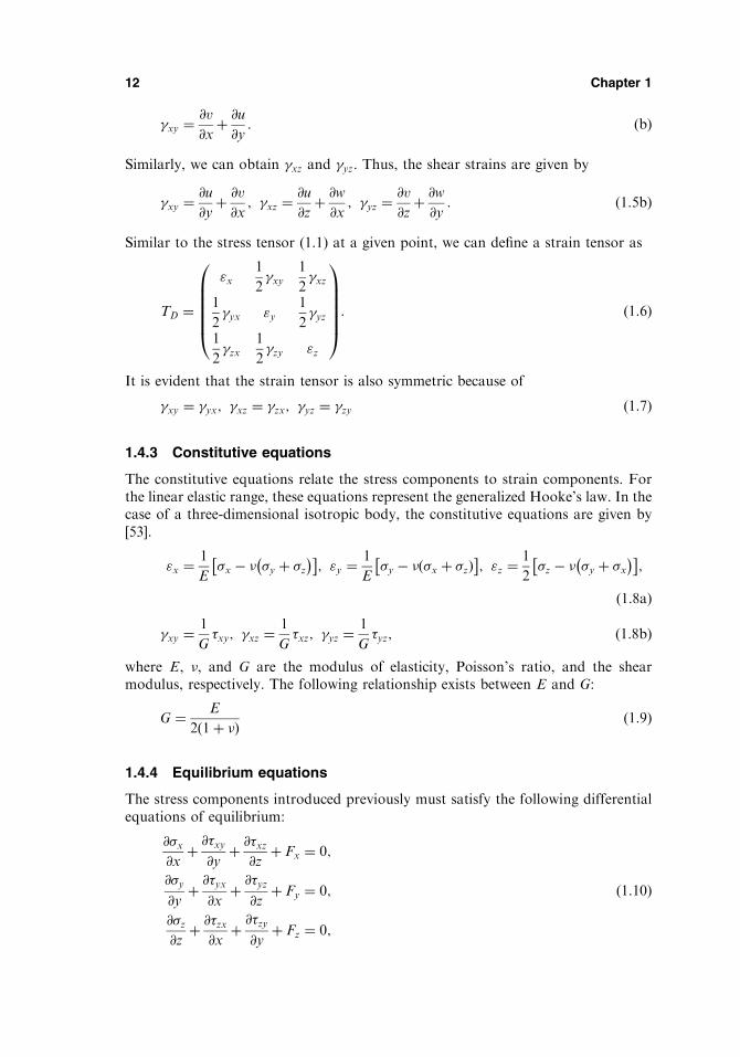
1.4.3 Constitutive equations

The constitutive equations relate the stress components to strain components. Forthe linear elastic range, these equations represent the generalized Hooke’s law. In thecase of a three-dimensional isotropic body, the constitutive equations are given by[53].

"x ¼ 1

E�x � � �y þ �z

� �� ; "y ¼

1

E�y � � �x þ �zð Þ� �

; "z ¼1

2�z � � �y þ �x

� �� ;

ð1:8aÞ

�xy ¼1

G�xy; �xz ¼

1

G�xz; �yz ¼

1

G�yz; ð1:8bÞ

where E, �, and G are the modulus of elasticity, Poisson’s ratio, and the shearmodulus, respectively. The following relationship exists between E and G:

G ¼ E

2ð1þ �Þ ð1:9Þ

1.4.4 Equilibrium equations

The stress components introduced previously must satisfy the following differentialequations of equilibrium:

@�x@x

þ @�xy@y

þ @�xz@z

þ Fx ¼ 0;

@�y@y

þ @�yx@x

þ @�yz@z

þ Fy ¼ 0;

@�z@z

þ @�zx@x

þ @�zy@y

þ Fz ¼ 0;

ð1:10Þ

12 Chapter 1

where Fx; Fy; and Fz are the body forces (e.g., gravitational, magnetic forces). Inderiving these equations, the reciprocity of the shear stresses, Eqs (1.7), has beenused.

1.4.5 Compatibility equations

Since the three equations (1.10) for six unknowns are not sufficient to obtain asolution, three-dimensional stress problems of elasticity are internally statically inde-terminate. Additional equations are obtained to express the continuity of a body.These additional equations are referred to as compatibility equations. In Eqs (1.5) wehave related the six strain components to the three displacement components.Eliminating the displacement components by successive differentiation, the follow-ing compatibility equations are obtained [53–55]:

@2"x@y2

þ @2"y

@x2¼ @2�xy@x@y

;

@2"y

@z2þ @

2"z@y2

¼ @2�yz@y@z

; ð1:11aÞ

@2"z@x2

þ @2"x@z2

¼ @2�xz@x@z

;

@

@z

@�yz@x

þ @�xz@y

� @�xy@z

� �¼ 2

@2"z@x@y

;

@

@x

@�xz@y

þ @�xy@z

� @�yz@x

� �¼ 2

@2"x@y@z

; ð1:11bÞ

@

@y

@�xy@z

þ @�yz@x

� @�xz@y

� �¼ 2

@2"y@x@z

:

For a two-dimensional state of stress (�z ¼ 0, �xz ¼ �yz ¼ 0), the equilibrium condi-tions (1.10) become

@�x@x

þ @�xy@y

þ Fx ¼ 0;

@�y@y

þ @�yx@x

þ Fy ¼ 0;

ð1:12Þ

and the compatibility equation is

@2"x@y2

þ @2"y

@x2¼ @2�xy@x@y

�xz ¼ �yz ¼ "z ¼ 0� �

: ð1:13Þ

We can rewrite Eq. (1.13) in terms of the stress components as follows

@2

@x2þ @2

@y2

!�x þ �y� � ¼ 0: ð1:14Þ

Introduction 13

17. Timoshenko, S.P., Sur la stabilite des systemes elastiques, Ann des Points et Chaussees,

vol. 13, pp. 496–566; vol. 16, pp. 73–132 (1913).

18. Timoshenko, S.P. and Woinowsky-Krieger, S., Theory of Plates and Shells, 2nd edn,

McGraw-Hill, New York, 1959.

19. Hencky, H., Der spanngszustand in rechteckigen platten (Diss.), Z Andew Math und

Mech, vol. 1 (1921).

20. Huber, M.T., Probleme der Static Techish Wichtiger Orthotroper Platten, Warsawa,

1929.

21. von Karman, T., Fesigkeitsprobleme in Maschinenbau, Encycl der Math Wiss, vol. 4, pp.

348–351 (1910).

22. von Karman,T., Ef Sechler and Donnel, L.H. The strength of thin plates in compression,

Trans ASME, vol. 54, pp. 53–57 (1932).

23. Nadai, A. Die formanderungen und die spannungen von rechteckigen elastischen platten,

Forsch a.d. Gebiete d Ingeineurwesens, Berlin, Nos. 170 and 171 (1915).

24. Foppl, A., Vorlesungen uber technische Mechanik, vols 1 and 2, 14th and 15th edns,

Verlag R., Oldenburg, Munich, 1944, 1951.

25. Gehring, F., Vorlesungen uber Mathematieche Physik, Mechanik, 2nd edn, Berlin,1877.

26. Boussinesq, J., Complements anne etude sur la theorie de l’equilibre et du mouvement

des solides elastiques, J de Math Pures et Appl , vol. 3, ses. t.5 (1879).

27. Leknitskii, S.G., Anisotropic Plates (English translation of the original Russian work),

Gordon and Breach, New York, 1968.

28. Reissner, E., The effect of transverse shear deformation on the bending of elastic plates, J

Appl Mech Trans ASME, vol. 12, pp. A69–A77 (1945).

29. Volmir, A.S., Flexible Plates and Shells, Gos. Izd-vo Techn.-Teoret. Lit-ry, Moscow,

1956 (in Russian).

30. Panov, D.Yu., On large deflections of circular plates, Prikl Matem Mech, vol. 5, No. 2,

pp. 45–56 (1941) (in Russian).

31. Bryan, G.N., On the stability of a plane plate under thrusts in its own plane, Proc London

Math Soc, 22, 54–67 (1981)

32. Cox, H.L, Buckling of Thin Plates in Compression, Rep. and Memor., No. 1553,1554,

(1933).

33. Hartmann, F., Knickung, Kippung, Beulung, Springer-Verlag, Berlin, 1933.

34. Dinnik, A.N., A stability of compressed circular plate, Izv Kiev Polyt In-ta, 1911 (in

Russian).

35. Nadai, A., Uber das ausbeulen von kreisfoormigen platten, Zeitschr VDJ, No. 9,10 (1915).

36. Meissner, E., Uber das knicken kreisfoormigen scheiben, Schweiz Bauzeitung, 101, pp. 87–

89 (1933).

37. Southwell, R.V. and Scan, S., On the stability under shearing forces of a flat elastic strip,

Proc Roy Soc, A105, 582 (1924).

38. Timoshenko, S.P. and Gere, J.M., Theory of Elastic Stability, 2nd edn, McGraw-Hill,

New York, 1961.

39. Karman, Th., Sechler, E.E. and Donnel, L.H., The strength of thin plates in compres-

sion, Trans ASME, 54, 53–57 (1952).

40. Levy, S., Bending of Rectangular Plates with Large Deflections, NACA, Rep. No.737,

1942.

41. Marguerre, K., Die mittragende briete des gedruckten plattenstreifens,

Luftfahrtforschung, 14, No. 3, 1937.

42. Gerard, G. and Becker, H., Handbook of Structural Stability, Part1 – Buckling of Flat

Plates, NACA TN 3781, 1957.

43. Volmir, A.S., Stability of Elastic Systems, Gos Izd-vo Fiz-Mat. Lit-ry, Moscow, 1963 (in

Russian).

44. Cox, H.l., The Buckling of Plates and Shells. Macmillan, New York, 1963.

Introduction 15

45. Voight, W, Bemerkungen zu dem problem der transversalem schwingungen rechteckiger

platten, Nachr. Ges (Gottingen), No. 6, pp. 225–230 (1893).

46. Ritz, W., Theorie der transversalschwingungen, einer quadratischen platte mit frein

randern, Ann Physic, Bd., 28, pp. 737–786 (1909).

47. Timoshenko, S.P. and Young, D.H., Vibration Problems in Engineering, John Wiley and

Sons., New York, 1963.

48. Den Hartog, J.P., Mechanical Vibrations, 4th edn, McGraw-Hill, New York, 1958.

49. Thompson, W.T., Theory of Vibrations and Applications, Prentice-Hill, Englewood Cliffs,

New Jersey, 1973.

50. Leissa, A.W., Vibration of Plates, National Aeronautics and Space Administration,

Washington, D.C., 1969.

51. Timoshenko, S.P., History of Strength of Materials, McGraw-Hill, New York, 1953.

52. Truesdell, C., Essays in the History of Mechanic., Springer-Verlag, Berlin, 1968.

53. Timoshenko, S.P. and Goodier, J.N., Theory of Elasticity, 3rd edn, McGraw-Hill, New

York, 1970.

54. Prescott, J.J., Applied Elasticity, Dover, New York, 1946.

55. Sokolnikoff, I.S., Mathematical Theory of Elasticity, 2nd edn, McGraw-Hill, New York,

1956.

16 Chapter 1

2

The Fundamentals of the Small-Deflection P late Bending Theory

2.1 INTRODUCTION

The foregoing assumptions introduced in Sec. 1.3 make it possible to derive the basicequations of the classical or Kirchhoff’s bending theory for stiff plates. It is conve-nient to solve plate bending problems in terms of displacements. In order to derivethe governing equation of the classical plate bending theory, we will invoke the threesets of equations of elasticity discussed in Sec. 1.4.

2.2 STRAIN–CURVATURE RELATIONS (KINEMATIC EQUATIONS)

We will use common notations for displacement, stress, and strain componentsadapted in elasticity (see Sec. 1.4). Let u; v; and w be components of the displacementvector of points in the middle surface of the plate occurring in the x; y, and zdirections, respectively. The normal component of the displacement vector, w (calledthe deflection), and the lateral distributed load p are positive in the downwarddirection. As it follows from the assumption (4) of Sec. 1.3

"z ¼ 0; �yz ¼ 0; �xz ¼ 0: ð2:1ÞIntegrating the expressions (1.5) for "z; �yz; and �xz and taking into account Eq.(2.1), we obtain

wz ¼ w x; yð Þ; uz ¼ �z@w

@xþ u x; yð Þ; vz ¼ �z

@w

@yþ v x; yð Þ; ð2:2Þ

where uz; vz, and wz are displacements of points at a distance z from the middlesurface. Based upon assumption (6) of Sec. 1.3, we conclude that u ¼ v ¼ 0. Thus,Eqs (2.2) have the following form in the context of Kirchhoff’s theory:

17

wz ¼ w x; yð Þ; uz ¼ �z@w

@x; vz ¼ �z

@w

@y: ð2:3Þ

As it follows from the above, the displacements uz and vz of an arbitrary horizontallayer vary linearly over a plate thickness while the deflection does not vary over thethickness.

Figure 2.1 shows a section of the plate by a plane parallel to Oxz; y ¼ const:,before and after deformation. Consider a segment AB in the positive z direction. Wefocus on an arbitrary point B which initially lies at a distance z from the undeformedmiddle plane (from the point A). During the deformation, point A displaces a dis-tance w parallel to the original z direction to point A1. Since the transverse sheardeformations are neglected, the deformed position of point B must lie on the normalto the deformed middle plane erected at point A1(assumption (4)). Its final position isdenoted by B1. Due to the assumptions (4) and (5), the distance z between the above-mentioned points during deformation remains unchanged and is also equal to z.

We can also represent the displacement components uz and vz, Eqs (2.2), in theform

uz ¼ �z#x; vz ¼ �z#y; ð2:4Þ

where

#x ¼ @w

@x; #y ¼

@w

@yð2:5Þ

are the angles of rotation of the normal (normal I–I in Fig. 2.1) to the middle surfacein the Oxz and Oyz plane, respectively. Owing to the assumption (4) of Sec. 1.3, #xand #y are also slopes of the tangents to the traces of the middle surface in the above-mentioned planes.

Substitution of Eqs (2.3) into the first two Eqs (1.5a) and into the first Eq.(1.5b), yields

"zx ¼ �z@2w

@x2; "zy ¼ �z

@2w

@y2; �zxy ¼ �2z

@2w

@x@y; ð2:6Þ

18 Chapter 2

Fig. 2.1

where the superscript z refers to the in-plane strain components at a point of theplate located at a distance z from the middle surface. Since the middle surfacedeformations are neglected due to the assumption (6), from here on, this superscriptwill be omitted for all the strain and stress components at points across the platethickness.

The second derivatives of the deflection on the right-hand side of Eqs. (2.6)have a certain geometrical meaning. Let a section MNP represent some plane curvein which the middle surface of the deflected plate is intersected by a plane y ¼ const.(Fig. 2.2).

Due to the assumption 3 (Sec. 1.3), this curve is shallow and the square of theslope angle may be regarded as negligible compared with unity, i.e., (@w=@xÞ2 � 1.Then, the second derivative of the deflection, @2w=@x2 will define approximately thecurvature of the section along the x axis, �x. Similarly, @2w=@y2 defines the curvatureof the middle surface �y along the y axis. The curvatures �x and �y characterize thephenomenon of bending of the middle surface in planes parallel to the Oxz and Oyzcoordinate planes, respectively. They are referred to as bending curvature and aredefined by

�x ¼1

�x¼ � @

2w

@x2; �y ¼

1

�y¼ � @

2w

@y2ð2:7aÞ

We consider a bending curvature positive if it is convex downward, i.e., in thepositive direction of the z axis. The negative sign is taken in Eqs. (2.7a) since, forexample, for the deflection convex downward curve MNP (Fig. 2.2), the secondderivative, @2w=@x2 is negative.

The curvature @2w=@x2 can be also defined as the rate of change of the angle#x ¼ @w=@x with respect to distance x along this curve. However, the above anglecan vary in the y direction also. It is seen from comparison of the curves MNP andM1N1P1 (Fig. 2.2), separated by a distance dy. If the slope for the curve MNPis @w=@x then for the curve M1N1P1 this angle becomes equal to@w

@x� @

@y

@w

@x

� �dy

� �or

@w

@x� @2w

@x@ydy

!. The rate of change of the angle @w=@x per

unit length will be ð�@2w=@x@y). The negative sign is taken here because it is assumed

Small-Deflection Plate Bending Theory 19

Fig. 2.2

tions of equilibrium for a plate element under a general state of stress (1.10) (assum-ing that the body forces are zero) serve well for this purpose, however. If the faces ofthe plate are free of any tangent external loads, then �xz and �yz are zero forz ¼ �h=2. From the first two Eqs (1.10) and Eqs (2.9) and (2.10), the shear stresses�xz (Fig. 2.3(b)) and �yz are

�xz ¼ �ðh=2

�h=2

@�x@x

þ @�xy@y

� �dz ¼ E z2 � h2=4

� �2 1� �2� � @

@xr2w;

�yz ¼ �ðh=2

�h=2

@�y@y

þ @�yx@x

� �dz ¼ E z2 � h2=4

� �2 1� �2� � @

@yr2w;

ð2:16Þ

where r2ð Þ is the Laplace operator, given by

r2w ¼ @2w

@x2þ @

2w

@y2: ð2:17Þ

It is observed from Eqs (2.15) and (2.16) that the stress components �x; �y;and �xy (in-plane stresses) vary linearly over the plate thickness, whereas the shearstresses �xz and �yz vary according to a parabolic law, as shown in Fig. 2.5.

The component �z is determined by using the third of Eqs (1.10), upon sub-stitution of �xz and �yz from Eqs (2.16) and integration. As a result, we obtain

�z ¼ � E

2ð1� �2Þh3

12� h2z

4þ z3

3

!r2r2w: ð2:18Þ


Fig. 2.5

2.4 GOVERNING EQUATION FOR DEFLECTION OF PLATES INCARTESIAN COORDINATES

The components of stress (and, thus, the stress resultants and stress couples) gen-erally vary from point to point in a loaded plate. These variations are governed bythe static conditions of equilibrium.

Consider equilibrium of an element dx dy of the plate subject to a verticaldistributed load of intensity pðx; yÞ applied to an upper surface of the plate, as shownin Fig. 2.4. Since the stress resultants and stress couples are assumed to be applied tothe middle plane of this element, a distributed load p x; yð Þ is transferred to themidplane. Note that as the element is very small, the force and moment componentsmay be considered to be distributed uniformly over the midplane of the plate ele-ment: in Fig. 2.4 they are shown, for the sake of simplicity, by a single vector. Asshown in Fig. 2.4, in passing from the section x to the section xþ dx an intensity ofstress resultants changes by a value of partial differential, for example, by@Mx ¼ @Mx

@x dx. The same is true for the sections y and yþ dy. For the system offorces and moments shown in Fig. 2.4 , the following three independent conditionsof equilibrium may be set up:

(a) The force summation in the z axis gives

@Qx

@xdxdyþ @Qy

@ydxdyþ pdxdy ¼ 0;

from which

@Qx

@xþ @Qy

@yþ p ¼ 0: ð2:19Þ

(b) The moment summation about the x axis leads to

@Mxy

@xdxdyþ @My

@ydxdy�Qydxdy ¼ 0

or

@Mxy

@xþ @My

@y�Qy ¼ 0: ð2:20Þ

Note that products of infinitesimal terms, such as the moment of the loadp and the moment due to the change in Qy have been omitted in Eq.(2.20) as terms with a higher order of smallness.

(c) The moment summation about the y axis results in

@Myx

@yþ @Mx

@x�Qx ¼ 0: ð2:21Þ

It follows from the expressions (2.20) and (2.21), that the shear forces Qx and Qy canbe expressed in terms of the moments, as follows:

Qx ¼ @Mx

@xþ @Mxy

@yð2:22aÞ

24 Chapter 2

Qy ¼@Mxy

@xþ @My

@yð2:22bÞ

Here it has been taken into account thatMxy ¼ Myx: Substituting Eqs (2.22) into Eq.(2.19), one finds the following:

@2Mx

@x2þ 2

@2Mxy

@x@yþ @

2My

@y2¼ �pðx; yÞ: ð2:23Þ

Finally, introduction of the expressions for Mx; My; and Mxy from Eqs (2.13) intoEq. (2.23) yields

@4w

@x4þ 2

@4w

@x2@y2þ @

4w

@y4¼ p

D: ð2:24Þ

This is the governing differential equation for the deflections for thin plate bendinganalysis based on Kirchhoff’s assumptions. This equation was obtained by Lagrangein 1811. Mathematically, the differential equation (2.24) can be classified as a linearpartial differential equation of the fourth order having constant coefficients [1,2].

Equation (2.24) may be rewritten, as follows:

r2ðr2wÞ ¼ r4w ¼ p

D; ð2:25Þ

where

r4ð Þ � @4

@x4þ 2

@4

@x2@y2þ @4

@y4ð2:26Þ

is commonly called the biharmonic operator.Once a deflection function wðx; yÞ has been determined from Eq. (2.24), the

stress resultants and the stresses can be evaluated by using Eqs (2.13) and (2.15). Inorder to determine the deflection function, it is required to integrate Eq. (2.24) withthe constants of integration dependent upon the appropriate boundary conditions.We will discuss this procedure later.

Expressions for the vertical forces Qx and Qy, may now be written in terms ofthe deflection w from Eqs (2.22) together with Eqs (2.13), as follows:

Qx ¼ �D@

@x

@2w

@x2þ @

2w

@y2

!¼ �D

@

@xðr2wÞ;

Qy ¼ �D@

@y

@2w

@x2þ @

2w

@y2

!¼ �D

@

@yðr2wÞ:

ð2:27Þ

Using Eqs (2.27) and (2.25), we can rewrite the expressions for the stress components�xz; �yz; and �z, Eqs (2.16) and (2.18), as follows

�xz ¼3Qx

2h1� 2z

h

� �2" #

; �yz ¼3Qy

2h1� 2z

h

� �2" #

;


�z ¼ � 3p

4

2

3� 2z

hþ 1

3

2z

h

� �3" #

: ð2:28Þ

The maximum shear stress, as in the case of a beam of rectangular cross section,occurs at z ¼ 0 (see Fig. 2.5), and is represented by the formula

max :�xz ¼3

2

Qx

h; max :�yz ¼

3

2

Qy

h:

It is significant that the sum of the bending moments defined by Eqs (2.13) isinvariant; i.e.,

Mx þMy ¼ �Dð1þ �Þ @2w

@x2þ @

2w

@y2

!¼ �Dð1þ �Þr2w

or

Mx þMy

1þ � ¼ �Dr2w ð2:29Þ

Letting M denote the moment function or the so-called moment sum,

M ¼ Mx þMy

1þ � ¼ �Dr2w; ð2:30Þ

the expressions for the shear forces can be written as

Qx ¼ @M

@x; Qy ¼

@M

@yð2:31Þ

and we can represent Eq. (2.24) in the form

@2M

@x2þ @

2M

@y2¼ �p;

@2w

@x2þ @

2w

@y2¼ �M

D:

ð2:32Þ

Thus, the plate bending equation r4w ¼ p=D is reduced to two second-order partialdifferential equations which are sometimes preferred, depending upon the method ofsolution to be employed.

Summarizing the arguments set forth in this section, we come to the conclusionthat the deformation of a plate under the action of the transverse load pðx; yÞ appliedto its upper plane is determined by the differential equation (2.24). This deformationresults from:

(a) bending produced by bending moments Mx and My, as well as by theshear forces Qx and Qy;

(b) torsion produced by the twisting moments Mxy ¼ Myz.

Both of these phenomena are generally inseparable in a plate. Indeed, let us replacethe plate by a flooring composed of separate rods, each of which will bend under the

26 Chapter 2

action of the load acting on it irrespective of the neighboring rods. Let them now betied together in a solid slab (plate). If we load only one rod, then, deflecting, it willcarry along the adjacent rods, applying to their faces those shear forces which wehave designated here by Qx and Qy. These forces will cause rotation of the crosssection, i.e., twisting of the rod. This approximation of a plate with a grillage of rods(or beams) is known as the ‘‘grillage, or gridwork analogy’’ [3].

2.5 BOUNDARY CONDITIONS

As pointed out earlier, the boundary conditions are the known conditions on thesurfaces of the plate which must be prescribed in advance in order to obtain thesolution of Eq. (2.24) corresponding to a particular problem. Such conditionsinclude the load pðx; yÞ on the upper and lower faces of the plate; however, theload has been taken into account in the formulation of the general problem ofbending of plates and it enters in the right-hand side of Eq. (2.24). It remains toclarify the conditions on the cylindrical surface, i.e., at the edges of the plate,depending on the fastening or supporting conditions. For a plate, the solution ofEq. (2.24) requires that two boundary conditions be satisfied at each edge. Thesemay be a given deflection and slope, or force and moment, or some combination ofthese.

For the sake of simplicity, let us begin with the case of rectangular plate whoseedges are parallel to the axes Ox and Oy. Figure 2.6 shows the rectangular plate oneedge of which (y ¼ 0) is built-in, the edge x ¼ a is simply supported, the edge x ¼ 0 issupported by a beam, and the edge y ¼ b is free.

We consider below all the above-mentioned boundary conditions:(1) Clamped, or built-in, or fixed edge y ¼ 0At the clamped edge y ¼ 0 the deflection and slope are zero, i.e.,

w ¼ 0jy¼0 and #y �@w

@y¼ 0

y¼0

: ð2:33Þ

(2) Simply supported edge x ¼ aAt these edges the deflection and bending moment Mx are both zero, i.e.,

w ¼ 0jx¼a; Mx ¼ �D@2w

@x2þ � @

2w

@y2

!¼ 0

x¼a

: ð2:34Þ

The first of these equations implies that along the edge x ¼ a all the derivativesof w with respect to y are zero, i.e., if x ¼ a and w ¼ 0, then @w

@y ¼ @2w@y2

¼ 0.It follows that conditions expressed by Eqs (2.34) may appear in the following

equivalent form:

w ¼ 0jx¼a;@2w

@x2¼ 0

x¼a

: ð2:35Þ

(3) Free edge y ¼ bSuppose that the edge y ¼ b is perfectly free. Since no stresses act over this

edge, then it is reasonable to equate all the stress resultants and stress couplesoccurring at points of this edge to zero, i.e.,


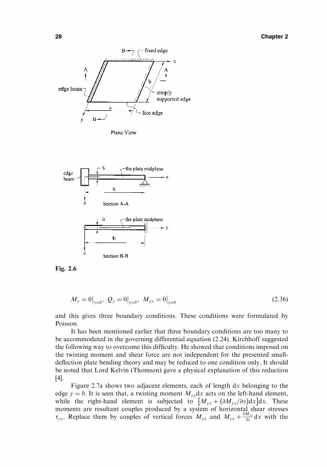
My ¼ 0y¼b; Qy ¼ 0

y¼b; Myx ¼ 0

y¼b

ð2:36Þ

and this gives three boundary conditions. These conditions were formulated byPoisson.

It has been mentioned earlier that three boundary conditions are too many tobe accommodated in the governing differential equation (2.24). Kirchhoff suggestedthe following way to overcome this difficulty. He showed that conditions imposed onthe twisting moment and shear force are not independent for the presented small-deflection plate bending theory and may be reduced to one condition only. It shouldbe noted that Lord Kelvin (Thomson) gave a physical explanation of this reduction[4].

Figure 2.7a shows two adjacent elements, each of length dx belonging to theedge y ¼ b. It is seen that, a twisting moment Myxdx acts on the left-hand element,while the right-hand element is subjected to Myx þ @Myx=@x

� �dx

� �dx. These

moments are resultant couples produced by a system of horizontal shear stresses�yx. Replace them by couples of vertical forces Myx and Myx þ @Myx

@x dx with the

28 Chapter 2

Fig. 2.6

moment arm dx having the same moment (Fig. 2.7b), i.e., as if rotating the above-mentioned couples of horizontal forces through 90.

Such statically equivalent replacement of couples of horizontal forces by cou-ples of vertical forces is well tolerable in the context of Kirchhoff’s plate bendingtheory. Indeed, small elements to which they are applied can be considered as abso-lutely rigid bodies (owing to assumption (4)). It is known that the above-mentionedreplacement is quite legal for such a body because it does not disturb the equilibriumconditions, and any moment may be considered as a free vector.

Forces Myx and Myx þ @Myx

@x dx act along the line mn (Fig. 2.7b) in oppositedirections. Having done this for all elements of the edge y ¼ b we see that at theboundaries of two neighboring elements a single unbalanced force ð@Myx=@xÞdx isapplied at points of the middle plane (Fig. 2.7c).

Thus, we have established that the twisting momentMyx is statically equivalentto a distributed shear force of an intensity @Myx=@x along the edge y ¼ b, for asmooth boundary. Proceeding from this, Kirchhoff proposed that the three bound-ary conditions at the free edge be combined into two by equating to zero the bendingmoment My and the so-called effective shear force per unit length Vy. The latter isequal to the sum of the shear force Qy plus an unbalanced force @Myx=@x, whichreflects the influence of the twisting moment Myx (for the edge y ¼ b). Now we arriveat the following two conditions at the free edge:

My ¼ 0y¼b; Vy ¼ 0

y¼b

ð2:37Þ

where

Vy ¼ Qy þ@Mxy

@x: ð2:38Þ

The effective shear force Vy can be expressed in terms of the deflection w using Eqs(2.13) and (2.27). As a result, we obtain


Fig. 2.7

Vy ¼ �D@

@y

@2w

@y2þ ð2� �Þ @

2w

@x2

" #: ð2:39aÞ

In a similar manner, we can obtain the effective shear force at the edge parallelto the x axis, i.e.,

Vx ¼ �D@

@x

@2w

@x2þ ð2� �Þ @

2w

@y2

" #ð2:39bÞ

Finally, the boundary conditions (2.37) may be rewritten in terms of the deflec-tion as follows

@2w

@y2þ � @

2w

@x2¼ 0

y¼b

and� @

@y

@2w

@y2þ ð2� �Þ @

2w

@x2

" #¼ 0

y¼b

: ð2:40Þ

Similarly, the boundary conditions for the free edge parallel to the x axis can beformulated. This form of the boundary conditions for a free edge is conventional.

It should be noted that transforming the twisting moments – as it was men-tioned above – we obtain not only continuously distributed edge forces Vx and Vy

but, in addition, also nonvanishing, finite concentrated forces at corner points (oneach side of a corner) of a rectangular plate. These are numerically equal to the valueof the corresponding twisting moment (Fig. 2.8). The direction and the total magni-tude of the corner forces can be established by analyzing boundary conditions of aplate and the deflection surface produced by a given loading.

The concept of the corner forces is not limited to the intersection of two freeboundaries, where they obviously must vanish. In general, any right angle cornerwhere at least one of the intersecting boundaries can develop Mxy and Myx will havea corner force. Consider, as an example, the case of symmetrically loaded, simplysupported rectangular plate, as shown in Fig. 2.9.

At the corners, x ¼ a and y ¼ b, the above-discussed action of the twistingmoments (because Mxy ¼ Myx) results in

30 Chapter 2

Fig. 2.8

S ¼ 2Mxy ¼ �2D 1� �ð Þ @2w

@x@y

x¼a;y¼b

: ð2:41Þ

Thus, the distributed twisting moments are statically equivalent to the distributededge forces @Myx=@x and @Mxy=@y over the plate boundary, as well as to the con-centrated corner forces, S ¼ 2Mxy for a given rectangular plate. Note that the direc-tions of the concentrated corner forces, S, are shown in Fig. 2.9 for a symmetricaldownward directed loading of the plate. At the origin of the coordinate system,taking into account the nature of torsion of an adjacent element, we obtain forthe moment Mxy and, consequently, for the force S, the minus sign. If we rotatethe twisting moment Mxy < 0 through 90, then we obtain at this corner point(x ¼ 0; y ¼ 0) a downward force S ¼ 2Mxy. At other corner points the signs ofMxy will alternate, but the above-mentioned corner forces will be directed downwardeverywhere for a symmetrical loading of a plate.

The concentrated corner force for plates having various boundary conditionsmay be determined similarly. In general, any right angle corner where at least one ofthe intersecting boundaries can develop Mxy or Myx will have a corner force. Forinstance, when two adjacent plate edges are fixed or free, we have S ¼ 0, since alongthese edges no twisting moments exist. If one edge of a plate is fixed and another one(perpendicular to the fixed edge) is simply supported, then S ¼ Mxy. The case ofnon-right angle intersections will be examined later.

It is quite valid to utilize the above replacement of the shear force Qy andtwisting moment Mxy by the effective shear force Vy in the context of theapproximate Kirchhoff’s theory of plate bending, as it was mentioned earlier.But with respect to a real plate, equating of the effective shear force to zerodoes not mean that both the shear force and twisting moment are necessarilyequal to zero. Hence, according to Kirchhoff’s theory, we obtain such a solutionwhen along a free edge, e.g., y ¼ const, some system of shear stresses �yz (corre-sponding to Qy) and �yx (corresponding to Myx) is applied (of course, such asystem of stresses and corresponding to them the stress resultants and stresscouples appear on this free edge). This system is mutually balanced on theedge y ¼ const and it causes an additional stress field. The latter, however, due


Fig. 2.9

dQb

dyð0; yÞ ¼ � EIð Þb

@4wb

@y4ð0; yÞ and ðbÞ

Tð0; yÞ ¼ � GJð Þbd#bdy

ð0; yÞ ¼ � GJð Þb@2wb

@x@yð0; yÞ; ðcÞ

where ðEIÞb and ðGJÞb are the flexural rigidity and the torsional stiffness of the beamcross section, respectively.

Substituting (b) and (c) into Eq. (a) and taking into account the compatibilityconditions (2.42), gives the boundary conditions for the plate edge x ¼ 0 supportedby the beam:

Vx ¼ � EIð Þb@4wb

@y4

x¼0

; Mx ¼ � GJð Þb@3wb

@x@y2

x¼0

ð2:43aÞ

Using the expressions for Mx and Vx, Eqs. (2.13), (2.39b), and Eqs (2.42), we canrewrite the boundary conditions (2.43a) in terms of w, as follows:

D@3w

@x3þ ð2� �Þ @

3w

@x@y2

" #¼ EIð Þb

@4w

@y4

x¼0

; D@2w

@x2þ � @

2w

@y2

" #¼ GJð Þb

@3w

@x@y2

x¼0

:

ð2:43bÞSimilar expressions can be written for edges y ¼ 0; b.

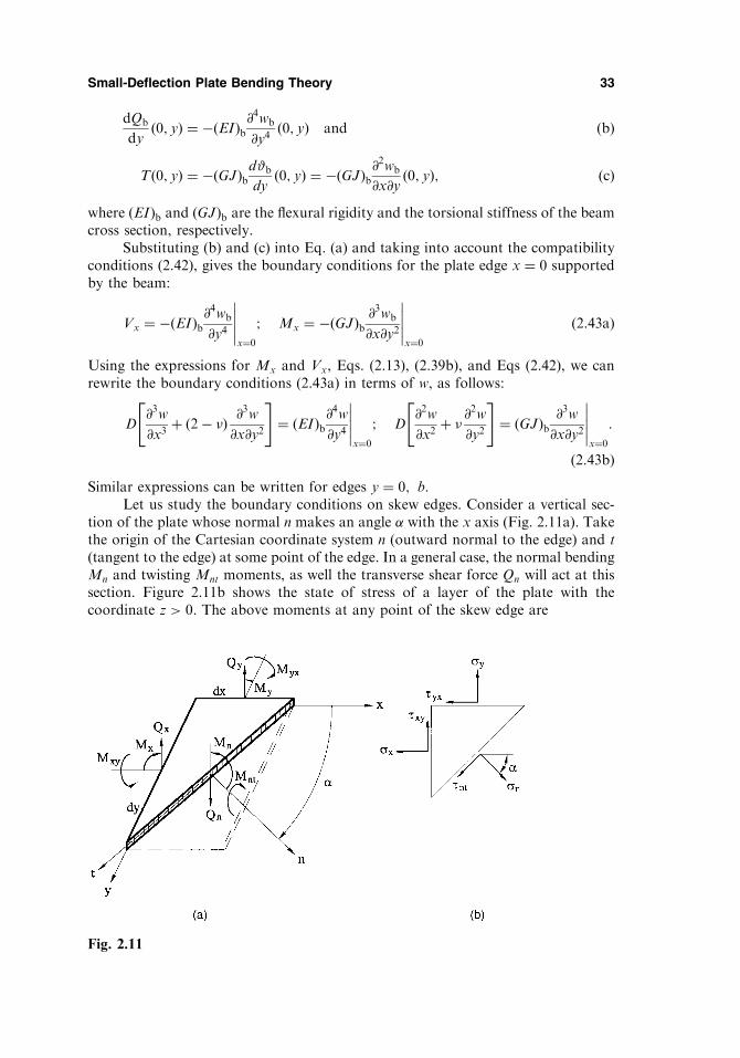
Let us study the boundary conditions on skew edges. Consider a vertical sec-tion of the plate whose normal n makes an angle with the x axis (Fig. 2.11a). Takethe origin of the Cartesian coordinate system n (outward normal to the edge) and t(tangent to the edge) at some point of the edge. In a general case, the normal bendingMn and twisting Mnt moments, as well the transverse shear force Qn will act at thissection. Figure 2.11b shows the state of stress of a layer of the plate with thecoordinate z > 0. The above moments at any point of the skew edge are


Fig. 2.11

2.6 VARIATIONAL FORMULATION OF PLATE BENDING PROBLEMS

It is known from the theory of elasticity that governing equations for stresses,strains, and displacements can be represented in the differential form. However,this is not a unique possible formulation of the problem for finding the stress–strainfield of an elastic body. The problem of determining stresses, strains, and displace-ments can be reduced to some definite integral of one or another type of thesefunctions called functionals. Then, the functions themselves (stresses, strains, anddisplacements) reflecting a real state of a body can be found from conditions ofextremum for this functional. The mathematical techniques of such an approach isstudied in the division of mathematics called the calculus of variation. Therefore,some postulates and statements that formulate properties of these functionals in thetheory of elasticity are referred to as variational principles. The latter represent somebasic theorems expressed in the form of integral equalities connecting stresses,strains, and displacements throughout the volume of a body and based on theproperties of the work done by external and internal forces. A variety of powerfuland efficient approximate methods for analysis of various linear and nonlinear pro-blems of solid mechanics are based on the variational principles. Some of thesemethods will be described further in Chapter 6.

2.6.1 Strain energy of plates

A functional is a scalar quantity depending on some function or several functions, asfrom independent variables. The functional can be treated as a function of an infinitenumber of independent variables. The subject matter of the calculus of variation issearching of unknown functions fiðx; y; zÞ that give a maximum (minimum) or sta-tionary value of a functional. For example,

� ¼ð ðV

ðF f1ðx; y; zÞ; f2ðx; y; zÞ; . . . ; fnðx; y; zÞ; f 0

1 ðx; y; zÞ; . . . ;�

f 0n ðx; y; zÞ; x; y; z

�dV:

The above-mentioned functions for which the functional is maximum (minimum) orstationary are referred to as extremals of the given functional [8–11].

Let us consider a functional expressing the total potential energy of a deformedelastic body and the loads acting on it. The total potential energy, �, consists of thestrain energy of deformation (the potential of internal forces), U, and the potentialenergy of external forces (the potential of external forces), �, i.e.,

� ¼ U þ�: ð2:50Þ

By convention, let us assume that the potential energy at the initial, undeformedstate, �0, is zero. Hence, the total energy � presents a variation of the energy ofinternal and external forces in the transition from initial to deformed states. Thepotential energy of a body is measured by the work done by external and internalforces when this body returns from its final to an initial position (where it wasmentioned above, �0 ¼ 0).

Our study is mainly limited to linearly elastic bodies that dissipate no energyand have only one equilibrium configuration. We also require that loads keep the

36 Chapter 2

� ¼ 1

2

ð ðA

D@2w

@x2þ @

2w

@y2

!2

� 2ð1� �Þ @2w

@x2@2w

@y2� @2w

@x@y

!224

35

8<:

9=;dA

�ð ðA

pðx; yÞwdAþXi

Pwi þXj

Mj#jþ24

þ�

Vnwn þmn

@w

@nþmnt

@w

@t

� �ds

35;

ð2:60Þ

or alternatively

� ¼ 1

2

ð ðA

Mx�x þMy�y þ 2Mxy�xy� �

dA

�ð ðA

pðx; yÞwdAþXi

Piwi þXj

Mj#jþ24

þ�

Vnwn þmn

@w

@nþmnt

@w

@t

� �ds

35:

ð2:61Þ

As is seen from Eq. (2.58) that the value of the total potential energy ofbending of plates is determined by an assignment of deflection w as a function ofindependent variables (x and y in the Cartesian coordinate system).

2.6.2 Variational principles

Let us consider some general concepts of the calculus of variation. A variation meansan infinitesimal increment of a function for fixed values of its independent variables.The variation is designated by the symbol �. The variational symbol � may be treatedas the differential operator d. The only difference between them lies in the fact thatthe symbol � refers to some possible variations of a given function while the symbol dis associated with real variations of the same function. In what follows, only thefollowing three operations are needed:

dð�wÞdx

¼ �dw

dx

� �; �ðw2Þ ¼ 2wð�wÞ;

ðð�wÞdx ¼ �

ðwdx:

Consider an elastic body in equilibrium. This means that the body subjectedto the maximum values of static (i.e., slowly piled-up) external forces has alreadyreached its final state of deformation. Now we disturb this equilibrium conditionby introducing small, arbitrary, but kinematically compatible, displacements.These displacements need not actually take place and need not be infinitesimal.Only one restriction is imposed on these displacements: they must be compatiblewith the support conditions (as discussed later, there are cases when satisfactionof geometric (or kinematic) boundary conditions is sufficient) and internal com-patibility of the body. These displacements are called admissible virtual, because


brium. Hence, in this case, the total potential energy of a given system has a mini-mum. From the uniqueness theorem [6,7], the problem of the theory of elasticity,based on assumptions of small displacements and deformations defines only oneequilibrium configuration, and this configuration of equilibrium is stable. Thus, ifthe small-deflection theory of an elastic body is being studied, then the potentialenergy is a minimum in an equilibrium state. So, the principle of minimum potentialenergy, proposed by Lagrange, can be formulated, as follows:

Among all admissible configurations of an elastic body, the actual configuration (that

satisfies static equilibrium conditions) makes the total potential energy, �, stationary

with respect to all small admissible virtual displacements. For stable equilibrium, � is a

minimum.

Notice that the above principle applies to a conservative system only.It can be shown that the governing differential equation (2.24) and the bound-

ary conditions (2.48) can be deduced from Lagrange’s variational principle (2.64)[3,8–12]. However, the key importance of the variational principles discussed aboveis that they can be used to obtain approximate solutions of complicated problems ofsolid mechanics, in particular, plate-shell bending problems. These are obtainedwhile avoiding mathematical difficulties associated with integration of differentialequations in partial derivatives. The corresponding methods, called variational meth-ods and based on the above-mentioned principles, are discussed further in Chapter 6.More complete information on the variational principles and their application inmechanics is available in the literature [8–12].

PROBLEMS

2.1 Verify the result given by Eq. (2.18).

2.2 Derive the governing differential equation for deflections of a plate subjected to a

distributed moment load mxðx; yÞ and myðx; yÞ applied to the middle surface.

2.3 Show that at the corner of a polygonal simply supported plate, Mxy ¼ 0 unless the

corner is 90.2.4 If a lateral deflection w is a known function of x and y, what are the maximum slope

@w=@n and the direction of axis n with respect to the x axis in terms of @w=@x and

@w=@y?2.5 Show that the sum of bending curvatures in any two mutually perpendicular directions,

n and t, at any point of the middle surface, is a constant, i.e.,

�x þ �y ¼ �n þ �t ¼ const:

2.6 Verify the expression given by Eq. (2.61).

2.7 Derive the expressions for the boundary quantities Mn;Mnt; and Vn in terms of the

deflection w at a regular (smooth) point of the curvilinear contour of the plate using:

(a) the local coordinates n and t where the coordinate n coincides with the direction of

the outward normal and t – with the tangent direction to the boundary; (b) the intrinsic

coordinates n and s, where s, is the arc length over the boundary.

Hint: use the following relations for part (b)

@n

@s¼ 1

�t;@t

@s¼ � 1

�n

where n and t are the unit vectors of the intrinsic coordinate system directed along the

outward normal and tangent to the boundary, respectively.


2.8 Derive Eq. (2.24) directly from the third equation of (1.10) by using the relations (2.16)

and (2.17).

2.9 Assume that shear stresses in the plate are distributed according to the parabolic law

for �h=2 � z � h=2. Show that when the expression �xz ¼ 6Qx=h3

� �h=2ð Þ2�z2

� �is sub-

stituted into the first relation (2.12) an identity is obtained.

2.10 Prove that the integral (2.56) is equal to zero for fixed supports and for simply sup-

ported edges.

REFERENCES

1. Webster, A.G., Partial Differential Equations of Mathematical Physics, Dover, New

York, 1955.

2. Sommerfeld, A., Partial Differential Equations in Physics, Academic Press, New York,

1948.



4. Thomson, W. and Tait, P.G., Treatise on Natural Philosophy, Cambridge University

Press, Cambridge, 1890.

5. Timoshenko, S.P., Strength of Materials, 3rd edn, Van Nostrand Company, New York,

1956.

6. Timoshenko, S.P. and Goodier, J.N., Theory of Elasticity, 3rd edn, McGraw-Hill, New

York, 1970.

7. Prescott, J.J., Applied Elasticity, Dover, New York, 1946.

8. Forray, M.J., Variational Calculus in Science and Engineering, McGraw-Hill, New York,

1968.

9. Lanczos, C., The Variational Principles of Mechanics, The University of Toronto Press,

Toronto, 1964.

10. Hoff, H.I., The Analysis of Structures Based on the Minimal Principles and Principle of

Virtual Displacements, John Wiley and Sons, New York, 1956.

11. Reddy, J.N., Energy and Variational Methods in Applied Mechanics, John Wiley and

Sons, New York, 1984.

12. Washizy, K., Variational Methods in Elasticity and Plasticity, 3rd edn, Pergamon Press,

New York, 1982.

FURTHER READING

Gould, P.L., Analysis of Shells and Plates, Springer-Verlag, New York, Berlin, 1988.

Heins, C.P., Applied Plate Theory for the Engineer, Lexington Books, Lexington,

Massachusetts, 1976.

McFarland, D.E., Smith, B.L. and Bernhart, W.D., Analysis of Plates, Spartan Books, New

York, 1972.

Mansfield, E.H., The Bending and Stretching of Plates, Macmillan, New York, 1964.

Szilard, R., Theory and Analysis of Plates, Prentice-Hall, Inc., Englewood Cliffs, New York,

1974.

Ugural, A.C., Stresses in Plates and Shells, McGraw-Hill, New York, 1981.

Vinson, J.R., The Behavior of Plates and Shells, John Wiley and Sons, New York, 1974.

42 Chapter 2

3

Rectangular Plates

3.1 INTRODUCTION

We begin the application of the developed plate bending theory with thin rectangularplates. These plates represent an excellent model for development and as a check ofvarious methods for solving the governing differential equation (2.24).

In this chapter we consider some mathematically ‘‘exact’’ solutions in the formof double and single trigonometric series applied to rectangular plates with varioustypes of supports and transverse loads, plates on an elastic foundation, continuousplates, etc.

3.2 THE ELEMENTARY CASES OF PLATE BENDING

Let us consider some elementary examples of plate bending of great importance forunderstanding how a plate resists the applied loads in bending. In addition, theseelementary examples enable one to obtain closed-form solutions of the governingdifferential equation (2.24).

3.2.1 Cylindrical bending of a plate

Consider an infinitely long plate in the y axis direction. Assume that the plate issubjected to a transverse load which is a function of the variable x only, i.e., p ¼ pðxÞ(Fig. 3.1a). In this case all the strips of a unit width parallel to the x axis and isolatedfrom the plate will bend identically. The plate as a whole is found to be bent over thecylindrical surface w ¼ wðxÞ. Setting all the derivatives with respect to y equal zero inEq. (2.24), we obtain the following equation for the deflection:

d4w

dx4¼ pðxÞ

D: ð3:1Þ

43

Using Eqs (2.13), (3.8), and (3.9), we obtain

C1 ¼�m2 �m1

Dð1� �2Þ ; C2 ¼�m1 �m2

Dð1� �2Þ :

Substituting the above into Eq. (3.8) yields the deflection surface, as shown below:

w ¼ 1

2Dð1� �2Þ ð�m2 �m1Þx2 þ ð�m1 �m2Þy2� � ð3:10Þ

Hence, in all sections of the plate parallel to the x and y axes, only the constantbending moments Mx ¼ m1 and My ¼ m2 will act. Other stress resultants and stresscouples are zero, i.e.,

Mxy ¼ Qx ¼ Qy ¼ 0:

This case of bending of plates may be referred to as a pure bending.Let us consider some particular cases of pure bending of plates.

(a) Let m1 ¼ m2 ¼ m.Then,

w ¼ � m

2Dð1þ �Þ ðx2 þ y2Þ: ð3:11Þ

This is an equation of the elliptic paraboloid of revolution. The curved plate in thiscase represents a part of a sphere because the radii of curvature are the same at allthe planes and all the points of the plate.

(b) Let m1 ¼ m;m2 ¼ 0 (Fig. 3.3).Then,

w ¼ m

2Dð1� �2Þ �x2 þ �y2� �: ð3:12Þ

A surface described by this equation has a saddle shape and is called the hyperbolicparaboloid of revolution (Fig. 3.3). Horizontals of this surface are hyperbolas, asymp-totes of which are given by the straight lines x

y¼ � ffiffiffi

�p

. As is seen, due to the Poissoneffect the plate bends not only in the plane of the applied bending moment Mx ¼m1 ¼ m but it also has an opposite bending in the perpendicular plane.

46 Chapter 3

Fig. 3.3

(c) Let m1 ¼ m;m2 ¼ �m (Fig. 3.4a).Then

w ¼ m

2Dð1� �Þ ð�x2 þ y2Þ: ð3:13Þ

This is an equation of an hyperbolic paraboloid with asymptotes inclined at 45 to thex and y axes.

Let us determine the moments Mn and Mnt from Eqs (2.45) in skew sectionsthat are parallel to the asymptotes. Letting ¼ 45, we obtain

Mn ¼ 0; Mnt ¼ �m:

Thus, a part of the plate isolated from the whole plate and equally inclined to the xand y axes will be loaded along its boundary by uniform twisting moments ofintensity m. Hence, this part of the plate is subjected to pure twisting (Fig. 3.4b).Let us replace the twisting moments by the effective shear forces V, rotating thesemoments through 90 (see Sec. 2.4). Along the whole sides of the isolated part weobtain V ¼ 0, but at the corner points the concentrated forces S ¼ 2m are applied.Thus, for the model of Kirchhoff’s plate, an application of self-balanced concen-trated forces at corners of a rectangular plate produces a deformation of pure torsionbecause over the whole surface of the plate Mnt ¼ m ¼ const:

Remark

Since the plate described above in pure bending has no supports, its deflectionshave been determined with an accuracy of the displacements of an absolutely rigidbody.

3.3 NAVIER’S METHOD (DOUBLE SERIES SOLUTION)

In 1820, Navier presented a paper to the French Academy of Sciences on the solu-tion of bending of simply supported plates by double trigonometric series [1].

Rectangular Plates 47

Fig. 3.4

It can be shown by direct integration that

ða0

sinm�x

asin

l�x

adx ¼

0 ifm 6¼ l

a=2 if m ¼ l

8<:

and

ðb0

sinn�y

bsin

k�y

bdy ¼

0 if n 6¼ k

b=2 if n ¼ k:

8<:

ð3:16Þ

The coefficients of the double Fourier expansion are therefore the following:

pmn ¼4

ab

ða0

ðb0

pðx; yÞ sinm�xa

sinn�y

bdxdy: ð3:17Þ

Since the representation of the deflection (3.15a) satisfies the boundary conditions(3.14), then the coefficients wmn must satisfy Eq. (2.24). Substitution of Eqs (3.15)into Eq. (2.24) results in the following equation:

X1m¼1

X1n¼1

wmn

m�

a

� �4þ 2

m�

a

� �2 n�

b

� �2þ n�

b

� �4� �� pmn

D

�sin

m�x

asin

n�y

b¼ 0:

This equation must apply for all values of x and y. We conclude therefore that

wmn�4 m2

a2þ n2

b2

!2

� pmn

D¼ 0;

from which

wmn ¼1

�4D

pmn

ðm=aÞ2 þ ðn=bÞ2� �2 : ð3:18Þ

Substituting the above into Eq. (3.15a), one obtains the equation of the deflectedsurface, as follows:

wðx; yÞ ¼ 1

�4D

X1m¼1

X1n¼1

pmn

ðm=aÞ2 þ ðn=bÞ2� �2 sinm�xa sinn�y

b; ð3:19Þ

where pmn is given by Eq. (3.17). It can be shown, by noting that sinm�x=aj � 1 and

jsin n�y=bj � 1 for every x and y and for every m and n, that the series (3.19) isconvergent.

Substituting wðx; yÞ into the Eqs (2.13) and (2.27), we can find the bendingmoments and the shear forces in the plate, and then using the expressions (2.15),determine the stress components. For the moments in the plate, for instance, weobtain the following:


Mx ¼ 1

�2

X1m¼1

X1n¼1

pmn

½ðm=aÞ2 þ �ðn=bÞ2�½ðm=aÞ2 þ ðn=bÞ2�2 sin

m�x

asin

n�y

b;

My ¼1

�2

X1m¼1

X1n¼1

pmn

½ðn=bÞ2 þ �ðm=aÞ2�½ðm=aÞ2 þ ðn=bÞ2�2 sin

m�x

asin

n�y

b;

Mxy ¼ � 1��2

X1m¼1

X1n¼1

pmn

mn

ab½ðm=aÞ2 þ ðn=bÞ2�2 cosm�x

acos

n�y

b:

ð3:20Þ

The infinite series solution for the deflection (3.19) generally converges quickly; thus,satisfactory accuracy can be obtained by considering only a few terms. Since thestress resultants and couples are obtained from the second and third derivatives ofthe deflection wðx; yÞ, the convergence of the infinite series expressions of the internalforces and moments is less rapid, especially in the vicinity of the plate edges. Thisslow convergence is also accompanied by some loss of accuracy in the process ofcalculation. The accuracy of solutions and the convergence of series expressions ofstress resultants and couples can be improved by considering more terms in theexpansions and by using a special technique for an improvement of the convergenceof Fourier’s series (see Appendix B and Ref. [2]).

Example 3.1

A rectangular plate of sides a and b is simply supported on all edges and subjected toa uniform pressure p x; yð Þ ¼ p0, as shown in Fig 3.5. Determine the maximum deflec-tion, moments, and stresses.

Solution

The coefficients pmn of the double Fourier expansion of the load are obtained fromEq. (3.17). Substituting pðx; yÞ ¼ p0 ¼ const and integrating, yields the following

pmn ¼4p0�2mn

ð1� cosm�Þð1� cos n�Þ or pmn ¼16p0�2mn

ðm; n ¼ 1; 3; 5; . . .Þ: ðaÞ

It is observed that because pmn ¼ 0 for even values of m and n, these integers assumeonly for odd values.

Substituting for pmn from (a) into Eqs (3.19) and (3.20), we can obtain theexpressions for deflections and moments. We obtain the following:

w ¼ 16p0D�6

X1m¼1;3;...

X1n¼1;3;...

sinm�x

asin

n�y

b

mn ðm=aÞ2 þ ðn=bÞ2� �2; ð3:21aÞ

Mx ¼ 16p0�4

X1m¼1;3;...

X1n¼1;3;...

ðm=aÞ2 þ �ðn=bÞ2mn ðm=aÞ2 þ ðn=bÞ2� �2 sinm�xa sin

n�y

b; ð3:21bÞ

My ¼16p0�4

X1m¼1;3;...

X1n¼1;3;...

�ðm=aÞ2 þ ðn=bÞ2

mn ðm=aÞ2 þ ðn=bÞ2� �2 sinm�xa sinn�y

b; ð3:21cÞ

Mxy ¼ � 16ð1� �Þ�4ab

X1m

X1n

1

½ðm=aÞ2 þ ðn=bÞ2�2 cosm�x

acos

m�y

b: ð3:21dÞ

50 Chapter 3

Based upon physical considerations and due to the symmetry of the plate andboundary conditions, the maximum deflection occurs at the center of the plate(x ¼ a=2; y ¼ b=2) and its value is shown next:

wmax ¼16p0�6D

X1m¼1;3;...

X1n¼1;3;...

ð�1Þmþn2 �1

mn ðm=aÞ2 þ ðn=bÞ2� �2: ðbÞ

Here, sinm�=2 and sin n�=2 are replaced by ð�1Þm�1=2 and ð�1Þn�1=2, respectively. Itcan be observed that this series converges very rapidly, and the consideration of twoterms gives an accuracy sufficient for all practical purposes. In particular, for thecase of a square plate (a ¼ b), we obtain

wmax ¼16p0a

4

�6D

1

4þ 1

100þ 1

100þ . . .

� �� 4a4p0�6D

¼ 0:00416p0a

4

D;

or substituting for D ¼ Eh3

12ð1��2Þ and making � ¼ 0:3, we obtain

wmax � 0:0454p0a

4

Eh3:

The error of this result compared with an exact solution is about 2.5% [3].It is observed that the series for the bending and twisting moments given by

Eqs (3.21) do not converge as rapidly as that of the series for the deflections. Themaximum bending moments, found at the center of the plate, are determined byapplying Eqs (3.21b) and (3.21c). The first term of this series for a square plate for� ¼ 0:3 yields

Mx;max ¼ My;max ¼ 0:0534p0a2: ðcÞ

The exact solution for the bending moments at the center of the square plate for � ¼0:3 is the following [3]:

Mx;max ¼ My;max ¼ 0:0479p0a2: ðdÞ

The error of solution (c) is about 11.5 per;, and that is worse than that for thedeflections.

The maximum normal stress at the center of the square plate produced by themoments of Eq. (d), by application of Eqs (2.15) is determined to be �x;max ¼ �y;max

¼ 0:287 p0a2

h2.

Let us study the essential characteristics of the transverse shear forces asapplied to the simply supported rectangular plate of Example 3.1. To simplify ouranalysis, we use only a single harmonic approximation of a uniformly distributedloading and solution also. However, the general conclusions will be valid for anyharmonic approximations of the solution. From Eq. (a), we compute the followingfor m ¼ n ¼ 1:

p11 ¼16p0�2

and p ¼ 16p0�2

sin�x

asin�y

b:

Retaining also only one term in the series (a), we obtain the following expression forthe deflection:


w ¼ 16p0D�6

sin�x

asin�y

b

1=a2 þ 1=b2� �2 : ðeÞ

The transverse shear forces, Qx and Qy, and effective shear forces, Vx and Vy, may befound by substituting for w from Eq. (e) into Eqs (2.27) and (2.39). We obtain

Qx ¼ 16p0�3

cos�x

asin�y

ba 1=að Þ2þ 1=bð Þ2� � ; Qy ¼

16p0�3

sin�x

acos

�y

bb 1=að Þ2þ 1=bð Þ2� �

Vx ¼ 16p0�3

1=a2 þ 2� �ð Þ1=b2� �a 1=a2 þ 1=b2� �2 cos

�x

asin�y

b;

Vy ¼16p0�3

2� �ð Þ1=a2 þ 1=b2� �b 1=a2 þ 1=b2� �2 sin

�x

acos

�y

b

ðfÞ

The resultant of the external distributed load carrying by the plate is

Rp ¼ða0

ðb0

pdxdy ¼ 16p0�2

ða0

ðb0

sin�x

asin�y

bdxdy or Rp ¼ 64p0

�4ab: ðgÞ

which acts in the positive z direction (downward). Determine the resultant of thetransverse effective shear forces, RV, acting on the plate edges, as follows

RV ¼ �ðb0

Vx 0; yð Þ þ Vx a; yð Þ � �dy�

ða0

Vy x; 0ð Þ þ Vy x; bð Þ � �dx: ðhÞ

The negative sign on the right-hand side of Eq. (h) indicates that the resultant of theeffective shear forces points in the negative z direction. Evaluating these integralsyields

RV ¼ � 64p0�4

ab

a2 þ b2� �2 a4 þ 2 2� �Þa2b2 þ b4

� �:

� ðiÞ

Adding Rp and RV given by Eqs (g) and (i), results in the following:

Rp þ RV ¼ �128p0 1� �ð Þ�4

a3b3

a2 þ b2� �2 ðjÞ

as an apparently unbalanced force. However, we must include the corner forcesgiven by Eqs (2.41) in the total equilibrium condition according to the classicalplate theory. From Eq. (3.21d) for m ¼ n ¼ 1, we have the following

Mxy ¼ � 16 1� �ð Þ�4ab

cos�x

acos

�y

b

1=a2 þ 1=b2� �2 : ðkÞ

52 Chapter 3

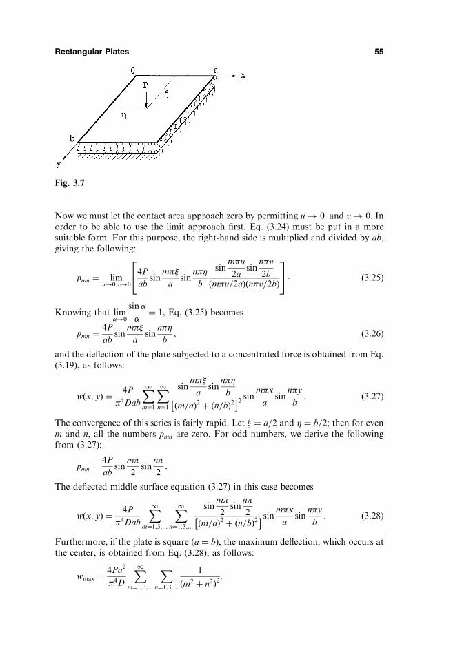
Now we must let the contact area approach zero by permitting u ! 0 and v ! 0. Inorder to be able to use the limit approach first, Eq. (3.24) must be put in a moresuitable form. For this purpose, the right-hand side is multiplied and divided by ab,giving the following:

pmn ¼ limu!0;v!0

4P

absin

m��

asin

n�

b

sinm�u

2asin

n�v

2bðm�u=2aÞðn�v=2bÞ

24

35 : ð3:25Þ

Knowing that lim!0

sin

¼ 1, Eq. (3.25) becomes

pmn ¼4P

absin

m��

asin

n�

b; ð3:26Þ

and the deflection of the plate subjected to a concentrated force is obtained from Eq.(3.19), as follows:

wðx; yÞ ¼ 4P

�4Dab

X1m¼1

X1n¼1

sinm��

asin

n�

b

ðm=aÞ2 þ ðn=bÞ2� �2 sinm�xa sinn�y

b: ð3:27Þ

The convergence of this series is fairly rapid. Let � ¼ a=2 and ¼ b=2; then for evenm and n, all the numbers pmn are zero. For odd numbers, we derive the followingfrom (3.27):

pmn ¼4P

absin

m�

2sin

n�

2:

The deflected middle surface equation (3.27) in this case becomes

wðx; yÞ ¼ 4P

�4Dab

X1m¼1;3;...

X1n¼1;3;...

sinm�

2sin

n�

2ðm=aÞ2 þ ðn=bÞ2� � sinm�x

asin

n�y

b: ð3:28Þ

Furthermore, if the plate is square (a ¼ b), the maximum deflection, which occurs atthe center, is obtained from Eq. (3.28), as follows:

wmax ¼4Pa2

�4D

X1m¼1;3;...

Xn¼1;3;...

1

ðm2 þ n2Þ2:


Fig. 3.7

Retaining the first nine terms of this series (m ¼ 1, n ¼ 1; 3; 5; m ¼ 3, n ¼ 1; 3; 5;m ¼ 5, n ¼ 1; 3; 5) we obtain

wmax ¼4Pa2

�4D

1

4þ 2

100þ 1

324þ 2

625þ 2

1156þ 1

2500

� �¼ 0:01142

Pa2

D:

The ‘‘exact’’ value is wmax ¼ 0:01159Pa2

Dand the error is thus 1.5% [3].

This very simple Navier’s solution, Eq. (3.28), converges sufficiently rapidly forcalculating the deflections. However, it is unsuitable for calculating the bendingmoments and stresses because the series for the second derivatives @2w=@x2 and@2w=@y2 obtained by differentiating the series (3.28) converge extremely slowly.These series for bending moment, and consequently for stresses as well as for theshear forces, diverge directly at a point of application of a concentrated force, calleda singular point. Thus, to calculate stress components in the vicinity of a concen-trated force, it is necessary to use a more efficient technique, especially since themaximum stresses occur in the immediate vicinity of the singular point. Therefore,the problem of determining a correct stress distribution near such types of singularpoints is of practical interest.

We now consider one approach for determining the bending moment distribu-tion near the above-mentioned singular point. Let us write the solution (3.27) in theform

w ¼ 4Pb3

�4a

X1m¼1

Sm sinm��

asin

m�x

a; ð3:29aÞ

where

Sm ¼ 1

2

X1n¼1

cosn�

bðy� Þ � cos

n�

bðyþ Þ

m2b2=a2 þ n2� �2 : ð3:29bÞ

The series (3.29b) can be summed using the formula [4]:

X1n¼1

cos nz

ð2 þ n2Þ2 ¼� 1

24þ �

43coshð�� zÞ

sin�� ð�� zÞ

42� sinh ð�� zÞ

sinh�

þ �2

42coshð�� zÞ cosh�

sin h2�:

ðaÞ

Using the above formula, we can represent the deflection surface (3.28) as

wðx; yÞ ¼ Pa2

�3D

X1m¼1

1þ m coth m � my1b

cothmy1b

� m b

cothm

b

� �

sinh

m

bsin h

my1b

sinm��

asin

m�x

am3 sinh m

;

ð3:30Þ

where m ¼ m�ba; y1 ¼ b� y; and y � . If y < , then the values y1 and must be

replaced by y and 1 ¼ b� , respectively.Let us use an infinitely long (in the y-direction) plate loaded by a concentrated

force P applied at x ¼ � and y ¼ 0, as shown in Fig. 3.8, to illustrate the above-

56 Chapter 3

mentioned approach. The deflection of such a plate-strip can be easily obtained fromEq. (3.30) by letting b ! 1. Then, taking into account the following approximateequalities,

tanh m � 1; cosh m � 1

2em ; sinh

mbðb� 2yÞ � cosh

mbðb� 2yÞ

� 1

2e m=bð Þ b�2yð Þ;

ð3:31Þ

we obtain the following expression for the deflection surface of the above-mentionedplate-strip:

w ¼ Pa2

2�3D

X1m¼1

1

m3sin

m��

asin

m�x

a1þm�y

a

� �e�

m�ya : ð3:32Þ

Differentiating the above expression twice in accordance with Eqs (2.13), we obtainthe following expressions for the bending moments

Mx ¼ P

2�

X1m¼1

1

msin

m��

asin

m�x

a1þ �þ ð1� �Þm�y

a

h ie�

m�ya ; ð3:33aÞ

My ¼P

2�

X1m¼1

1

msin

m��

asin

m�x

a1þ �� ð1� �Þm�y

a

h ie�

m�ya : ð3:33bÞ

Series in Eqs (3.33) can be summed up by using the formula [4]:

X1m¼1

1

msin

m�x

asin

m��

ae�

m�ya ¼ 1

4�lncosh

�y

a� cosh

�

aðxþ �Þ

cosh�y

a� cos

�

aðx� �Þ

: ð3:34Þ


Fig. 3.8

Let us present the equations for the bending and twisting moments for points thatare in the immediate vicinity from the point of application of force P but necessarilylying on the x axis. In this case, the values ðx� �Þ and y are very small and thefollowing approximate equalities hold:

cos�ðx� �Þ

a� 1� �

2ðx� �Þ22a2

; cosh�y

a� 1þ �2y2

2a2: ð3:35Þ

Applying the expression (3.34) and the above approximate equalities to Eqs (3.33),we obtain the following equations for the bending moments:

Mx

My

�¼ P

4�ð1þ �Þ ln

2a sin��

a�r

� ð1� �Þy2r2

8><>:

9>=>;; r2 ¼ ðx� �Þ2 þ y2: ð3:36Þ

As seen from Eqs (3.36), the bending moments and, consequently, shear forcesare unbounded at r ¼ 0, i.e., at a point where a concentrated force is applied. This isan evident reason of divergence of the Fourier series at the singular points. Anoccurrence of infinite stress resultants and stress couples can be physically explained.First, in reality there is no concentrated force. A load is always distributed over somefinite area. It can be easily shown that a finite value of a concentrated force cannotbalance the intensities of the shear forces and bending moments in the vicinity of apoint of application of P. Indeed, let us cut from the square plate subjected to acenter force P, a differential element of sides �x and �y surrounding this singularpoint (Fig. 3.9). Then, from a static equilibrium condition – namely, the forcesummation into the z direction is zero – we obtain

P� 2Qx�x� 2Qy�y ¼ 0;

58 Chapter 3

Fig. 3.9

w ¼ wh þ wp: ð3:40ÞConsider a plate with opposite edges, x ¼ 0 and x ¼ a, simply supported, and tworemaining opposite edges, y ¼ 0 and y ¼ b, which may have arbitrary supports.

The boundary conditions on the simply supported edges are

w ¼ 0jx¼0;x¼a and Mx ¼ �D@2w

@x2þ � @

2w

@y2

!¼ 0

x¼0;x¼a

: ð3:41aÞ

As mentioned earlier, the second boundary condition can be reduced to the follow-ing form:

@2w

@x2¼ 0

x¼0;x¼a

ð3:41bÞ

The complementary solution is taken to be

wh ¼X1m¼1

fmðyÞ sinm�x

a; ð3:42Þ

where fmðyÞ is a function of y only; wh also satisfies the simply supported boundaryconditions (3.41). Substituting (3.42) into the following homogeneous differentialequation

r2r2w ¼ 0 ð3:43Þgives

m�

a

� �4fmðyÞ � 2

m�

a

� �2d2fmðyÞdy2

þ d4fmðyÞdy4

" #sin

m�x

a¼ 0;

which is satisfied when the bracketed term is equal to zero. Thus,

d4fmðyÞdy4

� 2m�

a

� �2d2fmðyÞdy2

þ m�

a

� �4fmðyÞ ¼ 0 ð3:44Þ

The solution of this ordinary differential equation can be expressed as

fmðyÞ ¼ e�y: ð3:45ÞSubstituting the above into Eq. (3.44), gives the following characteristic equation:

�4 � 2m2�2

a2�2 þm4�4

a4¼ 0; ð3:46Þ

which has the two following two double roots

�1;2 ¼m�

a; �3;4 ¼ �m�

a: ð3:47Þ

According to the obtained values of the characteristic exponents, the solution of thehomogeneous equation can be expressed in terms of either exponential functions

fmðyÞ ¼ A 0me

m�y=a þ B 0me

�m�y=a þm�y

aC 0

mem�y=a þD 0

me�m�y=a

� � ð3:48Þ

or hyperbolic functions


fmðyÞ ¼ Am sinhm�y

aþ Bm cosh

m�y

aþm�y

aCm sinh

m�y

aþDm cosh

m�y

a

� �:

ð3:49Þ

The second form, Eq. (3.49), is more convenient for calculations.The complementary solution given by Eq. (3.42) becomes

wh ¼X1m¼1

Am sinhm�y

aþ Bm cosh

m�y

a

h

þm�y

aCm sinh

m�y

aþDm cosh

m�y

a

� �isin

m�x

a;

ð3:50Þ

where the constants Am;Bm;Cm; and Dm are obtained from the boundary conditionson the edges y ¼ 0 and y ¼ b:

The particular solution, wp, in Eq. (3.40), can also be expressed in a singleFourier series as

wpðx; yÞ ¼X1m¼1

gmðyÞ sinm�x

a: ð3:51Þ

The lateral distributed load pðx; yÞ is taken to be the following (see Appendix B):

pðx; yÞ ¼X1m¼1

pmðyÞ sinm�x

a; ð3:52Þ

where

pmðyÞ ¼2

a

ða0

pðx; yÞ sinm�xa

dx: ð3:53Þ

Substituting Eqs (3.51) and (3.52) into Eq. (3.44), gives

d4gmðyÞdy4

� 2m�

a

� �2d2gmðyÞdy2

þ m�

a

� �4gmðyÞ ¼

pmðyÞD

: ð3:54Þ

Solving this equation, we can determine gmðyÞ and, finally, find the particular solu-tion, wpðx; yÞ.

The complementary components of the stress resultants and stress couples,Mxh;Myh;Mxyh; and Vxh;Vyh; can be expressed in terms of fmðyÞ by substitutingEq. (3.50) into Eqs (2.13) and (2.39), as follows:

62 Chapter 3

where m ¼ m�b=2a.The deflection of the plate surface, Eq. (3.57a), may thus be expressed

w ¼ 4p0a4

�5D

X1m¼1;3;::

1

m51� m tanh m þ 2

2 coshmcosh

2my

bþ m2 cosh m

2y

b

�

sinh2my

b

�sin

m�x

a:

ð3:59Þ

The maximum deflection is obtained at the plate center (x ¼ a=2; y ¼ 0), where

wmax ¼4p0a

4

�5D

X1m¼1;3;...

ð�1Þm�12

m51� m tanh m þ 2

2 cosh m

� �:

Since

X1m¼1;3;...

ð�1Þm�12

m5¼ 5�5

29ð3Þ :

we can write the following expression for the maximum deflection of the plate:

wmax ¼5p0a

4

384D� 4p0a

4

�5D

X1m¼1;3;...

ð�1Þm�12 m tanh m þ 2ð Þ2 coshm m5

: ð3:60Þ

The first term above represents the deflection wmax of the middle of a uniformlyloaded, simply supported strip. The second term is a very rapidly converging series.For example, in the case of a square plate (a ¼ b and m ¼ m�=2), the maximumdeflection is given as

wmax ¼5p0a

4

384D� 4p0a

4

�5D0:68562� 0:00025 þ . . .ð Þ ¼ 0:00406

p0a4

D:

It is seen that the second term of the series in parentheses is negligible and that bytaking only the first term (m ¼ 1), the formula for deflection is obtained correct tothree significant figures.

Substituting the expression (3.57b) into the first and second equations (3.55),we obtain the following expressions for bending moments:

Mx ¼p0xða� xÞ

2þ ð1� �Þp0a2�2

X1m¼1;3;...

m2 Bm coshm�y

a

h

þCm

m�y

asinh

m�y

a� 2�

1� � coshm�y

a

� ��sin

m�x

a;

My ¼ �p0xða� xÞ

2� ð1� �Þp0a2�2

X1m¼1;3;...

m2 Bm coshm�y

a

h

þCm

m�y

asinh

m�y

aþ 2

1� � coshm�y

a

� ��sin

m�x

a;

ð3:61Þ

where Bm and Cm are given by Eqs (e).Both series in Eqs (3.61) converge rapidly. At the center (x ¼ a=2; y ¼ 0) of the

square plate the bending moments are given as


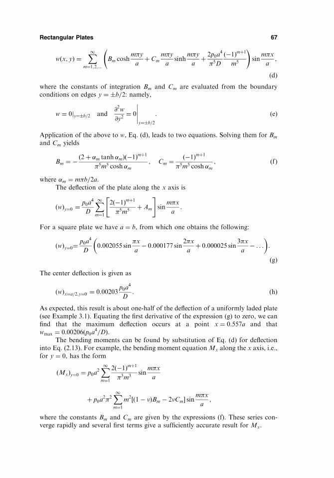
wðx; yÞ ¼X1

m¼1;2;...

Bm coshm�y

aþ Cm

m�y

asinh

m�y

aþ 2p0a

4

�5D

ð�1Þmþ1

m5

!sin

m�x

a;

ðdÞwhere the constants of integration Bm and Cm are evaluated from the boundaryconditions on edges y ¼ �b=2: namely,

w ¼ 0jy¼�b=2 and@2w

@y2¼ 0

y¼�b=2

: ðeÞ

Application of the above to w, Eq. (d), leads to two equations. Solving them for Bm

and Cm yields

Bm ¼ � 2þ m tanh mð Þ �1ð Þmþ1

�5m5 cosh m; Cm ¼ �1ð Þmþ1

�5m5 cosh m; ðfÞ

where m ¼ m�b=2a.The deflection of the plate along the x axis is

wð Þy¼0 ¼ p0a4

D

X1m¼1

2 �1ð Þmþ1

�5m5þ Am

" #sin

m�x

a:

For a square plate we have a ¼ b, from which one obtains the following:

wð Þy¼0¼p0a

4

D0:002055 sin

�x

a� 0:000177 sin

2�x

aþ 0:000025 sin

3�x

a� . . .

� �:

ðgÞThe center deflection is given as

wð Þx¼a=2;y¼0 ¼ 0:00203p0a

4

D: ðhÞ

As expected, this result is about one-half of the deflection of a uniformly laded plate(see Example 3.1). Equating the first derivative of the expression (g) to zero, we canfind that the maximum deflection occurs at a point x ¼ 0:557a and thatwmax ¼ 0:00206ðp0a4=DÞ.

The bending moments can be found by substitution of Eq. (d) for deflectioninto Eq. (2.13). For example, the bending moment equation Mx along the x axis, i.e.,for y ¼ 0, has the form

Mxð Þy¼0 ¼ p0a2X1m¼1

2ð�1Þmþ1

�3m3sin

m�x

a

þ p0a2�2

X1m¼1

m2 ð1� �ÞBm � 2�Cm½ � sinm�xa;

where the constants Bm and Cm are given by the expressions (f). These series con-verge rapidly and several first terms give a sufficiently accurate result for Mx:


Example 3.5

Derive expressions for the deflected surface and the bending moments in a floorplate-strip subjected to a uniformly distributed load q0 along line y ¼ 0, as shownin Fig. 3.12a. Assume the edges x ¼ 0 and x ¼ a are simply supported.

Solution

If a plate is strongly lengthened in one direction – for example, in the y direction –then such a plate in some problems can be considered as an infinite one in thisdirection. Levy’s solution can be applied advantageously with some modificationsto obtain the expressions for the deflections and bending moments.

The solution of the governing differential equation (2.24) is sought in the formof Eq. (3.48). At the same time, since for y ! 1 deflections cannot approach infi-nity, then the terms containing em�y=a should be equated to zero because these termsand their derivatives do not vanish at y ! 1. Hence, wh can be represented asfollows:

wh ¼X1m¼1

B 0m þm�y

aD 0

m

� �e�m�y=a sin

m�x

a: ðaÞ

The above satisfies Eq. (2.24) and the boundary conditions on the edges x ¼ 0 andx ¼ a.

Let us consider the lower part of the plate where y � 0. The constants B 0m and

D 0m can be evaluated from the conditions of symmetry of the plate and loading at

y ¼ 0. First, due to the symmetry of the deflected middle surface of the plate withrespect to the x axis, the derivative @w=@y is zero at y ¼ 0; this condition is satisfied ifB 0m ¼ D 0

m. Therefore, Eq. (a) becomes (for the lower part of the plate)

68 Chapter 3

Fig. 3.12

w in the form of Eq. (b) satisfies Eq. (3.43) and the boundary conditions (d) exactly.Using the relations (2.12) and Eq. (a), the boundary conditions (c) can be rewritten,as follows

w ¼ 0jx¼0;a; �D@2w

@x2þ � @

2w

@y2

!" #x¼0

¼ Fn sin ny and@2w

@x2þ � @

2w

@y2

!x¼a

¼ 0:

ðeÞSubstitution of Eqs (b) into (e) and solving the obtained equations for Cin, oneobtains

C1n ¼ 0;C2n ¼ � Fn

2D;C3n ¼

Fn

2D1� coth2 na� �

na;C4n ¼Fn

2Dcothna: ðfÞ

Inserting the above into Eq. (f) yields the following:

w ¼X1n¼1

Fn

2D2n sinh nanx cosh nða� xÞ � na

sinh nx

sinh na

� �sin ny: ð3:62Þ

As it follows from the above, in order to obtain a particular solution for platessubjected to various types of load distribution pðx; yÞ ¼ p0 � f ðxÞ it is necessary todetermine the coefficients pm (see Eq. (3.53)). Table 3.2 furnishes the values of pm forvarious types of load distributions.

3.6 CONTINUOUS PLATES

When a uniform plate extends over a support and has more than one span along itslength or width, it is termed continuous. Such plates are of considerable practicalinterest.

Continuous plates are externally statically indeterminate members (note that aplate itself is also internally statically indeterminate). So, the well-known methodsdeveloped in structural mechanics can be used for the analysis of continuous plates.In this section, we consider the force method which is commonly used for the analysisof statically indeterminate systems. According to this method, the continuous plate issubdivided into individual, simple-span panels between intermediate supports byremoving all redundant restraints. It can be established, for example, by introducingsome fictitious hinges above the intermediate supports. In this way, the redundantmoments acting along the intermediate supports are eliminated. Similar fictitioushinges can be used at the ends if those are fixed. The simple-span panel obtainedin such a way is referred to as a primary plate. In order to restore the rejectedrestraints, the unknown redundant moments are applied to the primary plate.These moments can be determined from the solution of simultaneous algebraicequations expressing the compatibility of the slopes between the adjoining panelsproduced by both external loads and unknown redundant moments.

In our further discussion we assume that the supports are unyielding. For thesake of simplicity, we confine ourselves to a rectangular plate continuous in onedirection only and having the same flexural rigidity. Obviously, the general proce-dure of the force method discussed below can be applied to plates continuous in bothdirections.


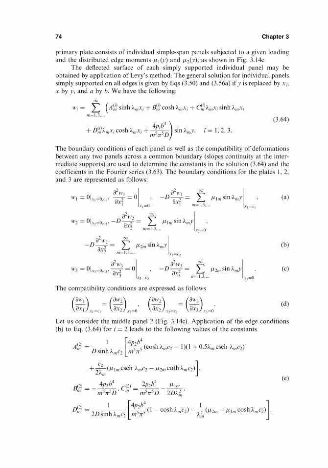
primary plate consists of individual simple-span panels subjected to a given loadingand the distributed edge moments �1ðyÞ and �2ðyÞ, as shown in Fig. 3.14c.

The deflected surface of each simply supported individual panel may beobtained by application of Levy’s method. The general solution for individual panelssimply supported on all edges is given by Eqs (3.50) and (3.56a) if y is replaced by xi,x by y, and a by b. We have the following:

wi ¼X1

m¼1;3;...

AðiÞm sinh �mxi þ BðiÞ

m cosh �mxi þ CðiÞm �mxi sinh �mxi

�

þDðiÞm �mxi cosh �mxi þ

4pib4

m5�5D

!sin �my; i ¼ 1; 2; 3:

ð3:64Þ

The boundary conditions of each panel as well as the compatibility of deformationsbetween any two panels across a common boundary (slopes continuity at the inter-mediate supports) are used to determine the constants in the solution (3.64) and thecoefficients in the Fourier series (3.63). The boundary conditions for the plates 1, 2,and 3 are represented as follows:

w1 ¼ 0jx1¼0;c1 ;@2w1

@x21¼ 0

x1¼0

; �D@2w1

@x21¼

X1m¼1;3;...

�1m sin �my

x1¼c1

; ðaÞ

w2 ¼ 0jx2¼0;c2 ;�D@2w2

@x22¼

X1m¼1;3;...

�1m sin �my

x2¼0

;

�D@2w2

@x22¼

X1m¼1;3;...

�2m sin �my

x2¼c2

ðbÞ

w3 ¼ 0jx3¼0;c3 ;@2w3

@x23¼ 0

x3¼c3

; �D@2w3

@x23¼

X1m¼1;3;...

�2m sin �my

x3¼0

: ðcÞ

The compatibility conditions are expressed as follows

@w1

@x1

� �x1¼c1

¼ @w2

@x2

� �x2¼0

;@w2

@x2

� �x2¼c2

¼ @w3

@x3

� �x3¼0

: ðdÞ

Let us consider the middle panel 2 (Fig. 3.14c). Application of the edge conditions(b) to Eq. (3.64) for i ¼ 2 leads to the following values of the constants

Að2Þm ¼ 1

D sinh �mc2

4p2b4

m5�5cosh �mc2 � 1ð Þ 1þ 0:5�m csch �mc2ð Þ

"

þ c22�m

�1m csch �mc2 � �2m coth �mc2ð Þ�;

Bð2Þm ¼ � 4p2b

4

m5�5D;Cð2Þ

m ¼ 2p2b4

m5�5D� �1m

2D�2m;

Dð2Þm ¼ 1

2D sinh �mc2

4p2b4

m5�51� cosh �mc2ð Þ � 1

�2m�2m � �1m cosh �mc2ð Þ

" #:

ðeÞ

74 Chapter 3

which substituted into Eq. (3.15a) yields

wðx; yÞ ¼X1n¼1

X1m¼1

pmn sinm�x

asin

n�y

b

D�4 m2=a2 þ n2=b2� �2þk

: ð3:69Þ

If a plate is subjected to a uniform load of intensity p0, then Eq. (3.69) becomes

w ¼ 16p0�2

X1n¼1

X1m¼1

sinm�x

asin

n�y

b

mn �4Dðm2=a2 þ n2=b2Þ2 þ k� �: ð3:70Þ

If a plate is loaded by a concentrated force P applied at a point (�; ), then thedeflected surface equation of the plate can be represented by the following form:

w ¼ 4P

ab

X1n¼1

X1m¼1

sinm��

asin

n�

b�4Dðm2=a2 þ n2=b2Þ2 þ k

sinm�x

asin

n�y

b: ð3:71Þ

Having the deflection of the plate produced by a concentrated force, the deflectionproduced by any kind of lateral loading is obtained by the method of superposition.

3.7.2 Application of Levy’s method

If any two opposite edges of the plate on an elastic foundation are simply supported,say, the edges x ¼ 0 and x ¼ a, then Levy’s solution presented earlier in Sec. 3.5 canbe applied advantageously. The general solution of the governing differential equa-tion of the plate on an elastic foundation, Eq. (3.67), may be represented again in theform of the sum of particular and complementary solutions, i.e.,

w ¼ wp þ wh: ð3:72ÞExpressing the complementary solution by the Fourier series, yields

wh ¼X1m¼1

fmðyÞ sinm�x

a: ð3:73Þ

Substituting the above into the homogeneous part of Eq. (3.66) and solving it forfmðyÞ, we obtain

fmðyÞ ¼ Am sinh my sin myþ Bm sinh my cosmyþ Cm cosh my sin my

þDm coshmy cosmy;

ð3:74Þwhere

m ¼

ffiffiffiffiffiffiffiffiffiffiffiffiffiffiffiffiffiffiffiffiffiffiffiffiffiffiffiffiffiffiffiffiffiffiffiffiffiffiffiffiffiffiffiffiffiffiffiffiffiffiffi1

2

m2�2

a2þ

ffiffiffiffiffiffiffiffiffiffiffiffiffiffiffiffiffiffiffiffim4�4

a4þ k

D

s0@

1A

vuuut ; m ¼

ffiffiffiffiffiffiffiffiffiffiffiffiffiffiffiffiffiffiffiffiffiffiffiffiffiffiffiffiffiffiffiffiffiffiffiffiffiffiffiffiffiffiffiffiffiffiffiffiffiffiffiffiffiffiffiffi1

2�m2�2

a2þ

ffiffiffiffiffiffiffiffiffiffiffiffiffiffiffiffiffiffiffiffim4�4

a4þ k

D

s0@

1A

vuuut :

ð3:75ÞSubstituting (3.74) into (3.73), we can obtain the expression for complementarysolution wh. Similarly, if we express the particular solution as

78 Chapter 3

wp ¼X1m¼1

gmðyÞ sinm�x

a; ð3:76Þ

and the applied load as

p ¼X1m¼1

pmðyÞ sinm�x

a; ð3:77Þ

and then we substitute these equations into Eq. (3.66), we obtain

d4gmdy4

� 2m�

a

� �2d2gmdy2

þ m4�4

a4þ k

D

!gm ¼ pmðyÞ

D: ð3:78Þ

Solving Eq. (3.78) for gm, we can find the particular solution wp. Therefore, Eq.(3.76) together with Eqs (3.73) and (3.74) describes the deflected surface of the plate.

Example 3.8

Find the equation for the deflection of a rectangular plate, resting on a Winklerfoundation of modulus k and subjected to a uniform loading of intensity p0. Assumethat edges x ¼ 0 and x ¼ a are simply supported while edges y ¼ �b=2 are fixed.

Solution

For a uniform loading p, the right-hand side of Eq. (3.66) is constant. Thus, theparticular solution is also a constant and may be taken in the following form:

gm ¼ B; ðaÞand the expression for pm is given by (see Table 3.2)

pm ¼ 4p0m�

: ðbÞ

Substitution of (a) and (b) into Eq. (3.78) results in the following particular solution:

gm ¼ 4p0Dm�

1

m4�4

a4þ kD

� � : ðcÞ

Due to the symmetry of the deflection around the x axis, we can take Bm ¼ Cm ¼ 0in Eq. (3.74) and the general solution for deflection becomes

w ¼X1m¼1

Am sinh my sin myþDm cosh my cosmyþ gmð Þ sinm�xa; ð3:79Þ

where Am and Bmare constants of integration. They have to be evaluated from theboundary conditions on the edges y ¼ �b=2; namely,

w ¼ 0jy¼�b=2;@w

@y¼ 0

y¼�b=2

: ðdÞ

Substituting the expressions (3.79) into these boundary conditions, gives


arbitrary reaction load qðx; yÞ occurring over a plate base causes the followingdeflection at point ðxi; yiÞ:

wðxi; yiÞ ¼ða0

ðb0

K ðx� xiÞ; ðy� yiÞ½ �qðx; yÞdxdy: ð3:80Þ

The above-mentioned function K ½. . .� is given by the following [13]:

K ½. . .� ¼ 1� �2�E

1

r; ð3:81Þ

where r is the distance between the point of load application ðx; yÞ and point ofobservation (xi; yi), r

2 ¼ ðx� xiÞ2 þ ðy� yiÞ2. With regard to expression (3.81) andreplacing a unit force by qdxdy, Eq. (3.80) may be rewritten as

wðxi; yiÞ ¼1� �2�E

ða0

ðb0

qðx; yÞdxdyffiffiffiffiffiffiffiffiffiffiffiffiffiffiffiffiffiffiffiffiffiffiffiffiffiffiffiffiffiffiffiffiffiffiffiffiffiffiffiffiffiðx� xiÞ2 þ ðy� yiÞ2

q : ð3:82Þ

For this model, the relationship between the deflection of the foundation w and thefoundation reaction q is much more complicated than for the Winkler model. Thus,the problem of bending of a plate resting on a semi-infinite space becomes moredifficult. In the majority of cases, such plate bending problems can be solved numeri-cally only.

3.8 PLATES WITH VARIABLE STIFFNESS

Let us consider bending of a rectangular plate having a variable thickness,h ¼ hðx; yÞ. We assume that the above thickness varies gradually and there is noabrupt variation in thickness so that the expressions for the bending and twistingmoments derived earlier for plates of constant thickness, Eqs (2.13), apply withsufficient accuracy to this case also. Substituting the above equations for the bendingand twisting moments into the equation of static equilibrium (2.23) and taking intoaccount that D ¼ Dðx; yÞ. One obtains the following:

Dr2r2wþ 2@D

@x

@

@xðr2wÞ þ 2

@D

@y

@

@yðr2wÞ þ r2Dðr2wÞ

� ð1� �Þ @2D

@x2@2w

@y2� 2

@2D

@x@y

@2w

@x@yþ @

2D

@y2@2w

@x2

!¼ p:

ð3:83Þ

This is the governing fourth-order partial differential equation with variable coeffi-cients in w describing the bending of thin plates with variable thickness. A closed-form solution of this equation is possible in very special cases only. Practically, platesof variable thickness can be treated by approximate and numerical methods intro-duced in Chapter 6. Among them, the variational (the Ritz method) and finiteelement methods are widely used in practice. Analysis of plates with variable thick-ness can be efficiently carried out by the small parameter method [3]. Let us illustratean application of this method to rectangular plates of variable stiffness.


For simplicity, assume that the plate stiffness varies in one direction only, say,in the y direction. So, the plate thickness, h, varies according to the law

h ¼ h0 1þ ��ðyÞ½ �; ð3:84Þwhere � is a constant and is in the range 0 < � < 1, �ðyÞ is a given function describ-ing a variation of the plate thickness over the y cordinate, and h0 is some referenceplate thickness.

Thus,

D ¼ E hðyÞ½ �312ð1� �2Þ ¼ D0 1þ ��ðyÞ½ �3; D0 ¼

Eh3012ð1� �2Þ : ð3:85Þ

The small parameter method introduces the value � as a parameter of a solution ofthe given problem. Considering the deflection as a function of x; y; and �, representwðx; y; �) in the form

w ¼X1m¼0

wm�m; ð3:86Þ

where wm ¼ wmðx; yÞ: Substituting the expressions (3.85) and (3.86) into Eq. (3.83)and equating the coefficients for identical powers of � to zero, we obtain the follow-ing sequence of differential equations:

r2r2w0 ¼p

D0

;

r2r2w1 ¼ �3 �ðyÞr2r2w0 þ 2� 0ðyÞ @@y

r2w0 þ� 00ðyÞ r2w0 � ð1� �Þ @2w0

@x2

" #( );

r2r2w2 ¼ �3 �ðyÞr2r2w1 þ 2� 0ðyÞ @@y

r2w1 þ� 00ðyÞ r2w1 � ð1� �Þ @2w1

@x2

" #( )

� 3 �ðyÞ½ �2r2r2w0 þ 4�ðyÞ� 0ðyÞ @@y

r2w0 þ 2

� 0ðyÞ� �2þ�ðyÞ� 00ðyÞh i

r2w0 � ð1� �Þ @2w0

@x2

" #);

etc:

ð3:87Þ

where the prime notations indicate the derivatives of the function �ðyÞ with respectto y. Assume for simplicity that the plate edges x ¼ 0 and x ¼ a are simply sup-ported. Then, following the Levy method, solutions of Eqs (3.87) are sought in theform of the following series:

82 Chapter 3

w0 ¼X1n¼1

w0n sinn�x

a;

w1 ¼X1n¼1

w1n sinn�x

a;

w2 ¼X1n¼1

w2n sinn�x

a

etc . . . . . . . . . . . . . . .

ð3:88Þ

where the coefficients wmn ðm ¼ 0; 1; 2; . . .Þ are functions of the y only. Expand thegiven loading in the series also, as follows:

pðx; yÞ ¼X1n¼1

pnðyÞ sinn�x

a: ð3:89Þ

Substituting the first expression (3.88) and Eq. (3.89) into the first equation (3.87)and satisfying the boundary conditions prescribed on the plate edges y ¼ 0 andy ¼ b, we can determine w0n. Then, substitution of the first and second expressions(3.88) into the second equation (3.87) gives w1n. Similarly, each of the functions wm

can be found by substitution of w0;w1; . . . ;wm�1 into the corresponding differentialequation of the system (3.87) involving wm into the left-hand side. Finally, thedeflection surface of the plate is obtained by substituting for w0;w1;w2; . . . ;wm

from Eqs (3.88) into Eq. (3.86). The interested reader can find an application ofthis and other methods to plates of variable thickness in Ref. [14].

Example 3.9

A rectangular plate of variable thickness in the y direction is simply supported onedges x ¼ 0 and x ¼ a and is fixed on edges y ¼ 0 and y ¼ b. The plate thicknessvaries according to the law h ¼ h0ð1þ �yÞ. The plate is subjected to a loadp ¼ p0 sin

n�xasin m�y

b. Find the deflections and bending moments in the plate.

Solution

This problem was solved numerically by using the above-presented general proce-dure of the small-parameter method. The boundary conditions are found to be asfollows:

w ¼ @2w

@x2¼ 0

x¼0;a

;w ¼ @w

@y¼ 0

y¼0;b

:

For the plate under consideration, �ðyÞ � y. The values of the deflection and bend-ing moment My at a plate section x ¼ a=2 are given in Table 3.3. These results wereobtained by using the three terms in the expansion (3.86) for a plate with the follow-ing geometric and mechanical parameters: a ¼ b ¼ 1m; h0 ¼ 0:0625m; � ¼ 0:5; and� ¼ 0:3.


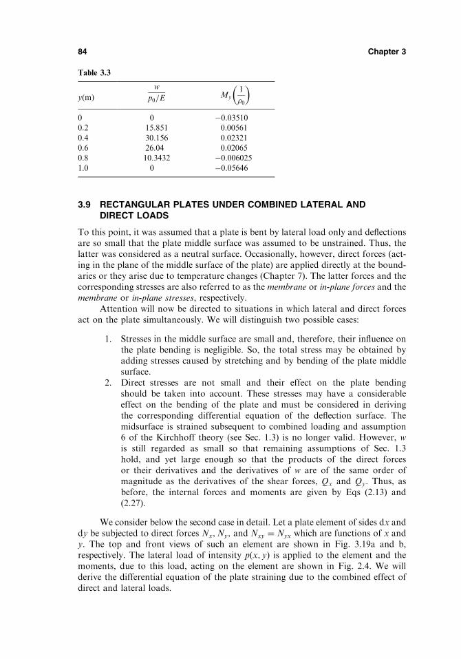
3.9 RECTANGULAR PLATES UNDER COMBINED LATERAL ANDDIRECT LOADS

To this point, it was assumed that a plate is bent by lateral load only and deflectionsare so small that the plate middle surface was assumed to be unstrained. Thus, thelatter was considered as a neutral surface. Occasionally, however, direct forces (act-ing in the plane of the middle surface of the plate) are applied directly at the bound-aries or they arise due to temperature changes (Chapter 7). The latter forces and thecorresponding stresses are also referred to as the membrane or in-plane forces and themembrane or in-plane stresses, respectively.

Attention will now be directed to situations in which lateral and direct forcesact on the plate simultaneously. We will distinguish two possible cases:

1. Stresses in the middle surface are small and, therefore, their influence onthe plate bending is negligible. So, the total stress may be obtained byadding stresses caused by stretching and by bending of the plate middlesurface.

2. Direct stresses are not small and their effect on the plate bendingshould be taken into account. These stresses may have a considerableeffect on the bending of the plate and must be considered in derivingthe corresponding differential equation of the deflection surface. Themidsurface is strained subsequent to combined loading and assumption6 of the Kirchhoff theory (see Sec. 1.3) is no longer valid. However, wis still regarded as small so that remaining assumptions of Sec. 1.3hold, and yet large enough so that the products of the direct forcesor their derivatives and the derivatives of w are of the same order ofmagnitude as the derivatives of the shear forces, Qx and Qy. Thus, asbefore, the internal forces and moments are given by Eqs (2.13) and(2.27).

We consider below the second case in detail. Let a plate element of sides dx anddy be subjected to direct forces Nx;Ny; and Nxy ¼ Nyx which are functions of x andy. The top and front views of such an element are shown in Fig. 3.19a and b,respectively. The lateral load of intensity pðx; yÞ is applied to the element and themoments, due to this load, acting on the element are shown in Fig. 2.4. We willderive the differential equation of the plate straining due to the combined effect ofdirect and lateral loads.

84 Chapter 3

Table 3.3

yðmÞw

p0=EMy

1

�0

� �

0 0 �0:035100.2 15.851 0.00561

0.4 30.156 0.02321

0.6 26.04 0.02065

0.8 10.3432 �0:0060251.0 0 �0:05646

Consider the equilibrium of the element shown in Fig. 3.19, which is subjectedto the in-plane forces Nx;Ny; and Nxy, as well as to the lateral load pðx; yÞ. First, weapply the condition

PFx ¼ 0. Referring to Fig. 3.19a, from the equilibrium of Nxdy

forces into the x-direction, we obtain the following:

Nx þ@Nx

@xdx

� �dy cos 0 �Nxdy cos; ðaÞ

where 0 ¼ þ d ¼ þ @@x dx. Noting that deflections are assumed to be very small

and, hence, for small cos � 1, and that likewise, cos 0 � 1, Eq. (a) reduces to@Nx

@x dxdy. The sum of the x components of Nxydx is treated in a similar way. Thus,the force summation in the x direction leads to

@Nx

@xþ @Nxy

@y¼ 0: ð3:90aÞ

Furthermore, the conditionP

Fy ¼ 0 results in the following:

@Nxy

@xþ @Ny

@y¼ 0: ð3:90bÞ

Equations (3.90) are independent from the equilibrium equations of Sec. 2.3 and maybe studied separately.

Considering the projection of all the forces (direct and lateral) on the z axis, theplate deflection must be taken into account. Due to the bending of the plate in the xzplane, the z component of the normal force Nx is equal to (Fig. 3.19b)

�Nxdy sin þ Nx þ@Nx

@xdx

� �dy sin 0 ðbÞ

Inasmuch as and 0 are small, sin � � @w=@x and sin 0 � 0, where 0 ¼ þ d. The latter can be represented as

0 � þ @@x

dx ¼ @w

@xþ @

2w

@x2dx;


Fig. 3.19

Example 3.10

A rectangular plate with simply supported edges is subjected to the action of acombined uniform lateral load p and uniform tension N as shown in Fig. 3.20.Derive the equation of the deflection surface.

Solution

The lateral load p can be represented by the double trigonometric series (Eq. (a) ofExample 3.1)

p ¼ 16p0�2

X1m¼1;3;5;...

X1n¼1;3;5;...

1

mnsin

m�x

asin

n�y

b: ðaÞ

Inserting the above into Eq. (3.92), we obtain the following (letting Nx ¼ N):

@4w

@x4þ 2

@4w

@x2@y2þ @

4w

@y4�N

D

@2w

@x2¼ 16p0

�2

X1m¼1;3;5;...

X1n¼1;3;5;...

1

mnsin

m�x

asin

n�y

b: ðbÞ

The boundary conditions of a simply supported plate will be satisfied if we take thedeflection w in the form of series

w ¼Xm

Xn

wmn sinm�x

asin

n�y

b: ðcÞ

Substituting this series into Eq. (b), we find the following values for coefficients wmn:

wmn ¼16p0

D�6mn m2=a2 þ n2=b2� �2þ Nm2

�2Da2

" # ; m; n ¼ 1; 3; 5; . . . : ðdÞ

Hence, the deflection surface of the plate is given by


Fig. 3.20

w ¼ 16p0�6D

X1m¼1;3;5;...

X1n¼1;3;5;...

sinm�x

asin

n�y

b

mn m2=a2 þ n2=b2� �2þ Nm2

�2Da2

" #: ðeÞ

Comparing this result with the solution (3.21a), we conclude from the presence of theterm Nm2=�2Da2 in the brackets of the denominator that the deflection of the plate issomewhat diminished by the action of the tensile forces N. This is as would beexpected.

3.10 BENDING OF PLATES WITH SMALL INITIAL CURVATURE

Let us assume that a plate has an initial curvature of its middle surface, i.e., there isan initial deflection w0 at any point of the above surface. It is assumed that w0 issmall compared with the plate thickness. If the plate is subject to lateral load andthen an additional deflection w1 occurs, the total deflection is thus

w ¼ w0 þ w1: ð3:93ÞHere w1 is the solution of Eq. (2.24) set up for the flat plate, i.e., without the above-mentioned initial deflection. It will be valid if the small initial deflection, w0, isconsidered as a result of the action of some fictitious lateral load. Then, applyingthe superposition principle (recall that the above principle cannot be applied forlarge deflections), it is possible to determine the total deflection.

If besides the lateral load, the direct forces are also applied to an initiallycurved plate, then these forces produce bending also, which depends not only onw1 but also on w0. In order to determine the total deflection, w, we introduce w ¼w0 þ w1 into the right hand side of Eq. (3.92). The left-hand side of this equationtakes into account a change in curvature from the initial curved state due to thegiven lateral load. Therefore, w1 has to be substituted for w on the left-hand sideof Eq. (3.92). Thus, Eq. (3.92) for the initially curved plate is of the followingform:

@4w1

@x4þ 2

@4w1

@x2@y2þ @

4w1

@y4¼ 1

DpþNx

@2ðw0 þ w1Þ@x2

þNy

@2ðw0 þ w1Þ@y2

"

þ2Nxy

@2ðw0 þ w1Þ@x@y

#:

ð3:94Þ

As mentioned previously, the influence of the initial curvature on the total deflectionof the plate is equivalent to the influence of some fictitious lateral load of intensity pfequal to

pf ¼ Nx

@2w0

@x2þNy

@2w0

@y2þ 2Nxy

@2w0

@x@y: ð3:95Þ

Hence, an initially curved plate will experience a bending under action of the directforces, lying in the plate middle surface only.

88 Chapter 3

Example 3.11

Consider a simply supported plate with sides a and b. Assume that the initial deflec-tion is defined by the following equation:

w0 ¼ 11 sin�x

asin�y

b: ðaÞ

The plate edges x ¼ 0 and x ¼ a are subjected to an in-plane uniform compressiveforce Nx ¼ �N, as shown in Fig. 3.21. Find the deflected surface of the plate.

Solution

The differential equation (3.94) together with Eq. (a) will take the following form forthe problem under consideration:

@4w1

@x4þ 2

@4w1

@x2@y2þ @

4w1

@y4¼ N

D

11�2

a2sin�x

asin�y

b� @

2w1

@x2

!: ðbÞ

Let us represent a solution of the above equation in the form

w1 ¼ A sin�x

asin�y

b; ðcÞ

where A is unknown parameter. This solution satisfies exactly the simply supportedboundary conditions. Inserting Eq. (c) into Eq. (b) yields

A ¼ 11N

�2Da2

1þ a2

b2

� �2

�N

: ðdÞ

Substituting for A from Eq. (d) into Eq. (c), one obtains the deflection w1, caused bythe compressive forces N. Adding this deflection to the initial deflection (a), gives thefollowing total deflection of the plate:

w ¼ w0 þ w1 ¼111� sin

�x

asin�y

b; ðeÞ


Fig. 3.21

where

¼ N

�2Da2

1þ a2

b2

� �2: ðfÞ

The maximum deflection occurs at the plate center. Setting x ¼ a=2 and y ¼ b=2, weobtain

wmax ¼111� : ðgÞ

In general case, a given initial deflection of the plate can be expanded into thefollowing Fourier series:

w0 ¼X1

m¼1;3;...

X1n¼1;3;...

mn sinm�x

asin

n�y

bðhÞ

Substituting the above into Eq. (b) and solving yields

w1 ¼X1

m¼1;3;...

X1n¼1;3;...

bmn sinm�x

asin

n�y

b; ðiÞ

where

bmn ¼mnN

�2Da2

mþ n2a2

m2b2

� �2

�N

: ðkÞ

As follows from Eq. (k), the coefficients bmn are increased with an increase of theforce N.

To write the equation for a plate subjected to initial deflection and to in-planeuniform tensile forces, it is required to change the sign of N in Eq. (b) of the fore-going example only. By following the approach described above, the deflection of aninitially curved plate subjected to a simultaneous action of in-plane forces Nx;Ny;and Nxymay also be readily obtained.

PROBLEMS

3.1 A rectangular plate with sides a and b (0 � x � a, 0 � y � b) is bent according to the

following equation w ¼ C sin�x=a sin�y=b. Clarify the type of loading and static

boundary conditions that correspond to the given deflection surface.

3.2 Given the deflection surface of the rectangular plate with sides a and b (0 � x � a,

0 � y � b) in the form w ¼ Axyðx� aÞðy� bÞ, specify the type of loading and kine-

matic boundary conditions corresponding to the given deflection surface of the plate.

3.3 A square plate is subjected to uniformly distributed twisting moments Mxy ¼ Myx

applied to all its four edges. Determine the expression for the deflection surface.

3.4 Formulate the conditions under which a cylindrical bending can occur.

3.5 A rectangular plate of sides a and b is subjected to uniformly distributed bending

moments m applied to all four edges of the plate (see Fig. 3.2, where m1 ¼ m2 ¼ m).

Its curved middle surface should present a portion of a sphere because the radii of

curvature are identical in all planes and at all points of the plate. However, as follows

90 Chapter 3

4

Circular Plates

4.1 INTRODUCTION

Circular plates are common in many structures such as nozzle covers, end closures inpressure vessels, pump diaphragms, turbine disks, and bulkheads in submarines andairplanes, etc. When circular plates are analyzed, it is convenient to express thegoverning differential equation (2.24) in polar coordinates. This can be readilyaccomplished by a coordinate transformation. An alternative approach based onthe procedure presented in Chapter 3 for rectangular plates to derive the basicrelationships for the lateral deflections of circular plates may be used also.

4.2 BASIC RELATIONS IN POLAR COORDINATES

As mentioned earlier, we use the polar coordinates r and ’ in solving the bendingproblems for circular plates. If the coordinate transformation technique is used, thefollowing geometrical relations between the Cartesian and polar coordinates areapplicable (see Fig. 4.1a):

x ¼ r cos ’; y ¼ r sin ’ and r2 ¼ x2 þ y2; ’ ¼ tan�1 y

x: ð4:1Þ

Referring to the above

@r

@x¼ x

r¼ cos ’;

@r

@y¼ y

r¼ sin ’;

@’

@x¼ � y

r2¼ � sin ’

r;

@’

@y¼ x

r2¼ cos ’

r:

ð4:2Þ

Inasmuch as the deflection is a function of r and ’, the chain rule together with therelations (4.2) lead to the following

95

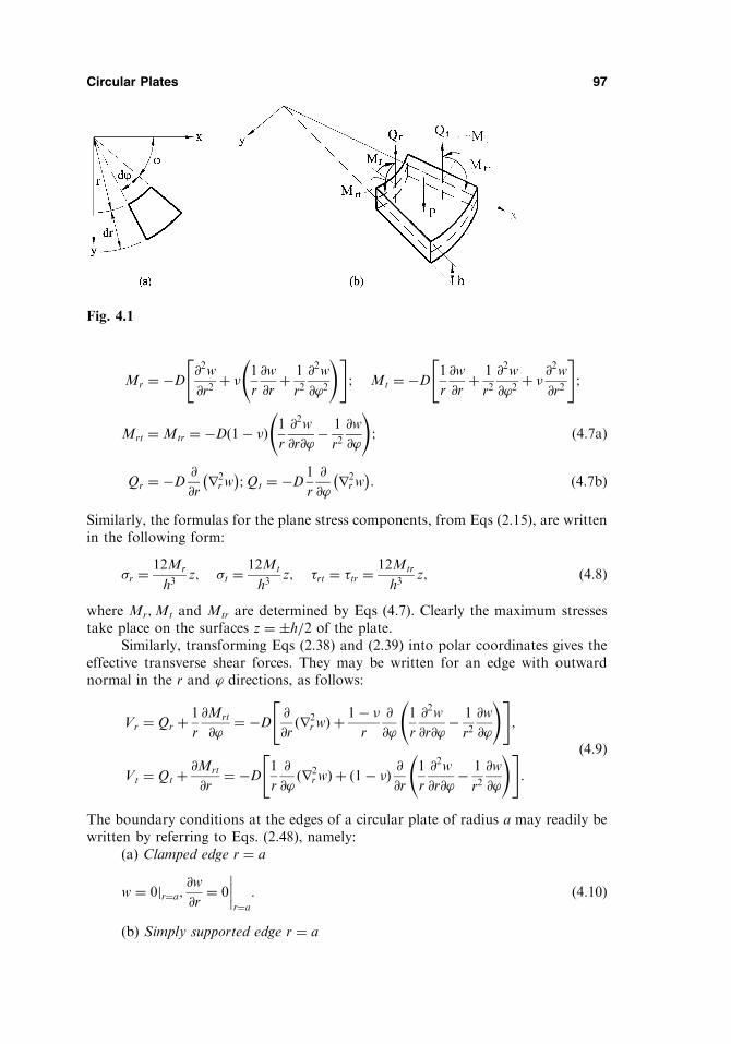
Mr ¼ �D@2w

@r2þ � 1

r

@w

@rþ 1

r2@2w

@’2

!" #; Mt ¼ �D

1

r

@w

@rþ 1

r2@2w

@’2þ � @

2w

@r2

" #;

Mrt ¼ Mtr ¼ �Dð1� �Þ 1

r

@2w

@r@’� 1

r2@w

@’

!; ð4:7aÞ

Qr ¼ �D@

@rr2r w

� �;Qt ¼ �D

1

r

@

@’r2r w

� �: ð4:7bÞ

Similarly, the formulas for the plane stress components, from Eqs (2.15), are writtenin the following form:

�r ¼12Mr

h3z; �t ¼

12Mt

h3z; �rt ¼ �tr ¼

12Mtr

h3z; ð4:8Þ

where Mr;Mt and Mtr are determined by Eqs (4.7). Clearly the maximum stressestake place on the surfaces z ¼ �h=2 of the plate.

Similarly, transforming Eqs (2.38) and (2.39) into polar coordinates gives theeffective transverse shear forces. They may be written for an edge with outwardnormal in the r and ’ directions, as follows:

Vr ¼ Qr þ1

r

@Mrt

@’¼ �D

@

@rðr2

r wÞ þ1� �r

@

@’

1

r

@2w

@r@’� 1

r2@w

@’

!" #;

Vt ¼ Qt þ@Mrt

@r¼ �D

1

r

@

@’ðr2

r wÞ þ ð1� �Þ @@r

1

r

@2w

@r@’� 1

r2@w

@’

!" #:

ð4:9Þ

The boundary conditions at the edges of a circular plate of radius a may readily bewritten by referring to Eqs. (2.48), namely:

(a) Clamped edge r ¼ a

w ¼ 0jr¼a;@w

@r¼ 0

r¼a

: ð4:10Þ

(b) Simply supported edge r ¼ a

Circular Plates 97

Fig. 4.1

equation (4.17) is given by the expressions (4.18)–(4.20). For the solid plate, whichcontains no concentrated loads at r ¼ 0, it is easy to see that the terms involving thelogarithms in Eq. (4.19) yield an infinite displacement and bending moment, and theshear force for all values of C1 and C2, except zero; therefore, C1 ¼ C2 ¼ 0. Thus, fora solid circular plate subjected to an axisymmetric distributed load with arbitraryboundary conditions, the deflection surface is given by

w ¼ C3r2 þ C4 þ wp: ð4:23Þ

The constants of integration C3 and C4 in this equation are determined from bound-ary conditions specified at boundary r ¼ a. Let us consider some particular cases ofplates and loadings that are commonly encountered in practice.

(a) Plate with simply supported edge under a uniform load p0 (Fig. 4.2a).

The boundary conditions are

w ¼ 0jr¼a;Mr ¼ 0r¼a: ðaÞ

Substituting for wp from Eq. (4.21) into Eq. (4.23), we obtain the equation for thedeflected surface:

w ¼ C3r2 þ C4 þ

p0r4

64D; ð4:24Þ

and the expression for Mr may be obtained from Eq. (4.22) by making C1 ¼ C2 ¼ 0:

Mr ¼ �D 2C3ð1þ �Þ þp0r

2

16Dð3þ �Þ

" #: ð4:25Þ

Introducing Eqs (4.24) and (4.25) into the boundary conditions (a), one obtains thesystem of two algebraic equations in C3 and C4. Solving the above system, yields

C3 ¼ � p0a2

32D

3þ �ð Þ1þ �ð Þ ;C4 ¼

p0a4 5þ �ð Þ

64D 1þ �ð Þ : ðbÞ

Substituting the above into Eq. (4.24) gives the plate deflection in the form

100 Chapter 4

Fig. 4.2

w ¼ p0ða2 � r2Þ64D

5þ �1þ � a

2 � r2� �

: ð4:26Þ

The maximum deflection, which occurs at r ¼ 0, is thus

wmax ¼p0a

4

64D

5þ �1þ ��

: ðcÞ

Given the deflection curve w, the moment equation can readily be obtained from Eqs(4.22) by substituting for C3 and C4 from (b) and making C1 ¼ C2 ¼ 0. Thus, weobtain

Mr ¼p016

3þ �ð Þ a2 � r2� �

;Mt ¼p016

3þ �ð Þa2 � 1þ 3�ð Þr2� �: ð4:27Þ

The bending moment diagrams are shown in Fig. 4.2b. The maximum moments alsooccur at the plate center, i.e., at r ¼ 0. Thus, we have

maxMr ¼ maxMt ¼p0a

2

163þ �ð Þ: ð4:28Þ

(b) Plate with clamped edge under a uniform load p0 (Fig. 4.3a)


w ¼ 0jr¼a;dw

dr¼ 0

r¼a

: ðdÞ

Introducing the deflection surface in the form of Eq. (4.24) into the conditions (d),we obtain

C3 ¼ � p0a2

32D;C4 ¼

p0a4

64D: ðeÞ

Similarly to the procedure for the previous case, the deflection is then

w ¼ p064D

a2 � r2� �2

: ð4:29Þ

The maximum deflection occurs at the center of the plate:

Circular Plates 101

Fig. 4.3

wmax ¼p0a

4

64D: ðfÞ

Expressions for the bending moments are calculated by means of Eqs (4.22).Substituting for C3 and C4 from Eqs (e) into Eqs (4.22) and letting C1 ¼ C2 ¼ 0,we obtain

Mr ¼p016

1þ �ð Þa2 � 3þ �ð Þr2� �; Mt ¼

p016

1þ �ð Þa2 � 1þ 3�ð Þr2� �: ð4:30Þ

The bending moment distributions are shown in Fig. 4.3b. The maximum bendingmoment Mr occurs at the edge of the plate (at r ¼ a), where

maxMr ¼ � p0a2

8: ð4:31aÞ

The maximum bending moment Mt takes place at the plate center (at r ¼ 0), where

maxMt ¼p0a

2 1þ �ð Þ16

: ð4:31bÞ

If � ¼ 0:3, comparing Eqs (c) and (f), we see that the maximum deflection for thesimply supported plate is about four times as great as that for the plate with aclamped edge. For the same value of �, the maximum bending moment for a simplysupported plate is about 1.7 times as great as that for the plate with clamped edge.

(c) Circular plate under a concentrated force at its center

When a concentrated or a point load acts at the plate center, one can set p0 ¼ 0and; thus;wp ¼ 0 in Eq. (4.18). Referring to Eq. (4.19), we can conclude that C1 mustbe taken as zero in order that the deflection should be finite at r ¼ 0. The terminvolving C2 must now be retained because of the very high shear stresses presentin the vicinity of the center (see Sec. 3.4). The deflection surface of the plate is thenrepresented, as follows:

w ¼ C2r2 ln rþ C3r

2 þ C4: ð4:32ÞThe constants C2;C3; and C4 are evaluated from the boundary conditions and fromconditions at the point of application of the concentrated force. As an example,consider the plate with clamped edge loaded by a concentrated force P applied atplate center O, as shown in Fig. 4.4a. The boundary conditions (d), when introducedinto Eq. (4.32) lead to

C2a2 ln aþ C3a

2 þ C4 ¼ 0;

C2a 2 ln aþ 1ð Þ þ 2C3 ¼ 0:ðgÞ

The additional condition can be set up from the following consideration. Let usisolate a small cylinder of radius r in the vicinity of the application of P (Fig. 4.5).

From equilibrium of this cylinder, we obtain

XFz ¼ 0: Qr 2�rð Þ þ P ¼ 0 or Qr ¼ � P

2�r:

Substituting for Qr from Eq. (4.22) into the above and letting p0 ¼ 0, we obtain

102 Chapter 4

w2 ¼ C2ð Þ1 ln rþ C

2ð Þ2 r2 ln rþ C

2ð Þ3 r2 þ C

2ð Þ4 : ðbÞ

The six constants in Eqs (a) and (b) are determined from the boundary conditions atr ¼ a, i.e.,

w2 ¼ 0r¼a

dw2

dr¼ 0

r¼a

ðcÞ

and from the continuity conditions at the junction of the two plate segments. Thelatter have the form

w1

r¼b

¼ w2

r¼b

;dw1

dr

r¼b

¼ dw2

dr

r¼b

; M 1ð Þr

r¼b

¼ M 2ð Þr

r¼b

; p ¼ Q 1ð Þr

r¼b

�Q 2ð Þr

r¼b:

ðdÞSince the inner plate is in pure bending (see Eq. (a)), then Qð1Þ

r ¼ 0 and the lastcondition (d) is of the form

p ¼ �Qð2Þr

r¼b: ðeÞ

The last condition (e) is illustrated in Fig. 4.8b. Introducing expressions (a) and (b)into conditions (c), (d), and (e) together with Eqs (4.14), we can find the six constantsof integration. The final solution is, as follows:

– for the inner plate 1, 0 � r � b

w ¼ pb

8a2Da2 � b2� �

a2 þ r2� �� 2a2 b2 þ r2

� �lna

b

h i; ð4:37aÞ

– for the outer annular plate 2, b � r � a

w ¼ pb

8a2Da2 þ b2� �

a2 � r2� �þ 2a2 b2 þ r2

� �ln

r

a

h i: ð4:37bÞ

4.3.2 Annular circular plates

In this section, we discuss the bending of circular plates with concentric circularholes, the so-called annular plates (Fig. 4.9).

Circular Plates 107

Fig. 4.9

The outer and inner radii of a plate are denoted by a and b, respectively. Forannular plates the homogeneous solution is given by Eq. (4.19). The solution of anaxially symmetric bending of circular plates with central holes may follow a proce-dure similar to the one discussed in the foregoing section, but one must consider theboundary conditions at the outer (r ¼ a) as well as the inner (r ¼ b) boundaries. Twotypical cases of loading are illustrated below.

(a) Simply supported annular plate loaded by edge moments (Fig. 4.10)

For this case of loading, wp ¼ 0 and the general solution is given by

w ¼ C1 ln rþ C2r2 ln rþ C3r

2 þ C4: ð4:38Þ


Mr ¼ m1

r¼b

; Qr ¼ 0r¼b

; Mr ¼ m2

r¼a

; w ¼ 0jr¼a: ðaÞ

Introducing Eq. (4.38) into the boundary conditions (a), with the use of Eqs (4.14),yields the following expressions for the constants of integration:

C1 ¼m1 �m2ð Þa2b2

D 1� �ð Þ a2 � b2� � ; C2 ¼ 0;C3 ¼

m1b2 �m2a

2

2D 1þ �ð Þ a2 � b2� � ;

C4 ¼ � m1 �m2ð Þa2b2D 1� �ð Þ a2 � b2

� � ln a� m1b2 �m2a

2� �

2D 1þ �ð Þ a2 � b2� � a2:

ðbÞ

Substituting the above into Eq. (4.38) yields the expression for deflections:

w ¼ m1 �m2ð Þa2b2D 1� �ð Þ a2 � b2

� � ln r

aþ m1b

2 �m2a2

2D 1þ �ð Þ a2 � b2� � r2 � a2

� �: ð4:39Þ

Substituting the above expression into Eqs (4.14) gives the expressions for bendingmoments:

Mr ¼ �m1b2 �m2a

2

a2 � b2þ a2b2 m1 �m2ð Þ

r2 a2 � b2� � ; Mt ¼ �m1b

2 �m2a2

a2 � b2� a2b2 m1 �m2ð Þ

r2 a2 � b2� � :

ð4:40Þ

108 Chapter 4

Fig. 4.10

(b) Simply supported plate under a line load uniformly distributed along theinner edge (Fig. 4.11)

Again, wp ¼ 0, and the general solution is given by Eqs (4.38). The boundary con-ditions are

w ¼ 0jr¼a; Mr ¼ 0r¼a

; Mr ¼ 0r¼b

; Qr ¼ �pr¼b: ð4:41Þ

Substituting expressions (4.14) and (4.38) into boundary conditions (4.41), we find

C1 ¼ pb

4D

2ð1þ �Þ ln bað1� �Þða2 � b2Þ a

2b2; C2 ¼ pb

4D;

C3 ¼ pb

4D

b2 ln baa2 � b2

� ln a� 3þ �2ð1þ �Þ

!;

C4 ¼ �pb

4D

a2b2 ln baa2 � b2

2ð1þ �Þ1� � þ

� �� ð3þ �Þa2

2ð1þ �Þ

( ):

Substitution of the above into Eq. (4.38) gives the following expression for thedeflection:

w ¼ pa2b

4D1� r2

a2

!(3þ #

2 1þ #ð Þ �b2

a2 � b2lnb

a

" #

þ r2

a2ln

r

aþ 2b2

a2 � b21þ #1� # ln

b

aln

r

a

):

ð4:42Þ

It is observed that if b ! 0, b2 ln ðb=aÞ vanishes, and Eq. (4.42), letting p ¼ P=2�b,reduces to the first equation (4.35) for a solid circular plate under a concentratedforce applied at its center.

4.4 THE USE OF SUPERPOSITION FOR THE AXISYMMETRICANALYSIS OF CIRCULAR PLATES

The procedure discussed in Sec. 4.3 for determining the deflections and bendingmoments of symmetrically loaded circular plates is applicable to other cases ofloading and boundary conditions. For complicated configurations of loads andboundary conditions, the method of superposition may be used to good advantage

Circular Plates 109

Fig. 4.11

to simplify the analysis. Superposition is a valid method of solution if the response ofa structure is directly proportional to the load that produces it and deflections aresmall. Then, if a static loading is broken into simpler components, the final responseis independent of whether component loads are applied simultaneously or added inarbitrary sequence. Let us illustrate an application of the method of superposition inthe following examples.

Example 4.3

Find the center deflection, w0, in the solid clamped plate loaded as shown in Fig.4.12a.

Solution

Consider a solid plate with clamped edge loaded by a line load p around a circle ofradius c, as shown in Fig. 4.12b. The center deflection, w0, is given by expression(4.37a). Setting b ¼ c and r ¼ 0, we obtain the center deflection, w0, as follows:

w0 ¼pc

8Da2 � c2 þ 2c2 ln

c

a

� �: ðaÞ

Having the deflection for a load uniformly distributed along a concentric circle, wecan determine the deflection for the given loading using the method of superposition.In fact, consider an infinitesimal line load p0dc around a circle of radius c on a plate,as shown in Fig. 4.12c. Then, the center deflection for the given loading is obtainedfrom Eq. (a), replacing p by p0dc and integrating from 0 to b. We have

wc ¼p08D

ðb0

a2c� c3 þ 2c3 ln c� 2c3 ln a� �

dc

¼ p08D

a2c2

2� c4

4þ 2 ln a � c

4

4þ 2

c4

4ln c� c4

16

!" #b

0

:

110 Chapter 4

Fig. 4.12

d2w

d�2þ 1

�

dw

d�� iw ¼ 0; ð4:50Þ

where i is the imaginary unit, i2 ¼ �1.The solution of this system of differential equations is of the form [1]:

w ¼ C1J0 �ffiffii

p� �þ C2J0 �

ffiffiffiffiffiffi�i

p� �þ C3H

1ð Þ0 �

ffiffii

p� �þ C4H

1ð Þ0 �

ffiffiffiffiffiffi�i

p� �; ð4:51Þ

where J0 �ffiffiffiffiffiffi�i

p� �is the Bessel function of the first kind of zero order and H

1ð Þ0 �

ffiffiffiffiffiffi�ip� �

is the Hankel function of the first kind of zero order [2].Since the functions J0 �


and H1ð Þ0 ð� ffiffiffiffiffiffi�i

p) are complex, whereas the solu-

tion w must be real, it is evident that the constants Ci i ¼ 1; 2; 3; 4ð Þ must also becomplex. In order to express the solution in terms of real functions, let us rewrite theexpression (4.51) in the form

w ¼ A1u0 �ð Þ þ A2v0 �ð Þ þ A3f0 �ð Þ þ A4g0 �ð Þ; ð4:52Þwhere the following expressions are the modified Bessel functions [1] tabulated in [3]:

u0 �ð Þ ¼ ReJ0 �ffiffii

p� �¼ J0 �

ffiffii

p� �þ J0 �ffiffiffiffiffiffi�i

p� �2

;

v0 �ð Þ ¼ ImJ0 �ffiffii

p� �¼ J0 �

ffiffii

p� �� J0 �ffiffiffiffiffiffi�i

p� �2i

;

f0 �ð Þ ¼ ReH1ð Þ0 �

ffiffii

p� �¼ H

1ð Þ0 �

ffiffii

p� �þH1ð Þ0 �


2;

g0 �ð Þ ¼ ImH1ð Þ0 �

ffiffii

p� �¼ H

1ð Þ0 �

ffiffii

p� ��H1ð Þ0 �


2i:

ð4:53Þ

Since the functions u0 �ð Þ; v0 �ð Þ; f0 �ð Þ; and g0 �ð Þ are real, then the coefficientsAi i ¼ 1; 2; 3; 4ð Þwill also be real.

It can be shown that the functions u0 and v0, together with all of their deriva-tives, remain finite when � ! 0 and tend toward infinity when �! 1. The functionf0 for �! 0 has a singularity of the �2 ln � type, the function g0 approaches infinity asln � when � ! 0; both these functions approach zero when � ! 1 [1].

The following relationships exist between the functions u0; v0; f0; and g0:

r2�u0 ¼ v0;r2

�v0 ¼ �u0; r2� f0 ¼ g0; r2

�g0 ¼ �f0; ð4:54Þwhere the operator r2

� is given by Eq. (4.48). These relations and Eqs (4.14) enable usto write the expressions for bending moments and shear forces.

Example 4.6

Find the deflection surface equation for an infinite plate resting on an elastic foun-dation, subjected to a concentrated force P.

Solution

The deflection surface is given by Eq. (4.52). Thus, the problem is to evaluate theconstants of integration Ai. The functions u0 �ð Þ and v0 �ð Þ tend toward infinity for� ! 1 whereas the deflections and bending moments for � ! 1 should vanish. Asit follows from the physical sense of the problem, then A1 ¼ A2 ¼ 0. For � ¼ 0; the

114 Chapter 4

deflection should be finite; since g0 �ð Þ approaches infinity for � ! 0; then A4 ¼ 0:Thus,

w ¼ A3f0 �ð Þ: ð4:55ÞNotice that f0 �ð Þ remains finite when �! 0. The constant A3 is determined from theequilibrium condition at the point of application of P: the resultant of the radialshear force Qr distributed over a lateral surface of an infinitesimal circular cylindercut out from the plate at its center must be in the limit equal to a value of the appliedforce P, ie.,

lim�!0

Qr ¼P

2�r¼ � P

2�l�: ð4:56Þ

Substituting for w from Eq. (4.55) into the third Eq. (4.14) and taking into accountthe relations (4.54), we obtain the following expression for the shear force:

Qr ¼ �D

l3A3g0

0 �ð Þ; ð4:57aÞ

where the prime notation indicates the first derivative of the function with respect tothe variable �. From the theory of the Bessel functions [2], when �! 0 theng 00ð�Þ ¼ � 2

��. Thus,

Qr ¼ �A3

D

l32

��: ð4:57bÞ

Equating the right-hand sides of Eqs (4.56) and (4.57b), one obtains A3 ¼ Pl2=4Dand the deflection surface is given by

w ¼ Pl2

4Df0 �ð Þ: ð4:58Þ

Taking into account that the function f0 �ð Þ tends toward 1=2 for � ! 0 [2], wecan determine the maximum deflection (under point of application of P), as follows:

wmax ¼Pl2

8D:

The bending moments may be determined from Eqs (4.14) by inserting Eqs (4.57).They are of the following form:

Mr ¼P

4�1þ �ð Þ ln

2l

r� �

� �� 1

21� �ð Þ

� �;

M� ¼P

4�1þ �ð Þ ln

2l

r� �

� �þ 1

21� �ð Þ

� �;

ð4:59Þ

where � ¼ 0:5772157 . . . is Euler’s constant. These formulas are inapplicable for thepoint of application of the concentrated force.

The function (4.58) can be considered as a Green’s function in polar coordi-nates for plates resting on a Winkler-type elastic foundation, i.e., it enables one todetermine the deflection surface of an infinite plate subjected to any type of axisym-metric loading p ¼ p rð Þ by integrating the solution as a function of r.

Once the solution for an infinite plate on an elastic foundation is available, wecan go to the solution for a circular plate of finite dimensions subjected to an

Circular Plates 115

axisymmetric loading. For example, the deflection surface of solid circular plates ona Winkler-type foundation can be represented by Eq. (4.18), where wp is a particularand wh is a complementary solutions of Eq. (4.45), respectively. The particularsolution can be determined using the superposition principle and Green’s function(4.58). The homogeneous solution for the solid circular plate of finite dimensions isof the form

wh ¼ A1u0 �ð Þ þ A2v0 �ð Þ:The constants of integration A1 and A2 can be evaluated from the prescribed bound-ary conditions on the plate edge.

4.6 ASYMMETRIC BENDING OF CIRCULAR PLATES

In the foregoing sections, our concern was with circular plates loaded axisymmetri-cally. We now turn to asymmetrical loading. For the analysis of deflections andstresses, we must obtain appropriate solutions of the governing differential equation(4.6). The general solution of this equation can also be presented in the form of(4.18). The complementary solution, wh, can be expressed by the following series:

wh ¼ f0ðrÞþX1n¼1

fnðrÞ cos n’þX1n¼1

f n ðrÞ sin n’: ð4:60Þ

Substituting the above into Eq. (4.6), and noting the validity of the resulting expres-sions for all r and ’, leads to two ordinary differential equations with solutions

f0ðrÞ ¼ A0 þ B0r2 þ C0 ln

r

r þD0r

2 lnr

r0;

f1ðrÞ ¼ A1rþ B1r�1 þ C1r

3 þD1r lnr

r0for n ¼ 1;

. . . . . . . . . . . . . . . . . . . . . . . . . . . . . . . . . . . . . . . . . .

fnðrÞ ¼ Anrn þ Bnr

�n þ Cnrnþ2 þDnr

�nþ2 n 6¼ 1ð Þ;

ð4:61Þ

Similar expressions can be written for f n ðrÞ and f 1 ðrÞ. The first term in Eq. (4.61)represents an axisymmetric part of the deflection, discussed in Sec. 4.3. The termscontaining cos n’ in Eq. (4.60) correspond to symmetrical components of the func-tion wh with respect to the plane ’ ¼ 0, while the terms containing sin n’ represent aninversely symmetrical part of wh. The applied surface load p ¼ p r; ’ð Þ can beexpanded into a trigonometric series:

p r; ’ð Þ ¼ p0ðrÞþX1n¼1

pnðrÞ cos n’þX1n¼1

p nðrÞ sin n’; ð4:62Þ

where

pnðrÞ ¼1

�

ð2�0

pðr; ’Þ cos n’d’; p nðrÞ ¼1

�

ð2�0

pðr; ’Þ sin n’d’;

p0ðrÞ ¼1

2�

ð2�0

pðr; ’Þd’:ð4:63Þ

116 Chapter 4

The constants of integration, An; . . . ;Dn, can be determined from boundary condi-tions of the plate. The boundary conditions on curvilinear edges of the circular platesare given by the expressions (4.10)–(4.12). The stress resultants and stress coupleswithin the plate and on its edge are given by Eqs (4.7) and (4.9). Some details of anasymmetrical circular plate analysis are explained by considering the following illus-trative problems.

Example 4.7

The edge of a solid circular plate of radius a is fixed over its boundary and theapplied load is expressed as

p ¼ p0 1þ x

a

� �¼ p0 1þ r

acos ’

� �: ðaÞ

Find an expression for the deflections (Fig. 4.14).

Solution

Comparing Eq. (a) with Eq. (4.62), we can see that only two terms of the series arepresent in the example: an axisymmetric component p0 and component pnðrÞ cos n’for n ¼ 1 i.e., p1ðrÞ ¼ p0

racos ’. The axisymmetric part of the solution, caused by

load p0,w0, has been obtained in Sec. 4.3 and is expressed by formulas (4.29) and(4.30).

Find the asymmetrical part of the solution, w1, that corresponds to the loadcomponent p1ðrÞ. The above part of the solution can also be represented in the formof Eq. (4.18). The homogeneous solution is given by the second equation (4.61), i.e.,

wð1Þh ¼ f1ðrÞ cos ’ ¼ A1rþ B1r

�1 þ C1r3 þD1r ln

r

a

� �cos ’; ðbÞ

Circular Plates 117

Fig. 4.14

where the superscript 1 indicates that this solution is obtained for n ¼ 1. A particularsolution must satisfy Eq. (4.6) with the right-hand side p0r

Dacos ’. We will seek this

particular solution in the following form:

wð1Þp ¼ Ar5 cos ’: ðcÞ

Substituting the above into Eq. (4.6), we can find a constant A, i.e., A ¼ p0=192Da.Thus, the particular solution is

wð1Þp ¼ p0r

5 cos ’

192Da: ðdÞ

Hence, the general solution that corresponds to the asymmetrical part of loading isgiven by

w1 ¼ A1rþ B1r�1 þ C1r

3 þD1r ln rþp0r

5

192Da

!cos ’: ðeÞ

The boundary and continuity conditions are, as follows:

w 6¼ 1r¼0

;@w

@r6¼ 1

r¼0;w ¼ 0jr¼a;

@w

@r¼ 0

r¼a

: ðfÞ

As it follows from the first two boundary conditions (f)

B1 ¼ 0 and D1 ¼ 0:

The third and fourth conditions (f) lead to the following two equations:

A1aþ C1a3 þ p0a

4

192D¼ 0; A1 þ 3C1a

2 þ 5p0a3

192D¼ 0;

from which one derives A1 and C1, as follows:

A1 ¼p0a

3

192D;C1 ¼ � p0a

96D:

Hence, the deflection surface of the plate caused by the asymmetrical part of thegiven loading (a) is of the following form:

w1 r; ’ð Þ ¼ wð1Þh þ wð1Þ

p ¼ p0a4

192D

r

a� 2

r

a

� �3þ r

a

� �5� �cos ’: ðgÞ

Finally, the deflection surface of the plate due to the given loading (a) can beobtained by superposing the solutions given by formulas (4.29) and (g). We have

w r; ’ð Þ ¼ w0 þ w1 ¼p0a

4

64D1� 2

r

a

� �2þ r

a

� �4� �þ p0a

4

192D

r

a� 2

r

a

� �3þ r

a

� �5� �cos ’:

ðhÞThe deflection at the center, wC, can be obtained by setting r ¼ 0. We obtain

wC ¼ p0a4

64D: ðiÞ

118 Chapter 4

The coordinates r1 and r2 are related to Cartesian coordinates by the followingexpressions:

r21 ¼ ðx� �RÞ2 þ y2; r22 ¼ ðx� R=�Þ2 þ y2: ð4:69ÞDetermine the expression for the Laplace operator of some function � in terms ofthe coordinates r1 and r2. For this purpose, first find the following

@�

@x¼ @�

@r1

@r1@x

þ @�

@r2

@r2@x

¼ @�

@r1� x� �R

r1þ @�

@r2� x� R=�

r2;

@2�

@x2¼ @2�

@r21

ðx� �RÞ2r21

þ @2�

@r22

ðx� R=�Þ2r22

þ @�

@r1

1

r1� ðx� �RÞ2

r31

" #

þ @�

@r2

1

r2� ðx� R=�Þ2

r32

" #:

ð4:70Þ

Similarly,

@2�

@y2¼ @2�

@r21

y2

r21þ @

2�

@r22

y

r22þ @�

@r1

1

r1� y2

r31

!þ @�

@r2

1

r2� y2

r32

!: ð4:71Þ

Summing the above equations for the second derivatives, one obtains the expressionfor the Laplace operator. We have the following:

r2� � @2�

@x2þ @

2�

@y2¼ @2�

@r21þ @

2�

@r22þ 1

r1

@�

@r1þ 1

r2

@�

@r2: ð4:72Þ

This expression can be rewritten in the form

r2� ¼ 1

r1

@

@r1r1@�

@r1

� �þ 1

r2

@

@r2r2@�

@r2

� �: ð4:73Þ

Determination of the biharmonic operator r2r2� is reduced to the double imple-mentation of the operator (4.73).

A solution of Eq. (4.6) for the circular plate loaded by a concentrated force Pat point O1 can be represented in the following form:

w ¼ P

8�Dr21 ln r1 þ C1r

21 ln r2 þ C2r

21 þ C3r

32; ð4:74Þ

where the first term on the right-hand side represents the deflection surface of theplate symmetrical about point O1 and having a singularity at that point. The con-stants of integration C1;C2; and C3 are evaluated from the boundary conditions.Since on the boundary, r1 ¼ r01; r2 ¼ r02, and also r01 ¼ �r02, then the boundary con-dition w ¼ 0 will be satisfied if we put

C1 ¼ � P

8�D;C2 ¼ � P

8�Dln �� C3

�2: ð4:75Þ

In this case,

Circular Plates 121

w ¼ P

8�Dr21 ln

r1�r2

þ C3 r22 �r21�2

!: ð4:76Þ

The constant C3 is determined from the condition that on the boundary @w=@n ¼ 0.Since w ¼ 0, then to satisfy this boundary condition it is sufficient that @w=@r1 ¼ 0 onthe boundary, i.e., for r1 ¼ �r2. As it follows from the above, C3 ¼ P

8�D�2

2. Finally, we

obtain

w ¼ P

8�Dr21 ln

r1�r2

þ 1

2ð�2r22 � r21Þ

� �: ð4:77Þ

At the point of application of the concentrated force, i.e., for r1 ¼ 0 and r2 ¼R 1

��

(see Fig. 4.15b), the deflection is

w ¼ PR2

16�Dð1� �2Þ: ð4:78Þ

The closed-form equation for the deflections enables one to determine the bendingmoments in the closed form also. For this purpose, we first find the derivatives of wand the bending moments in the Cartesian coordinate system using Eqs (4.70). Thebending moments at points of the diameter passing through the point of applicationof the force (y ¼ 0Þ are found to be

Mx ¼ Mr ¼P

8�D2ð1þ �Þ ln r1

�r2þ 2þ �2ð1þ �Þ þ r21

r22ð1� �Þ

" #;

My ¼ Mt ¼P

8�D2ð1þ �Þ ln r1

�r2þ 2�þ �2ð1þ �Þ � r21

r22ð1� �Þ

" #:

ð4:79Þ

where r1 ¼ x� �R; r2 ¼ R=�� x.In the particular case of a clamped circular plate loaded by a concentrated

force P applied at its center, �! 0 and Eqs (4.78) and (4.79) will coincide with thoseobtained in Sec. 4.3 for an axisymmetrically loaded circular plate (see Eqs (4.33) and(4.34)).

4.8 CIRCULAR PLATES OF VARIABLE THICKNESS

We limit ourselves to axisymmetric bending, since this is the type most widelyencountered in engineering – for example, in many machine parts, such as turbineblades, bellows, springs, etc. Following Szillard [6], we derive the governing equationof these plates.

Due to the symmetry, Qt and Mrt vanish and only internal forces and momentsshow in Fig. 4.16a act on the plate element, as follows

ðQr þ dQrÞðrþ drÞd’�Qrrd’þ pdsdr ¼ 0; ð4:80Þ

Mr þdMr

drdr

� �rþ drð Þd’�Mrrd’�Qrrd’dr�Mtdrd’ ¼ 0: ð4:81Þ

122 Chapter 4

Mr ¼ Dd#

drþ � #

r

� �;Mt ¼ D

#

rþ �d#

dr

� �: ð4:87Þ

Finally, introducing # in the form of Eq. (4.86) into Eq. (4.84) yields the following:

d2#

dr2þ 1

rþ 1

D

dD

dr

� �d#

drþ �

D

dD

dr� 1

r

� �#

r¼ Qr

D: ð4:88Þ

If D ¼ const, Eq. (4.88) reduces to

d2#

dr2þ 1

r

d#

dr� 1

r2# ¼ Qr

D: ð4:89Þ

Equation (4.88) can also be considered as the governing differential equation ofbending of an axisymmetrically loaded circular plate having a variable stiffness. Itis assumed that the right-hand side of this equation is a known function of r. Qr canbe obtained from the free-body equilibrium. In a general case, when h is an arbitraryfunction of r, Eq. (4.88) can be solved numerically only using the approximatemethods introduced in Chapter 6. The small-parameter method, introduced inChapter 3 for treating rectangular plates with a variable thickness, can also beapplied to the solution of Eq. (4.88).

However, there is an important particular case when a closed-form solution ofEq. (4.88) is available. This is a case when the plate thickness varies according to thefollowing law:

h ¼ Cr: ð4:90ÞDepending on the exponent , the shape of the plate may be different (Fig. 4.18). Theproblem of an axisymmetric bending of the circular plate having a form that corre-sponds to < 0 is encountered, in particular, in the analysis of turbine disks loadedby an axial load.

Let r1 be the inner radius and h1 the plate thickness on the inner edge of anannular circular plate. Taking into account Eq. (4.90), we can represent the platethickness as

h ¼ h1r

r1

� �: ð4:91Þ

The flexural rigidity of the arbitrary point of the plate for this case is

124 Chapter 4

Fig. 4.17

Solution

The parameter in this case is equal to unity. Thus, for ¼ 1 and � ¼ 1=3, Eq.(4.99) becomes

# ¼ C1 þ C2r�3 þ Pr31 r

�2

4�D0

: ðaÞ

Accordingly,

#

r¼ C1r

�1 þ C2r�4 þ Pr31 r

�3

4�D0

;d#

dr¼ �3C2r

�4 � Pr31 r�3

2�D0

: ðbÞ


Mr ¼ 0r¼r1

ord#

drþ 1

3

#

r

� �¼ 0

r¼r1

; Mr ¼ 0r¼r2¼3r1

ord#

drþ 1

3

#

r

� �¼ 0

r¼r2¼r1

:

ðcÞSubstituting for # and d#=dr from Eqs (b) into the boundary conditions (c) leads tothe following system of two algebraic equations:

� 3C2

r41� P

2�D0

þ C1

3r1þ C2

3r41þ P

12�D0

¼ 0;

� 3C2

4r41� P

23�D0

þ C1

3r1þ C2

34r41þ P

123�D0

¼ 0:

Solving these equations for C1 and C2 yields

C1 ¼5

4

P

4�D0

r1 1þ 3 �

1� 3 !

; C2 ¼5

32

P

�D0

r413 � 1� 3 :

Circular Plates 127

Fig. 4.19

4.6 Let a circular plate be subjected to an axially symmetric transverse load of intensity p.

Show that p ¼ Qr

rþ dQr

dr:

4.7 Show that the following relations are valid for the axisymmetrically loaded circular

plate:

d

dr�r þ �tð Þ ¼ �Qr

Dand

d

drMr þMtð Þ ¼ �ð1þ �ÞQr:

4.8 At each of the annular circular plates and loaded, as shown in Fig. P.4.3, determine the

equations for the deflections and bending moments. Find wmax; Mr;max; and Mt;max.

4.9 Calculate the stresses and deflections in a diaphragm intended for measuring the rate of

liquid (see Fig. P.4.3b). The resistance created by the diaphragm in flowing the liquid

130 Chapter 4

Fig. P4.3

causes a pressure drop of intensity p. Given: a ¼ 0:2m; p ¼ 0:4MPa; � ¼ 0:3, E ¼ 220

GPa; and h ¼ 0:02m.

4.10 Calculate the stresses and deflections in the cap of a hatch. The cap is modeled by a

circular plate simply supported on its outer edge and having a rigid cylinder welded to

the plate’s central part, as shown in Fig. P.4.3.e. Use: a ¼ 0:85m; p ¼ 2MPa; E ¼200GPa; � ¼ 0:3, and h ¼ 0:08m:

4.11 Find the deflections and bending moments in the circular stepped plate shown in Fig.

P.4.4. Assume a ¼ 2m; h ¼ 0:2m; h1 ¼ 0:12m; p0 ¼ 1:5MPa; E ¼ 200GPa; and

� ¼ 0:3.4.12 Redo Problem 4.11 for the case of the plate with fixed outer edge.

4.13 Find the expressions for deflections and bending moments in a circular plate subjected

to load p ¼ p0racos ’ (the origin is taken at the plate center) if the plate edge is fixed and

a is the plate radius.

4.14 A circular simply supported plate is subjected to a transverse load p ¼ p0 1þ racos ’

� �(the origin of the coordinate system is taken at the plate center) and a is the plate

radius. Draw the deflection and bending moment diagrams along the diameter for

’ ¼ �=4. Use a ¼ 2:0m; h ¼ 0:15m, p0 ¼ 5MPa; E ¼ 200GPa; and � ¼ 0:3.4.15 Derive expressions for the stress couples Mr, Mt, and Mrt in terms of the deflection,

using the procedure presented in Sec. 2.3 for rectangular plates.

4.16 A concrete circular slab, simply supported on its edge, is subjected to the loading

shown in Fig. P.4.5. Using the reciprocity theorem, determine the center deflection

Circular Plates 131

Fig. P4.4

Fig. P4.5

5

Bending of Plates of Various Shapes

5.1 INTRODUCTION

Structural members, common in engineering practice, consist of plates with shapesother than rectangular or circular. The analytical approaches to the solutions of suchplate bending problems, discussed in Chapters 3 and 4, are usually too complicatedto be considered for practical use. The more general forms are discussed in thischapter. We consider possible solutions, which can be obtained analytically withrelative ease for some geometrical forms of plates different from rectangular andcircular.

5.2 ELLIPTICAL PLATES

Elliptical plates with a clamped boundary, subjected to uniformly distributed loads,enable one to obtain an analytical solution. Let us consider the elliptical plate shownin Fig. 5.1. Take the origin of the coordinate system at the center of the plate. Theequation of the contour of the plate (equation of the ellipse) is given by

x2

a2þ y2

b2¼ 1: ðaÞ

The boundary conditions for the clamped edge of the plate are

w ¼ 0;@w

@n¼ 0: ðbÞ

It can be easily shown that these conditions are satisfied if the deflected surface is

w ¼ w0

x2

a2þ y2

b2� 1

!2

; ð5:1Þ

133

where w0 is the center deflection of the plate. Substituting for w into the governingdifferential equation (2.24), and letting p ¼ p0, gives

w0

24

a4þ 16

a2b2þ 24

b4

� �¼ p0

D;

from which

w0 ¼p0

D 24=a4 þ 24=b4 þ 16=a2b2� � : ð5:2Þ

Substituting the above into Eq. (5.1), gives the following solution:

w0 ¼p08D

a4b4 x2=a2 þ y2=b2 � 1� �23a4 þ 3b4 þ 2a2b2� � : ð5:3Þ

Since the deflection surface w in the form of Eq. (5.1) satisfies Eq. (2.24) and theprescribed boundary conditions (b) exactly, then it is an exact solution of the givenplate bending problem.

The maximum deflection is given by

wmax ¼ wð0; 0Þ ¼ p08D

a4b4

ð3a4 þ 3b4 þ 2a2b2Þ :

Knowing the deflection surface Eq. (5.2), one can determine the bending moments inthe plate using Eqs (2.13). The bending moments My at the end points of the semi-minor axis and at the plate center are

My

x¼0;y¼�b

¼ � 8�w0D

b2; My

x¼0;y¼0

¼ 4w0D1

b2þ �

a2

� �: ð5:4Þ

134 Chapter 5

Fig. 5.1

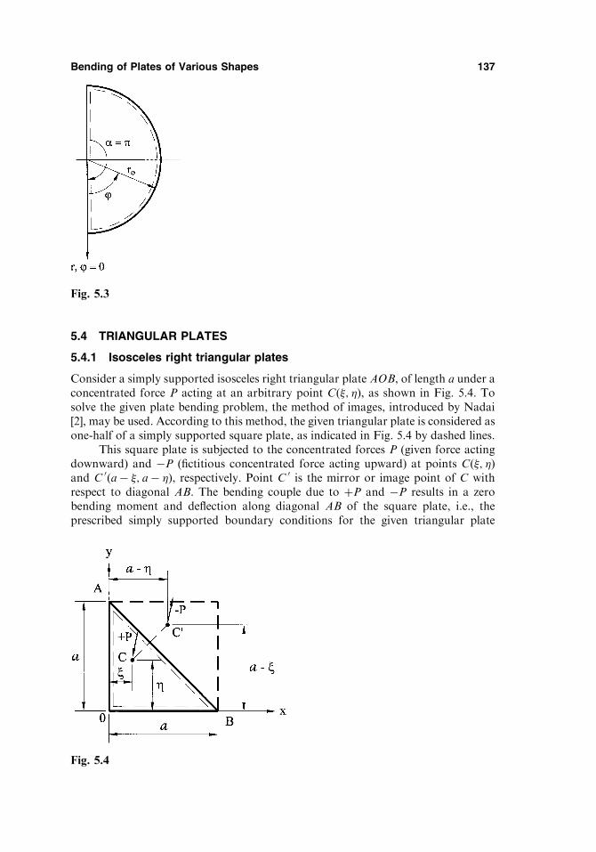
5.4 TRIANGULAR PLATES

5.4.1 Isosceles right triangular plates

Consider a simply supported isosceles right triangular plate AOB, of length a under aconcentrated force P acting at an arbitrary point Cð�; Þ, as shown in Fig. 5.4. Tosolve the given plate bending problem, the method of images, introduced by Nadai[2], may be used. According to this method, the given triangular plate is considered asone-half of a simply supported square plate, as indicated in Fig. 5.4 by dashed lines.

This square plate is subjected to the concentrated forces P (given force actingdownward) and �P (fictitious concentrated force acting upward) at points C �; ð Þand C 0 a� �; a� ð Þ, respectively. Point C 0 is the mirror or image point of C withrespect to diagonal AB. The bending couple due to þP and �P results in a zerobending moment and deflection along diagonal AB of the square plate, i.e., theprescribed simply supported boundary conditions for the given triangular plate

Bending of Plates of Various Shapes 137

Fig. 5.3

Fig. 5.4

� ¼ x� y tan ’ and ¼ 1

cos ’y: ð5:20Þ

Substitution of the expressions (5.20) into Eq. (2.17), transforms the Laplacianoperator from the rectangular to oblique coordinate system, r2

o, as follows:

r2o ¼ 1

cos2 ’

@2

@�2� 2 sin ’

@2

@�@ þ @2

@ 2

!ð5:21Þ

Therefore, the governing differential equation of plate bending, expressed in terms ofthe oblique coordinates, is of the form

D

cos4 ’

@4w

@�4þ 2 1þ 2 sin2 ’

� � @4w

@�2@ 2

(� 4 sin ’

@4w

@�3@ þ @4w

@�@ 3

!þ @

4w

@ 4

)¼ p �; ð Þ:

ð5:22Þor, more concisely,

Dr2or2

ow �; ð Þ ¼ p �; ð Þ: ð5:23ÞThe analytical solution of Eq. (5.22) or (5.23) is complicated by the absence of

orthogonal relationships and by the presence of singularities occurring at the obtusecorners. It can be solved only for a few particular cases. Thus, the analysis of theskew plates mentioned above can be carried out, primarily, by numerical methodsdiscussed in Chapter 6. Some numerical solution procedures and the correspondingexamples are discussed in Szillard [3].

PROBLEMS

5.1 Derive the equation for the bending moments, Mx and My, for a clamped elliptical

plate under a uniformly distributed surface load p0.

5.2 Derive the equations for the shear forces, Qx and Qy, for a clamped elliptical plate

under a uniformly distributed surface load p0.

140 Chapter 5

Fig. 5.6

6

Plate Bending by Approximate andNumerical Methods

6.1 INTRODUCTION

An exact solution in analytical form (i.e., exact solution formula) of plate bendingproblems using classical methods, discussed in Chapters 3, 4, and 5, is limited torelatively simple plate geometry, load configuration, and boundary supports. If theseconditions are more complicated, the classical analysis methods become increasinglytedious or even impossible. In such cases, approximate methods are the onlyapproaches that can be employed for the solution of practically important platebending problems. Nevertheless, the classical solutions remain very valuable becausethey enable one to gain insight into the variation of stresses and strains with basicshape and property changes, and they provide an understanding of the physical platebehavior under an applied loading. In addition, they can be used as a basis forincisively evaluating the results of approximate solutions through quantitative com-parisons and order-of-magnitude bounds.

In this chapter we consider some approximate methods that are widely used forplate and shell bending analysis. By convention, these approximate methods may bedivided into two groups.

6.1.1 Indirect methods

These methods enable us to obtain numerical values of unknown functions by,primarily, direct discretization of the governing differential equation of the corre-sponding boundary value problem. Also they can be defined as methods for solvingproblems on computers. Note that computers have changed, almost revolutionized,numerical methods. These changes of the field as a whole, as well as many individualmethods, are continuing. Here, we introduce such well-known methods as the finitedifference method, the method of boundary collocations, the boundary elementmethod, and the Galerkin method.

143

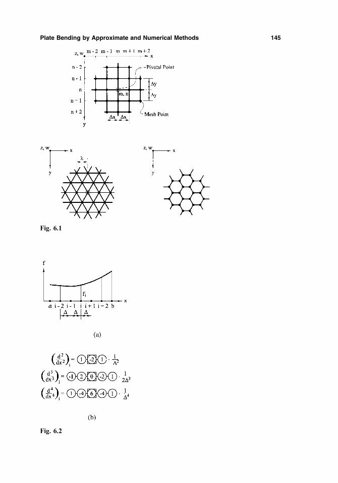
Plate Bending by Approximate and Numerical Methods 145

Fig. 6.1

Fig. 6.2

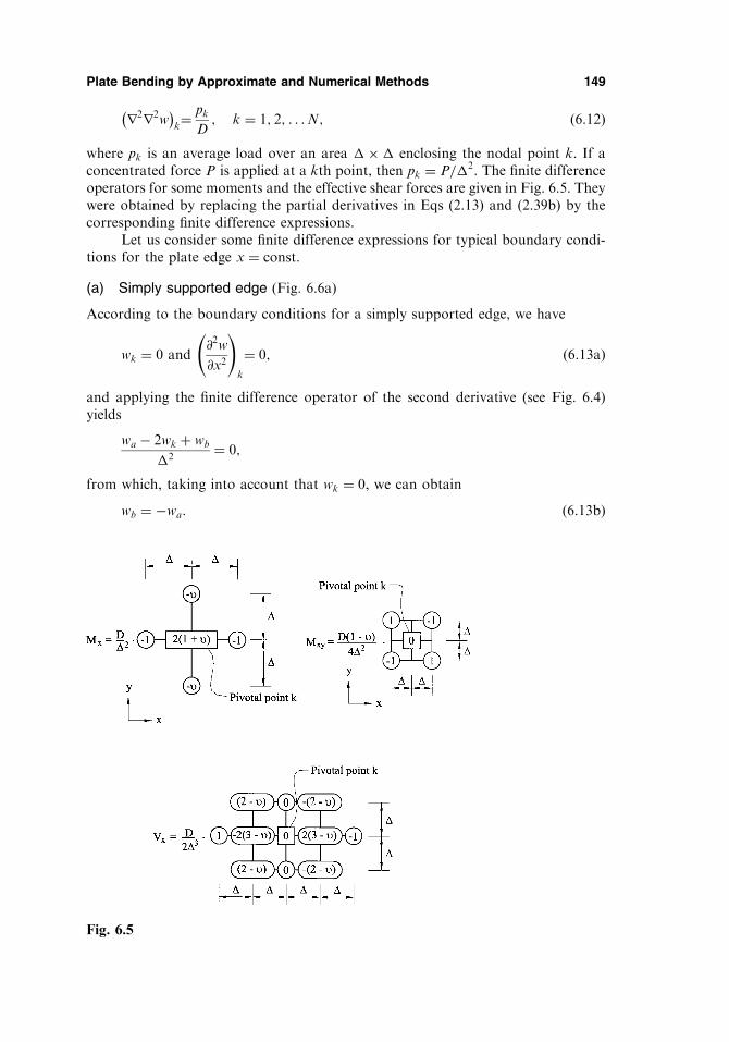
r2r2w� �

k¼ pk

D; k ¼ 1; 2; . . .N; ð6:12Þ

where pk is an average load over an area �� enclosing the nodal point k. If aconcentrated force P is applied at a kth point, then pk ¼ P=�2. The finite differenceoperators for some moments and the effective shear forces are given in Fig. 6.5. Theywere obtained by replacing the partial derivatives in Eqs (2.13) and (2.39b) by thecorresponding finite difference expressions.

Let us consider some finite difference expressions for typical boundary condi-tions for the plate edge x ¼ const:

(a) Simply supported edge (Fig. 6.6a)

According to the boundary conditions for a simply supported edge, we have

wk ¼ 0 and@2w

@x2

!k

¼ 0; ð6:13aÞ

and applying the finite difference operator of the second derivative (see Fig. 6.4)yields

wa � 2wk þ wb

�2¼ 0;

from which, taking into account that wk ¼ 0, we can obtain

wb ¼ �wa: ð6:13bÞ


Fig. 6.5

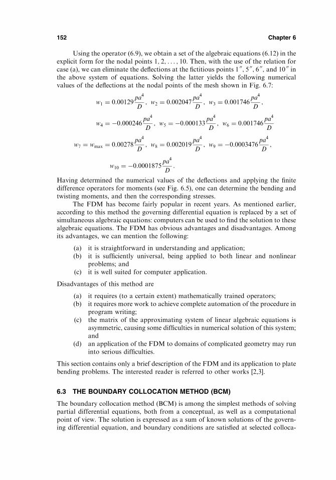
Using the operator (6.9), we obtain a set of the algebraic equations (6.12) in theexplicit form for the nodal points 1; 2; . . . ; 10. Then, with the use of the relation forcase (a), we can eliminate the deflections at the fictitious points 1 00; 5 00; 6 00; and 10 00 inthe above system of equations. Solving the latter yields the following numericalvalues of the deflections at the nodal points of the mesh shown in Fig. 6.7:

w1 ¼ 0:00129pa4

D; w2 ¼ 0:002047

pa4

D; w3 ¼ 0:001746

pa4

D;

w4 ¼ �0:000246pa4

D; w5 ¼ �0:000133

pa4

D; w6 ¼ 0:001746

pa4

D

w7 ¼ wmax ¼ 0:00278pa4

D; w8 ¼ 0:002019

pa4

D; w9 ¼ �0:0003476

pa4

D;

w10 ¼ �0:0001875pa4

D:

Having determined the numerical values of the deflections and applying the finitedifference operators for moments (see Fig. 6.5), one can determine the bending andtwisting moments, and then the corresponding stresses.

The FDM has become fairly popular in recent years. As mentioned earlier,according to this method the governing differential equation is replaced by a set ofsimultaneous algebraic equations: computers can be used to find the solution to thesealgebraic equations. The FDM has obvious advantages and disadvantages. Amongits advantages, we can mention the following:

(a) it is straightforward in understanding and application;(b) it is sufficiently universal, being applied to both linear and nonlinear

problems; and(c) it is well suited for computer application.

Disadvantages of this method are

(a) it requires (to a certain extent) mathematically trained operators;(b) it requires more work to achieve complete automation of the procedure in

program writing;(c) the matrix of the approximating system of linear algebraic equations is

asymmetric, causing some difficulties in numerical solution of this system;and

(d) an application of the FDM to domains of complicated geometry may runinto serious difficulties.

This section contains only a brief description of the FDM and its application to platebending problems. The interested reader is referred to other works [2,3].

6.3 THE BOUNDARY COLLOCATION METHOD (BCM)

The boundary collocation method (BCM) is among the simplest methods of solvingpartial differential equations, both from a conceptual, as well as a computationalpoint of view. The solution is expressed as a sum of known solutions of the govern-ing differential equation, and boundary conditions are satisfied at selected colloca-

152 Chapter 6

In the expressions (6.18) r and ’ are polar coordinates of points of interest with theorigin located somewhere within the plate. Each term in the left set of braces timeseach term in the right set of braces in (6.18) represents a solution form and satisfiesthe homogeneous differential equation (2.24). Other forms of the basic functions arediscussed in [5, 8].

In dealing with solid plates with a centrally placed origin, all singular terms inthe expressions (6.18) and (6.19) (lnr; rlnr, and r to any negative power) are omitted.As it follows from the above, w x; yð Þ in the form of (6.17) satisfies Eq. (2.24) exactly.Thus, only the boundary conditions need to be satisfied. Substituting the expressions(6.17) into Eqs. (6.16) and assuming that the boundary conditions will be satisfied atsome discrete points (xi; yi; i ¼ 1; 2; . . . ;M), called collocation points, along bound-ary �, leads to a system of 2M linear algebraic equations for N unknown constantsaj. This system can be written in the following form:

A½ � af g ¼ bf g; ð6:20Þwhere A½ � ¼ ½Aij;AiþM;j�T and fbg ¼ ½bi; biþM �T are the partitioned matrices. Thecoefficients of these matrices are of the form

Aij ¼ l1½�jðxi; yÞ�;AiþM;j ¼ l2½�jðxi; yiÞ�;bi ¼ f1ðxi; yiÞ � l1½wpðxi; yiÞ�; biþM ¼ f2ðxi; yiÞ � l2½wpðxi; yiÞ�

fag is the column matrix of unknown coefficients aj. In order to obtain a squarematrix [A], the number of terms in the expansion (6.17) would have to be twice thenumber of collocation points, that is, N ¼ 2M. Such a variant of the BCM is calledthe straightforward boundary collocation method.

As an alternative to insuring that the matrix A½ � is square by a proper choice ofterms and boundary conditions, one can go to the process known as the over-determined boundary collocation method. In the latter approach, more collocationpoints are chosen than are necessary, i.e., 2M > N, and the system (6.20) containsmore equations than unknowns. This overdetermined system can be solved by theleast squares method [2]. This numerical procedure is quite simple. Let fa g be a trialsolution of Eq. (6.20). fa g does not exactly satisfy Eq. (6.20) but leads to someresidual error feg, so that

½A�fa g � fbg ¼ feg ð6:21ÞIt can be shown the condition for selecting the solution fa g to minimize the

error ei is equivalent to the following matrix equation [5]

A½ �T � A½ � � a � � ¼ A½ �T � bf g ð6:22Þ

The matrix A½ �T � A½ � is square and positive definite. The system of linear algebraicequations (6.22) is called the normal system. The solution steps are the same as for asquare matrix.

In conclusion, notice that the BCM has some advantages and disadvantages.Among the advantages one notes the following:

1. it is easy to understand and program the approach;2. it is easily applied to arbitrary shapes and boundary conditions, and the

solution appears in a closed form for the whole region.

154 Chapter 6

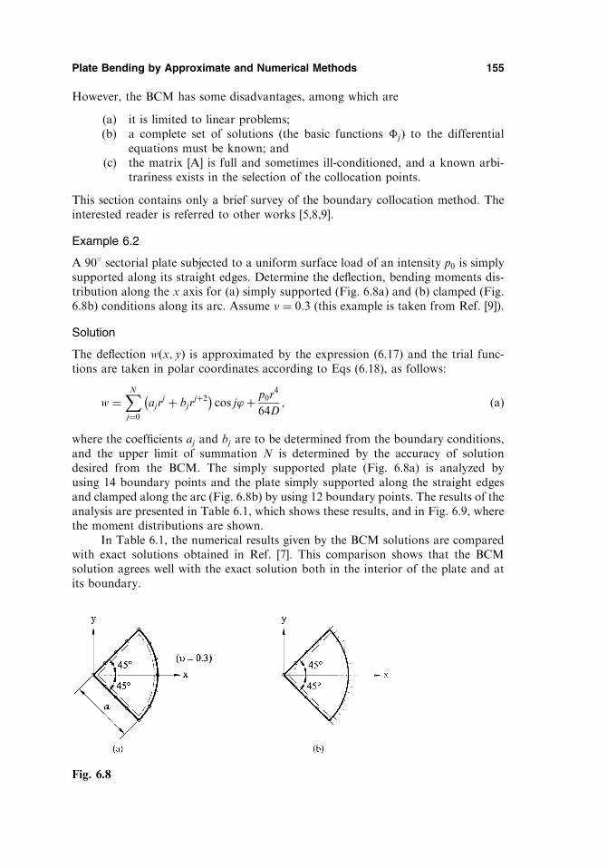
However, the BCM has some disadvantages, among which are

(a) it is limited to linear problems;(b) a complete set of solutions (the basic functions �j) to the differential

equations must be known; and(c) the matrix A½ � is full and sometimes ill-conditioned, and a known arbi-

trariness exists in the selection of the collocation points.

This section contains only a brief survey of the boundary collocation method. Theinterested reader is referred to other works [5,8,9].

Example 6.2

A 90 sectorial plate subjected to a uniform surface load of an intensity p0 is simplysupported along its straight edges. Determine the deflection, bending moments dis-tribution along the x axis for (a) simply supported (Fig. 6.8a) and (b) clamped (Fig.6.8b) conditions along its arc. Assume � ¼ 0:3 (this example is taken from Ref. [9]).

Solution

The deflection wðx; yÞ is approximated by the expression (6.17) and the trial func-tions are taken in polar coordinates according to Eqs (6.18), as follows:

w ¼XNj¼0

ajrj þ bjr

jþ2� �

cos j’þ p0r4

64D; ðaÞ

where the coefficients aj and bj are to be determined from the boundary conditions,and the upper limit of summation N is determined by the accuracy of solutiondesired from the BCM. The simply supported plate (Fig. 6.8a) is analyzed byusing 14 boundary points and the plate simply supported along the straight edgesand clamped along the arc (Fig. 6.8b) by using 12 boundary points. The results of theanalysis are presented in Table 6.1, which shows these results, and in Fig. 6.9, wherethe moment distributions are shown.

In Table 6.1, the numerical results given by the BCM solutions are comparedwith exact solutions obtained in Ref. [7]. This comparison shows that the BCMsolution agrees well with the exact solution both in the interior of the plate and atits boundary.


Fig. 6.8

6.4 THE BOUNDARY ELEMENT METHOD

The boundary element method (BEM) is now used extensively for the analysis oftwo-dimensional (2D) and three-dimensional (3D) elastic, homogeneous, and iso-tropic bodies. It offers important advantages over domain-type methods, such as thefinite element method and the finite difference method, since only the discretizationof the boundary is needed. The BEM is well suited for treating complicated bound-aries, for discontinuous internal actions, mixed boundary conditions, etc. In parti-cular, the BEM has been applied successfully for the solutions of plate bendingproblems, demonstrating its advantages [10–14].

The BEM reduces a given boundary value problem for a plate, in the form ofpartial differential equations to the integral equations over the boundary of the plate.Then, the BEM proceeds to obtain an approximate solution by solving these integralequations. To make such a reduction possible, it is necessary, first, to express thesolution as the sum of a particular integral corresponding to a given loading appliedto the plate and of a complementary solution. That solution satisfies the homoge-neous partial differential equation corresponding to the load-free plate, subject tocertain boundary conditions.

156 Chapter 6

Table 6.1

Simple arc support Clamped arc support

w Mx My w Mx

x=a Exact BCM Exact BCM Exact BCM Exact BCM Exact BCM

0 0 0 — �271 — 271 0 0 — �199

0.25 92 93 36 38 319 322 63 64 68 70

0.50 225 226 353 354 352 353 132 132 272 273

0.75 203 203 381 381 286 287 82 81 113 116

1.00 0 0 0 0 88 88 0 1 �488 �486

Multi. 10�5p0a4=D 10�4p0a

2 10�4p0a2 10�5p0a

4=D 10�4p0a2

Fig. 6.9

Several different boundary element approaches have already been proposed forthe construction of the complementary solution. They are frequently referred to asdirect and indirect BEM formulations [12,13]. In the indirect BEM formulation, thecomplementary function is represented by an integral in terms of some arbitraryfunctions, called source functions, over the boundary of a domain of the plate. Thesesource functions may be visualized, for example, as fictitious force and momentdistributions acting on the boundary of the given plate embedded in an infiniteelastic plate (the term ‘‘fictitious’’ is used here because these loads are not resultingin transverse loads assigned for the plate). Finding these source functions, one candetermine the deflections, bending and twisting moments anywhere within the plateor on its boundary.

In the direct formulation, the partial differential equation of the plate bendingproblem for the complementary function is transformed by the use of the reciprocalwork identity to an integral equation in terms of boundary values of the deflectionsand the stress resultants. Both BEM formulations have certain advantages and dis-advantages that are discussed in detail in Refs [12,13]. It has been established nowthat these two formulations have the same origin and theoretical basis. We discussbelow both approaches, as applied to plate bending problems.

6.4.1 Indirect BEM for plates

The presentation of the indirect BEM below follows the approach of Ventsel [14].Assume that a given plate, originally occupying a 2D domain � with a smoothboundary �, is to be extended infinitely. Then, apply to an infinite plate theabove-mentioned fictitious loads in the form of transverse loads qð�; Þ and momentsmnð�; Þ distributed continuously over �, where ð�; Þ is some point on � (called thesource point). The moments mn act in the direction of the outward normal n to � atthe source point (Fig. 6.10).

In order to determine the deflection surface of the infinite plate caused by theabove-mentioned fictitious loads, find the so-called singular solutions of the bihar-monic equation (2.24). In our case, these singular solutions correspond to the deflec-tion of point ðx; yÞ of the infinite plate (called the observation point) caused by a unitnormal concentrated force, and by a unit concentrated moment; both are applied at


Fig. 6.10

required to find the slopes, moments, and shear forces in the plate due to thesefictitious loads applied along �.

Assume that the boundary conditions on � are nonhomogeneous, as follows:

w ¼ w �; #n ;¼ # n

�

(Problem 1);

w ¼ w �; Mn ¼ M

n

�

(Problem 2),

Mn ¼ M n

�; Vn ¼ V

n

�

(Problem 3),

ð6:27Þ

where #n;Mn; and Vn are the slope, bending moment, and the effective shear forceon the boundary with the outer normal n;# n;M

n ; and V

n are given boundaryfunctions specified on �. The boundary quantities #n;Mn; and Vn at a regularpoint on � are expressed in terms of the deflection w by the relations (2.45)–(2.48)and Eq. (2.13). We obtain the following:

#n ¼@w

@n;

Mn ¼ �D@2w

@n2þ � @

2w

@t2

!;

Vn ¼ �D@3w

@n3þ 2� �ð Þ @

3w

@n@t2

" #;

ð6:28Þ

where @=@n and @=@t denote differentiation along the outward normal and tangentialdirections, respectively.

The expression (6.25) satisfies the governing equation (2.24) exactly and doesnot satisfy the prescribed boundary conditions (6.27) for arbitrary chosen fictitiousloads q and mn. Inserting wðx; yÞ in the form of Eq. (6.25) into the boundary con-ditions (6.27) and letting a point ðx;yÞ from inside the domain approach the bound-ary, we obtain the integral representation of the deflection, slope, normal bendingmoment, and the effective shear force on � due to the given and fictitious loads. In sodoing, it is necessary to take the limit as x; y approaches �, and to examine thelimiting values of the above-mentioned integral representations. It can be shown thatthe deflections and slopes remain continuous, whereas the normal bending momentsand effective shear forces undergo a finite jump for a passage through the boundary�. Equating the limiting values of w x; yð Þ; #n x; yð Þ;Mn x; yð Þ; and Vn x; yð Þ on � to theprescribed boundary functions according to Eqs (6.28), we finally obtain the bound-ary integral equations for the unknown fictitious loads q �; ð Þ and mn �; ð Þ. Theseequations can be represented in the general form for solving Problems 1, 2, and 3, asfollows:ð

�

qð�; ÞGqðx; y; �; Þ þmnð�; ÞGmðx; y; �; Þ� �

dsþ wpðx; yÞ ¼ w ðx; yÞ;

ð6:29aÞð�

qð�; Þ @2Gqðx; y; �; Þ

@nþmnð�; Þ

@Gmðx; y; �; Þ@n

" #dsþ @wpðx; yÞ

@n¼ # nðx; yÞ;

ð6:29bÞ


ð�

qð�; nÞ @2Gqðx; y; �; Þ@n2

þ � @2Gqðx; y; �; Þ

@t2

!" #dsþmnðx; yÞ

2

þð�

mnð�; Þ@2Gmðx; y; �; Þ

@n2þ � @

2Gmðx; y; �; Þ@t2

!" #ds

þ @2

@n2þ � @

2

@t2

!wpðx; yÞ ¼ M

n ðx; yÞ; ð6:29cÞ

1

2qðx; yÞ þ

ð�

qð�; Þ @3Gqðx; y; �; Þ

@n3þ ð2� �Þ @

3Gqðx; y; �; Þ@n@t2

" #ds

þð�

mnð�; Þ@3Gmðx; y; �; Þ

@n3þ ð2� �Þ @

3Gmðx; y; �; Þ@n@t2

" #ds

þ @3

@n3þ ð2� �Þ @3

@n@t2

" #wpðx; yÞ ¼ V

n ðx; yÞ: ð6:29dÞ

It can be shown [14] that the kernels of the integrals in Eqs (6.29a)–(6.29c), as wellas the first integral in Eq. (6.29d), are bounded when a point ðx; yÞ from thedomain � approaches �; ð Þ on �: Therefore, the integrals of these equations canbe evaluated by using a standard numerical technique developed for the numericalimplementation of regular integrals. The kernel of the second integral in Eq.(6.29d) behaves like r�2 when a point x; yð Þ ! �; ð Þ on the boundary. This integraldoes not exist neither as an improper nor singular integral and special care must betaken for representation and evaluation of such a type of integral. There are anumber of efficient techniques for dealing with this strongly singular integral [14–16]. The first approach is to cancel out explicitly this higher-order singularity inadvance, before limiting transition to the boundary (for example, by using integra-tion by parts for the expression of the effective shear force when a point x; yð Þ isnot on �). The second possibility is to assign a certain sense to this stronglysingular integral. This is possible because it appears in the expression for theeffective shear force which is finite on the boundary. Hadamard [17] defined thisintegral in the finite part integration sense and it is referred to as a hypersingularintegral. Hypersingular integrals can be evaluated analytically, using either someregularization technique [14–17, etc.], or numerically, by special quadrature for-mulas that avoid any explicit performing of limiting processes [14,18,19].

Solving the boundary integral equations, we obtain the source functions q �; ð Þand mn �; ð Þ distributed over �. Once the fictitious loads q and mn distributed overthe boundary have been established from the numerical solution of the boundaryintegral equations, the values of the deflection and stress resultants anywhere withinthe plate and on its boundary can be calculated by using Eqs (6.25) and (2.13).

6.4.2 Direct BEM

Unlike the indirect BEM, the direct BEM is formulated in terms of the naturalvariables, interpretable as deflection, slope, bending moment, and effective shearforce assigned along the plate boundary �.

160 Chapter 6

differentiating Eq. (6.32) in a fixed direction v, we obtain, through a limiting process,the following integral representation of the slopes:

c#vð�; Þ ¼ð�

Vn wh i @Gq

@v�Mn wh i @

2Gq

@n@v� Vn

@Gq

@v

� �wþMn

@Gq

@v

� �#n

" #dsðx; yÞ

þð ð�

pðx; yÞ @Gq

@vd�ðx; yÞ

ð6:34Þwhere c for a smooth boundary at point (x; yÞ is given by (6.32), #v ¼ @w=@v.

The expressions (6.32) and (6.34) can be used to give the boundary integralequations of the direct BEM. Indeed, placing in the above equations the point ð�; Þon the boundary �, replacing two out of four boundary quantities, w; #n;Mn; andVn, by prescribed boundary functions according to Eqs. (6.27), and noting that theboundary functions on the left sides are the same boundary functions as on the rightsides, we can formulate two coupled boundary integral equations for the two remain-ing boundary quantities.

Comparing the indirect and direct BEM formulations, it is easy to discoverthat the variables ðx; yÞ and ð�; Þ change places in the resulting boundary integralequations (6.29) and (6.32), (6.34).

6.4.3 Numerical treatment of BEM

An analytical solution of the boundary integral equations of either direct or indirectBEM formulation is possible in the exceptional cases of a simple plate geometry,load, and boundary conditions. However, these equations can be solved numericallyby employing the standard boundary element technique developed, for example, inRefs [11–13].

Let us describe briefly a possible numerical procedure for solving these bound-ary integral equations. The boundary of a given domain is divided into N smoothboundary elements (BEs), ��k k ¼ 1; 2; . . .Nð Þ. The geometry of ��k is approxi-mated by a straight line or a parabolic arc. Unknown source functions (either‘‘fictitious’’ loads in the indirect BEM or natural variables in the direct BEM) areassumed to be uniformly or linearly varying along ��k (of course, a higher order ofapproximation of these functions can be also assigned). The nodes of the unknownsource functions and the given boundary functions are assigned either at the centerof ��k or at the interfaces between two adjacent boundary elements. The integralsare evaluated analytically or numerically using standard Gaussian quadrature [21].In the case where the boundary integrals involve the previously mentioned strongsingularities (when a point x; yð Þ 2 � ! ð�; Þ 2 �), it is necessary to consider aneighborhood of such points separately and employ the special regularization for-mulas [14–19] for evaluating these singular integrals. Such an approximation of theboundary integral equations yields a system of algebraic equations with respect tonodal values of the unknown source functions. Once these unknowns have beenestablished, the values of the deflections and stress resultants at any point eitherinside the plate domain or on its boundary can be evaluated from the discretizedform of Eqs (6.25), (6.32), and (2.13).

162 Chapter 6

Solution

This problem was analyzed by Ventsel [14]. He applied the indirect BEM to theanalysis of the plate. The plate boundary was divided into 28 boundary elements(BEs), giving a total of 28 nodes. The boundary conditions were satisfied at thesenodal points. Unknown edge forces, q, and the normal edge moments, mn, wereassumed to be constant over BEs. The two boundary integral equations (Eqs(6.29a) and (6.29b)) were approximated by 56 algebraic equations for the 56 nodalloads, q kð Þ and m kð Þ

n k ¼ 1; 2; . . . ; 28ð Þ. Some results of the numerical analysis areshown in Fig. 6.12a, b in the form of the deflection and bending moment distribu-tions along section AB and the boundary. The deflection and bending momentsordinates are given in Fig. 6.12 to within the following constant multipliers: p=Dfor the w and P for the function M.

In conclusion, it should be noted that the BEM is very powerful and efficient asapplied to various linear plate bending problems. The method has the followingadvantages:

1. It can be easily adapted to any complicated geometry of the domaininvolved and to arbitrary boundary conditions, like the finite elementmethod. However, unlike the FEM, an application of the BEM to bound-ary value problems enables us to reduce the dimensionality of the pro-blem. The latter results in a smaller, than the FEM, system of equationsand considerable reductions in the data required to run a problem.

2. The BEM is easily programmed for arbitrary plate configurations, loads,and boundary conditions.

3. The numerical accuracy of the BEM is generally greater than that of theFEM and other numerical methods. The numerical discretization of themethod leads to a stable system of linear algebraic equations. The error ofan approximate solution introduced by the BEM can be estimated aposteriori when the problem under consideration has been solved [14].

4. The method has been adapted well for the solution of the so-called sin-gular problems, such as plates with crack-like defects, plates having holes,corners, etc.

However, this method has some disadvantages:

1. It can be successfully applied primarily to linear problems.2. The method requires that a fundamental solution of a governing differ-

ential equation or Green’s function be represented in the explicit analy-

164 Chapter 6

Table 6.2

Displacement ðpa4=100DÞBoundary element method

Point Indirect Direct Finite element method Finite difference method

A 0.2188 0.2188 0.2185 0.2174

B 0.3107 0.3141 0.3156 0.3006

C 0.1558 0.1565 — 0.1541

Substituting for wN from Eq. (6.36), one obtains

ð ðA

LXNi¼1

ifiðx; yÞ !

� p

" #fjðx; yÞdxdy ¼ 0; j ¼ 1; 2; . . . ;N:

Introducing the residual error function EðwNÞ, as follows,

EðwNÞ ¼ LXNi¼1

ifiðx; yÞ !

� p; ð6:38Þ

we can rewrite the above Galerkin equation in the formð ðA

E i; fiðx; yÞ; pð Þfjðx; yÞdxdy ¼ 0; i; j ¼ 1; 2; . . . ;N: ð6:39Þ

The above requirement can be used as a condition for determining the coefficients i.Replacing the integral in Eq. (6.39) by the sum of integrals, we obtain the followingsystem of linear algebraic equations:

a111 þ a122 þ ::::: þ a1NN ¼ b1

. . . . . . . . . . . . . . . . . . . . . . . . . . . . . . . . .

aN11 þ aN22 þ :::::þ aNNN ¼ bN;

ð6:40aÞ

where

aij ¼ð ð

A

L fið Þ � fjdxdy; bi ¼ð ð

A

p � fjdxdy i; j ¼ 1; 2; . . . ;N: ð6:40bÞ

Solving Eqs (6.40a), we can determine the unknown coefficients i which, in con-junction with Eq. (6.36), gives the N-parameter Galerkin approximation of Eq.(6.35). Notice that if N ! 1, the Galerkin solution approaches the exact solutionif the system of functions f1; f2; . . . is complete and linearly independent [6].

Galerkin equations (6.37) had been derived above from the special mathema-tical condition of orthogonality of two functions, Eq. (a). However, the Galerkinmethod can be derived from the general variational principle of virtual work, intro-duced in Sec. 2.6.2.

As shown in Sec. 2.4, the governing equation of plate bending problems, Eq.(2.24), represents the condition of static equilibrium of an infinitesimal plate element.Then, the operator ½LðwNÞ � p� can be interpreted as an intensity of some unbalancedtotal loading that occurs over the area of integration A (area of the plate) when thedeflection function is sought in the form of Eq. (6.36). Retaining a finite number of Nterms in the expansion (6.36) implies that an actual continual system is replaced by asystem withN degrees of freedom (i.e., a discrete system). In turn, the constant coeffi-cients i (i ¼ 1; 2; . . . ;NÞ can be treated as some generalized displacements, each ofwhich corresponds to a deflected state of the plate defined by a function fiðx; yÞ.

According to the principle of virtual work, any discrete system is in equilibriumif work done by all the elementary forces, i.e., LðwNÞ � p½ �dxdy, acting through someadmissible for this system displacements, i.e., �ifiðx; yÞ, is equal to zero:


w ¼ 1 x2 � a2� �2

a4; ðeÞ

Mx ¼ �D@2w

@x2

y¼0

¼ �4D1 3x2 � a2� �

a4: ðfÞ

The maximum bending moment occurs at midpoints of the sides x ¼ �a; y ¼ 0, andMmax is given by

Mmax ¼ �8D1a6 ¼ �0:171pa2:

The exact solution of Mmax found by Galerkin is �0:204pa2 [22]. The error is about16%, which is higher than for the deflection. Taking more terms in the expression(b), we approach the above exact value of the bending moment.

It should be noted that the Galerkin method is more general that the Ritzmethod discussed in Sec. 6.6, because no quadratic functional or virtual work prin-ciple is necessary. If the governing equations are derivable from a variational prin-ciple, then the Galerkin method reduces to the Ritz method and leads to an identicalset of linear algebraic equations produced by the Ritz method. Sometimes, theGalerkin method may be preferable if it is more convenient to work with the govern-ing differential equations rather than with the energy functional. Moreover, there areproblems for which no satisfactory variational principle has been formulated, but forwhich a set of governing differential equations is available. This suggests that theGalerkin method is even broader in application than the Ritz method.

6.6 THE RITZ METHOD

We are now coming to the presentation of the direct methods. We begin with a studyof the Ritz method. The Ritz method belongs among the so-called variational meth-ods that are commonly used as approximate methods for a solution of variousboundary value problems of mechanics. These methods are based on variationalprinciples of mechanics discussed in Sec. 2.6.

The energy method developed by Ritz [23] applies the principle of minimumpotential energy (2.64). According to the Ritz method, the deflection surface of theplate is approximated by series of the form

w x; yð Þ ¼X1i¼1

Cifi x; yð Þ; ð6:42Þ

where fi x; yð Þ are some coordinate functions that satisfy individually, at least, thekinematic boundary conditions (i.e., conditions imposed on the deflections and theirfirst derivatives) and Ci are unknown constants to be determined from the minimumpotential energy principle.

Introducing the expression for w x; yð Þ in the form of (6.42) into Eq. (2.60) forthe total potential energy of a plate, we obtain the following after integrating thetotal potential energy � as a function of the unknown coefficients Ci:

� ¼ � C1;C2; . . .ð Þ: ð6:43Þ


The coordinate functions fi x; yð Þ must satisfy the boundary conditions (a) onlyand they must not satisfy the natural boundary conditions for the free edge x ¼ aand the second boundary condition (My ¼ 0) for simply supported edges y ¼ 0and y ¼ b. Let us take an approximate solution of the following form (the firstapproximation):

w x; yð Þ ¼ C1

x

a

� �2sin�y

b; ðbÞ

where C1 is an unknown coefficient. It can be easily shown that w x; yð Þ in the form ofEq. (b) satisfies exactly the boundary conditions (a) and does not violate the condi-tions of w 6¼ 0 and @w=@x 6¼ 0 along the free edge, and @w=@y 6¼ 0 along the simplysupported edges. Let us introduce new dimensionless coordinates � and , as follows:

x ¼ a� and y ¼ b : ðcÞThus, we can rewrite the expression for the total potential energy (Eq. (2.60)) in newcoordinates as

� ¼ Db

2a3

ð10

ð10

@2w

@�2

!þ a

b

� �2 @2w

@ 2

!" #28<:

�2 1� �ð Þ a

b

� �2 @2w

@�2@2w

@ 2� @2w

@�@

!224

359=;d�d � ab

ð10

ð10

p � wd�d ;

ðdÞ

and the expression for the deflection surface is

w ¼ C1�2 sin� : ðeÞ

Upon substituting the expression (e) for the deflection into Eq. (d), evaluating theintegrals and taking the derivative @�=@C1 ¼ 0, we can determine coefficient C1. Wehave C1 ¼ a4p=D

� �2=�ð Þ, where � is given by

� ¼ 3� 2þ �4

10

a

b

� �4þ 4

3�2 ð1� �Þ a

b

� �2� 2

3��2

a

b

� �2� �:

"ðfÞ


Fig. 6.14

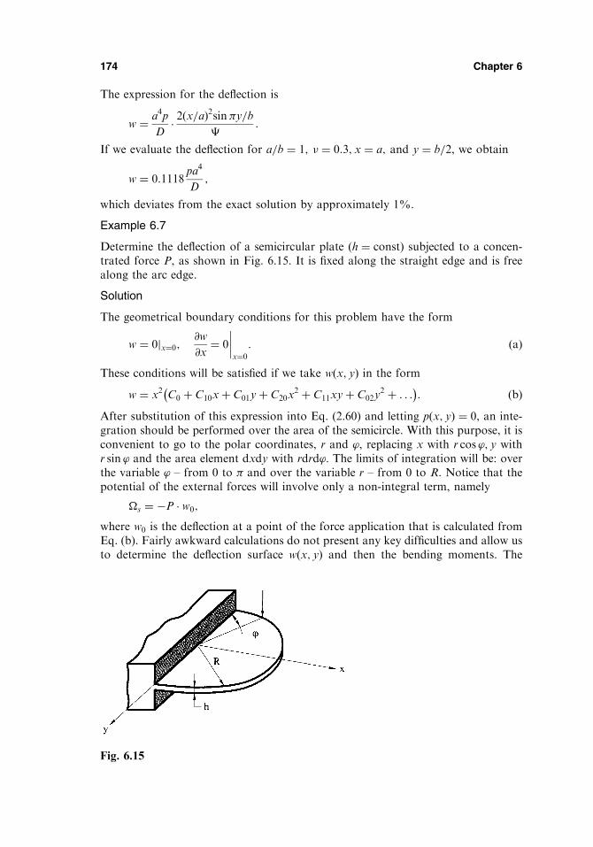
The expression for the deflection is

w ¼ a4p

D� 2 x=að Þ2sin�y=b

�:

If we evaluate the deflection for a=b ¼ 1; � ¼ 0:3; x ¼ a; and y ¼ b=2, we obtain

w ¼ 0:1118pa4

D;

which deviates from the exact solution by approximately 1%.

Example 6.7

Determine the deflection of a semicircular plate (h ¼ constÞ subjected to a concen-trated force P, as shown in Fig. 6.15. It is fixed along the straight edge and is freealong the arc edge.

Solution

The geometrical boundary conditions for this problem have the form

w ¼ 0jx¼0;@w

@x¼ 0

x¼0

: ðaÞ

These conditions will be satisfied if we take w x; yð Þ in the form

w ¼ x2 C0 þ C10xþ C01yþ C20x2 þ C11xyþ C02y

2 þ . . .� �

: ðbÞAfter substitution of this expression into Eq. (2.60) and letting p x; yð Þ ¼ 0, an inte-gration should be performed over the area of the semicircle. With this purpose, it isconvenient to go to the polar coordinates, r and ’, replacing x with r cos ’; y withr sin ’ and the area element dxdy with rdrd’. The limits of integration will be: overthe variable ’ – from 0 to � and over the variable r – from 0 to R. Notice that thepotential of the external forces will involve only a non-integral term, namely

�s ¼ �P � w0;

where w0 is the deflection at a point of the force application that is calculated fromEq. (b). Fairly awkward calculations do not present any key difficulties and allow usto determine the deflection surface w x; yð Þ and then the bending moments. The

174 Chapter 6

Fig. 6.15

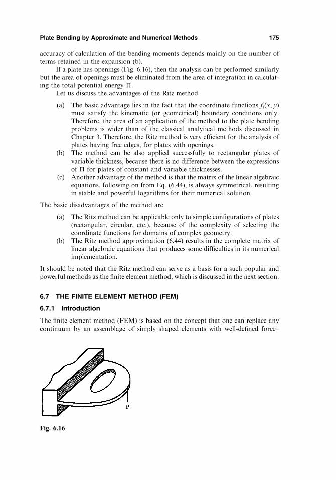
accuracy of calculation of the bending moments depends mainly on the number ofterms retained in the expansion (b).

If a plate has openings (Fig. 6.16), then the analysis can be performed similarlybut the area of openings must be eliminated from the area of integration in calculat-ing the total potential energy �.

Let us discuss the advantages of the Ritz method.

(a) The basic advantage lies in the fact that the coordinate functions fi x; yð Þmust satisfy the kinematic (or geometrical) boundary conditions only.Therefore, the area of an application of the method to the plate bendingproblems is wider than of the classical analytical methods discussed inChapter 3. Therefore, the Ritz method is very efficient for the analysis ofplates having free edges, for plates with openings.

(b) The method can be also applied successfully to rectangular plates ofvariable thickness, because there is no difference between the expressionsof � for plates of constant and variable thicknesses.

(c) Another advantage of the method is that the matrix of the linear algebraicequations, following on from Eq. (6.44), is always symmetrical, resultingin stable and powerful logarithms for their numerical solution.

The basic disadvantages of the method are

(a) The Ritz method can be applicable only to simple configurations of plates(rectangular, circular, etc.), because of the complexity of selecting thecoordinate functions for domains of complex geometry.

(b) The Ritz method approximation (6.44) results in the complete matrix oflinear algebraic equations that produces some difficulties in its numericalimplementation.

It should be noted that the Ritz method can serve as a basis for a such popular andpowerful methods as the finite element method, which is discussed in the next section.

6.7 THE FINITE ELEMENT METHOD (FEM)

6.7.1 Introduction

The finite element method (FEM) is based on the concept that one can replace anycontinuum by an assemblage of simply shaped elements with well-defined force–


Fig. 6.16

displacement and material relationships. While one may not be able to derive aclosed-form solution for the continuum, one can derive an approximate solutionfor the element assemblage that replaced it.

According to the FEM, a plate is discretized into a finite number of elements(usually, triangular or rectangular in shape), called finite elements and connected attheir nodes and along interelement boundaries. Unknown functions (deflections,slopes, internal forces, and moments) are assigned in the form of undeterminedparameters at those nodes. The equilibrium and compatibility conditions must besatisfied at each node and along the boundaries between finite elements. To deter-mine the above-mentioned unknown functions at nodal points, one of the variationalprinciples, introduced in Sec. 2.6, is applied. As a result, a system of algebraicequations is obtained. Its solution determines the state of stress and strain in agiven plate.

There are a number of finite element methods. In this section we discussonly the commonly used finite element displacement approach wherein the gov-erning set of algebraic equations is expressed in terms of unknown nodal displa-cements.

The FEM can be treated as some modification of the Ritz method. A differencebetween the classical Ritz approach and the FEM is in the technique of representa-tion of displacements. In the Ritz method, the displacements are assigned in theentire domain occupied by the plate. A governing system of algebraic equationsfor this approach will have a completed, not banded structure. Since in the FEMthe displacements are assigned element by element, the matrix of the system ofalgebraic equations is obtained as partially completed, and usually it has a bandedstructure. This is a profound advantage of the FEM compared with other numericalmethods introduced in the preceding sections of this chapter.

The FEM has gained considerable attention and prominence after the publica-tion of the classic paper by Turner et al. [26] that showed how one can use anassemblage of simple elements as a basis for computerized structural analysis.Courant [27], and later Argyris et al. [28] represent the initial attempts to providethe theoretical investigations of this method. Gallagher [29], Hughes [30],Zienkiewicz [31], and other investigators developed the general procedure of theFEM technique for plate and shell stress analysis.

For every finite plate (or shell) element there is a relationship between thegeneralized displacements at the nodal points and the corresponding forces andmoments at the nodes. This relationship may be presented in the form of a matrixcalled a stiffness matrix. In this section, we discuss the stiffness matrices for rectan-gular and triangular plate elements. Then, we present the general procedure of theFEM for plate bending analysis. The derivations, given below, are based on theclassical (Kirchhoff’s) plate bending theory introduced in Chapter 2.

6.7.2 The rectangular plate element

Consider a flat rectangular plate which is subdivided into rectangular finite elementswith dimensions c and d, as shown in Fig. 6.17. The properties belonging to such afinite element (abbreviated further as FE) is designated e. The geometrical positionof a rectangular FE is determined by the four nodal (corner) points i; j; k; and l, andthe straight line boundaries. At each node q ðq ¼ i; j; k; lÞ we consider the possible

176 Chapter 6

B½ �i ¼ � @2 L½ �i@x2

;� @2 L½ �i@y2

;�2@2 L½ �i@x@y

" #T

;

B½ �j ¼ � @2 L½ �j@x2

;� @2 L½ �j@y2

;�2@2 L½ �j@x@y

" #T

; etc.

Now. let us introduce the stress resultants and stress couples relationships (see Eqs(2.13)) in the matrix form:

fMge ¼Mx

My

Mxy

8>><>>:

9>>=>>; ¼ D

1 � 0

� 1 0

0 0 ð1� �Þ=2

2664

3775

�x

�y

2�xy

8>><>>:

9>>=>>;; ð6:57aÞ

or symbolically as follows:

Mf ge¼ D½ � �f ge; ð6:57bÞwhere D½ � is the elasticity matrix. The stress–strain relationship, from Eqs (2.10), canbe written in the matrix form as follows:

�f ge¼ z D ½ � �f ge; ð6:58Þwhere the matrix D ½ � is given by

D ½ � ¼ 12

h3D½ �: ð6:59Þ

To continue the development, it is necessary to define the set of discrete nodal forcescorresponding to the prescribed nodal degrees, as shown in Fig. 6.17:

Rf ge¼ Ri;Rj;Rk;Rl

� �T; ð6:60aÞ

where

Rq

� � ¼ Pq;mxq;myq

� �T; q ¼ i; j; k; l: ð6:60bÞ

We now employ the principle of minimum potential energy, introduced in Sec.2.6.2, to derive the element stiffness matrix, k½ �e and the element nodal force matrixRf ge. Toward this end, we write the strain energy in the element as (see Eq. (2.61))

Ue ¼1

2

ð ðAe

�½ �Te Mf gedAe: ð6:61Þ

Substituting for �½ �Te from Eq. (6.56) and for Mf ge from Eq. (6.57b) into the above,we obtain

Ue ¼1

2

ð ðAe

�f gTe B½ �T D½ � B½ � �f gedAe ¼ �f gTe1

2

ð ðAe

B½ �T D½ � B½ �dAe

* +�f ge

or

180 Chapter 6

The results of calculations are given in Table 6.4 (taken from Ref. [32]), where thesenumerical results for varied numbers of the FEs are compared with those obtainedfrom Ref. [7]. As seen from Table 6.4, a discrepancy of the corresponding numericaldata is small even for a sufficiently large mesh of the plate discretization. A reductionof mesh dimensions (an increase in the number of the FEs) provides a monotonicconvergence of the obtained results to an exact solution.

This section provides only a brief survey of the FEM and its application toplate bending problems. The literature associated with this method and its applica-tion is voluminous. The interested reader is referred to Refs [28–31].

PROBLEMS

6.1 Derive the finite difference expressions for the effective shear forces Vx and Vy.

Referring to Fig. 6.5 check the correctness of the result for Vx.

6.2 Determine the finite difference expression corresponding to Eq. (2.25) at a pivotal point

k for nonuniform spaced rectangular mesh widths �x and �y in the x and y axes

directions, respectively.

6.3 Verify Eqs (6.15b).

6.4 Consider a clamped plate shown in Fig. P.6.1. The plate is acted upon by a uniformly

distributed load of intensity p0. Find the deflection w at the nodal points 1 through 5

186 Chapter 6

Fig. P6.1

Table 6.4

Discretization

Number of

nodes

A uniform distributed load Concentrated force

� 1 1 �1

2 2 9 34.44 4.427 �3:492 1.378 23.18 �6:5054 4 25 39.45 4.694 �3:317 1.233 24.72 �6:1848 8 81 40.40 4.728 �3:296 1.183 25.18 �6:03216 16 289 40.58 4.781 �3:251 1.167 25.34 �6:085[7] — 40.62 4.789 �3:247 1.160 — —

and estimate the location of the point of maximum deflection and determine its mag-

nitude. Use the method of finite differences.

6.5 With reference to Example 6.1 of Sec. 6.2, determine the bending moments Mx and My

at nodal points of the mesh of the plate shown in Fig. 6.7 by utilizing the deflection

field found at the nodal point in the above example.

6.6 Consider a square clamped plate with side a. The plate is subjected to a uniformly

distributed load of intensity p0. Analyze a convergence of numerical FDM solutions

for the deflections w and the bending moments Mx and My at the plate center for

varied plate mesh widths �. Take � equal to a=2; a=4; and a=8.6.7 Derive Eq. (6.22) from the conditions of minimum of the error ei, given by Eq. (6.21).

6.8 Consider a simply supported square plate (0 � x; y � a) subjected to a uniformly

distributed load p0. Using the approximate representation of the deflection in the

form of (a) in Example 6.2, write out the straightforward BCM governing collocation

equations (6.19) for the collocation points on the plate boundary. Take the three points

for each side of the plate boundary.

6.9 With reference to Fig. 6.10 write the expression for the singular solution Gmðx; y; �; Þin the explicit form.

6.10 Write the boundary integral equations of the direct BEM formulation for a simply

supported rectangular plate ð0 � x � a; 0 � y � bÞ subjected to a lateral surface load

pðx; yÞ. Use the expressions (6.31) and (6.33).

6.11 Consider a square clamped plate with side a subjected to a uniformly distributed load

p0. Applying the indirect BEM approach, write the boundary integral equations in the

explicit form. Use the expressions (6.25) and (6.27).

6.12 With reference to Example 6.5 of Sec. 6.5, find the maximum value of the bending

moment Mx by retaining two and three terms in the expression (b) for the deflection

surface. Compare the obtained value of Mmax with the exact solution given in that

example. Use the Galerkin method.

6.13 With reference to Fig. 6.13, solve the problem of Example 6.5 by taking the deflection

surface of the plate in the following form

w ¼ A cos2�x

2acos2

�y

2b

that satisfies all the boundary conditions of the plate. Applying the Galerkin method,

find the maximum deflection and bending moments at the plate center and at a mid-

point of the clamped edge.

6.14 Consider a rectangular plate under a uniformly distributed surface load p0. The plate

has edges y ¼ �b simply supported and the edges x ¼ �a clamped. Using the Galerkin

method, determine the deflection and bending moments at the plate center and the

bending moment Mx at the midpoint of the clamped edge x ¼ a. Let a ¼ 1m; b ¼1:5m; h ¼ 12mm; p0 ¼ 25MPa; E ¼ 200GPa; and � ¼ 0:3. Assume a solution of the

following form:

w ¼ 1

2C 1� cos

2�x

a

� �cos

�y

2b:

Check that the above solution satisfies all the prescribed boundary conditions of the

plate.

6.15 A rectangular plate with sides a and b (0 � x � a, 0 � y � b) is subjected to a uniformly

distributed load of intensity p0. The plate edges y ¼ 0; b are simply supported, the edge

x ¼ 0 is clamped, while the edge x ¼ a is free. Determine the deflection w and stresses �xand �y at the plate center. Use the Ritz method and solution approximated by

w ¼ Cx

a

� �2sin�y

b:


9. Johnson, D., Plate bending by a boundary point method, Computers & Structures, vol.

26, No. 4, pp. 673–680 (1987).

10. Tottenham, H., The boundary element method for plates and shells. In: Developments in

Boundary Element Methods – 1 (eds PK Banerjee and R Butterfield), Applied Science

Publishers, London, pp. 173–207 (1979).

11. Hartmann, F., Static analysis of plates. In: Boundary Element Analysis of Plates and

Shells (ed. D.E. Beskos), Springer-Verlag, Berlin, pp. 1–35 (1991).

12. Brebbia, C.A., Telles, J.C.F. and Wrobel, L.C., Boundary Element Techniques. Theory

and Application in Engineering, Springer-Verlag, Berlin, 1984.

13. Banerjee, P.K. and Butterfield, R., Boundary Element Methods in Engineering Science,


14. Ventsel, E.S., An indirect boundary element method for plate bending analysis, Int J

Numer Meth Eng, 9, pp. 1597–1611 (1997).

15. Krishnasamy, G., Schmerr, L.W., Rudolphi, T.J., and Rizzo, F.L., Hypersingular

boundary integral equations: some applications in acoustic and elastic wave scattering,

J Appl Mech, 57, pp. 404–414 (1990).

16. Rudolphi, T.J., Krishnasamy, G., Schmerr, L.W., and Rizzo, F.J., On the use of strongly

singular integral equations for crack problems. In: Boundary Elements X (ed. C.A.

Brebbia), Springer-Verlag, Berlin, pp. 249–263 (1988).

17. Hadamard, J.S., Lectures on Cauch’s Problem in Linear Partial Differential Equations,

Yale University Press, London, 1923.

18. Kutt, R., Quadrature formulas for finite-part integrals, Report WISK, The National

Research Institute for Mathematical Science, 178, Pretoria, 1975.

19. Ioakimidis, N.I. and Pitta, M.S. Remarks on the Gaussian quadrature rule for finite-part

integrals with a second-order singularity, Comput Meth Appl Mech Eng, 69, pp. 325–343

(1988).

20. Fung, Y.C., Foundations of Solid Mechanics, Prentice-Hall, Englewood Cliffs, 1965.

21. Stroud, A.H. and Secrest, D., Gaussian Quadrature Formulas, Prentice-Hall, Englewood

Cliffs, New Jersey, 1966.

22. Galerkin, B.G., Series-solutions of some cases of equilibrium of elastic beams and plates,

Vestn Inshenernov, vol. 1, pp. 897–903 (1915) (in Russian).

23. Ritz, W., Theorie der transversalschwingungen einer quadratischen plattemit freien ran-

dern, Ann Phys, vol. 28, pp. 737–786 (1909).

24. Washizu, K., Variational Methods in Elasticity and Plasticity, Pergamon Press, Oxford,

1968.

25. Szilard, R., Theory and Analysis of Plates. Classical and Numerical Methods, Prentice-

Hall, Englewood Cliffs, New Jersey, 1974.

26. Turner, M.J., Clough, R.W., Martin, H.C., and Topp, L.J. Stiffness and deflection

analysis of complex stuctures, J Aeronaut Sci, vol. 23, no.9, pp. 805–823 (1956).

27. Courant, R. Variational methods for the solution of problems of equilibrium and vibra-

tion, Bulletin of the American Mathematical Society, vol. 49, pp. 1–23 (1943).

28. Argyris, J.N., Kelsey, S., and Kamel, H., Matrix methods of structural analysis. In:

Matrix Methods of Structural analysis (ed. Fraeijs de Veubeke), Pergamon Press,

Oxford, 1964.

29. Gallagher, R.H., Finite Element Analysis, Prentice-Hill, Englewood Cliffs, New Jersey,

1975.

30. Hughes, T.J.R., The Finite Element Method, Prentice-Hill, Englewood Cliffs, New Jersey,

1987.

31. Zienkiewicz, O., The Finite Element Method, McGraw-Hill, London, 1977.

32. Grigorenko, Ia.M. and Mukoed, A.P. Solutions of the Shell Theory Problems by

Computers. Gos. Izd-vo ‘‘Vysha Shkola’’, Kiev, 1974 (in Russian).


Thus, the given thermoelastic problem can be reduced to the solution of thefollowing equation:

Dr2w ¼ �MT

1

1� � ; ð7:20Þ

with the following boundary condition on all edges:

w ¼ 0jx¼0;ay¼0;b

: ðdÞ

We apply Navier’s method for solving the boundary value problem described by Eq.(7.20) and Eq. (d). The solution of Eq. (7.20) is sought in the following form of adouble Fourier series:

w x; yð Þ ¼X1m¼1

X1n¼1

wmn sinm�x

asin

n�y

b: ðeÞ

Each term of this series satisfies the boundary conditions (d). The right-hand side ofEq. (7.20) is expressed in a similar form, i.e.,

MT x; yð Þ ¼X1m¼1

X1n¼1

� Tð Þmn sin

m�x

asin

n�y

b; ðfÞ

where the Fourier coefficients � Tð Þmn are the following:

� Tð Þmn ¼ 4

ab

ða0

ðb0

MT x; yð Þ sinm�xa

sinn�y

bdxdy: ðgÞ

Substituting these two series into Eq. (7.20), and equating coefficients of like terms,we obtain

wmn ¼� Tð Þmn

1� �ð Þ�2D1

m=að Þ2þ n=bð Þ2� �

: ðhÞ

If, for example, the temperature varies through thickness only, i.e., T ¼ T zð Þ, then

� Tð Þmn ¼ 4MT

�2mn1� �1ð Þm½ � 1� �1ð Þn½ �; ðiÞ

and the deflection surface becomes

w x; yð Þ ¼ 16MT

1� �ð Þ�2DX1

m¼1;3;...

X1n¼1;3;...

sinm�xa sinn�yb

mn m=að Þ2þ n=bð Þ2� �: ð7:21Þ

The bending moments and stresses in the plate may be calculated from Eqs (7.7) and(7.9).

The thermoelastic problem above has been considered in Cartesian coordinatesfor rectangular plates. However, all previously introduced thermoelastic analysis canbe applied to circular plates in polar coordinates. This section covers only somegeneral ideas and fundamental concepts of the thermoelastic stress analysis of platesin the context of Kirchhoff’s bending theory. The interested reader is referred to Refs[1,2].

196 Chapter 7

monly encountered cases of structurally orthotropic plates, shown in Fig. 7.1 [5], arelisted below [4–6,7]:

(a) Plate reinforced by equidistant stiffeners in one direction (the x-direction) (Fig.7.1a)

Dx ¼ Eh3

12 1� �2� �þ E 0b H31 � h3

� �12t

; Dy ¼ H ¼ Eh3

12 1� �2� � : ðaÞ

(b) Plate reinforced by a set of equidistant ribs in one direction (Fig. 7.1b)

Dx ¼ EI

t;Dy ¼

Eh3

12 1� bt þ bh3

tH31

� � ; Dxy ¼ 0;Ds �Ch3

12þ C

2t; ðbÞ

where I is the moment of inertia of a T-shaped section corresponding to one spacingof the rib location about its center axis (shown as shaded in Fig. 7.1c); C is thetorsional rigidity of one rib about its centroidal axis. In Eqs (a), (b), and (c), E and

200 Chapter 7

Fig. 7.1

7.2.4 Rectangular naturally and structurally orthotropic plates

The general procedure for the determination of the deflection, bending moments,and stress components in orthotropic plates is identical with that employed forisotropic plates. The analytical and numerical methods described earlier inChapters 3 and 6 can be used for determining the deflections, stress resultants,and stress couples.

Example 7.2

A rectangular orthotropic plate with principal directions parallel to the sides issimply supported on all four edges (see Fig. 3.5) and bends under a normal loaddistributed according to some arbitrary law, i.e., p ¼ p x; yð Þ. Determine the deflec-tion surface for the plate.

Solution

The simply supported boundary conditions are given by Eqs (3.14). We now applyNavier’s method discussed in Chapter 3 to treat this plate. Introduction of Eqs (3.15)into (7.31) yields the following:

X1m¼1

X1n¼1

wmn

m4�4

a4Dx þ 2

m2n2�4

a2b2H þ n4�4

b4Dy

!� pmn

( )sin

m�x

asin

n�y

b¼ 0:

ðaÞSince the above must be valid for all x and y, the terms in the braces must be zero.We obtain

wmn ¼pmn

Dx m4�4=a4� �þ 2H m2n2�4=a2b2

� �þDy n4�4=b4� � : ðbÞ

Substituting Eqs (b) and (3.17) into Eq. (3.15a), we obtain the expression for thefollowing deflections:

w ¼ 4

ab

X1m¼1

X1n¼1

ða0

ðb0

p x; yð Þ sinm�xa sinn�yb

dxdy

Dx m4�4=a4� �þ 2H m2n2�4=a2b2

� �þDy n4�4=b4� �: ðcÞ

In the particular case of a rectangular plate under a uniformly distributed loadof intensity p0, referring to Sec. 3.3, Eq. (c) is reduced to the following:

w ¼ 16p0�6

X1m¼1;3;...

X1n¼1;3;...

sinm�xa sinn�yb

mn Dx m4=a4� �þ 2H m2n2=a2b2

� �þDy n4=b4� �� : ð7:33Þ

For isotropic materials, letting Dx ¼ Dy ¼ Dxy ¼ D, the above equation will coincidewith Eq. (3.21a).

Example 7.3

An infinitely long (in the y direction) plate is reinforced by equidistant stiffeners in thedirection of the x axis located symmetrically about the middle surface. This plate ismodeled by an equivalent orthotropic plate with elastic properties given by Eqs (a) ofSec. 7.2.3. Assuming that the plate is simply supported on edges x ¼ 0; a and subjectedto a uniform surface load p0 (Fig. 7.2), determine the plate deflection surface.

202 Chapter 7

Solution

We apply Levy’s method discussed in Sec. 3.5 to treat this splate-strip. The deflectioncan be expressed by Eq. (3.40), where the complementary solution wh is given by Eq.(3.42). Substituting the above into the homogeneous differential equation (7.31)gives

Dx

m�

a

� �4fm � 2H

m�

a

� �2d2fmdy2

þDy

d4fmdy4

¼ 0: ðaÞ

The solution of this ordinary differential equation is of the following form:

fm ¼ Cesy:

Then

Dx

m�

a

� �4�2Hs2

m�

a

� �2þDys

4 ¼ 0: ðbÞ

The roots of this equation are

s1;2 ¼ �m�

a


Dy

H þffiffiffiffiffiffiffiffiffiffiffiffiffiffiffiffiffiffiffiffiffiffiffiffiH2 �DxDy

q� �s;

s3;4 ¼ �m�

a


Dy

H �ffiffiffiffiffiffiffiffiffiffiffiffiffiffiffiffiffiffiffiffiffiffiffiffiH2 �DxDy

q� �s:

ðcÞ

The particular solution can be determined by using the procedure discussed in Sec.3.5. Taking the distributed load p x; yð Þ in the form of a single Fourier series (3.52),where pm is given by Eq. (3.53), and for a uniformly distributed load – by Eq. (a) ofExample 3.3:

pm ¼ 4p0m�

; m ¼ 1; 3; 5; . . . : ðdÞ

Advanced Topics 203

Fig. 7.2

speaking, the flexural rigidity of such plates varies along a radius by some periodicallaw: it has one value between ribs while another value along them. However, if theribs are arranged sufficiently close to one other, then it can be assumed that therigidity in the radial and circumferential directions has some average values, con-stant or smoothly varying along the radius, and the plates themselves are structurallyorthotropic.

We derive the governing differential equation and general relationships forstructurally orthotropic circular plates in the context of Kirchhoff’s theory. As anexample, consider an axisymmetric bending of a circular plate with annular ribs (Fig.7.3a). We assume that the state of stress in the annular rib is uniaxial, i.e.,�z ¼ �r ¼ 0. In deriving this governing equation, we follow the approach discussedin Sec. 4.8. Let # ¼ �dw=dr be the angle of rotation of the normal to the middlesurface (Fig. 4.17). For axisymmetric deformation of the circular plate and uniaxialdeformation of the rib, the following expressions for the strain and stress compo-nents can be set up:

For the plate

"r ¼d#

drz; "t ¼

#

rz;

�r ¼Ez

1� �2d#

drþ � #

r

� �; �t ¼

Ez

1� �2#

rþ d#

dr

� �:

ð7:36aÞ

For the rib

"t ¼#

rz; �t ¼ Ez

#

r; ð7:36bÞ

where the subscripts r and t denote the radial and circumferential strain and stresscomponents, respectively; z is a distance counted from the middle surface.

Integrating the stresses over the plate thickness and over the cross-sectionalarea of the rib, we can obtain the bending moments (per unit length) (see Fig. 7.3c) asfollows:

Mr ¼ðh=2�h=2

�rzdz ¼ Dr

d#

drþ � #

r

� �;

Mt ¼ðh=2�h=2

�tzdzþ1

l

ðA

�tzdA ¼ D#

rþ � d#

dr

� �þ EIx

l

#

r;

ð7:37Þ

or

Mt ¼ Dt

#

rþ �Dr

d#

dr; ð7:38Þ

where l is the spacing of the ribs; D ¼ Eh3=12ð1� �2Þ is the flexural rigidity of anunstiffened plate; Dr ¼ D;Dt ¼ D 1þ EIx=Dlð Þ are transformed rigidities in theradial and circumferential directions, respectively; and Ix ¼ b h31 � h3

� �=12 is the

moment of inertia of the area of the rib.Substituting the expressions for the bending moments, Eqs (7.37) and (7.38),

into the equation of equilibrium of a differential element of a circular axisymmetric

Advanced Topics 205

plate, Eq. (4.83), we obtain, after some simple transformations, the following gov-erning differential equation:

d2#

dr2þ 1

r

d#

dr� 1

r2Dt

Dr

# ¼ Qr

Dr

: ð7:39Þ

Note that for isotropic plates, letting Dr ¼ Dt ¼ D, Eq. (7.39) coincides with Eq.(4.89).

A solution of the corresponding homogeneous equation is sought in the fol-lowing form:

#h ¼ Cr :

Substituting the above into Eq. (7.39) for zero right-hand side results in the followingcharacteristic equation:

2 ¼ Dt

Dr

; ð7:40Þ

the roots of which are

1 ¼ffiffiffiffiffiffiDt

Dr

s¼ ; 2 ¼ �

ffiffiffiffiffiffiDt

Dr

s¼ � : ð7:41Þ

Then, the complementary solution, #h, is of the following form:

#h ¼ C1r þ C2r

� : ð7:42ÞThe particular solution of Eq. (7.39) depends on the type of loading. If, for example,a plate is subjected to a uniformly distributed load of intensity p0, then

Qr ¼p0r

2;

and Eq. (7.39) takes the form

d2#

dr2þ 1

r

d#

dr� 2 1

r2# ¼ p0

r

2Dr

: ð7:43Þ

The particular solution of this equation is sought in the following form of powerfunction:

#p ¼ Cr:

Substitution of the above into Eq. (7.43) leads to

Cr �2ð Þð2 þ 2Þ ¼ p0r

2Dr

:

This equality must be satisfied for any value of r; thus, the following is determined:

r �2ð Þ ¼ r; � 2 ¼ 1 and ¼ 3; and C ¼ p0

2Dr 9� 2� � :Therefore, the particular solution of Eq. (7.39) for the case of a uniform loading is

#p ¼ p0r3

2Dr 9� 2� � ; ð7:44Þ

and the general solution is of the form

206 Chapter 7

# ¼ C1r þ C2r

� þ pr3

2Dr 9� DtDr

� � : ð7:45Þ

For the corrugated plate shown in Fig. 7.3b, the governing differential equa-tion is of the same form as Eq. (7.39) but the flexural rigidities will be different –namely

Dr ¼Eh3

12 1� �2� � ls; Dt ¼

EIx

l 1� �2� � ; ð7:46Þ

where l is the spacing of the corrugation; s is an unfolded length of the middle line ofone corrugation; h is a thickness which is assumed to be constant; and Ix is themoment of inertia of the cross section of one corrugation about the axis coincidingwith the middle plane. The expressions for the bending moments and stresses in thecorrugated plate have the form

Mr ¼ Dr

d#

dr; Mt ¼ Dt

#

r;

�r;max ¼6Mr

h2þ �Mtl

Ixzmax; �t;max ¼

Mtl

Ixzmax þ �

6Mr

h2;

ð7:47Þ

where zmax is the largest distance from the plate middle plane.Analysis of circular plates with radial ribs can also be performed using the

above-mentioned scheme of structural orthotropy (for a sufficiently larger number ofstiffeners). However, this case is more complicated because the distances betweensuch ribs vary along the plate radius and, therefore, the flexural rigidity is alsovariable. In addition, for a one-sided arrangement of ribs, stretching of the platemiddle plane becomes significant and must be taken into account. Many referencesare available for orthotropic plate design. An interested reader is referred to otherworks [4–6,7].

7.3 THE EFFECT OF TRANSVERSE SHEAR DEFORMATION ON THEBENDING OF ELASTIC PLATES

7.3.1 Introduction

Kirchhoff’s hypotheses, discussed in Sec. 1.3, permitted the creation of the classical(Kirchhoff’s) bending theory of thin plates which for more than a century has beenthe basis for the calculation and design of structures in various areas of engineeringand has yielded important theoretical and numerical results. However, just as for anyother approximation theory, Kirchhoff’s theory has some obvious drawbacks anddeficiencies, two of which are:

1. A well-known disagreement exists between the order of Eq. (2.24) and thenumber of the boundary conditioners on the plate free edge. As a result,the boundary conditions of the classical theory take into account onlytwo characteristics on the free edge of the plate rather than three char-acteristics corresponding to the reality (see Sec. 2.5). Of the two condi-tions of (2.37), only the first condition (imposed on the bending moment)has a clear physical interpretation. The reduction of the twisting moment

Advanced Topics 207

3. the middle plane remains unstrained subsequent to bending.

The only difference between these hypotheses and Kirchhoff’s hypotheses discussedin Sec. 1.3 is that the former hypotheses do not require the straight line of the plate tobe orthogonal to the bent midsurface of the plate, In this case, the straight linenormal to the midsurface, called also the normal element, acquires three independentdegrees of freedom corresponding to the deflection w x; yð Þ and the angles of rotation#x and #y which are not related to the deflection w as it has taken place inKirchhoff’s theory (see Eqs (2.5)).

It has been shown in Sec. 2.2 that the displacement components over the platethickness, according to the above-mentioned hypotheses, obey the following law (seeEqs (2.3)–(2.5)):

u ¼ �z#x x; yð Þ; v ¼ �z#y x; yð Þ; w ¼ w x; yð Þ: ð7:48ÞBy repeating the derivation of relations (2.13) discussed in Sec. 2.3, we obtain

Mx ¼ �D@#x@x

þ � @#y@y

� �; My ¼ �D

@#y@y

þ � @#x@x

� �;

Mxy ¼ � 1

2D 1� �ð Þ @#x

@yþ @#y@x

� �:

ð7:49Þ

Note that if the angles of rotation are related to the deflections by relations of thetype of (2.5), the bending and twisting moment equations (7.49) will coincide withthe relations (2.13) derived for the classical (Kirchhoff’s) theory.

The stresses �x; �y; and �xy are related to the stress resultants Mx;My; and Mxy

by relations (2.11) and the transverse shear forces, Qx and Qy are resultants of thetransverse shear stresses, �xz and �yz (see Eqs (2.12)). As mentioned previously, thetransverse shear forces cannot be obtained directly by integrating Eqs (2.12) inKirchhoff’s theory because of the hypotheses (2.1) adapted in this theory.However, the refined theory makes it possible to obtain Qx and Qy in terms of thedeflection w and the angles of rotation #x and #y by integrating Eqs (2.12).Substituting for �xz and �yz from Eq. (1.8b) into Eqs (2.12) and using the secondand third relations (1.5b) and (7.48), we obtain the following

Qx ¼ G

ðh=2�h=2

@u

@zþ @w@x

� �dz ¼ Gh �#x þ

@w

@x

� �: ð7:50Þ

Thus, within the framework of the theory, one can obtain the transverse shear forcesas the stress resultants of the shear stress �xz and �yz. We have the following:

Qx ¼ C x; Qy ¼ C y; ð7:51Þwhere

C ¼ Gh; x ¼ �#x þ@w

@x; y ¼ �#y þ

@w

@yð7:52Þ

and C describes the shear stiffness of the plate in the planes xz and yz.Considering the equilibrium of the plate element, as shown in Fig. 2.4, we

obtain Eqs (2.19) and (2.22). Substituting for the stress resultants from the relations(7.49), (7.51) into Eqs (2.19) and (2.22), we arrive at the system of equations for

Advanced Topics 209

Since the plate bending problem is assumed to be linear, we can use the method ofsuperposition and represent the angles of rotation of the normal element of the plateas follows:

#x ¼@�

@x� @ @y

; #y ¼@�

@yþ @ @x; ð7:62Þ

where the functions � and are defined by Eqs (7.54) and (7.58), respectively.Equations (7.55) and (7.61) represent the sixth-order system of governing differentialequations of the plate bending theory by taking into account the transverse sheardeformations. This theory is sometimes referred to as the shear or refined platetheory.

The deflection w is given by Eq. (7.57). Taking into account the relations (7.49)and (7.62), we can express the bending and twisting moments, as well as shear forces,in terms of the following functions � and :

Mx ¼ �D@2�

@x2þ � @

2�

@y2� 1� �ð Þ @

2

@x@y

" #;

My ¼ �D@2�

@y2þ � @

2�

@x2þ 1� �ð Þ @

2

@x@y

" #;

Mxy ¼ �D 1� �ð Þ @2�

@x@yþ 1

2

@2

@x2� @

2

@y2

!" #; ð7:63Þ

Qx ¼ �D@

@x��þ C

@

@y; Qy ¼ �D

@

@y��þ C

@

@x: ð7:64Þ

As C ! 1 (i.e., the transverse shear deformation is ignored) it follows from Eqs(7.57) and (7.61) that ¼ 0 andw ¼ � and the resulting systemof Eqs (7.55) and (7.61)degenerates into the governing differential equation (2.24) of the Kirchhoff theory.

From the above it follows that the effect of the transverse shear strains istwofold. Consider the second term on the right-hand side of Eq. (7.57). It deter-mines the effect of the shear strain on the deflection. The asymptotic analysis,conducted in Ref. [12], showed that the coefficient r2� in Eq. (7.57) contains thefactor of h2=a2, where a is the characteristic length of the plate. Since h2=a2 is avery small value for thin plates, we can set w ¼ � with a high degree of accuracy.The second effect of the shear strains is associated with the existence of theHelmholtz equation (Eq. (7.61)). The key difference between Kirchhoff’s theoryand the refined theory presented is directly related to that equation. It wasestablished [12,13] that the Helmholtz equation determines the state of stress ofthe plate near the plate edge or other perturbation line along which the continuityof the plate geometry is violated, or in the vicinity of the applied load, etc. It isknown that solutions of this equation vary rapidly only when remote from theedge. Therefore, the potential is a function of the boundary layer type, i.e., itdescribes solutions that decay with increasing distance from the boundary. It wasestablished that decays at a distance equal approximately to two thicknessesfrom the boundary. At interior points of the plate domain that are farther than

Advanced Topics 211

@2�

@x2þ � @

2�

@y2� 1� �ð Þ @

2

@x@y¼ 0;

@2�

@x@yþ 1

2

@2

@x2� @

2

@y2

!¼ 0;

D

C

@

@x�� @

@y¼ 0:

ð7:70Þ

Let us transform the second boundary condition (7.70). Eliminating @2 =@x2 withthe use of (7.61), differentiating with respect to y (along the plate edge), and elim-inating � with the use of the third condition (7.70), we obtain

@

@x

@2�

@xþ 2� �ð Þ @

2�

@y2�D

Cð1� �Þ @

2

@y2��

" #¼ 0: ð7:71Þ

If ¼ 0 andC ! 1, then the third condition (7.71) disappears and the first boundarycondition (7.70) and Eq. (7.70) become equivalent to the conditionsMx ¼ 0 andVx ¼0 in Kirchhoff’s theory. Note that the condition Vx ¼ 0 is obtained without reductionof the twisting moment to a force performed in Kirchhoff’s theory (see Sec. 2.4).(c) The edge x ¼ const is simply supportedThe shear plate bending theory allows two types of boundary conditions for a simplysupported edge in contrast to Kirchhoff’s theory:

– The first case corresponds to a plate whose contour is supported by the diaphragmsthat are absolutely rigid in their own planes. We then have

w ¼ 0; Mx ¼ 0; #y ¼ 0: ð7:72ÞUsing the relations (7.63), we can represent these conditions in terms of functions �and after some transformations, as follows [12]:

� ¼ 0;@2�

@x2¼ 0;

@

@x¼ 0: ð7:73Þ

– The second possible case of a simply supported edge corresponds to a plate free-resting on a supporting contour. The corresponding boundary conditions for thisedge are

w ¼ 0; Mx ¼ 0; Mxy ¼ 0: ð7:74ÞAgain, using Eqs (7.63), we can rewrite these conditions in terms of the followingfunctions � and :

��D

C�� ¼ 0;

@2�

@x2þ � @

2�

@y2� 1� �ð Þ @

2

@x@y¼ 0;

@2�

@x@yþ 1

2

@2

@x2� @

2

@y2

!¼ 0:

ð7:75Þ

Note that the governing differential equations (7.57) and (7.63) can be obtained fromthe following conditions of the minimum for the Lagrange functional:

Advanced Topics 213

U ¼ð ð

1

2Mx

@#x@x

þMy

@#y@y

þMxy

@#x@y

þ @#y@x

� ��

þQx x þQy y

�� pw

�dxdy:

ð7:76Þ

7.3.3 Application of the refined theory

In order to illustrate an application of this theory, let us consider the classicalcommonly encountered problem: a simply supported rectangular plate with sides aand b (0 � x � a; 0 � y � bÞ subjected to a uniformly distributed load of intensity p(see Fig. 3.5). This problem has been analyzed comprehensively by Kirchhoff’stheory in Sec. 3.3. The deflected surface of the plate was given by Eq. (3.21a). Wehave ascertained that the edge supporting reactions (Vx and Vy) did not balance thegiven uniform load exerted on the plate (see Example 3.1). Note that the contourtransverse shear forces, Qx and Qy, balance the external load, but according toKirchhoff’s theory they cannot be treated as the edge supporting reactions. Thus,as already discussed in the above example, there will be the concentrated reactions,S, at each corner to satisfy the equilibrium conditions for the plate as a solid.

Let us now consider the solution of this problem using the shear plate bendingtheory discussed above. To satisfy the boundary conditions (7.73), we seek thesolution in the form of the series

� ¼Xm

Xn

�mn sin �mx sin �ny; ¼Xm

Xn

mn cos �mx cos �ny; ð7:77Þ

where

�m ¼ m�

a; �n ¼

n�

b: ð7:78Þ

By substituting the second series into Eq. (7.61), we obtain mn ¼ 0, i.e., ¼ 0.Inserting the first series into Eqs (7.55) and expanding the surface load pðx; yÞ intoa similar series, we find �mn and then, using relation (7.57), we obtain the followingexpression for the plate deflections:

w ¼ 1

D

Xm

Xn

pmn 1þDC �2m þ �2n� �h i

�2m þ �2n� �2 sin �mx sin �ny: ð7:79Þ

For a thin plate, the numerical difference between the solutions (3.21a) and (7.79) issmall, but these solutions are sufficiently different. Unlike Kirchhoff’s theory, in theshear theory the supporting reactions coincide with the contour transverse shearforces, Qx and Qy, given by Eqs (7.64); these forces balance the applied uniformload p exerted on the plate and exclude the existence of any corner forces. Asmentioned earlier, the existence of these corner forces is also not confirmed by thesolution of the three-dimensional theory of elasticity for this problem. Thus,Kirchhoff’s plate bending theory leads to the edge supporting reactions that differsignificantly from the reactions resulting from the refined plate theory discussedabove.

214 Chapter 7

Concluding remarks

The refined plate theory presented above is referred to as a first-order shear theorybecause it deals with the resultant stresses (the forces and moments). There are anumber of first-order shear theories of plate bending developed by E. Reissner[10,11], Timoshenko [4], Vasil’ev [12], Green [14], Mindlin [15], etc. All these theorieswere constructed in a reasonably correct manner and are reducible to a sixth-ordersystem of equations which may be different from Eqs (7.55) and (7.61). However, itis significant that these theories, independently of particular hypotheses on whichthey are based, can be reduced to a biharmonic equation similar to Eq. (7.55) and tothe Helmholtz equation of the type of Eq. (7.61). In essence, all these theories differfrom the classical (Kirchhoff’s) theory.

A refined higher-order theory of plates was developed by Reddy [16]. Thedistinction between the first- and second-order theories is associated with the accu-racy of the shear stress-free conditions (7.66) on the plate surfaces �h=2. Reddy’stheory satisfies the stress-free boundary conditions and accounts for shear rotationsand parabolic variations of the transverse shear stresses.

Concluding our general observations on the influence of shear deformationson the state of stress in plate bending problems, we can note the following. Thenondimensional analysis shows that the stresses �x; �y; and �xy are of orderpa2=h2, whereas �xz and �yz are of the order pa=h, and �z is of order p; wherea is the characteristic length of the plate. Therefore, for thin plates with the ratioa=h > 10, the transverse normal �z and shear stresses �xz and �yz are negligiblewhen compared with the remaining stresses �x; �y; and �xy. Then, as mentionedearlier, the influence of the transverse shear strains on the deflections is also verysmall and can be neglected. Its application gives no practical improvement ofresults obtained by Kirchhoff’s theory for thin plates. Thus, for thin isotropicplates, the refined (shear) plate bending theory is of a fundamental rather thanapplied nature. This theory makes it possible to eliminate the contradictions anddrawbacks of the classical (Kirchhoff’s) theory discussed above. In particular, oneof the significant corrections to the classical plate bending theory is associatedwith the effective shear forces that appear in this theory as a formal quantity formatching the number of the natural boundary conditions on a free edge with theorder of the governing differential equation (2.24).

However, the transverse shear strain correction is of considerable importancefor analyzing the state of stress in plate fields adjacent to the boundary or to variousgeometrical and load discontinuities (cracks, holes whose diameter is so small as tobe of the order of magnitude of the plate thickness, concentrated load, etc.). Also ithas been observed that the effect of the shear strains is more pronounced in ortho-tropic plates than in isotropic plates.

7.4 LARGE-DEFLECTION THEORY OF THIN PLATES

7.4.1 General

The Kirchhoff’s linear plate bending theory discussed in earlier chapters, is validonly for small deflections (w � 0:2h). In this case, the theory gives sufficiently accu-rate results and lateral loads are carried by a bending action of the plate only. Thelinear theory ignores straining of the middle surface of the plate and the correspond-

Advanced Topics 215

elastic-sensitive elements of manometric devices. They can undergo significantdeflections.

7.4.2 The rectangular flexible plates

In deriving the governing differential equations for large deflections in rectangularplates, the Cartesian coordinate system will be used. We consider all the three sets ofequations: equilibrium of a plate element; compatibility conditions; and constitutiverelations.

We begin our analysis with the equilibrium equations. Note that in the large-deflection force analysis of thin plates, in-plane forces Nx;Ny; and Nxy depend nownot only on external forces applied at the middle plane but also on the stretching ofthe middle surface caused by its bending. A fundamental feature of the large-deflec-tion plate bending problems is that the equations of static equilibrium must be set upfor the deformed (bent) configuration of plates. However, in the case of a shallowbent surface of the plate, this point is of fundamental importance only for analyzingthe force summation in the z direction. Thus, the assumptions adapted in the large-deflection theory, and discussed in Sec. 7.4.1, make it possible to employ the equili-brium equations (3.90) and (3.91) in the force analysis of a plate under transverseloading, resulting in relatively large elastic deflections.

We are coming now to the analysis of deformations of the middle surface of theplate caused by its bending. Let us attach the Cartesian fixed coordinate axes x and yto the middle plane of the plate. Consider three points A x; y; 0ð Þ; B xþ dx; y; 0ð Þ; andC x; yþ dy;0ð Þ on the undeformed midplane of the plate (Fig. 7.4).

After deformation, the coordinates of these points will be

A1 xþ u; yþ v;wð Þ;B1 xþ dxþ uþ @u

@xdx; yþ vþ @v

@xdx;wþ @w

@xdx

� �;

C1 xþ uþ @u@y

dy; yþ vþ @v

@ydy;wþ @w

@ydy

� �;

where u; v; and w are the displacement components of any point of the plate middlesurface along the x; y; and z axes, respectively. Determine the distance betweenpoints A1 and B1:

A1B1 ¼ffiffiffiffiffiffiffiffiffiffiffiffiffiffiffiffiffiffiffiffiffiffiffiffiffiffiffiffiffiffiffiffiffiffiffiffiffiffiffiffiffiffiffiffiffiffiffiffiffiffiffiffiffiffiffiffiffiffiffiffiffiffiffiffiffiffiffiffiffiffiffiffiffiffiffiffiffidxþ @u

@xdx

� �2

þ @v

@xdx

� �2

þ @w

@xdx

� �2s

: ðaÞ

Advanced Topics 217

Fig. 7.4

Substitution of the above into Eq. (e) yields the following:

cos ¼@u

@y1� @u

@x

� �þ @v

@x1þ @v

@y

� �þ @w@x

@w

@y

1þ "xð Þ 1þ "y� � :

Since the strain components are assumed to be small, we can drop "x and "y com-pared with unity and the products

@u

@y

@u

@x;@v

@x

@v

@y

may also be dropped compared with

@w

@x

@w

@y:

Finally, we obtain

cos ¼ @u

@yþ @v

@xþ @w@x

@w

@y:

The shear strain �xy is defined as follows:

�xy ¼�

2� � sin

�

2�

� �¼ cos:

Thus, the shear strain in the plate middle surface is

�xy ¼@u

@yþ @v

@xþ @w@x

@w

@y: ð7:81Þ

Finally, the strain components in the plate middle surface are

"x ¼ @u

@xþ 1

2

@w

@x

� �2

; "y ¼@v

@yþ 1

2

@w

@y

� �2

; �xy ¼@u

@yþ @v

@xþ @w@x

@w

@y: ð7:82Þ

Eliminating the tangential components of displacements u and v from Eqs (7.82), onecan obtain the following equation of the compatibility of deformations in the middlesurface of the plate:

@2"x@y2

þ @2"y

@x2� @

2�xy@x@y

¼ @2w

@x@y

!2

� @2w

@x2@2w

@y2: ð7:83Þ

Consider now the constitutive equations. It should be noted that due to theadapted assumptions in Sec. 7.4.1, the constitutive relations for the large-deflectionplate analysis are of the same form as for the classical plate theory. In particular, thestrain–membrane force relations, according to Hooke’s law, are of the form

"x ¼ 1

EhNx � �Ny

� �; "y ¼

1

EhNy � �Nx

� �; �xy ¼

Nxy

Gh: ð7:84Þ

Upon substitution of Eqs (7.84) into Eqs (7.83), we derive the following:

1

Eh

@2

@y2Nx � �Ny

� �þ @2

@x2Ny � �Nx

� �� 2 1þ �ð Þ @2Nxy

@x@y

" #¼ @2w

@x@y

!2

� @2w

@x2@2w

@y2

ð7:85Þ

Advanced Topics 219

Thus, the system of the four equations (Eqs (3.90), (3.91), and (7.85)) is found to beclosed, i.e., it involves the four unknown functions, Nx;Ny;Nxy; and w. However,this system of four equations can be reduced to the corresponding system of twoequations by introducing a stress function � for in-plane stress components, asfollows:

Nx ¼ @2�

@y2; Ny ¼

@2�

@x2; Nxy ¼ � @2�

@x@y; ð7:86Þ

where � ¼ �h. In doing so, as it can be easily verified, Eqs (3.90) are identicallysatisfied. Substituting for � from Eqs (7.86) into Eqs (7.85) and (3.91), we obtain

@4�

@x4þ 2

@4�

@x2@y2þ @

4�

@y4¼ Eh

@2w

@x@y

!2

� @2w

@x2@2w

@y2

24

35;

@4w

@x4þ 2

@4w

@x2@y2þ @

4w

@y4¼ 1

D

�pþ @

2�

@y2@2w

@x2þ @

2�

@x2@2w

@y2�2

@2�

@x@y

@2w

@x@y

�:

ð7:87Þ

These are the governing differential equations for large deflections of thin plates.Equations (7.87) are coupled, nonlinear, partial differential equations, each of fourthorder. The first equation can be interpreted as an equilibrium equation, while thesecond one is a compatibility equation in terms of the stress function. They were firstintroduced in 1910 by von Karman [17].

Once the stress function � and the deflection w have been determined, the in-plane forces Nx;Ny; and Nxy, as well the bendingMx;My and twisting Mxy momentscan be obtained through the use of Eqs (7.86) and (2.13). The functions � and wmust satisfy not only Eqs (7.87) but also the prescribed boundary conditions. If weconsider a rectangular plate, then two conditions must be imposed on the functions� and w separately on each side of the plate. In the large-deflection theory of platebending, the support conditions (simple support, built-in support, etc.) require somecorrection [17]. In particular, for built-in or hinged supports, the boundary condi-tions mentioned above will be similar to those of shallow shells discussed later in Sec.17.4.

Unfortunately, where realistic problems are concerned, solving these coupled,nonlinear, partial differential equations represents a stubborn mathematical task.The usual numerical procedure is to reduce the nonlinear differential equations(7.87) to a system of nonlinear algebraic equations using the variational methods,finite difference methods, or finite element methods. Inasmuch as the analyticalsolution of these nonlinear algebraic equations is possible only in the exceptionalcases, an iterative numerical procedures can be used (see Sec. 18.7). Only as a resultof recent progress in the development of various numerical approaches has the large-deflection analysis of plates been treated satisfactory [17–20].

The governing differential equations (7.87) have been derived assuming thatthe material of the plate was isotropic. For plates made of orthotropic material (inthe case when the axes of elastic symmetry coincide with the coordinate axes x andy), equations analogous to Eqs (7.87) have the following form [3]:

220 Chapter 7

1

hAy

@4�

@x4þ 2Axy

@4�

@x2@y2þ Ax

@4�

@y4

!¼ @2w

@x@y

!2

� @2w

@x2@2w

@y2;

Dx

@4w

@x4þ 2H

@4w

@x2@y2þDy

@4w

@y4¼ pþ @2�

@y2

@2w

@x2� 2

@2�

@x@y

@2w

@x@y

þ @2�

@x2@2w

@y2

!;

ð7:88Þ

where Dx;Dy; and H are given by Eqs (7.28) and (7.30). Ax ¼ 1=Ex;Ay ¼ 1=Ey;Axy

¼ 1=2G� @y=Ey ¼ 1=2G� @x=Ex:Example 7.4

Consider a rectangular plate subjected to a uniformly distributed load of intensity p(Fig. 7.5a). The plate is supported along all the edges by diaphragms that are abso-lutely rigid in their own plane and flexible out of their plane. This corresponds to thefollowing boundary conditions:

w ¼ 0;@2w

@x2¼ 0; Nx ¼ 0; v ¼ 0

x¼0;a

: ðaÞ

Similarly, the boundary conditions can be formulated on edges y ¼ 0 and y ¼ b.Carry out a qualitative bending analysis of the plate.

Solution

The solution of Eqs (7.87) will be sought in the following form:

w ¼Xm;n

fmn sinm�x

asin

n�y

b; � ¼

Xi;j

�ij sini�x

asin

j�y

b; ð7:89Þ

where fmn and �ij are unknown constants. It can be easily verified that the functions wand � in the form of (7.89) satisfy the prescribed boundary conditions (a).

We use the Galerkin method (see Sec. 6.5) to determine constants fmn and �ij .Substitute the expansions (7.89) into Eqs (7.87) and multiply the first equation bysin ði�x=aÞ sin ðj�y=bÞ and the second one by sin ðm�x=aÞ sin ðn�y=bÞ. Integratingeach of the expressions obtained over the plate area and equating the results to

Advanced Topics 221

Fig. 7.5

zero, we obtain the system of nonlinear algebraic equations for the constants fmn and�ij.

The numerical procedure is illustrated for the case when only one term isretained in the expansion (7.89), i.e.,

w ¼ f sin�x

asin�y

b; � ¼ � sin

�x

asin�y

b:

Upon substitution of the above into Eqs (7.87), one obtains

Eð1Þ1 ¼ � 1

Eh

�2

a2þ �

2

b2

!2

sin�x

asin�y

b

� f�4

a2b2cos2

�x

acos2

�y

b� sin2

�x

asin2

�y

b

� �;

Eð1Þ2 ¼ fD

�2

a2þ �

2

b2

!2

sin�x

asin�y

b

� 2f ��4

a2b2

!sin2

�x

asin2

�y

b� cos2

�x

acos2

�y

b

� �� p;

where E1ð Þ1 and E

ð1Þ2 are the first term approximation of the residual error functions of

the first and second equations (7.87), respectively. Applying the Galerkin method(see Sec. 6.5), multiply E

1ð Þ1 and E

ð1Þ2 by sin ð�x=aÞ sin ð�y=bÞ and integrate over the

plate area. We have

��2

a2þ �

2

b2

!2

þ f 216�2Eh

3a2b2¼ 0;

fD�2

a2þ �

2

b2

!2

� f �32�2

3a2b2¼ 16

�2p:

ð7:90Þ

This system of two equations can be reduced to one equation for the deflectionamplitude f11. For example, if a=b ¼ 1, we have

f

hþ 128 1� �2� �

3�4f 3

h3¼ B; ð7:91Þ

where

B ¼ 4pa4

�6Dh:

Equation (7.91) enables one to carry out a qualitative large-deflection bendinganalysis of the square plate. In order to obtain a more accurate result, it is neces-sary to retain in the expressions (7.89) a larger number of terms. Figure 7.5billustrates the relationship of f =h versus B corresponding to the bending of squarestiff (curve 1) and flexible (curve 2) plates for � ¼ 0:3. A difference of 10% isalready reached for the stiff plate for f =h � 0:5 in this case. The above exampleis taken from Ref. [21].

222 Chapter 7

7.4.3 Axisymmetric bending of circular flexible plates andmembranes

We use the polar coordinate system for the axisymmetric bending analysis of theflexible circular plates and membranes (see Fig. 4.1). Let u be a radial displacementof points in the middle surface, and "r and "t are the strain components in the radialand tangential (i.e., perpendicular to the radial) directions, respectively. In the ana-lysis of flexible circular plates and membranes subjected to axisymmetric load p wefollow the outline of Ref. [19].

Using the line of reasoning as in Sec. 7.4.2, we can conclude that "r is expressedby the relation similar to Eq. (7.80a) by replacing the partial derivatives in x with theordinary derivatives in r. We have

"r ¼du

drþ 1

2

dw

dr

� �2

: ð7:92aÞ

Since for axisymmetric deformation of circular plates, v ¼ 0 and @kð. . .Þ=@’k ¼ 0ðk ¼ 1; 2; . . .Þ, the in-plane circumferential (or tangential) strain, "t, can occur as aresult of the radial displacements only. So, if points on an infinitesimal arc lengthds ¼ rd’ displace along the plate radius r by an amount u, then, after deformation,the arc length becomes (rþ uÞd’ and the corresponding circumferential strain com-ponent is

"t ¼ðrþ uÞd’� rd’

rd’or

"t ¼u

r:

ð7:92bÞ

The shear deformation is zero in axisymmetric bending. Substituting u ¼ "tr into Eq.(7.92a) results in the following compatibility of deformations equation:

d

drðr"tÞ � "r ¼ � 1

2

dw

dr

� �2

: ð7:93Þ

The middle surface curvatures in the radial, �r, and tangential, �t, directions, can beobtained from Eqs (2.7) using the relations (4.4) and the conditions of axial sym-metry discussed above. Thus, we have

�r ¼ � d2w

dr2; �t ¼ � 1

r

dw

dr: ð7:94aÞ

The twist of the middle surface, �rt ¼ 0.Let # be the angle of rotation of the normal to the plate middle surface (see Fig.

4.17), introduced by Eq. (4.86). Then, Eqs (7.94a) can be rewritten in terms of theabove angle #, as follows:

�r ¼d#

dr; �t ¼

#

r: ð7:94bÞ

Consider now the state of moments and shear forces on an infinitesimal ele-ment of the plate, described in polar coordinates and shown in Fig. 7.6a. The x and yaxes are taken in the radial and tangential directions, respectively, in the middlesurface, as shown in Fig. 7.6a.

Advanced Topics 223

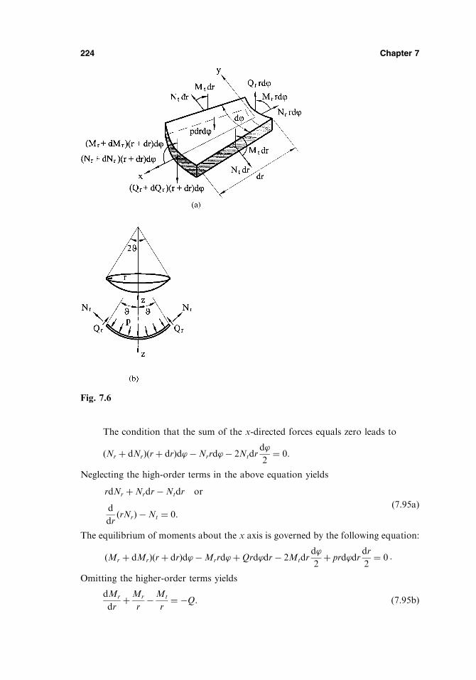
The condition that the sum of the x-directed forces equals zero leads to

Nr þ dNrð Þ rþ drð Þd’�Nrrd’� 2Ntdrd’

2¼ 0:

Neglecting the high-order terms in the above equation yields

rdNr þNrdr�Ntdr or

d

drrNrð Þ �Nt ¼ 0:

ð7:95aÞ

The equilibrium of moments about the x axis is governed by the following equation:

Mr þ dMrð Þ rþ drð Þd’�Mrrd’þQrd’dr� 2Mtdrd’

2þ prd’dr

dr

2¼ 0 :

Omitting the higher-order terms yields

dMr

drþMr

r�Mt

r¼ �Q: ð7:95bÞ

224 Chapter 7

Fig. 7.6

where

r2w ¼ 1

r

d

drrdw

dr

� �ð7:106Þ

is the Laplace operator in the polar coordinates for axisymmetric deformation.Let us express the strain components in terms of the stress function �. We

obtain

"r ¼1

Eh

1

r

d�

dr� � d

2�

dr2

!; "t ¼

1

Eh

d2�

dr2� �

r

d�

dr

!: ð7:107Þ

Introducing the above relations into the compatibility equation (7.93), one obtains

d3�

dr3þ 1

r

d2�

dr2� 1

r2d�

dr¼ �Eh

2

dw

dr

� �2

: ð7:108Þ

Applying again the Laplace operator (7.106), we can rewrite the above equation, asfollows:

d

drr2�� ¼ �Eh

2r

dw

dr

� �2

: ð7:109Þ

Thus, the governing differential equations for an axisymmetrically loaded, flexiblecircular plate have the following form

Dd

drr2w� � ¼ �þ 1

r

d�

dr

dw

dr; ð7:110aÞ

d

drr2�� ¼ �Eh

2r

dw

dr

� �2

: ð7:110bÞ

For the small-deflection stiff, axisymmetrically loaded circular plates, Eq. (7.110b) isomitted and Eq. (7.110a) appears in the form

Dd

drr2w� � ¼ �: ð7:111Þ

Differentiating both parts of this equation with respect to r, one obtains Eq. (4.17),as expected. On the contrary, for an absolutely flexible plate (i.e., membrane), theterm containing D should be neglected and we obtain the following system of differ-ential equations:

1

r

d�

dr

dw

dr¼ ��; ð7:112aÞ

d

drr2�� ¼ �Eh

2r

dw

dr

� �2

: ð7:112bÞ

Let us consider now the boundary conditions for flexible circular plates,described by Eqs (7.110). If a circular plate is simply supported along edge r ¼ a,then the boundary conditions are

w ¼ 0jr¼a;d2w

dr2þ �

r

dw

dr

!¼ 0jr¼a: ð7:113aÞ

226 Chapter 7

where f is the maximum deflection at the plate center, i.e., at r ¼ 0. Note that thisequation corresponds to the solution of the same problem for stiff circular platesaccording to the small-deflection plate bending theory (see Sec. 4.3).

Substituting for w from Eq. (a) into Eq. (7.110b), gives

d

drr2�� ¼ � 8Ehf 2

a2r

r

a� r3

a3

!2

:

Integrating this equation, one obtains

r2� ¼ � 8Ehf 2

a2r2

2a2� r4

2a4þ r6

6a6

!þ C1:

Multiplying this equation by r and integrating repeatedly, we obtain

d�

dr¼ � 2Ehf 2

a

r3

2a3� r5

3a5þ r7

12a7

!þ C1

r

2þ C2

1

r: ðbÞ

The constant C2 ¼ 0 due to the condition (7.118). The constant C1 is evaluated fromboundary conditions on the plate edge. We consider below two types of possibleboundary conditions for function �.

(a) Points of the plate edge are free to displace in the plane of the middle surfaceUsing the condition (7.117), one finds

C1 ¼Ehf 2

r2: ðcÞ

Then, we obtain

d�

dr¼ Ehf 2

6a3r

a� 6

r3

a3þ 4

r5

a5� r7

a7

!: ðdÞ

Since p ¼ p0 ¼ const, the function � in (7.98) is shown next:

� ¼ p0r

2:

On the other hand,

r2w ¼ � 8f

a21� 2

r2

a2

!:

Hence,

d

drr2w� � ¼ 32fr

a4: ðeÞ

Let us apply the Galerkin method in the form of the principle of virtual work (seeSec. 6.5) to solving Eq. (7.110a). In this case, the differential operator of the problemis of the form

Dd

drðr2wÞ �� 1

r

d�

dr

dw

dr:

228 Chapter 7

It has a sense of bending moments in dimension. Seeking the deflected surface of theplate in the form of the series

w ¼XNi¼1

Ai iðrÞ; ðfÞ

we can represent the Galerkin equation (6.39), according to the principle of virtualwork for solving Eq. (7.110a), as follows

ða0

EðwNÞd jdr

rdr ¼ 0; j ¼ 1; 2; . . . ;N: ðgÞ

Retaining only one term in the expansion (f) and setting according to (a),

1 ¼ 1� r2

a2

!2

:

Hence, the function Eðw1Þ is equal to

E1ðwÞ ¼ D32fr

a4� p0r

2þ 2

3

Eh

rf 3

5� 3�

1� �r

a

�� 6

r3

a3þ 4

r5

a5� r7

a7

!r

a� r3

a3

!:

Introducing the dimensionless variable

� ¼ r

a;

and substituting for E and 1 from the above equations into Eq. (g), one obtains

ð10

32Df �� 1

2p0�a

4 þ 2

3

Eh

�f 3

5� 3�

1� � �� 6�3 þ 4�5 � �7� �

�� 3� �� d� ¼ 0:

Evaluating this integral, we obtain the following equation:

6

7�3 þ 16

3ð1� �2Þ � ¼ p ; ðhÞ

where

� ¼ f

h; p ¼ p0

E

a

h

� �4: ðiÞ

For � ¼ 0:3, the above equation appears in the form

0:857�3 þ 5:862� ¼ p :

Solving this equation, gives �. Having determined �, we can determine the deflec-tions, bending moments, and normal stresses. The bending moments can be deter-mined from Eqs (4.14) by substituting for w from Eq. (a). We have

Mr ¼ 4Df

a2ð1þ �Þ � ð3þ �Þ�2� �

; ðjÞ

Mt ¼ 4D ð1þ �Þ � ð1þ 3�Þ�2� �: ðkÞ

Advanced Topics 229

The in-plane normal stresses, �r0 and �t0, are given by

�r0 ¼Nr

h¼ 1

hr

d�

dr; �t0 ¼

Nt

h¼ 1

h

d2�

dr2;

or substituting for d�=dr from Eq. (b), and (c), and determining d2�=dr2, we obtain

�r0 ¼Ef 2

6a23� 6�2 þ 4�4 � �6� �

;

�t0 ¼Ef 2

6a23� 18�2 þ 20�4 � 7�6� �

:

ðlÞ

It is seen from the above equations that, near the plate edge, the tangential stresses�t0 are compressive.

The bending normal stresses, �rb and �tb, are shown next:

�rb ¼6Mr

h2; �tb ¼

6Mt

h2:

At the plate center, the bending normal stresses are (for � ¼ 0:3Þ� rb ¼ � tb ¼ 2:86�; ðmÞ

and near the plate edge the above stresses are

� rb ¼ 4:4�; � tb ¼ 1:32�; ðnÞwhere

� rb ¼�rbE

a

h

� �2; � tb ¼

�tbE

a

h

� �2: ðoÞ

(b) The edge points are not displaced in the radial directionFrom Eq. (7.116), it follows that the constant C1 in Eq. (b) is equal to

C1 ¼Ehf 2

3a25� 3�

1� � ;

from which

d�

dr¼ Ehf 2

6a

5� 3�

1� � �� 6�3 þ 4�5 � �7� �

:

In this case of the boundary conditions, the Galerkin equation (6.39) is of the form

ð10

32Df �� 1

2p0�a

4 þ 2

3

Ehf 3

�

5� 3�

1� � �� 6�3 þ 4�5 � �7� �

ð�� 3Þ" #

ð�� 3Þ�d� ¼ 0:

Evaluating this integral, yields the following equation:

2

21

23� 9�

1� � �3 þ 16

3ð1� �2Þ � ¼ p ; ðpÞ

or for � ¼ 0:3;

230 Chapter 7

" kð Þx ¼ �zk

@2w

@x2; " kð Þ

y ¼ �zk@2w

@y2; � kð Þ

xy ¼ �2zk@2w

@x@yð7:119Þ

From Hooke’s law, Eqs (2.9), we obtain

� kð Þx ¼ Ek

1� �2k" kð Þx þ �k" kð Þ

y

� �; � kð Þ

y ¼ Ek

1� � kð Þk

" kð Þy þ �k" kð Þ

x

� �;

� kð Þxy ¼ Ek

2 1þ �kð Þ �kð Þxy :

ð7:120Þ

Substituting the strains defined by Eqs (7.119) into the above, integrating over eachlayer and summing the results, we obtain the following bending and twistingmoments:

Mx

My

Mxy

8><>:

9>=>; ¼

Xk

ðzkzk�1

�x

�y

�xy

8><>:

9>=>;

kð Þ

zdz: ð7:121Þ

The stress components defined in the kth layer can be calculated from

� kð Þx ¼ �zk

Ek

1� �2k@2w

@x2þ �k

@2w

@y2

!; � kð Þ

y ¼ �zkEk

1� �2k@2w

@y2þ �k

@2w

@x2

!;

� kð Þxy ¼ �zk

Ek

1þ �k@2w

@x@y:

ð7:122ÞThe governing differential equation for multilayered plates can be derived similarly,as described in Sec. 2.4. This equation will be similar to that for homogeneous plates,but replacing the rigidity D by the so-called transformed rigidity, Dt, of the multi-layered plates, as follows [22,23]:

Dtr2r2w x; yð Þ ¼ p x; yð Þ; ð7:123Þwhere Dt is given by Pister and Dong in the form [22]

Dt ¼AC � B2

A; ð7:124Þ

and the constants A;B; and C are given by

A ¼Xk

Ek

1� �2kzk � zk�1ð Þ;B ¼

Xk

Ek

1� �2kz2k � z2k�1

2

!;

C ¼Xk

Ek

1� �2kz3k � z3k�1

3

!:

ð7:125Þ

The deflected surface of the multilayered plates can be determined by the sameanalytical and numerical methods as those discussed for homogeneous plates inChapters 3, 4, and 6.

232 Chapter 7

The twist, @2w=@x@y, is also made up of the components due to the twisting moment,Mxy, and that due to the variation of the shear forces, Qx and Qy. The differentialequation of the twist curvature is given by

@2w

@x@y¼ �Mxy

Dxy

þ 1

2

1

DQx

@Qx

@yþ 1

2

1

DQy

@Qy

@x: ð7:128bÞ

It is convenient to invert Eqs (7.128) as follows:

Mx ¼ �D x

@

@x

@w

@x� Qx

DQx

� �þ �y

@

@y

@w

@y� Qy

DQy

!" #;

My ¼ �D y

@

@y

@w

@y� Qy

DQy

!þ �x

@

@x

@w

@x� Qx

DQx

� �" #;

Mxy ¼ �Dxy

2

@

@x

@w

@y� Qy

DQy

!þ @

@y

@w

@x� Qx

DQX

� �" #;

ð7:129Þ

where

D x ¼

Dx

1� �x�y; D

y ¼Dy

1� �x�y: ð7:130Þ

Substituting the relations (7.129) into the equilibrium equations, Eqs (2.19)–(2.22),one finds

ðDxy þ �yD xÞ@3w

@x@y2þD

x

@3w

@x3¼ D

x

DQx

@2Qx

@x2þ 1

2

Dxy

DQx

@2Qx

@y2

þ 1

2

Dxy

DQy

þ �yD x

DQy

!@2Qy

@x@y�Qx; ð7:131aÞ

Dxy þ �xD y

� � @3w@x2@y

þD y

@3w

@y3¼ D

y

DQy

@2Qy

@y2þ 1

2

Dxy

DQy

@2Qy

@x2

þ 1

2

Dxy

DQx

þ �xD y

DQx

� �@2Qx

@x@y�Qy; ð7:131bÞ

@Qx

@xþ @Qy

@y¼ �p: ð7:131cÞ

This is the system of the governing differential equations in w;Qx; and Qy for thesmall-deflection theory of sandwich plate bending problems based on the assumptionsintroduced earlier.

Assuming general values for the middle surface deflection w and the shearforces Qx and Qy, which satisfy Eqs (7.131) and the relevant boundary conditions,it is possible to solve a number of bending problems of sandwich plates. The bound-ary conditions on the edges of the sandwich plate should be consistent with Eqs(7.131). We present below a simplified variant of the boundary conditions: namely,

Advanced Topics 235

236 Chapter 7

(a) Simply supported edge (y ¼ const) in which all points in the boundary are pre-vented from moving parallel to the edge.

w ¼ 0; My ¼ 0;Qx

DQx

¼ 0: ð7:132aÞ

(b) Free edge (y ¼ constÞMy ¼ 0; Mxy ¼ 0; Qy ¼ 0: ð7:132bÞ

(c) Clamped edge (y ¼ const) in which the points in the boundary are prevented frommoving parallel to the edge.

w ¼ 0;Qx

DQx

¼ 0;@w

@y� Qy

DQy

¼ 0: ð7:132cÞ

Similarly, the boundary conditions may be formulated on edges x ¼ const.Let us consider a special case of the sandwich plate having isotropic faces of

equal thicknesses and an isotropic non-direct stress-carrying core. For this special case,assuming that t � c, we have

D x ¼ D

y ¼ Ds ¼Ef td

2

2ð1� �2f Þ; �x ¼ �y ¼ �f ;

DQx¼ DQy

¼ DQ ¼ Gc

d2

c; Dxy ¼ Dsð1� �f Þ;

ð7:133Þ

where Ef and �f are the modulus of elasticity and Poisson’s ratio, respectively, ofisotropic sandwich plate faces; Gc is the modulus of rigidity of the isotropic core; d ¼cþ t is the distance between the centerlines of the faces; Ds and DQ are the flexuraland transverse shear stiffnesses of the isotropic sandwich plate.

For this special case, the system of the three governing differential equations(7.131) can be reduced to a single equation. In fact, the equations of equilibrium (Eqs(2.19)–(2.22)) are reduced to Eq. (2.23). Substituting for Mx;My; and Mxy from Eqs(7.129) into Eq. (2.23) and taking into account the relations (7.133), one obtains

Dsr2r2w� Ds

DQ

@3Qx

@x3þ @

3Qy

@y3þ @3Qx

@x@y2þ @3Qy

@x2@y

!¼ p: ð7:134Þ

It can be easily verified that the following equality takes place:

@3Qx

@x3þ @

3Qy

@y3þ @3Qx

@x@y2þ @3Qy

@x2@y¼ r2 @Qx

@xþ @Qy

@y

� �¼ �r2p:

Thus, Eq. (7.134) finally can be rewritten in the following form:

Dsr2r2w ¼ 1� Ds

DQ

r2

� �p: ð7:135Þ

This is the governing differential equation of the isotropic sandwich plate. In the limit-ing case when Gc ! 1, Eq. (7.135) is reduced to the governing differential equationof isotropic homogeneous plate bending, Eq. (2.24) with the flexural stiffness Ds, i.e.,with the stiffness of the composed section consisting of the two layers of thickness teach and separated by a distance c. In another limiting case when Gc ! 0, Eq.(7.135) is reduced to the corresponding equation for the separated faces.

Here only basic concepts have been given of the theory of sandwich plates. Theinterested reader is referred to Refs [24–28].

Advanced Topics 239

REFERENCES

1. Boley, B.A. and Weiner, J.H., Theory of Thermal Stresses, John Wiley and Sons, New

York, 1960.

2. Johns, D.J., Thermal Stress Analysis, Pergamon Press, Elmsford, New York, 1965.

3. Lekhnitskii, S.G., Anisotropic Plates, Gordon and Breach, New York, 1968.

4. Timoshenko, S.P and Woinowski-Krieger S., Theory of Plates and Shells, 2nd. edn,


5. Boyarshinov SV., The Fundamentals of Structural Mechanics of Machines,

Mashinostroenie, Moscow, 1973 (in Russian).

6. Troitsky, M.S., Orthotropic Bridges – Theory and Design, The James Lincoln Arc

Welding Foundation, Cleveland, 1987.

7. Huffington, H.J., Theoretical determination of rigidity properties of orthotropic stiffened

plates, J Appl Mech, vol. 23, No. 1, pp. 15–20 (1956).

8. Donnel, L.H., Beams, Plates, and Shells, McGraw-Hill, New York, 1976.

9. Alfutov, N.A., On paradoxes of the theory of thin elastic plates,Mechanics of Solids, No.

3, pp. 65–72 (1992).

10. Reissner, E., On the theory of bending of elastic plates, J Math Phys, vol. 23, 184–191

(1944).

11. Reissner, E., The effect of transverse shear deformation on the bending of elastic plates, J

Appl Mech, vol. 12, pp A69–A77 (1945).

12. Vasil’ev, V.V., Classical theory of plates: historical perspective and state-of-the-art,

Mechanics of Solids, vol. 33, No. 3, pp. 35–45 (1998).

13. Zihlin, P.A., On Poisson’s and Kirchhoff’s theories of plates from the point of view of

the modern theory of plates, Mechanics of Solids, No. 3, pp. 65–72 (1992).

14. Green, A., On Reissner’s theory of bending of elastic plates, Quart Appl Math, vol. 7,

No. 2, pp. 223–228 (1949).

15. Mindlin, R.D., Influence of rotary inertia and shear on flexural motions of isotropic

elastic plates, J Appl Mech, vol. 18, No.1, pp. 31–38 (1951).

16. Reddy, J.N., Energy and Variational Methods in Applied Mechanics, John Wiley and

Sons, New York, 1984.

17. Von Karman, Th., Encyklop. die der Mathematischen, Wissenschaften, vol .IV, 1910.

18. Levy, S., Large deflection theory for rectangular plates, Proc. Symp. on Non-Linear

Problems, Symp Appl Math., I, pp. 197–210 (1947).

19. Volmir, A.S., Flexible Plates and Shells, AFFDL-TR-66-216, Air Force Flight Dynamics

Laboratory, Wright-Patterson Air Force Base, Ohio, 1967.

20. Zienkiewitcz, D.C., The Finite Element Method, McGraw-Hill, New York, 1977.

21. Alexandrov, A.P. and Potapov, V.D., The Fundamentals of the Theory of Elasticity and

Plasticity, Izd-vo ‘‘Vyshaia Shkola,’’ Moscow, 1990 (in Russian).

22. Pister, K.S. and Dong, S.B., Elastic bending of layered plates, Proc ASCE J Eng Mech

Div, October, 84, pp. 1–10 (1950).

23. Ambartsumyan, S.A., Theory of Anisotropic Plates (translation from the Russian),

Technomic, Stamford, CT, 1970.

24. Libove, C. and Butdorf, S.B., A General Small-Deflection Theory for Flat Sandwich

Plates, NACA TN 1526, 1948.

25. Robinson, J.R., The buckling and bending of orthotropic sandwich plates with all edges

simply supported, Aeronautical Quart, vol. 6, No. 2, pp. 125–148 (1955).

26. Libove, C. and Hubka, R.E., Elastic Constants for Corrugated Core Sandwich Plates,

NACA TN 2289, 1951.

27. Allen, H.G., Analysis and Design of Structural Sandwich Panels, Pergamon Press,

London, 1969.

28. Plantema, F.J., Sandwich Construction, John Wiley and Sons, New York, 1966.

8

Buckling of Plates

8.1 INTRODUCTION

Thin plates of various shapes used in naval and aeronautical structures are oftensubjected to normal compressive and shearing loads acting in the middle plane of theplate (in-plane loads). Under certain conditions such loads can result in a platebuckling. Buckling or elastic instability of plates is of great practical importance.The buckling load depends on the plate thickness: the thinner the plate, the lower isthe buckling load. In many cases, a failure of thin plate elements may be attributedto an elastic instability and not to the lack of their strength. Therefore, plate buck-ling analysis presents an integral part of the general analysis of a structure.

In this chapter, we consider a systematic but simplified analysis of plate buck-ling and obtain some useful relations between the critical loads and plate parameters.

8.2 GENERAL POSTULATIONS OF THE THEORY OF STABILITY OFPLATES

This section contains some fundamentals of classical stability analysis of thin elasticplates. It should be noted that the stability analysis of plates is qualitatively similarto the Euler stability analysis of columns [1].

Consider an ideal thin, elastic plate which is assumed initially to be perfectlyflat and subjected to external in-plane compressive and shear loads acting strictly inthe middle plane of the plate. The resulting deformations of this plate are character-ized by the absence of deflections (u 6¼ 0; v 6¼ 0; and w ¼ 0) and, consequently, of thebending and twisting moments, as well as the transverse shear forces. Such a planestress condition of the plate is referred to as an initial or flat configuration of equili-brium, assuming the equilibrium conditions between applied external loads and thecorresponding in-plane stress resultants.

241

ing the critical loads, by the Ritz method (see Sec. 6.6). In this case, the deflectionsurface of the plate, w x; yð Þ, in the neighboring state of equilibrium is sought in theform of Eq. (6.42). If all external forces acting on the plate vary in the proportion toa load parameter �, then substituting Eq. (6.42) into the condition (8.5a) yields

�� ¼ �� ;C1;C2; . . . ;Cnð Þ ¼ 0; ð8:5bÞ

where Ci i ¼ 1; 2; . . . ;Cnð Þ are undetermined coefficients. Numerical implementationof the conditions (8.5) requires the usual minimization process (Eq. (6.44)). Thelatter also leads to a system of linear algebraic, homogeneous equations. So, apply-ing the procedure discussed earlier for determining a nontrivial solution in the equi-librium method, we can find all the characteristic numbers �i, and their smallestvalue corresponding to the critical eigenvalue, �cr.

Dynamic or kinematic method

This method is the most general and universal and is associated with the mathema-tical problem of the stability of motion. The method is based on examining trans-verse oscillations of a thin plate subjected to in-plane edge loads. The smallest valueof the load that results in unbounded growth of the amplitude of these oscillations intime is considered as a critical value of the applied loads.

The equilibrium and energy methods are now discussed in more detail.

8.3 THE EQUILIBRIUM METHOD

8.3.1 Buckling of rectangular plates

According to the equilibrium method, the critical values of applied in-plane forcesmay be found from the solution of the governing differential equation (8.1) or itsequivalent analog (8.3). As mentioned in Sec. 8.2, this equation is a homogeneous,linear partial differential equation with, generally speaking, variable coefficients. It isimpossible to find its analytical solution in the general case. However, for someparticular but practically important cases this equation makes it possible to obtainan exact solution. The following examples illustrate the equilibrium method forobtaining the exact solutions associated with determining the critical forces in rec-tangular plates.

Example 8.1

Determine the critical buckling load for a simply supported plate subjected to auniformly distributed compressive edge load qx acting in the x direction, as shownin Fig. 8.1.

Solution

For this particular case Nx ¼ �qx and Ny ¼ Nxy ¼ 0. The differential equation (8.1)becomes

Dr2r2wþNx

@2w

@x2¼ 0: ð8:6Þ

Buckling of Plates 245

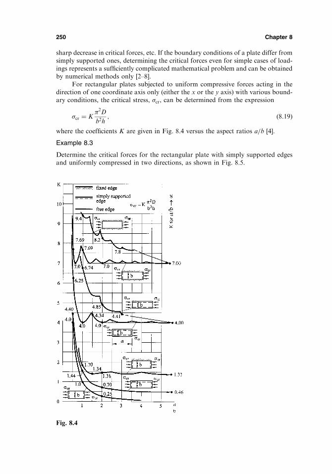
sharp decrease in critical forces, etc. If the boundary conditions of a plate differ fromsimply supported ones, determining the critical forces even for simple cases of load-ings represents a sufficiently complicated mathematical problem and can be obtainedby numerical methods only [2–8].

For rectangular plates subjected to uniform compressive forces acting in thedirection of one coordinate axis only (either the x or the y axis) with various bound-ary conditions, the critical stress, �cr, can be determined from the expression

�cr ¼ K�2D

b2h; ð8:19Þ

where the coefficients K are given in Fig. 8.4 versus the aspect ratios a=b [4].

Example 8.3

Determine the critical forces for the rectangular plate with simply supported edgesand uniformly compressed in two directions, as shown in Fig. 8.5.

250 Chapter 8

Fig. 8.4

Denoting

�2 ¼ qrD; ð8:28Þ

and using the relations between the polar and Cartesian coordinates, Eqs (4.1)–(4.4),we obtain the following differential equation of the axisymmetrically loaded circularplate subjected to in-plane compressive forces qr:

d4w

dr4þ 2

r

d3w

dr3� 1

r2d2w

dr2þ 1

r3dw

drþ �2 d2w

dr2þ 1

r

dw

dr

" #¼ 0: ð8:29Þ

Let us introduce the following new variable:

� ¼ �r; ð8:30Þwhich represents a dimensionless polar radius. Using the new variable �, we canrewrite Eq. (8.29), as follows:

d4w

d�4þ 2

�

d3w

d�3þ 1� 1

�2

� �d2w

d�2þ 1

�1þ 1

�2

� �dw

d�¼ 0: ð8:31Þ

This is a fourth-order linear, homogeneous differential equation. The general solu-tion of this equation is given by [1] as

w �ð Þ ¼ C1 þ C2 ln �þ C3J0 �ð Þ þ C4Y0 �ð Þ; ð8:32Þwhere J0 �ð Þ and Y0 �ð Þ are the Bessel functions of the first and second kind of zeroorders, respectively. They are tabulated in Ref. [10]. In Eq. (8.32), Ci i ¼ 1; . . . ; 4ð Þare constants of integration. Since w �ð Þ must be finite for all values of �; including�¼ 0, then the two terms ln � and Y0 �ð Þ, having singularities at � ¼ 0, must bedropped for the solid plate because they approach an infinity when �! 1. Thus,for the solid circular plate, Eq. (8.32) must be taken in the form

w �ð Þ ¼ C1 þ C3J0 �ð Þ: ð8:33ÞDetermine the critical values of the radial compressive forces, qr, applied to themiddle plane of solid circular plates for two types of boundary supports.


Fig. 8.6

is simplified and has the following form for the above-mentioned increment of themiddle surface:

�U ¼ 1

2

ð ðV

ð�x"x þ �y"y þ �xy�xy� �

dV : ðaÞ

This increment of the strain energy can also be expressed in terms of the in-planestress resultants. The latter are related to the stress components as follows:

�x ¼Nx

h; �y ¼

Ny

h; and �xy ¼

Nxy

h: ðbÞ

Substituting the above into Eq. (a) and integrating over the plate thickness, h, resultsin the following expression for the increment in the strain energy of the plate middlesurface:

�U0 ¼ð ð

A

Nx"x þNy"y þNxy�xy� �

dxdy: ð8:40Þ

Note that there is no 1/2 coefficient in Eq. (8.40), since the in-plane stress resultantsare already acting when additional middle surface strains (due to the buckling)occur. For the sake of simplicity, we derive the expression for �U0 for a rectangularplate of dimensions a b. Inserting Eqs (7.82) into Eq. (8.40) results in the followingexpression for the increment of the strain energy of the plate middle surface:

�U0 ¼ðb0

ða0

Nx

@u

@xþNy

@v

@yþNxy

@u

@yþ @v

@x

� �� dxdy

þ 1

2

ðb0

ðb0

Nx

@w

@x

� �2

þNy

@w

@y

� �2

þ2Nxy

@w

@x

@w

@y

" #dxdy:

ð8:41Þ

We transform the first integral of the right-hand side of Eq. (8.41). Integrating thisexpression term-by-term, we obtain

ðb0

ða0

Nx

@u

@xþNy

@v

@yþNxY

@u

@yþ @v

@x

� �� dxdy ¼

ðb0

Nxu a

0þ Nxyv a

0

h idy

þðb0

Nyv b

0þ Nxyu b

0

h idx�

ðb0

ða0

u@Nx

@xþ @Nxy

@y

� �dxdy

�ðb0

ða0

v@Nxy

@xþ @Ny

@y

� �dxdy:

ð8:42Þ

Using Eqs (3.90a) and (3.90b), we can conclude that the two last integrals onthe right-hand side in the above expression vanish. The first two integrals on theright-hand side of Eq. (8.42) represent the work, We, done by the in-plane externalforces applied to the middle surface of the plate. Thus, the expression (8.42) can berepresented in the form

256 Chapter 8

�U0 ¼ We þ1

2

ðb0

ða0

Nx

@w

@x

� �2

þNy

@w

@y

� �2

þ2Nxy

@w

@x

@w

@y

" #dxdy: ð8:43Þ

It can be shown that the expression for �U0 in the form of Eq. (8.43) is valid(replacing the limits of integration) for a plate of any geometry, not necessarily,rectangular.

The increment in the potential of the external, in-plane forces applied to theplate is equal to the negative value of the work done by these forces, i.e.,

�� ¼ �We: ð8:44ÞThe strain energy of the bending and twisting of a plate, Ub, is given by Eq. (2.53).Therefore, the increment in the total potential energy of the plate upon buckling,��, can be obtained by substituting Eqs (2.53) and (8.43) with taking into accountEq. (8.44) on the right-hand side of Eq. (8.4).

�� ¼ 1

2

ð ðA

D@2w

@x2þ @

2w

@y2

!2

þ2 1� �ð Þ @2w

@x@y

!2

� @2w

@x2@2w

@y2

24

35

8<:

9=;dxdy

þ 1

2

ð ðA

Nx

@w

@x

� �2

þNy

@w

@y

� �2

þ2Nxy

@w

@x

@w

@y

" #dxdy

ð8:45Þ

As mentioned in Sec. 8.2, the energy criterion (8.5) may be employed be obtain theexact and approximate solutions of the plate buckling problems. In the latter case,this criterion may be combined with, for instance, the Ritz method together with theeigenvalue technique introduced in Sec. 8.2.

Note that in practice �� ¼ 0 only if the form chosen for the deflection is exact.Any approximation form, when Eq. (8.45) is applied, will give a value of the criticalforce higher than the true value. Let us demonstrate the advantages of the energycriterion in illustrative examples.

Example 8.4

Using the Ritz method, determine the critical buckling load for the plate with threesimply supported edges x ¼ 0; a and y ¼ 0 and one free edge y ¼ b, as shown in Fig.8.7. The plate is loaded by linearly distributed compressive in-plane forcesqx ¼ q 1þ y

b

� �along the simply supported edges x ¼ 0; a, where > 0 is some fixed

parameter.

Solution

The deflection surface of the plate can be approximated, as follows:

w ¼ sinn�x

a

XNi¼1

Ciyi: ðaÞ

This approximate solution satisfies exactly the prescribed geometric boundary con-ditions, i.e.,

w ¼ 0jx¼0;a; w ¼ 0jy¼0: ðbÞ

Retaining only one term (i ¼ 1) in the series (a), we can find the following:


@w

@x¼ C1y

n�

acos

n�x

a

� �;@2w

@x2¼ �C1y

n�

a

� �2sin

n�x

a;

@2w

@x@y¼ C1

n�

acos

n�x

a

� �;@2w

@y2¼ 0:

For this type of loading, the solution of the plane stress problem is Nx ¼ �qx,Ny ¼ Nxy ¼ 0. Substituting the above into Eq. (8.45), and performing the operationsof integration, we obtain

�� ¼ C21

ab

4D

b2

3

n�

a

� �4þ2 1� �ð Þ n�

a

� �2" #� q

n�

a

� �2b2

1

3þ

4

� �( ):

The eigenvalues of the load qx can be found from equation @�=@C1 ¼ 0. We have

qn ¼n2�2D

b2b2=a2 þ 6 1� �ð Þ=n2�2

1þ 3 =4

" #:

For n ¼ 1, the smallest eigenvalue is approximately equal to the critical value, i.e.,

qcr ¼b2=a2 þ 6 1� �ð Þ=�2

1� 3 =4� �

2D

b2: ð8:46Þ

Example 8.5

Determine the critical value of uniformly distributed in-plane shear forces qxy for thesimply supported rectangular plate shown in Fig. 8.8.

Solution

We assume that the deflection surface is adequately approximated as follows:

w ¼ C1 sin�x

asin�y

bþ C2 sin

2�x

asin

2�y

b; ðaÞ

where C1 and C2 are two unknown coefficients. It is obvious that w in the form of (a)satisfies exactly the prescribed geometrical boundary conditions (w ¼ 0 on theboundary).

258 Chapter 8

Fig. 8.7

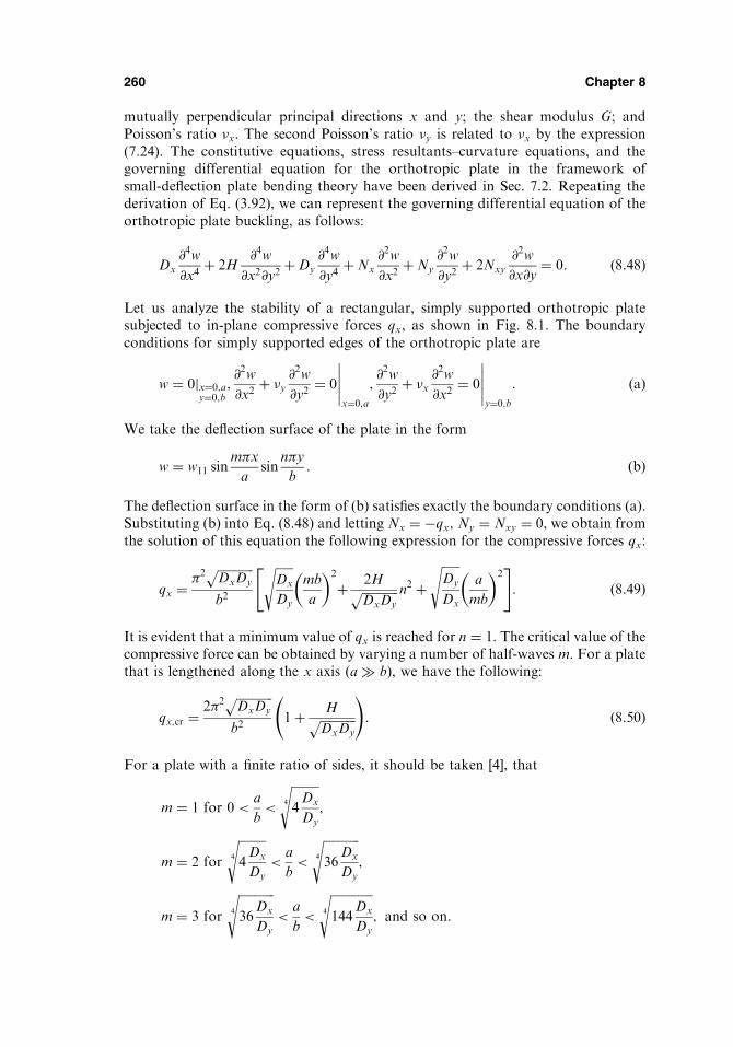
mutually perpendicular principal directions x and y; the shear modulus G; andPoisson’s ratio �x. The second Poisson’s ratio �y is related to �x by the expression(7.24). The constitutive equations, stress resultants–curvature equations, and thegoverning differential equation for the orthotropic plate in the framework ofsmall-deflection plate bending theory have been derived in Sec. 7.2. Repeating thederivation of Eq. (3.92), we can represent the governing differential equation of theorthotropic plate buckling, as follows:

Dx

@4w

@x4þ 2H

@4w

@x2@y2þDy

@4w

@y4þNx

@2w

@x2þNy

@2w

@y2þ 2Nxy

@2w

@x@y¼ 0: ð8:48Þ

Let us analyze the stability of a rectangular, simply supported orthotropic platesubjected to in-plane compressive forces qx, as shown in Fig. 8.1. The boundaryconditions for simply supported edges of the orthotropic plate are

w ¼ 0jx¼0;ay¼0;b

;@2w

@x2þ �y

@2w

@y2¼ 0

x¼0;a

;@2w

@y2þ �x

@2w

@x2¼ 0

y¼0;b

: ðaÞ

We take the deflection surface of the plate in the form

w ¼ w11 sinm�x

asin

n�y

b: ðbÞ

The deflection surface in the form of (b) satisfies exactly the boundary conditions (a).Substituting (b) into Eq. (8.48) and letting Nx ¼ �qx; Ny ¼ Nxy ¼ 0, we obtain fromthe solution of this equation the following expression for the compressive forces qx:

qx ¼ �2ffiffiffiffiffiffiffiffiffiffiffiffiDxDy

pb2

ffiffiffiffiffiffiDx

Dy

smb

a

� �2

þ 2HffiffiffiffiffiffiffiffiffiffiffiffiDxDy

p n2 þffiffiffiffiffiffiDy

Dx

sa

mb

� �2" #

: ð8:49Þ

It is evident that a minimum value of qx is reached for n ¼ 1. The critical value of thecompressive force can be obtained by varying a number of half-waves m. For a platethat is lengthened along the x axis (a � b), we have the following:

qx;cr ¼2�2

ffiffiffiffiffiffiffiffiffiffiffiffiDxDy

pb2

1þ HffiffiffiffiffiffiffiffiffiffiffiffiDxDy

p !

: ð8:50Þ

For a plate with a finite ratio of sides, it should be taken [4], that

m ¼ 1 for 0 <a

b<

ffiffiffiffiffiffiffiffiffi4Dx

Dy

4

s;

m ¼ 2 for

ffiffiffiffiffiffiffiffiffi4Dx

Dy

4

s<

a

b<

ffiffiffiffiffiffiffiffiffiffiffiffi36

Dx

Dy

4

s;

m ¼ 3 for

ffiffiffiffiffiffiffiffiffiffiffiffi36

Dx

Dy

4

s<

a

b<

ffiffiffiffiffiffiffiffiffiffiffiffiffiffi144

Dx

Dy

4

s; and so on:

260 Chapter 8

Substituting the above into Eq. (8.6) and letting Nx ¼ �qx; Ny ¼ 0;Nxy ¼ 0, gives

d4F yð Þdy4

� 2m�

a

� �2d2F yð Þdy2

þ m�

a

� �2 m�

a

� �2� qx

D

� �F yð Þ ¼ 0: ð8:52Þ

Its solution is of the form

F yð Þ ¼ C1 coshyþ C2 sinh yþ C3 cosyþ C4 sin y; ð8:53Þwhere

¼ffiffiffiffiffiffiffiffiffiffiffiffiffiffiffiffiffiffiffiffiffiffiffiffiffiffiffiffi� �þ

ffiffiffiffiffiqxD

r� �s; ¼

ffiffiffiffiffiffiffiffiffiffiffiffiffiffiffiffiffiffiffiffiffiffiffiffiffiffiffiffi�

ffiffiffiffiffiqxD

r� �

� �sand � ¼ m�

a: ð8:54Þ

The boundary conditions on the edge y ¼ b=2 are

w ¼ 0;@2w

@y2¼ 0

y¼b=2

: ð8:55Þ

Assume that the plate is buckled together with the rib; then the bent surface of theplate must be symmetric about the line y ¼ 0. This results in the following condition:

@w

@y¼ 0

y¼0

: ð8:56Þ

The difference in the reaction forces from the two strips of the plate given by theexpression

Ry ¼ �D@3w

@y3þ 2� �ð Þ @

3w

@y@x2

" #ð8:57Þ

will be transmitted to the rib. Assume that the plate and rib are made of one and thesame material. Due to the assumption adopted above for deformations of the rib, itcan be easily shown that only the first term in the brackets of Eq. (8.57) should betaken into account. If we assume that the rib together with the plate is subjected to

262 Chapter 8

Fig. 8.9

the compressive forces qx, then the equation for the elastic curve of the rib may berepresented in the form

EIi@4w

@x4þ qx

@2w

@x2þ 2D

@3w

@y3

!y¼0

¼ 0;

or replacing qx ¼ Nx ¼ �xAi for the rib, we obtain

EIi@4w

@x4þ �xAi

@2w

@x2þ 2D

@3w

@y3

!y¼0

¼ 0; ð8:58Þ

where Ii and Ai are the second moment of inertia and area of the rib cross section,respectively.

Let us introduce the following parameters:

� ¼ a

b; � ¼ EIi

Db; � ¼ Ai

bh: ð8:59Þ

Introducing Eq. (8.53) into the conditions (8.55), (8.56), and (8.58), we obtain asystem of linear algebraic homogeneous equations for C1; . . . ;C4. Equating thedeterminant of this system to zero, yields the following equation:

1

btanh

b

2� 1

btan

b

2

� ��m2

2� K�

!m2�2

2� 4

m

ffiffiffiffiK

p¼ 0; ð8:60Þ

where

K ¼ �x;cr�x;E

ð8:61Þ

and

�x;cr ¼qx;crh; �x;E ¼ 4

�2D

b2hð8:62Þ

where �x;E is the critical stress for a rectangular, simply supported, unstiffened platewith the dimensions of Fig. 8.9 (see Eq. (8.11)). Equation (8.60) may be solved by themethod of trial and errors. For m ¼ 1 and � > 2, its solution, using the parametersintroduced in Eqs (8.59), gives the following expression for �x;cr:

�x;cr ¼�2D

b2h

1þ �2� �2þ2�

�2 1þ 2�ð Þ : ð8:63Þ

Now we analyze the stability problems for stiffened plates by the energy method.

Example 8.7

Determine the critical value of the in-plane compressive forces qx acting on the platereinforced by two equally spaced stiffeners, as shown in Fig. 8.10. The plate is simplysupported on all edges. Let Ai and Bi (Bi ¼ EIi) be the area of the cross section andthe bending stiffness of a stiffener, and ci be spacing of the stiffeners.


qx;cr ¼�4D

b21þ �2� �þ 3�

�2 1� 3�ð Þ ; ð8:68Þ

where �; �; and � are given by formulas (8.59). The solution (8.68) is done in the firstapproximation, i.e., for m ¼ n ¼ 1. If a rectangular, simply supported plate is rein-forced by i equally spaced stiffeners then the critical value of the compressive forcesis the following:

qx;cr ¼�2D

b2

1þ �2� �2þ2Pi

�i sin2 �ci=bð Þ

�2 1þ 2Pi

�i sin2 �ci=bð Þ

� � : ð8:69Þ

8.6 POSTBUCKLING BEHAVIOR OF PLATES

8.6.1 Large deflections of plates in compression

Using the linearized buckling analysis introduced in Sec. 8.2, we have consideredonly the initial elastic buckling of flat plates and the critical forces and stresses havebeen found for some typical loadings and boundary conditions. The critical force isthe force at which bifurcation of equilibrium states occurs and is of fundamentalsignificance to the designer. So, the critical loads found in the previous sectionsrepresent merely the loads at which buckling begins. It should be noted that thepostbuckling behavior of plates is markedly different from that of thin rods. While asmall increase in the critical load for rods will produce a complete collapse, the load-carrying capacity of the plate is not exhausted and elastic plate can carry stresseshigher than �cr. It can be explained, first of all, by the effect of large deflections in thepostbuckling stage and, then, by the fact that the longitudinal edges of the plate areusually constrained to remain straight. Thus, the postbuckling mechanism of elasticplates is characterized not only by bending but also by the direct (or in-plane)stresses. It is important that the latter become comparable in magnitude with theformer stresses.

The use of an additional strength due to the postbuckling effects is of greatpractical importance in the design of ship and aerospace structures. By consideringthe postbuckling behavior of plates, considerable weight savings can be achieved. Inthese structures, the edges of the plates are usually supported by stringers in such away that they remain straight during buckling. After buckling, the central part of theplate bulges out, and an increasingly larger portion of the load is carried by thematerial close to the supported edges (stringers) of the plate.

The nonlinear, large-deflection plate bending theory, discussed in Sec. 7.4, canbe used for the analysis of the postbuckling behavior of plates. Because of a non-linearity of the governing differential equations of this analysis, the resulting math-ematical difficulties are considerable and exact solutions can very seldom beobtained. The most generally used techniques for the treatment of postbuckling ofplates are based on numerical methods [11,12].

For some simple cases an analytical solution can be obtained under someassumptions regarding the plate behavior, boundary conditions, etc. Consider arectangular, simply supported plate, as shown in Fig. 8.1. The plate is subjected to


As seen, the in-plane shear stresses are zero. Let us apply the Galerkin method tosolve Eq. (8.71b). Using the general procedure of the method discussed in Sec. 6.5,we obtainða

0

ðb0

E sin�x

asin�y

bdxdy ¼ 0; ð8:77Þ

where

E � D

hr4w� @2�

@y2@2w

@x2� @

2�

@x2@2w

@y2þ 2

@2�

@x@y

@2w

@x@y: ð8:78Þ

Substituting for w and � from Eqs (8.70) and (8.75) into (8.77) and performingthe corresponding operations of differentiation and integration, yields thefollowing:

D�4ab

4w11

1

a2þ 1

b2

� �2

� qxw11

�2

a2ab

4þ E

�4w311

64h

1

a4þ 1

b4

� �ab ¼ 0: ð8:79Þ

Assuming that w11 6¼ 0, we obtain

qx ¼ Nx ¼ �xh ¼ D�2

b2b

aþ a

b

� �2

þE�2h

16b2w211

b2

a2þ a2

b2

!: ð8:80Þ

Since the first term on the right-hand side of the above equation represents thecritical force of the linear buckling analysis, qx;cr, introduced in Sec. 8.3, it is evidentthat the plate can sustain a compression load greater than the linear buckling. Itshould be noted that the load-carrying capacity is more pronounced when theunloaded edges are constrained to remain straight (Ny 6¼ 0).

The first detailed analysis of the postbuckling behavior of plates loaded bycompressive loads was conducted by von Karman et al. [13], who suggested a sim-plified approach to obtain an estimate for the ultimate load carried by the buckledplate. Based on experimental observations, this simplified method assumes that theultimate buckling load of the plate is carried exclusively by two strips of equal width(the so-called effective width), located along the unloaded edges, and the stringers,jointly with the effective width portion of the plate, act as columns. A detailednumerical analysis of the postbuckling behavior of thin plates with various boundaryconditions using the simplified method based on the effective width concept incompression for routine design purposes was developed by Marguerre [14], Cox[2], Schade [15], etc. The interested reader is referred to these references and toRefs [1,3].

8.6.2 Load-carrying capacity of plates in compression

We have seen that a plate after buckling may carry in some cases a compressive forcethat is many times higher than the critical load at which buckling begins. So, in caseswhen issues of weight economy are of fundamental importance, as for example in theaircraft industry, it is expedient to determine not only the critical load but also theultimate load which the plate can carry without failure, which corresponds to theplate load-carrying capacity in compression.


We consider below a rectangular plate that is pin-connected along its edgeswith rigid stiffeners. The plate is subjected to compressive forces in one direction, asshown in Fig. 8.11a.

Prior to buckling of the plate, the compressive stresses are uniformly distrib-uted over its width, b, but after buckling the distribution of stresses along the loadededges becomes progressively nonlinear: they increase more intensively in the vicinityof the plate edges and the stresses differ little from their critical values in the centralpart of the plate. A typical compressive stress distribution along the plate crosssection is shown in Fig. 8.11b. The actual distribution of the compressive stressesdepends on the boundary conditions and on the length-to-width ratio, a=b, providedthat this ratio is less than 3.

When failure of the plate is impending, almost the total compressive load iscarried by two strips, located along the unloaded edges.

Following the simplified approach proposed by von Karman et al. [13], wedetermine the ultimate load carried by the compressed plate. This approach is basedon the following assumptions:

268 Chapter 8

Fig. 8.11

(a) The initial (unloaded) plate is perfectly flat.(b) The ultimate buckling load is carried exclusively by two strips of equal

width, be, located along the unloaded edges.(c) The maximum stress in the edge fiber of the plate, located in the middle

surface, �u, is uniformly distributed over the two plate strips, be, as shownin Fig. 8.11c.

(d) The supporting stiffeners remain straight during the buckling and, jointlywith the effective width portion of the plate, be, they act as columns.

Since the normal compressive stress is not uniform along the plate cross section, letus introduce the mean compressive stress, �m. From the above assumptions, it fol-lows that the effective width, be, is

be ¼1

�u

ðb0

�mdy: ð8:81Þ

Now we can determine the effective width of the bunched plate by using the referencevalue of the critical stress, �cr, in the following form:

�cr ¼N1cr

h¼ K

D

h

�

b

� �2: ð8:82Þ

Due to the assumption (b), an expression similar to Eq. (8.82) can be written for theequivalent plate of width be:

�u ¼ KD

h

�

be

� �2

: ð8:83Þ

Comparing Eqs (8.82) and (8.83) yields the following:

be ¼ b

ffiffiffiffiffiffi�cr�u

r: ð8:84Þ

A more accurate postbuckling analysis estimates be as follows [16]:

be ¼ b �ffiffiffiffiffiffi�cr�u

3

r: ð8:85aÞ

Koiter [17] received the expressions for the effective width of flat plate in the form

be ¼ b 1:2�cr�u

� �0:4

� 0:65�cr�u

� �0:8

þ0:45�cr�u

� �1:2" #

: ð8:85bÞ

The ultimate load carried by the compressed plate is

Pu ¼ �ubeh: ð8:86ÞTo obtain estimates for the maximum edge stresses, �u, two cases are considered:

1. If the supporting stiffeners are relatively strong, the yield criterion can beconveniently used, in connection with the effective width concept, todetermine �u the plate is able to carry. In this case, �u is simply equalto the yield stress �y, provided that the stiffeners and the adjacent plate


strips reach the yield stresses simultaneously without buckling. The ulti-mate load carried by the plate in this case is

Pu ¼ �ybeh: ð8:87Þ2. If the supporting stiffeners are relatively weak, they may fail by buckling

before yield stress is developed. In this case, a trial and error procedureshould be used to obtain an estimate for the maximum edge stresses, �u.First, we assign an effective width be in the first approximation asbe ¼ ð0:3� 0:6Þb, and determine �ð1Þu , considering that the longitudinalsupporting stiffener and the effective width portion of the plate act as acolumn. Using the �ð1Þu value obtained, a new estimate for bð2Þe can becalculated, etc. The procedure is repeated until the interrelationshipbetween these two variables is satisfied.

8.7 BUCKLING OF SANDWICH PLATES

The stability analysis of sandwich plate structure has to be taken with regard tovarious types of its buckling modes as a whole and its separate elements. Let asandwich plate be loaded by the external in-plane edge loads (compressive and/orshear) symmetrically with respect to its middle plane. Two possible modes of buck-ling should be distinguished: a general, resulting from bending of the middle surfaceof the sandwich plate; a local, manifested as bending (wrinkling) of the upper andlower sheets and occurring without bending of the plate as a whole. In this book weconsider only the buckling analysis of the general stability of sandwich plates. Thelocal stability problems for sandwich plates were studied in Ref. [18].

The governing differential equations of the small-deflection bending theory oforthotropic and isotropic sandwich plates were derived in Sec. 7.6. The above equa-tions will be valid for the buckling analysis if, according to the general procedureintroduced in Sec. 8.2 for plate stability problems, instead of the transverse surfaceload p, a fictitious load pf (see Sec. 8.2) is inserted in Eqs (7.131) for orthotropicsandwich plates or in Eq. (7.135) for isotropic ones:

pf ¼ Nx

@2w

@x2þNy

@2w

@y2þ 2Nxy

@2w

@x@y; ð8:88Þ

where Nx;Ny; and Nxy are the internal forces acting in the middle plane of the platecorresponding to the applied in-plane loading. Thus, the stability problem of thesandwich orthotropic plate is described by a system of governing equations consistingof Eqs (7.131a) and (7.131b), and (7.131c), where the latter equation is of the form

@Qx

@xþ @Qy

@y¼ �pf ; ð8:89Þ

pf is given by Eq. (8.88). In a special case, substituting for pf from Eq. (8.88) into Eq.(7.135), we obtain the following governing differential stability equation for isotropicsandwich shells:

Dsr2r2w ¼ 1� Ds

DQ

r2

� �Nx

@2w

@x2þNy

@2w

@y2þ 2Nxy

@2w

@x@y

!ð8:90Þ

270 Chapter 8

Example 8.8

A rectangular simply supported isotropic sandwich plate of Fig. 7.8 is subjected toan in-plane edge compressive load of intensity qx, as shown in Fig. 8.1. Determinethe critical value of this load if a ¼ 20 in:; b ¼ 10 in:; t ¼ 0:02 in:; c ¼ 0:2 in:, Ef ¼10 106 psi; Gc ¼ 12,000 psi, � ¼ 0:3.

Solution

The simply supported boundary conditions in terms of the deflections are given byEqs (3.14). For the problem under consideration, Nx ¼ �qx and pf ¼ �qx@

[email protected], Eq. (8.90) simplifies to the following form:

Dsr2r2wþ qx 1� Ds

DQ

r2

� �@2w

@x2¼ 0: ðaÞ

Equation (a) is a constant-coefficient equation. A solution of the form

w ¼ C1 sinm�x

asin

n�y

b; m; n ¼ 1; 2; 3; . . . ; ðbÞ

where C1 is a constant, is seen to satisfy the boundary conditions (3.14). Introductionof that expression for w into Eq. (a) and rearrangement gives

qx ¼ �2Ds

b2ðmb=aÞ þ ðn2a=mbÞ� �21þ ðmb=aÞ2 þ n2

� � ; ðcÞ

where m and n are positive integers and

¼ �2Ds

b2DQ

: ðdÞ

Equation (c) may now be written in the following alternative form:

qx ¼ Ks

�2Ds

b2; ðeÞ

where the nondimensional buckling coefficient Ks for sandwich plates is defined as

Ks ¼½mb=aþ n2a=mbÞ�21þ n2 þ ðmb=aÞ2� � : ðfÞ

For given values of the plate aspect ratio a=b and the shear stiffness parameter , thevalue of the wave–length parameters m and n may be chosen by trial to give thesmallest value of qx; i:e:; qx;cr.

It is seen that for Gc ! 1; ¼ 0 and the buckling parameter Ks ! K givenby Eq. (8.8) (for n ¼ 1). Thus, for this particular case when the transverse sheardeformation is neglected, Eq. (c) reduces to the corresponding expression (8.7b)derived for buckling of homogeneous plates.

Using the numerical data of the problem, let us compute the rigidities. We have


8.8 Derive Eq. (8.48).

8.9 Consider an unstiffened, simply supported rectangular plate of sides a and b and a

plate of the same geometry and boundary conditions but reinforced by a single long-

itudinal rib located along its centerline, as shown in Fig. 8.9. Compare the critical

values of the compressive forces qx uniformly distributed along the edges x ¼ 0; afor the above two plates. Assume that a ¼ b ¼ 2m, h ¼ 0:15m, E ¼ 220GPa; and� ¼ 0:3, and the rib has a cross section in the form of a channel section C75 6. In

the buckling analysis, take into account the buckling stiffness of the rib in the plane

that is perpendicular to the plate middle plane.

8.10 A simply supported square plate is reinforced by three equally spaced stiffeners of

rectangular cross section of depth h1 and of width t. The plate is subjected to in-

plane uniform compressive forces qx that act parallel to the stiffeners. Determine the

critical value of the applied forces. Assume that the stiffeners and plate are made of the

same material and stiffeners are symmetrical about the plate middle plane. Use a ¼5m; h ¼ 0:2m; h1 ¼ 0:4m; t ¼ 0:1m; E ¼ 210GPa; and � ¼ 0:3.

8.11 A long, simply supported rectangular plate (a=b ¼ 3Þ, subjected to uniform compres-

sive forces qx acting parallel to the long side a was reinforced by stiffeners symmetri-

cally placed about the plate middle surface. Three variants of locations of the stiffeners

had been discussed:

(a) First, the equally spaced transverse stiffeners (i.e., located in the perpendicular

direction with respect to qx) were suggested to locate at a distance equal to b;

(b) Secondly, the equally spaced transverse stiffeners were suggested to locate at a

distance b=2;(c) Thirdly, only one longitudinal stiffener located along the plate centerline (i.e., in

the direction of the applied load) was suggested to apply.

Assuming buckling of the reinforced plate as a whole, determine the critical values of

the applied forces qx for all the above cases. If the geometrical and mechanical proper-

ties of the plate and stiffeners are known, draw conclusions about the efficient arrange-

ment of stiffeners for the problem under consideration from the point of view of the

buckling analysis.

8.12 Estimate the ultimate edge load of a rectangular plate, stiffened along both longitu-

dinal edges and uniformly compressed in the x direction. Assume that the plate is

simply supported along its edges and that the stiffeners and adjacent plate strips

simultaneously approach the compressive yield strength. Let a ¼ 900mm; b ¼ 450

mm; h ¼ 1mm; E ¼ 73GPa; � ¼ 0:3, and �y ¼ 415MPa:

REFERENCES

1. Timoshenko, S.P. and Gere, J.M., Theory of Elastic Stability, McGraw-Hill, New York,

1961.

2. Cox, H.L., The Buckling of Plates and Shells, The Macmillan Company, New York,

1963.

3. Bulson, P.S., The Stability of Plates, American Elsevier Publishing Company, New York,

1969.

4. Volmir, A.S., Stability of Elastic Systems, Gos. Izd-vo Fiz.-Mat. Lit-ry, Moscow, 1963

(in Russian).

5. Carson, W.G. and Newton, R.E., Plate buckling analysis using a fully compatible finite

elements, AIAAJ, vol. 7, No. 3, pp. 527–529, (1969).

6. Kapur, K.K. and Hartz, B.J., Stability of plates using the finite element method, J Engng

Mech Div, Proc ASCE, vol. 92, pp. 177–195, 1966.


7. Costa, J.A. and Brebbia, C.A. Elastic buckling of plates using the boundary element

methods. In Boundary Elements, VII (eds C.A. Brebbia and G. Maier), Springer-Verlag,

Berlin, 4-29–4-43 (1985).

8. Manolis, G.D., Beskos, D.E. and Pineros, M.F. Beam and plate stability by boundary

elements, Comput Struct, vol. 22, pp. 917–923, (1986).

9. Bryan, G.N., On the stability of a plane plate under thrusts in its own plane with

application to the buckling of the sides of a ship, Proc Lond Math Soc, vol. 22, pp.

54–67, (1891).

10. Watson, G.N., Theory of Bessel Functions, 2nd edn, Cambridge University Press,

Cambridge, 1944.

11. Murray, D.W. and Wilson, E.L., Finite-element large-deflection analysis of plates, Proc.

ASCE, J Engng Mech, Div EMI, p. 143 (1969).

12. Yang, T. J., Elastic postbuckling prediction of plates using discrete elements, AIAAJ,

vol. 9, No. 9, pp. 1665–1666 (1971).

13. von Karman, T., Sechler, E.E., and Donnel, L.H., The strength of thin plates in com-

pression, Trans ASME, vo. 54, pp. 53–57 (1932).

14. Marguerre, K., Die mittragende breite der gedruckten platte, Luftfahrtforschung, vol. 14,

no. 3, pp. 121–128 (1937).

15. Schade, H.A., Larguer effective de toles reinforcees travaillant sous l’action de forces de

flexion, Bulletin Technique du Bureau Veritas, pp. 215–227 (1953).

16. Marguerre, K., The apparent width of the plate in compression, Tech Memo No. 833,

NACA, Washington, D.C, 1937.

17. Koiter, W.T., The effective width of flat plates for various longitudinal edge conditions

at loads far beyond the buckling load, Rep. No. 5287, National Luchtvaart Laboratorium

(The Netherlands).

18. Yusuff, S., Theory of wrinkling in sandwich construction, J Roy Aeron Soc, vol. 59, No.

529 (1955).

274 Chapter 8

Kmax ¼!2

2

ð ðA

�hW2ðx; yÞdxdy ð9:17Þ

The strain energy is a maximum when the deflection is a maximum. For the deflectedmiddle surface, which is approximated by Eq. (9.15), Umax occurs when sin!t ¼ 1. Itcan be easily shown that under this condition the maximum strain energy of thevibrating plate is identical to Eq. (2.54), derived in Sec. 2.6 for the static case.

Substituting the expressions (2.54) and (9.17) for the maximum values of thestrain and kinetic energies, respectively, into Rayleigh’s principle (9.13), we obtain

!2 ¼ 2UmaxÐ ÐA�hW2ðx; yÞdxdy ; ð9:18Þ

where

Umax ¼1

2

ð ðA

D r2W� �2þ2 1� �ð Þ @2W

@x@y

!2

� @2W

@x2@2W

@y2

24

35

8<:

9=;dxdy: ð9:19Þ

The accuracy of determining the natural frequencies by Eq. (9.18) depends to aconsiderable extent on the successful selection of the expression for W . Frequently,the function W is chosen as an expression that is proportional to a static deflectionof a plate of interest with the same boundary conditions as for the plate of interestunder a uniformly distributed lateral surface load p. This is equivalent to the assump-tion that the plate surface that corresponds to the fundamental mode is identical tothat deflected by a uniform distributed load. The approximate lowest or fundamentalfrequency calculated from Rayleigh’s principle is always higher than the ‘‘exact’’values, since we have arbitrarily stiffened the plate by assuming a modal shape,thus increasing its frequency.

Equation (9.18) determines a frequency ! only in the first approximation. Amore accurate frequency value can be obtained by using the Ritz method discussed inSec. 6.6 for static plate problems. Being applied to the plate vibration problems, thismethod represents a generalization of Rayleigh’s principle by including more thanone parameter in the expression of the shape function. In this way, not only a moreaccurate value for the lowest natural frequency can be obtained but also additionalinformation concerning the higher frequencies and pertinent mode shapes is gained.

Assuming the shape function Wðx; yÞ in the form of a series, we can write

Wðx; yÞ ¼Xni¼1

CiWiðx; yÞ: ð9:20Þ

The unknown coefficients Ci are obtained from the minimum total energy principle(see Secs 2.6 and 6.6). Thus, based on Eq. (6.44), we may write

@ðUmax � KmaxÞ@Ci

¼ 0 ði ¼ 1; 2; 3; . . . ; nÞ: ð9:21Þ

Inserting Eq. (9.20) into Eqs (9.17), (9.19) and performing the Ritz procedure,described by Eq. (9.21), we obtain, after integration of the definite integrals, the setof homogeneous linear algebraic equations in Ci. In order that at least one coefficientbe different from zero, we equate the determinant of this system to zero and obtain

280 Chapter 9

the frequency (or the characteristic) equation (9.7), whose solutions, as mentionedpreviously, constitute the frequency spectrum for a given plate.

Example 9.1

Determine an approximate value of the natural frequencies for the clamped rectan-gular plate with dimensions 2a and 2b, as shown in Fig. 9.2.

Solution

Assume that W x; yð Þ is given by the following expression (the first approximation):

W x; yð Þ ¼ C x2 � a2� �2

y2 � b2� �2

: ðaÞ

This function satisfies the boundary conditions on the plate edges, i.e.,

W ¼ @W

@x¼ 0

x¼�a

;W ¼ @W

@y¼ 0

y¼�b

:

Substituting the expression (a) into Eq. (9.18) and evaluating the integrals, we obtainthe fundamental natural frequencies in the form

!11 ¼ 4

ffiffiffiffiffiffiffiffiffiffiffiffiffiffiffiffiffiffiffiffiffiffiffiffiffiffiffiffiffiffiffiffiffiffiffiffiffiffiffiffiffiffiffiffiffiffi2

1

a4þ 1

b4þ 28

32721

a2b2

� �s ffiffiffiffiffiffiD

�h

s:

For a square plate a ¼ bð Þ, the frequency becomes

!11 ¼9:08

a2

ffiffiffiffiffiffiD

�h

s:

This result agrees (within 1.04%) with the value obtained from more accurate com-putation [1,2].

Approximate values of natural frequencies in rectangular plates with variouscombinations of boundary conditions, obtained by the Ritz method, are given inRef. [2,3].

Vibration of Plates 281

Fig. 9.2

Using more additional terms in Eq. (a), the ‘‘exact’’ value of the natural frequencymay be obtained. The application of the fourth approximation to this problem forthe square plate (a ¼ b) has shown that the refinement over the first approximationdoes not exceed 1.2%. Thus, the accuracy of the first approximation may be con-sidered as quite satisfactory.

9.4 FREE FLEXURAL VIBRATIONS OF CIRCULAR PLATES

Let us consider a freely vibrating, solid, circular plate of radius a, having a constantthickness h. Using the polar coordinates, r and ’, with the origin at the center of theplate, we can rewrite the governing differential equation of the free vibration ofplates, Eq. (9.3), as follows:

Dr2rr2

r wþ �h @2w

@t2¼ 0; ð9:30Þ

where r2r is the Laplace operator given by Eq. (4.5). Assume that the deflection of the

middle surface of the plate can be approximated as

w r; ’; tð Þ ¼ W r; ’ð ÞF tð Þ: ð9:31ÞIntroducing the above into Eq. (9.30), yields

DF tð Þr2rr2

rW þ �hW d2F

dt2¼ 0 or

Dr2rr2

rW

�hW¼ �

d2Fdt2

F: ð9:32Þ

Since the left-hand side of this equation is a function of variables r and ’ whereas theright-hand side depends only on time variable t, we can conclude that the ratios inthe left- and right-hand sides of Eq. (9.32) must be constant. Denote the afore-mentioned constant ratio on the right-hand side of Eq. (9.32) by !2, i.e.,

d2F

dt2¼ �!2F; ð9:33Þ

where ! is the natural frequency of vibrations. Solving this for F , yields

F ¼ A sin !tþ ’0ð Þ; ð9:34Þwhere ’0 is an arbitrary constant. The shape functionW r; ’ð Þ satisfies the differentialequation

Dr2rr2

rW

�hW¼ !2 or r2

rr2rW � �4W ¼ 0; ð9:35Þ

where

�4 ¼ !2�h

D: ð9:36Þ

Let us go from the variable r to the dimensionless variable � ¼ �r. Then, Eq. (9.35)becomes

@2

@�2þ 1

�

@

@�þ 1

�2@2

@’2

!2

W �W ¼ 0: ð9:37Þ

284 Chapter 9

Example 9.3

Determine the fundamental natural frequency of axisymmetric vibrations of a solidcircular plate with radius R. The plate is clamped along its boundary.

Solution

We take the shape function in the first approximation as follows:

W ¼ C R2 � r2� �

:2 ðaÞEvidently, the above expression satisfies the given boundary conditions (w ¼ 0 and@w=@r ¼ 0) exactly. We apply the Ritz method. It can be shown that for circularplates with a fastened edge the expression for the potential energy (4.13) becomessimplified:

Umax ¼ð ð

A

D

2

@2W

@r2þ 1

r

@W

@rþ 1

r2@2W

@’2

!2

rdrd’: ð9:44aÞ

The corresponding expression for the kinetic energy in polar coordinates has theform

Kmax ¼!2

2

ð ðA

�hW2ðr; ’Þrdrd’: ð9:44bÞ

Substituting for W from Eq. (a) into expressions (9.44) and evaluating the corre-sponding integrals, one obtains

Umax ¼ C2D�

2R6 32

3and Kmax ¼

!2

2C2�R10 1

10�h: ðbÞ

Then, the fundamental natural frequency (the first approximation) may be foundfrom Eq. (9.18), as follows:

!11 ¼10:33

R2

ffiffiffiffiffiffiD

�h

s:

Notice that the second approximation of this frequency differs from the above valueby 1.175% only.

9.5 FORCED FLEXURAL VIBRATIONS OF PLATES

The equation of motion of plates under a variable, time-dependent, transverse loadp x; y; tð Þ is given by Eq. (9.2). A solution of the above nonhomogeneous, partialdifferential equation must satisfy the prescribed boundary and initial conditions. Anexact solution can be obtained by using the following procedure. First, let us solvethe problem of free vibrations of a plate, and determine the natural frequencies !mn

and the corresponding mode shapes Wmn. Then, let us introduce a load p x; y; tð Þ inthe form of series extended in eigenfunctions (the mode shapes), i.e.,

p ¼X1m¼1

X1n¼1

fmn tð ÞWmn x; yð Þ: ð9:45Þ

286 Chapter 9

10

Introduction to the General ShellTheory

10.1 SHELLS IN ENGINEERING STRUCTURES

Thin shells as structural elements occupy a leadership position in engineering and, inparticular, in civil, mechanical, architectural, aeronautical, and marine engineering(Fig. 10.1). Examples of shell structures in civil and architectural engineering arelarge-span roofs, liquid-retaining structures and water tanks, containment shells ofnuclear power plants, and concrete arch domes. In mechanical engineering, shellforms are used in piping systems, turbine disks, and pressure vessels technology.Aircrafts, missiles, rockets, ships, and submarines are examples of the use of shellsin aeronautical and marine engineering. Another application of shell engineering isin the field of biomechanics: shells are found in various biological forms, such as theeye and the skull, and plant and animal shapes. This is only a small list of shell formsin engineering and nature.

The wide application of shell structures in engineering is conditioned by theirfollowing advantages:

1. Efficiency of load-carrying behavior.2. High degree of reserved strength and structural integrity.3. High strength : weight ratio. This criterion is commonly used to estimate a

structural component efficiency: the larger this ratio, the more optimal isa structure. According to this criterion, shell structures are much superiorto other structural systems having the same span and overall dimensions.

4. Very high stiffness.5. Containment of space.

In addition to these mechanical advantages, shell structures enjoy the unique posi-tion of having extremely high aesthetic value in various architectural designs.

291

Part II

Thin Shells

292 Chapter 10

(a)

(b)

Fig. 10.1

Contemporary engineers using scientifically justified methods of design tend todevelop a structure that combines maximum strength, functional perfection, andeconomy during its lifetime. In addition, it is important that the best engineeringsolution ensues, other things being equal, at the expense of the selection of structuralform and by not increasing the strength properties of the structure, e.g., by increas-ing its cross section. Note that the latter approach is easier. Shell structures supportapplied external forces efficiently by virtue of their geometrical form, i.e., spatialcurvatures; as a result, shells are much stronger and stiffer than other structuralforms.

10.2 GENERAL DEFINITIONS AND FUNDAMENTALS OF SHELLS

We now formulate some definitions and principles in shell theory. The term shell isapplied to bodies bounded by two curved surfaces, where the distance between thesurfaces is small in comparison with other body dimensions (Fig. 10.2).

The locus of points that lie at equal distances from these two curved surfacesdefines the middle surface of the shell. The length of the segment, which is perpendi-cular to the curved surfaces, is called the thickness of the shell and is denoted by h.The geometry of a shell is entirely defined by specifying the form of the middlesurface and thickness of the shell at each point. In this book we consider mainlyshells of a constant thickness.

Shells have all the characteristics of plates, along with an additional one –curvature. The curvature could be chosen as the primary classifier of a shell becausea shell’s behavior under an applied loading is primarily governed by curvature (seeSec. 10.4). Depending on the curvature of the surface, shells are divided into cylind-rical (noncircular and circular), conical, spherical, ellipsoidal, paraboloidal, toroidal,and hyperbolic paraboloidal shells. Owing to the curvature of the surface, shells aremore complicated than flat plates because their bending cannot, in general, be sepa-rated from their stretching. On the other hand, a plate may be considered as a speciallimiting case of a shell that has no curvature; consequently, shells are sometimesreferred to as curved plates. This is the basis for the adoption of methods from thetheory of plates, discussed in Part I, into the theory of shells.

There are two different classes of shells: thick shells and thin shells. A shell iscalled thin if the maximum value of the ratio h=R (where R is the radius of curvatureof the middle surface) can be neglected in comparison with unity. For an engineeringaccuracy, a shell may be regarded as thin if [1] the following condition is satisfied:

Introduction to the General Shell Theory 293

Fig. 10.2

maxh

R

� �� 1

20: ð10:1Þ

Hence, shells for which this inequality is violated are referred to as thick shells. For alarge number of practical applications, the thickness of shells lies in the range

1

1000� h

R� 1

20;

i.e., in the range of thin shells, and therefore the theory of thin shells presented in thisbook is of great practical importance.

Note also that the inequality (10.1) defines very roughly the boundary betweenthin and thick shells. In reality, it depends also upon other geometrical parameters ofshells, the character of their boundary conditions, smoothness of a variation ofexternal loads over the shell surface, etc.

10.3 BRIEF OUTLINE OF THE LINEAR SHELL THEORIES

The most common shell theories are those based on linear elasticity concepts. Linearshell theories predict adequately stresses and deformations for shells exhibiting smallelastic deformations; i.e., deformations for which it is assumed that the equilibriumequation conditions for deformed shell surfaces are the same as if they were notdeformed, and Hooke’s law applies.

For the purpose of analysis, a shell may be considered as a three-dimensionalbody, and the methods of the theory of linear elasticity may then be applied.However, a calculation based on these methods will generally be very difficult andcomplicated. In the theory of shells, an alternative simplified method is thereforeemployed. According to this method and adapting some hypotheses (see Sec. 12.1),the 3D problem of shell equilibrium and straining may be reduced to the analysis ofits middle surface only, i.e. the given shell, as discussed earlier as a thin plate, may beregarded as some 2D body. In the development of thin shell theories, simplification isaccomplished by reducing the shell problems to the study of deformations of themiddle surface.

Shell theories of varying degrees of accuracy were derived, depending on thedegree to which the elasticity equations were simplified. The approximations neces-sary for the development of an adequate theory of shells have been the subject ofconsiderable discussions among investigators in the field. We present below a briefoutline of elastic shell theories in an historical context.

Love was the first investigator to present a successful approximation shelltheory based on classical linear elasticity [2]. To simplify the strain–displacementrelationships and, consequently, the constitutive relations, Love applied, to the shelltheory, the Kirchhoff hypotheses developed originally for the plate bending theory,together with the small deflection and thinness of the shell assumptions. This set ofassumptions is commonly called the Kirchhoff–Love assumptions. The Love theory ofthin elastic shells is also referred to as the first-order approximation shell theory. Inspite of its popularity and common character, Love’s theory was not free from somedeficiencies, including its inconsistent treatment of small terms, where some wereretained and others were rejected, although they were of the same order. This meantthat, for certain shells, Love’s differential operator matrix on the displacements, in

294 Chapter 10

by Kirchhoff’s assumptions into the small-deflection shell theory were of the orderh=Ri in comparison with unity [12].

Valuable contributions to the general theory of thin shells were given byGol’denveizer [13]. He was the first to formulate the conditions for compatibilityof strain components in the general theory of shells.

The second-order approximation equations were derived by Vlasov [14]directly from the general three-dimensional linear elasticity equations for a thickshell. The assumption that the transverse normal and shear strain componentsmay be neglected for thin shells was made, and the remaining strains were repre-sented by the first three terms of their series expansion. The assumption of zerotransverse normal strain as well as zero transverse shear strains permits a rapidtransition from the three-dimensional theory to the two-dimensional equations ofthe thin shell theory.

Another class of second-order approximation theories appeared in which theassumptions on the vanishing of the transverse normal strain and on the preserva-tion of the normals was abandoned. Such theories, which incorporated the trans-verse shear and normal stress effects, were proposed by E. Reissner [15,16], Naghdi[17], and others. A comprehensive analysis of the first- and higher-order approxima-tion theories and of the corresponding governing equations for elastic shells wasmade by Kraus [18], Leissa [19], etc.

The small-defection shell theories discussed above were formulated from theclassical linear theory of elasticity. It is known that the equations of these theories,which are based on Hooke’s law and the omission of nonlinear terms in both theequations for strain components and equilibrium equations, have a unique solutionin every case. In other words, a linear shell theory determines a unique position ofequilibrium for every shell with prescribed load and constraints. In reality, however,a solution of physical shell problems is not always unique. A shell under identicalconditions of loading and constraints may have several possible positions of equili-brium. A theory that takes into account finite or large deformations is referred to asa geometrically nonlinear theory of thin shells. Additionally, a shell may be physicallynonlinear with respect to the stress–strain relations.

E. Reissner [20] derived a nonlinear theory of symmetrically loaded shells ofrevolution. In this theory, the small-deflection assumption was abandoned while theremaining assumptions of the general higher-order approximation theories wereretained. Derivations of a more general geometrically nonlinear theory of thin shellshave been carried out by Naghdi and Nordgren [21], Sanders [22], and Koiter [23].Vlasov [14] derived a set of equations for nonlinear shallow shells. From theseequations, as a particular case, von Karman equations describing finite deformationsfor plates, discussed in Sec. 7.4, followed. A subsequent development of the generalnonlinear theory of thin shells has been made by Mushtari and Galimov [24],Simmonds and Danielson [25], etc.

A number of specialized shell theories were developed to include features ofspecial types of shells, in parallel with the evolution of the general theories of thinshells discussed above. The factors influencing the assumptions and domains ofapplications of these specialized shell theories have been a shell geometry, the defor-mation ranges, the loading and stress conditions, the particular shell behaviordesired, etc. Most of these theories are based on Love’s first-order approximation.

296 Chapter 10

12. Novozhilov, V.V. and Finkelshtein, R.O., On the error in Kirchhoff’s hypothesis in the

theory of shells, Prikl Mat Mekh, vol. 7, No. 5, pp. 35–46 (1943) (in Russian).

13. Gol’denveizer, A.L., Theory of Thin Shells, Pergamon Press, New York, 1961.

14. Vlasov, V.Z., General Theory of Shells and its Applications in Engineering, NASA TT F-

99, 1964.

15. Reissner, E., Stress strain relations in the theory of thin elastic shells, J Math Phys, vol.

31, pp. 109–119 (1952).

16. Reissner, E., On the theory of thin elastic shells, H. Reissner Anniv Vol, J.W. Edwards,

Ann Arbor, pp. 231–247 (1949).

17. Naghdi, P.M., On the theory of thin elastic shells, Q Appl Math, vol. 14, pp. 369–380

(1957).

18. Kraus, H., Thin Elastic Shells, John Wiley and Sons, New York, 1967.

19. Leissa, A.W., Vibrations of Shells, NASA SP-288, Washington, DC, 1973.

20. Reissner, E., On axisymmetrical deformation of thin shells of revolution, Proc Symp

Appl Math, vol. 3, pp. 27–52 (1950).

21. Naghdi, P.M. and Nordgren, R.P., On the nonlinear theory of shells under the Kirchhoff

hypothesis, Q Appl Math, vol. 21, pp. 49–60 (1963).

22. Sanders, J.L., Nonlinear theories for thin shells, Q Appl Math, vol. 21, pp. 21–36 (1963).

23. Koiter, W.T., The stability of elastic equilibrium (Chapter 5: Shell theory for finite

deflections), Diss, Tech Rept, AFFDL-TR-70-25, Air Force System Command, Wright-

Patterson AFB, 1970.

24. Mushtari, Kh.M. and Galimov, K.Z., Nonlinear Theory of Thin Shells, The Israel

Program for Scientific Translations, Jerusalem, 1961.

25. Simmonds, J.G. and Danielson, D.A., Nonlinear shell theory with finite rotation and

stress-function vectors, J Appl Mech, vol. 39, pp. 1085–1090 (1972).

26. Beltrami, E., Sull’equilibrio delle supperficial flessibili ed inestendibili, Mem R, Acad Sci

di Bologna, 1881.

27. Lecornu, L., Sur l’equilibre des surfaces flexible et inextendibles, J de L’Ecole

Polytechnique, c. XLVIII.

28. Reissner, H., Spaunnungen in Kugelschalen, Muller-Breslau-Festschrift, Leipzig, 1912.

29. Sokolovskii, V.V., Momentless shells of revolution, Prikl Mat Mekh, vol. 1, No. 3, pp.

81–88 (1938) (in Russian).

30. Pucher, A., Uber den spannungszustand in gekrummten flachen, Beton u Eisen, vol. 33,

pp. 298–304 (1934).

31. Donnel, L.H., Beams, Plates, and Shells, McGraw-Hill, New York, 1976.

32. Mushtari, Kh.M., Certain generalizations of the theory of thin shells, Izv Fiz Mat O-va

pri Kazan Un-te, vol. 11, No. 8 (1938) (in Russian).

33. Marguerre, K., Zur theorie der gekrummten platten grosser formanderung, Proc 5th Int

Congr Appl Mech, Cambridge, Mass., pp. 93–101 (1939).

34. Meissner, E., Das elastizitatsproblem fur dunne schalen von ringflachen, Kugel-und

Kegelvj-Schr Naturf Ges, Zurich, vol. 60, pp. 23–47 (1915).

35. Hoff, N.J., Thin circular conical shells under arbitrary loads, J Appl Mech, vol. 22, pp.

557–562 (1955).

36. Flugge, W., Die Stabilitat der Kreiszylinderschale, Ing-Arch, vol. 3, pp. 463–506 (1932).

37. Wissler, H., Festigkeitsberechnung von Ringflachenschalen, Diss, Zurich, 1916.

38. Parkus, H., Die Grundleichungen der allegemeinen zylinderschale, Osterr Ing-Arch, vol.

6, pp. 30–35 (1951).

39. Dishinger, F., Die strenge berechnung der kreiszylinderschale in ihrer anwendung auf die

Zeics-Dywidag-Schalen, Beton u. Eisen, vol. 34, pp. 257–264, 283–294 (1935).

40. Hoff, N.J., Boundary value problems of thin-walled circular cylinders, J Appl Mech, vol.

21, pp. 343–350 (1954).

41. Geckeler, J., Die festigkeit achsensymmetrischer schalen, Ing Arch, Bd. 1, 1930.

Introduction to the General Shell Theory 301

sents a plane curve. Obviously, an infinite number of different normal sections maybe drawn through point M of surface � (sections aa; bb; cc; etc., in Fig. 11.3)

Consider one of such normal sections as a plane curve, as shown in Fig. 11.4.The position of a point M on the curve is determined by a single arc length coordi-nate s, measured from a suitable datum point. Let M and M1 be two neighboringpoints defining a short arc of length ds. At M and M1 the normals OM and OM1 aredrawn to the curve (there is only one normal at each point, since the curve is smooth)and they are inclined with respect to a suitable datum direction at angles � and�þd�, respectively. Assume that the two normals intersect at a point O (the centerof curvature of the arc). The center of curvature is defined strictly in terms of alimiting process in which ds ! 0. The length OM (i.e., the distance from the centerof curvature to point M) is called the radius of curvature, �, of the given curve atpoint M.

It follows by simple trigonometry from the above description that

� ¼ ds

d�: ð11:7aÞ

Geometry of the Middle Surface 305

Fig. 11.2

Fig. 11.3

and parallel circle have a common tangent at point M. Thus, the parallel circles ofthe surface of revolution represent the second lines of curvature but they are not thesecond principal normal sections or principal directions. The generator MO2 of theconical surface K is the second principal radius of curvature of the surface ofrevolution, R2. This radius is numerically equal to the distance along a normalto the meridian curve from a point of interest of this curve to the axis of rotation(the Z axis).

In Sec. 11.1 we made no special assumptions about the curvilinear coordinatesof a shell middle surface. However, from now on we assume that the coordinate lines and are the lines of curvature. This system of the coordinate lines has particularlysimple properties, so that the equations of the theory of shells acquire a relativelysimple form in this system. To be able to use the corresponding formulas of thegeneral theory of shells, knowledge of the lines of curvature is required, and thedetermination of these curves for a given surface is, in general, a fairly complicatedproblem. However, for many of types of shells used in practice, the geometry of themiddle surface is of a simple nature (e.g., surfaces of revolution, cylindrical surfaces,etc.), so that the lines of curvature are already known.

11.3 THE FIRST AND SECOND QUADRATIC FORMS OF SURFACES

Let us study a surface � of an arbitrary geometry near typical point M, as shown inFig. 11.6. Consider two points Mð; Þ and M1ðþ d; þ dÞ arbitrarily near toeach other and both lying on the surface. Let their position vectors be r and rþ dr,respectively.

Determine the length of the arc ds joining the points M and M1 on the surface.In the limit, ds approaches drj j, where drj j is the modulus of the increment in thevector r going from point M to point M1, as defined by

dr ¼ r; dþ r; d: ð11:8Þ


Fig. 11.5

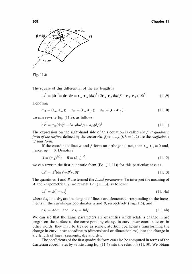
The square of this differential of the arc length is

ds2 ¼ drj j2¼ dr � dr ¼ r; �r; dð Þ2þ2r; �r; ddþ r; �r; dð Þ2: ð11:9ÞDenoting

a11 ¼ ðr; �r; Þ; a12 ¼ ðr; �r; Þ; a22 ¼ ðr; �r; Þ; ð11:10Þwe can rewrite Eq. (11.9), as follows:

ds2 ¼ a11ðdÞ2 þ 2a12ddþ a22ðdÞ2: ð11:11ÞThe expression on the right-hand side of this equation is called the first quadraticform of the surface defined by the vector rð; Þ and aik ði; k ¼ 1; 2Þ are the coefficientsof that form.

If the coordinate lines and form an orthogonal net, then r; �r;¼ 0 and,hence, a12 ¼ 0. Denoting

A ¼ ða11Þ1=2; B ¼ ðb11Þ1=2; ð11:12Þwe can rewrite the first quadratic form (Eq. (11.11)) for this particular case as

ds2 ¼ A2 dð Þ2þB2 dð Þ2: ð11:13ÞThe quantities A and B are termed the Lame parameters. To interpret the meaning ofA and B geometrically, we rewrite Eq. (11.13), as follows:

ds2 ¼ ds21 þ ds22; ð11:14aÞwhere ds1 and ds2 are the lengths of linear arc elements corresponding to the incre-ments in the curvilinear coordinates and , respectively (Fig.11.6), and

ds1 ¼ Ad and ds2 ¼ Bd: ð11:14bÞWe can see that the Lame parameters are quantities which relate a change in arclength on the surface to the corresponding change in curvilinear coordinate or, inother words, they may be treated as some distortion coefficients transforming thechange in curvilinear coordinates (dimensional or dimensionless) into the change inarc length of linear segments, ds1 and ds2.

The coefficients of the first quadratic form can also be computed in terms of theCartesian coordinates by substituting Eq. (11.4) into the relations (11.10). We obtain

308 Chapter 11

Fig. 11.6

a11 ¼ X;ð Þ2þ Y;ð Þ2þ Z;ð Þ2; a12 ¼ X; X;þY; Y;þZ; Z; ;

a22 ¼ X;� �2þ Y;

� �2þ Z;� �2

:ð11:15Þ

The first quadratic form generally pertains to the measurement of distancesalong an arc between two points on a surface, to areas on the surface, and to anglesbetween any two curves passing through a point (i.e., the angle between the tangentsto these curves), etc. Thus, the first quadratic form defines the intrinsic geometry ofthe surface. However, it does not involve the specific shape of the surface. Forinstance, this form cannot be a measure of curvature of curves lying on a surfaceor if we change a curvature of the surface (say, by its bending) without its stretchingor contracting, the first quadratic form remains unchanged. So, the representation ofthe surface by the Lame parameters only is not sufficient and the first quadratic formmust be complemented with the second quadratic form to describe uniquely theintrinsic and extrinsic geometries of a surface.

The second quadratic form describes a shape of the surface, given by Eq. (11.1).This problem is associated with finding a curvature of the surface at a point. Thenotion of curvature of the surface is an extension of the notion of curvature of aplane curve, discussed in Sec. 11.2.

Consider a normal section which traces a plane curve with a unit inwardnormal e3 directed toward the center of curvature of the curve. The curvature ofthat normal section, called the normal curvature and denoted by �n, is of the follow-ing form (a detailed derivation of this expression is given in Appendix C.2):

�n ¼ II

I¼ b11 dð Þ2þ2b12ddþ b22 dð Þ2

a11 dð Þ2þ2a12ddþ a22 dð Þ2 ; ð11:16Þ

where

b11 ¼ e3 �@2r

@2; b12 ¼ e3 �

@2r

@@; b22 ¼ e3 �

@2r

@2; ð11:17Þ

and the coefficients aik ði; k ¼ 1; 2Þ are given by Eqs (11.10). It can be seen thatexpression I in the denominator of Eq. (11.16) represents the first quadratic formof the surface for any coordinate curves that are not orthogonal (see Eq. (11.11)).

Expression II is called the second quadratic form of surfaces:

II ¼ b11 dð Þ2þ2b12ddþ b22 dð Þ2; ð11:18Þand the quantities b11; b12; and b22 are referred to as the coefficients of the secondquadratic form of surfaces. The coefficients b11 and b22 characterize the normalcurvature of lines ¼ const: and ¼ const, respectively, whereas the coefficientb12 describes the twisting of the surface. Thus, the second quadratic form definescompletely a curved shape of a surface in the neighborhood of a point of interest.

The coefficients of the second quadratic form bik ði; k ¼ 1; 2Þ were given interms of the curvilinear coordinates and . They can also be expressed in termsof the Cartesian coordinates X;Y; and Z (see Eqs (C.11) in the Appendix C.2).

As mentioned previously, the simultaneous use of the first and second quad-ratic forms define completely and uniquely a surface with the accuracy of its locationin the space. This means that two surfaces having the same first and second quadratic


forms coincide in their configuration and can be different only by their location inthe space.

11.4 PRINCIPAL CURVATURES

As mentioned in Sec. 11.2, through every point M of a smooth surface the normalcurvature, �n, in general varies with the direction through the point. However, thereare two orthogonal directions on which �n is extremal (�max ¼ �1 and �min ¼ �2) andthese are what have been named in Sec. 11.2 the principal directions. It is seen fromEq. (11.16) that the normal curvature at point M of a surface depends on a directionof the section, � ¼ d=d. Determine the values of � that correspond to the extremalvalues of �n. For this purpose, transform Eq. (11.16), by inserting the parameter �, tothe form

�nð�Þ ¼b11 þ 2b12�þ b22�

2

a11 þ 2a12�þ a22�2: ð11:19Þ

The desired values of � are evaluated from the condition d�n=d� ¼ 0. The latterresults in the following equation:

ðb12a22 � b22a12Þ�2 þ ðb11a22 � b22a11Þ�þ ðb11a12 � b12a11Þ ¼ 0:

This equation defines the two roots, �1 and �2, corresponding to the two principaldirections, i.e.,

�1;2 ¼�ðb11a22�b22a11Þ�

ffiffiffiffiffiffiffiffiffiffiffiffiffiffiffiffiffiffiffiffiffiffiffiffiffiffiffiffiffiffiffiffiffiffiffiffiffiffiffiffiffiffiffiffiffiffiffiffiffiffiffiffiffiffiffiffiffiffiffiffiffiffiffiffiffiffiffiffiffiffiffiffiffiffiffiffiffiffiffiffiffiffiffiffiffiffiffiffiffiffiffiffiffiffiffiffiffiffiffiffiffiffiffiffiffiffiðb11a22� a11b22Þ2�4ðb12a22�b22a12Þðb11a12�b12a11Þ

q2ðb12a22 � b22a12Þ

:

ð11:20ÞOne of the roots, �1, being substituted into Eq. (11.19), corresponds to the maximumvalue of the normal curvature, �1, while the second one, �2, corresponds to theminimum value, �2.

We have postulated in Sec. 11.2 that the curvilinear coordinate lines and are to be the principal directions. It can be shown (see Appendix C.2) that theprincipal directions are mutually orthogonal. From the orthogonality condition(C.13) or (C.14) (see Appendix C.2), and from Eqs (11.10), we obtain that

a12 ¼ b12 ¼ 0 ð11:21Þif the curvilinear coordinate lines and are chosen to coincide with the principaldirections. The values of the principal curvature can be immediately determinedfrom Eq. (11.16) by setting a12 ¼ b12 ¼ 0 and then letting d ¼ 0 and d ¼ 0, inturn, to give

�1 ¼1

R1

¼ b11a11

; �2 ¼1

R2

¼ b22a22

: ð11:22Þ

The expression of the second quadratic form, Eq. (11.18), when the principal direc-tions (or the lines of curvature) are used as the curvilinear coordinate curves, sim-plifies to the form

II ¼ b11ðdÞ2 þ b22ðdÞ2: ð11:23Þ

310 Chapter 11

11.5 UNIT VECTORS

As mentioned previously, all vector quantities in the theory of shells, which arefunctions of points on the middle surface, will be given in terms of their projectionson the directions of the tangents to some reference axes (the coordinate lines and ,and normal to the surface at a point of interest). Since these reference axes changetheir directions when passing from one point of the surface to another one, it isnecessary to investigate the differentiation of these vector quantities with respect to and .

A triad of the unit orthogonal vectors composed at a point on the middlesurface of tangent vectors e1 and e2 to the coordinate lines and , and an inwardnormal vector e3 directed toward the center of curvature of the shell, represent alocal vectorial basis to which the displacements, stress resultants, and stress couplesare assigned. This basis defines a right-hand system, as shown in Fig. 11.7. Takinginto account the expressions (11.5), (11.10), and (11.12), we can introduce the unitvectors as follows:

e1 ¼r;r; ¼ r;

A; e2 ¼

r;

r; ¼ r;

B; e3 ¼ e1 e2 ¼

1

ABr; r;� � ð11:24Þ

Any vector T may be represented in terms of the introduced orthogonal unit vectors,as follows:

T ¼ T1e1 þ T2e2 þ T3e3;

where T1;T2; and T3 are components of the vector in the coordinate basis (Eq.(11.24)). A partial derivative of the above vector T with respect to any coordinatemay be represented as

@T

@¼ @T1

@e1 þ

@T2

@e2 þ

@T3

@e3 þ T1

@e1@

þ T2

@e2@

þ T3

@e3@: ð11:25Þ

The laws of differentiating the vectors, represented by Eq. (11.25), are reduced to thefollowing form (a detailed derivation of these expressions is given in Appendix C.3):

@e1@

¼ � 1

B

@A

@e2 þ

A

R1

e3;@e1@

¼ 1

A

@B

@e2;

@e2@

¼ 1

B

@A

@e1;

@e2@

¼ � 1

A

@B

@e1 þ

B

R2

e3;

@e3@

¼ � A

R1

e1;@e3@

¼ � B

R2

e2:

ð11:26Þ


Fig. 11.7

314

Fig. 11.9

(b) Paraboloid of revolution (Fig. 11.9d)

The equation of the meridional curve is given by

r2 � 2pZ ¼ 0 or r2 ¼ a2

bZ; ðdÞ

where p is a parameter of the parabola. Using the technique considered above for theellipsoid of revolution, we present below the final expressions for the principal radiiof curvature for the paraboloid, dropping the intermediate mathematics,

R1 ¼a2

2b

1

cos2 ’� �3=2 ; R2 ¼

a2

2b

1

cos ’; ð11:47Þ

where b is the height of the paraboloid and a is one-half the length of the paraboloidbase.

(c) Sphere (Fig. 11.9e)

Consider a spherical shell of radius a. It can be easily shown that the principal radiusof the meridian is equal to the radius of the generating circle a. Indeed, the equationof the meridian is

Z2 þ r2 ¼ a2:

With r;Z ¼ �Z=r and r;ZZ ¼ � 1=rð Þ 1þ Z2=r2� �

, we find from Eq. (11.45) that theprincipal radii of the sphere are

R1 ¼1þ Z=rð Þ2� �3=21=rð Þ 1þ Z2=r2

� � ¼ ffiffiffiffiffiffiffiffiffiffiffiffiffiffiffiffiZ2 þ r2

q¼ a and R2 ¼ r 1þ z2

r2

!1=2

¼ffiffiffiffiffiffiffiffiffiffiffiffiffiffiffiffir2 þ Z2

p¼ a:

Thus, for a spherical shell, both the principal radii of curvature are equal to theradius of the generating circle a.

(d) Hyperboloid of revolution (Fig. 11.9f)

The equation of the generating curve (hyperbola) is

r2

a2� Z2

b2¼ 1; ðeÞ

where a is one-half the length of the reference section of the hyperboloid and b issome characteristic dimension of the hyperboloid. The latter may be evaluated bysubstituting the base coordinates s;Sð Þ and the top coordinates ðt;TÞ into the equa-tion of the hyperbola, i.e.,

b ¼ aTffiffiffiffiffiffiffiffiffiffiffiffiffiffit2 � a2

p ¼ aSffiffiffiffiffiffiffiffiffiffiffiffiffiffis2 � a2

p :

For the radii of curvature we have to use the same formulas as for the ellipsoid (i.e.,Eqs (11.46)), replacing b2 by �b2. Thus, we obtain

R1 ¼ � a2b2

a2 sin2 ’� b2 cos2 ’� �3=2 ; R2 ¼

a2

a2 sin2 ’� b2 cos2 ’� �1=2 : ð11:48Þ

320 Chapter 11

where x is the distance measured from some reference profile to the point of interestand � is the angle between the normal to the shell at a point and a reference normalat a chosen origin.

Consider an element of the shell, bounded by sections x; xþ dx and �; � þ d�(Fig. 11.13). The first quadratic form of the surface will be here, as follows:

ds2 ¼ dx2 þ R22d�

2; ð11:51Þwhere R2 is the second principal radius of curvature, while the first principal radius isinfinite, i.e., R1 ¼ 1: Comparing the above with the relation (11.12), one can obtainthe Lame parameters for the cylindrical shell of a general shape, as follows:

A ¼ 1; B ¼ R2: ð11:52ÞFor a circular cylindrical shell, R2 ¼ const ¼ R, where R is the radius of the circularcylinder. So, the Lame parameters for the circular cylindrical shell are

A ¼ 1; B ¼ R ¼ const: ð11:53Þ

11.8.3 Conical shells

In a conical shell, the meridional angle ’ is a constant and can no longer serve as acoordinate of the meridian. The location of a point on the middle surface will bedefined by the radius vector r taken from the top of the cone (point O in Fig. 11.14)along its generator, and angle � formed by a meridional plane passing through thatpoint with some reference meridional plane. Let the length of the vector r be s andthe slope of the generator to the cone base be . The projections of r on the globalcoordinate axes, X;Y; and Z (see Fig. 11.14) are

X ¼ s cos cos �; Y ¼ s cos sin �; Z ¼ s sin : ð11:54ÞThe vector r can be resolved along the unit vectors i; j; and k, as follows:

r ¼ s i cos cos � þ j cos sin � þ k sin ð Þ: ð11:55Þ

322 Chapter 11

Fig. 11.14

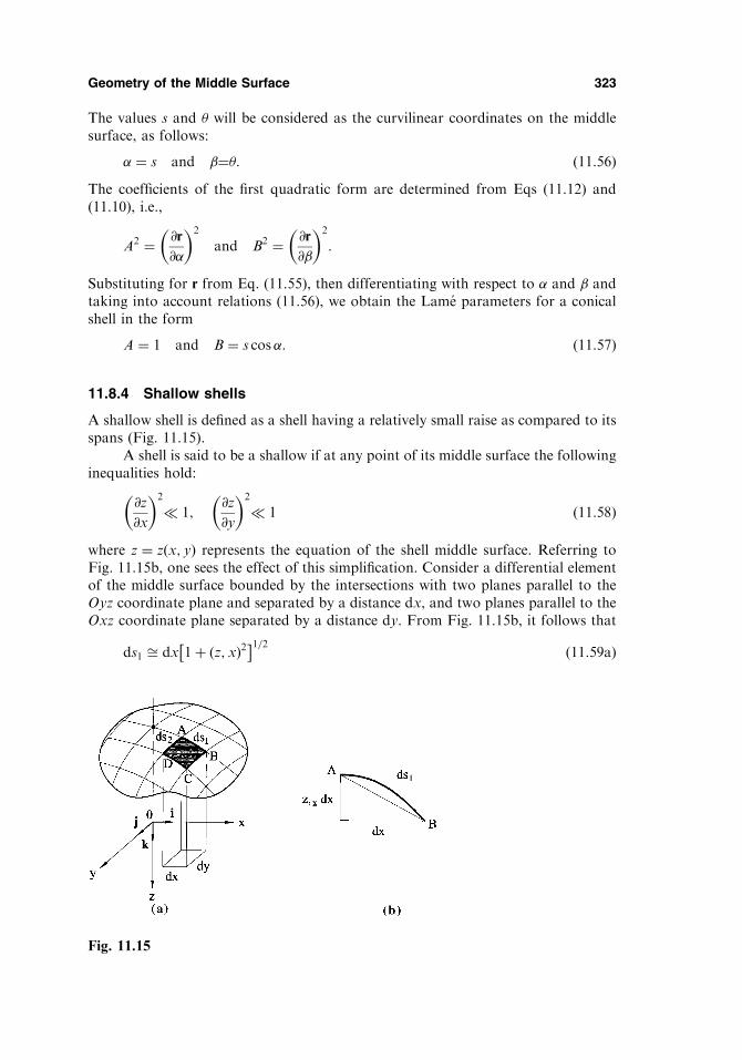
The values s and � will be considered as the curvilinear coordinates on the middlesurface, as follows:

¼ s and ¼�: ð11:56ÞThe coefficients of the first quadratic form are determined from Eqs (11.12) and(11.10), i.e.,

A2 ¼ @r

@

� �2

and B2 ¼ @r

@

� �2

:

Substituting for r from Eq. (11.55), then differentiating with respect to and andtaking into account relations (11.56), we obtain the Lame parameters for a conicalshell in the form

A ¼ 1 and B ¼ s cos: ð11:57Þ

11.8.4 Shallow shells

A shallow shell is defined as a shell having a relatively small raise as compared to itsspans (Fig. 11.15).

A shell is said to be a shallow if at any point of its middle surface the followinginequalities hold:

@z

@x

� �2

� 1;@z

@y

� �2

� 1 ð11:58Þ

where z ¼ z x; yð Þ represents the equation of the shell middle surface. Referring toFig. 11.15b, one sees the effect of this simplification. Consider a differential elementof the middle surface bounded by the intersections with two planes parallel to theOyz coordinate plane and separated by a distance dx, and two planes parallel to theOxz coordinate plane separated by a distance dy. From Fig. 11.15b, it follows that

ds1 ffi dx 1þ z; xð Þ2� �1=2 ð11:59aÞ


Fig. 11.15

Similarly, we can write

ds2 ffi dy 1þ z; yð Þ2� �1=2: ð11:59bÞ

These expressions, due to the geometric simplification (Eq. (11.58)), may be writtensimply as

ds2 � dy and ds1 � dx: ð11:60ÞPractically, the above imply that the curvilinear coordinates and may be selectedas the Cartesian coordinates x and y with the following Lame parameters:

A ¼ B ¼ 1: ð11:61Þ

PROBLEMS

11.1 Verify Eqs (11.28) and (11.29).

11.2 Draw sketches of the following meridians and calculate the principal curvatures �1 and�2 in each case: (a) Z ¼ Ar2; and (b) ðr=aÞ2 � ðz=bÞ2 ¼ 1.

11.3 Explain the difference between the first and second quadratic forms from the geometric

point of view.

11.4 Roof shell structures often have a shape of surfaces of translation (see Sec. 11.7.1(b)).

The equation of such a surface can be assigned as Z ¼ ’ðXÞ þ ðYÞ. Assuming that a

location of a point on this surface is given by the Cartesian coordinates ¼ x and

¼ y, determine the coefficients of the first quadratic form for the nonshallow shell of

translation.

11.5 Verify Eqs. (11.45) and (11.47).

11.6 Verify that the Gauss–Codazzi relations are satisfied for a shell of revolution with the

parameter A given by equation A ¼ ½1þ ðr;ZÞ2�1=2.11.7 Verify Eqs (11.48).

11.8 Calculate the Lame parameters for a conical shell in terms of the coordinates Z and �(see Fig. 11.15), i.e., for ¼ Z and ¼ �:

11.9 Prove that surfaces possessing the same Lame parameters will have the same Gaussian

curvature.

REFERENCES

1. Louis, A., Differential Geometry, Harper and Row, New York, 1967.

2. Stoker, J.J., Differential Geometry, Wiley-Interscience, New York, 1969.

3. Kreyszig, E., Differential Geometry, University of Toronto, Toronto, 1959.

4. Kelkar, V.S. and Sewell, R.T., Analysis & Design of Shell Structures, Prentice-Hall,

Englewood Cliffs, New Jersey, 1987.

5. Novozhilov, V.V., Thin Shell Theory, P. Noordholf, Groningen, The Netherlands, 1964.

324 Chapter 11

shell may be simplified to the form (neglecting here the value of z=Ri in comparisonwith unity)

"z1 ¼ "1 þ z�1; ð12:22aÞ"z2 ¼ "2 þ z�2; ð12:22bÞ�z12 ¼ �12 þ 2z�12: ð12:22cÞ

In so doing, it cannot be stated that the linear in z Eqs (12.22) are less accurate thanEqs (12.10) and (12.21).

The relations (12.22) are of primary importance in the theory of shells. Theyexpress the normal and shear strain components at any point across the shell thick-nesses as a linear combination of the following two terms:

(a) the in-plane strain components on the middle surface that are expressedin terms of the middle surface displacements by Eqs (12.3)–(12.5);

(b) the changes in curvature and twist that are also given in terms of themiddle surface displacements by Eqs (12.12), (12.13), and (12.19).

Therefore, as mentioned previously, the relations (12.22) enable one to reduce the 3Dproblem of the shell straining to the 2D problem of the deformation of the shellmiddle surface. The relationships between the in-plane strains, changes in curvature,and twist on the one hand, and the displacements of the middle surface on the other,are called the generalized strain–displacement or kinematic equations. They establishthe conditions of compatibility of the strains and displacements, suitably specializedfor the shell theory under consideration. Let us summarize these equations, asfollows:

"1 ¼1

A

@u

@þ 1

AB

@A

@v� w

R1

;

"2 ¼1

B

@v

@þ 1

AB

@B

@u� w

R2

;

�12 ¼B

A

@

@

v

B

� �þ A

B

@

@

u

A

� �; ð12:23Þ

�1 ¼ � 1

A

@

@

u

R1

þ 1

A

@w

@

� �þ 1

AB

@A

@

v

R2

þ 1

B

@w

@

� �� ;

�2 ¼ � 1

B

@

@

v

R2

þ 1

B

@w

@

� �þ 1

AB

@B

@

u

R1

þ 1

A

@w

@

� �� ;

�12 ¼ � 1

AB� 1

A

@A

@

@w

@� 1

B

@B

@

@w

@þ @2w

@@

!þ 1

R1

A

B

@

@

u

A

� �þ 1

R2

B

A

@

@

v

B

� �" #;

ð12:24Þ"3 ¼ �13 ¼ �23 ¼ 0: ð12:25Þ

It follows from the above equations that a deformation of the shell middle surface iscompletely defined by the six strain parameters, "1; "2; �12;�1; �2; and �12 that are

General Theory of Shells 331

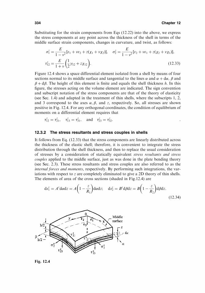
Substituting for the strain components from Eqs (12.22) into the above, we expressthe stress components at any point across the thickness of the shell in terms of themiddle surface strain components, changes in curvature, and twist, as follows:

�z1 ¼E

1� �2 "1 þ �"2 þ z �1 þ ��2ð Þ½ �; �z2 ¼E

1� �2 "2 þ �"1 þ z �2 þ ��1ð Þ½ �;

�z12 ¼E

1þ �1

2�12 þ z�12

� �: ð12:33Þ

Figure 12.4 shows a space differential element isolated from a shell by means of foursections normal to its middle surface and tangential to the lines and þ d; andþ d. The height of this element is finite and equals the shell thickness h. In thisfigure, the stresses acting on the volume element are indicated. The sign conventionand subscript notation of the stress components are that of the theory of elasticity(see Sec. 1.4) and adapted in the treatment of thin shells, where the subscripts 1, 2,and 3 correspond to the axes ; ; and z, respectively. So, all stresses are shownpositive in Fig. 12.4. For any orthogonal coordinates, the condition of equilibrium ofmoments on a differential element requires that

�z12 ¼ �z21; �z13 ¼ �z31; and �z23 ¼ �z32: :

12.3.2 The stress resultants and stress couples in shells

It follows from Eq. (12.33) that the stress components are linearly distributed acrossthe thickness of the elastic shell; therefore, it is convenient to integrate the stressdistribution through the shell thickness, and then to replace the usual considerationof stresses by a consideration of statically equivalent stress resultants and stresscouples applied to the middle surface, just as was done in the plate bending theory(see Sec. 2.3). These stress resultants and stress couples are also referred to as theinternal forces and moments, respectively. By performing such integrations, the var-iations with respect to z are completely eliminated to give a 2D theory of thin shells.The elements of area of the cross sections (shaded in Fig.12.4) are

dsz1 ¼ Azddz ¼ A 1� z

R1

� �ddz; dsz2 ¼ Bzddz ¼ B 1� z

R2

� �ddz:

ð12:34Þ

334 Chapter 12

Fig. 12.4

@

@N1Bð Þ þ @

@N21Að Þ þN12

@A

@�N2

@B

@�Q1

AB

R1

þ p1AB ¼ 0;

@

@N2Að Þ þ @

@N12Bð Þ þN21

@B

@�N1

@A

@�Q2

AB

R2

þ p2AB ¼ 0;

@

@Q1Bð Þ þ @

@Q2Að Þ þN1

AB

R1

þN2

AB

R2

þ p3AB ¼ 0; ð12:41Þ

@

@BM12ð Þ þ @

@AM2ð Þ �M1

@A

@þM21

@B

@�Q2AB ¼ 0;

@

@AM21ð Þ þ @

@BM1ð Þ �M2

@B

@þM12

@A

@�Q1AB ¼ 0;

N12 �N21 �M12

R1

þM21

R2

¼ 0: ð12:42Þ

The detailed derivations of Eqs (12.41) and (12.42) are given in Appendix E. Theabove equations represent a set of the differential equations of static equilibrium of ashell element of the general theory of thin elastic shells.

It can be easily shown that the third Eq. (12.42) is identically satisfied. Toprove that, one needs to substitute for N12;N21; and M12;M21 from Eqs (12.35) and(12.36) into the third Eq. (12.42). We obtain the following:

ðh=2�h=2

�z12 1� z

R2

� �dz�

ðh=2�h=2

�z21 1� z

R1

� �dz�

ðh=2�h=2

�z12z

R1

1� z

R2

� �dz

¼ðh=2�h=2

�z21z

R2

1� z

R1

� �dz ¼

ðh=2�h=2

1� z

R2

� �1� z

R1

� ��z12 � �z21ð Þdz � 0

because �z12 ¼ �z21:

Hence, the system of three equations (Eqs (12.42)) can be reduced to twoequations and the third equation may be disregarded, although we may mention itfrom time to time.

Novozhilov [1] suggested that we reduce the number of unknowns in the aboveequations by setting

M12 ¼ M21 ¼ H; S ¼ N12 þH

R2

¼ N21 þH

R1

: ð12:43Þ

It can be shown that the substitution of these expressions for N12;N21;M12; and M21

from Eqs (12.43) into the third Eq. (12.42) results in the identity, 0 � 0. Thus, takinginto account relations (12.43), the equilibrium equations (12.41) and (12.42) arefinally reduced to the system of five partial differential equations for eight unknownstress resultants and couples: i.e., N1;N2;S;M1;M2;H;Q1; and Q2.

Determining the transverse shear forces Q1 and Q2 from the first and secondEqs (12.42) and substituting them into Eqs (12.41) with the replacement N12 ¼ S �H=R2 and N21 ¼ S �H=R1, we arrive at three equations of equilibrium in the fol-lowing form:

338 Chapter 12

In the first-order approximation shell theory, the constitutive relations for N12

and N21 are usually simplified to the form

N12 ¼ N21 ¼ S ¼ Eh

2 1þ �ð Þ �12: ð12:48Þ

In this form, the constitutive equations (12.45), (12.46), and (12.48) remind us of thecorresponding stress resultants–strains and stress couple–curvatures relations dis-cussed previously in the plate bending theory (Sec. 2.3). The difference betweenthe two constitutive equations is that the strain–displacement relations in the generalshell theory have a more complex form than in the plate theory. However, as men-tioned in Ref. [1], although the error introduced by the simplified relation (12.48)does not exceed the corresponding errors of the general assumptions adopted in theshell theory, the application of the above equation brings some contradictions. Butthese contradictions do not practically influence the accuracy of the calculations ofthe stress and displacement components.

12.4 STRAIN ENERGY OF SHELLS

The strain energy of the shell can be determined by means of Kirchhoff’s assump-tions discussed previously, i.e., the transverse normal, �3, and shear, �13 and �23,stress components are neglected. Therefore, the strain energy density (strain energyper unit volume) uu is given by [1]:

uu ¼ 1

2Eð�z1Þ2 þ ð�z2Þ2 � 2��z1�

z2

� �þ 1

2Gð�z12Þ2

or

uu ¼ E

2 1� �2� � "z1ð Þ2þ "z2ð Þ2þ2�"z1"z2

h iþ G

2�z12ð Þ2: ð12:49aÞ

Since G ¼ E=2 1þ �ð Þ, the last equation may be rewritten as

uu ¼ E

2 1� �2� � "z1 þ "z2ð Þ2þ2 1� �ð Þ 1

4�z12ð Þ2� "z1"

z2

� �� : ð12:49bÞ

Substituting for "z1; "z2; and �

z12 from Eqs (12.22) into the above:

uu ¼ E

2 ð1� �2 Þ "1 þ "2 þ zð�1 þ �2½ Þ�2

þ 2ð1� �Þ 1

4ð�12 þ 2�12zÞ2 � ð"1 þ �1zÞð"2 þ �2zÞ

� ��:

ð12:50Þ

To calculate the total strain energy of the shell, it is necessary to multiply the straindensity uu by an elementary volume of the layer of the shell, as follows:

dV ¼ AzBzdddz ¼ 1� z

R1

� �1� z

R2

� �ABdddz;

and to integrate over the shell thickness (�h=2 � z � h=2) and over the area of itsmiddle surface.

340 Chapter 12

direction of the closed coordinate the conditions of periodicity must be formulatedas the boundary conditions. Along the other, the open coordinate, it is necessary toset up the boundary conditions, which are to be satisfied in solving the governingdifferential equations of the general shell theory.

3. A shell is open with regard to both coordinate lines and . In this case, it isrequired to set up certain boundary conditions in the directions of both principaldirections. Proceeding now to this general case, we confine ourselves to the simplestcase where the boundaries coincide with the lines of principal curvature of the middlesurface (the - and - coordinate lines), since this case is encountered most frequentlyin practice.

Let, for example, the line ¼ be a boundary of the shell. The stresses actingon the boundary can be reduced to the three internal forces N2;N21; and Q2 and twomomentsM2 andM21. The deformations on the same boundary are characterized bythe three displacement components u; v; and w and two slopes #1 and #2. Thus, atfirst glance, five boundary conditions must be prescribed on the edge line ¼ .However, this is not true: due to the Kirchhoff kinematic hypothesis (the firstKirchhoff assumption), not all the above-mentioned quantities are independent.The slope of the normal to the shell boundary, #2, is connected with the displace-ments w and v on this boundary by the condition of the preservation of the normal.Therefore, the number of independent displacements (and hence, the correspondinggeneralized forces) equals four, and only the four boundary conditions can beassigned on each edge of the shell. By the way, as follows from the above, such anumber of independent boundary conditions corresponds to the eighth order of thegoverning differential equations of the general linear theory of thin shells.

Thus, the five forces and moments assigned for the static boundary conditionson the shell boundary (i.e., the boundary conditions expressed in terms of the inter-nal forces and moments) can be reduced to four quantities in accordance withKirchhoff’s postulates. This can be carried out in a similar manner to that done inthe plate theory (Sec. 2.5): namely, the three boundary quantities, N2;N21; and M21,may be replaced with the two boundary quantities with an acceptable accuracy.

Figure 12.6 shows two adjacent differential segments of the boundary ¼

of the middle surface, each of length ds1, near some point m1. The boundary curvemm1m2 may be approximated by a polygon formed by two small segments of equallength. The length of each such segment with a high order of accuracy may be setequal to the length of the arc spanning, i.e., mm1 ¼ m1m2 � ds1. Let points n1 and n2be halfway between the points m and m1;m1 and m2, respectively. It is evident thatn1n2 � ds1. Let M21ds1 and

M21 þ@M21

@s1ds1

� �ds1

be the resultants of the twisting moments distributed over segments mm1 and m1m2,respectively. These act at the midpoints n1 and n2. Further, we replace each of theabove resultant couples by a pair of equal and opposite forces with the moment armsds1 and applied at end points of the corresponding segments. So, at end points mand m1 the forces M21ds1ð Þ=ds1 ¼ M21, acting normal to the chord mm1, are applied.Similarly, the forces M21 þ @M21=@s1ð Þds1, acting normal to the chord m1m2, will beapplied at end points m1 and m2. Thus at each point of the corners of the polygon,

342 Chapter 12

two concentrated forces from twisting moments distributed over the adjacent seg-ments are applied, as shown in Fig. 12.6b for corner point m1.

Projecting both these forces, acting at a point m1, on the direction of thenormal to the middle surface (the direction of the transverse shear force Q2) andon the direction of the tangent to the middle surface (the direction of the in-planeshear force N21), we obtain:

(a) in the first case

þM21

@M21

@s1ds1 �M21 ¼

@M21

@s1ds1; ðaÞ

(b) in the second case

� 2M21 þ@M21

@s1ds1

� �’; ðbÞ

where 2’ is the angle between the normals to the middle surface at points n1 and n2,i.e., 2’ ¼ ds1=R1. Substituting this value for ’ into the expression (b) and retainingonly the first-order quantities, one finds �ðM21=R1Þds1. Thus, along the shell edge ¼ , the twisting moment can be replaced by the distributed normal (transverse)shear forces @M21=@s1 and distributed tangential (in-plane) shear forces �M21=R1.

As mentioned previously (see Sec. 2.5), the replacement of the twisting momentby statically equivalent forces results in a certain redistribution of the stresses overthe thickness of the shell along its boundaries. By the St.Venant principle, the effectof this approximation cannot be significant; it can only be noticeable within theimmediate neighborhood of the boundaries (at distances of the order of the shellthickness).

It follows from the above that the boundary conditions on the edge ¼ canbe formulated in terms of the following four quantities:


Fig. 12.6

(1) The strain–displacement relations

Six strain–displacement equations are summarized for the general linear shell theoryby Eqs (12.23) and (12.24). They involve six components of strain, "1; "2; �12; �1; �2;and �12, which are given explicitly in terms of the three displacement componentsu; v; and w. Note that the six strain components must satisfy the equations ofcompatibility (Eqs (12.27)). The latter equations are used only for solving the shellproblems in forces–strain components. If the problem under consideration is solvedin terms of the displacement components, then these conditions are satisfiedautomatically.

(2) The constitutive equations

The eight equations are summarized in the general case by Eqs (12.45) and (12.46).They express the eight stress resultants and stress couples, N1; N2; N12; N21;M1;M2;M21; and M12, as explicit functions of the six strain components, "1; "2; �12; �1; �2;and �12. The number of these constitutive equations can be reduced for a practicalstress analysis of shells to six by accepting the assumption (12.43).

(3) Equations of equilibrium

Five equations of equilibrium must be satisfied. They are given by Eqs (12.41) and(12.42). These five equations involve the 10 stress resultants and couple resultants,N1; N2;N12; N21;M1; M2; M12; M21; Q1; and Q2. The number of the these forcesand moments can be reduced to eight by using Eqs (12.43).

(4) Boundary conditions

Boundary conditions relate the stress resultants and stress couples or displacementcomponents specified on the shell boundaries to prescribed boundary quantities (in aparticular case, the latter may be equal to zero). These boundary conditions aresummarized by Eqs (12.56)–(12.59).

Thus, in general, there are 19 equations relating 19 unknowns, u; v; w; "1; "2;�12; �1; �12; N1; N2; N12; N21; M1 ;M2; M12; M21;Q1, and Q2. For a simplifiedgeneral linear theory of shells, one can take N12 ¼ N21 and M12 ¼ M21, therebyreducing the number of equations and unknowns to 17.

As for the theory of elasticity, shell problems may be solved either in terms ofdisplacements or in terms of the internal forces and moments. According to the firsttechnique, the internal forces and moments are replaced in the equilibrium equations(12.41) and (12.42) by the displacement components u; v; and w, using the constitu-tive and strain–displacement relations (12.45), (12.46) and (12.23), (12.24), respec-tively. As a result, the eight-order system of the three governing partial differentialequations for displacements is obtained. The second technique consists of simulta-neous treatment of equations of equilibrium (12.41) and (12.42) or (12.44) andcompatibility relations (12.27). In so doing, the eight-order system of six governingdifferential equations for N1; N2; S; M1; M2; and H will be obtained.


12.7 TYPES OF STATE OF STRESS FOR THIN SHELLS

All equations mentioned in Sec. 12.6 are linear for both techniques, which, of course,greatly simplifies their study and solution. However, shell problems associated withcalculations of the stress and strain components remain very difficult. As a rule, thegoverning, eight-order partial differential equations of the general shell theory havevariable coefficients. Mathematical difficulties associated with integration of such atype of differential equations are evident. Even for the simplest circular cylindricalshells for which the governing equations have constant coefficients, cumbersomecomputations remain involved and,by far, not all problems of practical interestfor such shells have been solved. Consequently, attempts of scientists and engineersengaged in the practical stress analysis of shell structures were directed towards thesearch for possibilities of simplifying the above governing differential equations ofthe general shell theory and shell problems themselves. Several approximate methodsand the corresponding shell models based upon some additional assumptions andupon simplified governing equations are considered in Chapter 17.

Previously, in presenting the general linear shell theory, it was assumed that theflexural stresses are values of the same order as the stresses caused by in-plane(membrane) stresses. If one of the above-mentioned types of stresses is negligiblein comparison with another one, then it is possible to introduce considerable sim-plifications in the general linear shell theory. Consider some possible types of state ofstress for thin shells.

1. If the flexural stresses are negligible compared with the membrane stressesthen such a type of state of stress is called a membrane or momentless state of stress.The governing equations of the membrane theory can be obtained directly from theequations of the general shell theory by neglecting the effect of the bending andtwisting moments, as well as the transverse shear forces, on the state of stress andstrain of thin shells. In some cases, the membrane theory describes the state of stressand strain with reasonable accuracy, since the bending and twisting moments are ofnegligible magnitudes: for example, hollow spherical shells subjected to inside andoutside uniform pressure are in the pure membrane state of stress.

2. If, to the contrary, the membrane stresses are negligible in comparison withthe flexural stresses, then such a type of state of stress is referred to as a pure flexuralor moment state of stress. Note that the definitions of the ‘‘membrane’’ and ‘‘pureflexural’’ states of stress are not quite correct because the membrane state of stressadmits an existence of small flexural stresses and, in turn, small membrane stressesmay occur in a pure flexural state of stress. It was mentioned previously that shells,due to their small thickness, possess a relatively small flexural stiffness and, there-fore, they are poorly adapted to resisting in bending. Even relatively small bendingmoments may cause considerable flexural stresses and displacements in shells.Therefore, a pure flexural type of the state of stress is dangerous and technicallydisadvantageous for thin shells. It should be avoided by introducing some intermedi-ate reinforcements, by selecting the corresponding shape of the shell, by choosing thetype of supports, etc. Conversely, the membrane state of stress, at which the shell isuniformly stressed across its thickness, is technically the most advantageous. So,engineers designing a shell should aim at such a state of stress.

3. If the flexural and membrane stresses are of the same order, then such astate of stress is called a mixed state of stress, or edge effect. The term ‘‘edge effect’’ is

346 Chapter 12

stability only when the compressive forces exceed a certain critical value. For abso-lutely flexible shells, since they do not possess a resistance to bending, only themembrane state of stress is possible, while for shells with finite stiffness such astate of stress is only one of the possible stress conditions. In this chapter we consideronly shells with a finite flexural stiffness.

13.2 THE FUNDAMENTAL EQUATIONS OF THE MEMBRANETHEORY OF THIN SHELLS

The governing equations of the membrane theory can be obtained directly from theequations of the general theory of thin shells derived in Chapter 12. For this purpose,it is assumed that, in view of the smallness of the changes of curvature and twist, themoment terms in the equations of equilibrium for a shell element are unimportant,although in principle the shell may resist the external loads in bending. Note thatneglecting the moments leads to neglecting the normal shear forces. Thus, for themembrane theory of thin shells, we can assume that

M1 ¼ M2 ¼ H ¼ Q1 ¼ Q2 ¼ 0: ð13:3ÞIntroducing Eq. (13.3) into Eqs (12.44) and taking into account Eq. (12.43), onearrives at the following system of differential equations:

@

@N1Bð Þ þ 1

A

@

@A2S� ��N2

@B

@þ ABp1 ¼ 0;

@

@N2Að Þ þ 1

B

@

@B2S� ��N1

@A

@þ ABp2 ¼ 0;

N1

1

R1

þN2

1

R2

þ p3 ¼ 0;

ð13:4Þ

where N12 ¼ N21 ¼ S (since H ¼ 0Þ.In this system, the number of unknowns is equal to the number of equations, so

the problem of the membrane theory of shells is statically determinate (that is truefor the equilibrium of an infinitely small shell element but is not always true for theequilibrium of the entire shell). This means that if the external load components,p1; p2; and p3, are known, then the membrane forces and stresses for such a shell areuniquely determined from Eqs (13.4).

Having determined the membrane forces, the shell displacements may befound. Solving the constitutive equations (12.45) for strains, and substituting theminto Eqs (12.23), yields the following system of the three partial differential equationsfor the displacements:

"1 ¼1

A

@u

@þ v

AB

@A

@� w

R1

¼ 1

EhN1 � �N2ð Þ;

"2 ¼1

B

@v

@þ u

AB

@B

@� w

R2

¼ 1


�12 ¼B

A

@

@

v

B

� �þ A

B

@

@

u

A

� �¼ 2ð1þ �Þ

EhS:

ð13:5Þ

350 Chapter 13

Now we present, without proof, the general conditions under which the mem-brane theory is valid. It can be shown that these conditions are necessary andsufficient for an existence of the momentless state of stress in thin shells and thatthey correspond to the minimum of strain energy stored by a shell during its strain-ing. These conditions are [2]:

(a) The boundaries of a shell are free from transverse shear forces andmoments. Loads applied to the shell boundaries must lie in planes thatare tangent to the middle surface of the shell.

(b) The normal displacements and rotations at the shell edges are uncon-strained: that is, these edges can displace freely in the direction of thenormal to the middle surface.

(c) A shell must have a smoothly varying and continuous surface.(d) The components of the surface and edge loads must be also smooth and

continuous functions of the coordinates.

If these conditions are violated, fully or partially, flexural stresses occur. If designersdo not succeed in eliminating these stresses completely, they must aim at localizingthem and limiting their magnitude. Thus, the solutions given by the membranetheory must, in many cases, be supplemented by a solution of the equations of thebending theory in those parts of the shell where bending proves to be important.Such a combination of the bending and membrane theories is one of the importantideas on the basis of which the majority of problems of the shell theory are beingsolved at present. It should be also noted that even if the membrane stresses aresometimes combined with flexural stresses, the membrane theory does not lose itssignificance because already at a small distance from a bending zone, the state ofstress may be usually considered as momentless.

13.4 THE MEMBRANE THEORY OF SHELLS OF REVOLUTION

Consider a particular case of a shell described by a surface of revolution (Fig. 11.12).The midsurface of such a shell of revolution, as mentioned in Sec. 11.8, is generatedby rotating a meridian curve about an axis lying in the plane of this curve (the Zaxis).

The geometry of shells of revolution is addressed in Sec. 11.8. There it ismentioned that meridians and parallel circles can be chosen as the curvilinear coor-dinate lines for such a shell because they are lines of curvature, and form an ortho-gonal mesh on its midsurface. Let us locate a point on the middle surface by thespherical coordinates � and ’ (see Sec. 11.8), where � is the circumferential anglecharacterizing a position of a point along the parallel circle, whereas the angle ’ isthe meridional angle, defining a position of that point along the meridian. The latterrepresents the angle between the normal to the middle surface and the shell axis (Fig.11.12a). As before, R1;R2 are the principal radii of curvature of the meridian andparallel circle, respectively, and r is the radius of the parallel circle. The Lameparameters for shells of revolution in the above-mentioned spherical coordinatesystem are given by Eqs (11.39). Notice that, due to the symmetry of shells ofrevolution about the Z axis, these parameters are functions of ’ only and do notdepend upon �. Referring to Fig. 11.12a and b, we can obtain by inspection thefollowing relations:

352 Chapter 13

r ¼ R2 sin ’;

AM1 ¼ dr ¼ dr

d’d’ � MM1 cos ’ ¼ R1d’ cos ’

ð13:6aÞ

or

dr

d’¼ d

d’R2 sin ’ð Þ ¼ R1 cos ’: ð13:6bÞ

Finally from Eqs (13.6a) and (13.6b) we obtain

1

r

dr

d’¼ R1

R2

cot ’: ð13:6cÞ

Substituting for A and B from Eqs (11.39) into the system of differential equations(13.4) and taking into account the relations (13.6), yields

R1

@S

@�þ @

@’rN1ð Þ �N2R1 cos ’þ rR1p1 ¼ 0;

R1

@N2

@�þ 1

r

@

@’r2S� �þ rR1p2 ¼ 0;

�1N1 þ �2N2 þ p3 ¼ 0;

ð13:7Þ

where

�1 ¼1

R1

and �2 ¼1

R2

:

The last equation in the above system is known as the Laplace equation. Note thatthe membrane forces N1;N2; and S are, in a general case of loading, some functionsof � and ’.

Equations (13.7) can be reduced to one single, second-order differential equa-tion for some function U: For this purpose, rewrite the above equations using therelations (13.6), as follows

1

R1

@N1

@’þN1 �N2

R2

cot ’þ 1

R2 sin ’

@S

@�þ p1 ¼ 0; ð13:8aÞ

1

R2 sin ’

@N2

@�þ 1

R1

@S

@’þ 2 cot ’

R2

S þ p2 ¼ 0; ð13:8bÞ

N1

R1

þN2

R2

þ p3 ¼ 0: ð13:8cÞ

Solving Eq. (13.8c) for N2 and substituting this into Eqs (13.8a) and (13.8b), onefinds the following:

1

R1

@N1

@’þN1

1

R1

þ 1

R2

� �cot ’þ 1

R2 sin ’

@S

@�¼ �p1 � p3 cot ’

� 1

R1 sin ’

@N1

@�þ 1

R1

@S

@’þ 2

cot ’

R2

S ¼ 1

sin ’

@p3@�

� p2:

ð13:9Þ

Membrane theory of shells 353

We introduce new variables, U and V instead of N1 and S, as follows:

N1 ¼U

R2 sin2 ’; S ¼ V

R22 sin

2 ’: ð13:10Þ

Substituting the above into Eqs (13.9), we obtain, after some simple transformations,the following system of equations:

R22 sin ’

R1

@U

@’þ @V@�

¼ �ðp3 cos ’þ p1 sin ’ÞR32 sin

2 ’;

� R2

sin ’

@U

@�þ @V@’

¼ @p3@�

� p2 sin ’

� �R1R

22 sin ’:

ð13:11Þ

Differentiating then the first equation (13.11) with respect to ’ and the second onewith respect to �, and subtracting the second equation from the first, we obtain thefollowing second-order differential equation for U:

1

R1R2 sin ’

@

@’

R22 sin ’

R1

@U

@’

!þ 1

R1 sin2 ’

@2U

@�2¼ Fð�; ’Þ; ð13:12Þ

where

Fð�; ’Þ ¼ � 1

R1R2 sin ’

@

@’R3

2 sin2 ’ðp3 cos ’þ p1 sin ’Þ

� �þ R2

@p2@�

sin ’� @2p3@�2

!:

ð13:13ÞEquation (13.12) may be written in the operator form

LU ¼ Fð�; ’Þ; ð13:14Þwhere the differential operator L is of the form

Lð. . .Þ � 1

R1R2 sin ’

@

@’

R22 sin ’

R1

@ð. . .Þ@’

!þ 1

R1 sin2 ’

@2

@�2ð. . .Þ: ð13:15Þ

The kinematic equations for displacements of shells of revolution in sphericalcoordinates are

1

R1

@u

@’� w

R1

¼ 1

EhN1 � �N2ð Þ ¼ "1;

1

r

@v

@�þ u

rcos ’� w

R2

¼ 1

EhN2 � �N1ð Þ ¼ "2;

r

R1

@

@’

v

r

� �þ 1

r

@u

@�¼ S

Gh¼ �12:

ð13:16Þ

Now transform the above kinematic equations. Introducing the functions

� ¼ u

sin ’; ¼ v

R2 sin ’; ð13:17Þ

354 Chapter 13

In turn, the expression for V can be introduced in the form

V ¼ Vn sin n�: ð13:25ÞOnce the expression Un has been determined by solving Eq. (13.23), we can introduceEqs (13.21), (13.22), and (13.25) into the first equation (Eq. (13.11)). Solving thisequation, we obtain Vn as follows:

Vn ¼ �R22 sin ’

nR1

dUn

d’� ðp3n cos ’þ p1n sin ’ÞR3

2 sin2 ’: ð13:26Þ

Finally, using the expressions (13.10) and Eq. (13.8c), the membrane forces for theconsidered harmonic of load can be determined in the following form

NðnÞ1 ¼ N1n cos n�; N

ðnÞ2 ¼ N2n cos n�; SðnÞ ¼ Sn sin n�: ð13:27Þ

Then, we can come to determining the displacements. For this purpose, we representthe previously introduced function in the form

ðnÞ ¼ n sin n�: ð13:28ÞSubstituting the expressions (13.28), (13.21), and (13.27) into Eq. (13.18), we obtainan ordinary differential equation for n. The latter will be identical to Eq. (13.23), ifwe replace in it Un with n and Fnð’Þ with fnð’Þ, as follows:

fnð’Þ ¼1

R1R2 sin ’

1

Gh

dR2Sn

d’þ n

N1n

EhR1

R21 þ R2

2 þ 2#R1R2

� ��

þR2

EhR2 þ �R1ð Þnp3n

�:

ð13:29Þ

A solution of the differential equation for n involves four constants of integration:two constants from Eq. (13.23) for the forces and the remaining two constants fromthe equation for displacements. These constants are evaluated from the boundaryconditions discussed in Sec. 13.2.

Using the solution obtained for n, as well as Eqs (13.17) and (13.16), andintroducing the displacements in the form

uðnÞ ¼ un cos n�; vðnÞ ¼ vn sin n�; wðnÞ ¼ wn cos n�; ð13:30Þwe can determine the expressions for un; vn; and wn, and then the displacementsthemselves.

13.5 SYMMETRICALLY LOADED SHELLS OF REVOLUTION

Let us assume that the shell of revolution is subjected to loading that is symmetricalabout the shell axis, i.e., the Z axis. A self-weight of a shell and a uniformly dis-tributed snow load are examples of such a type of loading. In this case, the governingdifferential equations of the membrane theory of shells of revolution will be simpli-fied considerably. All the derivatives with respect to � will vanish because a givenload, and hence all the membrane forces and displacements, does not change in thecircumferential direction. The externally applied loads per unit area of the middlesurface are represented at any point by the components p1 and p3 acting in thedirections of the y and z axes of the local coordinate system at the above point

356 Chapter 13

(see Sec. 12.2), respectively, where the y axis points in the tangent direction along themeridian and the z axis is a normal to the middle surface at that point (Fig. 13.1).The load component p2 (acting along the x axis) is assumed to be absent. Thepresence of this component implies that the shell is twisted about its axis. If p2 ¼0 and edge forces in the circumferential direction are also zero, then, as follows fromthe second Eq. (13.7), in the case of axisymmmetrical loading,

S ¼ N12 ¼ N21 ¼ 0: ð13:31ÞThe nonzero membrane forces are shown in Fig. 13.1.The first and third equations of the system (13.7) after some algebra transfor-

mations, eliminating N2, and taking into account Eqs (13.6), may be reduced to thefollowing equation:

d

d’N1r sin ’ð Þ þ rR1 p1 sin ’þ p3 cos ’ð Þ ¼ 0: ð13:32Þ

Integrating this equation from ’0 to ’, one finds

N1r sin ’½ �’’0 ¼ �ð’’0

rR1ðp1 sin �’’þ p3 cos �’’Þd �’’ or

N1r sin ’ ¼ �ð’’0

rR1 p1 sin �’’þ p3 cos �’’ð Þd �’’þNð0Þ1 b sin ’0;

ð13:33aÞ

where ’0 is the angle corresponding to the shell edge (for instance, at the top) wherethe boundary conditions are specified; N

ð0Þ1 and r0 ¼ b are the meridional force, and

the radius of the parallel circle, respectively, at the shell edge ’ ¼ ’0 (Fig. 13.2); and�’’ is a dummy variable.

Solving Eq. (13.33a) for N1 and taking into account Eq. (13.6a), yields

N1 ¼ � 1

R2 sin2 ’

ð’’0

R1R2 p1 sin �’’þ p3 cos �’’ð Þ sin �’’d �’’þNð0Þ1 R

ð0Þ2 sin2 ’0

R2 sin2 ’

ð13:33bÞwhere b ¼ R

ð0Þ2 sin ’0. R

ð0Þ2 is the principal radius of curvature at the shell edge ’ ¼ ’0.


Fig. 13.1

The constant of integration is evaluated from the boundary condition at either thetop or the bottom of the shell, i.e., for ’ ¼ ’0 or ’¼’1.

Note that the normal displacements w for various points of a shell, including itsedges, are related to tangential displacements u. Thus, for a membrane shell, theboundary conditions must not be simultaneously imposed on u and w. If a displace-ment component is given along one of parallels, then the constant C1 can be eval-uated from Eqs (13.43) or (13.44). Thus, we have the freedom of prescribing u or w atonly one of the shell boundaries, and we must permit only other displacementsyielded by our analysis; otherwise, incompatibility problems will arise.

In analysis of shell structures consisting of thin shells of revolution and otherstructural members (ring beams, flat or curved plates, supports, etc.), the horizontaldisplacements and rotation of the tangent to the meridian at the shell boundaries areof considerable interest. These quantities are required for satisfying the compatibilityconditions at the junction of a thin shell and the structural members.

First, determine the horizontal expansion or contraction of the membrane shellat its edge, �. We have the following conditions for the rings:

� ¼ r"2 ¼r

EhN2 � �N1ð Þ; ð13:45aÞ

or

� ¼ R2 sin ’

EhN2 � �N1ð Þ: ð13:45bÞ

For a spherical shell, letting R1 ¼ R2 ¼ R, Eq. (13.45b) becomes

� ¼ R sin ’

EhN2 � �N1ð Þ: ð13:45cÞ

For example, determine the horizontal expansion of the sphere edge ’ ¼ ’1 underthe internal pressure p. Taking into account that due to the symmetry of the shell andloading, N1 ¼ N2 ¼ N, and making p3 ¼ �p (for internal pressure), one can bringthe third Eq. (13.7) to the form 2N=R ¼ p, from which one derives N ¼ pR=2.Substituting the above into Eq. (13.45c) gives

� ¼ pR2 sin ’12Eh

ð1� �Þ: ð13:46aÞ

For a hemisphere, ’1 ¼ �=2 and � becomes

� ¼ pR2

2Eh1� �ð Þ: ð13:46bÞ

Now, we can proceed to determine the rotation of the tangent to the meridian.It can be easily shown that it is equal to the rotation of the normal to the middlesurface during deformation about the axis which is tangent to the parallel circle. Thelatter expression was introduced in Sec. 12.2.1 as #1, given by the first Eq. (12.2).Setting A ¼ R1 and ¼’, we obtain

#1 ¼1

R1

uþ @w@’

� �: ð13:47aÞ

By differentiating Eq. (13.44), we have

360 Chapter 13

dw

d’¼ cos ’ � f1ð’Þ � sin ’

ðf1ð’Þd’� C1 sin ’� "2

dR2

d’� R2

d"2d’

: ð13:47bÞ

The displacement u is given by Eq. (13.43). Adding the right-hand sides of Eqs(13.47b) and (13.43), we obtain #1, as follows:

#1 ¼1

R1

cos ’ � f1ð’Þ � "2dR2

d’� R2

d"2d’

� �;

or substituting for f1ð’Þ from Eq. (13.42b) results in the following:

#1 ¼ cot ’ "1 �R2

R1

"2

� �� "2R1

dR2

d’� R2

R1

d"2d’

: ð13:48aÞ

Let us present this expression in the explicit form for a special case of spherical shellsonly. Substituting R1 ¼ R2 ¼ R into the above equation, we obtain

#1 ¼ cot ’ "1 � "2ð Þ � d"2d’

: ð13:48bÞ

Inserting the strains in terms of N1 and N2 into this equation, we obtain the follow-ing expression of #1 for a sphere:

Eh#1 ¼ cot ’ð1þ �ÞðN1 �N2Þ �dN2

d’þ �dN1

d’: ð13:48cÞ

13.6 MEMBRANE ANALYSIS OF CYLINDRICAL AND CONICALSHELLS

Cylindrical and conical shells have straight generators and, therefore, the radius ofthe curvature in the meridional direction is infinite. It will be shown that thevanishing one out of the two principal curvatures leads to a great simplification inthe analysis of such a type of shells. For this reason, we treat these shells as aseparate category of membrane shells.

13.6.1 General cylindrical shells

We consider cylindrical shells with an arbitrary shape of the cross section (or profile):e.g., circular, elliptical, parabolic, and cylinders of open or closed types. The pecu-liarities of the geometry of these shells were analyzed in Sec. 11.8. Since the gen-erators of cylindrical shells are straight, such shells have zero Gaussian curvaturesand, hence, have developable surfaces (see Sec. 11.7).

Using the cylindrical coordinates x and � to describe the position of a referencepoint on the cylindrical shell middle surface (Fig. 11.13), the Lame parameters aregiven by the relations (11.52), i.e.,

A ¼ 1; B ¼ R2; ð13:49Þwhere R2 ¼ R2ð�Þ is the second principal radius of curvature, while the first radius ofcurvature R1 ¼ 1. Notice that for a circular cylindrical shell R2 ¼ const ¼ R, where


R is the radius of the circular cross section of the shell. With the cylindrical coordi-nates defined above and the Lame parameters given by Eqs (13.49), the equilibriumEqs (13.4) are significantly simplified and become (making ¼ x and ¼� in theabove equations):

@N1

@xþ 1

R2

@S

@�þ p1 ¼ 0;

@S

@xþ 1

R2

@N2

@�þ p2 ¼ 0;

N2 þ R2p3 ¼ 0;

ð13:50Þ

where p1; p2; and p3 are the load components in the directions of the shell generator,tangent to its profile, and the normal to the middle surface, respectively.

The strain–displacement relations for cylindrical shells can be obtained fromEqs (13.5) by substituting for the Lame parameters from Eqs (13.49) and making R1

¼ 1 and ¼ x and ¼ �. As a result, we obtain these relations in the followingform:

"1 ¼@u

@x¼ 1


"2 ¼1

R2

@v

@�� w

R2

¼ 1


�12 ¼1

R2

@u

@�þ @v

@x¼ 1

GhS:

ð13:51Þ

A general solution of Eqs (13.50) may be obtained in the following manner. Fromthe third Eq. (13.50), we obtain the circumferential force N2, i.e.,

N2 ¼ �R2p3: ð13:52aÞ

The other two Eqs (13.50) may be solved by simple integration in the x direction, i.e.,

S ¼ �ð

p2 þ1

R2

@N2

@�

� �dxþ f1ð�Þ; ð13:52bÞ

N1 ¼ �ð

p1 þ1

R2

@S

@�

� �dxþ f2ð�Þ; ð13:52cÞ

where f1ð�Þ and f2ð�Þ are unknown functions of �, to be determined from two bound-ary conditions. Each must be of the kind that on a profile x ¼ const (one end of theshell or a plane of symmetry) one of the forces S or N1 will be given as an arbitraryfunction of �.

362 Chapter 13

Similarly, the general solution of Eqs (13.51) may be found once the membraneforces have been determined. For h ¼ const; this solution is given by

Ehu ¼ðN1 � �N2ð Þdxþ f3ð�Þ; ð13:53aÞ

Ehv ¼ 2ð1þ �ÞðSdx� Eh

R2

ð@u

@�dxþ f4ð�Þ; ð13:53bÞ

Ehw ¼ Eh@v

@�� R2 N2 � �N1ð Þ; ð13:53cÞ

where f3ð�Þ and f4ð�Þ are two additional arbitrary functions which may be used tofulfill two boundary conditions on the edges x ¼ const of the shell. Equations (13.52)and (13.53) represent a complete general solution of the cylindrical membrane shellproblem.

It should be noted that since the arbitrary functions fið�Þ ði ¼ 1; 2; 3; 4Þ dependupon �, boundary conditions can only be assigned for edges x ¼ const: As a rule, wecannot satisfy boundary conditions on the longitudinal edges (� ¼ const) of an opencylindrical shell, when, for example, a segment of a cylindrical membrane shell isunder consideration. These must, therefore, be abandoned, which represents a severelimitation of the theory of the membrane shells as applied to open cylindrical shells.This limitation can only be remedied by including the bending resistance of the shell.However, such difficulties do not arise if a shell is closed with respect to the coordi-nate �,

For most practical problems, we will have p1 ¼ 0 and p2 and p3 will be inde-pendent of x. Thus, from Eqs (13.52), one finds that

N2 ¼ �p3R2; ð13:54aÞ

S ¼ � p2 þ1

R2

@N2

@�

� �xþ f1ð�Þ or S ¼ �xFð�Þ þ f1ð�Þ; ð13:54bÞ

where

Fð�Þ ¼ p2 þ1

R2

@N2

@�¼ p2 �

1

R2

d

d�p3R2ð Þ: ð13:54cÞ

Hence, taking the partial derivative of S with respect to � and integrating, we obtain

@S

@�¼ �x

dF

d�þ df1ð�Þ

d�:

Substituting this expression and p1 ¼ 0 into Eq. (13.52c), we find that

N1 ¼x2

2R2

!dF

d�� x

R2

df1d�

þ f2ð�Þ: ð13:54dÞ


Substituting next for the membrane forces from Eqs (13.54) into Eqs (13.53) andevaluating the integrals, we can represent the displacement components in terms ofthe introduced function Fð�Þ, as follows

Ehu ¼ x3

6R2

dF

d�� ðxÞN2 �

x2

2R2

df1d�

þ x � f2 þ f3;

Ehv ¼ � x4

24R2

d

d�

1

R2

dF

d�

� �� ð1þ �Þx2F þ � � x

2

2R2

dN2

d�

þ x3

6R2

d

d�

1

R2

df1d�

� �� x2

2R2

df2d�

þ x 2ð1þ �Þf1 �1

R2

df3d�

� �þ f4;

Ehw ¼ x4

24

d

d�

1

R2

d

d�

1

R2

dF

d�

� �� þ x2

2ð2þ �Þ dF

d�� d

d�

1

R2

dN2

d�

� ��

þ R2N2 �x3

6

d

d�

1

R2

d

d�

1

R2

df1d�

� �� þ x2

2

d

d�

1

R2

df2d�

� �

� x ð2þ �Þ df1d�

� d

d�

1

R2

df3d�

� �� ðR2Þf2 �

df4d�:

ð13:55Þ

For a circular cylindrical shell R2 ¼ R ¼ const and Eqs (13.54) and (13.55) may besimplified.

Consider the boundary conditions for a closed cylindrical shell. For staticallydeterminate shells, the two conditions should be assigned for determining arbitraryfunctions f1ð�Þ and f2ð�Þ: These conditions should be imposed on the membraneforces N1 and S on the shell edges. In so doing, since the expression for S containsonly one function f1ð�Þ, the shear force can be prescribed on one edge of the shellonly. The functions f3ð�Þ and f4ð�Þ are evaluated from the two kinematic boundaryconditions assigned for the displacement components u and v on the shell edges –e.g., x ¼ 0 and x ¼ L, where L is the length of the cylindrical shell.

For statically indeterminate cylindrical shells the number of kinematic bound-ary conditions increases at the expense of static boundary conditions. For example, ifboth ends of the shell, x ¼ 0 and x ¼ L, are built-in, all the boundary functionsmentioned previously are evaluated from the following conditions:

ujx¼0 ¼ ujx¼L ¼ vjx¼0 ¼ vjx¼L;¼ 0:

Comparing the flexural deformations at surface layers in the shell, "ðfÞ1 ¼ �1h=2 and"ðfÞ2 ¼ �2h=2; with the membrane deformations, "1 and "2, one can establish that theformer deformations are small compared with the latter only in the case whenarbitrary functions fið�Þ ði ¼ 1; 2; 3; 4Þ satisfy the limitations

h

R

d2fid�2

!� fi:

These inequalities express the general requirement of slowly varying deformations inthe direction of �. The above requirements impose additional limitations on admis-sible character of distribution of boundary loads N

ð0Þ1 and Sð0Þ.

It follows from Eqs (13.55) that the continuous expressions for the displace-ment components in the membrane theory can only be obtained in the case when

364 Chapter 13

Integrating the above, yields

N1 ¼ � 1

s

Zðp1 þ p3 cot ’Þsdsþ

C

s

� �; ð13:68Þ

where C is a constant of integration.

13.7 THE MEMBRANE THEORY OF SHELLS OF AN ARBITRARYSHAPE IN CARTESIAN COORDINATES

The boundary contour of shells of an arbitrary shape does not usually coincide withthe lines of curvature. As an example, one can mention shells of double curvaturewhich are commonly used for roofs of buildings. A membrane analysis of such shellsis more conveniently performed using Cartesian coordinates whose x and y axes liein a horizontal plane with the z axis pointing in the vertical direction to the planeabove. The middle surface of the shell can be assigned by the following equation inthe Cartesian coordinate system:

z ¼ f ðx; yÞ: ð13:69ÞIn this coordinate system, we consider an element ABCD of the shell obtained bymaking sections at the locations x; xþ dx; and y; yþ dy (Fig. 13.4).

These sections are not necessarily the lines of curvature in a general case (theexceptions are cylindrical surfaces for which the x axis is directed along generators).They are not mutually perpendicular. Hence, angle ! between sides AB and AD isnot necessarily a right angle and element ABCD is a skew quadrilateral with sides ds1and ds2 in space. Its projection in the xy plane is a rectangle �AA �BB �CC �DD with sides dx anddy. Let ’ and � be the angles which sides AD and AB make with the xy plane.Correspondingly, the lengths AD and AB of the shell element are ðdx= cos ’Þ andðdy= cos �Þ, respectively. The midsurface area of the element ABCD becomesðdx= cos ’Þðdy= cos�Þ sin!.

368 Chapter 13

Fig. 13.4

The curves x ¼ const and y ¼ const on the shell midsurface can be used ascoordinate curves, and we denote by N1;N2; and S the membrane stress resultants atany point on the shell. It should be noted that the directions of these forces make upnon-right angles with the corresponding sides of the element. These membrane forcesare shown in Fig. 13.4. Two out of all unknown forces (N1 and S) are parallel to theplane Oxz, and, therefore, have no components in the direction of the y axis. Twoothers (N2 and S on sides AD and BC) have no components in the x direction. Theseconsiderations simplify setting up the equation of equilibrium.

Figure 13.4 also shows the surface load components, where p1 and p2 areparallel to the x and y axes, respectively, and p3 acts in the z direction. These loadcomponents are defined per unit are of the shell midsurface.

We set up the equation of equilibrium in the direction of the x axis. Consider aside AB. The membrane force per unit length acting on this side is N1ðdy= cos�Þ andits component in the x direction is N1ðdy= cos�Þ cos ’. The in-plane shear force S ofthe same direction has a component in the x direction of the form Sðdx= cos ’Þ cos ’.By analogy, the components of the membrane forces acting on the opposite side CDcan be represented, as follows:

N1 þ@N1

@xdx

� �dy

cos �þ @�@x dx� � cos ’þ @’

@xdx

� �;

S þ @S@y

dy

� �cos ’þ @’

@ydy

� �dx

cos ’þ @’@y dy� � :

Summing these forces with the corresponding signs, taking into account that theresultant force due to the loading p1 is obtained by multiplying p1 by the area of theelement ABCD; and canceling out the common factor dxdy, we obtain the followingafter some simplifications and assuming that the angles ’ and � are small:

@

@xN1

cos ’

cos�

� �þ @S

@yþ p1

sin!

cos� cos ’¼ 0: ð13:70aÞ

Similarly, we can obtain the following equilibrium equation for the components ofthe membrane forces in the y direction:

@

@yN2

cos�

cos ’

� �þ @S@x

þ p2sin!

cos� cos ’¼ 0: ð13:70bÞ

Let us set up an equation of equilibrium for all the membrane forces in the zdirection. The component of the force N1 in the z direction is N1ðdy= cos�Þ sin ’ andthe component of the in-plane shear force S in the same direction referred to thesame side of the element ABCD is Sðdy= cos�Þ sin ’. The corresponding expressionscan be obtained for the two other components of the membrane forces. So, theequation of equilibrium for the membrane forces in the z direction is derived aftersome simplifications, as follows:

@

@xN1

sin ’

cos�

� �þ @

@yN2

sin�

cos ’

� �þ @

@yS tan ’ð Þ þ @

@xS tan�ð Þ þ p3

sin!

cos� cos ’¼ 0:

ð13:70cÞ


The values of the trigonometric functions entering into Eqs (13.70) can be expressedin terms of the partial derivatives of the equation of a surface given by Eq. (13.69),i.e.,

tan ’ ¼ dz

dx; tan� ¼ dz

dy; ð13:71aÞ

hence,

cos ’ ¼ 1ffiffiffiffiffiffiffiffiffiffiffiffiffiffiffiffiffiffiffiffiffi1þ @z

@x

� �2r ; sin ’ ¼ @z=@xffiffiffiffiffiffiffiffiffiffiffiffiffiffiffiffiffiffiffiffiffi1þ @z

@x

� �2r ; etc. ð13:71bÞ

It can be easily noted that the expressions

N1

dy

cos�

� �cos ’; N2

dx

cos ’

� �cos�; S

dy

cos�

� �cos�; S

dx

cos ’

� �cos ’

represent projections of the membrane forces acting on sides of the shell skewquadrilateral element ABCD on the coordinate plane xy or the membrane forcesacting on sides of the rectangle �AA �BB �CC �DD, as shown in Fig. 13.4. Let us denote theseprojections by �NN1dy; �NN2dx; and �SSdx, i.e.,

�NN1 ¼ N1

cos ’

cos�; �NN2 ¼ N2

cos�

cos ’; �SS ¼ S: ð13:72Þ

Using these notations, we can rewrite equations of equilibrium, Eqs (13.70), asfollows

@ �NN1

@xþ @

�SS

@yþ �pp1 ¼ 0; ð13:73aÞ

@ �SS

@xþ @ �NN2

@yþ �pp2 ¼ 0; ð13:73bÞ

@

@x�NN1 tan ’

� �þ @

@y�NN2 tan�

� �þ @

@y�SS tan ’� �þ @

@x�SS tan�� þ �pp3 ¼ 0: ð13:73cÞ

where

�pp1 ¼ p1sin!

cos� cos ’; �pp2 ¼ p2

sin!

cos� cos ’; �pp3 ¼ p3

sin!

cos� cos ’ð13:74Þ

are the surface load components per unit area of the projection of the shell elementon the xy plane in the x; y; and z directions, respectively.

Equation (13.73c) can be rewritten by substituting for the tangents from Eqs(13.71a), as follows:

�NN1

@2z

@x2þ 2 �SS

@2z

@x@yþ �NN2

@2z

@y2¼ � �pp3 �

@ �NN1

@xþ @

�SS

@y

� �@z

@x� @ �SS

@xþ @ �NN2

@y

� �@z

@y:

ð13:75Þ

370 Chapter 13

will be transmitted to the wall on which the dome rests, while the assimilation of thehorizontal component H requires a special structural element called a thrust (orsupporting) ring. A half-plan of the ring is shown in Fig. 14.2b. The shell is assumedto extend to the centroid of the ring to eliminate the introduction of eccentricity.

The vertical and horizontal components of the membrane force N1 are foundto be

V ¼ Nð1Þ1 sin ’1; H ¼ �N

ð1Þ1 cos ’1: ð14:4Þ

The horizontal component, H, being applied to the thrust ring produces its tensionin the circumferential direction. Let T be the circumferential tension in the ring. Wecan evaluate T by summing forces in the x direction on Fig. 14.2b and assuming thatthe radius of the ring is approximately equal to a, i.e., to the radius of the parallelcircle at the shell base (’ ¼ ’1), as follows:

2T ¼ð�=2��=2

�Nð1Þ1 cos ’1 cos �ðad�Þ or T ¼ �N

ð1Þ1 a cos ’1: ð14:5Þ

For the spherical shell we have a ¼ R sin ’1. So that

T ¼ �Nð1Þ1 R cos ’1 sin ’1: ð14:6Þ

For the self-weight case, we find by substituting Eq. (14.2) into Eq. (14.6) that

T ¼ pR2 cos ’1 sin ’11þ cos ’1

: ð14:7Þ

Comparing Eq. (14.7) and the graph for N2 in Fig. 14.1b, we can conclude that therecould be a strain incompatibility at the junction between the shell edge and the thrustring. For ’1 < 5149

0, the circumferential force N2 is compressive while the ring

force T is tensile for all ’1 < 90. Thus, the dome, which has been shown to be ina state of compression through the membrane stress analysis, must accommodatesomewhat the circumferential expansion of the base ring accompanying the tensile

Analysis of Shell Structures by the Membrane Theory 375

Fig. 14.2

force T . Clearly, this cannot be accomplished with membrane action alone, andbending must be considered to satisfy deformational continuity. It should benoted that the bending effects introduced are usually confined to a relatively smallportion of the shell adjacent to the base, and membrane action will still predominatethroughout most of the shell.

However, if ’ > 51490the circumferential force N2 will be tensile and, hence,

will coincide with the sign of the circumferential tension in the ring. So, the possi-bility arises of selecting the cross-sectional area of the thrust ring in such a way thatthe elongation of the shell edge would be equal to stretching the ring. The circum-ferential strains of the shell edge, "ðsÞ2 , and the thrust ring, "ðrÞ2 , are found to be

"ðsÞ2 ¼ 1

EshN

ð1Þ2 � �sNð1Þ

1

� �; "ðrÞ2 ¼ �ðrÞ2

Er

¼ T

ErAr

¼ �Nð1Þ1 a

ErAr

cos ’1: ð14:8Þ

In Eqs (14.8), Nð1Þ1 and N

ð1Þ2 are the meridional and circumferential forces at the shell

base, respectively, i.e., at ’ ¼ ’1; Es and �s are the modulus of elasticity andPoisson’s ratio, respectively, of the shell material; Er and Ar are the modulus ofelasticity and cross-sectional area of the thrust ring, respectively. The requiredcross-sectional area of the thrust ring can be determined from the following compat-ibility condition:

"ðsÞ2 ¼ "ðrÞ2 : ð14:9ÞSubstituting Eqs (14.8) into Eq. (14.9) yields the required area of the cross section ofthe thrust ring, as follows:

Ar ¼cos ’1

Nð1Þ2

Nð1Þ1

� �s

Es

Er

ah; ð14:10Þ

where Nð1Þ1 and N

ð1Þ2 are given by Eqs (14.2) and (14.3) by substituting ’1 for ’.

Having determined the internal forces, we can calculate the meridional, �1, andcircumferential, �2, membrane stress components, as follows:

�1 ¼N1

h¼ � p

h

R

1þ cos ’; �2 ¼

N2

h¼ � p

hR cos ’� 1

1þ cos ’

� �: ð14:11Þ

Let us now determine the displacements of the spherical dome supporting itsown weight (Fig. 14.1a). Substituting for the membrane forces N1 and N2 from Eqs(14.2) and (14.3) into the right-hand sides of Eqs (13.5) gives the strains "1 and "2.Introducing the latter into Eqs (13.42b) results in the following expressions for f1ð’Þ:

f ð’Þ ¼ R2pð1þ �ÞEh

cos ’� 2

1þ cos ’

� �: ð14:12Þ

Inserting the above expression into Eq. (13.43), and evaluating the integrals, yieldsthe following expression for u:

u ¼ pR2ð1þ �ÞEh

sin ’ lnð1þ cos ’Þ � sin ’

1þ cos ’

� �þ C1 sin ’; ð14:13Þ

376 Chapter 14

N1 ¼ � p

2s

s2 � s20sin ’

: ð14:24Þ

The circumferential force N2 may be determined from Eq. (14.21) by substitutingp3 ¼ p cos ’. We have

N2 ¼ �pscos2 ’

sin ’: ð14:25Þ

To analyze the force components due to the snow load q, defined on the planarea, we use the relations (14.18) to determine the equivalent load componentsdefined on the surface area. Substituting the above relations into Eq. (14.22) yields

N1 ¼ � 1

s

ððq sin ’ cos ’þ q cos2 ’ cot ’Þsdsþ C

s: ð14:26Þ

Evaluating this integral gives the following expression for the meridional force:

N1 ¼ � qs

2cot ’þ C

s:

The condition that N1 ¼ 0 at s ¼ s0 leads to the following expression for C:

C ¼ 0:5qs0 cot ’:

Hence,

N1 ¼ � q

2ss2 � s20� �

cot ’: ð14:27ÞThe circumferential force N2 may be found from Eq. (13.60) by substituting for p3from the first relation (14.18), as follows:

N2 ¼ �qscos3 ’

sin ’: ð14:28Þ

The membrane stresses are obtained by dividing the membrane forces given by Eqs(14.27) and (14.28) by the shell thickness h.

14.1.3 Cylindrical shell roofs

Circular cylindrical shells, or ‘‘barrel’’ shells, are frequently used for roof structures.Such a roof structure represents an open cylindrical shell having two curvilinear andtwo straight edges, as shown in Fig. 14.6a. Cylindrical shell roofs may be supportedalong curvilinear edges by rigid arches, frames, or solid wall supports that are stiffagainst deformations in their own planes but that are nearly perfectly flexible fordeformations perpendicular to their planes; such supports are called diaphragms.Along the rectilinear edges, these cylindrical shells are supported by the edge beams.The shell roof may be either dome-type convex or suspended membrane-type con-cave: the former is made of reinforced concrete and is used for relatively small spans,while membrane shell roofs are made of metal (e.g., steel, aluminum alloys) and cancover large span structures.

Consider a circular cylindrical barrel shell of length L under its self-weight(Fig. 14.6a). If p is the dead load per unit area of the shell surface, we can resolveit into components along the normal and circumferential directions.

We have

380 Chapter 14

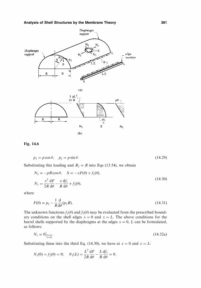
p3 ¼ p cos �; p2 ¼ p sin �: ð14:29ÞSubstituting this loading and R2 ¼ R into Eqs (13.54), we obtain

N2 ¼ �pR cos �; S ¼ �xFð�Þ þ f1ð�Þ;

N1 ¼x2

2R

dF

d�� x

R

df1d�

þ f2ð�Þ;ð14:30Þ

where

Fð�Þ ¼ p2 �1

R

d

d�ðp3RÞ: ð14:31Þ

The unknown functions f1ð�Þ and f2ð�Þ may be evaluated from the prescribed bound-ary conditions on the shell edges x ¼ 0 and x ¼ L. The above conditions for thebarrel shells supported by the diaphragms at the edges x ¼ 0, L can be formulated,as follows:

N1 ¼ 0x¼ox¼L

: ð14:32aÞ

Substituting these into the third Eq. (14.30), we have at x ¼ 0 and x ¼ L:

N1ð0Þ ¼ f2ð�Þ ¼ 0; N1ðLÞ ¼L2

2R

dF

d�� L

R

df1d�

¼ 0:


Fig. 14.6

Thus,

f1ð�Þ ¼L

2Fð�Þ þ C: ð14:33Þ

For a given constant loading along x, we expect that the membrane forces N1 and N2

will be symmetrical, while S will be inversely symmetrical about the shell midspan,i.e., at x ¼ L=2. Thus,

S ¼ 0jx¼L=2 ð14:32bÞSubstituting for p3 and p2 from Eq. (14.29) into Eq. (14.31), we obtain

Fð�Þ ¼ p sin � þ p

RR sin � ¼ 2p sin �; ð14:34Þ

and inserting the above together with Eq. (14.33) into the second Eq. of (14.30), wecan write the expression for S in the following explicit form:

S ¼ �2px sin � þ L

22p sin � þ C ¼ 2p sin �

L

2� x

� �þ C: ð14:35Þ

Applying the condition (14.32b), we obtain

C ¼ 0:

Finally, all the membrane forces for the given loading may be represented in theform

N1 ¼ � px

RðL� xÞ cos �; N2 ¼ �pR cos �; S ¼ 2p

L

2� x

� �sin �: ð14:36Þ

The variation of N1;N2; and S over the depth of the cross section x=L/4of thesemicircular barrel shell under self-weight is shown in Fig. 14.6b.

It follows from Eqs (14.36) that N2 ¼ 0 at � ¼ ��=2. However, the shear forceS does not vanish on the straight edges of the shell, as it is required there for the freeedges. Figure 14.6a shows the variation of the membrane shear forces S from x ¼ 0to x ¼ L at the edge � ¼ �=2. From this diagram, it is seen that these edge forces areself-equilibrating. To resist these forces, the edge members are employed. The latterare loaded by forces equal and opposite to the edge forces on the shell, i.e., S. Sincethe edge shell is compressed by the shear forces S, the edge member is stressed intension only (Fig. 14.6a). Thus, the edge members are subjected to tensile axial loads2pðL=2� xÞ (for � ¼ �=2Þ and they have free ends at the diaphragm supports. Thistensile loading is balanced by the internal axial forces TðxÞ, which are zero at x ¼ 0,L and may be found from the free-body diagram of the part of this edge member. Weobtain from equilibrium the following expressions:

TðxÞ ¼ðx0

2pL

2� x

� �dx ¼ 2p

L

2x� x2

� �:

This force has a maximum at x ¼ L=2, which is given by

Tmax ¼pL2

4:

The total compressive force on the cross section of the shell at x ¼ L=2 may beobtained by substituting x ¼ L=2 into the first Eq. (14.36) and integrating over thecross section. We have, at x ¼ L=2,

382 Chapter 14

R ¼ 2

ð�=20

N1Rd� ¼ � pL2

2

ð�=20

cos �d� ¼ � pL2

2:

It is seen that this unbalanced compressive force on the shell cross section is balancedby the tensile forces Tmax in the two edge beams, which must be provided. Similarly,equilibrium will be satisfied on any other section along the shell span. Thus, asemicircular barrel shell can support dead load under membrane conditions if thetension edge members are provided at their bottom edges. However, the membraneconditions are not satisfied because of the incompatibility of deformations at theshell edges. Indeed, as follows from the first Eq. (14.36), N1 ¼ 0 at �¼� �=2. On theother hand, the edge member has tensile forces TðxÞ, which will cause it to extend inthe axial direction. Moreover, due to its own weight, the edge member will tend todeflect vertically. These deflections will be different from the vertical deformations ofthe shell and edge members. The membrane theory alone cannot eliminate theseincompatibilities of deformations and must be complemented by the bending theory(see Chapter 15).

When a cylindrical shell cross section has edges with an angle � different from90 (e.g., less than 90), there arise further complications associated with an applica-tion of the membrane theory. In fact, in this case, N2 (see the second Eq. of (14.36))will now be nonzero at the longitudinal edges. Thus, the edge member has to resistboth N2 and S forces from the shell edges. This gives rise to further incompatibilitiesof deformation and requires an application of the bending theory of shells.

The procedure for the membrane analysis of cylindrical shells under self-weightdescribed above is a particular case of a more general approach based on a Fourierseries expansion. The governing differential equations for the membrane forces incylindrical shells are given by Eqs (13.50). These equations have constant coefficientsin x and, hence, they can be solved by representing solutions in the form of cosineand sine functions in x.

For barrel shells having simply supported edges x ¼ 0 and x ¼ L, which arecommonly constructed as roof structures, the solutions of Eqs (13.50) can be repre-sented as follows:

N1 ¼X1n¼1

N1n sinn�x

L; S ¼

X1n¼0

Sn cosn�x

L; N2 ¼

X1n¼1

N2n sinn�x

L: ð14:37Þ

It can be shown that the above solutions satisfy the simply supported boundaryconditions. The load components are also expanded into Fourier series in x. Thiscan be done by assuming odd extensions of the loads in the interval (0;L) (refer toAppendix B). Introducing Eqs (14.37) and the load expansions into Eqs (13.50),solutions for membrane stress resultants can be obtained (after solving the resultingordinary differential equations).

14.1.4 Shell roofs in the form of an elliptic or hyperbolic paraboloidcovering rectangular areas

Such a type of roof is commonly used for covering public and sports buildings.Elliptic and hyperbolic paraboloids, considered in this section, fall into the categoryof shells of translation introduced in Sec. 11.7.


At first, assume that an elliptic paraboloid covers a rectangular area with thedimensions 2a 2b and that it is subjected to a uniform vertical surface load ofintensity p3 ¼ p (Fig. 14.7a). The equation of the shell middle surface in this case canbe represented as

z ¼ fx2

2a2þ x2

2a2y2

2b2

!y2: ð14:38Þ

Taking into account, we obtain

@2z

@x2¼ f

a2;@2z

@y2¼ f

b2; and

@2z

@x@y¼ 0:

Assume, for simplicity, that �pp3 � p3 ¼ p, i.e., the vertical surface load per unit area ofthe middle surface is approximately equal to the vertical load of the horizontalprojection of the middle surface. Then, substituting the above into Eq. (13.78), yieldsthe following:

1

b2@2�

@x2þ 1

a2@2�

@y2¼ � p

f: ð14:39Þ

Assume then that the shell edges are attached to supporting arches, so that themembrane forces N1 and N2 are zero and the vertical load is transmitted to thesupports by means of the membrane shear forces. Express these boundary conditionsin terms of the function �. Taking into account the relations (13.77) and (13.72), wecan write the boundary conditions on the shell edges as follows:

384 Chapter 14

Fig. 14.7

N1 ¼ 0 and@2�

@y2¼ 0

x¼�a

; ð14:40aÞ

N2 ¼ 0 and@2�

@x2¼ 0

y¼�b

: ð14:40bÞ

The solution of Eq. (14.39) is sought in the form

� ¼Xn

Cn cosnx coshny�p

2fb2x2; ð14:41Þ

where

n ¼n�

2a; n ¼

n�

2b; n ¼ 1; 3; 5; . . . :

It can be easily shown that � in the form of Eq. (14.41) satisfies exactly the homo-geneous equation (14.39) and the boundary conditions (14.40a). The constants ofintegration Cn are evaluated from the boundary conditions (14.40b). We have

@2�

@x2

y¼�b

¼ � �2

4a2

Xn

n2Cn cosnx coshny�pb2

f¼ 0:

Next, expand the value �pb2=f� �

into the Fourier series

� pb2

f¼Xn

An cosnx; ð14:42aÞ

where

An ¼2

a

ða0

� pb2

f

!cos

n�x

2adx ¼ � 4pb2

�f

1

nsin

n�

2: ð14:42bÞ

Then,

@2�

@x2

y¼�b

¼Xn

� �2

4a2n2 cosh nbCn �

4pb2

�f

1

nsin

n�

2

!cosnx: ð14:43Þ

This expression is equal to zero if

Cn ¼ �16pa2b2 sin n�

2n3�3f coshðn�=2Þ : ð14:44Þ

Introducing Cn from Eq. (14.44) into Eq. (14.41), we obtain the expression for �,that satisfies the differential equation (14.39) and the prescribed boundary conditions(14.40).

Knowing the function �, we can determine �NN1; �NN2; and �SS using the relations(13.55) as follows:


Having determined �, we can calculate �NN1; �NN2; and �NN12 as follows:

�NN1 ¼ �Xn

Cn2n�1 sin n�1x cosn�1y;

�NN2 ¼ �Xn

Cn2n�1 sin n�1x cosn�1y�

pb2

f

�NN12 ¼Xn

Cnn�1n�1 cos n�1x sin n�1y

: ð14:49Þ

Roofs with hyperbolic paraboloid surfaces are commonly made as suspended shells,because in this shape the roof’s state of stress is in good agreement with the moment-less scheme of the analysis.

14.1.5 Asymmetrically loaded domes: wind loading

In the general case of asymmetrically loaded domes, the governing equations of themembrane theory of shells of revolution must be solved without the simplificationsprovided by the axisymmetric membrane theory. As an example of the application ofthe general membrane theory, we consider shells subjected to wind loads.

The value and distribution of the wind loading can be established by testingmodels of structures in wind tunnels. There are special standard relationships thatallow us to determine the value and distribution of wind loading for commonly usedtypes of structures.

It is usual to represent dynamic loading, such as wind and earthquake effects,by statically equivalent for the purposes of design. The wind load on shell struc-tures is composed of pressure on the wind side and suction on the leeward side.Here the load component acting perpendicular to the middle surface p3 is takeninto account. The components p1 and p2 are due to the friction forces and are ofnegligible magnitude. Assuming, for the sake of simplicity, that the wind acts inthe direction of the meridian plane � ¼ 0, the components of the wind pressure areof the form [2]

p1 ¼ p2 ¼ 0; p3 ¼ p sin ’ cos �; ð14:50Þ

where p represents the static wind pressure intensity. Figure 14.8 shows the distribu-tion of the wind load given by Eq. (14.50) on a spherical dome.

The differential equation (13.23) for the wind loading, given by Eq. (14.50), hasthe following form (making n ¼ 1):

1

R1R2 sin ’

d

d’

R22 sin ’

R1

dU1

d’

!� U1

R1 sin2 ’

¼ F1ð’Þ; ð14:51Þ

where

F1ð’Þ ¼ �p1

R1R2 sin ’

d

d’R3

2 sin3 ’ cos ’

� �� R2 sin ’

� �: ð14:52Þ


N1 ¼ � p

R22 sin

3 ’C1

ð’’0

R1 sin �’’d �’’þð’’0

�ð �’’ÞR1 sin �’’d �’’þ C2

� �cos �; ð14:58Þ

N2 ¼ �p R2 sin ’�1

R1R2 sin3 ’

C1

ð’’0

R1 sin �’’d �’’

�

þð’’0

�ð �’’ÞR1 sin �’’d �’’þ C2

��cos �: ð14:59Þ

Knowing U1, we can determine V1 from the first Eq. (13.11). We have the following

@V

@�¼ �p3R

32 sin

2 ’ cos ’� R22 sin ’

R1

@U

@’¼ �p

R3

2 sin3 ’ cos ’

� C1 R2 sin ’� cot ’

ð’’0

R1 sin �’’d �’’

� ��þ�ð’ÞR2 sin ’

� cot ’

ð’’0

�ð �’’ÞR1 sin �’’d �’’� C2 cot ’

��cos �:

Taking into account the second relation (13.10), we obtain the following (againdropping the superscript 1 for the membrane shear force):

S ¼ V

R22 sin

2 ’¼ �p R2 sin ’� C1

1

R2 sin ’� cos ’

R22 sin

3 ’

ð’’0

R1 sin �’’d �’’

!"

� �ð’ÞR2 sin ’

þ cos ’

R22 sin

3 ’

ð’’0

�ð �’’ÞR1 sin �’’d �’’þ C2 cos ’

R22 sin

3 ’

#sin �:

ð14:60Þ

The constants of integration, C1 and C2, are to be evaluated by assigning the mem-brane forces N1 and N2 on the upper edge of the shell, i.e., at ’ ¼ ’0. Denoting theseforces by N

ð0Þ1 and Sð0Þ, and letting ’ ¼ ’0 in Eqs (14.58) and (14.60), we obtain the

following expressions:

C1 ¼ � 1

pN

ð0Þ1 R

ð0Þ2

� �2sin ’0 cos ’0 � Sð0ÞRð0Þ

2 sin ’0

� �;

C2 ¼ �R

ð0Þ2

� �2sin3 ’0

� �p

Nð0Þ1 :

ð14:61Þ

For domes closed at the vertex, we have ’0 ¼ 0 and C1 ¼ C2 ¼ 0.As an example, let us determine the expressions for the membrane forces for a

spherical dome of radius R (see Fig. 14.8). For this particular case, R1 ¼ R2 ¼ R;’0 ¼ 0 and


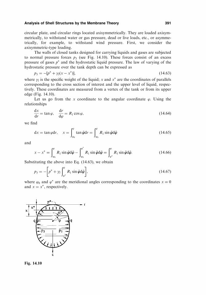
circular plate, and circular rings located axisymmetrically. They are loaded axisym-metrically, to withstand water or gas pressure, dead or live loads, etc., or asymme-trically, for example, to withstand wind pressure. First, we consider theaxisymmetric-type loading.

The walls of closed tanks designed for carrying liquids and gases are subjectedto normal pressure forces p3 (see Fig. 14.10). These forces consist of an excesspressure of gases p and the hydrostatic liquid pressure. The law of varying of thehydrostatic pressure over the tank depth can be expressed as

p3 ¼ � p þ �lðx� x Þ½ �; ð14:63Þwhere �l is the specific weight of the liquid; x and x are the coordinates of parallelscorresponding to the cross section of interest and the upper level of liquid, respec-tively. These coordinates are measured from a vertex of the tank or from its upperedge (Fig. 14.10).

Let us go from the x coordinate to the angular coordinate ’. Using therelationships

dx

dr¼ tan ’;

dr

d’¼ R1 cos ’; ð14:64Þ

we find

dx ¼ tan ’dr; x ¼ð’’0

tan �’’dr ¼ð’’0

R1 sin �’’d �’’ ð14:65Þ

and

x� x ¼ð’’0

R1 sin �’’d �’’�ð’ ’0

R1 sin �’’d �’’ ¼ð’’ R1 sin �’’d �’’: ð14:66Þ

Substituting the above into Eq. (14.63), we obtain

p3 ¼ � p þ �lð’’ R1 sin �’’d �’’

� �; ð14:67Þ

where ’0 and ’ are the meridional angles corresponding to the coordinates x ¼ 0and x ¼ x , respectively.


Fig. 14.10

The meridional forces for tanks can be determined from Eq. (13.33b) and Eq.(13.39). The former equation can be rewritten for tanks, taking into account Eq.(14.67) and noting that p1 ¼ 0, as follows:

N1 ¼1

R2 sin2 ’

p ð’’0

R1R2 cos �’’ sin �’’d �’’

�

þ�lð’’0

R1R2 cos �’’ sin �’’d �’’

ð’’ R1 sin �’’d �’’

�þN

ð0Þ1 R

ð0Þ2 sin2 ’0

R2 sin2 ’

ð14:68Þ

If we take into account relation (13.6b), then the first integral in the square bracketscan be represented as follows:ð’

’0

R2 sin �’’ � dðR2 sin �’’Þ ¼ 1

2R2

2 sin2 ’� ðRð0Þ

2 Þ2 sin2 ’0� �

:

Then, Eq. (14.68) appears as

N1 ¼p R2

2þ �l

R2 sin2 ’

ð’’ R1R2 cos �’’ sin �’’d �’’

ð’’ R1 sin �’’d �’’

þ Nð0Þ1 � p Rð0Þ

2

2

!R

ð0Þ2 sin2 ’0

R2 sin2 ’

:

ð14:69Þ

In the second term of Eq. (14.69), the lower limit of the first integral is ’ ; becausefor ’ < ’ the hydrostatic pressure of the liquid is zero.

Below we consider the membrane analysis of liquid storage facilities made ofvarious forms of shells of revolution under axisymmetric and asymmetric loads.

14.2.2 Spherical storage tank with supports in its diametrical plane:axisymmetric loading

For a closed spherical shell R1 ¼ R2 ¼ Rð0Þ1 ¼ R

ð0Þ2 ¼ R and ’0 ¼ 0. Then, it follows

from Eq. (14.69) that

N1 ¼p R2

þ �lR2

6 sin2 ’cos3 ’ � cos2 ’ 3 cos ’ � 2 cos ’ð Þ� �

: ð14:70Þ

Since the meridional forces N1 have an obvious abrupt change at the support(’ ¼ �=2), Eq. (14.70) is valid for ’ < �=2.

The circumferential force can be found from Eq. (13.39) as follows:

N2 ¼ �ðp3RþN1Þ; ð14:71Þwhere

p3 ¼ p þ �lRð’’ sin �’’d �’’ ¼ p þ �lRðcos ’ � cos ’Þ:

Let us determine the meridional forces in the lower portion of the sphere tank, i.e.,for ’ > �=2. Taking the lower vertex of the sphere as a reference point for thereading of the meridional angles ’, we replace the lower limit in the first integralof Eq. (14.69) with �, i.e., ’0 ¼ �. We obtain the following:

392 Chapter 14

N1 ¼p R2

þ �lR2

sin2 ’

ð’�

cos �’’ sin �’’d �’’

ð’’ sin �’’d �’’ ¼ p R

2

þ �lR2

63 cos ’ þ 2

1þ cos3 ’

sin2 ’

! ð14:72Þ

It follows from Eq. (14.70) that, at the support, for ’ ¼ �=2, we derive

N01 ¼

p R2

þ �lR2

6cos3 ’ :

On the other hand, from Eq. (14.72), for ’ ¼ �=2, the meridional force is

N001 ¼ p R

2þ �lR

2

6ð3 cos ’ þ 2Þ:

Thus, the value of the abrupt change in the meridional force at the support level inthe diametrical plane is

�N1 ¼ N001 �N

01 ¼

�lR2

6ð3 cos ’ þ 2� cos3 ’ Þ: ð14:73Þ

In particular, if the spherical tank is completely filled by a liquid only, i.e., p ¼ 0and ’ ¼ 0, then

�N1 ¼2

3�lR

2: ð14:74aÞ

Recalling that the volume of the sphere is V ¼ 4

3�R3, we can rewrite Eq. (14.74a), as

follows:

�N1 ¼V�l2�R

: ð14:74bÞ

The above represents the meridional force, which balances the liquid weight fillingthe spherical tank. Thus, the meridional forces N1 at the sphere portion 0 � ’ < �=2are to be determined from Eq. (14.70) and at the portion �=2 � ’ � � from Eq.(14.72). The circumferential force N2 is determined from Eq. (14.71) for both por-tions of the sphere, taking into account that N1 for the upper and lower portions aregiven by Eqs (14.70) and (14.72), respectively. It is seen from the above equationsthat the maximum values of the meridional forces take place when the sphericalstorage tank is completely filled by a liquid.

Determine the limit of the second term in parentheses of Eq. (14.72) when’! �. Using the L’Hospital’s rule, we obtain

N1

’¼�¼

p R2

þ �lR2

2ð1þ cos ’ Þ: ð14:75Þ

With the use of Eq. (14.71), it will be easily established that

N1j’¼� ¼ N2j’¼�:The meridional and circumferential force, N1 and N2, diagrams for the sphericalstorage tank filled completely by a liquid of a specific weight �l are shown in Fig.14.11.


jointly by the edge zones of the roof and the wall near the junction. A more accuratestress analysis of such a junction, including the moment shell theory, is given in thenext chapter.

The water load acting on the cylindrical part of the tank causes the circumfer-ential membrane forces only, N

ðsÞ2 . It is equal to

NðsÞ2 ¼ �lax; ð14:88aÞ

where �l is the water density. The maximum compressive meridional force NðsÞ1

occurs at the base of the cylinder and is

NðsÞ1max ¼ V1 þ �chsL; ð14:88bÞ

where �c and hs are the concrete density and the wall thickness of the cylinder,respectively. The maximum circumferential force acts at the base of the cylinder.It is equal to

NðsÞ2max ¼ �laL: ð14:88cÞ

Ring beam

At the top of the cone, the meridional compressive force NðsÞ1max is given by Eq.

(14.88b). Neglecting the self-weight of the ring, this force is directly applied to thetop of the cone, as shown in Fig. 14.14b. The above force can be resolved into acomponent along the cone, N

ðcÞ1 ¼ N

ðsÞ1max= sin , and the horizontal component,

H2 ¼ NðsÞ1max cot . The latter component is resisted by the ring beam. The hoop

tension in the ring beam is given by

T ðrÞ ¼ H2ðaþ d=2Þ:

Conical shell

The conical shell is subjected to dead and water loads. The dead load consists of theself-weight of the conical frustum, Wc, and the total vertical load carried on top ofthe cone, which comes from the roof shell and the cylindrical wall, Ws. The aboveload components are

Wc ¼ Uchc�c

where Uc ¼ �ðaþ rÞ x2 þ a� rð Þ2� �1=2 ð0 � � l) is the volume of the frustum, hc isthe cone thickness, and r is the radius of the cone parallel circle of interest;

Ws ¼ NðsÞ1max2�ðaÞ:

Then, the meridional force due to dead load and carried by the cone, NðcÞ1D, is given by

NðcÞ1D ¼ � Wc þWs

2�rðsin Þ : ð14:89aÞ

The circumferential force in the cone shell, NðcÞ2D due to the dead load, can be obtained

from the third Eq. (13.7) by letting R1 ¼ 1 and p3 ¼ �chc cos.The water load components are (using the coordinates s and where s is

measured along line OB starting from point O, as shown in Fig. 14.14b)

p1 ¼ 0; p3 ¼ ��l Lþ ðS � sÞ sin ½ �: ð14:90Þ


N2 ¼ �p3R ¼ �p RXn

pn cos n�: ð14:94aÞ

Then, taking into account that R2 ¼ R; p2 ¼ 0; and f1ð�Þ ¼ 0 (due to theboundary conditions described above), we obtain from Eq. (13.52b) the following:

S ¼ �ðx0

dð�p3RÞRd�

d �xx ¼ �p � xXn

pnn sin n� ð14:94bÞ

From Eq. (13.52c) it follows that (letting f2ð�Þ ¼ 0 and p1 ¼ 0)

N1 ¼ �ðx0

1

R

@S

@�d �xx ¼ p x2

2R

Xn

pnn2 cos n�: ð14:94cÞ

In Eqs (14.94b) and (14.94c), the unknown functions f1ð�Þ and f2ð�Þ are equal to zerodue to the prescribed boundary conditions (14.93). The diagrams of the membraneforces N1;N2; and S are shown in Fig. 14.15b at a section x ¼ H. The circumfer-ential force N2 is a constant over the shell depth in the membrane theory. However,it should be noted that when we approach the supporting cross section, the bendingaffects the state of stress significantly. Consequently, the membrane forces N1;N2;and S are redistributed over the length and cross sections of the shell.

14.3 AXISYMMETRIC PRESSURE VESSELS

Pressure vessels are commonly used to resist internal pressure (pressurized liquids orgases). They are usually made of metals or composite materials. In such construc-tions, the stresses due to the self-weight of the vessel are negligible compared with thestresses due to the internal pressure.

Let us consider a pressure vessel in the form of a shell of revolution with anarbitrary shape of the meridian, which intersects the axis of revolution at a rightangle (Fig. 14.16).

In this section, we determine the membrane forces due to the axisymmetricinternal pressure, p. Thus, the applied load components are

p1 ¼ 0; p2 ¼ 0; and p3 ¼ �p:

402 Chapter 14

Fig. 14.16

where �c and �s are the radial displacements of the cylinder and sphere, respectively,at the above-mentioned neighboring points.

It follows from Eqs (14.96), that the radial displacement of the cylinder isgreater than that of the sphere. Hence, in order to provide the compatibility ofthe radial displacements at the junction of the two shells, the shear forces, V , andbending moments,M, are to be applied at this junction, as shown in Fig. 14.17b. Thesituation becomes more complicated if we have a shallow spherical shell instead of ahemispherical shell as a head. In this case, the radial membrane force N1 in thesphere, at the junction with the cylinder, has to be restricted by the cylinder as anedge load. Consequently, the displacement of the two shells is much greater and aring beam needs to be provided at the junction to resist the radial membrane forceN1. The actual state of stress at the above junction will be discussed in detail in thenext chapter.

A toroidal shell is also used for pressure vessels. A toroid is generated by therotation of a closed curve about an axis passing outside. Figure 14.18a shows a shellin the shape of a toroid or doughut of circular section subjected to internal pressurep. The membrane force N1 may be found from conditions of equilibrium of a shellsegment shown in Fig. 14.18b, i.e.,

N1ð2�rÞ sin ’ ¼ p�ðr2 � b2Þ;

from which

N1 ¼p

2� r

2 � b2

r sin ’:

Taking into account that r ¼ bþ a sin ’, we represent N1 in the form

N1 ¼pa

2

2bþ a sin ’

bþ a sin ’: ð14:97aÞ

404 Chapter 14

Fig. 14.18

The circumferential membrane force N2 may be found from Eq. (13.39); substituting

there R1 ¼ a;R2 ¼ aþ b

sin ’and p3 ¼ �p, we have

N2 ¼ � p3R2 þN1

R2

R1

� �¼ pR2 �N1

R2

R1

¼ 1

2pa: ð14:97bÞ

The radial displacement w can be determined in the usual fashion, i.e.,

w ¼ r"2 ¼r

EhðN2 � #N1Þ:

However, if we try to calculate the longitudinal component of the displacement,which is parallel to the axis of the shell, u, one can show that the integral in theexpression (13.43) diverges, since its integrand approaches infinity as ’ goes to zero.It follows from the above that in the domain of the shell near a point ’ ¼ 0, themembrane theory does not describe the state of stress and strain of the toroidal shell,even loaded by a uniform pressure.

PROBLEMS

14.1 A hemispherical roof dome in Fig. 14.1 is subjected to its own weight. Assume that the

dome is constructed of masonry having a radius of curvature R ¼ 40m. Determine the

required thickness of the dome according to the maximum principal stress theory if the

compressive ultimate stress �u ¼ 22MPa and the factor of safety is 1.9.

14.2 A spherical roof dome in Fig. 14.2 is subjected to its own weight. Determine the

required cross-sectional area of the thrust ring. Take R ¼ 35m; ’1 ¼ 55; and hs ¼10 cm (thickness of the dome). Assume that the dome and the thrust ring are con-

structed of concrete with � ¼ 0:15.14.3 A planetarium dome may be approximated as an edge-supported truncated cone, as

shown in Fig. 14.5b. It is subjected to a snow load with a maximum accumulation over

the dome q ¼ 2:5 kPa. Assume that the dome is constructed of 12 cm thick concrete

having the radii of the parallel circles equal to 40 m at the base and 25 m at the top,

respectively. Determine the membrane stresses in the dome.

14.4 A cooling tower may be approximated by a one-sheet hyperboloid of revolution (see

Fig. 11.9f). The equation of its meridian is r ¼a

b

ffiffiffiffiffiffiffiffiffiffiffiffiffiffiffib2 þ z2

p, where a and b are the

parameters of the hyperbola. Determine the membrane forces, N1 and N2, distribution

over the depth of the cooling tower under its own weight. Assume that the tower is

made of concrete and T ¼ 22:0m; S ¼ 116:0m; a ¼ 51:5m; b ¼ 73:42m; and

h ¼ 0:2m.

Hint: use cylindrical coordinates for the solution.

14.5 The four different dome configurations of the same height, H ¼ 0:5a, are shown in Fig.

P.14.1. The first dome is spherical with R0 ¼ R ¼ 1:25a; the second dome is parabolic

with R0 ¼ a; the third dome has the form of a semiellipsoid with R0 ¼ 2a and �¼ 3;

and the fourth dome represents a segment of ellipsoid (the tangents of the dome

meridian at its edges are not vertical) with R0 ¼ 1:625a and � ¼ 1:5. All the four

domes cover the same areas (of radius a) and they are made of concrete. (a) Find

the meridional and circumferential forces distribution over the height of the above

domes under their self-weight p in terms of a and p. (b) Determine the cross-sectional

area of the thrust ring for all domes if the ring is assumed to be also made of the

reinforced concrete. Take the thickness of the shell h ¼ a=50 and �c ¼ 0:15. (c) Analyze


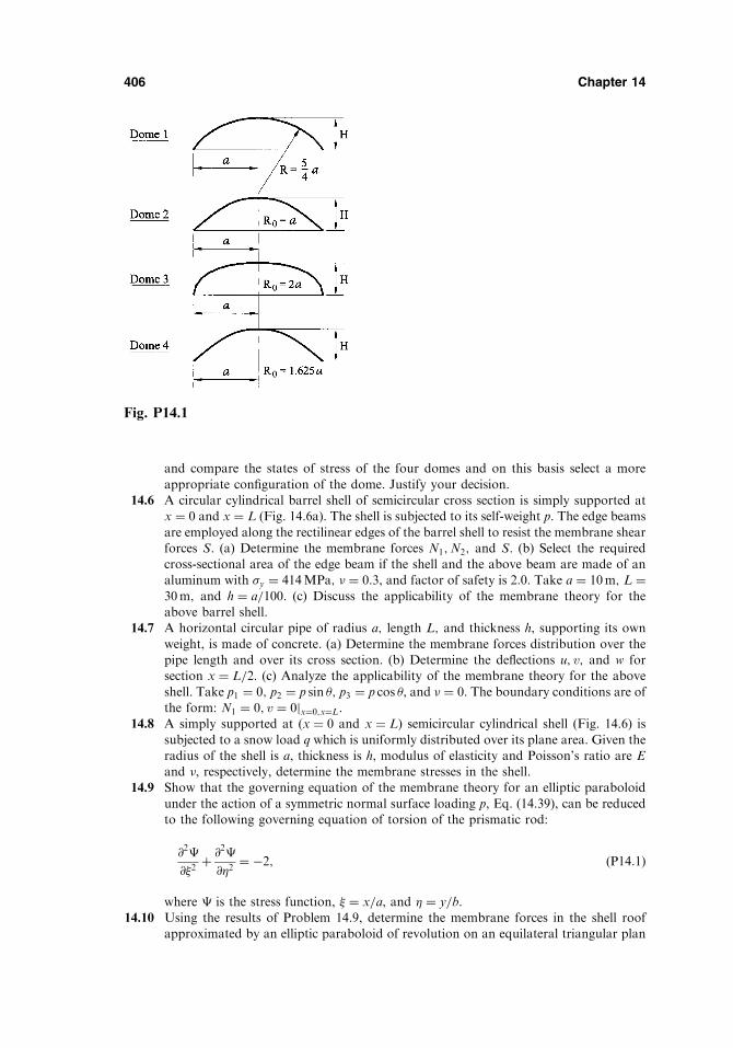
and compare the states of stress of the four domes and on this basis select a more

appropriate configuration of the dome. Justify your decision.

14.6 A circular cylindrical barrel shell of semicircular cross section is simply supported at

x ¼ 0 and x ¼ L (Fig. 14.6a). The shell is subjected to its self-weight p. The edge beams

are employed along the rectilinear edges of the barrel shell to resist the membrane shear

forces S. (a) Determine the membrane forces N1;N2; and S. (b) Select the required

cross-sectional area of the edge beam if the shell and the above beam are made of an

aluminum with �y ¼ 414MPa; � ¼ 0:3, and factor of safety is 2.0. Take a ¼ 10m; L ¼30m; and h ¼ a=100. (c) Discuss the applicability of the membrane theory for the

above barrel shell.

14.7 A horizontal circular pipe of radius a; length L; and thickness h, supporting its own

weight, is made of concrete. (a) Determine the membrane forces distribution over the

pipe length and over its cross section. (b) Determine the deflections u; v; and w for

section x ¼ L=2. (c) Analyze the applicability of the membrane theory for the above

shell. Take p1 ¼ 0; p2 ¼ p sin �; p3 ¼ p cos �, and � ¼ 0. The boundary conditions are of

the form: N1 ¼ 0; v ¼ 0jx¼0;x¼L.

14.8 A simply supported at ðx ¼ 0 and x ¼ LÞ semicircular cylindrical shell (Fig. 14.6) is

subjected to a snow load q which is uniformly distributed over its plane area. Given the

radius of the shell is a, thickness is h, modulus of elasticity and Poisson’s ratio are E

and �, respectively, determine the membrane stresses in the shell.

14.9 Show that the governing equation of the membrane theory for an elliptic paraboloid

under the action of a symmetric normal surface loading p, Eq. (14.39), can be reduced

to the following governing equation of torsion of the prismatic rod:

@2�

@�2þ @

2�

@ 2¼ �2; ðP14:1Þ

where � is the stress function, � ¼ x=a, and ¼ y=b.14.10 Using the results of Problem 14.9, determine the membrane forces in the shell roof

approximated by an elliptic paraboloid of revolution on an equilateral triangular plan

406 Chapter 14

Fig. P14.1

(Fig P.14.2) due to a dead load p: Assume reasonable values for any additional proper-

ties and parameters required.

Hint: it is known from the theory of elasticity that the stress function � for the torsion

of the rod having a cross section in the form of an equilateral triangle is expressed in

the following form:

� ¼ � 1

6ax3 � 3xy2� �� 2

3a2 þ 1

2ðx2 þ y2Þ

� �: ðP:14:2Þ

14.11 An auditorium dome of span 350 ft is approximated by a spherical shell of radius

280 ft. The dome is simply supported at its ends. Determine the maximum membrane

forces in the dome under the action of a wind pressure. The components of the wind

pressure are given by Eqs (14.50) and p ¼ 15 psf. Assume reasonable values for any

additional properties required.

14.12 A circular cylindrical chimney shell of height L and radius R is subjected to a wind

pressure p3. The chimney shell is fixed at its base and free at the top. Assuming that the

wind pressure is constant over the height of the chimney and in the circumferential

direction is approximated by the polynomial p3 ¼ pð�0:7þ 0:5 cos � þ 1:2 cos 2�Þ,determine the membrane forces in the shell.

14.13 A steel cylindrical pressure vessel with conical end caps is subjected to an internal

pressure of p ¼ 1:5 MPa, as shown in Fig. P.14.3. Using the membrane theory

alone, determine the required thickness of the cylinder if the yield stress of the steel

is 250 MPa. Where may additional strengthening be required?

14.14 The tank shown in Fig. P.14.4 has a cylindrical top and a conical bottom. The tank is

supported by a structure (not shown) that applies only vertical forces around the

parallel AB. The tank is filled to depth H ¼ 2:5R with water of weight density �l .Determine the expressions for the membrane forces just above and just below the

parallel AB.

14.15 Redo Problem 14.14 replacing the conical bottom with a hemispherical bottom of

radius R. Consider two cases: (a) the bottom convexity is directed down and (b) the

bottom convexity is directed up.

14.16 The spherical tank is filled with water at a distance H from the top, as shown in Fig.

P.14.5a. The tank is supported by the outlet pipe. Determine the expressions for the

membrane forces if the radius of the tank is R and water density is �l

Hint: the volume of a spherical segment is U ¼ �l

6ð3r2A þ 3r2B þ l2Þ; 0 < l < 2R.


Fig. P14.2

14.17 A horizontal circular pipe of radius R; length l; and thickness h is subjected to internal

gas pressure p. Determine the membrane stresses in the pipe if its ends are assumed to

be built-in.

14.18 The Intze tank, shown in Fig. 14.14a, is filled with water up to the top of the cylindrical

wall. The tank is made of concrete. The total load on the roof shell is taken as p ¼ 3:5kPa over its surface area. Determine (a) the membrane stresses in the roof shell,

cylindrical wall, conical shell, and bottom shell; (b) the tension forces in the ring

beam at the junction of the wall and cone, and in the supporting ring beam. Let a ¼7:6m; L ¼ 7:2m, b ¼ 4:8m; f1 ¼ 2:0m; f2 ¼ 1:3m; hr ¼ 95mm, hs ¼ 250mm; and hb¼ 280mm

408 Chapter 14

Fig. P14.3

Fig. P14.4

Fig. P14.5

14.19 A circular toroidal shell is subjected to internal pressure p ¼ 2:5MPa, as shown in Fig.

14.18. The dimensions of the toroid are a ¼ 0:09m; b ¼ 0:60m; and h ¼ 1:8mm.

Determine the membrane stresses in the shell.

14.20 A spherical concrete dome having a span of 2a and height H (H ¼ 0:5aÞ supports itsown weight p. The ends of the dome have roller supports (they can freely displace in the

horizontal direction). Determine (a) the horizontal displacements at the dome base and

(b) the vertical displacement at its apex.

14.21 Redo Problem 14.20, except now assume that the dome is subjected to snow loading q.

REFERENCES

1. Novozhilov, V.V., The Shell Theory [translated from 2nd Russian edn by P.G. Lowe],

Noordhoff, Groningen, The Netherlands, 1964.



3. Gere, J.M. and Timoshenko, S.P., Mechanics of Materials, 4th edn, PWS Publishing

Company, Boston, 1997.


of shells employed in engineering. A cylindrical shell, as mentioned previously, issuccessful in combining simplicity, compactness, and almost an ideal technologicaleffectiveness. The latter enables one to develop items by usual rolling-up a givensheet skelps. Therefore, pattern cutting of a material and the subsequent process ofmanufacturing of a given structural form requires a minimum of technologicaleffort. On the other hand, unlike the other shell forms – say, noncircular shells ofrevolution – the governing differential equations of the moment theory of a circularcylindrical shell of constant thickness represent a system of equations with constantcoefficients, which gives us the possibility to analyzing their solutions in the generalform.

15.2 CIRCULAR CYLINDRICAL SHELLS UNDER GENERAL LOADS

Here we will use the same coordinates x and � as we did for the membrane theory ofcylindrical shells (Fig. 11.13), where x is the distance of a point of interest from adatum plane normal to the generators (this plane usually coincide with one edge ofthe shell) and � measures the angular distance of the point from a datum generator.In this case, the Lame parameters are given by Eqs (11.53) and the principal radii ofcurvature are

R1 ¼ 1; R2 ¼ R: ð15:1Þ

The equilibrium equations of the general classical shell theory, Eqs.(12.41) and(12.42), and the relations (12.43), appear in the following form:

R@N1

@xþ @S@�

þ p1R ¼ 0;

@N2

@�þ R

@S

@x�Q2 �

@H

@xþ p2R ¼ 0;

@Q2

@�þ R

@Q1

@xþN2 þ p3R ¼ 0; ð15:2Þ

@M2

@�þ R

@H

@x� RQ2 ¼ 0;

R@M1

@xþ @H@�

� RQ1 ¼ 0: ð15:3Þ

This system of five differential equations of equilibrium can be reduced to the fol-lowing system of three equations, by eliminating the shear forces, Q1 and Q2, fromEqs (15.3):

R@N1

@xþ @S@�

þ p1R ¼ 0;

@N2

@�þ R

@S

@x� 1

R

@M2

@�� 2

@H

@xþ p2R ¼ 0;

1

R

@2M2

@�2þ 2

@2H

@x@�þ R

@2M1

@x2þN2 þ p3R ¼ 0:

ð15:4Þ

412 Chapter 15

a2 ¼ h2=12R2 ð15:10ÞFor thin shells the values of a2 are very small (10�4–10�6). These are the

governing differential equations for the displacements in circular cylindrical shellsunder general loading.

Following Gol’denveizer [1] the problem of solving Eqs (15.7) is reduced to theintegration of a single differential equation for some potential function. For thispurpose, it is convenient to use the operator method introduced in [1]. Noting thatthe coefficients of Eqs. (15.7) are constants; we will consider those relations, accordingto the above method, as algebraic equations in u; v; and w. These have coefficients inwhich the symbols of differentiation, @k=@�k and @k=@�k ðk ¼ 1; 2; 3; 4Þ occur togetherwith other quantities (the symbol of multiple differentiation is to be considered as theproduct of appropriate degrees of @=@� and @=@�). Let us set these as follows:

u ¼ 11�1 þ12�2 þ13�3; v ¼ 21�þ22�2 þ23�3;

w ¼ 31�1 þ32�2 þ33�31;ð15:11Þ

where

¼l11 l12 l13l21 l22 l23l31 l32 l33

24

35 ð15:12Þ

is the determinant made up of the operators given by Eq. (15.7) and ik ði; k ¼1; 2; 3Þ are the minors of the above determinant, i.e., the determinants obtainedby excluding the ith and the kth column from ik.

Substituting the expressions (15.11) into Eqs (15.7) and using the well-knowntheorems of the theory of linear algebraic equations, one finds the following rela-tions:

�1 þ g1 ¼ 0; �2 þ g2 ¼ 0; �3 þ g3 ¼ 0: ð15:13ÞEquations (15.13) are nonhomogeneous. Their solutions can be represented in theform

�1 ¼ �10 þ�11; �2 ¼ �20 þ�21; �3 ¼ �30 þ�31; ð15:14Þwhere the second subscript 0 refers to the solutions of the homogeneous equations(complementary solutions) and the second subscript 1 stands for particular solu-tions. The former solutions of Eqs (15.13) are found from the following equations:

�10 ¼ 0; �20 ¼ 0; �30 ¼ 0: ð15:15ÞThus, the functions u0; v0; and w0 are defined as

u0 ¼ 11�10 þ12�20 þ13�30; v0 ¼ 21�10 þ22�20 þ23�30;

w0 ¼ 31�10 þ32�20 þ33�30

ð15:16ÞThey correspond to solutions of the homogeneous equations (15.7) for any �10;�20;and �30 that satisfy Eqs (15.15). In particular, we can let

�10 ¼ 0; �20 ¼ 0; �30 ¼2

1� �F : ð15:17Þ

414 Chapter 15

Then, each solution of the equation

F ¼ 0 ð15:18Þcorresponds to an integral of the homogeneous equations (15.7), given by the expres-sions

u0 ¼2

1� �13F; v0 ¼2

1� �23F; w0 ¼2

1� �33F; ð15:19Þ

or using the explicit form of the symbols 13;23; and 33 from Eqs (15.9) and(15.12), we obtain

u0 ¼ � @3

@�@�2:þ � @

3

@�3þ a2

ð1þ �Þð2� �Þ1� � :

@5

@�3@�2þ 1þ �1� �

@5

@�@�4þ 4�

@3

@�3

"(

þ 2�

1� �@3

@�@�2

#)F;

v0 ¼ ð2þ �Þ @3

@�2@�þ @3

@�3� a2

2ð2� �Þ1� �

@5

@�4@�þ 4� 3�þ �2

1� �@5

@�2@�3þ @5

@�5

" #( )F;

w0 ¼@4

@�4þ 2

@4

@�2@�2þ @4

@�4þ a2 4

@4

@�4þ 2ð2� 2�þ �2Þ

1� �@4

@�2@�2þ @4

@�4

" #( )F :

ð15:20ÞSubstituting for the operators lik from the relations (15.9) into (15.12) and (15.18), weobtain the latter equation in the explicit form, as follows:

ð1þ 4a2Þ @8F

@�8þ 4ð1þ a2Þ @8F

@�6@�2þ 6þ a2ð1� �2Þ� � @8F

@�4@�4þ 4

@8F

@�2@�6þ @

8F

@�8

þ ð8� 2�2Þ @6F

@�4@�2þ 8

@6F

@�2@�4þ 2

@6F

@�6þ ð1� �2Þ 1

a2þ 4

� �@4F

@�4

þ 4@4F

@�2@�2þ @

4F

@�4¼ 0:

ð15:21ÞThus, the problem is reduced to funding solutions of one single eighth-order dif-ferential equation (15.21) and the function F can be considered as a potentialfunction for the integration of the homogeneous equations (15.7). Solving Eq.(15.21), we can determine the function F and then, using the relations (15.20),find the complementary solutions, u0; v0; and w0. The particular solutions fornonhomogeneous equations (15.7), u1; v1; and w1, can be reduced to determiningthe particular integrals for the nonhomogeneous equations (15.13). In many cases,the particular solutions can be obtained from the membrane theory introduced inChapter 13.

Moment Theory of Circular Cylindrical Shells 415

ordinary linear differential equation with constant coefficients. We present thisequation for the function Fn:

dnðFnÞ � ð1þ 4a2Þ d8Fn

d�8� 4ð1þ a2Þn2 d

6Fn

d�6þ�6n4 þ a2ð1� �2Þn4:� ð8� 2�2Þn2

þ ð1� �2Þ 1

a2þ 4

� ��d4Fn

d�4� 4n2ðn2 � 1Þ2 d

2Fn

d�2þ n4ðn2 � 1Þ2Fn ¼ 0:

ð15:24ÞIts solution can be represented in the form

Fn ¼ Ae�� ðA¼ constÞ:Inserting the above into Eq. (15.24) and neglecting small quantities of the order of a2

in comparison with those of order unity in its coefficients, yields the followingcharacteristic equation for determining roots �:

�8 � 4n2�6 þ 6n4�4 � ð8� 2�2Þn2�4 þ ð1� �2Þa�2�4 � 4n2ðn2 � 1Þ2�2

þ n4ðn2 � 1Þ2 ¼ 0:ð15:25Þ

The detailed investigation of the roots of this equation and the corresponding ana-lysis of the state of stress and strain of closed cylindrical shells has been carried outby Gol’denveizer [1]. In particular, it was shown in the above reference that ifn � a�1=2 ¼ ffiffiffiffiffi

12p

R=h, the roots of the characteristic equation are broken downinto small ( �j j � a1=2n2) and large ( �j j � a�1=2) roots. The above inequality holdsfor closed cylindrical shells having a large and an intermediate relative reducedlengths, L=R. The small roots correspond to the basic state of stress for the shell,described by the simplified equations of the semi-membrane theory of shells (Sec.

17.2). By the way, if the relative length is not too large, so that L=R <0:8

n2

ffiffiffiffiR

h

r, the

membrane theory can also be applied to describe a slowly varying state of stress. Thelarge roots correspond to the edge effect state of stress described by simplifiedequations introduced in Sec. 17.5. Both the approximate theories mentioned aboveare introduced and analyzed in Chapter 17.

If n � a�1=2, the above division of the roots into the small and large is impos-sible. The above inequality holds for closed cylindrical shells having a small and verysmall reduced length L=R. These shells are in a complete state of stress, which cannotbe uncoupled into the previously introduced elementary stress states. However, foran analysis of these shells under general loading, the Donnell–Mushtari–Vlasovapproximate theory, introduced in Sec. 17.3, can be applied. According to thattheory, the characteristic equation (15.25) may be simplified significantly. It haseight mutually complex conjugate roots of the form

�1�4 ¼ �p1 � iq1; �5�8 ¼ �p2 � iq2;

where p1; q1; p2; and q2 are real positive numbers. To eliminate the complexquantities, the arbitrary constants are replaced according to the followingexpressions:


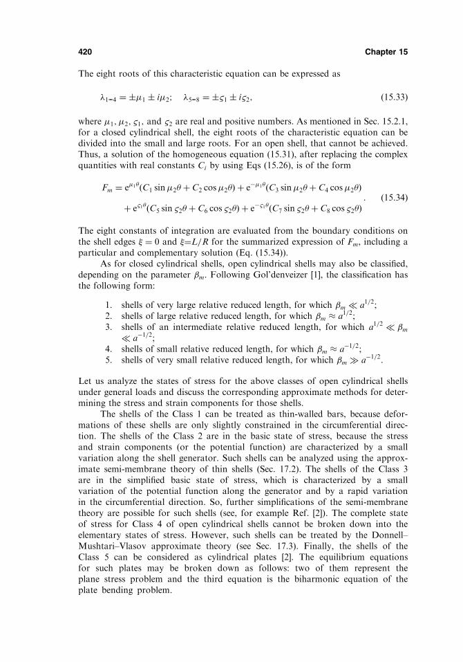
The eight roots of this characteristic equation can be expressed as

�1--4 ¼ ��1 � i�2; �5--8 ¼ �&1 � i&2; ð15:33Þ

where �1; �2; &1; and &2 are real and positive numbers. As mentioned in Sec. 15.2.1,for a closed cylindrical shell, the eight roots of the characteristic equation can bedivided into the small and large roots. For an open shell, that cannot be achieved.Thus, a solution of the homogeneous equation (15.31), after replacing the complexquantities with real constants Ci by using Eqs (15.26), is of the form

Fm ¼ e�1�ðC1 sin�2� þ C2 cos�2�Þ þ e��1�ðC3 sin�2� þ C4 cos�2�Þ

þ e&1�ðC5 sin &2� þ C6 cos &2�Þ þ e�&1�ðC7 sin &2� þ C8 cos &2�Þ: ð15:34Þ

The eight constants of integration are evaluated from the boundary conditions onthe shell edges � ¼ 0 and �¼L=R for the summarized expression of Fm, including aparticular and complementary solution (Eq. (15.34)).

As for closed cylindrical shells, open cylindrical shells may also be classified,depending on the parameter m. Following Gol’denveizer [1], the classification hasthe following form:

1. shells of very large relative reduced length, for which m � a1=2;2. shells of large relative reduced length, for which m � a1=2;3. shells of an intermediate relative reduced length, for which a1=2 � m

� a�1=2;4. shells of small relative reduced length, for which m � a�1=2;5. shells of very small relative reduced length, for which m � a�1=2.

Let us analyze the states of stress for the above classes of open cylindrical shellsunder general loads and discuss the corresponding approximate methods for deter-mining the stress and strain components for those shells.

The shells of the Class 1 can be treated as thin-walled bars, because defor-mations of these shells are only slightly constrained in the circumferential direc-tion. The shells of the Class 2 are in the basic state of stress, because the stressand strain components (or the potential function) are characterized by a smallvariation along the shell generator. Such shells can be analyzed using the approx-imate semi-membrane theory of thin shells (Sec. 17.2). The shells of the Class 3are in the simplified basic state of stress, which is characterized by a smallvariation of the potential function along the generator and by a rapid variationin the circumferential direction. So, further simplifications of the semi-membranetheory are possible for such shells (see, for example Ref. [2]). The complete stateof stress for Class 4 of open cylindrical shells cannot be broken down into theelementary states of stress. However, such shells can be treated by the Donnell–Mushtari–Vlasov approximate theory (see Sec. 17.3). Finally, the shells of theClass 5 can be considered as cylindrical plates [2]. The equilibrium equationsfor such plates may be broken down as follows: two of them represent theplane stress problem and the third equation is the biharmonic equation of theplate bending problem.

420 Chapter 15

15.3 AXISYMMETRICALLY LOADED CIRCULAR CYLINDRICALSHELLS

Pipes, tanks, boilers, and various other vessels subjected to internal pressure can beclassified as axisymmetrically loaded cylindrical shells.

A closed circular cylindrical shell of radius R will be deformed axisymmetri-cally if its external load and boundary conditions on ends are symmetrical about theaxis of the shell, i.e., p1 ¼ p1ðxÞ; p2 ¼ 0; and p3 ¼ p3ðxÞ and the boundary conditionsdo not depend upon the angular coordinate �. Under these conditions, the displace-ments, strains, internal forces, and moments will be functions of the coordinate xonly, and the tangential displacement v ¼ 0, because the displacement v, being inde-pendent of �, will cause a skew-symmetric deformation of the shell about its axis.

Subject to the foregoing simplifications, the terms S;H;Q2; �12; �2 and �12drop out. Correspondingly, only three out of the five equilibrium equations (15.2)and (15.3) remain to be satisfied. These remaining equations of static equilibrium areof the following form:

dN1

dxþ p1 ¼ 0; ð15:35a

dQ1

dxþN2

1

Rþ p3 ¼ 0; ð15:35bÞ

dM1

dx�Q1 ¼ 0: ð15:35cÞ

From Eq. (15.35a), the meridional force N1 is

N1 ¼ �Z

p1dxþ C; ð15:36Þ

where C is a constant of integration. It may be expressed via the meridional forceN

ð0Þ1 in a reference cross section of the shell, x ¼ 0, N

ð0Þ1 . We have

N1 ¼ �ðp1dxþN

ð0Þ1 : ð15:37Þ

The kinematic relations (Eqs (15.5)), from symmetry, are of the form

"1 ¼du

dx; "2 ¼ �w

R; �1 ¼ � d2w

dx2: ð15:38Þ

The corresponding stress resultant and stress couples-displacement relations (Eqs(15.6)) take the form

N1 ¼Eh

1� �2du

dx� �w

R

� �; N2 ¼

Eh

1� �2 �du

dx� w

R

� �; ð15:39Þ

M1 ¼ �Dd2w

dx2; M2 ¼ �D�

d2w

dx2¼ �M1: ð15:40Þ

Eliminating Q1 from Eqs (15.35b) and (15.35c), yields

d2M1

dx2þN2

1

Rþ p3 ¼ 0: ð15:41Þ


wp ¼ 4

ðx0

K½ðx� �Þ��ð�Þd�; ð15:51Þ

where

KðxÞ ¼ 1

4ðcosh x sin x� sinh x cosxÞ and �ðxÞ ¼ p3R

2

Ehþ �N1R

Eh:

The particular, wp, and the complementary solutions of Eq. (15.44) can beinterpreted as follows. The particular solution is the solution obtained by assumingthe membrane action for the shell. This solution may not satisfy the prescribedboundary conditions of the shell. The complementary solution expresses the correc-tion to the particular one, i.e., membrane solution, so that the prescribed boundaryconditions can be satisfied for the sum of wp and wh.

The constants of integration, Ai, are evaluated from the boundary conditionsassigned on the edges of a shell. Two boundary conditions are usually prescribed onany edge. Let us consider some typical boundary conditions for the closed cylindricalshell shown in Fig. 15.3.

(a) The shell edge is built-in.In this case the boundary conditions are (Fig. 15.3a)

w ¼ 0;dw

dx¼ 0: ð15:52aÞ

(b) The shell edge is simply supported.In this case the boundary conditions are (Fig. 15.3b)

w ¼ 0;d2w

dx2¼ 0 ðsince M1 ¼ 0Þ; ð15:52bÞ

(c) The shell edge is free.The boundary conditions are, for this case (Fig. 15.3c),

424 Chapter 15

Fig. 15.3

new constants of integration A1 and A2, obtain the function w for the field locatednear the second edge of the shell.

Let us define more precisely the conditions under which a shell can be regardedas long. Assume that the permissible error of the shell stress analysis is, say, 5%. Itcan be easily shown that this requirement will be achieved if the following inequal-ities hold in this case (for � ¼ 0:3):

L � 3 or ð15:54Þ

L � 3

¼ 3ffiffiffiffiffiffiffiffiffiffiffiffiffiffiffiffiffiffi

3ð1� �2Þ4p ffiffiffiffiffiffi

Rhp

� 2:3ffiffiffiffiffiffiRh

p; i:e:; L � 2:3

ffiffiffiffiffiffiRh

p: ð15:55Þ

Shells satisfying the above inequality will be referred to as long, or semi-infinite shells,and the error of approximate solutions, by using Eq. (15.53), will not be more than5%.

Consider a long shell loaded by a uniform internal pressure p3 ¼ �p ¼ const,an axial force N

ð0Þ1 ; and p1, as well as the edge loads M0 and Q0, as shown in Fig.

15.4.The boundary conditions for the shell edge x ¼ 0 are of the form

�Dd2w

dx2¼ M0

x¼0

; �Dd3w

dx3¼ Q0

x¼0

: ð15:56Þ

The general solution for the semi-infinite shell is taken in the form of Eq. (15.53).Substituting this solution into the conditions (15.56) yields the following values ofthe constants of integration:

A1 ¼M0

22D; A2 ¼ � 1

23DðQ0 þ M0Þ:

Substituting the above constants into Eq. (15.53) yields the following equation forthe deflections:

w ¼ M0

2D2e�xðsin x� cosxÞ � Q0

2D3e�x cosxþ wp: ð15:57aÞ

Inserting the above into Eqs (15.39), (15.40), and (15.46), and letting p3 ¼ �p, weobtain

426 Chapter 15

Fig. 15.4

wjx¼0 ¼ wmax ¼m

2D2; M1

x¼0

¼ M1max ¼ �m:

Figure 15.5b shows the plots of the deflections and moments in a dimensionless formover the shell length. It is seen that all these values practically diminish at a distancex ¼ 2:3


pfrom the loaded edge of the shell. Such a sharp decrease of the moment

state components, as we move away from the loaded shell edge, is called the edgeeffect. It will be discussed in more detail later, in Sec. 17.5.

Example 15.2

Determine the stresses and deformations in a long thin-walled cylinder with a rigidend, as shown in Fig. 15.6a. The cylinder is subjected to an internal pressure ofintensity p. Assume that R ¼ 1:2m; h ¼ 0:01m; p3 ¼ �p ¼ const; and � ¼ 0:3.

428 Chapter 15

Fig. 15.6

The maximum normal stresses at outside points of the shell section located at thejunction of the shell and head (x ¼ 0) are the following:

�1 ¼6M1

h2þN1

h¼ 184:8pþ 60p ¼ 244:8p ðN=m2Þ;

�2 ¼6M2

h2þN2

h¼ 55:4pþ 18p ¼ 73:4p ðN=m2Þ:

At sections of the cylinder remote from the end, the bending moments vanish and thetensile membrane forces take the following values:

N1 ¼pR

2¼ 0:6p; N2 ¼ pR ¼ 1:2p ðN=mÞ:

The zone of the bending stresses is very small and at a distance of R=16 from thehead, the bending stresses vanish.

Example 15.3

Determine the normal stresses in the cylinder of Example 15.2, (Fig. 15.6a), assum-ing that the flat end has a thickness comparable with the thickness of cylinder wall.Given: h (thickness of the cylinder wallÞ ¼ 0:01m; h1 (thickness of theheadÞ ¼ 0:04m, R ¼ 1:2m, � ¼ 0:3; E ¼ 200GPa; and p ¼ const.

Solution

Separate mentally the cylinder and end into two independent components by takinga section at the point of intersection of the middle surfaces of the cylinder and end.This point may be regarded as a junction. Since the deformations of the independentcomponents (cylinder and end) do not match each other at the junction, we have toapply unknown forces and couples, Q0;M0; and N

ð0Þ1 , as shown in Fig. 15.7. These

unknown forces and couples are to be determined from the compatibility conditionsat the junction of the cylinder and end. We make the following reasonable assump-tion that stretching of the flat end may be neglected, i.e., the end is infinitely rigid forany in-plane deformations. Then, the compatibility conditions can be formulated asfollows:

430 Chapter 15

Fig. 15.7

wc ¼ 0x¼0

ðaÞ and #cx¼0

¼ #hr¼R

ðbÞ; ð15:59Þ

i.e., the deflection of the cylinder at the junction is zero and the relative rotation ofthe wall of cylinder, #c, and flat end, #h, at the junction is also zero. The positivedirections of the rotations are shown in Fig. 15.7. We have two equations and threeunknowns. However, the meridional membrane force can be directly determinedfrom the equilibrium conditions of the head, i.e.,

pð�R2Þ ¼ N1ð2�RÞ; from which N1 ¼pR

2: ðaÞ

Deflections and slopes of the edge of the cylinder may be determined from Eqs(15.57) and (15.50) with regard to Eq. (a), as follows:

wc

x¼0

¼ � M0

2D2þ Q0

2D3þ pR2

Eh1� �

2

� �" #; #c

x¼0

¼ M0

Dþ Q0

2D2: ðbÞ

The angle of rotation of a normal of the end edge, #h, due to p and M0 can beobtained by differentiating Eqs (4.26) and (4.38) with respect to r. Letting p0 ¼ �pand a ¼ R in Eq. (4.26) and b ¼ 0, m2 ¼ 0, and m1 ¼ M0 in Eq. (4.39), yields, afterdifferentiation the following expression for #h,

#hr¼R

¼ #hðpÞr¼R

þ #hðM0Þr¼R

¼ pR3

8D1ð1þ �Þ� M0R

D1ð1þ �Þ: ðcÞ

In writing this equation, it has been taken into account that the angles of rotation ofnormals to the end middle surface produced by p and M0 have different signs (seeFig. 15.7) at the junction.

Substituting for wc; #c; and #h from Eqs (b) and (c) into Eq. (15.59) yields thefollowing equations for the unknowns M0 and Q0:

M0

2D2þ Q0

2D3þ pR2

Eh1� �

2

� �¼ 0;

M0

Dþ Q0

2D2¼ � M0R

D1ð1þ �Þþ pR3

8D1ð1þ �ÞðdÞ

where

¼ 11:734 ð1=mÞ (see Example 15:2Þ;

D ¼ Eh3

12ð1� �2Þ ¼ 18:315 103ðNmÞ; and

D1 ¼Eh31

12ð1� �2Þ ¼ 1172 103ðNmÞ:

Using the above numerical data, and solving Eqs (d) for M0 and Q0, yields thefollowing:

M0 ¼ 0:04783p ðNm=mÞ; Q0 ¼ �0:5972 10�2p ðN=mÞ:


Solution

Figure 15.12b shows the free-body diagram of the ring and adjacent parts of thecylinder walls. The contact forces and moments between the cylinder and ring are theshear force Q0 and the bending moment M0. Compatibility of the deflections for theshell, ws, and for the ring, wr, require that

ws ¼ wr: ðaÞFrom symmetry, the angle of rotation of the shell, #s, due to the pressure and contactforces, Q0, and moments, M0, must be zero. So, the second compatibility equation isthe following:

#s ¼ 0: ðbÞThe deflection of the ring due to 2Q0 is

wr ¼ð2Q0RÞR

AiE; ðcÞ

where Ai ¼ bi � hi is the cross-sectional area of the ring. The deflection of the shelldue to the pressure and contact forces and moments is determined by Eq. (15.57a), asfollows:

ws ¼ � M0

2D2þ Q0

2D3þ pR2

Eh1� �

2

� �" #: ðdÞ

The signs for wr and ws due to the internal pressure and contact forces and momentsare in an agreement with the general sign convention adopted in this book for thedeflections w in thin shells. The angle of rotation of the shell due to the pressure andcontact forces and moments at the ring attachment is determined by Eq. (15.57b) asfollows:

#s ¼dws

dx¼ M0

Dþ Q0

22DðeÞ

(it can be easily shown by inspection that M0 and Q0 produce rotation of the samesigns).

Substituting for ws and #s from Eqs (d) and (e) into Eqs (a) and (b), results inthe following equations:

2Q0R2

AiE¼ � M0

2D2þ Q0

2D3þ pR2

Eh1� �

2

� �" #;

M0

Dþ Q0

22D

ðfÞ

Solving this system of equations for M0 and Q0 gives the following:

M0 ¼p

2h

1� �=22=Ai þ =hð Þ ; Q0 ¼ � p

h

1� �=22=Ai þ =hð Þ : ð15:67Þ

436 Chapter 15

V1ðxÞ ¼ coshx cosx;V2ðxÞ ¼1

2coshx sin xþ sinh x cosx½ �;

V3ðxÞ ¼1

2sinh x sin x;V4ðxÞ ¼

1

4½coshx sin x� sinh x cosx�:

ð15:73ÞA transition from the exponential functions to Krylov’s functions is implementedwith the use of Euler’s expression, as follows:

ei’ ¼ cos ’þ i sin ’; e’ ¼ cosh ’þ sinh ’:

As a result, the general solution (15.47) may be transformed to the following form:

w ¼ C1V1ðxÞ þ C2V2ðxÞ þ C3V3ðxÞ þ C4V4ðxÞ þ wp; ð15:74Þwhere C1; . . . ;C4 are new constants of integration.

Krylov’s functions possess the following properties. First, they are related toone another by the following simple differential relationships:

d

dxV1ðxÞ ¼ �4V4ðxÞ;

d

dxV2ðxÞ ¼ V1ðxÞ;

d

dxV3ðxÞ ¼ V2ðxÞ;

d

dxV4ðxÞ ¼ V3ðxÞ:

ð15:75Þ

Secondly, when x ¼ 0, all these functions vanish except for the function V1, which isequal to unity, i.e.,

V1ð0Þ ¼ 1; V2ð0Þ ¼ 0; V3ð0Þ ¼ 0; V4ð0Þ ¼ 0: ð15:76ÞThese properties of Krylov’s functions enable one to express the constants ofintegration Ci ði ¼ 1; 2; 3; 4Þ in terms of the so-called initial parametersw0; #0;M10, and Q10, i.e., the deflection, slope, bending moment, and shear forceprescribed at the shell edge x ¼ 0: Taking into account Eqs (15.57) and (15.74)–(15.76), one can write the following:

w0 ¼ C1 þ wp0 0 ; ð15:77aÞ#0 ¼ C2 þ w 0

p0; ð15:77bÞM10 ¼ �Dð2C3 þ wp0

00 Þ; ð15:77cÞQ10 ¼ �Dð3C4 þ wp0Þ: ð15:77dÞ

where wp0; w0p0; wp0

00 ; and wp0000 are the particular solution and its derivatives with

respect to x at the shell edge x ¼ 0: Evaluating C1; . . . ;C4 from Eqs (15.77) interms of the initial parameters and inserting them into Eq. (15.74), we obtain thefollowing expressions for the deflections in terms of the initial parameters:

w ¼ ðw0 � wp0ÞV1ðxÞ þ1

#0 � w 0

p0

� �V2ðxÞ �

1

2M10

Dþ wp0

00� �

V3ðxÞ

� 1

3Q10

Dþ wp0

000� �

V4ðxÞ þ wp:

ð15:78Þ

438 Chapter 15

Solution

Since for the edge x ¼ 0, M1 ¼ 0; Q1 ¼ 0, and no transverse load is applied to theshell, then the deflection surface of the shell is of the form

w ¼ w0V1ðxÞ þ1

#0V2ðxÞ: ðaÞ

The initial parameters, w0 and #0, may be evaluated from the boundary conditionson the edge x ¼ L. The boundary conditions are

M1 ¼ mx¼L

; Q1 ¼ 0x¼L

: ðbÞ

Inserting the expressions for the bending moment and shear force, Eqs (15.80) and(15.81), into the above, yields the following equations:

4D2w0V3ðLÞ þ 4D#0V4ðLÞ ¼ m;

4D3w0V2ðLÞ þ 4D2#0V3ðLÞ ¼ 0:ðcÞ

Solving these equations for w0 and #0 gives

w0 ¼ � mV3ð�Þ4D2½V4ð�ÞV2ð�Þ � V2

3 ð�Þ�; #0 ¼

mV2ð�Þ4D½V4ð�ÞV2ð�Þ � V2

3 ð�Þ�;

where � ¼ L. Substituting the above into Eq. (15.78) gives the deflection surface ofthe short cylindrical shell loaded by a uniformly distributed moment m applied alongthe edge x ¼ L:

wðxÞ ¼ m

4D2½V4ð�ÞV2ð�Þ � V23 ð�Þ

½�V3ð�ÞV1ðxÞ þ V2ð�ÞV2ðxÞ�: ð15:82Þ

In a general case of loading, a cylindrical shell may be subjected to circumfer-ential axisymmetric line loads P and moments m, respectively, as well as to uniformpressure p distributed over some shell length, as shown in Fig. 15.14. This shell canbe divided into several segments (I, II, III, etc.) between sections where the loadingconditions change. For each such segment, the function w will be different. To avoidthe determination of a large number of constants of integration, it is convenient toset up a general-purpose equation of the middle surface of the shell which is contin-uous function of x throughout a shell in spite of the discontinuity of the loadingdiagram.

In setting up the general-purpose equation of the deflection surface of the shell,it should be taken into account that the function w and its first derivative should becontinuous everywhere. The second derivative changes abruptly at sections wherethe radial moments m are applied, the third derivative may have a jump at sectionswhere the radial forces P are applied, etc.

Dropping intermediate mathematics, we present below the general-purposeequation of the deflections for a cylindrical shell subjected to discontinuous loads,as shown in Fig.15.14:

440 Chapter 15

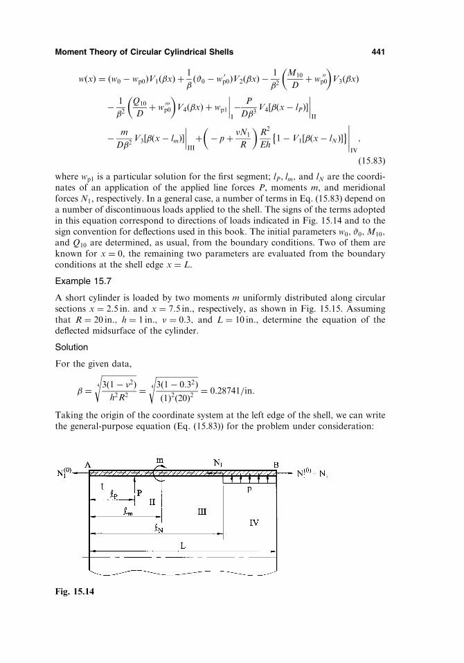
wðxÞ ¼ ðw0 � wp0ÞV1ðxÞ þ1

ð#0 � w 0

p0ÞV2ðxÞ �1

2M10

Dþ wp0

00� �

V3ðxÞ

� 1

2Q10

Dþ wp0

000� �

V4ðxÞ þ wp1

I

� P

D3V4½ðx� lPÞ�

II

� m

D2V3½ðx� lmÞ�

III

þ�� pþ �N1

R

�R2

Eh1� V1½ðx� lNÞ��

IV

;

ð15:83Þwhere wp1 is a particular solution for the first segment; lP; lm; and lN are the coordi-nates of an application of the applied line forces P, moments m, and meridionalforces N1, respectively. In a general case, a number of terms in Eq. (15.83) depend ona number of discontinuous loads applied to the shell. The signs of the terms adoptedin this equation correspond to directions of loads indicated in Fig. 15.14 and to thesign convention for deflections used in this book. The initial parameters w0; #0;M10;and Q10 are determined, as usual, from the boundary conditions. Two of them areknown for x ¼ 0, the remaining two parameters are evaluated from the boundaryconditions at the shell edge x ¼ L.

Example 15.7

A short cylinder is loaded by two moments m uniformly distributed along circularsections x ¼ 2:5 in: and x ¼ 7:5 in:, respectively, as shown in Fig. 15.15. Assumingthat R ¼ 20 in:; h ¼ 1 in:; � ¼ 0:3; and L ¼ 10 in:, determine the equation of thedeflected midsurface of the cylinder.

Solution

For the given data,

¼ffiffiffiffiffiffiffiffiffiffiffiffiffiffiffiffiffiffi3ð1� �2Þh2R2

4

s¼

ffiffiffiffiffiffiffiffiffiffiffiffiffiffiffiffiffiffiffiffiffiffi3ð1� 0:32Þð1Þ2ð20Þ2

4

s¼ 0:28741=in:

Taking the origin of the coordinate system at the left edge of the shell, we can writethe general-purpose equation (Eq. (15.83)) for the problem under consideration:


Fig. 15.14

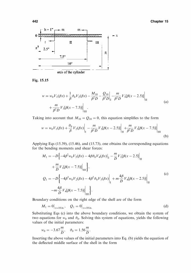
w ¼ w0V1ðxÞ þ1

#0V2ðxÞ �

M10

2D� Q10

3D

I

� m

2DV3½ðx� 2:5Þ�

II

þ m

2DV3½ðx� 7:5Þ�

III

:

ðaÞ

Taking into account that M10 ¼ Q10 ¼ 0, this equation simplifies to the form

w ¼ w0V1ðxÞ þ#0V2ðxÞ

I

� m

2DV3½ðx� 2:5Þ�

II

þ m

2DV3½ðx� 7:5Þ�

III

ðbÞApplying Eqs (15.39), (15.46), and (15.73), one obtains the corresponding equationsfor the bending moments and shear forces:

M1 ¼ �D �42w0V3ðxÞ � 4#0V4ðxÞI�m

DV1½ðx� 2:5�

n II

þm

DV1½ðx� 7:5Þ�

III

�;

Q1 ¼ �D �43w0V2ðxÞ � 42#0V3ðxÞI

þm4

DV4½ðx� 2:5Þ�

II

�m4

DV4½ðx� 7:5Þ�

III

�:

ðcÞ

Boundary conditions on the right edge of the shell are of the form

M1 ¼ 0x¼10 in:

; Q1 ¼ 0x¼10 in:

ðdÞSubstituting Eqs (c) into the above boundary conditions, we obtain the system oftwo equations for w0 and #0. Solving this system of equations, yields the followingvalues of the initial parameters:

w0 ¼ �3:67m

D; #0 ¼ 1:56

m

D:

Inserting the above values of the initial parameters into Eq. (b) yields the equation ofthe deflected middle surface of the shell in the form

442 Chapter 15

Fig. 15.15

tively. As this takes place, the area of an axial cross section for all the three shells isidentical in the interval �c � x � c, i.e., the above shells are of the same weight. Theparallel edges of the shells are simply supported. Assuming that h0 ¼ 0:5; c ¼ 20; R¼ 15; and � ¼ 0:3, determine the deflections, internal forces, and moments in theshell.

Solution

Since the shells and loading are symmetrical about x ¼ 0, all the above problems aresolved for the interval 0 � x � c. Boundary conditions of the simply supported typefor the shell edge x ¼ c and the symmetry conditions for the section x ¼ 0 areprescribed. The numerical values of the components of the state of stress and strainare given in Table 15.1 for h ¼ h1. Analogous results are given in Table 15.2 forh ¼ h2. The system of ordinary differential equations (15.89) was solved byGodunov’s method of discrete orthogonalization. From these tables it is seen howthe thickness redistribution of the shell influences the state of stress and strain underthe condition of the conservation of the shell weight. It makes it possible to select themost efficient parameters of shell structures.


Fig. 15.16

Table 15.1

x ðM1=pÞ 10 ðN1=pÞ 10�1 Q1=p ðw= pEÞ 10�3

0 �0:31633 0.40996 0 0.30976

2 �0:32035 0.40996 �0:39650 10�3 0.31210

4 �0:33230 0.40996 �0:82848 10�3 0.31931

6 �0:35740 0.40996 �1:18812 10�2 0.33193

8 �0:42139 0.40996 �0:50151 10�2 0.35117

10 �0:58015 0.40996 �0:11284 10�1 0.37985

12 �0:86017 0.40996 �0:14980 10�1 0.42531

14 �0:99610 0.40996 �0:97754 10�2 0.50433

16 0:1056 10�1 0.40996 0.10333 0.63605

18 0.29781 0.40996 0.14807 0.71609

20 0 0.40996 �0:73044 0

PROBLEMS

15.1 Indicate cases when the membrane theory alone cannot describe adequately the state of

stress of cylindrical shells under applied transverse loading.

15.2 Verify Eqs (15.21) and (15.24).

15.3 What are the conditions at which a complete state of stress in open and closed cylind-

rical shells can be broken down into elementary states of stress? Characterize these

elementary stress states.

15.4 A long steel pipe is subjected to the edge line load Q0 that is applied uniformly around

the circumference x ¼ 0. The radius and thickness of the pipe are R ¼ 0:5m and

h ¼ 5mm, respectively. (a) Derive and plot the values of w and M vs. x. (b)

Determine the distance x at which the deflections and moments are 5% of their abso-

lute maximum values. Take E ¼ 200GPa; and � ¼ 0:3.15.5 A very long cylinder of radius R and of thickness h is subjected to uniform loading

p0 over L of its length (Fig. 15.11) (a) Determine the ratio of maximum bending

stress to maximum magnitude of membrane stress. (b) Calculate the deflections and

bending moments at a point A for two cases of location of that point, as shown in

Figs 15.11a and b. Take R ¼ 1:5m; h ¼ 6mm; p0 ¼ 5 kPa; E ¼ 200GPa; and

� ¼ 0:3.15.6 Verify Eqs (15.57).

15.7 The infinite circular cylinder of radius R is subjected to a uniformly distributed around

a circumference moment m, as shown in Fig. P.15.1. Assuming that the moment is

applied near the center of the cylinder, find the expressions for w; #;M1; and Q1 as

functions of m and x:15.8 A stiffening ring is placed around a long steel cylindrical shell at a distance remote

from the ends, as shown in Fig. 15.12a. The cylinder is loaded by an internal pressure

p0. Determine stress at the ring attachment if: (a) the ring is assumed to be infinitely

rigid and (b) the ring is assumed to be 100 mm wide and 10 mm thick. Take the radius

of the cylinder as 1.25 m and its thickness as 6 mm, p0 ¼ 10 kPa; E ¼ 200GPa; and� ¼ 0:3:

15.9 Determine stresses in a cylindrical component reinforced by a ring and subjected to

internal pressure p ¼ 4 MPa (Fig. P.15.2). All dimensions in Fig. P.15.2 are given in

mm. Take E ¼ 200GPa; and � ¼ 0:3.

446 Chapter 15

Table 15.2

x M1=p N1=p Q1=p ðw= pEÞ 10�3

0 0:13028 10�4 0:42808 10 0 0.41154

2 0:31492 10�3 0:42808 10 0:29494 10�3 0.41153

4 0:10442 10�2 0:42808 10 0:33756 10�3 0.41140

6 0:82148 10�3 0:42808 10 �0:91417 10�3 0.41095

8 �0:44991 10�2 0:42808 10 �0:48864 10�2 0.41030

10 �0:18990 10�1 0:42808 10 �0:97479 10�2 0.41154

12 �0:27954 10�1 0:42808 10 0:55193 10�2 0.41935

14 0:39696 10�1 0:42808 10 0:73855 10�1 0.43480

16 0.30266 0:42808 10 0.18704 0.43047

18 0.65488 0:42808 10 0:82290 10�1 0.31639

20 0 0:42808 10 �0:97407 0

This example has been taken from Ref. [10]

REFERENCES

1. Gol’denveizer, A.L., Theory of Thin Shells, Pergamon Press, New York, 1961.

2. Novozhilov, V.V., The Theory of Thin Elastic Shells, P. Noordhoff LTS, Groningen, The

Netherlands, 1964.

3. Vlasov, V.X., General Theory of Shells and its Application in Engineering (translated from

Russian), NASA TT F-99, National Aeronautic and Space Administration, Washington,

DC, 1964.

4. Cook, D. and Young, W.C., Advanced Mechanics of Materials, 2nd edn., Prentice Hall,

New Jersey, 1999.

5. Winkler, E., Die Lehre von der Elastizitat und Festigkeit, Prague, 1867.

6. Kreyszig, E., Advanced Engineering Mathematics, 7th edn, John Wiley and Sons, New

York, 1993.

7. Krylov, A.N., On Stresses Experienced by a Ship in a Sea Way, Trans Inst Naval

Architects, London, p. 44, 1902.



9. Collatz, L., The Numerical Treatment of Differential Equations, 3rd edn, Springer-Verlag,

Berlin, 1966.

10. Godunov, S.K., Ordinary Differential Equations with Constant Coefficients (translated

from Russian), Providence, R.I. American Mathematical Society, 1997.

11. Grigorenko, Ia.M. and Mukoed, A.P., The Solution of Problems of the Shell Theory on

Computers, Vushcha Shkola, Kiev, 1979.

448 Chapter 15

Fig. P15.3

16

The Moment Theory of Shells ofRevolution

16.1 INTRODUCTION

As mentioned, shells of revolution belong to a highly general class of shells fre-quently used in engineering. One representative of this class, cylindrical shells, wasconsidered in Chapter 15, and we will not dwell on these shells. The shell typesanalyzed in this chapter are subclasses of shells of revolution having non-zeroGaussian curvature. As mentioned in Sec. 11.7, such shells have non-developablesurfaces. Hence, they are stronger, stiffer, and more stable than shells with zeroGaussian curvature. These shells are frequently used to cover the roofs of sporthalls and large liquid storage tanks. The containment shield structures of nuclearpower plants also have dome-like roofs. Various pressure vessels are either com-pletely composed of a single rotational shell or have shells of revolution at their endcaps. Conical shells with zero Gaussian curvature are also representative of thisclass of shells: they are used to cover liquid storage tanks and the nose cones ofmissiles and rockets.

In the membrane analysis of shells of revolution considered in Chapters 13 and14, we saw that the membrane theory alone cannot accommodate all the loads,support conditions, and geometries in actual shells. Thus, in a general case, shellsof revolution experience both stretching and bending to resist an applied loading,which distinguishes significantly the bending of shells from the elementary behaviorof plates (see also Sec. 10.4).

However, the character of bending deformation may be different. If a shell ofrevolution is subjected to a concentrated force (Fig. 16.1a), bending exerts a crucialeffect on its strength, because, in this case, the bending deformation increases with agrowth of the forces until the load-carrying capacity of the shell structure is exhausted.In places of junction of a shell with its supports (Fig. 16.1b) or other structuralmembers (shell of another geometry, ring beam, etc.), or in places of jump change in

449

the radii of curvature (Fig. 16.1c), the bending has another character; here, bendingpropagates only if it is needed to eliminate the discrepancies between the membranedisplacements or to satisfy the conditions of statics. If a shell material is ductile, thebending deformations of the latter type are usually decreased and do not practicallyinfluence the load-carrying capacity of shell structures. If the material of the shell isbrittle, the bending deformations remain proportional to the applied loads until failureand can result in a significant decrease in the strength of the shell structure

In this chapter we consider the bending theory of shells of revolution. It shouldbe noted that the solutions of the governing differential equations involve manydifficulties for a general shell of revolution, and therefore, we solve these equationsfor some particular shell geometries and load configurations that are frequently usedin engineering practice.

16.2 GOVERNING EQUATIONS

We present below the governing differential equations of the moment theory of shellsof revolution of an arbitrary shape. As curvilinear coordinates and of a point onthe shell middle surface, it is convenient to take the spherical coordinates, introducedin Sec. 11.8, and used in the membrane theory of shells of revolution in Chapters 13and 14. Thus, we take ¼ ’ and ¼ �. As before, the angle ’ defines the location ofa point along the meridian, whereas � characterizes the location of a point along theparallel circle (see Fig. 11.12). Let R1 and R2 be the principal radii of curvature of themeridian and parallel circle, respectively. Obviously, R1 and R2 will be functions of ’only, i.e., R1 ¼ R1ð’Þ and R2 ¼ R2ð’Þ. The Lame parameters in this case are deter-mined by the following formulas (see Sec. 11.8):

A ¼ R1ð’Þ; B ¼ R2ð’Þ sin ’; r ¼ R2 sin ’: ð16:1ÞThe Codazzi and Gauss conditions are given by Eqs (11.41).

Let us consider the kinematic relations of the moment theory of shells ofrevolution. Displacement components of the middle surface along the given coordi-

450 Chapter 16

Fig. 16.1

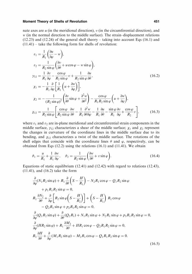
nate axes are u (in the meridional direction), v (in the circumferential direction), andw (in the normal direction to the middle surface). The strain–displacement relations(12.23) and (12.24) of the general shell theory – taking into account Eqs (16.1) and(11.41) – take the following form for shells of revolution:

"1 ¼1

R1

@u

@’� w

� �;

"2 ¼1

R2 sin ’

@v

@�þ u cos ’� w sin ’

� �;

�12 ¼1

R1

@v

@’� cos ’

R2 sin ’vþ 1

R2 sin ’

@u

@�; ð16:2Þ

�1 ¼ � 1

R1

@

@’

1

R1

uþ @w@’

� �� ;

�2 ¼ � 1

R2 sin ’ð Þ2@v

@�sin ’þ @

2w

@�2

!� cos ’

R1R2 sin ’uþ @w

@’

� �;

�12 ¼1

R2 sin ’

cos ’

R2 sin ’

@w

@�� 1

R1

@2w

@�@’� 1

R1

@u

@�� sin ’

R1

@v

@’þ cos ’

R2

v

" #; ð16:3Þ

where "1 and "2 are in-plane meridional and circumferential strain components in themiddle surface, �12 characterizes a shear of the middle surface; �1 and �2 representthe changes in curvature of the coordinate lines in the middle surface due to itsbending, and �12 characterizes a twist of the middle surface. The rotations of theshell edges that coincide with the coordinate lines � and ’, respectively, can beobtained from Eqs (12.2) using the relations (16.1) and (11.41). We obtain

#1 ¼u

R1

þ 1

R1

@w

@’; #2 ¼

1

R2 sin ’

@w

@�þ v sin ’

� �: ð16:4Þ

Equations of static equilibrium (12.41) and (12.42) with regard to relations (12.43),(11.41), and (16.2) take the form

@

@’N1R2 sin ’ð Þ þ R1

@

@�S � H

R1

� ��N2R1 cos ’�Q1R2 sin ’

þ p1R1R2 sin ’ ¼ 0;

R1

@N2

@�þ @

@’R2 sin ’ S � H

R2

� �� þ S � H

R1

� �R1 cos ’

�Q2R1 sin ’þ p2R1R2 sin ’ ¼ 0;

@

@’ðQ1R2 sin ’Þ þ

@

@�ðQ2R1Þ þN1R2 sin ’þN2R1 sin ’þ p3R1R2 sin ’ ¼ 0;

@

@’ðHR2 sin ’Þ þ R1

@M2

@�þHR1 cos ’�Q2R1R2 sin ’ ¼ 0;

R1

@H

@�þ @

@’ðM1R2 sin ’Þ �M2R1 cos ’�Q1R1R2 sin ’ ¼ 0:

ð16:5Þ

Moment Theory of Shells of Revolution 451

Kinematic equations (strain–displacement relations)

"1k ¼1

R1

dukd’

� wk

� �;

"2k ¼1

R2 sin ’ðkvk þ uk cos ’� wk sin ’Þ;

�12k ¼1

R1

dvkd’

� cos ’

R2 sin ’vk �

kukR2 sin ’

;

�1k ¼ � 1

R1

d

d’

ukR1

þ 1

R1

dwk

d’

� �;

�2k ¼ � 1

ðR2 sin ’Þ2kvk sin ’� k2wk

� �� cos ’

R1R2 sin ’uk þ

dwk

d’

� �;

�12k ¼1

R2 sin ’� cos ’

R2 sin ’kwk þ

k

R1

dwk

d’þ k

R1

uk �sin ’

R1

dvkd’

þ cos ’

R2

vk

� �;

#1k ¼1

R1

uk þdwk

d’

� �; #2k ¼

1

R2 sin ’ð�kwk þ vk sin ’Þ

ð16:8ÞEquations of static equilibrium

d

d’N1kR2 sin ’ð Þ þ R1kSk �

1

R1

d

d’ðM1kR2 sin ’Þ þM2k cos ’

� 2kHk �N2kR1 cos ’þ p1kR1R2 sin ’ ¼ 0

� R1kN2k þ1

R2 sin ’

d

d’SkðR2 sin ’Þ2� �

� 1

R2

R1ð�kÞM2k þ 2R2 sin ’dHk

d’

�þ2 cos ’HkðR1 þ R2Þ

�

þ p2kR1R2 sin ’ ¼ 0:

N1k

R1

þN2k

R2

þ 1

R1R2 sin ’

d

d’

Hkkþ 1

R1

d

d’ðM1kR2 sin ’Þ �M2k cos ’

� �

þ 1

R2 sin ’

k

R2 sin ’

d

d’ðR2 sin ’Þ2Hk

� �� k2R1M2k

� ��þ p3k ¼ 0:

ð16:9Þ

Equations (16.8) and (16.9), together with the constitutive equations (12.45) and(12.46) and proper boundary conditions, form the closed eight-order system of theordinary differential equations for each kth harmonic of the expansion (16.7). Thissystem of the governing equations describes the state of stress and strain for thegeneral moment theory of shells of revolution having a meridian of an arbitraryshape. This system of ordinary equations may be solved by applying the standardnumerical methods intended for a solution of ordinary differential equations andintroduced, for example, in Refs. [1,2]. The finite element method can also be appliedto the analysis of the state of stress and strain for shells of revolution of a generalshape [3,4].


N1 ¼ B1

R1

du

d’� w

� �þ �

R2

ðu cot ’� wÞ� �

; ð16:15aÞ

N2 ¼ B1

R2

ðu cot ’� wÞ þ �

R1

du

d’� w

� �� ; ð16:15bÞ

M1 ¼ �D1

R1

d#1d’

þ �

R2

#1 cot ’

� �; ð16:15cÞ

M2 ¼ �D1

R2

#1 cot ’þ�

R1

d#1d’

� �; ð16:15dÞ

where

B ¼ Eh

1� �2 ;D ¼ Eh3

12ð1� �2Þ : ð16:16Þ

Equations (16.11), (16.12), and (16.13) or (16.15) form a closed system of 12ordinary differential equations for 12 unknowns (strains, stress resultants andcouples). Solving this system of equations, one obtains the internal forces, moments,and displacements. The stress components are calculated by the following formulas:

�1max ¼N1

hþ 6M1

h2; �2max ¼

N2

hþ 6M2

h2: ð16:17Þ

Let us bring the above system of equations to two symmetric governing equa-tions for two unknowns. Following Meissner [5], we introduce the new variables

#1 and U ¼ R2Q1ð’Þ: ð16:18ÞWe now express the internal forces and moments in terms of the new variables.Canceling the circumferential force N2 from the first and second Eqs (16.12), weobtain the following equation:

1

R1

d

d’ðN1 sin ’þQ1 cos ’Þr½ � þ ðp1 sin ’þ p3 cos ’Þr ¼ 0: ð16:19Þ

Integrating this equation over ’, we obtain

ðN1 sin ’þQ1 cos ’Þr ¼ �Fð’Þ; ð16:20Þwhere

Fð’Þ ¼ð’’e

R1rðp1 sin �’’þ p3 cos �’’Þd �’’þ C; ð16:21Þ

here �’’ is a dummy variable; ’e is the angular coordinate of one of the shell edges –say, the top edge; Fð’Þ represents the resultant of all external surface loads applied toan isolated part of the shell per unit ’; and C takes into account an axial componentof the external loads applied to the top edge of the shell.

Comparing Eqs (16.21) and (13.37), we can conclude that a particular solutionof Eq. (16.19), corresponding to the integral Fð’Þ; represents a membrane solution ofthe general bending theory of axisymmetrically loaded shells of revolution.

Taking into account Eq. (16.18), we can express the meridional force N1 interms of U from Eq. (16.20), as follows:


#1e ¼ �Me

DR1 þ

QeR21

22D;

N1e ¼ �Qe cot ’e;N2e ¼ Me

2R22

R21

�Qe

2R2

R1

;

"2e ¼1

EhMe

2R22

R21

�Qe

2R2

R1

þ �Qe cot ’e

" #; �e ¼ "2ere ¼ "2eR2e sin ’e:

ð16:51ÞThe upper signs in all the above equations refer to the top edge of the shell, whereasthe lower signs refer to the bottom edge. If a shell of revolution is loaded by thehorizontal force (thrust) He per unit length applied to the shell edge ’ ¼ ’e, then theinternal forces and deformations can also be determined from Eqs (16.50) and(16.51) by substituting for Qe from the following equation:

Qe ¼ �He sin ’e: ð16:52ÞIf an arbitrary surface load is applied to the shell of revolution, then the solutions(16.48) must be complemented by a particular solution of the nonhomogeneousequations. This particular solution in most cases is determined from the membranetheory of shells introduced in Chapter 13 .

The accuracy of the introduced approximate Geckeler’s analysis was analyzedin Refs [5–9]. It has been established that for thin shells with fairly big angle of rise,these formulas give satisfactory accurate results. The error of approximate formulasof the edge effect theory has an order of

ffiffiffiffiffiffiffiffiffiffiffiffiffiffiffiffiffiffiffiffiffih cot2 ’=R

p. Practically, this method can be

used if the angle of the shell edge ’e > 35.In the next section we apply the approximate solution procedure discussed

above to the analysis of some specific geometric forms of shells of revolution usedin practical application. We assume that for the geometry of the shells under con-sideration all requirements about accuracy of applicability of the approximatemethod introduced above are satisfied.

16.5 AXISYMMETRIC SPHERICAL SHELLS, ANALYSIS OF THESTATE OF STRESS AT THE SPHERICAL-TO-CYLINDRICALJUNCTION

For spherical shells, R1 ¼ R2 ¼ R, and the governing equations of axisymmetricbending of shells of revolution, Eqs (16.40) are simplified. The solution procedurebased on the approximate method introduced in Sec. 16.4, as applied to the bendinganalysis of axisymmetrically loaded spherical shells, is illustrated below by the fol-lowing examples.

Example 16.1

Calculate stresses in the hemispherical shell stiffened on its edge by a flange andloaded by an internal pressure p which is balanced by a force P, as shown in Fig.16.6a. Given R ¼ 50 cm; h ¼ 0:3 cm; r1 ¼ 49:85 cm; r2 ¼ 53 cm; r3 ¼ 51:6 cm; b ¼3:15 cm; h1 ¼ 0:8 cm; � ¼ 0:3, and E ¼ 20GPa.

464 Chapter 16

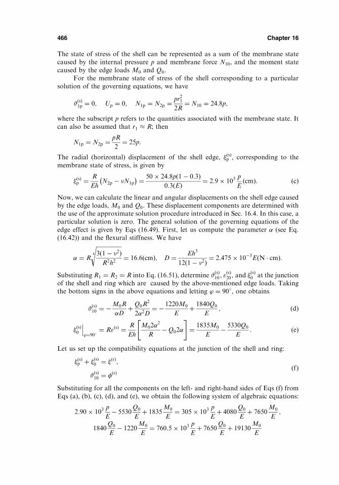
The state of stress of the shell can be represented as a sum of the membrane statecaused by the internal pressure p and membrane force N10, and the moment statecaused by the edge loads M0 and Q0.

For the membrane state of stress of the shell corresponding to a particularsolution of the governing equations, we have

#ðsÞ1p ¼ 0; Up ¼ 0; N1p ¼ N2p ¼ pr212R

¼ N10 ¼ 24:8p;

where the subscript p refers to the quantities associated with the membrane state. Itcan also be assumed that r1 � R; then

N1p ¼ N2p ¼ pR

2¼ 25p:

The radial (horizontal) displacement of the shell edge, �ðsÞp , corresponding to themembrane state of stress, is given by

�ðsÞp ¼ R

EhN2p � �N1p

� � ¼ 50 24:8pð1� 0:3Þ0:3ðEÞ ¼ 2:9 103

p

EðcmÞ: ðcÞ

Now, we can calculate the linear and angular displacements on the shell edge causedby the edge loads, M0 and Q0. These displacement components are determined withthe use of the approximate solution procedure introduced in Sec. 16.4. In this case, aparticular solution is zero. The general solution of the governing equations of theedge effect is given by Eqs (16.49). First, let us compute the parameter (see Eq.(16.42)) and the flexural stiffness. We have

¼ R

ffiffiffiffiffiffiffiffiffiffiffiffiffiffiffiffiffiffi3ð1� �2ÞR2h2

4

s¼ 16:6ðcmÞ; D ¼ Eh3

12ð1� �2Þ ¼ 2:475 10�3EðN � cmÞ:

Substituting R1 ¼ R2 ¼ R into Eq. (16.51), determine #ðsÞ10; "ðsÞ20; and �

ðsÞ0 at the junction

of the shell and ring which are caused by the above-mentioned edge loads. Takingthe bottom signs in the above equations and letting ’ ¼ 90, one obtains

#ðsÞ10 ¼ �M0R

DþQ0R

2

22D¼ � 1220M0

Eþ 1840Q0

E; ðdÞ

�ðsÞ0’¼90

¼ R"ðsÞ ¼ R

Eh

M022

R�Q02

" #¼ 1835M0

E� 5330Q0

E: ðeÞ

Let us set up the compatibility equations at the junction of the shell and ring:

�ðsÞp þ �ðsÞ0 ¼ �ðrÞ;

#ðsÞ10 ¼ �ðrÞðfÞ

Substituting for all the components on the left- and right-hand sides of Eqs (f) fromEqs (a), (b), (c), (d), and (e), we obtain the following system of algebraic equations:

2:90 103p

E� 5530

Q0

Eþ 1835

M0

E¼ 305 103

p

Eþ 4080

Q0

Eþ 7650

M0

E;

1840Q0

E� 1220

M0

E¼ 760:5 103

p

Eþ 7650

Q0

Eþ 19130

M0

E

466 Chapter 16

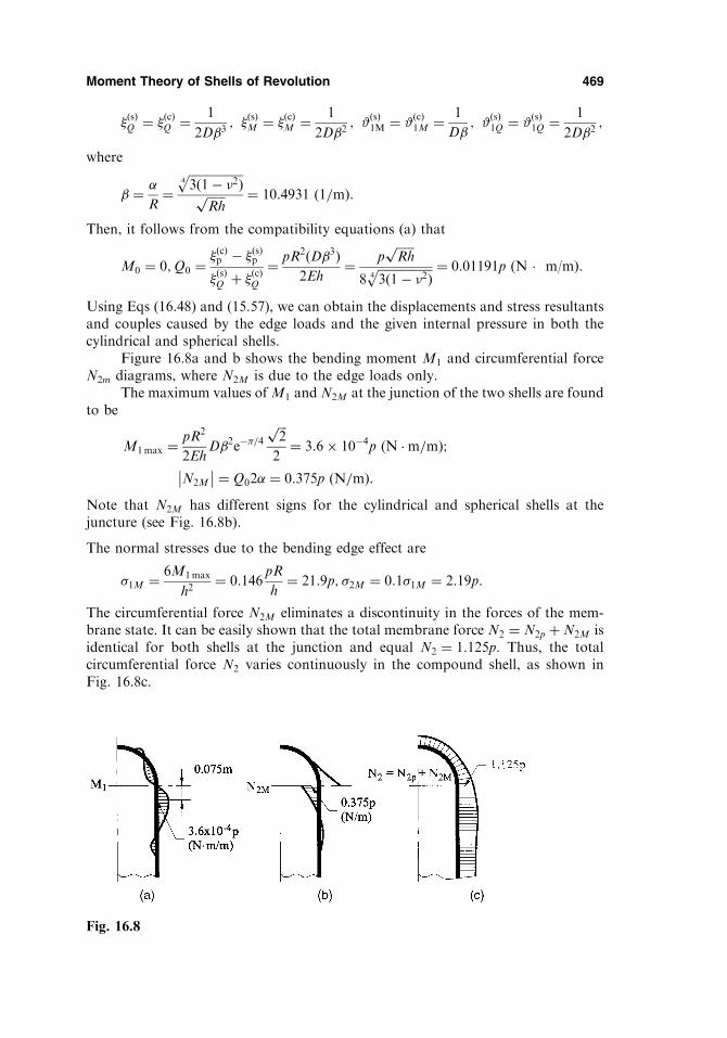
�ðsÞQ ¼ �ðcÞQ ¼ 1

2D3; �ðsÞM ¼ �ðcÞM ¼ 1

2D2; #ðsÞ1M ¼ #ðcÞ1M ¼ 1

D; #ðsÞ1Q ¼ #ðsÞ1Q ¼ 1

2D2;

where

¼

R¼

ffiffiffiffiffiffiffiffiffiffiffiffiffiffiffiffiffiffi3ð1� �2Þ4

pffiffiffiffiffiffiRh

p ¼ 10:4931 ð1=mÞ:

Then, it follows from the compatibility equations (a) that

M0 ¼ 0;Q0 ¼�ðcÞp � �ðsÞp�ðsÞQ þ �ðcÞQ

¼ pR2ðD3Þ2Eh

¼ pffiffiffiffiffiffiRh

p

8ffiffiffiffiffiffiffiffiffiffiffiffiffiffiffiffiffiffi3ð1� �2Þ4

p ¼ 0:01191p (N � m/m).

Using Eqs (16.48) and (15.57), we can obtain the displacements and stress resultantsand couples caused by the edge loads and the given internal pressure in both thecylindrical and spherical shells.

Figure 16.8a and b shows the bending moment M1 and circumferential forceN2m diagrams, where N2M is due to the edge loads only.

The maximum values ofM1 and N2M at the junction of the two shells are foundto be

M1max ¼pR2

2EhD2e��=4

ffiffiffi2

p

2¼ 3:6 10�4p ðN �m=mÞ;

N2M

¼ Q02 ¼ 0:375p ðN=mÞ:Note that N2M has different signs for the cylindrical and spherical shells at thejuncture (see Fig. 16.8b).

The normal stresses due to the bending edge effect are

�1M ¼ 6M1max

h2¼ 0:146

pR

h¼ 21:9p; �2M ¼ 0:1�1M ¼ 2:19p:

The circumferential force N2M eliminates a discontinuity in the forces of the mem-brane state. It can be easily shown that the total membrane force N2 ¼ N2p þN2M isidentical for both shells at the junction and equal N2 ¼ 1:125p. Thus, the totalcircumferential force N2 varies continuously in the compound shell, as shown inFig. 16.8c.


Fig. 16.8

It is seen that the stresses due to the edge effect have a magnitude of the sameorder ðpR=hÞ as the membrane stresses in the shells under consideration. This istypical for shells at which the edge effect occurs, because the compatibility of defor-mations is not satisfied by the membrane state only.

Example 16.3

A compound steel shell consists of a cylinder (radius R and wall thickness h) and of ahead in the form of a spherical segment (radius Rs ¼ 2R and thickness h), as shownin Fig. 16.9a. This compound shell is subjected to an internal pressure p. Determinethe internal forces and moments in the compound shell if R ¼ 1:5m; h ¼ 0:02m; � ¼0:3; E ¼ 200GPa, and ’1 ¼ 30.

Solution

First, consider the membrane state of the head and cylinder separately, as shown inFig. 16.9b. From the membrane shell theory, it follows that

NðsÞ1p ¼ N

ðsÞ2p ¼ pRs

2¼ pR; N

ðcÞ1p ¼ pR

2;NðcÞ

2p ¼ pR ðaÞ

where, again, the subscript p refers to the membrane solution and superscripts s andc stand for the sphere and cylinder, respectively. It is seen from Fig. 16.9b that, apartfrom the latter example, the membrane state alone does not satisfy the conditions ofstatic equilibrium in the head and cylinder. Therefore, the edge effect occurs at thejunction of the compound shell to satisfy both the statics and compatibility ofdeformations conditions.

Consider the edge effect procedure being applied to the given compound shell.The membrane force N

ðsÞ1p at the edge of the head has a horizontal component, which

is equal to

470 Chapter 16

Fig. 16.9

T0 ¼ NðsÞ1p cos ’1 ¼ pR

ffiffiffi3

p

2: ðbÞ

To ensure that the shell loading by the membrane scheme (Fig. 16.9b), together withthe edge effect, would be equivalent to the given loading applied to the compoundshell, it is necessary to include the thrust that is equal and oppositely directed to T0

among the edge effect forces, as shown in Fig. 16.8c. Thus, in applying the edgeeffect solution procedure, we should assume that the cylindrical shell is loaded by theedge moment M0 and shear force H0, whereas the spherical shell is loaded by theedge moment M0 and thrust ðH0 � T0Þ, as shown in Fig. 16.9c. The unknown quan-tities M0 and H0 are evaluated from the compatibility of deformations’ conditions,i.e., the radial (horizontal) displacements and angles of rotation of normals shouldbe identical at the juncture of both shells. Equating the edge radial displacements ofthe sphere and cylinder at the juncture, we obtain

�ðsÞ ¼ �ðcÞ ðcÞ

where,

�ðsÞ ¼ � R

EhðNðsÞ

2p � �NðsÞ1p Þ þ ðT0 �H0Þ�ðsÞH �M0�

ðsÞM

�ðcÞ ¼ � R

EhN

ðcÞ2p � �NðcÞ

1p Þ þH0�ðcÞH �M0�

ðcÞM :

� ðdÞ

In Eqs (c) and (d), the first terms on the right-hand sides correspond to the mem-brane solution.

The conditions of compatibility for the slopes (the positive direction of theslopes is shown in Fig. 16.9c to the right) has the form

ðT0 �H0Þ#ðsÞ1H �M0#ðsÞ1M ¼ �H0#

ðcÞ1H þM0#

ðcÞ1M : ðeÞ

In Eqs. (d) and (e), the subscripts H and M indicate the cause of the correspondingdisplacements. The coefficients �ðsÞH ; �

ðsÞM ; #

ðsÞ1H; #

ðsÞM and �ðcÞH ; �

ðcÞM ; #

ðcÞ1H; #

ðcÞ1M can be

calculated from Eqs (16.51) by setting R1 ¼ R2 ¼ Rs ¼ 2R; ’e ¼ ’1; and replacingQ0 with H0 sin ’1 or T0 sin ’1) according to Eq. (16.50) for the spherical shell, andby setting R1 ¼ 1; R2 ¼ R; and ’e ¼ ’1 for the cylindrical shell. As a result, weobtain

�ðsÞH ¼ sin2 ’12D3s

; �ðsÞM ¼ sin ’12D2s

; #ðsÞ1M ¼ 1

Ds; #ðsÞ1H ¼ �ðsÞM ;

�ðcÞH ¼ 1

2D3c; �ðcÞM ¼ 1

2D2c; #ðcÞM ¼ 1

Dc; #ðcÞ1H ¼ �ðcÞM ;

s ¼ffiffiffiffiffiffiffiffiffiffiffiffiffiffiffiffiffiffi3ð1� �2Þ4

pffiffiffiffiffiffiffiffiffi2Rh

p ; c ¼ffiffiffiffiffiffiffiffiffiffiffiffiffiffiffiffiffiffi3ð1� �2Þ4

pffiffiffiffiffiffiRh

p :

ðfÞ


Substituting the numerical data into the relations (a), (b), (d), and (f), one obtains thefollowing:

D ¼ Eh3

12ð1� �2Þ ¼ 146:52 103ðNmÞ; c ¼ 7:4213ð1=mÞ; s ¼ 5:2477ð1=mÞ;

NðsÞ1p ¼ N

ðsÞ2p ¼ 1:5p ðN=mÞ; N

ðcÞ1p ¼ 0:75p ðN=mÞ; N

ðcÞ2p ¼ 1:5p; T0 ¼ 1:3p ðN=mÞ;

�ðsÞH ¼ 0:005903 10�6ðm2=NÞ; �ðsÞM ¼ 0:06196 10�6ðm=NÞ;#ðsÞM ¼ 1:301 10�6ð1=NÞ;

�ðcÞH ¼ 0:008362 10�6ðm2=NÞ; �ðcÞM ¼ 0:06196 10�6ðm=NÞ;#ðcÞM ¼ 0:9196 10�6ð1=NÞ:

Substituting the above into the compatibility equations (c) and (e) and taking intoaccount the relations (d), we can calculate H0 and M0. We have

H0 ¼ 0:5401p ðN=mÞ; M0 ¼ 0:03627p ðN �m=mÞ:Using Eqs (16.48) for a spherical shell and Eqs (15.57) for the cylindrical shell, wecan determine the membrane forces N2;N1 and bending moments M1;M2 in thespherical and cylindrical parts of the given compound shell. The equations for themembrane forces and bending moments are of the following form:

– for the cylindrical shell

NðcÞ2 ¼ 1:5p 1� 4:0075e�cxðcoscxþ sin cxÞ

� �; N

ðcÞ1 ¼ 0:75p;

MðcÞ1 ¼ 0:03627pe�cxðcoscx� sin cxÞ;

ðgÞ

where the coordinate x is counted off from the juncture of the spherical and cylind-rical shells.–for the spherical shell

NðsÞ2 ¼ 1:5p 1� 4:0075e�!ðcos!þ sin !Þ½ �;

NðsÞ1 ¼ 1:5p 1� 0:44e�! cos!½ �;

MðsÞ1 ¼ 0:03627pe�!ðcos!� sin !Þ;

ðhÞ

where ¼ Rss and ! ¼ ’1 � ’ ¼ 30 � ’.The diagrams of the membrane force N2 and bending momentM1 are shown in

Fig. 16.10.The maximum normal stresses occur in the cylindrical shell at points in its

inner surface at the junction with the sphere segment. The total meridional stressis tensile at the above points and is equals to

�1 ¼N1

hþ 6M1

h2¼ 37:5pþ 544p ¼ 581:5p: ðiÞ

The circumferential stress at the same points is compressive and is given by

�2 ¼N2

hþ � 6M1

h2¼ �61:8p: ðjÞ

472 Chapter 16

It can be shown that in the given compound shell the edge effect normal stress islarger by an order of magnitude

ffiffiffiffiffiffiffiffiffiffiffiffiðR=hÞpthan the corresponding membrane stress.

Therefore, the compound shell, like that analyzed in this example, is inefficient.However, it is possible to essentially decrease the stresses at the junction of

compound shell structures. Figure 16.11a shows two shells, cylindrical and spherical,joined by a ring. The latter is supposed to support the thrust T0 (Fig. (16.11a)). In theanalysis of such shell structures, one can assume that the bending stiffness of the ringin the direction perpendicular to its plane is negligible. Thus, the ring resists only theradial load in its own plane. The free-body diagrams of the shells and ring are shownin Fig. 16.11b.

Let us determine the stress components at the junction of the two shells, shownin Fig. 16.11. The geometrical and mechanical parameters of the shells are takenfrom Example 16.3.

The values of the unknown interface forces, H1 and H2, as well the momentM0, are evaluated from the conditions of deformations, compatibility of the shellparts and ring. Let the shell and ring be made of the same material. Assume that the


Fig. 16.10

Fig. 16.11

Comparing this bending stress due to the edge effect with the corresponding stressfrom the previous example, we can conclude that the setup of the ring allows one todecrease the edge effect maximum stress by more than two times, although the abovestress remains quite considerable.

16.6 AXISYMMETRICALLY LOADED CONICAL SHELLS

For a conical shell, a distance s measured from the vertex of the cone along thestraight meridian may be conveniently taken as a meridional coordinate of a pointon the middle surface (see Sec. 13.6.2). Replacing the variable ’ with a new variables, we use the following obvious relationships

ds ¼ R1d’;dð. . .Þd’

¼ R1

dð. . .Þds

ð16:53aÞ

For conical shells R1 is a constant at infinity and does not vary with s, so thatdR1=ds ¼ 0; hence,

d2ð. . .Þd’2

¼ R21

d2ð. . .Þds2

and R2 ¼ s cot ’;dR2

ds¼ cot ’: ð16:53bÞ

where ’ is the constant value for all points on the straight meridian (Fig. 13.3).In this section, we are concerned with the bending theory of a conical shell

subjected to axisymmetrically applied edge loads. Therefore, we seek only solutionsof the homogeneous bending theory equations (the edge effect solutions), becausethe membrane solution may be used as a particular integral of the general theoryequations for conical shells. Using the relationships (16.53), we can rewrite thegoverning equation (16.28) in terms of the variable s, setting R1 ¼ 1 for conicalshells and �ð’Þ ¼ 0, as follows:

d2#1ds2

þ 1

s

d#1ds

� 1

s2#1 ¼ � 1

DR2

U;

d2U

ds2þ 1

s

dU

ds� 1

s2U ¼ Eh

R2

#1;

ð16:54aÞ

or in the following operator form

L1ð#1Þ þ1

DU ¼ 0

L1ðUÞ � Eh#1 ¼ 0

ð16:54bÞ

where the operator L1ð::Þ is given by

L1ð. . .Þ � cot ’ sd2ð. . .Þds2

þ dð. . .Þds

� 1

sð. . .Þ

" #:

The solution of the governing differential equations (16.54b) can be expressed interms of the Bessel functions or their modifications [13]. However, this rigorousapproach is not suited to practical engineering calculations, as it is too lengthyeven when tables of the Bessel functions are available. The problem of strainingthe conical shells may be solved by using the numerical methods introduced inChapter 6 or by the finite element method technique [3,4].


A simpler solution for the conical shell problems, analogous to the Geckelerapproximation, (see Sec. 16.4) is now introduced. Dropping terms with #1 andd#1=ds and the terms U and dU=ds from the left-hand sides of Eqs (16.54a), yieldsthe following approximate equations:

d2#1ds2

� � U

DR2

;

d2U

ds2� Eh

R2

#1:

ð16:55Þ

Differentiating the second equation twice with respect to s and substituting it into thefirst equation, gives the following governing differential equation of the edge effectfor conical shells:

d4U

ds4þ Eh

R22D

U ¼ 0 or

d4U

ds4þ 44U ¼ 0;

ð16:56Þ

where

¼ffiffiffiffiffiffiffiffiffiffiffiffiffiffiffiffiffiffi3ð1� �2ÞR2

2h2

4

s: ð16:57Þ

Remember that in deriving the governing differential equation of the edge effectthe following assumptions have been adopted: the lower derivatives of functionsand functions themselves are small compared with the higher derivatives and theradius R2 varies slightly near the shell edge. It has been shown that these assump-tions are fairly fulfilled if

ffiffiffiffiffiffiffiffiffiffiffiffiffiffiffiffiffiffiffiffih=ðr sin ’Þp � 1 (r is the radius of the parallel circle)

[14] or for conical shells with a considerable slope of the meridian(’ > 35 � 40).

Let x be the coordinate measured from the edge of interest. Then we have

– for the top edge x ¼ s� s0,– for the bottom edge x ¼ s0 � s,

where s0 is some coordinate that corresponds to the given edge of the shell. Intransition to the variable x, Eq. (16.56) remains unchanged, i.e.,

d4U

dx4þ 44U ¼ 0: ð16:58Þ

Using the edge effect procedure, developed in Sec. 16.4, we can obtain thesolution of Eq. (16.58) and the following expressions for the deformations, internalforces, and moments in a conical shell subjected to the edge loadsMe and Qe in termsof the variable x, as follows:

476 Chapter 16

Using Eqs (16.59) and setting x ¼ 0, we can calculate the angle of rotation of thenormal to the meridian, #1, and the internal forces at the bottom edge. We have

#1 ¼ � m

Dþ Qe

22D¼ �2:29

m

Dþ 2:28

H

D;

N1 ¼ �Qe cot ’ ¼ �0:5H;

N2 ¼ 2R2ðm�QeÞ ¼ 6:58m� 13:1H:

Comparing these numerical data with those obtained by using the exact edge effectprocedure based on the use of the Bessel functions [12], we can conclude that theerror of this approximate analysis does not exceed 1% for the given case.

16.7 AXISYMMETRIC DEFORMATION OF TOROIDAL SHELLS

Structural components having a form of toroidal shells are commonly used inmechanical engineering. Housings of pumps, hydraulic clutches, tanks, bellows,etc., are examples of such shape of a shell. The shape of a toroidal shell is character-ized by the radii R and a and by the following parameters (Fig.16.14):

478 Chapter 16

Fig. 16.13

Fig. 16.14

¼ a

R; ¼ a

h: ð16:60Þ

For a toroidal shell, the principal radii of curvature are (Fig. 16.13)

O1A ¼ R1 ¼ a ¼ const; O2A ¼ R2 ¼ R1þ sin ’

sin ’; ð16:61Þ

where ’ is the angular coordinate varying in the range �180 < ’ < 180. Toroidalshells, except for shallow part near ’ ¼ 0, can be successfully analyzed by the meth-ods of the theory of edge effect (see Sec. 16.4).

For shells including the shallow part near ’ ¼ 0, the problem becomes morecomplicated. Considerable difficulties are associated with determining a particularsolution of the nonhomogeneous governing differential equations, because the mem-brane solution near ’ ¼ 0 becomes invalid. Thus, toroidal shells must be analyzed byusing the governing equations of the general moment theory of axisymmetric shellsof revolution. Substituting for the principal radii of curvature from the relations(16.61) into Eqs (16.30), we obtain the following governing differential equations ofthe axisymmetric deformation of toroidal shells:

L2ðUÞ þ �L2ðUÞ ¼ Eha#1ð’Þ þ� ð’Þ;

L2ð#1Þ � �#1 ¼ � a

DU;

ð16:62Þ

where

L2ð. . .Þ ¼1þ sin ’

sin ’

d2ð. . .Þd’2

þ cot ’dð. . .Þd’

� cot ’ cos ’1þ sin ’ ð. . .Þ;

� ð’Þ ¼ a2d

d’p3

1þ sin ’ð Þ22 sin2 ’

" #þ p1a

2 ð1þ sin ’Þ sin ’

1þ sin ’ sin ’

þ ��

þ Fð’Þ cos ’ð2þ 3 sin ’Þ sin4 ’ð1þ sin ’Þ :

ð16:63ÞThe solution of Eqs (16.62) can be obtained by numerical methods introduced inChapter 6 – in particular, by the finite element method.

PROBLEMS

16.1 Derive Eqs (16.5).

16.2 Derive Eqs (16.9).

16.3 Show that the vertical displacement of a point in the middle surface of shell of revolu-

tion, (see Fig. 16.1) are governed by the following equation

¼ð’’0

ð"1 sin �’’þ #1 cos �’’ÞR1d �’’:

16.4 Verify Eqs (16.50).

16.5 Consider a spherical dome supporting its own weight and described in Sec. 14.1.1.

Assume that the supports are as shown in Fig. 14.2a. (a) Determine the bending

stresses and (b) compare the bending and membrane stresses. Assume reasonable

values for any additional properties and parameters required.


16.6 A dome in the form of a spherical segment is clamped around its base and is loaded by

an external pressure p ¼ 1:5 MPa. Determine the force and moment applied to the base

of the shell by support. Take ’1 (the meridional angle at the shell base)=55, E ¼200GPa; � ¼ 0:3; h ¼ 20 mm, and R ¼ 1500 mm.

16.7 A cylindrical tank is capped by a hemispherical shell, as shown in Fig. 16.6. The tank is

loaded by an internal pressure p ¼ 1:4 MPa. Determine the discontinuity stresses at the

junction. Take the allowable membrane stress �all ¼ 120 Mpa, E ¼ 200GPa � ¼ 0:3,R ¼ 1000mm, hc ¼ hs ¼ 12mm, where hc and hs are the thicknesses of the cylindrical

tank and hemispherical shell, respectively.

16.8 A hemispherical cap of radius R and thickness h is loaded by uniformly applied to the

free edge of the cap moments M0. Determine the length L, measured along the mer-

idian from the loaded edge of the cap, where the internal momentM1 diminishes to 1%

of moment M0. How does this length compare with that in Example 15.1 for a cylind-

rical shell?

16.9 Redo Problem 16.8 replacing the moments M0 with uniformly applied horizontal

forces Q0 to the free edge of the cap.

16.10 What is the maximum stress at the junction of the flat circular plate and (a) hemi-

spherical shell (Fig. P.16.1a) and (b) conical shell with ¼ 37 (Fig. P.16.1b)? Both

shells are subject to an internal pressure of p ¼ 1:5 MPa. Let E ¼ 200GPa; and

� ¼ 0:27.16.11 A conical frustum has a free edge at its top and it is built-in at the base. The shell is

subject to internal pressure p. Determine the internal forces and bending moments in

the shell. Let the radii of the parallel circles at the shell top and its base be 5.5 m and

8.5m, respectively, h ¼ 60mm; E ¼ 200GPa; and � ¼ 0:3. Employ the approximate

method of Sec. 16.4 to determine the bending stress resultants and couples.

16.12 Calculate the displacements of the edge of the hemispherical shell shown in Fig. 16.5a.

For your calculations use the numerical data in Example 16.1.

16.13 Compare the values of the normal stresses in the spherical shell segment for four

variants of boundary conditions at its base: (a) the shell is loaded by a normal mer-

idional force Ne applied to its free edge; (b) the shell is built-in; (c) the shell has roller

supports at its free edge; and (d) the shell is simply supported. The shell is subjected to

an external normal pressure p. Let R ¼ 30h and ’1 ¼ 35(meridional angle at the shell

base) for all the above-mentioned shells. Employ the approximate method of Sec. 16.4

for the solution.

16.14 Consider the Intze-type water tank of Problem 14.18 (Fig. 14.14a). (a) Find the bend-

ing stress resultants and couples in the wall and the roof and plot their diagrams.

(b) Assume that there is no ring beam at B. Find the final value of N2 in the cone

at B using the moment theory. Neglect the effects of discontinuities at C on the stresses

480 Chapter 16

Fig. P16.1

17

Approximate Theories of ShellAnalysis and Their Applications

17.1 INTRODUCTION

The complexity of the governing equations of the general linear theory of thin shellsmotivated the development of a wide range of approximate theories associated withsimplifications of these equations.

There are two principal avenues in developing these approximate theories. Thefirst avenue is based on introducing some additional hypotheses (except for thegeneral Kirchhoff–Love assumptions) that follow from the mechanical analysis ofshell straining under applied loading, numerical results of solving various particularshell problems, and from experimental investigations [1–4, etc.]. The second avenueis based on the asymptotic analysis of the governing differential equations of thegeneral linear theory of thin shells having a small parameter a (see Sec. 15.2) [5].Both avenues arrive at the same results. However, the second avenue provides a wayfor an error estimation of the corresponding approximate equations. Note that thepossibility of introducing one or other simplification is determined by the characterof loading (its variation), boundary conditions, and the shell stiffness and its othergeometric parameters.

In this chapter we consider only the first avenue of simplifications and thecorresponding approximate theories.

17.2 THE SEMI-MEMBRANE THEORY OF CYLINDRICAL SHELLS

In the analysis of long closed and open cylindrical shells, the so-called semi-mem-brane theory has enabled a wide range of applications. It enables one to analyze theabove-mentioned shells with the use of simple (and well-known for engineers) math-ematical technique in situations when the membrane theory is not applicable.

483

EhX1k¼1

d4Vk

dx4þ h2

12R6Vkk

4ðk2 � 1Þ2" #

sin k� ¼X1k¼1

Pk sin k�: ð17:20aÞ

The above results in the following system of ordinary differential equations of thefollowing type:

d4V1

dx4¼ 1

EhP1;

d4V2

dx4þ h2

12R624ð22 � 1Þ2V2 ¼

1

EhP2;

. . . . . . . . . . . . . . . . . . . . . . . . . . . . . . . . . . . .

d4Vk

dx4þ h2

12R6k4ðk2 � 1Þ2Vk ¼

1

EhPk;

. . . . . . . . . . . . . . . . . . . . . . . . . . . . . . . . . . . .

ð17:20bÞ

The first equation of the above system characterizes a bending deformation of theshell with no distortion of the circumference shape. It can be easily shown thatstresses and displacements corresponding to the first equation completely coincidewith those obtained by the elementary beam bending theory. The second and sub-sequent equations of the system (17.20b) represent deformation of the shell asso-ciated with a distortion of the shape of its cross section.

Let us consider the kth equation of the system (17.20b). We represent thisequation in the form

d4Vk

dx4þ 44kVk ¼

1

EhPkðxÞ; ð17:21Þ

where

44k ¼h2k4ðk2 � 1Þ2

12R6and k ¼

ffiffiffiffiffiffiffiffiffiffiffiffiffiffiffiffiffiffiffiffiffiffiffiffiffiffiffih2k4ðk2 � 1Þ2

48R6

4

s: ð17:22Þ

Equation (17.21) is analogous to that treated previously for the axisymmetric defor-mation of a circular cylindrical shell (see Eq. (15.44)). Its integral is of the form

Vk ¼ Vkh þ Vkp; ð17:23Þwhere Vk0 is a solution of the homogeneous equation (17.21) and Vkp represents itsparticular solution. As discussed in Sec. 15.3, Vkh may be represented in the form

Vkh ¼ A1k cosh kx sin kxþ A2k coshkx coskxþ A3k sinh kx cos kx

þ A4k sinh kx sin kx: ð17:24aÞThe particular solution of the nonhomogeneous equation (17.21) depends upon thetype of surface loading. In the case when @4

@x4PkðxÞ ¼ 0, the particular solution is of

the form

Vkp ¼ PkðxÞ4Eh4k

: ð17:24bÞ

488 Chapter 17

The constants of integration are evaluated from boundary conditions prescribed onthe edges of a shell for the total solution (Eq. (17.23)).

For a very long shell that satisfies the following condition

kL � 3 or L � 2:5R

ffiffiffiffiR

h

rðk � 2Þ ð17:25Þ

it is advantageous to represent the total solution in the following form, analogous tothe expression (15.53):

Vk ¼ C1ke�kx sin kxþ C2ke

�kx coskxþ Vkp: ð17:26ÞThe constants C1k and C2k are evaluated from boundary conditions prescribed at theshell edge x ¼ 0:

Example 17.1

A simply supported thin-walled cylindrical tube with flat ends is filled by water up tothe level H, as shown in Fig. 17.2. Determine the deformations and stresses due tothe water pressure. Given L ¼ 40m; 2R ¼ 3:2m; and H ¼ 0:516m.

Solution

The water pressure on the cylindrical wall of the tube and on its ends is given by thefollowing:

for� �0 � � � �0 p3 ¼ ��lRðcos � � cos �0Þ; ðaÞfor �0 � � � ð2�� 0Þ p3 ¼ 0; ðbÞ

where �l is the specific weight of water. The negative sign in Eq. (a) is taken becausep3 is assumed to be positive in the inward direction.

The pressure on the bottoms and on the cylindrical surface may be consideredindependent from one another. Since the ends have a significant stiffness againstdeformations in their own planes that excludes the possibility of distortion of theshape of the circumference near the tube edge, the pressure on the bottom will causean eccentric tension of the tube.

Determine the deformation of the tube caused by the water pressure on thecylindrical surface of the tube. Let us expend the pressure into the following seriesin �:

Approximate Theories of Shell Analysis and Applications 489

Fig. 17.2

v ¼ 0jx¼0;L and N1 ¼ 0x¼0;L

: ðiÞ

(It is assumed that the shell ends offer no resistance to the displacements that areperpendicular to the end planes. The water pressure is of no concern here; it may betaken into account separately.) Using Eqs (17.8a) and (17.19), we can rewrite theboundary conditions (k) in terms of the function Vk as follows:

V ¼ 0kx¼0;L

andd2Vk

dx2

!¼ 0

x¼0;L

: ðjÞ

Due to the symmetry of the boundary conditions, the general solution of the differ-ential equation (h) can be conveniently represented in the form of the followingtrigonometric series:

Vk ¼X1

m¼1;3;5;...

Akm sinm�x

L: ðkÞ

It can be easily shown that Vk in the form of the series (k) satisfies all the boundaryconditions (i). Inserting the series (m) into the differential equation (h) results in theequality

X1m¼1;3;5;...

Akm

m�

L

� �4sin

m�x

Lþ 44k

X1m¼1;3;5;...

Akm sinm�x

L¼ � 2k3�l fk

�EhR: ðlÞ

To determine the coefficients Akm, we multiply both sides of the above equation bysinm�x=L and integrate from 0 to L. As a result, we obtain

Akm ¼ � 8k3�l fkL4

m�2REhðm4�4 þ 44kL4Þ : ðmÞ

Inserting the above into Eqs (k) and (17.19), yields the following trigonometric seriesfor v:

v ¼ �X1

k¼1;2;...

X1m¼1;3;5;...

8k3�l fkL4

m�2REhðm4�4 þ 44kL4Þ sin

m�x

Lsin k�: ðnÞ

These series converge very rapidly. Knowing v, we can calculate the remainingdisplacement components u and w (see Eqs (17.6)) and the stress resultants andcouples (see Eqs (17.7)–(17.11)). For k ¼ 1, the parameter k ¼ 0 and the corre-sponding solution will coincide with the elementary solution of the bending theoryof a beam.

Let us present the solution of the same problem assuming that the tube issupported by a rigid collar at its midspan, as shown in Fig. 17.3. It is assumedthat the collar prevents completely a distortion of the circular cross section of thetube.

In this case, the shell has two segments. Taking the origin of the coordinatesystem at a middle point of the shell length, one can write the following boundaryconditions for function Vk ðk � 2Þ :


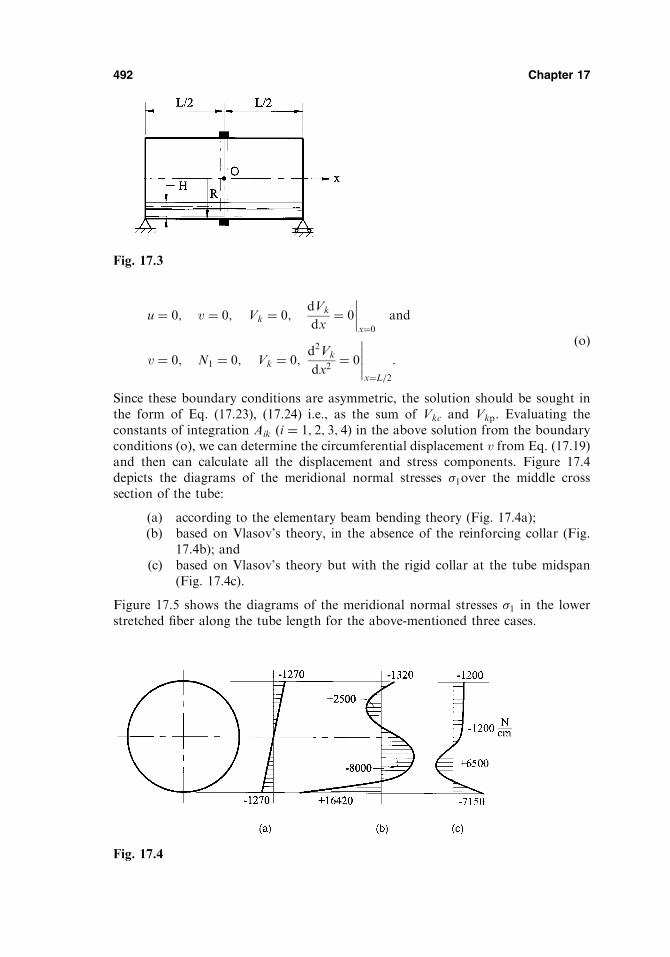
u ¼ 0; v ¼ 0; Vk ¼ 0;dVk

dx¼ 0

x¼0

and

v ¼ 0; N1 ¼ 0; Vk ¼ 0;d2Vk

dx2¼ 0

x¼L=2

:

ðoÞ

Since these boundary conditions are asymmetric, the solution should be sought inthe form of Eq. (17.23), (17.24) i.e., as the sum of Vkc and Vkp. Evaluating theconstants of integration Aik ði ¼ 1; 2; 3; 4Þ in the above solution from the boundaryconditions (o), we can determine the circumferential displacement v from Eq. (17.19)and then can calculate all the displacement and stress components. Figure 17.4depicts the diagrams of the meridional normal stresses �1over the middle crosssection of the tube:

(a) according to the elementary beam bending theory (Fig. 17.4a);(b) based on Vlasov’s theory, in the absence of the reinforcing collar (Fig.

17.4b); and(c) based on Vlasov’s theory but with the rigid collar at the tube midspan

(Fig. 17.4c).

Figure 17.5 shows the diagrams of the meridional normal stresses �1 in the lowerstretched fiber along the tube length for the above-mentioned three cases.

492 Chapter 17

Fig. 17.3

Fig. 17.4

The last two solutions (for Cases b and c) were obtained by retaining fourterms in the expansion (m).

Comparing the bending stress diagrams depicted in Figs 17.4 and 17.5, oneconcludes that:

(a) Stresses in the shell for the given loading differ significantly from thosecalculated by the elementary beam bending theory.

(b) The bending stresses are noticeably reduced if a rigid collar, preventing adistortion of the tube cross section, is present. The character of the stressdistribution is also changed.

This example was taken from Ref. [6].If a large number of rigid collars were placed over the shell length in such a way

that all its cross sections remained circular and undistorted, the deformations andstresses would not be different from those calculated by the beam bending theory.Based on the above, one can conclude that the most efficient way of decreasingstresses in shell structures is to attach rigid collars to the shells. If a shell is loadedby a concentrated force, normal to the shell middle surface, then it is sufficient to setup only one rigid collar at a place of the force application. In this case, the shell willdeform as a beam, i.e., without distortion of its cross section.

In conclusion, let us discuss some issues regarding accuracy and area ofapplication of the semi-membrane theory. It was indicated earlier (see Chapter 13)that the accuracy of solutions given by the membrane theory depends on the smooth-ness of a shell geometry, the smoothness of an applied loading, and on the formula-tion of boundary conditions. However, for a cylindrical shell, in addition to theserequirements, one more requirement is added – namely, a shell length (see Sec. 13.6).It was shown in that section that the accuracy of the membrane solution decreaseswith an increase in the shell length, even if the other requirements of the existence ofthe membrane state of stress are satisfied. From a physical point of view, this meansthat for a long cylindrical shell the boundary conditions have little effect on thestresses and deformations in its middle part and these boundary conditions cannotprevent the appearance of significant bending stresses in this part of the shell (if anexternal loading is capable of causing the bending stresses).

Thus, the semi-membrane theory holds an intermediate place between themembrane theory and the general theory of thin shells (see Chapter 12). It can beapplied to relatively long open and closed cylindrical shells with an arbitrary shapeof the cross section if the variation of the displacement and stress components in thedirection of the shell generator is smoother than their variation in the circumferential


Fig. 17.5

direction. It follows from the above that a simple criterion for an estimate of theaccuracy of solutions of the semi-membrane theory can be established. This criterionlies in the comparison of @2f =@x2 and @2f =@�2 (where f is any displacement, strain,internal force, or stress component), according to the inequality (17.1).

It should be noted, however, that for very long shells, subjected to smoothlyvarying loads along their generator, distortions of the shell cross section can beneglected. Such shells may be treated as thin-walled bars. On other hand, forsmall values of L=R, the membrane theory is more accurate than the semi-membranetheory because the former theory takes into account the in-plane cross-section defor-mations "2 and �12. However, for very small values of L=R ðL=R < 3

ffiffiffiffiffiffiffiffiffih=R

p) [7], both

the theories are inapplicable because, in this case, the deformations vary rapidly inthe shell longitudinal direction. Finally, the semi-membrane theory can be recom-mended for medium-length cylindrical shells (L=2R ¼ 2� 8)

17.3 THE DONNELL–MUSHTARI–VLASOV THEORY OF THIN SHELLS

This section will continue the discussion about simplified theories of thin shells. Weintroduce below the Donnell [3], Mushtari [4], and Vlasov [1] theory (abbreviated asthe DMV theory). Conceptually, the DMV theory represents a simplified variant ofthe general linear theory of thin shells. Usually, this theory is based on the followingphysical assumptions (along with the Kirchhoff–Love hypotheses):

(a) the effect of the transverse shear forces Q1 and Q2 in the in-plane equili-brium equations is negligible (the static assumption);

(b) the influence of the deflections, w, will predominate over the influences of thein-plane displacements u and v in the bending response of the shell (thegeometric assumption).

It should be noted that the static and geometric assumptions agree well with eachother as predicted by the static–geometric analogy established for thin shells byGol’denveizer [5]. Further, it was shown by Novozhilov [2] that the above physicalassumptions are well justified in the following two cases:

1. A shell is shallow ( see Sec. 11.8.4).2. The state of stress is of such a type that displacements, and hence, stresses,

are rapidly varying functions at least in the direction of one of the coordi-nates and . As a result, the derivatives of these functions are signifi-cantly greater than the functions themselves – the second derivatives aregreater than the first derivatives, etc.

The second case is more general than the first case because it is applied not only toopen but also to closed shells, i.e., to essentially non-shallow shells.

A variation of any function f ðsÞ can be characterized by the order of the value

1

f ðsÞ df ðsÞds

� 1

b; ð17:27Þ

where b is a typical linear dimension of the shell and the symbol � indicates theidentity of the values order. It is assumed that the state of stress and strain of a shellis rapidly varying, say in the direction, if for any functions f ð; Þ (displacements,stress resultants, and and couples) the following strong inequality holds [2,5]:

494 Chapter 17

It can be shown that the first two equations of the above system are automaticallysatisfied if we substitute for �1; �2; and �12 from the kinematic relations (17.29).The third equation of the system (17.35), after substituting for "1; "2; and �12 fromEqs (12.45) together with Eqs (17.31), and for �1; �2; and �12 from Eqs (17.29),and after some transformations with the use of the Codazzi–Gauss relations, takesthe form

r2r2�þ Ehr2kw ¼ 0: ð17:33bÞ

Thus, the system of the governing differential equations of the approximate DMVtheory of thin shells have the following form:

�r2k�þDr2r2w ¼ p3;

r2r2�þ Ehr2kw ¼ 0:

ð17:36Þ

The first equation of the above system is the equilibrium equation, whereas thesecond one represents the compatibility equation. For a flat plate, �1 ¼ 0 and�2 ¼ 0, and therefore, r2

kð. . .Þ ¼ 0. Hence, for flat plates, the first and second Eqs(17.36) are uncoupled. The second equation, r2r2� ¼ 0, determines the Airy stressfunction of the plane stress problem, and the second one, Dr2r2w ¼ p3, describesthe plate bending problem, as discussed in Part I of the book. The operator r2

k,depending upon the shell curvatures, characterizes in Eqs (17.36) the coupled effectbetween the bending and membrane stress resultants.

In conclusion, let us briefly discuss a practical application of the DMV theoryof thin shells. As mentioned previously, it can be applied to closed or open shells ofany geometry if the state of stress is rapidly varying, at least, in one direction. Itshould be noted that solutions of the membrane shell problem and problem of purebending are given by slowly varying functions. Therefore, the DMV theory can givea serious error in the stress analysis of such shell problems only if a shell area underconsideration is not small compared with the radius Rj jmin. The DMV theory can beapplied successfully to the analysis of thin shells whose state of stress is described byrapidly varying functions as, for instance, in the edge effect state of stress, discussedin detail in Sec. 17.5 for thin shells of any geometry. The DMV theory can also becorrectly applied to the stress analysis of the shallow shells introduced in the next

section. Lur’e [8] showed that the analysis of not too long LR� 0:75

ffiffiffiRh

q� �cylindrical

shells, based on the DMV theory, gives sufficiently accurate results even for slowlyvarying loads.

17.4 THEORY OF SHALLOW SHELLS

Shallow shells are frequently used for roof structures of industrial and public build-ings. They are also used in mechanical and aerospace engineering applications. Thetheory of shallow shells can be also used to analyze shells that become locallyshallow when the original shell is divided into finite segments or elements (see, forinstance, Chapter 19).

Shallow shells were introduced in Sec. 11.8.4. Let us define a shallow shell in amore rigorous manner. Take the Cartesian coordinates x and y of the projections ofpoints of the shell’s middle surface on the coordinate plane Oxy as curvilinear


coordinates and of that surface, i.e., define the middle surface of the shell by thefollowing equation:

z ¼ zðx; yÞ: ð17:37ÞThis can be done because of the single-valued correspondence of points of the middlesurface and their rectangular projections on the plane Oxy.

A shell may be called shallow if at any point of its middle surface the inequalities(11.58) hold.

If we confine our analysis to the accuracy of the theory of thin shells (seeinequality (10.1)), i.e., consider a shell as shallow for

@z

@x

� �2

< 0:05;@z

@y

� �2

< 0:05; ð17:38Þ

then the angle of 0.224 rad or � 13 may be taken as the limiting angle between thetangent plane to the shell’s middle surface and the coordinate plane Oxy. Notice thatVlasov [1] defined a shallow shell as a shell whose rise does not exceed 1/5 of thesmallest dimension of the shell in its plane (projection on the coordinate plane Oxy).However, it can be shown [2] that this practical limitation of the applicability of theshallow shell theory corresponds to the error noticeably exceeding the above-men-tioned error of 5%.

Consider an element of the middle surface ABCD (Fig. 11.15a). Let its projec-tion on the coordinate plane Oxy be the rectangle with sides dx and dy, as shown inFig. 11.15a. The sides of the element ABCD are the following:

ds1 ¼ffiffiffiffiffiffiffiffiffiffiffiffiffiffiffiffiffiffiffiffiffiffi1þ @z

@x

� �2s

dx; ds2 ¼ffiffiffiffiffiffiffiffiffiffiffiffiffiffiffiffiffiffiffiffiffiffi1þ @z

@y

� �2s

dy:

However, by virtue of the assumption (17.38), one can use the following approxima-tions:

ds1 � dx; ds2 � dy; ð17:39Þi.e., one can identify the increments of arcs of the coordinate lines on the shell’smiddle surface with the increments of the corresponding rectangular coordinates.The cosine of angle between the lines x and y is equal to

cosðds1^; ds2Þ ¼@z@x@z@yffiffiffiffiffiffiffiffiffiffiffiffiffiffiffiffiffiffiffiffiffi

1þ @z@x

� �2r ffiffiffiffiffiffiffiffiffiffiffiffiffiffiffiffiffiffiffiffi1þ @z

@y

� �2r :

It follows from the above that for shallow shells, again because of the inequalities(17.38), one can assume that

cosðds1^; ds2Þ � 0; ð17:40Þi.e., it is possible to consider the curvilinear system x; y as approximately orthogonal.The curvatures of the coordinate lines x and y, �1 and �2, and ‘‘twist,’’ �12, of theundeformed middle surface at any point of the middle surface of the shallow shellcan be identified with the second derivatives of Eq. (17.37), i.e.,

498 Chapter 17

�1 ¼1

R1

� @2z

@x2; �2 ¼

1

R2

� @2z

@y2; �12 �

@2z

@x@y: ð17:41Þ

Taking Eqs (17.39) and (17.40) as exact equalities, we obtain that the followingLame parameters for a shallow shell of any geometry:

A ¼ 1; B ¼ 1; ð17:42Þi.e., the intrinsic geometry of a shallow shell is identical to the geometry of a plane of itsprojection. This actually represents the first basic assumption of the theory of shallowshells. It follows from the above that the shallow shell has the Gaussian curvature� ¼ 1

R1R2� 0 because the latter is an exact zero only for flat plates. In particular cases

the Gaussian curvature of shallow shells is also exactly equal to zero (for instance, ifa shallow shell is a cylindrical or conical shell).

As mentioned in Sec. 17.3, the DMV theory can be applied to the analysis ofshallow shells. Hence, the next, second basic assumption of the theory of shallow shellsis the basic assumption of the more general DMV theory of neglecting the tangential(membrane) displacements u and v in the kinematic expressions for the changes incurvature and twist, Eqs (12.24) and the transverse shear forces Q1 and Q2 in the twofirst equations of equilibrium (12.41) (see Sec. 17.3).

The DMV theory, as the general theory of thin shells, was constructed in termsof the lines of curvature as curvilinear coordinate lines. Therefore, from now on,assume that the coordinate lines x and y coincide with the lines of curvature of theshell’s middle surface. The error of this assumption is not beyond the limits of theaccuracy of the shallow shell theory.

The shallowness of shells makes it possible to make further simplifications tothe DMV theory. Making ¼ x; ¼ y; and A ¼ B ¼ 1, we obtain the followingrelations for the strain components (Eqs (12.23)) and changes in curvature (Eqs(12.24)):

"1 ¼@u

@x� w

R1

; "2 ¼@v

@y� w

R2

; �12 ¼@v

@xþ @u@y;

�1 ¼ � @2w

@x2; �2 ¼ � @

2w

@y2; �12 ¼ � @2w

@x@y:

ð17:43Þ

The Laplace operator (17.34a) is easily simplified to the form

r2ð. . .Þ � @2ð. . .Þ@x2

þ @2ð. . .Þ@y2

: ð17:44aÞ

The Codazzi conditions (11.27a) for shallow shells, and taking into account Eqs(17.42), are

@

@

1

R1

� �¼ 0 and

@

@

1

R2

� �¼ 0:

Also, the Vlasov operator r2k, introduced in Sec. 17.3 (see Eq.(17.34b)), taking into

account the above relations, can be simplified to the following form:

r2kð. . .Þ �

1

R2

@2ð. . .Þ@x2

þ 1

R1

@2ð. . .Þ@y2

¼ �1@2ð. . .Þ@x2

þ �2@2ð. . .Þ@y2

: ð17:44bÞ


Although the operators r2 and r2k were notably simplified, the system of governing

equations for the theory of shallow shells will be of the same form as the system ofequations (17.36) derived in Sec. 17.3 for the general DMV approximate theory ofthin shells.

Solving the system of differential equations (17.36), gives � and w. Havingdetermined the above functions, we can then determine the internal forces andmoments using Eqs (17.31), (17.29) and (12.46). Let us present below all theseequations for shallow shells, as follows:

N1 ¼@2�

@y2; N2 ¼

@2�

@x2; S ¼ � @2�

@x@y; ð17:45aÞ

M1 ¼ �D@2w

@x2þ � @

2w

@y2

!; M2 ¼ �D

@2w

@y2þ � @

2w

@x2

!;

H ¼ �ð1� �Þ @2w

@x@y; ð17:45bÞ

Q1 ¼ �D@

@xðr2wÞ; Q2 ¼ �D

@

@yðr2wÞ:

The solution of Eqs (17.36) must satisfy the boundary conditions prescribedon the shell edges. We present below some typical boundary conditions for ashallow shell of an arbitrary geometry whose boundaries form a rectangularplane. For the sake of simplicity, assume that the shell edges coincide with thex- and y-coordinate lines and these lines are the lines of curvature. As mentionedpreviously, Eqs (17.36) have the eighth order, so the four boundary conditionsmust be prescribed on each edge of the shell (by two conditions on each of thefunctions � and w). Let us consider the boundary conditions for the shell edge x ¼const: Note that the boundary conditions, depending on the shell deflections, havethe same form as that for flat plates (see Eqs (2.48)). Therefore, we introducebelow some typical boundary conditions imposed on the function � (or on thein-plane displacements in the directions of the x and y axes, u and v). We have (forexample, for the shell edge x ¼ const.)

(a) Points of the shell edge can freely displace in the direction of the x axis.This means that

N1 ¼ 0 or@2�

@y2¼ 0: ð17:46aÞ

(b) Points of the shell edge can freely displace in the direction of the y axis.Then, we have

�12 ¼ 0 or@2�

@x@y¼ 0: ð17:46bÞ

(c) No displacements of the shell edge are allowed in the x direction, i.e.,

u ¼ 0: ð17:47aÞ

500 Chapter 17

(d) No displacements of the shell edge are allowed in the y direction, i.e.,

v ¼ 0: ð17:47bÞ

In solving real design problems, various combinations of these boundary conditionscan be met. For example, for a clamped shell edge that is parallel to the y axis, theboundary conditions are given by

u ¼ v ¼ w ¼ @w

@x¼ 0: ð17:48Þ

If a shell edge rests on a diaphragm that is absolutely rigid in its own plane andflexible out of the plane, the boundary conditions have the form

@2�

@y2¼ 0; v ¼ w ¼ @2w

@x2¼ 0: ð17:49aÞ

If a shell edge can displace freely along this diaphragm, then we have

@2�

@y2¼ @2�

@x@y¼ 0; w ¼ @2w

@x2¼ 0: ð17:49bÞ

Similarly, the boundary conditions can be presented for the shell edge y ¼ const:For the analysis of shallow shells it is necessary to solve the system of equations

(17.36), satisfying the above boundary conditions for the functions w and �. For asolution of these equations, some analytical and numerical methods, introduced inChapter 6, may be applied. One of the most adapted analytical methods for solvingthis system of linear differential equations for a shallow shell with constant curva-tures whose edges form a rectangular plane is the Fourier method of double series,which is similar to the Navier method discussed in Sec. 3.3 for bending of rectangularplates. Variational methods are frequently used for analyses of shallow shells. Inorder to apply the variational methods introduced in Chapter 6, let us set up theexpression for the strain energy of shallow shells. Substituting for N1;N2; and Sfrom Eqs (17.45a) and for M1;M2; and H from Eqs (17.45b) into Eq. (12.52) andsetting A ¼ B ¼ 1, we obtain the following expression for the strain energy of shal-low shells:

U ¼ 1

2Eh

ð ðA

@2�

@x2þ @

2�

@y2

!( 2

� 2ð1þ �Þ @2�

@x2@2�

@y2� @2�

@x@y

!224

359=;dA

þð ð

A

D

2

@2w

@x2þ @

2w

@y2

!2

�2ð1� �Þ @2w

@x2@2w

@y2� @2w

@x@y

!224

35

8<:

9=;dA;

ð17:50Þwhere A is the area of the middle surface of the shallow shell.

Writing the corresponding expressions for work done by external loads, We,and the total potential energy, �, we can apply the Ritz method (see Sec. 6.6) forsolving various problems of shallow shell analysis.


17.5 THE THEORY OF EDGE EFFECT

In this section we introduce one more approximate theory of thin shells. As men-tioned in Sec. 17.3, a thin shell can be found in the basic state of stress that ischaracterized by slowly varying deformations and stresses. The membrane (seeChapters 13 and 14) and pure bending stress states fall into the category of thebasic state of stress. The pure bending state rarely occurs. It is possible for nonrigidshells only whose constraints allow such a type of bending. In some cases, the state ofstress in thin shells can be separated into the following two components: the basic(mainly, membrane) for the entire shell and the mixed, mostly, a moment state, callededge effect, localizing near shell boundaries or near other sites at which the membranetheory does not apply. The latter state of stress can be superimposed on the basic statethat essentially simplifies the obtaining of the general state of stress in a shell. It wasindicated in Chapters 13–16 that the membrane solution alone for some shell geome-tries, loadings, and supports cannot satisfy the prescribed boundary conditions at theshell edges, the known conditions of continuity, equilibrium and/or kinematic con-straints at the edge effect zones. Gol’denveizer termed the sources of edge effects‘‘lines of distortion.’’ To facilitate their identification, Gol’denveizer listed these as [5]:

(a) the physical edges of a shell;(b) lines along which discontinuities of the components of external loads or

of certain their derivatives occur;(c) lines along which the middle surface of a shell has a break or the curva-

ture of the middle surface changes abruptly; and(d) lines along which the rigidity of a shell or its thickness undergoes sudden

changes.

The edge effect can be defined as such a state of stress and strain at which stresses anddisplacements vary slightly along the lines of distortion, but decay rapidly in the normaldirection to those lines.

The edge effect concept was demonstrated in Chapters 15 and 16 for axisym-metrically loaded circular cylindrical shells and shells of revolution, respectively.This section is concerned with constructing the general theory of the edge effectfor shells of any geometry subjected to asymmetric loading.

In deriving the governing differential equations of the theory of edge effect, wemake the following assumptions:

1. The lines of distortion coincide with one of the lines of curvature (fordefiniteness sake, with the -coordinate line).

Let us introduce the so-called asymptotic line as a line along which thenormal curvature of the surface, 1=Ri, is zero. For example, a generatorof a cylindrical surface can be considered as an asymptotic line. In thetheory of edge effect, it is assumed that the lines of distortion at any pointof the middle surface do not touch the asymptotic line. In this case, theedge effect always takes place and it is called simple edge effect. If thedistortion line touches an asymptotic line, then such an edge effect isreferred to as a complex one. In this section we analyze only the simpleedge effect.

2. The normal component of displacement, w, in zones of the edge effect issignificantly greater than the in-plane components, u and v.


3. Functions f that characterize the state of stress and strain (displacements,internal forces, and moments) vary significantly more rapidly in the direc-tion of the -coordinate line than in the direction of the -coordinate line,i.e.,

@f

A@

� @f

B@

: ð17:51Þ

(4) The Lame parameters, A and B, as well as the radii of curvature, have asmall variation in the direction of the -coordinate line, i.e.,

@A

@� A;

@B

@� B;

@R1

@� R1;

@R2

@� R2:

ð17:52Þ

A rapid decay of the edge effect state of stress, as we move away along the normal tothe line of distortion is a very important characteristic of a shell. It is caused by theshell thinness and by the curvilinearity of its surface. Let us explain this phenomenonin more detail in the following simple example.

Figure 17.8 shows a flat cantilever plate and an open circular cylindrical shellloaded by uniformly distributed bending moments, m ¼ const, applied to the freeedges of the plate and shell.

It is evident, that the cantilever plate will resist the external moment load bymeans of bending only (producing the bending and twisting moments, and shearforces); no membrane forces occur in its middle surface (Fig. 17.8a). The cantilevershell will support the applied distributed moments m not only by means of the bend-ing but also by straining the middle surface. The latter is accompanied by an appear-ance of the circumferential membrane forces N2 in the longitudinal sections of theshell ’ ¼ const, i.e., in the sections perpendicular to the edge x ¼ a (Fig. 17.8b). Thelarger the shell curvature 1=R, the stiffer is the shell in its middle surface and thegreater is the role of the membrane forces N2 in resisting the applied bending load.The availability of the circumferential forces N2 will cause the internal bendingmoment to decrease rapidly as we move away from the loaded edge in the normaldirection to the edge. This phenomenon is quite understandable if we recall the

508 Chapter 17

Fig. 17.8

displacements and stresses that vary slowly and they are taken into account by themembrane and pure moment solutions). Integrating twice the second equation of thesystem (17.54) and discarding the arbitrary functions, one finds the following:

@

A@

@�

A@¼ �Eh

R2

w: ð17:55Þ

Substituting the above into the first Eq. (17.54) and putting Ad ¼ ds1, we bring thisequation to the form

@4w

@s41þ 12ð1� �2Þ

R22h

2w ¼ 0: ð17:56Þ

This is the governing homogeneous differential equation of the simple edge effect. Itdiffers from the corresponding equation of the axisymmetric edge effect in a circularcylindrical shell (see Eq. (15.43)) by the fact that the partial derivatives of w enter inthis equation, because w is a function of two variables (this function varies slowlyalong the curvilinear coordinate too).

A solution of Eq. (17.56), which decays, as we move away from the edge ¼ 0,is of the following form:

w ¼ e��s1 ½f1ðs2Þ cos �s1 þ f2ðs2Þ cos �s1�; ð17:57Þwhere f1 and f2 are some slowly varying functions, Bd ¼ ds2, and

� ¼ffiffiffiffiffiffiffiffiffiffiffiffiffiffiffiffiffiffi3ð1� �2Þ4

q1ffiffiffiffiffiffiffiffiR2h

p : ð17:58Þ

The internal forces and moments, which occur in the edge effect state, can bedetermined next. Using Eqs (17.29) and neglecting, due to the assumptions of theedge effect theory, the variation of the shell geometry in the zone of the simple edgeeffect, and also assuming that

@w

@s2� @w

@s1;

one finds that

�1 � � @2w

@s21; �2 � 0; �12 � 0:

Then, inserting the above into Eqs (12.46), we obtain

M1 ¼ �D@2w

@s21; M2 ¼ �M1; H ¼ 0: ð17:59Þ

The stress function � can be determined by integrating twice the first Eq. (17.54). Wehave

� ¼ R2D@2w

@s21: ð17:60Þ

The membrane forces N1;N2; and S are related to the function � by Eqs (17.31),which due to the adopted assumptions of the edge effect theory, result in the expres-sions

N1 � 0; N2 �@2�

@s21¼ R2D

@4w

@s41¼ �Eh

R2

w; S � 0: ð17:61Þ

510 Chapter 17

The transverse shear forces may be found from the corresponding equilibrium equa-tions of the DMV theory, i.e.,

Q1 ¼ �D@

A@ðr2wÞ; Q2 ¼ �D

@

B@ðr2wÞ:

Using the relations (17.53), the above relations appear, as follows:

Q1 ¼ �D@3w

@s31; Q2 � 0: ð17:62Þ

The above relations and equations of the general edge effect theory were introducedfor the case when the distortion line coincides with the -coordinate line. Similarly,the corresponding equations can be presented for the -coordinate line as a distor-tion line and, generally, for the case when the shell edge does not coincide with theline of curvature [5].

In conclusion, one notes the following:

1. The edge effect theory introduced above cannot be applied to the casewhen the shell boundary or another distortion line coincides with theasymptotic line.

2. If a considered state of stress and strain varies rapidly not only in thedirection of the normal to the shell boundary but also along the boundaryitself, the stress analysis of such a shell can be carried out by the DMVtheory introduced in Sec. 17.3.

3. The governing differential equation of the edge effect, Eq. (17.56), is onlyapproximate. The exact solution of the shell problems by the edge effecttheory requires an integration of the system of the partial differentialequations of the general theory of thin shells and therefore has no advan-tages from separation of a given state of stress into the membrane stateand edge effect. Thus, the latter is taken into account only approximately.

4. The solution (17.57) makes it possible to satisfy the two boundary con-ditions on the corresponding shell edge. It is evident that these boundaryconditions must be formulated for the sum of the membrane solution andthe solution given by Eq. (17.56).

PROBLEMS

17.1 Verify Eqs (17.12) and (17.16).

17.2 Specify the area of application of the semi-membrane theory to the analysis of open

and closed cylindrical shells.

17.3 A simply supported, at x ¼ 0 and x ¼ L, cylindrical tube is filled by water up to the

level H (Fig. 17.2). The tube is reinforced by two equally spaced, rigid along the tube

length, collars in such a way that they prevent a distortion of the tube cross sections.

Applying the semi-membrane theory, determine the axial normal stress, �1, distributionover the shell cross section where the collar is attached to the tube. Let L ¼ 30m; R ¼5:5m; h ¼ 5:0 cm; H ¼ 1:2m; E ¼ 210GPa, and � ¼ 0:3.

17.4 A simply supported, at x ¼ 0 and x ¼ L, closed circular cylindrical shell is subjected to

a uniform vertical line load q, as shown in Fig. P.17.1. Determine the axial normal

stress, �1, distribution in the lower stretched fiber along the shell length. Compare this


r2ð. . .Þ � 1

r

@

@rr@ð. . .Þ@r

� �þ 1

r

@2ð. . .Þ@2

" #;

r2kð. . .Þ �

1

r

@

@rrk2

@ð. . .Þ@r

� �þ @

@

k1r

@ð. . .Þ@

� �� :

ðP:17:4Þ

17.12 Show that the membrane forces N1;N2; and S in the shallow shell theory are expressed

in terms of the displacements, as follows:

N1 ¼ B@u

@xþ � @v

@y� ð�1 þ ��2Þw

� �; N2 ¼ B

@v

@yþ � @u

@x� ð�1 þ ��2Þw

� �;

S ¼ Bð1� �Þ2

@v

@xþ @u@y

� � ðP:17:5Þ

where

B ¼ Eh

1� �2 :

17.13 Using the equations of equilibrium (12.44), Eqs (17.45b), (P.17.5), and the relations

(17.42), show that the governing equations of the shallow shell of double curvature in

Cartesian coordinates are of the following form:

@2u

@x2þ 1� �

2

@2u

@y2þ 1þ �

2

@2v

@x@y� ð�1 þ ��2Þ

@w

@x¼ � p1

B;

1� �2

@2u

@x@yþ @2

@y2þ 1� �

2

@2

@x2

!v� ð�2 þ ��1Þw ¼ � p2

B;

@u

@xð�1 þ ��2Þ þ

@v

@yð�2 þ ��1Þ � ð�21 þ �22 þ 2��1�2Þw� h2

12r2r2w ¼ � p3

B:

ðP:17:6Þ

17.14 The governing equations (17.36) for the shallow shell theory were derived assuming

that p1 ¼ p2 ¼ 0; and p3 6¼ 0. Show that if all the load components are nonzero, the

relations (17.45a) should be replaced with

N1 ¼@2�

@y2�ðp1dx; N2 ¼

@2�

@x2�ðp2dy; S ¼ � @2�

@x@y; ðP:17:7Þ

and Eqs. (17.36) for this case appear as follows:

�r2k�þDr2r2w ¼ p3 � �1

ðp1dx� �2

Zp2dy;

r2r2�þ Ehr2kw ¼

ð@2p1@y2

dxþð@2p2@x2

dy� � @p1@x

þ @p2@y

� �:

ðP:17:8Þ

17.15 Consider a square in a plan shallow shell of double curvature. Let the equation of its

middle surface be given by (the origin of the Cartesian coordinate system is taken at the

center of the projection of the shell on the horizontal plane)

z ¼ f 1� x2 þ y2

2a2

!;

where f ¼ f1 þ f2 is the total rise. The shell edges, x ¼ �a and y ¼ �a, have the same

supports as described in Example 17.1. The shell is subjected to a uniformly distributed

load p. Determine the deflection w, the membrane forces N1;N2; and S, the bending

moments M1 and M2; and the twisting moment H. Take four terms (m ¼ 1; n ¼ 1; m


¼ 1; n ¼ 3; m ¼ 3; n ¼ 1; m ¼ 3; n ¼ 3Þ in the expansions (e) and (f) in Example 17.1.

Let a ¼ 2:0m; h ¼ 20mm; f1 ¼ f2 ¼ 250mm; p ¼ 2 kPa; G ¼ 30GPa; and � ¼ 0.

17.16 A shallow shell of double curvature, shown in Fig. 17.6, is supported by diaphragms at

its edges (the boundary conditions are given by Eqs (c) and (d) in Example 17.1). The

shell is subjected to a uniformly distributed load of intensity p: Determine the deflec-

tions, in-plane forces, and bending moments in the shell. Take four terms in the

expansions (e) and (f) (see problem 17.15). Take a ¼ 10m; b ¼ 12m; �1 ¼ 0:04=l;m;�2 ¼ 0:02781=m, h ¼ 30mm; E ¼ 22GPa; and � ¼ 0:

17.17 Show that if deflection w is a rapidly varying function, at least in one of the coordinate

directions, then the following estimate takes place:

r2w w

R1R2

� C2

where C � 1.

17.18 Based on the results of Problem 17.7, derive Eqs (17.62).

17.19 Specify the area of application of the edge effect theory for open and closed cylindrical

shells loaded asymmetrically.

REFERENCES

1. Vlasov, V.Z., General Theory of Shells and its Applications in Engineering, NASA

Technical Translation TTF-99, Washington DC, 1964.

2. Novozhilov, V.V., Thin Shell Theory (translated from 2nd Russian edn. by P.G. Lowe),

Noordhoff, Groningen, The Netherlands, 1964.

3. Donnell, L.H., Stability of Thin Walled Tubes under Torsion, NACA, Report No. 479,

Washington, DC, 1933.

4. Mushtari, Kh.M., Certain generalizations of the theory of thin shells, Izv Fiz Mat ob-va pri

Kaz Un-te, vol. 11, No. 8 (1938) (in Russian).

5. Gol’denveizer, A.L, Theory of Elastic Shells (translated from Russian by G. Herrmann),

Pergamon Press, New York, 1961.

6. Boyarshinov, S.V., The Fundamentals of Structural Mechanics of Machines,

Mashinostroenie, Moscow, 1973 (in Russian).

7. Biderman, V. L., Mechanics of Thin-Walled Structures, Izdatel’stvo ‘‘Mashinostroenie’’,

Moscow, 1977 (in Russian).

8. Lur’e, A.L., General theory of elastic shells, Prikl Mat Mekh, vol. 4, No. 1, pp. 7–34

(1940) (in Russian).

514 Chapter 17

18

Advanced Topics

18.1 THERMAL STRESSES IN THIN SHELLS

18.1.1 General

This section is concerned with the influence of high temperature on the state of stressand strain in thin shells. This issue has been studied in Sec. 7.1, as applied to thinplates. It should be noted that the thermal stresses and deformations in thin shells area major factor in the design of structures such as boilers, heat exchangers, pressurevessels, nuclear piping, and supersonic aircraft skin. The basic concepts of the ther-moelastic stress analysis of thin shells are quite similar to those introduced in Sec. 7.1for thin plates. Similarly, the thermoelastic problems require modifying the consti-tutive equations of the general shell theory.

Let a shell be subjected to a nonuniform temperature field Tð; ; zÞ measuredfrom some specified reference value. The temperature distribution T can be obtainedfrom a solution of the equation of heat conduction [1], represented in terms of theshell coordinates. Taking into account the relations (7.1), we can modify the con-stitutive equations (12.28) by taking into account the temperature effects, as follows:

"z1 ¼1

E�z1 � ��z2ð Þ þ T; "z2 ¼

1

E�z2 � ��z1ð Þ þ T; �z12 ¼

1

G�z12; ð18:1Þ

where is the coefficient of thermal expansion (see Sec. 7.1). It is assumed that E; �,and d are constant for a given temperature field. Solving Eqs (18.1) for the stresscomponents yields

�z1 ¼E

1� �2 "z1 þ �"z2 � ð1þ �ÞT½ �; �z2 ¼

E

1� �2 "z2 þ �"z1 � ð1þ �ÞT½ �;

�z12 ¼ G�z12:

ð18:2Þ

515

The technique of integrating Eq. (18.11) is not different from that discussed in Sec.15.3.

As mentioned previously, the thermal terms on the right-hand side of Eq.(18.11) can be interpreted as some fictitious surface load, qT . So, we can rewriteEq. (18.11), as follows:

d4w

dx4þ 44w ¼ 1

Dp3 � qT þ �N1

R

� �; ð18:13Þ

where

qT ¼ Dð1þ �Þh

d2ð�TÞdx2

þ Eh

RT0: ð18:14Þ

Using the principle of superposition, the given thermoelastic problem for a circularcylindrical shell can be broken down into two independent problems. The firstproblem involves only thermal effects produced by qT . In this case, only the parti-cular solution is of interest (all constants of integration are assumed to be zero). Thesecond problem deals with external forces, p3 and N1. Its solution was presented inSec. 15.3. The constants of integration are evaluated in such a way that the sum ofthe solutions of these two problems satisfies the prescribed boundary conditions.

Example 18.1

An infinitely long circular cylindrical shell is heated according to Eq. (18.6). Thetemperature is a constant along the shell length. Determine the thermal stresses.

Solution

A given thermal field can be represented as a superposition of a uniform heatingT0 ¼ ðT1 þ T2Þ=2, which produces no stresses, and of the thermal change�T ¼ T1 �T2 (Fig. 18.1).

Let us consider the state of stress corresponding to the thermal jump men-tioned above. Since the temperature does not vary along the shell length, then allvalues are constant over the length, and, hence, a general solution of the thermalhomogeneous equation is nonexistent. The particular solution (Eq. (18.12)) forp3 ¼ 0, N1 ¼ 0, and T0 ¼ 0 is also zero. Thus, the deflections of points of the middlesurface w and the circumferential force N2, according to Eq. (18.8b), are also equal

518 Chapter 18

Fig. 18.1

the bending moments at shell edges, as shown in Fig. 18.2b. These moments can becalculated from Eqs. (18.15):

– for the first part of the shell ðh ¼ h1Þ,

Mð1Þ1ð�TÞ ¼ ��Tð1þ �ÞD1

h1¼ � �TEh21

12ð1� �Þ ¼ �8000 N �m=m;

– for the second part of the shell ðh ¼ h2Þ,

Mð2Þ1ð�TÞ ¼ ��Tð1þ �ÞD2

h2¼ � �TEh22

12ð1� �Þ ¼ �2000 N �m=m:

At a state shown in Fig. 18.2c, the shell is loaded by the interface moments, M0 andshear forces, Q0 at the junction of the two shell parts only, where M0 and Q0 are theinterface bending moment and shear force that actually act at the junction of thestepped shell and M

ð1Þ1ð�TÞ and M

ð2Þ1ð�TÞ have been added to compensate the moments

applied to the shell in the state shown in Fig. 18.2b. To determine the interfacemoment M0 and shear force Q0, it is sufficient to consider only the state shown inFig. 18.2c and set up the conditions of compatibility for deformations at the junctionof the two shell parts. The latter are of the following form:

wð1Þ ¼ wð2Þ; #ð1Þ1 ¼ �#ð2Þ1 ; ðaÞi.e., the deflections and slopes of the normals for the two shell parts at the junctionshould be the same. The negative sign in Eq. (a) is taken because the direction of thex axis for the first and second parts of the shell is opposite. The deflections, wð1Þ andwð2Þ, and slopes, #ð1Þ1 and #ð2Þ1 , may be determined from Eqs (15.57). For the first (left)shell part, setting x ¼ 0 and wp ¼ 0, we obtain

wð1Þ ¼ �M0 þMð1Þ1ð�TÞ

2D121

þ Q0

2D131

; #ð1Þ1 ¼ M0 þMð1Þ1ð�TÞ

D11� Q0

2D121

: ðbÞ

Similarly, for the second shell part, again setting x ¼ 0 and wp ¼ 0, we have thefollowing:

wð2Þ ¼ �M0 þMð2Þ1ð�TÞ

2D222

� Q0

2D232

; #ð2Þ1 ¼ M0 þMð2Þ1ð�TÞ

D22þ Q0

2D222

: ðcÞ

Computing the geometric properties of the stepped shell, we have

D1 ¼Eh31

12ð1� �2Þ ¼ 146:8 kN �m; D2 ¼Eh32

12ð1� �2Þ ¼ 18:33 kN �m

or D2 ¼D1

8;

1 ¼ 4

ffiffiffiffiffiffiffiffiffiffiffiffiffiffiffiffiffi3ð1� �2R2h21

s¼ 12:85

1

m; 2 ¼ 4

ffiffiffiffiffiffiffiffiffiffiffiffiffiffiffiffiffiffi3ð1� �2ÞR2h22

s¼ 18:13

1

m¼ 1

ffiffiffi2

p;

Mð1Þ1ð�TÞ ¼ 8000N �m=m; M

ð2Þ1ð�TÞ ¼ 2000N �m=m ¼ 1

4M

ð1Þ1ð�TÞ:

520 Chapter 18

considerably less than the other linear dimensions of the shell (from now on, the term‘‘geometrically’’ will be dropped because only this type of nonlinearity is discussedherein). The large-displacement theory of thin plates and shells originates from vonKarman’s work [2]. E. Reissner developed the geometrically nonlinear theory of thinshells [3]. Considerable contributions in the nonlinear shell theory were made bySaunders [4], Mushtari [5], etc. We will present here Vlasov’s approach for derivingthe governing differential equations of the nonlinear shallow shell theory [6].

A geometric nonlinearity manifests to the theory in twoways. At first, because ofmoderately large displacements, the strain components are related to these displace-ments by means of nonlinear equations. Secondly, a shell element undergoes so muchchanges in its shape after deformation, i.e., it moves and rotates in space through suchfinite distances and angles, that it is impossible to set up its equilibrium equations basedon an undeformed shell configuration as has been done in the linear shell theory.

18.2.2 Nonlinear theory of shallow shells

As in the classical shell theory, assume that the coordinate lines coincide with thelines of principal curvatures. We start the nonlinear shallow shell analysis with thestrain–displacement relations. In the classical, linear shell theory, it was assumed thatstrains were small and that the rotations were of the same order of magnitude as thestrains. As mentioned earlier, the above rotations should be taken into account indeveloping the kinematic relations of the nonlinear theory of shallow shells.However, it will be assumed that the nonlinear strains of the middle surface remainstill small compared with unity and they are of the order of the rotations squared.

It follows from the above that the nonlinear theory deals with the more compli-cated strain–displacement equations. However, for shallow shells, these equations canbe simplified. Indeed, since the geometry of a shallow shell is close to a flat plate, thestiffness of the shell in the tangent plane is significantly greater than the flexural stiff-ness (see Sec. 7.4.1). Therefore, say, the angle of rotation !1 of the element ds1 in thetangential plane (about the unit vector e3) is much smaller than the angle of rotation #1of the same element in the normal plane (about the unit vector e2). However, althoughthe angles #1 and #2 are larger inmodulus than the angles!1 and !2, the former anglesthemselves remain still small because of the following limitation for the deflectionsadopted in the nonlinear theory of shallow shells: wj j � 5h. Therefore, the squares ofthe angles #1 and #2 can be neglected in comparison with unity.

Thus, the basic assumption of the linear shell theory about the smallness of thesquares of all the angles of rotation compared with unity and about the equivalenceof orders of their values is now reduced and it is postulated that

!21 � #21 � 1;!2

2 � #22 � 1: ð18:18ÞAs a result of the above assumption, the strain–displacement relations of the lineartheory of shallow shells, Eqs (17.43), are complemented by the same nonlinear termsas in the theory of flexible plates (see Eqs (7.82)):

"1 ¼@u

@x� w

R1

þ 1

2

@w

@x

� �2

; "2 ¼@v

@y� w

R2

þ 1

2

@w

@y

� �2

;

�12 ¼@u

@yþ @v

@xþ @w@x

@w

@y:

ð18:19Þ

Advanced Topics 523

Notice that the shear strain expression for shallow shells is absolutely identical tothat obtained in the large-deflection theory of thin plates (see the third Eq. (7.82)).Hence, the shell curvature does not affect the shear deformation of the middle sur-face, if the coordinate lines x and y are the lines of the principal curvatures in theframework of the theory of shallow shells.

The expressions for changes in curvature and for twist of the middle surfacealso coincide with those obtained in the small-deflection theory of shallow shells, i.e.,

�1 ¼ � @2w

@x2; �2 ¼ � @

2w

@y2; �12 ¼ � @2w

@x@y: ð18:20Þ

The tangential strain components, "z1; "z2; and �

z12, at points in an equidistant surface

of the shell from the z coordinate, are determined, as previously, by Eqs (12.22).The expressions for the stress resultants and stress couples, as well as the

constitutive equations of the nonlinear shallow shell theory remain identical tothose introduced in Sec. 12.3 for the linear shell theory. Introducing the relations(18.19) into the constitutive equations (12.45) and letting N12 ¼ N21 ¼ S, we obtainthe following relations between the membrane forces and displacements at points ofthe middle surface:

N1 ¼Eh

1� �2@u

@xþ � @v

@yþ 1

2

@w

@x

� �2

þ �2

@w

@y

� �2

� w

R1

� � w

R2

" #;

N2 ¼Eh

1� �2@v

@yþ � @u

@xþ 1

2

@w

@y

� �2

þ �2

@w

@x

� �2

� w

R2

� � w

R1

" #;

S ¼ Eh

2ð1þ �Þ@u

@yþ @v

@xþ @w@x

@w

@y

� �:

ð18:21Þ

Let us eliminate the tangential displacements u and v from Eqs (18.21), and expressthe forces N1;N2; and S in terms of the deflections w. For this purpose, first, trans-form the two first relations (18.21), as follows:

N1 � �N2 ¼ Eh@u

@xþ 1

2

@w

@x

� �2

� w

R1

" #; N2 � �N1 ¼ Eh

@v

@yþ 1

2

@w

@y

� �2

� w

R2

" #:

ð18:22ÞUsing the above relations, set up the following equation:

@2

@y2ðN1 � �N2Þ þ

@2

@x2ðN2 � �N1Þ � 2ð1þ �Þ @

2S

@x@y

¼ Eh@2

@y21

2

@w

@x

� �2" #

þ @2

@x21

2

@w

@y

� �2" #

� @2

@x@y

@w

@x

@w

@y

� �(

� 1

R1

@2w

@y2� 1

R2

@2w

@x2

�:

524 Chapter 18

According to the general rules of differentiating, the following equalities hold:

@2

@y21

2

@w

@x

� �2" #

¼ @2w

@x@y

!2

þ @w@x

@3w

@x@y2;@2

@x21

2

@w

@y

� �2" #

¼ @2w

@x@y

!2

þ @w@y

@3w

@x2@y;

@2

@x@y

@w

@x

@w

@y

� �¼ @3w

@x2@y

@w

@yþ @2w

@x@y

!2

þ @2w

@x2@2w

@y2þ @w@x

@3w

@x@y2:

Inserting these equalities in the above equation yields the following:

@2

@y2ðN1 � �N2Þ þ

@2

@x2ðN2 � �N1Þ � 2ð1þ �Þ @

2S

@x@y

¼ Eh@2w

@x@y

!2

� @2w

@x2@2w

@y2� 1

R1

@2w

@y2� 1

R2

@2w

@x2

24

35:

ð18:23Þ

Equation (18.23) represents the equation of compatibility of deformations of the non-linear shallow shell theory in terms of the membrane forces and deflections.

Let us introduce the stress function � according to the relations (17.45a).Substituting for � from the above relations into Eqs (18.23), results in

r2r2� ¼ Eh@2w

@x@y

!2

� @2w

@x2@2w

@y2� r2

kw

24

35; ð18:24Þ

where the operators r2 and r2k are given by Eqs (17.44).

Now we are coming to constructing the equations of equilibrium for ashallow shell element subjected to a transverse surface load p3. The positivedirections of the internal forces and moments acting on the element are shownin Fig. 12.5. The derivation of the equations of equilibrium in the nonlineartheory of shallow shells has some peculiarities. The force summations in the xand y directions, as well as the moment summations about the above axes, are setup as for the linear shell theory. This involves neglecting the changes in transitionof the shell element from its initial (undeformed) to the deflected state, and theinitial curvatures of the above element are also neglected. However, the forcesummation into the z direction is set up by taking into account both the initialcurvatures of the element and its consequent distortion acquired as a result ofshell straining under action of applied loads. It can be shown that the aboveequation of equilibrium will have the form of the third Eq. (12.41), derived forthe linear shell theory, but complemented by the same terms as for the corre-sponding equilibrium equation of the nonlinear theory of flat plates (see Eq.(3.91). The system of simplifications adopted in the nonlinear shallow shell theoryresults in the following equations of equilibrium:

@N1

@xþ @S@y

¼ 0;

@N2

@yþ @S@x

¼ 0; ð18:25Þ

Advanced Topics 525

@Q1

@xþ @Q2

@y¼ �p3 �

N1

R1

�N2

R2

�N1

@2w

@x2�N2

@2w

@y2� 2S

@2w

@x@y; ð18:26Þ

Q1 ¼@M1

@xþ @H@y

; ð18:27aÞ

Q2 ¼@M2

@yþ @H@x: ð18:27bÞ

Using the relations (18.27), it is possible to eliminate the shear forces Q1 andQ2 from Eq. (18.26). As a result, the equations of static equilibrium of theelement of a shallow shell in the nonlinear theory are reduced to the followingequations:

@N1

@xþ @S@y

¼ 0;

@N2

@yþ @S@x

¼ 0;

@2M1

@x2þ 2

@2H

@x@yþ @

2M2

@y2þN1

1

R1

þ @2w

@x2

!þN2

1

R2

þ @2w

@y2

!þ 2S

@2w

@x@yþ p3 ¼ 0:

ð18:28ÞSubstituting for the bending and twisting moments from Eqs (17.45b) into the thirdEq. (18.28) and introducing again the stress function � from Eq. (17.45a), we obtainthat the first two equations of (18.28) will be identically satisfied and the thirdequation becomes

Dr2r2w� r2k�þ @2�

@y2@2w

@x2þ @

2�

@x2@2w

@y2� 2

@2�

@x@y

@2w

@x@y

!" #¼ p3: ð18:29Þ

Eqsuations (18.24) and (18.29) are the governing differential equations of the non-linear theory of shallow shells. By introducing the operator

LðU;VÞ � @2U

@x2@2V

@y2� 2

@2U

@x@y

@2V

@x@yþ @

2U

@y2@2V

@x2; ð18:30Þ

we can rewrite the governing equations (18.24) and (18.29), as follows:

r2r2� ¼ �Eh1

2Lðw;wÞ þ r2

kw

� �;

Dr2r2w� r2k�þ Lð�;wÞ� � ¼ p3:

ð18:31Þ

Letting in Eqs (18.31) �1 ¼ 1=R1 ¼ 0 and �2 ¼ 1=R2 ¼ 0, we obtain Eqs (7.87) forthe large-deflection theory of plates. Boundary conditions on edges of the large-deflection shallow shell are formulated in a similar manner to those of the small-deflection shallow shell or of the large-deflection plate (see Secs 17.4 and 7.4, respec-tively).

526 Chapter 18

In conclusion, let us formulate some qualitative considerations about themechanical behavior of a geometrically nonlinear shell under applied loading. Forsimplicity, consider a flexible spherical shallow shell. Such a shell is governed by Eqs(18.31), if we let R1 ¼ R2 ¼ R. We obtain the following system of equations:

1

Ehr2r2�þ 1

2Lðw;wÞ þ 1

Rr2w

� �¼ 0;

Dr2r2w� 1

Rr2�þ Lð�;wÞ

� �¼ p3:

ðaÞ

Assume that the stress function � is assigned in the first approximation, as follows:

� ¼ Aðp3Þ � w; ðbÞwhere Aðp3Þ is a function of loading only. Substituting for � from Eq. (b) into Eq.(a), one obtains

A

Ehr2r2wþ 1

Rr2wþ 1

2Lðw;wÞ ¼ 0;

Dr2r2w� A

Rr2w� ALðw;wÞ ¼ p3:

Eliminating the nonlinear term Lðw;wÞ from the above equations, we obtain thefollowing equation:

D r2r2wþ 1

Rr2w ¼ p 3; ðcÞ

where

D ðp3Þ ¼2A

EhþD

A; p 3 ¼

p3A: ðdÞ

The quantity D ðp3Þ is made up of the extensional stiffness Eh and the flexuralstiffness D. Therefore, it can be called the composite stiffness of the shell.Obviously, the latter depends on the loading p3.

For a flexible plate, R ¼ 1, and Eq. (c) becomes

D r2r2w ¼ p 3: ðeÞEquations (c) and (e) are linear equations. Thus, a geometrically nonlinear shell orplate can be considered as a linear system whose flexural and extensional stiffnessesare replaced with some variable composite stiffness, D, given by the first Eq (d) anddepending on the applied loading. The above consideration can be used for anapproximate shell or plate analysis.

Example 18.3

Analyze the state of stress and strain in a cylindrical shallow shell of radius R havinga rectangular configuration in a plan (see Fig. 18.3a). Assume that the shell islengthened in the y direction (b � a) and is subjected to a uniform transverse surfaceload of intensity p. The straight edges of the shell are hinged and the displacementalong the x axis is eliminated.

Advanced Topics 527

Solution

Let us confine our study to the analysis of the middle part of the shell that issufficiently remote from the short curvilinear edges. A curved surface of this partof the shell can be considered as a cylindrical surface. Just as has been done for thecylindrical bending of flat plates (see Sec. 3.2.1), the bending of the given part of theshell will be identical to the bending of a unit curvilinear, simply supported at x ¼ 0and x ¼ a, shallow strip, isolated from the shell. For such a strip, w ¼ wðxÞ. Since thedeformations in the y direction of such a strip are restrained because of an interac-tion of neighboring strips, then it can be assumed that the relative deformation in they direction is zero, i.e., "2 ¼ 0. It can also be shown that the membrane force N1 ¼const over the shell width. The latter can be checked by considering the equilibriumof a shell element detached from the transverse shell strip, which is subjected to themembrane forces and given loading p, as shown in Fig. 18.3b. For a shallow shelland assumptions adopted in the nonlinear theory, the tangent to the curved axis ofthe shell strip can be neglected, i.e., it is possible to assume that N1 is a constant overthe shell width.

Thus, the equation of equilibrium (18.29) of the nonlinear shallow shell theoryacquires, in this particular case, the following form (taking into account thatN1 ¼ @2�=@y2Þ:

Dd4w

dx4�N1

d2w

dx2�N1

R¼ p: ð18:32Þ

The solution of this equation is sought in the form of the following series:

wðxÞ ¼X1m¼1

fm sinm�x

a: ð18:33Þ

It is evident that wðxÞ in the form of Eq. (18.33) satisfies the prescribed boundaryconditions for the deflections.

We solve the above problem in the first approximation, retaining the first termin the expansion (18.33) only. We apply the Galerkin method (see Sec. 6.5) for thesolution of Eq. (18.32). Let us introduce

528 Chapter 18

(a) (b)

Fig. 18.3

E � Dd4w

dx4�N1

d2w

dx2þ 1

R

!� p ¼ 0: ð18:34Þ

Write the Galerkin equation (6.38) in the formða0

E sin�x

adx ¼ 0: ð18:35Þ

Substituting for w from Eq. (18.33) into the above and retaining only one term in theexpansion, one finds the following after integration:

Df1�5

4a4þN1 f1

�3

a3� 1

R

!� p ¼ 0: ð18:36Þ

Determine the expression for the constant membrane force N1. From the first Eq.(18.19), one obtains

@u

@x¼ "1 þ

w

R� 1

2

@w

@x

� �2

: ð18:37Þ

Integrating the above over the width of the shell, yields the following:

uðaÞ � uð0Þ ¼ða0

"1 þw

R� 1

2

@w

@x

� �2" #

dx: ð18:38Þ

The given boundary conditions prescribed along the straight edges of the shell are ofthe form

w ¼ 0jx¼0;a;@2w

@x2¼ 0

x¼0;a

; u ¼ 0jx¼0;a:

Taking into account that "2 ¼ 0, we can obtain from the constitutive equations(12.45):

"1 ¼1� �2Eh

N1:

Substituting for "1 from the above relation into Eq. (18.38) and taking into accountthe boundary conditions, we can express the membrane force N1, as follows:

N1 ¼ � Eh

ð1� �2Þaða0

w

R� 1

2

@w

@x

� �2" #

dx:

Substituting for w from Eq. (18.33) into the above and integrating, we obtain (form ¼ 1Þ

N1 ¼Eh

1� �2f 21 �

2

4a2� 2f1�R

!: ð18:39Þ

Substituting the above expression into Eq. (18.36), we obtain the following cubicequation for the amplitude of deflections:

Advanced Topics 529

�5

16

f 31h3

� 3�2

4

f 21Rh3

þ �5

48þ 2a4

4R2h2

!f1h¼ ð1� �2Þ pa

4

Eh4: ð18:40Þ

The relationship between the dimensionless parameters p ¼ ð1� �2Þpa4=Eh4 andf1=h is illustrated in Fig. 18.4 (taken from Ref. [7]). The curves of this figure aregiven for various values of k ¼ a2=Rh. Figure 18.4 shows the four different plots;the straight line 1 indicates the relationship p of f1=h due to the linear theory ofshallow shells, whereas the three other curves describe the relationship in the large-deflection theory for various values of the parameter k .

It is seen that for a relatively small parameter k , the relationship p of f1=h issingle-valued (curve 2 refers to a flexible flat plate with k ¼ 0; and curve 3 stands fork ¼ 4:475). However, for larger values of this parameter (curve 4 stands fork ¼ 40) the above relationship is not uniquely defined, i.e., the three real roots ofEq. (18.40) correspond to one and the same value of p . This is a consequence ofsome peculiarities of straining the large-deflection shallow shell in the process ofincreasing the applied loading. As long as the parameter p increases from zero tothe value of 1025 (the ordinate of point A on the curve), the deflection amplitudegrows continuously up to the value � 2:2h, as is indicated by the branch OA of thecurve. However, as soon as the load parameter p becomes larger than a certainvalue (about 1025), the given cylindrical shallow shell undergoes the so-called snapthrough, i.e., the deflection changes its value by jumping from approximately 2:2h(the abscissa of point A on the curve) to approximately 11:1h (the abscissa of point Don the curve). Upon unloading after this snap through, the shell does not return toits initial configuration of equilibrium. The permanent deflection measured by theabscissa of point E remains in the shell. To return the panel to its initial configura-tion it is necessary to apply to it a load of another sign whose dimensional parameterp ¼ �959:7 (the ordinate of point B on the curve 4). At this load, an inverse snapthrough of the panel occurs. This snap through corresponds to the transition frompoint B to point F on curve 4.

530 Chapter 18

Fig. 18.4

It is clear that the linear relationship between p and f1=h presented by thestraight line 1 leads to incorrect quantitative and qualitative results of the stress andstrain analysis of the given shell.

18.3 ORTHOTROPIC AND STIFFENED SHELLS

18.3.1 Introduction

In the previous chapters of Part II, only homogeneous and isotropic shells wereconsidered. This permitted the study of the effects of different types of a shellgeometry, edge constraints, loading, etc., upon stress and strain components usingvarious shell theories. In this section, the complicated effects associated with materialanisotropy and geometric nonhomogeneity, e.g., shell reinforcement, are considered.Obviously, each such effect causes complications in the governing differential equa-tions of the general shell theory. We present below the general equations and rela-tions for orthotropic and stiffened (structurally orthotropic) shells in the frameworkof the linear (classical) shell theory. It should be noted that the governing differentialequations of the theory of orthotropic and stiffened shells may be derived in muchthe same way as was done for the theory of isotropic and homogeneous shells inChapter 12. In fact, as mentioned in Sec. 12.5, the general linear theory of thinisotropic shells consists of the three sets of equations: the strain–displacement rela-tions, Eqs (12.22)–(12.24); equations of equilibrium (or motion for dynamic pro-blems), Eqs (12.41) and (12.42); and the constitutive equations (12.32) or (12.45) and(12.46). These three sets of equations are to be completed by appropriate boundaryconditions. The first two sets of equations, without changes, are carried over into thetheory of the orthotropic shells, whereas the constitutive equations (12.32) or (12.45)and (12.46), used for isotropic shells, are not valid for the above orthotropic shellsand must be modified. First, we consider the stress–strain relations for orthotropicshells and then generalize them for stiffened shells.

18.3.2 Orthotropic shells

A material is orthotropic if its mechanical characteristics are specified along twomutually orthogonal directions (for a two-dimensional space). Such a material hasdifferent values for E;G; and � for each direction (see Sec. 7.2). For instance, shellsmade of delta wood, plywood, fiberglass, metallic composites, and other compositematerials fall into the category of orthotropic shells. We assume that the orthotropicmaterial of the shell is so arranged that at each point of the shell its mutuallyorthogonal directions of elastic symmetry coincide with the principal lines of curva-ture on the shell’s middle surface. For such orthotropic material of a shell, the stresscomponents are related to strain components at any point located at a distance zfrom the middle surface, as follows:

�z1 ¼E1

1� �1�2ð"z1 þ �2"z2Þ; "z2 ¼

E2

1� �1�2ð"z2 þ �1"z1Þ; �z12 ¼ G�z12; ð18:41Þ

where E1 and E2 are the moduli of elasticity in the directions of the - and -coordinate axes, respectively; �1 and �2 are the Poisson’s ratios corresponding tothe above axes; and G is the shear modulus. It should be noted that the moduli of

Advanced Topics 531

elasticity and Poisson’s ratios are not independent and are related by the followingexpression (see Eq. (7.24)):

�1E2 ¼ �2E1:

Substituting for the strain components from Eqs (12.22) into Eqs (18.41), oneobtains

�z1 ¼E1

1� �1�2"1 þ �2"2 þ zð�1 þ �2�2Þ½ �;

�z2 ¼E2

1� �1�2"2 þ �1"1 þ zð�2 þ �1�1Þ½ �;

�z12 ¼ Gð�12 þ 2z�12Þ:

ð18:42Þ

These are the general constitutive relations of the linear theory of orthotropic shellsbased on the Kirchhoff–Love postulates. They relate the stress components at a pointof the shell located at a distance z from the middle surface to the in-plane straincomponents and changes in curvature and twist of the middle surface.

Substituting Eqs (18.41) into the stress and couple resultants’ expressions(12.35) and (12.36), integrating over the shell thickness, and neglecting the termsof order z=Ri compared with unity, yields the following:

N1 ¼ B1ð"1 þ �2"2Þ; N2 ¼ B2ð"2 þ �1"1Þ; N12 ¼ N21 ¼ S ¼ BG�12; ð18:43ÞM1 ¼ D1ð�1 þ �2�2Þ; M2 ¼ D2ð�2 þ �1�1Þ; M12 ¼ M21 ¼ H ¼ DG�12;

ð18:44Þwhere B1;B2; and BG are the extensional and shear stiffnesses, respectively, definedas

B1 ¼E1h

1� �1�2; B2 ¼

E2h

1� �1�2; BG ¼ Gh; ð18:45aÞ

and D1;D2; and DG are the flexural and torsional stiffnesses, respectively, defined as

D1 ¼E1h

3

12ð1� �1�2Þ; D2 ¼

E2h3

12ð1� �1�2Þ; DG ¼ Gh3

6: ð18:45bÞ

Equations (18.43) and (18.44) represent the stress resultant–in-plane strain and stresscouple–curvature relations for the orthotropic linear shell theory based on theKirchhoff–Love postulates.

18.3.3 Stiffened shells

Stiffened shells are commonly used in the aerospace and civil engineering fields. Forexample, a stiffened circular cylindrical shell is a widely used structural configurationfor an aircraft fuselage or a launch vehicle fuel tank. Being suitably designed, thestiffened shells are more efficient and economical configurations than the corre-sponding unstiffened shells. They correspond, to a great extent, to specificationsfor low-weight structural configurations that are very important for aerospacestructures.

532 Chapter 18

D33 � Dð1� �Þ: ð18:51ÞBy way of illustration of the above theory of orthotropic and stiffened shells,

let us now derive the governing differential equation for some shell problems.

1. Axisymmetrically loaded stiffened circular cylindrical shell subjected tointernal pressure p

Assume that the shell is stiffened by closely spaced circular circumferential rings.According to the above theory, first replace the given naturally orthotropic andstiffened circular shell by a structurally orthotropic shell having the extensionaland flexural rigidities given by Eqs (18.48) and (18.50). Inserting the expressions(15.38) into Eqs (18.47a and b) and (18.49a) yields the following stress resultants–displacement relations:

N1 ¼ B11

du

dx� B12

w

R� K11

d2w

dx2; N2 ¼ �B22

w

Rþ B21

du

dx;

M1 ¼ �D11

d2w

dx2þ K11

du

dx:

ð18:52Þ

Using the first Eq. (18.52), express du=dx in terms of N1 and w, and then substitutethe result into the second and third Eq. (18.52). We obtain the following:

N2 ¼1

B11

B21N1 þw

RB221 � B22B11

� �þ B21K11

d2w

dx2

" #;

M1 ¼1

B11

K11N1 þw

RK11B12 þ K2

11 � B11D11

� � d2wdx2

" #:

ð18:53Þ

Inserting the above equations into the equilibrium equation (15.41) results in thefollowing governing differential equation for an axisymmetrically loaded, structu-rally orthotropic circular cylindrical shell (stiffened by circumferential rings):

d4w

dx4� 2�2

d2w

dx2þ 44sw ¼ f ðp3;N1Þ; ð18:54Þ

where

�2 ¼ K11B12

2RDs

; 4s ¼Bs

4DsR2; Ds ¼ B11D11 � K2

11; Bs ¼ B11B22 � B212;

f ðp3;N1Þ ¼1

Ds

B11p3 þ K11

d2N1

dx2þ B21

RN1

!:

ð18:55ÞThe membrane meridional force N1 may be found from Eq. (15.36), i.e.,

N1 ¼ �ðp1dxþN

ð0Þ1 ; ð18:56Þ

where Nð0Þ1 is the meridional force in a reference section of the shell, x ¼ 0.

For an unstiffened, isotropic, circular cylindrical shell, axisymmetrically loadedby a pressure p3, one obtains the following:

Advanced Topics 535

K11 ¼ 0; B11 ¼ B22 ¼ B; B21 ¼ �B; Bs ¼ B2ð1� �2Þ;

D11 ¼ D ¼ Eh3

12ð1� �2Þ ; � ¼ 0; 4s ¼ 4

Ds ¼ BD; f ðp3;N1Þ ¼1

BDp3 þ

�B

RN1

� �;

and Eqs (18.55) will be reduced to Eq. (15.43) derived in Sec. 15.3 for an isotropiccircular cylindrical shell loaded axisymmetrically by a pressure p3 (if p1 ¼ 0 thenN1 ¼ const, and d2N1=dx

2 ¼ 0).

2. Shallow structurally orthotropic shells with unsymmetrical over-the-shellthickness composition

Assume that all the assumptions adopted for the theory of shallow shells and intro-duced in Sec. 17.4 hold. Thus, the equations of equilibrium of a differential shellelement of the middle surface and compatibility equations presented in Sec. 17.4remain unchanged. Only the constitutive equations will be changed, which results innew governing differential equations.

The equations of static equilibrium of the linear shallow shell theory can beobtained either from the equilibrium equations of the general linear shell theory, Eqs(12.41) and (12.42), using the assumptions adopted in the shallow shell theory (seeSec. 17.4), or from Eqs (18.28) by making all the nonlinear terms equal to zero. Inany case, the equations of equilibrium of the linear shallow shell theory, using theCartesian coordinates as the lines of curvature of the shallow shell middle surface,are of the following form (assuming that p1 ¼ p2 ¼ 0Þ:

@N1

@xþ @S@y

¼ 0;

@S

@xþ @N2

@y¼ 0; ð18:57Þ

@2M1

@x2þ 2

@2H

@x@yþ @

2M2

@y2þN1

R1

þN2

R2

¼ �p3 ð18:58Þ

The compatibility equations for the linear shallow shell theory are given by Eqs(17.35). In particular, the third equation of this system can be represented in thefollowing form for the shallow shell (making ¼ x; ¼ y; and A ¼ B ¼ 1):

@2"1@y2

þ @2"2@x2

� @2�12@x@y

¼ � @2w

@y21

R1

� @2w

@x21

R2

: ð18:59Þ

The constitutive equations for shallow shells, reinforced in both directions by stiffen-ers, may be presented in the form of Eqs (18.47) and (18.49). The strain–displace-ment relations and the curvature changes–displacement expressions for the shallowcomposite shells are given by Eqs (17.43).

Solving Eq. (18.47) for the strain components yields the following:

536 Chapter 18

substitutes for �1; �2; and �3 from the kinematic relations (17.29). Substituting forthe in-plane strain components from Eqs (18.60) into the third compatibility equa-tion (18.59) yields

1

Bs

B22

@2N1

@y2� B12

@2N2

@y2� K11B22

@2�1@y2

þ K22B12

@2�2@y2

þ B11

@2N2

@x2� B12

@2N1

@x2

"

þK11B12

@2�1@x2

� K22B11

@2�2@x2

#� 1

B33

@2S

@x@y¼ r2

kw ð18:65Þ

or, using the strain–displacement relations (17.43) and Eqs (17.45), we obtain

r42s�� LKw ¼ 0; ð18:66Þ

where

r42sð. . .Þ �

B11

Bs

@4

@x4ð. . .Þ þ 2

1

2B33

� B12

Bs

� �@4

@x2@y2þ B22

Bs

@4

@y4ð. . .Þ: ð18:67Þ

Equations (18.63) and (18.66) form the system of governing differential equations forthe shallow structurally orthotropic shells.

It can be shown that for shallow unstiffened and isotropic shells, the operators(18.64) and (18.67) become

LK ð. . .Þ ¼ �r2kð. . .Þ; r4

1sð. . .Þ ¼ Dr4ð. . .Þ; r42sð. . .Þ ¼

1

Ehr4ð. . .Þ; ð18:68Þ

where r4ð. . .Þ is the biharmonic operator given by Eq. (2.26). Equations (18.63) and(18.66) will be reduced to the system of equations (17.36) introduced in Secs 17.3 and17.4.

18.4 MULTILAYERED SHELLS

Consider a thin multilayered shell of revolution of a constant thickness, composed ofn isotropic and orthotropic layers of variable thickness, whose mechanical parametersvary along the meridian only (see Fig. 18.6). Many of structures made of compositematerials can be presented as multilayered orthotropic shells of revolution.

It is supposed that the above layers deform without slipping and separation.The stress components on planes, that are tangent to the contact surface, have nodiscontinuities and the material of the shell layers obeys Hooke’s law.

The coordinate surface does not necessarily coincide with the contact surface oftwo adjacent layers. If a shell is composed of layers of identical thickness, then thecoordinate surface is chosen to be parallel to the contact surfaces. It is also assumedthat the deformations are small, the Kirchhoff–Love hypotheses are valid for theentire shell packet, and the mechanical parameters of each layer are not too differentfrom one another, i.e., the shell is not significantly nonhomogeneous across itsthickness. The axes of orthotropy in all layers of the shell packet are assumed tobe parallel to the coordinate lines. Let the coordinate surface of the multilayeredshell, chosen from some considerations, be referred to the curvilinear orthogonalcoordinate system ¼ s and ¼�, where s is the length of the meridian arc, measured

538 Chapter 18

from some reference shell cross section and � is the circumferential angle measuredfrom some reference meridian. For this coordinate system, the Lame parameters are

A ¼ 1 and B ¼ r; ð18:69Þwhere r is the radius of the parallel circle.

There exists an obvious relationship between the spherical coordinates adoptedin Sec. 11.8 and the coordinates mentioned above, i.e.,

cos �ds ¼ dr: ð18:70ÞThe entire shell is referred to the coordinate system z; �; s. Then, the equations zi ¼ziðs; �Þ ði ¼ 1; 2; . . . ; n� 1Þ assign the contact surfaces for the i and i þ 1 layers, andbounding (lower and upper ) surfaces are given by the equations z0 ¼ z0ðs; �Þ and zn¼ znðs; �Þ (Fig. 18.6). Due to the above-mentioned assumptions adopted in the multi-layered shell theory, it is possible to replace the usual consideration of stresses overthe entire shell packet by a consideration of statically equivalent stress resultants andstress couples, just as has been done for isotropic shells in Sec. 12.3.2. So, by analogywith Eqs (12.35) and (12.36), we obtain the following expressions for the internalforces and moments:

N1 ¼Xni¼1

ðzizi�1

�i1 1� z

R2

� �dz; N2 ¼

Xni¼1

ðzizi�1

�i2 1� z

R1

� �dz;

N12 ¼Xni¼1

ðzizi�1

�i12 1� z

R1

� �dz; N21 ¼

Xni¼1

ðzizi�1

�i21 1� z

R2

� �dz;

Q1 ¼Xi¼n

i¼1

ðzizi�1

�i1z 1� z

R2

� �dz; Q2 ¼

Xni¼1

ðzizi�1

�i2z 1� z

R1

� �dz;

M1 ¼Xni¼1

ðzizi�1

�i1 1� z

R2

� �zdz; M2 ¼

Xni¼1

ðzizi�1

�i2 1� z

R1

� �zdz;

M12 ¼Xni¼1

ðzizi�1

�i12 1� z

R1

� �zdz; M21 ¼

Xni¼1

ðzizi�1

�i21 1� z

R2

� �zdz:

ð18:71Þ

Advanced Topics 539

Fig. 18.6

It should be noted that these stress resultants and stress couples are referred to thecoordinate surface, unlike a single-layered isotropic shell, when they were referred tothe middle surface. It is assumed that the stress resultants, N12 and N21, and stresscouples, M12 and M21, can be reduced by using Novozhilov’s suggestion (Eq.(12.43)).

Equations of static equilibrium and kinematic relations for the multilayeredshells of revolution are coincident with those obtained in Sec. 16.2 for isotropic shellsof revolution, taking into account that the internal forces and moments are given bythe relations (18.71). Following a procedure similar to the one described in Sec.12.3.4, we can obtain the constitutive equations for the multilayered orthotropicshells of revolution under axisymmetrical loading. We have

N1 ¼ C11"1 þ C12"2 þ K11�1 þ K12�2;

N2 ¼ C12"1 þ C22"2 þ K12�1 þ K22�2;

S ¼ C66�12 þ 2K66�12; ð18:72ÞM1 ¼ K11"1 þ K12"2 þD11�1 þD12�2;

M2 ¼ K12"1 þ K22"2 þD12�1 þD22�2;

H ¼ K66�12 þ 2D66�12; ð18:73Þwhere S andH are given by Eqs (12.43) and the constants Cmp;Kmp; and Dmp dependupon the mechanical characteristics of layers and are of the following form:

Cmp ¼Xni¼1

ðzizi�1

Bimpdz; Kmp ¼

Xni¼1

ðzizi�1

Bimpzdz; Dmp ¼

Xni¼1

ðzizi�1

Bimpz

2dz:

ð18:74ÞThe expressions of Bi

mp for the ith ayer have the following form:

– for orthotropic shells

B11 ¼E1

1� �1�2; B12 ¼

�1E2

1� �1�2¼ �2E1

1� �1�2; B22 ¼

E2

1� �1�2; B66 ¼ G;

ð18:75Þ– for homogeneous isotropic shells

C11 ¼ C22 ¼Eh

1� �2 ; C12 ¼ �C11; C66 ¼Eh

2ð1þ �Þ ;

D11 ¼ D22 ¼Eh3

12ð1� �2Þ ; D12 ¼ �D11; D66 ¼Eh3

24ð1þ �Þ ;

K11 ¼ K22 ¼ K12 ¼ K66 ¼ 0:

ð18:76Þ

In Eqs (18.75), E1 and E2 are the moduli of elasticity in the direction of the meridianand parallel, respectively; �1 and �2 are Poisson’s ratios in those directions, respec-tively; and G is the shear modulus in a plane that is parallel to the coordinate surface.In Eqs (18.76), E and � are the modulus of elasticity and Poisson’s ratio for theisotropic shell material.

540 Chapter 18

These physical constants can be determined either theoretically in some simple casesor experimentally [9,10].

The equilibrium and strain–displacement relations for the small-deflectionorthotropic shallow shell theory will coincide with the corresponding equationsderived in Sec. 17.3 and 17.4 for the homogeneous isotropic shallow shells. Theequilibrium equations of the small-deflection theory of shallow shells can beobtained from Eqs (12.41) and (12.42), letting ¼ x; ¼ y; and A ¼ B ¼ 1. Theabove equations have the following form (for p1 ¼ p2 ¼ 0):

@N1

@xþ @S@y

¼ 0;@N2

@yþ @S@x

¼ 0;

@Q1

@xþ @Q2

@yþN1

R1

þN2

R2

þ p3 ¼ 0;

Q1 �@M1

@x� @H@y

¼ 0; Q2 �@M2

@y� @H@x

¼ 0

ð18:78a-eÞ

where all the stress resultants and stress couples are referred to the middle surface ofthe sandwich shell. The sign convention for the internal forces and moments coin-cides with that adopted for the general shell theory of a homogeneous shell. It is alsoassumed that, due to the assumptions adopted in the general shallow shell theory,N12 ¼ N21 ¼ S and M12 ¼ M21 ¼ H.

Now, we can turn our attention to the constitutive relations. The bending andtwisting moments, changes in curvature, and twist relations remain analogous tothose derived in the sandwich plate theory (see Eqs (7.129)). The relations betweenthe elastic membrane strains and the membrane forces, taking into account Eqs(18.77), can be represented in the form

"1 ¼N1

1

� � 02N2

2

; "2 ¼N2

2

� � 01N1

1

; �12 ¼S

12

: ð18:79Þ

Solving these equations for the membrane forces yields the following:

N1 ¼1

1� � 01� 02ð"1 þ � 02"2Þ; N2 ¼

2

1� � 01� 02ð"2 þ � 01Þ; S ¼ 12�12: ð18:80Þ

Substituting the expressions for the middle surface strains from Eqs (17.43) into theabove equations, one obtains

N1 ¼1

1� � 01� 02@u

@x� w

R1

þ � 02@v

@Y� w

R2

� �� ;

N2 ¼2

1� � 01� 02@v

@y� w

R2

þ � 01@u

@x� w

R1

� �� ;

S ¼ 12

@v

@xþ @u@y

� �:

ð18:81Þ

Equations (18.78), (7.129), and (18.81) represent the 11 basic equations that arenecessary for determining the internal forces, moments, and displacements actingin the sandwich shallow shell. The number of the governing equations can bereduced to five by substituting Eqs (7.129) and (18.81) into Eqs (18.78). As a result,the five differential equations with five unknowns – the shear forces Q1 and Q2 and

542 Chapter 18

displacements u; v; and w – are obtained. Because of the awkwardness of these fivedifferential equations for the orthotropic sandwich shallow shell, they are not givenhere. The interested reader is referred to Refs [9–11], where these equations arepresented.

For a special case of an isotropic sandwich shallow shell with non-direct-stress-carrying core, the physical constants are simplified to the following form:

DQ1¼ DQ2

¼ DQ ¼ d2

cGc; �1 ¼ �2 ¼ � 01 ¼ � 02 ¼ �;

D 1 ¼ D

2 ¼ Ds ¼Ef td

2

2ð1� �2f Þ; D12 ¼ Dsð1� �Þ;

1 ¼ 2 ¼ 2Ef t; 12 ¼Ef t

1þ � ; d ¼ cþ t;

ð18:82Þ

where all the above notations are explained in Sec.7.6. For this special case, thesystem of the five governing differential equations for an orthotropic sandwichshallow shell can be reduced to a single eight-order differential equation in w.Dropping the intermediate and lengthy mathematical manipulations associatedwith deriving this equation, we present below only the final result:

Dsr4r4wþ 1� Ds

DQ

r2

� �2Ef t

1

R2

@2

@x2þ 1

R1

@2

@y2

!2

w� r4p3

24

35 ¼ 0; ð18:83Þ

where

r4ð. . .Þ � @4ð. . .Þ@x4

þ 2@4ð. . .Þ@x2@y2

þ @4ð. . .Þ@y4

is a biharmonic operator.It can be easily shown that if R1 ! 1 and R2 ! 1, this equation is equivalent

to Eq. (7.135) derived in Sec. 7.5.1 for isotropic sandwich flat plates. Note that in thelimiting case when the shear modulus approaches infinity, Eq. (18.83) is reduced tothe governing differential equation of the homogeneous isotropic shallow shell the-ory with the flexural stiffness Df , i.e., with the stiffness of a composite sectioncomposed from two facings separated by a distance which is equal to the depth ofthe core.

18.6 THE FINITE ELEMENT REPRESENTATIONS OF SHELLS

18.6.1 Introduction

We have seen in previous chapters of Part II that the shell problems associated withdetermining displacements, internal forces, and moments are described by high-order partial differential equations with variable coefficients. Only in very specialcases of shell geometry, boundary conditions, and loadings is it possible to obtainreasonably accurate closed-form solutions and to develop relatively general analy-tical expressions for deformations and stresses (see Chapters 14–17). Such closed-form expressions, obtained in terms of arbitrary parameters defining a shell geome-try, boundary conditions, and loading, are of considerable interest for a designer. In

Advanced Topics 543

fact, the analytical solutions permit any desired parametric studies to be conducted,rapid calculation of actual stresses and deformations in shell structures, and theyprovide a basis for error estimates of numerical solutions obtained by approximatemethods.

However, available analytical solutions of shell structural problems are, never-theless, limited in scope and, in general, do not apply to arbitrary shapes, loading,irregular stiffening, cutouts, support conditions, and many other aspects of practicaldesign. Therefore, not surprisingly, the development of numerical formulations overthe past 50 years, notably the finite element method (FEM), has enabled one toanalyze thin shell structures. As mentioned in Sec. 6.7, the FEM is a general numer-ical procedure that can be used to tackle any problem of structural stress analysis,including shell problems, to any desired degree of accuracy. However, initially, oneneeds to understand the response of the basic individual elements making up a shellstructure, and then to assemble such elements by enforcing compatibility of defor-mations between elements at their common nodes, and equilibrium of forces andmoments at all nodes, as well as constraint conditions at the boundary nodes of thestructure. Then, the overall response of the complete shell structure can be predicted.

The general procedure of an application of the FEM to thin shell structures isquite similar to that discussed in Sec. 6.7 for plate bending problems. We discuss inthis section some issues regarding the peculiarities of the FEM representation andformulation for thin shell structural analysis.

There are three distinct approaches to the finite element representation of thinshell structures [12]:

(a) in ‘‘faceted’’ form with flat elements;(b) via curved elements formulated on the basis of thin shell theory; and(c) by means of the three-dimensional (solid) elements.

This section is concerned with the flat and curved shell elements only. Various appli-cations of the solid finite elements to the stress analysis are given in Refs [12,13,14,etc.]. We consider below several applications of the FEM to some shell geometries.

18.6.2 The finite element solutions of axisymmetrically loaded shellsof revolution

The axisymmetric bending of shells of revolution was studied in Sec. 16.3. It wasshown in the above section that the state of stress and strain of such shells isgoverned by the ordinary differential equations: i.e., the displacements, internalforces, moments, and stresses are functions of one variable (meridional coordinate)only. Let us take the length of the meridian arc, s, measured from some referencepoint of the shell, as the meridional coordinate of a point in the middle surface.

If we apply the FEM to the bending analysis of axisymmetrically loaded shellsof revolution, then the finite element should be one dimensional. Such an elementmay be represented in the form of a frustum: i.e., as a ring, generated by the straightline segment between two parallel circles or ‘‘nodes’’, say, i and j, as shown in Fig.18.7. The thickness may vary from element to element. To increase the accuracy of asolution, finite elements with curved generators are employed in some cases.

The displacement vector of a point in the midsurface is specified by two com-ponents u and w in the meridional and normal directions, respectively (see Sec. 16.3).

544 Chapter 18

Using the relationships r ¼ R2 sin ’ and ds ¼ R1d’, we can rewrite the strain–dis-placement equations (16.11) in terms of variable s, as follows:

"1 ¼du

ds� w

R1

; "2 ¼1

ru cos ’� w sin ’ð Þ;

�1 ¼ � d#1ds

; �2 ¼ � cos ’

r#1;

#1 ¼u

R1

þ dw

ds

ð18:84Þ

(for simplicity from hereon the subscript 1 in the notation for the angle of rotation #is omitted).

The Codazzi–Gauss condition for shells of revolution is

dr

ds¼ cos ’: ð18:85Þ

Introduce the displacement f� �

and strain "f g vectors, respectively, as follows:f� �T ¼ u;w½ �; ð18:86aÞ"f gT ¼ "1; "2; �1; �2½ �: ð18:86bÞ

Using the above notations, we can rewrite the kinematic relationships (18.84) for thefinite element shown in Fig. 18.7 in the following matrix form:

"f g ¼ R½ � f� �

; ð18:87Þwhere

R½ � ¼

d

ds� 1

R1cos ’

r� sin ’

r

� d

ds

1

r1

� �� d2

ds2

� cos ’

rR1

� cos ’

r

d

ds

266666666664

377777777775

ð18:88Þ

Advanced Topics 545

Fig. 18.7

fgge ¼fgigfgjg

( ); fgigT ¼ ui;wi; #i½ �; ði ! jÞ; ð18:97Þ

f�ge ¼f�iff�jg

( ); f�igT ¼ �i; i; #i½ �; ði ! jÞ; ð18:98Þ

where #i ¼ ðdw=dsÞi and �iðjÞ and iðjÞ are the horizontal (or radial) and vertical (oraxial) displacements at the nodal point iðjÞ. The nodal displacement vectors intro-duced above are related to one another, as follows (see Eq. (16.37)):

gi� � ¼ �½ � �i

� �; ði ! jÞ ð18:99Þ

where

�½ � ¼� cos ’ sin ’ 0sin ’ cos ’ 00 0 1

24

35: ð18:100Þ

Let us approximate the displacement field across the given finite element by thefollowing polynomials:

u ¼ 1 þ 2s;w ¼ 3 þ 4sþ 5s2 þ 6s3:

ð18:101Þ

To determine the values of the coefficients k ðk ¼ 1; 2; . . . ; 6Þ, the coordinate s of thenodal points is substituted in the displacement functions (18.101). This will generatesix equations in which the only unknowns are the above coefficients. By so doing, wecan solve for k in terms of the nodal displacements ui;wi; . . . ; #j and finally obtainthe following:

f� � ¼ NN

h ig� �

eð18:102Þ

where {f} is given by Eq. (18.86a)and

NNh i

¼ 1� l 0 0 l 0 00 1� 3l2 þ 2l3 Lðl � 2l þ l2Þ 0 3l2 � 2l3 Lð�l þ l2Þ

� �;

ð18:103Þhere l ¼ s=L, where L is the length of the frustum meridian for the given finiteelement (see Fig. 18.7).

Substituting for the vector g� �

from Eq. (18.99) into Eq. (18.102), yields

f� � ¼ NN

h i ��½ 0

0 �½ �

" #�f ge ¼ NNi

h i�½ �; NNj

h i�½ �

h i�f ge¼ N½ � �f ge: ð18:104Þ

Equation (18.87) then leads to

"f g ¼ R½ � N½ � �f ge ¼ B½ � �f ge; ð18:105Þwhere

B½ � ¼ Bi� �½ �; Bj

� ��½ �� ð18:106Þ

Advanced Topics 547

and

Bi½ � ¼ R½ � NNi

h iði ! jÞ: ð18:107Þ

Substituting for �f g from Eq. (18.89) into Eq. (18.93) and taking into accountEq. (18.105), we obtain the expression of the strain energy stored by the finiteelement designated by e in the following form

U ¼ �f gTe ð�ðs1s0

B½ �T D½ � B½ �rds� �

�f ge: ð18:108Þ

Using the notations adopted in Sec. 6.7, and letting dA ¼ rdsd� ¼ rd�ðLdlÞ integrat-ing over � from 0 to 2�, we obtain from Eq. (6.63) the stiffness matrix for the finiteelement e, as follows:

k½ �e¼ 2�L

ð10

B½ �T D½ � B½ �rdl: ð18:109Þ

The explicit expressions for the matrices B½ � and k½ �e are given in Ref. [14–16].Prior to integration of the above expression, the radius of the parallel circle r must beexpressed as a function of s.

Steps 1 to 5 of the general FEM procedure, described in Sec. 6.7, may now beapplied to obtain the solution of the shell nodal displacements. Then, the strains,stress resultants and couples, and finally, the stress components can be determinedfrom Eqs (18.87), (18.89), and (16.17).

In conclusion, note that the finite elements in the form of the frustum can bealso applied to the analysis of asymmetrically loaded shells of revolution. If only themembrane solution is required, the quantities �1; �2;M1; and M2 are ignored andthe expressions developed in this section are considerably reduced in complexity.

18.6.3 Analysis of shallow shells of double curvature by the FEM

The theory of thin shallow shells was presented in Sec. 17.4. Let us introduce thestrain vector "f g and the vector of stress resultants and couples �f g for shallow shells,as follows:

"f gT ¼ "1; "2; �12; �1; �2; �12½ �;�f gT ¼ N1;N2;S;M1;M2;H½ �;

ð18:110Þ

where the strain components, internal forces, and moments are given by Eqs (17.43),(12.45), and (12.46), respectively.

The total potential energy of a shallow shell in bending, �, can be defined as asum of the strain energy U (Eq. 12.53) and the potential energy of the applied loads.Letting dA ¼ ABdd, we obtain:

� ¼ 1

2

ð ðA

N1"1 þN2"2 þ S�12 þM1�1 þM2�2 þ 2H�12ð ÞdA

�ð ð

A

p1uþ p2vþ p3wð ÞdA:ð18:111Þ

548 Chapter 18

As mentioned previously, a midsurface of a shallow shell can be approximated byflat or by curved finite elements when applying the FEM technique. We considerbelow both two approximations of the shell geometry.

1. A curved finite element in the form of a shallow shell of double curvature

Let us consider a finite element in the form of a shallow shell of double curvaturehaving a rectangular projection on the Oxy coordinate plane, as shown in Fig. 18.8.At each nodal (corner) point of this finite element, designated by 1, 2, 3, and 4, weconsider the possible three displacement components u; v; and w in the directions ofthe coordinate axes x; y; and z, respectively; two angles of rotations, � #1 and � #2, about the y and x axes, respectively; and the value ! modeling a twist at anodal point of interest. Thus, the curved finite element of the shallow shell shown inFig. 18.8, has 24 degrees of freedom.

To approximate the displacement fields in the above finite element, we makethe following assumptions:

(a) The displacements uðx; yÞ and vðx; yÞ depend only on the in-plane displa-cements of the nodal points and they are distributed linearly across thefinite element area. So, for example, all points of the finite element willreceive only the horizontal (in the coordinate plane Oxy) displacementsdue to a unit displacement of the nodal point 4 along the x axis (i.e.,u4 ¼ 1). The above horizontal displacements will be distributed along line2–4, according to the relationship y=b, along line 3–4, according to x=a,and over the entire area of the finite element, according to the relationshipuðx; yÞ ¼ x

a; yb.

(b) The deflections wðx; yÞ do not depend on the in-plane (horizontal) dis-placements of the nodal points, and they can be approximated by apolynomial with 16 degrees of freedom.

These assumptions provide a way of presenting an approximation of displacementsin the explicit form that avoids a very cumbersome operation of inverting the matrixC½ � (see Sec. 6.7.2):

The approximation of the displacements across the finite element can be givenin the following compact form:

Advanced Topics 549

Fig. 18.8

uðx; yÞ ¼ X1Y1u1 þ X2Y1u2 þ X1Y2u3 þ X2Y2u4;

vðx; yÞ ¼ X1Y1v1 þ X2Y1v2 þ X1Y2v3 þ X2Y2v4;

wðx; yÞ ¼ X3Y3w1 þ X4Y31 � X3Y41 þ X4Y4!1

þ X5Y3w2 þ X6Y32 � X5Y42 þ X6Y4!2 þ X3Y5w3

þ X4Y53 þ X3Y63 þ X4Y6!3 þ X5Y5w4 þ X6Y54

� X5Y64 þ X6Y6!4;

ð18:112Þ

where ui ¼ uðxi; yiÞ; vi ¼ vðxi; yiÞ;wi ¼ wðxi; yiÞ; i ¼ ðxi; yiÞ; and i ¼ ðxi; yiÞ;i ¼ 1; 2; 3; 4; and

X1 ¼a� x

a; X2 ¼

x

a; X3 ¼

1

a3ð2x3 � 3ax2 þ a3Þ; X4 ¼

1

a2ðx3 � 2ax2 þ a2xÞ;

X5 ¼ � 1

a3ð2x3 � 3ax2Þ; X6 ¼

1

a2ðx3 � ax2Þ:

ð18:113ÞThe polynomials of the Y type are analogous to the X-type polynomials if onereplaces x with y and a with b.

One can use other types of displacement approximations. For example, thedeflections wðx; yÞ can be approximated similar to the deflections for a rectangularbending finite element of a flat plate, introduced in Sec. 6.7 (see the polynomial(6.46)).

Applying the general procedure of the FEM described in Sec. 6.7, one canconstruct the stiffness matrix for the shallow shell element and then write the gov-erning equations of the type (6.74) for the entire shell. Solving these equations, yieldsthe nodal displacements in the shell field. Having determined these displacements, wecan determine the in-plane strains, changes in curvature and in twist, the stressresultants and couples, and finally, the stress components.

The governing equation of the type (6.70) for the shell finite element relates thenodal displacements to the nodal forces. Recall that this equation was derived fromthe minimum potential energy principle. However, it may also be considered as aresult of the direct application of the principle of virtual work. Since the degrees offreedom has a physical sense of displacements, the components of the stiffnessmatrix, ðkijÞe, can be treated as the nodal forces occurring in the direction of theith degree of freedom due to the jth unit displacement if all other (i 6¼ j) degrees offreedom �i ¼ 0 for a given finite element. Then, using the above, the coefficients ofthe stiffness matrix for the given shallow shell finite element can be represented in thefollowing form:

ðkijÞe ¼ða0

ðb0

N1i"1i þN2i"2i þ Si�12i þM1i�1i þM2i�2i þ 2H�12ið Þdxdy:ð18:114Þ

As an example, determine the horizontal reaction of the node 1 in the y direc-tion due to the deflection (w1) of this node. We denote this component of the stiffnessmatrix by kv1w1

. First, determine the components of the deformation vector acrossthe area of the finite element due to the deflection w1. We have

550 Chapter 18

"ð1Þ1w1¼ � 1

R1

X3Y3w1; "ð1Þ2w1¼ 1

R2

X3Y3w1; �ð1Þ12w1¼ 0;

�ð1Þ1w1¼ �X3;XXY3w1; �ð1Þ2w1

¼ �X3Y3;YYw1; �ð1Þ12w1¼ �X3;XY3;Yw1;

ð18:115Þwhere the superscript 1 denotes the number of the nodal point of interest. Then, wecan find the components of the stress resultant vector due to v1. We have

Nð1Þ1v1

¼ Eh�

1� �2 X1Y1;Yv1; Nð1Þ2v1

¼ Eh

1� �2 X1Y1;Yv1; Sð1Þv1

¼ Eh

2ð1þ �ÞX1;XY1v1:

ð18:116ÞIn Eqs (18.115) and (18.116), the comma notation denotes a partial differentiation ofthe polynomials Xi and Yi, i.e.,

X3;XX ¼ @2X3

@x2¼ 12x� 6a

a3; Y3;YY ¼ @2Y3

dy2¼ 12y� 6b

b3;

X3;X ¼ @X3

@x¼ 6x2 � 6ax

a3; Y3;Y ¼ @Y3

@y¼ 6y2 � 6yb

b3;

X1;X ¼ @X1

@x¼ � 1

a; Y1;Y ¼ @Y1

@y¼ � 1

b:

Substituting the components of vectors �f gv1 and "f gw1into Eqs (18.115), (18.116),

and (18.114) yields the following:

kv1w1¼ða0

ðb0

Nð1Þ1v1"ð1Þ1w1

þNð1Þ2v1"ð1Þ2w1

þ Sð1Þv1�ð1Þ12w1

� �dxdy;

¼ða0

ðb0

Eh�

1� �2 X1Y1;Y � 1

R1

� �X3Y3 þ

Eh

1� �2 X1Y1;Y � 1

R2

� �X3Y3

� �dxdy;

¼ 7

40

Eh

1� �2 a�

R1

þ 1

R2

� �� :

ð18:117ÞSimilarly, the rest of the components of the stiffness matrix ðkijÞe can be obtained. Inthis example, it was assumed that �1 ¼ const and �2 ¼ const:

2. A flat finite element for the analysis of shallow shells

We considered above a curved shallow shell finite element whose surface is consistentto the surface of the entire shallow shell. However, the stiffness matrix constructedabove has a serious drawback associated with the presence of rigid body motions.This means that if such a finite element is subjected to some displacement modeling itstransfer in a space without straining (for example, w1 ¼ w2 ¼ w3 ¼ w4 ¼ t while allthe rest of the degrees of freedom are equal to zero), then some stresses occur in thatelement, resulting in an obvious contradiction. An appearance of such a phenomenonessentially decreases the accuracy of the analysis and sometimes can result in diver-gence of a solution. An elimination of this phenomenon can be carried out at theexpense of a special treatment of the obtained stiffness matrix. However, this treat-ment may result in violation of the matrix symmetry, compatibility of its components,

Advanced Topics 551

and completeness of approximating functions. Therefore, the problem of the devel-opment of finite elements for shallow shells of double curvature is very complicated.

From a physical point of view, it is advantageous to employ flat finite elementsfor the analysis of shallow shells of double curvature. In this case, a shell element canbe obtained as a simple combination of the corresponding elements for plane stressand for plate bending by satisfying all the necessary requirements. Geometric fea-tures of the shell are taken into account by the geometry of an inscribed polyhedron.Since the approximation accuracy of the shell surface is increased with a finer ele-ment mesh, it is possible to state that the FEM convergence will be achieved in thiscase.

When assigning an assemblage of flat finite elements for a shallow shell, onemust inscribe the elements into the shell geometry. Therefore, one can use rectan-gular elements for developable surfaces on a plane (e.g., cylindrical surfaces) andtriangular elements for undevelopable surfaces (e.g., spherical shells). The stiffnessmatrix of a rectangular (or triangular) flat shell finite element can be obtained as asimple superposition of the stiffness matrices of that element for plane stress and forplate bending. The stiffness matrix for a flat plate bending finite element was intro-duced in Sec. 6.7.

Consider the derivation of the stiffness matrix for the rectangular plane stressfinite element 1–2–3–4 shown in Fig. 18.8 (the projection of a shallow shell curvedelement on the Oxy coordinate plane). Assume that the in-plane displacement pat-tern is defined by the following polynomials:

uðx; yÞ ¼ 1 þ 2xþ 3yþ 4xy;vðx; yÞ ¼ 5 þ 6xþ 7yþ 8xy:

ð18:118Þ

Thus, the generalized displacements of a node of the flat rectangular finite element ina matrix form are the following

uv

�¼ 1 x y xy 0 0 0 0

0 0 0 0 1 x y xy

� � 12. . .8

8>><>>:

9>>=>>; ¼ N½ � f g: ð18:119Þ

Let us introduce the nodal displacement vector of the above-mentioned element, asfollows:

�f gTe ¼ u1; v1; u2; v2; . . . ; u4; v4½ �: ð18:120ÞIt is seen that the displacement functions (18.118) contain the same number ofunknown parameters k ðk ¼ 1; 2; . . . ; 8Þ as the number of the nodal displacementsui and viði ¼ 1; . . . ; 4Þ and yield the linear displacements along the element sides. Ifwe express the above coefficients k via nodal displacements, i.e., via the componentsof the element displacement vector �f ge, we obtain

�f ge¼ C½ � f g; ð18:121Þwhere C½ � is an 88 matrix whose terms depend on the x and y coordinates of thenodal points of the given finite element. From Eq. (18.121), the vector f g can beexpressed as a function of the finite element nodal displacement vector, as follows:

f g ¼ C½ ��1 �f ge: ð18:122Þ

552 Chapter 18

Since the displacement functions are now expressed in terms of the nodal displace-ments in the explicit form, we can follow the same procedure as described in Sec. 6.7for evaluating the components of the stiffness matrix of the plane stress finite ele-ment.

Here, only the general information about the FEM analysis and its applicationto shell structures has been presented. It should be noted that many books haveappeared during the last four decades and they contain extensive discussions of FEMapproaches and the related numerical procedures, for example [Refs 12–17].

18.7 APPROXIMATE AND NUMERICAL METHODS FOR SOLUTIONOF NONLINEAR EQUATIONS

Analysis of flexible plates and shells is reduced to a solution of nonlinear differentialequations for the stress function and deflection, Eqs (7.87) and (18.31), respectively.The solution of these equations via the classical analytical route can be obtained inexceptional cases only. Therefore, approximate and numerical methods acquire agreat importance for the nonlinear plate and shell analysis. These methods, based onsome iterative procedures, are usually combined with other well-known variationaland numerical methods, introduced in Chapter 6 and Sec. 18.6, to obtain the solu-tion of Eqs (7.87) and (18.31) with a reasonable accuracy.

We introduce below some approximate methods specially adapted to the ana-lysis of flexible plates and shells under external loads.

18.7.1 The method of successive approximations

Let us use the flexible plate problem to illustrate the method of successive approx-imations. We rewrite Eqs (7.87), as follows

1

Ehr2r2� ¼ � 1

2Lðw;wÞ;

Dr2r2w ¼ Lð�;wÞ þ p;

ð18:123Þ

where the operator Lð. . .Þ is given by Eq. (18.30).In the first approximation, the above system of equations is taken in the form

r2r2�1 ¼ 0;

Dr2r2w1 ¼ p:ð18:124aÞ

In the second approximation, the functions �1 and w1 are substituted into the right-hand sides of Eqs (18.122). We obtain

1

Ehr2r2�2 ¼ � 1

2Lðw1;w1Þ;

Dr2r2w21 ¼ Lð�1;w1Þ þ p;

ð18:124bÞ

and equations of the ðnþ 1Þth approximation will have the form

1

Ehr2r2�nþ1 ¼ � 1

2L wn;wnð Þ;

Dr2r2wnþ1 ¼ L wn;�nð Þ þ p;

ð18:124cÞ

Advanced Topics 553

The solutions of Eqs (18.124) must satisfy the prescribed boundary conditions. Theabove iterative procedure is continued as long as a difference between two successiveapproximations is in the limits of the required accuracy. Thus, the above methodreduces the solution of the nonlinear system of equations to a successive solution ofthe system of linear equations. In doing so, a new total, more precise, solution isobtained on each step of the above approximations.

Investigations show that the method of successive approximations provides aslow convergence, especially in the field of critical values of load. However, for loadscausing large deflections lying in the range h � w � 2h, the given method possesses asatisfactory convergence.

18.7.2 The small-parameter method

The small-parameter method was introduced in Sec. 3.8 for the linear analysis of stiffplates with a variable thickness. In this section, we employ this method for thenonlinear analysis of flexible plates and shells. As an example, let us consider aflexible plate under a transverse uniform load p.

Let w0 be the deflection at some reference point of the middle surface withcoordinates x0 and y0. The ratio of w0 to the plate thickness (or to its span) can bechosen as a small parameter, f . The latter should be less than unity.

The unknown functions w;�; and load p are sought in the form of the follow-ing series in powers of the parameter f :

� ¼X1i¼1

’iviðx; yÞ; w ¼X1i¼1

f iviðx; yÞ; p ¼X1i¼1

pifi; ð18:125Þ

where ’iðx; yÞ and viðx; yÞ are unknown functions to be determined, and pi are someconstant coefficients. Let us insert the expressions (18.125) into Eqs (7.87) and selectthe terms containing equal powers of f . We obtain new differential equations invol-ving the functions vi and ’i with sequentially increasing indexes. So, the followingsystem of equations will correspond to index i ¼ 1:

1

Ehr2r2’1 ¼ 0;

Dr2r2v1 ¼ p1:

ð18:126aÞ

For i ¼ 2, the system of equations is of the form

1

Ehr2r2’2 ¼ � 1

2Lðv1; v1Þ;

Dr2r2v2 ¼ Lðv1; ’1Þ þ p2:

ð18:126bÞ

For i ¼ 3;we obtain the following system of equations:

1

Ehr2r2’3 ¼ � 1

2Lðv1; v2Þ �

1

2Lðv2; v1Þ ¼ �Lðv1; v2Þ;

Dr2r2v3 ¼ Lðv2; ’1Þ þ Lðv1; ’2Þ þ p3:

ð18:126cÞ

The boundary conditions must be added to Eqs (18.126). Furthermore, some addi-tional conditions for determining the constants p1; p2; . . ., can be introduced. Forexample, one can use the relationship wð Þx0;y0 ¼ f . Then, we obtain

554 Chapter 18

Then, the next small portion of loading, �p1, is applied to the shell. The deflectionand stress function will take the increments �w1 and ��1, respectively; therefore,they can be represented in the form

w1 ¼ w0 þ�w1; �1 ¼ �0 þ��1: ð18:130ÞSubstituting the expressions (18.130) into Eqs (17.36), one obtains

1

Ehr2r2 �0 þ��1ð Þ þ r2

�0 w0 þ�w1ð Þ ¼ �L1 w0 þ�w1ð Þ; w0 þ�w1ð Þ½ �;

Dr2r2 w0 þ�w1ð Þ � r2�0 �0 þ��1ð Þ ¼ L2 �0 þ��1ð Þ; w0 þ�w1ð Þ½ �

þ p0 þ�p1:

ð18:131Þwhere the operators L1ð. . .Þ and L2ð. . .Þ are given by Eq. (18.30).

Subtracting Eqs (18.131) and (18.128) member by member, we obtain

1

Ehr2r2��1 þ r2

�1�w1 ¼ �L1 �w1;�w1ð Þ;

Dr2r2�w1 � r2�1 ��1ð Þ � r2

1 �w1ð Þ ¼ L2 ��1;�w1ð Þ þ�p1;

ð18:132Þ

where

r2�1 �w1ð Þ ¼ �1 þ

@2w0

@x2

!@2 �w1ð Þ@y2

� 2@2w0

@x@y

@2 �w1ð Þ@x@y

þ �2 þ@2w0

@y2

!@2 �w1ð Þ@x2

;

r2�1 ��1ð Þ ¼ �1 þ

@2w0

@x2

!@2 ��1ð Þ@y2

� 2@2w0

@x@y

@2 ��1ð Þ@x@y

þ �2 þ@2w0

@y2

!@2ð��1Þ@x2

;

r21 �w1ð Þ ¼ @2�0

@y2@2 �w1ð Þ@x2

� 2@2�0

@x@y

@2 �w1ð Þ@x@y

þ @2�0

@x2@2 �w1ð Þ@y2

:

ð18:133ÞSince the load portions are assumed to be small, it can be expected that the incre-ments of the deflection and stress function will also be sufficiently small. Then, all thenonlinear terms, L1 �w1;�w1ð Þ and L2 ��1;�w1ð Þ can be omitted on the right-handsides of Eqs (18.132). As a result, �w1 and ��1 can be found from the followingsystem of linear differential equations:

1

Ehr2r2 ��1ð Þ þ r2

�1 �w1ð Þ ¼ 0;

Dr2r2 �w1ð Þ � r2�1 ��1ð Þ � r2

1 �w1ð Þ ¼ �p1:

ð18:134Þ

Repeating this procedure for the consequent small load portions, �pi, oneobtains the equations for the increments �w2;��2;�w3;��3; . . .. For an arbi-trary load portion �pi, one can write the following system of linear differentialequations:

556 Chapter 18

F1ðx1; x2; . . . ; xnÞ ¼ 0;

F2ðx1; x2; . . . ; xnÞ ¼ 0;

. . . . . . . . . . . . . . . . . . . . .

Fnðx1; x2; . . . ; xnÞ ¼ 0:

ð18:138Þ

Assume that the functions FiðxÞði ¼ 1; 2; . . . ; nÞ have continuous derivatives withrespect to all variables x1; x2; . . . ; xk. Let us represent the system of equations(18.138) in the following matrix form:

FðxÞ ¼ 0; ð18:139Þwhere

F ¼ F1;F2; . . . ;Fn½ �T ; x ¼ x1; x2; . . . ; xn½ �T ð18:140Þare the n-dimensional vectors of functions Fi and independent variables xi.

Assume that the kth approximation of the solution of Eqs (18.139) has beenfound in the form

xðkÞ ¼ x

ðkÞ1 ; x

ðkÞ2 ; . . . ; x

ðkÞn

h i:

Then, the exact solution of Eqs (18.139) can be represented in the following form:

x ¼ xðxÞ þ e

ðkÞ; ð18:141Þwhere e

ðkÞ ¼ ½eðkÞ1 ; eðkÞ2 ; . . . ; e

ðkÞn � are some corrections (the solution errors). Let us

introduce the Jacobi matrix of the functions F1;F2; . . . ;Fn with respect to theindependent variables x1; x2; . . . ; xn, as follows:

WðxÞ ¼

@F1@x1

@F1@x2

. . .@F1@xn

@F2@x1

@F2@x2

. . .@F2@xn

. . . . . . . . . . . .@Fn@x1

@Fn@x2

. . .@Fn@xn

26666664

37777775: ð18:142Þ

If this matrix is nonsingular, i.e., if detWðxÞ 6¼ 0, then the correction eðkÞ can be

expressed as follows:

eðkÞ ¼ �W

�1ðxðkÞÞ � FðxðkÞÞ; ð18:143Þwhere W�1ðxðkÞÞ is the inverse Jacobi matrix. Thus, the successive approximations ofthe solution of Eqs (18.139) are obtained according to the following numericalprocedure:

xðkþ1Þ ¼ x

ðkÞ �W�1ðxðkÞÞ � FðxðkÞÞ ðk ¼ 0; 1; 2; . . .Þ: ð18:144Þ

As zero approximation of the solution, xð0Þ, any rough approximation (for example,a graphical approximation) may be taken. The numerical procedure, described byEq. (18.144), will stop when the following inequality is satisfied:

xðkþ1Þ � x

ðkÞ � ";

558 Chapter 18

If we confine ourselves to the third approximation, then the solution of Eqs (a) is ofthe form

x ¼ 0:7852; y ¼ 0:4966; z ¼ 0:3699:

Example 18.5

Find a solution of the differential equation

dy

dx¼ x2 þ y2 for xj j � 1ffiffiffi

2p ; ðaÞ

with the boundary conditions

y ¼ 0x¼0: ðbÞ

Use the method of successive approximations.

Solution

Equation (a) with the boundary conditions (b) represent the Cauchy problem. It isevident that the solution of the above problem is also in the interval jyj � 1ffiffi

2p .

Applying the method of successive approximations, let us take y0 ¼ yð0Þ ¼ 0 asthe zero approximation. Then, the iterative procedure of the method (See Sec.18.7.1) can be represented, as follows

y1ðxÞ ¼ðx0

t2dt ¼ 1

3x3;

y2ðxÞ ¼ðx0

t2 þ 1

9t6

� �dt ¼ 1

3x3 þ 1

63x7;

y3ðxÞ ¼ðx0

t2 þ 1

9t6 þ 2

189t10 þ 1

3969t14

� �dt

¼ 1

3x3 þ 1

63x7 þ 2

2079x11 þ 1

59535x15:

For jxj � 1ffiffi2

p the difference between y2ðxÞ and y3ðxÞ does not exceed the value of

2

2079

1ffiffiffi2

p� �11

þ 1

59535

1ffiffiffi2

p� �15

� 0:000022;

and one can approximately put

yðxÞ � y2ðxÞ ¼1

3x3 þ 1

63x7:

This example was taken from Ref. [20].

PROBLEMS

18.1 A long thin-walled steel tube is heated to 250C above the room temperature 22C.Assume that the ends of the tube are simply supported. Let the mean radius of the tube

R ¼ 1:2m and its thickness h ¼ 10mm. Determine the maximum thermal stresses in

the tube if Es ¼ 200GPa, �s ¼ 0:3, and s ¼ 25:2 10�6=C.

Advanced Topics 561

2. Von Karman, Th., Encyklopadie der Mathematischen, Wissenschaften, vol. IV, 1910.

3. Reissner, E., On the theory of thin elastic plates. In: H. Reissner Anniversary Volume, pp.

231–247 (1949). Ann Arbor, J. W. Edwards.

4. Sanders, L, Jr., Nonlinear Theories for Thin Shells, Contract NONR 1866(02), Office of

Naval Research, Tech. Report No. 10, Harvard Press, Cambridge, Massachusetts, 1961.

5. Mushtari, Kh.M. and Galimov, K.Z., Nonlinear Theory of Thin Elastic Shells, Russian

translational series, NASA TT-F-62, Washington, DC, US Department of Commerce,

1957.

6. Vlasov, V.Z., General Theory of Shells and Its Application in Engineering, NASA TTF-99,

Washington, DC, 1964.

7. Alexandrov, A.V. and Potapov, V.D., The Fundamentals of the Theory of Elasticity and

Plasticity, Izd-vo ‘‘Vyshaya Shkola,’’ Moscow, 1990 (in Russian).

8. Cook, R.D. and Young, W.C., Advanced Mechanics of Materials, 2nd edn, Prentice Hall,

Englewood Cliffs, New Jersey, 1999.

9. Stein, M. and Mayers, J.A., A Small Deflection Theory for Curved Sandwich Plates,

NACA, Washington, DC, 1950.

10. Plantema, F., Sandwich Construction, John Wiley and Sons, New York, 1966.

11. Baker, E.H., Cappelly, A.P., Lovalevsky, L., Risb, F.L., and Verette, R.M., Shell

Analysis Manual, NASA CR-912, Washington, DC, April 1968.

12. Gallagher, R.H., Problems and progress in thin shell finite element analysis, In: Finite

Element for Thin Shells and Curved Members (eds D.G. Ashwell and R.H. Gallagher),

John Wiley and Sons, London, 1976.

13. Hughes, T.J.R., The Finite Element Method, Prentice-Hall, Englewood Cliffs, New

Jersey, 1987.

14. Hughes, T.J.R. and Hinton, E., Finite element method for plate and shell structures, Vol

1: Finite Element Technology, Pineridge Press International, Swansea, UK, 1986.

15. Zienkiewitcz, D.C., The Finite Element Method in Engineering Science, McGraw-Hill,

New York, 1969.

16. Gallagher, R.H., Finite Element Analysis:Fundamentals, Prentice-Hall, Englewood Cliffs,

New Jersey, 1976.

17. Segerlind, L.J., Applied Finite Element Analysis, John Wiley, London, 1975.

18. Petrov, V.V., The Method of Successive Loadings in the Nonlinear Theory of Plates and

Shells, Izd-vo Saratov University, Saratov, 1975 (in Russian).

19. Alexandrov, A.V. and Potapov, V.D., The Fundamentals of the Theory of Elasticity and

Plasticity, Izd-vo ‘‘Vyshaya Shkola,’’ Moscow, 1990 (in Russian).

20. Krylov, A.N., Lectures on Approximate Calculations, Izd-vo Academy of Sciences of

USSR, Moscow, 1949 (in Russian).

Advanced Topics 563

19

Buckling of Shells

19.1 INTRODUCTION

An efficiency of the membrane stress state, based on the strength conditions only,enables one to employ a very small shell thickness, as discussed in the precedingchapters of Part II. However, a possibility of the shell buckling impedes that, causingus either to increase the shell thickness or to reinforce the shell by stiffeners. It shouldbe noted that the shell buckling is always disastrous, unlike, for example, a columnor plate buckling. Therefore, the problem of the stability in designing shell structuresis extremely vital. This problem is made worse because of some specific difficultiesassociated with determining correctly the critical values of loads applied to thinshells. Note that these difficulties are much greater than in the buckling analysisof columns, frames, and flat plates. They are associated with a complicated mathe-matical description of the deformed state of shells, and with a diversity of situationsat which a shell can buckle.

General postulations, definitions, and fundamentals of the structural stabilitytheory, introduced in Chapter 8 for the plate buckling problems, can be applied alsoto the shell buckling analysis. In this chapter, we present a systematic but simplifiedanalysis of shell buckling, and obtain some useful relationships between the criticalvalues of applied loads and shell parameters. We limit ourselves to the considerationof thin shells for which elastic buckling without plastic deformation is possible.

19.2 BASIC CONCEPTS OF THIN SHELLS STABILITY

Let us compare qualitatively the buckling behavior of columns, flat plates, andshells. For the sake of simplicity, we treat a column, plate, and shell as one degreeof freedom systems and consider typical diagrams of the relationship between theapplied load p and some deflection parameter f in the buckling problems. We assume

565

transition point A, as mentioned in Sec. 8.2, is referred to as a bifurcation point, andthe load at that point is called the critical load, pcr. As shownin Fig. 19.1a, there arenew and stable, buckled configurations of equilibrium in the immediate vicinity ofthe bifurcation point. Therefore, with the slight and smooth increase in the appliedload above pcr, the initial configuration of equilibrium of the structural member(column or plate) ceases to be stable, and smoothly, without any jumps, it goesover to an adjacent buckled, stable configuration of equilibrium. It follows fromthe above that the critical values of an applied load can be determined with the use oflinear differential equations of the structural stability theory, introduced in Sec. 8.2.A geometrically nonlinear theory can be used only for describing the postbucklingbehavior of the member.

Lets turn our attention to the analysis of a shell buckling process. The repre-sentative paths of equilibrium for a simply supported shallow cylindrical shell undera uniform axial loading p (Fig. 19.1b) are shown in Fig. 19.1c. The solid curve OABDrefers to the shell whose initial configuration is assumed to be perfect, i.e., withoutany geometric and other imperfections. The load p is applied statically such that theinitial configuration of equilibrium of the shell is in the membrane state of stress, andthus, f ¼ 0. The equilibrium path OABD consists of the ‘‘rising’’ branches OA andBD, corresponding to stable equilibrium states, and the ‘‘descending’’ branch ABthat corresponds to an unstable equilibrium configuration.

Point A on the curve OABD can also be interpreted as a bifurcation point.However, unlike the equilibrium path, shown in Fig. 19.1a, for columns and flatplates, there are no new stable buckled configurations in the immediate vicinity ofthe bifurcation point A. The stable, buckled configurations of equilibrium are offfrom the initial ones at some finite distances (on the branch BD). Therefore, atransition from the initial configuration of equilibrium (branch OA) to a new,buckled and stable configuration of equilibrium (branch BD) occurs by a jump,i.e., the shell ‘‘jumps’’ from a stable state at A through the statically unstablestate, given by the branch AB, to the stable state at F on the branch BD, asshown in Fig. 19.1c. This sudden transition from the initial configuration of equili-brium to the next, stable and buckled configuration of equilibrium, with the corre-sponding jump in f , is termed as snap-through buckling. As a result, the shell bucklinganalysis, in a general case, must be based on the geometrically nonlinear shell theory.

The curve OABD has been analyzed above for the buckling model of someperfect shell. However, a real shell typically has some geometric and other imperfec-tions due to manufacturing. Such irregularities of the shell geometric form areequivalent to prebuckling deformations imposed on the original shell configuration.Note, that experiments performed on columns and flat plates under in-plane com-pressive forces showed that they are relatively insensitive to slight geometric imper-fections. This is not the case in a shell buckling process. Buckling experiments carriedout on shells showed that some shells are very sensitive to geometric and loadingimperfections. For instance, for the shallow cylindrical shell under consideration(Fig. 19.1b), such an elevated sensitivity to slight imperfections can be explainedby the closeness of the unstable branch AB to the initial shell configuration ofequilibrium given by straight line OA.

The path of shell instability for the given real shell with geometric and otherimperfections is given by the dashed curve shown in Fig. 19.1c. It is seen that,due to the above-mentioned irregularities, the real shell begins to deviate from its

Buckling of Shells 567

initial configuration at the beginning of loading, and thus, the latter cannot beassumed to be in a membrane state of stress. The branch OA

0for increasing

loading will no longer coincide with the p axis. A transition from one stablestate to another will also occur by a jump at the level of the limit point A

0(the

snap-through buckling).It follows from the above that there are three distinct values of the critical loads

that characterize the buckling behavior of thin shells:

1. pð1Þcr is the ‘‘upper’’ critical load – it can be defined as the largest load up towhich the initial configuration of equilibrium of the perfect shell remainsstable with respect to infinitesimal disturbances;

2. pð2Þcr is the ‘‘lower’’ critical load – it can be defined as the largest load up towhich the initial configuration of equilibrium of the perfect shell remainsstable with respect to both infinitesimal and finite disturbances;

3. pbis the critical load of a real shell, also referred to as the buckling load – itcan be defined as some load for which the jump (or snap-through buck-ling) of a real shell occurs, i.e., such a critical value of the load for whichthe initial state of equilibrium of a real shell ceases to be stable.

It will be shown later that the values of pð1Þcr are determined with the use of lineardifferential equations. In determining pð2Þcr , it is necessary to solve extremely compli-cated problems of the geometrically nonlinear theory of shells. It is impossible toobtain an exact and analytical solution of the latter problems. Therefore, all avail-able results are obtained by numerical methods.

For real shells, the critical load, pb, is somewhere between the values of pð1Þcr andpð2Þcr , obtained for perfect shells. The more precisely a shell is manufactured, the closeris value of pb to pð1Þcr . The value of pb is extremely sensitive to geometric and loadingimperfections and to small deviations in boundary conditions. On the one hand, itresults in a large scatter of the experimental results of pb. On the other hand, someconceptual difficulties occur in the theoretical determination of pb because of theimpossibility of taking into account, with a high degree of accuracy, all the imper-fections and irregularities during the design stage. As a result, a severe discrepancywas noted between the theoretical and experimental results in determining the shellcritical loads.

In summary, it should be noted that the linear stability theory is not sufficientto predict completely the buckling and postbuckling behavior of thin shells. Thestability equations of shells can be derived successfully, based on the nonlinearequilibrium equations. The nonlinear theory can also be used to consider theinfluence of initial imperfections and other effects in the shell buckling analysis.It was believed that an accurate formulation of the buckling problem, in theframework of the nonlinear theory and exact solution of the corresponding equa-tions, would result in a close agreement between the theoretical and numericalresults in determining the critical loads. However, at present, in practice, thisprocedure has turned out to be prohibitively difficult and, so far, it has notlived up to the expectations placed on the geometrically nonlinear shell theory.The latter theory serves to broaden our knowledge of shell buckling analysis and toclarify the meaning and limitations of the linear stability theory. But, at present, itis not a design tool for directly determining the buckling load. Some details of thebuckling design procedure for thin shells will be given in Sec. 19.8. At the same

568 Chapter 19

1

Ehr2r2�1 ¼ �r2

kw1;

Dr2r2w1 ¼ r2k�1 þ

@2�0

@x2@2w1

@y2� 2

@2�0

@x@y

@2w1

@x@yþ @

2�0

@y2@2w1

@x2:

ð19:4Þ

Using Eqs (17.31) and letting ¼ x; ¼ y; and A ¼ B ¼ 1, we can express theprebuckled stress function �0 in terms of the membrane internal forces acting in themiddle surface of the shallow shell prior to buckling, N10;N20; and S0. We have thefollowing:

N10 ¼@2�0

@y2; N20 ¼

@2�0

@x2; S0 ¼ � @

2�0

@x@yð19:5Þ

Applying these relations to the second Eq. (19.4), we can rewrite the system of thestability equations (19.4) in the following alternative form:

1

Ehr2r2�1 ¼ �r2

kw1; ð19:6aÞ

Dr2r2w1 ¼ r2k�1 þ N10

@2w1

@x2þ 2S0

@2w1

@x@yþN20

@2w1

@y2

!: ð19:6bÞ

As for the plate buckling analysis (see Sec. 8.2), the terms in parentheses on the right-hand side of Eq. (19.6b) can be treated as some fictitious transverse surface load p

ðfÞ3 .

So, we can rewrite Eqs (19.6) in terms of this fictitious load, pðfÞ3 , as follows:

1

Ehr2r2�1 ¼ �r2

kw1;

Dr2r2w1 ¼ r2k�1 þ p

ðfÞ3 ;

ð19:7Þ

where

pðfÞ3 ¼ N10

@2w1

@x2þ 2S0

@2w1

@x@yþN20

@2w1

@y2: ð19:8Þ

The coupled equations (19.4) or (19.6), or (19.7) are referred to as the stabilityequations for shallow shells. They are homogeneous partial differential equations inwhich the critical load appears as an unknown parameter. Equations (19.7) can beconveniently reduced to one uncoupled equation in w1. Applying the operator r4 tothe second equation and the operator r2

k to the first equation of the above system,and adding these equations, one obtains the following governing stability equation:

Dr4r4w1 þ Ehr2kr2

kw1 ¼ r4ðpðfÞs Þ: ð19:9ÞThe linear governing stability equations (19.7) or (19.9) can be applied to variousstability problems of shallow and cylindrical shells. The general procedure of theequilibrium method, based on the above-mentioned governing equations, for deter-mining the critical loads in shell buckling problems is quite similar to that of dis-cussed in Sec. 8.2 for the plate bending problems. The application of this procedurewill be illustrated in the next sections.


19.2.2 Energy method

The energy method of the buckling shell analysis is based on the observation that thetotal potential energy of a loaded shell is a relative minimum for a stable configura-tion along the equilibrium path, but is only stationary for unstable configurations.

We apply the energy criterion (8.5a) derived in Sec. 8.2 to the linear shellbuckling problems. Applying this criterion, we assume that: (a) there is no bendingprior to buckling, so that the initial shell is in the membrane state of stress only, and(b) at the onset of buckling, there are additional contributions to the strain energydue to the middle surface straining and bending.

We present the energy criterion (8.5a), as follows:

�� ¼ �U þ�� ¼ 0; ð19:10Þwhere

�U ¼ U �U0 ð19:11Þis the change in the shell strain energy during buckling; U is the total strain energy ofthe shell after it has buckled; U0 is the strain energy of the shell just before buckling;and �� is the increment in the potential of the external loading owing to stretchingof the middle surface and bending as the shell deflects due to the buckling action. Thecomponents of �� in Eq. (19.10) can be obtained by using either Eqs (12.51)–(12.53)in the general case, or Eqs (17.50) if the shallow shell theory is of interest. We presentbelow the expressions of the components U;U0; and �� for the shell bucklingproblems based on Eqs (12.51)–(12.53). We have the following:

U ¼ Eh

2ð1� �2Þð ð

A

ð"1 þ "2Þ2 þ 2ð1� �Þ ð�12Þ24

� "1"2" #( )

ABdd

þD

2

ð ðA

½ð�1 þ �2Þ2 þ 2ð1� �Þð�212 � �1�2Þ�ABdd; ð19:12aÞ

U0 ¼Eh

2ð1� �2Þð ð

A

ð"10 þ "20Þ2 þ 2ð1� �Þ ð�012Þ24

� "10"20 !" #

ABdd;

ð19:12bÞwhere

"1 ¼ "10 þ "11; "2 ¼ "20 þ "21; �12 ¼ �012 þ �112: ð19:13ÞAssuming that all loads applied to the shell remain unchanged during buckling,

we obtain the following expression for ��:

�� ¼ �ð ð

A

ðp1u1 þ p2v1 þ p3w1ÞABdd: ð19:14Þ

In the expressions (19.12)–(19.14), "10; "20; and �012 refer to prebuckled strain com-

ponents corresponding to the initial position of equilibrium; u1; v1;w1 are the incre-mental displacements due to the buckling, and "11; "21; �

112, and �1; �2; �12 represent

the in-plane strain components, changes in curvature and twist corresponding tothese incremental displacements, respectively; and p1; p2; and p3 are in-plane com-pressive edge loads and normal surface load, respectively, applied to the shell. Since

572 Chapter 19

the initial configuration of equilibrium is assumed to be momentless, the changes incurvature and twist may occur as a result of buckling only. Therefore, the index 1 forthese components will be omitted from here on.

The general procedure of the energy method in the shell buckling analysis fordetermining the critical values of applied loading is analogous to that discussed inSec. 8.4 for the plate bending problems.

19.3 LINEAR BUCKLING ANALYSIS OF CIRCULAR CYLINDRICALSHELLS

19.3.1 General

Buckling of cylindrical shells can occur in those cases when they are subjected to theaction of axial compression, transverse pressure, torsion, etc. These loads can beapplied either separately or in various combinations. We present below the simplifiedlinear buckling analysis of circular cylindrical shells based on the Donnel–Mushtari–Vlasov (DMV) theory, which is assumed to be applicable with reasonable accuracyto this analysis. It has been shown (see, for instance Ref. [1]) that the simplified linearequations of the DMV theory can be applicable to the local instability shell problemsif the dimensions of bulging, formed in buckling, are small compared with the shelltypical dimensions, at least in one direction.

19.3.2 Critical load for an axially compressed cylinder

Consider the stability problem of a closed cylindrical shell of radius R and of lengthL, simply supported on its edges and subjected to uniform compressive forces q1.This case of loading is of a great practical importance. For example, an aircraftfuselage is subjected to compressive forces transmitted from the engine at the accel-eration path. Some other problems including the buckling of shells in bending, canalso be reduced to application of results obtained from the case of axially symme-trical compression. Along with that, the circular cylindrical shell compressed alongits generator can serve as some standard for comparing the theoretical and experi-mental data to check various approaches in shell stability analysis.

The boundary conditions for the deflections, w, in buckling of the shell underconsideration are of the following form:

w ¼ 0jx¼0;L;@2w

@x2¼ 0

x¼0;L

: ð19:15Þ

The x and y coordinates can be chosen as coordinates that determine the location ofa point on the middle surface. They define the position of a point along the shellgenerator and over the arc of its cross section, respectively, as shown in Fig. 19.2.

As a first variant of the solution of this buckling problem, let us assume thatthe deflected surface of the shell after buckling is axisymmetric, i.e., the shell crosssection remains circular, as shown in Fig. 19.2. Assuming that the initial, prebuckledconfiguration of equilibrium of the cylindrical shell is momentless, take the equationfor deflections w in buckling in the form

w ¼ �f sinm�x

L: ð19:16Þ


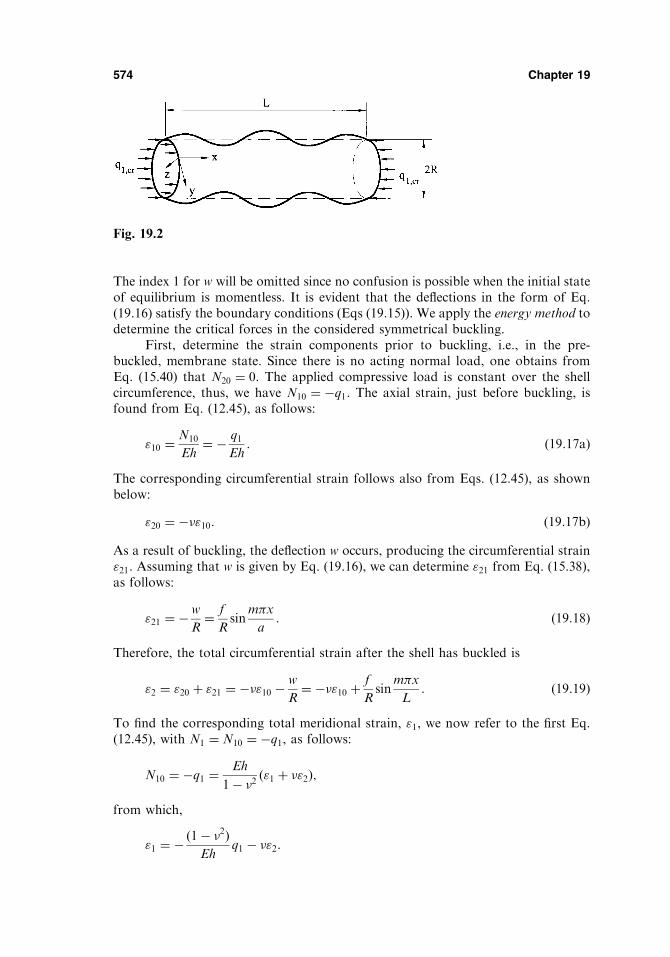
The index 1 for w will be omitted since no confusion is possible when the initial stateof equilibrium is momentless. It is evident that the deflections in the form of Eq.(19.16) satisfy the boundary conditions (Eqs (19.15)). We apply the energy method todetermine the critical forces in the considered symmetrical buckling.

First, determine the strain components prior to buckling, i.e., in the pre-buckled, membrane state. Since there is no acting normal load, one obtains fromEq. (15.40) that N20 ¼ 0. The applied compressive load is constant over the shellcircumference, thus, we have N10 ¼ �q1. The axial strain, just before buckling, isfound from Eq. (12.45), as follows:

"10 ¼N10

Eh¼ � q1

Eh: ð19:17aÞ

The corresponding circumferential strain follows also from Eqs. (12.45), as shownbelow:

"20 ¼ ��"10: ð19:17bÞ

As a result of buckling, the deflection w occurs, producing the circumferential strain"21. Assuming that w is given by Eq. (19.16), we can determine "21 from Eq. (15.38),as follows:

"21 ¼ �w

R¼ f

Rsin

m�x

a: ð19:18Þ

Therefore, the total circumferential strain after the shell has buckled is

"2 ¼ "20 þ "21 ¼ ��"10 �w

R¼ ��"10 þ

f

Rsin

m�x

L: ð19:19Þ

To find the corresponding total meridional strain, "1, we now refer to the first Eq.(12.45), with N1 ¼ N10 ¼ �q1, as follows:

N10 ¼ �q1 ¼Eh

1� �2 ð"1 þ �"2Þ;

from which,

"1 ¼ � ð1� �2ÞEh

q1 � �"2:

574 Chapter 19

Fig. 19.2

Thus, the expressions (19.43) and (19.46) can be applied to cylinders for which Z �2:85 or whose length L > 1:69


p=ffiffiffiffiffiffiffiffiffiffiffiffiffi1� �24

p. Such cylinders are classified as moder-

ate-length cylinders. For short cylinders, for Z less than 2.85, the values of ¼ 0 andm ¼ 1 are to be substituted into Eq. (19.41). For a short and simply supportedcylinder, we obtain

K1 ¼ 1þ 12Z2

�4: ð19:49Þ

The critical stress for cylinders with Z < 2:85 is thus given by

�1;cr ¼K1�

2D

hL2; ð19:50Þ

where K1 is defined by Eq. (19.49). Expression (19.50) indicates that the critical stressof a short cylinder approaches that of a wide laterally unsupported plate as Zapproaches zero or as a simply supported column.

In the foregoing analysis, it was assumed that failure would occur as a result oflocal surface buckling. This assumption is valid only as long as the cylinder is notextremely slender. Long narrow cylinders may become unstable as a result of Euler’scolumn buckling (general or global instability) before the local instability stress isreached, and must therefore be checked for both modes of failure. It has thus beenshown that the buckling mode of an axially loaded cylinder depends on the ratio ofits length to its radius. The local instability occurs for short and moderate-lengthcylinders, whereas a long cylinder buckles as a column. There is a big differencebetween local and general bucklings of short and long cylinders. The buckling of avery long cylinder (Euler’s buckling mode) does not involve surface distortion of thecircular cross section at all. Instead, the member simply behaves like Euler’s column.The local instability largely involves a surface distortion for short cylinders.Intermediate-length cylinders are to be found between these two extremes and repre-sent the majority of actual cylinders. Cylinders of this type buckle by developingsurface distortions in both the longitudinal and circumferential directions, and theircritical stress is given by Eq. (19.46).

19.3.3 Buckling of cylindrical shells under external pressure

Consider the case when a shell is subjected to uniform external pressure of intensity p(Fig. 19.3). Such a type of loading is typical for submarine hulls and shell aircraftengine housings. Also tanks in chemical plants often experience an excessive externalpressure.

The external uniform pressure causes the membrane longitudinal stress �1 andcircumferential stress �2, as well as the bending stresses in a cylindrical shell. Inanalyzing the shell buckling, the circumferential compressive stresses are of greatimportance. If a shell is sufficiently long, then the critical values of the externalpressure p only slightly affect the boundary conditions prescribed on the shelledges. This means that a distortion of the circular cross section will be identicalthroughout the length of the shell. Hence, the buckling analysis of long cylindricalshells can be replaced (for the sake of simplicity) by the analysis of the stability of aring of unit length with the same radius and thickness as for the given shell. Such a


buckling problem was analyzed, for example, in Ref. [2]. The critical value of theexternal pressure is given by

pcr ¼ðn2 � 1ÞEI

R3; ð19:51Þ

where n is the number of half-waves in the circumferential direction. The minimumvalue of pcr is reached when n ¼ 2, i.e.,

pcr:min ¼ 3EI

R3: ð19:52Þ

For long shells, pcr is also given by Eq. (19.52), replacing EI by the flexural rigidity,D ¼ Eh3=12ð1� �2Þ.

If a cylindrical shell subjected to a uniform external pressure is not too long,then its buckling analysis should be carried out with the use of equations of thestructural stability theory, discussed in Sec. 19.2. Assume that the shell edges aresimply supported and there is no bending of the shell. The circumferential stress is�2 ¼ �pR=h. Hence, the action of the transverse pressure p is equivalent to the actionof the compressive circumferential forces, equal to pR. Making use of the homoge-neous equation (19.9) and setting N10 ¼ 0; N20 ¼ �pr; and S ¼ 0 and dividing bothsides by h, one obtains the following equation for the problem under consideration:

D

hr8wþ E

R2

@4w

@x4þ pR

hr4 @2w

@y2

!¼ 0: ð19:53Þ

where r8 � r4ð. . .Þr4ð. . .Þ.One can take the solution of this equation in the form of Eq. (19.34) that

satisfies the prescribed boundary conditions. Substituting the above expression forw into Eq. (19.53), one obtains the following:

D

h

m2�2

L2þ n2

R2

!4

þ E

R2

m4�4

L4� pR

h

m2�2

L2þ n2

R2

!2n2

R2¼ 0; ð19:54Þ

from which

580 Chapter 19

Fig. 19.3

where

qq1 ¼q1R

Eh; pp ¼ p

E

R

h

� �2

; � ¼ m�R

nL; ¼ n2h

R: ð19:64Þ

It is seen that the critical combinations of values qq1 and pp are related to one anotherby a linear relationship. The plot of qq1 vs pp represents some polygon ACDB, asshown in Fig. 19.4. This figure is taken from Ref. [4].

Note that points A and B in this figure correspond to the upper critical valuesof axial compressive load, qq1cr, and external pressure, ppcr, respectively, applied sepa-rately from one another. If we join these points by a straight line, we obtain someintermediate values of qq1 and pp corresponding to the following equation:

qq1qq1cr

þ pp

ppcr¼ 1

or

q1q1cr

þ p

pcr¼ 1 ð19:65Þ

(the superscript 1 that refers to the upper critical loads is omitted in the above andfurther equations, because in the linear buckling analysis only such a critical load canbe obtained).

It is easily seen that Eq. (19.65) determines the critical combination of the axialloads and external pressure conservatively with respect to the polygon. Therefore,this equation can be used as a first approximation in a practical design.

Theoretical investigations and experiments showed that an axial compressiondecreases the value of the external critical pressure, compared with the case when thiscompression is absent. An axial tension increases the value of the external criticalpressure. In turn, an internal pressure increases the value of the axial compressivecritical force.

Also it should be noted that in the shell buckling problems introduced above,the solutions were obtained by assigning the boundary conditions for the deflectionsof the type of Eqs (19.15) on the shell edges, ignoring the in-plane displacementsprescribed also on these edges. The investigations associated with the effect of the in-


Fig. 19.4

w ¼ f sin�x

asin�y

a: ð19:73Þ

The panel is also assumed to have an initial deflection, given by

wi ¼ fi sin�x

asin�y

a: ð19:74Þ

It was shown [10] that the effect of initial imperfections is found to be stronger iftheir shape corresponds to the wave-like behavior of a perfect shell in buckling.

Let us substitute for w and wi from Eqs (19.73) and (19.74) into the second Eq.(19.72). Making in the above equation �2 ¼ 1=R; �1 ¼ 0, one obtains the following:

r2r2� ¼ E ðf 2 þ 2f � f1Þ�4

2a4cos

2�x

aþ cos

2�y

a

� �þ f�2

Ra2sin�x

asin�y

a

" #:

ð19:75ÞA particular solution of this equation, obtained by the method of undeterminedcoefficients, is

�p ¼ Eðf 2 þ 2f � fiÞ32

cos2�x

aþ cos

2�y

a

� �þ Efa2

4�2Rsin�x

asin�y

a: ð19:76Þ

Determine the complementary solution of Eq. (19.75), �h. This solution shouldsatisfy the homogeneous equation r2r2� ¼ 0 and also has to correspond to theprimary membrane forces that exist prior to buckling and are caused by the givenloading q1. We have that N1 ¼ �q1;and N2 ¼ S ¼ 0. Noting that

q1h¼ @2�

@y2;

one obtains the following:

�h ¼ � q1y2

2h: ð19:77Þ

Thus, the general solution of the second Eq. (19.72) is obtained, as follows:

� ¼ Eðf 2 þ 2f � fiÞ32

cos2�x

aþ cos

2�y

a

� �þ Efa2

4R�2sin�x

asin�y

a� q1y

2

2h: ð19:78Þ

Now, let us return to the first Eq. (19.72). We satisfy this equation approximatelyonly in Galerkin’s procedure sense. So, setting p3 ¼ 0; �1 ¼ 0; and �2 ¼ 1=R, weobtainða ða

0

D

hr2r2w� Lðw;wi;�Þ �

1

R

@2�

@x2

" #sin�x

asin�y

adxdy ¼ 0: ð19:79Þ

Substituting for w;wi; and � from Eqs (19.73), (19.74), and (19.78) into the aboveand integrating, we obtain, after some mathematics, the following equation:

Df�4

a2� q1�

2

4ðf þ fiÞ þ

Efha2

16R2� 5

6f þ fi

� �Eh

Rf þ Eh�4

32a2ðf 2 þ 3ffi þ 2f 2i Þf ¼ 0;

ð19:80Þ


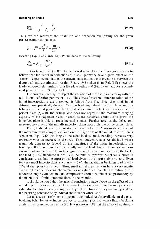
qqð1Þ1;cr ¼

�2

3ð1� �2Þ þk2

�2: ð19:89Þ

Thus, we can represent the nonlinear load–deflection relationship for the givenperfect cylindrical panel as

qq1 ¼ qqð1Þ1 þ �

2

8�2 � 10

3�2k�: ð19:90Þ

Inserting Eq. (19.89) into Eq. (19.88) leads to the following:

qqð2Þ1;cr ¼ qq

ð1Þ1;cr �

200

9�6k2: ð19:91Þ

Let us turn to Eq. (19.83). As mentioned in Sec.19.2, there is a good reason tobelieve that the initial imperfections of a shell geometry have a great effect on thescatter of experimental data of the critical loads and on the discrepancies between thetheoretical and experimental results. Figure 19.6 (taken from Ref. [11]) shows theload–deflection relationships for a flat plate with k ¼ 0 (Fig. 19.6a) and for a cylind-rical panel with k ¼ 24 (Fig. 19.6b).

The curves in each figure depict the variation of the load parameter qq1 with thetotal lateral deflection parameter �þ �i. The curves for several different values of theinitial imperfection �i are presented. It follows from Fig. 19.6a, that small initialdeformations practically do not affect the buckling behavior of flat plates and thebehavior of the flat plate is similar to that of a column. In fact, as in the case of theperfect plate (�i ¼ 0), the critical load does not represent the maximum carryingcapacity of the imperfect plate. Instead, as the deflection continues to grow, theimperfect plate is able to resist increasing loads. Furthermore, as the deflectionsincrease, the curves of the initially imperfect plates approach that of the perfect plate.

The cylindrical panels demonstrate another behavior. A strong dependence ofthe maximum axial compressive load on the magnitude of the initial imperfection isseen from Fig. 19.6b. As long as the axial load is small, bending increases verygradually with an increase in the load. Then, suddenly, at a certain load whosemagnitude appears to depend on the magnitude of the initial imperfection, thebending deflections begin to grow rapidly and the load drops. The important con-clusion that can be drawn from this figure is that the maximum load, i.e., the buck-ling load, q1b as introduced in Sec. 19.2, the initially imperfect panel can support, isconsiderably less that the upper critical load given by the linear stability theory. Evenfor very small imperfections, such as �i ¼ 0:05, the maximum buckling load is only75% of the upper critical load. Thus, small initial imperfections have a very signifi-cant effect on the buckling characteristics of cylindrical panels. The failure of themoderate-length cylinders in axial compression should be influenced profoundly bythe magnitude of initial imperfections in the cylinder.

It should be noted that the general conclusions made above on the effect of theinitial imperfections on the buckling characteristics of axially compressed panels arevalid also for closed axially compressed cylinders. However, they are not typical forthe buckling behavior of cylindrical shells under other loads.

Let us discuss briefly some important theoretical results available on the post-buckling behavior of cylinders subject to external pressure whose linear bucklinganalysis was presented in Sec. 19.3.3. It was shown [4,8] that the effect of nonlinear-


shells, introduced in Sec. 17.3, let us derive the governing differential equations forthe structurally orthotropic circular cylindrical shell. Assume that the stiffeners andshell skin are made of the same isotropic material having the modulus of elasticity Eand Poisson’s ratio �, and that the stiffeners are symmetric with respect to the middlesurface (i.e., K11 ¼ K22 ¼ 0). For this particular case, setting R1 ! 1 and R2 ¼ R,the governing equations of the stiffened cylindrical shells, Eqs (18.63) and (18.66),are reduced to the following form:

D11

@4w

@x4þ 2ðD21 þD33Þ

@4w

@x2@y2þD22

@4w

@y4� 1

R

@2�

@x2¼ p3;

B11

Bs

@4�

@x4þ 1

B33

� 2B12

Bs

� �@4�

@x2@y2þ B22

Bs

@4�

@y4þ 1

R

@2w

@x2¼ 0:

ð19:94Þ

It can be shown that for an unstiffened circular cylindrical shell, D11 ¼ D22 ¼ D;D12 ¼ �D; D33 ¼ Dð1� �Þ; B11 ¼ B22 ¼ B; B12 ¼ �B; B33 ¼ Bð1� �Þ=2;Bs ¼ B2ð1� �2Þ, Eqs (19.94) are reduced to the governing equations of an isotropiccircular cylindrical shells according to the DMV theory. If R ! 1, the first Eq. of(19.94) transforms into Eq. (7.31), derived in Sec. 7.2 for the structurally orthotropicflat plates. Introducing the operators

r4Dð::Þ � D11

@4ð::Þ@x4

þ 2ðD12 þD33Þ@4ð::Þ@x2@y2

þD22

@4ð::Þ@y4

;

r4Bð::Þ �

B11

Bs

@4ð::Þ@x4

þ 1

B33

� 2B12

Bs

� �@4ð::Þ@x2@y2

þ B22

Bs

@4ð::Þ@y4

;

ð19:95Þ

we can rewrite Eqs (19.94) as follows:

r4Dw� 1

R

@2�

@x2¼ p3; r4

B�þ 1

R

@2w

@x2¼ 0: ð19:96Þ

In the buckling analysis problems, p3 is replaced by pðfÞ3 from Eq. (19.8); then the first

Eq. (19.96) becomes

r4Dw� 1

R

@2�

@x2¼ N10

@2w

@x2þN20

@2w

@y2þ 2S0

@2w

@x@y: ð19:97Þ

Consider a structurally orthotropic circular cylindrical shell subjected to uniformaxial compression forces q1. Using Eqs (19.96) and (19.97) and setting N10 ¼ �q1;N20 ¼ S0 ¼ 0, one obtains the following:

r4Dw� 1

R

@2�

@x2þ q1

@2w

@x2¼ 0;

r4B�þ 1

R

@2w

@x2¼ 0:

ð19:98Þ

The Galerkin method can be applied to solving Eqs (19.98). Let us approximate thedeflection w by the following series (the first-order approximation):

w ¼ f sin�x

lxsin�y

ly; ð19:99Þ

592 Chapter 19

where lx and ly are the lengths of the half-waves in the longitudinal and circumfer-ential directions, respectively. Dropping intermediate and lengthy manipulations, wepresent below, following Volmir [4], the final result for the upper critical forcescorresponding to the axisymmetric mode of buckling, when only circumferentialaxisymmetric bulges take place. In this particular case, w ¼ f sin�x=lx and theabove-mentioned critical forces are

qð1Þ1;cr ¼

2

R

ffiffiffiffiffiffiffiffiffiffiffiffiffiD11Bs

B11

s: ð19:100Þ

For an isotropic circular cylindrical shell subjected to compressive forces q1 in thelongitudinal direction, the above expression passes into Eq. (19.30).

Similarly, the stability problem for a cylindrical shell simply supported on itsends and reinforced by closely spaced (at equal distances lx stiffening rings underexternal pressure, can be considered. Assume that the rings are symmetrically placedwith respect to the shell midsurface and that the shell and rings are made of the sameisotropic material, having the modulus of elasticity E and Poisson’s ratio �. For thisparticular case, Eqs (18.48) and (18.50) are simplified to the following form:

B11 ¼ B ¼ Eh

1� �2 ; B12 ¼ B21 ¼ B; K11 ¼ K22 ¼ 0;

B22 ¼ Bþ EAc

lx; B33 ¼ B

1� �2

;

D11 ¼ D ¼ Eh3

12ð1� �2Þ ; D12 ¼ D21 ¼ �D; D22 ¼ Dþ EIclx; D33 ¼ Dð1� �Þ;

ð19:101aÞ

where Ac and Ic are the cross-sectional area and moment of inertia of the ringsabout the tangent to the middle surface. Comparing the rigidities of the cylind-rical shell reinforced by rings (Eqs (19.101a)) and the rigidities of the orthotropiccylindrical shell (Eqs (18.44) and (18.45b)), we can derive the following approx-imate relations for the elastic constants in the reduced structurally orthotropicshell:

E1 ¼ E;E2 ¼ E 1þ Ac

lxh

� �;D1 ¼ D;D2 ¼ Dþ EIc

lx;

�2 ¼ �; �1 ¼�E

E2

;D3 ¼ DG þ �D1 ¼ D;

�1 ¼1

E; �2 ¼

1

E2

; �3 ¼1þ �� E=E2

E:

ð19:101bÞ

Substituting these values into Eqs (19.92) and (19.93) leads to the followingexpression for the critical value of external pressure:


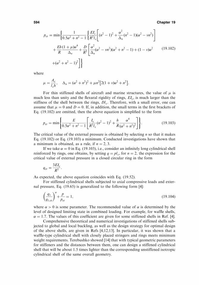
pcr ¼ min1

0:52 þ n2 � 1

EIcR3lx

ðn2 � 1Þ2 þ 2

�n

ðn2 � 1Þð2 � �n2Þ" #

þ Eh

R

ð1þ �Þ4�n

þ D

R3

2

�n

"ð2 � �n2Þð2 þ n2 � 1Þ þ ð1� �Þ2

þð2 þ n2 � 1Þ2��

ð19:102Þ

where

� ¼ Ac

lxh; �n ¼ ð2 þ n2Þ2 þ �n2 2ð1þ �Þ2 þ n2

� �:

For thin stiffened shells of aircraft and marine structures, the value of � ismuch less than unity and the flexural rigidity of rings, EIc, is much larger than thestiffness of the shell between the rings, Dlx. Therefore, with a small error, one canassume that � ¼ 0 and D ¼ 0. If, in addition, the small terms in the first brackets ofEq. (19.102) are omitted, then the above equation is simplified to the form

pcr ¼ minE

0:52 þ n2 � 1

IcR3lx

ðn2 � 1Þ2 þ h

R

4

ð2 þ n2Þ2" #( )

: ð19:103Þ

The critical value of the external pressure is obtained by selecting n so that it makesEq. (19.102) or Eq. (19.103) a minimum. Conducted investigations have shown thata minimum is obtained, as a rule, if n ¼ 2; 3.

If we take ¼ 0 in Eq. (19.103), i.e., consider an infinitely long cylindrical shellreinforced by rings, one obtains, by setting q ¼ plx, for n ¼ 2; the expression for thecritical value of external pressure in a closed circular ring in the form

qcr ¼3EIcR3

:

As expected, the above equation coincides with Eq. (19.52).For stiffened cylindrical shells subjected to axial compressive loads and exter-

nal pressure, Eq. (19.65) is generalized to the following form [4]:

q1q1;cr

� �þ p

pcr¼ 1; ð19:104Þ

where > 0 is some parameter. The recommended value of is determined by thelevel of designed limiting state in combined loading. For example, for waffle shells, ¼ 1:7. The values of this coefficient are given for some stiffened shells in Ref. [4].

Comprehensive theoretical and numerical investigations of stiffened shells sub-jected to global and local buckling, as well as the design strategy for optimal designof the above shells, are given in Refs [4,12,13]. In particular, it was shown that awaffle-type cylindrical shell with closely placed stringers and rings meets minimumweight requirements. Terebushko showed [14] that with typical geometric parametersfor stiffeners and the distances between them, one can design a stiffened cylindricalshell that will be about 1.5 times lighter than the corresponding unstiffened isotropiccylindrical shell of the same overall geometry.

594 Chapter 19

19.6 STABILITY OF CYLINDRICAL SANDWICH SHELLS

Consider a closed cylindrical sandwich shell loaded symmetrically about its middlesurface. The buckling analysis of the sandwich shells includes two modes of buck-ling: a global (or general), associated with bending of the middle surface of the shell;and a local, which is manifested in bending of facing sheets without bending of theshell as a whole. The local bending of face sheets can be modeled by a shell resting onan elastic foundation. In this book, we consider only the global buckling of a sand-wich shell.

The small-deflection theory of the shallow sandwich shells was introduced inSec. 18.4. The governing differential equations (18.78), (7.129), and (18.81) derivedfor the shallow sandwich shells may also be applied to a circular cylindrical sandwichshell if its middle surface is referred to the coordinates x and y measured along theshell generator and arc of its cross section. To apply the above-mentioned equationsfor the stability problems, they should be modified. The value of the transversesurface load p3 in the fifth equation of equilibrium (Eq. 18.78e)) has to be replacedby the value of p

ðfÞ3 according to Eq. (19.8). Thus, Eqs (18.78a–d) remain unchanged,

while Eq. (18.78e), for the buckling problems of the sandwich cylindrical shell, takesthe form

@Q1

@xþ @Q2

@yþN10

@2w

@x2þN20

1

Rþ @

2w

@y2

!þ 2S0

@2w

@x@y¼ 0: ð19:105Þ

The stress resultants–displacements relations have the form of Eqs (18.81). Theconstitutive equations in terms of the moments, shear forces, and deflections are,as follows (see Eqs. (7.129)):

M1 ¼ �D 1

@2w

@x2þ �2

@2w

@y2

!� 1

DQ1

@Q1

@xþ �2DQ2

@Q2

@y

� �" #;

M2 ¼ �D 2

@2w

@y2þ �1

@2w

@x2

!� 1

DQ2

@Q2

@yþ �1DQ1

@Q1

@x

� �" #;

H ¼ �D12

@2w

@x@y� 1

2

1

DQ1

@Q1

@yþ 1

DQ2

@Q2

@x

� �" #;

ð19:106Þ

where

D 1 ¼

D1

1� �1�2; D

2 ¼D2

1� �1�2; ð19:107Þ

and �1; �2;D1;D2; and D12 are the flexural Poisson’s ratios, flexural and twistingstiffness, respectively; DQ1

and DQ2are the transverse shear stiffnesses (see Sec. 7.6).

Let us analyze the compressive buckling of an isotropic, sandwich circularcylindrical shell. For this special case, the above governing differential equationsof the small-deflection sandwich shell theory can be reduced to a single eight-orderdifferential equation in w in the form of Eq. (18.83). Modifying the above equationsto the stability analysis of the sandwich circular plate, we obtain


Dsr4r4wþ 1� Ds

DQ

r2

� �2Ef t

R2

@4w

@x4

!� r4 N10

@2w

@x2þN20

@2w

@y2

"

þ2S0

@2w

@x@y

!#¼ 0;

ð19:108Þ

where Ds and DQ are given by Eqs (18.82).Following Plantema [17], consider the axisymmetric buckling of an infinitely

long, axially compressed isotropic sandwich cylinder. Let the axial compressive loadper unit run be q1. Then, N10 ¼ �q1, N20 ¼ S0 ¼ 0. For axisymmetric buckling, it isobserved that all derivatives of the deflection w with respect to the y coordinatevanish. Thus, Eq. (19.108) is simplified to the following:

Ds

@8w

@x8þ 1� Ds

DQ

@2

@x2

!@4

@x42Ef t

R2wþ q1

@2w

@x2

!¼ 0: ð19:109Þ

A solution of this equation may be represented in the form

w ¼ A sin�x

l; ð19:110Þ

where l is the half-wave length in the axial direction. Substituting the above into Eq.(19.109), we obtain, after some mathematics, the following:

q1 ¼�2Ds

l21þ �

2Ds

l2DQ

!�1

þ 2Ef tl2

�2R2:

With

Ds ¼Ef td

2

2ð1� �2Þthis equation becomes

q1 ¼ Ds

�2

l21þ �

2Ds

l2DQ

!�1

þ 4ð1� �2Þl2�2R2d2

24

35: ð19:111Þ

Find the minimum value of q1 as a function of the continuous variable l. Thecondition @q1=@l ¼ 0 leads to the following relationship:

l2

�2¼ Rd

2ffiffiffiffiffiffiffiffiffiffiffiffiffi1� �2

p � Ds

DQ

: ð19:112Þ

Substitution of the above into Eq. (19.111) gives the following expression for thecritical load:

q1;cr ¼4Ds

ffiffiffiffiffiffiffiffiffiffiffiffiffi1� �2

p

Rd1�Ds

ffiffiffiffiffiffiffiffiffiffiffiffiffi1� �2

p

DQRd

!: ð19:113Þ

596 Chapter 19

The boundary of the domain of this jump corresponds to the case when the diagramppð�Þ has a point of inflection with a horizontal tangent. In so doing, the expressionunder the radical sign must vanish. Thus, a limiting value of k will be of the form

k ¼�2 1þ 1

�

� �2ffiffiffiffiffiffiffiffiffiffiffiffiffiffiffiffiffiffi6ð1� �2Þ

p for � ¼ 3

32k : ð19:124Þ

If we retain four terms in series (19.177), the refined solutions will be obtained. Theyare shown by solid lines in Fig.19.7. It is seen from this figure that the distinctions ofthe refined diagrams from the first-approximation diagrams become perceptible onlyfor ‘‘elevating’’ shells, starting with k ¼ 36, and the refined diagrams give slightlylower upper critical values of pressure. However, the refined diagrams illustrate thechanges in the lower critical loads: in some cases, the loads change sign.

19.8 BUCKLING OF CONICAL SHELLS

Thin conical shells find wide applications in the structures of jet engines, aircrafts,liquid storages, reservoirs, etc. Buckling analysis of conical shells is more compli-cated than the corresponding analysis of cylindrical shells, because of the complexityof the stability governing equations.

We consider below some final results of the linear buckling analysis of inter-mediate-length conical shells subjected to uniform external pressure p, as shown inFig. 19.8. Assume that the shell ends cannot displace at their ends in the directionnormal to the shell midsurface. The criterion of the ‘‘intermediate-length cylindricalshell’’ was introduced in Sec. 19.3. This criterion can be employed for conical shells,too, by replacing R with the mean radius of the parallel circle rm ¼ ðr1 þ r2Þ=2, andby setting L equal to the length of the longitudinal axis of the shell (Fig. 19.8). Forthe above-mentioned shells, n2 > �2, where n is the number of half-waves in thecircumferential direction of the shell and � ¼ �rm=L. Then, the approximate relationfor determining the critical value of the external pressure in a conical shell is


Fig. 19.7

pcr ¼0:855

ð1� �2Þ0:75Eh

L

h

rm

� �1:5

ðcosÞ1:5: ð19:125Þ

For � ¼ 0:3, this relation appears in the form

pcr ¼ 0:92Eh

L

h

rm

� �1:5

ðcosÞ1:5: ð19:126Þ

This expression differs from the corresponding value of critical pressure in cylind-rical shells, Eq. (19.58), by the factor ðcosÞ1:5. Hence, for angles of conicity of2 < 408, pcr, given by Eqs (19.125) or (19.126), will differ from the critical valueof the external pressure, determined for a mean cylinder of length L and havingR ¼ rm, not more than 10%.

The critical values of other loads (axial forces, twisting moments, etc.) appliedto conical shells with an angle not more than 20, can be approximately found fromthe corresponding relations for cylindrical shells by replacing R with rm and settingthe cylindrical shell length equal to the length of the longitudinal axis of the conicalshell.

19.9 BUCKLING OF SPHERICAL SHELLS

The most important stability problem for thin spherical shells is referred to the casewhen they are loaded by external pressure. Such a type of problem is met in radarantenna caps in aircrafts, submarine bulkheads, bottoms of reservoirs, etc. We con-sider here the linear buckling analysis of spherical segments whose rise is comparablewith their radius and closed spherical shells under external pressure. The stabilityanalysis of shallow spherical shells under external pressure was considered in Sec.19.7.

We determine the critical load for a closed spherical shell. It was shown that thecritical stresses for the above shell and for elevated spherical segments under externalpressure are identical [4]. We assume that within the limits of area of local initialbulging, the shell can be considered as a shallow one: therefore, Eqs (17.36) areapplicable. For a spherical shell, the operator r2

kð::Þ ¼ r2ð::Þð1=RÞ, where R is theradius of the middle surface. Thus, Eqs (17.36) for the spherical shell take the form

600 Chapter 19

Fig. 19.8

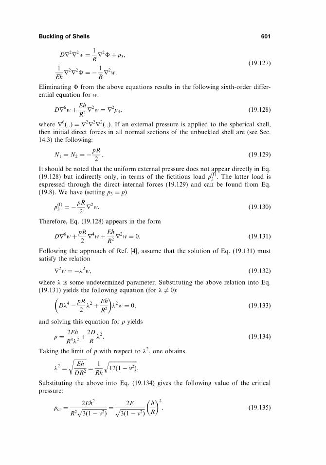
Dr2r2w ¼ 1

Rr2�þ p3;

1

Ehr2r2� ¼ � 1

Rr2w:

ð19:127Þ

Eliminating � from the above equations results in the following sixth-order differ-ential equation for w:

Dr6wþ Eh

R2r2w ¼ r2p3; ð19:128Þ

where r6ð::Þ ¼ r2r2r2ð::Þ. If an external pressure is applied to the spherical shell,then initial direct forces in all normal sections of the unbuckled shell are (see Sec.14.3) the following:

N1 ¼ N2 ¼ � pR

2: ð19:129Þ

It should be noted that the uniform external pressure does not appear directly in Eq.(19.128) but indirectly only, in terms of the fictitious load p

ðfÞ3 . The latter load is

expressed through the direct internal forces (19.129) and can be found from Eq.(19.8). We have (setting p3 ¼ p)

pðfÞ3 ¼ � pR

2r2w: ð19:130Þ

Therefore, Eq. (19.128) appears in the form

Dr6wþ pR

2r4wþ Eh

R2r2w ¼ 0: ð19:131Þ

Following the approach of Ref. [4], assume that the solution of Eq. (19.131) mustsatisfy the relation

r2w ¼ ��2w; ð19:132Þwhere � is some undetermined parameter. Substituting the above relation into Eq.(19.131) yields the following equation (for � 6¼ 0):

D�4 � pR

2�2 þ Eh

R2

� ��2w ¼ 0; ð19:133Þ

and solving this equation for p yields

p ¼ 2Eh

R3�2þ 2D

R�2: ð19:134Þ

Taking the limit of p with respect to �2, one obtains

�2 ¼ffiffiffiffiffiffiffiffiffiffiEh

DR2

r¼ 1

Rh

ffiffiffiffiffiffiffiffiffiffiffiffiffiffiffiffiffiffiffiffiffi12ð1� �2Þ

q:

Substituting the above into Eq. (19.134) gives the following value of the criticalpressure:

pcr ¼2Eh2

R2ffiffiffiffiffiffiffiffiffiffiffiffiffiffiffiffiffiffi3ð1� �2Þ

p ¼ 2Effiffiffiffiffiffiffiffiffiffiffiffiffiffiffiffiffiffi3ð1� �2Þ

p h

R

� �2

: ð19:135Þ


For � ¼ 0:3, we obtain

pcr ffi 1:21Eh

R

� �2

:

The corresponding value of the critical stress, �cr, is

�cr ¼N1;cr

h¼ Eh

R

1ffiffiffiffiffiffiffiffiffiffiffiffiffiffiffiffiffiffi3ð1� �2Þ

p : ð19:136aÞ

or, for � ¼ 0:3

�cr ffi 0:605Eh

R: ð19:136bÞ

Thus, the critical stress of a spherical shell under external pressure is the same as thecritical stress of a closed cylindrical shell under axial uniform compression (see Eq.(19.31b)).

The critical stress given by Eqs (19.136) can be classified as the upper criticalstress, pð1Þcr , for the shell and loading under consideration (see Sec. 19.2). However,numerous experimental investigations showed that the actual critical stresses ofspherical shells under external pressure are far below the values given by Eqs(19.136), obtained on the basis of the linear stability theory. It can be explainedby the fact that the real spherical shells are found to be sensitive to the lightest initialimperfections, just as compressed cylindrical shells discussed in Sec. 19.3.2.Therefore, the buckling analysis of spherical shells should be performed in the frame-work of the nonlinear stability theory. Such a buckling analysis is more complicatedfrom the mathematical and mechanical points of view (for details, see for exampleRef. [4]). We present below only the final results of the nonlinear stability problemfor the spherical shells under external pressure, associated with determining thelower value of the critical pressure, pð2Þcr , which is [4]

pð2Þcr ¼ 0:31Eh

R

� �2

: ð19:137Þ

It is seen that this value is four times less than pð1Þcr .

19.10 DESIGN STABILITY ANALYSIS

Let us summarize the basic theoretical and experimental results of buckling shellanalysis, discussed in the preceding sections. As mentioned previously, there is alarge discrepancy between the analytical predictions of the shell buckling behaviorand the corresponding experimental results. In addition, the scatter of the test datamay be quite large. The major reason for the above discrepancy is the sensitivity ofshell buckling to the initial geometric and loading imperfections, and to deviation inboundary conditions. As a result of these imperfections, as well as the inelasticbehavior of shells in buckling, the critical load of real shells, called the bucklingload in Sec. 19.2, for some shell configurations and loads can be much less than pð1Þcr ,predicted by the linear buckling analysis. It should be noted that application of thegeometrically nonlinear stability theory for determining pð2Þcr , in order to eliminate thediscrepancy between the theoretical and experimental data in the buckling of thin

602 Chapter 19

The critical stress for a short and thin cylinder with length L � 1:22ffiffiffiffiffiffiRh

pfor

simply supported edges, and with L � 2:5ffiffiffiffiffiffiRh

pfor fixed edges, can be determined

from the buckling formula derived previously for a wide flat plate, as follows:

�cr ¼ �Eh2

L2; ð19:140Þ

where � ¼ 0:9 for simply supported and � ¼ 3:6 for fixed shell edges.The alternative buckling stress equations were derived by Donnel and Wan

[10]. They are in good agreement with the relations (19.138) and (19.140).The following approximate equation for the allowable axial compressive stress

in cylindrical shells for elastic buckling was developed in the ASME Code [22] byusing a factor of safety of 10 in Eq. (19.31b):

� ¼ 0:0625Eh

R: ð19:141Þ

For structural steel cylinders, inelastic buckling cannot be readily dealt withusing a plasticity reduction factor. Instead, it is customary to use some empiricalformulas, such as those listed in Refs [22,23].

(b) External pressure

The critical value of external pressure for simply supported cylindrical shells (besidesvery short and very long shells) is given by [4]

pcr ¼ ð0:855Þ Eh2

RLð1� �2Þ0:75ffiffiffiffih

R

r; ð19:142Þ

where the coefficient depends on the ratio R=h, as follows:

R=h . . . . . . . . . 250 500 1000 1500

. . . . . . . . . . . . 0:7 0:6 0:5 0:4

In designing short L � 2:5ffiffiffiffiffiffiRh

p� �, simply supported cylindrical shells under external

pressure, the value of pcr is given by [4]

pcr ¼ 1Eh2

RL; ð19:143Þ

where 1 ¼ 1:8 for all-around pressure and 1 ¼ 3:6 for side pressure.For long, simply supported cylindrical shells ðL > 3:35R

ffiffiffiRh

qÞ, the critical value

of the pressure can be determined from the following relationship:

pcr ¼ 0:275Eh3

R3: ð19:144Þ

The boundary conditions exert some effect on the critical value of the externalpressure. For example, for a cylindrical shell having one pin-connected edge andthe second one fixed, the critical value of external pressure, p cr, is given by [4]

p cr ¼ 0:6pcr; ð19:145Þwhere pcr is the critical value of external pressure for the previously introducedsimply supported cylindrical shell.

604 Chapter 19

An empirical equation developed by the U.S. Navy [20] for the buckling ofcylindrical shells under lateral and axial pressure in the elastic range is given by

pcr ¼2:42E

ð1� �2Þ3=4ðh=2RÞ2:5

L=2R� 0:45ðh=2RÞ0:5� � : ð19:146Þ

For cylindrical shells with large R=h ratios, the above equation can be simplified to

pcr ¼2:42E

ð1� �2Þ3=4ðh=2RÞ2:5L=2R

: ð19:147Þ

19.10.2 Buckling of unstiffened spherical shells under externalpressure

The critical value of external pressure and critical stress is shown below [4]

pcr ¼ Eh2

R2; �cr ¼

Eh

2R; ð19:148Þ

where the coefficient for high-quality manufactured shells and for 250 � R=h �800 is determined by the following formula:

¼ 1

2:368

ffiffiffiffiffiffiffiffiffiffiffiffiffiffiffiffiffiffi100h

R

� �3s

: ð19:149Þ

For the range R=h � 250, according to the recommendations of Ref. [4], ¼ 0:3. If aspherical shell is not manufactured with sufficient accuracy and initial imperfectionsare comparable with its thickness, the coefficient is reduced by about 1.5–2 times.

The following empirical equations for determining the critical stress and thecritical pressure were developed in Refs [17]:

�cr ¼ 0:125Eh

R; pcr ¼ 0:25

Eh2

R2: ð19:150Þ

19.10.3 Buckling of unstiffened conical shells

Conical shells subjected to external pressure can be designed as cylindrical shells withthe effective thickness, he; and efffective length, Le, determined from the followingrelations [24]:

he ¼ h cos; Le ¼L

21þ r1

r2

� �; ð19:151Þ

where h is thickness of the cone, L is the height of the conical shell, and r1 and r2 arethe radii of parallel circles at the top and bottom sections of the truncated cone,respectively.

19.10.4 Stiffened shells

Experimental investigations showed that stiffened shells are less sensitive to overalland local imperfections [12]. Therefore, the critical values of applied loads for suchshells are closer to the theoretically determined values of the upper critical loads


predicted by the linear stability theory. Some empirical equations were developed fordetermining the critical stresses and loads for stiffened shells of various configurationunder axial compression, external pressure, torsion, shear, as well as various loadingcombinations [12,14,19,21]. For example, for the spherical shell with closely andequally spaced stiffeners in two mutually orthogonal directions under external pres-sure, the buckling value of the above pressure is given by [21]

pcr ¼ 0:366EhmR

� �2hbhm

� �3=2

; ð19:152Þ

where hm ¼ hþ A=s is the effective membrane thickness and hb ¼ 12I=sð Þ1=3is theeffective bending thickness; A and I are the area and moment of inertia of thestiffener, s is the spacing between stiffeners.

Local buckling of the spherical shells between the stiffeners must also becon-sidered for large-diameter shells. One such equation is given by

pcr ¼ 7:42Eh3

Rs2: ð19:153Þ

Only a small selection of the recommended design relations for determiningthe critical loads in thin shells has been introduced above. The interested reader isreferred to Refs [4,12,13,14,19–24].

In conclusion, note that in practice one must tend to designing the shell struc-tures whose stability would not depend on occasional and not easily controlledfactors. The basic avenues of designing such shell structures is the use of stiffenedshells, sandwich shells, corrugated shells, etc. In some, the most important cases,sharpened shells are applied.

PROBLEMS

19.1 It follows from Fig. 19.1a that the path of equilibrium for a flat plate is symmetric

about the vertical, p axis, whereas the corresponding path for a shallow shell is non-

symmetrical. Explain the above difference in the buckling behavior of plates and shells.

19.2 Provide a detailed deviation of Eqs (19.3).

19.3 Derive Eqs (19.4) from (19.3) by neglecting all the terms containing prebuckled rota-

tions.

19.4 Derive Eqs (19.9) from Eqs (19.7).

19.5 A water tower support constructed of a long steel piping of 1.0 m diameter is to carry

an axial compression load of 520 kN. Assuming that the supports ends are pin-con-

nected, determine the required thickness of the shell that will prevent this tower sup-

port from buckling. Use L ¼ 2:0m; E ¼ 200GPa; � ¼ 0:3, and a factor of safety (FS)

of 3.5.

19.6 Verify Eq. (19.22)

19.7 A thin steel pipe is subjected to a vacuum pressure of 150 psi. Assuming that the pipe

edges are simply supported, determine the required thickness of the pipe, preventing

the pipe from buckling. Given E ¼ 29,000 psi, � ¼ 0:3, L ¼ 10 ft, R ¼ 2:5 ft, and the

factor of safety (FS) is 3.0.

19.8 Determine the critical stress in a simply supported circular cylindrical panel subjected

to a uniformly distributed compressive forces q1, as shown in Fig. P.19.1. Assume that

the shell edges are simply supported.

Hint: take the deflection w in the form

606 Chapter 19

20

Vibrations of Shells

20.1 INTRODUCTION

The dynamic effects of time-dependent loads on shell structures are quite similarto those discussed in Chapter 9 for plates. Thus, the objectives of the vibrationanalysis of shells, as well the general approach for deriving the shell equationsof motion, remain analogous to the plate vibration analysis introduced in Sec.9.1.

Assume that the state of stress within a shell during vibrations has a char-acter determined by the equations of equilibrium, and the shell middle surfacedeforms according to the same law during vibrations as in the static equilibriumstate. Based on the above, the equations of motion of the vibrating shell can beobtained by applying the D’Alambert principle, just as it was done for vibratingplates – i.e., by adding the inertia forces to given external loads, assigned bycomponents p1; p2; and p3, namely (damping forces are not considered here):

p1 ! p1 � �h@2u

@t2; p2 ! p2 � �h

@2v

@t2; p3 ! p3 � �h

@2w

@t2; ð20:1Þ

where p1; p2; p3; and u; v;w are functions of the Cartesian coordinates of the mid-dle surface and time, � is the mass density of the material, and h is the shellthickness. As for vibrating plates, we distinguish between free vibrations of shells,which occur in the absence of applied loads but are initiated by some initialconditions imposed on the shell, and forced vibrations of shells, which resultfrom the application of time-dependent loads. We consider in this chapter bothtypes of vibrations.

609

20.2 FREE VIBRATIONS OF CYLINDRICAL SHELLS

20.2.1 General

As mentioned in Sec. 9.1, free vibrations deal with some natural characteristics ofshells. These natural vibrations occur at discrete frequencies, depending only on thegeometry and material of the shell. A knowledge of the free-vibration characteristicsof thin elastic shells is important both for our general understanding of the funda-mentals of the shell behavior and for industrial applications of shell structures. Inconnection with the latter, the natural frequencies of shell structures must be knownto avoid the destructive effect of resonance with adjacent rotating or oscillatingequipment (such as jet and reciprocating aircraft engines, electrical machinery, mar-ine turbines and propulsors, etc.).

Since the free vibrations occur in the absence of all external forces(p1 ¼ p2 ¼ p3 ¼ 0), we address the free-vibration analysis of shells with the solutionof homogeneous partial differential equations with homogeneous boundary condi-tions. Let us derive the equations of the free vibrations of thin elastic cylindrical andshallow shells.

20.2.2 Axisymmetric free flexural vibrations of cylindrical shells

Consider the free flexural vibrations of a circular cylindrical shell when the radial wand longitudinal u displacements do not depend on the angular coordinate �, and thecircumferential displacement v is zero. Any cross section of such a shell will be acircular ring, and several half-waves can be placed throughout the shell length, asshown in Fig. 20.1.

The equation of axisymmetrical free vibrations can be obtained from the gov-erning differential equation of the axisymmetrically loaded circular cylindrical shell,Eq. (15.44). One replaces, due to Eq. (20.1), the normal component of the externalloading p3 by the normal component of the inertia forces, and neglects the long-itudinal component of the above forces. Thus, the differential equation of the axi-symmetrically vibrating circular cylindrical shell is found to be

@4w

@x4þ 44w ¼ � �h

D

@2w

@t2; ð20:2Þ

610 Chapter 20

Fig. 20.1

where the deflection w ¼ wðx; tÞ is a function of the x coordinate and time t.The solution of Eq. (20.2) for a simply supported shell of length L, assuming

harmonic equations in time, is sought in the following form:

wðx; tÞ ¼X1n¼1

An sinn�x

Lsin!t; ð20:3Þ

where ! is the frequency of natural vibrations (or natural frequency) of the given shell.It is related to the vibration period T by the relationship ! ¼ 2�=T . Substituting forw from Eq. (20.3) into Eq. (20.2), one obtains

Dn�

L

� �4þEh

R2¼ �h!2;

and the natural frequency ! is given by

!2 ¼ E

�R2ð1þ ��4Þ; ð20:4Þ

where

� ¼ h2

12R2ð1� �2Þ ; � ¼ n�R

L: ð20:5Þ

The value of � for thin shells is small compared with unity. For shells that are notshort, when �4 < 1, the product ��4 can be neglected. Then, the natural frequency ofaxisymmetrical vibrations for all numbers n will coincide with the natural frequencyof axisymmetrical vibrations of a ring or an infinitely long shell. For other shells, notsimply supported at their ends, a solution of Eq. (20.2) will be sought in the follow-ing general form:

wðx; tÞ ¼ WðxÞ sin!t: ð20:6ÞSubstituting the above into Eq. (20.2), we obtain an ordinary fourth-order differ-ential equation inWðxÞ. Its solution will have an analogous form to that discussed inSec. 15.3 if axisymmetrical deformations of a statically loaded circular cylindricalshell are of interest. Satisfying the given boundary conditions, one can obtain – fromthe condition of nontriviality of the above solution – the expression for the naturalfrequencies in axisymmetrically vibrating cylindrical shells. For example, for fixedshell edges, the natural frequency of the first mode of axisymmetrical vibrations (thefundamental natural frequency) is determined from the following equation:

!21 ¼

E

�R21þ � 4:73

R

L

� �4" #

: ð20:7aÞ

The frequency of the second harmonics for the above shell is

!22 ¼

E

�R21þ � 7:83

R

L

� �4" #

: ð20:7bÞ

Since the value of � for thin shells is small, then, as follows from Eqs (20.7), the fixededges of the shell have a low effect on the natural frequencies of vibrations ascompared with the simply supported edges. Similar results will be obtained forother boundary conditions. Hence, the natural frequency of axisymmetrical (long-

Vibrations of Shells 611

itudinally-radial) vibrations of thin and not-short circular cylindrical shells dependsa little on boundary conditions and on the mode of vibrations (for the first mode).

To determine the frequencies of axisymmetric vibrations, the energy method,based on the variational principles (see Sec. 2.6), can also be applied. As shown inSec. 15.3, the axisymmetric bending of a circular cylindrical shell is quite similar tothe bending of a strip-beam of unit width cut off the shell and resting on an elasticfoundation with the foundation modulus k ¼ Eh=R2. The strain energy of such astrip-beam, deflecting by wðxÞ; will be of the form

U ¼ EI

2

ðL0

d2w

dx2

!2

dxþ k

2

ðL0

w2dx; ð20:8Þ

where L denotes the span of the strip-beam. It follows from the above that the strainenergy consists of the strain energy of the strip-beam itself, which is proportional toh3, and the energy of the elastic foundation, which is proportional to h (the shellthickness). If the small value of the strain bending energy (the first term in Eq. (20.8))is neglected, then the maximum value of the strain energy will be equal to thefollowing:

Umax ¼Eh

R2

ðL0

w2dx: ð20:9Þ

The maximum value of the kinetic energy for any mode of free vibrations is given by

Kmax ¼�h!2

2

ðL0

w2dx:

Equating Umax and Kmax, we obtain the following expression for the frequency offree vibrations:

!2 ¼ E

�R2: ð20:10Þ

Hence, under the assumption introduced above (neglecting the bending potentialenergy of a strip-beam in Eq. (20.8)), the frequency of natural radial vibrationsdoes not depend on wmax, i.e., on the vibration mode and boundary conditions. Itis necessary only that a circular cross section is preserved on the shell ends.

In increasing the shell thickness and decreasing its length, the dependence ofvibration frequencies on the mode and boundary conditions becomes more signifi-cant. For cylindrical shells, such a mode of axisymmetric vibrations is possible whenu ¼ w ¼ 0. In this case, points of such shells are displaced in the circumferentialdirection only (i.e., v 6¼ 0); these are torsional vibrations.

20.2.3 Free asymmetric flexural vibrations of circular cylindricalshells

1. Closed cylindrical shells

The differential equations of equilibrium in terms of the displacement componentsfor a circular cylindrical shell are given by Eqs (15.7)–(15.9). According to theDonnel–Mushtari–Vlasov (DMV) theory, they can be simplified by dropping thebending terms in the operators l23 and l32 that are proportional to h2=R2 (see Eqs

612 Chapter 20

Since the number of m may be an integer only, then, after determining m from Eq.(20.17), it should be taken to be equal to the nearest integer. The smallest naturalfrequency corresponds to this integer. The second derivative of � with respect to mwill be positive; therefore, Eq. (20.17) defines a minimum.

Example 20.1

For a simply supported closed cylindrical shell of radius R ¼ 17 cm and of lengthL ¼ 54 cm, find the number of half-waves in the circumferential direction and theminimum natural frequency. Use the following geometric and mechanical para-meters of the shell: h ¼ 0:08 cm; � ¼ 0:3; E ¼ 200GPa, and � ¼ 0:3:

Solution

For the given geometric and mechanical shell parameters, we can find thata2 ¼ 0:18 10�5, � ¼ 1, and T1 ¼ 0:9. Substituting the above data into Eq.(20.17), gives m ¼ 5:1. Hence, the minimum natural frequency of predominantlytransverse vibrations, !min, takes place for five half-waves or for 10 nodal pointsplaced over the circumference of the shell cross section. The value of ! is found fromEq. (20.15) for m ¼ 5. The relationship between the frequency and m is shown inFig. 20.2.

Figure 20.3 illustrates the relationship of the frequency for any fixed value of mfrom the shell length, L. It is seen that the frequency decreases as the length of theshell increases. However, starting from some length L , the frequency becomes aconstant and practically coincides with the frequency determined for a shell havingfree edges or for a shell of an infinite length when the shell experiences only bendingwithout stretching of the middle surface.

If a shell is not too short (L > R), then the natural frequency is virtuallyindependent of the boundary conditions and it is possible to determine this fre-quency for a shell with any, say simply supported, boundary conditions.

The strain energy of a shell of any geometry is given by Eq. (12.51). The kineticenergy of a vibrating shell is of the following form:

K ¼ �h

2

ð ðA

@u

@t

� �2

þ @v

@t

� �2

þ @w

@t

� �2" #

ABdd: ð20:18Þ


Fig. 20.2

The functions �mn andWmn must satisfy the prescribed boundary conditions on shelledges x ¼ 0; a and y ¼ 0; b. It is convenient to assign the above functions in the formof the product of two functions, each of which depends upon only one independentvariable, i.e.,

�mn ¼ XnðxÞYmðyÞ; Wmn ¼ �nðxÞmðyÞ:The functions Xn;Ym;�n; and m are chosen such that they would satisfy the givenboundary conditions on the corresponding shell edges. It is convenient to employ theso-called fundamental beam functions [1] as the above-mentioned approximatingfunctions. The Galerkin equations (Eqs (6.39)) for free-vibration analysis of shallowshells can be represented in the following form:ð ð

A

Dr2r2w� r2k�þ �h @

2w

@t2

!Wijdxdy ¼ 0;

ð ðA

r2r2�þ Ehr2kw

� ��ijdxdy ¼ 0:

ð20:24Þ

Substituting for w and � from Eqs (20.23) into the above and evaluating the inte-grals, we obtain a system of homogeneous algebraic equations in Amn and Bmn.Equating the determinant of the above system of equations to zero results in thefollowing characteristic equation for determining the natural frequencies:

!2mn ¼

1

�hDJ4J5

þ EhJ2J3J1J5

� �; ð20:25Þ

where,

J1 ¼ð ð

A

XnYmr2r2ðXnYm

� �dxdy;

J2 ¼ð ð

A

XnYm m

@

@xð�2� 0

nÞ þ�n

@

@y�1

0m

� �� dxdy;

J3 ¼ð ð

A

�nm Ym

@

@xð�2X 0

nÞ þ Xn

@

@yð�1Y 0

mÞ� �

dxdy;

J4 ¼ð ð

A

�nmr2r2�nmdxdy; J5 ¼ð ð

A

�2n

2mdxdy:

ð20:26Þ

In choosing Xn;Ym;�n; and m, it is important to assign orthogonal function,whose second and fourth derivatives also possess orthogonality properties. In thiscase, an infinite system of the homogeneous linear algebraic equations with aninfinite number of equations is separated down into a system consisting of thepair of equations in Amn and Bmn for each pair of the numbers m and n.

2. The Rayleigh–Ritz method

According to the Rayleigh–Ritz method, natural frequencies of free vibrations ofshallow shells are determined from the condition of a minimum of the sum of thepotential and kinetic energies of the shell. The strain energy of a shallow shell is givenby Eq. (17.50) and the kinetic energy for the above shallow shell can be representedby Eq. (20.18), if we put A ¼ B ¼ 1; ¼ x; and ¼ y. If the membrane inertia forces

620 Chapter 20

are neglected compared with the transverse inertia forces, then we obtain, from Eq.(20.18), the following expression for the kinetic energy of a shallow shell:

K ¼ �h

2

ð ðA

@w

@t

� �2

dxdy: ð20:27Þ

If a shell is undergoing harmonic vibrations, then a maximum value of the kineticenergy is given by the following expression:

Kmax ¼�h!2

2

ð ðA

w2dxdy: ð20:28Þ

Assume that the stress function � and deflection w of the shell are approximated bythe expressions (20.23). The conditions of the minimum of the Rayleigh’s fractiongives

@

@Amn

Umax � !2Kmax

� � ¼ 0;@

@Bmn

Umax � !2Kmax

� � ¼ 0; ð20:29Þ

from which the characteristic equation for determining the natural frequencies isobtained.

Example 20.3

Determine the natural frequency of free vibrations of a shallow, simply supportedshell of a double positive curvature. Assume that the shell is a rectangular in a plane,as shown in Fig. 17.6, and �1 ¼ 1=R1 ¼ const; �2 ¼ 1=R2 ¼ const.

Solution

The simply supported boundary conditions on the shell edges are of the form

w ¼ v ¼ M1 ¼ N1 ¼ 0x¼0;a

; w ¼ u ¼ M2 ¼ N2 ¼ 0y¼0;b

: ðaÞLet us approximate the stress function � and deflection surface w by the followingseries:

� ¼X1m¼1

X1n¼1

Amn sin �nx sin�my sin!t;

w ¼X1m¼1

X1n¼1

Bmn sin �nx sin�my sin!t;

ðbÞ

where �n ¼ n�=a; �m ¼ m�=b. It can be shown that the expressions for � and w inthe form of Eqs (b) satisfy the boundary conditions (a). Substituting the expressions(b) into Eqs (20.22), we obtain the homogeneous system of linear algebraic equationsin Amn and Bmn. To obtain a nontrivial solution of this system, it is necessary toequate its denominator to zero. Expanding the above determinant, one obtains

!2mn ¼

1

�hDð�2n þ �2

mÞ2 þEh

�2nR2

þ �2m

R1

� �2

ð�2n þ �2mÞ2

26664

37775: ðcÞ


For a cylindrical, simply supported shallow shell, Eq. (c) takes the following form(R1 ¼ 1;R2 ¼ R ¼ const):

!2mn ¼

1

�hDð�2n þ �2

mÞ2 þEh

R2

�4n

ð�2n þ �2mÞ2

" #: ðdÞ

Equations of a minimum @!2mn=@�n ¼ 0 for a fixed value of �m and @!2

mn=@�m ¼ 0 fora fixed value of �n have no real roots, which shows the monotonic character of thevariation of !2

mn as a function of �n and �m. Thus, the frequency of the fundamentalmode, or the lowest natural frequency of free vibrations of a given shallow, simplysupported shell, corresponds to one half-wave in the x and y directions, i.e.,m ¼ n ¼ 1.

20.5 FREE VIBRATIONS OF STIFFENED SHELLS

The analytical solution of free-vibration problems of stiffened shells presents con-siderable difficulties. Consider the free vibrations of a cylindrical shell reinforced bytransverse rings (collars). The method of an approximate analysis of flexural vibra-tions of such a shell depends on the ratio between the flexural stiffnesses of the ring(in its own plane) and the shell itself. If the shell stiffness Dmultiplied by the distancebetween the rings, lx, is significantly less than the flexural stiffness of the ring, EIr,then the natural frequencies can be found from Eqs (20.4) and (20.15), assumingL ¼ lx. If the value of D � lx is significantly larger than EIr then to determine thenatural frequency of flexural vibrations of the stiffened shell, the stiffness of the ringscan be uniformly distributed over the shell and the latter is considered as structurallyorthotropic, i.e., having different flexural stiffnesses in the longitudinal and trans-verse directions (see Sec. 18.3.2). In the circumferential direction, such a shell willhave the flexural stiffness equals to Dþ EIr=lx, where Ir is the moment of inertia ofthe ring cross section with joined segment of the shell (of length lx) about thecommon axis x of bending of this combined section.

Expression (20.15), for the structurally orthotropic cylindrical shell, can bewritten in the following form:

!2 ¼ 1

�hR2

�4Ehþ ðDþ EIr=lxÞR2 ð�2 þm2Þ4

ð�2 þm2Þ2 þm2: ð20:30Þ

The relation (20.30) is valid if the modulus of elasticity of the shell material differsslightly from the modulus of elasticity of the ring material. If the moduli of elasticityof the shell and ring differ significantly, then the relation (20.15) must be trans-formed, as follows:

!2 ¼ B

MMR2

ð1� �2Þ�4 þ ðDþ ErIr=lxÞBR2 ð�2 þm2Þ4

m2 þ ð�2 þm2Þ2 ; ð20:31Þ

where

B ¼ Esh

1� �2sis the extensional stiffness of the shell at a section of unitlength;

622 Chapter 20

Es and �s are the modulus of elasticity and Poisson’s ratio of theshell material;

MM ¼ �shþAr�rlx

is a shell mass referred to an area of the shell middlesurface;

Ar is the ring’s cross-sectional area;�s and �r are the mass densities of the shell and ring materials,

respectively;

D ¼ Esh3

12ð1� �2s Þþ ErIr

lx

is the flexural stiffness of the stiffened shell (see Eqs(18.50)); and

Er is the modulus of elasticity of the ring material.

All the above relations and equations of free vibrations have been derived forunloaded shells. However, it is known that the natural frequencies of free vibrationsdepend on the character and value of applied static loading, such as the normalsurface pressure, axial force, torque, etc. Let us discuss first an influence of thesestatic loads on the natural frequencies of closed unstiffened circular cylindrical shells.Assume that the shell is simply supported on its edges. The governing differentialequations of free vibrations of such shells will be analogous to those of Eqs (20.11),with an addition of terms depending on the given static loading. Dropping theintermediate mathematics associated with deriving the above equations (these deri-vations are quite similar to those carried out in Sec. 20.2.3), we give only the finalresults. The natural frequency of free vibrations of a circular, simply supportedcylindrical shell subjected to a combined static loading is

� ¼ �0 þð�2 þm2Þ2 1ðm2 � 1Þ þ 2�

2 � 2 3�m� �m2 þ ð�2 þm2Þ2 ; ð20:32Þ

where

�0 ¼ð1� �2Þ�R2

E!20 ¼

ð1� �2Þ�4 þ a2ð�2 þm2Þ4m2 þ ð�2 þm2Þ2 ; ð20:33Þ

!0 is the natural frequency of free vibrations of the unloaded shell, and

1 ¼pRð1� �2Þ

Eh; 2 ¼

N1ð1� �2ÞEh

; 3 ¼Hð1� �2Þ2�R2Eh

; ð20:34Þ

where p is the difference between the normal internal and external pressure, N1 is anaxial tension force, and H is a torque. Thus, it is seen from the expression (20.32)that the presence of the internal pressure and axial tensile force increases the naturalfrequencies of free vibrations in comparison with the corresponding natural frequen-cies of an unloaded shell. An application of the torque decreases the natural fre-quencies of free vibrations corresponding to certain wave numbers m and n.

If the value of m2 in the denominator of Eq. (20.32) is neglected (which corre-sponds to neglecting the membrane internal forces in the vibration equations), thenthe expression for determining the natural frequencies in statically loaded shells issimplified to the following:

� ¼ �0 þ 1ðm2 � 1Þ þ 2�2 � 2 3�m: ð20:35Þ


The external load applied to the shell is also extended into the following series:

p3ðx; y; tÞ ¼ sin�tX1m¼1

X1n¼1

Cmn sin �nx sin�my; ð20:41Þ

where

Cmn ¼4

ab

ð ðA

p3ðx; yÞ sin �nx sin�mydxdy

and

�n ¼n�

a; �m ¼ m�

b: ð20:42Þ

Substituting Eqs (20.40) and (20.41) into Eqs (20.39), we obtain, after some mathe-matics, the following:

Bmn

Ehðk2�2n þ k1�2mÞ2

ð�2n þ �2mÞ2

þDð�2n þ �2mÞ2 � �h�2

" #¼ Cmn: ð20:43Þ

Taking into account expression (c) of Example 20.3 for determining the naturalfrequencies of free vibrations, Eq. (20.43) can be rewritten as follows:

Bmn ¼1

�h

Cmn

ð!2mn ��2Þ : ð20:44Þ

Then, the amplitude of the forced vibrations is determined as follows:

w ¼ 1

�h

X1m¼1

X1n¼1

Cmn

!2mn ��2

; ð20:45Þ

where !mn, the frequency of the natural vibrations of the shallow shell, is given byEq. (c) of Example 20.3.

When the frequency of the forced vibrations, �, coincides with one of thenatural frequencies, a resonance occurs (w ! 1). If � is small compared with!mn, then the deflections will correspond to the case of static loading, i.e.,

BBmn ¼1

�h

Cmn

!2mn

: ð20:46Þ

Let us introduce the dynamic coefficient �, as the ratio of Bmn=BBmn. Using theexpressions (20.44) and (20.46) for the coefficients in the above ratio, we obtain

� ¼ 1

1��2=!2mn

: ð20:47Þ

Let us now consider some special classes of dynamic loading applied to the shallowshell.

1. Uniform surface loading p sin�tFor this type of dynamic loading,

Cmn ¼16p

�2mn; m ¼ 1; 3; 5; . . . ;1; n ¼ 1; 3; 5; . . . ;1;


This chapter contains only some general information about the dynamicresponse of thin shells. The interested reader is referred to Refs [2–5] for additionalreading.

PROBLEMS

20.1 Determine the fundamental natural frequency of the axisymmetric radial free vibra-

tions of a circular cylindrical shell of length L and radius R for the two types of

boundary conditions at the shell ends x ¼ 0 and x ¼ L: (a) the fixed edges and (b)

the simply supported edges. Let R ¼ 0:5m; h ¼ 8mm; L ¼ 4R. The shell is made of

steel.

20.2 Investigate the variation of frequency of free radial vibrations of a simply supported

open circular cylindrical shell (see Fig. 20.4) from its length L. Take the geometric

parameters of the shell in the transverse direction from Example 20.2. Let the shell

length L ¼ 6:0; 10:0; . . . ; 54m with the step of 4.0 m.

Hint: Use Eq. (b) in Example 20.2 for your calculations and take n ¼ 1;

m ¼ 1; 2:3; 4; 5.20.3 Consider a shallow cylindrical shell having a square plan with sides a a. Investigate

an influence of the shell shallowness f =a on the frequencies of free vibrations. Take in

your calculations n ¼ 1;m ¼ 1; 2 in the series expansions. Use the following geometric

and mechanical parameters of the shell: a ¼ 16m; h ¼ 6 cm; E ¼ 15GPa; � ¼ 0:15;and � ¼ 2400 kg=m3. Confine your analysis to the following range: 1/20� f =a � 1=8.

20.4 Calculate the lowest frequency of free vibrations of a spherical shallow shell on a

square plan. Assume that the shell is simply supported on its edges. Let a ¼ 10m; f ¼0:3m; E ¼ 210GPa, � ¼ 2300 kg=m3; � ¼ 0:3; h ¼ 0:1m; and R ¼ 85m.

20.5 Calculate the lowest frequency of free vibrations of a shallow shell of double curvature

on a rectangular plane (Fig. 17.6). The shell is simply supported on its ends. Let a ¼20m; b ¼ 20m, h ¼ 10 cm; f ¼ 4m; R1 ¼ 25m; R2 ¼ 42m; E ¼ 22GPa; and

� ¼ 0:15.20.6 Determine the amplitude of forced vibrations of a cylindrical shell loaded by a con-

centrated harmonic force P sin�t applied at a point with the coordinates 1 and 1.Assume reasonable values for any additional properties and parameters required.

Hint: Replace the given concentrated force by a uniform load q distributed over a small

portion of a cylindrical surface with sides � and , so that q ¼ P=4R2� .20.7 Calculate the amplitude of the forced vibrations of a spherical shallow shell subjected

to a uniformly distributed load p ¼ p0 sin�t. Take as the dimensions of the shell the

frequencies of free vibrations from Problem 20.5. Use p0 ¼ 0:8 kN=m2 and � ¼ 60 s�1.

REFERENCES

1. Vlasov,V.Z., General Theory of Shells and Its Application in Engineering (English trans),

NASA TT F-99, Washington, DC, April 1964.

2. Kraus, H., Thin Elastic Shells, John Wiley and Sons, New York, 1967.

3. Flugge, W., Statik and Dynamik der Schalen, Springer-Verlag, Berlin, 1962.

4. Nowacki, W., Dynamics of Elastic Systems, John Wiley and Sons, New York, 1963.

5. Leissa, A.W., Vibration of Shells, NASA SP-288, Washington, DC, 1973.


Appendix A

Some Reference Data

629

Appendix B

Fourier Series Expansion

B.1 DIRICHLET’S CONDITIONS

A function f ðxÞ defined in the interval �� x � � can be expanded into a trigono-metric series of the type

f ðxÞ ¼ a02þX1k¼0

ak cos kxþ bk sin kxð Þ; ðB:1Þ

provided that:

(a) f ðxÞ has a finite number of jumps discontinuity points in the given inter-val and the limiting finite values of the function exist from the right,f ðx1 þ 0Þ, and from the left, f ðx1 � 0Þ at the above points;

(b) the finite limiting values of f ðxÞ exist at the interval ends, i.e., at pointsf ð�� 0Þ and f ð�þ 0Þ; and

(c) f ðxÞ has a finite number of maximum and minimum in the given intervalð��; �Þ.

B.2 THE SERIES SUM

If Dirichlet’s conditions are satisfied and the coefficients a0; ak; and bk are found (seebelow), then the Fourier series have a sum that is equal to

(a) the given function f ðxÞ at any point of continuity inside the interval��;þ�;

(b) the arithmetic mean of limiting values of f ðxÞ from the right and from theleft from points of the discontinuity jump, i.e., 1

2f ðx1 þ 0Þ þ f ðx1 � 0Þ½ � at

discontinuity points; and(c) the arithmetic mean of limiting values, i.e., 1

2f ð�� 0Þ þ f ð�þ 0Þ½ � on both

end points of the interval (i.e., at points ��;þ�).

635

B.3 COEFFICIENTS OF THE FOURIER SERIES

These coefficients are evaluated by multiplying both parts of the equality (B.1) bycos kxdx and sin kxdx sequentially, and integrating in the limits ��;þ�, i.e.,

a0 ¼1

�

ð��

f ðxÞdx; ak ¼1

�

ð��

f ðxÞ cos kx; bk ¼1

�

ð��

f ðxÞ sin kxdx: ðB:2Þ

If f ðxÞ has discontinuity jumps for x1; x2; . . . ; xs then calculating the above coeffi-cients,

ak ¼1

�

ðx1��

f ðxÞ cos kxdxþ 1

�

ðx2x1

f ðxÞ cos kxdxþ . . .þ 1

�

ð�xs

f ðxÞ cos kxdx;

bk ¼1

�

ðx1��

f ðxÞ sin kxdxþ 1

�

ðx2x1

f ðxÞ sin kxdxþ . . .þ 1

�

ð�xs

f ðxÞ sin kxdx:

B.4 MODIFICATION OF RELATIONS FOR THE COEFFICIENTS OFFOURIER’S SERIES

(a) A given function f ðx Þ is either even or odd

For even function f ðxÞ; the Fourier expansion coefficients are

ak ¼2

�

ð�0

f ðxÞ cos kxdx; bk ¼ 0:

For odd function f ðxÞ; the Fourier expansion coefficients are given by

ak ¼ 0; bk ¼2

�

ð�0

f ðxÞ sin kxdx:

The Fourier expansions for the above two cases will be of the following form:

– for even function (f ð�xÞ ¼ f ðxÞÞ:a02þX1k¼1

ak cos kx:

– for odd function (f ð�xÞ ¼ �f ðxÞ)X1k¼1

bk sin kx:

(b) A function f ðx Þ is defined in the interval �l;þl .

Then,

ak ¼1

l

ðl�l

f ðxÞ cos k�xldx; bk ¼

1

l

ðl�l

f ðxÞ sin k�xl

dx: ðB:3Þ

(c) A given function f ðx Þ is defined in the interval from 0 to 2� (half-rangeexpansion)

Then, in this case, the Fourier expansion coefficients are given by:

636 Appendix B

a0 ¼1

2�

ð2�0

f ðxÞdx; ak ¼1

�

ð2�0

f ðxÞ cos kxdx; bk ¼1

�

ð2�0

f ðxÞ sin kxdx:

(d) A function f ðx Þ is defined in the interval 0; l

Such a function can be expanded into the Fourier series either in sine or cosine. Theexpansions and their coefficients in these cases are:

– expansions in cosines (for even functions)

f ðxÞ ¼ a02þX1k¼1

ak cosk�x

l; ak ¼

2

l

ðl0

f ðxÞ cos k�xldx: ðB:4aÞ

– expansions in sines (for odd functions)

f ðxÞ ¼X1k¼1

bk sink�x

l; bk ¼

2

l

ðl0

f ðxÞ sin k�xl

dx: ðB:4bÞ

B.5 THE ORDER OF THE FOURIER SERIES COEFFICIENTS

Let a function f ðxÞ, defined on the interval ��;þ�, have discontinuities at pointsx01; x

02; . . . ; x

0s . One of the end points, for instance �, should be referred to disconti-

nuity points if the limiting values f ð�þ 0Þ and f ð�� 0Þ are different. For the sake ofnotation symmetry, we designate that latter point by x0sþ1 ¼ �. Let �0i denote a jumpof f ðxÞ at point x0i , so that

�0i ¼ f ðx0i þ 0Þ � f ðx0i�0Þ:The coefficients of the Fourier series will be of the form

an ¼1

�

ðx0i��

f ðxÞ cos nxdxþ 1

�

ðx02x01

f ðxÞ cos nxdxþ . . .þ 1

�

ð�x0s

f ðxÞ cos nxdx:

ðB:5ÞFor example, let f ðxÞ be defined in the form (Fig. B.1)

f ðxÞ ¼ 0 �� x � 0;

f ðxÞ ¼ 1 0 � x � �:

In this case, we have two discontinuities, as follows:

x ¼ 0 �01 ¼ 1

x ¼ � �02 ¼ �1

Fourier Series Expansion 637

Fig. B.1

fmn ¼4

ab

ða0

ðb0

f ðx; yÞ sinm�xa

sinn�y

bdxdy: ðB:17Þ

This agrees with Eq. (3.17) of Sec. 3.3, which was derived differently. Similarly, theresults can be obtained for cosine series or for series having both cosines and sines.

B.7 SHARPENING OF CONVERGENCE OF THE FOURIER SERIES

The following efficient method for sharpening of the convergence of the Fourierseries was proposed by Krylov [A.1].

Let a function f ðxÞ have some discontinuity points in a defined interval. Weselect such a function F0ðxÞ that has the same discontinuity points and jumps as thegiven function. Then, the difference f1ðxÞ ¼ f ðxÞ � F0ðxÞ will have no jumps and,hence, f1ðxÞ will have the Fourier coefficients of the order of 1=n2. Similarly, afunction f 0ðxÞ (the prime notation indicates here the first derivative of the functionwith respect to x) can be treated by letting

f 0ðxÞ ¼ f 01 ðxÞ þ F 0

0ðxÞ ¼ f2ðxÞ þ F1ðxÞwhere F1ðxÞ is some linear function with the same jumps as f 0ðxÞ. Analogously,

f 00ðxÞ ¼ f 02 ðxÞ þ F 0

1ðxÞ ¼ f3ðxÞ þ F2ðxÞ:Expanding this process as long as desired, one can obtain in remainder a Fourierseries with coefficients of any order of smallness.

The present section contains only general information about the Fourier series.The interested reader is referred to Refs [A.2–A.4].

REFERENCES

A.1 Krylov, A.N., Collected Works, vol. 3, parts 1 and 2, Academy of Sciences of the USSR,

Moscow, 1949 (in Russian).

A.2 Churchill, R.V., Fourier Series and Boundary Value Problems, McGraw-Hill, New York,

1960.

A.3 Wylie, C.R., Advanced Engineering Mathematics, McGraw-Hill, New York, 1960.

A.4 Kantorovich, L.V., and Krylov, V.I., Approximate Methods of Higher Analysis, John

Wiley and Sons, New York, 1958.

640 Appendix B

Appendix C

Verification of Relations of the Theoryof Surfaces

C.1 GEOMETRY OF SPACE CURVES

The equation of a three-dimensional curve l can be represented in the Cartesiancoordinate system (X;Y; and Z) by the following one vector equation:

rð�Þ ¼ Xð�Þiþ Yð�Þjþ Zð�Þk; ðC:1Þwhere r is a position vector from the origin of the coordinate system to a point ofinterest and � is some parameter. If Xð�Þ;Yð�Þ; and Zð�Þ are single-valued andcontinuous functions of the parameter �, then we will insure that a given value ofthat parameter defines only one point on the space curve. For example, an arc lengths, measured along the space curve from some origin, can be chosen as such a para-meter. In this case, the vectorial equation (C.1) can be written in the following form:

r ¼ rðsÞ: ðC:2ÞConsider a typical point M and a neighboring point N on the curve l. The positionvectors of those points are r and rþ�r, respectively (Fig. C.1). It is seen from thisfigure that the difference of the two vectors, �r, is depicted by a vector whosemagnitude and direction coincide with the chord, joining the points M and N.When N ! M, the direction of �r approaches the direction of the tangent to thecurve at point M and its length to the arc length between the above points, �s.Hence, in the limit (when �s ! 0), we have

dr ¼ tds;

where t is the unit tangent vector directed along the tangent to the curve l at pointM.Thus, the unit tangent vector to the curve at a point of interest is given by

t ¼ dr

ds; ðC:3Þ

The definition of a curvature of a plane curve was given in Sec. 11.2. Now we reworkthis definition in a vector form for a space curve.

641

Let tM and tN be the two unit tangent vectors at neighboring points M and N,respectively. A change �t in the vector t as we move from point M to point N on thesurface is shown in Fig. C.2.

The vector �t lies in a plane passing through point M and the vectors tM andtN . This plane is called the osculating plane. The length of the vector �t approachesthe value

�tj j ¼ �� ¼ �s

�:

As one goes to the limit, for �s ! 0, one obtains

dt

ds¼ v

�¼ �v; ðC:4Þ

where � is the radius of curvature and �v (� ¼ 1=�) is the curvature vector at point Mof the curve l. Differentiating the identity t

2 ¼ 1 with respect to s, one obtains

642 Appendix C

Fig. C.1

Fig. C.2

form of the surface. To do this, let us calculate the curvature of the curve l, assignedby Eq. (C.6). According to Eq. (C.5), we have

v

�¼ d2r

ds2¼ d

ds

@r

@

d

dsþ @r

@

d

ds

� �¼ @r

@

d2

ds2þ @r

@

@2

@s2þ @2r

@2d

ds

� �2

þ 2@2r

@@

@

@s

d

dsþ @2r

@2d

ds

� �2

:

ðC:7Þ

As mentioned in Sec. C.1, the curvature vector �v is directed along the principalnormal to that curve l in the osculating plane S. Let us project that vector on thedirection of the normal to the surface, given by the unit vector e3, at a point M. Forthis purpose, both sides of the expression (C.7) are multiplied by e3. In doing so, takeinto account that

v

�� e3 ¼ cos �

1

�;

@r

@� e3 ¼ Ae1 � e3 ¼ 0;

@r

@� e3 ¼ Be2 � e3 ¼ 0;

where � is an acute angle between the unit normal vectors to the surface, e3, and tothe curve, v (see Fig. C.3), respectively. As a result of this scalar multiplication, weobtain

cos �

�¼ 1

ds2b11d

2 þ 2b12ddþ b22d2

� �: ðC:8Þ

The term in the parentheses on the right-hand side of Eq. (C.8) represents the secondquadratic form of the surface introduced in Sec. 11.3 (see Eq. (11.18)) and thecoefficients of that form, bik ði; k ¼ 1; 2Þ are given by Eqs (11.17).

It follows from Eq. (C.8) that, among all curves passing through a point ofinterest, a curve whose principal normal, defined by the unit vector v, coincides withthe normal to the surface, defined by the unit normal vector e3, has the smallestcurvature (because in this case, cos � ¼ 1). As mentioned in Sec. 11.2, such a curve isobtained at the intersection of the given surface by a plane passing through a normalto that surface and is referred to as a normal section. The curvature of such a normalsection, �n, is defined by

�n ¼ 1

R¼ b11

d

ds

� �2

þ2b12d

ds

d

dsþ b22

d

ds

� �2

: ðC:9Þ

According to Eq. (C.7), a curvature of any another plane section, �, that makes anangle � with the normal section and has the common tangent with the latter, is of thefollowing form:

� ¼ �n1

cos �: ðC:10Þ

This expression relates the curvature � of any inclined section of the surface to thenormal curvature, �n.

The coefficients of the second quadratic form are given by the relations (11.17)in terms of the curvilinear coordinates and . Substituting the expressions (11.4)and (11.24) into Eqs (11.17), we obtain, after some mathematics, the expressions forthe coefficients bik ði; k ¼ 1; 2Þ in terms of the Cartesian coordinates as follows:

644 Appendix C

b11 ¼1

!

@2X@2

@2Y@2

@2Z@2

@X@

@Y@

@Z@

@X@

@Y@

@Z@

; b22 ¼

1

!

@2X@2

@2Y@2

@2Z@2

@X@

@Y@

@Z@

@X@

@Y@

@Z@

;

b12 ¼1

!

@2X@@

@2Y@@

@2Z@@

@X@

@Y@

@Z@

@X@

@Y@

@Z@

; ðC:11Þ

where

! ¼ffiffiffiffiffiffiffiffiffiffiffiffiffiffiffiffiffiffiffiffiffiffiffiffia11a22 � a212

q: ðC:12Þ

It was mentioned in Sec. 11.3 that the directions of principal curvatures areorthogonal. To prove this, it is sufficient to verify that an angle between the twoprincipal directions is equal to �=2 at any point of the surface. Assume that thesedirections have been found and that they are characterized by the following quan-tities:

�1 ¼d

dand �2 ¼

�

�:

The increments of the position vector r along each of these two directions can bewritten in the following form:

dr ¼ r;dþ r;d; �r ¼ r;�þ r;�:

If these two directions are orthogonal, then

ðdr � �rÞ ¼ ðr; � r;Þd�þ ðr; � r;Þd�þ ðr; � r;Þðd�þ �dÞ ¼ 0; ðC:13Þor dividing the above equality by d�, and taking into account the notations of Eqs(11.10),

a11 þ a12ð�1 þ �2Þ þ a22ð��2Þ ¼ 0: ðC:14ÞSubstituting for �1 and �2 from Eq. (11.20) into Eq. (C.14), we find that the ortho-gonality condition is identically satisfied. Thus, the directions of the principal cur-vatures are orthogonal.

C.3 DERIVATIVES OF UNIT COORDINATE VECTORS

Consider two neighboring points M and M1 on the coordinate line , separated by asmall distance �s. Let e3 and e3 þ�e3 be the inward normal unit vectors at thosepoints, directed toward the center of curvature O, as shown in Fig. C.4. The corre-sponding principal radius of curvature of the surface is denoted by R1.

It is seen from the above figure that an increment vector �e3, obtained bymoving e3 from point M to point M1, is parallel to the chord MM1, and in the limit

Verification of Theory of Surfaces 645

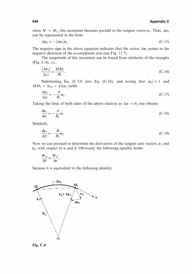
when M ! M1; this increment becomes parallel to the tangent vector e1. Thus, �e3can be represented in the form

�e3 ¼ � �e3 e1: ðC:15Þ

The negative sign in the above equation indicates that the vector �e3 points in thenegative direction of the -coordinate axis (see Fig. 11.7).

The magnitude of this increment can be found from similarity of the triangles(Fig. C.4), i.e.,

�e3 e3 ¼ MM1

R1

: ðC:16Þ

Substituting Eq. (C.15) into Eq. (C.16), and noting that e3 ¼ 1 and

MM1 ¼ �s ¼ A�, yields

�e3

�¼ � A

R1

e1: ðC:17Þ

Taking the limit of both sides of the above relation as �! 0, one obtains

de3d

¼ � A

R1

e1: ðC:18Þ

Similarly,

de3d

¼ � B

R2

e2: ðC:19Þ

Now we can proceed to determine the derivatives of the tangent unit vectors, e1 ande2, with respect to and . Obviously the following equality holds:

@r;@

¼ @r;@

;

because it is equivalent to the following identity:

646 Appendix C

Fig. C.4

@2r

@@¼ @2r

@@:

From the above, and taking into account the relations (11.10) and (11.12), we obtain

@

@Ae1ð Þ ¼ @

@Be2ð Þ: ðC:20aÞ

The derivatives of the unit tangent vectors can be expressed in terms of their com-ponents along the triad of the unit vectors e1; e2; and e3. Notice that the derivative ofany unit tangent vector is normal to the vector itself, so that there are no componentsin the direction of the vector being differentiated. Let us prove this statement.Consider the following scalar product of the two unit tangent vectors in the curvi-linear coordinate system:

ei � ej ¼ �ij�ij ¼ 1 if i ¼ j;�ij ¼ 0 if i 6¼ j;

where i; j ¼ 1; 2; and 3. Differentiating the scalar product of the two unit vectorswith respect to k (k ¼ 1 or 2) yields

ei � ej� �

;k¼ 0;

from which

ej � ei;k þ ei � ej;k ¼ 0:

Setting i ¼ j yields

2 ei � ei;k� � ¼ 0;

as was to be shown.First, determine the derivative @e1=@. As follows from the above, this deriva-

tive can be represented in terms of its components in the directions of e2 and e3 only.We have

@e1@

¼ qe2 þ te3; ðC:20bÞ

where unknown components q and t represent the projections of the vector @e1=@on the directions of e2 and e3, respectively. It is known from the vector algebra thatthe projection of any vector a on the direction of a vector b is equal to the scalarproduct of a � b. Therefore, the component q is given by

q ¼ e2 �@e1@

� �¼ @

@e2 � e1ð Þ � e1 �

@e2@

� �¼ �e1 �

@e2@

ðC:21Þ

@

@e2 � e1ð Þ ¼ 0 because e2 is normal to e1

� �:

It follows from Eq. (C.20a) that

@

@ðBe2Þ ¼ B

@e2@

þ e2@B

@¼ @

@ðAe1Þ: ðC:22Þ

Thus,

Verification of Theory of Surfaces 647

Appendix D

Derivation of the Strain–DisplacementRelations

D.1 VARIATION OF THE DISPLACEMENTS ACROSS THE SHELLTHICKNESS

Referring to Fig. 12.2, we can write the following vector equation:

Dz þ ze3 � ze 3 ¼ D; ðD:1Þ

where D and Dz are displacement vectors of pointsM and Mz, located on the middle

and on the equidistant surfaces of the shell, separated by a distance z, respectively; e 3is the unit normal vector of a deformed middle surface at point M1. From Eq. (D.1),it follows that

Dz ¼ Dþ e

z3 � e3ð Þz: ðD:2Þ

With the accuracy within the terms of the order of h=Rð Þ2 compared with unity, theunit normal vector e 3 can be determined by the following equality:

e 3 ¼ e

1 e

2; ðD:3aÞ

where e 1 and e

2 are the unit vectors tangent to the - and -coordinate lines on the

deformed middle surface. The equation of the deformed middle surface can berepresented in the following vector form:

r ð; Þ ¼ rð; Þ þD ¼ rð; Þ þ ue1 þ ve2 þ we3; ðD:3bÞ

where r ð; Þ is a position vector of the deformed middle surface of the shell. Notethat from here on, all functions and quantities associated with the deformed middlesurface will be denoted by an asterisk.

Using Eq. (11.24), we can write

e 1 ¼

r ;

A ; ðD:4Þ

where

A ¼ ffiffiffiffiffiffiffiffiffiffiffiffiffiffir ; � r ;

p: ðD:5Þ

651

Write out the vector r ; in the following expanded form:

r ; ¼

@r

@¼ @

@rþ ue1 þ ve2 þ we3ð Þ ¼ A"1 þ u

@e1@

þ v@e2@

þ w@"3@

þ @u

@e1 þ

@v

@e2 þ

@w

@e3:

ðD:6Þ

Substituting for the first derivative of the unit vectors from the relations (11.26) intothe above, yields the following:

r ; ¼ A 1þ 1

A

@u

@þ v

AB

@A

@� w

R1

� �e1 þ � u

B

@A

@þ @v

@

� �e2 þ

A

R1

uþ @w@

� �e3:

ðD:7ÞLet us determine the Lame parameter A of the deformed surface. It follows fromEqs (11.10) and (11.12) that A ð Þ2¼ r ; � r ;. Calculating the above scalar product,neglecting the products of displacements and their derivatives as small quantities ofthe second order, and retaining the terms depending linearly on the displacementsand their derivatives only, we obtain

A ð Þ2¼ A2 1þ 1

A

@u

@þ v

AB

@A

@� w

R1

� �2

; ðD:8Þ

from which

A ¼ Að1þ "1Þ; ðD:9Þwhere

"1 ¼1

A

@u

@þ v

AB

@A

@� w

R1

: ðD:10Þ

Using Eqs (D.8)–(D.10), one can represent the unit tangent vector e 1 as follows:

e 1 ¼

r ;

A ¼1

Að1þ "Þ A 1þ 1

A

@u

@þ v

AB

@A

@� w

R1

� ��e1

þ @v

@� u

B

@A

@

� �e2 þ

A

R1

uþ @w@

� �e3

�:

ðD:11Þ

Due to the small-displacement assumption, adopted in the linear theory of thinshells, all the strain components are negligible quantities in comparison withunity. Following this degree of accuracy, we can obtain from the above the followingfinal expression for e 1:

e 1 ffi e1 þ !1e2 þ #1e3: ðD:12aÞ

Similarly, we can obtain

e 2 ffi e2 þ !2e1 þ #2e3; ðD:12bÞ

where

652 Appendix D

!1 ¼1

A

@v

@� 1

AB

@A

@u; !2 ¼

1

B

@u

@� 1

AB

@B

@v;

#1 ¼u

R1

þ 1

A

@w

@; #2 ¼

v

R2

þ 1

B

@w

@:

ðD:13Þ

To clarify the geometric meaning of the parameters !1; !2; #1; and #2 we set up thecross-products of the vectors e1 and e

1 and the vectors e 2 and e2. Using Eqs (D.12)

and the properties of the cross-products of the unit vectors, we obtain the following:

e1 e 1 ¼ e3!1 � e2#1; e

2 e2 ¼ e3!2 � e1#2:

The right-hand sides of the above relations represent the sines of angles by which theunit tangent vectors e1 and e2 rotate because of a deformation of the middle surface.Due to the small-displacement assumption, these sines are small quantities of the firstorder and they may be identified with the angles of rotations themselves. Thus, therotation of the unit vector e1 consists of the rotation through the angle !1 about thedirection e3 and of the rotation through the angle #1 about the direction e2:Correspondingly, the rotation of the vector e2 comprises the rotation through theangle !2 about e3 and through the angle #2 about e1.

Introducing the relations (D.12) into Eqs (D.3a) and neglecting the terms ofsecond differential order, we obtain, after some mathematics, the following:

e 3 ffi e3 � #1e1 � #2e2: ðD:14Þ

Inserting the above expression into the relation (D.2) yields the following:

Dz ¼ Dþ e3 � #1e1 � #2e2 � e3ð Þz or

Dz ¼ D� #1e1 þ #2e2ð Þz:

ðD:15Þ

Projecting this vector on the directions of the unit vectors e1; e2; and e3, we obtainthe three scalar equations (12.1).

D.2 STRAIN COMPONENTS OF THE SHELL

Consider two neighboring points Mð; Þ and M1ðþ d; Þ lying on the line ¼const of the shell middle surface. The distance between these points is

� before deformation � ds1 ¼ Ad; ðD:16aÞ� after deformation � ds 1 ¼ A d ðD:16bÞ

The relative increase in length of a curvilinear linear element of the middle surface inthe direction of the -coordinate line is

ds 1 � ds1ds1

:

Substituting for ds 1 and ds1 from Eqs (D.16) into the above and taking into accountEqs (D.9) and (D.10), we obtain the expression for the linear strain in the direction,"1, in terms of the displacement components at a point of the middle surface in the direction. Similarly, the expression for "2 can be obtained. The above strain–displacement components are given by Eqs (12.3) and (12.4).

Derivation of Strain–Displacement Relations 653

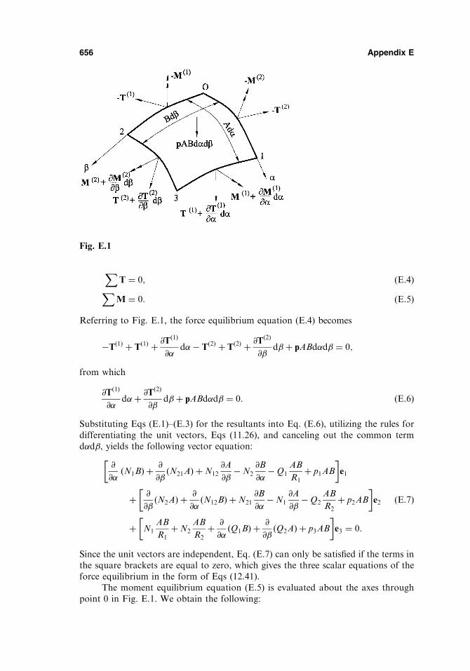
XT ¼ 0; ðE:4ÞXM ¼ 0: ðE:5Þ

Referring to Fig. E.1, the force equilibrium equation (E.4) becomes

�Tð1Þ þ T

ð1Þ þ @Tð1Þ

@d� T

ð2Þ þ Tð2Þ þ @T

ð2Þ

@dþ pABdd ¼ 0;

from which

@Tð1Þ

@dþ @T

ð2Þ

@dþ pABdd ¼ 0: ðE:6Þ

Substituting Eqs (E.1)–(E.3) for the resultants into Eq. (E.6), utilizing the rules fordifferentiating the unit vectors, Eqs (11.26), and canceling out the common termdd, yields the following vector equation:

@

@

�ðN1BÞ þ

@

@ðN21AÞ þN12

@A

@�N2

@B

@�Q1

AB

R1

þ p1AB

�e1

þ @

@ðN2AÞ þ

@

@ðN12BÞ þN21

@B

@�N1

@A

@�Q2

AB

R2

þ p2AB

� �e2

þ N1

AB

R1

þN2

AB

R2

þ @

@ðQ1BÞ þ

@

@ðQ2AÞ þ p3AB

� �e3 ¼ 0:

ðE:7Þ

Since the unit vectors are independent, Eq. (E.7) can only be satisfied if the terms inthe square brackets are equal to zero, which gives the three scalar equations of theforce equilibrium in the form of Eqs (12.41).

The moment equilibrium equation (E.5) is evaluated about the axes throughpoint 0 in Fig. E.1. We obtain the following:

656 Appendix E

Fig. E.1

Mð1Þ þ @M

ð1Þ

@d�M

ð1Þ þMð2Þ þ @M

ð2Þ

@d�M

ð2Þ þ Ad e1 Tð1Þ

� �

þ Bd e2 Tð2Þ

� �¼ 0;

from which

@Mð1Þ

@dþ @M

ð2Þ

@dþ Ad e1 T

ð1Þ� �

þ Bd e2 Tð2Þ

� �¼ 0: ðE:8Þ

The third and fourth terms in Eq. (E.8) represent the contribution of the resultantvectors TðiÞ ði ¼ 1; 2Þ to the moment equilibrium equation (E.5). It is easy to verifythat the in-plane shear forces N12 and N21 will contribute moments about the e3 axis,while the transverse shear forces Q1 and Q2 will contribute moments about the e1and e2 axes.

In setting up Eq. (E.8), only terms of the second differential order wereretained; terms of the third differential order were dropped out. Note that themoments due to the surface load p and due to the increments of the forces T

ð1Þ

and Tð2Þ also resulted in an appearance of the terms of the third differential order.Substituting for M

ð1Þ; Mð2Þ; Tð1Þ; and Tð2Þ from Eqs (E.1) and (E.2) into Eq.

(E.8), taking into account the relations (11.26) for the differentiation of the unitvectors, and canceling out the common factor dd, we obtain the following vectorequation:

M1

@A

@

�� @

@ðM12BÞ �M21

@B

@� @

@ðM2AÞ þQ2AB

�"1

þ @

@ðM1BÞ þM12

@A

@þ @

@ðM21AÞ �M2

@B

@�Q1AB

� �e2

þ �M12

AB

R1

þM21

AB

R2

þ ðN12 �N21ÞAB� �

e3 ¼ 0:

ðE:9Þ

This vector equation is equivalent to the three scalar equations (12.42).

Verification of Equilibrium Equations 657

Index

Airy stress function, 14, 220, 497, 500, 569

Angles of rotation in:

plates, 18, 209, 211

shells, 327, 653

Anisotropic plates (see Orthotropic plates)

Anisotropic shells (see Orthotropic shells)

Annular circular plates (see Circular plates)

Approximate and numerical methods (see

Numerical and approximate methods)

Approximate theories of shells (see specific

theories)

Assumptions of

classical plate theory, 7, 8

classical shell theory, 325

Asymmetrically loaded, membrane theory:

conical shells, 365–367

cylindrical shells, 361–365, 380–383,

400–402

shells of revolution, 352–356, 387–390

Asymmetrically loaded, moment theory:

circular cylindrical shells, 412–420

circular plates, 116–119

shells of revolution, 449–454

Axisymmetrically loaded, membrane theory:

conical shells, 367–368, 379, 380

circular cylindrical shells, 394–399, 402–404

shells of revolution, 356–361, 373–378

Axisymmetrically loaded, moment theory:


[Axisymmetrically loaded, moment theory]


conical shells, 475–478


toroidal shells, 478, 479

Barrel shells, 380, 418

Basic state of stress, 416, 507, 586

Beam functions, 620

Bending curvature of plates, 19

Bending moments (see Stress couples)

Bending stiffness (see Flexural stiffness)

Bending (moment) theory of:


shallow shells, 497–506


Bessel functions, 114, 253, 443

Betti-Maxwell reciprocal theorem, 119, 161,

198, 234

Bifurcation point, 242, 567, 569

Biharmonic equation, 25

Biharmonic operator, 25

Boundary collocation method, 152–156

Boundary conditions of:

plates, 26–35

shells, 341–344

Boundary element method, 156–166

Boussinesq’s solution for semi-infinite space,

80

659

Fourier series in (see also Navier’s and Levy’s

methods):

plate analysis, 47, 60, 116, 202, 214, 221,

246, 283, 503, 528, 577

shell analysis, 385, 416, 452, 503, 528, 577,

613, 617, 619, 621, 624

Fourier series expansion, 635–640

Free vibrations of:


conical shells, 618, 619

cylindrical shells, 610–618

rectangular plates, 276–284

shallow shells, 619–622

stiffened shells, 622–624

Frenet formula, 643

Frequency of forced vibrations for:

plates, 287

shells, 625

Fundamental natural frequency, 278, 280,

281, 286, 611, 618

Galerkin method, 166–171, 221, 222–230,

267, 528, 587, 598, 620

Gaussian curvature, 312

Geckeler’s approximation, 460–464

General-purpose equation, 440

Geometry of shell middle surface, 303–324,

643–645

Geometry of space curve, 641–643

Godunov’s method of discrete

orthogonalization, 444

Green’s function, 60, 434

Gridwork analogy, 26

Helmholtz equation, 210

Hooke’s law (see Constitutive equations)

Hyperbolic paraboloid, 47

membrane analysis of, 386, 387

Hyperboloid of revolution, 313, 314

Images method, 137

Inertia forces, 276, 609, 610

Initial curvature, bending of plates with,

88–90

Initial imperfections, impact on buckling of

thin shells, 567, 585–590, 602

Isothermal analogy, 195, 516

Isotropy material, 8

Intrinsic geometry of surface, 309

Jacobi matrix, 558

Kinematic boundary conditions, 35, 344

Kinematic (strain–displacement) relations of:

general linear shell theory, 331

linear elasticity, 10–12

linear plate bending theory, 18

nonlinear plate bending theory, 219

nonlinear shell theory, 523, 586

Kinetic energy of vibrating:

plate, 279

shell, 612, 615, 621

Kirchhoff, assumptions (see Assumptions of

the classical plate theory)

Kirchhoff-Love assumptions (see

Assumptions of the classical shell

theory)

Kirchhoff shear force (see Effective

(Kirchhoff) shear force)

Krylov’s functions, 438

Lagrange’s principle (see Principle of

minimum potential energy)

Lagrange’s theorem, 351

Lame parameters, 308, 652

Laplace elliptic operator, 496

Laplace operator, 22, 98, 226, 499

Large (finite) deflections (see Nonlinear

theories of plates and shells)

Levy’s equation, 14

Levy’s solution for rectangular plates (single

series solution), 60–71

Line of transition, 374

Lines of curvature (see Lines of principal

curvature)

Lines of distortion, 507

Lines of principal curvature (lines of

curvature), 306

Liquid storage facilities, membrane analysis

of:

cylindrical tanks:

asymmetric loading, 400–402

axisymmetric loading, 394–397

Intze tank, 397–400

spherical tanks:

asymmetric loading, 400–402

axisymmetric loading, 392–394

Live loads, 378, 379

Load-carrying capacity of plates in

compression, 267–270

Long cylinders, 425, 579, 582, 585

Material, table of properties, 630, 631

662 Index

Maxwell’s reciprocal theorem (see Betti-

Maxwell reciprocal theorem)

Membranes, 3, 207

Membrane state of stress, 299

Membrane theory:

applicability of, 351, 352

of conical shells, 365–368

constitutive equations, 350

of cylindrical shells

circular, 380–383, 401, 402

general, 361–365

equilibrium equations, 350

governing equations, 354, 355, 371

kinematic relations, 350

of shells of arbitrary shape, 368–371

shells of revolution, 352–361, 373–380,

387–394

Meridians, 313, 352

Meridional angle, 352, 450

Method of successive approximations, 553

Method of successive loadings, 555–557

Methods (see specific titles)

Middle surface (middle plane) of:

plate, 1,3

shell, 292

Minimum potential energy principle (see

Principle of minimum potential energy)

Mixed state of stress, 346

Moderate-length, intermediate-length

cylinders, 579, 581, 618

Modulus of elasticity, table of various

materials, 630, 631

Momentless state of stress (see Membrane

state of stress)

Moments, bending and twisting (see also

Stress couples)

in plates, 20, 21

in shells, 335

Moment state of stress, 300, 346

Multilayered

plates, 231–233

shells, 538–541

Natural anisotropy, 197

Natural boundary conditions, 35, 344

Natural frequencies of vibration, 276–286,

611, 617, 621

methods for determination of, 278–284,

618–621

Navier’s method (double series solution),

47–54, 196, 501, 503, 504, 597, 613,

617, 619

Newton method, 557–561

Neutral equilibrium, 242, 566

Nodal displacements, 177, 547

Nodal forces, 177

Non-developable surfaces, 316

Nonlinear (geometrically) theory of:

plates, 215–231

shells, 522–531

Normal curvature (see Curvature of

normal section)

Normal (direct) force, 84, 335

Normal section, 304

Normal to surface, 304

Numerical and approximate methods for

solution of (see also specific

methods):

linear plate and shell problems, 143–188,

543–553

nonlinear equations, 553–561

Orthogonal curvilinear coordinate system,

304

Orthogonality of functions, 166

Orthotropic plates:

basic relationships for, 197–199

buckling, 259–265

circular, 204–207

constitutive equations (see Constitutive

equations for orthotropic plates)

governing equations, 199, 206

naturally, 197–199

rectangular, 202–204

rigidities, 199–201

strain energy in, 199

structurally (stiffened), 261–265

Orthotropic shells:

buckling, 590–594


equations for orthotropic shells)

governing equations, 535, 537, 538

naturally, 531, 532

structurally (stiffened), 532–538

Osculating plane, 644

Paraboloid of revolution, 320,

Parallel circle, 316, 352, 374, 450

Particular solution in:

plate bending problems, 44, ,61, 62, 64, 66,

78, 99, 104, 118, 135, 158

shell problems, 423, 425, 438, 441, 455,

486, 488, 518

Periodicity conditions, 341

Index 663

[Shallow shells]

kinematic relations, 499, 523, 524

large (finite) deflections of, 523–531

orthotropic and stiffened, 536–538

specialization of geometry, 323, 324

thermal stress analysis, 521, 522

Shape factor, 578

Shear buckling, 258, 259

Shear forces in:

plates, 21, 24–26

shells, 335

Shear stiffness of:

plates, 209

sandwich shells, 541

stiffened shells, 532

Shear strains, 11, 12

in plates, 18

in shells, 327, 329–331

Shells (see also specific types of shells in

alphabetical order):

approximate theories of, 483–511

boundary conditions, 341–344

classification of, 294, 313–316


equations for classical linear shell

theory)

definitions and fundamentals of, 292–294

equilibrium equations, 655–657

governing differential equations (see

specific types of shells)

kinematics of, 326–333

load carrying mechanism of, 299, 300

membrane theory of, 349–372 (see also

specific types of shells)

moment theory (see specific types of shells)

multilayered (see Multilayered shells)

nonlinear theory (see Nonlinear theory of

shells)

orthotropic and stiffened (see Orthotropic

and Stiffened shells)

outline of linear theories of, 294–299

sandwich (see Sandwich, bending of shells)

statics of, 333–337

strain energy of, 340, 341

stress (see Stress in shells)

stress resultants and couples, 334–337

thermal stresses in, 515–522

Shells of revolution:

constitutive equations, 354, 454

equilibrium equations, 353, 451

governing equations, 354, 355, 456, 457

kinematic relations, 354, 451, 454

[Shells of revolution]

membrane theory (see Membrane theory

of shells of revolution)

moment theory, 449–479

approximate method for solution (see

Geckeler’s approximation)

Shell stability (see Stability theory)

Short cylinder, 437, 577, 579, 581

Simple edge effect, 507

Singly curved shells, 315

Skew plates, 139, 140

Small parameter method, 81–83, 554, 555

Snap-through buckling, 567

Snow loads (see Live loads)

Space curve, 641–643

Specific stress functions, 495 (see also Pucher

stress function)

Spherical shells (see also Domes):

buckling of, 600–602

membrane theory of, 373–379, 387–390,

392–394, 403, 404

moment theory of, 464–473

Stability theory:

energy method, 255–259

equilibrium method, 245–255

governing equations, 243, 570–572

Stable equilibrium, 242, 244, 566, 567, 572

Stationary condition, 40, 244, 572

Stiffened plates

bending of:

circular, 204–208

rectangular, 199–204

buckling of, 261–265

Stiffened shells:

bending of, 532–538

buckling of, 591–595, 605, 606

Stiffening rings (see Ring reinforcing, of

cylindrical shells)

Stiffness matrix in:

plates, 181, 182

shells, 548, 550, 553

Stiff plates, 3

Strain-displacement relations (see Kinematic

relations)

Strain energy of:

plates, 35–38,

shells, 341

strip-beam, 612

Strain matrix,179

Stream function, 210:

Stress resultants and couples (see Plates and

Shells, stress resultants and couples)

Index 665

to - · pdf file8.2 general postulations of the theory of stability of plates 241 8.3 the...

Documents