TN0501

ADVANCED DIGITAL COMMUNICATIONS

M-TECH TELECOMMUNICATION NETWORKS

LAB COMPONENT MANUAL

DEPARTMENT OF TELECOMMUNICATION ENGINEERING SRM UNIVERSITY

S.R.M. NAGAR, KATTANKULATHUR – 603 203

FOR PRIVATE CIRCULATION ONLY ALL RIGHTS RESERVED

1 

 

TN0501

ADVANCED DIGITAL COMMUNICATIONS

M-TECH TELECOMMUNICATION NETWORKS

LAB COMPONENT MANUAL

DEPARTMENT OF TELECOMMUNICATION ENGINEERING SRM UNIVERSITY

S.R.M. NAGAR, KATTANKULATHUR – 603 203

FOR PRIVATE CIRCULATION ONLY ALL RIGHTS RESERVED

2  

3  

DEPARTMENT OF TELECOMMUNICATION ENGINEERING

TN0501 ADVANCED DIGITAL COMMUNICATIONS

(2012-2013) Revision no: 01 PREPARED BY,

Mrs . DEEPA . T

HOD / TCE

4  

TN0501 – Advanced Digital Communication List of Experiments

Date of Exam:

Exp.No. EXPERIMENTS

1. Amplitude Shift Keying

2. Frequency Shift Keying

3. Phase Shift Keying signal

4. Quadrature Phase Shift Keying (QPSK)

5. QPSK with Rayleigh fading & AWGN

6. M-ary QAM with AWGN fading

7. BER For BPSK Modulation With ZFE Equalizer In 3 Tap ISI Channel

8. BER for BPSK modulation with Minimum Mean Square Error (MMSE) equalization in 3 tap ISI channel.

9. Comparative analysis of BER for BPSK modulation in 3 tap ISI channel with ZFE and MMSE Equalization

10. Lease Mean Square (LMS) Algorithm

EXPERIMENT 1 Amplitude Shift Keying

AIM:- To plot the wave form for Binary Amplitude Shift Keying (BASK) signal using MATLAB for a stream of bits.

THEORY:-

Amplitude Shift Keying (ASK) is the digital modulation technique. In amplitude shift keying, the amplitude of the carrier signal is varied to create signal elements. Both frequency and phase remain constant while the amplitude changes. In ASK, the amplitude of the carrier assumes one of the two amplitudes dependent on the logic states of the input bit stream. This modulated signal can be expressed as:

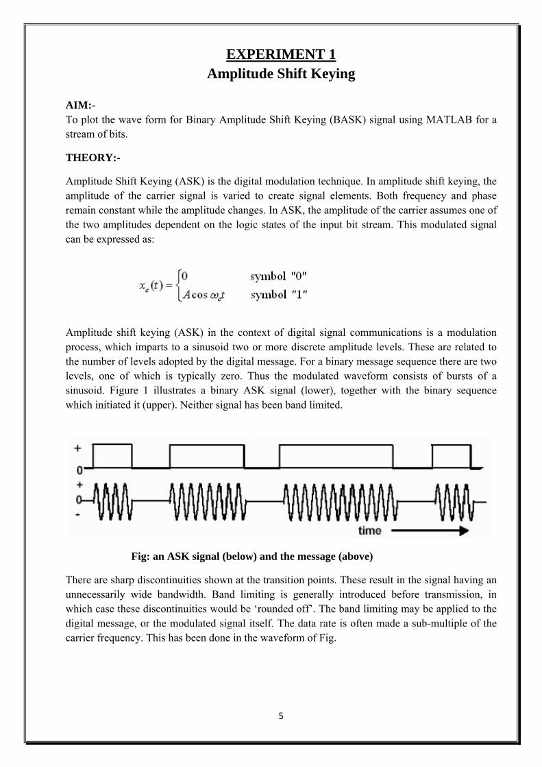
Amplitude shift keying (ASK) in the context of digital signal communications is a modulation process, which imparts to a sinusoid two or more discrete amplitude levels. These are related to the number of levels adopted by the digital message. For a binary message sequence there are two levels, one of which is typically zero. Thus the modulated waveform consists of bursts of a sinusoid. Figure 1 illustrates a binary ASK signal (lower), together with the binary sequence which initiated it (upper). Neither signal has been band limited.

Fig: an ASK signal (below) and the message (above)

There are sharp discontinuities shown at the transition points. These result in the signal having an unnecessarily wide bandwidth. Band limiting is generally introduced before transmission, in which case these discontinuities would be ‘rounded off’. The band limiting may be applied to the digital message, or the modulated signal itself. The data rate is often made a sub-multiple of the carrier frequency. This has been done in the waveform of Fig.

5  

6  

MATLAB PROGRAM:- clear; clc; b = input('Enter the Bit stream \n '); %b = [0 1 0 1 1 1 0]; n = length(b); t = 0:.01:n; x = 1:1:(n+1)*100; for i = 1:n for j = i:.1:i+1 bw(x(i*100:(i+1)*100)) = b(i); end end bw = bw(100:end); sint = sin(2*pi*t); st = bw.*sint; subplot(3,1,1) plot(t,bw) grid on ; axis([0 n -2 +2]) subplot(3,1,2) plot(t,sint) grid on ; axis([0 n -2 +2]) subplot(3,1,3) plot(t,st) grid on ; axis([0 n -2 +2])

OBSERVATION:- Output waveform for the bit stream [0 1 0 0 1 1 1 0]

Output waveform for the bit stream [1 0 1 1 0 0 0 1]

7 

 

EXPERIMENT 2 Frequency Shift Keying

AIM:- To plot the wave form for Binary Frequency Shift Keying (BFSK) signal using MATLAB for a stream of bits.

THEORY:-

In frequency-shift keying, the signals transmitted for marks (binary ones) and spaces (binary zeros) are respectively.

This is called a discontinuous phase FSK system, because the phase of the signal is discontinuous at the switching times. A signal of this form can be generated by the following system.

If the bit intervals and the phases of the signals can be determined (usually by the use of a phase-lock loop), then the signal can be decoded by two separate matched filters:

The first filter is matched to the signal S1(t)and the second to S2(t) Under the assumption that the signals are mutually orthogonal, the output of one of the matched filters will be E and the other zero (where E is the energy of the signal). Decoding of the bandpass signal can therefore be achieved by subtracting the outputs of the two filters, and comparing the result to a threshold. If the signal S1(t) is present then the resulting output will be +E, and if S2(t) is present it will be –E. Since the noise variance at each filter output is En/2, the noise in the difference signal will be doubled, namely �2

=En. Since the overall output variation is 2E, the probability of error is:

8  

9  

MATLAB PROGRAM:-

clear; clc; b = input('Enter the Bit stream \n '); %b = [0 1 0 1 1 1 0]; n = length(b); t = 0:.01:n; x = 1:1:(n+1)*100; for i = 1:n if (b(i) == 0) b_p(i) = -1; else b_p(i) = 1; end for j = i:.1:i+1 bw(x(i*100:(i+1)*100)) = b_p(i); end end bw = bw(100:end); wo = 2*(2*pi*t); W = 1*(2*pi*t); sinHt = sin(wo+W); sinLt = sin(wo-W); st = sin(wo+(bw).*W); subplot(4,1,1) plot(t,bw) grid on ; axis([0 n -2 +2]) subplot(4,1,2) plot(t,sinHt) grid on ; axis([0 n -2 +2]) subplot(4,1,3) plot(t,sinLt) grid on ; axis([0 n -2 +2]) subplot(4,1,4) plot(t,st) grid on ; axis([0 n -2 +2]) Fs=1; figure %pburg(st,10) periodogram(st)

OBSERVATION:-

Output waveform for the bit stream [0 1 0 0 1 1 1 0]

10 

 

Output waveform for the bit stream [1 0 1 1 0 0 0 1]

11  

EXPERIMENT 3 Phase Shift Keying signal

AIM:- To plot the wave form for Binary Phase Shift Keying signal (BPSK) using MATLAB for a stream

of bits.

THEORY:-

In carrier-phase modulation, the information that is transmitted over a communication channel is

impressed on the phase of the carrier. Science the range of the carrier phase is 0 ≤ θ ≤ 2Π,the

carrier phases used to transmit digital information via digital-phase modulation are θm=2Πm/M,

for m=0,1,2…..,M-1.Thus for binary phase modulation(M=2),the two carrier phase are θ0 =0 and

θ1 = Π radian. For M-array phase modulation=2k, where k is the number of information bits per

transmitted symbol.

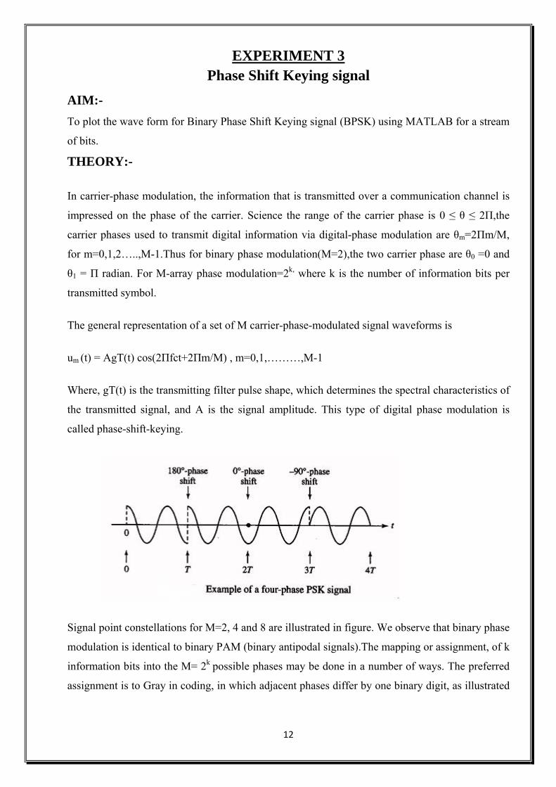
The general representation of a set of M carrier-phase-modulated signal waveforms is

um (t) = AgT(t) cos(2Πfct+2Πm/M) , m=0,1,………,M-1

Where, gT(t) is the transmitting filter pulse shape, which determines the spectral characteristics of

the transmitted signal, and A is the signal amplitude. This type of digital phase modulation is

called phase-shift-keying.

Signal point constellations for M=2, 4 and 8 are illustrated in figure. We observe that binary phase

modulation is identical to binary PAM (binary antipodal signals).The mapping or assignment, of k

information bits into the M= 2k possible phases may be done in a number of ways. The preferred

assignment is to Gray in coding, in which adjacent phases differ by one binary digit, as illustrated

12  

below in the figure. Consequently, only a single bit error occurs in the k-bit sequence with Gray

encoding when noise causes the incorrect selection of an adjacent phase to the transmitted phase

In figure shows that, block diagram of M=4 PSK system. The uniform random number generator

fed to the 4-PSK mapper and also fed to the compare. The 4-PSK mapper split up into two phases.

On the other hand, Gaussian RNG adds to the modulator. The two phases are fed to the detector.

The output goes to the compare. The Uniform random number generator and detector also fed to

the detector and finally fed to the bit-error counter and symbol-error counter.

MATLAB PROGRAM:- clear;

clc;

b = input('Enter the Bit stream \n '); %b = [0 1 0 1 1 1 0];

n = length(b);

t = 0:.01:n;

x = 1:1:(n+1)*100;

for i = 1:n

if (b(i) == 0)

b_p(i) = -1;

else

b_p(i) = 1;

end

for j = i:.1:i+1

bw(x(i*100:(i+1)*100)) = b_p(i);

end

end

13  

14  

bw = bw(100:end);

sint = sin(2*pi*t);

st = bw.*sint;

subplot(3,1,1)

plot(t,bw)

grid on ; axis([0 n -2 +2])

subplot(3,1,2)

plot(t,sint)

grid on ; axis([0 n -2 +2])

subplot(3,1,3)

plot(t,st)

grid on ; axis([0 n -2 +2])

OBSERVATION:- Output waveform for the bit stream [0 1 0 0 1 1 1 0]

Output waveform for the bit stream [1 0 1 1 0 0 0 1]

15  

EXPERIMENT 4

Quadrature Phase Shift Keying AIM:- To plot the wave form for Quadrature Phase Shift Keying (QPSK) signal using MATLAB for a

stream of bits.

THEORY:- Quadrature Phase Shift Keying (QPSK) is the digital modulation technique.Quadrature Phase

Shift Keying (QPSK) is a form of Phase Shift Keying in which two bits are modulated at once,

selecting one of four possible carrier phase shifts (0, Π/2, Π, and 3Π/2). QPSK perform by

changing the phase of the In-phase (I) carrier from 0° to 180° and the Quadrature-phase (Q)

carrier between 90° and 270°. This is used to indicate the four states of a 2-bit binary code. Each

state of these carriers is referred to as a Symbol.

QPSK perform by changing the phase of the In-phase (I) carrier from 0° to 180° and the

Quadrature-phase (Q) carrier between 90° and 270°. This is used to indicate the four states of a 2-

bit binary code. Each state of these carriers is referred to as a Symbol. Quadrature Phase-shift

Keying (QPSK) is a widely used method of transferring digital data by changing or modulating

the phase of a carrier signal. In QPSK digital data is represented by 4 points around a circle which

correspond to 4 phases of the carrier signal. These points are called symbols. Fig. shows this

mapping.

16  

17  

MATLAB PROGRAM:- clear;

clc;

b = input('Enter the Bit stream \n '); %b = [0 1 0 1 1 1 0];

n = length(b);

t = 0:.01:n;

x = 1:1:(n+2)*100;

for i = 1:n

if (b(i) == 0)

b_p(i) = -1;

else

b_p(i) = 1;

end

for j = i:.1:i+1

bw(x(i*100:(i+1)*100)) = b_p(i);

if (mod(i,2) == 0)

bow(x(i*100:(i+1)*100)) = b_p(i);

bow(x((i+1)*100:(i+2)*100)) = b_p(i);

else

bew(x(i*100:(i+1)*100)) = b_p(i);

bew(x((i+1)*100:(i+2)*100)) = b_p(i);

end

if (mod(n,2)~= 0)

bow(x(n*100:(n+1)*100)) = -1;

bow(x((n+1)*100:(n+2)*100)) = -1;

end

end

end %be = b_p(1:2:end);

%bo = b_p(2:2:end);

bw = bw(100:end);

bew = bew(100:(n+1)*100);

bow = bow(200:(n+2)*100);

cost = cos(2*pi*t);

sint = sin(2*pi*t);

st = bew.*cost+bow.*sint;

18  

subplot(4,1,1)

plot(t,bw)

grid on ; axis([0 n -2 +2])

subplot(4,1,2)

plot(t,bow)

grid on ; axis([0 n -2 +2])

subplot(4,1,3)

plot(t,bew)

grid on ; axis([0 n -2 +2])

subplot(4,1,4)

plot(t,st)

grid on ; axis([0 n -2 +2])

OBSERVATION:- Output waveform for the bit stream [0 1 0 0 1 1 1 0]

Output waveform for the bit stream [1 0 1 1 0 0 0 1]

19  

EXPERIMENT 5

QPSK with Rayleigh fading & AWGN AIM:- To plot the wave forms for QPSK signal subjected to rayleigh AWGN using MATLAB.

THEORY:- Quadrature Phase Shift Keying (QPSK) is the digital modulation technique.Quadrature Phase

Shift Keying (QPSK) is a form of Phase Shift Keying in which two bits are modulated at once,

selecting one of four possible carrier phase shifts (0, Π/2, Π, and 3Π/2). QPSK perform by

changing the phase of the In-phase (I) carrier from 0° to 180° and the Quadrature-phase (Q)

carrier between 90° and 270°. This is used to indicate the four states of a 2-bit binary code. Each

state of these carriers is referred to as a Symbol.

Rayleigh fading is a statistical model for the effect of a propagation environment on

a radio signal, such as that used by wireless devices.Rayleigh fading models assume that the

magnitude of a signal that has passed through such a transmission medium (also called

a communications channel) will vary randomly, or fade,according to a Rayleigh distribution —

the radial component of the sum of two uncorrelated Gaussian random variables.

Additive white Gaussian noise (AWGN) is a channel model in which the only impairment to

communication is a linear addition of wideband or white noise with a constant spectral

density (expressed as watts per hertz of bandwidth) and a Gaussian distribution of amplitude.

20  

21  

MATLAB PROGRAM:-

clear all; close all; format long; bit_count = 10000; Eb_No = -3: 1: 30; SNR = Eb_No + 10*log10(2); for aa = 1: 1: length(SNR) T_Errors = 0; T_bits = 0; while T_Errors < 100 uncoded_bits = round(rand(1,bit_count)); B1 = uncoded_bits(1:2:end); B2 = uncoded_bits(2:2:end); qpsk_sig = ((B1==0).*(B2==0)*(exp(i*pi/4))+(B1==0).*(B2==1)... *(exp(3*i*pi/4))+(B1==1).*(B2==1)*(exp(5*i*pi/4))... +(B1==1).*(B2==0)*(exp(7*i*pi/4))); ray = sqrt(0.5*((randn(1,length(qpsk_sig))).^2+(randn(1,length(qpsk_sig))).^2)); rx = qpsk_sig.*ray; N0 = 1/10^(SNR(aa)/10); rx = rx + sqrt(N0/2)*(randn(1,length(qpsk_sig))+i*randn(1,length(qpsk_sig))); rx = rx./ray; B4 = (real(rx)<0); B3 = (imag(rx)<0); uncoded_bits_rx = zeros(1,2*length(rx)); uncoded_bits_rx(1:2:end) = B3; uncoded_bits_rx(2:2:end) = B4; diff = uncoded_bits - uncoded_bits_rx; T_Errors = T_Errors + sum(abs(diff)); T_bits = T_bits + length(uncoded_bits); end figure; clf; plot(real(rx),imag(rx),'o'); % Scatter Plot title(['constellation of received symbols for SNR = ', num2str(SNR(aa))]); xlabel('Inphase Component'); ylabel('Quadrature Component'); BER(aa) = T_Errors / T_bits;

22  

disp(sprintf('bit error probability = %f',BER(aa))); end figure(1); semilogy(SNR,BER,'or'); hold on; xlabel('SNR (dB)'); ylabel('BER'); title('SNR Vs BER plot for QPSK Modualtion in Rayleigh Channel'); figure(1); EbN0Lin = 10.^(Eb_No/10); theoryBerRay = 0.5.*(1-sqrt(EbN0Lin./(EbN0Lin+1))); semilogy(SNR,theoryBerRay); grid on; figure(1); theoryBerAWGN = 0.5*erfc(sqrt(10.^(Eb_No/10))); semilogy(SNR,theoryBerAWGN,'g-+'); grid on; legend('Simulated', 'Theoretical Raylegh', 'Theroretical AWGN'); axis([SNR(1,1) SNR(end-3) 0.00001 1]);

23  

OBSERVATION:- Output data:- bit error probability = 0.211700 bit error probability = 0.197600 bit error probability = 0.169700 bit error probability = 0.151700 bit error probability = 0.119500 bit error probability = 0.107600 bit error probability = 0.091600 bit error probability = 0.077700 bit error probability = 0.063000 bit error probability = 0.055400 bit error probability = 0.044400 bit error probability = 0.036600 bit error probability = 0.030600 bit error probability = 0.023700 bit error probability = 0.020300 bit error probability = 0.017300 bit error probability = 0.011000 bit error probability = 0.009650 bit error probability = 0.007350 bit error probability = 0.006700 bit error probability = 0.005167 bit error probability = 0.004233 bit error probability = 0.003767 bit error probability = 0.002400 bit error probability = 0.001983 bit error probability = 0.001529 bit error probability = 0.001122 bit error probability = 0.001055 bit error probability = 0.000777 bit error probability = 0.000644 bit error probability = 0.000452 bit error probability = 0.000446 bit error probability = 0.000306 bit error probability = 0.000289

OBSERVATION:-

24  

25  

EXPERIMENT 6

8-QAM AIM:- To plot the wave form for 8 quadrature amplitude modulated signal (QAM) using MATLAB for a

stream of bits.

THEORY:- Quadrature amplitude modulation (QAM) is both an analog and a digital modulation scheme. It

conveys two analog message signals, or two digital bit streams, by changing (modulating) the

amplitudes of two carrier waves, using the amplitude-shift keying (ASK) digital modulation

scheme or amplitude modulation (AM) analog modulation scheme. The two carrier waves,

usually sinusoids, are out of phase with each other by 90° and are thus called quadrature carriers

or quadrature components — hence the name of the scheme. The modulated waves are summed,

and the resulting waveform is a combination of both phase-shift keying (PSK) and amplitude-shift

keying (ASK), or (in the analog case) of phase modulation (PM) and amplitude modulation. In the

digital QAM case, a finite number of at least two phases and at least two amplitudes are used.

PSK modulators are often designed using the QAM principle, but are not considered as QAM

since the amplitude of the modulated carrier signal is constant. QAM is used extensively as a

modulation scheme for digital telecommunication systems. Spectral efficiencies of 6 bits/s/Hz can

be achieved with QAM.

The 4-QAM and 8-QAM constellations

Time domain for an 8-QAM signal

26 

 

MATLAB PROGRAM:-

clc

close all

m=8

k=log2(m);

n=9e3;

nsamp=1;

x=randint(n,1);

stem(x(1:20),'filled');

title('bit sequence');

xlabel('bit index');

ylabel('bit amplitude');

xsym=bi2de(reshape(x,k,length(x)/k).','left-msb');

figure;

stem(xsym(1:10));

title('symbol plot');

xlabel('symbol index');

ylabel('symbol amplitude');

y=modulate(modem.qammod(m),xsym);

ytx=y;

ebno=10

snr=ebno+10*log(k)-10*log10(nsamp);

yn=awgn(ytx,snr); 27 

 

yrx=yn;

scatterplot(y);

scatterplot(yrx,30);

OBSERVATION:-

28  

29  

30 

 

31  

EXPERIMENT 7

BER performance for 16-QAM Modualtion in Rayleigh Channel

MATLAB PROGRAM:- % BER performance for 16-QAM Modualtion in Rayleigh fading Channel clear all; close all; % Frame Length 'Should be multiple of four or else padding is needed' bit_count = 1*1000; % Range of SNR over which to simulate Eb_No = 0: 1: 10; % Convert Eb/No values to channel SNR SNR = Eb_No + 10*log10(4); % Start the main calculation loop for aa = 1: 1: length(SNR) % Initiate variables T_Errors = 0; T_bits = 0; % Keep going until you get 100 errors while T_Errors < 100 % Generate some random bits uncoded_bits = round(rand(1,bit_count)); % Split the stream into 4 substreams B = reshape(uncoded_bits,4,length(uncoded_bits)/4); B1 = B(1,:); B2 = B(2,:); B3 = B(3,:); B4 = B(4,:); % 16-QAM modulator % normalizing factor a = sqrt(1/10); % bit mapping tx = a*(-2*(B3-0.5).*(3-2*B4)-j*2*(B1-0.5).*(3-2*B2)); % Variance = 0.5 - Tracks theoritical PDF closely ray =sqrt((1/2)*((randn(1,length(tx))).^2+(randn(1,length(tx))).^2)); % Include The Fading rx = tx.*ray; % Noise variance N0 = 1/10^(SNR(aa)/10);

32  

% Send over Gaussian Link to the receiver rx = rx + sqrt(N0/2)*(randn(1,length(tx))+1i*randn(1,length(tx))); % Equaliser rx = rx./ray; % 16-QAM demodulator at the Receiver a = 1/sqrt(10); B5 = imag(rx)<0; B6 = (imag(rx)<2*a) & (imag(rx)>-2*a); B7 = real(rx)<0; B8 = (real(rx)<2*a) & (real(rx)>-2*a); % Merge into single stream again temp = [B5;B6;B7;B8]; B_hat = reshape(temp,1,4*length(temp)); % Calculate Bit Errors diff = uncoded_bits - B_hat ; T_Errors = T_Errors + sum(abs(diff)); T_bits = T_bits + length(uncoded_bits); end % Calculate Bit Error Rate BER(aa) = T_Errors / T_bits; disp(sprintf('bit error probability = %f',BER(aa))); end % Finally plot the BER Vs. SNR(dB) Curve on logarithmic scale % BER through Simulation figure(1); semilogy(Eb_No,BER,'xr-','Linewidth',2); hold on; xlabel('E_b / N_o (dB)'); ylabel('BER'); title('E_b / N_o Vs BER plot for 16-QAM Modualtion in Rayleigh Channel'); % Theoretical BER figure(1); theoryBerAWGN = 0.5.*erfc(sqrt((10.^(Eb_No/10)))); semilogy(Eb_No,theoryBerAWGN,'g-+','Linewidth',2); grid on; legend('Rayleigh', 'AWGN'); axis([Eb_No(1,1) Eb_No(end) 0.00001 1]);

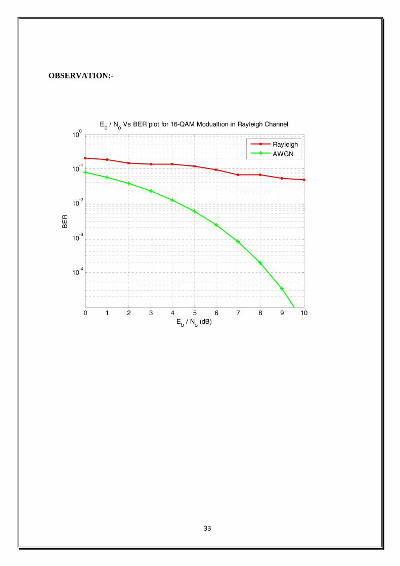
OBSERVATION:-

33  

0 1 2 3 4 5 6 7 8 9 10

10

-4

10

-3

10

-2

10

-1

10

0

Eb / N

o (dB)

BE

R

Eb / N

o Vs BER plot for 16-QAM Modualtion in Rayleigh Channel

Rayleigh

AWGN

34  

EXPERIMENT 8

BER for BPSK modulation with ZFE Equalizer in 3 tap ISI channel.

MATLAB PROGRAM:- % Script for computing the BER for BPSK modulation with ZFE Equalizer in 3 tap ISI channel. clc; clear N = 10^6; % number of bits or symbols Eb_N0_dB = [0:15]; % multiple Eb/N0 values K = 3; for ii = 1:length(Eb_N0_dB) % Transmitter ip = rand(1,N)>0.5; % generating 0,1 with equal probability s = 2*ip-1; % BPSK modulation 0 -> -1; 1 -> 0 % Channel model, multipath channel nTap = 3; ht = [0.2 0.9 0.3]; L = length(ht); chanOut = conv(s,ht); n = 1/sqrt(2)*[randn(1,N+length(ht)-1) + j*randn(1,N+length(ht)-1)]; % White gaussian noise, 0dB variance % Noise addition y = chanOut + 10^(-Eb_N0_dB(ii)/20)*n; % additive white gaussian noise % zero forcing equalization hM = toeplitz([ht([2:end]) zeros(1,2*K+1-L+1)], [ ht([2:-1:1]) zeros(1,2*K+1-L+1) ]) d = zeros(1,2*K+1); d(K+1) = 1; c_zf = [inv(hM)*d.'].'; yFilt_zf = conv(y,c_zf); yFilt_zf = yFilt_zf(K+2:end); yFilt_zf = conv(yFilt_zf,ones(1,1)); % convolutio n ySamp_zf = yFilt_zf(1:1:N); % sampling at time T % receiver - hard decision decoding ipHat_zf = real(ySamp_zf)>0; % counting the errors nErr_zf(1,ii) = size(find([ip- ipHat_zf]),2); end simBer_zf = nErr_zf/N; % simulated ber

% plot close all figure semilogy(Eb_N0_dB,simBer_zf(1,:),'bs-','Linewidth',2); hold on axis([0 14 10^-5 0.5]) grid on legend('BPSK System with ZFE EQUALIZER'); xlabel('Eb/No, dB'); ylabel('Bit Error Rate'); title('Bit error probability curve for BPSK in ISI with ZFE equalizer'); OBSERVATION:-

35  

0 2 4 6 8 10 12 14

10

-5

10

-4

10

-3

10

-2

10

-1

Eb/No, dB

Bit E

rror R

ate

Bit error probability curve for BPSK in ISI with ZFE equalizer

BPSK System with ZFE EQUALIZER

36  

EXPERIMENT 9

BER for BPSK modulation with Minimum Mean Square Error (MMSE) equalization in 3 tap ISI channel.

MATLAB PROGRAM:- % Script for computing the BER for BPSK modulation with Minimum Mean Square Error (MMSE) equalization with 7 tap in 3 tap ISI channel. % clear N = 10^6; % number of bits or symbols Eb_N0_dB = [0:15]; % multiple Eb/N0 values K = 3; for ii = 1:length(Eb_N0_dB) % Transmitter ip = rand(1,N)>0.5; % generating 0,1 with equal probability s = 2*ip-1; % BPSK modulation 0 -> -1; 1 -> 0 % Channel model, multipath channel nTap = 3; ht = [0.2 0.9 0.3]; L = length(ht); chanOut = conv(s,ht); n = 1/sqrt(2)*[randn(1,N+length(ht)-1) + j*randn(1,N+length(ht)-1)]; % white gaussian noise, 0dB variance % Noise addition y = chanOut + 10^(-Eb_N0_dB(ii)/20)*n; % additive white gaussian noise % mmse equalization hAutoCorr = conv(ht,fliplr(ht)) hM = toeplitz([hAutoCorr([3:end]) zeros(1,2*K+1-L)], [ hAutoCorr([3:end]) zeros(1,2*K+1-L) ]) hM = hM + 1/2*10^(-Eb_N0_dB(ii)/10)*eye(2*K+1); d = zeros(1,2*K+1); d([-1:1]+K+1) = fliplr(ht); c_mmse = [inv(hM)*d.'].'; yFilt_mmse = conv(y,c_mmse); yFilt_mmse = yFilt_mmse(K+2:end); yFilt_mmse = conv(yFilt_mmse,ones(1,1)); % convolution ySamp_mmse = yFilt_mmse(1:1:N); % sampling at time T % receiver - hard decision decoding ipHat_mmse = real(ySamp_mmse)>0; % counting the errors

nErr_mmse(1,ii) = size(find([ip- ipHat_mmse]),2); end simBer_mmse = nErr_mmse/N; % simulated ber theoryBer = 0.5*erfc(sqrt(10.^(Eb_N0_dB/10))); % theoretical ber % plot close all figure semilogy(Eb_N0_dB,simBer_mmse(1,:),'gd-','Linewidth',2); axis([0 14 10^-5 0.5]) grid on legend( 'BPSK system with MMSE EQUALIZER'); xlabel('Eb/No, dB'); ylabel('Bit Error Rate'); title('Bit error probability curve for BPSK in ISI with MMSE equalizer'); OBSERVATION:-

37  

0 2 4 6 8 10 12 14

10

-5

10

-4

10

-3

10

-2

10

-1

Eb/No, dB

Bit E

rror R

ate

Bit error probability curve for BPSK in ISI with MMSE equalizer

BPSK system with MMSE EQUALIZER

38  

EXPERIMENT 10

Comparative analysis of BER for BPSK modulation in 3 tap ISI channel with ZFE and MMSE Equalization

MATLAB PROGRAM:- % Script for computing the BER for BPSK modulation in 3 tap ISI channel. Minimum Mean Square Error (MMSE) equalization with 7 tap % and the BER computed (and is compared with Zero Forcing equalization) clear N = 10^6; % number of bits or symbols Eb_N0_dB = [0:15]; % multiple Eb/N0 values K = 3; for ii = 1:length(Eb_N0_dB) % Transmitter ip = rand(1,N)>0.5; % generating 0,1 with equal probability s = 2*ip-1; % BPSK modulation 0 -> -1; 1 -> 0 % Channel model, multipath channel nTap = 3; ht = [0.2 0.9 0.3]; L = length(ht); chanOut = conv(s,ht); n = 1/sqrt(2)*[randn(1,N+length(ht)-1) + j*randn(1,N+length(ht)-1)]; % white gaussian noise, 0dB variance % Noise addition y = chanOut + 10^(-Eb_N0_dB(ii)/20)*n; % additive white gaussian noise % zero forcing equalization hM = toeplitz([ht([2:end]) zeros(1,2*K+1-L+1)], [ ht([2:-1:1]) zeros(1,2*K+1-L+1) ]); d = zeros(1,2*K+1); d(K+1) = 1; c_zf = [inv(hM)*d.'].'; yFilt_zf = conv(y,c_zf); yFilt_zf = yFilt_zf(K+2:end); yFilt_zf = conv(yFilt_zf,ones(1,1)); % convolution ySamp_zf = yFilt_zf(1:1:N); % sampling at time T % mmse equalization hAutoCorr = conv(ht,fliplr(ht)) hM = toeplitz([hAutoCorr([3:end]) zeros(1,2*K+1-L)], [ hAutoCorr([3:end]) zeros(1,2*K+1-L) ]) hM = hM + 1/2*10^(-Eb_N0_dB(ii)/10)*eye(2*K+1); d = zeros(1,2*K+1); d([-1:1]+K+1) = fliplr(ht); c_mmse = [inv(hM)*d.'].';

39  

yFilt_mmse = conv(y,c_mmse); yFilt_mmse = yFilt_mmse(K+2:end); yFilt_mmse = conv(yFilt_mmse,ones(1,1)); % convolution ySamp_mmse = yFilt_mmse(1:1:N); % sampling at time T % receiver - hard decision decoding ipHat_zf = real(ySamp_zf)>0; ipHat_mmse = real(ySamp_mmse)>0; % counting the errors nErr_zf(1,ii) = size(find([ip- ipHat_zf]),2); nErr_mmse(1,ii) = size(find([ip- ipHat_mmse]),2); end simBer_zf = nErr_zf/N; % simulated ber simBer_mmse = nErr_mmse/N; % simulated ber theoryBer = 0.5*erfc(sqrt(10.^(Eb_N0_dB/10))); % theoretical ber % plot close all figure semilogy(Eb_N0_dB,simBer_zf(1,:),'bs-','Linewidth',2); hold on semilogy(Eb_N0_dB,simBer_mmse(1,:),'gd-','Linewidth',2); axis([0 14 10^-5 0.5]) grid on legend('BPSK system with ZFE EQUALIZER','BPSK system with MMSE EQUALIZER'); xlabel('Eb/No, dB'); ylabel('Bit Error Rate'); title('Bit error probability curve for BPSK in ISI with ZFE and MMSE equalizer');

OBSERVATION:-

40  

0 2 4 6 8 10 12 14

10

-5

10

-4

10

-3

10

-2

10

-1

Eb/No, dB

Bit E

rror R

ate

Bit error probability curve for BPSK in ISI with ZFE and MMSE equalizer

BPSK system with ZFE EQUALIZER

BPSK system with MMSE EQUALIZER

41  

EXPERIMENT 11

Lease Mean Square (LMS) Algorithm

MATLAB PROGRAM:- clc close all clear all N=1000; t=[0:N-1]; w0=0.001; phi=0.1; d=sin(2*pi*[1:N]*w0+phi); % desired signal x=d+randn(1,N)*0.5;% channel output w=zeros(1,N); mu=0.02; for i=1:N e(i) = d(i) - w(i)' * x(i); %error=desired signal-equalized signal w(i+1) = w(i) + mu * e(i) * x(i); % tap weight updation using LMS end for i=1:N yd(i) = sum(w(i+1)' * x(i)); % Adaptive Desired output end subplot(221),plot(t,d),ylabel('Desired Signal'), subplot(222),plot(t,x),ylabel('Input Signal+Noise'), subplot(223),plot(t,e),ylabel('Error'), subplot(224),plot(t,yd),ylabel('Adaptive Desired output');

OBSERVATION:-

 

42  

0 500 1000

-1

-0.5

0

0.5

1

Desired S

ignal

0 500 1000

-4

-2

0

2

4

Input S

ignal+

Nois

e

0 500 1000

-2

-1

0

1

2

Error

0 500 1000

-2

-1

0

1

2

Adaptiv

e D

esired output