tn sapm 0.2 - lund.irf.se · saaps tn:sapm 17january2000 1 documentstatussheet technical...

SAAPS

Satellite Anomaly Analysis and Prediction System

Technical Note 3

Satellite Anomaly Prediction Module

Version 0.2

ESA/ESTEC Contract No. 11974/96/NL/JG(SC)

P. Wintoft

17 January 2000

SAAPS TN:SAPM 17 January 2000 1

Document status sheet

Technical Note 3, SAAPS-SAPMVersion Date

0.1 28 December 19990.2 17 January 2000

Contents

1 Introduction 41.1 Prediction of electron fluxes . . . . . . . . . . . . . . . . . . . 41.2 Prediction of satellite anomalies . . . . . . . . . . . . . . . . . 5

2 Artificial neural networks 62.1 Mathematical notation . . . . . . . . . . . . . . . . . . . . . . 62.2 Multi-layer feed-forward NN . . . . . . . . . . . . . . . . . . . 6

2.2.1 Error measures . . . . . . . . . . . . . . . . . . . . . . 72.2.2 Back-propagation learning . . . . . . . . . . . . . . . . 82.2.3 Back-propagation with adaptive learning coefficient . . 82.2.4 Marquardt-Levenberg algorithm . . . . . . . . . . . . 9

2.3 Radial basis function neural networks . . . . . . . . . . . . . 92.4 Normalization . . . . . . . . . . . . . . . . . . . . . . . . . . . 102.5 Weight initialization . . . . . . . . . . . . . . . . . . . . . . . 102.6 Training set selection . . . . . . . . . . . . . . . . . . . . . . . 10

2.6.1 Classification problem . . . . . . . . . . . . . . . . . . 102.6.2 Continuous valued problem . . . . . . . . . . . . . . . 11

2.7 Training strategies . . . . . . . . . . . . . . . . . . . . . . . . 112.7.1 Training, validation and test . . . . . . . . . . . . . . 112.7.2 Training with minimum set size . . . . . . . . . . . . . 12

3 Fuzzy systems 14

4 Prediction of the electron flux from solar wind data 154.1 GOES > 0.6 MeV . . . . . . . . . . . . . . . . . . . . . . . . 174.2 GOES > 2 MeV . . . . . . . . . . . . . . . . . . . . . . . . . 174.3 LANL SOPA 50-75 keV . . . . . . . . . . . . . . . . . . . . . 174.4 LANL SOPA 75-105 keV . . . . . . . . . . . . . . . . . . . . . 174.5 LANL SOPA 105-150 keV . . . . . . . . . . . . . . . . . . . . 174.6 LANL SOPA 150-225 keV . . . . . . . . . . . . . . . . . . . . 174.7 LANL SOPA 225-315 keV . . . . . . . . . . . . . . . . . . . . 174.8 LANL SOPA 315-500 keV . . . . . . . . . . . . . . . . . . . . 174.9 LANL SOPA 500-750 keV . . . . . . . . . . . . . . . . . . . . 17

2


5 Prediction of satellite anomalies 185.1 Daily predictions . . . . . . . . . . . . . . . . . . . . . . . . . 18

5.1.1 Meteosat-3 anomalies predicted using∑Kp . . . . . . 18

5.2 Hourly predictions . . . . . . . . . . . . . . . . . . . . . . . . 20

Chapter 1

Introduction

This document will describe models and prediction techniques that could beuseful for the SAAPS.

Chapters 1.1 and 1.2 examines past work done in the predictions of satel-lite anomalies and energetic electron flux in the magnetosphere. Chapters 2and 3 describes the neural networks and the fuzzy systems. Chapters 4 and5 explores the prediction of electron flux and satellite anomalies.

1.1 Prediction of electron fluxes

There are a large number of papers on the subject of energetic electron fluxesin the magnetosphere. Surprisingly, there are only few papers that examinethe prediction of the electron flux. [Koons and Gorney, 1991] developed aneural network to predict the daily average electron flux for energies > 3MeV at geosynchronous orbit. The electron data was taken from the spec-trometer for energetic electrons (SEE) on the (LANL?) 1982-019 satellite.The input to the network was a time delay line over the past 10 days ofthe daily sum Kp. The model was trained so that the day of the predictionwas the same as the last day of the sum Kp, thus the model was trainedto perform nowcasting. Then the model was tested to make one-day-aheadforecasts. The network model showed that the predictions were significantlymore accurate than a linear filter. This model was extended to make pre-dictions one day ahead and also included the electron flux itself at the input[Stringer and McPherron, 1993]. One-hour-ahead predictions of the GOES-7 electron fluxes has also been examined [Stringer et al., 1996]. The inputto the network was the Dst, Kp, the hourly average electron flux, and mag-netic local time (MLT). [Freeman et al., 1998] developed a neural networkto predict the slope and intercept of the electron power law using Dst andlocal time as inputs. The intercept (B) and the slope (M) relates the elec-tron energy (E, in keV) to the differential flux (F , electrons/cm2 s sr keV)

4


according tologF = B +M logE.

The power law is valid for electron energies 100 keV to 1.5 MeV. The electrondata was taken from the (LANL?) 1984-129 satellite.

1.2 Prediction of satellite anomalies

To predict satellite anomalies introduces another level of difficulty as com-pared to predicting the space environment. The occurrence of an anomalydepends also on the design and age of the satellite, and different anomalytypes have different origin.

[Andersson et al., 1999] . . .

Chapter 2

Artificial neural networks

2.1 Mathematical notation

The notation and mathematics follow as closely as possible as that used by[Haykin, 1994].

2.2 Multi-layer feed-forward NN

The multi-layer feed-forward neural network (MLFFNN) consists of severallayers of neurons. The activation, i.e. the weighted sum of the inputs, forneuron j at layer l is

v(l)j (n) =

p∑i=0

w(l)ji y

(l−1)i (n). (2.1)

The input at neuron i at layer l−1 for pattern n is y(l−1)i (n). The activation

is calculated by summing over all inputs (p neurons) multiplied with theweightsw(l)

ji . Then the activation is transformed to give the output at neuronj at layer l

y(l)j (n) = ϕ(v(l)j (n)), (2.2)

where the activation function ϕ can be chosen in several ways. It dependson the layer and the problem type.

For hidden layers, we will always chose the hyperbolic tangent for theactivation function

ϕ(v) = a tanh bv = a1− e−bv

1 + e−bv. (2.3)

The constants a and b determine the amplitude and slope of the activationfunction. When v → ±∞ then ϕ→ ±a. The slope at ϕ(0) is ab. In practice,a and b are often set to 1. However, it is interesting to examine when b > 1,especially for classification problems.

6


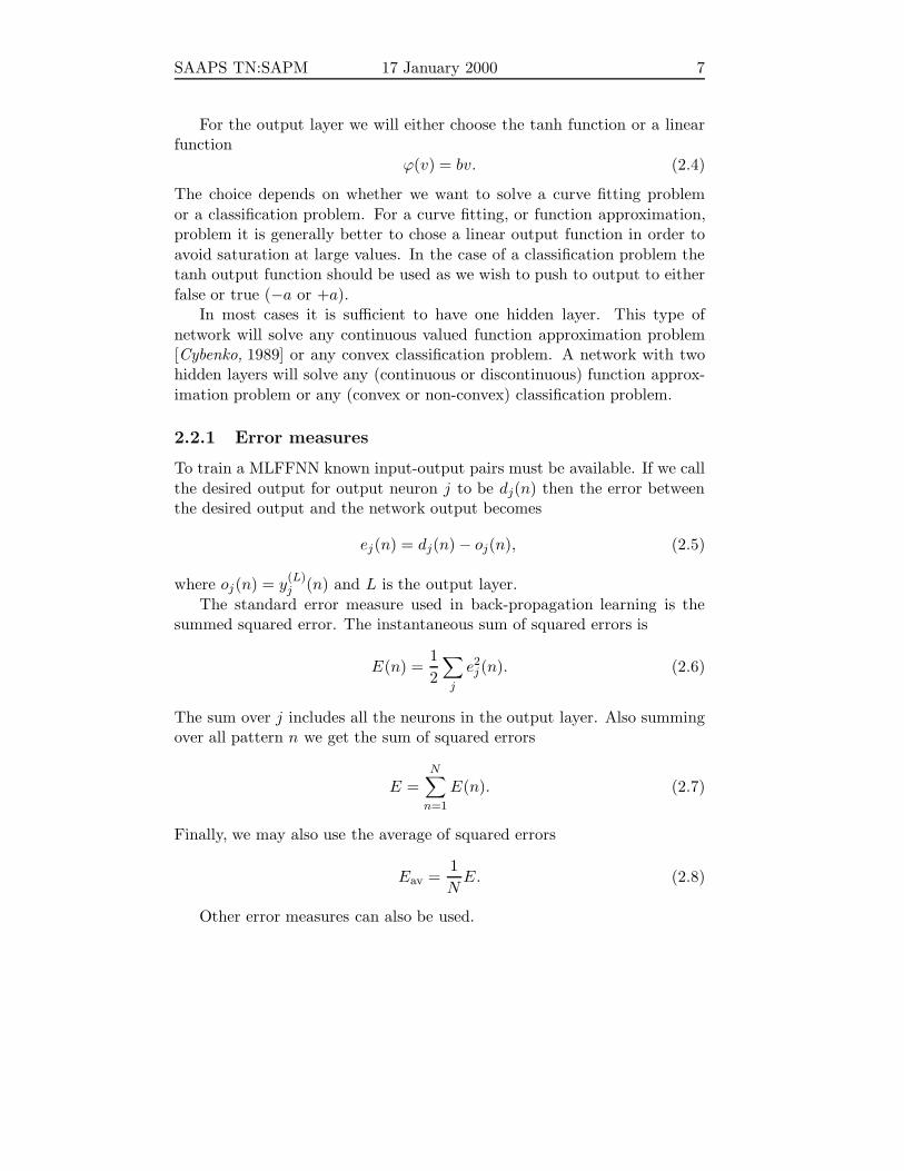
For the output layer we will either choose the tanh function or a linearfunction

ϕ(v) = bv. (2.4)

The choice depends on whether we want to solve a curve fitting problemor a classification problem. For a curve fitting, or function approximation,problem it is generally better to chose a linear output function in order toavoid saturation at large values. In the case of a classification problem thetanh output function should be used as we wish to push to output to eitherfalse or true (−a or +a).

In most cases it is sufficient to have one hidden layer. This type ofnetwork will solve any continuous valued function approximation problem[Cybenko, 1989] or any convex classification problem. A network with twohidden layers will solve any (continuous or discontinuous) function approx-imation problem or any (convex or non-convex) classification problem.

2.2.1 Error measures

To train a MLFFNN known input-output pairs must be available. If we callthe desired output for output neuron j to be dj(n) then the error betweenthe desired output and the network output becomes

ej(n) = dj(n)− oj(n), (2.5)

where oj(n) = y(L)j (n) and L is the output layer.

The standard error measure used in back-propagation learning is thesummed squared error. The instantaneous sum of squared errors is

E(n) =12

∑j

e2j (n). (2.6)

The sum over j includes all the neurons in the output layer. Also summingover all pattern n we get the sum of squared errors

E =N∑

n=1

E(n). (2.7)

Finally, we may also use the average of squared errors

Eav =1NE. (2.8)

Other error measures can also be used.


2.2.2 Back-propagation learning

The goal of the error-back-propagation algorithm is to minimize the errorE by adjusting the weights wji. This is achieved by changing the weightsso the that the error gradient ∂E/∂wji is negative. As the error is onlyknown at the output layer, the errors have to be back-propagated throughthe preceding layers to be able to calculate an error gradient. The weightsare updated according to

w(l)ji (n+ 1) = w(l)

ji (n) + ∆w(l)ji (n), (2.9)

where∆w(l)

ji (n) = ηδ(l)j (n)y(l−1)

i (n) + α∆w(l)ji (n− 1). (2.10)

Here η is the learning coefficient and α is the momentum term. The localgradient δ(l)j (n) is

δ(L)j (n) = e(L)

j (n)ϕ′(v(L)j (n)) (2.11)

for a neuron at the output layer L and

δ(l)j (n) = ϕ′(v(l)j (n))

∑k

δ(l+1)k (n)w(l+1)

kj (n) (2.12)

for a neuron at hidden layer l. The prime function for a tanh activationfunction is

ϕ′(v) = ab(1− ϕ2(v)). (2.13)

2.2.3 Back-propagation with adaptive learning coefficient

The standard back-propagation algorithm is slow. To speed things up thelearning coefficient η can be varied during training. The idea is that eachweight should have its own learning coefficient. The coefficient should in-crease when the error gradient ∂E/∂wji is negative, and decrease when thegradient is positive. This can be achieved with

∆ηji(n) =

κ ifSji(n− 1)Dji(n) > 0−βηji(n) ifSji(n− 1)Dji(n) < 00 otherwise

(2.14)

where Sji(n− 1) and Dji(n) are defined as, respectively

Dji(n) =∂E(n)∂wji(n)

(2.15)

andSji(n− 1) = (1− ξ)Dji(n− 1) + ξSji(n− 1) (2.16)

where ξ is a positive constant. The procedure is called the delta-bar-deltalearning rule [Jacobs, 1988].


2.2.4 Marquardt-Levenberg algorithm

Both the standard backpropagation (BP) and the adaptive learning rateBP algorithms may demand long training times. A more efficient train-ing procedure is the Marquardt-Levenberg backpropagation (MBP) algo-rithm [Hagan and Menhaj, 1994]. MBP is an approximation to the Newtonmethod

∆w = −[∇2E(w)]−1∇E(w), (2.17)

where w are the weights and the error function E is the sum of squarederrors (Eq. 2.7). With this error function the terms in Eq. 2.17 can berewritten using the Jacobian matrix. Neglecting higher order terms theNewton method becomes the Gauss-Newton method. MBP is a modificationof the Gauss-Newton method and can be expressed as

∆w = [JT (w)J(w) + µI ]−1JT (w)e(w). (2.18)

The parameter µ is multiplied by a factor β whenever a step would result inan increase of the error function E, and divided by β whenever E decreases.When µ is large the algorithm becomes the steepest descent with learningrate η = 1/µ, and when µ is small the algorithm becomes the Gauss-Newton.

The Jacobian matrix is

J(x) =

∂e1(w)∂w1

∂e2(w)∂w1

. . .∂eN (w)

∂w1∂e1(w)

∂w2

∂e2(w)∂w2

. . . ∂eN (w)∂w2

......

. . ....

∂e1(w)∂wn

∂e2(w)∂wn

. . . ∂eN (w)∂wn

. (2.19)

The number of columns N is equal to the product of the number of trainingexamples Q and the number of layers L, thus N = Q× L. The number ofrows n is equal to the total number of weights in the network.

The advantage of the MBP is the much reduced training time. However,it also demands more memory to store the elements of the Jacobian matrix.We see that the size of the matrix depends both on the number of trainingexamples and the total number of weights.

2.3 Radial basis function neural networks

The radial basis function neural network (RBFNN) is also a feed forwardnetwork, however, the hidden layer neurons use local transformation func-tions instead of the global functions used in the MLFFNN. The network hasthe following expression

F (x) =N∑

i=1

wiϕ(‖x− xi‖), (2.20)


where xi, i = 1, 2, . . . , N , are the centres of the radial basis functions ϕ.The norm ‖ · ‖ is taken as the Euclidean length. The activation function isthe Gaussian function

ϕ(r) = exp

(− r2

2σ2

), (2.21)

where σ is the width of the function.

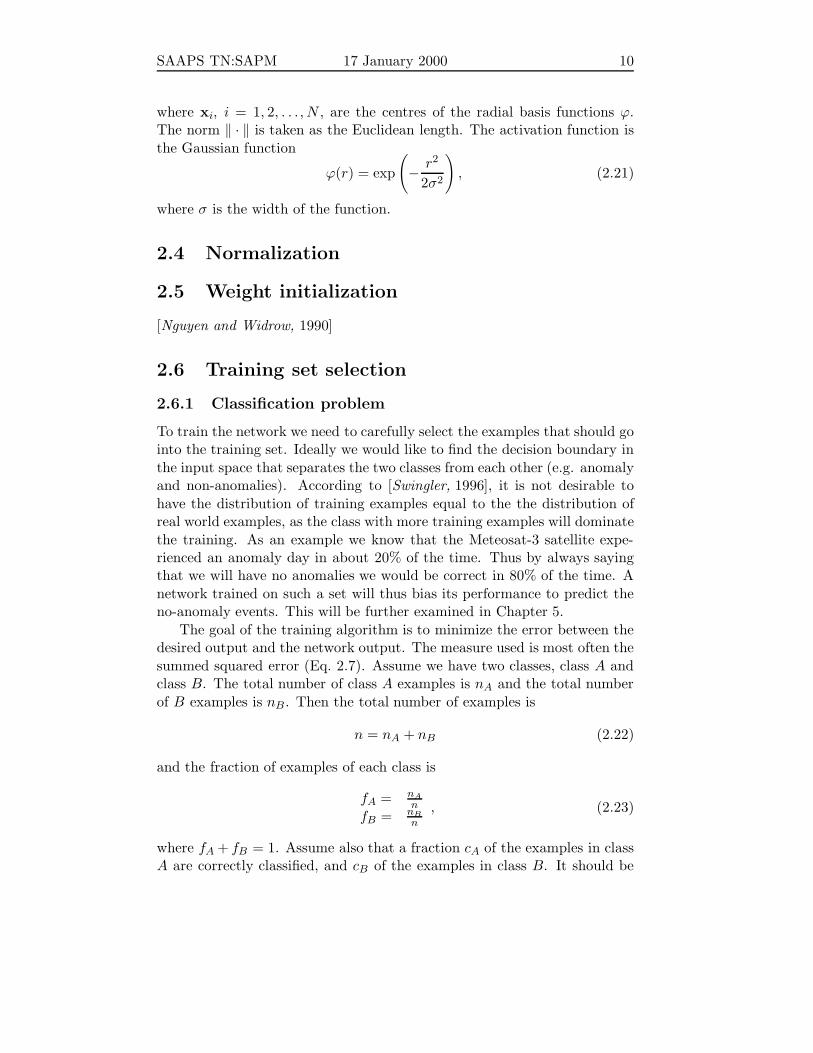
2.4 Normalization

2.5 Weight initialization

[Nguyen and Widrow, 1990]

2.6 Training set selection

2.6.1 Classification problem

To train the network we need to carefully select the examples that should gointo the training set. Ideally we would like to find the decision boundary inthe input space that separates the two classes from each other (e.g. anomalyand non-anomalies). According to [Swingler, 1996], it is not desirable tohave the distribution of training examples equal to the the distribution ofreal world examples, as the class with more training examples will dominatethe training. As an example we know that the Meteosat-3 satellite expe-rienced an anomaly day in about 20% of the time. Thus by always sayingthat we will have no anomalies we would be correct in 80% of the time. Anetwork trained on such a set will thus bias its performance to predict theno-anomaly events. This will be further examined in Chapter 5.

The goal of the training algorithm is to minimize the error between thedesired output and the network output. The measure used is most often thesummed squared error (Eq. 2.7). Assume we have two classes, class A andclass B. The total number of class A examples is nA and the total numberof B examples is nB . Then the total number of examples is

n = nA + nB (2.22)

and the fraction of examples of each class is

fA = nAn

fB = nBn

, (2.23)

where fA + fB = 1. Assume also that a fraction cA of the examples in classA are correctly classified, and cB of the examples in class B. It should be


noted that cA ≤ 1 and cB ≤ 1, and that cA+cB ≤ 2. The fraction of correctclassification then becomes

c = fAcA + fBcB (2.24)= fAcA + (1− fA)cB. (2.25)

This should now be compared with the summed squared error defined inEq. 2.7. Rewriting Eq. 2.7 in terms of the individual contributions from thetwo classes we get

E = EA +EB, (2.26)

whereEA = 1

2

∑n∈nA

(d(n)− y(n))2EB = 1

2

∑n∈nB

(d(n)− y(n))2 . (2.27)

If we assume that we have a tanh transfer function at the output layer thenthe squared error (d(n)− y(n))2 is either 0 for a correct classification or 4for an incorrect classification. Thus if all A classification are wrong thenEA = 1/2nA4 = 2nA. Thus Eq. 2.26 can be written as

E = EA + EB (2.28)= 2nA(1− cA) + 2nB(1− cB) (2.29)= 2n[fA(1− cA) + fB(1− cB)] (2.30)= 2n[fA(1− cA) + (1− fA)(1− cB)] (2.31)= 2n[fA + (1− fA)− fAcA − (1− fA)cB] (2.32)= 2n[1− {fAcA + (1− fA)cB}]. (2.33)

The goal of the training algorithm is to minimize E which, from Eq. 2.33, isidentical to maximizing the total number of correct classifications c. Thus,depending on how we choose fA it will effect the maximum value of c, andalso the values of cA and cB.

2.6.2 Continuous valued problem

2.7 Training strategies

2.7.1 Training, validation and test

The data set that has been created fro the development of the neural networkshould be divided into three subsets: a training set, a validation set, and atest set. The training set is used to train the network, i.e. the process whenthe weights are changed so that the error is minimized. The validation set isused to determine the optimal network with respect to the number of hiddenneurons and the selection of input parameters. It can also be used to decidewhen to stop training. Finally, when the optimal network has been selected


it can then be tested on the test set to find the performance that can beexpected in a real situation. The three sets should not have any overlappingexamples. The sets should also have similar statistics.

The three sets should contain a sufficient number of examples so thatthe network can be properly trained, validated and tested. The numberof examples needed is problem related; a small simple network needs fewerexamples than a large complex network.

2.7.2 Training with minimum set size

Sometimes it is not possible to divide the data set into the three sets be-cause the set is to small. Instead one can use only a training set andthen estimate the size of the network that will generalize well given thesize of the data set and the performance of the network. According to[Baum and Haussler, 1989] a binary classifying network (output 0 or 1) withone hidden layer will almost certainly provide good generalization if thenumber of examples in the training set N satisfies

N ≥ 32Wε

ln32Mε

(2.34)

where W is the number of weights in the network and M is the numberof hidden neurons. If ε is small then the network performs very well onthe training set. If the training set is small (N small) it is probable thatthe network simply has memorized the data and will thus generalize poorly.On the other hand if N is large it is likely that the network has found theunderlying general relationship. Equation 2.34 represents the worst-caseformula for estimating the training set size. In practice it seems that it issufficient to keep the first term and dropping the constants [Haykin, 1994]so that we get

N >W

ε. (2.35)

We can now illustrate equations 2.34 and 2.35 with the anomalies on Meteosat-3. During its operation the satellite experienced about 700 anomalies. Ifwe assume a network with 10 input units (e.g.

∑Kp over 10 days) and 10

hidden units then M = 10 and W = (10 + 1)× 10 + 10 + 1. The minimumnumber of examples needed as a function of ε/2 would vary according toFigure 2.1. Using the criterion from Equation 2.34 we see that N should bemuch larger than the 700 available examples, thus it can not be guaranteedthat the network will generalize. Using the relaxed criterion (Eq. 2.35) wenow see that the Meteosat-3 anomaly set is sufficiently large to be used fortraining when the fraction of errors (ε/2) are larger than 0.1.


0.001 0.005 0.01 0.05 0.1 0.510

2

103

104

105

106

107

108

ε / 2

N

N > 32W/ε ln (32M/ε)N > W/ε

Figure 2.1: The minimum number of examples (N ) as a function of thefraction of errors (ε/2) for a network with 10 input units and 10 hiddenunits.

Chapter 3

Fuzzy systems

14

Chapter 4

Prediction of the electronflux from solar wind data

As described in section 1.1, past attempts to predict the electron flux atgeosynchronuous orbit has always used the local electron flux and/or geo-magnetic indices (Kp, Dst). The emphasis has been on high energies (MeV)which are believed to give internal charging.

As it is the solar wind that drives magnetospheric activity it is naturalto develop models to predict the electron flux using solar wind data. Asthe electron flux can vary by several orders of magnitude within 24 hoursthe time resolution of the predictions should be better than one day. If atime resolution of one hour is used the diurnal variation is captured. At thesame time we avoid difficulties associated with substorm dynamics and theevolution of the solar wind from L1 to the Earth.

As the satellite measures the electron flux at a single point and at thesame time moves in the 24-hour orbit around the Earth, it is not possible todistinguish between spatial and temporal variations. This problem can besolved in two ways: (1) The input is the solar wind data with 24 differentnetworks predicting the flux in each local time sector; (2) The input is thesolar wind data and the local time, and only one network predicting theflux in all local time sectors. It is difficult to say which method will workbest. The first method produces simpler networks as each network onlyhas to model one time sector. However, the training procedure is morecomplicated as 24 networks need to be trained. The number of availabletraining examples will also be reduced by a factor of 24. The second methodwill produce a more complex network as it also has to model the local timevariation. The training procedure is simpler, only one network, but the finalprediction accuracy might be poorer as a collection of simpler specializednetworks usually perform better than one general network. Both approachesshall be examined. The first approach is also similar to the hybrid neuralnetwork [Haykin, 1994].

15


80 85 90 95 100 105 110−10

0

10

Bz

GS

E

80 85 90 95 100 105 1100

10

20

30

Den

sity

80 85 90 95 100 105 110300

400

500

600

Vel

ocity

80 85 90 95 100 105 1100

2

4

x 105

Days from 1 January 1998

E−

flux

Figure 4.1: The solar wind magnetic field (Bz), density, velocity, and the> 0.6 MeV electron flux over 30 days in 1998.


4.1 GOES > 0.6 MeV

4.2 GOES > 2 MeV

4.3 LANL SOPA 50-75 keV







Chapter 5

Prediction of satelliteanomalies

The prediction of satellite anomalies is a binary yes/no-problem, or a clas-sification problem. This can be compared to the prediction of the electronflux which is a continuous valued problem. The prediction of an anomaly iseither completely correct or completely wrong.

Essentially one would like to find a parameter space that can be separatedinto two classes that corresponds to anomaly and no-anomaly, respectively.

5.1 Daily predictions

5.1.1 Meteosat-3 anomalies predicted using∑

Kp

As the daily average electron flux has been predicted using∑Kp it is nat-

ural to develop an anomaly prediction model also using∑Kp. This was

examined by [Wu et al., 1998]. The analysis will be repeated here, however,the definition of anomaly and non-anomaly will be slightly different. If oneor several anomalies occur during a day, then that day is an anomaly day.If no anomalies occur during a day, that day is considered a non-anomalyday.

During the satellites 7 year lifetime (1988-1995) it experienced 724 anoma-lies. The anomalies were spread over 497 days, which should be comparedto the total number of 2678 days for this period. The fraction of days withanomalies were thus 0.19. On average there were a day with anomalies every5.4 days.

Using superposed epoch analysis one can discover trends in Kp thatprecede the anomalies. Figure 5.1 shows how the 3-hour Kp starts increase6 days before the anomaly and reaches the maximum value one day ahead.However, one should also note the large variation of Kp for individual eventsas indicated by the standard deviation (dashed lines).

18


−10 −8 −6 −4 −2 0 2 4 6 8 100.5

1

1.5

2

2.5

3

3.5

4

4.5

5

5.5

Days

Kp

Figure 5.1: The 3-hour Kp superposed on anomaly events from Meteosat-3.The solid line shows the superposed values and the dashed lines are thestandard deviation.


As was shown in Section 2.6 the minimization of the summed squarederror is identical to maximizing the fraction of correct predictions c. Theproblem is to select a suitable training set as the number of days withanomalies is smaller than the number of days without anomalies.

To examine the effect of choosing the training and test sets with differentdistributions we construct a network with 8 input units, 3 hidden units and1 output unit. The inputs are 8 days of

∑Kp and the output is whether

there is an anomaly or not the next day. This network size produced similarerrors on both the training set and the test set. A larger network alwaysled to very small errors on the training set and larger errors on the testset. The total number of training examples has been fixed to ntr = 497and then the fraction of anomalies in the training set f tr

A has been variedover 0.1, 0.2, 0.3, 0.4, 0.5. This means that the number of anomalies in thetraining set ntr

A has been 49, 99, 149, 198, 248. Then the networks have beentested on the test set where also the fraction of anomalies f ts

A have beenvaried over 0.1, 0.2, 0.3, 0.4, 0.5. The result is shown in Figure 5.2. Whenwe have a balanced training set (f tr

A = 0.5) then the fraction of correctclassifications is close to constant (cts ≈ 0.65) independent of the test setdistribution (f ts

A ). When the training set is unbalanced (f trA < 0.5) makes

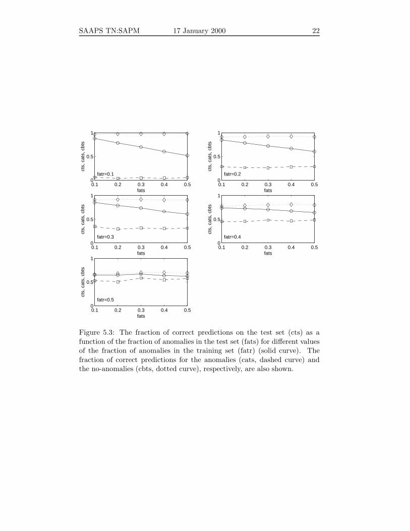
cts dependent on the test set distribution, where cts increases for decreasingf tsA . The result is repeated in Figure 5.3 where each panel shows the varia-

tion of cts as a function of f tsA for constant f tr

A . The solid-circle curves arethe slices for constant f tr

A from Figure 5.2. Also shown in the figure are thefractions of correct classifications for anomalies (ctsA, dash-square curve) andno-anomalies (ctsB dot-diamond curve), respectively. For the balanced train-ing set cts ≈ ctsA ≈ ctsB. This we can understand from the training procedurewhich minimizes E (Eq. 2.7) or equivalently maximizes

ctr = f trA c

trA + f tr

B ctrB . (5.1)

As f trA = f tr

B both cA and cB will be maximized with equal weights. Withan unbalanced training set cA and cB will be maximized unevenly, and iff trA < f

trB then the training algorithm will bias toward maximizing cB. This

is seen in Figure 5.3 and is mostly pronounced for the case when f trA = 0.1.

5.2 Hourly predictions


0.1

0.2

0.3

0.4

0.5 0.1 0.15 0.2 0.25 0.3 0.35 0.4 0.45 0.5

0.5

0.55

0.6

0.65

0.7

0.75

0.8

0.85

0.9

fatsfatr

cts

Figure 5.2: The fraction of correct predictions on the test set (cts) as afunction of the fraction of anomalies in the training set (fatr) and the fractionof anomalies in the test set (fats).


0.1 0.2 0.3 0.4 0.50

0.5

1

fats

cts,

cat

s, c

bts

fatr=0.1

0.1 0.2 0.3 0.4 0.50

0.5

1

fats

cts,

cat

s, c

bts

fatr=0.2

0.1 0.2 0.3 0.4 0.50

0.5

1

fats

cts,

cat

s, c

bts

fatr=0.3

0.1 0.2 0.3 0.4 0.50

0.5

1

fats

cts,

cat

s, c

bts

fatr=0.4

0.1 0.2 0.3 0.4 0.50

0.5

1

fats

cts,

cat

s, c

bts

fatr=0.5

Figure 5.3: The fraction of correct predictions on the test set (cts) as afunction of the fraction of anomalies in the test set (fats) for different valuesof the fraction of anomalies in the training set (fatr) (solid curve). Thefraction of correct predictions for the anomalies (cats, dashed curve) andthe no-anomalies (cbts, dotted curve), respectively, are also shown.


References

Andersson, L., L. Eliasson, and P. Wintoft, Prediction of times withincreased risk of internal charging on spacecraft, Workshop on spaceweather, ESTEC, Noordwijk, WPP-155, 427–430, 1999.

Baum, E.B., and D. Haussler, What size net gives valid generalization?,Neural Computation 1, 151–160, 1989.

Cybenko, G., Approximation by superpositions of a sigmoidal function,Math. Control Signals Systems 2, 303–314, 1989.

Hagan, M.T., and M. Menhaj, Training feedforward networks with the Mar-quardt algorithm, IEEE Trans. Neural Netwworks, 5, 989–993, 1994.

Haykin, S., Neural Networks: A Comprehensive Foundation, Macmillan Col-lege Publishing Company, Inc., New York, 1994.

Jacobs, R.A., Increased rates of convergence through learning rate adaption,Neural Networks 1, 295–307, 1988.

Freeman, J.W., T.P. O’Brien, A.A. Chan, and R.A. Wolf, Energetic elec-trons at geostationary orbit during the November 3-4, 1993 storm: Spa-tial/temporal morphology, characterization by a power law spectrum and,representation by an artificial neural network, J. Geophys. Res., 103,26,251–26,260, 1998.

Koons, H.C., and D.J. Gorney, A neural network model of the relativisticelectron flux at geosynchronous orbit, J. Geophys. Res., 96, 5,549–5,556,1991.

Nguyen, D., and B. Widrow, Improving the learning speed of 2-layer neu-ral networks by choosing initial values of the adaptive weights, in Proc.IJCNN, 3, 21–26, 1990.

Stringer, G.A., and R.L. McPherron, Neural networks and predictionsof day-ahead relativistic electrons at geosynchronous orbit, Proceedingsof the International Workshop on Artificial Intelligence Applications inSolar-Terrestrial Physics, Lund, Sweden, 22-24 September 1993, Editedby J.A. Joselyn, H. Lundstedt, and J. Trolinger, Boulder, Colorado, 139–143, 1993.

Stringer, G.A., I. Heuten, C. Salazar, and B. Stokes, Artificial neural net-work (ANN) forecasting of energetic electrons at geosynchronous orbit, inRadiation Belts: Models and Standards, Geophys. Monogr. Ser., vol 97,edited by J.F. Lemaire, D. Heynderickx, and D.N. Baker, AGU, Wash-ington, D.C., 291–295, 1996.

Swingler, K., Applying neural networks: a practical guide, Academic PressLtd, London, 1996.

Wu, J.-G., H. Lundstedt, L. Andersson, L. Eliasson, and O. Norberg, Space-craft anomaly forecasting using non-local environment data, Study ofplasma and energetic electron environment and effects (SPEE), ESTECTechnical Note, WP 220, 1998.

tn sapm 0.2 - lund.irf.se · saaps tn:sapm 17january2000 1 documentstatussheet technical...

Documents