título artículo / títol article: inferential networked control with

Título artículo / Títol article:

Inferential networked control with accessibility constraints in both the sensor and actuator channels

Autores / Autors

Peñarrocha Alós, Ignacio

Dolz Algaba, Daniel

Sanchis Llopis, Roberto

Revista:

International Journal of Systems Science

Volume 45, Issue 5, 2014

Versión / Versió:

Postprint de l’autor

Cita bibliográfica / Cita bibliogràfica (ISO 690):

PEÑARROCHA, I.; DOLZ, D.; SANCHIS, R. Inferential networked control with accessibility constraints in both the sensor and actuator channels. International Journal of Systems Science, 2013, ahead-of-print: 1-16.

url Repositori UJI:

http://hdl.handle.net/10234/88609

September 4, 2012 10:56 International Journal of Systems Science networked˙control

International Journal of Systems ScienceVol. 00, No. 00, 00 Month 20xx, 1–25

RESEARCH ARTICLE

Inferential networked H∞ control with accessibility constraints in both the

sensor and actuator channels.

I. Penarrocha, D. Dolz, R. Sanchis

[email protected], [email protected] [email protected]

Departament d’Enginyeria de Sistemes Industrials i Disseny,

Universitat Jaume I,

Campus de Riu Sec,

12071 Castello, Spain.(Received 00 Month 20xx; final version received 00 Month 20xx)

The predictor and controller design for an inferential control scheme over a network is addressed. A linearplant with disturbances and measurement noise is assumed to be controlled by a controller that communicateswith the sensors and the actuators through a constrained network. An algorithm is proposed such that thescarce available outputs are used to make a prediction of the system evolution with an observer that takesinto account the amount of lost data between successful measurements transmissions. The state prediction isthen used to calculate the control actions sent to the actuator. The possibility of control action drop due tonetwork constraints is taken into account. This networked control scheme is analyzed and both the predictorand controller designs are addressed taking into account the disturbances, the measurement noise, the scarceavailability of output samples and the scarce capability of control actions update. The time-varying samplingperiods that result for the process inputs and outputs due to network constraints have been determined asa function of the probability of successful transmission on a specified time with a Bernoulli distribution. Forboth designs H∞ performance has been established and LMI design techniques have been used to achieve anumerical solution.

Keywords: Networked control, inferential control, networked estimation, linear matrix inequalities

1. Introduction

Networked based Control Systems (NCS) have been studied extensively in recent years due tothe benefits they offer to real control system implementation. However, the use of a network in acontrol loop introduces some negative effects that can degrade the system performance, as packetdropouts, variable sampling intervals and communications delays, as well as communicationconstraints due to its shared nature. The works Chow and Tipsuwan (2001), Ling et al. (2007),Hespanha et al. (2007), Heemels et al. (2010), Gupta and Chow (2010) show and classify thedifferent problems that appear when dealing with process control over networks, describing somepossible solutions, analysis schemes and open problems. One of the main problems when dealingwith control over networks is the delay and dropout between controller and actuator, that leadsto a time-varying delay on the closed loop. Different types of models are used in the literature,that can be classified in continuous time Wen and Zeng (2012), Liu and Yang (2012), discretetime or hybrid event-driven ones Souza et al. (2011), for which different design procedures areproposed. Which model is applied depends on the mechanisms used to sample the output, holdingor resetting the control input Schenato (2009) and the message sending protocols. When boththe measurements and the control actions are sent through a network, the control strategies

This work was supported by MICINN project number DPI2011-27845-C02-02

ISSN: 0020-7721 print/ISSN 1464-5319 onlinec© 20xx Taylor & FrancisDOI: 10.1080/00207721.20xx.CATSidhttp://www.informaworld.com


2

presented in the literature can be classified in state feedback, output feedback or observer basedstate feedback control. In the first and second strategy the control actions are only updated (or,at least, sent) when a measurement of the full state or the output, respectively, is available. Inthe observer based approach, the control actions are updated (or, at least, sent) independentlyof the output sampling mechanism. The control goals also differ between some works that onlydeal with the stability of the closed loop (neglecting the disturbances), and other ones that takeinto account the presence of state disturbances and some kind of performance optimization iscarried out with H∞ or guaranteed cost control strategies.In recent years, a significant attention has been paid to observer based networked control

systems. In Yang et al. (2006), Luan et al. (2011), Guo et al. (2012), Liu and You (2012) anobserver based control for a NCS was addressed assuming delays on both the input and outputchannel.In Wang et al. (2007), Li et al. (2010), Liu et al. (2011) an observer based control approach

for NCS is proposed where the received measurements as well as the applied control actionsare driven to zero when communication fails. Those approaches make use of the most probablemeasured output and input in the state estimation procedure assuming independent Bernouillidistributions on the input and output packet dropout phenomena and, with this technique, theenlargement of the state vector is avoided. The design of the observer based controller is carriedout off line, while in Hristu-Varsakelis and Zhang (2008) the control action computation is doneonline through an LQG strategy that was latter generalized in the paper Moayedi et al. (2011).In this work, both the reset and zero order hold strategies are addressed, as well as differentapproaches related to the acknowledgement on the success on packet transmissions.In Zhang and Yu (2007) the problem of input packet dropout was dealt with a zero order

hold approach, and a polyquadratic approach was used to assure the stability of the closed loopsystem. In Fang and Wang (2008), Che et al. (2010), Wen et al. (2011) this problem was dealtassuming a stochastic Bernoulli distribution of the packet dropouts and state disturbances on themodels, but the measurement noise was assumed to be null. The controller and the observer wereobtained simultaneously via an LMI procedure, leading to constant gains on the observer and thecontroller that are applied at each control period with the available (possibly) delayed outputs.In Yu et al. (2009) the idea of a varying gain depending on the last transmission interval (the timeelapsed between the last two successfully sent control actions) was introduced. This has beenrecently extended in Shi and Yu (2011), Wang et al. (2011) where a Markovian characterizationof the time-varying delays is done, and where the disturbances have been considered but again,the measurement noise has been neglected.The input channel network-induced delay has been addressed recently through different pre-

diction strategies Gonzalez et al. (2011, 2012) trying to compensate the delay. In Ishido et al.(2011), Xia et al. (2011), Yang et al. (2008) the strategy is based on sending a packet withconsecutive predicted inputs to a buffer located on the actuator side, that decides which inputmust apply taking into account the possible input packet dropout. The study of observers forthe scenario presented in this work has been initially addressed in Penarrocha et al. (2012a) withan online approach, and in Penarrocha et al. (2012b) with an offline approach.For the knowledge of the authors, the off line design of an observer based control approach for

systems with time delay and packet dropout in both channels using a zero order hold approachhas not been considered taking into account the measurement noise phenomena.When dealing with noisy sensors, in the observer based NCS approach, the observer gains must

be fitted depending on the availability of output measurements in order to extract and filter moreefficiently its information. Furthermore, the effect of the noise over the state estimation errorshould be taken into account in the predicted state feedback approach in order to smooth theoutput.In this work, the design of an observer based control strategy for systems with state distur-

bances and measurement noise, controlled through a network, is addressed, assuming data drops


3

Process✲ ✲Actuators Sensors

✻

ZOH

❄✻

↑ U Y ↓✻

❄

Constrainted Network αy[t]αu[t]

Controller

InputBuffer

Output

T T

u[t]y[t]

y(τ)u(τ)

❄❄wc(τ) v(τ)

Buffer

uk

✛

✻

u∗[t] ys

The plant

synchronized ✲✛

Figure 1. Proposed control scheme using a network with variable accessibility constraints. A solid line denotes continuouslytransmitted signals, a dashed line denotes a periodically transmitted signal and a dotted line denotes an arbitrarily on timetransmitted signal

due to accessibility constraints and transmission delays in both channels, sensors to controllerand controller to actuators. The observer has a time varying gain that depends on the consecu-tive measurement packet dropouts, and the state estimation error is taken into account in theH∞ controller design. The sensors, actuators and controller are assumed to be time driven, andthe probability of successful access to the network from the nodes is assumed to be defined by aBernoulli distribution that can also be slowly varying with time. The disturbance attenuation,as well as the probability of dropped data is taken into account in the design of the observerand the controller. As the state is not assumed to be measured, an observer is designed to im-prove the results of previous works, taking into account disturbances and measurement noise,and the knowledge of new measurements reception. An observed state feedback controller isthen designed taking into account the state uncertainty due to the use of an observer. The ideacan be easily extended to the design of full state feedback controllers with state measurementnoise. The main contributions are the consideration of measurement noise, and the use of anoff line calculated time varying gain in the observer, that depends on the elapsed time betweenconsecutive received measurements.The paper is organized as follows. In Section 2 the problem is presented, including the plant

description, a proposal of the network message protocol for control purposes, and the samplingscenario resulting from the network operation. In section 3, the predictor-based (inferential)control algorithm is proposed, and, in section 4, the closed loop dynamics is analyzed. In section5 the predictor is designed, and the controller design is addressed in section 6. In section 7 severalexamples are shown and, finally, the main conclusions are summarized in Section 8.

2. Problem statement

Figure 1 shows the proposed networked control problem with a plant with input and outputinterface devices, a controller, and a network that allows the communication between controllerand process signals. The networked control scheme is described as follows.


4

2.1. Plant description

The plant is assumed to be a continuous-time process with several control inputs (u(τ)) appliedby some actuators and several controlled outputs (y(τ)) measured by some sensors. The processbehaviour is assumed to be defined by the dynamic equations

x(τ) = Acx(τ) +Bcu(τ) +wc(τ) (1a)

y(τ) = C x(τ) + v(τ) (1b)

where all the signals are continuous-time, being u(τ) ∈ Rnu the input of the process, y(τ) ∈ R

ny

the output measured by a noisy sensor, x(τ) ∈ Rn the state, wc(τ) ∈ R

n the process disturbanceand v(τ) ∈ R

ny the sensors measurement noise. Ac, Bc and C are matrices of proper dimensions,where the pair (Ac,C) is assumed to be detectable and the pair (Ac,Bc) is assumed to becontrollable.The input signals of the actuators, u(τ), are updated every T seconds through a zero order

holder (ZOH) with the value of each correspondent u[t] contained in a packet that is stored onan unitary buffer (denoted by ↑ U on the figure).That buffer can be accessed via a network at any arbitrary instant of time in order to update

the packet stored in it. The sensors measurements are sampled every T seconds and all thesampled values (y[t]) are encapsulated in a packet and written on a unitary buffer (Y ↓ on thefigure), that can be accessed by the network at any arbitrary instant of time. It is assumed thatboth the sampler and the zero order holder are synchronized and, therefore, the input updateand the output sample occur at the same time. Based on this assumption, an equivalent sampleddata model of (2) at period T can be written as

x[t+ 1] = Ax[t] +Bu[t] +w[t] (2a)

y[t] = Cx[t] + v[t] (2b)

where all the signals are discrete-time sampled data signals, being u[t] = u(tT ) the con-trol inputs, y[t] = y(tT ) the sampled outputs, x[t] = x(tT ) the discrete state, w[t] =∫ (t+1)TtT

eAc(T−τ)wc(τ)dτ the equivalent discrete process disturbance and v[t] = v(tT ) the sensormeasurement noise at time tT . A, B and C are matrices of proper dimensions that can beobtained from the matrices of the continuous model by

A = eAcT , B =

∫ T

0eAc(T−τ)Bcdτ. (3)

2.2. Network message protocol for control purposes

The controller, sensor nodes and actuators share the information through a network This networkis assumed to be shared with other devices that are not shown in the control scheme, and so,the controller can not always access the network at the desired instants of time (there areaccessibility constraints). However, once the network is accessed by a node, it is assumed thatthe message is sent, without drops or errors, and the transmission delay is varying but boundedby τm < T . The following times are defined: T : The basic control period. τc < T : The controlactions computation time. τs < T : The maximum time that takes all the sensors to make ameasurement. τm < T : The maximum time needed to complete the transmission of a messageonce the network is accessed. τca: The time elapsed since the controller starts trying to accessthe network to send the message with the packet control inputs, till the message actually startsto be sent to the input buffer. τsc: The time elapsed since the output buffer starts trying to


5

access the network to send the message with the packet output measurements, till the messageactually starts to be sent to the controller.When the control actions have been calculated (τc seconds after the interrupt start at τ = tT ),

the controller tries to send a message to the control input buffer through the network with thevalues of the inputs (u∗[t+ 1]). The controller keeps trying to send the message until it is sent,or until the time spent is larger than τca,max = T − τc − τm. In that case, the control actions arediscarded (i.e. u[t+1] = u[t]), and the controller stops trying to send the message until the nextcontrol period. An input availability factor αu[t] is defined that takes values 0 or 1 depending onthe successful inputs transmission. In the case the message is discarded, αu[t] = 0. If the messagecan be sent, the actuators input buffer is updated and the applied inputs at period t + 1 areu[t+ 1] = u∗[t+ 1], and αu[t] = 1. This means that the controller knows which are the appliedinputs at every time.The operation to read a package with the sampled outputs values is different, since it is the

input buffer who tries to send the measured values to the controller. Once the sensors haveobtained the measurement, and they have been encapsulated in a single packet and stored inthe input buffer, the input buffer keeps trying to send the message with the output values to thecontroller during the interval T − τs − τm, while there is time for the message to arrive to thecontroller before the next sampling instant. If the message has not been sent in this time, theinput buffer discards the full packet and stops trying to send the message until a new packet isstored. An output availability factor αy[t] is defined that takes values 0 or 1 depending on thesuccessful outputs transmission. At instant t+1, if the controller has received the measurements,y[t], it stores them and defines αy[t] = 1, otherwise αy[t] = 0 and the outputs are assumed tobe lost (due to drop out or to the impossibility of the input buffer to access the network).With the previously described operation mode, the access restriction and time-varying

network-induced delay effects on the networked control system are transformed into a prob-lem of controlling a process with randomly missing synchronous measurements with constantdelay, and with random, sporadic but synchronous inputs updates, avoiding the design of acontrol system with time-varying delays.Note that the message transmission delay and network accessibility constraints depend on the

network, not on the controller algorithm, but the time dedicated to establish communicationwith the sensors and actuators is limited by the control period T . This means that if a lowcontrol period T is selected, then the probability of having output samples and input updatesat the required time will also be low. This implies that the selection of the control period mustbe a compromise between the closed loop response time of the process and the time needed totransmit the messages (that depends on the network traffic) in order to have a sufficient numberof successfully transmitted output samples and input updates.On the next section, the time-varying sampling period distribution and time-varying input

update period distribution that result from the network access constraints are bounded as afunction of the probability of having a successful output and input transmission, respectively.

2.3. Sampling scenario that results from the network operation

Let us define βy as the controller’s probability of receiving a packet with the output measurementsy[t], i.e. as the probability that τsc < T − τs − τm. In terms of the output availability factor thisis expressed as:

βy = P (αy[t] = 1). (4)

Note that the complementary probability of failing on receiving the output samples is P (αy[t] =0) = 1− βy.Let us also define βu as the actuators probability of receiving an input update u[t], i.e., as the


6

probability that τca < T −τc−τm. In terms of the input updating success factor this is expressedas:

βu = P (αu[t] = 1), (5)

and the complementary probability P (αu[t] = 0) = 1− βu.

These probabilities are not equal in general, and do not depend only on the network operation(delays and access restrictions), but also on the selected control period T . Both probabilities areassumed to be slowly time-variant (due to changes in network traffic), but lower bounded byvalues βu,min and βy,min that represent the worst expected network behaviour.Note also that those probabilities can be modified by the user if the period T is changed

during the controller operation. This can be useful if some degradation on the state estimatoror in the output behaviour is detected. In this sense, a strategy to change the period onlinecould be developed in order to maximize the performance of the controlled system. In this work,however, this idea is not addressed and the changes on the probabilities βu and βy are assumedto be related only to network changes due to its shared nature.With the proposed network operation mode, the s-th sampled outputs are available at a

certain instant t = ts (when the transmission can be completed). The number of basic controlperiods between two consecutive measurements received by the controller at instants ts−1 andts is denoted with Ns, being Ns = ts − ts−1.Following the same previous idea, for the inputs update a similar definition is proposed. tk is

the instant when the k-th inputs update takes place, while Nk is defined as the number of basicperiods between two consecutive control inputs received by the actuators at instants tk and tk+1,i.e. Nk = tk+1 − tk.Both values Ns and Nk vary randomly with time. Their distributions are a function of the

probabilities βy and βu, associated to the availability factors αy[t] and αu[t], respectively. Thesefactors are assumed to be binomial independent variables, such that P{αy[t] = 1} = βy,P{αu[t] = 1} = βu . The probability of Nk to be equal a given value N can be calculatedas the probability of having N − 1 consecutive values of αu = 0 and then one value αu = 1,leading to the equation

P{Nk = N} = P

{N−1⋂

i=1

(αu[t+ i] = 0) ∩ (αu[t+N ] = 1)

}

=(1− βu)N−1βu. (6)

that is also valid changingNk byNs and βu by βy. The above function is monotonically decreasingin N , i.e., the lower the N , the higher the probability. The next result allows to obtain aprobabilistic bound on the values of Ns and Nk based on this equation.

Lemma 2.1: Let α[t] be a binomial variable with P{α[t] = 1} = β. Let us call Nj ∈ N (j canrefer either to k or s) the number of periods between two consecutive instants when α = 1. Fora given ε ∈ (0, 1), if N is chosen to fulfill

N ≥ ln(ε)

ln(1− β)+ 1, (7)

then, P{Nj > N} ≤ ε.


7

Proof : The probability that Nj is higher than N can be expressed by means of (6), leading to

P{Nj>N}=1−P{Nj ∈{1, . . . , N}}=(1−β)N−1≤ε.

Taking logarithms on the above expression and taking into account that ln(1− β) < 0, expres-sion (7) is obtained. �

Equation (7) will be used in the design procedure to calculate the maximum value of Nk andNs that will be taken into account in the design equations. The selection of a sufficiently lowvalue of ε will guarantee that the probability of having a larger Nk or Ns is very small. On theother hand, the equation (6) will be used in the design procedure to calculate the probability ofhaving a control input update Nk periods after the last update.

3. Inferential control algorithm proposal

The controller uses the randomly available sampled outputs values received through the networkto estimate the state at the basic control period T , and to predict it one period ahead. With thisprediction, it calculates the control actions for the next period using a state feedback scheme,and tries to transmit the value to the actuators zero order hold buffer. The main difficulty isthat at the time when the control actions are calculated, the controller does not know if thetransmission to the actuators will be possible or not, and hence the controller design must bebased on the probability of successful communication.The controller is programmed to execute a periodical interrupt every T seconds. At the start

of the interrupt, the controller has the following information:

• αy[t− 1] and hence, if y[t− 1] is available or not.

• αu[t− 2] and hence the previously applied u[t− 1].

• αu[t− 1] and hence the values u[t] that are being applied in the current period.

• x[t − 1|t − 2], i.e. the estimation of the previous state with the information of 2 periodsbefore.

The tasks that are scheduled in the interrupt code during time τ ∈ [t · T, (t + 1) · T [ are asfollows:

(1) The values of the sampled outputs of the previous control period (if available) are used toupdate the estimation of the state at the previous control period using the equation:

x[t−1] = x[t−1|t−2] +L[t−1](y[t−1] −Cx[t−1|t−2])αy [t−1], (8a)

where L[t] is a time varying gain that must be designed.(2) The current state (x[t]) is estimated running the model in open loop. Let us call this

estimation x[t|t− 1]:

x[t|t− 1] = Ax[t− 1] +Bu[t− 1]. (8b)

(3) The state at the next period (x[t+1]) is predicted running again the model in open loop.Let us call this prediction x[t+ 1|t− 1]:

x[t+ 1|t− 1] = Ax[t|t− 1] +Bu[t]. (8c)

(4) The control actions for the next period (let us call it u∗[t+1]) are calculated as a function


8

of the predicted state at t+ 1. A standard discrete state feedback controller is used

u∗[t+ 1] = K x[t+ 1|t− 1],

where K is a gain that must be designed to guarantee the stability and an adequatedisturbance attenuation.

(5) The control actions, u∗[t+ 1], are tried to be transmitted to the actuator zero order holdbuffer until τm seconds before the next periodical interrupt, while the sensor buffer tries totransmit the measured outputs, y[t] to the controller. If the outputs have been received,the values y[t] are stored and the output availability factor is set to one, i.e., αy[t] = 1. Ifthey have not been received, then αy[t] = 0. If the control inputs transmission was possible,the input availability factor is set to one and the input values for the next control periodare stored as the calculated ones. If the transmission was not possible, the input valuesfor the next control period are stored as the previous ones (due to the use of a zero orderhold) and the input availability factor is set to zero, i.e.,

u[t+ 1] =

{u[t], αu[t] = 0,u∗[t+ 1], αu[t] = 1.

In summary, the applied control actions can be expressed as a function of the predictedstate as

u[t+ 1] = K x[t+ 1|t− 1]αu[t] + αu[t]u[t], (8d)

with αu[t] = (1− αu[t]).

The time varying gains L[t] and the constant gain K must be designed to guarantee thestability of the observer and the closed loop, and an adequate attenuation of the disturbancesand measurement noise. The first step is to derive the closed loop dynamics equation that resultsfrom combining the process equations with the previous algorithm. This is the purpose of thenext section.

4. Closed loop dynamics analysis

In the next theorem, the time varying matrix that defines the global closed-loop dynamicsis obtained. For this purpose a relationship between the vectors of inputs, states and statesestimation error is established.

Theorem 4.1 : Consider the control scheme shown in figure 1 where the input updates andoutput measurements are synchronously taken every T seconds. Assume that there exists anequivalent sampled-data model given by (2) that defines the dynamic behaviour at the samplinginstants. Then, if a controller is implemented using algorithm (8), the closed loop dynamicbehaviour is defined by equations

x[t+ 1]u[t+ 1]x[t]

= ACL[t]

x[t]u[t]

x[t− 1]

+BCL[t]

w[t]w[t− 1]v[t]

, (9)


9

y[t] = [C 0 0]

x[t]u[t]

x[t− 1]

+ v[t], (10)

where x[t] is the state estimation error defined as

x[t] = x[t]− x[t], (11)

and where matrices ACL[t] and BCL[t] are

ACL[t] =

A B 0

KAαu[t]

(KBαu[t]+αu[t]

)

−KA2αu[t]

0 0 (I −L[t]Cαy[t])A

, (12)

and

BCL[t] =

I 0 0

0 −KAαu[t] 0

0 (I −L[t]Cαy[t]) −L[t]αy[t]

. (13)

Proof : To prove the theorem, first, the state estimation error dynamics is obtained and then,the state and control input evolution are used to obtain the global closed loop dynamics.From the definition of the state estimation error (11), the state estimation can be written as

x[t] = x[t]− x[t]. From equation (2a) the following relationship can be obtained

Ax[t− 1] +B u[t− 1] = x[t]−w[t− 1].

Using these expressions in the state estimation equation (8b) it leads to

x[t|t− 1] = x[t]−Ax[t− 1]−w[t− 1]. (14)

Advancing one period the equation (8a), and using the above expression and equation (2b), theevolution of the state estimation error can be written as

x[t] = (I −L[t]αy[t]C) (Ax[t− 1] +w[t− 1])−L[t]αy[t]v[t]. (15)

Note that this dynamics only depends on the output availability factor αy[t], and does notdepend on the input update availability.The state prediction at instant t+ 1 calculated by (8c) can be rewritten using (14) as

x[t+ 1|t− 1] = A (x[t]−Ax[t− 1]−w[t− 1]) +Bu[t] (16)

Introducing this expression in (8d) to obtain the control action it leads to

u[t+ 1] = K (A (x[t]−Ax[t− 1]−w[t− 1])+Bu[t])αu[t]

+ αu[t]u[t]. (17)


10

Note that this dynamics only depends on the input update availability factor αu[t], and doesnot depend on the output measurement availability.Finally, expressions (15), (17) and the model (2) can be expressed in matrix form as in (9).

�

Remark 1 : The closed loop dynamics obtained on the previous theorem shows that the closedloop behaves as a linear stochastically time-varying system where the dynamic matrix ACL[t]presents a triangular structure.It is important to stress that the estimation error does not depend on the process state

or inputs, nor in the input update availability factor, but only depends on the disturbance,measurement noise and output availability factor as shown in the equation

x[t] = (I −L[t]Cαy[t])(Ax[t− 1] +w[t])−L[t]αy[t]v[t]. (18)

This means that the state observer can be designed independently of the controller to achieve astable behaviour and an appropriate disturbance and noise attenuation level. As a result of theobserver design, a bound in the state estimation error can be obtained.On the other hand, the dynamics of the system state depends on the estimation error of the

designed observer but not on the measurement noise. It can also be noticed that does not dependon the output availability factor. The resulting dynamics can be written as follows:

[x[t+ 1]u[t+ 1]

]

=

[A B

KAαu[t] KBαu[t] + αu[t]

] [x[t]u[t]

]

+

[I 0 0

0 −KAαu[t] −KA2αu[t]

]

w[t]w[t− 1]x[t− 1].

(19)

In Penarrocha et al. (2005), Wu et al. (2011), Gawthrop and Wang (2011) the separationprinciple for observer-based NCS systems that present a triangular structure was demonstrated,leading to an independent design of the observer and the controller gains. Furthermore, thework Wu et al. (2010) demonstrated that the mean square stability of NCS systems with a timevarying model that is only updated when successful transmissions occurs is equivalent to themean square stability at the (fast) control period.The previous results show that both the controller and the predictor can be designed indepen-

dently to have a mean square stable behaviour at their updating periods, and this guaranteesthe mean square stability of the closed loop. They also show that the predictor design musttake into account only the problems with irregular outputs sampling, while the controller designneeds to take into account only the irregular inputs update. As a result, the design strategy isproposed as follows:

(1) Obtain some bound on the disturbance and measurement noises, for example, ‖w[t]‖RMS

and ‖vi[t]‖RMS , i = 1, · · · ny, that will be used in the design steps.(2) Design a stable observer that minimizes the effect of the disturbance and measurement

noise on the state estimation error (18), using the previous bounds and taking into accountthe irregular output sampling (i.e., the dependency on the availability factor αy[t] withprobability βy). This design should give as a result a law for the gain L[t] and a boundon x[t], for example, ‖x‖RMS .

(3) Design a controller to stabilize the system and to minimize the effect of the state estimationerror and disturbances, using the previous norms, and taking into account the non periodicinput update (i.e., the dependency on the availability factor αu[t] with probability βu).For this design, equation (19), where the disturbance vector includes the state estimation


11

error, must be used. The result should be a law for K.

5. Predictor design

In order to design the predictor needed to compute the control actions, the prediction errordynamics is first obtained.

Theorem 5.1 Prediction error dynamics: The prediction error dynamics of the algorithm (8)applied to system (2) when there is no modeling error and the measurements are available everyNs periods (with Ns time variant), is described by the linear time-variant system

xs = (I −LsC)

ANs xs−1 +

Ns∑

j=1

Aj−1w[ts − j]

−Ls vs (20)

that is updated every time new measurements are available. The estimation error vector is definedwhen the measurements are available (t = ts) as xs ≡ x[ts] = x[ts]− x[ts]. The state predictionerror between measurements (from t = ts−1 to t = ts − 1) is given by (r ∈ [0, Ns − 1])

x[ts−1 + r] = Arxs−1 +r−1∑

i=0

Ar−i−1w[ts−1 + i]. (21)

Proof : At the measuring instant ts, the state estimation error in (18) can be expressed (withαy[t] = 1) as

x[ts] = (I −LsC) (Ax[ts − 1] +w[ts − 1])−Lsvs. (22)

being Ls = L[ts] and vs = v[ts]. At the instants when no measurements are available, the stateestimation error evolution is obtained taking αy[t] = 0 in (18)

x[t] = Ax[t− 1] +w[t− 1], ts−1 < t < ts. (23)

Introducing recursively equation (23) from t = ts−1 to t = ts−Ns+1 into (22), it leads to (20)taking into account that ts − Ns = ts−1. Expression (21) can be obtained using recursivelyequation (23) from t = ts−1 + 1 to t = ts−1 + r. �

Remark 1 : Let us assume that Ns is the maximum number of periods between availablemeasurements, i.e., a bound of Ns. Then, if a new vector gathering the disturbances betweenmeasurements is defined as

Ws =[v⊤s w[ts − 1]⊤ · · · w[ts − Ns]

⊤]⊤

,

the prediction error dynamics at measuring instants can be written in a compact way as

xs = As xs−1 +BsWs (24)

where

As = (I −LsC)ANs , (25)

Bs =[−Ls (I −LsC)Λ(Ns)

]

n×(1+Nsn)(26)


12

being Λ(Ns) the matrix defined as

Λ(Ns) = [

Ns

︷︸︸︷

I A A2 · · · ANs−1 0 · · · 0︸︷︷︸

Ns

] (27)

The state estimation error dynamics at the inter-sampling periods (21) can also be compactedas

x[ts−1 + r] = Arxs−1 + F (Ns, r)Ws, r ∈ [0, Ns − 1] (28)

where F (Ns, r) is a n× (1 + Nsn) matrix defined by

F (Ns, r) = [0n×1 0 · · · 0r

︷︸︸︷

I A · · · Ar−1︸︷︷︸

Ns

0 · · · 0]. (29)

The observer dynamics depends on the vector gain Ls defined at measuring instants (t =ts), that must be designed to assure: the predictor stability, robustness to the irregular dataavailability and a proper attenuation of the disturbances and measurement noises. One possibleapproach is online gain calculation (Kalman filter approach), but this would not lead to any apriori information about achievable bounds on the state estimation error (as expected in theproposed strategy in Remark 1). Furthermore, a high online computational effort is neededbecause a stationary state can not be reached. Therefore, an off line gain scheduling is proposed,trying to find a priori state estimation error bounds, and reducing the online computational costneeded. As the number of periods between consecutive measurements (Ns) can be known online,the design of gain Ls in this work is addressed defining a different gain for each possible valueof Ns. In order to calculate the set of gains Ls off line, an upper bound (Ns) in Ns must beassumed. To calculate that bound, equation

Ns =

⌈lg(ε)

lg(1− βy)+ 1

⌉

. (30)

is used, where ε is chosen to be sufficiently low to guarantee that the probability of havingNs > Ns is very small. The result of the off line calculation is a finite set of gains

Ls = L(Ns) ∈ L = {L(1),L(2), . . . ,L(Ns)}, (31)

and a bound on the norm of the state estimation error (calculated at the basic control period).Every time a new measurement is available, a different gain Ls is applied, depending on thenumber of periods (Ns) that the predictor has been waiting for new measurements.With this approach, matrices As and Bs in (24) can be defined as a function of Ns:

As = A(Ns) = (I −L(Ns)C)ANs , (32a)

Bs = B(Ns) =[−L(Ns) (I −L(Ns)C)Λ(Ns)

](32b)

Theorem 5.2 H∞ observer design: Consider the predictor algorithm defined by equations (8b)and (8a) applied to system (2) and assume that the outputs are available every Ns ≤ Ns periods.


13

For given γv1 , · · · , γvny, γw ∈ R

+, assume that there exist Ns matrices QN ∈ Rn×n, a symmetric

positive definite matrix P ∈ Rn×n, and matrices XN ∈ R

n×ny(with N = {1, . . . , Ns}) such thatthe following LMI fulfills

MA(1) MB(1)⊕Ns

N=1QN +QTN − P

......

MA(Ns) MB(Ns)P −A1 −A2

⋆ ⋆ Γ−A3

≻ 0, (33)

with ⋆ denoting symmetric terms and

MA(N) =√pN (QN −XN C) AN , (34a)

MB(N) =√pN[−XN (QN −XNC)Λ(N)

](34b)

A1 =

Ns−1∑

N=0

pN+1AN⊤

AN ; A2 =

Ns−1∑

N=0

pN+1AN⊤

F (Ns, N),

A3 =

Ns−1∑

N=0

pN+1F (Ns, N)⊤F (Ns, N),

Γ = diag{γv1 , · · · , γvny,1

Ns

γwI},

where pN is the probability of having an outputs sampling period of N , given by pN = (1 −βy)

N−1βy, N = 1, . . . , Ns − 1, and pNs= 1−∑Ns−1

N=1 pN , and matrices Λ(N) and F (Ns, N) aregiven by (27) and (29).Then, defining the predictor gain as LN = Q−1

N XN , the state estimation algorithm definedby (8b) and (8a) converges asymptotically to zero in the absence of disturbances and, underzero initial condition, the RMS norm of the state prediction error, computed at the basic controlperiod, is bounded by

E{‖x[t]‖2RMS} <

ny∑

i=1

γvi‖vi[t]‖2RMS + γw‖w[t]‖2RMS (35)

Proof : The conditions Q⊤N + QN − P ≻ 0 imply that QN are of full rank and P is strictly

positive definite. Therefore the following matrix inequality is fulfilled

(QN − P )⊤P−1(QN −P ) � 0

which is equivalent to

Q⊤NP−1QN � Q⊤

N +QN − P . (36)

Introducing XN = QNLN in (33), taking into account (36) and applying Schur complements


14

one obtains

(∑Ns

N=1 pNA(N)⊤PA(N)−P +A1

)∑Ns

N=1 pNA(N)⊤PB(N) +A2

⋆

(∑Ns

N=1 pNB(N)⊤PB(N)−Γ+A3

)

≺0 (37)

As A1 � 0, inequality (37) implies

x⊤s−1

Ns∑

N=1

pNA(N)⊤PA(N)−P

xs−1 < 0.

Assuming that there are no disturbances or measurement noises, using (24) and (32a), the aboveexpression leads to

E{x⊤s Psxs} − x⊤

s−1Ps−1xs−1 ≺ 0,

which assures mean square stability of the prediction error if the Lyapunov function Vs = x⊤s P xs

is defined.Now, multiplying inequality (37) by

[x⊤s−1W

⊤s

]on the left, and by its transpose on the right,

it leads to

E{Vs} − Vs−1+

Ns−1∑

N=0

pN+1x[ts−1+N ]⊤x[ts−1+N ]−W⊤s ΓWs < 0,

where the predictor dynamic error (24) and open loop prediction error (28) have been taken intoaccount. Assuming a null initial prediction error (x0 = 0) and adding from s = 1 to s = S itleads to

VS +

S∑

s=1

Ns−1∑

N=0

pN+1x[ts−1+N ]⊤x[ts−1+N ]−W⊤s ΓWs

<0. (38)

As P ≻ 0, then VS > 0, leading to

S∑

s=1

Ns−1∑

N=0

pN+1x[ts−1+N ]⊤x[ts−1+N ]−W⊤s ΓWs

< 0. (39)

Introducing the definitions of Γ and Ws it can be written that

S∑

s=1

Ns−1∑

N=0

pN+1x[ts−1 +N ]⊤x[ts−1 +N ]−ny∑

i=1

γvivi[ts]2

− 1

Ns

γw

Ns−1∑

N=0

w[ts−1 +N ]⊤w[ts−1 +N ]

< 0. (40)


15

Dividing by S this expression, and taking the limit when S tends to infinite, the RMS norm ofthe signals at period T is obtained as in (35).

�

The previous result needs the assumption that Ns can not take values above Ns. This is onlytrue if the network can guarantee the output measurements transmission when Ns − 1 periodshave elapsed without any output receptions. If the network can not assure this, but Ns is selectedaccording equation (30), Ns can take larger values, but with a very low probability ε. In thosesporadic cases, the use of the gain calculated for Ns is proposed, i.e. L(Ns) = L(Ns) ∀Ns ≥ Ns.Therefore, the predictor gains can be designed following the previous procedure, but a test forstability that takes into account the unboundedness of Ns is needed. The next result expressesthis stability test.

Theorem 5.3 : Assume that for a given set of matrices L(Ns), the gains L(1), . . . ,L(Ns − 1)are used for the values Ns = 1 to Ns − 1, and the gain L(Ns) is used when Ns ≥ Ns. Assumealso that there exists a symmetric positive definite matrix P ∈ R

n×n such that the followingconditions hold

P −Ns−1∑

i=1

βy(1− βy)i−1AiTX(i)Ai

+ βy(1− βy)Ns−1ANs

⊤QANs ≻ 0, (41)

√

1− βy|λ(A)| < 1, (42)

with

Q = vec−1

{(

I − (1− βy)(A⊤ ⊗A⊤)

)−1vec{X(Ns)

}}

(43)

X(i) = (I −L(i)C)⊤P (I −L(i)C) (44)

then, the observer is stable in the average sense for all the possible sampling scenarios describedby the probability βy (from Ns = 1 to ∞).

Proof : Let us first define the Lyapunov function V(xs) = x⊤s P xs. The expected value of the

Lyapunov function at each instant when new measurements are available depends on the timewhen the previous measurements were available, and is given by

E{V(xs)} = x⊤s−1

Ns−1∑

i=1

βy(1− βy)i−1Ai⊤X(i)Ai+

∞∑

i=Ns

βy(1− βy)i−1Ai⊤X(Ns)A

i

xs−1

if null disturbances are assumed. The second addend can be written as βy(1 −βy)

Ns−1(ANs)⊤QANs , with Q =∑∞

i=0(1 − βy)iAi⊤X(Ns)A

i. The infinity sum Q will onlyresult in a finite value if the eigenvalues of the powered matrices are lower than one, i.e., if√

1− βy|λ(A)| < 1. If this condition is fulfilled, using the encapsulating sum formula, the previ-ous sum can be written as expressed on equation (43). The stability in the average sense will besatisfied if E{V(xs)} < V(xs−1), that is an equivalent condition to that expressed in (41). Note


16

that the expression is an LMI as the vec{·} and vec−1{·} operators keeps the linearity over thedecision variables on matrix P . �

Remark 2 : The condition√

1− βy|λ(A)| < 1 is always fulfilled if the process is open loopstable. However, if the system is unstable, this condition imposes a restriction in the relationbetween the network accessibility and the maximum unstable eigenvalue in order to guaranteethe stabilizability of the closed loop (the lower the network accessibility, the lower the maximumeigenvalue allowed).

In the case that LMI (41) is not feasible, then a lower value of ε, i.e. a larger value of Ns,should be selected to recalculate the predictor gains.

Remark 3 Design procedure: If the norms of the disturbance and noises are known, thenminimizing the sum

ny∑

i=1

γvi‖vi[t]‖2RMS + γw‖w[t]‖2RMS

along LMI (33) will lead to the observer gains set, L(Ns), that minimize ‖x[t]‖RMS . This mini-mization can be solved with standard convex optimization tools.

6. Controller design

Theorem 6.1 :

Consider the controller algorithm defined by equations (8) applied to system (2). Assume thatduring period tk the controller can transmit to the input buffer the value u∗[t + 1]. Then, thestate dynamics of the control system with control algorithm (8) when there is no modelling errorand there is one input update every Nk control periods (with Nk time variant), is described bythe linear time-variant system

x[tk+1+Nk] =

(

ANk+Nk−1∑

i=0

AiBK

)

x[tk+1] (45)

+

Nk−1∑

i=0

Ai (w[tk+Nk−i]−BKξk)

that is updated every time a new input update is available, and being ξk the disturbance contri-bution of the 2-step prediction used on the control action calculation that is given by

ξk = w[tk] +Aw[tk − 1] +A2x[tk − 1]. (46)

Proof : If during the t = tk-th period the input buffer is accessed (αu[tk] = 1), the controlactions that will be applied at period tk + 1 can be written as a function of the state, stateestimation error and disturbances (using the second row on matrices ACL and BCL in (9)) as

u[tk + 1] = KAx[tk] +KB u[tk] (47)

−KA2x[tk − 1]−KAw[tk − 1],

with u[tk] the control action that has been applied since the last input update was available at


17

t = tk −Nk−1. Combining (2a) with (47), it leads to

u[tk+1] = Kx[tk+1]−K(w[tk]+Aw[tk−1]+A2x[tk−1]

). (48)

The evolution of the state from the instant in which the input update is done (tk + 1) until thenext input update occurs (at instant tk +Nk + 1) is given by

x[tk+i] = Ax[tk+i−1] +B u[tk+1] +w[tk+i−1] (49)

where i = 2, . . . , Nk+1 and the control action is the value written on the buffer during period tk(u[tk +1]). Introducing expression (48) in (49) and applying it recursively from i = 2 to i = Nk,it finally leads to (45). �

Remark 1 : If a new vector gathering the disturbances between input updates is defined as

Wk =[w[tk + Nk]

⊤ · · · w[tk + 1]⊤ ξk]⊤

,

with Nk the maximum input update period considered in the control system, then, the systemevolution between input update instants can be written in a compact way as

x[tk + 1 +Nk] = Ak x[tk + 1] +BkWk (50)

(51)

where

Ak = ANk +

Nk−1∑

i=0

AiBK, (52)

Bk =[

Λ′(Nk) −∑Nk−1

i=0 AiBK]

(53)

being Λ′(Nk) the matrix defined as

Λ′(j) = [0 · · · 0

j︷︸︸︷

I A A2 · · · Aj−1︸︷︷︸

Nk

]n×Nkn, (54)

The closed loop system dynamics depends on the matrix gain K that is applied at inputupdating instants (t = tk), and must be designed to assure: the system stability, robustness tothe irregular data availability and a proper attenuation of the state estimation error and thedisturbances.The difference on the controller design with respect to the predictor design is that the controller

does not know in advance when the control inputs will be again updated, or, in other words, howmany periods an updated control input will be applied until the next input update is possible.For this reason, the design of a controller gain that depends on each input updating period Nk

is not possible, and then a constant gain K is proposed1. Taking this into account, matrices Ak

1The dependence on Nk would have been possible if a Markov chain were considered, as in the recent works Yu et al. (2009),Shi and Yu (2011), Wang et al. (2011). This idea will be developed in future work.


18

and Bk can be written as a function of the input update period as

Ak = A(Nk) = ANk +Nk−1∑

i=0

AiBK, (55)

Bk = B(Nk) =[

Λ′(Nk) −∑Nk−1

i=0 AiBK]. (56)

In the controller design, a stochastic strategy that assures the convergence of the control systemin an average sense, depending on the actual value of βu, is proposed.

Theorem 6.2 Stochastic H∞ controller design: Consider the control algorithm (8) applied tosystem (2). Assume that the probability of accessing the input buffer in each control period is βu,but the resulting input updating period is bounded by Nk ≤ Nk, i.e., the priorities of the networkare assumed to be changed to guarantee the control input successful transmission in the case thatNk − 1 periods have elapsed since the last update. For a given γw, γξ ∈ R

+, assume that thereexist symmetric positive definite matrices P ,Q ∈ R

n×n and matrices X ∈ Rnu×n such that

MA(1) MB(1)⊕Nk

N=1 Q...

...MA(Nk) MB(Nk)P − I 0

⋆ Γ

≻ 0, (57)

P Q = I, (58)

where pN is the probability of having an input updating period of N , given by pN = (1−βu)N−1βu,

N = 1, . . . , Nk − 1, and pNk= 1−∑Nk−1

i=1 pN . The matrices are defined as follows

MA(N) =√pN

(

AN +

N−1∑

i=0

AiBK

)

, MB(N) =√pN [Λ′(N) −

N−1∑

i=0

AiBK] (59)

with

Γ = diag{ 1

Nk

γwI, γξI}. (60)

Then, the system is mean square stable in the absence of disturbances or estimation error,and, under zero initial conditions, the state is bounded by

E{‖x[t]‖2RMS} < γw‖w[t]‖2RMS + γξ‖ξ[t]‖2RMS . (61)

Proof : Applying Schur complements to matrix inequality (57) and multiplying by


19

[x[tk + 1]⊤, W⊤

k

]on the left and by its transpose on the right it finally leads to

Nk∑

N=1

pN (A(N)x[tk + 1] +B(N)Wk)︸︷︷︸

⋆

⊤P (⋆)

− x[tk + 1]⊤(P − I)x[tk + 1]

− γw

Nk

Nk∑

N=1

pNw[tk +N ]⊤w[tk +N ]− γξξ⊤k ξk < 0. (62)

If a Lyapunov function is defined as V[t] = x[t]⊤Px[t], the first addend of the previousexpression represents E{V[tk+1 + 1]}, that is the expected value of the Lyapunov function forthe next control period. Then, under zero disturbance and zero state estimation error condition,the convergence in average is assured (E{V[tk+1 + 1]} < V[tk + 1]). Adding the expression (62)from k = 0 to k = K > 0 it leads

K∑

k=0

E{V[tk+1 + 1]} − V[tk + 1] + x[tk + 1]⊤x[tk + 1]

<γw

Nk

K∑

k=0

Nk∑

N=1

w[tk +N ]⊤w[tk +N ] + γξξ⊤k ξk.

Assuming null initial state (x[tk +1] = 0), dividing by K and taking the limit when K tends toinfinite, then (61) is obtained. �

The previous result needs the assumption that Nk can not take values above Nk. This isonly true if the network can guarantee the control inputs transmission when Nk − 1 periodshave elapsed without any input update. If the network can not assure this, but Nk is selectedaccording equation (7), Nk can take larger values, but with a very low probability ε. Therefore,the gain can be designed following the previous procedure, but a test for stability that takes intoaccount the unboundedness of Nk is needed. The next result expresses this stability test.

Theorem 6.3 : For a given controller matrix gain K, if the probability of successful transmis-sion of the control input in each period is βu, a sufficient condition to assure that the closed loopis stable in the average sense in the absence of disturbances and for all the possible samplingscenarios (from Nk = 1 to ∞) is the existence of a symmetric positive definite matrix P ∈ R

n×n

such that the following LMI condition hold

βu(I−K)T vec−1{(I−βuA

T⊗AT )−1vec{ATPA}}(I−K)

+ KTPK+βuSym{KTP (I−βuA)−1A(I−K)

}−P ≺0 (63)

being K = (I −A)−1BK, βu = 1− βu.

Proof : Let us define the Lyapunov function at the instant in which a new control action isupdated as Vk = xTk Pxk. In the absence of disturbances, the expected value of the Lyapunov


20

function in the next instant when a new control action is updated is given by

E{Vk+1}=∞∑

N=1

βu(1−βu)N−1xT

k

AN+

N−1∑

j=0

AjBK

︸︷︷︸

⋆

T

P (⋆)xk

Taking into account that∑N−1

j=0 Aj = (I−A)−1(I−AN ) it follows

E{Vk+1} = xTk

∞∑

N=1

βuβN−1u

(AN

(I−K

)+K

)

︸︷︷︸

⋆

TP (⋆)xk.

If the infinite summation is developed, using the encapsulating sum formula, the following com-pact form can be obtained

E{Vk+1} = xTk

(βu(I − K)Tvec−1

{(I − (1− βu)A

T ⊗AT )−1vec{ATPA}}(I − K)

+KTPK + βuSym{KTP (I − (1− βu)A)−1A(I − K)})xk. (64)

From this expression it is straightforward to show that (63) is equivalent to condition E{Vk+1} <

Vk. �

In the case that LMI (63) is not feasible, then a lower value of ε, i.e. a larger value of Nk,should be selected to recalculate the controller gain.

Remark 2 : If the norms of the disturbance and the estimation error effect of the two-stepprediction ξk are known, then, minimizing the sum γw‖w[t]‖2RMS + γξ‖ξ[t]‖2RMS subject toLMI (57) and (58) will minimize ‖x[t]‖2RMS .The norm of ‖ξk‖2RMS is not previously known but it can be bounded by

‖ξ[t]‖2RMS < ‖I +A‖22‖w[t]‖2RMS + ‖A2‖22‖x[t]‖2RMS , (65)

where the norm of w[t] is assumed to be known, and where the norm of x[t] is the resultingbound on the predictor design.

The optimization problem presented in Remark 2 is not an strict LMI problem due to bilinearequality constraint (58). As stated in El Ghaoui et al. (1997), this kind of nonconvex feasibilitycan be solved using the complementarity linearization algorithm following the next procedure.First, the optimization problem presented in Remark 2 is rewritten as

min trace(PQ)

subject to (57),

γw‖w[t]‖2RMS + γξ‖ξ[t]‖2RMS < γ (66)[P I

I Q

]

� 0 (67)

where γ is a real positive value. The above nonlinear minimization problem, where γ must beminimized, can be solved using the following bisection algorithm over a cone complementarityiterative algorithm.


21

Step 1 Choose a large enough initial γu such that there exists a feasible solution to LMI condi-tions (57), (66) and (67) with γ = γu. Set γl = 0, and set initially γ = 1

2(γl + γu).

Step 2 Set k = 0 and find a feasible solution set [P k,Qk,Kk, γkw, γkξ ], satisfying (57), (66) and (67).

Step 3 Solve the following LMI problem for the decision variables P , Q, K, γw and γξ:

min trace(P k Q+ P Qk)

subject to (57), (66), (67)

set k = k + 1, P k = P , Qk = Q.

Step 4 If k < kmax, for a given prescribed maximum number of iterations kmax, and (57) is notsatisfied after replacing Q by P−1, then return to Step 3. If k < kmax and (57) are satisfied,update the upper bound on γ as γu = γ, store the actual controller gain K, and go to Step5. If k = kmax, update the lower bound on γ as γl = γ and go to step 5.

Step 5 If γu − γl > δ, for a given small δ, update γ with γ = 12(γl + γu) and go to Step 2. If

γu − γl ≤ δ exit with the last stored solution K in Step 4.

7. Example

Consider the 3-input, 3-output, 6th order unstable LTI plant from Hristu-Varsakelis and Zhang(2008) defined by matrices

A =

1.1 0 0 0 0 0−1.5 0 −0.75 −1.5 −0.75 −0.75−1.1 0 0 −1.1 0 00 0 0 1.1 0 01.1 0.75 0 1.1 0 −0.75

−0.75 0 −0.75 −0.75 0 −0.75

,B =

1 0 11 −1 0−1 1 00 0 −11 0 10 −1 0

,

C =

1 0 1 0 0 00 1 0 0 1 −10 0 0 −1 0 0

.

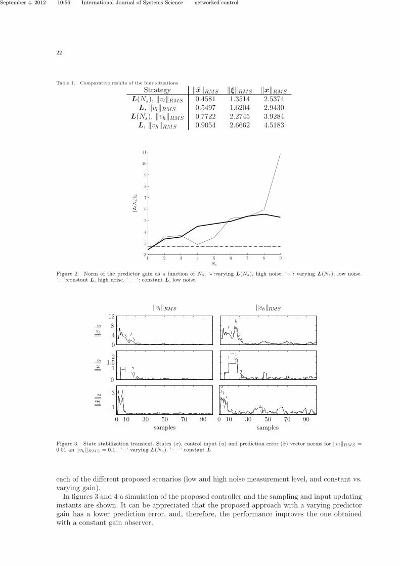
Assume that there is a network where the probabilities of successful transmission of packetscontaining either all data measurements from sensors or all control actions from the controllerare βy = βu = β = 0.6. Assume a disturbance bounded by the norm ‖w‖RMS = 0.01, andtwo different measurement noise levels bounded by ‖vl‖RMS = 0.01 (low) and ‖vh‖RMS = 0.1(high), affecting the three measurements. The maximum number of periods between samples,with a probability of 1 − ε = 0.999 results to be Ns = Nk = 9. Two strategies are comparedfor both noise levels, a constant predictor gain L and a varying one depending on the samplingperiod Ls = L(Ns) (Ns = 1, . . . , 9). Following the results in section V and VI, the boundson the prediction error ‖x‖RMS , on the two-step prediction error ‖ξ‖RMS and on the statetracking error ‖x‖RMS are obtained, as well as the predictor and controller gains. Both theLMI (41) and (63) are feasible with the computed gains and, therefore, stability is guaranteed.Table 1 shows the errors RMS norm. It can be appreciated how the use of a varying predictorgain depending on the sampling period, allows to decrease the state tracking error ‖x‖RMS inapproximately 15% for both low measurement noise and high measurement noise. Figure 2 showsthe norms of the predictor gains as a function of the number of periods between samples, Ns for


22

Table 1. Comparative results of the four situations

Strategy ‖x‖RMS ‖ξ‖RMS ‖x‖RMS

L(Ns), ‖vl‖RMS 0.4581 1.3514 2.5374L, ‖vl‖RMS 0.5497 1.6204 2.9430

L(Ns), ‖vh‖RMS 0.7722 2.2745 3.9284L, ‖vh‖RMS 0.9054 2.6662 4.5183

Ns

‖L(N

s)‖

2

1 2 3 4 5 6 7 8 92

3

4

5

6

7

8

9

10

11

Figure 2. Norm of the predictor gain as a function of Ns. ’-’:varying L(Ns), high noise. ’−’: varying L(Ns), low noise.’.−’:constant L, high noise. ’−−’: constant L, low noise.

‖x‖ 2

‖vl‖RMS

‖u‖ 2

samples

‖x‖ 2

‖vh‖RMS

samples

0 10 30 50 70 900 10 30 50 70 90

1

3

0

11.52

0

4

8

12

Figure 3. State stabilization transient. States (x), control input (u) and prediction error (x) vector norms for ‖vl‖RMS =0.01 an ‖vh‖RMS = 0.1 . ’−’ varying L(Ns), ’−−’ constant L

each of the different proposed scenarios (low and high noise measurement level, and constant vs.varying gain).In figures 3 and 4 a simulation of the proposed controller and the sampling and input updating

instants are shown. It can be appreciated that the proposed approach with a varying predictorgain has a lower prediction error, and, therefore, the performance improves the one obtainedwith a constant gain observer.


REFERENCES 23

Ns

Nk

0 10 20 30 40 50 60 70 80 90 1000

2

4

6

8

0

2

4

6

8

Figure 4. Measurement and control input updating periods Ns, Nk respectively

8. Conclusions

In this work, an inferential control scheme for networked control systems has been proposed.The plant has a unitary input buffer where the inputs updates are written by the controllerthrough the network, and a zero order hold that reads every T seconds the value stored inthe buffer to apply it to the process. There is also an output unitary buffer where the sensormeasurements are written every T seconds synchronously with the inputs update. This buffersends the outputs sampled measurements to the controller through the network. The network isassumed to have restricted accessibility and to induce delays. An observer-controller algorithmhas been proposed where the network access and transmission related problems (modeled bythe probability of successful transmission at every period) are transformed into a problem ofrandom missing measurements and sporadic input updates (or time-varying sampling and controlperiods).A model based predictor that attenuates disturbances and measurement noise, and takes into

account the variability on the sampling period has been designed assuring H∞ performance.It predicts the state in future periods to calculate the control action as a state feedback. Thecontroller is designed to attenuate the effect of the disturbances and the state prediction error,taking into account the variability on the input update period, and assuring an H∞ performance.The predictor is designed first, and the bound on the estimation error obtained from the predictordesign is used in the controller design.The presented results could be extended to adapt the controller and observer gains to a slowly

time varying network accessibility constrains. The idea would be to estimate the probability ofsuccessful transmission and to define the gains as a function of that probability. This idea willbe developed in a future work.

References

Che, W., Wang, J., and Yang, G. (2010), “Observer-based H∞ control in multiple channelnetworked control systems with random packet dropouts,” Journal of Control Theory andApplications, 8(3), 359–367.

Chow, M.Y., and Tipsuwan, Y. (2001), “Network-Based Control Systems: a Tutorial,” The 27thAnnual Conference of the IEEE Industrial Electronics Society, pp. 1593–160.

El Ghaoui, L., Oustry, F., and AitRami, M. (1997), “A cone complementarity linearization algo-rithm for static output-feedback and related problems,” IEEE Transactions on AutomaticControl, 42(8), 1171–1176.


24 REFERENCES

Fang, X., and Wang, J. (2008), “Stochastic observer-based guaranteed cost control for networkedcontrol systems with packet dropouts,” IET Control Theory & Applications, 2(11), 980.

Gawthrop, P., and Wang, L. (2011), “The system-matched hold and the intermittent controlseparation principle,” International Journal of Control, 84(12), 1965–1974.

Gonzalez, A., Sala, A., and Albertos, P. (2012), “Predictor-based stabilization of discrete time-varying input-delay systems,” Automatica, 48(2), 454–457.

Gonzalez, A., Sala, A., Garcia, P., and Albertos, P. (2011), “Robustness analysis of discretepredictor-based controllers for input-delay systems,” International Journal of Systems Sci-ence, pp. 1–8.

Guo, C., Zhang, W., and Bao, J. (2012), “Robust output feedback H∞ control for networkedcontrol systems based on the occurrence probabilities of time delays,” International Journalof Systems Science, 43(2), 259–271.

Gupta, R., and Chow, M. (2010), “Networked Control System: Overview and Research Trends,”IEEE Transactions On Industrial Electronics, 57.

Heemels, W.P., Teel, A.R., van de Wouw, N., and Nesic, D. (2010), “Networked Control SystemsWith Communication Constraints: Tradeoffs Between Transmission Intervals, Delays andPerformance,” IEEE Transactions on Automatic Control, 55(8), 1781–1796.

Hespanha, J.P., Naghshtabrizi, P., and Xu, Y. (2007), “A Survey of Recent Results in NetworkedControl Systems,” Proceedings of the IEEE, 95(1), 138–162.

Hristu-Varsakelis, D., and Zhang, L. (2008), “LQG control of networked control systems withaccess constraints and delays,” International Journal of Control, 81(8), 1266–1280.

Ishido, Y., Takaba, K., and Quevedo, D.E. (2011), “Stability analysis of networked control sys-tems subject to packet-dropouts and finite-level quantization,” Systems & Control Letters,60(5), 325–332.

Li, J.G., Yuan, J.Q., and Lu, J.G. (2010), “Observer-based H∞ control for networked nonlinearsystems with random packet losses,” ISA Transactions, 49(1), 39–46.

Ling, W., Ding-yu, X., and Da-zhi, E. (2007), “Some basic issues in Networked Control Systems,”Second IEEE Conference on Industrial Electronics and Applications, pp. 2098–2102.

Liu, M., Wang, Q., and Li, H. (2011), “State estimation and stabilization for nonlinear networkedcontrol systems with limited capacity channel,” Journal of the Franklin Institute, 348(8),1869–1885.

Liu, M., and You, J. (2012), “Observer-based controller design for networked control systems withsensor quantisation and random communication delay,” International Journal of SystemsScience, 43(10), 1901–1912.

Liu, Y.Y., and Yang, G.H. (2012), “Sampled-data H∞ control for networked control systemswith digital control inputs,” International Journal of Systems Science, 43(9), 1728–1740.

Luan, X., Shi, P., and Liu, F. (2011), “Stabilization of Networked Control Systems With RandomDelays,” IEEE Transactions on Industrial Electronics, 58(9), 4323–4330.

Moayedi, M., Foo, Y.K., and Soh, Y.C. (2011), “Networked LQG control over unreliable chan-nels,” International Journal of Robust and Nonlinear Control.

Penarrocha, I., Sanchis, R., and Albertos, P. (2012b), “Estimation in multisensor networkedsystems with scarce measurements and time varying delays,” Systems & Control Letters,61(4), 555–562.

Penarrocha, I., Sanchis, R., and Romero, J. (2012a), “State estimator for multisensor systemswith irregular sampling and time-varying delays,” International Journal of Systems Science,43(8), 1441–1453.

Penarrocha, I., Sanchis, R., and Albertos, P. (2005), “Closed loop analysis of control systemsunder scarce measurements,” 44th IEEE Conference on Decision and Control, and the Eu-ropean Control Conference.

Schenato, L. (2009), “To Zero or to Hold Control Inputs With Lossy Links?,” IEEE Transactionson Automatic Control, 54(5), 1093–1099.


REFERENCES 25

Shi, Y., and Yu, B. (2011), “Robust mixed control of networked control systems with randomtime delays in both forward and backward communication links,” Automatica, 47(4), 754–760.

Souza, F.O., Palhares, R.M., and a.B. Torres, L. (2011), “Improved synthesis method fornetwork-based control,” International Journal of Systems Science, 42(10), 1821–1830.

Wang, J., Liu, C., and Yang, H. (2011), “Stability of a class of networked control systems withMarkovian characterization,” Applied Mathematical Modelling.

Wang, Z., Yang, F., Ho, D.W., and Liu, X. (2007), “Robust H∞ Control for Networked SystemsWith Random Packet Losses,” IEEE Transactions on Systems, Man, and Cybernetics, PartB: Cybernetics, 37(4), 916–924.

Wen, D., Li, Y., and Deng, S. (2011), “Dynamic observer-basedH∞ control for networked controlsystems with quantizations and random packet dropouts,” in , May, Control and DecisionConference (CCDC), 2011 Chinese. IEEE, pp. 2323–2328.

Wen, S., and Zeng, Z. (2012), “Robust sampled-data H∞ output tracking control for a class ofnonlinear networked systems with stochastic sampling,” International Journal of SystemsScience, (March 2012), 1–13.

Wu, D., Wu, J., and Chen, S. (2011), “Separation principle for networked control systems withmultiple-packet transmission,” IET Control Theory & Applications, 5(3), 507.

Wu, D., Wu, J., and Chen, S. (2010), “Robust stabilisation control for discrete-time networkedcontrol systems,” International Journal of Control, 83(9), 1885–1894.

Xia, Y., Li, L., Liu, G., and Shi, P. (2011), “H∞ predictive control of networked control systems,”International Journal of Control, 84(6), 1080–1097.

Yang, F., Wang, Z., Hung, Y., and Gani, M. (2006), “H∞ Control for Networked Systems WithRandom Communication Delays,” IEEE Transactions on Automatic Control, 51(3), 511–518.

Yang, Y., Wang, Y., and Yang, S. (2008), “Design of a networked control system with randomtransmission delay and uncertain process parameters,” International Journal of SystemsScience, 39(11), 1065–1074.

Yu, J., Wang, L., Zhang, G., and Yu, M. (2009), “Output feedback stabilisation of networkedcontrol systems via switched system approach,” International Journal of Control, 82(9),1665–1677.

Zhang, W., and Yu, L. (2007), “Output Feedback Stabilization of Networked Control SystemsWith Packet Dropouts,” IEEE Transactions on Automatic Control, 52(9), 1705–1710.

título artículo / títol article: inferential networked control with

Documents