AUTHORS

PAGES

ANNEXES

DATE

TITLE

Viacheslav Shemelin

Tomáš Matuška

Bořivoj Šourek

19

1

October 2017

TRNSYS TYPE 206

MODEL OF GLAZED SOLAR AIR COLLECTOR BASED ON DETAILED CONSTRUCTION PARAMETERS AND ENERGY BALANCE

TRNSYS Type 206 2

Contents 1 Introduction………………………………………………………………………….. 3

2 Parameter-List……………………………………………………………………….. 4

3 Input-List……………………………………………………………………………. 4

4 Output-List…………………………………………………………………………... 5

5 Units conversion…………………………………………………………………….. 5

6 Basic Equations……………………………………………………………………... 5

7 Experimental validation……………………………………………………………... 17

8 References…………………………………………………………………………… 17

Appendix 1: Installation………………………………………………………………… 19

TRNSYS Type 206 3

1. Introduction The presented Type 206 is a detailed mathematical model developed for thermal performance

simulation of four different solar air collector designs. The considered designs are shown in

Fig. 1: Design 1 – Single channel design with single air flow between transparent cover and

bottom absorber plate; Design 2 – Double channel design with single air flow between absorber

and bottom plate; Design 3 (not availibly yet) – Double channel design with double air flows

between transparent cover and absorber plate and between absorber and bottom plate;

Design 4 (not availibly yet) – Double channel design with double-pass air flow.

Fig. 1 – The considered solar air collector desings

The solar air collector can be specified by a number of detailed parameters, optical properties

of the transparent cover and the absorber and thermophysical properties of main components

of the solar collector. Moreover, the transparent cover (glazing, plastic or another transparent

insulation structure) and the back thermal insulation are defined by temperature dependent

thermal conductance.

The implementation of the model in TRNSYS environment offers the parametric analysis for

different construction alternatives for annual solar collector performance in the given solar

system application. There is also a possibility to change mathematical models describing the

fundamental heat transfer phenomena (natural convection, wind convection, forced convection,

etc.) and perform sensitivity analysis for selection of the models.

TRNSYS Type 206 4

2. Parameter-List

Nr. short explanation unit range

1 M1 Solar air collector Design [-] [1;4]

2 A Collector width m [0;inf]

3 B Collector height m [0;inf]

4 C Collector length m [0;inf]

5 Aabs Absorber area m2 [0;inf]

6 af Front air channel width m [0;inf]

7 bf Front air channel height m [0;inf]

8 cf Front air channel length m [0;inf]

9 ab Back air channel width m [0;inf]

10 bb Back air channel height m [0;inf]

11 cb Back air channel length m [0;inf]

12 εc1 External surface emissivity of cover (f1) [-] [0;1]

13 εc2 I surface emissivity of cover (f2) [-] [0;1]

14 εabs,f Front surface emissivity of absorber [-] [0;1]

15 εabs,b Back surface emissivity of absorber [-] [0;1]

16 εins Internal surface emissivity of insulation (b1) [-] [0;1]

17 εfs External surface emissivity of frame (b2) [-] [0;1]

18 εas Emissivity of adjacent surfaces [-] [0;1]

19 τn Solar transmittance of the collector cover [-] [0;1]

20 αabs Solar absorptance of the absorber [-] [0;1]

21 b0 1st-order incidence angle modifier (IAM) [-] [0;1]

22 b1 2nd-order incidence angle modifier (IAM) [-] [-1;1]

23 hcov0 Thermal conductance of cover 0 W/m2.K [0;inf]

24 hcov1 Thermal conductance of cover 1 W/m2.K2 [-inf;inf]

25 hcov2 Thermal conductance of cover 2 W/m2.K3 [-inf;inf]

26 hins0 Thermal conductance of back insulation 0 W/m2.K [0;inf]

27 hins1 Thermal conductance of back insulation 1 W/m2.K2 [-inf;inf]

28 hins2 Thermal conductance of back insulation 2 W/m2.K3 [-inf;inf]

29 M2 Wind convection model Mode [-] [1;4]

30 M3 Natural convection model Mode [-] [1;6]

31 M4 Forced convection model Mode [-] [1;7]

32 M5 Calculation Mode [-] [1;2]

3. Input-List

Nr. short explanation unit range

1 tin Inlet air temperature °C [-inf;+inf]

2 M Inlet air flowrate kg/h [0;inf]

3 tamb Ambient temperature °C [-inf;+inf]

4 tsky Sky temperature °C [-inf;+inf]

5 Ibeam Beam radiation for collector surface kJ/h.m2 [0;inf]

6 Isky Sky diffuse radiation for collector surface kJ/h.m2 [0;inf]

7 Ignd Ground reflected diffuse radiation for collector surface kJ/h.m2 [0;inf]

8 θ Incidence angle deg [0;+inf]

9 φ Collector slope deg [0;90]

10 w Wind velocity m/s [0;+inf]

TRNSYS Type 206 5

4. Output-List Nr. short explanation unit range

1 tout Outlet air temperature °C [-inf;+inf]

2 M Outlet air flowrate kg/h [0;inf]

3 Φout Useful energy gain of collector kJ/h [-inf;+inf]

4 η Collector thermal efficiency [-] [0;1]

5 tabs Absorber mean temperature °C [-inf;+inf]

5. Units conversion In the table above, there are several non-SI units. The presented Type 206 computes in the SI

units, which are more convenient for calculations. Therefore all non-SI units have to be

converted into SI units. The conversion of some non-SI units into SI units is given in Tab. 1.

Tab. 1 – Conversation of non-SI units

Dimension Non-SI unit Equivalence in SI-units

Temperature t [°C] 15.273 t [K]

Mass flow M [kg/h] 3600

Mm

[kg/s]

Energy flux I [kJ/h.m2] 3.6

IG [W/m2]

Power outΦ [kJ/h] 6.3

outu

ΦQ [W]

6. Basic equations The core of the Type 206 is a mathematical model for solar air collector solving one-

dimensional heat transfer balances. The thermal networks for four designs of solar collectors

considered are shown in Fig. 2.

TRNSYS Type 206 6

Fig. 2 – Thermal network for solar air collectors

To illustrate the procedure for deriving of usable heat gain Qu, efficiency with respect to

reference collector area (gross area AG), and output heat transfer fluid temperature tout, we derive

equations for the most common design of air collector – Design 2 in Fig. 1. The equations for

other designs are derived in a similar manner.

Because heat transfer coefficients are temperature dependent, a set of mean temperatures is

approximated which allows the heat transfer coefficients to be evaluated as a first guess:

20 influid [K] (1)

10 inabs [K] (2)

Then the surface temperatures are estimated from temperature difference between absorber and

ambient environment uniformly as follows:

311

ambabsabsbf

[K] (3)

322

ambabsambbf

[K] (4)

TRNSYS Type 206 7

After that heat transfer coefficients can be calculated and collector heat loss coefficients Ut (top)

and Ub (back) can be obtained. Since these coefficients have been calculated for incorrect

temperatures, next iteration step follows. From heat transfer coefficients and heat flows through

front and back side of collector the temperature distribution can be obtained by reverse

calculation process. To evaluate the new mean temperatures two different calculation Modes

are used. Mode 1 is based on the Hottel-Whiller-Bliss [1–4] general equation for solar collector

performance. Mode 2 uses the heat balances equations for each temperature level and matrix

inversion method. The newly-calculated mean temperatures are then compared with the

initially-guessed temperatures. The iterative process is repeated until all consecutive results of

mean temperatures differ by less than 0.01 K. The scheme of iteration loop is outlined in

Fig. 3.

Fig. 3 – Flow chart of iteration loop

6.1. Radiation heat transfer between top surface and sky

To describe the radiation heat transfer between top surface and sky, the sky area is considered

as a black body of equivalent temperature ϑsky. Equivalent sky temperature ϑsky is introduced

due to fact that sky temperature is not uniform and constant and atmosphere radiates only in

certain wavelengths ranges in reality.

Radiation heat transfer coefficient is given by

ambf

skyf

fambfrh

1

44

1

11, [W/m2.K] (5)

where

σ is Stefan-Boltzmann constant, σ = 5.67×10-8 W/m2.K4.

TRNSYS Type 206 8

6.2. Wind convection heat transfer from top and bottom surfaces to ambient

Heat transfer by convection from exterior surface of transparent cover or back side to ambient

environment under realistic conditions (mixed natural and forced wind convection) is quite

problematic. A large number of relationships and correlations derived from experiments, more

or less reproducing the boundary conditions of solar collector installation, can be found in

literature (see Tab. 2).

Tab. 2 – Wind convection correlations

M2 Author Equation Range

1 McAdams [5]

wh ambsw 8.37.5,

78.0

, 47.6 wh ambsw

for w < 5 m/s

for w > 5 m/s

2 Watmuff [6] wh ambsw 0.33.2, 0 < w < 7 m/s

3 Test [7,8] wh ambsw 56.255.8, 0 < w < 5 m/s

4 Kumar [9] wh ambsw 687.403.10, 0 < w < 4 m/s

6.3. Conduction through transparent cover and insulation material

For a single cover glazing the conductance can be considered as a constant and calculated as

21

21,

ff

ffcdd

h

[W/m2.K] (6)

where

λ thermal conductivity of cover, W/m.K;

dfl-f2 thickness of cover, m.

In the case of transparent insulation material or in the case of back insulation, thermal

conductance of the structure could be determined as a function of mean temperature ϑs1-s2

2

21212121, sscov2sscov1cov0sssscd hhhfh [W/m2.K] (7)

6.4. Natural convection in closed gas layer between absorber and transparent

cover

Heat transfer by natural convection in the closed gas layer between absorber and transparent

cover is characterized by Nusselt number Nu related to characteristic dimension of the layer,

the thickness bf. Geometric parameters of the gas layer and heat flow direction (upward) are

outlined in Fig. 4.

TRNSYS Type 206 9

Fig. 4 – Natural convection in closed gas layer (Design 2)

Natural convection heat transfer coefficient for closed inclined layer between absorber and

cover glazing can be obtained from

f

g

ncb

hNu

[W/m2.K] (8)

where

λg is thermal conductivity of still gas for mean temperature ϑabs-f1 in the gas layer, W/m.K.

Nusselt number for natural convection is dependent on Rayleigh number Ra, i.e. product of

Grashof number Gr and Prandtl number Pr.

PrGrRa [-] (9)

Prandtl number can be obtained from the properties of used gas at mean temperature of the

layer ϑabs-f1 as given

cPr [-] (10)

where

is kinematic viscosity of gas, m2/s;

density of gas, kg/m3;

c specific thermal capacity of gas, J/kg.K.

Grashof number Grb is given by

2

1

3

1

1

2

3

1 1Gr

fabsf

fabs

f gbgb

[-] (11)

where

is volumetric thermal expansion coefficient, 1/K;

g gravity acceleration, m/s2.

TRNSYS Type 206 10

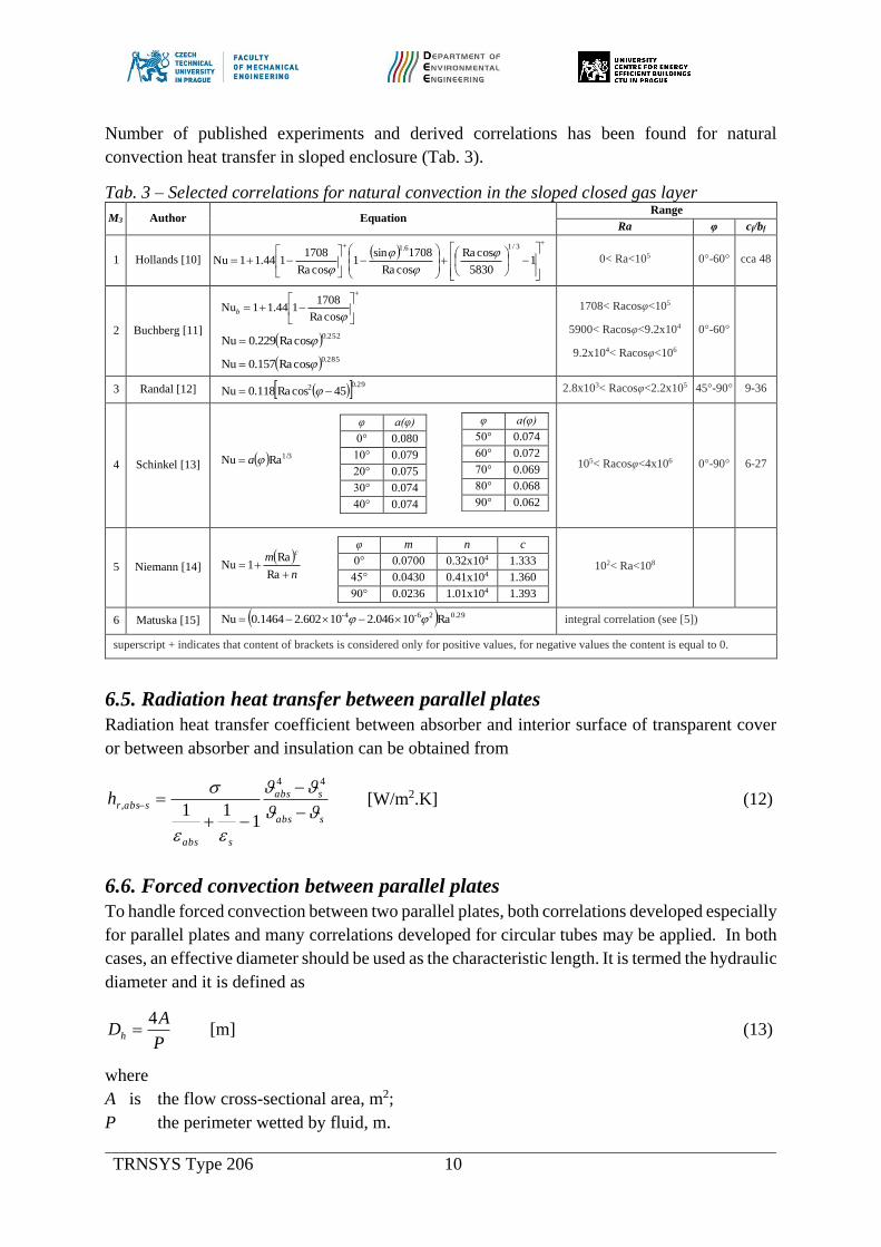
Number of published experiments and derived correlations has been found for natural

convection heat transfer in sloped enclosure (Tab. 3).

Tab. 3 – Selected correlations for natural convection in the sloped closed gas layer

M3 Author Equation Range

Ra φ cf/bf

1 Hollands [10]

1

5830

cosRa

cosRa

1708sin1

cosRa

1708144.11Nu

3/16.1

0< Ra<105 0°-60° cca 48

2 Buchberg [11]

cosRa

1708144.11Nub

252.0cosRa229.0Nu

285.0cosRa157.0Nu

1708< Racosφ<105

5900< Racosφ<9.2x104

9.2x104< Racosφ<106

0°-60°

3 Randal [12] 29.02 45cosRa118.0Nu 2.8x103< Racosφ<2.2x105 45°-90° 9-36

4 Schinkel [13]

1/3RaNu a

φ a(φ)

0° 0.080

10° 0.079

20° 0.075

30° 0.074

40° 0.074

φ a(φ)

50° 0.074

60° 0.072

70° 0.069

80° 0.068

90° 0.062

105< Racosφ<4x106 0°-90° 6-27

5 Niemann [14]

n

mc

Ra

Ra1Nu

φ m n c

0° 0.0700 0.32x104 1.333

45° 0.0430 0.41x104 1.360

90° 0.0236 1.01x104 1.393

102< Ra<108

6 Matuska [15] 0.292-6-4 Ra102.046102.6020.1464Nu integral correlation (see [5])

superscript + indicates that content of brackets is considered only for positive values, for negative values the content is equal to 0.

6.5. Radiation heat transfer between parallel plates

Radiation heat transfer coefficient between absorber and interior surface of transparent cover

or between absorber and insulation can be obtained from

sabs

sabs

sabs

sabsrh

44

,

111

[W/m2.K] (12)

6.6. Forced convection between parallel plates

To handle forced convection between two parallel plates, both correlations developed especially

for parallel plates and many correlations developed for circular tubes may be applied. In both

cases, an effective diameter should be used as the characteristic length. It is termed the hydraulic

diameter and it is defined as

P

ADh

4 [m] (13)

where

A is the flow cross-sectional area, m2;

P the perimeter wetted by fluid, m.

TRNSYS Type 206 11

Then forced convection heat transfer coefficient is determined from Nusselt number

h

f

DcD

h

Nu [W/m2.K] (14)

where

λf is thermal conductivity of heat transfer fluid, W/m.K;

In the presented Type 206, the coefficients for both upper and lower surfaces of each channel

are assumed equal, hc1 = hc2 and hc3 = hc4.

6.6.1. Turbulent flow region (Re > 10000)

Turbulent forced convection heat transfer is widely described. Tab. 4 shows correlations for

Nusselt number for turbulent forced convection heat transfer found in the literature.

Tab. 4 – Selected correlations for turbulent flow region

M4 Author Equation Comment

1

Kays and

Crawford

[16]

8.0Re0158.0Nu DD developed for solar air

collectors, Re > 3000

2 Tan and

Charters [17] 4.08.0 PrRe018.0Nu DD

developed for solar air

collectors,

9500 < Re < 22000

3 Nusselt [18] 055.0318.0 PrRe036.0Nu LDhDD

developed for circular

tube,

10 < L/D < 400

4 Sieder and Tate

[19] 14.0318.0 PrRe027.0Nu wDD

developed for circular

tube,

Re > 10000

5 Dittus-

Boelter [20] coolingfor PrRe0265.0Nu

heatingfor PrRe0243.0Nu

3.054

4.054

DD

DD

developed for circular

tube,

Re > 10000

6 Gnielinski

[21]

2

10

3/221

64.1Relog82.1 pipes smoth

diagram Moody´s toaccordingfactor friction

1Pr87.121

Pr1000Re8Nu

D

DD

f

f

f

developed for circular

tube, more accurate,

3000 < Re < 5 x 106

7 Petukhov [22]

2

10

3/221

64.1Relog82.1 pipes smoth

diagram Moody´s toaccordingfactor friction

1Pr87.121

PrRe8Nu

D

DD

f

f

f

circular tube, more

accurate,

3000 < Re < 5 x 106

TRNSYS Type 206 12

6.6.1. Transition flow region (2300 < Re < 6000)

Hausen [23] presented the following empirical correlation for the average Nusselt number

beginning of the heated section and the position L for flow in a tube:

14.0323132 1Pr125Re116.0Nu whDD LD [-] (15)

6.6.2. Laminar flow region (Re < 2300)

For laminar flow, the use of circular tube correlations is less accurate, particularly for cross

sections characterized by sharp corners. For such cases the Nusselt number corresponding to

fully developed conditions may be obtained from the following empirical correlation developed

for laminar flow between two parallel flat plates with one side insulated and the other subjected

to a constant heat flux [24]:

17.1

71.1

PrRe00563.01

PrRe0019.04.5Nu

LD

LD

h

hD

[-] (16)

6.7. Radiation heat exchange between frame and adjacent ambient surfaces

Radiation heat transfer coefficient between exterior surface of collector back frame and adjacent

surfaces in ambient environment (roof) related to ambient temperature ϑamb can be expressed as

ambb

ambb

asb

ambbrh

2

44

2

2

2,

111

[W/m2.K] (17)

6.2. Reverse temperature calculation

6.2.1. Mode 1

In steady state, the performance of a solar collector is described by an energy balance that

indicates the distribution of incident solar energy into useful energy gain, thermal losses, and

optical losses. The solar radiation absorbed by a collector per unit area of absorber Aabs is equal

to the difference between the incident solar radiation and the optical. The thermal energy lost

from the collector to the surroundings by conduction, convection, and infrared radiation can be

represented as the product of heat transfer coefficient U, times the difference between the mean

fluid temperature ϑfluid and the ambient temperature ϑamb:

ambfluidtabsnabsu UGFAQ [W] (18)

The problem with this equation is that the overall heat loss coefficient U and the collector

efficiency factor F΄ is difficult to calculate. The algebra is somewhat tedious and only results

of deriving F΄ and U are presented in Fig. 5. More information about F΄ and U deriving can be

found in Duffie and Beckman [25].

TRNSYS Type 206 13

212,222,1

2122,12,21

ccfabsrctcfabsrc

cctbcfabsrcfabsrcctb

hhhhUhhh

hhUUhhhhhhUUU

[W/m2.K] (19)

2

2,2,212,

212,2212,

fabsrfabsrcbcfabsrt

ccfabsrctccfabsr

hhhUhhU

hhhhUhhhF

[-] (20)

bt UUU [W/m2.K] (21)

2,2

1 11

11

1

babsrc

c

hh

h

UF

[-] (22)

TRNSYS Type 206 14

Fig. 5 – Overall heat loss coefficients and efficiency factors for different solar air collector

designs (Design 3 and 4 not available yet)

After that the collector flow factor F΄΄ and the collector heat removal factor FR can be obtained

as follows

Fcm

UA

FUA

cmF

f

abs

abs

f

exp1 [-] (23)

where

cf is specific thermal capacity of fluid, J/kg.K;

m total mass flow rate of fluid through air channel, kg/s,

FFFR [-] (24)

Then the useful energy gain is determined

ambintabsnRabsu UGFAQ [W] (25)

and the outlet temperature

f

uinout

cm

Q

[K] (26)

Since the useful heat energy gain, the collector heat removal factor and the collector efficiency

factor have been calculated for first estimates of temperatures, next iteration step should follow.

To calculate heat transfer coefficients at main surfaces of solar collector and to assess the overall

collector heat loss coefficient U in the next iteration step the absorber temperature, the mean

fluid temperature, and the temperature distribution should be derived

R

absR

uinabs F

UAF

Q 1

[K] (27)

FUAF

Q

absR

uinfluid

1

[K] (28)

ncfabsr

ambabstncfabsrabs

fhh

Uhh

2,

2,

2

[K] (29)

TRNSYS Type 206 15

21,

21,2

1

ffcd

ambabstffcdf

fh

Uh

[K] (30)

bbabsrc

ambbbabsrabscfluid

bUhh

Uhh

2,2

2,2

2

[K] (31)

21,

221,2

1

bbcd

ambbbbbcdb

bh

Uh

[K] (32)

6.2 Mode 2

Mode 2 operates in a principally different manner. The core of the Mode 2 is a set of heat

balance equations obtained from the thermal network at the points:

1221,11,11,1 : ffffcdambfambfwskyfambfrf hhh (33)

222,1221,2 : fabsncfabsfabsrffffcdf hhh (34)

fluidabscbabsbabsrfabsncfabsrnetabs hhhhGK 122,22,: (35)

influid

f

bfluidcfluidabscfluidac

mchh

2: 221 (36)

1221,2222,2 : bbbbcdbfluidcbabsbabsrb hhh (37)

ambbambbwambbambbrbbbbcdb hhh 21,22,1221,1 : (38)

By rearranging, we obtain a system of linear equations in the matrix form:

(39)

ambambbwambambbr

in

f

net

ambambfwskyambfr

b

b

fluid

abs

f

f

bbcdambbwambbrbbcd

bbcdbbcdcbabsr

c

babsr

hh

ac

mc

GK

hh

hhhh

hhhh

h

h

1,1,

1,1,

1

2

2

1

21,1,1,21,

21,21,22,

2

2,

0

2

0

0

0

00

00

In general, the above matrices may be displayed as

BTA (40)

0

2

0

0

000

00

00

0

0

2

21

1

2,

1

12,2,2,

2,2,21,21,

21,21,1,1,

c

f

cc

c

babsr

c

cbabsrncfabsrncfabsr

ncfabsrncfabsrffcdffcd

ffcdffcdambfwambfr

hac

mchh

h

h

h

hhhhhh

hhhhhh

hhhh

TRNSYS Type 206 16

The mean temperature vector may be determined by matrix inversion as

BAT1

(41)

Then the outlet fluid temperature and the useful energy gain can be determined

influidout 2 [K] (42)

influidfu mcQ [W] (43)

6.3. Iterative procedure

The newly-calculated temperatures values ϑout, ϑabs, and ϑfluid are then compared with previously

assumed ones. The iterative process is repeated until all consecutive outlet temperatures,

absorber temperatures, and heat transfer fluid temperatures differ by less than 0.01 K. Normally,

the number of iterations required is not more than four or five.

6.4. Instantaneous efficiency

Finally, the instantaneous solar air collector efficiency is

tG

u

GA

Q [-] (44)

where

Gt is total radiation for collector surface, W/m2;

netgndskybeamt KGGGG [W/m2] (45)

where

Knet is net incident angle modifier.

6.5. Incident angle modifier Knet

The collector absorbs only a portion of the solar irradiance due to the optical properties of the

transparent cover and absorber plate, which are described in the τnαabs and the IAM parameters

for each irradiance component (Kbeam, Ksky, Kgnd). Incident angle modifiers are calculated

separately for beam (Gbeam), sky (Gsky) and ground radiation (Ggnd). The net incident angle

modifier for all incident radiation is calculated by weighting each component by the

corresponding modifier.

t

gndgndskyskybeambeamnet

G

KGKGKGK

[-] (46)

Incidence angle modifier of solar collector for beam radiation component can be determined by

experiment:

2

10 1cos

11

cos

11

bbKbeam [-] (47)

TRNSYS Type 206 17

Sky and ground reflected radiation are considered as diffuse isotropic, that means optical

properties for this solar radiation components are not considered as incidence angle dependent

like for beam radiation but constant. Incidence angle modifier of solar collector for sky and

ground radiation components can be approximated using Brandemuehl and Beckman’s

equations [29] from the Kbeam characteristic for given effective incident angle:

2, 001497.01388.068.59 skyeff [°] (48)

2, 002693.05788.090 gndeff [°] (49)

Finally incident angle modifiers for sky-diffuse and ground-reflected radiation are:

2

,

1

,

0 1cos

11

cos

11

skyeffskyeff

sky bbK

[-] (50)

2

,

1

,

0 1cos

11

cos

11

gndeffgndeff

gnd bbK

[-] (51)

In the case of b1 = 0, incident angle modifiers for beam, sky and ground radiation have to be

calculated by another equations:

30

60,60max11

cos,5.0max

11 0

0

bbKbeam [-] (52)

30

60,60max11

cos,5.0max

11

,0

,

0

skyeff

skyeff

sky

bbK

[-] (53)

30

60,60max11

cos,5.0max

11

,0

,

0

gndeff

gndeff

gnd

bbK

[-] (54)

7. Experimental validation (to be added in 2018)

8. References [1] Hottel H, Woertz B. Performance of flat-plate solar-heat collectors. Trans ASME (Am

Soc Mech Eng); (United States) 1942;64:91–104.

[2] Hottel H, Whillier A. Evaluation of flat-plate solar collector performance. Trans Conf

Use Sol Energy; 1955;3:74–104.

[3] Bliss Jr. RW. The derivations of several “Plate-efficiency factors” useful in the design

of flat-plate solar heat collectors. Sol Energy 1959;3:55–64. doi:10.1016/0038-

092X(59)90006-4.

[4] Smith CC, Weiss TA. Design application of the Hottel-Whillier-Bliss equation. Sol

Energy 1977;19:109–13. doi:10.1016/0038-092X(77)90047-0.

TRNSYS Type 206 18

[5] Mcadams WH. Heat Transmission 3d Ed. New York: McGraw-Hill; 1954.

[6] J. H. DW, W. W. S. C, Proctor. Solar and wind induced external coefficients for solar

collectors. Coop Mediterr Pour l’Energie Solaire, Rev Int d’Heliotechnique 1977;2:56.

[7] Test FL, Lessmann RC. An Experimental Study of Heat Transfer During Forced

Convection over a Rectangular Body. J Heat Transfer 1980;102:146–51.

[8] Test FL, Lessmann RC, Johary A. Heat Transfer During Wind Flow over Rectangular

Bodies in the Natural Environment. J Heat Transfer 1981;103:262–7.

[9] Kumar S, Sharma VB, Kandpal TC, Mullick SC. Wind induced heat losses from outer

cover of solar collectors. Renew Energy 1997;10:613–6. doi:10.1016/S0960-

1481(96)00031-6.

[10] Hollands KGT, Unny TE, Raithby GD, Konicek L. Free Convective Heat Transfer

Across Inclined Air Layers. J Heat Transfer 1976;98:189–93.

[11] Buchberg H, Catton I, Edwards DK. Natural Convection in Enclosed Spaces - A

Review of Application to Solar Energy Collection. J Heat Transfer 1976;98:182–8.

[12] Randall KR, Mitchell JW, El-Wakil MM. Natural Convection Heat Transfer

Characteristics of Flat Plate Enclosures. J Heat Transfer 1979;101:120–5.

[13] Schinkel W. Natural concection in inclined air-filled enclosures. Delft: Dutch

Efficiency Bureau - Pijnacker; 1980.

[14] Niemann H. Die Wärmeübertragung durch natürliche Konvektion in spaltförmigen

Hohlräumen. Gesund Ing 1948;69:224–8.

[15] Matuska T, Zmrhal V. A mathematical model and design tool KOLEKTOR 2.2

reference handbook. Prague: 2009.

[16] Kays WM, Crawford ME. Convective Heat and Mass Transfer, 2nd edn McGraw-Hill.

New York 1980:141.

[17] Tan HM, Charters WWS. Effect of thermal entrance region on turbulent forced-

convective heat transfer for an asymmetrically heated rectangular duct with uniform

heat flux. Sol Energy 1969;12:513–6. doi:10.1016/0038-092X(69)90072-3.

[18] Nusselt W. Der Wärmeaustausch zwischen Wand und Wasser im Rohr. Forsch Auf

Dem Gebiete Des Ingenieurwesens 1931;2:309–13. doi:10.1007/BF02583210.

[19] Sieder EN, Tate GE. Heat Transfer and Pressure Drop of Liquids in Tubes. Ind Eng

Chem 1936;28:1429–35. doi:10.1021/ie50324a027.

[20] Dittus FW, Boelter LMK. Heat transfer in automobile radiators of the tubular type. Int

Commun Heat Mass Transf 1985;12:3–22.

[21] Gnielinski V. New equations for heat and mass transfer in turbulent pipe and channel

flow. Int Chem Eng 1976;16:359–68.

[22] Petukhov BS. Heat transfer and friction in turbulent pipe flow with variable physical

properties. Adv Heat Transf 1970;6:503–64.

[23] Hausen H. Darstellung des Warmeuberganges in Rohren durch verallgemeinerte

TRNSYS Type 206 19

Potenzbeziehungen. Z VDI Beih Verfahrenstech 1943;4:91–8.

[24] Heaton HS, Reynolds WC, Kays WM. Heat transfer in annular passages. Simultaneous

development of velocity and temperature fields in laminar flow. Int J Heat Mass Transf

1964;7:763–81. doi:10.1016/0017-9310(64)90006-7.

[25] Duffie JA, Beckman WA. Solar engineering of thermal processes. John Wiley & Sons;

2013.

Appendix 1: Installation The Type206 solar air collector model is a TRNSYS 17 drop-in dll component. For a complete

set of files one should have:

Type206.dll – the drop-in dll file

Type206.cpp – the C++ source code

Type206.tmf – the Simulation Studio proforma

Type206.bmp – the Simulation Studio proforma icon

For installation:

1. Copy the .dll file to \TRNSYS16\UserLib\ReleaseDLLs\

2. Copy the .tmf and .bmp files to the \Proformas folder, e.g.

C:\Trnsys17\Studio\Proformas\Nonstandard\

3. Restart simulation studio if it was running.