Title of Projects: - Implementing a simple Recommender System on user based rating and testing the same.

Command for Check all Available Packages with their DataSet:-

> data(package = .packages(all.available = TRUE))

Production ready recommender engines

E-commerce websites (or for that fact, any popular technology platform) out there today have tonnes of content to offer. Not only that, but the number of users is also huge. In such a scenario, where thousands of users are browsing/buying stuff simultaneously across the globe, providing recommendations to them is a task in itself. To complicate things even further, a good user experience (response times, for example) can create a big difference between two competitors. These are live examples of production systems handling millions of customers day in and day out.

Fun Fact

Amazon.com is one of the biggest names in the e-commerce space with 244 million active customers. Imagine the amount of data being processed to provide recommendations to such a huge customer base browsing through millions of products!

Source: http://www.amazon.com/b?ie=UTF8&node=8445211011

In order to provide a seamless capability for use in such platforms, we need highly optimized libraries and hardware. For a recommender engine to handle thousands of users simultaneously every second, R has a robust and reliable framework called the recommenderlab.

Recommenderlab is a widely used R extension designed to provide a robust foundation for recommender engines. The focus of this library is to provide efficient handling of data, availability of standard algorithms and evaluation capabilities. In this section, we will be using recommenderlab to handle a considerably large data set for recommending items to users. We will also use the evaluation functions from recommenderlab to see how good or bad our recommendation system is. These capabilities will help us build a production ready recommender system similar (or at least closer) to what many online applications such as Amazon or Netflix use.

The dataset used in this section contains ratings for 100 items as rated by 5000 users. The data has been anonymised and the product names have been replaced by product IDs. The rating scale used is 0 to 5 with 1 being the worst, 5 being the best, and 0 representing unrated items or missing ratings.

To build a recommender engine using recommenderlab for a production ready system, the following steps are to be performed:

1. How to manage data in recommender lab and then we create and evaluate recommenders. First, we load the package

> library("recommenderlab") Error in library("recommenderlab") : there is no package called ‘recommenderlab’ > install.packages("recommenderlab") also installing the dependency ‘irlba’ trying URL 'https://cran.rstudio.com/bin/windows/contrib/3.4/irlba_2.2.1.zip' Content type 'application/zip' length 263501 bytes (257 KB) downloaded 257 KB trying URL 'https://cran.rstudio.com/bin/windows/contrib/3.4/recommenderlab_0.2-2.zip' Content type 'application/zip' length 1428312 bytes (1.4 MB) downloaded 1.4 MB package ‘irlba’ successfully unpacked and MD5 sums checked package ‘recommenderlab’ successfully unpacked and MD5 sums checked The downloaded binary packages are in C:\Users\admin\AppData\Local\Temp\Rtmpa4sOUx\downloaded_packages > m <- matrix(sample(c(as.numeric(0:5), NA), 50, + replace=TRUE, prob=c(rep(.4/6,6),.6)), ncol=10, + dimnames=list(user=paste("u",1:5,sep = ''), + item=paste("i", 1:10, sep=''))) > m item user i1 i2 i3 i4 i5 i6 i7 i8 i9 i10 u1 NA NA NA NA NA NA NA 4 5 5 u2 3 NA 0 2 NA 5 3 NA 1 NA u3 2 NA NA NA NA NA NA 5 2 NA u4 NA 4 4 NA 3 4 NA NA 5 5 u5 NA NA NA NA NA NA 4 NA 0 NA

we create a small artificial data set as a matrix.

With coercion, the matrix can be easily converted into a realRatingMatrix object which stores the data in sparse format (only non-NA values are stored explicitly; NA values are represented by a dot).

> r <- as(m, "realRatingMatrix") > r 5 x 10 rating matrix of class ‘realRatingMatrix’ with 20 ratings. > getRatingMatrix(r) 5 x 10 sparse Matrix of class "dgCMatrix" [[ suppressing 10 column names ‘i1’, ‘i2’, ‘i3’ ... ]]

u1 . . . . . . . 4 5 5 u2 3 . 0 2 . 5 3 . 1 . u3 2 . . . . . . 5 2 . u4 . 4 4 . 3 4 . . 5 5 u5 . . . . . . 4 . 0 .

The realRatingMatrix can be coerced back into a matrix which is identical to the original matrix.

> identical(as(r, "matrix"),m) [1] TRUE It can also be coerced into a list of users with their ratings for closer inspection or into a data.frame with user/item/rating tuples. > as(r, "list") $u1 i8 i9 i10 4 5 5 $u2 i1 i3 i4 i6 i7 i9 3 0 2 5 3 1 $u3 i1 i8 i9 2 5 2 $u4 i2 i3 i5 i6 i9 i10 4 4 3 4 5 5 $u5 i7 i9 4 0 > head(as(r, "data.frame")) user item rating 12 u1 i8 4 14 u1 i9 5 19 u1 i10 5 1 u2 i1 3 4 u2 i3 0 6 u2 i4 2 The data.frame version is especially suited for writing rating data to a file (e.g., by write.csv()). Coercion from data.frame (user/item/rating tuples) and list into a sparse rating matrix is also provided. This way, external rating data can easily be imported into recommenderlab.

2. Normalization An important operation for rating matrices is to normalize the entries to, e.g., centering to remove rating bias by subtracting the row mean from all ratings in the row. This is can be easily done using normalize(). R> r_m <- normalize(r) R> r_m 5 x 10 rating matrix of class ‘realRatingMatrix’ with 19 ratings. Normalized using center on rows. > r_m <- normalize(r) > r_m 5 x 10 rating matrix of class ‘realRatingMatrix’ with 20 ratings. Normalized using center on rows. > getRatingMatrix(r_m) 5 x 10 sparse Matrix of class "dgCMatrix" [[ suppressing 10 column names ‘i1’, ‘i2’, ‘i3’ ... ]] u1 . . . . . . . -0.6666667 0.3333333 u2 0.6666667 . -2.3333333 -0.3333333 . 2.6666667 0.6666667 . -1.3333333 u3 -1.0000000 . . . . . . 2.0000000 -1.0000000 u4 . -0.1666667 -0.1666667 . -1.166667 -0.1666667 . . 0.8333333 u5 . . . . . . 2.0000000 . -2.0000000 u1 0.3333333 u2 . u3 . u4 0.8333333 u5 . Normalization can be reversed using denormalize(). > denormalize(r_m) 5 x 10 rating matrix of class ‘realRatingMatrix’ with 20 ratings.

3. Binarization

Binarization of data A matrix with real valued ratings can be transformed into a 0-1 matrix with binarize() and a user specified threshold (min_ratings) on the raw or normalized ratings. In the following only items with a rating of 4 or higher will become a positive rating in the new binary rating matrix.

> r_b <- binarize(r, minRating=4) > r_b 5 x 10 rating matrix of class ‘binaryRatingMatrix’ with 11 ratings. > as(r_b, "matrix") i1 i2 i3 i4 i5 i6 i7 i8 i9 i10 u1 FALSE FALSE FALSE FALSE FALSE FALSE FALSE TRUE TRUE TRUE u2 FALSE FALSE FALSE FALSE FALSE TRUE FALSE FALSE FALSE FALSE u3 FALSE FALSE FALSE FALSE FALSE FALSE FALSE TRUE FALSE FALSE u4 FALSE TRUE TRUE FALSE FALSE TRUE FALSE FALSE TRUE TRUE u5 FALSE FALSE FALSE FALSE FALSE FALSE TRUE FALSE FALSE FALSE

4. Inspection of data set properties

We will use the data set Jester5k for the rest of this section. This data set comes with recommenderlab and contains a sample of 5000 users from the anonymous ratings data from the Jester Online Joke Recommender System collected between April 1999 and May 2003 (Goldberg, Roeder, Gupta, and Perkins 2001). The data set contains ratings for 100 jokes on a scale from −10 to +10. All users in the data set have rated 36 or more jokes.

> data(Jester5k) > Jester5k 5000 x 100 rating matrix of class ‘realRatingMatrix’ with 362106 ratings.

Jester5k contains 362106 ratings. For the following examples we use only a subset of the data containing a sample of 1000 users (we set the random number generator seed for reproducibility). For random sampling sample() is provided for rating matrices.

> set.seed(1234) > r <- sample(Jester5k, 1000) > r 1000 x 100 rating matrix of class ‘realRatingMatrix’ with 71682 ratings.

This subset still contains 71682 ratings. Next, we inspect the ratings for the first user. We can select an individual user with the extraction operator.

> rowCounts(r[1,]) u5092 70 > as(r[1,], "list") $u5092 j1 j2 j3 j4 j5 j6 j7 j8 j9 j10 j11 j12 j13 -3.40 -3.40 -1.99 1.31 -4.03 -0.15 -4.22 -4.56 -4.37 -0.34 0.53 -5.87 -2.57

j14 j15 j16 j17 j18 j19 j20 j21 j22 j23 j24 j25 j26 -5.39 0.44 -3.98 -3.35 -4.03 -4.03 -0.29 -3.79 -3.59 0.05 -6.94 -0.53 -2.57 j27 j28 j29 j30 j31 j32 j33 j34 j35 j36 j37 j38 j39 1.80 -5.87 2.14 -4.42 -1.70 0.68 -7.82 -0.49 -0.92 2.38 -7.96 -5.15 -5.87 j40 j41 j42 j43 j44 j45 j46 j47 j48 j49 j50 j51 j52 -7.23 -4.37 -2.33 -5.15 0.34 3.40 -1.60 -2.04 -3.11 2.82 2.96 -3.35 1.07 j53 j54 j55 j56 j57 j58 j59 j60 j61 j62 j63 j64 j65 0.10 -6.99 0.78 -2.57 -6.75 -6.60 -4.51 1.46 -1.55 1.12 -7.48 -7.96 2.52 j66 j67 j68 j69 j70 0.49 -3.25 -1.21 2.18 -5.87 > rowMeans(r[1,]) u5092 -2.413429

The user has rated 70 jokes, the list shows the ratings and the user’s rating average is - 2.41342857142857 . Next, we look at several distributions to understand the data better. getRatings() extracts a vector with all non-missing ratings from a rating matrix.

> hist(getRatings(r), breaks=100)

In the histogram in Figure 5 shoes an interesting distribution where all negative values occur with a almost identical frequency and the positive ratings more frequent with a steady decline

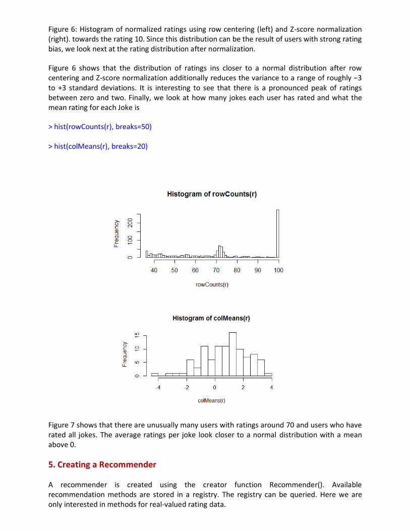
Figure 6: Histogram of normalized ratings using row centering (left) and Z-score normalization (right). towards the rating 10. Since this distribution can be the result of users with strong rating bias, we look next at the rating distribution after normalization.

Figure 6 shows that the distribution of ratings ins closer to a normal distribution after row centering and Z-score normalization additionally reduces the variance to a range of roughly −3 to +3 standard deviations. It is interesting to see that there is a pronounced peak of ratings between zero and two. Finally, we look at how many jokes each user has rated and what the mean rating for each Joke is

> hist(rowCounts(r), breaks=50) > hist(colMeans(r), breaks=20)

Figure 7 shows that there are unusually many users with ratings around 70 and users who have rated all jokes. The average ratings per joke look closer to a normal distribution with a mean above 0.

5. Creating a Recommender

A recommender is created using the creator function Recommender(). Available recommendation methods are stored in a registry. The registry can be queried. Here we are only interested in methods for real-valued rating data.

> recommenderRegistry$get_entries(dataType = "realRatingMatrix") $ALS_realRatingMatrix Recommender method: ALS for realRatingMatrix Description: Recommender for explicit ratings based on latent factors, calculated by alternating least squares algorithm. Reference: Yunhong Zhou, Dennis Wilkinson, Robert Schreiber, Rong Pan (2008). Large-Scale Parallel Collaborative Filtering for the Netflix Prize, 4th Int'l Conf. Algorithmic Aspects in Information and Management, LNCS 5034. Parameters: normalize lambda n_factors n_iterations min_item_nr seed 1 NULL 0.1 10 10 1 NULL $ALS_implicit_realRatingMatrix Recommender method: ALS_implicit for realRatingMatrix Description: Recommender for implicit data based on latent factors, calculated by alternating least squares algorithm. Reference: Yifan Hu, Yehuda Koren, Chris Volinsky (2008). Collaborative Filtering for Implicit Feedback Datasets, ICDM '08 Proceedings of the 2008 Eighth IEEE International Conference on Data Mining, pages 263-272. Parameters: lambda alpha n_factors n_iterations min_item_nr seed 1 0.1 10 10 10 1 NULL $IBCF_realRatingMatrix Recommender method: IBCF for realRatingMatrix Description: Recommender based on item-based collaborative filtering. Reference: NA Parameters: k method normalize normalize_sim_matrix alpha na_as_zero 1 30 "Cosine" "center" FALSE 0.5 FALSE $POPULAR_realRatingMatrix Recommender method: POPULAR for realRatingMatrix Description: Recommender based on item popularity. Reference: NA Parameters: normalize aggregationRatings aggregationPopularity 1 "center" new("standardGeneric" new("standardGeneric" $RANDOM_realRatingMatrix Recommender method: RANDOM for realRatingMatrix Description: Produce random recommendations (real ratings). Reference: NA Parameters: None $RERECOMMEND_realRatingMatrix Recommender method: RERECOMMEND for realRatingMatrix Description: Re-recommends highly rated items (real ratings). Reference: NA

Parameters: randomize minRating 1 1 NA $SVD_realRatingMatrix Recommender method: SVD for realRatingMatrix Description: Recommender based on SVD approximation with column-mean imputation. Reference: NA Parameters: k maxiter normalize 1 10 100 "center" $SVDF_realRatingMatrix Recommender method: SVDF for realRatingMatrix Description: Recommender based on Funk SVD with gradient descend. Reference: NA Parameters: k gamma lambda min_epochs max_epochs min_improvement normalize verbose 1 10 0.015 0.001 50 200 1e-06 "center" FALSE $UBCF_realRatingMatrix Recommender method: UBCF for realRatingMatrix Description: Recommender based on user-based collaborative filtering. Reference: NA Parameters: method nn sample normalize 1 "cosine" 25 FALSE "center"

Next, we create a recommender which generates recommendations solely on the popularity of items (the number of users who have the item in their profile). We create a recommender from the first 1000 users in the Jester5k data set.

> r <- Recommender(Jester5k[1:1000], method = "POPULAR") > r Recommender of type ‘POPULAR’ for ‘realRatingMatrix’ learned using 1000 users.

Recommender of type ‘POPULAR’ for ‘realRatingMatrix’ learned using 1000 users. The model can be obtained from a recommender using getModel().

> names(getModel(r)) [1] "topN" "ratings" "normalize" [4] "aggregationRatings" "aggregationPopularity" "verbose" > getModel(r)$topN Recommendations as ‘topNList’ with n = 100 for 1 users.

Recommendations as ‘topNList’ with n = 100 for 1 users. In this case the model has a top-N list to store the popularity order and further elements (average ratings, if it used normalization and

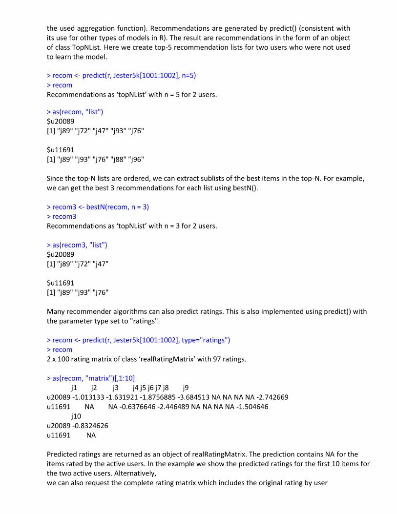
the used aggregation function). Recommendations are generated by predict() (consistent with its use for other types of models in R). The result are recommendations in the form of an object of class TopNList. Here we create top-5 recommendation lists for two users who were not used to learn the model.

> recom <- predict(r, Jester5k[1001:1002], n=5) > recom Recommendations as ‘topNList’ with n = 5 for 2 users.

> as(recom, "list") $u20089 [1] "j89" "j72" "j47" "j93" "j76" $u11691 [1] "j89" "j93" "j76" "j88" "j96" Since the top-N lists are ordered, we can extract sublists of the best items in the top-N. For example, we can get the best 3 recommendations for each list using bestN(). > recom3 <- bestN(recom, n = 3) > recom3 Recommendations as ‘topNList’ with n = 3 for 2 users. > as(recom3, "list") $u20089 [1] "j89" "j72" "j47" $u11691 [1] "j89" "j93" "j76" Many recommender algorithms can also predict ratings. This is also implemented using predict() with the parameter type set to "ratings". > recom <- predict(r, Jester5k[1001:1002], type="ratings") > recom 2 x 100 rating matrix of class ‘realRatingMatrix’ with 97 ratings. > as(recom, "matrix")[,1:10] j1 j2 j3 j4 j5 j6 j7 j8 j9 u20089 -1.013133 -1.631921 -1.8756885 -3.684513 NA NA NA NA -2.742669 u11691 NA NA -0.6376646 -2.446489 NA NA NA NA -1.504646 j10 u20089 -0.8324626 u11691 NA Predicted ratings are returned as an object of realRatingMatrix. The prediction contains NA for the items rated by the active users. In the example we show the predicted ratings for the first 10 items for the two active users. Alternatively, we can also request the complete rating matrix which includes the original rating by user

> recom <- predict(r, Jester5k[1001:1002], type="ratingMatrix") > recom 2 x 100 rating matrix of class ‘realRatingMatrix’ with 200 ratings.

> as(recom, "matrix")[,1:10] j1 j2 j3 j4 j5 j6 j7 u20089 -1.013133 -1.631921 -1.8756885 -3.684513 9.710227 2.380227 -8.499773 u11691 -2.887797 -5.797797 -0.6376646 -2.446489 -5.027797 4.972203 -8.327797 j8 j9 j10 u20089 9.850227 -2.742669 -0.8324626 u11691 2.162203 -1.504646 -4.1977966

6. Evaluation of predicted ratings

Next, we will look at the evaluation of recommender algorithms. recommenderlab implements several standard evaluation methods for recommender systems. Evaluation starts with creating an evaluation scheme that determines what and how data is used for training and testing. Here we create an evaluation scheme which splits the first 1000 users in Jester5k into a training set (90%) and a test set (10%). For the test set 15 items will be given to the recommender algorithm and the other items will be held out for computing the error. > e <- evaluationScheme(Jester5k[1:1000], method="split", train=0.9, + given=15, goodRating=5) > e Evaluation scheme with 15 items given Method: ‘split’ with 1 run(s). Training set proportion: 0.900 Good ratings: >=5.000000 Data set: 1000 x 100 rating matrix of class ‘realRatingMatrix’ with 72358 ratings We create two recommenders (user-based and item-based collaborative filtering) using the training data.

> r1 <- Recommender(getData(e, "train"), "UBCF") > r1 Recommender of type ‘UBCF’ for ‘realRatingMatrix’ learned using 900 users.

> r2 <- Recommender(getData(e, "train"), "IBCF") > r2 Recommender of type ‘IBCF’ for ‘realRatingMatrix’ learned using 900 users.

> p1 <- predict(r1, getData(e, "known"), type="ratings") > p1 100 x 100 rating matrix of class ‘realRatingMatrix’ with 8500 ratings.

> p2 <- predict(r2, getData(e, "known"), type="ratings") > p2 100 x 100 rating matrix of class ‘realRatingMatrix’ with 8445 ratings.

Finally, we can calculate the error between the prediction and the unknown part of the test data. > error <- rbind( + UBCF = calcPredictionAccuracy(p1, getData(e, "unknown")), + IBCF = calcPredictionAccuracy(p2, getData(e, "unknown"))

+ ) > error RMSE MSE MAE UBCF 4.353456 18.95258 3.413487 IBCF 4.975929 24.75987 3.894817

In this example user-based collaborative filtering produces a smaller prediction error. 7. Evaluation of a top-N recommender algorithm For this example we create a 4-fold cross validation scheme with the the Given-3 protocol, i.e., for the test users all but three randomly selected items are withheld for evaluation. > scheme <- evaluationScheme(Jester5k[1:1000], method="cross", k=4, given=3, + goodRating=5) > scheme Evaluation scheme with 3 items given Method: ‘cross-validation’ with 4 run(s). Good ratings: >=5.000000 Data set: 1000 x 100 rating matrix of class ‘realRatingMatrix’ with 72358 ratings.

Next we use the created evaluation scheme to evaluate the recommender method popular. We evaluate top-1, top-3, top-5, top-10, top-15 and top-20 recommendation lists. > results <- evaluate(scheme, method="POPULAR", type = "topNList", + n=c(1,3,5,10,15,20)) POPULAR run fold/sample [model time/prediction time] 1 [0.08sec/0.63sec] 2 [0.02sec/0.61sec] 3 [0.02sec/0.7sec] 4 [0.01sec/0.63sec] > results Evaluation results for 4 folds/samples using method ‘POPULAR’. The result is an object of class EvaluationResult which contains several confusion matrices. getConfusionMatrix() will return the confusion matrices for the 4 runs (we used 4-fold cross evaluation) as a list. In the following we look at the first element of the list which represents the first of the 4 runs. > getConfusionMatrix(results)[[1]] TP FP FN TN precision recall TPR FPR 1 0.488 0.512 16.016 79.984 0.4880 0.04038575 0.04038575 0.006030783 3 1.296 1.704 15.208 78.792 0.4320 0.11019655 0.11019655 0.020377245 5 2.084 2.916 14.420 77.580 0.4168 0.16708598 0.16708598 0.034883361 10 4.052 5.948 12.452 74.548 0.4052 0.31214877 0.31214877 0.070909131 15 5.736 9.264 10.768 71.232 0.3824 0.41957216 0.41957216 0.110525891 20 7.128 12.872 9.376 67.624 0.3564 0.50118749 0.50118749 0.154023324

For the first run we have 6 confusion matrices represented by rows, one for each of the six different top-N lists we used for evaluation. n is the number of recommendations per list. TP, FP, FN and TN are the entries for true positives, false positives, false negatives and true negatives in the confusion matrix. The remaining columns contain precomputed performance measures. The average for all runs can be obtained from the evaluation results directly using avg(). > avg(results) TP FP FN TN precision recall TPR FPR 1 0.451 0.549 16.720 79.280 0.4510 0.03702692 0.03702692 0.006504849 3 1.254 1.746 15.917 78.083 0.4180 0.09574697 0.09574697 0.020981728 5 2.032 2.968 15.139 76.861 0.4064 0.14672405 0.14672405 0.035638995 10 3.926 6.074 13.245 73.755 0.3926 0.28081508 0.28081508 0.073154805 15 5.649 9.351 11.522 70.478 0.3766 0.39294814 0.39294814 0.112698641 20 7.042 12.958 10.129 66.871 0.3521 0.47678138 0.47678138 0.156597293

Evaluation results can be plotted using plot(). The default plot is the ROC curve

which plots the true positive rate (TPR) against the false positive rate (FPR).

> plot(results, annotate=TRUE)

> plot(results, "prec/rec", annotate=TRUE)

8. Comparing recommender algorithms

Comparing top-N recommendations The comparison of several recommender algorithms is one of the main functions of recommenderlab. For comparison also evaluate() is used. The only change is to use evaluate() with a list of algorithms together with their parameters instead of a single method name. In the following we use the evaluation scheme created above to compare the five recommender algorithms: random items, popular items, user-based CF, item-based CF, and SVD approximation. Note that when running the following code, the CF based algorithms are very slow. For the evaluation we use a “all-but-5” scheme. This is indicated by a negative number for given. > scheme <- evaluationScheme(Jester5k[1:1000], method="split", train = .9, + k=1, given=-5, goodRating=5) > scheme Evaluation scheme using all-but-5 items Method: ‘split’ with 1 run(s). Training set proportion: 0.900 Good ratings: >=5.000000 Data set: 1000 x 100 rating matrix of class ‘realRatingMatrix’ with 72358 ratings. > algorithms <- list( + "random items" = list(name="RANDOM", param=NULL), + "popular items" = list(name="POPULAR", param=NULL), + "user-based CF" = list(name="UBCF", param=list(nn=50)), + "item-based CF" = list(name="IBCF", param=list(k=50)), + "SVD approximation" = list(name="SVD", param=list(k = 50)) + ) > results <- evaluate(scheme, algorithms, type = "topNList", +

+ n=c(1, 3, 5, 10, 15, 20)) RANDOM run fold/sample [model time/prediction time] 1 [0sec/0.06sec] POPULAR run fold/sample [model time/prediction time] 1 [0.04sec/0.32sec] UBCF run fold/sample [model time/prediction time] 1 [0.06sec/0.69sec] IBCF run fold/sample [model time/prediction time] 1 [0.17sec/0.04sec] SVD run fold/sample [model time/prediction time] 1 Warning in irlba::irlba(m, nv = p$k, maxit = p$maxiter) : You're computing too large a percentage of total singular values, use a standard svd instead. [0.22sec/0.04sec] The result is an object of class evaluationResultList for the five

recommender algorithms.

> results List of evaluation results for 5 recommenders: Evaluation results for 1 folds/samples using method ‘RANDOM’. Evaluation results for 1 folds/samples using method ‘POPULAR’. Evaluation results for 1 folds/samples using method ‘UBCF’. Evaluation results for 1 folds/samples using method ‘IBCF’. Evaluation results for 1 folds/samples using method ‘SVD’.

Individual results can be accessed by list subsetting using an index or the name

specified when calling evaluate().

> names(results) [1] "random items" "popular items" "user-based CF" [4] "item-based CF" "SVD approximation" > results[["user-based CF"]] Evaluation results for 1 folds/samples using method ‘UBCF’.

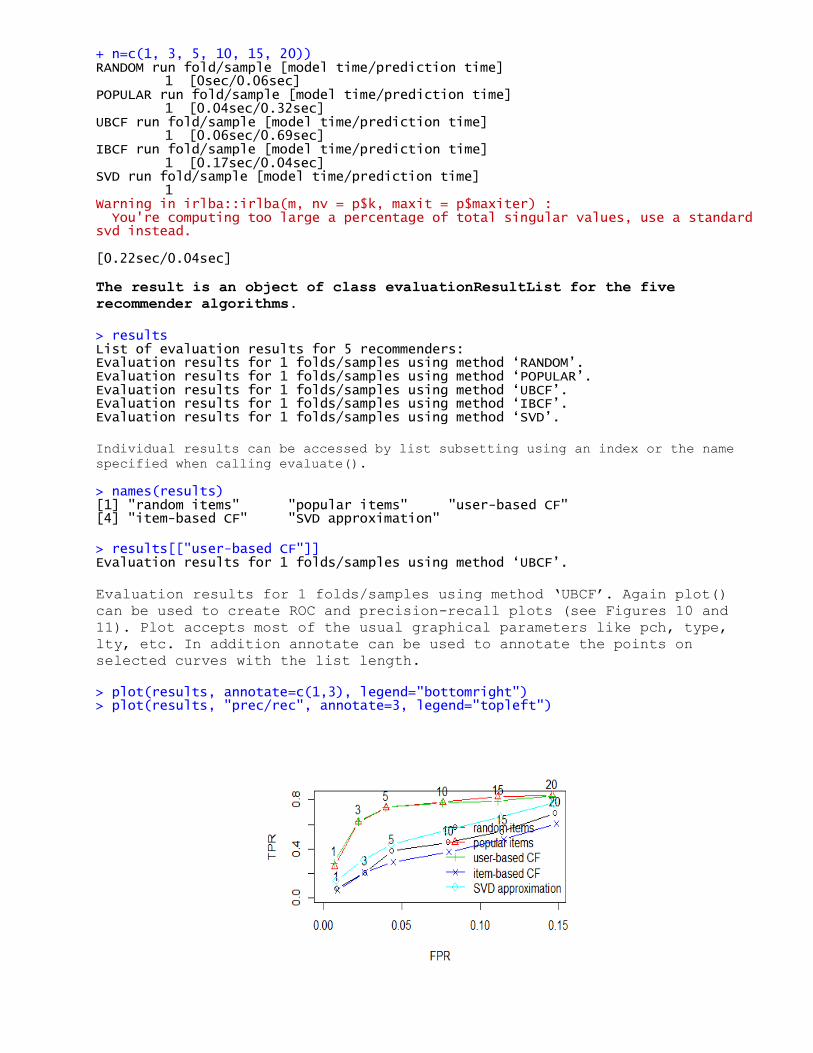
Evaluation results for 1 folds/samples using method ‘UBCF’. Again plot()

can be used to create ROC and precision-recall plots (see Figures 10 and

11). Plot accepts most of the usual graphical parameters like pch, type,

lty, etc. In addition annotate can be used to annotate the points on

selected curves with the list length.

> plot(results, annotate=c(1,3), legend="bottomright") > plot(results, "prec/rec", annotate=3, legend="topleft")

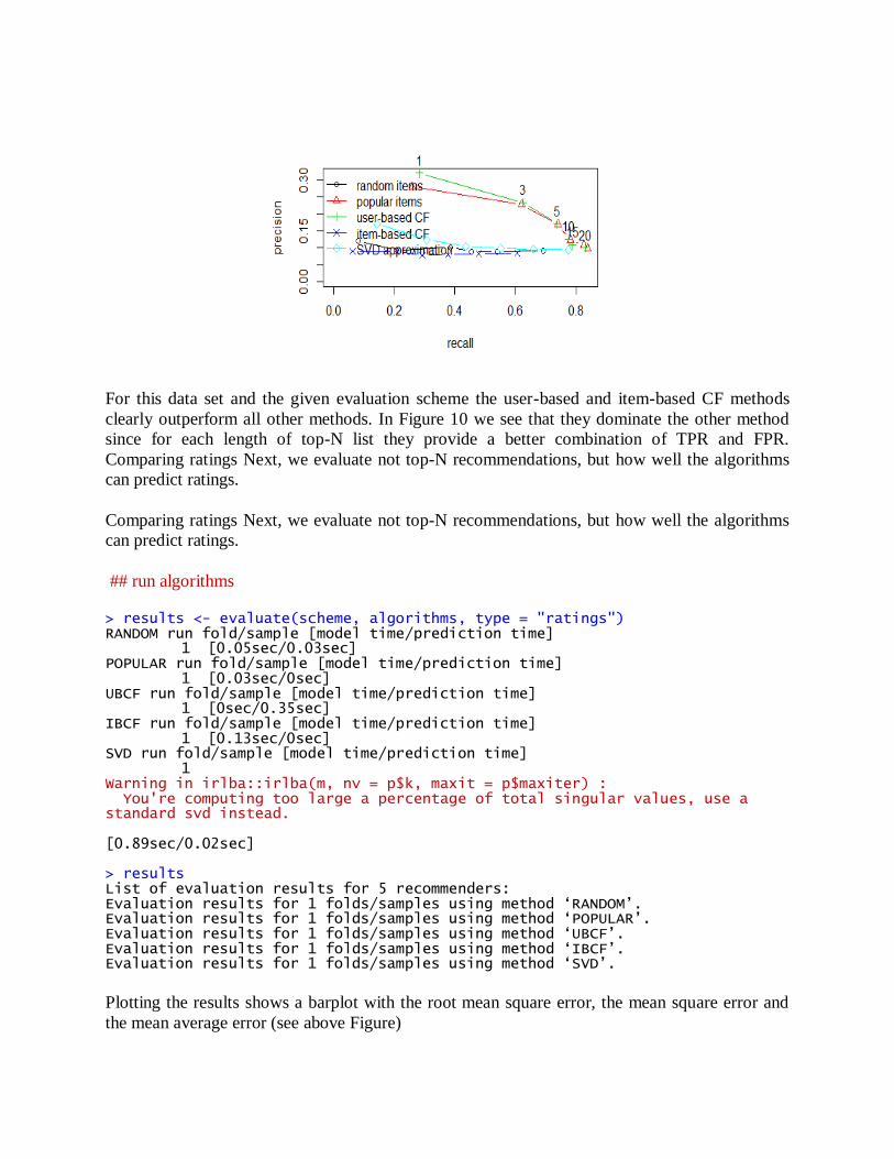
For this data set and the given evaluation scheme the user-based and item-based CF methods

clearly outperform all other methods. In Figure 10 we see that they dominate the other method

since for each length of top-N list they provide a better combination of TPR and FPR.

Comparing ratings Next, we evaluate not top-N recommendations, but how well the algorithms

can predict ratings.

Comparing ratings Next, we evaluate not top-N recommendations, but how well the algorithms

can predict ratings.

## run algorithms

> results <- evaluate(scheme, algorithms, type = "ratings") RANDOM run fold/sample [model time/prediction time] 1 [0.05sec/0.03sec] POPULAR run fold/sample [model time/prediction time] 1 [0.03sec/0sec] UBCF run fold/sample [model time/prediction time] 1 [0sec/0.35sec] IBCF run fold/sample [model time/prediction time] 1 [0.13sec/0sec] SVD run fold/sample [model time/prediction time] 1 Warning in irlba::irlba(m, nv = p$k, maxit = p$maxiter) : You're computing too large a percentage of total singular values, use a standard svd instead. [0.89sec/0.02sec] > results List of evaluation results for 5 recommenders: Evaluation results for 1 folds/samples using method ‘RANDOM’. Evaluation results for 1 folds/samples using method ‘POPULAR’. Evaluation results for 1 folds/samples using method ‘UBCF’. Evaluation results for 1 folds/samples using method ‘IBCF’. Evaluation results for 1 folds/samples using method ‘SVD’.

Plotting the results shows a barplot with the root mean square error, the mean square error and

the mean average error (see above Figure)

Using a 0-1 data set For comparison we will check how the algorithms compare given less

information. We convert the data set into 0-1 data and instead of a all-but-5 we use the given-3

scheme.

> Jester_binary <- binarize(Jester5k, minRating=5) > Jester_binary <- Jester_binary[rowCounts(Jester_binary)>20] > Jester_binary 1797 x 100 rating matrix of class ‘binaryRatingMatrix’ with 65642 ratings.

> scheme_binary <- evaluationScheme(Jester_binary[1:1000], + method="split", train=.9, k=1, given=3) > scheme_binary Evaluation scheme with 3 items given Method: ‘split’ with 1 run(s). Training set proportion: 0.900 Good ratings: NA Data set: 1000 x 100 rating matrix of class ‘binaryRatingMatrix’ with 36468 ratings. > results_binary <- evaluate(scheme_binary, algorithms, + + type = "topNList", n=c(1,3,5,10,15,20)) RANDOM run fold/sample [model time/prediction time] 1 [0.02sec/0.03sec] POPULAR run fold/sample [model time/prediction time] 1 [0sec/0.56sec] UBCF run fold/sample [model time/prediction time] 1 [0sec/0.79sec] IBCF run fold/sample [model time/prediction time] 1 [0.15sec/0.06sec] SVD run fold/sample [model time/prediction time] 1 Timing stopped at: 0 0 0 Error in .local(data, ...) : Recommender method SVD not implemented for data type binaryRatingMatrix . Warning message: In .local(x, method, ...) : Recommender 'SVD approximation' has failed and has been removed from the results!

Note that SVD does not implement a method for binary data and is thus skipped.

> plot(results_binary, annotate=c(1,3), legend="topright")

9. Implementing a new recommender algorithm

Adding a new recommender algorithm to recommenderlab is straight forward since it uses a

registry mechanism to manage the algorithms. To implement the actual recommender algorithm

we need to implement a creator function which takes a training data set, trains a model and

provides a predict function which uses the model to create recommendations for new data. The

model and the predict function are both encapsulated in an object of class Recommender. For

examples look at the files starting with RECOM in the packages R directory. A good examples is

in RECOM_POPULAR.R.

Conclusion:- recommenderlab currently includes several standard algorithms and adding new

recommender algorithms to the package is facilitated by the built in registry mechanism to

manage algorithms.

Reference:- recommenderlab: A Framework for Developing and Testing Recommendation

Algorithms by Michael Hahsler SMU.

**************************************THE END*****************************