title leader‒follower navigation in obstacle environments

Title Leader‒Follower Navigation in Obstacle Environments WhilePreserving Connectivity Without Data Transmission

Author(s) Sakai, Daito; Fukushima, Hiroaki; Matsuno, Fumitoshi

Citation IEEE Transactions on Control Systems Technology (2018),26(4): 1233-1248

Issue Date 2018-7

URL http://hdl.handle.net/2433/232584

Right

© 2017 IEEE. Personal use of this material is permitted.Permission from IEEE must be obtained for all other uses, inany current or future media, including reprinting/republishingthis material for advertising or promotional purposes, creatingnew collective works, for resale or redistribution to servers orlists, or reuse of any copyrighted component of this work inother works.; This is not the published version. Please cite onlythe published version. この論文は出版社版でありません。引用の際には出版社版をご確認ご利用ください。

Type Journal Article

Textversion author

Kyoto University

IEEE TRANSACTIONS ON CONTROL SYSTEMS TECHNOLOGY, VOL. XX, NO. XX, JANUARY 20XX 1

Leader-Follower Navigation in ObstacleEnvironments While Preserving Connectivity

Without Data TransmissionDaito Sakai, Hiroaki Fukushima, Member, IEEE, and Fumitoshi Matsuno, Member, IEEE

Abstract—In this paper, we propose a control method forleader-follower navigation in obstacle environments while pre-serving sensing network connectivity without data transmissionbetween robots. Unlike most connectivity-preserving algorithms,the control input is determined in such a way as to not onlyguarantee connectivity preservation and collision avoidance, butalso to ensure input constraints are not violated at each timestep. We also introduce a simple rule for changing networktopology depending on environments such that some sensing linksare deactivated in order to pass through narrow spaces, whileactive links are increased in free spaces to keep the group ascohesive as possible. The effectiveness of the proposed method isdemonstrated in simulations and experiments.

Index Terms—Leader-follower navigation, connectivity main-tenance, collision avoidance, obstacle environment, line of sight.

I. INTRODUCTION

The cooperative control of multiple mobile robots hasbeen intensively studied for potential applications such asexploration, surveillance, mapping of unknown environments,and the transport of large objects (see, e.g., [1], [2], and [3] foran overview). This paper focuses on the fundamental problemof how to move a group of robots as a whole to a target area.Specifically, we assume that only one of the robots, called theleader, knows the path to the target area. Thus, since each robotin the group has a limited sensing and communication range,the connectivity of the sensing/communication network mustbe preserved in order to avoid leaving some robots behind.Furthermore, we aim to derive an algorithm without relyingon data transmission between robots, in order to deal withenvironments where there is no wireless network available forsuch information exchange.

Various methods for controlling multi-agent systems whilepreserving network connectivity have been proposed [4]–[24],as detailed in Section II (see also [25] for an overview).However, most of the previous methods have had at least oneof the following limitations.

1) An obstacle-free environment is considered [4]-[20].

This paper was supported in part by JSPS KAKENHI Grant Number15K06137.

D. Sakai is with Hitachi Construction Machinery Co., Ltd., Tsuchiura,Ibaraki 300-0013, Japan (e-mail: [email protected])

H. Fukushima and F. Matsuno are with the Department of MechanicalEngineering and Science, Graduate School of Engineering, Kyoto Univer-sity, Kyoto daigaku-Katsura, Nishikyo-ku, Kyoto 615-8540, Japan (e-mail:[email protected]; [email protected])

2) Data transmission between robots through a wirelessnetwork is required to estimate network connectivity[4]–[12], [22].

3) It is difficult to explicitly consider input constraints [4]–[17], [22]–[24].

4) A fixed network topology must be preserved or onlylinks can be added [13]–[17], [23], [24].

5) Inter robot collision is not considered [18]–[21].In this paper, we propose a control method for leader-

follower navigation in obstacle environments while preservingsensing network connectivity without data transmission be-tween robots. Unlike most connectivity-preserving algorithms,the control input is determined so as not only to guaranteeconnectivity preservation and collision avoidance, but alsoto ensure that a given input constraint is not violated ateach time step. Although an input constraint is considered inthe connectivity-preservation algorithm for the leader-followernavigation proposed in [20], it has limitations in that anobstacle-free environment is assumed and that collision avoid-ance is not guaranteed. In obstacle environments, the proposedmethod manages control input so as to preserve line-of-sight(LOS) visibility between neighbors as well as a maximumdistance constraint. We also derive conditions for collisionavoidance not only with robots that are visible at the currentsampling step, but also with those that are not visible, e.g.,due to an obstacle. Another key issue for leader-followernavigation in obstacle environments is how to move throughnarrow spaces without getting stuck. We introduce a simplerule to change network topology depending on environmentsin such a way that some sensing links are deactivated in orderto pass through narrow spaces while active links are increasedin free spaces to keep the group as cohesive as possible.Furthermore, unlike many other studies including [20], theeffectiveness of the algorithm is demonstrated not only withsimulations, but also in real robot experiments.

II. RELATED WORKS

In this section, we review previous studies on networkconnectivity preservation in multi-agent systems. Althoughmany control methods have been developed by assumingnetwork connectivity (see e.g. [26]-[38]), we do not focus onthese in this paper.

Many studies use the Fiedler value [39], which is thesecond smallest eigenvalue of the Laplacian matrix of thegraph describing the network, as a metric for overall network


connectivity. If the Fiedler value of a graph is positive, theconnectivity of the graph is guaranteed. Some early studiespresented centralized algorithms to increase the Fiedler valueof graphs. Kim and Mesbahi [4] proposed an iterative semidef-inite programming-based approach to maximizing the Fiedlervalue of the graph, while Zavlanos and Papas [5] reportedan artificial potential function-based approach to keeping theFiedler value positive.

One way to decentralize such algorithms is to make use of adecentralized estimation method of the connectivity [6]–[8], inwhich each agent estimates the eigenvalues (or eigenvectors)of the Laplacian matrix using information received fromneighbors. Based on the connectivity estimation, a gradientcontroller to maximize the Fiedler value was designed in[6] and [7], while an artificial potential function to keep theFiedler value positive was used in [9], [10], [22].

Although these algorithms based on the Fiedler value aretheoretically sophisticated, it is difficult to apply them to thecontrol problem described in Section I, since they requiredata transmission between robots (or between a central com-puter and each robot in the centralized algorithms [4], [5]),through wireless communication to exchange information onthe Laplacian matrix. Another limitation is the difficulty inexplicitly considering an input constraint. Furthermore, poorestimation of connectivity could lead to violation of networkconnectivity. To address this issue, Sabattini et al. [9] provedthe boundedness of estimation errors of the Fiedler value, andsuggested taking an estimation error bound into account inthe design of the artificial potential function. However, it isnot clear how to obtain such an error bound that is not tooconservative to apply to the artificial potential design.

In [11], an auction algorithm was implemented to decide co-operatively whether or not a link could be deactivated withoutviolating network connectivity. Zavlanos et al. [12] proposeda flocking algorithm that achieved velocity synchronizationof agents in a network while preserving connectivity using amethod similar to that in [11]. However, the auction algorithmrequired data transmission between robots to share informationon bids from other robots.

On the other hand, network connectivity preservation al-gorithms without data transmission between robots have alsobeen studied. In [13]–[17], [23], artificial potential functionswere used to preserve the initial network topology, whichwas assumed to be connected. In particular, connectivitypreservation in obstacle environments was considered in [23].Since these methods do not allow for the deactivation of anysensing link, it is difficult for robots to pass through narrowspaces if their initial network topology has many redundantlinks to make the group cohesive. Another limitation of thesemethods is that it is difficult to explicitly consider an inputconstraint. On the other hand, in [18]–[21], a given inputconstraint can be explicitly considered in the control design.

In [18], [19], [21], multi-robot rendezvous algorithms whilepreserving connectivity are proposed. In particular, obstacleenvironments are considered in [21]. With these algorithms,each robot computes at each time a convex region, calleda constraint set, in which the robot is constrained to movewithin this region to preserve sensing links with neighbors.

The robots then move towards the circumcenter of theirconstraint set. The amount of movement is determined suchthat no given input constraint is violated. However, movingtowards the circumcenter of the constraint set in order togather at the same location is not necessarily appropriatein the leader-follower navigation problem considered here.Another difference between our proposed control method andthese rendezvous algorithms is that we consider inter-robotcollisions. Thus, we need to consider the problem of how todeactivate sensing links in order for robots to pass throughnarrow spaces without getting stuck; this does not arise if inter-robot collisions are ignored. Furthermore, our method does notneed to compute a constrained set to determine control inputs,which results in decreased computation time.

The leader-follower navigation algorithm in [20] decides thedirection of movement using an artificial potential function,then the amount of movement is determined taking intoaccount the input constraint and network connectivity. We alsouse this basic procedure in our proposed method. However,[20] did not consider obstacle environments and inter-robotcollisions. To overcome this limitation, we derive additionalconstraints on the amount of movement so as to achieveLOS visibility preservation, obstacle avoidance and inter robotcollision avoidance. Furthermore, as already mentioned, weintroduce a link deactivation rule in order for robots to passthrough narrow spaces without getting stuck.

Panagou and Kumar [24] proposed a leader-follower nav-igation method in obstacle environments where the networktopology was fixed to a chain formation. As the distancebetween robots was controlled to a given constant value, theirmulti-robot system can be regarded as a tractor-trailer system.A limitation of this method is that as the number of robotsgrows, the turning radius of the leader must be increased, anda wider path is required. Furthermore, tracking error from atarget relative position is not guaranteed to converge to zero,and estimation of the error bound is difficult especially inthe case of multiple followers. If the tracking error is large,connectivity maintenance and collision avoidance might notbe achieved.

III. PROBLEM SETTING

We consider N robots in a two-dimensional work space withobstacles. The movement of the ith robot (i = 1, 2, . . . , N ) isdescribed as the following discrete-time system

xi(k + 1) = xi(k) + ui(k), ‖ui(k)‖ ≤ umax (1)

where xi(k) and ui(k) are the position and control input ofrobot i, respectively, at time step k (= 0, 1, . . .). The inputlimit umax in (1) is given by taking into account the hardwarelimitations and length of the sampling interval. We assume thata sufficient condition for collision avoidance between robots iand j is given as follows.

‖xi − xj‖ ≥ dc, ∀j ∈ V \ {i} (2)

where V := {1, 2, . . . , N} is the set of indices of all robots.Although a robot is modeled as a point in (1), dc in (2) shouldbe determined by taking into account the size of the actual


robots. We also assume that a sufficient condition for obstacleavoidance is given as

‖xi − xo‖ ≥ do, ∀xo ∈ O (3)

where O is a set of all points on obstacles in the workspace.In order to describe the sensing model, we first define the

line segment joining p and q as

L(p, q) := {(1− λ)p+ λq, ∀λ ∈ [0, 1]}. (4)

Furthermore, we define

Lij(k) := L(xi(k), xj(k)). (5)

Then, we assume that robot i is able to sense the relativeposition of robot j ∈ V \ {i}

xji(k) := xj(k)− xi(k) (6)

if the following conditions are satisfied

‖xj − xi‖ ≤ ds (7)‖q − xo‖ ≥ dl, ∀q ∈ Lij , ∀xo ∈ O. (8)

The condition in (7) implies that the maximum sensing rangeis given by a positive number ds. The condition in (8) impliesthat the distance from Lij to each obstacle is not less than aminimum clearance dl, so that the LOS between robots i andj is not interrupted by obstacles.

It is also assumed that robot i is able to detect a point onan obstacle xo ∈ O, if

‖xo − xi‖ ≤ ds (9)‖xo − xi‖ ≤ ‖q − xi‖, ∀q ∈ L(xi, xo) ∩ O (10)

where L(xi, xo) := {(1 − λ)xi + λxo, ∀λ ≥ 0}. While theset L(xi, xo) only includes points between xi and xo, the setL(xi, xo) includes points behind xo along the line from xi toxo, in addition to the points in L(xi, xo). Thus, the conditionin (10) implies that there is no other obstacle point closer toxi than xo on L(xi, xo). We denote Oi(k) as the set of pointson obstacles detected by robot i at time k.

In terms of the sensing mentioned above, we represent thenetwork topology of the multi-robot system using a graphGs(x(k)) = (V, Es(x(k))) where x = [x1, x2, . . . , xN ]. Wedenote V and Es(x(k)) as the node set and edge set, respec-tively. The elements of Es(x(k)) are pairs of robot indices thatare able to sense each other’s position at time k. The graph Gs

is said to be connected, if for every pair of nodes there existsa path from one node to the other.

We assume that a target path is given to only one of the Nrobots, called the leader, whose index is set as N withoutloss of generality. Other robots i (= 1, 2, . . . , N − 1) arecalled followers. It is assumed that each follower is not ableto recognize whether or not another robot is the leader. IfGs is connected, there is a path between the leader and eachfollower. Thus, since the maximum length of each link of Gs

is kept to no more than a given finite value ds, each followeris forced to follow the leader at a certain distance (at most(N − 1)ds). Furthermore, if the length of the link is kept toless than ds, the distance between the leader and a follower

can be decreased. Thus in this paper, we aim to preserve theconnectivity of the following subgraph of Gs(x(k)).

Gn(x(k)) := (V, En(x(k))) (11)En(x(k)) := {(i, j) ∈ Es(x(k)) | ‖xi(k)− xj(k)‖ ≤ dn}

where dc < dn < ds. Then, the set of neighbors of robot i isdefined as

Ni(x(k)) := {j | (i, j) ∈ En(x(k))}. (12)

From the definition of Gn(x(k)), the connectivity of Gs ispreserved if that of Gn(x(k)) is preserved. As clarified inTheorem 2 in Section IV-C, it is required that

√d2o + d2n ≤ ds

holds to guarantee the preservation of Gn. In other words,if dn = ds, i.e., Gn = Gs, it is difficult to guarantee thepreservation of Gs, which is another reason why we introduceGn in addition to Gs.

We assume that Gn is connected at the initial time k = 0.Thus, the simplest way to preserve connectivity is to controlthe robots such that the edges of Gn at k = 0 are not lost.However, in obstacle environments, it is often necessary tochange the network topology appropriately to navigate througha narrow space. Thus, it is necessary to select edges to bemaintained at each time step, such that the connectivity ofGn is preserved at the next time step. To describe the edgesto be preserved, we define the symmetric indicator functionσij(k) = σji(k) ∈ {0, 1}. If σij = 1, there will be an effortto preserve the edge (i, j). In other words, robot i aims topreserve the link to robot j in the following set

N σi (x(k)) := {j ∈ Ni(k) | σij(k) = 1}. (13)

We also define the following subgraph of Gn(x(k))

Gσ(x(k)) := (V, Eσ(x(k))) (14)Eσ(x(k)) := {(i, j) ∈ En(x(k)) | σij(k) = 1}. (15)

If σij is determined such that Gσ is connected, the connectivityof Gn is preserved by moving the robots in such a way thatno edge of Gσ is lost.

In this paper, we propose an algorithm to determine ui soas to preserve the connectivity of Gn, while satisfying thecollision avoidance conditions in (2) and (3). The proposedmethod aims to preserve these properties not only at xi(k)(k = 0, 1, . . .) but also at each point on the line segmentsL(xi(k), xi(k + 1)). It is reasonable to consider a path com-posed of line segments in the sense that a robot described by acommonly used continuous time model xi(t) = ui(t) followssuch a path when the control input ui(t) is fixed betweendiscrete time steps. Furthermore, the proposed algorithm aimsto determine σij in order to avoid deadlock in narrow spaces,while increasing active links to keep the group as cohesive aspossible if there are no obstacles around the robots.

Remark 1: In order to keep the notation as simple as possi-ble, the problem setting in this section and control algorithmin the next section are described by the global coordinates.However, for implementation, each robot determines the con-trol input vector using local coordinates. Global coordinatessuch as xi, xj and xo are replaced by local coordinates ixi,ixj and ixo in the control algorithm, where ixi = 0 since the


Fig. 1. Conditions for (i, j,m) ∈ T (left) and (i, j,m) ∈ T (right).

origin of robot i’s local frame is located at xi. The controlinput iui with respect to the local frame is obtained by thecontrol algorithm using the local coordinates. By applying iui

to the robot, the global input vector ui =0Riiui is applied

in (1), where 0Ri ∈ SO(2) denotes the orientation of roboti’s local frame with respect to the global frame. Therefore,the proposed algorithm can be implemented using only localinformation.

IV. CONTROL ALGORITHM

The outline of the control algorithm for robot i at time k isdescribed as follows.

Step 1: According to the sensing information on the relativeposition of robot j ∈ Ni, the indicator function σij(k) isdetermined, such that Gσ(x(k)) is connected.

Step 2: The direction of the control input vector ui(k) isdetermined based on an artificial potential function.

Step 3: The magnitude of ui(k), which guarantees the edgepreservation of Gσ(x(k)) and collision avoidance at each pointon L(xi(k), xi(k + 1)), is determined by taking into accountthe given input constraint in (1).

In the following subsections, we describe the details of eachstep.

A. Link Deactivation for Navigation in Narrow Spaces

By link deactivation, we mean deciding the edges of Gn

that will not be preserved. More precisely, we obtain the setEσ of preserved edges by removing some edges from En. Thereare two cases where an edge in En is not included in Eσ . Todescribe the first case, the following region is defined for givenxi, xj and xji in (6).

Dij :={q | (q − xi)

Txji > 0, (q − xj)Txji < 0

}(16)

as illustrated in Fig. 1 (left). We also define

ϕ(p, q) :=pTHq

‖Hq‖2Hq, H :=

[0 −11 0

](17)

which is the projection of a vector p to the line orthogonal toq. Thus, as shown in Fig. 1 (left), ‖ϕ(xmi, xji)‖ is the distancefrom xm to the line including xi and xj . Then, we define Tas the set of triples of robots (i, j,m) that satisfies

‖ϕ(xmi, xji)‖ ≤ ddel, xm ∈ Dij , sinαm > 0 (18)(i, j) ∈ En, (j,m) ∈ En, (m, i) ∈ En (19)

where ddel is a positive constant satisfying

ddel < dc sinπ

3. (20)

In (18), αm ∈ (−π, π] denotes the angle from the vectorxim to xjm measured in the counter-clockwise direction. Thecondition sinαm > 0 implies that the triple vertices in T areordered in a counter-clockwise direction, as shown in Fig. 1(left). Then, robot i does not include the edge (i, j) ∈ En inEσ if

(i, j,m) ∈ T or (j, i,m) ∈ T , ∃m ∈ V \ {i, j}. (21)

If the condition in (20) and the collision avoidance condition in(2) are satisfied, it is guaranteed that the links (j,m) and (m, i)of the robots (i, j,m) satisfying (21) will not be deactivated,as shown in Lemma 3 in Appendix A. Therefore, the networkconnectivity is preserved at least if N = 3, i.e., if there are norobots other than (i, j,m). Furthermore, Theorem 1 discussesconnectivity in the case of N > 3. On the other hand, if (20)is violated, the preservation of connectivity is not guaranteedeven if N = 3. For example, if ddel = dc sin

π3 , all the links

among the robot triple (i, j,m) will be deactivated, when theirpositions constitute an equilateral triangle with edge length dc.

To describe the other case where an edge is removed fromEσ, we define T as the set of robot triples (i, j,m) that satisfy

‖xij‖ = ‖xjm‖ = dn, ‖xmi‖ = dc, sinαm > 0 (22)

and (19). As illustrated in Fig. 1 (right), a robot triple(i, j,m) ∈ T forms an isosceles triangle with two edges oflength dn and one edge of length dc. In the edge deletion rulein this paper, robot i does not include the edge (i, j) ∈ En inEσ if

(i, j,m) ∈ T or (j, i,m) ∈ T , ∃m ∈ V \ {i, j}. (23)

In summary, the rule to decide σij is described as follows.

σij(k) =

{0, if (21) or (23),1, otherwise.

(24)

This rule is decentralized and does not require data transmis-sion between robots. We obtain the following result on theconnectivity of Gσ when multiple links are deleted at the sametime by the rule in (24).

Theorem 1: Suppose A1) Gn(x(k)) is connected, A2) allrobots satisfy the collision avoidance conditions in (2)-(3) attime k, A3) the condition in (20) is satisfied, and A4) π isnot an integer multiple of sin−1(dc/2dn). Then, Gσ(x(k))obtained by the rule in (24) is connected.

Proof: See Appendix A.Remark 2: Since the equalities in (22) do not hold exactly

in practice, we instead check if the following inequalities

dn − εn ≤ ‖xij‖ ≤ dn, dn − εn ≤ ‖xjm‖ ≤ dn

dc ≤ ‖xmi‖ ≤ dc + εc

are satisfied for small positive constants εn and εc.


0.3 0.4 0.5 0.6 0.7 0.8 0.9 1 1.10

2

4

6

8

10

z

Φcol (z)

Fig. 2. Example of Φcol(z) (dc = 0.3, dr = 0.7, dn = 1.0).

B. Direction of Control Input Vector

For the leader (i = N ), the direction of ui(k), which isequivalent to the robot’s direction of movement, is given fromthe target path in the same way as described in [20]. For thefollowers, on the other hand, the direction of the movement isdecided by

vi = −∇xiΨi(x), i ∈ V \ {N} (25)

where Ψi(x) is the artificial potential function defined below.Note that vi in (25) can be computed using only local infor-mation, since Ψi(x) depends only on a part of the elementsof x, i.e., xi and xj (j ∈ N σ

i ).The artificial potential function Ψi(x) is a weighted sum of

Ψcoli , Ψobs

i , Ψlosi and Ψcoh

i as follows

Ψi := c1Ψcoli + c2Ψ

obsi + c3Ψ

losi + c4Ψ

cohi . (26)

The first component Ψcoli takes into account the desired value

and constraints on the relative distance to neighbors j ∈ N σi .

Artificial potential functions for this purpose are available inthe literature. In this paper, we adopt a similar function to thatin [17], as follows:

Ψcoli (x) =

∑j∈Nσ

i

Φcol(‖xi − xj‖) (27)

Φcol(z) :=(z − dr)

2(dn − z)

(dn − dc)2(z − dc) + (dr − dc)2(dn − z)/κ1

+(z − dc)(z − dr)

2

(dn − dc)2(dn − z) + (z − dc)(dn − dr)2/κ2

where κ1 and κ2 are design parameters whose values areequivalent to Φcol(z) at z = dc and z = dn, respectively. Fig. 2illustrates an example of Φcol(z) for dc = 0.3, dr = 0.7, dn =1.0, κ1 = κ2 = 10. As shown in this example, Φcol(z) hasthe minimum value at the desired relative distance dr, andmonotonically increases as z goes to the maximum allowabledistance dn, or to the minimum allowable distance dc.

The second component Ψobsi (x) is introduced for obstacle

avoidance. More precisely, Ψobsi (x) is decided in such a way

that −∇xiΨobsi (x) is in the direction away from the closest

obstacle point detected at time k. Such an obstacle point isdefined as

oobsi = arg minxo∈Oi(k)

‖xo − xi(k)‖. (28)

0 0.1 0.2 0.3 0.4 0.50

2

4

6

8

10

z

Φobs (z)

Fig. 3. Example of Φobs(z) (do = 0.1, dor = 0.2).

By using oobsi above, Ψobsi (x) is described as

Ψobsi (x) = Φobs(‖xi − oobsi ‖)

Φobs(z) =

12

((z−do

dor−do+ δ

)−1

− 11+δ

)2

, if z < dor

0, otherwise

where dor > do is a design parameter, and δ is a small numberto keep Φobs(z) finite. Fig. 3 presents an example of Φobs(z)for do = 0.1, dor = 0.2. As shown in this example, Φobs(z)monotonically increases as z goes from dor to the minimumallowable distance do to obstacles.

The third component Ψlosi (x) is decided in such a way that

−∇xiΨlosi (x) is in the direction moving away from the closest

point to Lij(k) among the obstacle points in Dij detected attime k. Such an obstacle point is defined as

olosij = arg minxo∈Oi∩Dij

‖ϕ(xoi, xji)‖. (29)

We also define

j∗ = arg minj∈Nσ

i

‖olosij ‖. (30)

By using olosij and j∗ above, Ψlosi (x) can be described as

Ψlosi (x) = Φlos(‖ϕ(xi − olosij∗ , xi − xj∗)‖)

Φlos(z) =

12

((z−dl

dlr−dl+ δ

)−1

− 11+δ

)2

, if z < dlr

0 , otherwise.

In the same way as Φobs(z), the value of Φlos(z) monoton-ically increases as z goes from dlr to the minimum allow-able distance dl from Lij to obstacles. Thus, the component−∇Ψlos

i (x) of vi in (25) has the effect of moving Lij awayfrom its closest obstacle point.

The fourth component Ψcohi (x) is introduced to make the

group more cohesive. More precisely, Ψcohi (x) is decided such

that −∇xiΨcohi (x) is in the direction of moving closer to


neighbors whose distance from robot i is more than dn whenthere is no obstacle around, i.e.,

Ψcohi (x) =

∑j∈Si

Φcoh(‖xi − xj‖)

Φcoh(z) =

{12 (z − dn)

2 , if ‖z‖ > dn,Oi = ∅0 , otherwise.

(31)

C. Magnitude of Control Input Vector

In this section, we determine ‖ui(k)‖ (i = 1, . . . , N )so as to achieve the preservation of Eσ(x(k)) and collisionavoidance. It should be noted that the leader and followers usethe same algorithm to determine ‖ui(k)‖, unlike the directionof ui(k) in Section IV-B.

As mentioned in Section III, the proposed method aims toachieve connectivity preservation and collision avoidance notonly at xi(k) for each discrete time k (k = 0, 1, . . .) but also ateach point on the line segment connecting xi(k) and xi(k+1),i.e., pi ∈ Pi(k) := L(xi(k), xi(k + 1)). To this end, we firstpresent an upper bound for ‖ui(k)‖ to satisfy the followingconditions.

i) The maximum distance condition for each j ∈ N σi (k)

‖pi − pj‖ ≤ dn, ∀pi ∈ Pi(k), ∀pj ∈ Pj(k). (32)

ii) The inter-robot collision avoidance condition for eachj ∈ Si(k)

‖pi − pj‖ ≥ dc, ∀pi ∈ Pi(k), ∀pj ∈ Pj(k). (33)

iii) The obstacle avoidance condition for each xo ∈ Oi(k)

‖pi − xo‖ ≥ do, ∀pi ∈ Pi(k). (34)

iv) The LOS preservation condition for each j ∈ N σi (k)

‖q − xo‖ ≥ dl, ∀xo ∈ O, ∀q ∈ L(pi, pj)∀pi ∈ Pi(k), ∀pj ∈ Pj(k). (35)

Note that the upper bound of ‖ui(k)‖ to satisfy i) is derivedin [20] without taking into account obstacles and collisions,while our goal here is to guarantee i)-iv) at the same time inobstacle environments. It also should be noted that conditions(33)-(34) must be satisfied for any j ∈ V \ {i} and xo ∈ O inorder to avoid collision with any robot or obstacle point. Thus,we further derive conditions where (33)-(34) are satisfied forj 6∈ Si and xo 6∈ Oi.

The condition in [20] for ui(k) to satisfy i) is described asfollows.

‖ui(k)‖ ≤ 1

2

(dn − max

j∈Nib(k)‖xji(k)‖

)=: ucon1

i (k) (36)

‖ui(k)‖2 ≤ minj∈Nif (k)

{uTi (k)xji(k)

}. (37)

In these conditions, Nib(k) denotes the set of robots j ∈ N σi

from which robot i will move away at time k + 1, i.e.,

Nib(k) ={j ∈ N σ

i (k)|vTi (k)xji(k) ≤ 0}

(38)

and Nif (k) denotes the rest of the robots j ∈ N σi (k), i.e.,

Nif (k) ={j ∈ N σ

i |vTi (k)xji(k) > 0}. (39)

Fig. 4. Input bound uobsi .

In other words, Nib is the set of robots behind robot i withrespect to the direction of the movement of robot i, while Nif

is the set of robots in front of robot i. Since ui is describedas

ui(k) = ‖ui(k)‖vi(k)

‖vi(k)‖(40)

using the vector vi(k) given in Section IV-B, the condition in(37) can be rewritten as

‖ui(k)‖ ≤ 1

‖vi(k)‖min

j∈Nif (k)

{vTi (k)xji(k)

}=: ucon2

i (k).

In order to describe a condition for ii), we first decomposethe set of robots Si(k) detected by robot i into the followingtwo sets

Sib(k) ={j ∈ Si(k)| vTi (k)xji(k) ≤ 0

}(41)

Sif (k) ={j ∈ Si(k)| vTi (k)xji(k) > 0

}. (42)

Using Sif (k), an upper bound for ‖ui(k)‖ is given as

ucoli (k) =

1

2

(min

j∈Sif (k)‖xji(k)‖ − dc

). (43)

An upper bound of ‖ui(k)‖ to satisfy iii) is given as

uobsi = max

s≥0{‖svi‖ | ‖xoi − svi‖ ≥ do, ∀xo ∈ Oi} (44)

where xoi := xo − xi. This upper bound allows robot i toproceed in the direction of vi, unless the distance to the closestobstacle point is less than do, as indicated in Fig. 4. It shouldbe noted that exact maximization on the right-hand side of (44)is difficult for general obstacle environments. An approximatevalue of uobs

i can be obtained by discretizing s and xo in(44). Another way is to approximate obstacles by a simpleshape such as circles, for which the maximum in (44) can beanalytically obtained (see Appendix D).

In order to describe the input bound ulosi for iv), we define

the set of detected obstacle points in Dij , toward which roboti will move closer at k + 1, as follows.

Olosijf (k) :=

{xo ∈ Oi ∩Dij | vTi ϕ(xoi, xji) > 0

}. (45)

If Olosijf (k) = ∅, no upper bound for ‖ui(k)‖ is given, i.e.,

ulosi = ∞. If Olos

ijf (k) 6= ∅, we define the closest obstaclepoint in Dij to Lij(k) as

olosij = arg minxo∈Olos

ijf

‖ϕ(xoi, xji)‖ (46)


Fig. 5. Input bound ulosij .

as illustrated in Fig. 5. Then, an upper bound for ‖ui(k)‖ isgiven as

ulosi = min

j∈Nσi

ulosij (47)

ulosij = max

s≥0

{‖svi‖ | ‖ϕ(olosij − xi − svi, xji)‖ ≥ dl

}.

As illustrated in Fig. 5, ulosij is the maximum allowable distance

of movement, such that the distance from robot i to theobstacles in the direction orthogonal to Lij(k) is not less thandl at time k + 1. Thus, ulos

ij is obtained as

ulosij =

‖ϕ(olosij − xi, xji)‖ − dl

sin θij(48)

where θij ∈ [0, π] is the angle between Lij and vi. An upperbound for ‖ui(k)‖ to satisfy i)-iv) is now given as

ui = min{ucon1i , ucon2

i , ucoli , uobs

i , ulosi , umax

}. (49)

Therefore, we determine ui(k) as follows

ui(k) =

{ui(k)

vi(k)‖vi(k)‖ , if ‖vi(k)‖ > ui(k)

vi(k), otherwise.(50)

Note that since ui is computed using positions of detectedrobots and obstacles and since the sensing range of each robotis limited, the computation time for each robot does not growas the total number of robots and obstacles increases.

Theorem 2: Suppose that collision avoidance constraints in(2)-(3) are satisfied for all robots at time k. Then, ui(k) in(50) satisfies i)-iv) for each robot i ∈ V , if

umax ≤ do − dl,√d2o + d2n ≤ ds (51)

in addition to (20).Proof: See Appendix B.

It should be noted that the control algorithm satisfying i)-iv) does not necessarily guarantee that (33)-(34) are satisfiedfor j 6∈ Si and xo 6∈ Oi. Thus, a collision with a robot hidingbehind an obstacle at time k could possibly arise at time k+1.To guarantee collision avoidance with robots j 6∈ Si(k) andobstacle points xo 6∈ Oi, additional conditions are required asshown in the following theorem.

Fig. 6. Obstacle environment in simulations for M = 2.

0

20

40

60

80

100

Rat

e of

case

s w

ith

out

dea

dlo

ck [

%]

0.2 0.3 0.4 0.5 0.6Width of path 2η [m]

Without link

deactivation

With link deactivation

Fig. 7. Rate of cases without deadlock for M = 0.

Theorem 3: In addition to the assumptions in Theorem 2,we assume

umax ≤ min

{ds2,√d2o − d2l

}− dc

2. (52)

Then, the inter-robot collision avoidance condition in (33) isguaranteed for each j ∈ V \ Si(k). Furthermore, if

umax ≤ ds − do (53)

the obstacle avoidance condition in (34) is guaranteed for eachxo ∈ O \ Oi(k).

Proof: See Appendix C.Remark 3: For the leader, umax in (49) might be replaced

by a smaller value ulmax, since it improves the cohesion of the

group, i.e., more edges are generated in En. In other words, ifthe leader moves at the maximum speed, i.e., ‖ui‖ = umax,it is difficult for pairs of robots (i, j) 6∈ En to decrease theinter-robot distance and to generate an edge in En.

While conditions for connectivity preservation and collisionavoidance are derived in Theorems 1–3, it is difficult toclarify conditions to ensure that no robots get stuck in narrowspaces. In the next section, we demonstrate the effectivenessand limitations of the proposed method by simulations undervarious conditions.


V. SIMULATION

In this section, we run various simulations to demonstratethe effectiveness of the proposed method. The values of theparameters defined in Section III are N = 10, ds = 2 m, dn =1 m, dc = 0.3 m, do = 0.1 m, dl = 0.05 m, and umax = 0.01m. The coefficients in (26) are set as c1 = 0.5, c2 = c3 = 0.01,and c4 = 5. The parameters in the artificial potential functionsin Section IV-B are set as κ1 = κ2 = 10, dr = 0.7, dor = 0.2,dlr = 0.1, and δ = 0.02. We set ddel = 0.25, εn = 0.1dn, andεc = 0.1dc for link deletion, and ul

max = 23umax to improve

the cohesion of the group, as mentioned in Remark 3.In order to measure the connectivity of the graph Gσ , we

compute the Fiedler value [39], which is the second smallesteigenvalue of the Laplacian matrix L. The Laplacian matrixL is defined as

L = ∆−A (54)

by using the adjacency matrix A, whose elements Aij are 1 if(i, j) ∈ Eσ and 0 otherwise, and a diagonal matrix ∆, whosediagonal elements are ∆i =

∑Nj=1 Aij (i = 1, . . . , N ).

Obstacle environments for simulations are illustrated in Fig.6. The target path of the leader is a series of connected linesegments starting at the origin, as shown in the thick solidlines. Obstacles are placed on both sides of the path. Therelative angle of the ith line segment from i−1th line segmentis defined as φi 6= 0 for i = 1, . . . ,M , if M ≥ 1. Thus,M represents the number of corners of the target path. Thefirst and last line segments can be divided into parts insideand outside the obstacle area. We define `s and `f as thelengths of the parts outside the obstacle area on the first andlast line segments, respectively. Furthermore, the length of theith line segment inside the obstacle area is defined as `i fori = 0, 1, . . . ,M .

The minimum distance between an obstacle and the leader’starget path is defined as η, which implies that obstacles shouldnot be in the area between two dashed lines. Subject to thisminimum distance constraint, we place circular obstacles sothat obstacles are as dense as possible to make the problemchallenging. To this end, each obstacle is placed so that thedistance from an obstacle to the leader’s target path is equal tothe allowable value η. In other words, the centers of circularobstacles with radius ro are placed on a dash-dotted line inFig. 6, which is at a distance of η+ro from the target path. Wealso set distance between the centers of neighboring obstacles,ρ, as a small value so that the density of obstacles is high.Furthermore, we located additional obstacles with a radiussmaller than ro at the inside corners, making the problem evenmore difficult. Specifically, we set ro = 0.5 m and ρ = 0.2 m,while the radii of small obstacles at the inside corners were0.1 m and 0.01 m.

We first tested the proposed method in the case where thetarget path of the leader was a straight line, i.e., M = 0. Thiswas to examine the effectiveness of the link deactivation rulein Section IV-A. If the target path has corners, it is possible forrobots to get stuck for a reason not necessarily related to theproposed link deactivation rule, as will be shown later. Thus,simulations with a straight path are suitable for investigating

Without link deactivation

(φ1=π/2, l0 =1)

φ1=π/2, l0 =1

φ1=π/2, l0 =10

φ1=π/6, l0 =1

φ1=π/6, l0 =10

0

20

40

60

80

100

Rat

e o

f ca

ses

wit

hou

t d

ead

lock

[%

]

0.3 0.4 0.5 0.6 0.7

Width of path 2η [m]

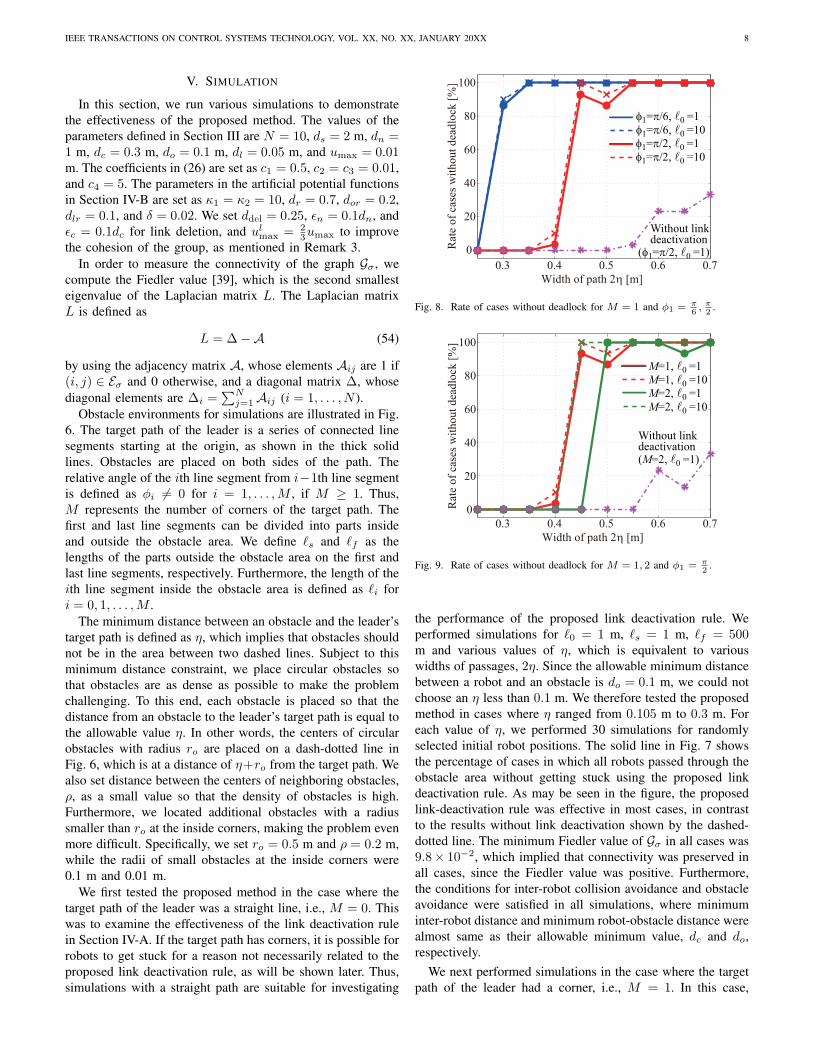
Fig. 8. Rate of cases without deadlock for M = 1 and φ1 = π6, π2

.

0

20

40

60

80

100

Rat

e o

f ca

ses

wit

ho

ut

dea

dlo

ck [

%]

0.3 0.4 0.5 0.6 0.7

Width of path 2η [m]

Without link deactivation(M=2, l0 =1)

M=1, l0 =1

M=1, l0 =10

M=2, l0 =1

M=2, l0 =10

Fig. 9. Rate of cases without deadlock for M = 1, 2 and φ1 = π2

.

the performance of the proposed link deactivation rule. Weperformed simulations for `0 = 1 m, `s = 1 m, `f = 500m and various values of η, which is equivalent to variouswidths of passages, 2η. Since the allowable minimum distancebetween a robot and an obstacle is do = 0.1 m, we could notchoose an η less than 0.1 m. We therefore tested the proposedmethod in cases where η ranged from 0.105 m to 0.3 m. Foreach value of η, we performed 30 simulations for randomlyselected initial robot positions. The solid line in Fig. 7 showsthe percentage of cases in which all robots passed through theobstacle area without getting stuck using the proposed linkdeactivation rule. As may be seen in the figure, the proposedlink-deactivation rule was effective in most cases, in contrastto the results without link deactivation shown by the dashed-dotted line. The minimum Fiedler value of Gσ in all cases was9.8× 10−2, which implied that connectivity was preserved inall cases, since the Fiedler value was positive. Furthermore,the conditions for inter-robot collision avoidance and obstacleavoidance were satisfied in all simulations, where minimuminter-robot distance and minimum robot-obstacle distance werealmost same as their allowable minimum value, dc and do,respectively.

We next performed simulations in the case where the targetpath of the leader had a corner, i.e., M = 1. In this case,


−2 0 2

−1

0

1

2

X

Y

−1 0 1 2 3

−1

0

1

2

X

Y

0 2 4−2

0

2

X

Y

0 2 4

−2

0

2

X

Y

2 4 6

−2

0

2

4

X

Y

4 6 8 10

−2

0

2

4

X

Y

12 14 16

0

2

4

X

Y

20 22 24

0

2

4

X

Y

k=200 k=700 k=1500 k=2000

k=2500 k=3000 k=4000 k=5000

Fig. 10. Snapshots of a simulation.

even if sensing links were properly deactivated to go througha path, robots could get stuck at the corner. To illustrate thisproblem, we show simulation results in the case of `0 = 10m, where the first straight path in the obstacle area is long.The dashed lines in Fig. 8 show that the percentage of caseswhere all robots passed through the obstacle area for `1 = 1.5,`s = 1 m, and `f = 500 m. It can be seen from this result thatrobots got stuck in many cases of 2η = 0.25 and 2η ≤ 0.4for φ1 = π/6 rad and φ1 = π/2 rad, respectively. This isin contrast that all robots passed through the obstacle areain most cases of 2.1 ≤ 2η ≤ 0.4 for a straight path, asshown in Fig. 7. Note that since we set N = 10 and dn = 1m, the distance between the first and last robots is no morethan 9 m. Thus, when the first robot reaches the corner inthe case of `0 = 10, all the robots are in the narrow pathafter the link deactivation has been successfully completed atthe entrance of the narrow space. Therefore, this difference ofresults for 2η ≤ 0.4 in Fig. 7 compared with Fig. 8 illustratesthat robots got stuck at a corner although the link deactivationwas successfully completed. A reason why this problem arisesis that the distance between two neighboring robots is too longto make a turn while preserving the LOS. Furthermore, thesolid lines in Fig. 8 show that the possibility of getting stuckis increased for `0 = 1 m, where the link deactivation hasnot been completed when some robots reach the corner. Onereason for this is that the velocity of robots around an entranceof the narrow space is decreased during link deactivation. Thismakes it difficult for the robots in front to move forward. Asa result, the distance between robots at the corner becomeslonger than that in the case of `0 = 10. Similarly, the rate ofgetting stuck is increased as the number of corners increases.Fig. 9 compares the cases of M = 1 and M = 2 wherewe set φ1 = π/2, φ2 = −π/2, `1 = `2 = 1.5 m. Asshown in this figure, the rate of getting stuck is higher for

M = 2. The limitation in making turns at narrow cornersmight be improved by modifying the direction of movement inSection IV-B so that the distance between robots is decreasedat corners, although that is beyond the focus of this paper.Despite this limitation, the simulation results show that therobots can successfully go through paths in most cases of2η ≥ 0.5 where it is still difficult to navigate without linkdeactivation. It should be also noted that the conditions forconnectivity preservation, inter-robot collision avoidance, andobstacle avoidance were satisfied in all examples shown in thissection, regardless of whether the paths have corners or not.Fig. 10 shows snap shots of the case where M = 2, whichillustrate that the robots are able to pass through narrow spacesby decreasing the number of active links, and then can increasethe active links in free space. However, there is a limitationthat regrouping into a cohesive formation takes quite a longtime since it is difficult to start regrouping before the lastrobot clears the obstacle area. One reason for this is that theleader (the first robot) does not consider group cohesion inthe control law. Thus, in order to improve the cohesion of thegroup, followers need to catch up with the leader. However, thefollowers other than the last robot cannot easily get closer tothe leader, since they need to keep the maximum allowabledistance dn with the neighbor behind as well as in front.Therefore, regrouping is not triggered until the last robot getscloser to the neighbor in front, after it clears the obstacle area.

VI. EXPERIMENT

The proposed method was applied to a group of 7 robots.For each robot, we used a mobile robot platform (Kobuki,Yujin Robot). Since the robots were not omni-directional, theirorientation was controlled in the direction of the control inputui before moving forward. The position and orientation of eachrobot were measured by a motion capture system (OptiTrack


−3 −2 −1 0 1 2

−2

−1.5

−1

−0.5

0

0.5

1

1.5

x

y

Fig. 11. Initial positions of robots (experiment).

0 200 400 600 8000

0.5

1

1.5

2

k

Fie

lder

Valu

e

Fig. 12. Fiedler value of the graph (experiment).

s250e) in a centralized way. Obstacle avoidance was simulatedusing virtual obstacles whose positions were known to therobots. However, only local information that could be obtainedin the sensing model in Section III was used to compute thecontrol input in order to simulate the decentralized algorithm.Experimental validation using on-board sensors is planned forfuture research.

The control algorithm was implemented every 0.5 sec. Thevalues of the parameters in Section III were ds = 1.6 m, dn =0.8 m, dc = 0.4 m, do = 0.3 m, dl = 0.2 m, and umax = 0.04m. The coefficients in (26) were set to c1 = 0.6, c2 = 0.1, andc3 = c4 = 1. Parameters in the artificial potential functionswere set to κ1 = κ2 = 100, dr = 0.7, dor = dlr = 0.4, andδ = 0.02. We set ddel = 0.3 for link deletion in (21) andulmax = 2

3umax to improve the cohesion of the group.As shown in Fig. 11, the virtual obstacles formed an L-

shaped path. The initial positions of the leader and followersare indicated by blue and red circles, respectively. As shownin Fig. 12, the Fiedler value of Gσ was always positive, whichimplies that connectivity was preserved. Fig. 13 shows thatinter-robot distances (solid line) did not violate the minimumallowable value dc (dashed line). Furthermore, as shown inFig. 14, the distances to obstacles did not violate the minimumallowable value do. Snap shots of the experiment are shownin Fig. 15, where the red lines in each photo represent the L-shaped path formed by the virtual obstacles. This figure shows

0 200 400 600 8000

0.2

0.4

0.6

k

Min

imu

m i

nte

r−ro

bot

dis

tan

ce

Fig. 13. Minimum inter-robot distance (experiment).

0 200 400 600 8000

0.1

0.2

0.3

0.4

0.5

k

Min

imum

dis

tance t

o o

bsta

cle

Fig. 14. Minimum distance to obstacles (experiment).

that the robots traversed the L-shaped path by deactivatinglinks to be preserved.

VII. CONCLUSIONS

This paper has presented a network connectivity preserva-tion method for leader-follower navigation in obstacle envi-ronments that explicitly takes an input constraint into account.We derived conditions for the proposed method to guaranteeconnectivity preservation and collision avoidance in the pres-ence of obstacles. A deactivation rule of sensing links, whichuses only local sensing information to preserve global networkconnectivity, was introduced to allow the robots to navigatenarrow spaces without getting stuck. The effectiveness of theproposed method was demonstrated by simulations and inexperiments. Future research will address the problem thatrobots may get stuck in a corner even if sensing links areproperly deactivated depending on the width of the path. Thealgorithm should also be improved so as to regroup robots intoa cohesive formation more rapidly in free spaces.

APPENDIX APROOF OF THEOREM 1

To prove Theorem 1 by contradiction, suppose that Gσ isnot connected, under Assumptions A1)-A4) in Theorem 1.

From Assumption A1), Gn is connected. Thus, there existsat least one pair of robots, i and j of Gσ , such that all thepaths connecting them are lost by applying the rule in (24),


Fig. 15. Snapshots of an experiment.

Fig. 16. Example of the case where all paths between two robots AI(1) andBI(1) are lost by deactivation rule in (24).

while i and j have an edge in Gn, i.e., (i, j) ∈ En. Thisimplies that robots i, j and another one m satisfy (21) or(23), so that (i, j) is deactivated by the rule in (24). Wedenote this robot triple by (Ah1 , Bh1 , Ch1), where h1 = 1in the case of (Ah1 , Bh1 , Ch1) ∈ T as in (23) while h1 = 2in the case of (Ah1 , Bh1 , Ch1) ∈ T as in (21). Then, theedge (Ah1 , Bh1) is deactivated by the rule in (24), regardlessof h1 = 1 or h1 = 2. Therefore, if neither the edge(Ah1 , Ch1) nor (Bh1 , Ch1) is deactivated, there still exists apath Ah1Ch1Bh1 between Ah1 and Bh1 , i.e., between robots iand j. From Lemma 1, there are three cases where (Ah1 , Ch1)or (Bh1 , Ch1) is deactivated, under Assumptions A2)–A3).We define (A(h1,h2), B(h1,h2), C(h1,h2)) as the robot triple thatcauses such a deactivation, where h2 = 1, 2, or 3 correspond-ing to 1)–3) in Lemma 1 for (A,B,C) = (Ah1 , Bh1 , Ch1) and(A′, B′, C ′) = (A(h1,h2), B(h1,h2), C(h1,h2)). We also defineI(k) := (h1, h2, . . . , hk) in order to make the notation simple,which implies that

(A(h1,h2), B(h1,h2), C(h1,h2)) = (AI(2), BI(2), CI(2)). (55)

Although the edge (AI(2), BI(2)), which is equivalent to(Ah1 , Ch1) or (Bh1 , Ch1), is deactivated in each case of h2 =1, 2, 3, there still exists a path AI(2)CI(2)BI(2) between AI(2)and BI(2), if the edges (AI(2), CI(2)) and (BI(2), CI(2)) re-main. However, these edges can be deactivated, if there exists arobot triple (AI(3), BI(3), CI(3)) that satisfies 1)–3) in Lemma1 for (A,B,C) = (AI(2), BI(2), CI(2)) and (A′, B′, C ′) =

Fig. 17. Example of 1)–3) in Lemma 1. (A,B,C) ∈ T in 1) and 2a), while(A,B,C) ∈ T in 2b) and 3).

(AI(3), BI(3), CI(3)), where h3 = 1, 2, 3 corresponding to 1)–3) in Lemma 1. Similarly, (AI(µ), BI(µ), CI(µ)) (hµ = 1, 2, 3)is defined for µ ≥ 4 as the robot triple that deactivates theedge (AI(µ−1), BI(µ−1)) or (BI(µ−1), CI(µ−1)). Since thenumber of robots is finite, the length of such a sequence ofdeactivations is finite. Thus, the path between Ah1 and Ch1

is not lost, unless a sequence of robot triples for deactivationform a loop; i.e., unless there exist two positive integers µ1 andµ2 (µ1 < µ2) such that (AI(µ2), CI(µ2)) or (BI(µ2), CI(µ2)) isequivalent to (AI(µ1), BI(µ1)). As shown in Lemma 2, sucha loop is formed only if (AI(µ), BI(µ)) (µ = 1, 2, . . . , µ2)are each deactivated due to (AI(µ), BI(µ), CI(µ)) ∈ T , i.e.,hµ = 1 (µ = 1, 2, . . . , µ2), until a loop is formed, as illustratedin Fig. 16. To form such a loop without collision, it is thereforenecessary for 2π to be an integer multiple of 2 sin−1(dc/2dn),which contradicts Assumption A4).

A. Lemmas to Prove Theorem 1

In this section, we denote the distance between robots Aand B by AB, in order to simplify the notation.

Lemma 1: In addition to A2)–A3) in Theorem 1, we assumethat three out of N robots satisfy (A,B,C) ∈ T or T so thatthe edge (A,B) is deactivated by the rule in (24). Then, theedge (B,C) or (A,C) is also deactivated, if and only if at leastone of the following three conditions is satisfied, as illustratedin Fig. 17.

1) There exists a robot triple (A′, B′, C ′) ∈ T that deacti-vates the edge (B,C), which is equivalent to (A′, B′).

2) There exists a robot triple (A′, B′, C ′) ∈ T that deacti-vates the edge (B,C), which is equivalent to (A′, B′).


3) There exists a robot triple (A′, B′, C ′) ∈ T that deacti-vates the edge (A,C), which is equivalent to (A′, B′).

Proof: We only prove the necessity, since the sufficiencyis obvious from the deactivation rule in (24).

From Lemma 3, we have (C,A,B) /∈ T and (B,C,A) /∈T , if (A,B,C) ∈ T . Also, it is obvious from the definition ofT that (C,A,B) /∈ T and (B,C,A) /∈ T if (A,B,C) ∈ T .Thus, the three robots (A,B,C) do not deactivate the edge(A,C) or (B,C) by themselves. In other words, (A,C) or(B,C) is deactivated, only if a robot other than (A,B,C)constitutes a triple (A′, B′, C ′) ∈ T or T , such that (A′, B′)is equivalent to (A,C) or (B,C).

We first consider the case of (A,B,C) ∈ T . Then, fromLemma 4, there is no robot triple (A′, B′, C ′) ∈ T thatdeactivates the edge (B,C) or (A,C), which is equivalentto (A′, B′). In other words, (B,C) or (A,C) is deactivatedonly if (A′, B′, C ′) ∈ T , as illustrated in 2b) and 3) of Fig.17.

In the case of (A,B,C) ∈ T , the edge (A,C) cannotbe deactivated as shown in Lemma 5. In other words, only(B,C) can be deactivated due to (A′, B′, C ′) ∈ T as in 1) or(A′, B′, C ′) ∈ T as in 2a) in Fig. 17.

Lemma 2: Under Assumptions A2–A3) in Theorem 1,there exist two positive integers µ1 and µ2 (µ1 < µ2)such that (AI(µ2), CI(µ2)) or (BI(µ2), CI(µ2)) is equivalentto (AI(µ1), BI(µ1)), only if hµ = 1 (µ = 1, 2, . . . , µ2).

Proof: To prove the contrapositive of the lemma, supposethat hµ 6= 1 for an integer µ (1 ≤ µ ≤ µ2). We defineµ (µ ≤ µ2) as the smallest positive integer µ satisfyinghµ 6= 1. Then, it follows from Lemma 4 that hµ 6= 1, i.e.,(AI(µ), BI(µ), CI(µ)) ∈ T , for µ < µ ≤ µ2. Thus, fromLemma 6, we have

AI(µ2)CI(µ2) < AI(µ2)BI(µ2)

BI(µ2)CI(µ2) < AI(µ2)BI(µ2). (56)

Since the edge (AI(µ2−1), CI(µ2−1)) or (BI(µ2−1), CI(µ2−1))is equivalent to (AI(µ2), BI(µ2)), it follows from (56) andLemma 6 that

AI(µ2)CI(µ2) < AI(µ2−1)BI(µ2−1)

BI(µ2)CI(µ2) < AI(µ2−1)BI(µ2−1). (57)

By repeating the same process, we have

AI(µ2)CI(µ2) < AI(µ)BI(µ)

BI(µ2)CI(µ2) < AI(µ)BI(µ) (58)

for µ ≤ µ < µ2. Thus, in the case of µ ≤ µ1, we have

AI(µ2)CI(µ2) < AI(µ1)BI(µ1)

BI(µ2)CI(µ2) < AI(µ1)BI(µ1), ∀µ1 < µ2. (59)

We next consider the case of µ1 < µ. Since µ > 1 in thiscase, we have hµ = 1, i.e., (AI(µ), BI(µ), CI(µ)) ∈ T , for1 ≤ µ < µ. This implies from the definition of T that

AI(µ)BI(µ) = AI(µ)BI(µ) = dn (60)

for 1 ≤ µ < µ, since the edge (BI(µ), CI(µ)) is equivalent to(AI(µ+1), BI(µ+1)). Therefore, we have

AI(µ1)BI(µ1) = AI(µ)BI(µ) (61)

which implies (59) from (58). Thus, neither (AI(µ2), CI(µ2))nor (BI(µ2), CI(µ2)) is equivalent to (AI(µ1), BI(µ1)) for anyµ1 and µ2 (µ1 < µ2), which completes the proof of thecontrapositive of the lemma.

Lemma 3: In addition to A2)–A3) in Theorem 1, supposethat three out of N robots satisfy (A,B,C) ∈ T . Then, wehave (C,A,B) /∈ T and (B,C,A) /∈ T .

Proof: Under the the collision avoidance condition in A2),we have AB ≥ dc, BC ≥ dc, CA ≥ dc. Let αA ∈ (−π, π]denote the angle from xBA to xCA measured in the counter-clockwise direction, and we define αB and αC in the sameway. Then, it follows from a property of triangles that

|αA|+ |αB|+ |αC | = π. (62)

In order to prove (C,A,B) /∈ T by contradiction, weassume (C,A,B) ∈ T . Since (20) is assumed in A3), it holdsfrom (18) and (20) that

‖ϕ(xBC , xAC)‖ = BC sin |αC | < dc sinπ

3(63)

which implies from BC ≥ dc that |αC | < π3 . Similarly,

from (A,B,C) ∈ T , it can be shown that |αA| < π3 and

|αB | < π3 , which contradicts (62). This concludes the proof of

(C,A,B) /∈ T . It can be proved similarly that (B,C,A) /∈ T .

Lemma 4: In addition to A2)–A3) in Theorem 1, we assume(A,B,C) ∈ T . Then, there is no robot triple (A′, B′, C ′) ∈ Tthat deactivates the edge (A,C) or (B,C) which is equivalentto (A′, B′).

Proof: For (A,B,C) ∈ T , we have

AC < AB, BC < AB (64)

as shown in Lemma 6. Since it follows from the definition ofT that (A,B) ∈ En, we have AB ≤ dn. Therefore, it holdsfrom (64) that

AC < dn, BC < dn. (65)

Thus, there is no robot triple (A′, B′, C ′) ∈ T whose edge(A′, B′) corresponds to (A,C) or (B,C), since A′B′ = dnis required for (A′, B′, C ′) ∈ T from the definition of T .

Lemma 5: In addition to A2)–A3) in Theorem 1, we assume(A,B,C) ∈ T . Then, it is not possible that the edge (A,C)is deactivated by the rule in (24).

Proof: The assumption (A,B,C) ∈ T implies AC =dc. To prove by contradiction, we first assume that (A,C) isdeactivated due to (A′, B′, C ′) ∈ T whose edge (A′, B′) isequivalent to (A,C). Then, from Lemma 6, we have

A′C ′ < A′B′ = dc, B′C ′ < A′B′ = dc, (66)

which implies that A′ and B′ collide with C ′. This contradictsAssumption A2) that all robots satisfy the collision avoidanceconstraints.

We next assume that (A,C) is deactivated due to(A′, B′, C ′) ∈ T whose edge (A′, B′) is equivalent to (A,C).


Then, since A′B′ = dn from the definition of T , we haveAC = dn > dc which contradicts (A,B,C) ∈ T .

Lemma 6: In addition to A2–A3) in Theorem 1, we assumethat (A,B,C) ∈ T . Then, we have

AC < AB, BC < AB. (67)

Proof: To prove by contradiction, suppose that BC ≥ ABand BC ≥ AC, without loss of generality.

We first show that cosαA ≤ 12 in each case of AC ≤ AB

and AC > AB. In the case of AC ≤ AB, it holds fromBC ≥ AB that

cosαA =AB

2+AC

2 −BC2

2AB ·AC≤ AC

2AB≤ 1

2. (68)

In the case of AC > AB, it holds from BC ≥ AC that

cosαA =AB

2+AC

2 −BC2

2AB ·AC≤ AB

2AC<

1

2. (69)

Thus, we have cosαA ≤ 12 , which implies |αA| ≥ π

3 . Further,since (A,B,C) ∈ T , it follows from (18) that xC ∈ DAB ,which implies |αA| < π

2 . Therefore, since CA ≥ dc due tothe collision avoidance condition A2),

ϕ(xCA, xBA) = CA sin |αA| ≥ dc sinπ

3(70)

which contradicts (A,B,C) ∈ T , under Assumption A3) that(20) is satisfied.

APPENDIX BPROOF OF THEOREM 2

If conditions ii)-iv) are guaranteed, i) can be proved in thesame way as in [20]. Thus, in this section, we prove ii)-iv).

In order to show that ii) is satisfied, it suffices to provideproof for the worst case scenario in which two robots movecloser to each other. Thus, we show that ii) is satisfied forany pair of robots (i, j) that satisfies j ∈ Sif , i ∈ Sjf . Since‖ui‖ ≤ ucol

i for ucoli in (43), the following constraints are

satisfied.

minm∈Sif

‖xmi(k)‖ − 2‖ui(k)‖ ≥ dc (71)

minm∈Sjf

‖xmj(k)‖ − 2‖uj(k)‖ ≥ dc. (72)

Therefore, from

minm∈Sif

‖xmi(k)‖ ≤ ‖xji(k)‖ (73)

minm∈Sjf

‖xmj(k)‖ ≤ ‖xij(k)‖ (74)

and ‖xji(k)‖ = ‖xij(k)‖, we have

‖xji(k)‖ − 2‖ui(k)‖ ≥ dc (75)‖xji(k)‖ − 2‖uj(k)‖ ≥ dc. (76)

By summing(75) and (76), we obtain

‖xji(k)‖ − ‖ui(k)‖ − ‖uj(k)‖ ≥ dc (77)

for each (i, j) that satisfies j ∈ Sif , i ∈ Sjf . Thus, it holdsfor all λi, λj ∈ [0, 1] that

‖xji(k)‖ − ‖λiui(k)‖ − ‖λjuj(k)‖ ≥ dc (78)

Fig. 18. Relations between Lij , do, and umax.

which implies

‖λiui(k)− xji(k)− λjuj(k)‖ ≥ dc. (79)

Therefore, it holds from (1) that

‖λixi(k + 1) + (1− λi)xi(k)

− λjxj(k + 1)− (1− λj)xj(k)‖ ≥ dc (80)

which implies that ii) is satisfied.We next prove iii). It holds from the definition of uobs

i in(44) that

‖xoi − svi‖ ≥ do, ∀xo ∈ Oi (81)

for each s such that ‖svi‖ ≤ uobsi . Since vi and ui have the

same direction, it follows from ‖ui‖ ≤ uobsi that

‖xoi − λiui‖ ≥ do, ∀xo ∈ Oi, ∀λi ∈ [0, 1]. (82)

Thus, it holds from (1) that

‖xo − (1− λi)xi(k)− λixi(k + 1)‖ ≥ do, ∀xo ∈ Oi (83)

for all λi ∈ [0, 1], which implies that iii) is satisfied.To prove iv), we first define B(p, r) to be a closed ball cen-

tered at p of radius r. Since ‖ui(k)‖ = ‖xi(k+1)−xi(k)‖ ≤umax from (1), the line segments Pi(k) and Pj(k) are includedin B(xi(k), umax) and B(xj(k), umax), respectively, as shownby the colored circles in Fig. 18. This implies that Lij(k+1) isincluded in co(B(xi(k), umax)∪B(xj(k), umax)) where co(X)denotes the convex hull of a set X . Thus, since do−umax ≥ dlfrom the assumption in (51), the obstacle points outsideco(B(xi(k), do)∪B(xj(k), do)) have a distance of more thandl from any point in co(B(xi(k), umax) ∪ B(xj(k), umax))including Lij(k + 1). Therefore, it is sufficient to considerthe obstacle points in co(B(xi(k), do) ∪ B(xj(k), do)).

Furthermore, from the assumption that (3) is satisfied at timek, there is no obstacle point in B(xi(k), do) and B(xj(k), do).Thus, it is sufficient to consider the obstacle points in

Aij(k) := Dij ∩ co(B(xi(k), do) ∪ B(xj(k), do)). (84)

Therefore, in order to prove iv), it suffices to show

‖ϕ(xo − q, xji(k))‖ ≥ dl, ∀xo ∈ Aij(k)

∀q ∈ L(pi, pj), ∀pi ∈ Pi(k), ∀pj ∈ Pj(k) (85)

for each j ∈ N σi (k), since ‖xo − q‖ ≥ ‖ϕ(xo − q, xji(k))‖.


From the definition of ϕ in (17), we have

‖ϕ(xo − pi, xji(k))‖ =|(xo − pi)

THxji(k)|‖Hxji(k)‖

=|(xoi(k)− pi + xi(k))

THxji(k)|‖Hxji(k)‖

. (86)

For j ∈ N σi (k), we have ‖ϕ(xoi(k), xji(k))‖ ≥ dl > 0 for

any xo ∈ Oi, since the constraint in (8) is satisfied at time k.Thus, any obstacle point xo ∈ Oi ∩Dij belongs to one of thefollowing two sets

Bij(k) :={xo ∈ Oi ∩Dij

∣∣ xToi(k)Hxji(k) > 0

}Bij(k) :=

{xo ∈ Oi ∩Dij

∣∣ xToi(k)Hxji(k) < 0

}.

Without loss of generality, we assume vTi Hxji > 0, whichimplies Olos

ijf (k) = Bij(k) in (45) from

vTi ϕ(xoi, xji) =xToiHxji

‖Hxji‖2vTi Hxji > 0. (87)

Thus, olosij in (46) can be described as

olosij = arg minxo∈Bij

xToiHxji. (88)

Therefore, it holds from (47) and (88) that

(xoi − svi)THxji

‖Hxji‖≥ dl, ∀xo ∈ Bij (89)

(xoi − svi)THxji

‖Hxji‖≤ −dl, ∀xo ∈ Bij (90)

for each s ≥ 0 such that ‖svi‖ ≤ ulosi . This implies that

(xoi − pi + xi)THxji

‖Hxji‖≥ dl, ∀xo ∈ Bij


‖Hxji‖≤ −dl, ∀xo ∈ Bij (91)

for each pi ∈ Pi, since pi = xi + λiui and ‖λiui‖ ≤ ulosi .

Under the assumption that√d2o + d2n ≤ ds in (51), any

obstacle point in Aij(k) is in the maximum sensor range ofrobot i at time k, which implies Aij ⊂ Oi ∩ Dij , Thus, itfollows from (91) that


‖Hxji‖≥ dl, ∀xo ∈ BA

ij


‖Hxji‖≤ −dl, ∀xo ∈ BA

ij (92)

where

BAij(k) :=

{xo ∈ Aij

∣∣ xToi(k)Hxji(k) > 0

}BAij(k) :=

{xo ∈ Aij

∣∣ xToi(k)Hxji(k) < 0

}.

For pj , as in (92), it can be proved that

(xoi − pj + xi)THxji


ij

(xoi − pj + xi)THxji


ij (93)

Fig. 19. Closest points to xi behind an obstacle point xo.

for each pj ∈ Pj , using xTj Hxij = −xT

i Hxji. Thus, it holdsfrom (92) and (93) that

(xoi − q + xi)THxji


ij

(xoi − q + xi)THxji


ij (94)

for each q ∈ L(pi, pj). Therefore, we have (85), whichcompletes the proof of iv).

APPENDIX CPROOF OF THEOREM 3

We first prove (33) for each robot j ∈ V \ Si. From thedefinition of Si, robot i is not able to detect robot j (i.e.,j ∈ V \Si), when at least one of the conditions in (7) and (8)is violated. If (7) is not satisfied at time k, we have ‖xji(k)‖ >ds. Since pi ∈ Pi(k) and pj ∈ Pj(k) are described as

pi = xi(k) + λiui(k), pj = xj(k) + λjuj(k) (95)

for λi ∈ [0, 1] and λj ∈ [0, 1], it holds that

‖pj − pi‖ = ‖xji(k) + λjuj(k)− λiui(k)‖≥ ‖xji(k)‖ − 2umax > ds − 2umax (96)

from ‖λiui(k)‖ ≤ umax and ‖λjuj(k)‖ ≤ umax. Thus, sinceds − 2umax ≥ dc under the assumption in (52), the conditionin (33) is satisfied.

In the case where (8) is violated, a robot is behind anobstacle. Since it is assumed that the obstacle avoidancecondition in (3) is satisfied at k, each robot is located on theboundary or the outside of B(xo, do) for each obstacle pointxo. Thus, as illustrated in Fig. 19, robot i is not able to detectrobot j behind an obstacle point xo, if the angle between xji

and xoi is less than β = atan2(dl,√x2oi − d2l ). In this case,

the distance between robots i and j satisfies

‖xji(k)‖ >√‖xoi(k)‖2 − d2l +

√d2o − d2l (97)

where the lower bound on the right-hand side is equal to thedistance from xi to point P1 or P2 in Fig. 19. Furthermore, itfollows from (97) and ‖xoi(k)‖ ≥ do, that we obtain

‖xji(k)‖ > 2√d2o − d2l . (98)


Fig. 20. Input bound uCmi for a circle obstacle.

Since 2umax ≤ 2√d2o − d2l −dc under the assumption in (52),

the inputs of robots i and j are constrained as follows

2√d2o − d2l − 2‖ui(k)‖ ≥ dc (99)

2√d2o − d2l − 2‖uj(k)‖ ≥ dc. (100)

Thus, from (98), we have

‖xji(k)‖ − 2‖ui(k)‖ ≥ dc (101)‖xji(k)‖ − 2‖uj(k)‖ ≥ dc (102)

which are the same inequalities as (75) and (76). The rest ofthe proof is then the same as the proof of ii) in Theorem 2.

We next prove (34) for each obstacle point xo ∈ O\Oi(k).From the definition of Oi, robot i is not able to detect anobstacle point xo (i.e., xo ∈ O \Oi) when at least one of theconditions in (9) and (10) is violated. If (9) is not satisfied attime k, we have ‖xoi(k)‖ > ds. Then, in the same way as in(96), we have

‖xo − pi‖ = ‖xoi − λiui‖ > ds − umax (103)

for pi in (95), since ‖λiui‖ ≤ umax for λi ∈ [0, 1]. Thus, sinceds − umax ≥ do under the assumption in (53), the conditionin (34) is satisfied for each xo ∈ O \ Oi(k).

If an obstacle point xo does not satisfy (10), there is adetected point x′

o ∈ Oi ∩ L(xi, xo) which is located on theline segment connecting xi and xo. Since the obstacle point xo

behind x′o obviously does not move unlike in the case where

a robot is behind an obstacle point, (34) is satisfied for xo ifit is satisfied for x′

o. Thus, since Theorem 2 guarantees that(34) is satisfied for any detected obstacle point including x′

o,(34) is satisfied for any obstacle point xo violating (10).

APPENDIX DCOMPUTATION OF uobs

i FOR CIRCULAR OBSTACLES

In this section, we describe how to compute uobsi in (44)

when obstacles detected by robot i are approximated by cir-cles. In other words, Oi in (44) is replaced by ∪Nc

m=1Cm, whereNC is the number of circles, and Cm is the circumference of

the circle centered at xCm of radius rCm . In this case, uobsi is

described as

uobsi = min

1≤m≤Nc

uCmi (104)

uCmi = max

s≥0{‖svi‖ | ‖xoi − svi‖ ≥ do, ∀xo ∈ Cm} . (105)

In order to describe how to obtain uCmi , we define

lc := ‖ϕ(xCm − xi, vi)‖ (106)

which is the distance from xCm to the line including xi andxi + vi, as shown in Fig. 20. Then, a necessary and sufficientcondition for uCm

i in (105) to be finite is that the followinginequalities are satisfied.

(xCm − xi)T vi > 0, lc − rCm < do. (107)

The first inequality in (107) implies that the robot moves closerto Cm, while the second one implies that the distance fromCm to the line including xi and xi+ vi is less than do. Usingthe condition in (107), uCm

i is obtained as

uCmi =

{lv −

√(do + rCm)2 − l2c , if (107)

∞, otherwise(108)

where lv :=√‖xCm

− xi‖2 − l2c as shown in Fig. 20.

REFERENCES

[1] Y. U. Cao, A. S. Fukunaga, and A. B. Kahng, “Cooperative mobilerobotics: Antecedents and directions,” Autonomous Robots, vol. 4, no.1, pp. 7–27, 1997.

[2] T. Arai, E. Pagello, and L. E. Parker, “Editorial: advances in multi-robotsystems,” IEEE Trans. Robot. and Autom., vol. 18, no. 5, pp. 655–661,2002.

[3] R. M. Murray, “Recent Research in Cooperative Control of Multi-Vehicle Systems,” ASME Journal of Dynamic Systems, Measurement,and Control, vol. 129, no. 5, pp. 571–583, 2007.

[4] Y. Kim and M. Mesbahi, “On maximizing the second smallest eigenvalueof a state-dependent graph laplacian,” IEEE Trans. Autom. Contr., vol.51, no. 1, pp. 116–120, 2006.

[5] M. M. Zavlanos and G. J. Pappas, “Potential fields for maintainingconnectivity of mobile networks,” IEEE Trans. Robot., vol. 23, no. 4,pp. 812–816, 2007.

[6] M. C. DeGennaro and A. Jadbabaie, “Decentralized control of connec-tivity for multi-agent systems,” In Proceedings of IEEE InternationalConference on Decision and Control, pp. 3628–3633, 2006.

[7] P. Yang, R. A. Freeman, G. J. Gordon, K. M. Lynch, S. S. Srinivasa,and R. Sukthankar, “Decentralized estimation and control of graphconnectivity for mobile sensor networks,” Automatica, vol. 46, pp. 390–396, 2010.

[8] M. Franceschelli, A. Gasparri, A. Giua, and C. Seatzu, “Decentralizedestimation of Laplacian eigenvalues in multi-agent systems,” Automat-ica, vol. 49, pp. 1031–1036, 2013.

[9] L. Sabattini, N. Chipra, and C. Secchi, “Decentralized connectivitymaintenance for cooperative control of mobile robotic systems,” TheInternational Journal of Robotics Research, vol. 32, no. 12, pp. 1411–1423, 2013.

[10] L. Sabattini, C. Secchi, N. Chopra, and A. Gasparri, “Distributed controlof multirobot systems with global connectivity maintenance,” IEEETrans. Robot., vol. 29, no. 5, pp. 1326–1332, 2013.

[11] M. M. Zavlanos and G. J. Pappas, “Distributed connectivity control ofmobile networks,” IEEE Trans. Robot., vol. 24, no. 6, pp. 1416–1428,2008.

[12] M. M. Zovlanos, H. G. Tanner, A. Jadbabaie, and G. J. Pappas, “Hybridcontrol for connectivity preserving flocking,” IEEE Trans. Autom. Contr.,vol. 54, no. 12, pp. 2869–2875, 2009.

[13] M. Ji and M. Egerstedt, “Distributed coordination control of multiagentsystems while preseriving connectedness,” IEEE Trans. Robot., vol. 23,no. 4, pp. 693–703, 2007.


[14] A. Ajorlow, A. Momeni, and A. G. Aghdam, “A class of boundeddistributed control strategies for connectivity preservation in multi-agentsystems,” IEEE Trans. Autom. Contr., vol. 55, no. 12, pp. 2828–2833,2010.

[15] A. Ajorlow and A. G. Aghdam, “Connectivity preservation in non-holonomic multi-agent systems: a bounded distributed control strategy,”IEEE Trans. Autom. Contr., vol. 58, no. 9, pp. 2366–2371, 2013.

[16] H. Su, X. Wang, and G. Chen, “A connectivity-preserving flocking al-gorithm for multi-agent systems based only on position measurements,”International Journal of Control, vol. 82, no. 7, pp. 1334–1343, 2009.

[17] G. Wen, Z. Duan, H. Su, G. Chen, and W. Yu, “Connectivity-preservingflocking algorithm for nonlinear multi-agent systems with boundedpotential function,” In Proceedings of Chinese Control Conference, pp.6018–6024, 2011.

[18] H. Ando, Y. Oasa, I. Suzuki, and M. Yamashita, “Distributed mem-oryless point convergence algorithm for mobile robots with limitedvisibility,” IEEE Trans. Robot. Autom., vol. 15, no. 5, pp. 818–828,1999.

[19] J. Cortes, S. Martınez, and F. Bullo, “Robust rendezvous for mobileautonomous agents via proximity graphs in arbitrary dimensions,” IEEETrans. Autom. Contr., vol. 51, no. 8, pp. 1289–1298, 2006.

[20] A. Cezayirli and F. Kerestecioglu, “Navigation of non-communicatingautonomous mobile robots with guaranteed connectivity,” Robotica, vol.31, pp. 767–776, 2013.

[21] A. Ganguli, J. Cortes, and F. Bullo, “Multirobot rendezvous withvisibility sensors in nonconvex environments,” IEEE Trans. Robot., vol.25, no. 2, pp. 340–352, 2009.

[22] P. R. Giordano, A. Franchi, C. Secchi, and H. H. Bulthoff, “A passivity-based decentralized strategy for generalized connectivity maintenance,”The International Journal of Robotics Research, vol. 32, no. 3, pp. 299–323, 2013.

[23] X. Li, D. Sum, and J. Yang, “A bounded controller for multirobotnavigation while maintaining network connectivity in the presence ofobstacles,” Automatica, vol. 49, pp. 285–292, 2013.

[24] D. Panagou and V. Kumar, “Cooperative visibility maintenance forleader-follower formations in obstacle environments,” IEEE Trans.Robot., vol. 30, no. 4, pp.831–844, 2014.

[25] M. M. Zavlanos, M. B. Egerstedt, and G. J. Pappas, “Graph-theoreticconnectivity control of mobile robot networks,” Proceedings of IEEE,vol. 99, pp. 1525–1540, 2011.

[26] J. P. Desai, J. P. Ostrowski, and V. Kumar, “Modeling and control offormations of nonholonomic mobile robots,” IEEE Trans. Robot. Autom.,vol. 17, no. 6, pp. 905–908, 2001.

[27] A. K. Das, R. Fierro, and V. Kumar, “A vision-based formation controlframework,” IEEE Trans. Robot. Autom., vol. 18, no. 5, pp. 813–825,2002.

[28] H. G. Tanner, G. J. Pappas, and V. Kumar, “Leader-to-formation stabil-ity,” IEEE Trans. Robot. Autom., vol. 20, no. 3, pp. 443–455, 2004.

[29] P. Ogren, M. Egerstedt, and X. Hu, “A control lyapunov functionapproach to multiagent coordination,” IEEE Trans. Robot. Autom., vol.18, no. 5, pp. 847–851, 2002.

[30] R. Olfati-Saber, “Flocking for multi-agent dynamic systems: algorithmsand theory,” IEEE Trans. Autom. Contr., vol. 51, no. 3, pp. 403–420,Mar. 2006..

[31] H. Su, X. Wang, and Z. Lin, “Flocking of multi-agents with a virtualleader,” IEEE Trans. Autom. Contr., vol. 54, no. 2, pp. 293–307, 2009.

[32] D. Sakai, H. Fukushima, and F. Matsuno, “Flocking for multirobotswithout distinguishing robots and obstacles,” IEEE Trans. Control Syst.Technol., vol. 25, no. 3, pp. 1019–1027, 2017.

[33] H. Fukushima, K. Kon, and F. Matsuno, “Model predictive formationcontrol using branch-and-bound compatible with collision avoidanceproblems,” IEEE Trans. Robot., vol. 29, no. 5, pp. 1308–1317 , 2013.

[34] M. A. Lewis and K.-H. Tan, “High precision formation control of mobilerobots using virtual structures,” Autonomous Robots, vol. 4, no. 4, pp.387–403, 1997.

[35] W. Ren and R. Beard, “Decentralized scheme for spacecraft formationflying via the virtual structure approach,” AIAA Journal of Guidance,Control, and Dynamics, vol. 27, no. 1, pp. 73–82, 2004.

[36] N. Michael and V. Kumar, “Planning and control of ensembles of robotswith nonholonomic constraints,” International Journal of Robotics Re-search, Vol. 28, No. 8, pp. 962-975, Aug. 2009.

[37] S. P. Hou and C. C. Cheah, “Dynamic compound shape control of robotswarm”, IET Control Theory and Applications, vol. 6, no. 3, pp.454-460,2012.

[38] K. Yoshida, H. Fukushima, K. Kon, and F. Matsuno, “Control of agroup of mobile robots based on formation abstraction and decentralized

locational optimization,” IEEE Trans. Robot., vol. 30, no. 3, pp. 550–565, 2014.

[39] M. Fiedler, “Algebraic connectivity of graphs,” Czechoslobak Mathe-matical Journal, vol. 23, no. 2, pp. 298–305, 1973.

Daito Sakai received the B.S. and M.S. degrees inengineering from Kyoto University, Japan, in 2012and 2014, respectively. He is currently working atHitachi Construction Machinery Co., Ltd., Japan.His master’s degree focused on formation controlof multi-robot systems.

Hiroaki Fukushima (M’06) received the B.S. andM.S. degrees in engineering and Ph.D. degree ininformatics from Kyoto University, Japan, in 1995,1998 and 2001, respectively. From 1999 to 2004he was a Research Fellow of Japan Society for thePromotion of Science. From 2004 to 2009 he workedas a Research Associate and Assistant Professor atthe University of Electro-Communications, Japan.Currently he is an Assistant Professor of KyotoUniversity, Japan. His research interests include con-trol design of mobile robots, predictive control, and

system identification.

Fumitoshi Matsuno (M’94) received the Dr. Eng.from Osaka University in 1986. In 1986 he joinedthe Department of Control Engineering, Osaka Uni-versity. Since 2009, he has been a Professor in theDepartment of Mechanical Engineering and Science,Kyoto University. He holds also posts of the Vice-President of the Institute of Systems, Control andInformation Engineers (ISCIE) and NPO Interna-tional Rescue System Institute (IRS). His currentresearch interests lie in robotics, swarm intelligence,control of distributed parameter system and nonlin-

ear system, and rescue support system in disaster. Dr. Matsuno receivedmany awards including the Outstanding Paper Award in 2001 and 2006,Takeda Memorial Prize in 2001 from the Society of Instrument and ControlEngineers (SICE), the Prize for Academic Achievement from Japan Societyof Mechanical Engineers (JSME) in 2009, and the Best Paper Award in 2013from Information Processing Society of Japan. He served as a General Chairof IEEE SSRR2011 and IEEE/SICE SII2011, SWARM2015, SWARM2017etc. He is a Fellow member of the SICE, the JSME, the Robotics Society ofJapan (RSJ) and a member of the IEEE among other organizations.

title leader‒follower navigation in obstacle environments

Documents