Eine Einrichtung der TUM – gefördert von derKPMG AG Wirtschaftsprüfungsgesellschaft

Titel: Representations for conditional expectations andapplications to pricing and hedging of financial products

in Levy and jump-diffusion setting

Catherine DavelooseDepartment of Applied Mathematics,Computer Science and Statistics,Ghent University,Krijgslaan 281 S9, 9000 Gent, Belgium,email: Catherine.Daveloose@UGent.be

Asma KhedherChair of Mathematical Finance,Technische Universitat Munchen,Parkring 11, 85748 Garching-Hochbruck, Germany,email: asma.khedher@tum.de

Michele VanmaeleDepartment of Applied Mathematics,Computer Science and Statistics,Ghent University,Krijgslaan 281 S9, 9000 Gent, Belgium,email: michele.vanmaele@ugent.behttp://users.ugent.be/ mvmaele/

Date: December 13th, 2014.

Abstract

In this paper, we derive expressions for conditional expectations in terms of regular expectationswithout conditioning but involving some weights. For this purpose we apply two approaches: theconditional density method and the Malliavin method. We use these expressions for the numericalestimation of the price of American options and their deltas in a Levy and jump-diffusion setting.Several examples of applications to financial and energy markets are given including numericalexamples.

Keywords: Conditional expectation, Monte Carlo methods, Conditional density method,Malliavin calculus, Pricing, Levy processes, American option, Reduction of variance

1. Introduction

In this paper we consider the problem of computing conditional expectations of functionals ofLevy processes and jump-diffusions. We apply the developed theory to the numerical estimationof American option prices and their deltas.

In general it is not possible to obtain analytical expressions for conditional expectations andthus numerical methods are called for. Several approaches appeared in this field. [16] built upa tree in order to obtain a discretisation of the underlying diffusion on a grid (see also [7]). [27]use a regression method on a truncated basis of L2 and then choose a basis of polynomials forthe numerical estimation of conditional expectations. [20] derive expressions for the conditionalexpectations in terms of regular expectations for diffusion models.

Considering a random variable F , a scalar random variable G, and a function f on R, [20]provide the following representation for the conditional expectation

E[f(F )|G = 0] =E[f(F )H(G)π]

E[H(G)π],

where π is a random variable called weight and H is the Heaviside step function increased withsome constant, H(x) = 1x≥0+c, c ∈ R. The authors use two approaches: the density method andthe Malliavin method. The density method requires that the couple (F,G) has a density p(x, y),(x ∈ R, y ∈ R) such that its log is C1 in the first argument. In the Malliavin approach, they usea Malliavin derivative of the Wiener process and provide expressions for conditional expectations,where F and G are modelled by continuous diffusions. One of the goals in the present paper isto relax the conditions imposed on the random variables F and G and in particular to allow forrandom variables which do not necessarily have a known density and which might originate fromprocesses with jumps.

We recall that the density method introduced in [20] requires the knowledge of the density of(F,G). However when F and G are random variables generated from jump processes, the densityof the couple (F,G) is in general not known or very hard to compute. This shortcoming can beovercome by using the conditional density method introduced by [11]. For example, in the case ofa geometric Levy process, we only need the knowledge of the joint density of the continuous parts,which we do know. Thus to apply the conditional density method a separability assumption onthe random variables F and G will be required. F and G should consist of a part with knowndensity and another part with unknown density.

For the Malliavin method, we work with the Malliavin derivative for jump processes developedby [30]. The idea is to use the Malliavin derivative in the direction of the Wiener term in thejump-diffusion process. Using this approach there is no separability assumption imposed, since the

Preprint submitted to Elsevier December 21, 2014

Malliavin calculus as presented by [30] does not require any, as opposed to the Malliavin calculusused in [17] or in [12].

Furthermore, we provide expressions for the derivative of conditional expectations using bothapproaches and we illustrate our results with several examples of models which are commonly usedin financial and energy markets. Notice that we present our study in the one-dimensional case forthe ease of notation, although all results can be extended to a setting in higher dimensions.

The representations that we develop are interesting from a probabilistic point of view. Indeedwe derive expressions for the conditional expectations of functionals of random variables involvingonly unconditional expectations of these functionals. Moreover, these representations are inter-esting from a numerical point of view. In the present paper, we apply them to the numericalestimation of American option prices and their deltas, the delta being the sensitivity of the optionprice with respect to the state of the underlying asset. In complete markets the delta is known tobe the number of assets to hold in a self-financing portfolio replicating the option. It is also usedin incomplete markets as an imperfect hedge.

To perform the numerical experiments, American options are approximated, through a timediscretisation, by Bermudan options (see [3]). We make use of a localisation technique and acontrol variable to minimise the variance. To reduce the memory capacity of the algorithm for theestimation of the American option price and the delta, we suggest to simulate the underlying stockprice process backwards in time. This backward simulation technique turns out to be a specificapplication of Levy bridges, see [2].

To check the accuracy of the proposed algorithms, we first compute European option prices andtheir deltas at time t > 0 where we assume a Merton model for the price process. We compare thevalues obtained by our algorithm to the analytical solutions proposed by [29]. Then consideringthe same model we estimate the prices and the deltas of American options, which we in turncompare to estimates found in the literature.

The fundamental difference between the [27] approach and the (conditional) density or Malli-avin approach is the way the conditional expectations are approximated. Furthermore, the [27]method is unable to provide an ad hoc method for the computation of the delta. It has to becombined with other methods such as the likelihood ratio method or pathwise sensitivities basedapproaches in order to obtain an approximation of the delta. The approaches presented in this pa-per lead to representation formulas for the derivative of conditional expectations and consequentlyprovide an estimation of the delta using its own specific method. For more about advantages anddrawbacks from considering the [27] algorithm or the Malliavin approach algorithm we refer to[13]. In that paper the authors performed a numerical comparison and discussed the efficiencyand the level of complexity of both algorithms for continuous processes.

The paper is organised as follows. In Section 2 and 3 we develop a representation for conditionalexpectations via the conditional density method and the Malliavin method, respectively. In Section4, we present variance reduction techniques to obtain acceptable convergence results in numericalapplications. In Section 5, we present numerical examples to illustrate our results. Section 6concludes the paper.

2. Conditional expectation via the conditional density method

Let (Ω,F ,P) be a complete probability space equipped with a filtration Ftt∈[0,T ] for timehorizon T > 0, satisfying the usual conditions (see [31]). We introduce the generic notationL = Lt0≤t≤T , for a Levy process on the given probability space. We set L0 = 0 by convention andwork with the right-continuous with left limits version of the Levy process. Let ∆Lt := Lt − Lt−indicate the jump of the Levy process L at time t. Denote the Levy measure of L by `(dz). Recallthat `(dz) is a σ-finite Borel measure on R0 := R\0.

In this paper, we express the realisation of a conditional expectation E[f(St)|Ss = α] in termsof regular expectations. Here f is a Borel measurable function (think for instance of the payofffunction of a call option), S is an F-adapted price process which may have jumps, and α is areal number. We also rewrite its differential w.r.t. α, i.e. the delta, by only using unconditionalexpectations.

3

First, we state a general result for the conditional expectation E[f(F )|G = α], where F and Gare two random variables satisfying the following separability assumptions.

Assumptions 2.1 (Separability). Let F and G be two random variables such that

F = g1(X,Y ) and G = g2(U, V ).

Herein the random variables X, Y , U , and V are FT -measurable and have bounded moments. Thecouple (X,U) is independent of (Y, V ). Moreover

1. (X,U) has a density p(X,U) with respect to the Lebesgue measure,2. log p(X,U)(x, ·) ∈ C1, for all x ∈ R, and3. ∂

∂u log p(X,U)(x, ·) has at most polynomial growth at infinity, for all x ∈ R.

The functions g1 and g2 are Borel measurable and there exist a Borel measurable function g∗ anda strictly increasing differentiable function h such that

g2(u, v) = h−1(u+ g∗(v)), (2.1)

om for all (u, v) ∈ Dom g2 ∩ (R×Dom g∗).

In this section, we require the following assumption for the function f .

Assumption 2.2. Let f be a Borel measurable function with at most polynomial growth at infin-ity.

We apply the conditional density method as it is developed in [11]. This method does notrequire the density of the couple (F,G) but only the density of a part, which we denote (X,U).The density p(X,U) of (X,U) plays the most important role in this method. The results followfrom straightforward computations based on properties of (conditional) expectations.

We denote the Heaviside step function increased by an arbitrary number c ∈ R by H(x) :=1x≥0 + c. The distributional derivative of this function equals the Dirac delta function δ0. Fora function g ∈ C1 with a single root, the composition rule (see [32]) states that

δ0(g(x)) =δ0(x− x1)|g′(x1)|

, (2.2)

where x1 is such that g(x1) = 0 and g′(x1) 6= 0.

Theorem 2.3. Let F and G be as described in Assumptions 2.1 and let the function f satisfyAssumption 2.2. Then it holds for any α in R that

E[f(F )|G = α] =E[f(F )H(G− α)π(X,U)]

E[H(G− α)π(X,U)], (2.3)

whereπ(X,U) = − ∂

∂ulog p(X,U)(X,U). (2.4)

Proof. Using the definition of the conditional expectation, we know that

E[f(F )|G = α] =E[f(F )δ0(G− α)]

E[δ0(G− α)]. (2.5)

Moreover we have that

E[f(F )δ0(G− α)] = E[f(g1(X,Y ))δ0(g2(U, V )− α)]

= E[E[f(g1(X,Y ))δ0(g2(U, V )− α)|σ(Y, V )

]], (2.6)

4

where σ(Y, V ) is the filtration generated by Y and V . From Assumptions 2.1(1) we derive

E[f(F )δ0(G− α)] = E[ ∫

R2f(g1(x, Y ))δ0(g2(u, V )− α)p(X,U)(x, u)dxdu

].

By using the composition rule (2.2) for the Dirac delta function and relation (2.1), we obtain that∫Rδ0(g2(u, V )− α)p(X,U)(x, u)du

=∫

R

δ0(u+ g∗(V )− h(α))∂∂ug2(h(α)− g∗(V ), V )

p(X,U)(x, u)du

= h′(α)∫

Rδ0(u+ g∗(V )− h(α))p(X,U)(x, u)du.

The Dirac delta function is the distributional derivative of the Heaviside step function. Hence byintegration by parts we find that∫

Rδ0(g2(u, V )− α)p(X,U)(x, u)du

= −h′(α)∫

RH(u+ g∗(V )− h(α))

∂

∂up(X,U)(x, u)du

= −h′(α)∫

RH(g2(u, V )− α)

( ∂∂u

log p(X,U)(x, u))p(X,U)(x, u)du.

Finally we conclude that

E[f(F )δ0(G− α)] = E[E[f(F )H(G− α)

− ∂

∂ulog p(X,U)(X,U)

h′(α)

∣∣σ(Y, V )]]

= E[f(F )H(G− α)

− ∂

∂ulog p(X,U)(X,U)

]h′(α).

Applying the latter result with f ≡ 1 for the denominator of (2.5) we prove the statement.

Notice that in expression (2.5), the conditional expectation is written in terms of regularexpectations. However, when evaluating the Dirac delta function δ0, it will turn out to be zero formany simulated values, which might result in a denominator equal to zero. This is not convenientfor numerical experiments such as Monte Carlo estimations. Therefore we proceeded in the proofabove by moving to the Heaviside step function. As a result we obtain representation (2.3).

It is clear that the weight π(X,U) in expression (2.3) can be replaced by any weight π in theset W defined as

W := π : E[π|σ(F,G)] = π(X,U). (2.7)

However the weight π(X,U) remains the optimal weight in this set in the sense of minimal varianceas we state in the following proposition. For the proof we refer to [20].

Proposition 2.4. Let F and G be as described in Assumptions 2.1, let the function f satisfyAssumption 2.2, and take α in R. For all the weights π in the set W, defined by (2.7), we knowthat E[f(F )H(G− α)π] = E[f(F )H(G− α)π(X,U)] where π(X,U) is given by (2.4). The variance

V(π) := Var (f(F )H(G− α)π)

is minimised over this set W at π(X,U).

The random variable Y does not appear in the denominator of expression (2.5). Thus it ismore natural to condition on the filtration σ(V ) than on σ(Y, V ) in (2.6). Moreover the weightshould not depend on X. These points lead to the following theorem.

5

Theorem 2.5. Let the function f satisfy Assumption 2.2. Let F and G be as described in As-sumptions 2.1, moreover assume that

1. U has a density pU with respect to the Lebesgue measure,2. log pU ∈ C1, and3. ∂

∂u log pU has at most polynomial growth at infinity.

Then it holds for any α in R that

E[f(F )|G = α] =E[f(F )H(G− α)π(X,U)]

E[H(G− α)πU ],

where π(X,U) is given by (2.4) and

πU = − ∂

∂ulog pU (U). (2.8)

Proof. This result can be obtained through similar computations as in the proof of Theorem 2.3.

Proposition 2.6. Let G be as described in Assumptions 2.1 such that conditions (1)-(3) fromTheorem 2.5 hold, and take α in R. For all the weights π in the set

W ′ := π : E[π|σ(G)] = πU

we know that E[H(G− α)π] = E[H(G− α)πU ] where πU is given by (2.8). The variance

V ′(π) := Var (H(G− α)π)

is minimised over this set W ′ at πU .

In case it holds that E[− ∂∂u log p(X,U)(X,U)|σ(G)] = − ∂

∂u log pU (U), then π(X,U) ∈ W ′ and πUturns out to be the optimal weight compared to π(X,U) for the denominator of the representation.However, [13] noticed from numerical tests that the use of the same weight in the numerator anddenominator leads to numerical compensations which seem to stabilise the algorithm. Thereforewe decide to use the same weight in numerator and denominator in our numerical experiments inSection 5.

In many applications in mathematical finance, one can make grateful use of Theorem 2.3. Infact, we are able to express a realisation of the conditional expectation of the form E[f(St)|Ss = α]in terms of regular expectations. Here f is a function e.g. a payoff function, (St)t∈[0,T ] representsa Markovian stock price process, 0 < s < t < T , and α is a real number. The expressions withunconditional expectations allow us to use Monte Carlo simulations to evaluate such conditionalexpectations.

The next proposition considers such a representation of conditional expectations in terms ofunconditional expectations, where the price process S is an exponential jump-diffusion process.This type of stock price model is common in finance and conditional expectations appear whendetermining European option prices at times t > 0 or American option prices.

Proposition 2.7. Observe a price process S defined by St = eLt , ∀t ∈ [0, T ], where L is a Levyprocess with decomposition Lt = µt + βWt + Nt. Here W is a standard Brownian motion, N isa compound Poisson process independent of W , and µ and β are constant parameters. Then, forany function f fulfilling Assumption 2.2, any positive number α, and 0 < s < t < T , it holds that

E[f(St)|Ss = α] =E[f(St)H(Ss − α)π]

E[H(Ss − α)π],

whereπ =

tWs − sWt

βs(t− s). (2.9)

6

Proof. Following the notation of Theorem 2.3, we set F = St and G = Ss. The random variablesX = βWt, Y = µt+ Nt, U = βWs and V = µs+ Ns and the functions gi(x, y) = ex+y, i ∈ 1, 2,g∗(v) = v and h(α) = logα satisfy Assumptions 2.1. The scaled Brownian motions X and U havea joint normal distribution with density function

p(X,U)(x, u) =1

2πβ2√

(t− s)sexp

(−x

2s− 2xus+ u2t

2β2(t− s)s

). (2.10)

To determine the weight in (2.3) we calculate

− ∂

∂ulog p(X,U)(x, u) =

∂

∂u

x2s− 2xus+ u2t

2β2(t− s)s=

ut− xsβ2(t− s)s

,

such that we obtainπ =

Ut−Xsβ2s(t− s)

=tWs − sWt

βs(t− s).

According to Theorem 2.5, we can replace the weight in the denominator by π = Ws/(sβ).Since it holds that

E[ tWs − sWt

β(t− s)s∣∣σ(Ss)

]=Ws

sβ,

we conclude, by Proposition 2.6, that the weight Ws/(sβ) is preferred above π (2.9) for thedenominator in minimal variance sense.

In the sequel we observe a model which is often used to price energy products (see for example[10]). The price process is given by an additive model

St = Xt + Yt, ∀t ∈ [0, T ] with S0 > 0. (2.11)

The process Y is adapted to the filtration F and does not have to be specified here. The processX is a so called Γ(a, b)-Ornstein-Uhlenbeck process, see Section 17 in [33]. Namely, it is a processfollowing the dynamics

dXt = −λXtdt+ dLt, X0 = S0, (2.12)

where λ > 0 and L is a subordinator, admitting a stationary distribution for the process X whichis here Γ(a, b). Hence this means that Xt has a Γ(a, b)-distribution for all t > 0. The solution ofthe stochastic differential equation (2.12) equals

Xt = e−λtS0 +∫ t

0

eλ(r−t)dLr.

An interesting property of OU-processes is the fact that the autocorrelation is independent of thestationary distribution, it equals

Corr(Xt, Xs) = eλ(s−t), ∀ 0 < s < t. (2.13)

Proposition 2.8. Let us observe the additive model described by (2.11) and (2.12). Then it holdsfor any function f satisfying Assumption 2.2, 0 < s < t < T , and α ∈ R, that

E[f(St)|Ss = α] =E[f(St)H(Ss − α)π]

E[H(Ss − α)π],

where

π =1− aXs

+b

1− ρ−Ia(v(Xt, Xs)) ∂v∂u (Xt, Xs)Ia−1(v(Xt, Xs))

.

Herein, Ia is the modified Bessel function of the first kind with index a,

ρ = eλ(s−t) and v(x, u) =2√ρb2xu

1− ρ.

7

Proof. As in Theorem 2.3, we put F = St = Xt+Yt, G = Ss = Xs+Ys, (X,U) = (Xt, Xs), andh(α) = α to satisfy Assumptions 2.1. To obtain the weight we need the density function of thevector (Xt, Xs). Since X is a Γ(a, b)-OU process we know Xt and Xs are both Γ(a, b) distributedand by (2.13) we know Corr(Xt, Xs) = eλ(s−t) =: ρ. According to [15], the density function ofthis bivariate gamma distribution with non-zero correlation equals

p(Xt,Xs)(x, u) =(b2xu)(a−1)/2 exp

(− (bx+ bu)/(1− ρ)

)ρ(a−1)/2(1− ρ)Γ(a)

Ia−1

(2√ρb2xu

1− ρ

),

where Ia is the modified Bessel function of the first kind with index a. We compute

∂

∂ulog p(Xt,Xs)(x, u) =

a− 12u

− b

1− ρ+

∂

∂ulog Ia−1

(2√ρb2xu

1− ρ

).

For the function v(x, u) = 2√ρb2xu/(1 − ρ), it holds that ∂v

∂u (x, u) =√

(ρb2x/u)/

(1 − ρ) and∂v∂u (x, u)

/v(x, u) = 1/(2u). Using the recurrence formulas for modified Bessel functions (see [14]),

we get

∂

∂ulog(Ia−1(v(x, u)))

=1

Ia−1(v(x, u))I ′a−1(v(x, u))

∂v

∂u(x, u)

=1

Ia−1(v(x, u))12(Ia−2(v(x, u)) + Ia(v(x, u))

)∂v∂u

(x, u)

=1

Ia−1(v(x, u))12(Ia−2(v(x, u))− Ia(v(x, u))+ 2Ia(v(x, u))

)∂v∂u

(x, u)

=1

Ia−1(v(x, u))12

(2(a− 1)v(x, u)

Ia−1(v(x, u)) + 2Ia(v(x, u)))∂v∂u

(x, u)

=( (a− 1)v(x, u)

+Ia(v(x, u))Ia−1(v(x, u))

)∂v∂u

(x, u)

=a− 1

2u+Ia(v(x, u)) ∂v∂u (x, u)Ia−1(v(x, u))

.

According to (2.3) we conclude the statement.

For a differentiable (payoff) function f , we deduce the following representation as a consequenceof Theorem 2.3. From now on we shorten the notation for the density of the couple (X,U) to thefunction p.

Theorem 2.9. Let F and G be as described in Assumptions 2.1 and consider a differentiablefunction f satisfying Assumption 2.2. Assume the existence of two functions q and r, with atmost polynomial growth at infinity, such that

q(x, u) +1

p(x, u)∂

∂x

(r(x, u)p(x, u)

)= − ∂

∂ulog p(x, u). (2.14)

Then it holds for any α ∈ R that

E[f(F )|G = α] =E[f(F )H(G− α)π1 − f ′(F )H(G− α)π2]

E[H(G− α)π1], (2.15)

where π1 = q(X,U) and π2 = r(X,U) ∂∂xg1(X,Y ).

8

Proof. The following calculations are justified by equation (2.14), integration by parts and prop-erties of conditional expectations:

E[f(F )H(G− α)π(X,U)] = E[E[f(F )H(G− α)π(X,U)|σ(Y, V )]]

= E[ ∫

R2f(g1(x, Y ))H(g2(u, V )− α)

− ∂

∂ulog p(x, u)

p(x, u)dxdu

]= E

[ ∫R2f(g1(x, Y ))H(g2(u, V )− α)

q(x, u) +

1p(x, u)

∂

∂x

(r(x, u)p(x, u)

)p(x, u)dxdu

]= E

[ ∫R2

f(g1(x, Y ))H(g2(u, V )− α)q(x, u)

− f ′(g1(x, Y ))∂

∂xg1(x, Y )H(g2(u, V )− α)r(x, u)

p(x, u)dxdu

]= E[E[f(g1(X,Y ))H(g2(U, V )− α)π1 − f ′(g1(X,Y ))H(g2(U, V )− α)π2|σ(Y, V )]]= E[f(F )H(G− α)π1 − f ′(F )H(G− α)π2].

Replacing the numerator of (2.3) by this result and the denominator by putting f ≡ 1, we obtainthe statement.

The relation (2.14) and representation (2.15) are inspired by the result (4.25) - (4.26) from [20].An important difference however should be noticed. The functions p, q, and r are now functions inthe part (X,U), not in the couple (F,G). It is assumed that the density function p of the couple(X,U) is known. If one chooses a function q or r, then one can obtain the other function by (2.14),thus there are infinitely many possibilities for the weights π1 and π2.

In the next proposition we consider the exponential jump-diffusion model presented in Propo-sition 2.7 and we apply the previous result to compute conditional expectations in this setting.

Proposition 2.10. Assume the exponential Levy model of Proposition 2.7. For any function ffulfilling Assumption 2.2, any positive number α, and 0 < s < t < T , we have

E[f(St)|Ss = α] =E[f(St)H(Ss − α)

Ws

sβ− f ′(St)H(Ss − α)St

]E[H(Ss − α)

Ws

sβ

] ,

and

E[f(St)|Ss = α] =E[f(St)H(Ss − α)

Wt

sβ− f ′(St)H(Ss − α)

tSts

]E[H(Ss − α)

Wt

sβ

] ,

among many other possible representations for E[f(St)|Ss = α].

Proof. Based on Theorem 2.9 and the density function (2.10) we consider the following possi-bilities for the weights. First, choose r(X,U) = 1, then we find that

q(x, u) = − ∂

∂ulog p(x, u)− ∂

∂xlog p(x, u) =

ut− xsβ2(t− s)s

+x− u

β2(t− s)=

u

β2s.

This implies that π1 = Ws/(sβ). Since ∂∂xg1(X,Y ) = eX+Y = St, we obtain that π2 = St.

Secondly, if we take r(X,U) = t/s, then it turns out that q(x, u) = x/(sβ2). Consequentlyπ1 = Wt/(sβ) and π2 = tSt/s.

The previous results and examples concern computations that appear in the pricing of Eu-ropean options at times t > 0 and of American options. In the next theorem we deduce arepresentation for the delta.

9

Theorem 2.11. Let F and G be as described in Assumptions 2.1 and let the function f satisfyAssumption 2.2. Then it holds for any α ∈ R that

∂

∂αE[f(F )|G = α] =

BF,G[f ](α)AF,G[1](α)− AF,G[f ](α)BF,G[1](α)AF,G[1](α)2

h′(α),

where

AF,G[·](α) = E[·(F )H(G− α)π(X,U)],

BF,G[·](α) = E[·(F )H(G− α)(−π2(X,U) + π∗(X,U))],

π(X,U) = − ∂

∂ulog p(X,U)(X,U), and

π∗(X,U) = − ∂2

∂u2log p(X,U)(X,U).

Proof. From Theorem 2.3 it follows immediately that

∂

∂αE[f(F )|G = α] =

∂∂αAF,G[f ](α)AF,G[1](α)− AF,G[f ](α) ∂

∂αAF,G[1](α)AF,G[1](α)2

.

For the derivatives in the right hand side, it holds that

∂

∂αE[f(F )H(G− α)π(X,U)] = −E[f(F )δ0(G− α)π(X,U)].

Along the lines of the proof of Theorem 2.3, we derive∫Rδ0(g2(u, V )− α)

( ∂∂u

log p(x, u))p(x, u)du

=∫

Rδ0(u+ g∗(V )− h(α))h′(α)

∂

∂up(x, u)du

= −∫

RH(u+ g∗(V )− h(α))h′(α)

∂2

∂u2p(x, u)du

= −∫

RH(g2(u, V )− α)h′(α)

( ∂∂u

log p(x, u))2

+∂2

∂u2log p(x, u)

p(x, u)du,

which concludes the proof.

3. Conditional expectation via Malliavin method

[20] used the Malliavin method to obtain representations for the conditional expectations.Their approach can be applied to continuous diffusions. This section extends this approach toallow for the computation of conditional expectations in Levy and jump-diffusion framework. Forthis purpose we use a Malliavin derivative of the combination of Gaussian and pure jump Levynoises, see e.g. [18] and [34]. In our setting, we use the Malliavin derivative developed by [30].

Let (ΩW ,FW ,PW ) and (ΩJ ,FJ ,PJ) be the canonical spaces for the Brownian motion and purejump Levy process, respectively. We can interpret

Ω = ΩW × ΩJ , F = FW ⊗FJ , P = PW ⊗ PJ ,

such that (Ω,F ,P) is again a complete probability space in which Levy processes are well-defined.We make use of the Malliavin calculus developed in [30]. The Malliavin derivative in the Browniandirection is defined in a subspace of L2(Ω) and is essentially a derivative with respect to theBrownian part of a Levy process L. We denote it by D(0). Its dual, the Skorohod integral isalso defined in [30] and denoted by δ(0). In this section we make use of some computationalrules and properties which are summarised in Appendix A. We still denote the Heaviside stepfunction increased by an arbitrary number c ∈ R by H(x) := 1x≥0+ c. In the following theoremwe consider a representation for the conditional expectation E[f(F )|G = α], for a function fsatisfying the following assumption.

10

Assumption 3.1. Let f be a Borel measurable function which is continuously differentiable (f ∈C1) and has a bounded derivative.

Theorem 3.2. Observe a function f satisfying Assumption 3.1 and let F and G be in D(0). Letu be in Dom δ(0) such that f(F )u is in L2(Ω× [0, T ]) and

E[ ∫ T

0

utD(0)t Gdt|σ(F,G)

]= 1. (3.1)

Then it holds for any α ∈ R that

E[f(F )|G = α] =E[f(F )H(G− α)δ(0)(u)− f ′(F )H(G− α)

∫ T0utD

(0)t Fdt]

E[H(G− α)δ(0)(u)]. (3.2)

Proof. Recall expression (2.5) for the conditional expectation. By relation (3.1), the chain rule,the duality formula, and integration by parts, we successively find

E[f(F )δ0(G− α)] = E[f(F )δ0(G− α)E[∫ T

0

urD(0)r Gdr|σ(F,G)]]

= E[E[∫ T

0

f(F )δ0(G− α)urD(0)r Gdr|σ(F,G)]]

= E[∫ T

0

f(F )urD(0)r H(G− α)dr] = E[H(G− α)δ(0)(f(F )u)]

= E[H(G− α)f(F )δ(0)(u)−∫ T

0

urD(0)r f(F )dr]

= E[H(G− α)f(F )δ(0)(u)− f ′(F )∫ T

0

urD(0)r Fdr].

Thus we obtain the numerator in (3.2). Then applying the latter result to f ≡ 1 proves thestatement.

The latter theorem provides us with a representation formula for the conditional expectationE[f(F )|G = α] for f being a continuously differentiable function. However in many applicationsin finance, we often have to consider non smooth functions. Hence we consider the followingassumption.

Assumption 3.3. For a given random variable F with density pF , let f be a Borel measurablefunction in L2(R, pF ).

In order to deal with the potential non-smoothness of f , we include an additional assumption onthe process u introduced in Theorem 3.2 leading to the following theorem.

Theorem 3.4. Let F and G be in D(0) and f a function as in Assumption 3.3. Consider a processu in Dom δ(0), guaranteeing f(F )u is in L2(Ω× [0, T ]), satisfying (3.1) and, in addition,

E[ ∫ T

0

utD(0)t Fdt|σ(F,G)

]= 0. (3.3)

Then the following representation holds for α ∈ R

E[f(F )|G = α] =E[f(F )H(G− α)δ(0)(u)]

E[H(G− α)δ(0)(u)]. (3.4)

11

Proof. i) First, let us consider a Borel measurable function f which is continuously differentiablewith bounded derivative, such that we can apply Theorem 3.2. Because of the properties ofconditional expectations and relation (3.3), we have in representation (3.2) that

E[f ′(F )H(G− α)

∫ T

0

utD(0)t Fdt

]= E

[E[f ′(F )H(G− α)

∫ T

0

utD(0)t Fdt|σ(F,G)

]]= E

[f ′(F )H(G− α)E

[ ∫ T

0

utD(0)t Fdt|σ(F,G)

]]= 0.

Thus we obtain representation (3.4).ii) Now we observe a Borel measurable function f in L2(R, pF ). Since C∞K (R) is dense in L2(R, pF )there exists a row of functions fn in C∞K (R) converging to f in L2. In part i) we concluded thatfor any function fn in this row representation (3.4) holds. By convergence arguments, we concludethat expression (3.4) also holds for the limit function f . See Proposition 3.2 in [19] for a rigorousproof in a similar setting concerning the computation of the Greeks.

Analogous to Proposition 2.4 in case of the conditional density method, we can also replace theweight obtained by the Malliavin method with a more general weight π satisfying

E[π|σ(F,G)] = δ(0)(u).

Over the set of all weights for which this condition holds, the variance of f(F )H(G− α)π will beminimised at π = δ(0)(u).

Now we assume S is modelled by the following stochastic differential equationdSt = µ(t, St−)dt+ β(t, St−)dWt +

∫R0γ(t, St−, z)N(dt, dz),

S0 = s0 > 0,(3.5)

where W is a Wiener process and N is a compensated Poisson random measure with Levy measure`. We assume that β(t, x) > 0 for all (t, x) ∈ [0, T ]× R. The coefficient functions µ(t, x), β(t, x),and γ(t, x, z) are continuously differentiable with bounded derivatives and Lipschitz continuous inthe second argument, for all (t, z) ∈ [0, T ] × R0. The coefficients also satisfy the following lineargrowth condition

µ2(t, x) + β2(t, x) +∫

R0

γ2(t, x, z)`(dz) ≤ C(1 + x2),

for all t ∈ [0, T ], where C is a positive constant. The existence and uniqueness of the solution Sis ensured by Theorem 9.1. Chap IV collected from [23].

The first variation process V related to S equals∂S

∂s0and satisfies

dVt = µx(t, St−)Vt−dt+ βx(t, St−)Vt−dWt +

∫R0γx(t, St−, z)Vt−N(dt, dz),

V0 = 1.

The stock price St is in D(0) for all t ∈ [0, T ], and its Malliavin derivative can be expressed interms of the first variation process (see Theorem 3 and Proposition 7 in [30])

D(0)s St = Vt(Vs−)−1β(s, Ss−)1s≤t. (3.6)

The aim is to find a representation formula for the conditional expectation E[f(St)|Ss = α],0 < s < t < T and α ∈ R, containing only regular expectations. First we mention the followinglemma. We do not present the proof since it is an adaptation of the proof of Lemma 4.1 in [20] toour setting.

12

Lemma 3.5. It holds that

D(0)s Vt =

βx(s, Ss−)Vt −

β(s, Ss−)ζs−VtV 2s−

+β(s, Ss−)ζt

Vs−

1s≤t,

where ζt :=∂2St∂s2

0

. In other words ζ is the solution of the SDE

dζt =

[µxx(t, St−)V 2

t− + µx(t, St−)ζt]dt+

[βxx(t, St−)V 2

t− + βx(t, St−)ζt]dWt

+∫

R0[γxx(t, St−, z)V 2

t− + γx(t, St−, z)ζt]N(dt, dz),ζ0 = 0.

Now we have all the ingredients to obtain a useful expression for the conditional expectationE[f(St)|Ss = α], for α ∈ R. First we make use of Theorem 3.2 and later on we apply Theorem3.4.

Proposition 3.6. Let f satisfy Assumption 3.1, 0 < s < t < T , and α ∈ R. In the settingdescribed by the stochastic differential equation (3.5) we assume that

E

[∫ T

0

(Vr−

β(r, Sr−)

)2

dr

]<∞ and E

[∫ T

0

(1sVs

Vr−β(r, Sr−)

)2

dr

]<∞. (3.7)

Then the following representation holds for the conditional expectation

E[f(St)|Ss = α] =E[f(St)H(Ss − α)π1 − f ′(St)H(Ss − α)π2]

E[H(Ss − α)π1], (3.8)

where the Malliavin weights equal

π1 =1sVs

(∫ s

0

Vr−β(r, Sr−)

dWr + sζsVs

+∫ s

0

[βx(r, Sr−)β(r, Sr−)

Vr− −ζr−Vr−

]dr)

and π2 =VtVs. (3.9)

Proof. To fulfill condition (3.1) we define

ur =Vr−

Vsβ(r, Sr−)1s1r≤s.

Note that the process V−/β( · , S−) is predictable. By the first condition in (3.7) it turns out thatthis process is in Dom δ(0). Moreover by Lemma 3.5 and the chain rule it holds that 1/Vs is inD(0). The second part of condition (3.7) allows us to conclude that u is in Dom δ(0).

The first weight we calculate is the Skorohod integral of u. Thereto we perform integration bypart,

δ(0)(u) =1Vs

∫ T

0

Vr−β(r, Sr−)s

1r≤sdWr −∫ T

0

Vr−β(r, Sr−)s

1r≤sD(0)r

1Vsdr.

Because of the chain rule we can rewrite this as

δ(0)(u) =1sVs

∫ s

0

Vr−β(r, Sr−)

dWr +1s

∫ s

0

Vr−β(r, Sr−)

D(0)r VsV 2s

dr.

Now we make use of Lemma 3.5 and obtain that the latter equals

1sVs

∫ s

0

Vr−β(r, Sr−)

dWr +1s

∫ s

0

Vr−β(r, Sr−)

1V 2s

[βx(r, Sr−)Vs −

β(r, Sr−)ζr−VsV 2r−

+β(r, Sr−)ζs

Vr−

]dr

=1sVs

(∫ s

0

Vr−β(r, Sr−)

dWr +∫ s

0

[βx(r, Sr−)β(r, Sr−)

Vr− −ζr−Vr−

+ζsVs

]dr)

13

=1sVs

(∫ s

0

Vr−β(r, Sr−)

dWr + sζsVs

+∫ s

0

[βx(r, Sr−)β(r, Sr−)

Vr− −ζr−Vr−

]dr),

which is the mentioned expression for π1.The second weight in (3.2) is∫ T

0

urD(0)r Stdr =

∫ T

0

1Vs

Vr−β(r, Sr−)s

1r≤sVt(Vr−)−1β(r, Sr−)1r≤tdr =∫ s

0

VtsVs

dr =VtVs.

Theorem 3.4 can also be applied in this setting, which is interesting in case of non-differentiablefunctions f .

Proposition 3.7. Consider again the setting defined by the stochastic differential equation (3.5).For any function f as in Assumption 3.3 with F = St, 0 < s < t < T , and α ∈ R it holds, underconditions (3.7), that

E[f(St)|Ss = α] =E[f(St)H(Ss − α)π]

E[H(Ss − α)π],

where the Malliavin weight π differs from π1 in (3.9) as follows

π = π1 −1

t− s1Vs

∫ t

s

Vr−β(r, Sr−)

dWr. (3.10)

Proof. For the application of Theorem 3.4, we need the process

ur =Vr−

Vsβ(r, Sr−)

1s1r≤s −

1t− s

1s≤r≤t

= ur −Vr−

Vsβ(r, Sr−)1

t− s1s≤r≤t. (3.11)

By comparing this with the intermediate process used in the proof of Proposition 3.6, we concludethat u is in Dom δ(0). Moreover by the integration by parts formula and the fact that V−/β( · , S−)is predictable, we obtain

δ(0)(u) = π1 + δ(0)(− Vr−Vsβ(r, Sr−)

1t− s

1s≤r≤t)

= π1 −1Vs

1t− s

∫ T

0

Vr−β(r, Sr−)

1s≤r≤tdWr +1

t− s

∫ T

0

Vr−β(r, Sr−)

1s≤r≤tD(0)r

1Vsdr,

where π1 is defined in (3.9). The last term equals zero, since by Lemma 3.5 the Malliavin derivativeD

(0)r (1/Vs) introduces a factor 1r≤s. This concludes the proof.

In the sequel we present two examples to illustrate our results from Propositions 3.6 and 3.7.The first example considers a linear SDE and the second concerns stochastic volatility models.

Example 3.8. Linear SDE. We consider the following linear SDEdSt = µSt−dt+ βSt−dWt +

∫R0

(ez − 1)St−N(dt, dz),S0 = s0 > 0,

where µ and β > 0 are constants. We assume that∫

R0(ez − 1)2`(dz) <∞, so that all assumptions

imposed on model (3.5) are satisfied. In this particular example, the first variation process Vequals V = S/s0 and ζ ≡ 0 and conditions (3.7) are fulfilled. From Proposition 3.6 we find thatthe expression (3.8) holds with

π1 =s0

sSs

(∫ s

0

1s0β

dWr +∫ s

0

1s0dr)

=s0

sSs

(Ws

s0β+

s

s0

)=

1Ss

(Ws

sβ+ 1), (3.12)

and

π2 =St/s0

Ss/s0=StSs.

14

Substitution of the expressions for π1 and π2 into (3.8) leads to

E[f(St)|Ss = α] =E[f(St)H(Ss − α)

1Ss

(Ws

sβ+ 1)− f ′(St)H(Ss − α)

StSs

]E[H(Ss − α)

1Ss

(Ws

sβ+ 1)] ,

where f satisfies Assumption 3.1, 0 < s < t < T , and α ∈ R.On the other hand we can apply Proposition 3.7 for the linear SDE we are observing now. The

weight π differs from the weight π1 in Proposition 3.6, when the intermediate process is of theform (3.11), only by the second term in (3.10). In the present setting this term equals

s0

Ss

(− 1t− s

)∫ t

s

1s0β

dWr = − 1βSs

Wt −Ws

t− s.

Hence combining this with (3.12) gives

π =1Ss

(Ws

sβ− 1β

Wt −Ws

t− s+ 1)

=1Ss

( tWs − sWt

s(t− s)β+ 1).

For any function f as in Assumption 3.3 with F = St, 0 < s < t < T , and α ∈ R the conditionalexpectation can be rewritten as

E[f(St)|Ss = α] =E[f(St)H(Ss − α)

1Ss

( tWs − sWt

s(t− s)β+ 1)]

E[H(Ss − α)

1Ss

( tWs − sWt

s(t− s)β+ 1)] .

Example 3.9. Stochastic volatility models. Let us consider the following modeldSt = µSt−dt+ v(Yt−)St−dW

(1)t +

∫R0

(ez − 1)St−N(dt, dz),dYt = a(t, Yt−)dt+ b(t, Yt−)dW (2)

t +∫

R0ψ(z)N(dt, dz),

(3.13)

with S0 = s0 > 0 and Y0 > 0. Herein N is the jump measure of a compound Poisson process withLevy measure `, and W (1) and W (2) are two correlated standard Brownian motions with

dW(1)t dW

(2)t = ρdt, ρ ∈ (−1, 1). (3.14)

Moreover µ ∈ R, the functions a and b on [0, T ]×R are Lipschitz continuous and differentiable inthe second argument for all t, v is a positive function which is Lipschitz continuous and differen-tiable on R,

∫R0

(ez − 1)2`(dz) <∞, and ψ is a function on R such that∫

R0ψ2(z)`(dz) <∞. The

process S may then perform the role of the stock price process, while v(Y ) can be interpreted as thestochastic volatility process. In many stochastic volatility models, the volatility v(Y ) equals

√Y

and some conditions should be included to guarantee the non-negativity of the process Y . Someinteresting examples are the Bates model (see [8]) and the Ornstein-Uhlenbeck stochastic volatilitymodel (see [5, 6]).

From (3.14) we know there exists a Brownian motion W , independent of W (2), such that wecan express W (1) in terms of W and W (2) by

W(1)t = ρW

(2)t +

√1− ρ2 Wt.

Using the notations of Propositions 3.6 and 3.7, where we consider the Malliavin derivative in thedirection of the Brownian motion W , we have

Vt =Sts0, β(t, St−) = v(Yt−)St−

√1− ρ2, and ζt = 0. (3.15)

15

Applying Proposition 3.6, we find for the weights in representation (3.8)

π1 =s0

sSs

(∫ s

0

Sr−/s0

v(Yr−)Sr−√

1− ρ2dWr +

∫ s

0

v(Yr−)√

1− ρ2

v(Yr−)Sr−√

1− ρ2

Sr−s0

dr)

=s0

sSs

( 1

s0

√1− ρ2

∫ s

0

dWr

v(Yr−)+

s

s0

)=

1Ss

( 1

s√

1− ρ2

∫ s

0

dWr

v(Yr−)+ 1)

=1Ss

( 1s(1− ρ2)

∫ s

0

dW(1)r

v(Yr−)− ρ

∫ s

0

dW(2)r

v(Yr−)

+ 1)

and π2 =St/s0

Ss/s0=StSs

. When we prefer not to use the derivative of the function f , we can apply

Proposition 3.7. The weight is then given by

π = π1 −1Ss

1

(t− s)√

1− ρ2

∫ t

s

dWr

v(Yr−)

= π1 −1Ss

1(t− s)(1− ρ2)

∫ t

s

dW(1)r

v(Yr−)− ρ

∫ t

s

dW(2)r

v(Yr−)

.

Considering the model (3.13), we derived a representation for E[f(St)|Ss = α]. In the sequelwe observe the conditional expectation

E[w(YT )|ST = α], (3.16)

for a certain function w : R 7→ R0. Our motivation to consider the latter expression comes froma paper by [28], where the authors are interested in the computation of conditional moments ofY . Thus they consider (3.16) for w(x) = x and w(x) = x2. Moreover, in [35] the authors consider(3.16) for w(x) = v2(x), which is interesting for the study of stochastic local volatility.

We consider model (3.13) and a function w. It is clear that D(0)r Yt = 0 since Y only depends on

W (2), which is independent of W . Thus condition (3.3) is satisfied for any process u in Dom δ(0).Thus when condition (3.1) is fulfilled, the conditional expectation can be written in the form (3.4).From expression (3.6) and previous derivations (3.15) we deduce that

D(0)r (ST − α) = ST v(Yr−)

√1− ρ2, for r ≤ T.

Therefore the process satisfying condition (3.1) is given by

ur =(TST v(Yr−)

√1− ρ2

)−1.

The Skorohod integral of this process is computed similarly as in the proof of Proposition 3.6 andit equals

δ(0)(u) =1

TST√

1− ρ2

∫ T

0

dWr

v(Yr−)−∫ T

0

1

Tv(Yr−)√

1− ρ2D(0)r

( 1ST

)dr.

By the chain rule, the second term in the last equation equals∫ T

0

1

Tv(Yr−)√

1− ρ2

D(0)r STS2T

dr =∫ T

0

1TST

dr =1ST

.

Finally we conclude that

E[w(YT )|ST = α] =E[w(YT )H(ST − α)

1ST

( 1

T√

1− ρ2

∫ T

0

dWr

v(Yr−)+ 1)]

E[H(ST − α)

1ST

( 1

T√

1− ρ2

∫ T

0

dWr

v(Yr−)+ 1)] .

16

Via the Malliavin method we can also deduce a representation for the delta in terms of uncon-ditional expectations.

Theorem 3.10. Consider the same setting as in Theorem 3.4 and assume that the Skorohodintegral δ(0)(u) is σ(F,G)-measurable. Then the delta is given by

∂

∂αE[f(F )|G = α] =

BF,G[f ](α)AF,G[1](α)− AF,G[f ](α)BF,G[1](α)AF,G[1](α)2

, (3.17)

where

AF,G[·](α) = E[·(F )H(G− α)δ(0)(u)],

BF,G[·](α) = E[·(F )H(G− α)−δ(0)(u)2 +∫ T

0

urD(0)r δ(0)(u)dr].

Proof. The structure of formula (3.17) follows clearly from the derivation of representation (3.4).Now we focus on the derivative

BF,G[f ](α) =∂

∂αE[f(F )H(G− α)δ(0)(u)] = −E[f(F )δ0(G− α)δ(0)(u)].

By relation (3.1), the chain rule, the duality formula, and the integration by parts formula, weobtain

E[f(F )δ0(G− α)δ(0)(u)]

= E[f(F )δ0(G− α)δ(0)(u)E

[ ∫ T

0

urD(0)r Gdr|σ(F,G)

]]= E

[E[f(F )δ0(G− α)δ(0)(u)

∫ T

0

urD(0)r Gdr|σ(F,G)

]]= E

[f(F )δ0(G− α)δ(0)(u)

∫ T

0

urD(0)r Gdr

]= E

[ ∫ T

0

f(F )δ(0)(u)urD(0)r H(G− α)dr

]= E

[H(G− α)δ(0)

(f(F )δ(0)(u)u

)]= E

[H(G− α)

f(F )δ(0)

(δ(0)(u)u

)−∫ T

0

δ(0)(u)urD(0)r

(f(F )

)dr]

= E[H(G− α)

f(F )

δ(0)(u)δ(0)(u)−

∫ T

0

urD(0)r δ(0)(u)dr

− δ(0)(u)f ′(F )

∫ T

0

urD(0)r Fdr

]= E

[f(F )H(G− α)

δ(0)(u)2 −

∫ T

0

urD(0)r δ(0)(u)dr

]− E

[f ′(F )H(G− α)δ(0)(u)

∫ T

0

urD(0)r Fdr

].

By expression (3.3), the latter expectation equals

E[f ′(F )H(G− α)δ(0)(u)

∫ T

0

urD(0)r Fdr

]= E

[E[f ′(F )H(G− α)δ(0)(u)

∫ T

0

urD(0)r Fdr|σ(F,G)

]]= E

[f ′(F )H(G− α)δ(0)(u)E

[ ∫ T

0

urD(0)r Fdr|σ(F,G)

]]= 0.

17

Hence we conclude that

E[f(F )δ0(G− α)δ(0)(u)] = E[f(F )H(G− α)

δ(0)(u)2 −

∫ T

0

urD(0)r δ(0)(u)dr

].

Similar to the results in the conditional density method case, we obtained several useful repre-sentations for conditional expectations and their derivatives in terms of unconditional expectationsvia the Malliavin method.

4. Variance reduction

In the representations considered in the previous sections the random variables whose expecta-tion should be estimated can have a large variance. To obtain a smaller variance and satisfactoryconvergence results in the context of Monte Carlo simulations, one might include variance reduc-tion techniques. In subsection 4.1 we study the localisation technique. This technique was used in[4]. We adapt it here to our conditional expectation representations. Moreover control variablesmay be included to reduce the variance. We handle this approach in subsection 4.2.

4.1. LocalisationWe adapt the localisation technique of [4] for both methods; the conditional density method

and the Malliavin method.

Proposition 4.1. Assume the setting of Theorem 2.3. Then for any function ψ : R 7→ [0,∞)satisfying

∫R ψ(t)dt = 1 and for all α ∈ R, we have

E[f(F )|G = α] =J ψF,G[f ](α)

J ψF,G[1](α),

where J ψF,G[·](α) is given by

J ψF,G[·](α) = E[· (F )

(ψ(G− α)

∂

∂ug2(U, V ) + π(X,U)

[H(G− α)−Ψ(G− α)

])]where Ψ(x) =

∫ x−∞ ψ(t)dt.

Proof. For the numerator of representation (2.3) it holds that

E[f(F )H(G− α)π(X,U)] = E[f(F )ψ(G− α)∂

∂ug2(U, V )] + E[f(F )H(G− α)π(X,U)]

− E[f(F )Ψ′(G− α)∂

∂ug2(U, V )].

The last term equals

E[f(F )Ψ′(G− α)∂

∂ug2(U, V )] = E

[ ∫R2f(g1(x, Y ))Ψ′(g2(u, V )− α)

∂

∂ug2(u, V )p(x, u)dxdu

].

Using the integration by parts formula, we get

E[f(F )Ψ′(G− α)∂

∂ug2(U, V )]

= E[−∫

R2f(g1(x, Y ))Ψ(g2(u, V )− α)

∂

∂up(x, u)dxdu

]= E

[ ∫R2f(g1(x, Y ))Ψ(g2(u, V )− α)

(− ∂

∂ulog p(x, u)

)p(x, u)dxdu

]= E[E[f(F )Ψ(G− α)π(X,U)|σ(Y, V )]] = E[f(F )Ψ(G− α)π(X,U)],

and the result follows.

18

Proposition 4.2. Assume the setting of Theorem 3.4, then for any function ψ : R 7→ [0,∞)satisfying

∫R ψ(t)dt = 1 and for all α ∈ R, we have

E[f(F )|G = α] =J ψF,G[f ](α)

J ψF,G[1](α),

where J ψF,G[·](α) is given by

J ψF,G[·](α) = E[· (F )

(ψ(G− α) + δ(0)(u)

[H(G− α)−Ψ(G− α)

])]where Ψ(x) =

∫ x−∞ ψ(t)dt.

Proof. For the numerator of representation (3.4) it holds that

E[f(F )H(G− α)δ(0)(u)] = E[f(F )ψ(G− α)] + E[f(F )H(G− α)δ(0)(u)]− E[f(F )Ψ′(G− α)].

Applying the same arguments as in Theorem 3.4, we can show that the last term equals

E[f(F )Ψ′(G− α)] = E[f(F )Ψ(G− α)δ(0)(u)]

and the result follows.

Once we have introduced the localised versions of the representation formulas for the conditionalexpectation, one natural question arises, namely what is the optimal choice of the localisingfunction ψ. To find this optimal function, we assume that the additional constant c in the functionH is zero, i.e. H(x) = 1x≥0. Let Z represent either the factor ∂

∂ug2(U, V ) in case of theconditional density method or the factor 1 when the Malliavin method is considered. Then,practically speaking, an expectation of the form

J ψF,G[·](α) = E[· (F )

(ψ(G− α)Z + π

[H(G− α)−Ψ(G− α)

])]is estimated via Monte Carlo simulation. More precisely if we denote by N the number of simulatedvalues of F and G, we have the following estimation

J ψF,G[·](α) ≈ 1N

N∑q=1

·(F q)(ψ(Gq − α)Zq + πq

[H(Gq − α)−Ψ(Gq − α)

]).

In order to reduce the variance, the idea is to minimise the integrated mean squared error withrespect to the localising function ψ. Thus we have to solve the following optimisation problem(this criterion has been introduced by [25])

infψ∈L1

I(ψ), (4.1)

where L1 = ψ : R 7→ [0,∞) : ψ ∈ C1(R), ψ(+∞) = 0,∫

R ψ(t)dt = 1 and I equals the integratedvariance up to a constant (in terms of ψ)

I(ψ) =∫

RE[·2(F )

(ψ(G− α)Z + π

[H(G− α)−Ψ(G− α)

])2

]dα. (4.2)

The choice of the optimal localising function ψ is given in the following proposition. It is obviousthat the optimal localisation function will be different for the numerator and denominator sincethe optimisation problem is different. (The proof in [4] can easily be extended to the currentsetting.)

19

Proposition 4.3. The infimum of the optimisation problem (4.1) with I(ψ) given by (4.2) andH(x) = 1x≥0, is reached at ψ?, where ψ? is the probability density of the Laplace distributionwith parameter λ?, i.e. for all t ∈ R, ψ?(t) = λ?

2 e−λ?|t|, where

λ? =(E[·2(F )π2]

E[·2(F )Z2]

) 12. (4.3)

The localising function defined in the previous proposition is optimal in the sense of minimalvariance, however it is not optimal in numerical experiments when it comes to the computationaleffort. Therefore [13] considered the exponential localising function

ψ(x) = λ∗e−λ∗x1x≥0, (4.4)

where λ∗ is given by (4.3). In paragraph 5.2.5 we show how the use of this function reduces thecomputational effort. We perform numerical experiments for both localising functions in Section5.

The representations for the derivatives in Theorems 2.11 and 3.10 have a localised versiontoo. We state the localised versions as well as the choice of the optimal localising function ψ inthe following propositions. We do not present the proofs since they follow along similar lines asPropositions 4.1, 4.2, and 4.3.

Proposition 4.4. Assume the setting of Theorem 2.11, then for any function ψ : R 7→ [0,∞)satisfying

∫R ψ(t)dt = 1 and for all α ∈ R, we have

BF,G[·](α) = E[· (F )

(ψ(G− α)(−π)Z + (−π2 + π∗)

[H(G− α)−Ψ(G− α)

])]where Ψ(x) =

∫ x−∞ ψ(t)dt,

Z =∂

∂ug2(U, V ), π = π(X,U), and π∗ = π∗(X,U).

Proposition 4.5. Assume the setting of Theorem 3.10, then for any function ψ : R 7→ [0,∞)satisfying

∫R ψ(t)dt = 1 and for all α ∈ R, we have

BF,G[·](α) = E[· (F )

(ψ(G− α)(−π)Z + (−π2 + π∗)

[H(G− α)−Ψ(G− α)

])]where Ψ(x) =

∫ x−∞ ψ(t)dt,

Z = 1, π = δ(0)(u), and π∗ =∫ T

0

urD(0)r δ(0)(u)dr.

The optimal localising functions minimise the integrated variance

I(ψ) =∫

RE[·2(F )

(ψ(G− α)(−π)Z + (−π2 + π∗)

[H(G− α)−Ψ(G− α)

])2

]dα. (4.5)

Proposition 4.6. The infimum of the optimisation problem infψ∈L1 I(ψ), with I(ψ) given by(4.5), where H(x) = 1x≥0, is reached at ψ, where ψ is the probability density of the Laplace

distribution with parameter λ, i.e. for all t ∈ R, ψ(t) = eλ2 e−eλ|t|, where

λ =(E[·2(F )(−π2 + π∗)2]

E[·2(F )π2Z2]

) 12.

20

4.2. Control variableAnother approach to obtain variance reduction (besides localisation) is to include a control

variable, see e.g. Section 4.1 in [21]. The advantage of adding a control variable is to use theobserved error in estimating a known quantity to adjust an estimator for an unknown quantity. Incase of American option pricing, the control variable can be the corresponding European optionprice. The price of the American and respectively the European option with maturity T andpayoff function Φ, on an asset with value α at time t is denoted by P (t, α), respectively P Eu(t, α).Let us define the function Pγ(t, α) := P (t, α) − γP Eu(t, α), for a real number γ close to 1. Thenit holds that

Pγ(t, α) = supτ∈Tt,T

Et,α[e−

R τtrudu

Φ(Sτ )− γP Eu(τ, Sτ )

],

where Tt,T denotes the set of all stopping times in [t, T ]. The price of the American option at time 0is given by P (0, s0) = Pγ(0, s0)+γP Eu(0, s0) and its delta equals ∆(0, s0) = ∆γ(0, s0)+γ∆Eu(0, s0).We can rewrite this formula for the American option price as

P (0, s0) = supτ∈T0,T

E[e−

R τ0 ruduΦ(Sτ )− γ

e−

R τ0 ruduP Eu(τ, Sτ )− P Eu(0, s0)

].

From this expression, the advantage of adding a control variable is clear. Indeed, the error betweenP Eu(0, s0) and an estimation of E[e−

R τ0 ruduP Eu(τ, Sτ )] for each τ ∈ T0,T is used to adjust the

estimation of the American option price P (0, s0) = supτ∈T0,T E[e−R τ0 ruduΦ(Sτ )].

5. Numerical experiments

In this section we apply our results to estimate the price and delta of European options at timest > 0 and of American options at time zero. Then we illustrate our methods with numerical resultsin a specified jump-diffusion model. European options are considered to evaluate the accuracy ofour representations since there are analytic formulas at hand in the Merton model, whereas thereare non for American options.

5.1. General approach to determine European and American option prices and deltas5.1.1. Prices and deltas of European options

European options may only be executed at time of maturity T . However they can be tradedat any moment between time 0 and T . Consider the risk-free interest rate r and the underlyingstock price process S, then the price at time t > 0 of a European option with payoff function Φequals

P Eu(t, St) = e−r(T−t)E[Φ(ST )|St]. (5.1)

The delta at time t equals

∆Eu(t, St) = e−r(T−t)∂

∂SE[Φ(ST )|St = S]

∣∣∣S=St

. (5.2)

5.1.2. Algorithm to estimate prices and deltas of American optionsAmerican options can be executed at any time prior to maturity. Since it is practically impos-

sible to observe the possibility to execute the option at infinitely many times, an American optionis often approximated by a Bermudan option with the same maturity and payoff function. Toobtain this approximation, the time interval [0, T ] is discretised into n time periods with step sizeε = T/n. The Bermudan option can then be executed at the n discrete times iT/n, i = 1, . . . , n.When the number of time periods increases, the Bermudan option converges to the Americanoption (see [3]). Bermudan options can be priced through a Bellman dynamic programming prin-ciple, see [9] and [4]. Let Φ denote the payoff function and S the underlying stock price processwith initial value s0. Then the price of the Bermudan option P (0, s0) follows from the recursivecomputations

P (nε, Snε) = Φ(Snε) = Φ(ST ),

21

P (kε, Skε) = max

Φ(Skε), e−rεE[P ((k + 1)ε, S(k+1)ε)

∣∣Skε], k = n− 1, . . . , 1, 0. (5.3)

The sensitivity of the option price with respect to the initial value of the underlying asset, i.e. thedelta of the option ∆(0, s0) := ∂s0P (0, s0), can be derived as follows

∆(ε, Sε) =

e−rε∂αE[P (2ε, S2ε)|Sε = α]∣∣∣α=Sε

if P (ε, Sε) > Φ(Sε),

∂αΦ(α)∣∣∣α=Sε

if P (ε, Sε) = Φ(Sε),(5.4)

∆(0, s0) = e−rεEs0 [∆(ε, Sε)].

Hence to obtain a numerical estimation of the price and the delta at time zero, we proceed byestimating the prices and the deltas recursively and backwards in time. For estimations based onsimulated values for the underlying stock price one can simulate the number of required paths Nat the discrete time points and store them all before performing the recursive computations. Onthe other hand, since the pricing program and computations of the deltas go backwards in time, itis more convenient to simulate the stock price process simultaneously. Simulating the stock priceprocess backwards in time too leads to more efficiency concerning memory capacity.

5.2. Implementations for put options in a Merton model5.2.1. The setting

We consider European and American put options on a stock price process S defined by aMerton model. The put payoff function equals Φ(x) = (K − x)+. The stock price process S ismodelled as

St = s0 exp

((r − β2

2

)t+ βWt +

Nt∑i=1

Yi

), (5.5)

where r > 0 is the risk-free interest rate, β is a positive constant, and W is a Wiener process. Thejump part is determined by a Poisson process N with jump intensity µ and the random variablesYi are i.i.d. with distribution N(−δ2/2, δ2). Since we want to compare our results to the analysisin [1], we use the parameter setting as in his paper. That explains our choice of this specificconnection between the jump mean and jump variance. This simplifies the Merton formula (5.8).

5.2.2. RepresentationsThe conditional expectations and their derivatives in (5.1) - (5.4) can be estimated based

on the representations we developed in the previous sections. In the present Merton setting, therepresentations obtained through Theorems 2.3, 3.4, 2.11, and 3.10 are as follows, for 0 < s < t < Tand α ∈ R,

E[f(St)|Ss = α] =E[f(St)H(Ss − α)πs,t]

E[H(Ss − α)πs,t]=

At,s[f ](α)At,s[1](α)

, and (5.6)

∂

∂αE[f(St)|Ss = α] =

Bt,s[f ](α)At,s[1](α)− At,s[f ](α)Bt,s[1](α)At,s[1](α)2

k(α),

whereBt,s[·](α) = E[·(St)H(Ss − α)−π2

s,t + π∗s,t].

Throughout this section we consider H(x) = 1x≥0. Applying the conditional density method(CDM), it holds that k(α) = 1/α,

πs,t =tWs − sWt

βs(t− s), and π∗s,t =

t

β2s(t− s).

For the Malliavin method (MM), we have k(α) = 1,

πs,t =1Ss

(tWs − sWt

βs(t− s)+ 1), and π∗s,t = − 1

S2s

(β(tWs − sWt)− t

β2s(t− s)+ 1).

22

The regular expectations appearing in the representations (5.6) can easily be estimated by aMonte Carlo simulation. For example consider the estimation of the numerator of representation(5.6). We require N simulated values of St, Ss, and πs,t, belonging to the same path. If we denotethe j-th simulated values by Sjt , Sjs , and πjs,t, then we approximate

E[·(St)H(Ss − α)πs,t] ≈1N

N∑j=1

·(Sjt )H(Sjs − α)πjs,t. (5.7)

5.2.3. Variance reduction techniquesAs discussed in paragraph 4.1 we can include the localising technique. The estimation (5.7) is

then replaced by

E[·(St)H(Ss − α)πs,t] ≈1N

N∑j=1

·(Sjt )(ψ(Sjs − α)Zjs + πjs,t

[H(Sjs − α)−Ψ(Sjs − α)

]),

where Zs equals Ss in case of the CDM and 1 in case of the MM. The functions ψ and Ψ aredefined by Proposition 4.3.

On the other hand we can include a control variable, see paragraph 4.2. For the estimationof the American option price P (0, s0) and delta ∆(0, s0), we include the European option as acontrol variable. In the current setting, the European option price and delta can be obtainedthrough Merton’s approach. Consider the algorithm for the price of Bermudan options (5.3). Tointroduce the control variable we proceed in two steps. First we replace the put payoff functionat each time kε, k = 1, . . . , n, by

Φγ(kε, Skε) = Φ(Skε)− γPMe(kε, Skε),

where γ is a real number close to one and PMe(kε, Skε) denotes the European option price, obtainedthrough Merton’s approach, at time kε. Secondly, in the last step (k = 0) we add γPMe(0, s0)(respectively γ∆Me(0, s0)) to obtain the American option price P (0, s0) (respectively the Americanoption delta ∆(0, s0)).

The European option price in a Merton model is derived in [29] and is in our setting (5.5) fora put option given by the series

PMe(t, St) =∞∑n=0

e−µ(T−t)(µ(T − t))n

n!PBSn (t, St). (5.8)

Herein PBSn (t, St) is the Black-Scholes price of the European put option with the same maturity,

strike, and interest rate r, and where the underlying stock price process has variance v2n = β2 +

nδ2/2. The first 20 terms in the series are sufficient for a good approximation for the put optionprice.

5.2.4. Backward simulationAs remarked at the end of paragraph 5.1.2 the algorithm for the pricing of a Bermudan option

goes backwards in time and we can simulate the different stochastic variables backwards in timetoo. For the Brownian motion we base the backward simulation on a Brownian bridge (see [4]).To simulate the compound Poisson process backwards in time, we base our method on resultsof [24] and [2]. We split the simulation of a compound Poisson process in the simulation of aPoisson process and in the simulation of the sum of the jump sizes. First we mention the followingproposition implying a backward simulation algorithm for a Poisson process. This is covered byLemma 3.1 in [2].

Proposition 5.1. Let N be a Poisson process with intensity µ. For any time t > 0 it holds thatNt has a Poisson(µt) distribution. Moreover for any 0 < s < t it holds that Ns, conditioned onNt = z, follows a Binomial(z, s/t) distribution.

23

Secondly we present the following proposition considering the (conditional) distribution of sums ofindependent and identically normal distributed variables. This result is a consequence of Brownianbridges, [24].

Proposition 5.2. Consider the following sum

C(k) =k∑i=1

Yi,

where Yi are i.i.d. N(η, ν). For any k > 0 it holds that C(k) has a N(kη, kν) distribution. Moreoverfor any 0 < j < k it holds that C(j), given that C(k) = z, has a N

((j/k)z, (j/k)(k − j)ν

)distribution.

The backward simulation technique is interesting in numerical applications and following [2],this technique can also be derived for the Kou model, see [26].

5.2.5. Reduction of computational effort[13] observed that the computational effort to estimate the American option prices by a Malli-

avin method can be reduced by sorting the estimated stock prices. Consider the Bermudandynamic programming algorithm (5.3). For a fixed k in n− 1, . . . , 1 we estimate the conditionalexpectations for q = 1, . . . , N by our representations, including localisation, as follows

E[P ((k + 1)ε, S(k+1)ε)

∣∣Skε = S(q)kε

]≈

J[P(k+1)ε](S(q)kε )

J[1](S(q)kε )

,

where

J[·](α) =1N

N∑j=1

·(j)(ψ(S(j)kε − S

(q)kε )Z(j)

k + π(j)k (H(S(j)

kε − S(q)kε )−Ψ(S(j)

kε − S(q)kε ))). (5.9)

If we consider the exponential localising function (4.4), then it holds that

J[·](α) =1N

N∑j=1

·(j)H(S(j)kε − S

(q)kε )eλ

∗S(q)kε e−λ

∗S(j)kε (λ∗Z(j)

k + π(j)k ). (5.10)

Now let us sort the simulated paths such that the values S(q)kε increase for q going from 1 to N and

let us indicate this by the superscript s, say Ss,(q)kε . Then we write for each q

E[P ((k + 1)ε, S(k+1)ε)

∣∣Skε = Ss,(q)kε

]=

eλ∗PS

s,(q)kε

∑Nj=q P ((k + 1)ε, Ss,(j)(k+1)ε)e

−λ∗PSs,(j)kε (λ∗PZ

s,(j)k + π

s,(j)k )

eλ∗1Ss,(q)kε

∑Nj=q e−λ∗1S

s,(j)kε (λ∗1Z

s,(j)k + π

s,(j)k )

.

Thus for q going from N to 1, the sums in the numerator and denominator get only one additionalterm. Hence to estimate E

[P ((k + 1)ε, S(k+1)ε)

∣∣Skε = Ss,(q)kε

]for each q, we can make use of the

previously performed computations for q + 1.

5.3. Numerical results for the Merton modelIn this subsection we present the numerical results obtained via our representations in the

context of European and American options. We compare our results to those reported by [1]. Forthis purpose we use the following parameter set for a put option on the underlying stock priceprocess S,

S modelled by (5.5): s0 = 40, r = 0.08, β2 = 0.05, µ = 5, δ2 = 0.05,put option: T = 1,K ∈ 30, 35, 40, 45, 50. (5.11)

Computations are performed in Matlab by a 2.80 GHz processor with 8GB.

24

5.3.1. Results for European option prices and deltasFrom the point of risk management one might study the value of European options at times

t > 0. For example one might have the intention to sell the option when the underlying stockprice value has increased from the initial value s0 = 40 to 42. Then the owner wants to know atwhich price the option will be sold. Since it is not known at which time this will happen, one hasto price the option at several future times under the assumption that the underlying has changedto 42 at those times.

As an example we estimate the prices

P Eu(s, α) = e−r(T−s)E[Φ(ST )|Ss = α], (5.12)

and deltas∆Eu(s, α) = e−r(T−s)

∂

∂αE[Φ(ST )|Ss = α], (5.13)

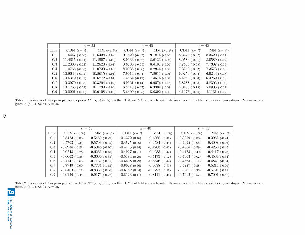
of a European put option with maturity T = 1 and strike K = 45 on the underlying S described in(5.11), at times s ∈ 0.1, 0.2, . . . , 0.9 and for α ∈ 35, 36, . . . , 45. We do not consider Europeanoption prices or deltas at time zero since they do not involve conditional expectations. Theestimation of the prices or deltas based on the CDM or MM approach includes the localisingtechnique. Each estimate results from the same set of N = 5 000 000 simulated paths. In Table1 we present the CDM and the MM estimates for the option prices for α ∈ 35, 40, 42. We alsoreport the relative errors in percentages to the Merton option prices, see paragraph 5.2.3. Similarresults were obtained for the other values of α ∈ 35, 36, . . . , 45. Table 2 shows the correspondingresults for the deltas. It turns out that the relative errors when comparing our approach to theapproach of [29] are very small. Hence the algorithm we developed is accurate.

25

α = 35 α = 40 α = 42time CDM (r.e. %) MM (r.e. %) CDM (r.e. %) MM (r.e. %) CDM (r.e. %) MM (r.e. %)

0.1 11.6447 ( 0.10) 11.6438 ( 0.09) 9.1820 (-0.02) 9.1816 (-0.03) 8.3520 ( 0.02) 8.3520 ( 0.01)

0.2 11.4615 (-0.04) 11.4597 (-0.05) 8.9133 (-0.07) 8.9133 (-0.07) 8.0584 ( 0.01) 8.0589 ( 0.02)

0.3 11.2838 ( 0.02) 11.2820 ( 0.01) 8.6180 (-0.05) 8.6181 (-0.05) 7.7308 ( 0.03) 7.7307 ( 0.03)

0.4 11.0765 (-0.03) 11.0730 (-0.06) 8.2936 ( 0.08) 8.2946 ( 0.09) 7.3569 ( 0.02) 7.3573 ( 0.03)

0.5 10.8633 ( 0.02) 10.8615 ( 0.01) 7.9014 (-0.04) 7.9011 (-0.04) 6.9254 (-0.02) 6.9243 (-0.03)

0.6 10.6319 ( 0.03) 10.6272 (-0.01) 7.4534 (-0.13) 7.4576 (-0.07) 6.4253 ( 0.00) 6.4269 ( 0.03)

0.7 10.3970 ( 0.05) 10.3894 (-0.02) 6.9561 ( 0.14) 6.9576 ( 0.16) 5.8288 ( 0.08) 5.8305 ( 0.10)

0.8 10.1765 ( 0.02) 10.1730 (-0.02) 6.3418 ( 0.07) 6.3398 ( 0.03) 5.0875 ( 0.15) 5.0906 ( 0.21)

0.9 10.0221 (-0.00) 10.0198 (-0.03) 5.6409 ( 0.05) 5.6392 ( 0.02) 4.1176 (-0.04) 4.1161 (-0.07)

Table 1: Estimates of European put option prices PEu(s, α) (5.12) via the CDM and MM approach, with relative errors to the Merton prices in percentages. Parameters aregiven in (5.11), we fix K = 45.

α = 35 α = 40 α = 42time CDM (r.e. %) MM (r.e. %) CDM (r.e. %) MM (r.e. %) CDM (r.e. %) MM (r.e. %)

0.1 -0.5473 ( 0.36) -0.5469 ( 0.29) -0.4372 (0.15) -0.4368 ( 0.03) -0.3959 (-0.36) -0.3955 (-0.44)

0.2 -0.5703 ( 0.35) -0.5703 ( 0.35) -0.4525 (0.06) -0.4534 ( 0.24) -0.4095 (-0.08) -0.4098 (-0.03)

0.3 -0.5936 (-0.21) -0.5943 (-0.10) -0.4715 (0.24) -0.4703 (-0.01) -0.4266 ( 0.59) -0.4260 ( 0.45)

0.4 -0.6243 (-0.28) -0.6233 (-0.45) -0.4927 (0.21) -0.4933 ( 0.33) -0.4423 ( 0.40) -0.4417 ( 0.26)

0.5 -0.6662 ( 0.38) -0.6660 ( 0.35) -0.5194 (0.29) -0.5173 (-0.12) -0.4603 (-0.02) -0.4588 (-0.34)

0.6 -0.7147 ( 0.65) -0.7137 ( 0.51) -0.5538 (0.29) -0.5546 ( 0.44) -0.4863 ( 0.11) -0.4841 (-0.34)

0.7 -0.7749 ( 0.90) -0.7766 ( 1.12) -0.6028 (0.36) -0.6038 ( 0.53) -0.5227 ( 0.28) -0.5211 (-0.01)

0.8 -0.8403 ( 0.11) -0.8355 (-0.46) -0.6782 (0.24) -0.6793 ( 0.40) -0.5801 ( 0.26) -0.5797 ( 0.19)

0.9 -0.9156 (-0.44) -0.9171 (-0.27) -0.8123 (0.11) -0.8141 ( 0.33) -0.7012 ( 0.57) -0.7006 ( 0.48)

Table 2: Estimates of European put option deltas ∆Eu(s, α) (5.13) via the CDM and MM approach, with relative errors to the Merton deltas in percentages. Parameters aregiven in (5.11), we fix K = 45.

26

5.3.2. Results for American option prices and deltasWe consider an American put option on the stock price process S with parameters given in

(5.11), the strike is fixed at K = 45. [1] and [22] developed a tree method to estimate theAmerican option price. In the current setting their estimate for the option price equals 9.954. TheMerton European option price at time zero equals 9.422. As mentioned before we approximatean American option by a Bermudan option using a time discretisation, we choose n = 10. Thedynamic programming algorithm presented in paragraph 5.1.2 and our representations are usedto estimate P (0, s0) and ∆(0, s0).

Figures 1-4 illustrate the influence of the variance reduction techniques on the estimates forthe price. The graphs on the right hand side are obtained by zooming in on the left graphs. ForN = 250i, i = 1, . . . , 30, we simulated N paths of the underlying at the discrete time points jT/n,j = 1, . . . , n, and we estimated the option price at time zero through the CDM and the MM, withand without control variable and with and without the optimal localisation technique. In case theEuropean option is included as a control variable, we put γ = 0.9.

The variance reduction techniques have a remarkable improvement on the results obtained viathe CDM and MM approaches. It appears that the CDM results show some more variation thanthe MM results.

Figure 1: Estimates for the American put option price obtained through the CDM and MM representations withoutcontrol variable and without localisation technique, against the number of simulated paths. In the right graph thevertical axis is restricted to [0, 100].

Figure 2: Estimates for the American put option price obtained through the CDM and MM representations withcontrol variable and without localisation technique, against the number of simulated paths. In the right graph thevertical axis is restricted to [8, 20].

27

Figure 3: Estimates for the American put option price obtained through the CDM and MM representations withoutcontrol variable and with localisation technique, against the number of simulated paths. In the right graph thevertical axis is restricted to [8, 20].

Figure 4: Estimates for the American put option price obtained through the CDM and MM representations withcontrol variable and with localisation technique, against the number of simulated paths. In the right graph thevertical axis is restricted to [9.5, 12].

Figure 5 presents the required time to estimate the American option price and delta at timezero through the backward dynamic programming algorithm combined with our Malliavin methodincluding a control variable and the optimal localising technique. The paths are simulated back-wards in time and the option prices and deltas are estimated simultaneously. The CPU time isgiven in terms of the number of simulated paths N , for discretisation parameter n ∈ 10, 20. Theconditional density method performs more or less at the same rate as the Malliavin method. TheCPU time is in the line of [4] and is quadratic in terms of the number of simulated paths. In [1]and [22] there is no clear indication about how long their algorithms take.

As described in paragraph 5.2.5 the computational effort is reduced when we consider anexponential localising function and perform a sorted algorithm. For example for n = 10 thismethod only needs 18 seconds for N = 10 000 and 41 seconds for N = 20 000.

Table 3 presents the estimated prices and deltas of the American put option with strikes30, 35, 40, 45, and 50, obtained through the sorted CDM and MM approach including the controlvariable and the exponential localisation function. For these estimates a time discretisation isperformed for n = 10 and 500 000 paths where simulated. We include the estimates for the pricesand deltas obtained by [1] and [22] respectively.

28

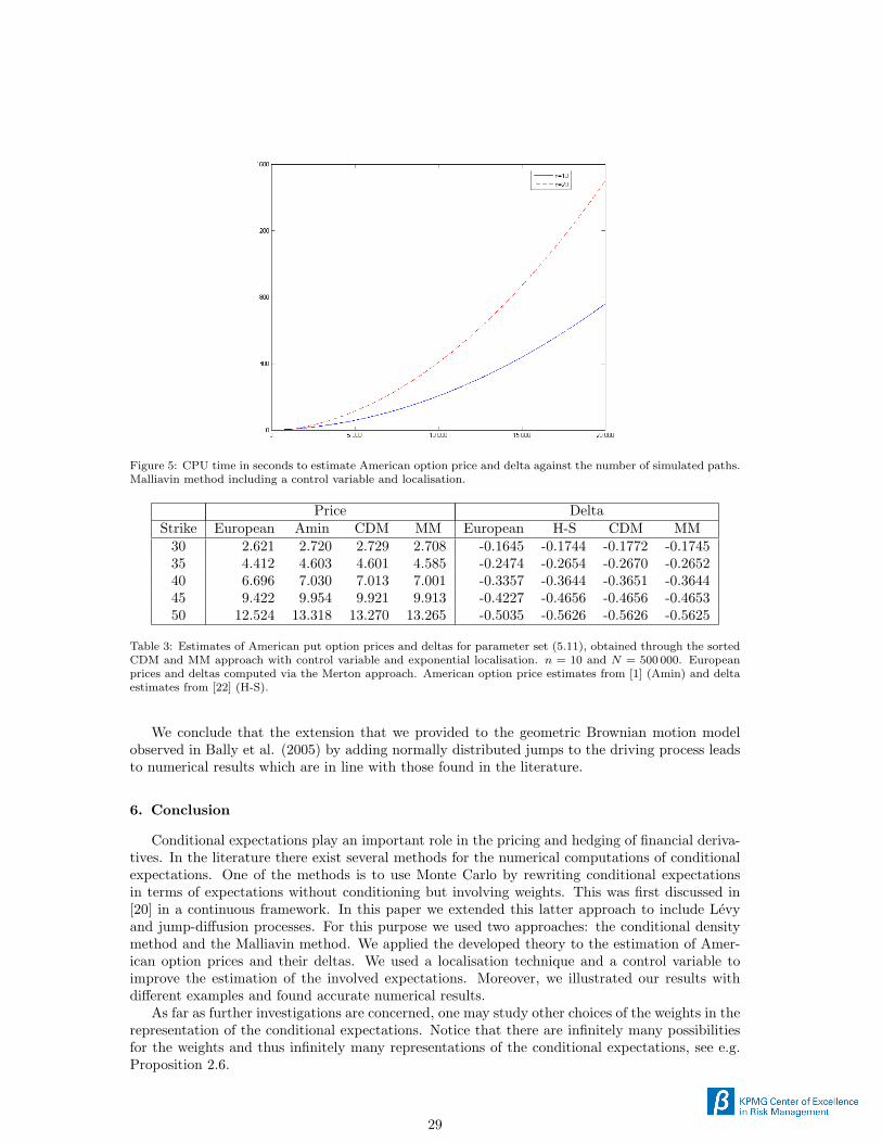
Figure 5: CPU time in seconds to estimate American option price and delta against the number of simulated paths.Malliavin method including a control variable and localisation.

Price DeltaStrike European Amin CDM MM European H-S CDM MM

30 2.621 2.720 2.729 2.708 -0.1645 -0.1744 -0.1772 -0.174535 4.412 4.603 4.601 4.585 -0.2474 -0.2654 -0.2670 -0.265240 6.696 7.030 7.013 7.001 -0.3357 -0.3644 -0.3651 -0.364445 9.422 9.954 9.921 9.913 -0.4227 -0.4656 -0.4656 -0.465350 12.524 13.318 13.270 13.265 -0.5035 -0.5626 -0.5626 -0.5625

Table 3: Estimates of American put option prices and deltas for parameter set (5.11), obtained through the sortedCDM and MM approach with control variable and exponential localisation. n = 10 and N = 500 000. Europeanprices and deltas computed via the Merton approach. American option price estimates from [1] (Amin) and deltaestimates from [22] (H-S).

We conclude that the extension that we provided to the geometric Brownian motion modelobserved in Bally et al. (2005) by adding normally distributed jumps to the driving process leadsto numerical results which are in line with those found in the literature.

6. Conclusion

Conditional expectations play an important role in the pricing and hedging of financial deriva-tives. In the literature there exist several methods for the numerical computations of conditionalexpectations. One of the methods is to use Monte Carlo by rewriting conditional expectationsin terms of expectations without conditioning but involving weights. This was first discussed in[20] in a continuous framework. In this paper we extended this latter approach to include Levyand jump-diffusion processes. For this purpose we used two approaches: the conditional densitymethod and the Malliavin method. We applied the developed theory to the estimation of Amer-ican option prices and their deltas. We used a localisation technique and a control variable toimprove the estimation of the involved expectations. Moreover, we illustrated our results withdifferent examples and found accurate numerical results.

As far as further investigations are concerned, one may study other choices of the weights in therepresentation of the conditional expectations. Notice that there are infinitely many possibilitiesfor the weights and thus infinitely many representations of the conditional expectations, see e.g.Proposition 2.6.

29

Appendix A. Malliavin Calculus

In this paper we make use of the Malliavin calculus as defined in [30]. The following propertiesand definitions concerning the Malliavin derivative in the direction of the Wiener process areapplied.

• The Malliavin derivative in the direction of the Brownian motion is denoted by D(0). Thespace D(0) contains all the random variables in L2(Ω) that are differentiable in the Wienerdirection.

• Chain ruleLet F ∈ D(0) and f be a continuously differentiable function with bounded derivative. Thenit holds that f(F ) ∈ D(0) and

D(0)f(F ) = f ′(F )D(0)F.

• Skorohod integral δ(0)

Let δ(0) be the adjoint operator of the directional derivative D(0). The operator δ(0) mapsL2(Ω× [0, T ]) to L2(Ω). The set of processes u ∈ L2(Ω× [0, T ]) such that∣∣∣E[ ∫ T

0

utD(0)t Fdt

]∣∣∣ ≤ C ‖F‖L2(Ω)

for all F ∈ D(0), is the domain of δ(0), denoted by Dom δ(0). For every u ∈ Dom δ(0) wedefine δ(0)(u) as the Skorohod integral in the Wiener direction of u by

E[Fδ(0)(u)] = E[∫ T

0

utD(0)t Fdt],

for any F ∈ D(0). The equation above is called the duality formula.

• Integration by partsLet Fu ∈ L2(Ω× [0, T ]), where F ∈ D(0), and u ∈ Dom δ(0). Then Fu ∈ Dom δ(0) and

δ(0)(Fu) = Fδ(0)(u)−∫ T

0

utD(0)t Fdt

if and only if the second part of the equation is in L2(Ω).

• Predictable processesLet u be a predictable process such that E[

∫ T0u2tdt] < ∞. Then u ∈ Dom δ(0) and the

Skorohod integral coincides with the Ito-integral

δ(0)(u) =∫ T

0

utdWt.

Acknowledgements The Financial support from the Agency for Innovation by Science and Technology

in Flanders (IWT) is gratefully acknowledged by Catherine Daveloose. Asma Khedher thanks the KPMG

Center of Excellence in Risk Management for the financial support. Part of the research by Asma Khedher

and Michele Vanmaele was carried out during their stay at the CAS - Centre of Advanced Study of the

Norwegian Academy of Science and Letter with the support from the research program SEFE. Michele

Vanmaele also acknowledges the Research Foundation Flanders (FWO) and the Special Research Fund

(BOF) of the Ghent University for providing the possibility to go on sabbatical leave to CAS.

30

References

[1] K.I. Amin. Jump diffusion option valuation in discrete time. The Journal of Finance, 48(5):1833–1863, 1993.

[2] J. Baldeaux. Quasi-Monte Carlo methods for the Kou model. Monte Carlo Methods andApplications, 14(4):281–302, 2008.

[3] V. Bally and G. Pages. Error analysis of the quantization algorithm for obstacle problems.Stochastic Processes and their Applications, 106:1–40, 2003.

[4] V. Bally, L. Caramellino, and A. Zanette. Pricing American options by Monte Carlo methodsusing a Malliavin calculus approach. Monte Carlo Methods and Applications, 11:97–133, 2005.

[5] O.E. Barndorff-Nielsen and N. Shephard. Modelling by Levy processes for financial economet-rics. In O.E. Barndorff-Nielsen, T. Mikosch, and S. Resnick, editors, Levy processes: Theoryand Applications. Birkhauser, Boston, 2001.

[6] O.E. Barndorff-Nielsen and N. Shephard. Econometric analysis of realized volatility and itsuse in estimating stochastic volatility models. Journal of the Royal Statistical Society: SeriesB (Statistical Methodology), 64:253–280, 2002.

[7] J. Barraquand and D. Martineau. Numerical valuation of high dimensional multivariateAmerican securities. Journal of Finance and Quantitative Analysis, 30:383–405, 1995.

[8] D. Bates. Jumps and stochastic volatility: exchange rate processes implicit in Deutsche Markoptions. Review of Financial Studies, 9(1):69–107, 1996.

[9] R. Bellman. Dynamic Programming. Princeton University Press, 1957.

[10] F.E. Benth, J. Kallsen, and T. Meyer-Brandis. A non-Gaussian Ornstein-Uhlenbeck processfor electricity spot price modeling and derivatives pricing. Applied Mathematical Finance, 14(2):153–169, 2007.

[11] F.E. Benth, G. Di Nunno, and A. Khedher. Levy models robustness and sensitivity. In QP-PQ: Quantum Probability and White Noise Analysis, Proceedings of the 29th Conference inHammamet, Tunisia, 1318 October 2008. H. Ouerdiane and A Barhoumi (eds.), 25:153–184,2010.

[12] F.E. Benth, G. Di Nunno, and A. Khedher. Robustness of option prices and their deltas inmarkets modelled by jump-diffusions. Communications on Stochastic Analysis, 5(2):285–307,2011.

[13] B. Bouchard and X. Warin. Monte-Carlo valuation of American options: Facts and newalgorithms to improve existing methods. Numerical Methods in Finance, Springer Proceedingsin Mathematics, 12:215–255, 2012.

[14] F. Bowman. Introduction to Bessel functions. Dover, 1958.

[15] D.W. Brewer, J.D. Tubbs, and O.E. Smith. A differential equations approach to the modallocation for a family of bivariate gamma distributions. Journal of Multivariate Analysis, 21(1):53–66, 1987.

[16] M. Broadie and P. Glasserman. Pricing American-style securities using simulation. Journalof Economic Dynamics and Control, 21(8-9):1323–1352, 1997.

[17] M.H.A. Davis and M.P. Johansson. Malliavin Monte Carlo Greeks for jump-diffusions.Stochastic Processes and their Applications, 116(1):101–129, 2006.

31

[18] G. Di Nunno, T. Meyer-Brandis, B. Øksendal, and F. Proske. Malliavin calculus and antici-pative Ito formulae for Levy processes. Infinite Dimensional Analysis, Quantum Probabilityand Related Topics, 8(2):235–258, 2005.

[19] E. Fournie, J.M. Lasry, J. Lebucheux, P.L. Lions, and N. Touzi. Applications of Malliavincalculus to Monte Carlo methods in finance. Finance and Stochastics, 3:391–412, 1999.

[20] E. Fournie, J.M. Lasry, J. Lebucheux, and P.L. Lions. Applications of Malliavin calculus toMonte Carlo methods in finance II. Finance and Stochastics, 5:201–236, 2001.

[21] P. Glasserman. Monte Carlo Methods in Financial Engineering. Springer, 2004.

[22] J. Hilliard and A. Schwartz. Pricing European and American derivatives under a jump-diffusion process: a bivariate tree approach. Journal of Financial and Quantitative Analysis,40(3), 2005.

[23] N. Ikeda and S. Watanabe. Stochastic Differential Equations and Diffusion Processes. ElsevierScience, 1981.

[24] I. Karatzas and S. Shreve. Brownian motion and stochastic calculus. Springer-Verlag, NewYork, 1991.

[25] A. Kohatsu-Higa and R. Pettersson. Variance reduction methods for simulation of densitieson Wiener space. SIAM Journal on Numerical Analysis, 40:431–450, 2002.

[26] S. Kou. A jump-diffusion model for option pricing. Management Science, 48:1086–1101, 2002.

[27] F.A. Longstaff and E.S. Schwarz. Valuing American options by simulations: a simple leastsquares approach. The Review of Financial Studies, 14:113–148, 2001.

[28] M. Martynov and O. Rozanova. On dependence of volatility on return for stochastic volatilitymodels. Stochastics: An International Journal of Probability and Stochastic Processes, 85(5):917–927, 2013.

[29] R.C. Merton. Option pricing when underlying stock returns are discontinuous. Journal ofFinancial Economics, 3:125–144, 1976.

[30] E. Petrou. Malliavin calculus in Levy spaces and applications to finance. Electronic Journalof Probability, 13:852–879, 2008.

[31] P. Protter. Stochastic integration and differential equations, Second Edition, Version 2.1.Number 21 in Stochastic Modelling and Applied Probability. Springer, Berlin, 2005.

[32] C.K. Raju. Products and compositions with the Dirac delta function. Journal of Physics A:Mathematical and General, 15(2):381–396, 1982.

[33] K.-I. Sato. Levy processes and infinitely divisible distributions. Number 68 in CambridgeStudies in Advanced Mathematics. Cambridge University Press, 1999.

[34] J.L. Sole, F. Utzet, and J. Vives. Canonical Levy process and Malliavin calculus. StochasticProcesses and their Applications, 117:165–187, 2007.

[35] A.W. van der Stoep, L.A. Grzelak, and C.W. Oosterlee. The Heston stochastic-local volatilitymodel: efficient Monte Carlo simulation. International Journal of Theoretical and AppliedFinance, 17(7), 2014.

32