tips, traps, and techniques in base sas for vertically
TRANSCRIPT

1
Paper 3161 – 2019
Tips, Traps, and Techniques in BASE SAS for vertically combining SAS data sets Jay Iyengar, Data Systems Consultants, Oak Brook, IL
ABSTRACT
Although not as frequent as merging, a data manipulation task which SAS programmers are required to perform is vertically combining SAS data sets. The SAS system provides multiple techniques for appending SAS data sets, which is otherwise known as concatenating, or stacking. There are pitfalls and adverse data quality consequences for using traditional approaches to appending data sets. There are also efficiency implications with using different methods to append SAS data files. In this paper, with practical examples, I examine the technical procedures that are necessary to follow to prepare data to be appended. I also compare different methods that are available in BASE SAS to append SAS data sets, based on efficiency criteria.
INTRODUCTION A SAS programmer may encounter different task situations on a given project where the need to append data sets arises. Some task examples involve the time period corresponding to the data files the programmer is using. A programmer may be provided monthly data sets and need to create an annual data set. Rather, a programmer may work with quarterly data sets and need to produce an annual data set. Also, a programmer may need to create a 3-year or 5-year data set from single-year data sets. In these examples, the purpose of appending is due to the need to analyze data over a longer time period, such as a full year, or to look at trends across a 3 or 5 year time span.
THE PROCESS OF APPENDING There are multiple ways of describing the process of vertically combining SAS datasets. Appending, concatenating, and stacking are all terms used which refer to vertically combining SAS data sets. The diagram in Figure 1 below visually illustrates the process of appending.
Figure 1. Append diagram flowchart

2
THE TRAPS OF DATA SET APPENDING SAS programmers are responsible for ensuring the validity of the data sources they use. Data quality issues arise when the data sets you need to append don’t have the same variable attributes. Data sets can have discrepancies in variable types, variable lengths, and variable formats. Another trap to lookout for is when the data sets don’t share the same set of variables.
DISCREPANCY IN VARIABLE TYPES; CHARACTER VS. NUMERIC In the case of variable type mismatches, SAS won’t append the data sets. The SAS log in Figure 2 shows error messages for a DATA STEP append corresponding to variable type mismatches.
62 Data Sales;
63 Set Sales_95
64 Sales_96;
ERROR: Variable Actual has been defined as both character and numeric. ERROR: Variable MonYr has been defined as both character and numeric. 65 Run;
NOTE: The SAS System stopped processing this step because of errors. WARNING: The data set WORK.SALES may be incomplete. When this step was stopped there were 0 observations and 11 variables.
Figure 2. Variable(s) is character in one data set, numeric in the other
DISCREPANCY IN VARIABLE LENGTHS When variables have different lengths, SAS will append the data sets. Though, the validity of the data may be compromised. This mainly pertains to character variables. An examination of the data might reveal truncated data values. The SAS log in figure 3 displays a warning message concerning a discrepancy in variable lengths. 62 Data NA_Sales;
63 Set US
64 Canada
65 Mexico;
66 Run;
WARNING: Multiple lengths were specified for the variable State by input data set(s). This can cause truncation of data. NOTE: There were 6336 observations read from the data set WORK.US. NOTE: There were 2880 observations read from the data set WORK.CANADA. NOTE: There were 2304 observations read from the data set WORK.MEXICO. NOTE: The data set WORK.NA_SALES has 11520 observations and 11 variables.
Figure 3. Data sets with length mismatch
DISCREPANCY IN VARIABLE FORMAT If there’s a difference in variable formats, SAS will also append the data sets. In this case, SAS will use the format from the first data set, regardless of how many data sets you’re appending. If you use PROC APPEND to concatenate, SAS will issue a warning message in the log about the format discrepancy. As the example in Figure 4 shows, SAS completes the append using the DATE7. format for sales_date, but issues a warning message describing the date format discrepancy.

3
90 Proc Append Base=Annual_Sales Data=QTR4;
91 Run;
NOTE: Appending WORK.QTR4 to WORK.ANNUAL_SALES. WARNING: Variable Sales_Date has format DATE7. on the BASE data set and format MMDDYY10. on the DATA data set. DATE7. used. NOTE: There were 2880 observations read from the data set WORK.QTR4. NOTE: 2880 observations added. NOTE: The data set WORK.ANNUAL_SALES has 11520 observations and 12 variables. NOTE: PROCEDURE APPEND used (Total process time): real time 0.00 seconds cpu time 0.00 seconds
Figure 4. Data set append with format discrepancy.
VARIABLE IN ONE DATA SET, NOT THE OTHER It’s entirely plausible that your data sets may include different sets of variables. In this case SAS will append the data, although it depends on the construct you use. However, SAS will assign missing values in the new data set for the records from the source data set which doesn’t have the variable. In the example in Figure 5, 12 monthly data sets are appended using the DATA STEP. The Jan and Feb data sets are missing both Product and Product_Type variables, respectively. In Appendix I, a sample of the Sales_Annual data set shows missing values for Product and Product_Type for Jan and Feb records.
62 Data Sales_Annual;
63 Set Jan
64 Feb
65 Mar
66 Apr
67 May
68 Jun
69 Jul
70 Aug
71 Sep
72 Oct
73 Nov
74 Dec;
75 Run;
NOTE: There were 960 observations read from the data set WORK.JAN. NOTE: There were 960 observations read from the data set WORK.FEB. NOTE: There were 960 observations read from the data set WORK.MAR. NOTE: There were 960 observations read from the data set WORK.APR. NOTE: There were 960 observations read from the data set WORK.MAY. NOTE: There were 960 observations read from the data set WORK.JUN. NOTE: There were 960 observations read from the data set WORK.JUL. NOTE: There were 960 observations read from the data set WORK.AUG. NOTE: There were 960 observations read from the data set WORK.SEP. NOTE: There were 960 observations read from the data set WORK.OCT. NOTE: There were 960 observations read from the data set WORK.NOV. NOTE: There were 960 observations read from the data set WORK.DEC. NOTE: The data set WORK.SALES_ANNUAL has 11520 observations and 11 variables. Figure 5. Monthly data set append using Data Step method.
4
BEST PRACTICES
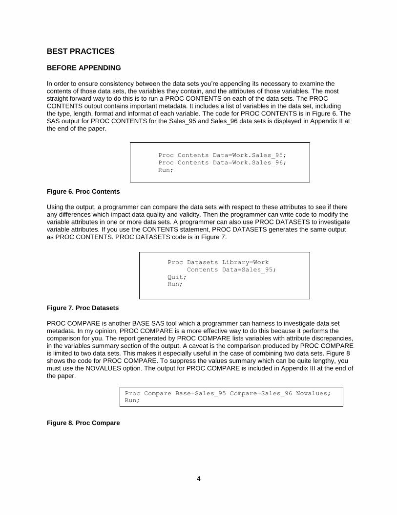
BEFORE APPENDING In order to ensure consistency between the data sets you’re appending its necessary to examine the contents of those data sets, the variables they contain, and the attributes of those variables. The most straight forward way to do this is to run a PROC CONTENTS on each of the data sets. The PROC CONTENTS output contains important metadata. It includes a list of variables in the data set, including the type, length, format and informat of each variable. The code for PROC CONTENTS is in Figure 6. The SAS output for PROC CONTENTS for the Sales_95 and Sales_96 data sets is displayed in Appendix II at the end of the paper.
Figure 6. Proc Contents
Using the output, a programmer can compare the data sets with respect to these attributes to see if there any differences which impact data quality and validity. Then the programmer can write code to modify the variable attributes in one or more data sets. A programmer can also use PROC DATASETS to investigate variable attributes. If you use the CONTENTS statement, PROC DATASETS generates the same output as PROC CONTENTS. PROC DATASETS code is in Figure 7. Figure 7. Proc Datasets
PROC COMPARE is another BASE SAS tool which a programmer can harness to investigate data set metadata. In my opinion, PROC COMPARE is a more effective way to do this because it performs the comparison for you. The report generated by PROC COMPARE lists variables with attribute discrepancies, in the variables summary section of the output. A caveat is the comparison produced by PROC COMPARE is limited to two data sets. This makes it especially useful in the case of combining two data sets. Figure 8 shows the code for PROC COMPARE. To suppress the values summary which can be quite lengthy, you must use the NOVALUES option. The output for PROC COMPARE is included in Appendix III at the end of the paper. Figure 8. Proc Compare
Proc Contents Data=Work.Sales_95;
Proc Contents Data=Work.Sales_96;
Run;
Proc Datasets Library=Work
Contents Data=Sales_95;
Quit;
Run;
Proc Compare Base=Sales_95 Compare=Sales_96 Novalues;
Run;

5
RESOLVING THE INCONSISTENCIES Once the data set differences have been discovered, the next logical step is to make changes to the data set variables to align them with each other. These variable modifications are easily performed using a DATA STEP to do simple data manipulations. For instance, you can increase the variable length using the LENGTH statement. The INPUT and PUT functions are handy to change variable type by explicitly converting variables from character to numeric and vice-versa. The RENAME and DROP option/statement can be harnessed to change variable names and drop extraneous variables. Figure 9 displays DATA STEP code which modifies variable attributes using these constructs. Data Sales_95;
Length State $22;
Set appsds.Sales_95
(Rename=(Mon=MonYR Quarter=Qtrc State=NewState Actual=Actualn)
Drop=County);
*Re-assign State with new length;
State = NewState;
*Convert Actual to numeric;
Actual = Input(Actualn, dollar12.2);
*Convert MonYR to character;
Quarter = Put(Qtrc, 3.);
Drop NewState Actualn Qtrc;
Run;
Figure 9. Data Step to correct attribute discrepancies
AFTER APPENDING Once the process of appending is complete, it’s important to verify variable attributes on the new data set. This only requires running a simple PROC CONTENTS on the output data set. For many appends the attributes from the first data set prevail. However, it’s useful to examine the descriptor portion of the data set to ensure that the results conform to expectations. I recommend running PROC CONTENTS on the new data set after the append executes. The code for PROC CONTENTS was displayed earlier in this paper in Figure 6. A diligent SAS programmer reviews the data values to ensure the quality and accuracy of the data set. As described, the process of the append may truncate values for variables that have length discrepancies. Also in the new data set, missing values will be assigned for records from a data set without a corresponding variable. PROC FREQ is a good data validity tool for checking character data values. With PROC FREQ, you can output frequency tables on each variable in the data set. The code for PROC FREQ is displayed in Figure 10 below.
Figure 10. Proc Freq
It’s a good practice to document the values that constitute a variable before combining data sets. Thus, I also recommend running frequency tables on input data sets prior to executing the append.
Proc Freq Data=Sales_95;
Tables State Quarter / List Missing;
Run;

6
METHODS OF APPENDING
DATA STEP SET STATEMENT I consider the DATA STEP SET statement to be the traditional approach to appending data sets. When I first started programming in SAS, I only used the DATA STEP to append data sets. This is probably because it was the first method I learned, and I hadn’t learned the other techniques. To concatenate two data sets together using the SET statement, a user simply specifies SAS data sets one after the other. Using the DATA STEP SET statement, an unlimited number of data sets can be appended together. I’ve used the DATA STEP to append up to 12 SAS data sets. A SAS code example of DATA STEP concatenation is in Figure 11.
Figure 11. Data Step Concatenation
OBSTACLES TO APPENDING In using the conventional DATA STEP method, SAS will generally append data sets together which have attribute differences. In the case of variables which have discrepancies in type (character vs. numeric), SAS will not append the data sets together and will issue an explicit error message detailing the discrepancy. In the three other cases of discrepancies, SAS will append the data sets and will issue a warning message when there’s a length discrepancy. For Length and Format discrepancies, SAS will use the attributes from the first data set for the new variable on the appended data set. However, when one input data set is missing a variable, SAS will write missing values for those records from the data set. Figure 12 below details the results for each case of variable discrepancies when using the DATA STEP Set statement.
Discrepancy Result Note
Variable Type Will not Append Error Message
Variable Length Will Append Variable length in first data set carried over. Issues Warning Message
Variable Format Will Append Variable format from first data set carried over.
Variables Will Append
Missing values for records from data set without variable
Figure 12. Data Step Set statement – data set discrepancies
EFFICIENCY IMPLICATIONS The DATA STEP can be a time-consuming and resource intensive construct. Using the DATA STEP usually means a sequential reading of observations in the input data sets. Using the DATA STEP method, all data sets listed in the SET statement are read and processed. In DATA STEP mechanics, this means that all observations are loaded to the program data vector and written to the new output data set. Reading and writing large volumes of data results in extensive consumption of input/output (I/O) resources. Thus, using the DATA STEP has the drawback of inefficiency by consuming I/O resources. It can also entail substantial CPU or processing time.
Data Sales;
Set Sales_95
Sales_96;
Run;

7
The effect on efficiency is positively correlated with the amount of data being processed. If you are appending large data sets which contain millions of records, the effect on efficiency will be proportionately large. You should expect a relative increase in time to process an append which requires substantial I/O and other resources, due to the large amount of data being processed. Figure 13 displays a concatenation example. The notes in the SAS log confirm the full set of observations from each data set were read using the DATA STEP.
74 Data NDF_DSC;
75 Set NDF_1994
76 NDF_1995_AFTER;
77 Run;
NOTE: There were 515155 observations read from the data set WORK.NDF_1994. NOTE: There were 533420 observations read from the data set WORK.NDF_1995_AFTER. NOTE: The data set WORK.NDF_DSC has 1048575 observations and 36 variables. NOTE: DATA statement used (Total process time): real time 50.36 seconds cpu time 5.44 seconds Figure 13. Data Step Concatenation example
PROC APPEND Another BASE SAS construct that can be used to append SAS data sets is the APPEND procedure. With PROC APPEND, you specify a BASE data set, and a DATA data set. PROC APPEND has the limitation of combining only two data sets. The coding of PROC APPEND is straight forward. Unlike the DATA STEP, it’s not necessary to specify a new output data set. The BASE data set becomes the new data set with records appended from the DATA data set. An example of PROC APPEND is in Figure 14.
106 Proc Append Base=US Data=Canada_Mexico;
107 Run;
NOTE: Appending WORK.CANADA_MEXICO to WORK.US. WARNING: Variable Actual has format COMMA12. on the BASE data set and format DOLLAR12. on the DATA data set. COMMA12. used. WARNING: Variable Predict has format COMMA12. on the BASE data set and format DOLLAR12. on the DATA data set. COMMA12. used. WARNING: Variable Mon was not found on BASE file. The variable will not be added to the BASE file. WARNING: Variable State has different lengths on BASE and DATA files (BASE 10 DATA 22). ERROR: No appending done because of anomalies listed above. Use FORCE option to append these files. NOTE: 0 observations added. NOTE: The data set WORK.US has 6336 observations and 10 variables. NOTE: Statements not processed because of errors noted above. Figure 14. Proc Append - SAS log
By default, PROC APPEND will not combine the data sets if discrepancies exist between dataset variables, with the exception of format discrepancies. As figure 14 shows, PROC APPEND will issue explicit warning messages if discrepancies exist in variables or variable attributes. The messages state the specific discrepancy, and the variables involved on the BASE and DATA data sets respectively.

8
THE FORCE OPTION Using the FORCE option, PROC APPEND will combine data sets if discrepancies exist in the variable type, length, or variables between the BASE and DATA data sets. SAS data sets that have a discrepancy in formats will be appended without using FORCE. When there’s a discrepancy in variable attributes between BASE and DATA data sets, the attributes from the BASE data set prevail. The table in figure 15 shows the result and details for various attribute differences.
Trap Result Note
Variable Type Will append with FORCE option. Issues warning message.
Missing values for records from DATA data set.
Variable Length Will append with FORCE option. Issues warning message.
Length from BASE data set prevails. Records from DATA data set may contain truncated values.
Variable Format Will append w/warning msg. Format from BASE data set prevails.
Variables Will Append with FORCE option. Issues warning message.
Missing values for records from data set without variable
Figure 15. Proc Append – data set discrepancies
In figure 16 is an example using PROC APPEND with the FORCE option in the SAS log. The input data sets have a mismatch in type for the ACTUAL variable, but the append still completes. 73 Proc Append Base=Sales_95 Data=Sales_96 Force;
74 Run;
NOTE: Appending WORK.SALES_96 to WORK.SALES_95. WARNING: Variable Actual not appended because of type mismatch. NOTE: FORCE is specified, so dropping/truncating will occur. NOTE: There were 5760 observations read from the data set WORK.SALES_96. NOTE: 5760 observations added. NOTE: The data set WORK.SALES_95 has 11520 observations and 11 variables. NOTE: PROCEDURE APPEND used (Total process time): real time 0.00 seconds cpu time 0.01 seconds Figure 16. Proc Append with FORCE option.
EFFICIENCY IMPLICATIONS The main advantage of using PROC APPEND is improved processing efficiency. Unlike the DATA STEP method, using PROC APPEND only the DATA data set is read and processed. The records from the DATA data set are simply added to the end of the BASE data set. This results in improved processing efficiency over the DATA STEP method, especially if the BASE data set is large. The better processing efficiency with PROC APPEND entails savings of valuable computing resources, such as I/O. In Figure 17 is an example using PROC APPEND. The notes in the SAS log explain that the full set of observations in the DATA data set were read and added.

9
74 Proc Append Base=NDF_1994 Data=NDF_1995_AFTER;
75 Run;
NOTE: Appending WORK.NDF_1995_AFTER to WORK.NDF_1994. NOTE: There were 533420 observations read from the data set WORK.NDF_1995_AFTER. NOTE: 533420 observations added. NOTE: The data set WORK.NDF_1994 has 1048575 observations and 36 variables. NOTE: PROCEDURE APPEND used (Total process time): real time 27.33 seconds cpu time 2.80 seconds Figure 17. Proc Append efficiency example.
PROC SQL SET OPERATORS PROC SQL has capabilities which extend to appending SAS data sets. You can vertically combine SAS data sets with PROC SQL using SET operators. There are four different SET operators in PROC SQL; INTERSECT, EXCEPT, UNION, and OUTER UNION. The set operator which appends data sets and is equivalent to the DATA STEP SET statement and PROC APPEND is OUTER UNION. Each of the four SET operators selects records to include in the result set, and combine data sets in one manner or another. The INTERSECT operator selects records which are common to both tables. The EXCEPT operator selects records in the first table that are not in the second table. The UNION operator selects records that are exclusive to each of the tables, and records that are common to the tables. The OUTER UNION operator selects all records from both tables. By default, the first three SET operators select unique records from both tables. To select both unique and duplicate records, you need to use the ALL keyword. Since OUTER UNION selects all records by default, use of the ALL keyword isn’t necessary. However, unlike the other three operators, OUTER UNION doesn’t append or overlay columns by default. To append columns according to column name, use of the CORR keyword is required.
Figure 18 is a SAS log which displays an append using the PROC SQL OUTER UNION set operator. 74 Proc Sql;
75 Create Table NDF_PSQL as
76 Select *
77 From NDF_1994
78 Outer Union Corr
79 Select *
80 From NDF_1995_AFTER;
NOTE: Table WORK.NDF_PSQL created, with 1048575 rows and 36 columns. 81 Quit;
NOTE: PROCEDURE SQL used (Total process time): real time 48.91 seconds cpu time 8.00 seconds Figure 18. Outer Union Set operator
The PROC SQL OUTER UNION construct has the capability of appending more than two SAS data sets. In comparison PROC APPEND is limited to two tables. To perform this with PROC SQL set operators, you need to combine more than two SELECT queries. With this method each additional table combined requires a separate query.

10
With PROC SQL OUTER UNION, more lines of code are required than a DATA STEP append because of having to repeat SELECT and OUTER UNION CORR for each extra input table. The DATA STEP also permits appending more than two input tables. The efficiency impact of PROC SQL OUTER UNION is similar to the DATA STEP SET statement. The PROC SQL example in figure 18 took 48.91 seconds of real time to execute. If we examine the results from Figure 13, SAS took 50.36 seconds of real time to execute the append using the DATA STEP SET statement. Using PROC SQL OUTER UNION shows only a minor increase in performance of about 1.5 seconds.
PROC DATASETS Another construct in BASE SAS which can be used to append data sets is PROC DATASETS. With PROC DATASETS, you use the APPEND statement to concatenate. The construct is quite similar to PROC APPEND. The user specifies a BASE and a DATA data set. If there discrepancies in variable attributes between data sets, the BASE data set attributes prevail. PROC DATASETS also has a FORCE option which can be used to execute the append if data set differences exist in variables, variable length or formats. Figure 19 is a SAS log with a PROC DATASETS append example. 73 Proc Datasets Library=Work nolist;
74 Append Base=NDF_1994 Data=NDF_1995_AFTER;
75 Run;
NOTE: Appending WORK.NDF_1995_AFTER to WORK.NDF_1994. NOTE: There were 533420 observations read from the data set WORK.NDF_1995_AFTER. NOTE: 533420 observations added. NOTE: The data set WORK.NDF_1994 has 1048575 observations and 36 variables. 76 Quit;
NOTE: PROCEDURE DATASETS used (Total process time): real time 22.85 seconds cpu time 2.74 seconds Figure 19. Proc Datasets Append statement
The efficiency implications of using PROC DATASETS are also the same as PROC APPEND. The example in figure 19 shows the observations from the DATA data set (NDF_1995_AFTER) were read and added to the end of the BASE data set (NDF_1994). As evidenced with PROC DATASETS, SAS only reads the DATA data set when appending data sets. If you look at the processing time in the examples, PROC DATASETS took about 5 seconds less real time (22.85) than PROC APPEND (27.33). The only real difference between PROC APPEND and the PROC DATASETS APPEND statement is the default SAS library. PROC APPEND uses WORK or USER as its default library, and with PROC DATASETS the default library is the procedure input library. The remaining aspects, including the structure of the append and the append processing, are the same.
11
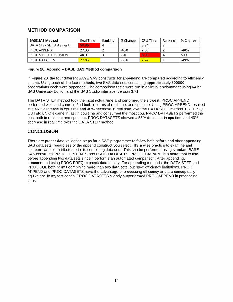
METHOD COMPARISON
BASE SAS Method Real Time Ranking % Change CPU Time Ranking % Change
DATA STEP SET statement 50.36 4 5.34 3
PROC APPEND 27.33 2 -46% 2.80 2 -48%
PROC SQL OUTER UNION 48.91 3 -3% 8.00 4 50%
PROC DATASETS 22.85 1 -55% 2.74 1 -49%
Figure 20. Append – BASE SAS Method comparison
In Figure 20, the four different BASE SAS constructs for appending are compared according to efficiency criteria. Using each of the four methods, two SAS data sets containing approximately 500000 observations each were appended. The comparison tests were run in a virtual environment using 64-bit SAS University Edition and the SAS Studio interface, version 3.71 The DATA STEP method took the most actual time and performed the slowest. PROC APPEND performed well, and came in 2nd both in terms of real time, and cpu time. Using PROC APPEND resulted in a 46% decrease in cpu time and 48% decrease in real time, over the DATA STEP method. PROC SQL OUTER UNION came in last in cpu time and consumed the most cpu. PROC DATASETS performed the best both in real time and cpu time. PROC DATASETS showed a 55% decrease in cpu time and 49% decrease in real time over the DATA STEP method.
CONCLUSION There are proper data validation steps for a SAS programmer to follow both before and after appending SAS data sets, regardless of the append construct you select. It’s a wise practice to examine and compare variable attributes prior to combining data sets. This can be performed using standard BASE SAS constructs PROC CONTENTS and PROC DATASETS. PROC COMPARE is a better tool to use before appending two data sets since it performs an automated comparison. After appending, I recommend using PROC FREQ to check data quality. For appending methods, the DATA STEP and PROC SQL both permit combining more than two data sets, but have efficiency limitations. PROC APPEND and PROC DATASETS have the advantage of processing efficiency and are conceptually equivalent. In my test cases, PROC DATASETS slightly outperformed PROC APPEND in processing time.

12
REFERENCES
SAS Institute Inc., 2010. SAS Certification Prep Guide – Advanced Programming for SAS 9. Cary, NC:
SAS Institute Inc. ACL. “Using ACL Analytics>Preparing data for Analysis>Combining Data”. Accessed August 9, 2018. https://enablement.acl.com/helpdocs/analytics/13/user-guide/en-us/ Content/ da_cmbining_data/ combining_data.htm?TocPath=Combining%20data|_____0
ACKNOWLEGEMENTS The author would like to thank MaryAnne DePesquo, SAS Global Forum 2019 Conference Chair, and the SAS Global Forum 2019 Executive Committee and Conference Team for accepting my abstract and paper, and organizing a great conference. Jay Iyengar is Principal of Data Systems Consultants LLC. He is a SAS Consultant, Trainer, and SAS Certified Advanced Programmer. He is co-leader of the Chicago SAS Users Group, WCSUG. He’s presented papers at SAS Global Forum (SGF), Midwest SAS Users Group (MWSUG), Wisconsin Illinois SAS Users Group (WIILSU), Northeast SAS Users Group (NESUG), and Southeast SAS Users Group (SESUG) conferences. He has been using SAS since 1997. His industry experience includes Healthcare, Pharmaceutical, Public Health, Direct Marketing and Educational Testing.
CONTACT INFORMATION Your comments and questions are valued and encouraged. Contact the author at: Jay Iyengar Data Systems Consultants LLC Oak Brook, IL 60523 Email: [email protected] Linkedin: https://www.linkedin.com/in/jisasprogconsult
TRADEMARK CITATION SAS and all other SAS Institute Inc. product or service names are registered trademarks or trademarks of SAS Institute Inc. in the USA and other countries. ® indicates USA registration. Other brand and product names are registered trademarks or trademarks of their respective companies.

13
APPENDIX I
Country State County Actual Predict ProductType Year Quarter Mon MonYr Product
Canada Saskatchewan
$540.00 $1,301.60 BED 1996 1 Jan Jan-96
Canada Saskatchewan
$101.60 $547.20 CHAIR 1996 1 Jan Jan-96
Canada Saskatchewan
$1,163.20 $588.00 DESK 1996 1 Jan Jan-96
Canada Saskatchewan
$1,070.40 $248.00 SOFA 1996 1 Jan Jan-96
Canada Saskatchewan
$35.20 $392.00 BED 1996 1 Jan Jan-96
Canada Saskatchewan
$931.20 $1,158.40 CHAIR 1996 1 Jan Jan-96
Canada Saskatchewan
$816.00 $996.80 DESK 1996 1 Jan Jan-96
U.S.A. California
$1,782.96 $568.48
1995 1 Feb Feb-95 FURNITURE
U.S.A. California
$2,014.16 $2,358.24
1995 1 Feb Feb-95 FURNITURE
U.S.A. California
$2,151.52 $1,025.44
1995 1 Feb Feb-95 OFFICE
U.S.A. California
$2,584.00 $2,132.48
1995 1 Feb Feb-95 OFFICE
U.S.A. California
$1,856.40 $1,308.32
1995 1 Feb Feb-95 FURNITURE
U.S.A. California
$897.60 $2,759.44
1995 1 Feb Feb-95 FURNITURE

14
APPENDIX II
Data Set Name APPSDS.SALES_95 Observations 576
0
Member Type DATA Variables 11
Engine V9 Indexes 0
Created 05/18/2018 14:04:12 Observation Length 120
Last Modified 05/18/2018 14:04:12 Deleted Observations 0
Protection Compressed NO
Data Set Type Sorted NO
Label
Data Representation SOLARIS_X86_64, LINUX_X86_64, ALPHA_TRU64,
LINUX_IA64
Encoding utf-8 Unicode (UTF-8)
Engine/Host Dependent Information
Data Set Page Size 65536
Number of Data Set Pages 11
First Data Page 1
Max Obs per Page 545
Obs in First Data Page 518
Number of Data Set Repairs 0
Filename /folders/myfolders/SAS Data
Sets/Appending_sds/sales_95.sas7bdat
Release Created 9.0401M4
Host Created Linux
Inode Number 139145
Access Permission rw-rw-r--
Owner Name Sasdemo
File Size 768KB
File Size (bytes) 786432

15
Alphabetic List of Variables and Attributes
# Variable Type Len Format Informat
4 Actual Num 8 DOLLAR12.2 DOLLAR12.2
1 Country Char 10 $10. $10.
3 County Char 20 $20. $20.
10 Mon Char 3 $3. $3.
11 MonYr Num 8 MONYY. MONYY.
5 Predict Num 8 DOLLAR12.2 DOLLAR12.2
6 Product Char 10 $10. $10.
7 ProductType Char 10 $10. $10.
9 Quarter Num 8 2. 2.
2 State Char 22 $22. $22.
8 Year Num 8 4. 4.

16
Data Set Name APPSDS.SALES_96 Observations 576
0
Member Type DATA Variables 11
Engine V9 Indexes 0
Created 05/21/2018 15:31:14 Observation Length 120
Last Modified 05/21/2018 15:31:14 Deleted Observations 0
Protection Compressed NO
Data Set Type Sorted NO
Label
Data Representation SOLARIS_X86_64, LINUX_X86_64, ALPHA_TRU64,
LINUX_IA64
Encoding utf-8 Unicode (UTF-8)
Engine/Host Dependent Information
Data Set Page Size 65536
Number of Data Set Pages 11
First Data Page 1
Max Obs per Page 545
Obs in First Data Page 518
Number of Data Set Repairs 0
Filename /folders/myfolders/SAS Data
Sets/Appending_sds/sales_96.sas7bdat
Release Created 9.0401M4
Host Created Linux
Inode Number 139230
Access Permission rw-rw-r--
Owner Name Sasdemo
File Size 768KB
File Size (bytes) 786432

17
Alphabetic List of Variables and Attributes
# Variable Type Len Format Informat
4 Actual Num 8 DOLLAR12.2 DOLLAR12.2
1 Country Char 10 $10. $10.
3 County Char 20 $20. $20.
10 Mon Char 3 $3. $3.
11 MonYr Num 8 MONYY. MONYY.
5 Predict Num 8 DOLLAR12.2 DOLLAR12.2
6 Product Char 10 $10. $10.
7 ProductType Char 10 $10. $10.
9 Quarter Num 8 2. 2.
2 State Char 22 $22. $22.
8 Year Num 8 4. 4.

18
APPENDIX III
The COMPARE Procedure
Comparison of WORK.US with WORK.CANADA
(Method=EXACT)
Data Set Summary
Dataset Created Modified NVar NObs
WORK.US 11JUN18:22:05:40 11JUN18:22:05:40 10 6336
WORK.CANADA 11JUN18:21:57:27 11JUN18:21:57:27 11 2880
Variables Summary
Number of Variables in Common: 10.
Number of Variables in WORK.CANADA but not in WORK.US: 1
Number of Variables with Differing Attributes: 2.
Listing of Common Variables with Differing Attributes
Variable Dataset Type Length Format Informat
State WORK.US Char 10
WORK.CANADA Char 22 $22. $22.
MonYR WORK.US Num 8 MONYY7.
WORK.CANADA Num 8 MONYY. MONYY.