DI

SC

US

SI

ON

P

AP

ER

S

ER

IE

S

Forschungsinstitut zur Zukunft der ArbeitInstitute for the Study of Labor

Tipping and Residential Segregation: A Unifi ed Schelling Model

IZA DP No. 4413

September 2009

Junfu Zhang

Tipping and Residential Segregation:

A Unified Schelling Model

Junfu Zhang Clark University

and IZA

Discussion Paper No. 4413 September 2009

IZA

P.O. Box 7240 53072 Bonn

Germany

Phone: +49-228-3894-0 Fax: +49-228-3894-180

E-mail: iza@iza.org

Any opinions expressed here are those of the author(s) and not those of IZA. Research published in this series may include views on policy, but the institute itself takes no institutional policy positions. The Institute for the Study of Labor (IZA) in Bonn is a local and virtual international research center and a place of communication between science, politics and business. IZA is an independent nonprofit organization supported by Deutsche Post Foundation. The center is associated with the University of Bonn and offers a stimulating research environment through its international network, workshops and conferences, data service, project support, research visits and doctoral program. IZA engages in (i) original and internationally competitive research in all fields of labor economics, (ii) development of policy concepts, and (iii) dissemination of research results and concepts to the interested public. IZA Discussion Papers often represent preliminary work and are circulated to encourage discussion. Citation of such a paper should account for its provisional character. A revised version may be available directly from the author.

IZA Discussion Paper No. 4413 September 2009

ABSTRACT

Tipping and Residential Segregation: A Unified Schelling Model*

This paper presents a Schelling-type checkerboard model of residential segregation formulated as a spatial game. It shows that although every agent prefers to live in a mixed-race neighborhood, complete segregation is observed almost all of the time. A concept of tipping is rigorously defined, which is crucial for understanding the dynamics of segregation. Complete segregation emerges and persists in the checkerboard model precisely because tipping is less likely to occur to such residential patterns. Agent-based simulations are used to illustrate how an integrated residential area is tipped into complete segregation and why this process is irreversible. This model incorporates insights from Schelling’s two classical models of segregation (the checkerboard model and the neighborhood tipping model) and puts them on a rigorous footing. It helps us better understand the persistence of residential segregation in urban America. JEL Classification: C72, C73, D62, R13 Keywords: residential segregation, tipping, checkerboard model Corresponding author: Junfu Zhang Department of Economics Clark University 950 Main Street Worcester, MA 01610 USA E-mail: juzhang@clarku.edu

* This paper has benefited from comments by Alex Anas, Richard Arnott, Robert Axtell, Robert Helsley, Amy Ickowitz, Robert McMillan, Juan Robalino, Steve Ross, Harris Selod, Peyton Young, several anonymous referees, and seminar or conference participants at Boston College, Clark University, Northeastern University, SHUFE, WPI, the ESHIA Conference at George Mason University, the Econometric Society Summer Meetings at Duke, the Workshop on Residential Sprawl and Segregation in Dijon, France, the Third World Congress of the Game Theory Society at Northwestern University, and the ASSA Meetings in San Francisco.

1. Introduction

For three decades, survey data have consistently shown that African Americans prefer to

live in integrated neighborhoods with half blacks or a slight black majority.1 For example, in

1982, the General Social Surveys asked black respondents about their most preferred

neighborhood racial composition and found that 61.6 percent of them picked “half black, half

white” as the top choice (Davis and Smith, 1993). Data collected in a Multi-City Study of Urban

Inequality (MCSUI) during the 1990s also showed that 50 percent of black interviewees chose a

50-50 neighborhood as the most attractive and 99 percent of them indicated a willingness to move

into such neighborhoods (Krysian and Farley, 2002).

Survey results also demonstrated that whites, although generally less enthusiastic about

50-50 type neighborhoods than blacks, have increasingly endorsed the idea of residential

integration (Schuman et al., 1997). The same MCSUI data indicated that 60 percent of whites felt

comfortable with neighborhoods with one-third blacks and that 45 percent of whites were willing

to move into such neighborhoods (Charles, 2003).

These stated preferences are in stark contrast with the high levels of racial housing

segregation in reality. Using the 1990 Census data, Massey and Denton (1993) find that

residential segregation between blacks and whites remains a striking feature of many U.S.

metropolitan areas, a situation they describe as the “American apartheid.” According to the same

Census data, very few blacks actually live in “half black, half white” neighborhoods, in contrast

to the survey results cited above (Zhang, 2004a).2 The latest 2000 Census data show only modest

steps toward integration (see, e.g., Glaeser and Vigdor, 2001; Logan et al., 2004).3

1 See, e.g., Farley et al. (1978), Farley et al. (1994), Farley et al. (1997), Krysan and Farley (2002), Schuman et al. (1997), and Bobo and Zubrinsky (1996). 2 For example, only 2.91 percent of blacks in Chicago, 2.97 percent in Cleveland, and 2.56 percent in Detroit live in “half black, half white” neighborhoods, which Zhang (2004a) broadly defines as any neighborhood with 40-60 percent blacks. 3 In terms of long-term trend, the absolute degree of residential segregation peaked in 1970 and has been declining since (Cutler et al., 1999; Glaeser and Vigdor, 2001). However, the decline is too small relative to the dramatic change in racial attitudes, federal housing policy, and the socioeconomic status of blacks.

1

This persistence of residential segregation in urban America is generally considered a

social problem because it has adverse effects, especially on blacks. Kain (1968) has long argued

that residential segregation leads to a “spatial mismatch” between blacks and their potential

employers that diminishes blacks’ employment opportunities. Wilson (1987) echoes this point in

a highly influential study of the “truly disadvantaged” inner city underclass in America. Massey

and Denton (1993) argue that segregation is at the root of many problems facing blacks.

Numerous studies have since documented that residential segregation is associated with negative

outcomes for blacks in terms of academic performance, educational attainment, employment,

single parenthood, poverty, criminal behaviors, and even health outcomes (see, e.g., Card and

Rothstein, 2007; Cutler and Glaeser, 1997; Galster, 1987; Orfield and Eaton, 1996; Shihadeh and

Flynn, 1996; Williams and Collins, 2001).4

There are three primary explanations for the persistence of segregation.5 The first is

derived from a long-standing hypothesis that physical distance between racial groups reflects

their social distance. This explanation holds that segregation persists because lower-income

blacks cannot afford to move to white neighborhoods although they would like to (Clark and

Ware, 1997; Cloutier, 1982; Iceland and Wilkes, 2006; Marshall and Jiobu, 1975).6 The second

explanation emphasizes various forms of racial discrimination in the housing market. It argues

The inconsistency between the small steps toward integration and the widely expressed racial tolerance is particularly puzzling. As Farley and Frey (1994) observed, there is “a gap between attitude and behavior.” 4 To what extent these negative effects are causal is still debatable. For example, evidence from a recent randomized policy experiment (HUD’s Moving to Opportunity program) shows that moving out of high-poverty neighborhoods has limited positive effects on minority families. See Kling et al. (2007) and many of the evaluation studies they cite. See also Ludwig et al. (2008) and Clampet-Lundquist and Massey (2008) for a debate on the validity of evidence from the experiment. 5 Dawkins (2004) points out a fourth possible explanation of the persistence of segregation that stresses on the information asymmetry in the housing market. More specifically, if information on housing mostly comes from local sources, then blacks living in predominantly black neighborhoods would have very limited information about the availability and costs of housing in predominantly white neighborhoods. This lack of information may prevent them from moving across the color line. This hypothesis, though equally plausible, has been under-researched. 6 This hypothesis has always been challenged because empirical evidence has consistently shown that high levels of segregation exist in every socioeconomic group (see, e.g., Taeuber, 1968; Farley, 1995; Darden and Kamel, 2000; and Zhang, 2003). Bayer et al. (2004) find that socioeconomic factors explain only a small proportion of the segregation of blacks although they can explain a large proportion of the segregation of Hispanics.

2

that discriminatory behaviors of real estate agents, mortgage lenders, and insurance providers

prevent blacks from moving into their most preferred neighborhoods (see, e.g., Goering and

Wienk, 1996; Yinger, 1986, 1995). The third explanation points to the fact that whites have less

favorable feelings toward integrated neighborhoods than blacks. It contends that there are not

enough whites willing to reside in neighborhoods with 50 percent or more blacks (Emerson et al.,

2001; Krysian and Farley, 2002; Vigdor, 2003).7 Given these explanations for the persistence of

segregation, one naturally expects that residential integration will occur as long as socioeconomic

inequalities between blacks and whites continue to narrow, whites’ attitudes toward integrated

neighborhoods continue to become more favorable, and anti-discrimination laws are more

stringently enforced.8

In this paper, I show that the prospect of residential integration may be bleaker than what

is generally perceived. I present a rigorous model that incorporates important insights from

Thomas Schelling’s two models of segregation (Schelling, 1969, 1971, 1972, and 1978). I will

show that residential segregation could emerge and persist even if the following three conditions

hold simultaneously: (1) There exists no racial discrimination of any type; (2) both blacks and

whites prefer to live in 50-50 neighborhoods; and (3) the socioeconomic disparities between

blacks and whites are completely eliminated.

This paper makes two contributions. First, it offers an explanation for the persistence of

residential segregation in U.S. metropolitan areas observed in the past two decades. Existing

studies on the persistence of segregation generally assume that if integration is a preferred

7 These three explanations are not necessarily mutually exclusive. For example, Sethi and Somanathan (2004) explain residential segregation based on a preference over both neighborhood affluence and its racial composition. Their model suggests that under certain conditions a narrowing racial income gap may increase rather than decrease the levels of segregation. 8 In fact, there is evidence for the changing attitudes of whites. Survey data show that more and more whites tend to agree with the principle that blacks should be able to live wherever they can afford and that more and more whites tend to approve open-housing laws (Schuman et al., 1997; Bobo, 2001). Time-series data from the Detroit area also show that whites are more and more willing to remain in their neighborhoods as blacks enter (Farley et al., 1994). This change in attitudes alone could lead to a decline in racial discrimination. Ross and Turner (2005) find that indeed discriminatory behaviors have become less pervasive in U.S. housing markets.

3

outcome, then segregation could persist only if some frictions prevent the transition to integration.

This is why many researchers consider racial discrimination and income disparities as possible

reasons for the persistence of segregation. Deviating from this literature, this paper emphasizes

that racial integration, even if highly desirable at the individual level, may not be attainable

because integrated residential patterns are inherently unstable. This idea is well-known because

of Schelling’s pioneering studies and follow-up work, but it has not been a focus of recent

research on the persistence of segregation.

Second, this paper formalizes Schelling’s idea of tipping and uses it to rigorously

demonstrate why residential segregation may emerge and persist despite the preference for

integration at the individual level. Schelling originally developed the idea of tipping to study

segregation dynamics in a single neighborhood and the concept has always been discussed in the

context of a single neighborhood. Schelling also showed, in a multi-neighborhood setting, that

residential patterns may not reflect individual preferences. By introducing the idea of tipping into

a multi-neighborhood model, this paper incorporates the insights from Schelling’s separate

models into a unified framework. Unlike Schelling’s inductive and less formal approach, this

paper presents a rigorous model and analyzes it using techniques from mathematical game theory,

which helps sharpen many of the important insights developed by Schelling.

The remainder of the paper is organized as follows. Section 2 reviews Schelling’s two

dynamic models of segregation. Section 3 presents a unified Schelling model that combines the

insights from both of his models. Section 4 uses agent-based simulations to illustrate the

analytical results of the unified model. Section 5 concludes with some remarks.

2. Schelling’s Models of Segregation

In a series of publications, Schelling (1969, 1971, 1972, and 1978) presents two distinct

models of residential segregation between blacks and whites: the spatial proximity model and the

4

bounded-neighborhood model.9 Each model provides great insights into the causes and the

persistence of racial housing segregation. Both are well known and highly influential among

social scientists far beyond the research area of segregation.10

The spatial proximity model is a simulation of the dynamics of segregation. It starts with

a residential area (a line or a grid) populated by a fixed number of black and white agents, each

having a preference over the racial composition of her immediate neighborhood. Agents

dissatisfied with their current residential locations are allowed to move into their preferred

neighborhoods in a random order. The simulation stops when no agent is found to be discontent.

Schelling’s most striking finding is that moderate preferences for same-color neighbors at the

individual level can be amplified into complete residential segregation at the macro level. For

example, if every agent requires at least half of her neighbors to be of the same color―a

preference far from extreme―the final outcome, after a series of moves, is almost always

complete segregation. Thus Schelling concluded that the “macrobehavior” in a society may not

reflect the “micromotives” of its individual members.

The spatial proximity model has every ingredient of a great theoretical work: it addresses

an important real world issue; it is simple to understand; it produces unexpected results; and it has

deep implications for various social sciences. In addition, the model also has the appealing

feature that any reader can come up with a variation of its two-dimensional version and simulate

it, for example, by moving dimes and pennies on a checkerboard. This model has since become

widely known as Schelling’s “checkerboard model.” Because of this work, many researchers

today consider Schelling to be a pioneer in agent-based computational economics (Epstein and

Axtell, 1996, p. 3). The model’s numerous variations and the robustness of its main result have

9 Schelling (1972) focuses on the bounded-neighborhood model only and calls it the “neighborhood tipping” model. Each of the other works covers both models. 10 Schelling was awarded the 2005 Nobel Prize in economics “for having enhanced our understanding of conflict and cooperation through game-theory analysis.” Although the Nobel citation focused on his work The Strategy of Conflict (Schelling, 1960), both his models of residential segregation were also recognized as his important contribution to the social sciences (The Royal Swedish Academy of Sciences, 2005a, 2005b).

5

been a popular topic in the area of agent-based modeling (see, e.g., Bruch and Mare, 2006;

Epstein and Axtell, 1996; Fagiolo et al., 2007; Fossett, 2006; O'Sullivan, 2008; Pancs and Vriend,

2007).11

Despite the important insight revealed in Schelling’s simulation of the checkerboard

model, for many years social scientists were unable to rigorously analyze the model, primarily

because of the lack of suitable mathematical tools. Young (1998) was the first to point out that

techniques recently developed in evolutionary game theory―particularly the concept of

stochastic stability introduced by Foster and Young (1990)―are useful for analyzing Schelling’s

spatial proximity model. Young (1998, 2001) presents a simple variation of the one-dimensional

Schelling model (on a ring). He shows that segregation tends to appear in the long run even

though a segregated neighborhood is not preferred by any agent.12 Pancs and Vriend (2007)

derive similar results showing that complete segregation is the only possible long-run outcome on

a ring when agents with a preference for 50-50 neighborhoods play best response to

neighborhood racial composition.13 Formulating the checkerboard model as a spatial game

played on a two-dimensional lattice graph, Zhang (2004a) shows that even if everybody prefers to

live in a 50-50 mixed-race neighborhood, complete segregation emerges and persists in the long

run under fairly general conditions. All of these results are even stronger than those Schelling

showed in his original model. In another paper, Zhang (2004b) enriches the checkerboard model

by adding a simple housing market. It not only offers an alternative account of residential

segregation, but also produces testable hypotheses on housing price and vacancy differentials

between predominantly black and predominantly white neighborhoods. These studies all seek to 11 The checkerboard model is also a popular pedagogical device in the teaching of agent-based modeling. Many variations of the model are available on-line. See, for example, http://www.econ.iastate.edu/tesfatsi/demos/schelling/schellhp.htm, http://ccl.northwestern.edu/netlogo/models/Segregation, http://web.mit.edu/rajsingh/www/lab/alife/schelling.html, and http://sociweb.tamu.edu/vlabresi/sslite_us/_main.htm (accessed December 3, 2006). 12 Bog (2006) assesses the robustness of the results from Young’s one-dimensional model. 13 This analytical result in Pancs and Vriend (2007) cannot be extended to a two-dimensional setting, but using simulations they show that best-response dynamics tend to produce segregation even in a two-dimensional space.

6

reformulate Schelling’s checkerboard model in a game-theoretic framework and place it on a

rigorous footing. The goal is to apply standard results in game theory to gain a better

understanding of the insights illustrated in Schelling’s checkerboard model.14

Schelling’s second model of residential segregation, the “bounded-neighborhood model,”

is better known as the neighborhood tipping model.15 Unlike the checkerboard model, which is a

simulation, the tipping model is purely analytical. It seeks to explain the phenomenon of

neighborhood tipping. Tipping is said to have occurred when an all-white neighborhood, after

some blacks move in, suddenly begins the process of evolving into an all-black neighborhood

with more and more whites moving out and only blacks moving in. This process of tipping, once

started, often appears to be accelerating and irreversible. Schelling’s explanation is based on the

assumption that different residents in a neighborhood have different tolerance levels toward the

presence of neighbors of the opposite color. For example, in an all-white neighborhood, some

residents may be willing to tolerate a maximum of 5 percent black neighbors; others may tolerate

10 percent, 20 percent, and so on. The ones with the lowest tolerance level will move out if the

proportion of black residents exceeds 5 percent. If only blacks move in to fill the vacancies after

the whites move out, then the proportion of blacks in the neighborhood may reach a level high

enough to trigger the move-out of the next group of whites who are only slightly more tolerant

than the early movers. This process may continue and eventually result in an all-black

neighborhood.

Similarly, an all-black neighborhood may be tipped into an all-white neighborhood, and a

mixed-race neighborhood can be tipped into a highly segregated one, depending on the tolerance

14 Empirical work motivated by Schelling’s checkerboard model seems rare. Ruoff and Schneider (2006) is an exception that tests the Schelling model in the context of seating decisions in a classroom. 15 Schelling has two versions of the tipping model. The first version is most thoroughly analyzed in a section of Schelling (1971), in which he referres to it as the “bounded-neighborhood model.” A preview of this model appeares in Schelling (1969) and an abridged version is included in Schelling (1978, Chapter 4). The second version of the tipping model is presented in Schelling (1972), focusing solely on the process of neighborhood tipping. Schelling’s diagrammatic treatment of the neighborhood tipping process is slightly different in these two versions of the model, although the central idea is the same.

7

levels of individuals in each racial group. In a more general sense, as Schelling points out,

tipping refers to a process where “something disturbs the original equilibrium” (Schelling, 1971,

p. 182). Most interestingly, this “something” may not be “big” in any sense. It is sufficient to tip

the system as long as it starts a chain reaction that moves the system further and further away

from the original equilibrium situation.16

The tipping model has also generated a great deal of interest.17 Some researchers add a

housing market into the model so that neighborhood choices are based on prices instead of

preferences as in the original model (Schnare and MacRae, 1978; Becker and Murphy, 2000,

Chapter 5). Others try to empirically detect the tipping phenomenon in the transition of racial

composition of neighborhoods (Goering, 1978; Clark, 1991; Easterly, 2005; Card et al., 2008a,

2008b).18 In sociology, the tipping idea has been applied to study many other social phenomena

and inspired considerable theoretical work on “threshold behaviors” and critical mass models (see,

e.g., Granovetter, 1978; Granovetter and Soong, 1983, 1988; Crane, 1991). In economics, there

has been some attempt to analyze the tipping phenomenon in a more rigorous setting. Anas

(1980) proposes a formal model that explains neighborhood tipping on purely economic grounds

without assuming prejudicial preferences as Schelling did. Mobius (2000) and Dokumaci and

16 The concept of tipping has since been widely used by game theorists to refer to the idea that “a small change in the state of a system can cause a large jump in its equilibrium” (Heal and Kunreuther, 2006). The tipping idea has even found its way into the popular culture. Most notably, in a national bestseller, Gladwell (2000) brilliantly explores and illustrates the tipping phenomenon using everyday examples. He very accurately summarizes the three characteristics of tipping dynamics as (1) individual behaviors are interdependent (contagious); (2) accumulation of small changes has significant consequences; and (3) dynamics accelerate once a threshold is reached (Gladwell, 2000, pp. 7-9). 17 The tipping model seems not to have lived up to Schelling’s expectations, which must have been very high. In the prologue to a reprint of his 1971 article “Dynamic Models of Residential Segregation,” Schelling remarked: “I thought the results I got from [the tipping] model were as interesting as those from the checkerboard, but nobody else appeared to think so” (Schelling, 2006, p. 251). Of course, he was comparing the tipping model with the checkerboard model that is probably one of the most well known models in social sciences. 18 The most recent empirical results remain inconclusive. Using census tract level data from 1970 through 2000, Easterly (2005) finds evidence inconsistent with the tipping model. Using the same data but a more sophisticated econometric technique, Card et al. (2008a) find some strong evidence supportive of the tipping model.

8

Sandholm (2006) follow Schelling more closely and seek to reformulate Schelling’s tipping

model in a game-theoretic framework.19

One important aspect of Schelling’s original tipping model is that the events or activities

triggering the tipping process are assumed to be exogenous and thus not generated within the

model. In his own words, the initial in-migration of some blacks that tips an all-white

neighborhood could be “concerted entry, erroneous entry by a few, organized introduction of a

few, redefinition of the neighborhood boundary so that some who were not inside become

‘inside,’ or something of the sort” (Schelling, 1971, p. 182). Because tipping in this model has to

be started by some outside events, Mobius (2000) argues that “the basic tipping model suggests

no mechanism for moving between an all-white equilibrium and a ghetto equilibrium. The theory

can therefore explain the persistence but not the formation of ghettos.” He consequently extends

the tipping model by introducing local interaction among residents within the neighborhood that

gives an endogenous mechanism of tipping.

Schelling originally presented the checkerboard model and the tipping model

independently. Aside from their common subject matter, they are related only in the sense that

both models help illustrate the deviation of macrobehavior from micromotives. As already

mentioned above, they have distinct formats: one as a simulation and the other as a purely

analytical model. The key insight of the checkerboard model―moderate preference for same-

color neighbors may lead to complete segregation―is not shown in the tipping model, and the

concept of tipping―seemingly unimportant events trigger the movement of a system from one

equilibrium to another―is not introduced in the checkerboard model. The tipping model deals

with a single neighborhood. It is thus a partial equilibrium model in that although agents (black

or white) are assumed to move into and out of the neighborhood, the model does not specify

where they come from nor where they go. In contrast, the checkerboard model consists of many

19 See also Bowles (2003, Chapter 2) for a variation of the bounded-neighborhood model that is used to demonstrate the emergence of “spontaneous order.”

9

neighborhoods and has a general equilibrium flavor in that agents only move inside the model

and their moves generate residential segregation endogenously.20

These differences between Schelling’s checkerboard model and his tipping model have

caused research following these two models to develop along different paths that have not

overlapped. Similar to Schelling’s simulation with dimes and pennies on a checkerboard, the

literature extending his checkerboard model is largely informal, using computer simulation as the

primary research tool. The main advantage of this approach lies in the ease of investigating any

conceivable variations of the original model. As a consequence, there are now many versions of

the checkerboard model, most of which are more complicated than Schelling’s original model.

However, the simulation approach also has its disadvantages. Because different simulations are

usually written in different programming languages and run on different platforms, simulation

models are almost never directly built on earlier work and therefore existing results are only

loosely related. In addition, results derived from simulations are less transparent in that it is not

always clear which result is driven by which assumptions. These problems can be overcome by

developing a mathematical framework to rigorously analyze the checkerboard model. Young

(1998) and Zhang (2004a, 2004b) are the early attempts in this direction. This paper is along the

same line of research.

The literature inspired by Schelling’s tipping model has been more rigorous. A large

fraction of the work in this tradition only borrows Schelling’s idea of tipping to study other social

phenomena rather than residential segregation. The studies that examine the dynamics of

segregation, like Schelling’s original tipping model, always focus on a single neighborhood (e.g.,

Mobius 2000; Documaci and Sandholm 2006). However, segregation occurs at the city level and

most of the features and consequences of residential segregation have to be understood at the city

level. Therefore, in many cases, the multi-neighborhood setting of the checkerboard model is the

20 The two models also have different neighborhood definitions. In the checkerboard model, neighborhoods are defined with reference to each agent’s residential location. The tipping model focuses on a single neighborhood that has fixed boundaries; an agent is either inside it or outside it.

10

more appropriate level of analysis than the single-neighborhood setting of the tipping model.

This paper represents the first attempt to take the tipping idea developed in a single-neighborhood

model and build it into a checkerboard model that can be used to analyze segregation dynamics in

a multi-neighborhood area.

I will present a Schelling-type checkerboard model that has the following features: First,

it is formulated mathematically as a spatial game and thus can be rigorously analyzed. Second,

the concept of tipping is rigorously defined and the trigger of the tipping process is endogenized

into the checkerboard model. Third, the tipping of equilibria is crucial for understanding the

dynamics of segregation in the checkerboard model. Fourth, the model helps us understand the

persistence of segregation in U.S. metro areas.21

3. A Unified Schelling Model

3.1 Basic setup

This model builds on a Schelling-type checkerboard model first proposed by Zhang

(2004a). Zhang studies the model’s long-term dynamics, both analytically and computationally,

without introducing the concept of tipping. I will demonstrate here that this model can be

extended to incorporate Schelling’s insights on neighborhood tipping. To simplify the analysis, I

deviate from Schelling’s original setup by not leaving vacant locations in the residential area.

Following Young (1998), I allow individuals to move by switching residential locations. It is as

if there exists a centralized agency that processes all the information about who wants to move

and which two agents may want to switch.

21 There is a vast body of literature devoted to the topic of racial housing segregation. Even within the narrow field of theoretical work on the causes of segregation, not all researchers follow the Schelling tradition. In both of Schelling’s models, preference for same-color neighbors is the ultimate cause of segregation. Other researchers have offered alternative explanations based on different factors, including for example, a preference for proximity to locations where another group resides (e.g., Yinger, 1976; Kern, 1981) or racial discrimination in the housing market (e.g., Courant, 1978).

11

Consider an N×N lattice graph embedded on a torus, where N is an integer, as the

residential area of a city.22 There is a house at each vertex of the graph. Houses are identical in

every respect except that some are occupied by black agents and others by white agents. The

proportion of blacks in the population is fixed and it has no bearing on the results of the model.

A neighborhood is defined locally in the way Schelling did. In particular, an agent takes 2n

agents around her as her neighbors, where n is an integer much smaller than N.

Each agent has a payoff function indicating how much she is willing to pay for a

residential location in a particular neighborhood. The payoff function is specified as follows:

ωi = βu(si) + εi. (1)

An agent i’s payoff ωi has two parts. The first part contains a deterministic term u that denotes i’s

utility derived from living in a particular neighborhood. This utility is a function of si, the

number of same-color neighbors agent i has. The second part εi is a random term. It is assumed

to be independent both across agents and across residential locations. Following the evolutionary

game theory literature, one could think of this random term as a result of bounded rationality. For

example, one may assume that the agent either does not have precise information about the

neighborhood racial composition, or is incapable of correctly calculating her payoff, or act

impulsively when deciding how much a residential location is worth. Alternatively, one could

also interpret the random term as a combination of nonracial characteristics of the neighborhood

that residents care about but are unobservable to the modeler. For example, such characteristics

may include crime rate, school quality, and proximity to workplace or natural amenities. For the

ease of exposition, I will follow the bounded-rationality interpretation in the rest of the paper and

22 To visualize the spatial structure, one may think of the lattice graph as a two-dimensional grid and the torus as the surface of a doughnut. Note that moving along grid lines on a torus, whether vertically or horizontally, one would never reach a boundary. Wrapping a lattice graph on a torus is a standard simplifying assumption to avoid tedious boundary conditions that would unnecessarily complicate a spatial analysis. Alternatively and equivalently, one could think of the spatial structure as a two-dimensional grid only, but keep in mind that the boundaries are not real because an agent can move beyond the eastern (western) boundary and show up on the western (eastern) boundary or move beyond the northern (southern) boundary and show up on the southern (northern) boundary.

12

analyze the model as if neighborhood racial composition is the only source of utility. However, it

should be noted here that either interpretation gives the same set of results.23

The parameter β in the payoff function is a positive constant that determines the relative

importance of the random term. If β is close to zero, the random term is relatively important and

largely determines how much the agent is willing to pay for a particular residential location. As a

result, neighborhood racial composition plays a minor role when an agent decides where to reside.

If β approaches infinity, the random term becomes unimportant and only neighborhood racial

composition matters in an agent’s decision. Throughout the paper, I consider the cases with a

large β. It is assumed that every agent has the same β and the same utility function u.

Assume that every agent prefers to live in an integrated neighborhood. More specifically,

every agent attains the highest level of utility when living in a half-black-half-white

neighborhood. However, if such evenly mixed neighborhoods are not available, they feel better if

they belong to the majority group rather than the minority group. That is, for a white agent, a 30-

70 black-white ratio is better than a 70-30 black-white ratio; the opposite is true for a black agent.

Survey data suggest that this is a plausible assumption. For example, a recent multi-city study

shows that individuals from all racial groups prefer highly integrated neighborhoods, but at the

same time they do have a bias in favor of own-group members (Charles, 2001, 2003; Krysan and

Farley, 2002). Various reasons could explain the inclination towards one's own race, including

cultural concerns, fear of potential hostility from the other group, or dislike of isolation.

To be more specific, I assume that an agent has a single-peaked utility function, depicted

in Figure 1. Utility attains its maximum at n, which is half of the total number of neighbors. On 23 The random-utility interpretation, treating εi as a combination of nonracial factors that agents care about, might be more appealing, because it follows standard assumptions in logit models. However, it makes the exposition cumbersome because in my discussion below I would have to repeatedly refer to “moves that increase an agent’s random utility but lower her deterministic utility.” In addition, the random-utility interpretation also causes a minor complication for the welfare analysis in this model. In particular, when discussing social optimality of residential patterns, one needs to consider the realizations of random utilities after agents move. Since I will assume that neighborhood racial composition is the single most important factor that drives locational choices (i.e., let β approach infinity), this complication does not affect any of the main results in the model. Therefore, it is better to simplify the exposition and proceed as if the random factors only affect an agent’s willingness to pay but have nothing to do with her utilities.

13

the left side of n, the function is linearly increasing; on the right side of n, it is linearly decreasing.

It is relatively steeper on the left side, reflecting the assumption that agents would rather belong

to the majority group instead of the minority group when half-half mixed neighborhoods are

unavailable. Linearity is assumed only for simplicity. Letting si be the number of same-color

neighbors agent i has, the utility function can be written as:

0 ,

)()2(

,)( >>

⎪⎩

⎪⎨

⎧

>−

+−

≤= MZ

nsn

sZMMZ

nsn

Zs

sui

i

ii

i , (2)

where Z is the maximum value of u and M is the value of u when the agent has all neighbors like

herself. Because the utility of having no same-color neighbors is normalized to zero, M indicates

the difference between living with 100 percent same-color neighbors and no same-color

neighbors.

Agents may exchange residential locations. In each period of time, a pair of agents is

randomly chosen from two different neighborhoods. The chosen agents are allowed to consider

switching residential locations according to their own payoffs. Agents will always trade

residential locations when a switch is Pareto-improving (i.e., increases the two agents’ total

payoffs). In some cases, both agents have higher payoffs after a switch. In other cases, a switch

will lower one agent’s payoff, but it will be carried out as long as the other agent’s gain is enough

to compensate the loss. I am therefore assuming that if necessary the two agents can always

costlessly negotiate a proper side-payment to make the trade mutually beneficial. This

assumption allows me to focus on the sum of the two chosen agents' payoffs because they always

attempt to maximize the sum by a joint decision.

If the two agents choose to switch residential locations, the sum of their payoffs after the

switch is

ωi(·|switch) + ωj(·|switch) = [βu(si|switch) + εi] + [βu(sj|switch) + εj]

= β[u(si|switch) + u(sj|switch)] + [εi + εj]

14

= βU + η,

where U = u(si|switch) + u(sj|switch) and η = εi + εj. Similarly, if the two agents do not switch

residential locations, the sum of their payoffs is

ωi(·|not switch) + ωj(·|not switch) = [βu(si|not switch) + εi’] + [βu(sj|not switch) + εj’]

= β[u(si|not switch) + u(sj|not switch)] + [εi’ + εj’]

= βV + θ,

where V = u(si|not switch) + u(sj|not switch) and θ = εi’ + εj’.

A switch will happen if and only if it yields higher total payoffs, i.e., βU + η > βV + θ.

Following McFadden (1973), I assume that η and θ are independent and identically follow an

extreme value distribution. It is then well known that one can integrate out the random terms of

the total payoffs to obtain the probability of switching as:

VU

U

eee

ββ

β

+=)switchPr( . (3)

This switch rule is known as a log-linear behavioral rule, which is commonly assumed in

the literature (see, e.g., Blume, 1997; Brock and Durlauf, 2001; Young, 1998). It implies that if a

switch increases the agents’ utilities, they are more likely to do it. Note that even if a switch

decreases these two agents’ utilities, it is still possible that they will do it. The possibility of such

a “mistake” depends on β.24 A large β implies that “mistakes” are rarely made. In particular, as β

approaches infinity, the probability of a switch approaches 0 if the switch results in lower utilities.

In that case, the model reduces to a standard game-theoretic model with agents playing best-reply

to their environments. Random mistakes are unobservable. Thus, it is very convenient to

integrate them out and analyze the model by working with this behavioral rule.

Define a state x as an N2-vector, each element labeling a vertex of the N×N lattice graph

with the color of its occupant. Thus each x represents a specific residential pattern. Let xt be the

24 For expositional purpose, from this point on, I will refer to any move that lowers the two agents’ utilities (derived from their racial preferences only) as a “mistake.” But I want to note here that a “mistake” does not have to be a real mistake if one interprets the random term in an agent’s payoff function as random utilities.

15

state at time t, which gives a finite Markov process under the switch rule described in equation (3).

Let Pβ denote the Markov process (its transition probability matrix). I call Pβ a perturbed process

because agents do not always make “correct” (utility-increasing) decisions depending on the

value of β. Small values of β imply large perturbations; the perturbation vanishes as β approaches

infinity.

Let X be the set of all possible states of the Markov process. Given a large N, there are a

large number of states in X, implying a large number of possible residential patterns. To proceed,

I will simplify the analysis by focusing on a single statistic of each residential pattern specified as

follows. Given any state, let ED be the set of all unordered black-white agent pairs who are

neighbors:

ED = {(i, j)| agents i and j are neighbors and have different colors}.

A function ρ: X → N is then defined as the cardinality of the set ED: ρ = |ED|.

For any state xt, ρ(xt) gives the total number of pairs of unlike neighbors. In this model,

the value of ρ (after being properly normalized) serves as a natural index of segregation. It

measures the degree of exposure (or potential contact) between the members of the two races; it

indicates the extent to which blacks and whites physically confront one another by virtue of

sharing a common residential area. A lower ρ means a higher degree of segregation.25

The function ρ also has an attractive property: Its first difference is proportional to the

changes in the moving agents’ utilities. This is summarized as the following lemma and its proof

is given in the Appendix.

Lemma 1: For any two agents i and j in two different neighborhoods, the following relation always holds:

ρ(·|switch) - ρ(·|not switch) = -λ{[u(si|switch) + u(sj|switch)] - [u(si|not switch) + u(sj|not switch)]}, (4)

where λ=2n/M>0 is a constant.

25 In empirical analysis, researchers have developed many indices to measure residential segregation. See Massey and Denton (1988) for a detailed discussion.

16

Equation (4) states that if two agents obtain higher utilities by switching residential

locations, their action lowers the value of function ρ by an amount proportional to the increase of

their utilities. This equation clearly holds when two agents of the same color exchange residential

locations. In that case, their total utilities do not change and the value of function ρ stays the

same because the switch does not affect the residential pattern. Equation (4) also holds when a

black and a white agent trade residential locations, which is shown in the Appendix. Following

the game theory literature, from this point on, I will refer to ρ as the potential function of the

spatial game.26

Given that a smaller ρ implies a higher degree of segregation, equation (4) suggests that

utility-increasing switches will move the whole system toward segregation. In other words, a

mutually beneficial trade of residential locations may have a negative effect on social welfare

(sum of all agents’ utilities).27 The reason is that the switch of residential locations causes

negative externalities. When agents move, they affect the racial composition of both the

neighborhoods they leave behind and the neighborhoods they move into. However, they do not

take into account such externalities when they decide whether to move. As it will become clear

below, equation (4) is crucial for analyzing the dynamics of segregation in this model.

3.2 Tipping

Consider the limiting situation of the Markov process P∞, i.e., β = ∞. Remember that an

infinitely large β implies that agents trade residential locations if and only if such moves increase

their utilities (the deterministic terms of their total payoffs). I will refer to this process as the

unperturbed process because it is equivalent to setting the random term in an agent’s payoff

function to be zero. Define an equilibrium state as one in which there does not exist a pair of

26 Equation (4) makes this spatial game a potential game. A game is a potential game if the changes in players’ payoffs can be characterized by the first difference of a function. The function is then called the potential function of the game (Monderer and Shapley, 1996). 27 The social welfare implications of residential segregation have long been studied. See, e.g., Kain (1968), Massey and Denton (1993), Borjas (1995), Cutler and Glaeser (1997), and Wasmer and Zenou (2002).

17

agents who can increase their utilities by trading residential locations. An equilibrium is thus an

absorbing state of the unperturbed process because once the system is in it, it will never escape.

It is more convenient to discuss equilibrium states under a specific definition of a

neighborhood. From now on, I use the definition of the “Moore neighborhood” in which every

agent on the lattice graph considers the eight surrounding agents as neighbors (see Figure 2).

Under this definition, a checkerboard residential pattern (each edge of the lattice graph connects a

black agent with a white agent) is an equilibrium state. In this case, each agent has exactly four

same-color neighbors out of a total of eight neighbors, which gives the highest possible utility

level. Therefore, trading residential locations will not increase any agent’s utility and no one has

incentive to do it.

In addition to the checkerboard pattern, there exist a large number of equilibria (see

Figure 3). For example, a residential pattern with alternating black and white stripes is also an

equilibrium state. If a stripe consists of two rows of blacks or whites (panel (b) of Figure 3), a

typical agent has five same-color neighbors out of a total of eight. Apparently, no agent is living

in a half-half mixed neighborhood and nobody attains the highest level of utility. Nonetheless, it

is impossible for any pair of agents to switch residential locations to improve their utilities. The

same is true if each stripe consists of more rows of blacks or whites (panel (c) of Figure 3). The

most extreme case is a residential pattern in which there is only one stripe of blacks and one stripe

of whites (panel (d) of Figure 3). In this case, one observes a complete segregation. But the

system is still in equilibrium because no pair of agents can improve their situation by switching

residential locations. Therefore, the system has multiple equilibria under the unperturbed process

and different equilibria may be associated with different levels of social welfare.

Now come back to the perturbed system that is subject to constant shocks in the form of

utility-decreasing moves, i.e., β is finite and large. Under this assumption, an equilibrium state as

defined above is no longer an absorbing state. Although in an equilibrium state nobody gains

utility by moving, there is still a (small) possibility that some agents will move, as implied by the

18

behavioral rule in equation (3). If agents indeed make such mistaken moves, the system is no

longer in equilibrium because now some agents (including the ones that just moved) can improve

their utilities by switching residential locations. It is possible that the agents that just moved will

reverse their switch thus returning the system to its original equilibrium. However, it is also

possible that some other agents will take moves and disturb the system further away from its

original equilibrium before it returns, especially now that some of such moves can be utility-

improving because of the negative externalities created by other agents’ mistaken moves earlier.

In this way, an equilibrium state can be “tipped” away by mistaken moves. The system will then

evolve as agents move to increase (and, occasionally, mistakenly decrease) their utilities. At

some point, it may reach an equilibrium state that represents a residential pattern very different

from the original equilibrium state.

I shall try to illustrate this process with a heuristic example depicted in Figure 4. Define

two states as immediately communicating states if the system can travel from one state to the

other through a single switch of residential locations between two agents. Also, recall that each

state corresponds to a value of the potential function ρ, the total number of pairs of unlike

neighbors. Consider a series of states lined up on the horizontal axis, each pair of adjacent states

being two immediately communicating states. Assume that the value of the potential function at

each state is given by the curve plotted in Figure 4. For the time being, assume that the system

can only visit these states on the horizontal axis. In particular, if the system is currently in state x

(not an end point in Figure 4), only two pairs of agents are allowed to consider a switch. If one

pair is picked and they decide to switch residential locations, the system moves to the state on the

left of x; if the other pair is picked and they decide to switch, the system moves to the state on the

right of x. In either case, if the picked agents do not switch, the system stays in state x.

The potential function shown in Figure 4 has two local minima at states a and c. Moving

away from a or c, whether to the left or to the right, will increase the value of function ρ and

19

therefore by equation (4) will decrease the moving agents’ utilities. Thus a and c are equilibrium

states. Any other state is not an equilibrium because it always has an adjacent state with a lower

value of ρ, meaning that moving the system to that adjacent state increases the total utilities of the

agents who make the switch.

Consider the system that is restricted to the set of moves as shown in Figure 4. What will

happen if the system happens to be in state a? It is very likely that it will stay there because

moving in either direction increases the value of ρ and thus involves utility-decreasing switches

that occur with small probabilities. What if the system does move away from a as a result of a

mistaken switch by two agents? It is then very likely that the system will move back instead of

moving further away from a, because moving back increases the agents’ utilities and moving

further away does the opposite. In fact, starting from any state on the left side of b, it is most

likely that the system would soon end up in a because it only takes a series of utility-improving

moves. For the same reason, starting from any state on the right side of b, it is most likely that

the system would soon end up in the other equilibrium state c. Therefore, in the long run, the

system would spend almost all the time in states a or c; a visit to any other state will necessarily

be transient.

Now the question is whether the system tends to spend more time in a or in c. Again,

suppose the system starts in state a. Notice that it takes a finite number of steps for the system to

move to state b, each involving a utility-decreasing move that occurs with a small probability.

Given that each of these utility-decreasing moves can happen with a positive probability, there is

a positive probability (although extremely small) that this whole series of mistaken moves occur

one after another. In that case, the system will move away from a to the right and reach state b.

If it goes beyond b, the system will likely move to state c quickly because to do so only involves

a series of utility-improving switches, each occurring with a probability close to one. Therefore,

the system can be tipped away from equilibrium state a through accumulation of mistaken moves

20

and evolve into the other equilibrium c. Naturally, state b can be thought of as the tipping point

because once this point is passed the system tends to quickly travel to c and the chance of

returning to a is miniscule.

If the system can be tipped away from equilibrium state a, it can also be tipped away

from equilibrium state c. Tipping away from c will take a series of utility-decreasing switches to

move the system from c to b, after which it tends to quickly move toward a because moving from

b to a only involves utility-increasing switches. As shown in Figure 4, the potential function ρ

attains different values at a and c. Its value at c is much smaller than its value at a. This means

that the increase in ρ as the system moves from a to b is much smaller than the increase in ρ as

the system moves from c to b. In other words, moving the system from a to b requires fewer

mistakes (or less serious mistakes measured by the resulting utility losses) than moving the

system from c to b. Thus, the probability of tipping away from a, although very small in absolute

value, is many times larger than the probability of tipping away from c. Therefore, in the long

run, the system would spend most of the time in c or around c. The system does visit every state

in the long run, but it will not be trapped in any of them because of the positive probability of

making utility-decreasing switches. However, it is most difficult to escape from state c, not only

more difficult than from any of the non-equilibrium states, but also more difficult than from the

other equilibrium state a.

Here is a quick summary of what I just demonstrated. In the simple example shown in

Figure 4, there are two equilibrium states. Tipping could happen to either equilibrium through

the accumulation of mistaken switches. However, the chance of tipping is much smaller for one

equilibrium than the other, and therefore the equilibrium state that is more resistant to tipping will

naturally be observed most of the time in the long run. Interestingly, the equilibrium state more

resistant to tipping is also the state that gives the lowest value of the potential function. Recall

21

that the potential function ρ is defined as the total number of pairs of unlike neighbors. Thus the

minimum value of ρ corresponds to the most segregated residential pattern.

In the analysis of the simplified example shown in Figure 4, the movement of the

dynamical system is restricted to a small set of states. The unrestricted version of the model is

clearly much more complicated. Given a large dimension of the lattice graph, the total number of

states (although finite) is very large; even the total number of equilibrium states is fairly large. In

addition, each state is directly communicating with a large number of other states because a

switch of residential locations between any black agent and any white agent will move the system

to a different state. In the rest of this section, I will show that the insight revealed by the simple

example in Figure 4 is actually valid in general.

Consider any equilibrium state x. A large number of states differ from state x by only one

switch because any pair of agents may be chosen and make a switch. By the definition of

equilibrium, any state y directly communicating with x will never give the potential function a

lower value than x does. That is, the system can move from y to x through a utility-increasing (or

utility-preserving) switch. Similarly, there may be some states from which the system can travel

to x by two or more switches, each of which either increases or preserves the moving agents’

utilities. Define the basin of attraction of an equilibrium state x as the set of all states from which

the system can travel to x through a finite number of steps that does not involve a single utility-

decreasing switch. The states that belong to two basins of attraction can be thought of as the

boundary between them. Starting from any equilibrium state, a series of utility-decreasing

switches could move the system away from the equilibrium and reach the boundary of its basin of

attraction. Once the system passes the boundary, tipping has occurred because now the system is

in a different basin of attraction and some utility-increasing (or utility-preserving) switches will

take it to a different equilibrium.

22

Therefore, I formally define the tipping of an equilibrium as the process of moving out of

its basin of attraction through the accumulation of low-probability utility-decreasing switches.

And a tipping point is a point on the boundary of the basin of attraction, beyond which the system

can move further away from its original equilibrium with no utility-decreasing switches. Because

tipping could happen to any equilibrium of the system, it is useful to identify the ones that are

more resistant to tipping than others.

To be intuitively appealing, an equilibrium state x that is resistant to tipping should have

the following two properties.

First, if the dynamical system is in state x, it has a high probability of remaining in state x

in the next period. This implies that a mistaken switch will hardly ever happen when the system

is in this equilibrium.

Second, if the dynamical system moves away from x as a result of one or a few mistaken

switches, there is a high probability of going back to x within a small number of periods. This

implies that even if some mistaken switches have occurred, it takes many more such utility-

decreasing moves for the system to get out of the basin of attraction, thus it is likely to return to

the original equilibrium before long.28

If one thinks of “staying in x” as returning to x in one period of time, these two features

are in fact the same: They both mean that the system, starting from the equilibrium state x, will

return to x very soon. Therefore, it is sensible to measure an equilibrium state’s resistance to

tipping using the expected number of periods for the system to return to the equilibrium given

that it starts from the equilibrium.

28 One may imagine a real basin and think of tipping as getting a small ball out of the basin along its side wall by constantly shaking the basin. Then the first property simply means that the basin is very steep (and thus it is very difficult to have the ball move away from the bottom); the second property means that the basin is very deep (and thus the ball cannot escape by moving just a few inches away from the bottom and will likely fall back to the bottom again).

23

Denoting r(x) as the resistance to tipping of equilibrium state x and as the

probability of the system moving from state x to itself in exactly i periods, I define r(x) as the

following:

)(iPxxβ

∑∞

=

=

1)(

1)(

ixx iiP

xrβ

. (5)

Given a finite β, <1, implying that the sum in the denominator is larger than 1 and

therefore r(x)<1 for all x. Under this measure, an equilibrium state is considered more resistant to

tipping if it takes fewer periods (in expectation) for the system to return to the equilibrium given

that it starts there.

)1(βxxP

29

3.3 Main result

I shall summarize the basic setup of the model as follows:

1) A finite number of black and white agents reside on a lattice graph, each occupying a

vertex of the graph. 2) Each agent has a preference over the neighborhood racial composition,

which is represented by a single-peaked utility function in the form of equation (2) as shown in

Figure 1. 3) In each period of time, two agents from different neighborhoods are randomly

chosen and they decide on whether to switch residential locations based on the behavioral rule

given by equation (3).

Given these assumptions, one can prove the following theorem:

Theorem: Given sufficiently large β and t, the residential pattern of complete segregation is most resistant to tipping and is observed almost all the time.

I will give a sketch of the proof here. First, it is easy to check that the finite Markov

chain defined in the model, Pβ, is irreducible, aperiodic, and recurrent. The process is irreducible

because all states communicate with each other. It is aperiodic because starting in any state x, the

29 This measure of resistance to tipping can also be used to analyze Schelling’s original tipping model. As noted above, Schelling (1971, 1972) assumes that tipping may be triggered by various exogenous events. If one specifies a probability distribution for such events, it is possible to calculate the expected return time given the tolerance levels of residents.

24

system may enter state x again in any finite period of time. The process is recurrent because

starting from any state x, the system will reenter state x in the future with probability one. It is a

standard result in elementary Markov chain theory that an irreducible, aperiodic, and recurrent

Markov chain has a stationary distribution μ such that μ(x) is the probability of the system

arriving in state x as time goes to infinity, independent of the initial state.30 μ(x) can also be

interpreted as the long-run proportion of time that the Markov chain is in state x. The following

result links an equilibrium state’s resistance to tipping to its stationary probability (see Appendix

for the proof).

Lemma 2: Let r(x) be the resistance to tipping of state x and μ(x) its stationary probability, then μ(x) = r(x) for any state x.

Lemma 2 implies that if a state is more resistant to tipping, the dynamical system spends

a larger proportion of time in it in the long run. Given the definition of r(x), it means that the

long-run proportion of time spent in state x equals the inverse of the expected time between two

consecutive visits to x.

To complete the proof of the theorem, I only need to show that μ(x) decreases

exponentially with ρ(x). This is given by the following lemma (again, see Appendix for the

proof).

Lemma 3: If μ(x) is the stationary distribution of the perturbed process Pβ, then cx

ex+−

=)(

)(ρ

λβ

μ , (6) where β>0, λ=2n/M>0, and c are all constants.31

Recall that 2n is the size of a neighborhood and M is the utility loss of moving from a

neighborhood with 100 percent same-color neighbors to a neighborhood with no same-color

neighbors. Given any two states x and y, it follows that

30 See, for example, Taylor and Karlin (1998, p.247) for a standard reference. 31 A similar result was originally derived in statistical mechanics in the analysis of stochastic Ising models (Blume, 1993). Many people, including Schelling himself, have recognized the similarities between the setup of the checkerboard model and the Ising model in physics (Aydinonat, 2005).

25

[ ])()(2

)()( yx

nM

eyx ρρ

β

μμ −−

= . (7)

Because β, M, and n are all positive, this ratio is greater than one if and only if ρ(x) < ρ(y). Thus

the most segregated residential patterns, which give the minimum value of ρ, have the largest μ.

This implies that in the long run, such residential patterns are observed more often than any other

residential patterns.

Let S be the set of all states that give a minimum ρ, i.e., S={x| ρ(x) ≤ ρ(y) for all y in X}.

Suppose x is a state in S and y is an arbitrary state such that ρ(y) > ρ(x). Given fixed values of M

and n, the ratio )()(

yx

μμ

goes to infinity as β approaches infinity. Therefore, if β is infinitely large,

μ(y) goes to zero for any y such that ρ(y) > ρ(x), and μ(x)>0 if and only if x is in S. In other words,

only the states with a minimum ρ will have a positive probability of being observed in the long

run, and only these states have a positive resistance to tipping: r(x)=μ(x)> 0 if and only if x is in S.

Because ρ is the total number of unlike neighboring pairs, a state in S corresponds to complete

segregation. Thus, in the long run, complete segregation exists almost all the time given

sufficiently large β, which establishes the theorem.32

Equation (7), derived from lemma 3, provides some useful insights into the forces that

drive residential segregation. Consider any two states x and y such that ρ(x) < ρ(y), equation (7)

implies that the ratio )()(

yx

μμ

increases with β and M. That is to say, complete segregation (with

32 In reality, we do not observe “complete segregation” “almost all the time” as predicted by the model. Instead, we only have partial segregation. It is thus worth noting here that the model has abstracted away from many features of the real world for the purpose of highlighting a single mechanism of residential segregation. For this reason, the model does not mimic reality; it only provides a benchmark for thinking about reality, just like many other economic models. One can easily produce partial segregation by introducing more heterogeneous preferences. For example, we can allow a small fraction of agents in this model to have different preferences. Some of them may not care about neighborhood racial composition; others may like rather than dislike neighborhoods with no same-color neighbors; and still others may consider nonracial factors (e.g., local public services or amenities) as more important than racial factors when they choose residential locations. It is not straightforward to extend the analytical framework to incorporate such heterogeneous preferences, although these variations of the model can be easily explored using computer simulations.

26

minimum ρ) is observed more often if β is larger and if M is larger. As discussed above, a large β

means that the agents’ decision to switch residential locations is primarily determined by their

preference over neighborhood racial composition. A large M means that living with 100 percent

same-color neighbors is much better than no same-color neighbors. Therefore, complete

segregation in this model is driven by the extent to which racial preference affects residential

choice and the utility difference between living in an all-white neighborhood and living in an all-

black neighborhood.

More interestingly, equation (7) involves only M but not Z, the utility of living in a half-

black-half-white neighborhood. That is, complete segregation emerges and persists in this model

entirely because living with all same-color neighbors is considered better than living with no

same-color neighbors (M>0). How much an agent likes the half-half neighborhood (measured by

the value of Z) is totally irrelevant. This is true because once complete segregation emerges,

mixed-race neighborhoods are rare and only exist along the color line. For most agents, the

choice is between living with all white neighbors and living with all black neighbors. It is thus

natural that the difference between these two situations determines the stability of segregation.

Equation (7) also makes it clear why it is necessary to assume a relatively small

neighborhood size 2n. Consider an extreme case in which 2n = N2-1, i.e., an agent considers all

other agents as her neighbors. Then, for any two states x and y, it is always true that ρ(x) = ρ(y)

and thus )()(

yx

μμ

=1. That is, any two states are observed with equal probability even if β and M

are large. Therefore, it is a necessary condition for segregation that an agent only cares about the

racial composition of nearby agents instead of the whole population.

It is important to note that the analytical techniques developed in this section of the paper

are also applicable in other contexts. Consider again the states in S that minimize the potential

function ρ. Lemma 3 implies that

27

0)(lim,

>∞→∞→

xt

μβ

if and only if x is in S.

This is precisely the defining property of a stochastically stable set in the game theory literature.

Then the states in S are known as the stochastically stable states or the stochastically stable

equilibria of the spatial game (Foster and Young, 1990). Lemma 2, together with lemma 3, also

implies that the states in S are the only states with a positive measure of resistance to tipping in

limit. Therefore, in the process of proving the theorem, I have demonstrated that the idea of

tipping, as formulated here, is closely related to the concept of stochastically stable equilibrium in

evolutionary game theory. In fact, an equilibrium residential pattern’s property of being the most

resistant to tipping was shown to be equivalent to being stochastically stable. This theoretical

insight that links the intuitive concept of tipping to a broad set of analytical tools in mathematical

game theory is likely to be useful for analyzing other types of tipping phenomena.

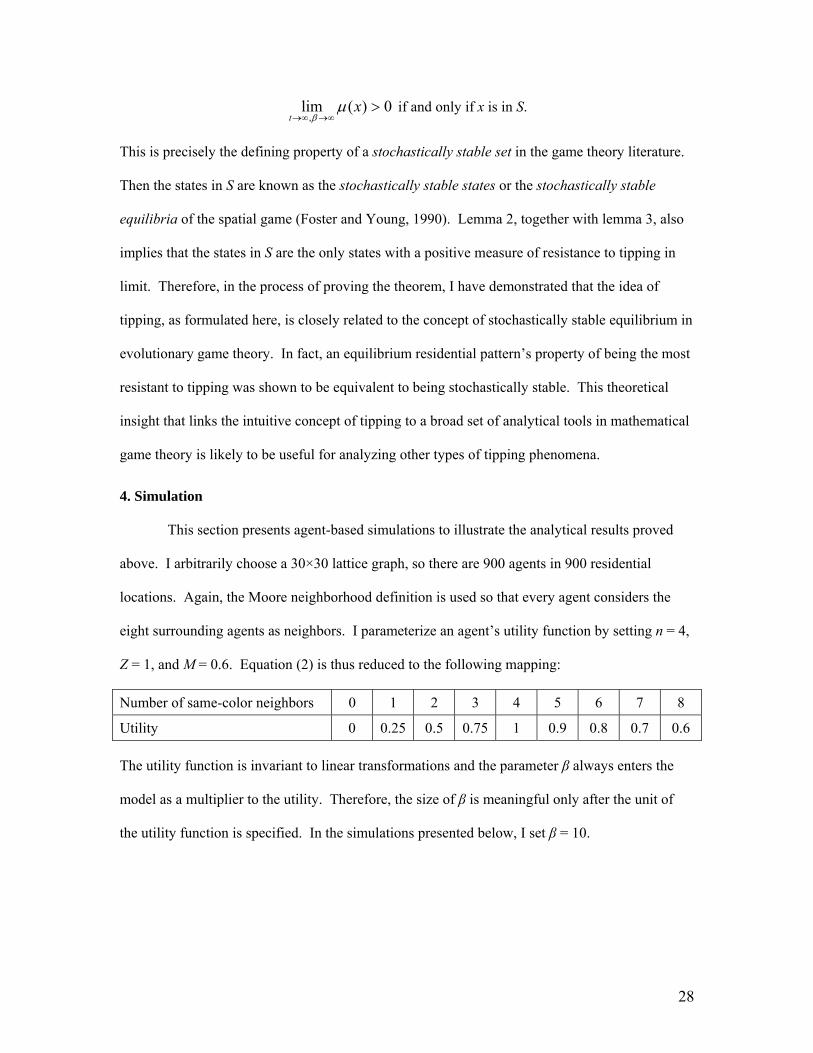
4. Simulation

This section presents agent-based simulations to illustrate the analytical results proved

above. I arbitrarily choose a 30×30 lattice graph, so there are 900 agents in 900 residential

locations. Again, the Moore neighborhood definition is used so that every agent considers the

eight surrounding agents as neighbors. I parameterize an agent’s utility function by setting n = 4,

Z = 1, and M = 0.6. Equation (2) is thus reduced to the following mapping:

Number of same-color neighbors 0 1 2 3 4 5 6 7 8

Utility 0 0.25 0.5 0.75 1 0.9 0.8 0.7 0.6

The utility function is invariant to linear transformations and the parameter β always enters the

model as a multiplier to the utility. Therefore, the size of β is meaningful only after the unit of

the utility function is specified. In the simulations presented below, I set β = 10.

28

The first simulation starts from the residential pattern labeled as “stripes,” in which two

rows of blacks always follow two rows of whites (panel (a) in Figure 5).33 A typical agent in this

initial state has five same-color neighbors. Although this is not the most preferred situation from

an agent’s point of view, the two groups are fairly integrated throughout the area. As discussed

above, this is an equilibrium state and only utility-decreasing switches can move the system out

of the initial state.

Indeed, in a typical run of the simulation, the initial state stays unchanged for some time

after the simulation starts. However, this usually does not last long before some mistaken

switches occur. And before such mistaken switches are reversed, some other mistaken ones

follow. As panel (b) in Figure 5 shows, a series of utility-decreasing switches have been made

mistakenly, which has moved the system fairly far away from its original equilibrium. In the

initial state, the total number of unlike neighboring pairs is 1260 (the value of “Rho” shown at the

bottom of panel (a)). In panel (b), this number has increased to 1359, as a result of all the

mistaken switches. By now, the system is out of equilibrium and many pairs of agents can

increase their utilities by trading residential locations if they are chosen to consider a switch.

Such moves continue to happen over time and the total number of unlike neighboring pairs

continues to decline. As panel (c) of Figure 5 shows, the whole area has evolved into a rather

segregated residential pattern. In the long run, as shown in panel (d), complete segregation

emerges. Every now and then, mistaken moves still occur, which increases the value of ρ, but

they only happen occasionally and never push ρ back too high. Thus complete segregation

persists over time.34

33 As indicated in the previous section, the results in the model do not depend on the proportion of the population that is black. In the simulations presented here, the numbers of blacks and whites are chosen to be either roughly the same (as in this first simulation) or exactly the same (as in the next one). This choice is somewhat arbitrary, but it does have one advantage. It clearly shows that the results of the model have nothing to do with the fact that blacks are a minority group in most U.S. cities. 34 Note that the persistence of segregation at the city level is not inconsistent with radical transitions at the neighborhood level. Consider the highly segregated city illustrated in panel (d) of Figure 5. Although the overall segregational pattern is not changing, the color line can still move over time. As a result, some of

29

Figure 6 traces the evolution of ρ, which helps illustrate how tipping occurred to the

original equilibrium. For some time after the simulation starts, the value of ρ does not change.

As mentioned above, this is because the starting state is an equilibrium and any switch in that

situation will decrease utilities and thus will happen with a very small probability given a fairly

large β. Eventually, such mistaken moves are taken and the value of ρ increases. The

accumulation of the mistaken moves soon pushes the system beyond a tipping point, which is

shown as the ρ function reaches its maximum in Figure 6. After that point, the ρ function

declines rather sharply because many agents find that they can increase their utilities by trading

residential locations. However, each such switch actually takes the system one step further

toward complete segregation. Occasionally, utility-decreasing switches still happen as indicated

by the small increases in ρ, but the probability of such events is too small to stop the evolution of

the system into complete segregation.

In Figure 6, the small values of the ρ function at the right end correspond to highly

segregated residential patterns. In theory, the probability of reversing the process and moving

back to the initial state is still positive. However, pushing the ρ function so high requires a large

number of utility-decreasing switches. Given that such switches happen with slim chances, the

probability that a large number of them happen one after another is virtually zero. Thus, it is

almost certain that the tipping of the original equilibrium is irreversible.

The second simulation, shown in Figure 7, starts with a checkerboard pattern. This initial

state is not only the most integrated residential pattern but also the socially optimal one because

exactly half of every agent’s neighbors are the same color. However, in the long run, it is also

tipped into complete segregation. Most interestingly, as shown by the evolution of the ρ function

the white neighborhoods close to the color line may change into black neighborhoods and vice versa. Some of these changes at the neighborhood level may even be described as “neighborhood tipping,” which does not lead to drastic changes in the residential pattern at the city level. Therefore, tipping at the city level (as the focus of this paper) is not exactly the same as tipping of a single neighborhood (as studied in Schelling’s original papers and others’ follow-up work); one does not necessarily imply the other.

30

in Figure 8, this Pareto optimal state is in fact less resistant to tipping than the “stripes”

equilibrium just discussed above. The ρ function in the initial state is at its maximum, and thus

no switches will increase ρ. This means that no switches will decrease the moving agents’

utilities. The tipping of this equilibrium state occurs immediately as the ρ function starts to

decrease right away; reversing the process is not likely to happen because it takes a large number

of utility-decreasing switches to do so.

What happened to this socially optimal state is instructive. In the initial state, everybody

lives in a half-half mixed neighborhood, thus it is not a bad idea to switch because after a switch

both agents still end up in a half-half neighborhood. Thus agents are not restrained from trading

residential locations. However, they ignore the externalities they create by their moves. Consider

a black agent in the initial state who decides to trade residential location with a white agent. Both

still have half black neighbors and half white neighbors after the switch. In the neighborhood the

black agent just left, all her neighbors will lose a black neighbor and have one more white

neighbor; each of them now has a lower utility than before. Neither the black agent who is

moving out nor the white agent who is moving in takes these losses of utilities into account.

After their switch, some blacks have 62.5 percent (or 5/8) white neighbors, and some whites have

62.5 percent black neighbors. By assumption, if a black with 62.5 percent white neighbors trades

residential location with a white with 62.5 percent black neighbors, both attain higher utilities.

As a result, they are likely to do it. Unfortunately, as they make the switch, they push both

neighborhoods even further away from the half-half balance. This leaves some of their previous

neighbors even more discontent with their neighborhoods and thus more agents will move. The

integrated residential pattern is soon broken and all the utility-increasing moves will only push

the system even further toward segregation.

Now the question is why a complete segregation cannot be tipped into a socially optimal

residential pattern given that nobody likes segregation. This simulation illustrates the answer.

31

Once complete segregation emerges, how much agents like integrated neighborhoods becomes

irrelevant in their moving decisions because very few locations (along the color line) qualify as

such neighborhoods. For example, a black agent living in an all-black neighborhood has

essentially two choices when considering a move. One is to trade with another black who lives in

another all-black neighborhood. In this case, the switch does not affect the overall residential

pattern. The other possibility is to trade with a white agent who lives in an all-white

neighborhood. In this case, both agents move from one extreme to the other. As assumed, if

integrated neighborhoods are unavailable, agents prefer to live with same-color neighbors. Thus

the move is a bad deal for both agents and will be unlikely to occur.

Therefore, although everybody prefers a socially optimal integrated residential pattern, it

is not stable. Too many utility-preserving moves can disturb this equilibrium and tip it into

segregation. On the other hand, although nobody likes complete segregation, the residential

pattern is very stable. Only moving across the color line by a considerable number of agents

could disturb the segregation equilibrium, but nobody has incentive to do so because it causes a

loss of utility.

This gives one plausible explanation for why segregation is persistent in U.S.

metropolitan areas despite the stated preference for integration. Segregation is stable not because

people like it, but because any individual who wants to change the situation unilaterally will have

to go across the color line, which may not be the desirable thing to do from the individual’s

perspective. A similar point was first emphasized by Zhang (2004a).

Some insights from economics can help us better understand the outcome of the model.

The failure of the system to escape complete segregation is similar to the phenomenon of

“coordination failure” studied by economists in many other contexts. It is the agents’ inability to

move simultaneously that make them stuck in a situation nobody likes.35 The fact that the

35 Many segregational outcomes in Schelling-type models may be understood as coordination failures. See, e.g., Hoff and Sen (2005) and Zhang (2004a).

32

socially optimal integrated neighborhoods are prone to tipping has to do with the notion of

externality.36 It is the exclusion of the external costs (imposed on neighbors) in the agents’

decision to move that makes the Pareto optimal residential pattern fall apart. Similarly, it is the

exclusion of the external benefits from the agents’ decision to move that keeps complete

segregation stable. A perfect analogy to this result in welfare economics is that a competitive

market equilibrium fails to produce a Pareto optimal allocation of resources if there exist

consumption externalities.37

5. Conclusion

In a series of writings, Schelling (1969, 1971, 1972, and 1978) presents two dynamic

models of residential segregation. His checkerboard model uses simulations to show that

segregational residential patterns are consistent with various individual preferences, including

those with only a moderate inclination to live with same-color neighbors. His neighborhood

tipping model demonstrates that seemingly unimportant random shocks could shake a

neighborhood out of one equilibrium situation and move it to another equilibrium that is radically

different. Using these models, Schelling teaches us that it is difficult to infer “micromotives”

from observed “macrobehavior” (Schelling, 1978).

In this paper, I presented a Schelling-type checkerboard model that can be rigorously

analyzed. I have shown that segregation emerges and persists in an all-integrationist world where

everybody prefers to live in a mixed-race neighborhood, a result consistent with Zhang (2004a)

and Pancs and Vriend (2007) but stronger than Schelling’s original finding. Schelling’s idea of

tipping, which has always been used in a single-neighborhood setting, is now introduced into the

36 Some earlier research on segregation and neighborhood transition also emphasized neighborhood externalities. See, e.g., Bond and Coulson (1989), Borjas (1995), Miyao (1978), and Schnare (1976). 37 The situation implies that there is a potential improvement of social welfare through government intervention. One way to achieve it may be to arrange a socially desirable residential pattern and limit individuals’ ability to move afterwards. The constraint on residential choice can take the form of either direct government regulation on certain types of moves or market-based policies such as taxes on or subsidies to certain types of moves. Singapore has a public housing policy with ethnic integration as a primary goal, which was indeed inspired by Schelling’s work (Dodge, 2006, Chapter 17, pp. 141-143).

33

multi-neighborhood checkerboard model. I have demonstrated that tipping occurs in this

checkerboard model in the sense that the accumulation of low-probability random events can

perturb an equilibrium residential pattern and trigger the move into a completely different

equilibrium residential pattern. The concept of tipping is crucial for understanding the dynamics

of segregation in this checkerboard model. Indeed, segregation emerges and persists precisely

because tipping tends to occur to integrated residential patterns but not to completely segregated

ones. Schelling’s insights, illustrated in his two separate models of segregation, are therefore

unified into a single model.

This unified model helps us better understand the persistence of segregation in U.S.

metropolitan areas during the past few decades. Following Schelling’s work, it points out the

possibility that segregation persists not because people really like it, but because it is a stable state.

As the model shows, tipping away from segregation is difficult because the first step involves

some blacks moving into predominantly white neighborhoods or some whites moving into

predominantly black neighborhoods or both. If people really dislike being isolated in a

neighborhood of the opposite color, as survey data seem to suggest, they will not take the first

step even though they really like “half black, half white” neighborhoods. Thus, they get stuck

with segregation.

This paper is by no means suggesting that segregation will stay forever as a salient

feature of urban America. Survey data show that individual residential preferences in the United

States have become more favorable toward the general notion of integration (Bobo, 2001). If this

trend continues, two conditions of the model may no longer be satisfied in the future. First, the

aversion to a neighborhood of the opposite color may fade away (i.e., the asymmetry in the utility

function disappears). Second, racial preferences may stop being the primary factors that drive

residential location decisions (i.e., parameter β is not sufficiently large). In both cases,

segregational housing patterns are not stable anymore. Indeed, some recent studies have found

that stable integrated neighborhoods, although still rare, are becoming more common (see, e.g.,

34

Ellen, 2000 and Rawlings et al., 2004), which may be an indication that we are moving in the

direction toward integration.

As a key theoretical contribution of this paper, I have established a link between the often

loosely formulated idea of tipping and the stochastically stable equilibrium, a rigorous

equilibrium concept in evolutionary game theory. I have shown that a residential pattern’s

property of being the most resistant to tipping is equivalent to being a stochastically stable

equilibrium. Because of this theoretical insight, a rich collection of analytical tools in stochastic

evolutionary game theory becomes useful for analyzing tipping phenomena.38 Given that

tipping-type dynamics are commonly observed, I anticipate that the method developed in this

paper will find its applications in some other contexts.

This paper can be extended in different directions. First, much analytical work remains

to be completed. To keep the model tractable, I have made a set of rather strong assumptions.

For example, housing market and non-racial neighborhood characteristics are ignored; racial

preferences are symmetric between groups and identical within each group; and moving

opportunities come up independently of agents’ satisfaction or dissatisfaction with their current

neighborhoods. Future research may explore which of these assumptions are crucial for the

analytical results and which can be relaxed.

Second, the model in this paper can also be used to motivate empirical work. For

example, the model predicts that residents’ unwillingness to move across the color line is the

crucial factor to make segregation persistent. One could collect survey data in different cities and

test the theory by correlating individuals’ answers to this question and the degree of segregation

at the city level, similar to what Cutler et al. (1997) and Card et al. (2008a) did in their papers.

The model also predicts that given the asymmetric residential preference, segregation would

persist if parameter β is large, i.e., if racial preference is the key factor in driving residential

location choices. This, in principle, can also be tested empirically.

38 For a comprehensive introduction of stochastic evolutionary game theory, see Young (1998).

35

Appendix: Proofs

Proof of Lemma 1: The equation holds trivially when the two agents are of the same color. We only need to deal with the case where the two agents are of different colors.

Consider the following two types of moves: (1) Both agents have less than half same-color neighbors to begin with and thus both will have more than half same-color neighbors after the switch. (2) One agent has more than half same-color neighbors and the other has less than half, and the opposite is true after the switch. These two types of switches and their reverse ones constitute all possible moves in the model and thus it suffices to show that the condition holds in these two cases.

Consider case (1). Suppose agent A has n-a same-color neighbors and agent B has n-b

same-color neighbors, 0≤a≤n and 0≤b≤n. After the switch, A will have n+b same-color neighbors and B will have n+a same-color neighbors. The effect on ρ is summarized as follows:

Before switch After switch Resultant change in ρ

A’s # of same-color neighbors n-a n+b -(a+b)

B’s # of same-color neighbors n-b n+a -(a+b) This switch also affects A’s and B’s neighbors, but because ρ is defined as unordered

pairs of unlike neighbors, it will be double counting if one also considers those neighbors. So the total effect on ρ is -2(a+b). That is, the total number of unlike neighboring pairs will decrease by 2(a+b) as a result of this switch.

The two agents’ utilities before and after the switch can be summarized as follows:

Before switch After switch Net gain

A’s utility Z(n-a)/n (2Z-M)+(M-Z)(n+b)/n [Mb+Z(a-b)]/n

B’s utility Z(n-b)/n (2Z-M)+(M-Z)(n+a)/n [Ma+Z(b-a)]/n The total net gain from the switch is thus (Ma+Mb)/n = -2(a+b)*[-M/(2n)] = Δρ*[-

M/(2n)], meaning that the total change in the agents’ utilities is proportional to the change in ρ. Consider case (2). Suppose agent C has n-c same-color neighbors and agent D has n+d

same-color neighbors, 0≤c≤n and 0≤d≤n. After the switch, C will have n-d same-color neighbors and D will have n+c same-color neighbors. The effect on ρ is summarized as follows:

Before switch After switch Resultant change in ρ

C’s # of same-color neighbors n-c n-d d-c

D’s # of same-color neighbors n+d n+c d-c The total effect on ρ is 2(d-c). That is, the total number of pairs of unlike neighbors will

change by 2(d-c) as a result of this switch.

36

These two agents’ utilities before and after the switch can be summarized as follows:

Before switch After switch Net gain

C’s utility Z(n-c)/n Z(n-d)/n Z(c-d)/n

D’s utility (2Z-M)+(M-Z)(n+d)/n (2Z-M)+(M-Z)(n+c)/n (M-Z)(c-d)/n The total net gain from the switch is thus M(c-d)/n = 2(d-c)*[-M/(2n)] = Δρ*[-M/(2n)],

still proportional to the change in ρ, and the multiplier of Δρ is the same -M/(2n). Therefore we have established that ρ(·|switch) - ρ(·|not switch) = -λ{[u(si|switch) +

u(sj|switch)] - [u(si|not switch) + u(sj|not switch)]}, where λ=2n/M>0. Q.E.D.

Proof of Lemma 2: For any two states x and y, let Pyx be the transition probability from state y to state x and myx the expected number of time periods for the system, starting from state y, to arrive at state x. Starting from state y, let’s assume 1 period has passed and examine the expected number of additional time periods it takes for the system to arrive at state x. With probability Pyx the system is already in x and it takes 0 additional time periods. With probability Pyk the system is in state k≠x, and it takes mkx periods to arrive at x. Therefore, myx can be written as

∑∑≠≠

+=+⋅+=xk

kxykxk

kxykyxyx mPmPPm 101 .

Multiply both sides of the equation by μ(y) and sum over all states to obtain

.)(1)(1

)()()(

∑∑ ∑

∑∑∑∑

≠≠

≠

+=+=

+=

xkkx

xk yykkx

xk ykxyk

yyyx

kmPym

mPyymy

μμ

μμμ

This implies that xxxk

kxy

yx mxmkmy )()()(1 μμμ =−= ∑∑≠

. It immediately follows that

μ(x)=1/mxx=r(x). Q.E.D.

Proof of Lemma 3: This result is a special case of theorem 6.1 in Young (1998). Let X be the set of all states and define a function π: X→[0,1] as follows

∑

=

∈

−

−

Xz

z

x

e

ex)(

)(

)(ρ

λβ

ρλβ

π .

Let Pxy be the transition probability from state x to y. It is straightforward to check that π(x) satisfy the detailed balance condition π(x)Pxy = π(y)Pyx. If x = y or Pxy = Pyx = 0, function π trivially satisfies the detailed balance condition. If x ≠ y and Pxy ≠ 0 or Pxy ≠ 0, then it must be true that x and y differ only at two locations. In the case the agents at these two locations are chosen, a switch between them will change the state from one to the other. There are a total of N2 agents on the lattice graph, therefore these two agents will be chosen with probability 1/[N2(N2-2n-1)]. (It is assumed that the two agents chosen are not neighbors, and thus once one is chosen, its 2n neighbors won’t be considered.) Let γ=1/[N2(N2-2n-1)], it follows that

37

[ ]

[ ] [ ] [ ]

[ ] [ ]

[ ]

.)(

)(

)(

)(

)()(

)(

)(

) |()|() |() |(

)(

)(

) |() |()|()|() |() |(

)(

)(

)|()|(

)(

)(

)(

)(

yxVU

V

Xz

z

y

VU

xyV

Xz

z

x

VU

switchnotswitchswitchnotsuswitchnotsu

Xz

z

x

VU

switchnotsuswitchnotsuswitchsuswitchsuswitchnotsuswitchnotsu

Xz

z

x

VU

switchsuswitchsu

Xz

z

x

VU

U

Xz

z

x

xy

Pyee

e

e

e

eee

e

e

eee

e

e

eee

e

e

eee

e

e

eee

e

ePx

ji

jijiji

ji

πγ

γ

γ

γ

γ

γπ

ββ

β

ρλβ

ρλβ

ββ

ρρλββ

ρλβ

ρλβ

ββ

ρρλββ

ρλβ

ρλβ

ββ

βββ

ρλβ

ρλβ

ββ

β

ρλβ

ρλβ

ββ

β

ρλβ

ρλβ

=⎭⎬⎫

⎩⎨⎧

+⋅=

⎪⎭

⎪⎬

⎫

⎪⎩

⎪⎨

⎧

+⋅=

⎪⎭

⎪⎬

⎫

⎪⎩

⎪⎨

⎧

+⋅=

⎭⎬⎫

⎩⎨⎧

+⋅=

⎭⎬⎫

⎩⎨⎧

+⋅=

⎭⎬⎫

⎩⎨⎧

+⋅=

∑

∑

∑

∑

∑

∑

∈

−

−

−−

∈

−

−

⋅−⋅−+

∈

−

−

+−+++

∈

−

−

+

∈

−

−

∈

−

−

Therefore, )(1)()()()( yyPyPyPxXx

yxXx

yxXx

xy πππππ =⋅=== ∑∑∑∈∈∈

, which means that

function π is a stationary distribution of the perturbed process. Because the Markov process is finite and irreducible, it has a unique stationary distribution. Given that μ is a stationary distribution of the process, it must be true that μ(x) = π(x) for any state x. It follows that

cxexeexx Xz

z+−∑−−

=== ∈

−)(ln)(

)(

)()(ρ

λβρ

λβ ρ

λβ

πμ , where ∑∈

−−=

Xz

zec

)(ln

ρλβ

is a constant. This

implies that states with minimum ρ have the highest probability of being visited. In the long run, with a β close to infinity, such states are observed almost all of the time.

Q.E.D.

38

References

Anas, Alex (1980), “A Model of Residential Change and Neighborhood Tipping,” Journal of Urban Economics 7, 358-370.

Aydinonat, N. Emrah (2005), “An Interview with Thomas C. Schelling: Interpretation of Game Theory and the Checkerboard Model,” Economics Bulletin 2, 1−7.

Bayer, Patrick, Robert McMillan, and Kim S. Rueben (2004), “What Drives Racial Segregation? New Evidence Using Census Microdata,” Journal of Urban Economics 56, 514-535.

Becker, Gary S. and Kevin M. Murphy (2000), Social Economics: Market Behavior in a Social Environment, Harvard University Press, Cambridge, MA.

Blume, Lawrence E. (1993), “The Statistical Mechanics of Strategic Integration,” Games and Economic Behavior 5, 387-424.

Blume, Lawrence E. (1997), “Population Games,” in W.B. Arthur, S.N. Durlauf, and D.A. Lane (Eds.), The Economy as an Evolving Complex System II, Addison-Wesley, Reading, MA, 425-460.

Bobo, Lawrence (2001), “Racial Attitudes and Relations at the Close of the Twentieth Century,” in N. Smelser, W. J. Wilson, and F. Mitchell (eds.), America Becoming: Racial Trends and Their Consequences, Washington, DC: National Academy Press, 264-301.

Bobo, Lawrence and Camille L. Zubrinsky (1996), “Attitudes on Residential Integration: Perceived Status Differences, Mere In-Group Preference, or Racial Prejudice?” Social Forces 74, 883-909.

Bog, Martin (2006), “Is Segregation Robust?” mimeo, Stockholm School of Economics.

Bond, Eric W. and N. Edward Coulson (1989), “Externalities, Filtering and Neighborhood Change,” Journal of Urban Economics 26, 231-249.

Borjas, George J. (1995), “Ethnicity, Neighborhoods, and Human-Capital Externalities,” American Economic Review 85, 365-390.

Bowles, Samuel (2003), Microeconomics: Behavior, Institutions, and Evolution, Princeton University Press, Princeton, NJ.

Brock, William A. and Steven N. Durlauf (2001), “Interaction-Based Models,” in J.J. Heckman and E.E. Leamer (Eds.), Handbook of Econometrics 5, North-Holland, Amsterdam, 3297-3380.

Bruch, Elizabeth E. and Robert D. Mare (2006), “Neighborhood Choice and Neighborhood Change,” American Journal of Sociology 112, 667–709.

Card, David and Jesse Rothstein (2007), “Racial Segregation and the Black–White Test Score Gap,” Journal of Public Economics 91, 2158-2184.

Card, David, Alexandre Mas, and Jesse Rothstein (2008a), “Tipping and the Dynamics of Segregation,” Quarterly Journal of Economics 123, 177–218.

Card, David, Alexandre Mas, and Jesse Rothstein (2008b), “Are Mixed Neighborhoods Always Unstable? Two-Sided and One-Sided Tipping,” NBER Working Paper No. 14470.

Charles, Camille Zubrinsky (2001), “Processes of Residential Segregation,” in Alice O’Connor, Chris Tilly, and Lawrence Bobo (eds.), Urban Inequality: Evidence From Four Cities, New York: Russell Sage Foundation.

Charles, Camille Zubrinsky (2003), “The Dynamics of Racial Residential Segregation,” Annual Review of Sociology 29, 167-207.

39

Clampet-Lundquist, Susan and Douglas S. Massey (2008), “Neighborhood Effects on Economic Self-Sufficiency: A Reconsideration of the Moving to Opportunity Experiment,” American Journal of Sociology 114, 107-143.

Clark, William A. V. (1991), “Residential Preferences and Neighborhood Racial Segregation: A Test of the Schelling Segregation Model,” Demography 28, 1-19.

Clark, William A. V. and Julian Ware (1997), “Trends in Residential Integration by Socioeconomic Status in Southern California,” Urban Affairs Review 32, 825–843.

Cloutier, Norman R. (1982), “Urban Residential Segregation and Black Income,” Review of Economics and Statistics 64, 282-288.

Courant, Paul N. (1978), “Racial Prejudice in a Search Model of the Urban Housing Market,” Journal of Urban Economics 5, 329-345.

Crane, Jonathan (1991), “The Epidemic Theory of Ghettos and Neighborhood Effects on Dropping out and Teenage Childbearing,” American Journal of Sociology 96, 1226-1259.

Cutler, David M. and Edward L. Glaeser (1997), “Are Ghettos Good or Bad?” Quarterly Journal of Economics 112, 827–872.

Cutler, David M., Edward L. Glaeser, and Jacob L. Vigdor (1999), “The Rise and Decline of the American Ghetto,” Journal of Political Economy 107, 455-506.

Darden, Joe T. and Sameh M. Kamel (2000), “Black Residential Segregation in the City and Suburbs of Detroit: Does Socioeconomic Status Matter?” Journal of Urban affairs 22, 1-13.

Davis, James A. and Tom W. Smith (1993), General Social Surveys, 1972-1993: Cumulative Codebook, National Opinion Research Center, University of Chicago.

Dawkins, Casey J. (2004), “Recent Evidence on the Continuing Causes of Black-White Residential Segregation,” Journal of Urban Affairs 26, 379–400.

Dodge, Robert (2006), The Strategist: The Life and Times of Thomas Schelling, Hollis Publishing Company, Hollis, NH.

Dokumaci, Emin and William H. Sandholm (2006), “Schelling Redux: An Evolutionary Dynamic Model of Residential Segregation,” mimeo, Department of Economics, University of Wisconsin.

Easterly, William (2005), “Empirics of Strategic Interdependence: The Case of the Racial Tipping Point,” mimeo, Department of Economics, New York University.

Ellen, Ingrid Gould (2000), Sharing America's Neighborhoods: The Prospects for Stable Racial Integration, Harvard University Press.

Emerson, Michael O., George Yancy, and Karen J. Chai (2001), “Does Race Matter in Residential Segregation? Exploring the Preferences of White Americans,” American Sociological Review 66, 922–35.

Epstein, Joshua M. and Robert Axtell (1996), Growing Artificial Societies: Social Science from the Bottom Up, Brookings Institution Press, Washington, D.C.

Fagiolo, Giorgio, Marco Valente, and Nicolaas J. Vriend (2007), “Segregation in Networks,” Journal of Economic Behavior and Organization 64, 316-336.

Farley, John E. (1995), “Race Still Matters: The Minimal Role of Income and Housing Cost as Causes of Housing Segregation in St. Louis, 1990,” Urban Affairs Review 31, 244-254.

Farley, Reynolds, Elaine L. Fielding, and Maria Krysan (1997), “The Residential Preferences of Blacks and Whites: A Four-Metropolis Analysis,” Housing Policy Debate 8, 763-800.

40

Farley, Reynolds and William H. Frey (1994), “Changes in the Segregation of Whites from Blacks during the 1980s: Small Steps toward a More Integrated Society,” American Sociological Review 59, 23-45.

Farely, Reynolds, Howard Schuman, Suzanne Bianchi, Diane Colasanto, and Shirley Hatchett (1978), “‘Chocolate City, Vanilla Suburbs’: Will the Trend toward Racially Separate Communities Continue?” Social Science Research 7, 319-344.

Farley, Reynolds, Charlotte Steeh, Maria Krysan, Tara Jackson, and Keith Reeves, (1994), “Stereotypes and Segregation: Neighborhoods in the Detroit Area,” American Journal of Sociology 100, 750-780.

Fossett, Mark (2006), “Ethnic Preferences, Social Distance Dynamics, and Residential Segregation: Theoretical Explorations Using Simulation Analysis,” Journal of Mathematical Sociology 30, 185-273.

Foster, Dean, and H. Peyton Young (1990), “Stochastic Evolutionary Game Dynamics,” Theoretical Population Biology 38, 319-332.

Galster, George C. (1987), “Residential Segregation and Interracial Economic Disparities: A Simultaneous-Equations Approach,” Journal of Urban Economics 21, 22-44.

Gladwell, Malclm (2000), The Tipping Point: How Little Things Can Make a Big Difference, Little, Brown and Company, Boston, MA.

Glaeser, Edward L. and Jacob Vigdor (2001), “Racial Segregation in the 2000 Census: Promising News,” Center on Urban and Metropolitan Policy, The Brookings Institution, Wahsington, D.C. (available at http://www.brook.edu/es/urban/census/glaeser.pdf accessed on March 7, 2007).

Goering, John M. (1978), “Neighborhood Tipping and Racial Transition: A Review of Social Science Evidence,” Journal of the American Institute of Planners 44, 68 – 78.

Goering, John M. and Ron Wienk (ed.) (1996), Mortgage Lending, Racial Discrimination and Federal Policy, Urban Institute Press.

Granovetter, Mark (1978) “Threshold Models of Collective Behavior,” American Journal of Sociology 83, 1420-1443.

Granovetter, Mark and Roland Soong (1983), “Threshold Models of Diffusion and Collective Behavior,” Journal of Mathematical Sociology 9, 165-179.

Granovetter, Mark and Roland Soong (1988), “Threshold Models of Diversity: Chinese Restaurants, Residential Segregation, and the Spiral of Silence,” Sociological Methodology 18, 69-104.

Heal, Geoffrey and Howard Kunreuther (2006), “Tipping and Supermodularity,” Mimeo, School of Business, Columbia University.

Hoff, Karla and Arijit Sen (2005), “Homeownership, Community Interactions, and Segregation,” American Economic Review 95, 1167-1189.

Iceland, John and Rima Wilkes (2006), “Does Socioeconomic Status Matter? Race, Class, and Residential Segregation,” Social Problems 53, 248–273.

Kain, John (1968), “Housing Segregation, Negro Employment, and Metropolitan Decentralization,” Quarterly Journal of Economics 82, 175-197.

Kern, Clifford R. (1981), “Racial Prejudice and Residential Segregation: The Yinger Model Revisited,” Journal of Urban Economics 10, 164-172.

41

Kling, Jeffrey R., Jeffrey B. Liebman, and Lawrence F. Katz (2007), “Experimental Analysis of Neighborhood Effects,” Econometrica 75, 83-119.

Krysan, Maria and Reynolds Farley (2002), “The Residential Preferences of Blacks: Do They Explain Persistent Segregation?” Social Forces 80, 937-980.

Logan, John R., Brian J. Stults, and Reynolds Farley (2004), “Segregation of Minorities in the Metropolis: Two Decades of Change,” Demography 41, 1-22.

Ludwig, Jens, Jeffrey B. Liebman, Jeffrey R. Kling, Greg J. Duncan, Lawrence F. Katz, Ronald C. Kessler, and Lisa Sanbonmatsu (2008), “What Can We Learn about Neighborhood Effects from the Moving to Opportunity Experiment?” American Journal of Sociology 114, 144-188.

Massey, Douglas and Nancy Denton (1993), American Apartheid: Segregation and the Making of the Underclass, Cambridge, MA: Harvard University Press.

McFadden, Daniel (1973), “Conditional Logit Analysis of Qualitative Choice Behavior,” in Zarembka, P. (ed.), Frontier in Econometrics, Academic Press, New York, 105–142.

Miyao, Takahiro (1978), “Dynamic Instability of a Mixed City in the Presence of Neighborhood Externalities,” American Economic Review 68, 454-463.

Mobius, Markus M. (2000), “The Formation of Ghettos as a Local Interaction Phenomenon”, mimeo, Department of Economics, Harvard University.

Monderer Dov and Lloyd S. Shapley (1996), “Potential Games,” Games And Economic Behavior 14, 124–143.

Orfield, Gary and Susan E. Eaton (1996), Dismantling Desegregation: The Quiet Reversal of Brown v. Board of Education, New York: The New Press.

O'Sullivan, Arthur (2008), “Schelling’s Model Revisited: Residential Sorting with Competitive Bidding for Land,” unpublished manuscript, Lewis & Clark College.

Pancs, Romans and Nicolaas J. Vriend (2007), “Schelling's Spatial Proximity Model of Segregation Revisited,” Journal of Public Economics 91, 1–24.

Rawlings, Lynette, Laura Harris, Margery Austin Turner, and Sandra Padilla (2004), “Race and Residence: Prospects for Stable Neighborhood Integration,” No. 3 in the Neighborhood Change in Urban America Series, Urban Institute, Washington, D.C.

Ross, Stephen L. and Margery A. Turner (2005), “Housing Discrimination in Metropolitan America: Explaining Changes between 1989 and 2000,” Social Problems 52, 152–180.

Royal Swedish Academy of Sciences (2005a), “Robert Aumann’s and Thomas Schelling’s Contributions to Game Theory: Analyses of Conflict and Cooperation,” available at http://nobelprize.org/nobel_prizes/economics/laureates/2005/ecoadv05.pdf (accessed December 20, 2006).

Royal Swedish Academy of Sciences (2005b), “The Prize in Economic Sciences 2005,” supplementary information to press release, available at http://nobelprize.org/nobel_prizes/economics/laureates/2005/info.pdf (accessed December 20, 2006).

Ruoff, Gabriele and Gerald Schneider (2006), “Segregation in the Classroom: An Empirical Test of the Schelling Model,” Rationality and Society 18, 95-117.

Schelling, Thomas C. (1960), The Strategy of Conflict, Harvard University Press, Cambridge, MA.

42

Schelling, Thomas C. (1969), “Models of Segregation,” American Economic Review (Papers and Proceedings) 59(2), 488-493.

Schelling, Thomas C. (1971), “Dynamic Models of Segregation,” Journal of Mathematical Sociology 1, 143-86.

Schelling, Thomas C. (1972), “A Process of Residential Segregation: Neighborhood Tipping,” in Pascal, Anthony (ed.), Racial Discrimination in Economic Life, D. C. Heath, Lexington, MA, 157-84.

Schelling, Thomas C. (1978), Micromotives and Macrobehavior, Norton, New York, NY.

Schelling, Thomas C. (2006), Strategies of Commitment and Other Essays, Harvard University Press, Cambridge, MA.

Schnare, Ann B. (1976), “Racial and Ethnic Price Differentials in an Urban Housing Market,” Urban Studies 13, 107-120.

Schnare, Ann B. and C . Duncan MacRae (1978), “The Dynamics of Neighbourhood Change,” Urban Studies 15, 327-331.

Schuman, Howard, Charlotte Steeh, Lawrence Bobo, and Maria Krysan (1997), Racial Attitudes in America: Trends and Interpretations, revised edition, Cambridge, MA: Harvard University Press.

Sethi, Rajiv and Rohini Somanathan (2004), “Inequality and Segregation,” Journal of Political Economy 112, 1296-1321.

Shihadeh, Edward S. and Nicole Flynn (1996), “Segregation and Crime: The Effect of Black Social Isolation on the Rates of Black Urban Violence,” Social Forces 74, 1325-1352.

Taeuber, Karl E. (1968), “The Effect of Income Redistribution on Racial Residential Segregation,” Urban Affairs Quarterly 4, 5-14.

Taylor, Howard M. and Samuel Karlin (1998), An Introduction to Stochastic Modeling, 3rd edition, Academic Press, San Diego, CA.

Vigdor, Jacob L. (2003), “Residential Segregation and Preference Misalignment,” Journal of Urban Economics 54, 587–609.

Wasmer, Etienne and Yves Zenou (2002), “Does City Structure Affect Job Search and Welfare?” Journal of Urban Economics 51, 515–541.

Williams, David R. and Chiquita Collins (2001), “Racial Residential Segregation: A Fundamental Cause of Racial Disparities in Health,” Public Health Reports 116, 404–416.

Wilson, William J. (1987), The Truly Disadvantaged: The Inner City, the Underclass, and Public Policy, Chicago: University of Chicago Press.

Yinger, John (1976), “Racial Prejudice and Racial Residential Segregation in an Urban Model,” Journal of Urban Economics 3, 383-396.

Yinger, John (1986), “Measuring Racial Discrimination with Fair Housing Audits: Caught in the Act,” American Economic Review 76, 881-893.

Yinger, John (1995), Closed Doors, Opportunities Lost: The Continuing Costs of Housing Discrimination, Russell Sage Foundation, New York, NY.

Young, H. Peyton (1998), Individual Strategy and Social Structure: An Evolutionary Theory of Institutions, Princeton University Press, Princeton, NJ.

43

44

Young, H. Peyton (2001), “The Dynamics of Conformity,” in Durlauf, S. N. and Young, H. P. (eds.), Social Dynamics, Brookings Institution Press/MIT Press, Washington, D.C./Cambridge, MA, 133–153.

Zhang, Junfu (2003), “Revisiting Residential Segregation by Income: A Monte Carlo Test,” International Journal of Business and Economics 2, 27-37.

Zhang, Junfu (2004a), “Residential Segregation in an All-Integrationist World,” Journal of Economic Behavior and Organization 54, 533-550.

Zhang, Junfu (2004b), “A Dynamic Model of Residential Segregation,” Journal of Mathematical Sociology 28, 147-170.

Figure 1: An agent’s utility as a function of neighborhood racial composition

Figure 2: Moore neighborhood

Figure 3: Equilibrium residential patterns

(a) (b)

(c) (d)

Figure 4: Tipping between two equilibrium states in a restricted process

Value of ρ a b c

Communicating states

Figure 5: Tipping of an equilibrium residential pattern (“stripes”)

(a) (b)

(c) (d)

Figure 6: Evolution of the potential function, starting with an equilibrium residential pattern (“stripes”)

0

200

400

600

800

1000

1200

1400

1600

0 4000 8000 12000 16000 20000 24000 28000

Time

Num

ber o

f unl

ike

neig

hbor

ing

pairs

(Rho

)

Figure 7: Tipping of the socially optimal residential pattern

(a) (b)

(c) (d)

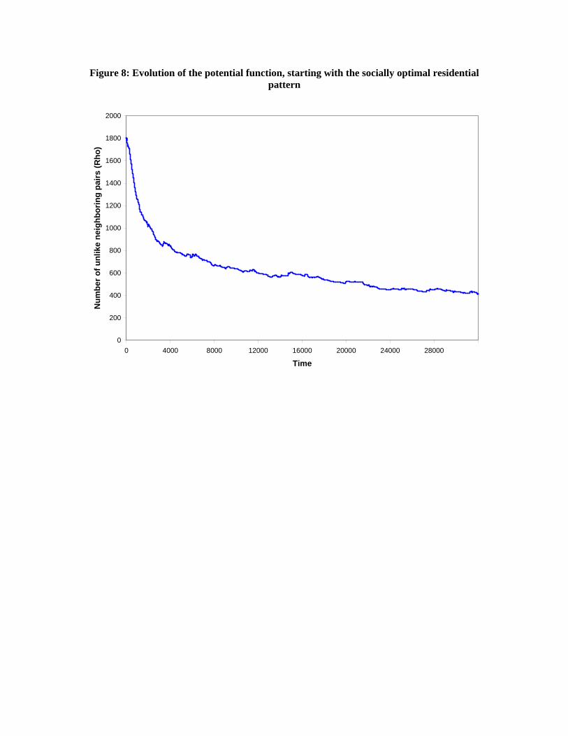
Figure 8: Evolution of the potential function, starting with the socially optimal residential pattern

0

200

400

600

800

1000

1200

1400

1600

1800

2000

0 4000 8000 12000 16000 20000 24000 28000

Time

Num

ber o

f unl

ike

neig

hbor

ing

pairs

(Rho

)