Chapter 9

TIME VARYING FIELDS, TEMWAVES IN UNBOUNDED MEDIAAND TRANSMISSION LINES

9.1 Introduction

The magnetic �eld is created by a current which is driven by the electric �eld

E! J = �E! r�B = �0J

In short, an electric �eld can produce a magnetic �eld. Can the process be reversed, that is, can a

magnetic �eld produce an electric �eld? The answer to this question was given by Faraday in 1831

who, after painstaking attempts, found that a time varying magnetic �ux induces an emf,

emf = � d

dt (9.1)

where (Weber) is the magnetic �ux. This law is known as the Faraday�s law, and it is perhaps

the most important discovery in electrodynamics both in practical applications (generation of emf)

and in fundamental formulation of electromagnetic �elds.

If a time varying magnetic �eld induces an electric �eld, can a time varying electric �eld induce

a magnetic �eld? The answer to this question was given by Maxwell who generalized the Ampere�s

law in static cases

r�B = �0J

to

r�B =�0�J+�0

@E

@t

�(9.2)

so that the charge conservation law@�

@t+r � J = 0

1

can be self-consistently satis�ed by Ampere�s law. The discovery of the displacement current �0@E

@tis of fundamental importance because it was with this new term that Maxwell was able to predict

that electromagnetic disturbances can propagate even in vacuum in the form of electromagnetic

waves.

In this Chapter, we allow time varying nature for all �elds to formulate complete Maxwell�s

equations in general cases. Then, based on the Maxwell�s equations, we will derive a wave equation

for electromagnetic �elds, and consider special modes of wave propagation called TEM (transverse

electric and magnetic) modes in free space and also in transmission lines. The concept of wave

impedance will turn out to be useful in analyzing re�ection and transmission at a boundary of

di¤erent media.

9.2 Faraday�s Law

In 1831, Faraday (accidentally) discovered that in the con�guration shown in Figure 9.1, switch-

ing the current on and o¤ in the primary loop induces a current in the secondary loop. If the

switch is kept closed, no such induction is observed no matter how large the dc current is. What

is responsible for induction is the change in the current, that is, the change in the magnetic �ux

coupled to the secondary loop. This monumental discovery is formulated in the following form,

emf =IE � dl = � d

dt = � d

dt

ZB � dS V (9.3)

The minus sign in front of the time variation of the magnetic �ux is due to Lenz, and indicates

that the emf is induced so as to oppose the change in the magnetic �ux. For example, in Figure

9.2(a), the North pole of a magnet is approaching a conducting loop. The magnetic �ux coupled to

the loop is increasing with time because the magnetic �eld is stronger near the pole, and the emf

induced along the loop is clockwise if seen from top. In Fig. 9.2(b), the magnetic �eld is decreasing

(still upward), and the emf is counterclockwise. Even when the magnetic �eld is not time varying

explicitly, an emf is still induced if the magnetic �ux enclosed by a closed loop is varying with time.

For example, if a conducting rod placed on sliding rails moves across a constant magnetic �eld, as

shown in Figure 9.3, the magnetic �ux enclosed by the loop is decreasing with time, and an emf is

induced. This so-called motional emf is in fact the basic principle of most generators, and Faraday

performed several experiments on this e¤ect. Realizing that river water is electrically conducting

(because of pollutants), he tried to measure an emf to be induced across the River Thames �owing,

of course, across the earth magnetic �eld, but failed because of insu¢ cient sensitivity of equipment

available at that time.

The appearance of the motional emf can be seen from Eq. (9.3) as follows. The change in the

magnetic �ux through an area S consists of two parts, one due to the explicit time variation in the

2

S

V

A

Figure 9-1: Faraday discovered that current was induced in the secondary loop when the swith Swas closed or opened. In steady state, no induction was observed.

magnetic �eld, and the other due to the change in the area,

d

dt

ZB � dS =

Z@B

@t� dS+

ZB � @

@tdS (9.4)

where

dS = dl1 � dl2 (9.5)

is the area element in terms of the length elements in the plane perpendicular to dS. Since

@

@t(dl1 � dl2) = v1 � dl2 + dl1 � v2 = v1 � dl2 � v2 � dl1

= v � dl (9.6)

where v is the velocity at which the length element dl is moving, and

B � (v � dl) = (B� v)�dl (9.7)

we may rewrite IE � dl = �d

dt

as IE � dl = �

Z@B

@t� dS�

I(B� v) � dl; (9.8)

where v is now understood as the velocity of the material volume element. Removing the integralsigns in Eq. (9.8), we obtain

r�E = �@B@t

+r� (v �B) (9.9)

Even in a stationary magnetic �eld, @B=@t = 0, an observer (or an object) moving with a velocity

3

B decreasing

N

S

N

S

I I

B increasing

v

v

a b

Figure 9-2: (a) North pole of a bar magnet approaching a conducting loop. The induced current isclockwise if seen from top. (b) The magnet is moving away from the loop. The current is reversed

v in a magnetic �eld experiences an e¤ective electric �eld given by

Em = v �B (9.10)

This �eld is called the motional electric �eld.

v

B into page

I

Figure 9-3: Induction of emf when a conductor loop is moving across a magnetic �eld.

An example of device wholly dependent on the motional emf is the MHD (magnetohydrody-

namic) generator, which converts kinetic energy of weakly ionized gas (plasma) directly into electric

energy. When an ionized gas is injected perpendicular to a magnetic �eld, an electric �eld given in

4

Eq. (9.10) is induced. Ions and electrons are thus separated, and migrate toward electrodes sand-

wiching the plasma. If the electrodes are connected through a load resistor R, direct conversion of

plasma kinetic energy into electric energy occurs without any rotational mechanical components.

The output voltage is directly porportional to the product vB, and the need for a large mag-

netic �eld is apparent. For economical MHD power generation, superconducting magnets will be

required.

The Hall e¤ect is caused by the same mechanism. When a current carrying conductor is placed

perpendicular to a magnetic �eld, the current carriers (either electrons or holes) experience v �Belectric �eld, and charge separation occurs. The direction of the induced voltage (or the current)

depends on the kind of carriers. Furthermore, the induced voltage is proportional to IB, and the

Hall e¤ect is extensively used in devices to measure the intensity of magnetic �eld.

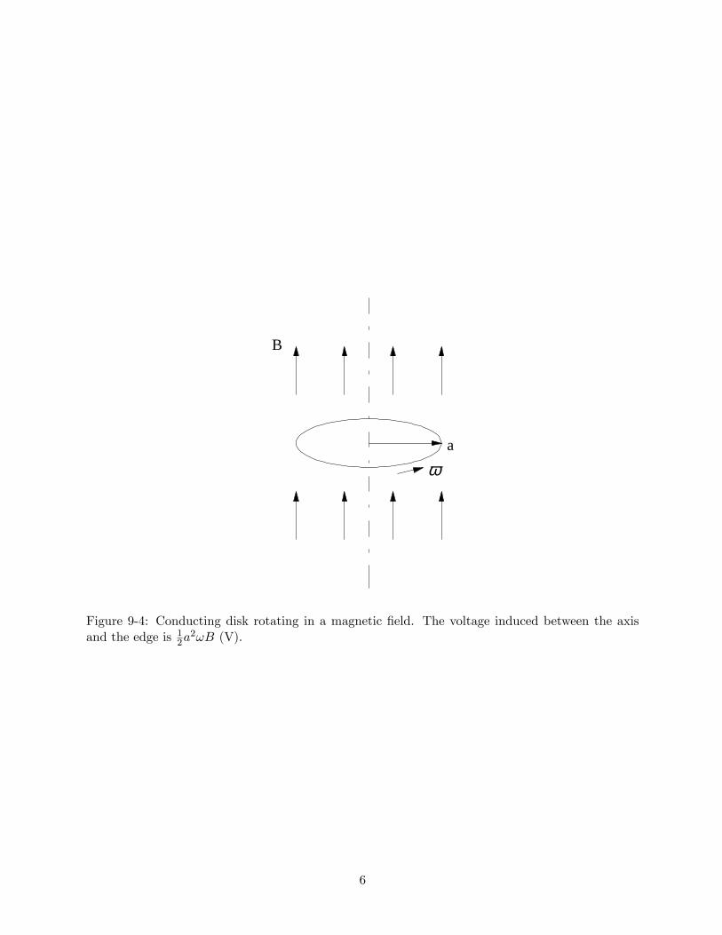
Homopolar GeneratorA conducting disk of radius a is rotating about its center in a plane perpendicular to a stationary

magnetic �eld B. The area swept by a radius in time dt is

dS =1

2a2!dt

where ! is the angular rotation frequency in rad/sec. Then,

d = BdS =1

2Ba2!dt

and the magnitude of the induced emf is found to be

emf =1

2!Ba2 (V) (9.11)

Figuring out the direction of emf is left for the reader.

Surprisingly, the formula obtained in the above example also applies to a cylindrical permanent

magnet rotating about its axis. This was known to Faraday. In this case, the magnetic �eld

is stationary, and there is no sign of time variation of magnetic �ux enclosed by any closed loop

either. What is essential for motional emf is the fact that a conductor is moving across a magnetic

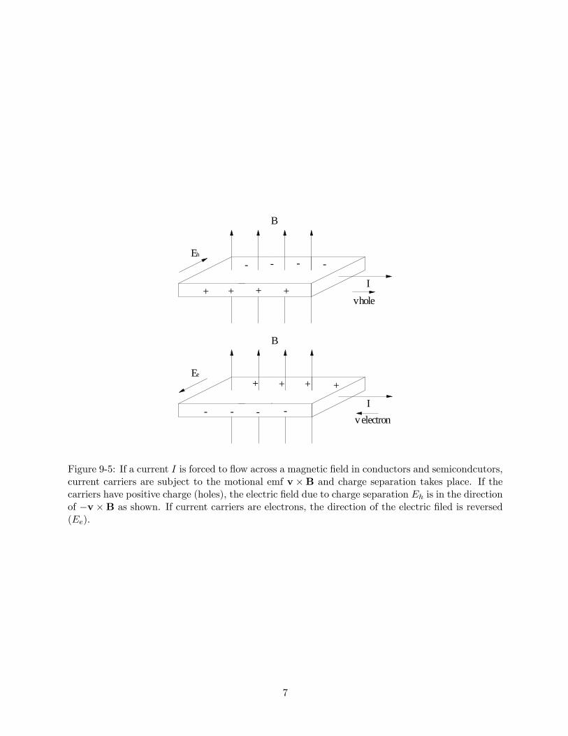
�eld.Hall E¤ect, MHD GeneratorWhen a current carrying conductor is placed in a magnetic �eld, the current carriers experinece

a motional emf,

Em = v �B

where v is the velocity of curent carriers. In semiconductors, current carrier is either electron

(negative charge) or hole (positive charge). The carriers are then shifted in the direction v � B(holes) or �v�B (electrons) and from this Hall voltage, the sign of charge of current carriers can

be determined. This principle is used in Hall meters to measure the intensity of magnetic �eld.

In MHD (magnetohydrodynamic) generator, a plasma (ionized gas) is force to move across a

strong magnetic �eld. Resultant Hall electric �eld can be used for power generation.

5

a

B

ω

Figure 9-4: Conducting disk rotating in a magnetic �eld. The voltage induced between the axisand the edge is 12a

2!B (V).

6

I

B

+ + + +

­ ­ ­ ­Eh

I

B

+ + + +

­ ­ ­ ­

Ee

vhole

v electron

Figure 9-5: If a current I is forced to �ow across a magnetic �eld in conductors and semicondcutors,current carriers are subject to the motional emf v �B and charge separation takes place. If thecarriers have positive charge (holes), the electric �eld due to charge separation Eh is in the directionof �v �B as shown. If current carriers are electrons, the direction of the electric �led is reversed(Ee):

7

q

Jr

Figure 9-6: A charged body is losing its charge at the rate I = �dq=dt; I = 4�r2Jr where Jr is theradial current density. There is no magnetic �eld even though there is a current.

9.3 Displacement Current

That the Ampere�s law

r�B = �0 J (Ampere�s law) (9.12)

is not consistent with the fundamental charge conservation law

@�

@t+r � J = 0 (9.13)

can be readily seen if we note the vector identity

r � (r�B) = 0 (9.14)

Therefore, for time varying �elds, the Ampere�s law must be modi�ed somehow to be consistent

with the charge conversation law. This modi�cation (or generalization) was done by Maxwell. Let

us see what new term should be added to the RHS of Eq. (9.12) in a simple model.

Consider a charged body which is losing charge radially outward at a rate

dq

dt= �I (A) (9.15)

where

I = 4�r2Jr (9.16)

is the radially outward current, and Jr is the current density at radius r. Since the electric �eld at

the same position is given by

Er =1

4��0

q

r2(9.17)

8

we �nd@Er@t

= � 1

4��0

I

r2= �Jr

�0(9.18)

or

Jr + �0@Er@t

= 0 (9.19)

Because of the spherical symmetry of the system, there can be no magnetic �elds even though we

do have a conduction current Jr. In other words, the magnetic �eld which would be created by the

conduction current is to be cancelled by another current,

�0@Er@t

�or �0

@E

@t

�(displacement current) (9.20)

so that

(r�B)r = �0

�Jr + �0

dErdt

�= 0:

The newly introduced current

�0@E

@t(A/m2) (9.21)

is called the displacement current, and the generalized Ampere�s law is given by

r�B =�0�J+ �0

@E

@t

�(9.22)

The charge conservation law is now identically satis�ed,

@�

@t+r � J = @�

@t� @

@tr � (�0E) =

@�

@t� @�

@t= 0 (9.23)

to our comfort.

The generalized Ampere�s law,

r�B = �0

�J+ �0

@E

@t

�indicates that a magnetic �eld can be induced by a time varying electric �eld as well as by a

conduction current, J. Even when there are no conduction currents (J = 0), a magnetic �eld maybe induced entirely by a time varying electric �eld. Together with the Faraday�s law, Maxwell

was able to predict that even in vacuum, electromagnetic disturbance propagates as a wave which

transfers electromagnetic energy from one location to another.

Consider a parallel plate capacitor being charged at a rate

I =dq

dt

9

B

B

B ?

I

­ ­ ­­­ ­

­ ­

Figure 9-7: Is there a magnetic �eld in a capacitor being charged? There is no conduction currentin a capacitor.

In the capacitor, there is no conduction current but there is a displacement current,

�a2"0dE

dt= �a2"0

d

dt

�V

d

�= �a2"0

1

Cd

dq

dt=dq

dt; C =

"0�a2

d

which is eqaul to the charging current. There is a magnetic �eld in the capacitor, that can be found

from

2�rB� = �0r2

a2I

B� =�0I

2�a2r; r < a

9.4 Poynting�s Theorem and Lumped Constant Circuit Approxi-mation

The complete set of the Maxwell�s equations is thus given by

r �E = �

�0(9.24)

r�E = �@B@t

(9.25)

r �B =0 (9.26)

r�B = �0

�J+ �0

@E

@t

�(9.27)

10

where the charge density � and current density J are related through the charge conservation law

@�

@t+r � J = 0

Any electromagnetic phenomena should be consistent with these four laws. So far, not a single

experimental evidence has been found to contradict with these laws, even in subatomic scales

and highly relativistic cases. The Maxwell�s equations are all in di¤erential form and describe

local electric and magnetic �elds. In contrast, dc and ac circuit theories deal with macroscopic

quantities, such as voltage and current. The macroscopic circuit theories should also be consistent

with the Maxwell�s equations. Let us consider a typical series RLC circuit driven by a low frequency

generator, V (t) = V0ej!t: The Kirchho¤�s voltage theorem yields

V (t) = Ri+ Ldi

dt+1

C

Zi dt (9.28)

Here it should be noted that the current i(t) has been assumed to be independent of the location in

the circuit, that is, the phase di¤erence in the currents has been entirely ignored. This assumption

is subject to the condition that the system size of the circuit is small enough so that the speed of

electromagnetic propagation can be regarded in�nitely large, or what amounts to the same thing,

the system size is much smaller than the wavelength associated with the generator frequency !,

circuit size� c

!(9.29)

Therefore, steady state ac circuit theory is applicable only in low frequency limit. As the frequency

increases, the wavelength becomes shorter, and the phase di¤erence along the circuit becomes

important. In this case, spatial variation of the voltage and current must be taken into account

in the analysis. This leads us to wave equations for voltage and current as will be shown in the

following section.

Quiz 1: Why is that there are four Maxwell�s equations?

Multiplying Eq. (9.28) by i(t), we �nd the following power conservation law,

V i = Ri2 +d

dt

�1

2Li2�+d

dt

�1

2

q2

C

�(9.30)

where

i(t) =dq

dt

is noted for the capacitor. The Kirchho¤�s voltage law is therefore a consequence of power (or

energy) conservation law. (Similarly, the Kirchho¤�s current theorem is a consequence of the

charge conservation law.)

Let us see how this macroscopic energy conservation law is consistently satis�ed by the Maxwell�s

11

equations. For this purpose, we �rst calculate the area integral of the vector E�H,I(E�H)�dS (W) (9.31)

The vector E�H has the dimensions of W/m2, the power density, and is called the Poynting

vector. Using the Gauss�theorem, we convert this into a volume integral,I(E�H) � dS =

Zr � (E�H) dV =

Z(H�r �E�E�r �H) dV (9.32)

Substituting r�E;r�H from Eqs. (9.25) and (9.27), respectively, we obtainI(E�H) � dS = �

Z �@

@t

�1

2�0H

2

�+@

@t

�1

2�0E

2

�+E � J

�dV (9.33)

The power �ux in the LHS is outward from the volume V . Therefore, the inward �ux is just the

negative of the surface integral, and we obtain

�I(E�H) � dS = power �owing into volume V =

Zv

�@

@t

�1

2�0H

2 +1

2�0E

2

�+E � J

�dV

(9.34)

The physical meaning of each quantity in the volume integral is obvious. The �rst term

@

@t

�1

2�0H

2 +1

2�0E

2

�(W/m2) (9.35)

indicates the rate of magnetic and electric energy storing, and the second term, E � J; is the Jouledissipation,

E � J = �E2 = �J2 (W/m3) (9.36)

For a circuit involving a single inductor, the magnetic energy may be de�ned byZ1

2�0H

2dV =1

2Li2 (9.37)

Similarly, Z1

2�0E

2dV =1

2

q2

C(9.38)

de�nes the capacitive energy, and the Joule dissipation term de�nes the resistance,ZE � J dV = Ri2 (9.39)

Again, it should be noted that these macroscopic, lumped constants (L;C;R) can be well de�ned

only in a low frequency limit. If the Poynting �ux is integrated over an arbitrary closed surface

containing the generator, it should yield the total power delivered to the LCR circuit.

12

R

E x H

E x H

E x H

V

Figure 9-8: Poynting vector in a simple dc circuit is directed from the generattor to the loadeverywhere.

In a simple dc circuit shown in Fig. ??, the Poynting vector is directed toward the load resistoreverywhere and its integral is equal to the power dissipated in the resisotr,Z

E�H � dS = V 2

R

9.5 Wave Equations for Electromagnetic Fields in Source-Free Re-gions

Let us consider electromagnetic �elds in free space which contains no sources, � = 0;J = 0. The

Maxwell�s equations in this case become

r �E = �

�0= 0 (� = 0) (9.40)

r�E = �@B@t

(9.41)

r �B = 0 (9.42)

r�B =�0�0@E

@t(J = 0) (9.43)

Of course, to create electromagnetic �elds, we must have sources somewhere, but we assume that

they are located far away from the region where we wish to analyze the �elds. Taking curl of Eq.

(9.41) and recalling the assumption r �E = 0, we �nd

r�r�E = r(r �E)�r2E = �r2E = � @

@tr�B (9.44)

Substituting r�B from Eq. (9.43), we obtain

r2E = 1

c2@2E

@t2(9.45)

13

where

c =1

p�0�0

= 3:0� 108m/ sec (9.46)

is the speed of light in vacuum. A similar equation can be obtained for the magnetic �eld by taking

curl of Eq. (9.43),

r2B = 1

c2@2B

@t2(9.47)

Both Eqs. (9.45) and (9.47) are wave equations, and their solutions in various coordinate systems

have been exhaustively studied.

Let us consider the simplest case, a plane electromagnetic wave. A plane wave is characterized by

a constant amplitude and unidirectional wave propagation. We assume that a wave is propagating

in the z direction at a speed c. Then, spatial variation occurs only in z direction, and thus,

r = ez@

@zin Eqs. (9.45) and (9.47). Eq. (9.45) thus reduces to

@2

@z2E(z; t) =

1

c2@2

@t2E(z; t) (9.48)

Without loss of generality, we may assume E(z; t) = Ex(z; t)ex, that is, only the x component of

electric �eld for a plane wave. Then, Eq. (9.48) further reduces to a scalar wave equation,

@2

@z2Ex(z; t) =

1

c2@2

@t2Ex(z; t) (9.49)

General solutions to this wave equation are

Ex(z; t) = F (z � ct) (9.50)

where F is an arbitrary, well-behaving function. This may be readily proved if we introduce a

function

X = z � ct:

Since@

@z=@X

@z

d

dX=

d

dX;@2

@z2=

d2

dX2;@

@t=@X

@t

d

dX= �c d

dX;@2

@t2= c2

d2

dX2;

we see that Eq. (9.49) is identically satis�ed if the electric �eld depends on z and t in the form given

in Eq. (9.50). The function F is arbitrary. It may be of sinusoidal form as in most applications,

or pulse, step function, etc. However, as we know from Fourier analysis, any waveforms can be

constructed by a collection of sinusoidal waves. Therefore, studying the wave equation for a single

sinusoidal wave is su¢ cient.

If a source is oscillating with a frequency ! = 2�f , wave perturbation created by the source is

sinusoidal having a wavelength

� =c

f:

14

Then, as a solution for a sinusoidal plane wave, we may assume

Ex(z; t) = E0 exphj!�t� z

c

�i= E0 exp [j (!t� kz)] (9.51)

where

k =!

c(rad/m) =

2�

�(9.52)

is called the phase constant in engineering and wavenumber in physics. If the wave is propagating

in +z direction, the minus sign in Eq. (9.51) is to be chosen,

Ex(z; t) = E0ej(!t�kz) (9.53)

The solution with the plus sign in Eq. (9.51) indicates a wave propagating in �z direction.From Eq. (9.43), we see that the magnetic �eld is in the y direction,

B(z; t) = B0eyej(!t�kz) (9.54)

and the amplitudes E0 and B0 are related through

B0 =k

!E0 =

E0c

(9.55)

Recalling H = B=�0 in vacuum, we may alternatively use the vector H,

H(z; t) =

r�0�0E0eye

j(!t�kz)

=1

ZE0eye

j(!t�kz) (A/m) (9.56)

where

Z =

r�0�0= 377 (9.57)

is the impedance of free space. The Poynting vector

S = E�H (W/m2) (9.58)

is directed along the z direction, that is, the direction of wave propagation and thus energy propaga-

tion. It is related to the local electromagnetic energy density as follows. The electric and magnetic

energy densities are1

2�0E

2;1

2�0H

2:

However, E and H are related through the impedance Z as

E = ZH

15

Therefore,1

2�0E

2 =1

2�0�0�0H2 =

1

2�0H

2;

that is, in a plane electromagnetic wave, the electric energy density is identically equal to the

magnetic energy density everywhere and any time, and the total energy density is twice of either

energy,

Total energy density = �0E2�= �0H

2�

(J/m3) (9.59)

(It is customary to use the electric �eld E.) Since the speed of propagation is c, the rate of energy

transfer per unit time per unit area is

c�0E2 =

r�0�0E2 =

�=

r�0�0H2

�=

1

ZE2�= ZH2

�(W/m2) (9.60)

which is equal to the magnitude of the Poynting vector

jE�Hj = 1

ZE2 = ZH2:

It is important to recognize that any wave, be it mechanical or electromagnetic, that can be

described by a wave di¤erential equation is associated with two agents, each being able to store

di¤erent forms of energies. Sound waves in gases, solids and liquids are associated with potential

energy due to elasticity and kinetic energy due to motion of medium. In electromagnetic waves,

a medium should be able to store both electric and magnetic energies. Vacuum is an excellent

medium for electromagnetic waves because vacuum is indeed able to store both forms of energies.

(See, for example, �Introduction to Wave Phenomena�by Hirose and Lonngren.)

[x; 0; sin (2�x)]

Example: Electric Field in a Laser Beam

Let us calculate the intensities of electric and magnetic �elds of a laser beam having an rms power

density of 5� 1013 W/cm2. FromE2

Z= 5� 1017W=m2;

we �nd

Erms = 1:37� 1010 V=m:

The magnetic �eld is

Brms =Ermsc

= 45:8 T, or Hrms =ErmsZ

= 3:63� 107A=m:

The peak �eld intensities arep2 times of the rms values.

16

­0.5

1.0

­1.0

0.50.0

­0.50.0

0.5

0

1.0

­1.0 1

2

3

4

5

Figure 9-9: Plane electromagnetic wave. Electric �eld in red and magnetic �eld in blue. Wavelengthis 1 unit length.

Example: Poynting Flux in a Coaxial Cable

A resistor R () is connected to a dc power supply of V (volts) through a loss-less coaxial cable

having inner/outer radii of a=b. We wish to show that the area integral of the Poynting �uxZ b

aSz2��d�

in the coaxial cable is consistent with the rate of energy transfer, V 2=R (W).

The reader may wonder why this static (dc) problem has anything to do with electromagnetic

waves. The problem is not really static because we have a current �ow. Although the current is dc,

and thus the magnetic �eld is static, this problem is dynamic because energy �ow from the power

supply to the resistor indeed exists. The apparent static electric and magnetic �elds are established

after transient phenomena (right after the switch is closed) are over, and a simple dc circuit like in

this example is indeed a legitimate wave phenomenon.

If the cable resistance is ignored, the current is given by

I =V

R:

Then, the azimuthal magnetic �eld in the cable is

B�(�) =�oI

2��=�0V

2�R

1

�:

17

b2a

E

B

I

IRV

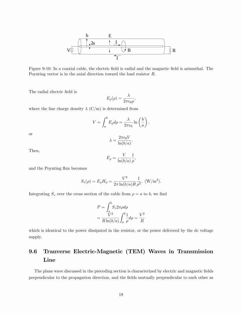
Figure 9-10: In a coaxial cable, the electric �eld is radial and the magnetic �eld is azimuthal. ThePoynting vector is in the axial direction toward the load resistor R:

The radial electric �eld is

E�(�) =�

2��0�;

where the line charge density � (C/m) is determined from

V =

Z b

aE�d� =

�

2��0ln

�b

a

�;

or

� =2��0V

ln(b=a):

Then,

E� =V

ln(b=a)

1

�;

and the Poynting �ux becomes

Sz(�) = E�H� =V 2

2� ln(b=a)R

1

�2; (W=m2):

Integrating Sz over the cross section of the cable from � = a to b, we �nd

P =

Z b

aSz2��d�

=V 2

R ln(b=a)

Z b

a

1

�d� =

V 2

R

which is identical to the power dissipated in the resistor, or the power delivered by the dc voltage

supply.

9.6 Tranverse Electric-Magnetic (TEM) Waves in TransmissionLine

The plane wave discussed in the preceding section is characterized by electric and magnetic �elds

perpendicular to the propagation direction, and the �elds mutually perpendicular to each other as

18

dz

i(z) i(z+dz)

V(z) V(z+dz)

dL

dC

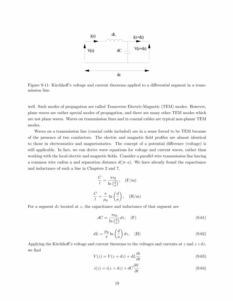
Figure 9-11: Kirchho¤�s voltage and current theorems applied to a di¤erential segment in a trans-mission line.

well. Such modes of propagation are called Transverse Electric-Magnetic (TEM) modes. However,

plane waves are rather special modes of propagation, and there are many other TEM modes which

are not plane waves. Waves on transmission lines and in coaxial cables are typical non-planar TEM

modes.

Waves on a transmission line (coaxial cable included) are in a sense forced to be TEM because

of the presence of two conductors. The electric and magnetic �eld pro�les are almost identical

to those in electrostatics and magnetostatics. The concept of a potential di¤erence (voltage) is

still applicable. In fact, we can derive wave equations for voltage and current waves, rather than

working with the local electric and magnetic �elds. Consider a parallel wire transmission line having

a common wire radius a and separation distance d(� a). We have already found the capacitance

and inductance of such a line in Chapters 2 and 7,

C

l=

��0

ln�da

� ; (F=m)

C

l=

�

�0ln

�d

a

�; (H=m)

For a segment dz located at z, the capacitance and inductance of that segment are

dC =��0

ln�da

�dz; (F) (9.61)

dL =�0�ln

�d

a

�dz; (H) (9.62)

Applying the Kirchho¤�s voltage and current theorems to the voltages and currents at z and z+dz,

we �nd

V (z) = V (z + dz) + dL@i

@t(9.63)

i(z) = i(z + dz) + dC@V

@t(9.64)

19

Taylor expanding V (z + dz); i(z + dz) as

V (z + dz) ' V (z) +@V

@zdz (9.65)

i(z + dz) ' i(z) +@i

@zdz (9.66)

we rewrite Eqs. (9.63) and (9.64) as

�@V@z

=L

l

@i

@t(9.67)

� @i@z=C

l

@V

@t(9.68)

from which we see that the voltage and current should satisfy the same wave equation,

@2V

@z2=1

c2@2V

@t2(9.69)

@2i

@z2=1

c2@2i

@t2(9.70)

whereL

l

C

l= �0�0 =

1

c2(9.71)

has been substituted.

Let us assume the following solutions for the wave equations,

V (z; t) = V0ej(!t�kz) (9.72)

i(z; t) = i0ej(!t�kz) (9.73)

From Eq. (9.67), we obtain

kV0 =!L

li0 (9.74)

However,!

k= c (9.75)

Then,

Z =V0i0=!

k

L

l=

sL=l

C=l=1

�

r�0�0ln

�d

a

�() (9.76)

This is the characteristic impedance of the parallel wire transmission line valid when d� a. Note

that it contains the impedance of free spacep�0=�0 = 377 . Other factors are due to the

geometrical con�guration of the transmission line which re�ects deviation from the plane wave in

free space although waves on a transmission line are still TEM.

A similar calculation for a coaxial cable (inner and outer radii a and b, �lled with an insulating

20

material having permittivity �) shows that the impedance of such cable is given by

Z =1

2�

r�0�ln

�b

a

�(9.77)

The propagation velocity is reduced by a factorp�=�0 from the velocity in free space,

c0 =1

p��0

(9.78)

In practice, the permittivity of any material exhibits rather strong dependence on the wave fre-

quency, � = �(!). Furthermore, in general, it is complex,

� = Re �+ j Im � ; Im � < 0 (9.79)

The condition of Im � < 0 is required from cuasality and indicates that the wave is damped because

of absorption by dielectrics.

In the analysis of a dc circuit involving a coaxial cable in Sec. 9.5, the impedance of the cable

did not appear at all, while for waves, Eq. (9.77) clearly indicates that the voltage and current

waves are related through the impedance,

V (z; t) = Z i(z; t) (9.80)

However, this relationship really originates from the basic equation, Eq. (9.67),

�@V@z

=L

l

@i

@t:

For dc current and voltages, all derivatives vanish, and the ratio V=i can be arbitrary. (Recall that

0/0 is inde�nite.) In fact, for the dc circuit analyzed in Sec. 9.5, the ratio is trivially determined

by the load resistance, which can be varied at will.

This apparent paradox can be resolved if we realize that a dc state is the �nal state of transient

phenomena in which multiple wave re�ections are involved. As we have seen in Sec. 9.6, the wave

equation such as@2V

@z2=1

c2@2V

@t2

can be satis�ed by an arbitrary function

V (z; t) = F (ct� z)

The current i (z; t) satis�es the same wave eqaution,

@2i

@z2=1

c2@2i

@t2

21

The function F is not necessarily a sinusoidal function, although in most practical applications, we

do encounter sinusoidal or harmonic waves. As we have already seen, a harmonic wave propagating

in the positive z direction can be written as

V (z; t) = V0ej(!t�kz) (9.81)

The phase function !t� kz is in the form ct� z since

!t� kz = !

�t� k

!z

�:

The constant k is called the phase constant in engineering and wavenumber in physics. For a

sinusoidal wave,

k =!

c=2�

�(rad/m) (9.82)

V (z; t) = F (ct+ z) (9.83)

indicates a wave propagating in the negative z direction. Most wave media are bilateral in the

sense that waves can be propagated in both directions. (Otherwise, telephone conversations would

be di¢ cult.)

The arbitrariness of the functional form F (ct � z) is, strictly speaking, valid only if the wave

speed c is frequency independent. In the discussion to follow, we assume that the propagation

speed is frequency independent.

Waves propagating in the negative z direction will occur when they are re�ected at a dis-

continuity in the characteristic impedance. Consider two transmission lines having characteristic

impedance Z1 and Z2, respectively. For simplicity, we assume both lines are loss-less so that the

impedances are pure real. An incident voltage wave, Vi, is sent toward the discontinuity on the line

1. The power associated with the incident wave is

V 2iZ1

(W) (9.84)

Let the wave on the line 2 be Vt (the subscript �t� for transmitted wave), and re�ected wave on

the line 1 be Vr which propagates in the negative z direction. The power associated with the

transmitted and re�ected waves are, respectively,

V 2tZ2;

V 2rZ1:

It is evident from energy (or power) conservation that the incident power is split into transmitted

and re�ected powers, and we haveV 2iZ1

=V 2rZ1

+V 2tZ2

(9.85)

The continuity in the tangential electric �elds at the impedance discontinuity is equivalent to the

22

continuity in the voltages because the voltage is to be evaluated from the integral of the electric

�eld. Therefore,

Vi + Vr = Vt (9.86)

Solving Eqs. (9.85) and (9.86) for Vr and Vt in terms of Vi, we obtain

Vr =Z2 � Z1Z2 + Z1

Vi (9.87)

Vt =2Z2

Z2 + Z1Vi (9.88)

Although we have derived these formulae for the case of pure real impedances, they in fact hold

true for complex impedances as well. The ratio between the re�ected and incident volatages,

VrVi� �V

is called the voltage re�ection coe¢ cient. � is a constant (complex in general) determined by the

impedances of connected lines.

Connecting an in�nitely long transmission line having an impedance Z2 at the end of a trans-

mission line having an impedance Z1 is equivalent to terminating the line with a resistance R = Z2

because if the line 2 is in�nitely long, no re�ection occurs on the line 2 and there is no way to

recover the power transmitted to the line 2. This irreversible power transmission can be considered

equivalent to irreversible Joule dissipation in a resistor, as long as the voltage and current in the

line 1 are concerned. When a line having an impedance Z1 is terminated by a resistor R, Eqs.

(9.99) and (9.100) are to be modi�ed as

Vr =R� Z1R+ Z1

Vi (9.89)

VR =2R

R+ Z1Vi (9.90)

where VR is the resistor voltage.

A similar re�ection formula can be worked out for the current using the power and current

conservation laws,

Z1i2i = Z1i

2r + Z2i

2t (9.91)

ii + ir = it (9.92)

The result is

ir =Z1 � Z2Z2 + Z1

ii (9.93)

it =2Z1

Z2 + Z1ii (9.94)

23

V

S

Z R

Figure 9-12: Transient evolution of the voltage wave when the swith S is closed.

Note that the incident, re�ected and transmitted waves satisfy

Viii= Z1 ;

Vrir= �Z1 ;

Vtit= Z2 (9.95)

The negative sign for the re�ected wave is due to wave (or energy) propagation in the negative

z direction. (The Poynting vector of the re�ected wave should be directed in -z direction.) Also

note that the current re�ection coe¢ ecient, ir=ii, is simply the negative of the voltage re�ection

coe¢ cient.

With these preparations, we are now ready to analyze the transient, multiple wave re�ections

on a transmission line terminated with a resistance R. In Fig. ??, the switch S is closed at t = 0.A step function voltage wave with an amplitude V0 starts propagating along the line at a speed c.

The current wave is also a step function with an amplitude

i =V0Z

(9.96)

This initial phase lasts until the waves reach the end where the resistor R is connected. The

duration of the initial stage is obviously � = l=c where l is the length of the transmission line. Note

that the initial waves do not know what is waiting at the end until they reach it. When the initial

waves reach the end, a re�ected voltage wave with an amplitude

Vr =R� ZR+ Z

V0 = �V0 (9.97)

starts propagating toward the power supply. Here, � is the voltage re�ection coe¢ cient at the load,

� =R� ZR+ Z

At the power supply, the voltage re�ection coe¢ cient is �1 if the power supply has a negligibleimpedance. Then, after 2� = 2l=c, a voltage wave having an amplitude �Vr starts propagatingtoward the load end. These multiple re�ections continue, and the �nal voltage on the transmission

line approaches

V0 + �V0 � �V0 � �2V0 + �2V0 + �3V0 � �3V0 � � � = V0 (9.98)

24

which is what is expected from dc theory. The current approaches

V0Z

�1� �� �� �2 � �2 � � � �

�=V0Z

�1� 2� 1

1 + �

�=V0Z

1� �1 + �

=V0R

(9.99)

also a result expected from dc theory. Therefore, what we calculate from dc theory is actually

the �nal stage of the wave transient phenomenon. In practical experiments, the transient is so

short that only with a fast measuring device (such as a high frequency oscilloscope) can we observe

such transient. It is important to realize that simple looking dc (or ac) circuits do involve wave

phenomena because energy transfer from a generator to a load can only be achieved in the form of

electromagnetic waves.

The condition to eliminate the re�ected wave at the load is that the load impedance be equal

to the characteristic impedance of the transmission line,

RL = Z (for impedance matching) (9.100)

In this case, the initial transient lasts only for the transit time, � = l=c, without any multiple

re�ections.

If light falls on a glass surface which has an index of refaction ng = 1:5; the power re�ection is

�2 =

�Zg � Z0Zg + Z0

�2=

11:5 � 111:5 + 1

!2= 0:04 = 4% per surface

Later we will learn how to eliminate re�ection by using a quarter wavelength transformer.

9.7 Steady-state Harmonic Waves in a Transmission Line

As explained in Section 9.4, the di¤erence between the ac circuit theory and wave theory is

mainly in the size of circuit system relative to the wavelength. In ac theory, it is assumed that

the wavelength � is su¢ ciently long compared with the system size so that phase shift due to

the system size is negligibly small. However, as the wave frequency ! increases, the wavelength

� becomes shorter, and the ac theory totally breaks down. The wave theory of transmission lines

was �rst successfully formulated by Heaviside at the end of the last century. (Heaviside is best

known for the operator method invented for solving di¤erential equations. This invention later

triggered extensive research on the theory of distributions which satisfactorily formulated such

singular functions as delta and step functions. The symbol r was also used for the �rst time

by Heaviside as a di¤erential operator in general coordinate systems.) Transient phenomena in a

transmission line are rather complicated to analyze. Here, we assume that a steady oscillating state

has been established after an initial transient phase. Let us consider the transmission line shown

in Fig. 9.18. A load impedance ZL terminates the line having a characteristic impedance Z0 and

25

and length l. It is a good practice to add a resistor Rg = Z0 at the generator end to ensure that at

least re�ection at this end is avoided. Otherwise, �ringing�caused by multiple re�ections occurs.

In contrast to ac theory, the impedance Zin seen by the generator becomes dependent on the

length of the transmission line. To �nd Zin, we assume that incident and re�ected voltage waves

are described by

Vi(z; t) = V0ej(!t�kz) (9.101)

Vr(z; t) = �(0)V0ej(!t�kz) (9.102)

As a reference, we choose z = 0 at the load end. �(0) is the voltage re�ection coe¢ cient at the

load end, z = 0. The generator end is thus at z = �l.The re�ection coe¢ cient at the load end, (0), is given by

�(0) =ZL � Z0ZL + Z0

(9.103)

At the generator end, z = �l, the incident and re�ected waves take the following values,

Vi(z = �l) = V0ej(!t�kl) (9.104)

Vr(z = �l) = �(0)V0ej(!t�kl) (9.105)

Therefore, the re�ection coe¢ cient at the generator end becomes

�(z = �l) = �(0)e�2jkl (9.106)

By de�nition, the re�ection coe¢ cient and the impedance Zin are related as

�(z = �l) = Zin � Z0Zin + Z0

= �(0)e�2jkl (9.107)

Solving Eq. (9.107) for Zin, we �nd

Zin(�l) =1 + � (0) e�2jkl

1� �(0)e�2jkl Z0 (9.108)

The impedance becomes strongly dependent on the length of the transmission line through the

factor e2jkl. If kl � 1, that is, if the wavelength is much longer than the transmission line, we

trivially recover the ac result,

Zin = ZL (kl� 1) (9.109)

The formula in Eq. (9.108) has important applications in impedance matching. If in Fig. 9.20,

the load impedance is equal to the line impedance Z0(RL = Z), we have complete impedance

matching. No wave re�ections occur, and the maximum available power from the generator having

26

Z ZZinL

l

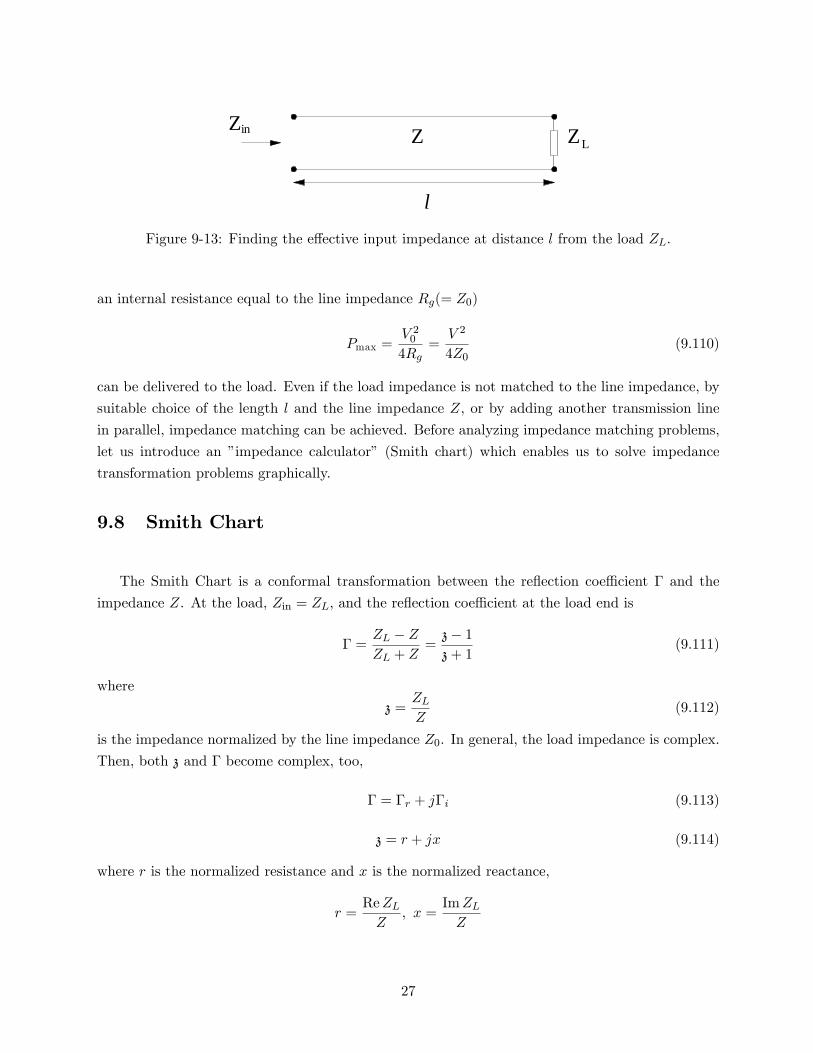
Figure 9-13: Finding the e¤ective input impedance at distance l from the load ZL:

an internal resistance equal to the line impedance Rg(= Z0)

Pmax =V 204Rg

=V 2

4Z0(9.110)

can be delivered to the load. Even if the load impedance is not matched to the line impedance, by

suitable choice of the length l and the line impedance Z, or by adding another transmission line

in parallel, impedance matching can be achieved. Before analyzing impedance matching problems,

let us introduce an �impedance calculator� (Smith chart) which enables us to solve impedance

transformation problems graphically.

9.8 Smith Chart

The Smith Chart is a conformal transformation between the re�ection coe¢ cient � and the

impedance Z. At the load, Zin = ZL, and the re�ection coe¢ cient at the load end is

� =ZL � ZZL + Z

=z� 1z+ 1

(9.111)

where

z =ZLZ

(9.112)

is the impedance normalized by the line impedance Z0. In general, the load impedance is complex.

Then, both z and � become complex, too,

� = �r + j�i (9.113)

z = r + jx (9.114)

where r is the normalized resistance and x is the normalized reactance,

r =ReZLZ

; x =ImZLZ

27

Solving Eq. (9.111) for z, we obtain

z =1 + �

1� � =1 + �r + j�i1� �r � j�i

(9.115)

or

r + jx =1� �2r � �2i + 2j�i(1� �r)2 + �2i

(9.116)

From the real part, we �nd ��r �

r

r + 1

�+ �2i =

1

(r + 1)2(9.117)

and from the imaginary part,

(�r � 1)2 +��i �

1

x

�2=1

x2(9.118)

Eq. (9.117) indicates a circle having a radius1

r + 1and its center located at

�r

r + 1; 0

�on the complex � plane. Similarly, Eq. (9.118) describes a circle with a radius 1=x, and its center

at �1;1

x

�The impedance Smith chart is shown in Fig. 9-14.

The impedance and the re�ection coe¢ cient have one-to-one correspondence with respect to

each other. If the impedance is known, the re�ection coe¢ cient can be read o¤ the Smith Chart, and

vice versa. The upper half of the Smith Chart corresponds to an inductive impedance, x > 0, while

the lower half corresponds to a capacitive impedance x < 0. A shorted end (z = 0) corresponds to

the point (�1; 0) on the �-plane, and an open end (z =1) is located at (+1, 0). The center of theSmith Chart � = 0 + j0 corresponds to a matched impedance,

z = 1 + j0 or ZL = Z0:

The re�ection coe¢ cient at the load end (z = 0), and that at a distance l from the load are

related through (see Eq. (9.108))

�(z = �l) = �(0)e�2jkl (9.119)

On the �-plane, �(�l) can be located by rotating the load point �(0) clockwise by an angle 2kl,or �toward the generator�. Note that one complete rotation corresponds to an increase in l by

one-half wavelength since 2kl = 2� is equivalent to l = �=2.

By choosing a suitable line length l, it is possible to make the input impedance Zin at z = �lpure real, or have its real part matched with the line impedance, as long as the load impedance has

28

x = 0

x = 0.5

x = 1x = 2

x = ­0.5x = ­1

x = ­2

r = 1/3r = 1

r = 3

short open

Figure 9-14: Impedance Smith chart.

a �nite resistive component. Let us work on a few examples.

Example: At what line length l=� does the input impedance (a) become pure real, (b) have a realpart equal to 50 ?

Let us solve by an analytic method �rst. The re�ection coe¢ cient at the load end is �(0) =100+j30�50100+j30+50 = 0:36 + j0:13 = 0:38ej0:343: Then, using Eq. (9.108), the input impedance at

length l becomes

Zin(�l) =1 + �(0)e�2jkl

1� �(0)e�2jklZ0

=1 + 0:38ej0:343

1� 0:38ej0:343Z0

=0:855 + j0:762 sin(0:343� 2kl)1:145� 0:762 cos(0:343� 2kl) Z0; Z0 = 50

(a) Pure real The impedance becomes pure real when

0:343� 2kl = �n�(n = 0; 1; 2; � � � )

or

29

� =4�l

�= 0:343 + n�

= 0:343; 0:343 + �; � � �

When 4�l=� = 0:343 (or l=� = 0:027), the impedance becomes

Zin = 2:23� 50 = 111:6

and when 4�l=� = 0:343 + �(l=� = 0:527),

Zin = 0:448� 50 = 22:4:

(b) Re Zin = 50

From

0:855 = 1:145� 0:762 cos(0:343� 2kl)

we �nd

cos(0:343� 2kl) = 0:381

or

2kl = 1:523; 2� � 0:837; � � �

These cumbersome calculations can be avoided if we use the Smith Chart. First, the normalized

load impedance zL = 2 + j0:6 is located at � (0) on the chart. As the line length l increases, this

point rotates clockwise and hits the horizontal axis at A, where the input impedance is pure real.

The impedance at A corresponds to the �rst solution Zin = 111:6 found in (a). Further increase

in l makes the vector � hit the r = 1 circle at B on which the real part of the impedance is 50 .

The point B is at angle 1.523 rad (' 87:3�) from the load point as found in (b). The second pure

real impedance occurs at C whose angular location is at � + 0:343, the second solution found in

(a). The real part of the impedance is 50 at D which is at an angle 2� � 0:837 found in (b) asthe second solution.

Quarter Wavelength MatchingWhen the line length is a quarter wavelength (l = �=4), the input impedance becomes

Zin =Z20ZL

(9.120)

This can be readily seen from Eq. (9.108) in which

e�2jkl = e�j� = �1:

30

x = 0short open

x = 0.6

r = 2Γ(0)

Α

B

C

Figure 9-15: The normalized load impedance z = 2 + i0:6 and its re�ection coe¤ecient � (0) islocated on the Smith chart. Impedance at distance �l (toward the generator) can be found byrotating � (0) by � = 2kl clockwise.

Thus

Zin =1� �(0)1 + �(0)

Z0 =1� ZL � Z0

ZL + Z0

1 +ZL � Z0ZL + Z0

=Z20ZL

(9.121)

For example, a line having impedance Z2 can be matched with a line with impedance Z1 by inserting

a line with an impedance

Z =pZ1Z2

in between provided its length is chosen to be a quarter wavelength. This principle is equivalent to

the well known quarter wavelength coating in optics to minimize wave re�ection. The impedance

of glass is typically 250 with a permittivity �g ' 2�0. In order to match the glass impedance withthat of air, Z = 377 , a dielectric �lm with an impedance

p250� 377 = 307 is coated on the

glass surface. The �lm permittivity is

�f =p�0�g ' 1:5�0:

Therefore, the speed of light in the �lm is smaller than that in free space by a factorp1:5 = 1.23

from which the coating thickness (�=4) can be determined for a desired wavelength in free space.

For example, green light has a wavelength in free space � ' 5500 Å. In the �lm, the wavelength

becomes 5500 Å=1:23 ' 4470 Å. Then, the coating thickness to minimize re�ection of green lightis 4470 Å=4 ' 1120 Å.

31

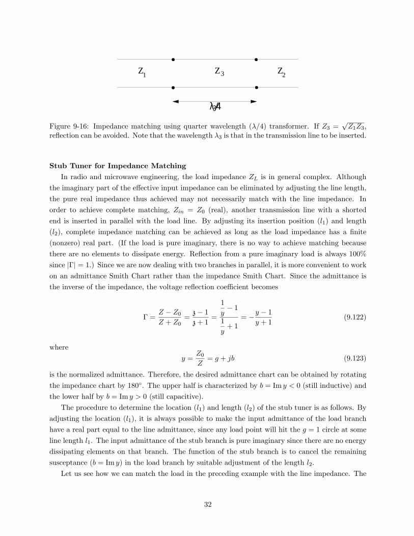
Z Z Z1 23

λ /43

Figure 9-16: Impedance matching using quarter wavelength (�=4) transformer. If Z3 =pZ1Z3;

re�ection can be avoided. Note that the wavelength �3 is that in the transmission line to be inserted.

Stub Tuner for Impedance MatchingIn radio and microwave engineering, the load impedance ZL is in general complex. Although

the imaginary part of the e¤ective input impedance can be eliminated by adjusting the line length,

the pure real impedance thus achieved may not necessarily match with the line impedance. In

order to achieve complete matching, Zin = Z0 (real), another transmission line with a shorted

end is inserted in parallel with the load line. By adjusting its insertion position (l1) and length

(l2), complete impedance matching can be achieved as long as the load impedance has a �nite

(nonzero) real part. (If the load is pure imaginary, there is no way to achieve matching because

there are no elements to dissipate energy. Re�ection from a pure imaginary load is always 100%

since j�j = 1.) Since we are now dealing with two branches in parallel, it is more convenient to workon an admittance Smith Chart rather than the impedance Smith Chart. Since the admittance is

the inverse of the impedance, the voltage re�ection coe¢ cient becomes

� =Z � Z0Z + Z0

=z� 1z+ 1

=

1

y� 1

1

y+ 1

= �y � 1y + 1

(9.122)

where

y =Z0Z= g + jb (9.123)

is the normalized admittance. Therefore, the desired admittance chart can be obtained by rotating

the impedance chart by 180�. The upper half is characterized by b = Im y < 0 (still inductive) and

the lower half by b = Im y > 0 (still capacitive).

The procedure to determine the location (l1) and length (l2) of the stub tuner is as follows. By

adjusting the location (l1), it is always possible to make the input admittance of the load branch

have a real part equal to the line admittance, since any load point will hit the g = 1 circle at some

line length l1. The input admittance of the stub branch is pure imaginary since there are no energy

dissipating elements on that branch. The function of the stub branch is to cancel the remaining

susceptance (b = Im y) in the load branch by suitable adjustment of the length l2.

Let us see how we can match the load in the preceding example with the line impedance. The

32

short openb = 0

g = 0

g = 1/3g = 1

g = 3

b = ­ 0.5b = ­1

b = ­2

b = 0.5

b = 1

b = 2

Figure 9-17: Admittance Smith chart can be obtained by rotating the impedance Smith chart by180 dgrees.

~Yload

adjustableshorted end

Y

Y

l

l

1

2

Figure 9-18: Stub tuner branch in parallel with the load branch. (Admittances are additive.)Adjust the length l1 so that the load branch has yL = 1+ jb (normalized conductance g = 1): Thesusceptance jb can be cancelled by the stub branch by adjustung the length l2 so that ys = 0� jb:

33

short openb = 0

g=1

b = 0.81

b = ­0.81

2kl1

2kl2

g=1

Γ (load)

stub tuner

Figure 9-19: Impedance matching using a stub tuner branch in parallel to the load branch. Thelength of the load branch is adjsuted (2kl1) so that the admittance of the branch has g = 1 + jb:The suceptance b can be cancelled by the stub tuner by adjsuting its length (2kl2) so that itssusceptance becomes �b: The total admittance is g = 1 and impedance matching is achieved.

normalized load admittance

yL =50

100 + j30= 0:46� j0:14

can be located as point L on the admittance Smith chart. By increasing l1, the load admittance

�rst hits the g = 1 circle at point A, where the susceptance is 0 + j0:81. Therefore, if the stub

branch is made to have a susceptance 0 � j0:81, we will have complete impedance matching. At

the shorted end, the susceptance is in�nite. As the length l2 is increased, the admittance of the

shorted stub follows the outermost circle (on which g = 0) clockwise, and, at point B, the stub

branch has the desired susceptance of 0� j0:81. The location l1 and length l2 can be read o¤ the

Smith Chart and are given byl1�= 0:183;

l2�= 0:142:

When the load impedance varies widely, the single stub tuner becomes awkward because the

location l1 is not easy to change in practice. In such cases, double stub tuner will be more suitable.

Since the analysis for a double stub tuner can be made in a similar manner, it will be left for an

exercise.

9.9 Standing Waves

When two waves propagating in opposite directions coexist, standing waves are formed. Standing

waves are perhaps most familiar to us in musical instruments. In a piano, a steel string clamped

34

at both ends vibrates when hit by a hammer. The standing wave on the string has sinusoidal

spatial variation, and for the lowest order standing wave has its maximum vibration amplitude at

the center of the string. Let us consider superposition of two voltage waves, one propagating in the

positive z direction,

Vi(z; t) = V0ej(!t�kz) (9.124)

and another in the negative z direction

Vr(z; t) = �(0)V0ej(!t+kz) (9.125)

where �(0) is the re�ection coe¢ cient at the load end, z = 0. The sum of these two waves is

V (z; t) = V0ej(!t+kz)

h1 + �(0)e2jkz

i(9.126)

whose amplitude is

jV j = V0

���1 + �(0)e2jkz��� (9.127)

Note that the magnitude of ej(!t�kz) is unity. When �(0) = �1 (i.e., complete re�ection, �(0) = +1at an open end, and �(0) = �1 at a shorted end), the amplitude becomes

V0��1� e2jkz��

= 2V0

(jcos kzj ; �(0) = 1 (open end)

jsin kzj ; �(0) = �1 (shorted end)(9.128)

The corresponding current standing waves are described by

2V0Zjsin kzj (open) , 2V0

Zjcos kzj (short) (9.129)

respectively.

As Eq. (9.126) indicates, the variation of standing wave amplitude along the transmission line

is determined by the re�ection coe¢ cient �(0) at the load end. When the re�ection coe¢ cient is

written in the polar form,

�(0) = j�(0)j ej� (�� < � < �) (9.130)

the voltage maximum occurs at z = �l satisfying

�(0)e�2jkl = j�(0)j (9.131)

that is

�� 2kl1 = 0 ; �2� ; �4� ; � � � (9.132)

Solving for l(> 0), we �nd

2kl1 = �+ 2n�; (n = 0; 1; 2; � � � )

35

or

l1 =�

4��+

n

2� (n = 0; 1; 2; � � � ) (9.133)

Similarly, the voltage minimum occurs at

�� 2kl2 = ��; �3�; � � �

or

l2 =�

4��+

2n+ 1

4� (n = 0; 1; 2; � � � ) (9.134)

The ratio between the voltage maximum and voltage minimum is called the voltage standing wave

ratio (VSWR),

VSWR =VmaxVmin

=1 + j�(0)j1� j�(0)j (9.135)

which can be found experimentally by monitoring the voltage wave amplitude along the transmission

line. Therefore, the magnitude of �(0); j�(0)j, can be determined from the measured VSWR.

To determine the phase � of the re�ection coe¢ cient, it is customary to locate the voltage

minimum because voltage minimum can be located more accurately than voltage minimum. From

Eq. (9.134), we �nd the �rst voltage minimum (n = 0) is located at the position

lmin =�

4��+

�

4:

Thus,

� =4�

�lmin � � (9.136)

j�(0)j and � determine the voltage re�ection coe¢ cient, from which the unknown load impedance

can be reduced.

Example For a certain load, VSWR = 1.5 and voltage minimum at l = 0:3� are observed on a 50

transmission line. Determine the load impedance.

From Eq. (9.135),

j�(0)j = VSWR� 1VSWR+ 1

=1:5� 11:5 + 1

= 0:2

From Eq. (9.136),

� = 0:2� = 36�:

Then,

�(0) = 0:2ej0:2�

and the load impedance is

ZL =1 + �(0)

1� �(0)Z0

=1 + 0:2ej0:2�

1� 0:2ej0:2� � 50 = 67 + j16:4

36

|Γ| = 1

|Γ| = 0.2

Voltageminimum

2kl

Figure 9-20: VSWR of 1.5 determines j� (0) j = 0:2: The phase of � (0) = j� (0)j ei� can be foundfrom the location of the voltage minimum.

Of course, the Smith Chart can be used conveniently. j�(0)j = 0:2 is a circle having a radius0.2 on the Smith Chart. The voltage minimum occurs on the negative real axis where the

impedance is pure real and minimum. Therefore, by rotating the point A counter clockwise

by l=� = 0:3, we can locate the load point at L.

In Chapter 11, we will learn that in electromagnetic radiation from an antenna, current standing

waves will play an important role. Mechanical analogue is radiation of sound waves from string

instruments (piano, guitar, etc.) in which standing waves are formed. Whenever wave media have a

�nite spatial extent, there is a good chance of standing wave formation. For a given spatial extent

(e.g., the length of transmission line, length of string in string instruments, microwave cavities,

etc.), resonance occurs at particular wave frequencies.

9.10 Polarization of Waves

TEM (transverse electric and magnetic) plane waves are a rather special case of general electro-

magnetic wave propagation. Visible light originating from the sun is usually �polarized�because

of scattering by air molecules. Polaroid sunglasses exploit this polarized nature.

Consider a plane TEM mode described by the electric �eld

E =E0ej(!t�kz)ex (9.137)

At a given observation point, say z = 0, the �eld oscillates up and down in the x direction. However,

37

such an oscillating �eld can be regarded as a superposition of two �elds,

E+ =1

2E0 (ex � jey) ej!t (9.138)

E� =1

2E0 (ex + jey) e

j!t (9.139)

Let us investigate the physical signi�cance of these waves.

The real part of E+ is

ReE+ =1

2E0 (cos!tex + sin!tey) (9.140)

In this form, it is clear that the �eld E+ rotates in the x� y plane with the frequency !. Similarly,the �eld E� describes a wave rotating in the opposite direction with respect to E+. The sum of

these two �elds has x-component only, which is equal to the original �eld, Ex. In other words,

a plane wave having a unidirectional electric �eld (Ex only in this case) can be constructed by

adding two �elds rotating in opposite directions. A wave characterized by a rotating electric �eld

and thus a corresponding rotating magnetic �eld is called circularly polarized. The �eld E+ is said

to have a positive helicity because the direction of �eld rotation is in the same direction as the

wave propagation (+z direction), while the �eld E� has a negative helicity because the direction

of rotation is in �z direction. (Think of a screw. When a conventional righthanded screw, whichhas a positive helicity, is rotated in the direction of �eld rotation, the screw travels in the direction

of wave propagation.) The positive (negative) helicity wave used to be called left (right) hand

circularly polarized wave because when looked into against the wave propagation, the �eld E+(E�) rotates counterclock (clock) wise. This often causes confusion, however, because one has to

clearly remember how he should observe the wave, against or along the wave propagation.

Figure 9-21: Trace of the head of the rotating electric �eld vector associated with a circularlypolarized wave with positive helicity. In the case of negative helicity, the direction of rotationrelative to the wavevector is reversed.

Figure ?? shows perspective views of the �elds E+ at a certain instant (snapshots). The pro�lespropagate with the speed c in +z and k direction.

38

The components of the positive helicity wave are related as

EyEx

= �j (for E+) (9.141)

and those of the negative helicity wave as

EyEx

= +j (for E) (9.142)

(In physics, it is customary to assume a propagation function in the form

ei(kz�!t) (9.143)

rather than

ej(!t�kz) (9.144)

which is customary in engineering. Therefore, in the physics notation, the positive helicity wave is

described byEyEx

= + i (for E+) (9.145)

and the negative helicity wave byEyEx

= � i (for E�) (9.146)

which may be easier to memorize. Of course, physics does not change whichever notation is used.

The reader should carefully watch which propagation function, ej(!t�kz) or ei(kz�!t), is adopted in

reading literature.)

Circularly (or elliptically) polarized waves are generated (radiated) by charges undergoing cir-

cular motion as we will study in Chapter 11. They carry angular momentum, as well as energy and

translational (linear) momentum. Plane polarized waves do not carry angular momentum because

angular momenta in opposite directions cancel each other. By measuring the degree of polariza-

tion from an unknown source, it is often possible to identify the dominant radiation mechanism

in the source. When amplitudes of the x and y components are not equal, the wave has elliptic

polarization,EyEx

= �j cos� (0 � � � �) (9.147)

where cos� is the polarization factor. (Note that jExj � jEyj can be assumed without losinggenerality.)

We thus have seen that a plane wave is in actuality the result of superposition of two circularly

polarized waves with opposite helicities. In isotropic media, both positive and negative helicity

circularly polarized waves propagate with the same speed and a plane wave remains a plane wave

after long distance of propagation. In some media, however, positive and negative helicity waves

propagate with di¤erent speeds. Let the speed of the positive helicity wave be c+, and that of the

39

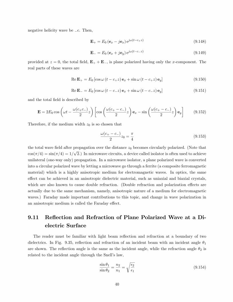
negative helicity wave be �c. Then,

E+ = E0 (ex � jex) ej!(t�c+z) (9.148)

E� = E0 (ex + jey) ej!(t�c�z) (9.149)

provided at z = 0, the total �eld, E+ +E�, is plane polarized having only the x-component. The

real parts of these waves are

ReE+ = E0 [cos! (t� c+z) ex + sin! (t� c+z) ey] (9.150)

ReE� = E0 [cos! (t� c�z) ex + sin! (t� c�z) ey] (9.151)

and the total �eld is described by

E = 2E0 cos

�!t� !(c+c�)

2z

��cos

�!(c+ � c�)

2z

�ex � sin

�!(c+ � c�)

2z

�ey

�(9.152)

Therefore, if the medium width z0 is so chosen that

!(c+ � c�)2

z0 =�

4(9.153)

the total wave �eld after propagation over the distance z0 becomes circularly polarized. (Note that

cos(�=4) = sin(�=4) = 1=p2.) In microwave circuits, a device called isolator is often used to achieve

unilateral (one-way only) propagation. In a microwave isolator, a plane polarized wave is converted

into a circular polarized wave by letting a microwave go through a ferrite (a composite ferromagnetic

material) which is a highly anisotropic medium for electromagnetic waves. In optics, the same

e¤ect can be achieved in an anisotropic dielectric material, such as uniaxial and biaxial crystals,

which are also known to cause double refraction. (Double refraction and polarization e¤ects are

actually due to the same mechanism, namely, anisotropic nature of a medium for electromagnetic

waves.) Faraday made important contributions to this topic, and change in wave polarization in

an anisotropic medium is called the Faraday e¤ect.

9.11 Re�ection and Refraction of Plane Polarized Wave at a Di-electric Surface

The reader must be familiar with light beam re�ection and refraction at a boundary of two

dielectrics. In Fig. 9.35, re�ection and refraction of an incident beam with an incident angle �1are shown. The re�ection angle is the same as the incident angle, while the refraction angle �2 is

related to the incident angle through the Snell�s law,

sin �1sin �2

=n2n1=

r�2�1

(9.154)

40

where ni is the index of refraction de�ned by

ni =c

ci=

r�i�0

(9.155)

with �i the permittivity of the respective medium. Strictly speaking, re�ection and refraction should

be analyzed by incorporating appropriate boundary conditions for the electric and magnetic �elds

at the dielectric boundary. Since no free charges and conduction currents are present, the boundary

conditions are

Et1 = Et2; Ht1 = Ht2; Dn1 = Dn2; Bn1 = Bn2 (9.156)

where �t� is for tangential components, and �n� for normal components. The wave velocities in

each medium are

c1 =!

k1; c2 =

!

k2(9.157)

with the vectors k1 and k2 being along the beam direction in each medium. Let us �rst consider the

case of electric �eld polarization parallel to the boundary surface shown in Fig. 9.20 (top �gure).

We denote the incident electric �eld by E0, re�ected �eld by E1, and refracted �eld by E2. Since

all of these �elds are tangential to the boundary, we have

E0 + E1 = E2 (9.158)

The magnetic �elds associated with the electric �elds are to be found from Maxwell�s equation

r�E = ��0@H

@t(9.159)

For plane waves, this reduces to

k�E =!�0H (9.160)

In the medium �1,!

k1=

1p�1�0

(9.161)

and in the medium �2,!

k2=

1p�2�0

(9.162)

The tangential magnetic �eld associated with the incident wave is given by

H0t =k1!�0

E0 cos �1 (9.163)

the re�ected magnetic �eld is

H1t =k1!�0

E1 cos �1 (9.164)

41

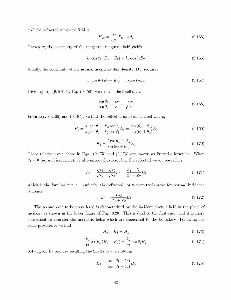
and the refracted magnetic �eld is

H2t =k2!�0

E2 cos �2 (9.165)

Therefore, the continuity of the tangential magnetic �eld yields

k1 cos �1 (E0 � E1) = k2 cos �2E2 (9.166)

Finally, the continuity of the normal magnetix �ux density, Bn, requires

k1 cos �1(E0 + E1) = k2 cos �2E2 (9.167)

Dividing Eq. (9.167) by Eq. (9.158), we recover the Snell�s law

sin �1sin �2

=k2k1=

r�2�1

(9.168)

From Eqs. (9.166) and (9.167), we �nd the re�ected and transmitted waves,

E1 =k1 cos �1 � k2 cos �2k1 cos �1 � k2 cos �2

E0 =sin (�2 � �1)sin (�2 + �1)

E0 (9.169)

E2 =2 cos �1 sin �2sin (�2 + �1)

E0 (9.170)

These relations and those in Eqs. (9.175) and (9.176) are known as Fresnel�s formulae. When

�1 = 0 (normal incidence), �2 also approaches zero, but the re�ected wave approaches

E1 =

p�1 �

p�2p

�2 +p�1E0 =

Z2 � Z1Z1 + Z2

E0 (9.171)

which is the familiar result. Similarly, the refracted (or transmitted) wave for normal incidence

becomes

E2 =2Z2

Z1 + Z2E0 (9.172)

The second case to be considered is characterized by the incident electric �eld in the plane of

incident as shown in the lower �gure of Fig. 9.20. This is dual to the �rst case, and it is more

convenient to consider the magnetic �elds which are tangential to the boundary. Following the

same procedure, we �nd

H0 +H1 = H2 (9.173)

k1�1cos �1 (H0 �H1) =

k2�2cos �2H2 (9.174)

Solving for H1 and H2 recalling the Snell�s law, we obtain

H1 =tan (�1 � �2)tan (�1 + �2)

H0 (9.175)

42

H2 =sin 2�1

sin (�1 + �2) cos (�1 � �2)H0 (9.176)

The re�ected wave H1 vanishes when

�1 + �2 =�

2or �1 =

�

2� �2 (9.177)

At this particular incident angle, the Snell�s law becomes

sin �1sin �2

=sin �1

cos��2� �1

� = tan �1 =r�2�1=n2n1

(9.178)

This special angle at which re�ection can be avoided is called the Brewster angle and is often

exploited in optical design to minimize light re�ection. Note that null re�ection can occur only

when the incident electric �eld is so polarized that the �eld is in the incident plane. If glass has an

index of refraction n = 1:5; (� = 2:25�0), the Brewster�s angle becomes �B = tan�1(1:5) = 56:3�.

43

θ θ

θ

1 1

2

θ θ

θ

1 1

2

H H

H

H H

H

E E

E

E

E E

εε1

2

ε1

ε2

i

i r

r

i

i r

r

t

t

t

t

Figure 9-22: Re�ection and refraction at a dielectric boundary. (a) The magnetic �eld in theincident plane. (b) The electric �eld in the incident plane.

44