Time Series

Math 419/592

Winter 2009

Prof. Andrew Ross

Eastern Michigan University

Overview of Stochastic Models

No Space Discrete ContinuousNo Time Ch 1, 2, 3 Ch 1, 2, 3Discrete Ch 4 DTMC YOU ARE HEREContinuous Ch 5, 7 Ch 5, 6, 7, 8 Ch 10

Or, if you prefer,transpose it:

No Time Discrete ContinuousNo Space Ch 5, 7Discrete Ch 1, 2, 3 Ch 4 DTMC Ch 5, 6, 7, 8Continuous Ch 1, 2, 3 YOU ARE HERE Ch 10

But first, a word from our sponsor

Take Math 560(Optimization)

this fall!

Sign up soon or it will disappear

Outline

Look at the data! Common Models Multivariate Data Cycles/Seasonality Filters

Look at the data!

or else!

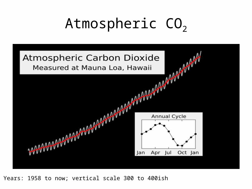
Atmospheric CO2

Years: 1958 to now; vertical scale 300 to 400ish

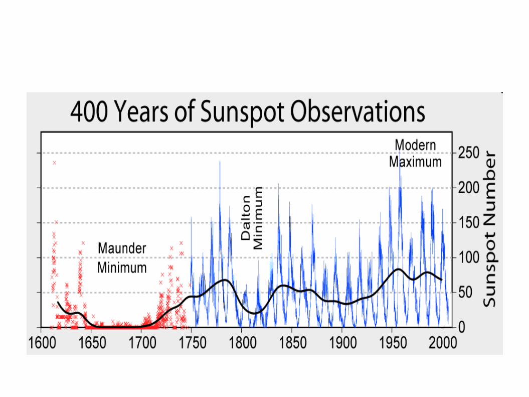
Ancient sunspot data

Our Basic Procedure

1. Look at the data

2. Quantify any pattern you see

3. Remove the pattern

4. Look at the residuals

5. Repeat at step 2 until no patterns left

Our basic procedure, version 2.0

Look at the data Suck the life out of it Spend hours poring over the noise

What should noise look like?

One of these things is not like the others

0 10 20 30 40 50 60 70

0

1

2

3

4

5

6

7

0 10 20 30 40 50 60 70

-1.5

-1

-0.5

0

0.5

1

1.5

2

0 10 20 30 40 50 60 70

-1.5

-1

-0.5

0

0.5

1

1.5

2

2.5

0 10 20 30 40 50 60 70

-0.3

-0.2

-0.1

0

0.1

0.2

0.3

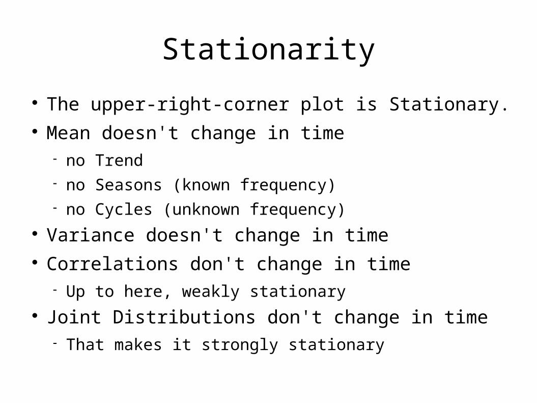
Stationarity

The upper-right-corner plot is Stationary. Mean doesn't change in time

no Trend no Seasons (known frequency) no Cycles (unknown frequency)

Variance doesn't change in time Correlations don't change in time

Up to here, weakly stationary Joint Distributions don't change in time

That makes it strongly stationary

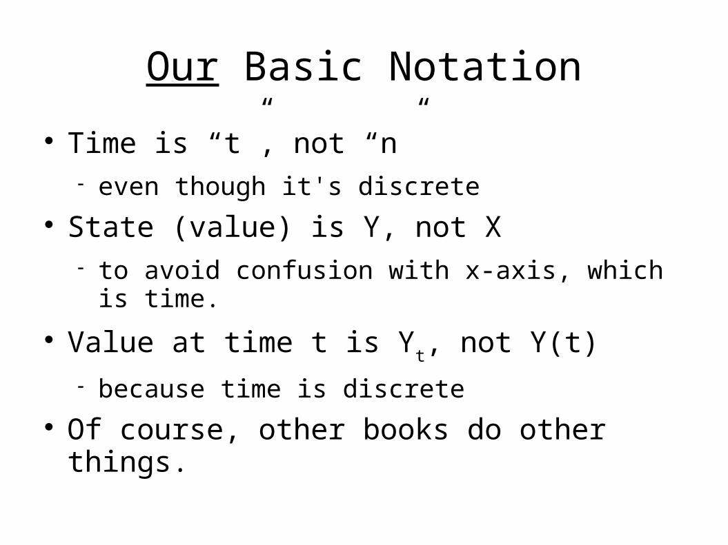
Our Basic Notation

Time is “t”, not “n” even though it's discrete

State (value) is Y, not X to avoid confusion with x-axis, which is time.

Value at time t is Yt, not Y(t)

because time is discrete Of course, other books do other things.

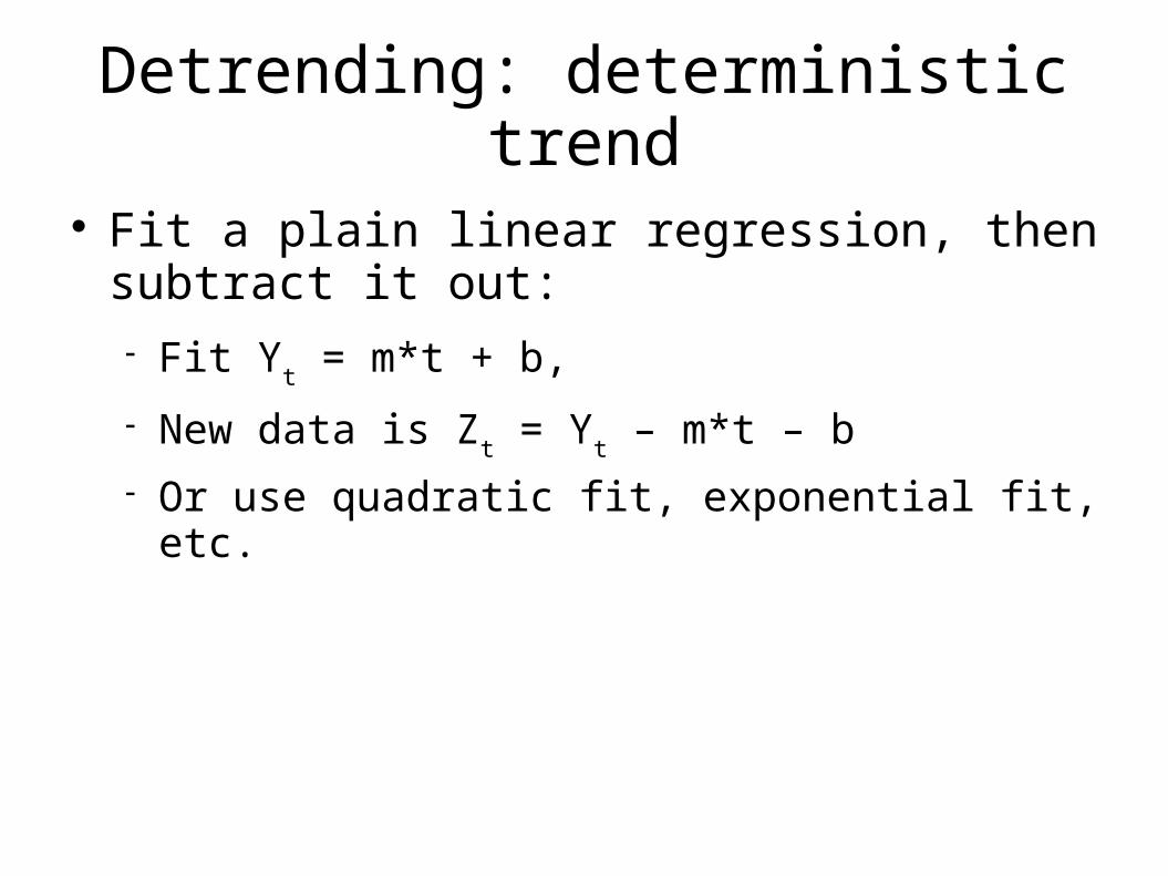
Detrending: deterministic trend

Fit a plain linear regression, then subtract it out: Fit Y

t = m*t + b,

New data is Zt = Y

t – m*t – b

Or use quadratic fit, exponential fit, etc.

Detrending: stochastic trend

Differencing For linear trend, new data is Z

t = Y

t – Y

t-1 To remove quadratic trend, do it again:

Wt = Z

t – Z

t-1=Y

t – 2Y

t-1 + Y

t-2 Like taking derivatives

What’s the equivalent if you think the trend is exponential, not linear?

Hard to decide: regression or differencing?

Removing Cycles/Seasons

Will get to it later.

For the next few slides, assume no cycles/seasons.

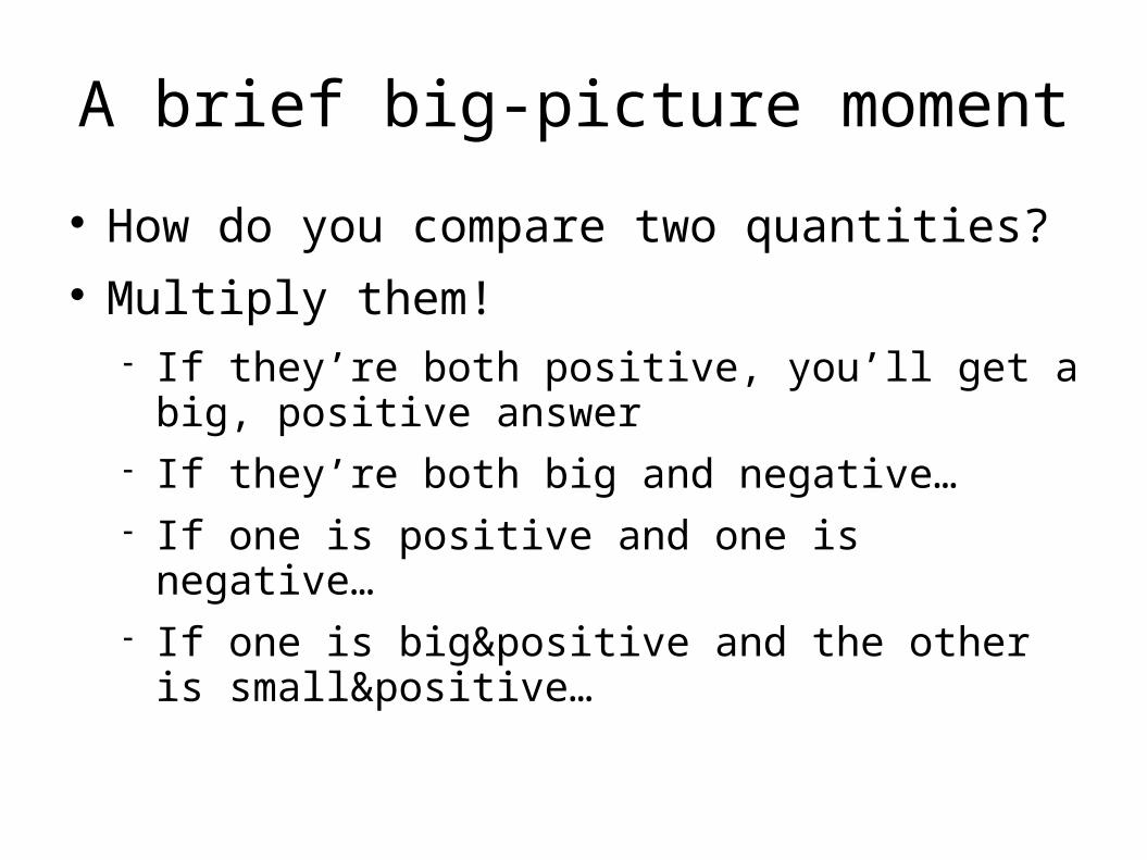
A brief big-picture moment

How do you compare two quantities? Multiply them!

If they’re both positive, you’ll get a big, positive answer

If they’re both big and negative… If one is positive and one is negative… If one is big&positive and the other is

small&positive…

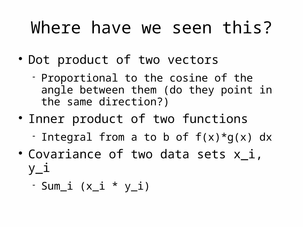
Where have we seen this?

Dot product of two vectors Proportional to the cosine of the angle between

them (do they point in the same direction?) Inner product of two functions

Integral from a to b of f(x)*g(x) dx Covariance of two data sets x_i, y_i

Sum_i (x_i * y_i)

Autocorrelation Function

How correlated is the series with itself at various lag values?

E.g. If you plot Yt+1

versus Yt and find the

correlation, that's the correl. at lag 1 ACF lets you calculate all these correls. without

plotting at each lag value. ACF is a basic building block of time series

analysis.

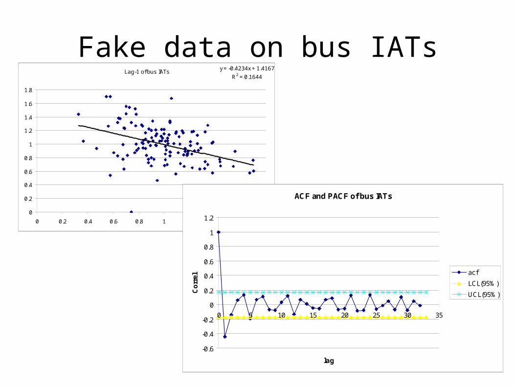
Fake data on bus IATsLag-1 of bus IATs

y = -0.4234x + 1.4167

R2 = 0.1644

0

0.2

0.4

0.6

0.8

1

1.2

1.4

1.6

1.8

0 0.2 0.4 0.6 0.8 1 1.2 1.4 1.6 1.8

ACF and PACF of bus IATs

-0.6

-0.4

-0.2

0

0.2

0.4

0.6

0.8

1

1.2

0 5 10 15 20 25 30 35

lag

Co

rrel

acf

LCL(95%)

UCL(95%)

Properties of ACF

At lag 0, ACF=1 Symmetric around lag 0 Approx. confidence-interval bars around ACF=0

To help you decide when ACF drops to near-0 Less reliable at higher lags Often assume ACF dies off fast enough so its

absolute sum is finite. If not, called “long-term memory”; e.g.

River flow data over many decades Traffic on computer networks

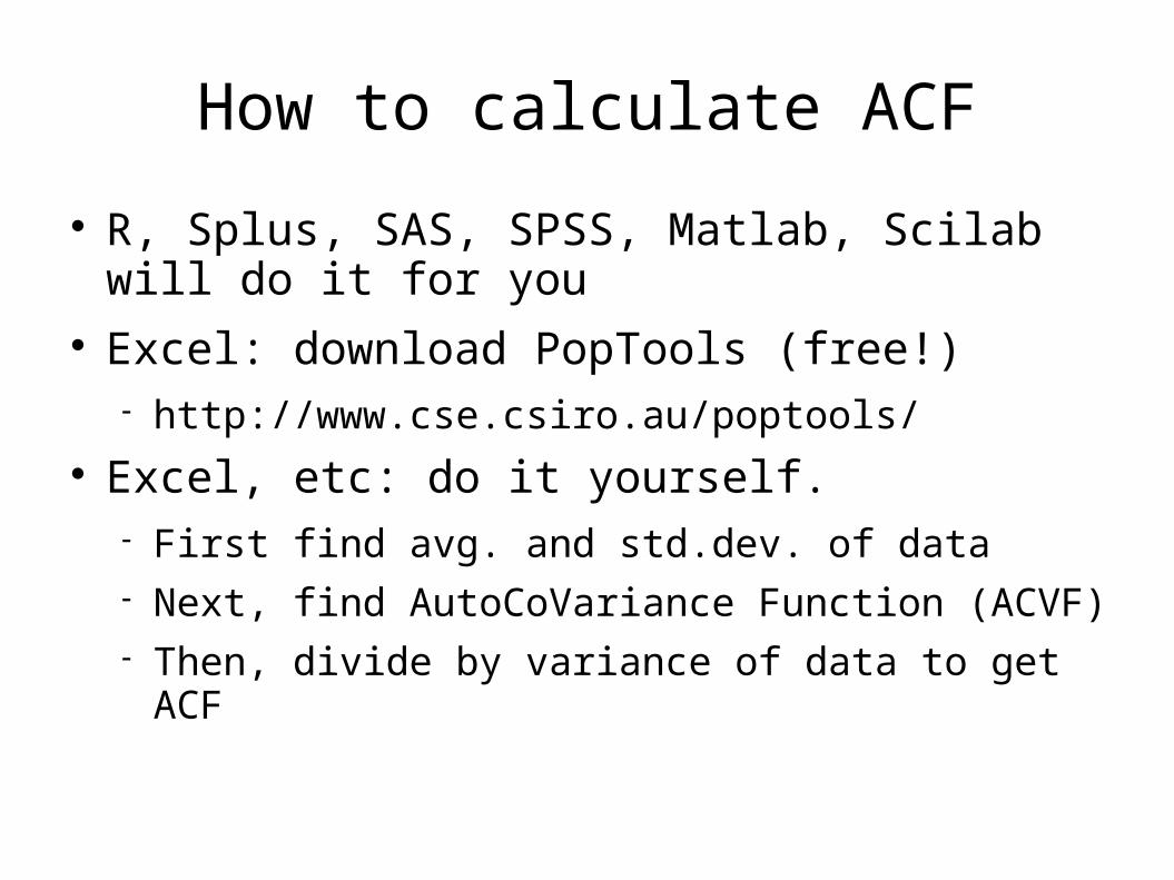
How to calculate ACF

R, Splus, SAS, SPSS, Matlab, Scilab will do it for you

Excel: download PopTools (free!) http://www.cse.csiro.au/poptools/

Excel, etc: do it yourself. First find avg. and std.dev. of data Next, find AutoCoVariance Function (ACVF) Then, divide by variance of data to get ACF

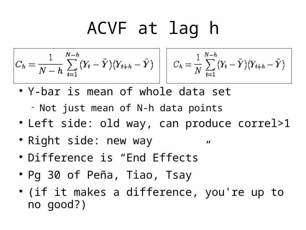
ACVF at lag h

Y-bar is mean of whole data set Not just mean of N-h data points

Left side: old way, can produce correl>1 Right side: new way Difference is “End Effects” Pg 30 of Peña, Tiao, Tsay (if it makes a difference, you're up to no good?)

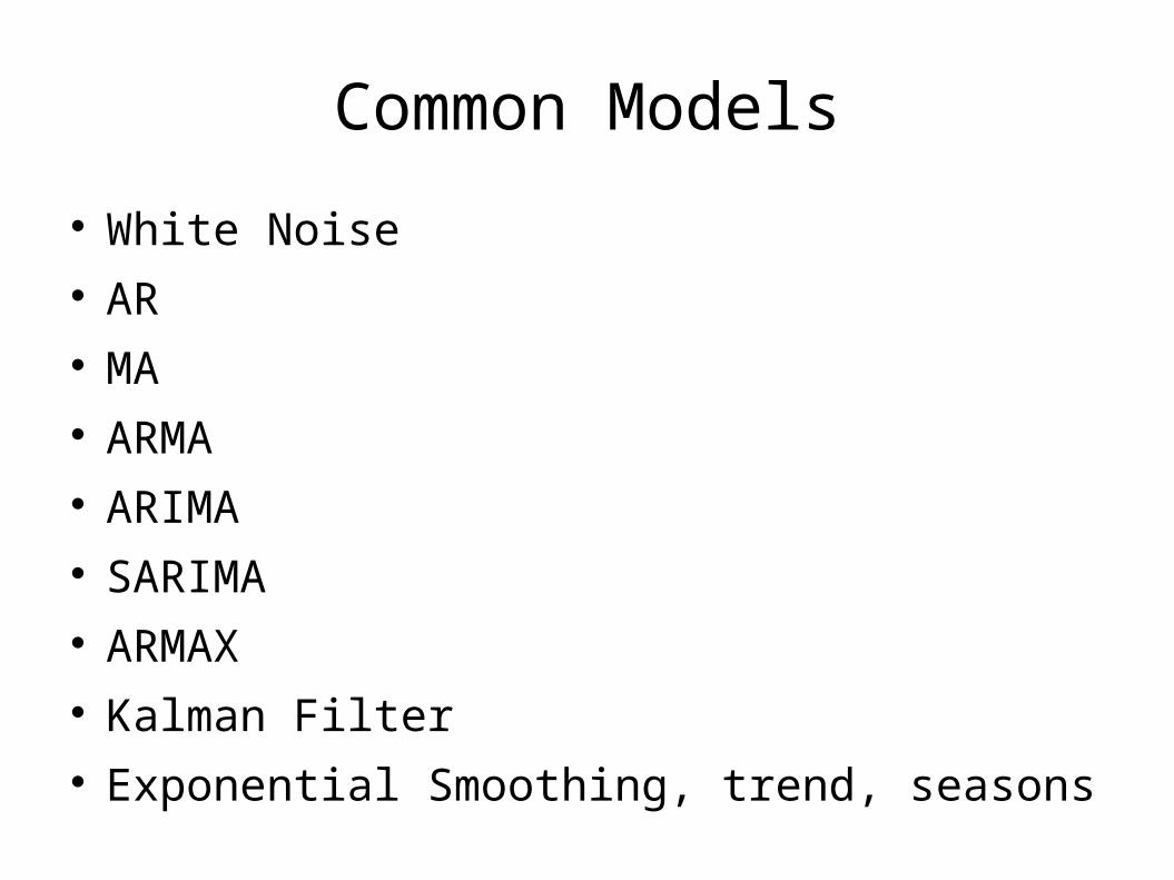
Common Models

White Noise AR MA ARMA ARIMA SARIMA ARMAX Kalman Filter Exponential Smoothing, trend, seasons

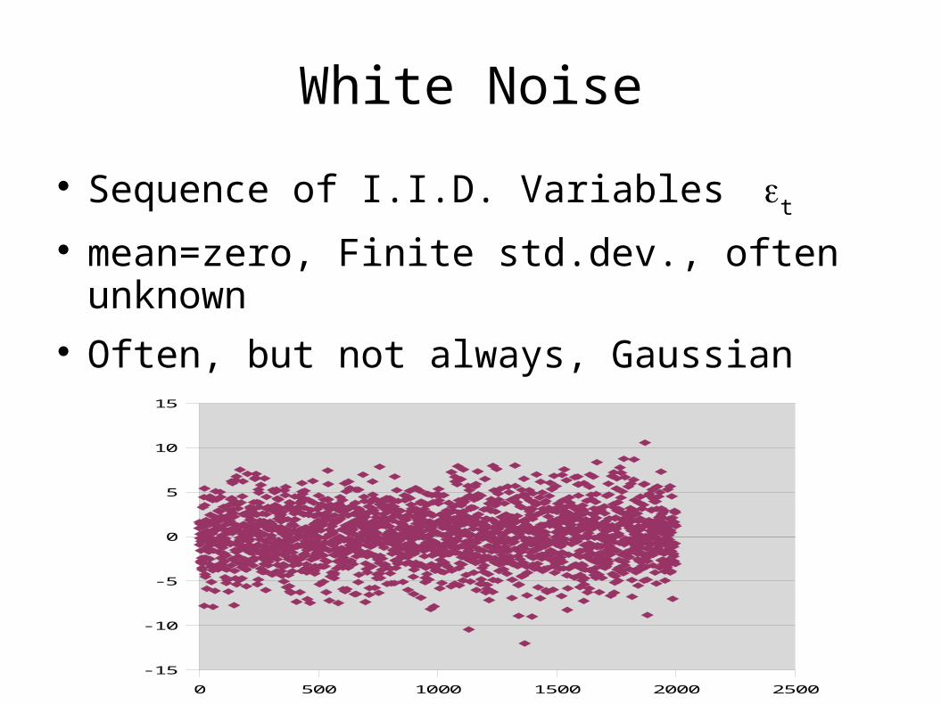
White Noise

Sequence of I.I.D. Variablest

mean=zero, Finite std.dev., often unknown Often, but not always, Gaussian

0 500 1000 1500 2000 2500

-15

-10

-5

0

5

10

15

AR: AutoRegressive

Order 1: Yt=a*Y

t-1 +

t

E.g. New = (90% of old) + random fluctuation

Order 2: Yt=a

1*Y

t-1 +a

2*Y

t-2+

t

Order p denoted AR(p) p=1,2 common; >2 rare AR(p) like p'th order ODE AR(1) not stationary if |a|>=1 E[Y

t] = 0, can generalize

Things to do with AR

Find appropriate order Estimate coefficients

via Yule-Walker eqn. Estimate std.dev. of white noise If estimated |a|>0.98, try differencing.

MA: Moving Average

Order 1:

Yt = b

0

t +b

1

t-1

Order q: MA(q) In real data, much less common than AR But still important in theory of filters Stationary regardless of b values E[Y

t] = 0, can generalize

ACF of an MA process

Drops to zero after lag=q

That's a good way to determine what q should be!

A CF

-1

-0.8

-0.6

-0.4

-0.2

0

0.2

0.4

0.6

0.8

1

0 5 10 15 20 25 30

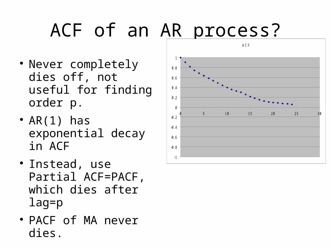
ACF of an AR process?

Never completely dies off, not useful for finding order p.

AR(1) has exponential decay in ACF

Instead, use Partial ACF=PACF, which dies after lag=p

PACF of MA never dies.

A CF

-1

-0.8

-0.6

-0.4

-0.2

0

0.2

0.4

0.6

0.8

1

0 5 10 15 20 25 30

ARMA

ARMA(p,q) combines AR and MA Often p,q <= 1 or 2

ARIMA

AR-Integrated-MA ARIMA(p,d,q) d=order of differencing before applying

ARMA(p,q) For nonstationary data w/stochastic trend

SARIMA, ARMAX

Seasonal ARIMA(p,d,q)-and-(P,D,Q)S

Often S= 12 (monthly) or 4 (quarterly) or 52 (weekly)

Or, S=7 for daily data inside a week

ARMAX=ARMA with outside explanatory variables (halfway to multivariate time series)

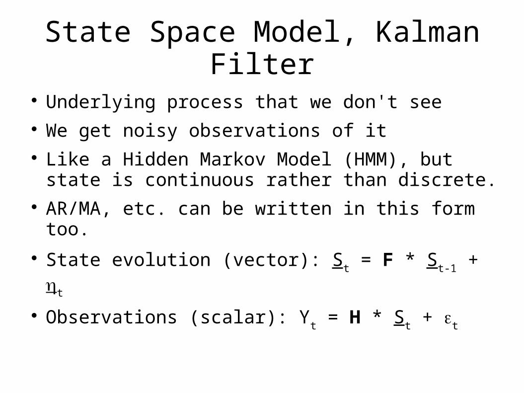
State Space Model, Kalman Filter

Underlying process that we don't see We get noisy observations of it Like a Hidden Markov Model (HMM), but state

is continuous rather than discrete. AR/MA, etc. can be written in this form too. State evolution (vector): S

t = F * S

t-1 +

t

Observations (scalar): Yt = H * S

t +

t

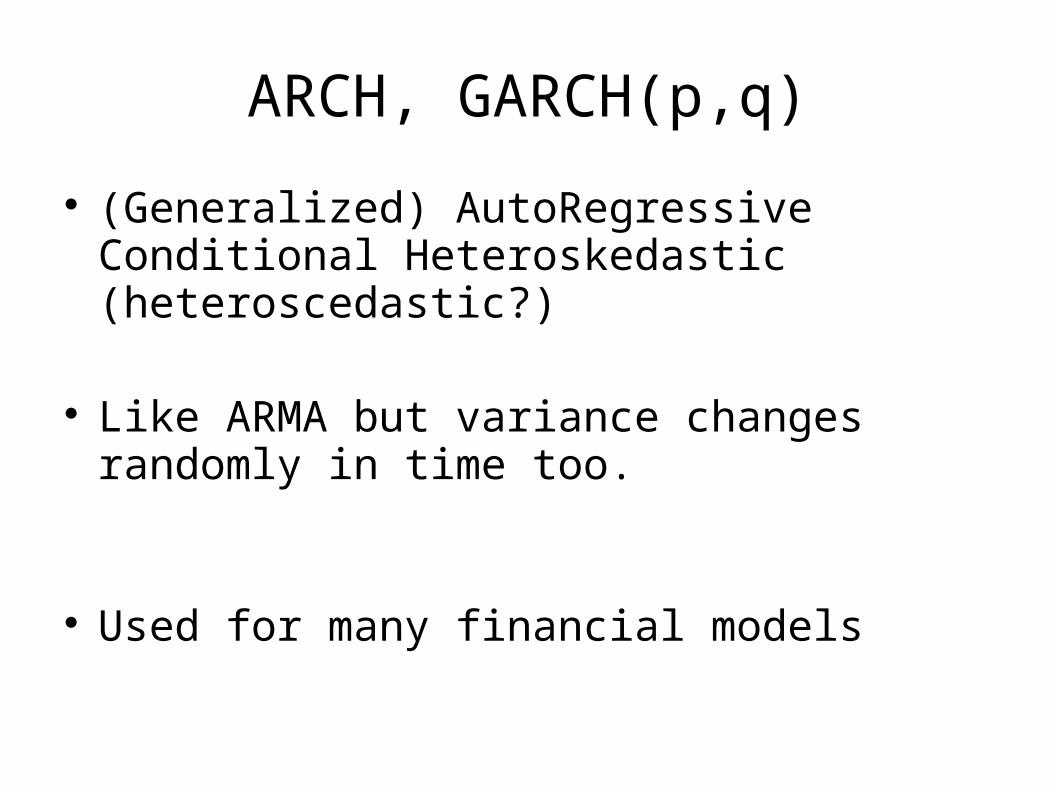
ARCH, GARCH(p,q)

(Generalized) AutoRegressive Conditional Heteroskedastic (heteroscedastic?)

Like ARMA but variance changes randomly in time too.

Used for many financial models

Exponential Smoothing

More a method than a model.

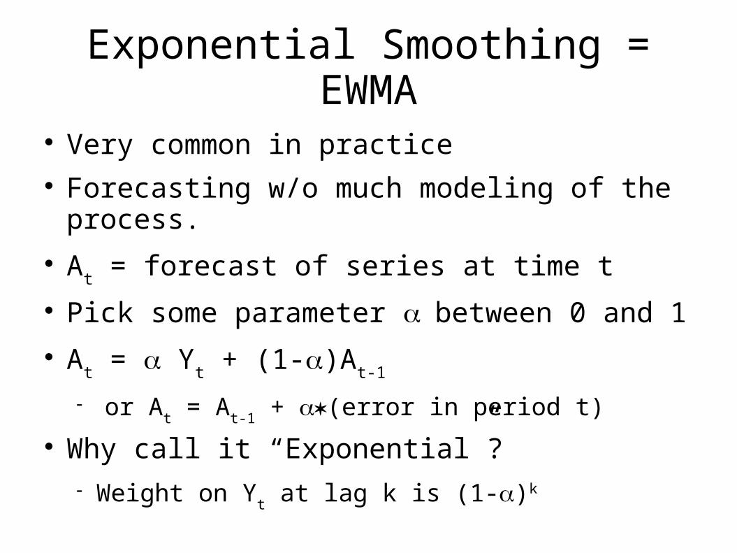
Exponential Smoothing = EWMA

Very common in practice Forecasting w/o much modeling of the process. A

t = forecast of series at time t

Pick some parameter between 0 and 1 A

t = Y

t + (1-)A

t-1

or A

t = A

t-1 + (error in period t)

Why call it “Exponential”? Weight on Y

t at lag k is (1-)k

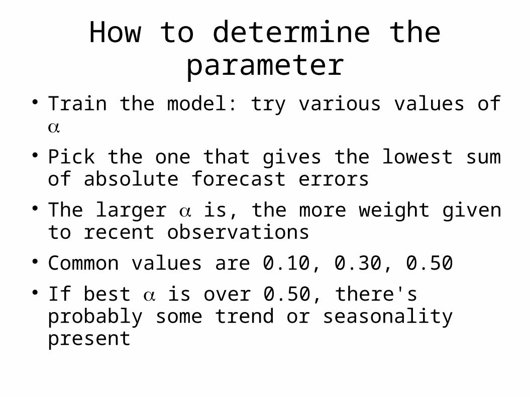
How to determine the parameter

Train the model: try various values of Pick the one that gives the lowest sum of

absolute forecast errors The larger is, the more weight given to recent

observations Common values are 0.10, 0.30, 0.50 If best is over 0.50, there's probably some

trend or seasonality present

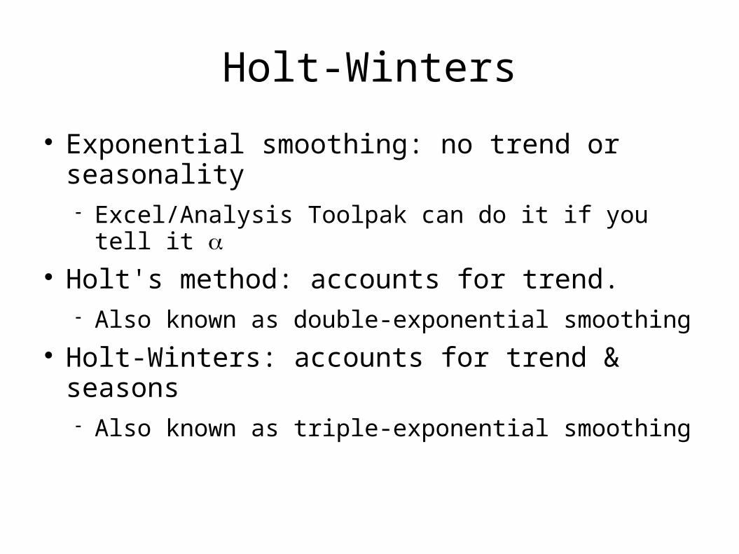
Holt-Winters

Exponential smoothing: no trend or seasonality Excel/Analysis Toolpak can do it if you tell it

Holt's method: accounts for trend. Also known as double-exponential smoothing

Holt-Winters: accounts for trend & seasons Also known as triple-exponential smoothing

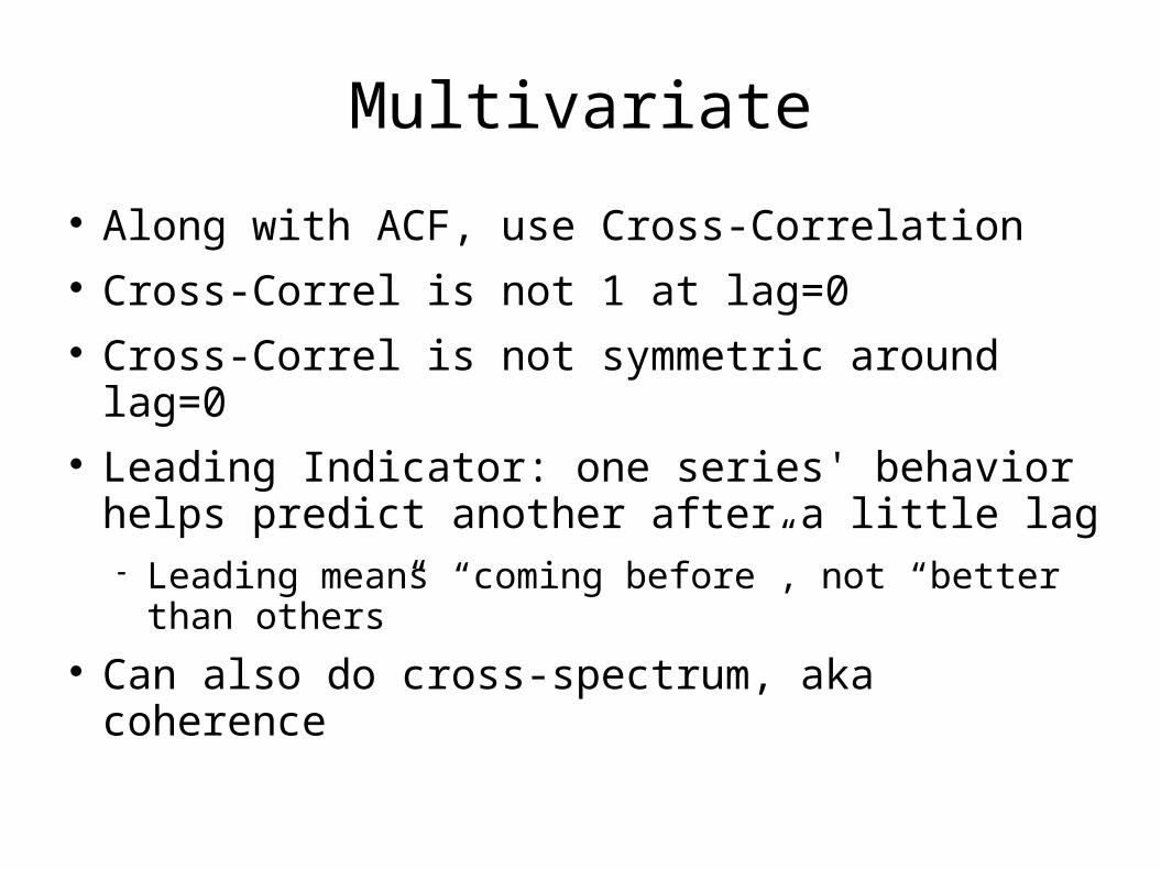
Multivariate

Along with ACF, use Cross-Correlation Cross-Correl is not 1 at lag=0 Cross-Correl is not symmetric around lag=0 Leading Indicator: one series' behavior helps

predict another after a little lag Leading means “coming before”, not “better than

others” Can also do cross-spectrum, aka coherence

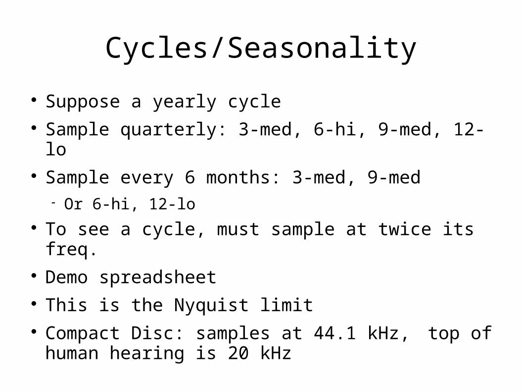
Cycles/Seasonality

Suppose a yearly cycle Sample quarterly: 3-med, 6-hi, 9-med, 12-lo Sample every 6 months: 3-med, 9-med

Or 6-hi, 12-lo To see a cycle, must sample at twice its freq. Demo spreadsheet This is the Nyquist limit Compact Disc: samples at 44.1 kHz,

top of human hearing is 20 kHz

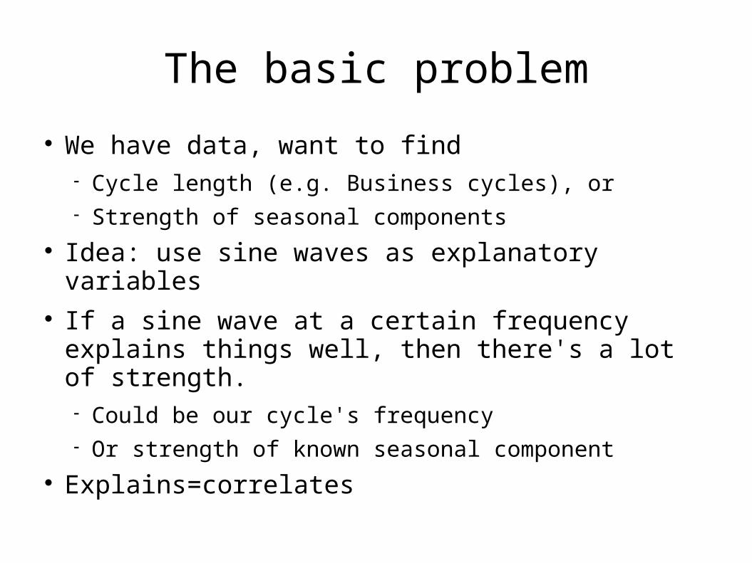
The basic problem

We have data, want to find Cycle length (e.g. Business cycles), or Strength of seasonal components

Idea: use sine waves as explanatory variables If a sine wave at a certain frequency explains

things well, then there's a lot of strength. Could be our cycle's frequency Or strength of known seasonal component

Explains=correlates

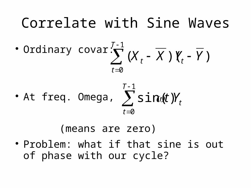
Correlate with Sine Waves

Ordinary covar:

At freq. Omega,

(means are zero) Problem: what if that sine is out of phase with

our cycle?

1

0

))((T

ttt YYXX

1

0

)sin(T

ttYt

Solution

Also correlate with a cosine 90 degrees out of phase with sine

Why not also with a 180-out-of-phase? Because if that had a strong correl, our original sine

would have a strong correl of opposite sign. Sines & Cosines, Oh My—combine using

complex variables!

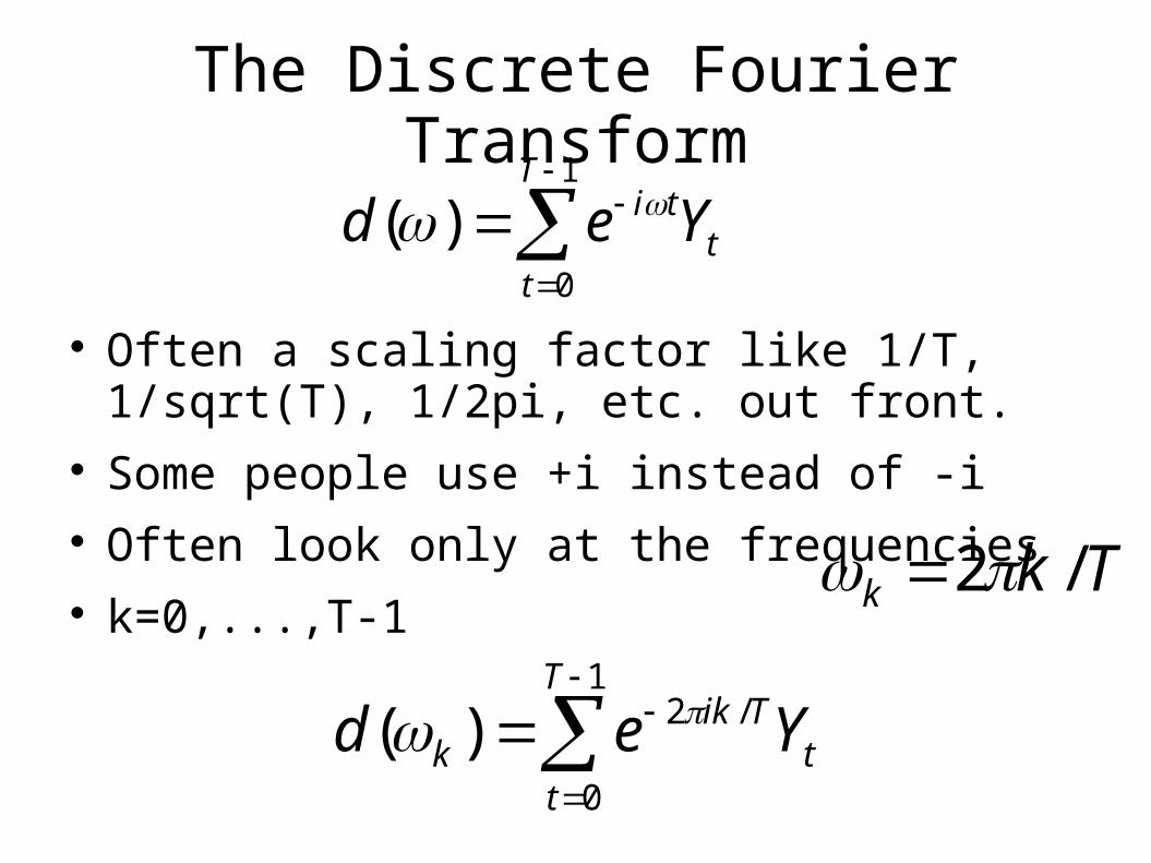
The Discrete Fourier Transform

Often a scaling factor like 1/T, 1/sqrt(T), 1/2pi, etc. out front.

Some people use +i instead of -i Often look only at the frequencies k=0,...,T-1

1

0

)(T

tt

ti Yed

Tkk /2

1

0

/2)(T

tt

Tikk Yed

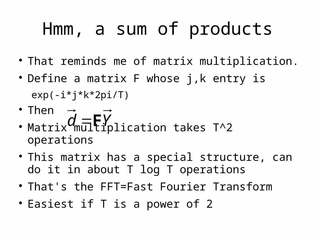
Hmm, a sum of products

That reminds me of matrix multiplication. Define a matrix F whose j,k entry is

exp(-i*j*k*2pi/T) Then Matrix multiplication takes T^2 operations This matrix has a special structure, can do it in

about T log T operations That's the FFT=Fast Fourier Transform Easiest if T is a power of 2

Yd F

So now we have complex values...

Take magnitude & argument of each DFT result Plot squared magnitude vs. frequency

This is the “Periodogram” Large value = that frequency is very strong Often plotted on semilog-y scale, “decibels” Example spreadsheet

Spreadsheet Experiments

First, play with amplitudes: (1,0) then (0,1) then (1,.5) then (1,.7)

Next, play with frequency1: 2*pi/8 then 2*pi/4 2*pi/6, 2*pi/7, 2*pi/9, 2*pi/10 2*pi/100, 2*pi/1000 Summarize your results for yourself. Write it down!

Reset to 2*pi/8 then play with phase2: 0, 1, 2, 3, 4, 5, 6...

Now add some noise to Yt

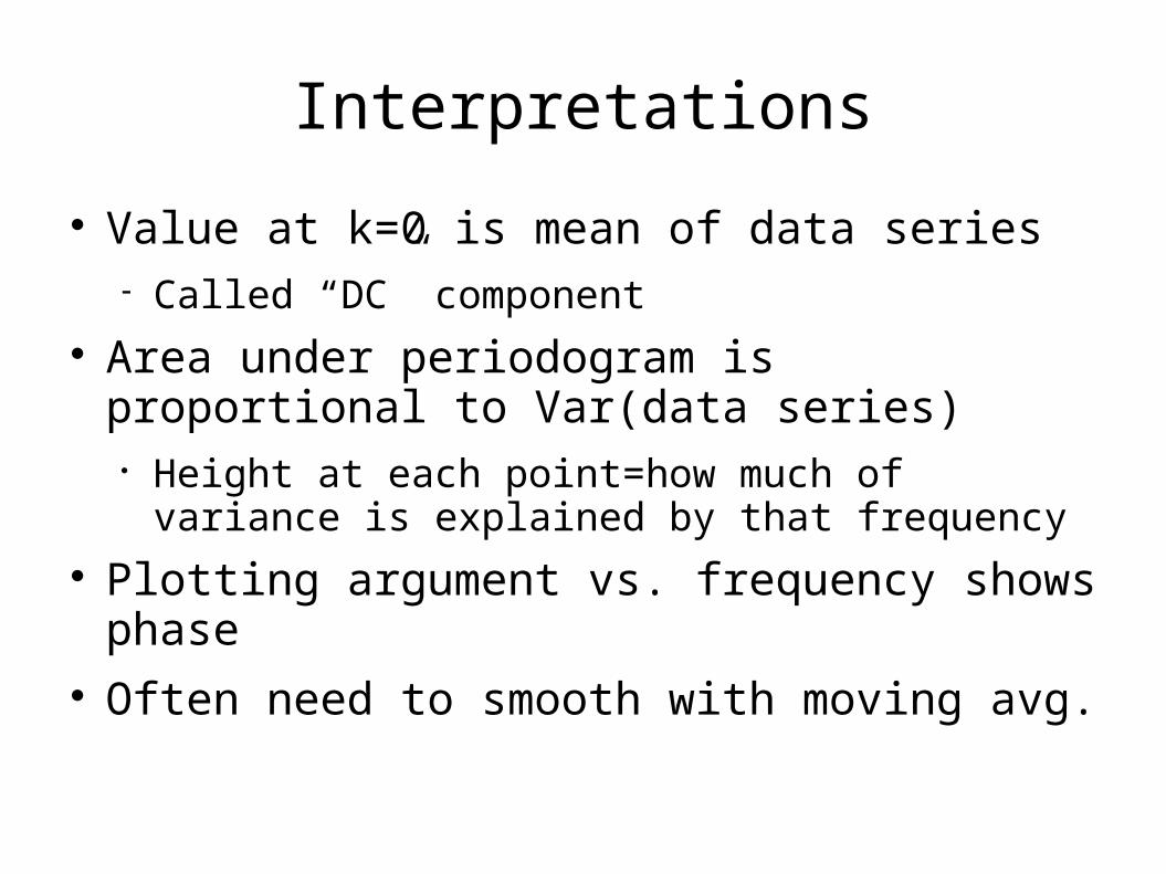
Interpretations

Value at k=0 is mean of data series Called “DC” component

Area under periodogram is proportional to Var(data series)

Height at each point=how much of variance is explained by that frequency

Plotting argument vs. frequency shows phase Often need to smooth with moving avg.

What is FT of White Noise?

Try it! Why is it called white noise? Pink noise, etc. (look up in Wikipedia)

Filtering: part 1

Zero out the frequencies you don't want Invert the FT

FT is its own inverse! Not like Laplace Transform. This is “frequency-domain” filtering MP3 files: filter out the freqs. you wouldn't hear

because they're overwhelmed by stronger frequencies

Filtering: part 2

Time-domain filtering: example spreadsheet Smoothing: moving average

Filters out high frequencies (noise is high-freq) Low-pass filter

Detrending: differencing Filters out trends and slow cycles (which look like

trends, locally) High-pass filter

Band-pass filter Band-reject filter (esp. 12-month cycles)

Filtering

Time-domain filter's freq. response comes from the FT of its averaging coefficients

Example spreadsheet This curve is called the “Transfer Function” Good audio speakers publish their frequency

response curves

Long-history time series

Ordinary theory assumes that ACF dies off faster than 1/h

But some time series don't satisfy that: River flows Packet amounts on data networks

Connected to chaos & fractals

Bibliography

Enders: Applied Econometric Time Series Kedem & Fokianos: Regression Models for Time

Series Analysis Pen~a, Tao, Tsay: A Course in Time Series Analysis Brillinger: lecture notes for Stat 248 at UC Berkeley Brillinger:Time Series: Data Analysis and Theory Brockwell & Davis: Introduction to Time Series and

Forecasting

1 real way, 2 fake ways:

0 10 20 30 40 50 60 70

-0.3

-0.2

-0.1

0

0.1

0.2

0.3