time scales and spatial patterns of passive ocean

Time Scales and Spatial Patterns of Passive Ocean–Atmosphere Decay Modes*BENJAMIN R. LINTNER AND J. DAVID NEELIN

Department of Atmospheric and Oceanic Sciences, and Institute of Geophysics and Planetary Physics, University of California,Los Angeles, Los Angeles, California

(Manuscript received 23 February 2007, in final form 7 September 2007)

ABSTRACT

The decay characteristics of a mixed layer ocean passively coupled to an atmospheric model are impor-tant to the response of the climate system to stochastic or external forcing. Two salient features of suchdecay—the spatial-scale dependence of sea surface temperature anomaly (SSTA) decay time scales and thespatial inhomogeneities of SSTA decay modes—are addressed using intermediate-level complexity andsimple analytic models of the tropical atmosphere. As expected, decay time scales increase with the spatialextent of the SSTA. Most modes decay rapidly—with characteristic decay times of 50–100 days for a 50-mmixed layer—with the decay determined by local surface flux adjustment. Only those modes with spatialscales approaching or larger than the tropical basin scale exhibit decay time scales distinctively longer thanthe local decay, with the decay time scale of the most slowly decaying mode of the order of 250–300 daysin the tropics (500 days globally). Simple analytic prototypes of the spatial-scale dependence and the effectof basic-state inhomogeneities, especially the impact of nonconvecting regions, elucidate these results.Horizontal energy transport sets the transition between fast, essentially local, decay time scales and theslower decay at larger spatial scales; within the tropics, efficient wave dynamics accounts for the smallnumber of slowly decaying modes. Inhomogeneities in the basic-state climate, such as the presence orabsence of mean tropical deep convection, strongly impact large-scale SSTA decay characteristics. Fornonconvecting regions, SSTA decay is slow because evaporation is limited by relatively slow moisturedivergence. The separation of convecting- and nonconvecting-region decay times and the closeness of theslower nonconvecting-region decay time scale to the most slowly decaying modes cause a blending betweenlocal nonconvecting modes and the large-scale modes, resulting in pronounced spatial inhomogeneity in theslow decay modes.

1. Introduction

Coupling of the ocean–atmosphere system is an im-portant facet of climate system variability relevant toadjustment processes and teleconnections. It is concep-tually useful to distinguish the following two types ofocean–atmosphere coupling: “active” and “passive.”The former involves changes to ocean circulation (e.g.,surface wind stress forcing or thermocline dynamics)that impact surface temperatures and feedback to theatmosphere. Active coupling plays a crucial role in theevolution and dynamics of El Niño–Southern Oscilla-

tion (ENSO; Philander et al. 1984; Cane and Zebiak1986; Battisti 1988; Neelin et al. 1998; and referencestherein), as interactions of the thermocline, equatorialocean wave dynamics, surface fluxes, and convectiondictate the spatial extent and time scales of ENSOevents. Active coupling has been further implicated inthe low-frequency variability of the extratropical seasurface temperature anomalies (SSTAs), with oceanicRossby wave dynamics and the thermohaline and wind-driven circulations contributing to the development ofspatially coherent modes of SSTA variability on inter-decadal and longer time scales (Münnich et al. 1998;Neelin and Weng 1999; Gallego and Cessi 2001; Mar-shall et al. 2001).

Passive ocean–atmosphere coupling is simpler, as itinvolves only thermodynamically mediated changes toocean heat storage. For a net surface flux FNET � E �H � RS, where E is latent heating (evaporation), H issensible heating, and RS is the net surface longwaveplus shortwave radiative heating, the time evolution ofa passively coupled mixed layer is simply

* Institute of Geophysics and Planetary Physics ContributionNumber 6310.

Corresponding author address: Dr. Benjamin R. Lintner, De-partment of Atmospheric and Oceanic Sciences, University ofCalifornia, Los Angeles, 405 Hilgard Ave., 7127 Math ScienceBldg., Los Angeles, CA 90095-1565.E-mail: [email protected]

15 MAY 2008 L I N T N E R A N D N E E L I N 2187

DOI: 10.1175/2007JCLI1913.1

© 2008 American Meteorological Society

JCLI1913

cM�tTs � FNET, �1�

where TS is the mixed layer temperature and cM is themixed layer heat capacity. The use of passive couplingis well known from studies of the extratropical SSTresponse to short time-scale atmospheric forcing (Has-selmann 1976; Frankignoul and Hasselmann 1977; Bar-sugli and Battisti 1998). In the simple stochastic modelsof Hasselmann (1976) and Frankignoul and Hassel-mann (1977), FNET is just

FNET � ��Ts

netTs � �, �2�

where the first term on the right-hand side is the neteffect of (negative) surface heat flux feedbacks; that is,�net

Ts(�0) is a damping coefficient representing the net

surface heat flux anomaly per unit Ts anomaly and � isthe net heat flux associated with stochastic “weathernoise” forcing.

In the tropics, passive coupling also plays a signifi-cant role, especially in the context of tropical telecon-nections (Klein et al. 1999; Saravanan and Chang 2000).The thermal inertia of the ocean mixed layer delays theremote surface temperature response to El Niño, whichin turn impacts tropospheric warming and precipitation(see, e.g., Chang et al. 1998; Alexander et al. 2002; Gi-annini et al. 2001; Chiang and Sobel 2002; Tang andNeelin 2004; Neelin and Su 2005; Su et al. 2005, here-after SNM05; Chiang and Lintner 2005). Studies ofother coupled tropical phenomena, including intrasea-sonal variability and the Madden–Julian oscillation,further demonstrate the potential impacts of passivecoupling (Sobel and Gildor 2003; Maloney and Sobel2004; Grabowski 2006; Zhang et al. 2006). Passive cou-pling also modulates the transient response to globalwarming (Chou and Neelin 2004; Chou et al. 2006).

The form of FNET in (2) is reasonable for the mid-latitudes, where the effect of surface fluxes on the at-mosphere may be neglected on sufficiently short timescales. Within the tropics, however, strong “two-way”coupling between the surface and atmosphere necessi-tates explicit treatment of atmospheric conditions. Tothat end, SNM05 considered a simple, passivelycoupled tropical ocean–atmosphere analog to the Has-selmann model with tropospheric temperature T rep-resenting the state of the tropical atmosphere:

cM�tTs � ��Ts

netTs � �sfcnetT �3�

cA�tT � ��toanet � �tr

net � �1 � �L��sfcnetT

� �1 � �L��Ts

netTs. �4�

Here, cA is tropospheric heat capacity and �L is thefraction of tropical land area. The damping coefficient�net

Tsis defined slightly differently than in (2): here it

represents the net surface flux anomaly per Ts when Tis fixed. Also, �net

sfc comes from the linearization of thenet surface flux with respect to T perturbations, assum-ing Ts is fixed; similarly, �net

toa is associated with linear-ization of the top-of-the-atmosphere net radiative heat-ing with respect to T. The term in �net

tr comprises thetotal effect of advective and diffusive (eddy) atmo-spheric energy transport.

Equations (3) and (4) are characterized by uncoupleddecay time scales cM�net�1

Tsand cA[�net

toa � �nettr � (1 �

�L)�netsfc ]�1 for the ocean and atmosphere components,

respectively. On the other hand, the slow coupled decaytime scale of the tropical ocean–atmosphere system, onthe scale of the whole tropics,

�G � cM�Ts

net�11 � �1 � �L��sfc

net��toanet � �tr

net��1, �5�

is longer than the uncoupled decay time scales of eitherthe atmosphere or ocean. For reference, SNM05 esti-mated a value for �G of roughly 260 days for a 50-mmixed layer.

In a strict sense, the SNM05 model applies only tocoupled mode decay for tropical mean conditions, andin later sections, we consider local analogs of (5). How-ever, we can anticipate here some of the effects encoun-tered in the extension of (5) to local scales. Since thetropical basic-state climate is spatially inhomogeneous,locally estimated damping time scales may deviate sub-stantially from the tropical mean value: regional differ-ences in the damping, exchange, and feedback coeffi-cients (e.g., turbulent flux wind speed dependences)may lead to pronounced differences in local decaytimes. Park et al. (2005) estimated the surface heat fluxresponse to SSTAs and found regional differences ofthe order 25 W m�2 K�1, although intratropical differ-ences tend to be smaller. Inhomogeneities in oceanmixed layer depth also modulate regional decay char-acteristics, with mixed layer depths ranging over an or-der of magnitude both geographically and seasonally(Kara et al. 2003).

The spatial-scale dependence of decay time scalescomplicates the study of passive ocean–atmospherecoupling. Previous studies (e.g., Bretherton 1982;Frankignoul 1985; Schopf 1985; Marotzke and Pierce1997; Nilsson 2001; SNM05) considered the effect ofanomaly size on SSTA decay characteristics and iden-tified decay regimes set by physics at various scales. Forsufficiently localized anomalies, decay times are set bylocal surface exchange coefficients. On the other hand,at the largest scales, decay is limited by top-of-the-atmosphere outgoing longwave radiation. Since a keyaspect in the transition between scales is the efficiencyof net energy export away from an anomaly, the con-sideration of Eq. (5) is again instructive. The �net

tr term

2188 J O U R N A L O F C L I M A T E VOLUME 21

approximates horizontal energy flux (per T) across adomain boundary, divided by the area of the domain.For a sufficiently localized SSTA, �net

tr k �netsfc , since at-

mospheric heat transport away from the anomaly islarge compared to T-mediated surface flux adjustment;from (5), this implies decay on a time scale comparableto an uncoupled mixed layer. On the other hand, as thesize of the SSTA increases, the efficiency of heat trans-port is diminished; in the limit �net

tr K �nettoa, the decay

time scale is (setting �L � 0 for simplicity) �G �cM�net�1

Ts[1 � �net

sfc �net�1

toa ]. Since �nettoa is small compared to

�netsfc the decay of large-scale SSTAs is slow relative to

more localized anomalies. While this simple picturecontains much that is correct, the explicit inclusion oflocal physics, especially moist dynamics, has nontrivialconsequences. In the tropics, horizontal transports areaccomplished largely by planetary wave dynamics, withlocal tropospheric warming driven primarily by moistconvection and remote warming occurring throughcompensating descent. The ascending and descendingcirculations interact with the tropospheric moisturefield, which (as we will see below) has significant im-plications for the decay characteristics of convectingand nonconvecting regions.

Given the apparent relevance of passive ocean–atmosphere coupling to climate variability, we develophere a general framework for understanding the spa-tiotemporal characteristics of SSTAs as simulated byatmospheric models thermodynamically coupled to amixed layer. A basic assumption is that the adjustmentof the coupled mixed layer–troposphere system can, tofirst approximation, be projected onto a set of decaymodes. (For the ENSO teleconnection or global warm-ing problems, the “decay” is actually a forced responseto a new equilibrium.) With this in mind, one approachtaken here is to use an intermediate-level complexitymodel [the Quasi-Equilibrium Tropical CirculationModel 1 (QTCM1); see Neelin and Zeng (2000) andZeng et al. (2000)] to compute a matrix of surface heatfluxes associated with a set of imposed SST perturba-tions; this surface heat flux matrix forms an eigenvalueproblem from which decay modes are calculated. In theabsence of basic-state inhomogeneities (e.g., for a uni-form tropics), the slowest decay mode has a broad spa-tial scale; on the other hand, because of efficient wavedynamics, effectively all other modes decay at a muchfaster time scale—essentially, the uncoupled time scaleassociated with local surface flux adjustment. For a re-alistic basic state, by contrast, regional inhomogeneities(e.g., mean convecting versus nonconvecting condi-tions) modify decay time scales and their spatial signa-tures. Simple analytic prototypes are developed to gain

insights into the key features of modal time scales andspatial characteristics.

An obvious limitation of this study is that the absenceof ocean dynamics means that some important physicalmechanisms are neglected. However, we argue that thepassive coupling framework is a highly useful (and, infact, nontrivial) starting point, worth establishing in itsown right, especially as an aid to understanding theinteraction of these modes with active coupling phe-nomena such as ENSO. Another potential limitation isthat the QTCM1 framework may overly simplify thephysics involved. While a valid concern, we point outthat QTCM1 has been applied successfully to manyother problems in tropical climate dynamics, at leastrelative to other models (see, e.g., Chou and Neelin2004; Neelin and Su 2005; SNM05; Chiang and Lintner2005). In fact, the simplicity of QTCM1 permits studiesthat are far more challenging to carry out with GCMs,both diagnostically and computationally. Although theresults of the current study are based on a simplemodel, we envision future studies, similarly designed, tobe carried out with GCMs: our approach here is thusintended as a template to guide such studies.

2. Autocorrelation function persistence analysis

In this section, we consider the decay characteristicsof simulated SSTAs as estimated from the temporalautocorrelation coefficient (i.e., the lagged self-correlations of the SSTA field). Temporal autocorrela-tions have been widely used to infer the persistence ordecay characteristics of observed SSTAs, especially inthe extratropics (e.g., Bhatt et al. 1998; Kushnir et al.2002; Watanabe and Kimoto 2000; Timlin et al. 2002;Deser et al. 2003). These studies suggest characteristicdamping time scales for extratropical SSTAs of the or-der 90–180 days. Larger persistence values have alsobeen noted, with mechanisms such as reemergence sig-nificantly increasing persistence (Deser et al. 2003).

The simulated SSTA field was obtained from version2.3 of QTCM1 coupled to a constant-depth, 50-m mixedlayer. While the reader is referred to Neelin and Zeng(2000) and Zeng et al. (2000) for detailed descriptionsof the QTCM1 framework, we note here that the modelconsists of a Galerkin-like vertical projection of theprimitive equations onto vertical structures tailored totropical deep convection regions. A single temperatureprofile is implemented, consistent with the notion thatconvective quasi-equilibrium (QE) constrains the ver-tical structure of temperature in convecting regions andwave dynamics spreads this structure horizontally. Ver-tical basis functions for velocity are chosen to be con-sistent with barotropic and first baroclinic pressure gra-


dients, assuming the QE-constrained temperature pro-file. A single moisture basis function, broadly consistentwith observed vertical humidity profiles in tropical con-vecting regions, is used. Physical processes, includingradiative transfer, convective adjustment, and surfaceexchanges, are parameterized as in a GCM. The con-vective parameterization is the simple profile relaxationscheme of Betts and Miller (1986).

The output analyzed here consists of 10 independentsimulations, each of 50-yr duration at a resolution of5.625° 3.75°. A “Q-flux” adjustment was applied tothe net surface flux field to prevent systematic climatedrift (Hansen et al. 1997). Since the forcings imposedon the model (i.e., top-of-the-atmosphere insolation,Q flux, land surface albedo) consisted of climatologicalmonthly mean values, the simulated SSTA variabilityreflects QTCM1’s chaotic internal variability. For com-parison, a similar experiment, though consisting of onlya single, 85-yr integration, was carried out with the Na-tional Center for Atmospheric Research (NCAR)Community Climate Model version 3.10 (CCM3; seeKiehl et al. 1998) at T21 resolution. In what follows, weuse as our measure of persistence (denoted �p) the lagfor which the value of the SSTA autocorrelation coef-ficient falls to e�1.

Overall, the �p as simulated by QTCM1 and CCM3manifest some gross similarities to one another (Fig. 1).In fact, the spatial pattern correlation coefficient of thetwo models’ �p fields is highly statistically significant(i.e., r � 0.51 for the entire ocean or 0.56 for 30°S–30°N). Extremely long persistence times [�p � 400 daysin CCM3 (Fig. 1b)] extend along the near-equatorialPacific from �150°W eastward to the coastline of SouthAmerica. While large �p values are also evident in thisregion in QTCM1 (Fig. 1a), they barely exceed 300days. Lengthy persistence is also evident in the south-east tropical Atlantic, and to a lesser extent the southIndian Ocean and high latitudes of both hemispheres.Short persistence times, on the order of 30–60 days,occur in the north Indian Ocean, the South Atlantictropical convergence zone, and in an arc-shaped regionof the western Pacific encompassing the South Pacificconvergence zone and the western Pacific warm pool.A prominent regional discrepancy between the twomodels occurs in the tropical Atlantic immediatelynorth of the equator: CCM3 exhibits a zonally elon-gated local maximum, with �p values around 200 days,while QTCM1 fails to produce such high values. Al-though the exact nature of this discrepancy (or others)is unclear, it is likely related to differences in modelphysics, such as the treatment of the planetary bound-ary layer or turbulent flux parameterizations.

We point out that the geographic distribution of

tropical �p broadly resembles the distribution of meanconvection, especially in QTCM1 (Fig. 1, line contours,in units of mm day�1). The regions of weakest meanoceanic convection—the eastern equatorial Pacific, thesoutheast Atlantic, and south Indian Ocean—exhibitsome of the most persistent mixed layer SSTA variabil-ity in the tropics. In section 5, we explore the origins ofthe long persistence/slow decay of nonconvecting-region SSTAs using a simplified analytic framework.

It is worth noting the possible relationship of thepassively coupled �p simulated here to observed auto-correlation persistence in the tropics. As demonstratedby previous studies, the spatial structure of tropical �p isstrongly influenced by ENSO (cf. Fig. 2 of Wu andNewell 1998): in particular, long persistence times, onthe order of 200 days or more, are noted in the equa-torial eastern Pacific source region of ENSO as well asthose remote regions strongly teleconnected to ENSO(e.g., the north tropical Atlantic and the western IndianOcean basins). We find it intriguing that the passivelycoupled simulations manifest lengthy persistence in theENSO source region, even though the ocean dynamicsresponsible for ENSO are absent. It seems plausible

FIG. 1. Lagged autocorrelation persistence times (days) for50-m global mixed layer simulations of (a) QTCM1 and (b)CCM3. Values plotted correspond to the time for the autocorre-lation function to fall to e�1. Also shown are contours of time-mean precipitation (mm day�1).


Fig 1 live 4/C

that the slow decay regime prevailing in the easternPacific in the passive coupling framework interacts withthe active dynamics responsible for ENSO, thereby af-fecting such features as the frequency, duration, andmagnitude of ENSO events. However, the details ofthis interaction are beyond the scope of the presentstudy.

Apart from the spatial structure of �p, it is also ofinterest to address what happens to the decay charac-teristics as successively larger spatial scales are consid-ered. Remote coupling of localized patches of SSTAs,via the atmosphere, may substantially alter decay times,following the arguments in section 1. To reiterate, asthe spatial extent of the anomalies—or the spatial ex-tent of anomaly correlations—increases, the persis-tence time lengthens (or the rate of decay slows) be-cause the efficiency of net local energy export is re-duced. Indeed, simple spatial aggregation of SSTAhints at the lengthening of �p as larger regions are con-sidered. For example, for QTCM1, the mean, gridpoint-averaged �p for the entire tropics (30°S–30°N) isroughly 125 days. On the other hand, the decay timeestimated from the tropical-mean SSTA is nearly 200days. (The �p estimate of the global-averaged ocean is315 days.) Similar scaling behavior occurs in the CCM3simulation, albeit with a more pronounced increase of�p at larger scales.

3. Eigenvalue analysis

Interpretation of the decay characteristics derivedfrom autocorrelation persistence is subject to some am-biguity. Even though the autocorrelations are com-puted pointwise, they reflect both local and remote in-fluences. In fact, the decay characteristics of a localizedSSTA depend implicitly on the behavior of remote re-gions (e.g., a warm anomaly of given magnitude decaysmore rapidly if it occurs in isolation than if it occurs aspart of a broader pattern of warm anomalies). Also, thesingle value estimate of �p belies the fact that the decaytypically arises from an interplay of multiple decay timescales. In light of these complexities, an approach thattakes into account the modal nature of passive SSTAdecay is clearly desirable. Here, we present one suchapproach, a simple eigenvalue analysis.

a. Method

To implement the eigenvalue analysis, the oceanicdomain is subdivided into N regions that form a basis ofan N-dimensional subspace of SST anomalies. An SSTperturbation within the jth basis region induces ananomalous surface heat flux response in the ith basis

region (�Fi). Considering an arbitrary distribution ofSSTAs and their associated surface hat flux anomalies,the time evolution of the perturbation surface tempera-ture field can be written as

cMik�t�Tsk � Gi

j�Tsj, �6�

where cMik is a diagonal matrix of basis region heat

capacities and Gji is a sensitivity matrix relating �Fi to

jth basis region perturbation forcing. It is straightfor-ward to solve Eq. (6) as a simple matrix eigenvalueproblem; the general time-dependent solution for anarbitrary distribution of surface temperature perturba-tions Ts(0) is (in matrix notation)

�Ts�t� � VDV�1Ts�0�, �7�

where V is the eigenvector matrix of c�1M G and D is a

diagonal matrix with elements e��it, with the �’s repre-senting the eigenvalues of c�1

M G.QTCM1 was used to estimate the sensitivity matrix

G. For the jth basis region, an ensemble of model inte-grations was obtained assuming a 1-K SSTA applied inthe jth region and zero elsewhere. From the differencein net surface heat fluxes, averaged over December–February, G was calculated for each basis region simu-lation relative to a control simulation in which no SSTperturbations were applied. The analysis presented be-low considers either N � 5 (“basin scale”) or N � 35(“subbasin scale”), with an ensemble size of 40. ForN � 5, the basis regions consisted of the three principaltropical ocean basins between 30°S and 30°N, the Pa-cific (PAC), Atlantic (ATL), and Indian (IND), as wellas the entire Northern and Southern Hemisphere ex-tratropical ocean for latitudes poleward of 30° (NHEXT and SH EXT). For N � 35, the PAC, ATL, andIND basis regions were further subdivided into 19, 8,and 6 regions, respectively. The extratropical basis re-gions are kept the same, since our principal interest isunderstanding the finer-scale structure of tropical de-cay characteristics. Unless otherwise stated, the resultsdiscussed represent the eigenvalue analysis applied tothe ensemble average of G. For simplicity, a constant,50-m mixed layer was assumed.

It should be emphasized that an underlying assump-tion of the eigenvalue approach is that the net surfaceflux responses associated with each basis region are lin-early additive. In other words, for any arbitrarily de-fined patch of ocean surface �, the product Gj

��Tsj

(where the flux response per SST perturbation in thejth region is here averaged over �) should be indepen-dent of how the oceanic domain is partitioned into basisregions. However, from previous studies (e.g., Su et al.2003), we expect that nonlinearities may be encoun-


tered, especially as the size of basis regions is reduced.In particular, with decreasing basis region area, nonlin-ear impacts from SST gradients at the edges of theregion become more apparent.

To assess the linearity constraint, we compared theglobal distribution of summed net surface flux anoma-lies for both the basin- and subbasin-scale partioningsto the pattern of global net surface flux anomalies for aglobally specified 1-K SST anomaly (i.e., N � 1). Whilethe N � 5 case manifests some nonlinearity, especiallyat the gridpoint scale, the agreement for the N � 1 andN � 5 averages over the basis regions was within 20%.On the other hand, for N � 35, deviations from linear-ity at the scale of the basis regions were found to bemuch larger, especially in the vicinity of the NorthernHemisphere midlatitude winter storm tracks. Ofcourse, this region is subject to considerable baroclinicinstability, so the strong nonlinear response is not sur-prising.

To mitigate nonlinearities, we implemented twochanges for the N � 35 analysis relative to that for N �5. First, we reduced the amplitude of the perturbationSST forcing from 1 to 0.2 K. Reducing the forcing am-plitude not only decreases the magnitude of SST gra-dients but also diminishes the impact of nonlinearitiesin other physical processes (e.g., the relationship be-tween SST and surface specific humidity). Of course,lowering the forcing amplitude decreases signal-to-noise ratios, which may be compensated by increasingthe size of the ensemble. Second, we modified QTCM1’stemperature and moisture advection scheme to limitthe effect of baroclinic instability. In particular, tem-perature/moisture advection were replaced by their cli-matological mean values plus contributions fromanomalous temperature and moisture gradients ad-vected by mean winds. Contributions to temperature/moisture advection from mean gradients advected by

anomalous winds as well as anomalous gradient advec-tion by anomalous winds were suppressed. Lin et al.(2000) employed a similar approach in their study oftropical intraseasonal variability to suppress high-frequency contributions from midlatitude storms andnoted that the leading features of tropical climate dy-namics were hardly affected. We emphasize that weconsider the results for the large-scale modes to bemore accurately evaluated from the N � 5 case but thatthe N � 35 case (with the aforementioned modifica-tions) is broadly consistent at the large scale.

b. Eigenvalue analysis applied to basin-scale SSTforcing

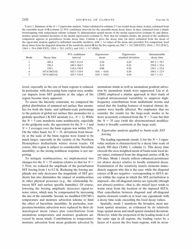
The leading eigenmode (mode 1) for the N � 5 eigen-value analysis is characterized by a decay time scale ofnearly 500 days (Table 1, column 1). This decay timeexceeds the area-weighted mean of basin-scale local de-cay times, estimated from the diagonal entries of G, by270 days. Mode 1 clearly reflects enhanced persistence(or slower decay) relative to locally estimated decay.Examination of the sensitivity matrix elements imme-diately suggests why this is the case: while the diagonalentries of G are negative—corresponding to SSTA de-cay within the region in which the SST perturbation isimposed—the off-diagonal entries are typically (thoughnot always) positive—that is, the mixed layer tends towarm away from the location of the imposed SSTA.Flux cancellation between diagonal and off-diagonalmatrix elements results in at least one eigenmode witha decay time scale exceeding the local decay values.

Spatially, mode 1 manifests the broadest, most uni-form spatial structure, as evidenced by its relativelylarge spatial mean and small spatial standard deviation.However, while the projection of the leading mode is ofthe same sign in all regions, the loading varies by afactor of 4 across the five basis regions, with its stron-

TABLE 1. Summary of the N � 5 eigenvalue analysis. Values tabulated in columns 2–5 are modal decay times, in days, estimated fromthe ensemble mean of G (column 2); 95% confidence intervals for the ensemble-mean decay times, in days, estimated from a simplebootstrapping with replacement scheme (column 3); dimensionless spatial means of the modal eigenvectors (column 4); and dimen-sionless spatial standard deviation of the modal eigenvectors (column 5). Note that for complex modes, the period of the oscillatorycomponent appears in parentheses beside decay time. Column 6 gives the decay time (in days) estimated from the mean ofthe eigenvalue analysis applied to individual ensemble members, with � 1� values of the mean also provided. For comparison, localdecay times from the diagonal elements of the sensitivity matrix G for the five regions are 384.7 � 14.2 (SH EXT), 184.6 � 39.5 (PAC),156.6 � 29.4 (NH EXT), 128.0 � 20.1 (ATL), and 110.1 � 9.7 (IND).

Mode Decay time95% confidence

intervalEigenvector

meanEigenvector

standard deviationIntraensemble

decay time

1 495.4 478.7–513.9 0.36 0.29 507.2 � 79.72 256.3 248.3–264.3 0.25 0.42 259.8 � 33.63 128.1 118.4–136.9 0.06 0.50 139.1 � 23.84 107.0 (4625.8) 103.7–110.9 0.01 � 0.01i 0.50 109.1 � 12.95 107.0 (4625.8) 103.7–110.9 0.01 � 0.01i 0.50 101.7 � 9.3


gest projection in the SH EXT region, where the localdecay time is largest. The lengthy decay of the SH EXTregion may simply reflect its large overall area and lowland-to-ocean ratio: longer decay is expected based onthe size of the SSTA and the fact that the ocean surfacearea is large compared to the radiating area of the top-of-the-atmosphere. In any event, the spatial heteroge-neity of the slowest decay mode reflects variations inbasic-state climatology: the leading eigenmode con-volves the broad scales anticipated for the most slowlydecaying mode with localized regions of slow decay.

The remaining eigenmodes exhibit decay character-istics reflecting the local decay features. For instance,the second mode decay time (�260 days) lies betweenthe decay time of SH EXT and the remaining regions.The second eigenvector is of one sign in SH EXT and ofopposite sign elsewhere. (Mode 3 behaves similarly, butwith the projection of one sign in PAC and oppositesign elsewhere.) The decay times of modes 4 and 5 areseen to be complex conjugates, indicating oscillatorydecaying behavior rather than strict exponential decay.However, since the period of oscillation is much longerthan the decay time, the complex modes are stronglyoverdamped and thus behave essentially like exponen-tially decaying modes.

One consideration in the interpretation of the eigen-value analysis is the statistical significance of the eigen-modes (e.g., how robust are the modal decay timescales?). Quantitative insight into statistical significancewas obtained through a simple bootstrapping with re-placement scheme (Efron 1982). Following standardprocedure, 1000 bootstrap G matrices were generatedby averaging 40 individual G matrices drawn at randomfrom the available simulated data. Eigenvalues of thebootstrap matrices were then computed and sorted, anda two-sided 95% confidence interval for each modaldecay time was estimated from the 25th and 975th val-ues (Table 1, column 3).

Overall, the bootstrapping analysis underscores verystable eigenvalues at the basin scale. For each mode,the width of the confidence interval is less than 10% ofthe ensemble-mean decay time scale. The bootstrap-ping results appear to be broadly consistent with un-certainty estimates based on the eigenvalues estimatedfrom the 40 individual members (Table 1, column 6).The latter provides some sense of how reliable esti-mates of decay characteristics would be for a singlethree-month average. For example, for the leadingeigenmode, the intraensemble standard deviation is ap-proximately 80 days. With an ensemble of 40, onewould anticipate, assuming Gaussian-distributed, un-correlated variance, an uncertainty of (80/401/2) � 13

days, which falls within the 95% bootstrap confidenceinterval.

c. Eigenvalue analysis applied to subbasin scales

We now turn to the N � 35 eigenvalue analysis. Al-though our principal emphasis here is on tropical decaycharacteristics, the results discussed include the extra-tropics (the “global case”). It is necessary to view tropi-cal SSTA decay in a global context since tropical–extratropical transports will potentially influence tropi-cal decay characteristics. However, because QTCM1 isnot optimized for extratropical dynamical accuracy,and the extratropics are incorporated into the analysisas spatially large basis regions, we will also considerwhat happens to the tropical decay characteristics whenthe extratropics are excluded from the analysis (the“tropics-only case”).

The spectrum of the real part of modal decay timesfor the global case, sorted from slowest to fastest, isillustrated in Fig. 2, with local decay time estimatesdisplayed for comparison. The leading mode, with�decay � 609 days, lies well above any of the local decayestimates. The nonleading modal decay times, by con-trast, fall below at least one of the local decay estimates.Also, as a consequence of the alteration to QTCM1’sadvection scheme, the leading mode decay time for N �35 is approximately 115 days longer than the leadingmode for N � 5.

Eigenvector loadings of the first three modes of theglobal case are displayed in Fig. 3. Like the leadingeigenmode of section 3b, the leading mode (Fig. 3a)

FIG. 2. Eigenmode decay times for the N � 35 basis regioneigenvalue analysis. Eigenmode decay times (days) are plotted assquares. The error bars shown are standard deviations of themodal decay times estimated from 1000 bootstrap samples. Forcomparison, local decay times, estimated from the diagonal en-tries of the flux sensitivity matrix G, are also shown (triangles).


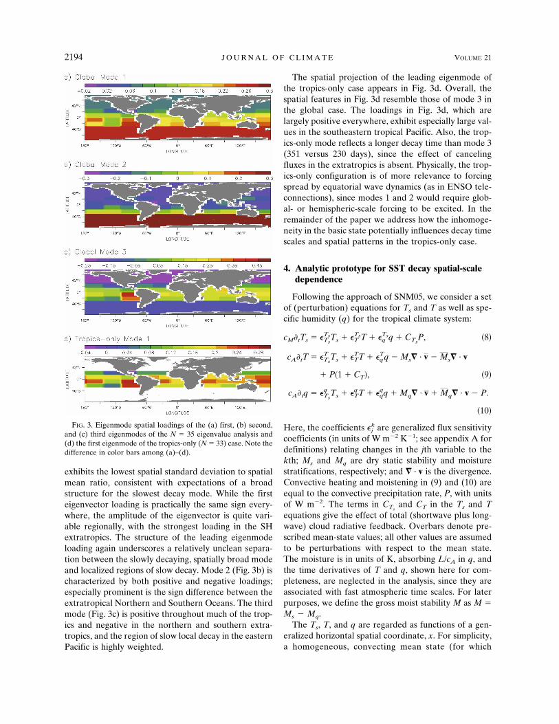
exhibits the lowest spatial standard deviation to spatialmean ratio, consistent with expectations of a broadstructure for the slowest decay mode. While the firsteigenvector loading is practically the same sign every-where, the amplitude of the eigenvector is quite vari-able regionally, with the strongest loading in the SHextratropics. The structure of the leading eigenmodeloading again underscores a relatively unclean separa-tion between the slowly decaying, spatially broad modeand localized regions of slow decay. Mode 2 (Fig. 3b) ischaracterized by both positive and negative loadings;especially prominent is the sign difference between theextratropical Northern and Southern Oceans. The thirdmode (Fig. 3c) is positive throughout much of the trop-ics and negative in the northern and southern extra-tropics, and the region of slow local decay in the easternPacific is highly weighted.

The spatial projection of the leading eigenmode ofthe tropics-only case appears in Fig. 3d. Overall, thespatial features in Fig. 3d resemble those of mode 3 inthe global case. The loadings in Fig. 3d, which arelargely positive everywhere, exhibit especially large val-ues in the southeastern tropical Pacific. Also, the trop-ics-only mode reflects a longer decay time than mode 3(351 versus 230 days), since the effect of cancelingfluxes in the extratropics is absent. Physically, the trop-ics-only configuration is of more relevance to forcingspread by equatorial wave dynamics (as in ENSO tele-connections), since modes 1 and 2 would require glob-al- or hemispheric-scale forcing to be excited. In theremainder of the paper we address how the inhomoge-neity in the basic state potentially influences decay timescales and spatial patterns in the tropics-only case.

4. Analytic prototype for SST decay spatial-scaledependence

Following the approach of SNM05, we consider a setof (perturbation) equations for Ts and T as well as spe-cific humidity (q) for the tropical climate system:

cM�tTs � �Ts

TsTs � �TTsT � �q

Tsq � CTsP, �8�

cA�tT � �Ts

T Ts � �TTT � �q

Tq � Ms� · v � Ms� · v

� P�1 � CT�, �9�

cA�tq � �Ts

q Ts � �TqT � �q

qq � Mq� · v � Mq� · v � P.

�10�

Here, the coefficients �kj are generalized flux sensitivity

coefficients (in units of W m�2 K�1; see appendix A fordefinitions) relating changes in the jth variable to thekth; Ms and Mq are dry static stability and moisturestratifications, respectively; and � · v is the divergence.Convective heating and moistening in (9) and (10) areequal to the convective precipitation rate, P, with unitsof W m�2. The terms in CTs

and CT in the Ts and Tequations give the effect of total (shortwave plus long-wave) cloud radiative feedback. Overbars denote pre-scribed mean-state values; all other values are assumedto be perturbations with respect to the mean state.The moisture is in units of K, absorbing L/cA in q, andthe time derivatives of T and q, shown here for com-pleteness, are neglected in the analysis, since they areassociated with fast atmospheric time scales. For laterpurposes, we define the gross moist stability M as M �Ms � Mq.

The Ts, T, and q are regarded as functions of a gen-eralized horizontal spatial coordinate, x. For simplicity,a homogeneous, convecting mean state (for which

FIG. 3. Eigenmode spatial loadings of the (a) first, (b) second,and (c) third eigenmodes of the N � 35 eigenvalue analysis and(d) the first eigenmode of the tropics-only (N � 33) case. Note thedifference in color bars among (a)–(d).


Fig 3 live 4/C

� · v�0) is considered. The flux sensitivity coefficientsare assumed spatially invariant, including the windspeed dependences in turbulent fluxes, and horizontaladvection is ignored. In the Betts and Miller (1986)convective scheme, P � CA(q � qc)/�c, where qc is theconvective reference humidity (treated here as a linearfunction of T, qc � �T, with � � 0.81) and �c is theconvective adjustment time scale. In what follows, thestrict QE limit (Neelin and Zeng 2000) of vanishinglysmall �c is invoked. Strict QE implies q → �T � �cP/CA,where P � �P

TsTs � �P

TT, with �PTs

� (Mq�TTs

� Ms�qTs

)/

(M � CTMq) and �PT � [Mq(�T

T � ��Tq) � �Ms�

qq]/(M �

CTMq).In addition to Eqs. (8)–(10), we consider a diagnostic

momentum balance between the baroclinic pressure(temperature) gradient and (surface) friction:

r�xT � �uuu. �11�

Here, r is the gas constant for air (287 J kg�1 K�1) and�u

u is the net momentum damping. Assuming separableform solutions [i.e., Ts(x, t) � ��T̃se

ikx/Ree�t], we obtaina dispersion relationship of the form

� � cM�1��Ts

Ts � CTs�Ts

P ��T

Ts � ��qTs � CTs

�TP��Ts

T � �Ts

q � CT�Ts

P �

�TT � ��q

T � �qq� � CT�T

P�1 � k2k02�� , �12�

where Re is the radius of the earth,

k0 � Re�1��T

T � ��qT � �q

q� � CT�TP�u

u

rM,

and L0 � Rek�10 defines a characteristic length scale

over which T anomalies behave coherently. The inverseof (12) is a generalized extension of (5).

Decay spectra for k0 � 0, 1, 2, and 3 with and withoutcloud radiative feedback effects are illustrated in Fig. 4.For the active cloud radiative feedback (solid lines),CT � 0.05 and CTs

��0.17. In the inviscid limit �uu → 0,

the scale defined by L0 becomes infinite (i.e., T fluc-tuations are uniform throughout the entire domain). Inthis weak temperature gradient (WTG) regime, SSTAdecay at all nonzero wavenumbers is fast compared tothe decay at wavenumber 0. For nonzero k0, there is asmooth transition between the slowest decay mode atk � 0 and the faster, effectively local decay values de-termined by �Ts

Tsfor k � k0. For parameter values rep-

resentative of the tropics in QTCM1 (M � 0.61 K, �uu �

�0.1 day�1, and �T*T � �33 W m�2 K�1 � �0.33

day�1), k0 � 1.5. Thus, we expect that only a smallnumber of modes should exhibit decay time scales dif-fering significantly from local decay values, in agree-ment with what is seen in Fig. 2.

Disabling the cloud radiative feedback (Fig. 4,dashed lines) increases the 1D prototype decay times,especially at nonzero wavenumber. The reason for thisincrease can be understood as follows: in the presenceof the feedback, a warm Ts anomaly increases precipi-tation, and hence the fraction of deep convectiveclouds, over the SSTA. The increased cloud cover de-creases the shortwave radiation incident on the surface(hence, CTs

� 0), which results in cooling, or fasterdecay than when the feedback is absent. The cloud ra-

diative feedback effect becomes less pronounced as theareal extent of the SSTA increases because the precipi-tation response per unit Ts is diminished since the termin �P

Tsopposes the term in �P

T.The diagnostic balance between baroclinic gradients

and frictional damping admits real (and decaying) so-lutions for �. However, other balances are plausible(e.g., baroclinic pressure gradients and momentum ad-vection). In general, this balance yields complex solu-tions for � (i.e., solutions that propagate as well as de-cay). Previously, Nilsson (2001) presented a frameworkfor understanding feedbacks between midlatitude sta-tionary atmospheric waves and SSTAs that is relevantto such decaying, propagating solutions. Such solutionsare likely to be of importance to a number of issuesbeyond the scope of this paper, including the develop-ment, maintenance, and timing of interbasin adjust-ment processes in the tropics.

5. Analytic prototype for differences betweenconvecting and nonconvecting regimes

The prototype developed in this section offers insightinto the separation between the fast local decay timesof tropical convecting regions and the slow local decayof nonconvecting regions. The prototype also shedslight on the interpretation of the eigenvalue analysis(section 3), specifically for understanding the blendingthat occurs between the broad-scale, slow decay modesand the slow, local decay times characteristic of tropicalnonconvecting regimes.

a. The N-box WTG model

Consider discretization of Eqs. (8)–(10) (again as-suming WTG) over a domain consisting of N boxes


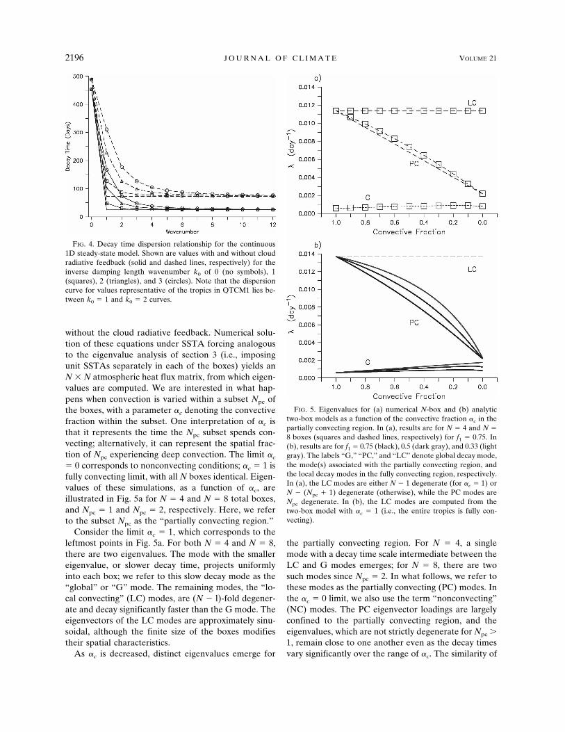
without the cloud radiative feedback. Numerical solu-tion of these equations under SSTA forcing analogousto the eigenvalue analysis of section 3 (i.e., imposingunit SSTAs separately in each of the boxes) yields anN N atmospheric heat flux matrix, from which eigen-values are computed. We are interested in what hap-pens when convection is varied within a subset Npc ofthe boxes, with a parameter �c denoting the convectivefraction within the subset. One interpretation of �c isthat it represents the time the Npc subset spends con-vecting; alternatively, it can represent the spatial frac-tion of Npc experiencing deep convection. The limit �c

� 0 corresponds to nonconvecting conditions; �c � 1 isfully convecting limit, with all N boxes identical. Eigen-values of these simulations, as a function of �c, areillustrated in Fig. 5a for N � 4 and N � 8 total boxes,and Npc � 1 and Npc � 2, respectively. Here, we referto the subset Npc as the “partially convecting region.”

Consider the limit �c � 1, which corresponds to theleftmost points in Fig. 5a. For both N � 4 and N � 8,there are two eigenvalues. The mode with the smallereigenvalue, or slower decay time, projects uniformlyinto each box; we refer to this slow decay mode as the“global” or “G” mode. The remaining modes, the “lo-cal convecting” (LC) modes, are (N � l)-fold degener-ate and decay significantly faster than the G mode. Theeigenvectors of the LC modes are approximately sinu-soidal, although the finite size of the boxes modifiestheir spatial characteristics.

As �c is decreased, distinct eigenvalues emerge for

the partially convecting region. For N � 4, a singlemode with a decay time scale intermediate between theLC and G modes emerges; for N � 8, there are twosuch modes since Npc � 2. In what follows, we refer tothese modes as the partially convecting (PC) modes. Inthe �c � 0 limit, we also use the term “nonconvecting”(NC) modes. The PC eigenvector loadings are largelyconfined to the partially convecting region, and theeigenvalues, which are not strictly degenerate for Npc �1, remain close to one another even as the decay timesvary significantly over the range of �c. The similarity of

FIG. 4. Decay time dispersion relationship for the continuous1D steady-state model. Shown are values with and without cloudradiative feedback (solid and dashed lines, respectively) for theinverse damping length wavenumber k0 of 0 (no symbols), 1(squares), 2 (triangles), and 3 (circles). Note that the dispersioncurve for values representative of the tropics in QTCM1 lies be-tween k0 � 1 and k0 � 2 curves.

FIG. 5. Eigenvalues for (a) numerical N-box and (b) analytictwo-box models as a function of the convective fraction �c in thepartially convecting region. In (a), results are for N � 4 and N �8 boxes (squares and dashed lines, respectively) for f1 � 0.75. In(b), results are for f1 � 0.75 (black), 0.5 (dark gray), and 0.33 (lightgray). The labels “G,” “PC,” and “LC” denote global decay mode,the mode(s) associated with the partially convecting region, andthe local decay modes in the fully convecting region, respectively.In (a), the LC modes are either N � 1 degenerate (for �c � 1) orN � (Npc � 1) degenerate (otherwise), while the PC modes areNpc degenerate. In (b), the LC modes are computed from thetwo-box model with �c � 1 (i.e., the entire tropics is fully con-vecting).


PC modal decay rates for small �c means that the par-tially convecting-region decay times are relatively in-sensitive to the size of the SSTA within the partiallyconvecting region, a point to which we return below.

The LC eigenvalue changes little as �c is varied. TheG mode eigenvalue also varies only slightly with �c,partly because the partially convecting region is a rela-tively small portion of the total domain but also forreasons elaborated below. When �c is small, the PCdecay times become comparable to the G mode decaytime. As a result, the eigenvectors of the G and PCmodes are altered in such a way that they become lessdistinct (i.e., the spatial properties of eigenvectors aremixed). In general, as �c decreases, the G mode eigen-vector loading in the partially convecting region is di-minished, and may even change sign. The PC mode, onthe other hand, tends to have opposite loadings in thepartially and fully convecting regions, with the loadingin the latter region decreasing as �c decreases.

b. A two-box model for the G and PC modes

The case for which the PC and G decay times aremuch slower than the LC decay time scales is relevantto the passively coupled tropical ocean–atmospheresystem. We exploit the separation of LC eigenvalues toreplace the arbitrary N-box model by a simple N � 2system. Box 1, with an area size fraction f1, is fullyconvecting, while box 2, with an area size fraction f2 �1 � f1, has specified convective fraction �c as in theN-box case. As with the prototype of section 4, strictQE and constant gross moist stability M are applied in

box 1 and the convecting portion of box 2. SSTAs im-posed in box 2 are assumed not to alter �c.

Although this model can be treated as a literal two-box model, its true utility lies in its capacity to approxi-mate the N-box model closely in certain parameterranges, eliminating redundant degenerate solutions.Furthermore, its straightforward analytic solution elu-cidates the behavior of the G and PC modes. Specifi-cally,

• The two-box solutions approximate the G and PCmodes over a large range of parameters (i.e., f1

greater than roughly 0.3, and small to modest �c). Inthe N-box case, the set of convecting-region boxes ischaracterized by identical eigenvector loadings forthe G and PC modes and may thus be replaced bybox 1 in the two-box model. This gives an excellentapproximation to these two modes, as seen in Fig. 5b.The case f1 � 0.75 may be compared to the numericalcase in Fig. 5a, with the caveat that the differencesseen are the result of using nonzero �c in the latter.(Note that the degenerate LC modes in Fig. 5b areobtained in a separate calculation; see the third bullet.)

• Analysis of the PC region time scale in the noncon-vecting (�c � 0) limit provides insight into why thepartially convecting region exhibits slow decay.

• Other limits of the two-box model are useful forother purposes (e.g., for f1 small and �c � 1, thetwo-box model yields the G and LC modes).

Analytic expressions for steady-state T, q, and � · vin the two-box framework are outlined in appendix B.Here we note that the 2 2 surface flux sensitivitymatrix to unit SSTAs is

G ��Ts

Ts � ��TTs � ��q

Ts�T�1, 0� �TTsT�1, 0� � �q

Tsq2�1, 0�

��TTs � ��q

Ts�T�0, 1� �Ts

Ts � �TTsT�0, 1� � �q

Tsq2�0, 1��, �13�

where T(1, 0) and T(0, 1) are tropospheric temperatureperturbation associated with unit SSTAs in boxes 1 and2, respectively, and q2(1, 0) and q2(0, 1) are box 2 mois-ture values for the same cases. The eigenvalues of (13)are simply �� 1⁄2(G11 � G22) � 1⁄2D1/2, where the dis-criminant D is given by D � (G11 � G22)2 � 4G12G21.

Some insight into the behavior of the eigenvalues canbe obtained by examining the behavior of the diagonaland off-diagonal matrix elements of G (Fig. 6). Con-sider parameters values for which the squared differ-ence between diagonal elements (Fig. 6a) is large com-pared to the product of the off-diagonal terms. Then,the eigenvalues are approximately given by G11 andG22. The behavior of G11 is easily understood. In

the limit of vanishing f1, T(1, 0) is identically zero, soG11 � �Ts

Ts. As �c increases, T(1, 0) increases (linearly),

and since �TsT and �Ts

q are of opposite sign to �TsTs

, themagnitude of G11 decreases. Thus, the two limits f1 � 0and f1 � 1 correspond to the fast LC and slow G modaldecay times, respectively.

As suggested by Fig. 6b, the off-diagonal terms G21

and G12 are generally small for the parameter valuesassumed here, especially G21, which represents the ef-fect of partially convecting-region SSTA on the fullyconvecting region. The smallness of the off-diagonalterms explains why the eigenvector loadings of the Gand PC modes are small in the partially and fully con-vecting regions, respectively. As Fig. 6a further indi-


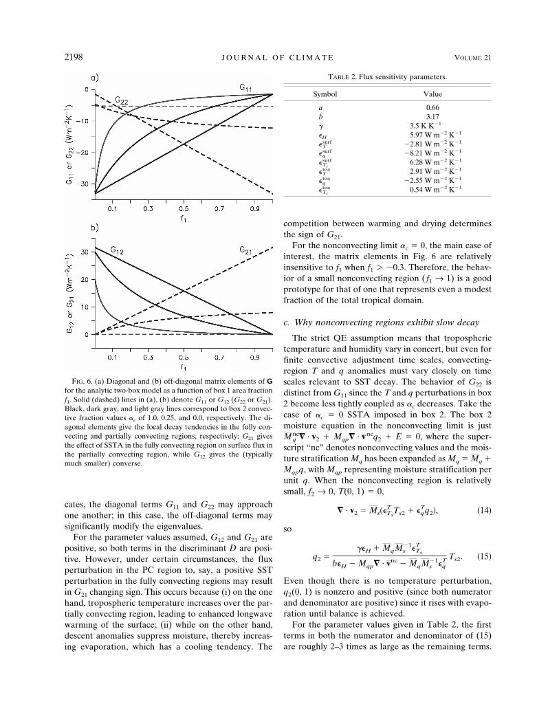
cates, the diagonal terms G11 and G22 may approachone another; in this case, the off-diagonal terms maysignificantly modify the eigenvalues.

For the parameter values assumed, G12 and G21 arepositive, so both terms in the discriminant D are posi-tive. However, under certain circumstances, the fluxperturbation in the PC region to, say, a positive SSTperturbation in the fully convecting regions may resultin G21 changing sign. This occurs because (i) on the onehand, tropospheric temperature increases over the par-tially convecting region, leading to enhanced longwavewarming of the surface; (ii) while on the other hand,descent anomalies suppress moisture, thereby increas-ing evaporation, which has a cooling tendency. The

competition between warming and drying determinesthe sign of G21.

For the nonconvecting limit �c � 0, the main case ofinterest, the matrix elements in Fig. 6 are relativelyinsensitive to f1 when f1 � �0.3. Therefore, the behav-ior of a small nonconvecting region ( f1 → 1) is a goodprototype for that of one that represents even a modestfraction of the total tropical domain.

c. Why nonconvecting regions exhibit slow decay

The strict QE assumption means that tropospherictemperature and humidity vary in concert, but even forfinite convective adjustment time scales, convecting-region T and q anomalies must vary closely on timescales relevant to SST decay. The behavior of G22 isdistinct from G11 since the T and q perturbations in box2 become less tightly coupled as �c decreases. Take thecase of �c � 0 SSTA imposed in box 2. The box 2moisture equation in the nonconvecting limit is justMnc

q � · v2 � Mqp� · vncq2 � E � 0, where the super-script “nc” denotes nonconvecting values and the mois-ture stratification Mq has been expanded as Mq � Mq �Mqpq, with Mqp representing moisture stratification perunit q. When the nonconvecting region is relativelysmall, f2 → 0, T(0, 1) � 0,

� · v2 � Ms��Ts

T Ts2 � �qTq2�, �14�

so

q2 ��H � MqMs

�1�Ts

T

b�H � Mqp� · vnc � MqMs�1�q

T Ts2. �15�

Even though there is no temperature perturbation,q2(0, 1) is nonzero and positive (since both numeratorand denominator are positive) since it rises with evapo-ration until balance is achieved.

For the parameter values given in Table 2, the firstterms in both the numerator and denominator of (15)are roughly 2–3 times as large as the remaining terms.

FIG. 6. (a) Diagonal and (b) off-diagonal matrix elements of Gfor the analytic two-box model as a function of box 1 area fractionf1. Solid (dashed) lines in (a), (b) denote G11 or G12 (G22 or G21).Black, dark gray, and light gray lines correspond to box 2 convec-tive fraction values �c of 1.0, 0.25, and 0.0, respectively. The di-agonal elements give the local decay tendencies in the fully con-vecting and partially convecting regions, respectively; G21 givesthe effect of SSTA in the fully convecting region on surface flux inthe partially convecting region, while G12 gives the (typicallymuch smaller) converse.

TABLE 2. Flux sensitivity parameters.

Symbol Value

a 0.66b 3.17� 3.5 K K�1

�H 5.97 W m�2 K�1

�surfT �2.81 W m�2 K�1

�surfq �8.21 W m�2 K�1

�surfTs

6.28 W m�2 K�1

�toaT 2.91 W m�2 K�1

�toaq �2.55 W m�2 K�1

�toaTs

0.54 W m�2 K�1


Expanding the denominator to first order in termssmall compared to b�H, q2 becomes

q2 � �b�1 � �Mqp� · vnc��b�H� � �Mq�Ts

T Ms��H�

� �Mq�qTMs��b�H�. �16�

The latent heating, sensible heating, and net surfaceradiative components of the total surface heat flux forthe nonconvecting region (i.e., G22) are

E � ��Mqp b�� · vnc � �Mq Ms��Ts

surf � �Ts

toa � �H�

� �b��Mq Ms��qsurf � �q

toa�Ts2, �17�

H � �HTs2, �18�

Rs � �Ts

surf � �qsurf�b�Ts2. �19�

The evaporation comprises contributions from (slow)mean subsidence [the first term on the rhs of (17)] aswell as feedback terms associated with changes to cir-culation. The contribution of the mean subsidenceterm, which is the largest single component of the netsurface flux, implies E � moisture divergence. The re-maining terms are associated with atmospheric absorp-tion of anomalous fluxes from the surface, which lead toanomalous ascent opposing the climatological descent.The resulting decrease in evaporation tends to partiallycompensate for upward surface fluxes, for example,longwave radiation and sensible heat flux, Eqs. (18) and(19), that act to cool SST. As an example, consider theeffect of the term associated with upward longwave ra-diative cooling of the surface associated with the directeffect of anomalously warm SSTA [the first term on therhs of (19)]. Writing the portion of emitted longwaveradiation absorbed by the atmosphere as � � (�s

Ts�

�tTs

)/�sTs

, the net cooling when including the feedbackeffect in evaporation reduces the direct longwave cool-ing by a factor of approximately (1 � MqM�1

s �). SinceMq is a large fraction of Ms and a large fraction oflongwave is absorbed, this amounts to a substantial re-duction. Similar arguments apply to the longwave fluxassociated with changes to moisture as well as the sen-sible heating.

For a small nonconvecting region, the rate of evapo-rative cooling is limited by the slow moisture diver-gence; other forms of surface cooling are reduced byfeedbacks via the circulation onto evaporation. This re-sults in a much slower decay than for a small convectingregion. An alternative perspective on the slowness ofnonconvecting-region decay was developed by Chiangand Sobel (2002). Specifically, in the absence of deepconvection, the communication between the free tro-pospheric temperature and the surface is limited, sincethe time scale for vertical advective transport is much

slower than the time scale for vertical convective trans-port. Because q and T are effectively decoupled withinnonconvecting regions, the former can buffer surfacetemperature from the free tropospheric temperature,which restricts the capacity for SSTA decay.

The behavior of G22 further suggests that noncon-vecting-region decay times should barely change as thesize of the nonconvecting region is varied (for a regionwith small �c). This is because there is no convectivefeedback on the warming by surface fluxes, so T re-mains small, and the balances remain similar to theanalysis for small f2.

d. Merger of the G and NC modes

Previously, we noted the role of horizontal transportsin setting decay time scales, particularly for the mostslowly decaying modes. For the results displayed in Fig.5, the damping coefficients �tr

T and �trq , representing

transport to the extratropics, are set to zero, resulting inrather long (�1000 day) decay times for the G mode.However, small changes to these damping coefficientscan have a strong impact on the eigenvalues: in Fig. 7a,the two damping coefficients (assumed equal for sim-plicity) were varied over a realistic range of values forf1 � 0.6 for �c � 0. By increasing, say, the T damping,the tropospheric temperature warming is lowered rela-tive to the no-damping situation; this results in a de-crease in G11 (G22 also decreases, but the change is lesspronounced). Thus, the nonconvecting-region modeand global decay mode eigenvalues increase—and infact converge—as the damping increases.

For zero damping and f1 � 0.6, G12 and G21 are bothsmall, so the off-diagonal terms have little impact onthe eigenvalues. However, the convergence of diagonalmatrix elements as damping increases means that theoff-diagonal terms may become more significant. Infact, as the damping increases beyond �tr

T � 0.3, the signof G21 changes for the reason discussed in section 5b.The discriminant changes sign when (G11 � G22)2 be-comes less than 4G12G21. Thus, a complex conjugatepair replaces the two real eigenvalues for damping val-ues greater than �tr

T � 1.85 W m�2 K�1.This case provides a simple illustration of the blend-

ing of properties that may occur between eigenmodes.This can occur even if the eigenvalues do not becomeequal, as in the case shown, but simply become suffi-ciently close to one another. In particular, the proper-ties of the G mode—which for physically realistic cli-matologies is the most slowly decaying mode character-ized by the broadest spatial scale—become mixed withthe properties of slowly decaying PC modes. This be-havior can account for some of the spatial inhomoge-neity seen in the eigenvalue analysis of the full QTCM1


simulations (section 3). The regions of slowest localdecay appear with high loadings in the slow globalmode of the tropical case because of this blending ef-fect, since the time scales are not well separated. Theslow nonconvecting regions can appear with either signin the G mode for either of two reasons. One is if theeffect of convecting-region SSTA actually creates acooling in the nonconvecting region, as noted above.The other, as seen for instance in Fig. 3, is simply thatif there is more than one slow decay region, they willtend to occur with opposite sign in the leading eigen-modes.

6. Summary and conclusions

The spatial inhomogeneity of SSTA autocorrelationtimes in atmospheric models (CCM3 and QTCM1),when coupled to an ocean mixed layer, motivates asystematic study of the modes of the passively coupledsystem. When inhomogeneity is ignored, the physicsunderlying the local and global decay time scales isstraightforward. For small-scale SST anomalies, decaytimes are typically rapid, with e-folding times of theorder 50–100 days for a 50-m mixed layer. Because theatmospheric response to a localized heating anomaly isspread by transport over large distances, mixed layerheat content is rapidly extracted from sufficiently local-ized anomalies. As the areal extent of the SSTA in-creases, the decay rate becomes progressively limitedby relatively slow top-of-the-atmosphere radiativetransfer. Consequently, for a global SSTA, for whichthe size of the anomaly is comparable to the total ra-diating area of the atmosphere, the decay time for a50-m mixed layer exceeds 500 days.

Under more realistic conditions, the transition be-tween the fast local and slow global scales is nontrivial.Within the tropics, efficient horizontal wave dynamicscommunicates the heating from local sources over theextent of the equatorial waveguide, �20°S–20°N.Eigenvalue analysis applied to idealized simulations ofQTCM1 indicates that local decay is a reasonable ap-proximation for spatial scales smaller than either thetropical Atlantic or Indian Ocean basins. Extratropicalwave dynamics also affects SST decay characteristics,although in a more complicated way (e.g., nonlineari-ties associated with midlatitude wave dynamics imparta nontrivial structure to the passive decay characteris-tics).

A major focus of this study concerned the impact ofbasic-state climate on tropical decay characteristics. Inthis vein, we noted the distinct separation of local tropi-cal SST decay time scales for mean convecting and non-convecting regions, with the latter exhibiting decaytime scales several times longer than the former. Thereasons for such separation were highlighted in section5: for nonconvecting regions, the dominant balance isbetween slow moisture divergence via the subsidingmean flow and evaporation. In the absence of a con-vective moisture sink, sizable tropospheric humidityanomalies develop in response to SSTAs imposedwithin the nonconvecting region: these anomalies limitthe rate of evaporation to a value given by the slowmoisture divergence, in turn implying a slow rate ofSST decay. Longwave radiation emitted by the surfaceis substantially absorbed in the atmosphere, which

FIG. 7. Eigenmode properties as a function of horizontal trans-port/damping coefficients �tr

T and �trq . The case shown corresponds

to f1 � 0.6 and �c � 0, that is, the partially convecting region isnonconvecting, with �tr

T � �trq . (a) Eigenvalues (day�1) for the PC

mode (solid line) and G mode (dashed line). Note that for valuesof coefficients exceeding 1.84 W m�2 K�1, the eigenvalues com-prise a complex conjugate pair. (b) Eigenvalue loadings for thetwo modes in the fully convecting region (top two curves) and thepartially convecting region (bottom two curves). (c) Ratios ofeigenvector standard deviations to eigenvector means for the twomodes.


slows moisture divergence, and therefore has a limitedimpact on SSTA decay characteristics.

The slow decay of nonconvecting regions has signif-icant implications for the spatial structure of passiveocean–atmosphere decay modes, especially the slowlydecaying global mode. While the global decay modemight be expected to exhibit a broad, uniform spatialstructure, this assumption does not hold in the presenceof basic-state inhomogeneities: although eigenvalueanalysis indicates a relatively broad structure for themost slowly decaying mode, it is spatially heteroge-neous. In particular, the features of the global decaymode are blended or mixed with the localized, slowdecay characteristics of nonconvecting areas. Preciselyhow this blending affects the eigenmodes depends sen-sitively on a number of factors (e.g., the closeness ofdecay mode time scales), and the loading of slowestdecay mode in the nonconvecting region can have rela-tively small or large amplitude or even change sign. Ifthe nonconvecting and global mode time scales ap-proach each other, a merger may even occur. In theeigenvalue analysis of QTCM1, the most visible signa-ture is large eigenvector loadings of the slow, leadingeigenmodes in localized slowly decaying regions.

Although we have framed our analysis largely interms of the decay of SSTAs, the results also apply topassive mixed layer equilibration to a prescribed cli-mate forcing (e.g., the remote tropical climate responseto El Niño or the transient upper ocean adjustment toatmospheric radiative anomalies associated with green-house gases or aerosols). For instance, SNM05 arguedthat tropical tropospheric warming to El Niño can beviewed in two stages: a fast stage, associated with en-ergy loss to the unadjusted remote mixed layer, and aslower stage—essentially the global tropical decay timescale—limited by top-of-the-atmosphere radiativelosses and tropical–extratropical energy export.

The results of our study add a further layer of com-plexity to the picture of the tropospheric temperatureadjustment to El Niño, specifically with respect to theimpacts of basic-state inhomogeneities. Consider, forexample, the tropical Atlantic. Because of the NorthernHemisphere bias of the intertropical convergence zone,the north tropical Atlantic is, on average, more stronglyconvecting than the south tropical Atlantic. Thus, weanticipate modifications to the rate of troposphericwarming from the local convective and nonconvectiveregion decay modes operating to the north and south ofthe equator, respectively. We thus conjecture that theinhomogeneous passive decay modes examined heremay be useful ingredients in understanding the ob-served tendency for an equatorially asymmetric tropicalAtlantic surface temperature response to El Niño, with

regions north of the equator warming more, and withdifferent timing, than those to the south (Enfield andMayer 1997; Elliott et al. 2001; Chiang and Sobel 2002).Equally intriguing, and warranting further study, is howthe slow decay region in the nonconvecting southeast-ern tropical Pacific, encountered here with only passivecoupling, interacts with ocean dynamics in the ENSOsource region.

Acknowledgments. We thank J. C. H. Chiang for pro-viding the CCM3 mixed layer simulation. We alsothank J. T. Farrar, C. Holloway, A. H. Sobel, J. Nilsson,and two anonymous reviewers for valuable discussionand comments on the manuscript. This work was sup-ported in part by NOAA Grants NA04OAR4310013and NA05OAR4310007 and NSF Grant ATM-0645200.BRL further acknowledges partial support by J. C. H.Chiang and NOAA Grant NA03OAR4310066.

APPENDIX A

Flux Sensitivity Coefficients

The flux sensitivity coefficients are defined analo-gously to SNM05. The values assumed are representa-tive of clear-sky conditions. These coefficients are

�Ts

Ts � �Ts

surf � �H � �H, �A1�

�qTs � b�H � �q

surf, �A2�

�TTs � a�H � �T

surf, �A3�

�Ts

T � �H � �Tsurf

s � �Ts

toa, �A4�

�Ts

q � �H, �A5�

�TT � �T

surf � �Ttoa � a�H � �T

tr, �A6�

�qT � �q

surf � �qtoa, �A7�

�Tq � 0, and �A8�

�qq � �b�H � �q

tr. �A9�

In the above expressions, a and b relate the QTCM1vertical structure functions of temperature and mois-ture to their surface values, respectively. The coeffi-cient �, defined as �qs/�Ts, where qs is saturation spe-cific humidity at the surface, follows from the lineariza-tion of evaporation; it is evaluated with respect to areference temperature, taken here to be 302 K. Valuesof the flux sensitivity parameters are summarized inTable 2. The temperature and moisture transport coef-ficients, �tr

T and �trq , are treated as adjustable param-

eters.


APPENDIX B

Analytic Solutions to the Two-Box Model

Using the labeling conventions of section 6, the tem-perature perturbation to an arbitrary distribution ofSSTs Ts1 and Ts2 is

T�Ts1, Ts2� � T*�Mc�1� f1 � f2�c��TT � ��q

T � �qq�

� �1 � �c�f2�TTC1�

�1, �B1�

where

T* � �Mc�1��Ts

T � �Ts

q �� f1Ts1 � f1�cTs2�

� �1 � �c�f2C1C2Ts2 and

C1 � �Msnc �

�qTMq

nc

Mqp� · vnc � �qq��1

and

C2 � �Ts

T ��q

T�Ts

q

Mqp� · vnc � �qq .

For box 1, the humidity perturbation is, by the strictQE assumption, just q1(Ts1, Ts2) � �T(Ts1, Ts2). Forbox 2, on the other hand,

q2�Ts1, Ts2� � �c�T � �1 � �c��Ts

q Ts2 � Mqnc� · v2�

�Mqp� · vnc � �qq��1, �B2�

where � · v2(Ts1, Ts2) � C1[C2Ts2 � �TTT( f1, �c)]. Plots

of the temperature and humidity anomalies in responseto separate 1-K SST perturbations in each box are il-lustrated in Fig. B1.

REFERENCES

Alexander, M. A., I. Bladé, M. Newman, J. R. Lanzante, N.-C.Lau, and J. D. Scott, 2002: The atmospheric bridge: The in-fluence of ENSO teleconnections on air–sea interaction overthe global oceans. J. Climate, 15, 2205–2231.

Barsugli, J. J., and D. S. Battisti, 1998: The basic effects of atmo-sphere–ocean thermal coupling on midlatitude variability. J.Atmos. Sci., 55, 477–493.

Battisti, D. S., 1988: Dynamics and thermodynamics of a warmingevent in a coupled tropical atmosphere–ocean model. J. At-mos. Sci., 45, 2889–2919.

Betts, A. K., and M. J. Miller, 1986: A new convective adjustmentscheme. Part II: Single column tests using GATE wave,BOMEX, ATEX and Arctic air-mass data sets. Quart. J. Roy.Meteor. Soc., 112, 693–709.

Bhatt, U. S., M. A. Alexander, D. S. Battisti, D. D. Houghton,and L. M. Keller, 1998: Atmosphere–ocean interaction in theNorth Atlantic: Near-surface climate variability. J. Climate,11, 1615–1632.

Bretherton, F. P., 1982: Ocean climate modeling. Prog. Oceanogr.,11, 93–129.

Cane, M. A., and S. E. Zebiak, 1986: On the mechanism of the ElNiño-Southern Oscillation cycle. Study Week on PersistentMeteo-Oceanographic Anomalies and Teleconnections, C.Chagas and G. Puppi, Eds., Pontificia Academia Scientiarum,6–96.

Chang, P., L. Ji, H. Li, C. Penland, and L. Matrosova, 1998: Pre-diction of tropical Atlantic sea surface temperature. Geo-phys. Res. Lett., 25, 1193–1196.

Chiang, J. C. H., and A. H. Sobel, 2002: Tropical tropospherictemperature variations caused by ENSO and their influenceon the remote tropical climate. J. Climate, 15, 2616–2631.

——, and B. R. Lintner, 2005: Mechanisms of remote tropicalsurface warming during El Niño. J. Climate, 18, 4130–4149.

Chou, C., and J. D. Neelin, 2004: Mechanisms of global warmingimpacts on regional tropical precipitation. J. Climate, 17,2688–2701.

——, ——, J.-Y. Tu, and C.-T. Chen, 2006: Regional tropical pre-cipitation change mechanisms in ECHAM4/OPYC3 underglobal warming. J. Climate, 19, 4207–4223.

FIG. B1. (a) Tropospheric temperature and (b) box 2 humidityanomalies for the analytic two-box model as a function of box 1area fraction f1. Solid lines are for an imposed 1-K SST perturba-tion in box 1 (the fully convecting region), and dashed lines are foran imposed 1-K SST perturbation in box 2 (the partially convect-ing region). Black, dark gray, and light gray lines correspond tobox 2 convective fraction values �c of 1.0, 0.25, and 0.0, respec-tively.


Deser, C., M. A. Alexander, and M. S. Timlin, 2003: Understand-ing the persistence of sea surface temperature anomalies inmidlatitudes. J. Climate, 16, 57–72.

Efron, B., 1982: The Jackknife, the Bootstrap, and Other Resam-pling Plans. Society for Industrial and Applied Mathematics,92 pp.

Elliott, J. R., S. P. Jewson, and R. T. Sutton, 2001: The impact ofthe 1997/98 El Niño event on the Atlantic Ocean. J. Climate,14, 1069–1077.

Enfield, D. B., and D. A. Mayer, 1997: Tropical Atlantic sea sur-face temperature variability and its relation to El Niño-Southern Oscillation. J. Geophys. Res., 102, 929–945.

Frankignoul, C., 1985: Sea surface temperature anomalies, plan-etary waves, and air-sea feedback in the middle latitudes.Rev. Geophys., 23, 357–390.

——, and K. Hasselmann, 1977: Stochastic climate models. II:Application to sea-surface temperature anomalies and ther-mocline variability. Tellus, 29, 289–305.

Gallego, B., and P. Cessi, 2001: Decadal variability of two oceansand an atmosphere. J. Climate, 14, 2815–2832.

Giannini, A., J. C. H. Chiang, M. A. Cane, Y. Kushnir, and R.Seager, 2001: The ENSO teleconnection to the tropical At-lantic Ocean: Contributions of the remote and local SSTs torainfall variability in the tropical Americas. J. Climate, 14,4530–4544.

Grabowski, W. W., 2006: Impact of explicit atmosphere–oceancoupling on MJO-like coherent structures in idealized aqua-planet simulations. J. Atmos. Sci., 63, 2289–2306.

Hansen, J., and Coauthors, 1997: Forcings and chaos in interan-nual to decadal climate change. J. Geophys. Res., 102, 25 679–25 720.

Hasselmann, K., 1976: Stochastic climate models. Part I: Theory.Tellus, 28, 473–485.

Kara, A. B., P. A. Rochford, and H. E. Hurlburt, 2003: Mixedlayer depth variability over the global ocean. J. Geophys.Res., 108, 3079, doi:10.1029/2000JC000736.

Kiehl, J. T., J. J. Hack, G. B. Bonan, B. A. Boville, D. L. William-son, and P. J. Rasch, 1998: The National Center for Atmo-spheric Research Community Climate Model: CCM3. J. Cli-mate, 11, 1131–1149.

Klein, S. A., B. J. Soden, and N.-C. Lau, 1999: Remote sea surfacetemperature variations during ENSO: Evidence for a tropicalatmospheric bridge. J. Climate, 12, 917–932.

Kushnir, Y., W. A. Robinson, I. Bladé, N. M. J. Hall, S. Peng, andR. Sutton, 2002: Atmospheric GCM response to extratropicalSST anomalies: Synthesis and evaluation. J. Climate, 15,2233–2256.

Lin, J. W.-B., J. D. Neelin, and N. Zeng, 2000: Maintenance oftropical intraseasonal variability: Impact of evaporation–wind feedback and midlatitude storms. J. Atmos. Sci., 57,2793–2823.

Maloney, E. D., and A. H. Sobel, 2004: Surface fluxes and oceancoupling in the tropical intraseasonal oscillation. J. Climate,17, 4368–4386.

Marotzke, J., and D. W. Pierce, 1997: On spatial scales and life-times of SST anomalies beneath a diffusive atmosphere. J.Phys. Oceanogr., 27, 133–139.

Marshall, J., and Coauthors, 2001: North Atlantic climate vari-ability: Phenomena, impacts and mechanisms. Int. J. Clima-tol., 21, 1863–1898.

Münnich, M., M. Latif, S. Venzke, and E. Maier-Reimer, 1998:Decadal oscillations in a simple coupled model. J. Climate,11, 3309–3319.

Neelin, J. D., and W. Weng, 1999: Analytical prototypes forocean–atmosphere interaction at midlatitudes. Part I:Coupled feedbacks as a sea surface temperature dependentstochastic process. J. Climate, 12, 697–721.

——, and N. Zeng, 2000: A quasi-equilibrium tropical circulationmodel—Formulation. J. Atmos. Sci., 57, 1741–1766.

——, and H. Su, 2005: Moist teleconnection mechanisms for thetropical South American and Atlantic sector. J. Climate, 18,3928–3950.

——, D. S. Battisti, A. C. Hirst, F.-F. Jin, Y. Wakata, T. Yama-gata, and S. E. Zebiak, 1998: ENSO theory. J. Geophys. Res.,103, 14 261–14 290.

Nilsson, J., 2000: Propagation, diffusion, and decay of SST anoma-lies beneath an advective atmosphere. J. Phys. Oceanogr., 30,1505–1513.

——, 2001: Spatial reorganization of SST anomalies by stationaryatmospheric waves. Dyn. Atmos. Oceans, 34, 1–21.

Park, S., C. Deser, and M. A. Alexander, 2005: Estimation of thesurface heat flux response to sea surface temperature anoma-lies over the global oceans. J. Climate, 18, 4582–4599.

Philander, S. G. H., T. Yamagata, and R. C. Pacanowski, 1984:Unstable air–sea interactions in the tropics. J. Atmos. Sci., 41,604–613.

Saravanan, R., and P. Chang, 2000: Interaction between tropicalAtlantic variability and El Niño–Southern Oscillation. J. Cli-mate, 13, 2177–2194.

Schopf, P. S., 1985: Modeling tropical sea-surface temperature:Implication of various atmospheric responses. CoupledOcean-Atmosphere Models, J. C. J. Nihoul, Ed., Elsevier,727–734.

Sobel, A. H., and H. Gildor, 2003: A simple time-dependentmodel of SST hot spots. J. Climate, 16, 3978–3992.

Su, H., J. D. Neelin, and J. E. Meyerson, 2003: Sensitivity of tropi-cal tropospheric temperature to sea surface temperature forc-ing. J. Climate, 16, 1283–1301.

——, ——, and ——, 2005: Mechanisms for lagged atmosphericresponse to ENSO SST forcing. J. Climate, 18, 4195–4215.

Tang, B. H., and J. D. Neelin, 2004: ENSO influence on Atlantichurricanes via tropospheric warming. Geophys. Res. Lett., 31,L24204, doi:10.1029/2004GL021072.

Timlin, M. S., M. A. Alexander, and C. Deser, 2002: On the re-emergence of North Atlantic SST anomalies. J. Climate, 15,2707–2712.

Watanabe, M., and M. Kimoto, 2000: On the persistence of de-cadal SST anomalies in the North Atlantic. J. Climate, 13,3017–3028.

Wu, Z.-X., and R. E. Newell, 1998: Influence of sea surface tem-peratures on air temperatures in the tropics. Climate Dyn.,14, 275–290.

Zeng, N., J. D. Neelin, and C. Chou, 2000: A quasi-equilibriumtropical circulation model—Implementation and simulation.J. Atmos. Sci., 57, 1767–1796.

Zhang, C. D., M. Dong, S. Gualdi, H. H. Hendon, E. D. Maloney,A. Marshall, K. R. Sperber, and W. Q. Wang, 2006: Simula-tions of the Madden–Julian oscillation in four pairs ofcoupled and uncoupled global models. Climate Dyn., 27, 573–592.


time scales and spatial patterns of passive ocean

Documents