time optimal control of a right invariant system on a
TRANSCRIPT

TIME OPTIMAL CONTROL OF A RIGHT INVARIANT SYSTEMON A COMPACT LIE GROUP
JODY-LYNN STORM
Abstract. In this paper we will study the pulse sequences in NMR spec-
troscopy and quantum computing as a time control problem. Radio frequency
pulses are used to execute a unitary transfer of state. Sequences of pulses should
be as short as possible to minimize decoherence. We model the problem as a
controllable right invariant system on a compact Lie group. We investigate the
minimum time required to steer the system from an initial point to a specified
final point.
1. Introduction
Richard Feynman was one of the first individuals to recognize that there is anexponential slowdown when classical computers are used to simulate quantum sys-tems. He went on to suggest that the use of quantum computers to simulate quan-tum systems should be exponentially faster than their classical counterparts.
In 1994, Peter Shor devised an algorithm for quantum computers that could fac-tor integers exponentially faster than the best-known classical factoring algorithm.Shor’s algorithm means, that if quantum computers could be built, then crypto-graphic systems based on factoring, like those commonly used in banking, could bebroken. Expanding on Shor’s algorithm, in 1996, Lov Grover created a quantumalgorithm that could search databases faster than anything possible on classicalcomputers.
A technique that has been used to build elementary quantum computers is nu-clear magnetic resonance (NMR), a physical phenomenon based upon the quantummechanical magnetic properties of an atom’s nucleus. The elementary particles,neutrons and protons, composing an atomic nucleus have the intrinsic quantummechanical property of angular momentum, called spin. In NMR, unitary transfor-mations are used to manipulate an ensemble of nuclear spins. However, the sequenceof pulses that generate the desired unitary operator should be as short as possiblein order to minimize the effects of decoherence; a major obstacle faced in buildingquantum computers. Quantum systems want to wander from their computationalpath and entangle with the rest of the environment. Transferring quantum states
Date: October 28, 2008.
I would like to thank Dr. George Wilkens for his patience, knowledge and support.
1

2 JODY-LYNN STORM
as quickly as possible helps minimize the impact of decoherence, and thus motivatesthe minimum time problem.
In this paper we will study the design of pulse sequences in NMR spectroscopy(measurement of a quantity as function of either wavelength or frequency) as a timeoptimal control problem on a compact Lie group. In quantum computation, allowedoperations are unitary matrices, which are effectively rotations, so our primaryinterest will be in the unitary group U(n), although the discussion is general enoughto include other compact Lie groups such as SO(n). The question we will addressis the problem of time control. If we are given a controllable right invariant systemon a compact Lie group, what is the minimum time required to steer the systemfrom an initial point to a specified final point?
We will present a mathematical formulation for the problem of finding the short-est pulse sequences in NMR. We will also show that the problem of computing min-imum time to produce a unitary propagator can be reduced to finding the shortestlength paths on certain coset spaces.
Control Systems. The time evolution of a quantum system is described by thetime dependent Schroedinger equation
U(t) = −iH(t)U(t), U(0) = I,
where H (t) is the Hamiltonian and U (t) is the unitary displacement. We can writethe Hamiltonian as
H(t) = Hd +m∑i=1
vi(t)Hi,
where Hd is the part of the Hamiltonian internal to the system, called the drift,and
∑mi=1 vi(t)Hi(t) is the part of the Hamiltonian that can be externally changed,
which we call the control.We are interested in finding the minimum time required to transfer the system
U = −i[Hd +m∑i=1
viHi]U
from U(0) = I, to a final state UF .
2. Preliminaries
Definition. A smooth (or differentiable) manifold of dimension n is a second-countable, Hausdorff topological space M with a collection of pairs (Uα, φα), calledcharts, where Uα is an open subset of M and φα : Uα → Rn so that:
(a) Each φα is a homeomorphism of Uα onto an open subset Vα of Rn.(b)
⋃α Uα = M .

TIME OPTIMAL CONTROL 3
(c) For every α, β the transition functions φαβ = φβ φ−1α : φα(Uα ∩ Uβ) →
φβ(Uα∩Uβ) are smooth, in the sense of smooth functions between subsetsof Rn, i.e. φαβ is C∞. In this case the charts (Uα, φα) and (Uβ , φβ) arecalled compatible.
(d) The family (Uα, φα) is maximal relative to the conditions (b) and (c).
Such a family of sets and maps satisfying (b),(c), and (d) constitutes a differentiablestructure on M .
Example. The Euclidean space Rn is an n-dimensional manifold whose differentiablestructure consists of all charts that are compatible with the chart (U, φ) whereU = Rn and φ : U → Rn is the identity map.
Definition. Let p be a point of a manifold M . Let F(M) be the set of all smoothreal-valued functions on M . A tangent vector to M at p is a real-valued functionv : F(M)→ R that satisfies:
(1) v(af + bg) = av(f) + bv(g),(2) v(fg) = v(f)g(p) + f(p)v(g), for a, b ∈ R, f, g ∈ F(M).
For each p ∈M , let Tp(M) be the set of all tangent vectors to M at p. Then underthe operations
(v + w)(f) = v(f) + w(f),
(av)(f) = av(f),
the set Tp(M) is a real vector space, called the tangent space of M at p.
By a standard proposition in differential geometry, the dimension of Tp(M) equalsthat of M . The tangent bundle of M is the union, over all p in M , of the tangentspaces Tp(M). The tangent bundle is denoted by TM .
Definition. Let F : M → N be a function, where M and N are smooth manifolds.Then F is smooth (differentiable) if for every smooth, real valued function f ∈ F(N)the composite function f F ∈ F(M). Let p ∈ M . The derivative of F at p isthe function dFp : Tp(M) → TF (p)(N) such that for every vp ∈ Tp(M) and everyf ∈ F(N), dFp(vp)f = vp (f F ).
A vector field X on a manifold M is a function that assigns to each point p ∈Ma tangent vector Xp to M at p. Thus X : M → TM with Xp ∈ TpM . If X is avector field on M and f ∈ F(M), then Xf denotes the real-valued function on M
given byXf(p) = Xp(f), ∀p ∈M.
The vector field X is called smooth if the function Xf is smooth for all f ∈ F(M).
Definition. Let G be a smooth manifold. Then G is called a Lie Group if:
(a) G is a group

4 JODY-LYNN STORM
(b) The group operations G × G → G defined by (x, y) 7→ xy and G → G
defined by x 7→ x−1 are smooth (differentiable) functions.
Example. The set Rn is a Lie group under vector addition.
Definition. A Lie algebra g is a vector space over a field F with a binary operation[. , .] : g× g→ g called the Lie bracket, which satisfies the following axioms:
(a) Bilinearity
[aX + bY, Z] = a[X,Z] + b[Y, Z], [Z, aX + bY ] = a[Z,X] + b[Z, Y ]
for all scalars a, b ∈ F and all X,Y, Z ∈ g.(b) Skew-symmetry:
[X,Y ] = −[Y,X]
for all X,Y ∈ g. When F is a field of characteristic two, then:
[X,X] = 0
for all X ∈ g
(c) The Jacobi identity:
[X, [Y,Z]] + [Y, [Z,X]] + [Z, [X,Y ]] = 0
for all X,Y, Z ∈ g.
Example. The set of smooth vector fields on a manifold M is a vector space overR. Given a pair of smooth vector fields X and Y , we define their commutatorto be the vector field [X,Y ] whose action on the smooth function f is given by[X,Y ] f = Y (X f) − X(Y f). Direct calculations confirm that the commutatorsatisfies the axioms of a Lie bracket and thus provides a Lie algebra structure tothe smooth vector fields on M .
Proposition 1. Let X be a smooth vector field on a smooth manifold M , and letp ∈ M . Then there exists an open neighborhood U of p, an open interval I around0, and a smooth mapping φ : I × U → M such that the curve γq : I → M definedby γq(t) = φ(t, q) for q ∈ U is the unique curve that satisfies ∂φ
∂t = Xγq(t) andγq(0) = q. In this case, we call γq an integral curve of the vector field X.
If t is kept constant, the above proposition shows that the assignment q → γq(t)defines a function φt : U → M on a neighborhood U of p. We call φt the flow ofX. The flow has the following properties:
(a) φ0 is the identity map of U(b) φs φt = φs+t for all s, t, s+ t ∈ I(c) each flow is a diffeomorphism with φ−1
t = φ−t.

TIME OPTIMAL CONTROL 5
Definition. A vector field X on a Lie group G is right-invariant if X Ra =dRa(X) for all a ∈ G, or more explicitly Xga = (dRa)g(Xg) for all a, g ∈ G, whereRa : G → G defined by Ra(g) = ga is called right translation on G. Left-invariantvector fields and left translation are defined similarly. A vector field that is bothleft-invariant and right-invariant is called bi-invariant.
We note the following:
• A right-invariant vector field is determined by its value at the identity e ofthe Lie Group G since Xa = dRa(Xe) for all a ∈ G. Also, since multiplica-tion in G is smooth, so is a right-invariant vector field.
• Let L(G) denote the set of right-invariant vector fields on G. This vec-tor subspace is closed under the operation of commutator, and thus is asubalgebra of the Lie algebra of vector fields on G.
Throughout this paper we will let G be a compact and connected semi-simple Liegroup (see appendix) with a bi-invariant metric <,>G, i.e. left and right translationpreserves <,>G. Let e be the identity element of G. Let K be a compact subgroupof G. Let L(G) and L(K) be the Lie algebras of the right-invariant vector fields onG and K, respectively. A direct argument shows that L(K) is a subalgebra of L(G).The first of the above bullet-points shows that the vector spaces L(G) and L(K) arecanonically isomorphic to their respective tangent spaces Te(G) and Te(K). Thecanonical isomorphism induces Lie algebra structures on Te(G) and Te(K), and wedenote these Lie algebras by g and k. Note that k is a subalgebra of g.
Definition. A right action of a Lie group G on a manifold M is a smooth mapλ : M × G → M such that λ(m, e) = m and λ(m, ab) = λ(λ((m, b), a)) for alla, b ∈ G and m ∈M . We often denote λ(m, g) by mg.
Definition.
(a) An action is called transitive if for any m,n ∈M there exists g ∈ G suchthat mg = n.
(b) Let m ∈M . The set Gm = g ∈ G : mg = m is called the isotropy groupat m.
(c) The orbit of a point m ∈M is the set mG = mg : g ∈ G.
Given a Lie group G and a closed Lie subgroup K ⊂ G, there is a naturaldifferentiable structure on the set G/K = Kg : g ∈ G of all right cosets of K ∈ G.The resulting manifold is called the coset manifold. The map G/K × G → G/K
defined by (Kg1, g2) = Kg1g2 for g1, g2 ∈ G is called the natural action of G onG/K, and this action is transitive. We call a coset manifold with this transitiveaction a homogeneous space.

6 JODY-LYNN STORM
Consider the direct sum decomposition g = m⊕ k where m = k⊥. Let o = π(e) bethe origin of the homogeneous space G/K. Recall that G/K admits the structureof a differentiable manifold.
There exists a neighborhood of 0 ∈ m which is mapped diffeomorphically onto aneighborhood of o by the map π exp |m (for our purposes it suffices to considermatrix Lie groups where exp denotes the usual exponential map). Thus we have anidentification between m and the tangent space To(G/K).
The group G acts on g by the adjoint action AdG : g×G→ g defined as follows.Given U ∈ G and X ∈ g,
AdU (X) =dU−1 exp(tX)U
dt
∣∣∣∣∣t=0
where we write AdU (X) to denote AdG(X,U).
Example. Let G = SU(n) = A ∈ GL(n,C) : AA† = I, detA = 1 and g = su(n) =A ∈M(n,C) : A† = −A, trA = 0. Then for A,B ∈ su(n), the bi-invariant metricon SU(n) may be represented by 〈A,B〉G = tr(A†B). Now fix U ∈ G. If A ∈ su(n),then AdU (A) = U†AU .
The decomposition g = m⊕ k satisfies the following relations,
[k, k] ⊂ k, [m, k] ⊂ m.
If, in addition,[m,m] ⊂ k,
then we call G/K a Riemannian Symmetric space.
Example. Let G = SO(3) and let K = SO(2). Fix m = e3 = (0, 0, 1) ∈ R3.Then the isotropy group Gm = K = SO(2) and the orbit Gm = G/K = S2 is theRiemannian symmetric space of the 2-sphere.
Suppose h ⊂ m is a subalgebra of g, i.e. [h, h] ⊂ h. Since [m,m] ⊂ k, we havethat h is abelian, i.e. [h, h] = 0.
Theorem 1. If h and h′ are two maximal abelian subalgebras of m. Then
(a) There exists an element X ∈ h whose centralizer in m is equal to h.(b) There is an element k ∈ K such that Adk(h) = h′.(c) m =
⋃k∈K Adk(h).
By the above theorem, the maximal abelian subalgebras of m are all conjugateby AdK . Hence they all have the same dimension. We call this dimension the rankof the Riemannian Symmetric space G/K. The maximal abelian subalgebras of m
are called the Cartan subalgebras of the pair (g, k).
Corollary 1. Let G/K be a Riemannian symmetric space. Let h be a Cartansubalgebra of the pair (g, k) and define A = exp(h) ⊂ G. Then G = KAK.

TIME OPTIMAL CONTROL 7
Proof. G = KP , where P = exp(m) = exp(∪k∈KAdk(h)) = ∪k∈KInnk(exp(h)) =∪k∈KInnk(A) ⊂ KAK. Thus G = KKAK = KAK.
The space G/K is a union of maximal abelian subgroups Innk(A), k ∈ K. Wecall these maximal subgroups maximal tori (see appendix).
Consider the following control system on G (here we assume that G is a matrixLie group).
(1) U = [Hd +m∑i=1
viHi]U, U(0) = e.
The Lie algebra generated by Hd, H1, ...,Hm is denoted Hd, H1, ...,HmLA. As-sume that g = Hd, H1, ...,HmLA. Since G is compact and connected, G is con-trollable, i.e. we can join e with any other point of G by concatenation of solutionsU(t) to (1). Let k = H1, ...,HmLA and let K = expH1, ...,HmLA be the Liesubgroup generated by k. We assume that K is closed and that Hd ∈ m. Recallthat g = m ⊕ k where m = k⊥. We will also assume that AdK(m) ⊂ m, in whichcase the homogeneous space G/K is called reductive. All of the examples will fallinto this category.Notation: Let C be the set of all locally bounded measurable functions defined onthe interval [0,∞) with values in Rm. Let C(T ) denote the restriction of C to theinterval [0, T ]. Assume throughout that v = (v1, ..., vm) ∈ C in equation (1). Forv ∈ C, let U(t) denote the solution to equation (1) such that U(0) = U0. If thereexists a t ∈ [0, T ] such that U(t) = U ′ we say that the control v steers U0 into U ′
in t units of time and U ′ is reachable from U0 at time t.
Definition. The set of all U ′ ∈ G reachable from U0 at time t will be denoted byR(U0, t). Let
R(U0, T ) =⋃
0≤t≤T
R(U0, t)
R(U0) =⋃
0≤t≤∞
R(U0, t).
We call R(U0) the reachable set of U0.
Note. By right-invariance we have the following relations
R(U0, T ) = R(e, T )U0, R(U0, T ) = R(e, T )U0, R(U0) = R(e)U0.
It may not be the case that R(U0, T ) is closed. Denote the closure of R(U0, T ) byR(U0, T ).
Definition. Let UF ∈ G and define
t∗(UF ) = inft ≥ 0 : UF ∈ R(e, t)
t∗(KUF ) = inft ≥ 0 : for some k ∈ K, kUF ∈ R(e, t).

8 JODY-LYNN STORM
Figure 1
We call t∗(UF ) and t∗(KUF ) the infimizing times of UF and KUF respectively.
3. Time Optimal control
We will now show that if UF ∈ K, then t∗(UF ) = 0. To illustrate this we will let vin equation (1) be arbitrarily large, allowing us to move on K as quickly as we wish.As ‖v‖ → ∞, we can come arbitrarily close to any point in K, in an arbitrarilysmall amount of time. This can be accomplished with very little influence from Hd.Similarly, we will have t∗(UF ) = t∗(kUF ) for k ∈ K. Thus computing t∗(UF ) isreduced to finding the minimum time to steer the system (1) from Ke to KUF .
The above figure shows the time optimal path between e and UF belonging to G.The dashed lines represent the fast portion of the curve corresponding to movementin the cosets Ke and KUF . The solid line represents the slow portion of the pathconnecting the two cosets. In NMR the dashed line in a single coset representsa pulse and the solid line between cosets represents the drift, or slow portion ofthe curve (also known as the evolution of couplings in NMR). The minimum timeproblem corresponds to finding the shortest path between cosets, hence, the shortestpath in the space G/K.
Lemma 1. Let C(T ) be given the topology of weak convergence. For each v ∈ C(T ),let U : [0, T ] → G be the solution to the right-invariant control system (1) thatis determined v. Then the mapping (v, t) 7→ U(t) from C(T ) × [0, T ] into G iscontinuous.

TIME OPTIMAL CONTROL 9
We now use Lemma 1 to prove the following
Lemma 2. For the right-invariant control system in equation (1), t∗(UF ) = t∗(KUF ).
Proof. Suppose UF ∈ K. Thus KUF = Ke. We have t∗(UF ) ≥ t∗(KUF ) sinceKUF contains UF . Also, since K = expH1, ...,HmLA, given any T ≥ 0, thereexists a v ∈ C(T ) such that the solution U(t) to equation
U = [m∑i=1
v(t)iHi]U, U(0) = e
satisfies U(T ) = UF . Now consider the family of control systems
U = [Hd + α
m∑i=1
vi(αt)Hi]U, U(0) = e
Set τ = αt. Thus
dU
dτ= [
Hd
α+
m∑i=1
vi(τ)Hi]U, U(0) = e.
By Lemma 1, as α → ∞, U(τ) |τ=T = UF or limα→∞ U(t) |t= τα
= UF . HenceUF ∈ R(e, T ), for all T > 0. It follows that t∗(UF ) = 0. Since 0 = t∗(UF ) ≥t∗(Ke) ≥ 0, we have that t∗(UF ) = t∗(Ke). Now let UF ∈ G. By right invariance(Ke)UF = (KUF ). Since our choice of UF ∈ G was arbitrary, t∗(UF ) = t∗(KUF )for any UF ∈ G.
Finding t∗(UF ) is now reduced to finding the minimum time to steer the system(1) from Ke to KUF . Next we will use Lemma 2 to show the relationship betweencomputing t∗(UF ) and computing the minimum length paths for a related problemto follow.
Let P ∈ G. We define the right-invariant adjoint control system associated with(1) to be
(2) P = H(t)P, P : [0, T ]→ G
where H(t) ∈ AdK(Hd) = k−1Hdk | k ∈ K, i.e H is a function with values inAdK(Hd).
For the control system (2), we say that KUF ∈ B(U0, t′) if there exists a control
H[0, t′] which steers P (0) = U0 to P (t′) ∈ KUF in t′ units of time. Let
B(U0, T ) =⋃
0≤t≤T
B(U0, t).
From Lemma 1 we have that B(U0, T ) is closed. The following defines the minimumtime required to steer the system (2) from a fixed U0 to the coset KUF .
Definition. Let U0, UF be fixed. We define the minimum coset time (from U0 toKUF ) to be
L∗(KUF ) = inft ≥ 0 : KUF ∈ B(U0, t).

10 JODY-LYNN STORM
Theorem 2. (Equivalence Theorem) The infimizing time t∗(UF ) of steering thesystem
U = [Hd +m∑i=1
viHi]U
from U(0) = e to UF is the same as the minimum time L∗(KUF ) of steering thesystem
P = H(t)P, H(t) ∈ AdK(Hd)
from P (0) = e to KUF .
Proof. Let Q : [0, T ]→ K be a solution to the control system
(3) Q = [m∑i=1
viHi]Q, Q(0) = e.
Let P ∈ G such that P evolves according to the following equation
(4) P = (Q−1HdQ)P, P (0) = e.
Consequently, the product Q(t)P (t) satisfies
dQP
dt= [Hd +
m∑i=1
viHi]QP, Q(0)P (0) = e,
which is the same evolution as (1).
Note. The motivation for the above is to write U = QP , where Q is motion in K.In this form we may represent U in terms of Q and P . By substitution in (1) wehave
U = (QP ) = QP + QP = HdQP + (m∑i=1
viHi)QP
which is implied by the following system
QP = (m∑i=1
viHi)QP ⇔ Q = (m∑i=1
viHi)Q
QP = HdQP ⇔ P = Q−1HdQP
Since U(0) = Q(0)P (0) = e, by the uniqueness theorem for differential equations,U(t) = Q(t)P (t). Thus, given a solution U(t) of equation (1) with initial conditionU(0) = e there exist unique curves P (t) and Q(t) defined through equations (3) and(4) satisfying U(t) = Q(t)P (t).
If UF ∈ R(e, T ), then there exists a sequence of controls vr[0, T ] such that thecorresponding solutions Ur(t) of (1) satisfy Ur(T ) → UF . Thus, the solutionsP r(t) of (4) satisfy limr→∞ P r(T ) ∈ KUF . Since B(e, T ) is closed, it follows thatKUF ∈ B(e, T ). Therefore, t∗(UF ) ≥ L∗(KUF ).

TIME OPTIMAL CONTROL 11
Now if KUF ∈ B(e, T ), then there exists a control H[0, T ] such that the corre-sponding solution P (t) of (4) satisfies P (T ) ∈ KUF . Since H(t) ∈ AdK(Hd) we canwrite H(t) as Q(t)−1HdQ(t) for Q(t) ∈ K. It may not be the case that Q(t) is asolution to (3). However, there exists a family of controls vs(t) such that for thecorresponding solution Qs(t) of
Qs = [m∑i=1
vsiHi]Qs, Qs(0) = e
we have
lims→∞
∫ T
0
‖Q(t)−Qs(t)‖dt = 0.
Thus,
lims→∞
∫ T
0
‖H(t)− (Qs(t))−1HdQs(t)‖dt = 0.
By using Lemma 1 we claim that the family of differential equations
P s = [(Qs)−1(t)HdQs(t)]P s, P s(0) = e
satisfies lims→∞ P s(T ) = P (T ) ∈ KUF .Hence for all s we have
Qs(T )→ Q(T )
P s(T )→ P (T )
⇒ Us(T )→ Q(T )P (T )
Since Q(T ) ∈ K and P (T ) ∈ KUF we have that U = lims→∞ Us(T ) ∈ KUF .Thus U ∈ R(e, T ) which implies t∗(KUF ) ≤ T . Since the choice of T was arbitrary,t∗(KUF ) ≤ L∗(KUF )
We will now compute t∗(UF ) based on the properties of AdK(Hd). Consider thefollowing classifications:
(1) Riemannian Symmetric Case which may be split into two cases;• The Pulse-drift-pulse sequence: Characteristic of a single spin system.
Here the rank of G/K is 1.• The Chained Pulse-drift-pulse sequence: Characteristic of a two spin
system. Here the rank of G/K is greater than 1 and we have a finitechain of pulse-drift-pulse sequences.
(2) Chatter Sequence: Characteristic of a system with spin greater than 2. HereG/K is no longer Riemannian Symmetric i.e [m,m] * k.
For this paper, we will only concern ourselves with the Riemannian symmetric case.

12 JODY-LYNN STORM
Pulse-drift-pulse sequence. The control system (1) evolves on G and inducesa control system on the coset space G/K by the projection map π. The adjointcontrol system (2) is a representation of this control system. Moreover, relative tothe bi-invariant metric, solutions to the adjoint control system have constant speed‖P‖ = ‖H(t)P‖ = ‖H(t)‖ = ‖Hd‖. We observe that time is therefore proportionalto the length of a solution curve, with proportionality factor ‖Hd‖. If necessary,we may multiply the bi-invariant metric 〈 , 〉G by a positive real number so that‖Hd‖ = 1. We will always assume that this normalization has been done, so thatalong solutions to the adjoint equation time equals length.
From Theorem 1 and the rank-1 assumption we have that AdK(Hd) is the unitsphere in m. We conclude that the projected control system on G/K fixes thespeed of curves to unit speed curves, but allows the velocity vectors to point in anydirection. Thus every unit speed curve emanating from o = π(e) is the projectionof some solution P (t) to the adjoint equation. Finally, since the projection mapπ : G → G/K is a Riemannian isometry, where G/K is given the normal metric,we see that L∗(KUF ) equals the Riemannian distance, in G/K, from o to π(UF ).The next theorem shows how we may use this observation to derive a method forcomputing t∗(UF ).
Theorem 3. Let G be a compact Lie group with a bi-invariant metric <,>, andK be a closed subgroup of G. Let g and k be their Lie algebras with decompositiong = m⊕ k where m = k⊥. Consider the right-invariant control system
U = [Hd +m∑i=1
viHi]U, U ∈ G, U(0) = e.
where vi(t) ∈ R, Hd ∈ m is a unit vector, HiLA = k and Hd, HiLA = g. SupposeG/K is a Riemannian symmetric space of rank one. Then t∗(UF ) is the smallestvalue of α > 0 such that we can solve for UF = Q1 exp(αHd)Q2 with Q1, Q2 ∈ K.
Proof. By the equivalence theorem t∗(UF ) = L∗(KUF ), where L∗(KUF ) is theminimum time for steering the system
P = HP, H ∈ AdK(Hd)
from P (0) = e to KUF . From above recall that L∗(KUF ) is the Riemanniandistance between o = π(e) and π(UF ) under the metric <,>n. By a standardtheorem of Riemannian symmetric spaces the geodesics under the normal metricthat emanate from o take the form π(exp(τH)) for H ∈ m (Kobayashi and Nomizu[6]). If UF = Q1 exp(tHd)Q2 = (Q1Q2)Q−1
2 exp(tHd)Q2 = (Q1Q2) exp(tQ−12 HdQ2)
for Q1, Q2 ∈ K, then π(UF ) = π(exp(tQ−12 HdQ2)). Thus this curve is a geodesic
that connects o to π(UF ). It takes the form π(exp(tQ−12 HdQ2)) and has length
L = t. Therefore minimizing t over all ways of writing UF = Q1 exp(tHd)Q2 yieldsthe Riemannian distance between o and π(UF ).

TIME OPTIMAL CONTROL 13
Remark. Roughly speaking, the time optimal trajectory for system (1), which steersthe system from U(0) = e to UF = Q1 exp(αHd)Q2, takes the form
e→ Q2 → exp(αHd)Q2 → Q1 exp(αHd)Q2
where the first and last steps of the chain take no time and the second step (drift)takes the required time t.
We will illustrate these ideas through the following examples.
Corollary 2. Let U ∈ G = SU(2) and let
Ix =12
(0 11 0
), Iy =
12
(0 −ii 0
), Iz =
12
(1 00 −1
),
represent the Pauli spin matrices. Consider the unitary evolution of the single spinsystem
U = −i[Iz + vIx]U,
where the control v ∈ R. Thus Hd = −iIz and H1 = −iIx. By direct computationwe also have ‖−iIz‖ = 1. Let K = exp(−iIxt)|t ∈ R be the one parametersubgroup generated by Ix. Given UF ∈ SU(2), there exists a unique α ∈ [0, 2π] suchthat UF = U1 exp[−iαIz]U2, where U1, U2 ∈ K. The infimizing time t∗(UF ) = |αmod [−2π, 2π]|.
Proof. The Lie algebra g = su(2) has the decomposition m = spaniIy, iIz, k =spaniIx with AdK(−αiIz) = m. Suppose UF = U1exp(−αiIz)U2, for U1, U2 ∈K. Since exp(−αiIz) has a period of 4π, there exists a unique α ∈ [−2π, 2π] forwhich UF = U1 exp(−αiIz)U2 holds. Thus UF = U1 exp(−βiIz)U2, where β = |αmod [−2π, 2π]|. By Theorem 3 we are done.
Corollary 3. Let Θ ∈ G = SO(3) and let
Ωx =
0 0 00 0 −10 1 0
,Ωy =
0 0 10 0 0−1 0 0
,Ωz =
0 −1 01 0 00 0 0
represent the generators of rotation around the x-axis, y-axis and z-axis. Considerthe control system
Θ = [Ωz + uΩx]Θ,
where the control u ∈ R. Let K = exp(Ωxt)|t ∈ R represent the one parametersubgroup generated by Ωx and let ΘF = Θ1 exp(αΩz)Θ2, where Θ1,Θ2 ∈ K. Thenthe infimizing time t∗(ΘF ) = |α mod [−π, π]|.
Proof. The Lie algebra g = so(3) has the decomposition m = spanΩy,Ωz, k =spanΩx with AdK(Ωz) = m. Suppose ΘF = Θ1 exp(αΩz)Θ2, where Θ1,Θ2 ∈ K.Notice that exp(αΩz) is periodic with a period of 2π. As in the proof of Corollary2, we have t∗(ΘF ) = |α mod [−π, π]|.

14 JODY-LYNN STORM
Corollary 4. Let Θ ∈ G = SO(n) and let the control system
Θ = [Ωd +m∑i=1
viΩi]Θ, Θ(0) = I
be given, where Ωd ∈ m, Ωi ∈ k, and vi ∈ R. Suppose that K = expΩiLA =SO(n− 1). Given ΘF = Θ1 exp(αΩd)Θ2, where Θ1,Θ2 ∈ K, then
t∗(ΘF ) = |α mod [−π, π]|.
Proof. Notice that AdK(Ωd) = m. The rest of the proof is similar to that ofCorollary 2.
Chained Pulse-drift-pulse sequence. Now we consider the case where the Rie-mannian symmetric space G/K has rank > 1. To better understand this particularcase we will need some background information.
Definition. Given the decomposition g = m + k, let h ⊂ m represent the maximalabelian subalgebra containing Hd. Let ∆Hd = h ∩ AdK(Hd) denote the maximalcommuting set contained in the adjoint orbit of Hd. The set ∆Hd is called the Weylorbit of Hd. Let c(Hd) =
∑ni=1 βiHi : βi ≥ 0,
∑ni=1 βi = 1, Hi ∈ ∆Hd denote the
convex hull of the Weyl orbit of Hd, with vertices given by the elements of the Weylorbit of Hd.
We will compute the infimizing time for the system (1) in the following theorems,which generalize the rank one case.
Remark. Recall from corollary 1 that if A = exp(h), where h is a maximal abeliansubalgebra contained in m, then G = KAK. Thus, given any UF ∈ G, we canexpress UF = Q1 exp(Z)Q2 = Q1Q2 exp(AdQ2(Z)), where Q1, Q2 ∈ K and Z ∈ h.Suppose Z =
∑ni=1 βiHi, βi ≥ 0,
∑ni=1 βi = 1, Hi ∈ ∆Hd . By choosing H(t) to be
AdQ2(Hi) for βi units of time we can steer the adjoint control system P = H(t)Pfrom the identity to the coset KUF = K exp(AdQ2(Z)). The following theoremstates that the fastest way to get to the coset KUF is to flow on the maximal torus(see appendix), AdQ2(A), Q2 ∈ K containing the coset KUF .
Theorem 4. (Kostant’s Convexity Theorem) Given the direct sum decompo-sition g = m + k, let h ⊂ m represent a maximal abelian subalgebra containingHd ∈ m. Let Γ : m → h be the orthogonal projection of m onto h. Then the imageof AdK(Hd) under Γ is c(Hd), where c(Hd) is the convex hull of the Weyl orbit ofHd.
Theorem 5. (Time Optimal Tori Theorem) Let G be a compact matrix Liegroup and K be a closed subgroup with Lie algebras g and k, respectively, such that
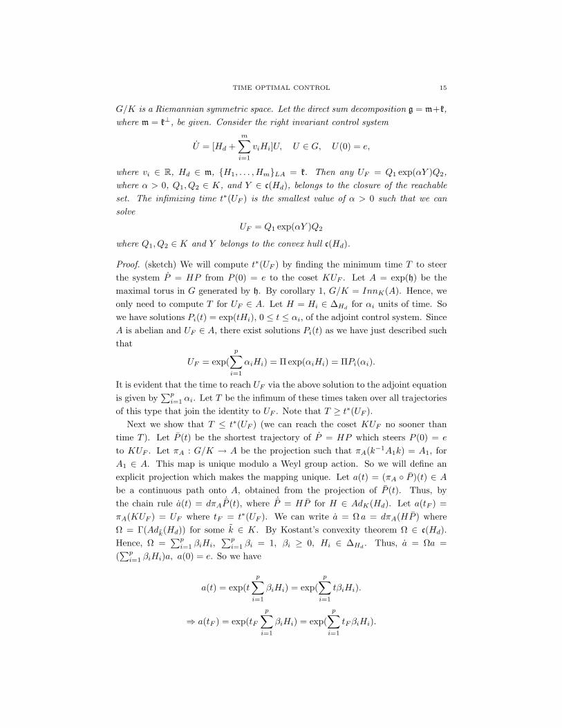
TIME OPTIMAL CONTROL 15
G/K is a Riemannian symmetric space. Let the direct sum decomposition g = m+k,where m = k⊥, be given. Consider the right invariant control system
U = [Hd +m∑i=1
viHi]U, U ∈ G, U(0) = e,
where vi ∈ R, Hd ∈ m, H1, . . . ,HmLA = k. Then any UF = Q1 exp(αY )Q2,where α > 0, Q1, Q2 ∈ K, and Y ∈ c(Hd), belongs to the closure of the reachableset. The infimizing time t∗(UF ) is the smallest value of α > 0 such that we cansolve
UF = Q1 exp(αY )Q2
where Q1, Q2 ∈ K and Y belongs to the convex hull c(Hd).
Proof. (sketch) We will compute t∗(UF ) by finding the minimum time T to steerthe system P = HP from P (0) = e to the coset KUF . Let A = exp(h) be themaximal torus in G generated by h. By corollary 1, G/K = InnK(A). Hence, weonly need to compute T for UF ∈ A. Let H = Hi ∈ ∆Hd for αi units of time. Sowe have solutions Pi(t) = exp(tHi), 0 ≤ t ≤ αi, of the adjoint control system. SinceA is abelian and UF ∈ A, there exist solutions Pi(t) as we have just described suchthat
UF = exp(p∑i=1
αiHi) = Π exp(αiHi) = ΠPi(αi).
It is evident that the time to reach UF via the above solution to the adjoint equationis given by
∑pi=1 αi. Let T be the infimum of these times taken over all trajectories
of this type that join the identity to UF . Note that T ≥ t∗(UF ).Next we show that T ≤ t∗(UF ) (we can reach the coset KUF no sooner than
time T ). Let P (t) be the shortest trajectory of P = HP which steers P (0) = e
to KUF . Let πA : G/K → A be the projection such that πA(k−1A1k) = A1, forA1 ∈ A. This map is unique modulo a Weyl group action. So we will define anexplicit projection which makes the mapping unique. Let a(t) = (πA P )(t) ∈ Abe a continuous path onto A, obtained from the projection of P (t). Thus, bythe chain rule a(t) = dπA
˙P (t), where ˙P = HP for H ∈ AdK(Hd). Let a(tF ) =πA(KUF ) = UF where tF = t∗(UF ). We can write a = Ω a = dπA(HP ) whereΩ = Γ(Adk(Hd)) for some k ∈ K. By Kostant’s convexity theorem Ω ∈ c(Hd).Hence, Ω =
∑pi=1 βiHi,
∑pi=1 βi = 1, βi ≥ 0, Hi ∈ ∆Hd . Thus, a = Ωa =
(∑pi=1 βiHi)a, a(0) = e. So we have
a(t) = exp(tp∑i=1
βiHi) = exp(p∑i=1
tβiHi).
⇒ a(tF ) = exp(tFp∑i=1
βiHi) = exp(p∑i=1
tFβiHi).

16 JODY-LYNN STORM
Note that for each Hi we have ‖Hi‖ = ‖H‖ = 1. Therefore, since∑pi=1 βi = 1,
we have
t∗(UF ) = tF =p∑i=1
tFβi ≥p∑i=1
αi = T.
4. Conclusion
In this paper, we presented a mathematical formulation of the problem of find-ing the shortest pulse sequences in NMR. We showed how the problem of comput-ing minimum time to produce a unitary propagator can be reduced to finding theshortest length paths on certain coset spaces. A remarkable feature of time optimalcontrol, and key to our results, is that the control is zero most of the time withpulses in between. We are now left with the open problem of computing minimumtime to produce a unitary propagator in the Chatter Sequence case. In this casethe coset space is no longer Riemannian Symmetric.
Note. As of May 8, 2006, the largest quantum information processor to be con-structed was based on a 12-qubit system (Science Daily), which is quite small. Thefollowing is a list of candidates for quantum computing that are currently beingexplored.
(1) Superconductor-based quantum computers (including SQUID-based quan-tum computers)
(2) Trapped ion quantum computer(3) Optical lattices(4) Topological quantum computer(5) Quantum dot on surface (e.g. the Loss-DiVincenzo quantum computer)(6) Nuclear magnetic resonance on molecules in solution (liquid NMR)(7) Solid state NMR Kane quantum computers(8) Electrons on helium quantum computers(9) Cavity quantum electrodynamics (CQED)
(10) Molecular magnet(11) Fullerene-based ESR quantum computer(12) Optic-based quantum computers (Quantum optics)(13) Diamond-based quantum computer(14) BoseEinstein condensate-based quantum computer(15) Transistor-based quantum computer - string quantum computers with en-
trainment of positive holes using a electrostatic trap(16) Spin-based quantum computer(17) Adiabatic quantum computation

TIME OPTIMAL CONTROL 17
The large number of candidates clearly shows that the topic is still in its infancy.
5. Appendix
The background needed to properly understand the control theory problem tooksome interesting turns, one of which was in the classification of compact Lie groups;a subject that deserves to be explored in greater detail. Thus, an in-depth studyof the classification of compact Lie groups has been added as an appendix to thispaper.
Representation.
Definition. A (finite dimensional) representation of a Lie group G is a continuoushomomorphism φ : G → Aut(V ), where V is a (finite dimensional) vector space.The dimension of the representation is the dimension of the vector space V . Denotethe representation of G in V by (G,V ).
Definition. Let (G,V ) be a representation. A subspace U of V is called invariantif gU ⊂ U for all g ∈ G.
Definition. A representation is called irreducible if the only invariant subspacesare 0 and V .
Definition. Two representations φ1 : G → Aut(V1) and φ2 : G → Aut(V2) aresaid to be equivalent (denoted by φ1
∼= φ2) if V1 and V2 are isomorphic, i.e., thereexists a linear isomorphism A : V1 → V2 such that A(φ1(g)(v)) = φ2(g)(A(v)), forall g ∈ G and v ∈ V1.
Hence the following diagram commutes:
V1
φ1(g) //
A
V1
A
V2
φ2(g) // V2
An automorphism of a Lie group G is a map φ : G→ G that is a diffeomorphismand a group homomorphism. Let G be a Lie group and let x ∈ G. Then the mapIx : G→ G sending each g to xgx−1 is a automorphism. Note that Ix = Rx−1 Lxis a diffeomorphism called an inner automorphism of G.
Definition. The adjoint representation of G is the homomorphism Ad : G →Aut(g) given by Ad(g) = (dIg)e.
Definition. The adjoint representation of g is the homomorphism ad : g→ End(g)given by ad(X) = (dAd)e(X).

18 JODY-LYNN STORM
Theorem 6. The adjoint representation of g satisfies ad(X)Y = [X,Y ] for allX,Y ∈ g.
Proposition 2. If G is a matrix group, then Ad(g)X = gXg−1 for all g ∈ G,X ∈ g.
Remark. If V is a vector space over R, then we can define the vector space
V C = V ⊗R C = X + iY : X,Y ∈ V, i =√−1
(or simply V⊗C), whose dimension over C equals the dimension of V over R. Ifg is a Lie bracket over R, then the complexification of g is the Lie algebra g ⊗ C(sometimes written as g + ig), with the bracket operation given by
[U + iV,X + iY ] = [U,X]− [V, Y ] + i([V,X] + [U, Y ]).
Example. Let G = SU(2) with Lie algebra g = su(2) consisting of matrices of the
form
(iα z
−z −iα
).
Let A =
(x+ iy u+ iv
−u+ iv x− iy
)∈ SU(2). We need to compute Ad : SU(2) →
Aut(su(2)), the linear transformation given by Ad(A)B = ABA−1. Let
E1 =
(i 00 −i
), E2 =
(0 1−1 0
), E3 =
(0 i
i 0
)be a basis for su(2). Calculating Ad(A)E1 gives
Ad
(x+ iy u+ iv
−u+ iv x− iy
)(i 00 −i
)=
(x+ iy u+ iv
−u+ iv x− iy
)(i 00 −i
)(x− iy −u− ivu− iv x+ iy
)
=
(ix2 + iy2 − iu2 − iv2 −2ixu+ 2uy + 2xv + 2iyv
2iux+ 2xv − 2uy + 2ivy iu2 + iv2 − ix2 − iy2
)
By computations on the other basis elements we get
Ad
(x+ iy u+ iv
−u+ iv x− iy
)=
x2 + y2 − u2 − v2 −2xv + 2uy 2xu+ 2yv2uy + 2xv x2 − y2 + u2 − v2 −2xy + 2uv−2xu+ 2yv 2xy + 2uv x2 − y2 − u2 + v2
Notice that this is a 3× 3 matrix, which agrees with the dimension of the repre-sentation which is dim(su(2)) = 3

TIME OPTIMAL CONTROL 19
Standard representation. We will define the standard representations ofGL(n,R),O(n) and SO(n) on Mn×1R ∼= Rn with the operation being matrix multiplicationon Rn, i.e., φ(g)v = gv. Similarly we can define the standard representations ofGL(n,C), SU(n) and U(n) on Mn×1C ∼= Cn with the operation being matrix mul-tiplication on Cn. Let λn denote the standard representation of GL(n,R) and letλn denote the standard representation of SO(n) (or O(n)). Let µn denote the stan-dard representation of GL(n,C) and let µn denote the standard representation ofSU(n)(or U(n)). Let vn denote the standard representation of Sp(n). A repre-sentation is called trivial, denoted by 1, if each group element acts as the identitytransformation. Then the adjoint representations of these groups are equivalent tothe following representations:
AdGL(n,R) = λn ⊗R λ∗n,
AdGL(n,C) = µn ⊗C µ∗n,
AdSO(n) = ∧2λn,
AdU(n) ⊗ C = µn ⊗C µ∗n = µn ⊗C µn,
AdSU(n) ⊗ C = µn ⊗C µn − 1,
AdSp(n) ⊗ C = S2vn
For a better understanding of the above equivalences, we will show thatAdGL(n,R) =λn ⊗R λ
∗n. Note that GL(n,R) ∼= Aut(Rn) and for A ∈ GL(n,R), x ∈ Rn we
have λn(A)x = Ax. Since Rn and (Rn)∗ are finite vector spaces, Rn ⊗ (Rn)∗ ∼=Hom(Rn,Rn) = gl(n) by the mapping Rn ⊗ (Rn)∗ → Hom(Rn,Rn) defined by(w⊗ θ)v = θ(v)w. Thus we need to find an isomorphism φ which makes the follow-ing diagram commute
Rn ⊗ (Rn)∗λn⊗λ∗n(g)
//
φ
Rn ⊗ (Rn)∗
φ
gl(n)
Ad(g) // gl(n)
First consider the case when n = 2. Then we have the following maps:
λ2 : GL(2,R)→ Aut(R2),
λ∗2 : GL(2,R)→ Aut(R2),
λ2 ⊗ λ∗2 : GL(2,R)→ Aut(R2 ⊗ (R2)∗)
where v ∈ R2 is a column vector and u ∈ (R2)∗ a row vector. Choose the standardbasis
20 JODY-LYNN STORM
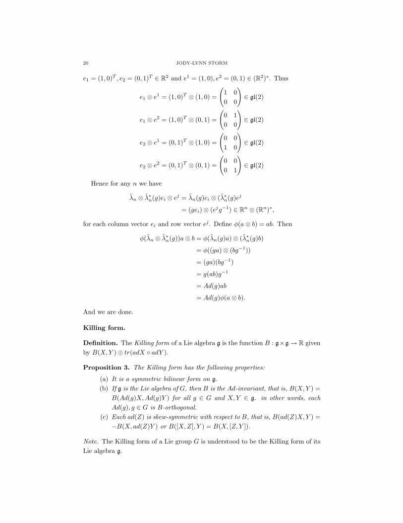
e1 = (1, 0)T , e2 = (0, 1)T ∈ R2 and e1 = (1, 0), e2 = (0, 1) ∈ (R2)∗. Thus
e1 ⊗ e1 = (1, 0)T ⊗ (1, 0) =
(1 00 0
)∈ gl(2)
e1 ⊗ e2 = (1, 0)T ⊗ (0, 1) =
(0 10 0
)∈ gl(2)
e2 ⊗ e1 = (0, 1)T ⊗ (1, 0) =
(0 01 0
)∈ gl(2)
e2 ⊗ e2 = (0, 1)T ⊗ (0, 1) =
(0 00 1
)∈ gl(2)
Hence for any n we have
λn ⊗ λ∗n(g)ei ⊗ ej = λn(g)ei ⊗ (λ∗n(g)ej
= (gei)⊗ (ejg−1) ∈ Rn ⊗ (Rn)∗,
for each column vector ei and row vector ej . Define φ(a⊗ b) = ab. Then
φ(λn ⊗ λ∗n(g))a⊗ b = φ(λn(g)a)⊗ (λ∗n(g)b)
= φ((ga)⊗ (bg−1))
= (ga)(bg−1)
= g(ab)g−1
= Ad(g)ab
= Ad(g)φ(a⊗ b).
And we are done.
Killing form.
Definition. The Killing form of a Lie algebra g is the function B : g×g→ R givenby B(X,Y )⊕ tr(adX adY ).
Proposition 3. The Killing form has the following properties:
(a) It is a symmetric bilinear form on g.(b) If g is the Lie algebra of G, then B is the Ad-invariant, that is, B(X,Y ) =
B(Ad(g)X,Ad(g)Y ) for all g ∈ G and X,Y ∈ g. in other words, eachAd(g), g ∈ G is B-orthogonal.
(c) Each ad(Z) is skew-symmetric with respect to B, that is, B(ad(Z)X,Y ) =−B(X, ad(Z)Y ) or B([X,Z], Y ) = B(X, [Z, Y ]).
Note. The Killing form of a Lie group G is understood to be the Killing form of itsLie algebra g.

TIME OPTIMAL CONTROL 21
Definition. (semisimple) A Lie group G is called semisimple if its Killing formis non-degenerate.
We can think of a semisimple Lie algebra g as one that has no proper subspaceh with [X,Y ] = 0 if X ∈ h and Y ∈ g.
Theorem 7. If G is a compact semisimple Lie group, then its Killing form isnegative definite, i.e., B(X,X) < 0 for all X 6= 0 in G.
Example. To compute the Killing form of SU(2) it is sufficient to compute the
Killing form on its Lie algebra su(2). Let X =
(iθ 00 −iθ
), Y =
(iφ 00 −iφ
)∈
su(2) and consider the basis
(i 00 −i
),
(0 1−1 0
),
(0 i
i 0
)of su(2). Then adX =0 0 0
0 0 −2θ0 2θ 0
and adY =
0 0 00 0 −2φ0 2φ 0
. So
B(X,Y ) = tr(ad(X)ad(Y )) = tr
0 0 00 −4θφ 00 0 −4θφ
= −8θφ = 4trXY.
Example. As with SU(2), to compute the Killing form of U(2) we compute theKilling form of u(2) with the following basis:(
i 00 0
),
(0 00 i
),
(0 1−1 0
),
(0 i
i 0
).
Let X =
(iθ1 00 −iθ2
)and Y =
(iφ1 00 −iφ2
)∈ u(2). Then
adX =
0 0 0 00 0 0 00 0 0 θ1 − θ20 0 −θ1 − θ2 0
, adY =
0 0 0 00 0 0 00 0 0 φ1 − φ2
0 0 −φ1 − φ2 0
.
ThusB(X,Y ) = tr(adX, adY ) = tr
0 0 0 00 0 0 00 0 −(θ1 − θ2)(φ1 + φ2) 00 0 0 −(θ1 + θ2)(φ1 − φ2)
=
4(θ1φ1 + θ2φ2)− 2(θ1 + θ2)(φ1 + φ2) = 4trXY − 2trXtrY.Notice that if θ1 = θ2 = φ1 = φ2 = 1, then B(X,Y ) = 0. So U(2) is not semisimple.
Example. As in the previous examples, to compute the Killing form of SO(3) weonly need to compute the Killing form of so(3). Consider the following basis of

22 JODY-LYNN STORM
so(3):
E1 =
0 1 0−1 0 00 0 0
, E2 =
0 0 10 0 0−1 0 0
, E3 =
0 0 00 0 10 −1 0
.
Since tr(adEiadEj) = 0 for i 6= j, it suffices to compute the Killing form for thematrices
X =
0 θ 0−θ 0 00 0 0
, Y =
0 φ 0−φ 0 00 0 0
.
in so(3). So we have
adX =
0 0 00 0 θ
0 −θ 0
, adY =
0 0 00 0 φ
0 −φ 0
ThusB(X,Y ) = tr
0 0 0
0 0 θ
0 −θ 0
0 0 0
0 0 φ
0 −φ 0
= tr
0 0 00 −θφ 00 0 −θφ
= −2θφ =
trXY.
By generalizing the above examples we obtain the following formulas:
U(n) : B(X,Y ) = 2ntrXY − 2trXtrY,
SU(n) : B(X,Y ) = 2ntrXY,
SO(n) : B(X,Y ) = (n− 2)trXY,
Sp(n) : B(X,Y ) = 2(n+ 1)trXY.
Maximal tori.
Definition. (torus) A torus in a Lie group G is a Lie subgroup that is isomorphicto a product of S1 × ...× S1. A torus T is a maximal torus in G if for any torus Sin G with T ⊂ S ⊂ G, then T = S.
Example. The set T =
(eiθ 00 e−iθ
)is a maximal torus in SU(2).
Remark.
• Any torus is contained in a maximal torus.• If G is compact then any maximal torus T is a maximal connected abelian
subgroup of G.

TIME OPTIMAL CONTROL 23
• If T is a connected subgroup of a compact Lie group G whose Lie algebrais a maximal abelian subalgebra of g, then T is a maximal torus in G.
Theorem 8. Let G be a compact and connected Lie group. Then:
(a) Any element in G is contained in some maximal torus.(b) Any two maximal tori are conjugate. That is, if T1, T2 are maximal tori
in G, then there exists an element g ∈ G such that gT1g−1 = T2.
From the above theorem we can conclude that all maximal tori have the samedimension, so is an invariant for a compact and connected Lie group.
Definition. (rank) The rank of a compact and connected Lie group is the dimen-sion of a maximal torus.
Proposition 4. Let G be a compact and connected Lie group with Lie algebra g.Then:
(a) The exponential map is onto.(b) There is a one-to-one correspondence between maximal tori T in G and
maximal abelian subspaces h in g given by T ↔ h = exp t, where t is theLie algebra of T .
(c) If T is a maximal torus in G with Lie algebra t, then G = ∪g∈GgTg−1
and g = ∪g∈GAd(g)t.(d) The center of G is equal to ∩maximaltoriT .(e) If S is a subset of G, we define the centralizer of S to be the set C(S) =g ∈ G : gx = xgforallx ∈ S. Then, if T is a maximal torus in G,C(T ) = T .
(f) Maximal tori are also maximal abelian subgroups.(g) For any X ∈ g, the closure of exp(tX) is a compact abelian subgroup
of G, and hence is a torus.
Example. Consider the set T = diag(eiθ1 , . . . , eiθn). Clearly T is a torus in U(n).Let A ∈ U(n) such that AT = TA. Let TJ be the subgroup of matrices tj with 1 onthe jth entry and 0 elsewhere. Then, for all tj ∈ Tj we have tjAej = Atjej = Aej ,where ej is the column vector with 1 in the jth place and 0 elsewhere. Since A isfixed by T , there exists some λj ∈ C such that Aej = λjej . Also, A ∈ U(n), thusλj has modulus 1. Therefore λj = eiφj for some φ. Since this is true for each j,A = diag(eiφ1 , . . . , eiφn). Thus A ∈ T and T is a maximal torus in U(n) and therank of U(n) is n.
Classification of compact and connected Lie groups. All the groups in thissection are assumed to be compact and connected.
Definition. A Lie group is called simple if it is non-abelian and it does not containany proper normal Lie subgroups. Equivalently, a Lie group is simple if its Liealgebra is simple, i.e. it is non-abelian and has no proper ideals.

24 JODY-LYNN STORM
Note. The above definition gives a correspondence between normal subgroups andideals.
Theorem 9.
(a) Let G be a compact and connected Lie group. Then there exists a cover-ing space of G that is isomorphic to the direct product of a torus and acompact, connected and simply connected Lie group.
(b) Every compact, connected and simply connected Lie group is isomorphico the direct product of simple, compact, connected and simply connectedLie groups.
(c) The simple, compact, connected and simply connected Lie groups are thefollowing:
SU(n)(≥ 2), SO(2n+ 1)(n ≥ 3), Sp(n)(n ≥ 2), SO(2n)(n ≥ 4), G2, F4, E6, E7, E8.
Remark. The Lie algebras of the first four groups are denoted by An−1, Bn, Cn, Dn
respectively. The following isomorphisms hold: A1∼= B1
∼= C1, B2∼= C2, A3
∼=D3, D2
∼= A1 ⊕ A1. The last five Lie groups are called the exceptional Lie groups.Their indices indicate the rank of the group and their dimensions are 14, 52, 78,133 and 248 respectively.
Complex semisimple Lie algebras. A simply connected Lie group is determinedby its Lie algebra, so there is a one-to-one correspondence (up to isomorphism) be-tween compact semisimple Lie algebras and compact Lie groups. By complexifyingthese Lie algebras we obtain a one-to-one correspondence between these complexi-fied Lie algebras and the complex semisimple Lie algebras. The complex semisimpleLie algebras are classified by their root systems, and the root systems are classi-fied by their bases. The bases are described by the Dynkin diagrams. Hence, inthis section, we end up with a one-to-one correspondence between compact simplyconnected Lie groups and Dynkin diagrams.
Definition. Let g be a complex Lie algebra.
(1) The adjoint representation of g is the homomorphism ad : g → End(g)given by ad(X)(Y ) = [X,Y ] for all X,Y ∈ g.
(2) The Killing form of g is the symmetric bilinear form given by B(X,Y ) =tr(adX adY ), (X,Y ∈ g).
(3) g is called semisimple if its Killing form is non-degenerate.(4) g is called simple if it is non-abelian and its only ideals are 0 and g.(5) A Cartan subalgebra h of g is a maximal abelian subalgebra of g such that,
for all H ∈ h the endomorphism ad(h) is diagonalizable.
Proposition 5. A Lie algebra is semisimple if and only if it is isomorphic to aproduct of simple Lie algebras.

TIME OPTIMAL CONTROL 25
Proposition 6.
(a) Any complex Lie algebra contains a Cartan subalgebra.(b) Let G be the group of automorphisms of g generated by the following
elements:
exp(adX) =∞∑n=0
1n!
(adX)n, (X ∈ g)
Then any two Cartan subalgebras are conjugate under G. This group iscalled the adjoint group.
Note. If G is a compact Lie group with Lie algebra g, and h1, h2 are two Cartansubalgebras of g, then there exists a g ∈ G such that Ad(g)h1 = h2.
Definition. The rank of a Lie algebra is the dimension of a Cartan subalgebra.
Let g be a complex semisimple Lie algebra and h a fixed Cartan subalgebra of g.Let h∗ be the dual space of h. Then for all α ∈ h∗, let gα = X ∈ g : ad(H)X =α(H)X for all H ∈ h denote the corresponding eigenspace of g. If α ∈ h∗ suchthat α 6= 0 and gα 6= 0, then we call α a root of g. We call gα the root spacecorresponding to α. Denote the set of all the roots of g by R, called the root systemof g (relative to h). In particular, let g0 be the set of all elements of g that commutewith h. Since h is maximal abelian, g0 = h. Also. for all H ∈ h, the endomorphismsad(H) are diagonalizable and commute, so they are simultaneously diagonalizable.Thus, for a fixed h we obtain the root space decomposition of g
g = h⊕∑α∈R
gα
For each α ∈ R, let Hα denote the unique element in h such that B(Hα, H) = α(H)for all H ∈ h. This called the root vector for α.
Proposition 7.
(a) If α is a root, then so is −α.(b) The roots span h∗ and the root vectors span h.(c) [gα, gβ ] ⊂ gα+β. If α+ β /∈ R the bracket is interpreted as 0.(d) The killing form is non-degenerate on h.(e) The subspace [gα, g−α] of h has dimension 1. Let Eα ∈ gα and E−α ∈
g−α. Then [Eα, E−α] = B(Eα, E−α)Hα.(f) For each α ∈ R the dimension of each gα is 1.(g) If α ∈ R and kα ∈ R for some integer k, the k = ±1.
Elements Eα of gα with [Eα, E−α] = Hα are called root elements. Let hR =∑α RHα.

26 JODY-LYNN STORM
Example. Consider the Lie algebra sl(3,C) = A ∈ M3C : trA = 0 with thefollowing basis:
H1 =
1 0 00 0 00 0 −1
, H2 =
0 0 00 1 00 0 −1
,
X1 =
0 1 00 0 00 0 0
, X2 =
0 0 10 0 00 0 0
, X3 =
0 0 00 0 10 0 0
,
X4 =
0 0 01 0 00 0 0
, X5 =
0 0 00 0 01 0 0
, X6 =
0 0 00 0 00 1 0
The diagonal matrices H1, H2 form a basis for the Cartan subalgebra h of sl(3,C).The dimension of sl(3,C) is 8. The rank of sl(3,C) is the dimension of h, which is2. Hence the roots of sl(3,C) are ordered pairs α = (α1, α2) ∈ C2. Moreover, if Xis a root vector, then X is a simultaneous eigenvector for ad(H1) and ad(H2) i.e.,[H1, X] = α1X and [H2, X] = α2X. Below we have the bracket table of the basiselements.
[ , ] H1 H2 X1 X2 X3 X4 X5 X6
H1 0 0 X1 2X2 X3 −X4 −2X5 −X6
H2 0 0 −X1 X2 2X3 X4 −X5 −2X6
X1 −X1 X1 0 0 X2 H1 −H2 −X6 0X2 −2X2 −X2 0 0 0 −X3 H1 X1
X3 −X3 −2X3 −X2 0 0 0 X4 H2
X4 X4 −X4 −H1 +H2 X3 0 0 −X5 0X5 2X5 X5 X6 −H1 −X4 0 0 0X6 X6 2X6 0 −X1 −H2 X5 0 0
By the above table we have the following roots of sl(3,C) with correspondingroot vectors, where each root vector Xi is the span of the corresponding root spacesgαi .
TIME OPTIMAL CONTROL 27
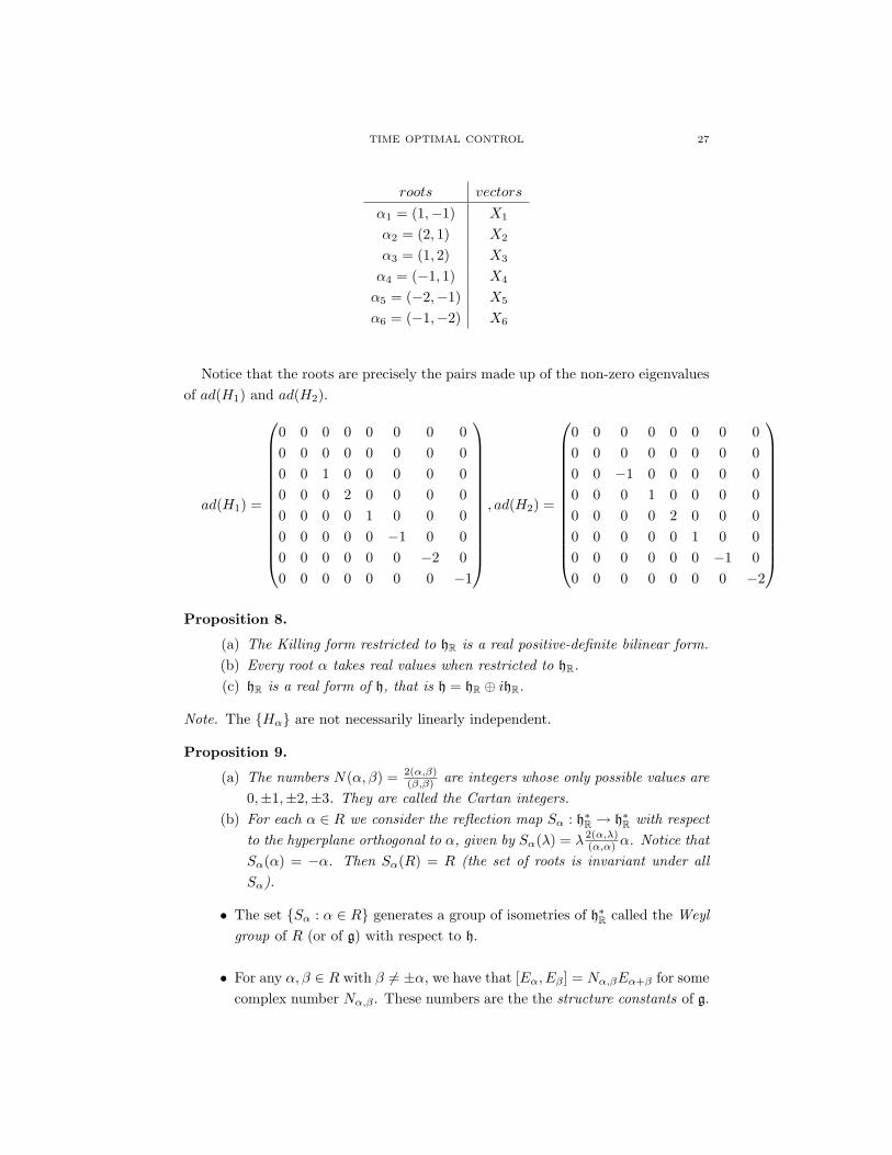
roots vectors
α1 = (1,−1) X1
α2 = (2, 1) X2
α3 = (1, 2) X3
α4 = (−1, 1) X4
α5 = (−2,−1) X5
α6 = (−1,−2) X6
Notice that the roots are precisely the pairs made up of the non-zero eigenvaluesof ad(H1) and ad(H2).
ad(H1) =
0 0 0 0 0 0 0 00 0 0 0 0 0 0 00 0 1 0 0 0 0 00 0 0 2 0 0 0 00 0 0 0 1 0 0 00 0 0 0 0 −1 0 00 0 0 0 0 0 −2 00 0 0 0 0 0 0 −1
, ad(H2) =
0 0 0 0 0 0 0 00 0 0 0 0 0 0 00 0 −1 0 0 0 0 00 0 0 1 0 0 0 00 0 0 0 2 0 0 00 0 0 0 0 1 0 00 0 0 0 0 0 −1 00 0 0 0 0 0 0 −2
Proposition 8.
(a) The Killing form restricted to hR is a real positive-definite bilinear form.(b) Every root α takes real values when restricted to hR.(c) hR is a real form of h, that is h = hR ⊕ ihR.
Note. The Hα are not necessarily linearly independent.
Proposition 9.
(a) The numbers N(α, β) = 2(α,β)(β,β) are integers whose only possible values are
0,±1,±2,±3. They are called the Cartan integers.(b) For each α ∈ R we consider the reflection map Sα : h∗R → h∗R with respect
to the hyperplane orthogonal to α, given by Sα(λ) = λ 2(α,λ)(α,α) α. Notice that
Sα(α) = −α. Then Sα(R) = R (the set of roots is invariant under allSα).
• The set Sα : α ∈ R generates a group of isometries of h∗R called the Weylgroup of R (or of g) with respect to h.
• For any α, β ∈ R with β 6= ±α, we have that [Eα, Eβ ] = Nα,βEα+β for somecomplex number Nα,β . These numbers are the the structure constants of g.

28 JODY-LYNN STORM
Recall that the cosine of the angle θ between α and β in Euclidean space is givenby the formula ‖α‖‖β‖ cos θ = (α, β). Thus, N(β, α) = 2 ‖β‖‖α‖ and N(α, β)N(β, α) =4 cos2 θ ≥ 0. Also, notice that N(α, β) and N(β, α) have the same sign, so thefollowing are the only possibilities for angles and relative lengths when α 6= ±β and‖β‖ ≥ ‖α‖.
N(α, β) N(β, α) θ ‖β‖2/‖α‖2
0 0 π/2 undetermined
1 1 π/3 1−1 −1 2π/3 11 2 π/4 2−1 −2 3π/4 21 3 π/6 3−1 −3 5π/6 3
A reduced root system of rank 1 is called A1. It consists of a pair of vectors,±α. There are four non-isomorphic reduced root systems of rank 2; A1 × A1, A2,B2 and G2 (see theorem 9 and the following remark), represented by the followinggraphs. Notice that the root system of sl(3,C) in the above example correspondsto the graph of A2.

TIME OPTIMAL CONTROL 29

30 JODY-LYNN STORM
Proposition 10. For α, β, γδ ∈ R we have the following:
(a) Nα,β = −Nβ,α.(b) Nα,β = Nβ,γ = Nγ,α for α+ β + γ = 0(c) Nα,βNγ,δ +Nα,γNδ,β +Nα,δNβ,γ = 0 for α+ β + γ + δ = 0.(d) α+ β is a root if and only if Nα,β 6= 0.(e) It is possible to choose the root elements Eα in such a way so that the
structure constants are real numbers satisfying Nα,β = −N−α,−β.(f) (Chevalley) The structure constants can be chosen to be integers.
Definition. Let g be a complex semisimple Lie algebra with h a Cartan subalgebra,and root system R. Let H1, . . . ,Hl (l =rank of g) be a basis for h. For each α ∈ Rlet Eα be root elements satisfying Eα, E−α] = Hα, and such that the structureconstants are integers with Nα,β = −N−α,−β . Then the set H1, . . . ,Hl;Eα : α ∈R is said to be a Weyl-Chevalley basis for g.
Proposition 11. Let R be the root system of a complex semisimple Lie alge-bra g(with respect to a fixed Cartan subalgebra). Then there exists a subset Π =α1, . . . , αl (l =rank of g) such that every root α ∈ R can be expressed uniquely asα1α1 + . . .+ nlαl, where ni are integers, either all positive or all negative.
We call Π a set of simple roots for R. Π is called irreducible if there is nonontrivial disjoint union Π = Π1 ∪Π2 with (α, β) = 0 for all α ∈ Π1 and β ∈ Π2.
A root is called positive (α > 0) if α =∑li=1 niαi with all ni ≥ 0. Let R+ denote
the set of positive roots and let R− = −α : α ∈ R+.
Proposition 12. R+ is called an ordering in R and satisfies the following:

TIME OPTIMAL CONTROL 31
(a) R+ ∩ (−R+) = ∅, R+ ∪ (−R+) = R.(b) For each α, β ∈ R+ with α+ β ∈ R+, i.e, for each α, β ∈ R, then α > β
if and only if α− β ∈ R+.
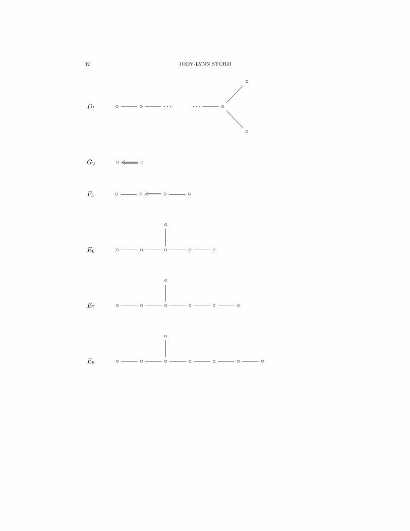
Definition. The Dynkin diagram of a root system R with a set of simple roots Πconsists of a planar graph with l vertices labeled with α1, . . . , αl andN(αi, αj)N(αj , αi)line segments joining the vertex αi to the vertex αj . If N(α, β) > 0 and (β, β) >(α, α), draw an arrow on the line segment from the vertex of β (long root) to thevertex from the vertex of α (short root).
Theorem 10. Classification Assigning to each complex semisimple Lie algebra theDynkin diagram of the root system of a Cartan subalgebra, sets up a one-to-onecorrespondence between the set of such Lie algebras (up to isomorphism) and fun-damental root systems (up to equivalence). In particular, the simple Lie algebrascorrespond to irreducible fundamental systems.
The following is a list of the complex Lie algebras along with their Dynkin dia-grams
Name Description Rank Dimension
Al sll+1C l ≥ 1 l(l + 2)Bl so2l+1C l ≥ 2 l(2l + 1)Cl splC l ≥ 3 l(2l + 1)Dl so2lC l ≥ 4 l(2l + 1)G2 −− 2 14F4 −− 4 52E6 −− 6 78E7 −− 7 133E8 −− 8 248
Al . . . . . .
Bl . . . . . . +3
Cl . . . . . . ks
32 JODY-LYNN STORM
Dl . . . . . .
>>>>>>>>
G2 _jt
F4 ks
E6
E7
E8

TIME OPTIMAL CONTROL 33
Definition. A real Lie algebra g0 is called a real form of a complex Lie algebra g,if g is isomorphic to the complexification of g0, that is, g = g0 + ig0.
Remark. (Weyl) Every complex semisimple Lie algebra has a compact real form.Compact means that its Killing form is negative definite. All compact real forms ofg are conjugate via an inner automorphism.
Any real form gR can be characterized as a fixed point set of a conjugate linearinvolution τ : g→ g (τ2 = I, τ is linear over the reals), which is an automorphism ofg considered as a real Lie algebra. If g = h⊕
∑α∈R gα is a root space decomposition
of g, then we can construct a compact real form g0 of g by the conjugate linear mapτ0 : g→ g defined by
τ |hR = −Id, τ(Eα) = −E−α.
This is called the standard involution associated with the root space decomposition.The set of fixed points of τ is the compact real form given by
g0 = ihR ⊕⊕α∈R+
R(Eα − E−α ⊕⊕α∈R+
Ri(Eα + E−α)
The elements of iHα, Eα − E−α, iEα + E−α generate a subalgebra of g isomorphicto su(2) given by
iHα 7→
(1 00 −1
), Eα − E−α 7→
(0 1−1 0
), Eα + E−α 7→
(0 −ii 0
),
We can also use the root spaces to obtain homomorphisms into sl(C given by
iHα 7→
(1 00 −1
), Eα 7→
(0 10 0
), E−α 7→
(0 01 0
).

34 JODY-LYNN STORM
References
[1] Andreas Arvanitoyeorgos, An Introduction to Lie Groups and the Geometry of Homogeneous
Spaces. American Mathematical Society, 2003.
[2] Brian C. Hall, Lie Groups, Lie Algebras, and Representations: An Elementary Introduction.
Springer Science+Business Media, 2003.
[3] James E. Humphreys, Introduction to Lie Algebras and Representation Theory. Springer-
Verlag, 1972.
[4] N. Khaneja, R. Brocktett, and S. Glaser, ”‘Time Optimal Control of Spin Systems”’, Phys.
Rev. A, 63, 032308, 2001.
[5] Navin Khaneja, Geometric Control in Classical and Quantum Systems (Ph.d Thesis, Harvard
University, 2000).
[6] Kobayashi, S., and Nomizu, K., Foundations of Differential Geometry Vol.1 and 2. Inter-
science Publishers, 1969.
[7] Richard W. Sharpe, Differential Geometry: Cartan’s Generalization of Klein’s Erlangen Pro-
gram. Springer-Verlag, 1997.
Mathematics Department, University of Hawai‘i, Manoa, 2565 The Mall, Honolulu,
HI 96822
E-mail address: [email protected]