time-lapse imaging - imagescience.org · meijering et al. 1/32 time-lapse imaging time-lapse...
TRANSCRIPT

Meijering et al. 1/32 Time-Lapse Imaging
Time-Lapse Imaging
Erik Meijering, Ihor Smal, Oleh Dzyubachyk,
Jean-Christophe Olivo-Marin
Chapter 15 of Microscope Image Processing
Q. Wu, F. A. Merchant, K. R. Castleman (eds.)
Elsevier Academic Press, 2008, pp. 401-440
INTRODUCTION
By their very nature, biological systems are dynamic, and a proper understanding of the cellular and
molecular processes underlying living organisms and how to manipulate them is a prerequisite to com-
bat diseases and improve human health care. One of the major challenges of current biomedical re-
search, therefore, is to unravel not just the spatial organization of these complex systems, but their spa-
tiotemporal relationships [142,42]. Catalyzed by substantial improvements in optics hardware, elec-
tronic imaging sensors, and a wealth of fluorescent probes and labeling methods, light microscopy has,
over the past decades, matured to the point that it enables sensitive time-lapse imaging of cells and
even single molecules [150,93,166,100]. These developments have had a profound impact on how re-
search is currently being conducted in the life sciences.
An inevitable consequence of the new opportunities offered by these developments is the fact that the
size and complexity of image data is ever increasing. Nowadays, data sets generated in time-lapse ex-
periments commonly comprise hundreds to thousands of images, each containing hundreds to thou-
sands of objects to be analyzed (see Figure 1 for examples). Needless to say, such huge amounts of data
cannot be digested by visual inspection or manual processing within any reasonable amount of time. It
is now generally recognized that automated methods are necessary, not only to handle the growing rate
at which images are acquired, but, possibly even more importantly, to provide a level of sensitivity and
objectivity that human observers cannot match [97,41].
Roughly speaking, time-lapse imaging studies consist of four successive steps: 1) planning of the ex-
periment and acquisition of the image data, 2) preprocessing of the data to correct for systemic as well
as random errors and to enhance relevant features, 3) analysis of the data by detecting and tracking the
objects relevant to the biological questions underlying the study, and 4) analysis of the resulting tra-
jectories to test predefined hypotheses or detect new phenomena. This chapter addresses each of these
issues (see Figure 2 for a topical overview), from an informatics perspective. It focuses on meth-
odological rather than hardware or software aspects. It gives examples of image processing and analy-
sis methods that have been used successfully for specific applications. The ultimate goal of this chapter
is to prepare the reader to select methods intelligently.
IMAGE ACQUISITION
Time-lapse imaging experiments involve the acquisition of not only spatial information, but also tem-
poral information, and often spectral information as well, resulting in up to five-dimensional (5D) im-

Meijering et al. 2/32 Time-Lapse Imaging
age data sets (Figure 3). Regardless of the imaging technique used, a careful design of the microscope
setup is imperative, as shortcomings may require additional pre- or postprocessing of the resulting im-
age data or, worse, may lead to artifacts that cannot be removed and that may hamper data analysis.
While it is outside the scope of this chapter to provide detailed guidelines for establishing the right set-
up, a few general remarks are made here, concerning the choice of microscopy, spatial dimensionality,
and temporal resolution, from the perspective of subsequent data analysis.
Microscope Setup
A fundamental concern in time-lapse imaging experiments, which generally involve living cells and
organisms, is to keep the specimen alive during the acquisition of hundreds or thousands of images
over an extended period of time, ranging from minutes to hours, depending on the research question.
This not only calls for a suitable environment, with controlled temperature, humidity, and a stably
buffered culture medium [49], it also requires economizing light exposure, as living cells are sensitive
to photodamage [133]. In the case of fluorescence microscopy, illumination bleaches fluorophores,
which limits their emission time span and generates free radicals that are toxic for cells.
From an image analysis perspective, on the other hand, two very important factors that determine
whether automated methods can be successfully applied, and that strongly affect their accuracy, are
signal contrast (the difference in intensity between objects and background) and noise (which in light
microscopy is signal dependent). These two factors are usually combined into a single measure: the
signal-to-noise ratio (SNR). Ideally, experiments should be designed so as to maximize this measure in
order to allow robust and accurate automated image analysis, and the only way to accomplish this
would be to maximize light exposure and capture.
These contradictory requirements call for a careful choice of the type of microscopy to be used. This
also depends on the type of objects to be studied, their dimensions, motility, and viability. Living cells
in culture media, for example, produce poor contrast with standard brightfield illumination and often
require contrast enhancing imaging techniques, such as phase-contrast or differential interference con-
trast microscopy. Intracellular particles are hardly (if at all) visible without contrast enhancement and
are better studied using fluorescence microscopy (cf. Tables 1 and 2). Needless to say, in all cases the
system should make the best possible use of the available light, implying the use of high numerical ap-
erture objectives in conjunction with highly sensitive detectors. In many cases this may also mean that
widefield microscopy is preferable over confocal microscopy [133,49,78], with the proviso that 3D
widefield microscopy requires images to be deconvolved.
In practice, for any biological application, there is often no single best microscope setup. This means
that a compromise will have to be found between sufficient (but not toxic) illumination, and (spatial
and temporal) resolution, so that the maximum number of acceptable images (optical slices and time
frames) can be acquired before the specimen is completely photobleached or damaged [49], where “ac-
ceptable” means having the minimum SNR required by automated image analysis techniques (dis-
cussed later in this chapter). To this end, a good understanding of different microscope systems is
needed, for which we refer to excellent introductory texts [100].
Spatial Dimensionality
One of the fundamental questions to be addressed when setting up an experiment is whether imaging
needs to be performed in two or in three spatial dimensions over time (denoted as 2D+t and 3D+t, re-
spectively, the latter of which is also referred to as 4D). Despite the 4D imaging buzz in the literature,

Meijering et al. 3/32 Time-Lapse Imaging
the vast majority of experiments today are still performed in 2D+t (cf. Tables 1 and 2). Often, this is
due to limitations imposed by photobleaching and phototoxicity, which do not permit wasting light
signal, as occurs in confocal microscopy imaging. In other studies, in particular those addressing intra-
cellular dynamic processes, acquiring multiple optical slices would simply take too much time relative
to the motions of interest, resulting in intrascan motion artifacts. In some cases, for example when
studying cell migration in monolayers [64], or microtubule dynamics in neurons [132], the structures of
interest may be sufficiently flat to allow 2D+t imaging by widefield microscopy to give a good under-
standing of a process. The improved light collection and the lower number of optical slices in such cas-
es yields a better SNR and allows for higher temporal resolution.
Most cellular and intracellular processes, however, occur in three dimensions over time, and require
3D+t imaging in order to obtain a complete picture and fully characterize cell morphodynamics [133].
It is known, for example, that tumor cells treated with drugs that block migration on 2D substrates can
move inside an artificial 3D collagen matrix by means of a very different type of motility [152,166].
Regarding intracellular processes, studies into kinetochore microtubule dynamics [35] have recently
revealed that trajectories obtained from 2D+t imaging may differ significantly from those obtained
from 3D+t imaging and may lead to severe misinterpretation of the underlying processes. These find-
ings suggest that a paradigm shift may be necessary, in that 2D+t imaging studies should always be
preceded by 3D+t experiments confirming their validity. This could be as important as making sure
that fluorescent probes, in fluorescence microscopy imaging, do not alter physiology.
Temporal Resolution
Another issue of great importance in time-lapse experiments is the rate at which images should be ac-
quired over time, also referred to as the temporal sampling rate, or temporal resolution. Ideally, this
should be sufficiently high to capture the relevant details of object motion. However, similar to spatial
dimensionality and resolution, the temporal sampling rate is not an independent parameter that can be
fixed to any desired value, but is constrained by the limited viability of living cells under illumination.
Nevertheless, in view of eventual data analysis, it is important to be aware of possible discrepancies
between theoretically desirable and practically feasible values.
From sampling theory [123] it is known that in order to be able to reconstruct a continuous signal from
a digitized version of it, the latter must have been acquired by sampling at a rate that is at least twice
the maximum frequency component contained in the former. Similar to sampling in space (discussed in
detail elsewhere in this volume), this rate, often called the Nyquist rate, also applies to sampling in
time: true object position as a function of time is a continuous signal, and high-fidelity reconstruction
of this signal and any derivative motion parameters, such as velocity and acceleration, is possible only
if sampling is done at a rate that complies with theory.
Establishing this rate, however, is a chicken-and-egg problem: before sampling, one must already have
knowledge of the velocities to be estimated, which can only be obtained by sampling at a proper rate in
the first place. In practice, a series of experiments at different sampling rates will often be necessary to
arrive at the optimal setting. Several studies can be found in the literature [70,84,35] that discuss tem-
poral resolution for specific applications and that clearly demonstrate how undersampling may have a
significant effect on velocity estimation. From the point of view of image analysis it should also be re-
alized that many automated cell tracking algorithms (cf. Table 1) fail if the displacement between time
frames is larger than the cell diameter [166], especially in the case of cell contact. Similar limitations
exist for particle tracking algorithms (cf. Table 2) in the case of high densities or when trying to charac-
terize Brownian motion from undersampled data.

Meijering et al. 4/32 Time-Lapse Imaging
IMAGE PREPROCESSING
During image acquisition there are many factors that may cause image quality degradation, resulting in
a corrupted representation of reality. First of all, as explained in the previous section, illumination lev-
els must often be kept to a minimum to avoid photobleaching and photodamage, especially in fluores-
cence microscopy. As a consequence, the SNR in the resulting images is usually very low. Second, any
optical imaging device has limited resolution, due to the diffraction phenomenon, which manifests it-
self as blurring in the acquired images. Third, especially in widefield microscopy imaging, out-of-focus
light also contributes to the image, causing a loss of contrast for in-focus objects and contributing to
the perception of a blurred image. Finally, even if the microscope setup is perfectly stable, unwanted
motion may occur in the specimen. This is the case, for example, when studying intracellular dynamic
processes while the cells themselves are migrating. In this section we briefly discuss methods devel-
oped specifically for reducing these artifacts. A more in-depth discussion of these methods can be
found elsewhere in this volume or in other works [100].
Image Denoising
Any image acquired with a physical device will be contaminated with noise. While different uses of the
word exist, in the context of this chapter we refer to noise as any random fluctuation in image intensity,
as opposed to systematic distortions, such as hot or cold pixels in charge-coupled devices (CCDs), or
background shading phenomena, which can be compensated for. In optical microscopy imaging, noise
originates from a variety of sources, which may be subdivided into four categories: 1) the quantum na-
ture of light, which gives rise to photon noise, 2) random electron generation due to thermal vibrations,
called thermal noise, 3) random fluctuations in the analog electric signals in the imaging sensors before
digitization, referred to as readout noise, and 4) round-off errors introduced by converting the analog
signal to a digital one, known as quantization noise. Whereas thermal, readout, and quantization noise
can be made negligible by proper electronic design and careful operating conditions, photon noise (also
called shot noise) is inherent to optical imaging and constitutes the limiting source of random image
intensity fluctuation [149,125].
Although noise cannot be avoided during acquisition, it can be reduced afterwards to some degree by
image processing. A wide variety of so-called denoising methods are available for this purpose, which
can be divided into linear versus nonlinear filtering methods. The former consist in linearly weighing
and summing input values in a signal-independent fashion to produce the output values. Examples of
this are uniform local averaging [54] and Gaussian smoothing [151]. While effective in reducing noise,
these methods also blur relevant image structures. To avoid this effect, the blurring must be made sig-
nal-dependent, which can be accomplished by using nonlinear methods. The most commonly used ex-
ample of this is median filtering [50,16,114]. More sophisticated methods that are increasingly being
used also in time-lapse imaging [3,50,145,117,143] are based on the principle of anisotropic diffusion
filtering [101] or wavelet-based denoising [31]. Avoiding blurring near object edges, these methods
usually yield superior results. To remove not only noise but also small-scale image structures, methods
based on gray-level morphology [121] have also been used successfully [1,3].
Image Deconvolution
Conventional widefield microscopes are designed to image specimens at the focal plane of the objec-
tive lens, but they also collect light emanating from off-focus planes, causing reduced contrast of in-
focus image structures. In confocal microscopes, this off-focus light is largely rejected by the use of

Meijering et al. 5/32 Time-Lapse Imaging
pinholes, resulting in clearer images and increased resolution, both laterally and axially [100]. In either
case, however, diffraction occurs as the light passes through the finite-aperture optics of the micro-
scope, introducing a blurring effect. For a well designed imaging system, this blurring can be accurate-
ly modeled mathematically as a convolution of the true incident light distribution with the point spread
function (PSF) of the system [160,18]. If the PSF is known, it is in principle possible to reverse this
operation, at least partially. This is called deconvolution.
A number of methods are available for deconvolution, which vary greatly in computational demand,
the requirement to have accurate knowledge of the PSF, and their ability to not only reduce blur, im-
prove contrast, and increase resolution, but also to suppress noise [116,18,62]. Similar to denoising
methods, they can be divided into linear versus nonlinear methods. The former category includes the
nearest-neighbor and Fourier-based inverse filtering algorithms, which are conceptually simple and
computationally fast, but have the tendency to amplify noise and even introduce artifacts. Generally
they are not recommended, especially when studying small, intracellular structures and dynamic pro-
cesses. More sophisticated, nonlinear methods involve iterative constrained algorithms, which better
allow enforcing specific behavior. The latter category also includes so-called blind deconvolution algo-
rithms [62], which in contrast with other algorithms do not require knowledge of the PSF, as it is esti-
mated from the data in the process. Time-lapse imaging of thick samples, such as tissue, may require
even more sophisticated, space-variant deconvolution methods [67].
While some authors have advocated to always deconvolve all image data if possible [18], the question
whether deconvolution, as a separate preprocessing step, is really necessary or beneficial depends on
the application. Particularly in studies requiring tracking of subresolution particles, explicit
deconvolution seems less relevant, except perhaps when widefield microscopes are used [49,78]. This
is because the localization of such particles, which appear in the images as diffraction-limited spots,
can be done with much higher accuracy and precision than the resolution of the imaging system
[105,2,108,138]. Especially when the detection and localization algorithm involves fitting (a model) of
the PSF, to some degree this is in fact deconvolution, carried out implicitly in the process. This proba-
bly explains why most reports on particle tracking do not mention the use of deconvolution.
Image Registration
One of the difficulties frequently encountered in quantitative motion analysis is the presence of un-
wanted movements confounding the movements of interest. Especially in time-lapse imaging of living
specimen, the movements of the structures of interest are often a superposition of global displacements
and deformations of the specimen and the true local movements [49,50]. For example, in intravital mi-
croscopy studies, which involve living animals, the image sequences may show cardiac, respiratory, or
other types of global motion artifacts [40,53,118]. But even in the case of imaging live cell cultures, the
dynamics of intracellular structures may be obscured by cell migration, deformation, or division
[9,16,112,115]. In such situations, prior motion correction is necessary, which can be achieved by
global or local image alignment, also referred to as image registration.
Many image registration methods have been developed over the past decade, for a wide variety of ap-
plications, notably in clinical medical imaging [61,56,85,102]. The most important aspects of a regis-
tration method, which determine its suitability for a specific registration problem, are the type of in-
formation (extrinsic or intrinsic) and the measure (such as cross-correlation or mutual information)
used to quantify the similarity of images, the type of geometrical transformations supported (rigid, that
is translation and rotation, versus non-rigid, which also includes scaling and affine or even elastic de-
formations), and various implementational issues (such as the interpolation, optimization, and discreti-

Meijering et al. 6/32 Time-Lapse Imaging
zation strategies used). From the large body of literature on the subject, it was recently concluded [102]
that the currently popular mutual-information based methods are suitable for numerous clinical applica-
tions, but that they may not be the universal cure for all registration problems. Also, specific imple-
mentation choices may have a large influence on the results.
In biological imaging, image registration methods are not as abundant as in clinical medical imaging,
although they are increasingly used in time-lapse microscopy imaging applications. The methods pub-
lished to date vary greatly in implementation and application. For the tracking of leukocytes in phase-
contrast images, for example, normalized cross correlation of edge information was successfully used
to achieve translational background registration [1,40,53]. By contrast, tracking of intracellular parti-
cles in fluorescence microscopy image sequences usually requires correction for translation as well as
rotation or even more complex deformations of cells or nuclei, by intensity-based cross correlation [16]
or by using the labeled proteins as landmarks in an (iterative) point-based registration scheme
[17,112,48]. Since, in the case of fluorescence microscopy, large parts of the images often bear no rele-
vant information, the use of landmarks can indeed be expected to improve the robustness and accuracy
of registration [30,131]. However, due to a lack of extensive experimentation with different approach-
es, there is at present no clear consensus about which method works best.
IMAGE ANALYSIS
The ultimate goal of time-lapse imaging experiments is to gain insight into (intra)cellular dynamic pro-
cesses. Inevitably this requires quantitative analysis of motion patterns. Basically there are three cate-
gories of approaches to this problem. The first consists of real-time, single-target tracking techniques.
These usually involve a microscope setup containing an image based feedback loop controlling the po-
sitioning and focusing of the system to keep the object of interest in the center of the field of view
[5,12,14,75,106,107,126]. Only a small portion of the specimen is illuminated this way, which reduces
photodamage and allows faster and/or longer imaging. The second category consists of ensemble track-
ing approaches, such as fluorescence recovery after photobleaching (FRAP), or loss in photobleaching
(FLIP) [80,133]. While powerful in assessing specific dynamics parameters, such as diffusion coeffi-
cients and association/dissociation rates, they are limited to yielding averages over larger populations.
The third category, on which we focus here, consists of approaches that aim to track all individual ob-
jects of interest present in the data, and are usually performed off-line.
As pointed out in the introduction of this chapter, the huge amounts of image data generated by time-
lapse experiments nowadays call for computerized image analysis. Different levels of computerization
exist, ranging from simply facilitating image browsing and manual analysis [19,58,63,137], to manual
initialization followed by automated tracking, to full automation (cf. Tables 1 and 2). In the interest of
time efficiency, objectivity, and reproducibility, the latter is to be preferred. However, due to the large
variety of microscopy imaging techniques and cellular components of interest, the objects to be tracked
may have widely differing or even time-varying appearances in the images. As a consequence, full au-
tomation can usually be achieved only by developing very dedicated algorithms. This explains the large
body of literature on the subject. It also explains why existing commercial tracking software tools,
which, understandably, are developed to be as generally applicable as possible, often fail to yield satis-
factory results for specific tracking tasks.
In this section we discuss published approaches to automated object tracking in time-lapse microscopy
images. A distinction is made between cell tracking and particle tracking. Two different strategies exist
for both problems. The first consists in the identification of the objects of interest in the entire image

Meijering et al. 7/32 Time-Lapse Imaging
sequence, separately for each frame, followed by temporal association, which tries to relate identified
objects either globally over the entire sequence or from frame to frame. In the second strategy, objects
of interest are identified only in a first frame, and are subsequently followed in time by matching or
model evolution. In either case, the algorithms usually include a detection or segmentation stage, and a
temporal association stage. Both are essential in order to be able to perform motion analysis of individ-
ual objects. Alternative approaches, based on optic flow, have also been studied [144,11,50,51,94,
127], but these are limited to computing collective cell motion and intracellular particle flows, unless
additional detection algorithms are applied.
Cell Tracking
Cell motility and migration are of fundamental importance to many biological processes [24,34,45,129,
152,166]. In embryonic development, for example, cells migrate and differentiate into specific cell
types to shape different organs. Failures in this process may result in severe congenital defects and dis-
eases. But also in adult organisms, cell movement continues to play a crucial role. In wound healing,
several interrelated cell migration processes are essential in regenerating damaged tissue. The immune
system consists of many different proteins and cells interacting in a dynamic network to identify and
destroy infectious agents. Many disease processes, most notably cancer metastasis, depend heavily on
the ability of cells to migrate through tissue and reach the blood stream. It is because of its importance
for basic cell biology as well as its medical implications that cell migration is a very active field of re-
search. Automated methods for segmenting and following cells over time (Table 1) are becoming es-
sential in quantifying cell movement and interaction under normal and perturbed conditions.
Cell Segmentation
The simplest approach to separate cells from the background is to apply intensity thresholding. This
involves only a single parameter, which can be set manually or derived automatically from the data,
based on the intensity histogram. While used in many cell tracking algorithms [29,44,76,82,84,87,139,
162], this approach will be successful only if cells are well separated and their intensity levels differ
markedly and consistently from the background. In practice, however, this condition is often not met.
In phase-contrast microscopy, for example, cells may appear as dark regions surrounded by a bright
halo, or vice versa, depending on their position relative to the focal plane. In the case of fluorescence
microscopy, image intensity may fall as a function of time due to photobleaching. While the situation
may be improved by using adaptive thresholding or some sort of texture filtering [8,32,130,157],
thresholding based on image intensity alone is generally not recommended.
A fundamentally different approach to cell detection and segmentation that is particularly relevant to
phase-contrast or differential interference contrast microscopy, is to use a predefined cell intensity pro-
file, also referred to as a template, to be matched to the image data. This works well for cells that do
not change shape significantly, such as certain blood cells or algal cells [66,161]. However, most cell
types are highly plastic and move by actively changing shape. Keeping track of such morphodynamic
changes would require the use of a large number of different templates, which is impractical from the
point of view of both algorithm design and computational demands.
Another well-known approach to image segmentation is to apply a so-called watershed transform
[148,55]. By considering the image as a topographic relief and by flooding this relief from the local
minima, this transform completely subdivides the image into regions and delimiting contours, which,
by analogy, are termed catchment basins and watersheds, respectively. This is a simple yet intuitively
sensible method for which fast implementations exist that can easily be parallelized. The basic algo-

Meijering et al. 8/32 Time-Lapse Imaging
rithm has several notorious drawbacks, however, such as sensitivity to noise and the tendency to yield
oversegmentation [55], which call for carefully designed pre- and postprocessing strategies in order to
achieve acceptable results. By using marking, gradient-weighted distance transformation, and model-
based merging methods, several authors have successfully applied the watershed transform to cell seg-
mentation in microscopy [3,57,79,86,151,159].
Currently there is an increasing interest in the use of deformable models for cell segmentation [27,33,
37,69,96,109,111,117,124,164,165,166]. These are closed fronts, usually parametric active contours or
“snakes” [68] in 2D and implicit active surfaces or level sets [122] in 3D, which iteratively evolve in
the image domain to optimize a predefined energy functional. Typically this functional consists of both
image-related terms and image-independent terms. The former may contain statistical measures of in-
tensity and texture in the region enclosed by the front, or gradient magnitude information along the
front. Image-independent terms concern properties of the shape itself represented by the front, such as
boundary length or surface area, curvature, and the similarity to reference shapes. It is this mixture of
terms, which enables flexible incorporation of both image information and prior knowledge, that makes
deformable models easily adaptable to specific applications [37,166].
Cell Association
Several strategies exist to perform interframe cell association. The simplest is to associate each seg-
mented cell in one frame with the nearest cell in a subsequent frame, where “nearest” may not only re-
fer to spatial distance [25,29,32,36,70,82,87], for example between boundary points or centroid posi-
tions, but also to similarity in terms of average intensity, area or volume, perimeter or surface area, ma-
jor and minor axes orientation, boundary curvature, angle or velocity smoothness, and other features
[23,40,44,76,83]. Generally, the more features, the lower the risk of ambiguity. However, matching a
large number of features may be similarly restricting as template matching [1,8,71,155], as cell shape
changes between frames can be less easily accommodated. Some applications, on the other hand, may
not require keeping track of cell shape features, and in such cases robust tracking of just cell center po-
sition may be achieved by (coupled) mean-shift processes [28,159].
The increasing interest in deformable model approaches, mentioned above, can be attributed not only
to their flexibility in performing cell segmentation. By construction, they also lend themselves naturally
to capturing both cell migration and cell shape changes over time [166]. At any time, the contours or
surfaces obtained in the previous frame of an image sequence can be used as initialization for the seg-
mentation process in the current frame [37,77,96,164]. When using standard algorithms, however, this
usually works well only if cell displacements are limited to at most one cell diameter from frame to
frame [37,109]. Otherwise, more sophistication is required, such as the use of gradient-vector flows
[111,109,158,164] or the incorporation of known or estimated dynamics [27,124].
Concerning the choice of explicitly defined models (parametric active contours) versus implicitly de-
fined models (through level sets), recent research efforts have shown a preference towards the latter,
since they can easily handle topological changes, such as cell division, and can readily be extended to
deal with higher-dimensional image data [37]. In either case, however, several adaptations to the stand-
ard algorithms are usually necessary to be able to simultaneously track multiple cells and to properly
handle cell contacts, appearances, and disappearances. While this is certainly feasible [37,96,111, 164],
it usually introduces a number of additional parameters that must be tuned empirically for each specific
application, which potentially increases the risk of errors and reduces reproducibility. In turn, this may
require postprocessing steps to validate tracking results [110].

Meijering et al. 9/32 Time-Lapse Imaging
Particle Tracking
The ability of cells to migrate, perform a variety of specialized functions, and to reproduce, is the result
of a large number of intracellular processes involving thousands of differently sized biomolecular
complexes, collectively termed “particles” in this chapter. Since many diseases originate from a dis-
turbance or failure of one or more of these processes, they constitute the subject of intense current re-
search, by academic institutes as well as pharmaceutical companies. Visualization of intracellular parti-
cles has become possible only relatively recently, with the advent of fluorescent probes [81,95]. Com-
bined with time-lapse optical microscopy imaging they enable studying the dynamics of virtually any
protein in living cells. Automated image analysis methods for detecting and following fluorescently
labeled particles over time (Table 2) are becoming indispensable in order to take full advantage of the
image data acquired for such studies [93].
Particle Detection
In fluorescence microscopy imaging, the particles of interest are never observed directly, but their posi-
tion is revealed indirectly by the fluorescent molecules attached to them. Typically these fluorophores
are cylindrically shaped molecules having a length and diameter on the order of a few nanometers only.
In most experimental cases it is unknown how many fluorescent molecules are actually attached to the
particles of interest. Commonly, however, a fluorescently labeled particle will be much smaller than the
optical resolution of the imaging system. Even though recent advances in light microscopy have
opened the way to imaging with significantly improved resolution [13,38,59,60,113], the resolution of
most confocal microscopes currently in use today is limited to around 200 nm in-plane and around 600
nm axially. Therefore, fluorescently labeled particles effectively act as point light sources, and conse-
quently they appear in the images as diffraction-limited spots, also called foci.
The question to what accuracy single particles can be localized, and to what extent multiple particles
can be resolved, has been the subject of several recent studies [2,98,105,108,138]. From these studies it
follows that localization accuracy and resolvability depend on a number of factors. If magnification and
spatial sampling are properly matched to satisfy the Nyquist criterion, the limiting factor is the SNR, or
effectively the photon count, with higher photon counts yielding higher accuracy and resolvability. The
consensus emerging from these studies seems to be that for single particles, a localization accuracy of
around 10 nm is achievable in practice. Estimation of the distance between two particles is possible
with reasonable levels of accuracy for distances of about 50 nm and larger. Smaller distances can be
resolved but with rapidly decreasing accuracy. In order to improve accuracy in such cases, the number
of detected photons would have to be increased substantially, which is typically not possible in time-
lapse imaging experiments without causing excessive photobleaching.
A number of approaches to particle detection and localization exist. Similar to cell segmentation, the
simplest approach to discriminate between objects and background is to apply intensity thresholding.
The localization of a particle is often accomplished by computing the local centroid, or center of inten-
sity, of image elements with intensity values above a certain threshold [6,16,52,78,83,103,156]. Clear-
ly, such threshold-based detection and localization will be successful only in cases of no or very limited
photobleaching, unless some form of time-adaptive thresholding is applied. More robustness can be
expected from using the intensity profile of an imaged particle in one frame in a template matching
process to detect the same particle in subsequent frames [46,135]. This approach can be taken one step
further by using a fixed template representing the theoretical profile of a particle. In the case of diffrac-
tion-limited particles, this profile is in fact the PSF of the microscope, which in practice is often ap-
proximated by the Gaussian function [4,72,73,163]. Extensions of this approach involving Gaussian
mixture model fitting for detecting multiple, closely positioned particles simultaneously have also been

Meijering et al. 10/32 Time-Lapse Imaging
reported [35,136]. For larger particles with varying shapes and sizes, detection schemes using wavelet-
based multiscale products have been successfully applied [47,99].
In a recent study [22], several common algorithms for particle detection/localization were quantitative-
ly compared as a function of SNR and object diameter, in terms of both accuracy (determinate errors or
bias) and precision (indeterminate errors). The algorithms included two threshold-based centroid detec-
tion schemes, Gaussian fitting, and template matching using normalized cross-correlation or the sum of
absolute differences as similarity measures. It was concluded that for particles with diameter less than
the wavelength, Gaussian fitting is the best approach by several criteria. For particles having much
larger diameter, cross-correlation based template matching appears to be the best choice. It was also
concluded that the SNR constitutes the limiting factor of algorithm performance. As a rule of thumb,
the SNR should be at least 5 in order to achieve satisfactory results using these algorithms. Subsequent
evaluation studies [20] even mentioned SNR values of 10 and higher. Since such levels are quite opti-
mistic in practice, especially in time-lapse imaging experiments, the quest for more robust detection
schemes is likely to remain for some time to come.
Particle Association
Similar to cell association, the simplest approach to particle association is to use a nearest-neighbor
criterion, based on spatial distance only [6,52,54,73,78,88]. While this may work well in sparse speci-
men, containing very limited numbers of well spaced particles, it will fail to yield unambiguous results
in cases of higher particle densities. In order to establish the identity of particles from frame to frame in
such cases, additional cues are necessary. When tracking subresolution particles, for example, the iden-
tification may be improved by taking into account intensity and spatiotemporal features such as veloci-
ty and acceleration, as estimated from previous frames [4,9,120]. Larger particles may also be distin-
guished by using spatial features such as size, shape, or orientation [156]. In the limit, matching a large
number of spatial features is similar to performing template matching [16,35].
Rather than finding the optimal match for each particle on a frame-by-frame basis, the temporal associ-
ation problem may also be solved in a more global fashion. Such an approach is especially favorable in
more complex situations of incomplete or ambiguous data. For example, particles may temporarily dis-
appear, because they move out of focus for some time, or, as in the case of quantum dots, the fluores-
cence of the probe is intermittent. In the case of single particles, or limited numbers of well-spaced par-
ticles, this problem has been solved by translating the tracking task into a spatio-temporal segmentation
task and finding optimal paths through the entire data [15,115].
The problem becomes more complicated, however, in the case of high particle densities and the possi-
bility of particle interaction. For example, two or more subresolution particles may pass or approach
each other so closely at some point in time that they appear as a single spot that cannot be dissolved by
any detector, and they may separate at some later time to form multiple spots again. Keeping track of
all particles in such cases requires some form of simultaneous association and optimization. Several
authors [120,135,136,146] have proposed to solve the problem using graph-theoretic approaches, in
which the detected particles and all possible correspondences and their likelihoods together constitute a
weighted graph, and the subgraph representing the best overall solution is obtained by applying a glob-
al optimization algorithm.
Most particle tracking algorithms published to date are deterministic, in the sense that they make hard
decisions about the presence or absence of particles in each image frame, and the correspondence of
particles between frames. There is now an increasing interest in the use of probabilistic approaches

Meijering et al. 11/32 Time-Lapse Imaging
[47,128] to reflect the uncertainty in the image data. Typically, these approaches consist of a Bayesian
filtering framework, and involve models of object dynamics, to be matched to the data. It has been ar-
gued that incorporating assumptions about the kinematics of object motion is risky in biological track-
ing, as little is known about the laws governing the motion, and the purpose of tracking is to deduce
this [8]. However, biological investigation is an iterative endeavor, leading to ever refined models of
cellular and molecular structure and function, and it makes sense at each iteration to take advantage of
the knowledge acquired in previous iterations.
TRAJECTORY ANALYSIS
The final stage in any time-lapse microscopy imaging experiment is the analysis of the trajectories re-
sulting from cell or particle tracking, to confirm or reject predefined hypotheses about object dynamics,
or to discover new phenomena. Qualitative analysis by visual inspection of computed trajectories may
already give hints about trends in the data, but usually does not provide much more information than
can be obtained by directly looking at the image data itself, or projections thereof. Quantitative anal-
yses of the trajectories are required in order to achieve higher sensitivity in data interpretation and to be
able to perform statistical tests. Of course, what parameters to measure and analyze depends very much
on the research questions underlying a specific experiment. Here we briefly discuss examples of meas-
urements frequently encountered in the literature.
Geometry Measurements
Once the objects of interest in an image sequence are detected, segmented, and associated, a multitude
of measures concerning the geometry of the resulting trajectories as well as the objects themselves can
readily be computed. An example is the maximum relative distance to the initial position reached by
the object [27,28,57]. Other examples are the length of the trajectory, or the total distance traveled by
the object, and the distance between start and end point, or the net distance traveled [12]. The latter
measures relate to the so-called McCutcheon index [32,91], which is often used in chemotaxis studies
to quantify the efficiency of cell movements, and is defined as the ratio between the net distance moved
in the direction of increasing chemoattractant concentration and the total distance moved. Derived pa-
rameters, such as the directional change per time interval and its autocorrelation [129,154], are indica-
tive of the directional persistence and memory of a translocating cell. Information about the cell con-
tour or surface at each time point allow the computation of a variety of shape features, such as diame-
ter, perimeter and area, or surface area and volume, circularity or sphericity, convexity or concavity
[129], elongation or dispersion [33], and their changes over time.
Diffusivity Measurements
A very frequently studied parameter, especially in particle tracking experiments, is the mean square
displacement (MSD) [4,6,16,35,54,72,74,78,89,115]. It is a convenient measure to study the diffusion
characteristics of the motion of individual particles [104,119,134] and also allows to assess the viscoe-
lastic properties of the media in which they move [140,141,134]. By definition, the MSD is a function
of time lag, and the shape of the MSD-time curve for a given trajectory is indicative of the mode of
motion of the corresponding particle (Figure 4). For example, in the case of pure or normal diffusion by
thermally driven Brownian motion, the MSD will increase linearly as a function of time, where the dif-
fusion constant determines the slope of the line. In the case of flow or active transport, on the other
hand, the MSD will increase more rapidly and in a nonlinear fashion. The contrary case of anomalous
subdiffusion, characterized by a lagging MSD-time curve compared to normal diffusion, occurs if the
motion is not free but impeded by obstacles. Confined motion, caused by corrals or tethering or other

Meijering et al. 12/32 Time-Lapse Imaging
restrictions, manifests itself by a converging curve, where the limiting MSD value is proportional to the
size of the region accessible for diffusion. Mathematically, the MSD is the second-order moment of
displacement. A more complete characterization of a diffusion process is obtained by computing all
moments of displacement up to some order [43,120].
Some prudence is called for in diffusivity measurements. In isotropic media, where the displacements
in each of the three spatial dimensions may be assumed to be uncorrelated, the 2D diffusion coefficient
is equal to the 3D diffusion coefficient [134]. In practical situations, however, it may be unknown a
priori whether isotropy can be assumed. In this context we recall our warning remarks regarding 2D
versus 3D motion analysis [35,152,166] and stress again the importance of experimental verification of
one’s assumptions. Furthermore, the diffusivity of a particle may depend on the diameter of the particle
compared to the microstructure of the biological fluid in which it moves. Here, a distinction must be
made between microscopic, mesoscopic, and macroscopic diffusion [134]. Also, in the case of normal
diffusion, the relation between the slope of the MSD-time line and the diffusion constant strictly holds
only for infinite trajectories [104]. The shorter the trajectories, the larger the statistical fluctuations in
the diffusivity measurements, and the higher the relevance of studying distributions of diffusion con-
stants rather than single values. But even for very long trajectories, apparent subdiffusion patterns may
arise at short time scales, caused solely by the uncertainty in particle localization in noisy images [89].
Finally, care must be taken in computing the MSD over an entire trajectory, as it may obscure transi-
tions between diffusive and nondiffusive parts [119].
Velocity Measurements
Another commonly studied parameter in time-lapse imaging experiments is velocity [10,29,32,57,90,
127,153]. It is computed simply as distance over time. Instantaneous object velocity can be estimated
as the distance traveled from one frame to the next divided by the time interval. Average velocity, also
referred to as curvilinear velocity, is then computed as the sum of the frame-to-frame distances trav-
eled, divided by the total time elapsed. If the temporal sampling rate is constant, this is the same as av-
eraging the instantaneous velocities. The so-called straight-line velocity, another type of average veloc-
ity, is computed as the distance between the first and last trajectory position divided by the total
elapsed time. The ratio between the latter and the former, known as the linearity of forward progression
[70,84,162], is reminiscent of the McCutcheon index mentioned above. Histograms of velocity [10,32,
88,104,144,145,146] are often helpful in gaining insight into motion statistics. Object acceleration can
also be estimated from velocity but is rarely studied [129].
Several warning remarks are in order regarding velocity estimation. In the case of cell tracking, motion
analysis is tricky, due to the possibility of morphological changes over time. Often, to circumvent the
problem, a center position is tracked [25,29,45,63,70,83,84,153,162]. In the case of highly plastic cells,
however, centroid based velocity measurements can be very deceptive [129]. For example, an anchored
cell may extend and retract pseudopods, thereby continuously changing its centroid position and gener-
ating significant centroid velocity, while the cell is not actually translocating. In the contrary case, a
cell may spread in all directions at high velocity in response to some stimulant, while the cell centroid
position remains unchanged. Another warning concerns the accuracy of velocity estimation in relation
to the temporal sampling rate [129]. The higher this rate, the more detailed the movements are cap-
tured, and the closer the velocity estimates will approach the true values. Statistically speaking, as the
sampling rate decreases, velocities will on average be increasingly underestimated.

Meijering et al. 13/32 Time-Lapse Imaging
SAMPLE ALGORITHMS
In the previous section we have drawn a fairly complete but perhaps somewhat superficial picture of
existing methodologies for cell and particle tracking. Space limitations do not permit us to provide a
detailed discussion of the pros and cons of all of these methods for different applications. Nevertheless,
in order to better appreciate the intricacies of the tracking problem and some of the solutions that have
been proposed, we now describe two specific algorithms in more detail, one for cell tracking and one
for particle tracking applications. Rather than presenting relatively simple algorithms, which may be
easy to understand and implement, but which are likely to show poor performance in practice, we have
chosen to briefly describe the main steps of the currently most promising but necessarily more involved
cell and particle tracking algorithms. Both are based on the use of models.
Cell Tracking
Possibly the most extensively studied approach to image segmentation in recent years is the use of lev-
el-set methods [122]. These methods have also been explored for cell segmentation and tracking
[37,39,96], with promising initial results. In contrast with most classical model-based approaches,
which involve cumbersome explicit representations of objects by marker points and parametric con-
tours or surfaces [68,92], these methods conveniently define object boundaries in an implicit way as
the zero-level set of a scalar function, denoted by φ(.) here. This level-set function is defined such that
φ(x) > 0 when x lies inside the object, φ(x) < 0 when x is outside the object, and φ(x) = 0 at the object
boundary, where x denotes position within the image domain. The important advantages of this repre-
sentation over explicit representations are its topological flexibility and its ability to handle data of any
dimensionality without the need for dedicated modifications.
The idea of level-set based image segmentation is to iteratively evolve the level-set function φ(.) so as
to minimize a predefined energy functional. In principle, it is possible to define φ(.) in such a way that
its zero-level includes the boundaries of all objects of interest in the image, and to evolve these bound-
aries concurrently by evolving this single function. However, in order to have better control over the
interaction between object boundaries when segmenting multiple cells, and to conveniently keep track
of individual cells, it is advisable to define a separate level-set function, φi(.), for each object, i =
1,…,N. Using this approach, we can define the energy functional as, for example:
xxxxx
xxxx
dφHφHγφHe
eφHφφαδφφE
ji
ji
N
j
j
iiii
N
i
N
N]
[
))(())(()))((1()(
)())((|)(|))((),...,(
1
0
1Ω
1
1
(1)
where δ(.) is the (regularized) Dirac delta function, H(.) denotes the (regularized) Heaviside step func-
tion, α and γ are positive parameters, the integral is over the entire image domain, denoted by Ω, and
the ei(.) are object energy functions, with e0(.) denoting the background energy function. The model-
based aspect of the level-set approach lies primarily in the latter functions.
The core of this equation consists of four terms, with intuitive meaning: the first, with weight α, boils
down to the magnitude of the object boundary (contour length in 2D and surface area in 3D), the se-
cond term adds energy values for positions inside the boundary, the third is the total background ener-
gy, and the fourth, with weight γ, is a penalty term for overlapping boundaries. The formula for itera-
tive evolution of the level-set functions corresponding to the N objects follows from the Euler-
Lagrange equations associated with the minimization of the functional (1):

Meijering et al. 14/32 Time-Lapse Imaging
τφHγφHeeφ
φαφδφ
ij ij
jji
i
iii
][ ))(()))((1()()(|)(|
)())(()( 0 xxxx
x
xxx (2)
where ∂τ denotes the step size in artificial (evolution) time; that is, for segmentation of a single image
frame [21], not to be confused with the real time interval between image frames. Once the energy func-
tional is minimized, and thus a segmentation has been obtained for a given image frame, the resulting
level-set functions can be used to compute any morphological feature of interest, and can also serve as
initialization for the minimization procedure for the next image frame.
In summary, the main steps of a level-set based tracking algorithm, and the associated points of atten-
tion concerning its application to multiple cell tracking in time-lapse microscopy, are:
1. Define the object and background energy functions, ei(.) and e0(.), respectively. These functions
mathematically describe the deviation of object and background features from their desired values.
This allows one to incorporate prior knowledge about cell and background appearance. In practice,
it often suffices to model appearance in terms of simple image statistics, such as the deviation from
the mean intensity within the cell or background, and intensity variance.
2. Specify the parameters α and γ. These determine the influence of the boundary magnitude and over-
lap penalty terms, respectively, relative to the object and background energy terms in the total ener-
gy functional (1), and are necessarily application dependent. Optimal values for these parameters
will have to be obtained by experimentation.
3. Segment the first image of the sequence. This is done by defining a single level-set function φ(.)
and evolving it according to the single-object version of (2) until convergence. Since proper initial-
ization is crucial to achieve fast convergence and to arrive at the global optimum, the initial level-
set function must be chosen as close as possible to the true boundaries. For example, one could ap-
ply a simple segmentation scheme, and initialize φ(.) based on the outcome.
4. Initialize the level-set functions in the first image of the sequence. Cell objects are obtained by
finding connected components in the segmentation resulting from step 3. For each detected object
Oi, a level-set function φi(.) is computed from the signed distance function applied to the bounda-
ries of Oi, with positive values inside and negative values outside Oi.
5. Evolve the level-set functions φi(.) concurrently according to (2) until convergence. The time step
∂τ > 0 in the discretized version of the evolution equation should be chosen with care. Too small
values may cause unnecessarily slow convergence. Conversely, too large values may cause object
boundaries to be missed. In practice, values between 0.01 and 0.1 give satisfactory results. To
speed up the computations, one could choose to update the level-set functions only for positions x
in a narrow band around the current zero-level sets, for which φi(x) = 0.
6. Detect incoming and dividing cells. An additional level-set function could be used to detect cells
that enter the field-of-view from the boundaries of the image. Cell division could be detected by
monitoring cell shape over time. Drastic morphological changes are indicative of approaching divi-
sion. If, just after such an event, a level-set function contains two disconnected components, one
could decide to replace the function by two new level-set functions.

Meijering et al. 15/32 Time-Lapse Imaging
7. Initialize the level-set functions for the next frame of the sequence. This can be done simply by tak-
ing the functions from the previous frame. Notice that in order for this approach to work, in prac-
tice, cells should not move more than their diameter from frame to frame. To prevent the level-set
functions from becoming too flat, in some cases it may be advantageous to reinitialize them to the
signed distance to their zero-level after a fixed number of iterations.
8. Repeat steps 5-7 until all frames of the image sequence are processed. The resulting level-set func-
tions φi(.) as a function of real time enable estimation of the position and morphology of the corre-
sponding cells for each frame in the sequence.
Sample results with specific implementations of this algorithm [37,39] applied to the tracking of the
nuclei of proliferating HeLa and Madin-Darby canine kidney (MDCK) cells are shown in Figure 5.
Particle Tracking
An interesting and promising approach to particle tracking that we have recently been experimenting
with [47,128] is to cast the temporal association problem into a Bayesian estimation problem. In gen-
eral, Bayesian tracking deals with the problem of inferring knowledge about the true state of a dynamic
system, based on a sequence of noisy measurements, or observations. The state vector, denoted by xt,
contains all relevant information about the system at any (real) time t, such as position, velocity, accel-
eration, intensity, and shape features. Bayesian filtering consists in recursive estimation of the time-
evolving posterior probability distribution p(xt|z1:t) of the state xt, given all measurements up to time t,
denoted as z1:t. Starting with an initial prior distribution, p(x0|z0), with z0 = z1:0 being the set of no
measurements, the filtering first predicts the distribution at the next time step:
11:1111:1 )|()|()|( ttttttt dpDp xzxxxzx (3)
based on a Markovian model, D(xt|xt–1), for the evolution of the state from time t–1 to time t. Next, it
updates the posterior distribution of the current state by applying Bayes’ rule:
)|()|()|( 1:1:1 tttttt pLp zxxzzx (4)
using a likelihood, L(zt|xt), which models the probability of observing zt given state xt. The power of
this approach lies not only in the use of explicit dynamics and observation models, but also in the fact
that at any time t, all available information up to that time is exploited.
The above recurrence relations are analytically tractable only in a restricted set of cases, such as when
dealing with linear dynamic systems and Gaussian noise, for which an optimal solution is provided by
the so-called Kalman filter. In most biological imaging applications, where the dynamics and noise can
be expected to be nonlinear and non-Gaussian, efficient numerical approximations are needed, which
are provided by sequential Monte Carlo (SMC) methods, such as the CONDENSATION algorithm [65]. In
that case, the posterior distribution is represented by Ns random state samples and associated weights:
sN
i
itt
ittt δwp
1
)()(:1 )|( xxzx (5)

Meijering et al. 16/32 Time-Lapse Imaging
where δ(.) is the Dirac delta function, and the weights wt(i)
of the state samples xt(i)
sum to 1. The prob-
lem of tracking large numbers of objects using this framework is conveniently solved by representing
the filtering distribution by an M-component mixture model [147]:
M
m
ttmtmtt pωp1
:1,:1 )|()|( zxzx (6)
where the weights ωm,t of the components pm sum to 1, the total number of samples is N = M Ns, and
each sample is augmented with a component label, denoted by ct(i)
, with ct(i)
= m if state sample i be-
longs to mixture component m. This representation is updated in the same fashion as the single-object
case. At each time step, statistical inferences about the state, such as the expected value, or the maxi-
mum a posteriori (MAP) or minimum mean square error (MMSE) values, can easily be approximated
from the weighted state samples for each object.
In summary, the main steps of an SMC-based tracking algorithm, and the associated points of attention
concerning its application to multiple particle tracking in time-lapse microscopy, are:
1. Define the state vector xt. In most experimental situations it will be sufficient to include position
(xt, yt, zt), velocity (vx,t, vy,t, vz,t), acceleration (ax,t, ay,t, az,t), and intensity (It).
2. Define the state evolution model D(xt|xt–1). This model mathematically describes the probability of
a particle to jump from the previous state xt–1 to state xt. It allows one to incorporate prior
knowledge about the dynamics of the objects to be tracked and is therefore necessarily application
dependent. An example of such a model is the Gaussian weighted deviation of xt from the expected
state at time t based on xt–1 (for instance, expected position at time t based on velocity at time t–1,
and expected velocity at t based on acceleration at t–1). This framework also permits the use of
multiple interacting models to deal with different types of motion concurrently (such as random
walk, or directed movement, with constant or changing velocity). Notice that having It as part of the
state vector allows one to also model the evolution of particle intensity (photobleaching).
3. Define the observation model L(zt|xt). This model mathematically describes the likelihood or prob-
ability of measuring state zt from the data, given the true state xt. It allows one to incorporate
knowledge about the imaging system, in particular the PSF, as well as additional, static object in-
formation, such as morphology. Such a model could, for example, be defined as the Gaussian
weighted deviation of the total measured intensity in a neighborhood around xt, from the expected
total intensity based on a shape model of the imaged objects, and from the background intensity,
taking into account the noise levels in the object and the background.
4. Specify the prior state distribution p(x0|z0). This can be based on information available in the first
frame. For example, one could apply a suitable detection scheme to localize the most prominent
particles, and for each detected particle add a Gaussian shaped mixture component pm with weight
ωm,0 proportional to size or intensity. Each component is then sampled Ns times to obtain state
samples xt(i)
and associated weights wt(i)
for that component. The detection step does not need to be
very accurate: false positives will rapidly be filtered out as the system evolves.
5. Use the posterior state distribution p(xt–1|z1:t–1) at time t–1 to compute the predicted state distribu-
tion p(xt|z1:t–1) at time t according to (3), and subsequently use this prediction to compute the updat-
ed posterior state distribution p(xt|z1:t) according to (4). Effectively this is done by inserting each

Meijering et al. 17/32 Time-Lapse Imaging
sample xt–1(i)
, i = 1,…,N, into the state evolution model, taking a new sample from the resulting
probability density function to obtain xt(i)
, and computing the associated weight wt(i)
from wt–1(i)
based on the likelihood and dynamics models and an auxiliary importance function. A penalty func-
tion can be used to regulate particle coincidence.
6. Update the sample component labels ct(i)
. This step is necessary if particle merging and splitting
events are to be captured. It involves the application of a procedure to recluster the state samples
from the M mixture components to yield M' new components. This procedure can be implemented
in any convenient way and allows one to incorporate prior knowledge about merging and splitting
events. In the simplest case one could apply a K-means clustering algorithm.
7. Update the mixture component set and the corresponding weights ωm,t. To determine whether parti-
cles have appeared or disappeared at any time t, one could apply some detection scheme as in step 4
to obtain a particle probability map, and compare this map to the current particle distribution, as
follows from the posterior p(xt|z1:t). For each appearing particle, a new mixture component is added
with predefined initial weight ωb. Components with weights below some threshold ωd are assumed
to correspond to disappearing particles and are removed from the mixture. The weights ωm,t are
computed from the ωm,t–1 and the weights wt(i)
of the state samples.
8. Repeat steps 5-7 until all frames of the image sequence are processed. The resulting posterior state
distributions pm(xt|z1:t) enable estimation of the states of the corresponding particles at any t.
Sample results with a specific implementation of this algorithm [128] applied to the tracking of micro-
tubule plus-ends in the cytoplasm and androgen receptor proteins in the cell nucleus are shown in Fig-
ure 6. Experiences with an alternative but related Bayesian filtering algorithm [47] applied to the track-
ing of cytoplasmic and nuclear HIV-1 complexes can be found in [7].
SUMMARY OF IMPORTANT POINTS
In this chapter we have sketched the current state of the art in time-lapse microscopy imaging, from the
perspective of automated image processing and analysis, in particular cell and particle tracking. While
it is clear that biological investigation is increasingly relying on computerized methods, it also follows
from the plethora of published works discussed here that such methods are still very much in their in-
fancy. Although there is a growing consensus about the strengths and weaknesses of specific approach-
es, there is currently no single best solution to the problem in general. On the contrary, the main con-
clusion emerging from the literature is that with currently available image processing and analysis
methodologies, any given tracking application requires its own dedicated algorithms to achieve ac-
ceptable results. Nevertheless, a number of important points follow from the collective experiences re-
ported to date, and we conclude this chapter by summarizing them. They are listed here in the order in
which they follow from the discussions in the main text.
1. Living cells are sensitive to photodamage and require economizing light exposure.
2. Success rates of automated image analysis generally increase with increasing SNR.
3. Time-lapse microscopy involves trading SNR against spatial and temporal resolution.
4. Biological processes occur in 3D+t and should preferably be studied as such.
5. Studies in 2D+t should be accompanied by 3D+t experiments confirming their validity.
6. Sampling theory applies not only to sampling in space but also to sampling in time.
7. Nonlinear filtering methods allow reducing noise while preserving strong gradients.

Meijering et al. 18/32 Time-Lapse Imaging
8. Deconvolution of time-lapse microscopy imaging data is not always necessary.
9. Object motion is often a superposition of global and true local displacements.
10. Correction for global motion can be accomplished by image registration methods.
11. Object tracking requires dedicated detection, segmentation, and association methods.
12. Optic flow methods can be used to compute collective cell motion and particle flows.
13. Image intensity thresholding alone is generally not recommended for segmentation.
14. Template matching works best for objects that do not change shape significantly.
15. Watershed based segmentation requires careful pre- and postprocessing strategies.
16. Deformable models allow easy use of both image information and prior knowledge.
17. By design, deformable models are very suitable for capturing morphodynamics.
18. Implicitly defined models are generally more flexible than explicitly defined models.
19. In fluorescence microscopy, objects are observed only indirectly, via fluorescent probes.
20. Fluorescent (nano)particles act as point light sources and appear as PSF-shaped spots.
21. Particle localization accuracy and resolvability depend strongly on photon count.
22. For single particles, a localization accuracy of around 10 nm is achievable in practice.
23. Two particles are resolvable with reasonable to good accuracy for distances > 50 nm.
24. Gaussian fitting is most suitable for detecting particles with diameter < wavelength.
25. Template matching is most suitable for detecting particles with diameter >> wavelength.
26. For most particle detection methods the SNR must be > 5 to achieve satisfactory results.
27. Reliable temporal association usually requires more criteria than just spatial distance.
28. Tracking of many closely spaced particles requires some form of joint association.
29. Probabilistic tracking methods naturally reflect the uncertainty in the image data.
30. Models of object dynamics are helpful in tracking but should be used with care.
31. Displacement moments provide detailed information about diffusion characteristics.
32. The shape of the MSD-time curve of an object is indicative of the mode of motion.
33. In isotropic media, the 2D diffusion coefficient is equal to the 3D diffusion coefficient.
34. Distinction must be made between microscopic, mesoscopic, and macroscopic diffusion.
35. Short trajectories show large statistical fluctuations in diffusivity measurements.
36. Subdiffusive patterns at short time scales may be due to noise in particle localization.
37. Computing the MSD over entire trajectories may obscure transitions in diffusivity.
38. Different velocity measures result from considering different distance measures.
39. Centroid based velocity measurements can be very deceptive in cell tracking.
40. Velocities will be increasingly underestimated with decreasing temporal resolution.
ACKNOWLEDGMENTS
The authors are grateful to Niels Galjart, Jeroen Essers, Adriaan Houtsmuller, Gert van Cappellen, and
Timo ten Hagen of the Erasmus MC, University Medical Center Rotterdam, the Netherlands, for
providing the image data used in this chapter for illustrational purposes. Research on tracking method-
ology in the lab of Erik Meijering is financially supported by the Netherlands Organization for Scien-
tific Research (NWO) through VIDI-grant 639.022.401.
REFERENCES
[1] S. T. Acton, K. Wethmar, K. Ley, “Automatic tracking of rolling leukocytes in vivo,” Microvascular Research
63(1):139-148, 2002.
[2] F. Aguet, D. Van De Ville, M. Unser, “A maximum-likelihood formalism for sub-resolution axial localization of
fluorescent nanoparticles,” Optics Express 13(26):10503-10522, 2005.

Meijering et al. 19/32 Time-Lapse Imaging
[3] H. Ancin, B. Roysam, T. E. Dufresne, M. M. Chestnut, G. M. Ridder, D. H. Szarowski, J. N. Turner, “Advances in
automated 3-D image analysis of cell populations imaged by confocal microscopy,” Cytometry 25(3):221-234,
1996.
[4] C. M. Anderson, G. N. Georgiou, I. E. G. Morrison, G. V. W. Stevenson, R. J. Cherry, “Tracking of cell surface
receptors by fluoresence digital imaging microscopy using a charge-coupled device camera,” Journal of Cell Sci-
ence 101(2):415-425, 1992.
[5] S. B. Andersson, “Tracking a single fluorescent molecule with a confocal microscope,” Applied Physics B: Lasers
and Optics 80(7):809-816, 2005.
[6] J. Apgar, Y. Tseng, E. Fedorov, M. B. Herwig, S. C. Almo, D. Wirtz, “Multiple-particle tracking measurements of
heterogeneities in solutions of actin filaments and actin bundles,” Biophysical Journal 79(2):1095-1106, 2000.
[7] N. Arhel, A. Genovesio, K.-A. Kim, S. Miko, E. Perret, J.-C. Olivo-Marin, S. Shorte, P. Charneau, “Quantitative
four-dimensional tracking of cytoplasmic and nuclear HIV-1 complexes,” Nature Methods 3(10):817-824, 2006.
[8] V. Awasthi, K. W. Doolittle, G. Parulkar, J. G. McNally, “Cell tracking using a distributed algorithm for 3-D image
segmentation,” Bioimaging 2(2):98-112, 1994.
[9] C. P. Bacher, M. Reichenzeller, C. Athale, H. Herrmann, R. Eils, “4-D single particle tracking of synthetic and
proteinaceous microspheres reveals preferential movement of nuclear particles along chromatin-poor tracks,” BMC
Cell Biology 5(45):1-14, 2004.
[10] A. Bahnson, C. Athanassiou, D. Koebler, L. Qian, T. Shun, D. Shields, H. Yu, H. Wang, J. Goff, T. Cheng, R.
Houck, L. Cowsert, “Automated measurement of cell motility and proliferation,” BMC Cell Biology 6(1):19, 2005.
[11] C. B. J. Bergsma, G. J. Streekstra, A. W. M. Smeulders, E. M. M. Manders, “Velocity estimation of spots in three-
dimensional confocal image sequences of living cells,” Cytometry 43(4):261-272, 2001.
[12] G. S. Berns, M. W. Berns, “Computer-based tracking of living cells,” Experimental Cell Research 142(1):103-109,
1982.
[13] E. Betzig, G. H. Patterson, R. Sougrat, O. W. Lindwasser, S. Olenych, J. S. Bonifacino, M. W. Davidson, J. Lip-
pincott-Schwartz, H. F. Hess, “Imaging intracellular fluorescent proteins at nanometer resolution,” Science
313(5793):1642-1645, 2006.
[14] Ph. Bodin, S. Papin, C. Meyer, P. Travo, “Study of living single cells in culture: Automated recognition of cell be-
havior,” Laboratory Investigation 59(1):137-143, 1988.
[15] S. Bonneau, M. Dahan, L. D. Cohen, “Single quantum dot tracking based on perceptual grouping using minimal
paths in a spatiotemporal volume,” IEEE Transactions on Image Processing 14(9):1384-1395, 2005.
[16] H. Bornfleth, P. Edelmann, D. Zink, T. Cremer, C. Cremer, “Quantitative motion analysis of subchromosomal foci
in living cells using four-dimensional microscopy,” Biophysical Journal 77(5):2871-2886, 1999.
[17] G. G. Cabal, A. Genovesio, S. Rodriguez-Navarro, C. Zimmer, O. Gadal, A. Lesne, H. Buc, F. Feuerbach-Fournier,
J.-C. Olivo-Marin, E. C. Hurt, U. Nehrbass, “SAGA interacting factors confine sub-diffusion of transcribed genes to
the nuclear envelope,” Nature 441(7094):770-773, 2006.
[18] M. B. Cannell, A. McMorland, C. Soeller, “Image enhancement by deconvolution,” in Handbook of Biological
Confocal Microscopy, J. B. Pawley (ed.), Springer, New York, Ch. 25, pp. 488-500, 2006.
[19] D. W. Capson, R. A. Maludzinski, I. A. Feuerstein, “Microcomputer-based interactive tracking of blood cells at
biomaterial surfaces,” IEEE Transactions on Biomedical Engineering 36(8):860-864, 1989.
[20] B. C. Carter, G. T. Shubeita, S. P. Gross, “Tracking single particles: A user-friendly quantitative evaluation,” Physi-
cal Biology 2(1):60-72, 2005.
[21] T. F. Chan, L. A. Vese, “Active contours without edges,” IEEE Transactions on Image Processing 10(2):266-277,
2001.
[22] M. K. Cheezum, W. F. Walker, W. H. Guilford, “Quantitative comparison of algorithms for tracking single fluores-
cent particles,” Biophysical Journal 81(4):2378-2388, 2001.
[23] X. Chen, X. Zhou, S. T. C. Wong, “Automated segmentation, classification, and tracking of cancer cell nuclei in
time-lapse microscopy,” IEEE Transactions on Biomedical Engineering 53(4):762-766, 2006.
[24] M. Chicurel, “Cell migration research is on the move,” Science 295(5555):606-609, 2002.
[25] J. H. Chon, A. D. Vizena, B. M. Rock, E. L. Chaikof, “Characterization of single-cell migration using a computer-
aided fluorescence time-lapse videomicroscopy system,” Analytical Biochemistry 252(2):246-254, 1997.
[26] J. Cui, S. T. Acton, Z. Lin, “A Monte Carlo approach to rolling leukocyte tracking in vivo,” Medical Image Analysis
10(4):598-610, 2006.
[27] O. Debeir, I. Camby, R. Kiss, P. Van Ham, C. Decaestecker, “A model-based approach for automated in vitro cell
tracking and chemotaxis analyses,” Cytometry 60A(1):29-40, 2004.
[28] O. Debeir, P. Van Ham, R. Kiss, C. Decaestecker, “Tracking of migrating cells under phase-contrast video micros-
copy with combined mean-shift processes,” IEEE Transactions on Medical Imaging 24(6):697-711, 2005.
[29] Z. N. Demou, L. V. McIntire, “Fully automated three-dimensional tracking of cancer cells in collagen gels: Deter-
mination of motility phenotypes at the cellular level,” Cancer Research 62(18):5301-5307, 2002.

Meijering et al. 20/32 Time-Lapse Imaging
[30] J. Deubler, J.-C. Olivo-Marin, “A wavelet-based multiresolution method to automatically register images,” Journal
of Mathematical Imaging and Vision 7(3):199-209, 1997.
[31] D. L. Donoho, “De-noising by soft-thresholding,” IEEE Transactions on Information Theory 41(3):613-627, 1995.
[32] R. M. Donovan, E. Goldstein, Y. Kim, W. Lippert, A. T. W. Cheung, M. E. Miller, “A quantitative method for the
analysis of cell shape and locomotion,” Histochemistry 84(4-6):525-529, 1986.
[33] D. Dormann, T. Libotte, C. J. Weijer, T. Bretschneider, “Simultaneous quantification of cell motility and protein-
membrane-association using active contours,” Cell Motility and the Cytoskeleton 52(4):221-230, 2002.
[34] D. Dormann, C. J. Weijer, “Imaging of cell migration,” EMBO Journal 25(15):3480-3493, 2006.
[35] J. F. Dorn, K. Jaqaman, D. R. Rines, G. S. Jelson, P. K. Sorger, G. Danuser, “Yeast kinetochore microtubule dy-
namics analyzed by high-resolution three-dimensional microscopy,” Biophysical Journal 89(4):2835-2854, 2005.
[36] J. A. T. Dow, J. M. Lackie, K. V. Crocket, “A simple microcomputer-based system for real-time analysis of cell
behavior,” Journal of Cell Science 87(1):171-182, 1987.
[37] A. Dufour, V. Shinin, S. Tajbakhsh, N. Guillen-Aghion, J.-C. Olivo-Marin, C. Zimmer, “Segmenting and tracking
fluorescent cells in dynamic 3-D microscopy with coupled active surfaces,” IEEE Transactions on Image Pro-
cessing 14(9):1396-1410, 2005.
[38] M. Dyba, S. Jakobs, S. W. Hell, “Immunofluorescence stimulated emission depletion microscopy,” Nature Biotech-
nology 21(11):1303-1304, 2003.
[39] O. Dzyubachyk, W. Niessen, E. Meijering, “A variational model for level-set based cell tracking in time-lapse fluo-
rescence microscopy images,” Proceedings of the IEEE International Symposium on Biomedical Imaging: From
Nano to Macro, IEEE, Piscataway, NJ, 2007.
[40] E. Eden, D. Waisman, M. Rudzsky, H. Bitterman, V. Brod, E. Rivlin, “An automated method for analysis of flow
characteristics of circulating particles from in vivo video microscopy,” IEEE Transactions on Medical Imaging
24(8):1011-1024, 2005.
[41] R. Eils, C. Athale, “Computational imaging in cell biology,” Journal of Cell Biology 161(3):477-481, 2003.
[42] R. Fernández-González, A. Muñoz-Barrutia, M. H. Barcellos-Hoff, C. Ortiz-de-Solorzano, “Quantitative in vivo
microscopy: The return from the 'omics',” Current Opinion in Biotechnology 17(5):501-510, 2006.
[43] R. Ferrari, A. J. Manfroi, W. R. Young, “Strongly and weakly self-similar diffusion,” Physica D 154(1):111-137,
2001.
[44] F. P. Ferrie, M. D. Levine, S. W. Zucker, “Cell tracking: A modeling and minimization approach,” IEEE Transac-
tions on Pattern Analysis and Machine Intelligence 4(3):277-291, 1982.
[45] D. Gauthier, M. D. Levine, P. B. Noble, “Principles of object detection for an automated cell tracking system,” in
Image Analysis in Biology, D.-P. Häder (ed.), CRC Press, Boca Raton, Ch. 2, pp. 9-28, 1992.
[46] J. Gelles, B. J. Schnapp, M. P. Sheetz, “Tracking kinesin-driven movements with nanometre-scale precision,” Na-
ture 331(6155):450-453, 1988.
[47] A. Genovesio, T. Liedl, V. Emiliani, W. J. Parak, M. Coppey-Moisan, J.-C. Olivo-Marin, “Multiple particle track-
ing in 3-D+t microscopy: Method and application to the tracking of endocytosed quantum dots,” IEEE Transactions
on Image Processing 15(5):1062-1070, 2006.
[48] D. Gerlich, J. Beaudouin, M. Gebhard, J. Ellenberg, R. Eils, “Four-dimensional imaging and quantitative recon-
struction to analyse complex spatiotemporal processes in live cells,” Nature Cell Biology 3(9):852-855, 2001.
[49] D. Gerlich, J. Ellenberg, “4D imaging to assay complex dynamics in live specimens,” Nature Cell Biology 5:S14-
S19, 2003.
[50] D. Gerlich, J. Mattes, R. Eils, “Quantitative motion analysis and visualization of cellular structures,” Methods
29(1):3-13, 2003.
[51] F. Germain, A. Doisy, X. Ronot, P. Tracqui, “Characterization of cell deformation and migration using a parametric
estimation of image motion,” IEEE Transactions on Biomedical Engineering 46(5):584-600, 1999.
[52] R. N. Ghosh, W. W. Webb, “Automated detection and tracking of individual and clustered cell surface low density
lipoprotein receptor molecules,” Biophysical Journal 66(5):1301-1318, 1994.
[53] A. P. Goobic, J. Tang, S. T. Acton, “Image stabilization and registration for tracking cells in the microvasculature,”
IEEE Transactions on Biomedical Engineering 52(2):287-299, 2005.
[54] M. Goulian, S. M. Simon, “Tracking single proteins within cells,” Biophysical Journal 79(4):2188-2198, 2000.
[55] V. Grau, A. U. J. Mewes, M. Alcañiz, R. Kikinis, S. K. Warfield, “Improved watershed transform for medical image
segmentation using prior information,” IEEE Transactions on Medical Imaging 23(4):447-458, 2004.
[56] J. V. Hajnal, D. L. G. Hill, D. J. Hawkes, Medical Image Registration, CRC Press, Boca Raton, 2001.
[57] C. De Hauwer, F. Darro, I. Camby, R. Kiss, P. Van Ham, C. Decaestecker, “In vitro motility evaluation of aggregat-
ed cancer cells by means of automatic image processing,” Cytometry 36(1):1-10, 1999.
[58] P. J. Heid, E. Voss, D. R. Soll, “3D-DIASemb: A computer-assisted system for reconstructing and motion analyzing
in 4D every cell and nucleus in a developing embryo,” Developmental Biology 245(2):329-347, 2002.
[59] S. W. Hell, “Toward fluorescence nanoscopy,” Nature Biotechnology 21(11):1347-1355, 2003.

Meijering et al. 21/32 Time-Lapse Imaging
[60] S. W. Hell, M. Dyba, S. Jakobs, “Concepts for nanoscale resolution in fluorescence microscopy,” Current Opinion
in Neurobiology 14(5):599-609, 2004.
[61] D. L. G. Hill, P. G. Batchelor, M. Holden, D. J. Hawkes, “Medical image registration,” Physics in Medicine and
Biology 46(3):R1-R45, 2001.
[62] T. J. Holmes, D. Biggs, A. Abu-Tarif, “Blind deconvolution,” in Handbook of Biological Confocal Microscopy, J.
B. Pawley (ed.), Springer, New York, Ch. 24, pp. 468-487, 2006.
[63] A. Hoppe, D. Wertheim, W. G. Jiang, R. Williams, K. Harding, “Interactive image processing system for assess-
ment of cell movement,” Medical & Biological Engineering & Computing 37(4):419-423, 1999.
[64] R. van Horssen, N. Galjart, J. A. P. Rens, A. M. M. Eggermont, T. L. M. ten Hagen, “Differential effects of matrix
and growth factors on endothelial and fibroblast motility: Application of a modified cell migration assay,” Journal
of Cellular Biochemistry 99(6):1536-1552, 2006.
[65] M. Isard, A. Blake, “CONDENSATION – Conditional density propagation for visual tracking,” International Jour-
nal of Computer Vision 29(1):5-28, 1998.
[66] N. N. Kachouie, P. Fieguth, J. Ramunas, E. Jervis, “Probabilistic model-based cell tracking,” International Journal
of Biomedical Imaging 2006(12186):1-10, 2006.
[67] Z. Kam, B. Hanser, M. G. L. Gustafsson, D. A. Agard, J. W. Sedat, “Computational adaptive optics for live three-
dimensional biological imaging,” Proceedings of the National Academy of Sciences of the United States of America
98(7):3790-3795, 2001.
[68] M. Kass, A. Witkin, D. Terzopoulos, “Snakes: Active contour models,” International Journal of Computer Vision
1(4):321-331, 1988.
[69] P. M. Kasson, J. B. Huppa, M. Krogsgaard, M. M. Davis, A. T. Brunger, “Quantitative imaging of lymphocyte
membrane protein reorganization and signaling,” Biophysical Journal 88(1):579-589, 2005.
[70] D. F. Katz, R. O. Davis, B. A. Delandmeter, J. W. Overstreet, “Real-time analysis of sperm motion using automatic
video image digitization,” Computer Methods and Programs in Biomedicine 21(3):173-182, 1985.
[71] D. J. E. B. Krooshoop, R. Torensma, G. J. M. van den Bosch, J. M. D. T. Nelissen, C. G. Figdor, R. A. P.
Raymakers, J. B. M. Boezeman, “An automated multi well cell track system to study leukocyte migration,” Journal
of Immunological Methods 280(1-2):89-102, 2003.
[72] U. Kubitscheck, O. Kückmann, T. Kues, R. Peters, “Imaging and tracking of single GFP molecules in solution,”
Biophysical Journal 78(4):2170-2179, 2000.
[73] T. Kues, R. Peters, U. Kubitscheck, “Visualization and tracking of single protein molecules in the cell nucleus,”
Biophysical Journal 80(6):2954-2967, 2001.
[74] V. Levi, Q. Ruan, E. Gratton, “3-D particle tracking in a two-photon microscope: Application to the study of molec-
ular dynamics in cells,” Biophysical Journal 88(4):2919-2928, 2005.
[75] V. Levi, Q. Ruan, K. Kis-Petikova, E. Gratton, “Scanning FCS: A novel method for three-dimensional particle
tracking,” Biochemical Society Transactions 31(5):997-1000, 2003.
[76] M. D. Levine, Y. M. Youssef, P. B. Noble, A. Boyarsky, “The quantification of blood cell motion by a method of
automatic digital picture processing,” IEEE Transactions on Pattern Analysis and Machine Intelligence 2(5):444-
450, 1980.
[77] F. Leymarie, M. D. Levine, “Tracking deformable objects in the plane using an active contour model,” IEEE Trans-
actions on Pattern Analysis and Machine Intelligence 15(6):617-634, 1993.
[78] D. Li, J. Xiong, A. Qu, T. Xu, “Three-dimensional tracking of single secretory granules in live PC12 cells,” Bio-
physical Journal 87(3):1991-2001, 2004.
[79] G. Lin, U. Adiga, K. Olson, J. F. Guzowski, C. A. Barnes, B. Roysam, “A hybrid 3D watershed algorithm incorpo-
rating gradient cues and object models for automatic segmentation of nuclei in confocal image stacks,” Cytometry
56A(1):23-36, 2003.
[80] J. Lippincott-Schwartz, N. Altan-Bonnet, G. H. Patterson, “Photobleaching and photoactivation: Following protein
dynamics in living cells,” Nature Cell Biology 5:S7-S13, 2003.
[81] J. Lippincott-Schwartz, G. H. Patterson, “Development and use of fluorescent protein markers in living cells,” Sci-
ence 300(5616):87-91, 2003.
[82] Y. T. Liu, P. K. Warme, “Computerized evaluation of sperm cell motility,” Computers and Biomedical Research
10(2):127-138, 1977.
[83] M. Machin, A. Santomaso, M. Mazzucato, M. Rita Cozzi, M. Battiston, L. De Marco, P. Canu, “Single particle
tracking across sequences of microscopical images: Application to platelet adhesion under flow,” Annals of Biomed-
ical Engineering 34(5):833-846, 2006.
[84] S. O. Mack, D. P. Wolf, J. S. Tash, “Quantitation of specific parameters of motility in large numbers of human
sperm by digital image processing,” Biology of Reproduction 38(2):270-281, 1988.
[85] J. B. A. Maintz, M. A. Viergever, “A survey of medical image registration,” Medical Image Analysis 2(1):1-36,
1998.

Meijering et al. 22/32 Time-Lapse Imaging
[86] N. Malpica, C. O. de Solórzano, J. J. Vaquero, A. Santos, I. Vallcorba, J. M. García-Sagredo, F. del Pozo, “Apply-
ing watershed algorithms to the segmentation of clustered nuclei,” Cytometry 28(4):289-297, 1997.
[87] R. A. Maludzinski, D. W. Capson, I. A. Feuerstein, “Computer tracking of white blood cells on protein-coated sur-
faces,” IEEE Transactions on Instrumentation and Measurement 36(4):928-933, 1987.
[88] S. B. Marston, I. D. C. Fraser, W. Bing, G. Roper, “A simple method for automatic tracking of actin filaments in the
motility assay,” Journal of Muscle Research and Cell Motility 17(4):497-506, 1996.
[89] D. S. Martin, M. B. Forstner, J. A. Käs, “Apparent subdiffusion inherent to single particle tracking,” Biophysical
Journal 83(4):2109-2117, 2002.
[90] T. Matthes, H. Gruler, “Analysis of cell locomotion. Contact guidance of human polymorphonuclear leukocytes,”
European Biophysics Journal 15(6):343-357, 1988.
[91] M. McCutcheon, “Chemotaxis in leukocytes,” Physiological Reviews 26(3):319-336, 1946.
[92] T. McInerney, D. Terzopoulos, “Deformable models in medical image analysis: A survey,” Medical Image Analysis
1(2):91-108, 1996.
[93] E. Meijering, I. Smal, G. Danuser, “Tracking in molecular bioimaging,” IEEE Signal Processing Magazine
23(3):46-53, 2006.
[94] K. Miura, “Tracking movement in cell biology,” in Microscopy Techniques, J. Rietdorf (ed.), vol. 95 of Advances in
Biochemical Engineering/Biotechnology, Springer-Verlag, Berlin, Ch. 10, pp. 267-295, 2005.
[95] A. Miyawaki, A. Sawano, T. Kogure, “Lighting up cells: Labelling proteins with fluorophores,” Nature Cell Biology
5:S1-S7, 2003.
[96] D. P. Mukherjee, N. Ray, S. T. Acton, “Level set analysis for leukocyte detection and tracking,” IEEE Transactions
on Medical Imaging 13(4):562-572, 2004.
[97] R. F. Murphy, E. Meijering, G. Danuser, “Special issue on molecular and cellular bioimaging,” IEEE Transactions
on Image Processing 14(9):1233-1236, 2005.
[98] R. J. Ober, S. Ram, E. S. Ward, “Localization accuracy in single-molecule microscopy,” Biophysical Journal
86(2):1185-1200, 2004.
[99] J.-C. Olivo-Marin, “Extraction of spots in biological images using multiscale products,” Pattern Recognition
35(9):1989-1996, 2002.
[100] J. B. Pawley (ed.), Handbook of Biological Confocal Microscopy, 3rd
ed., Springer, New York, 2006.
[101] P. Perona, J. Malik, “Scale-space and edge detection using anisotropic diffusion,” IEEE Transactions on Pattern
Analysis and Machine Intelligence 12(7):629–639, 1990.
[102] J. P. W. Pluim, J. B. A. Maintz, M. A. Viergever, “Mutual-information-based registration of medical images: A sur-
vey,” IEEE Transactions on Medical Imaging 22(8):986-1004, 2003.
[103] N. Pouget, C. Dennis, C. Turlan, M. Grigoriev, M. Chandler, L. Salomé, “Single-particle tracking for DNA tether
length monitoring,” Nucleic Acids Research 32(9):e73, 2004.
[104] H. Qian, M. P. Sheetz, E. L. Elson, “Single particle tracking: Analysis of diffusion and flow in two-dimensional
systems,” Biophysical Journal 60(4):910-921, 1991.
[105] X. Qu, D. Wu, L. Mets, N. F. Scherer, “Nanometer-localized multiple single-molecule fluorescence microscopy,”
Proceedings of the National Academy of Sciences of the United States of America 101(31):11298-11303, 2004.
[106] G. Rabut, J. Ellenberg, “Automatic real-time three-dimensional cell tracking by fluorescence microscopy,” Journal
of Microscopy 216(2):131-137, 2004.
[107] T. Ragan, H. Huang, P. So, E. Gratton, “3D particle tracking on a two-photon microscope,” Journal of Fluores-
cence 16(3):325-336, 2006.
[108] S. Ram, E. S. Ward, R. J. Ober, “Beyond Rayleigh's criterion: A resolution measure with application to single-
molecule microscopy,” Proceedings of the National Academy of Sciences of the United States of America
103(12):4457-4462, 2006.
[109] N. Ray, S. T. Acton, “Motion gradient vector flow: An external force for tracking rolling leukocytes with shape and
size constrained active contours,” IEEE Transactions on Medical Imaging 23(12):1466-1478, 2004.
[110] N. Ray, S. T. Acton, “Data acceptance for automated leukocyte tracking through segmentation of spatiotemporal
images,” IEEE Transactions on Biomedical Engineering 52(10):1702-1712, 2005.
[111] N. Ray, S. T. Acton, K. Ley, “Tracking leukocytes in vivo with shape and size constrained active contours,” IEEE
Transactions on Medical Imaging 21(10):1222-1235, 2002.
[112] B. Rieger, C. Molenaar, R. W. Dirks, L. J. van Vliet, “Alignment of the cell nucleus from labeled proteins only for
4D in vivo imaging,” Microscopy Research and Technique 64(2):142-150, 2004.
[113] M. J. Rust, M. Bates, X. Zhuang, “Sub-diffraction-limit imaging by stochastic optical reconstruction microscopy
(STORM),” Nature Methods 3(10):793-795, 2006.
[114] S. Sabri, F. Richelme, A. Pierres, A.-M. Benoliel, P. Bongrand, “Interest of image processing in cell biology and
immunology,” Journal of Immunological Methods 208(1):1-27, 1997.

Meijering et al. 23/32 Time-Lapse Imaging
[115] D. Sage, F. R. Neumann, F. Hediger, S. M. Gasser, M. Unser, “Automatic tracking of individual fluorescence parti-
cles: Application to the study of chromosome dynamics,” IEEE Transactions on Image Processing 14(9):1372-
1383, 2005.
[116] P. Sarder, A. Nehorai, “Deconvolution methods for 3-D fluorescence microscopy images,” IEEE Signal Processing
Magazine 23(3):32-45, 2006.
[117] A. Sarti, C. Ortiz de Solórzano, S. Lockett, R. Malladi, “A geometric model for 3-D confocal image analysis,” IEEE
Transactions on Biomedical Engineering 47(12):1600-1609, 2000.
[118] Y. Sato, J. Chen, R. A. Zoroofi, N. Harada, S. Tamura, T. Shiga, “Automatic extraction and measurement of leuko-
cyte motion in microvessels using spatiotemporal image analysis,” IEEE Transactions on Biomedical Engineering
44(4):225-236, 1997.
[119] M. J. Saxton, K. Jacobson, “Single-particle tracking: Applications to membrane dynamics,” Annual Review of Bio-
physics and Biomolecular Structure 26:373-399, 1997.
[120] I. F. Sbalzarini, P. Koumoutsakos, “Feature point tracking and trajectory analysis for video imaging in cell biology,”
Journal of Structural Biology 151(2):182-195, 2005.
[121] J. Serra, Image Analysis and Mathematical Morphology, Academic Press, London, 1982.
[122] J. A. Sethian, Level Set Methods and Fast Marching Methods: Evolving Interfaces in Computational Geometry,
Fluid Mechanics, Computer Vision, and Materials Science, Cambridge University Press, New York, 1999.
[123] C. E. Shannon, “Communication in the presence of noise,” Proceedings of the Institution of Radio Engineers
37(1):10-21, 1949.
[124] H. Shen, G. Nelson, S. Kennedy, D. Nelson, J. Johnson, D. Spiller, M. R. H. White, D. B. Kell, “Automatic tracking
of biological cells and compartments using particle filters and active contours,” Chemometrics and Intelligent La-
boratory Systems 82(1-2):276-282, 2006.
[125] C. J. R. Sheppard, X. Gan, M. Gu, M. Roy, “Signal-to-noise ratio in confocal microscopes,” in Handbook of Biolog-
ical Confocal Microscopy, J. B. Pawley (ed.), 3rd
ed., Springer, New York, Ch. 22, pp. 442-452, 2006.
[126] L. Z. Shi, J. Nascimento, C. Chandsawangbhuwana, M. W. Berns, E. L. Botvinick, “Real-time automated tracking
and trapping system for sperm,” Microscopy Research and Technique 69(11):894-902, 2006.
[127] F. Siegert, C. J. Weijer, A. Nomura, H. Miike, “A gradient method for the quantitative analysis of cell movement
and tissue flow and its application to the analysis of multicellular Dictyostelium development,” Journal of Cell Sci-
ence 107(1):97-104, 1994.
[128] I. Smal, W. Niessen, E. Meijering, “Advanced particle filtering for multiple object tracking in dynamic fluorescence
microscopy images,” Proceedings of the IEEE International Symposium on Biomedical Imaging: From Nano to
Macro, IEEE, Piscataway, NJ, 2007.
[129] D. R. Soll, “The use of computers in understanding how animal cells crawl,” International Review of Cytology
163:43-104, 1995.
[130] C. Ortiz de Solórzano, E. García Rodriguez, A. Jones, D. Pinkel, J. W. Gray, D. Sudar, S. J. Lockett, “Segmentation
of confocal microscope images of cell nuclei in thick tissue sections,” Journal of Microscopy 193(3):212-226, 1999.
[131] C. Ó. S. Sorzano, P. Thévenaz, M. Unser, “Elastic registration of biological images using vector-spline regulariza-
tion,” IEEE Transactions on Biomedical Engineering 52(4):652-663, 2005.
[132] T. Stepanova, J. Slemmer, C. C. Hoogenraad, G. Lansbergen, B. Dortland, C. I. de Zeeuw, F. Grosveld, G. van
Cappellen, A. Akhmanova, N. Galjart, “Visualization of microtubule growth in cultured neurons via the use of EB3-
GFP (end-binding protein 3-green fluorescent protein),” Journal of Neuroscience 23(7):2655-2664, 2003.
[133] D. J. Stephens, V. J. Allan, “Light microscopy techniques for live cell imaging,” Science 300(5616):82-86, 2003.
[134] J. Suh, M. Dawson, J. Hanes, “Real-time multiple-particle tracking: Application to drug and gene delivery,” Ad-
vanced Drug Delivery Reviews 57(1):63-78, 2005.
[135] D. Thomann, J. Dorn, P. K. Sorger, G. Danuser, “Automatic fluorescent tag localization II: Improvement in super-
resolution by relative tracking,” Journal of Microscopy 211(3):230-248, 2003.
[136] D. Thomann, D. R. Rines, P. K. Sorger, G. Danuser, “Automatic fluorescent tag detection in 3D with super-
resolution: Application to the analysis of chromosome movement,” Journal of Microscopy 208(1):49-64, 2002.
[137] C. Thomas, P. DeVries, J. Hardin, J. White, “Four-dimensional imaging: Computer visualization of 3D movements
in living specimens,” Science 273(5275):603-607, 1996.
[138] R. E. Thompson, D. R. Larson, W. W. Webb, “Precise nanometer localization analysis for individual fluorescent
probes,” Biophysical Journal 82(5):2775-2783, 2002.
[139] G. Thurston, B. Jaggi, B. Palcic, “Measurement of cell motility and morphology with an automated microscope sys-
tem,” Cytometry 9(5):411-417, 1988.
[140] Y. Tseng, T. P. Kole, D. Wirtz, “Micromechanical mapping of live cells by multiple-particle-tracking
microreheology,” Biophysical Journal 83(6):3162-3176, 2002.
[141] Y. Tseng, J. S. H. Lee, T. P. Kole, I. Jiang, D. Wirtz, “Micro-organization and visco-elasticity of the interphase nu-
cleus revealed by particle nanotracking,” Journal of Cell Science 117(10):2159-2167, 2004.

Meijering et al. 24/32 Time-Lapse Imaging
[142] R. Y. Tsien, “Imagining imaging's future,” Nature Cell Biology 5:S16-S21, 2003.
[143] W. Tvaruskó, M. Bentele, T. Misteli, R. Rudolf, C. Kaether, D. L. Spector, H. H. Gerdes, R. Eils, “Time-resolved
analysis and visualization of dynamic processes in living cells,” Proceedings of the National Academy of Sciences
of the United States of America 96(14):7950-7955, 1999.
[144] D. Uttenweiler, C. Veigel, R. Steubing, C. Götz, S. Mann, H. Haussecker, B. Jähne, R. H. A. Fink, “Motion deter-
mination in actin filament fluorescence images with a spatio-temporal orientation analysis method,” Biophysical
Journal 78(5):2709-2715, 2000.
[145] D. Uttenweiler, C. Weber, B. Jähne, R. H. A. Fink, H. Scharr, “Spatiotemporal anisotropic diffusion filtering to im-
prove signal-to-noise ratios and object restoration in fluorescence microscopic image sequences,” Journal of Bio-
medical Optics 8(1):40-47, 2003.
[146] P. Vallotton, A. Ponti, C. M. Waterman-Storer, E. D. Salmon, G. Danuser, “Recovery, visualization, and analysis of
actin and tubulin polymer flow in live cells: A fluorescent speckle microscopy study,” Biophysical Journal
85(2):1289-1306, 2003.
[147] J. Vermaak, A. Doucet, P. Perez, “Maintaining multimodality through mixture tracking,” Proceedings of the Ninth
IEEE International Conference on Computer Vision, vol. 2, pp. 1110-1116, 2003.
[148] L. Vincent, P. Soille, “Watersheds in digital spaces: An efficient algorithm based on immersion simulations,” IEEE
Transactions on Pattern Analysis and Machine Intelligence 13(6):583-598, 1991.
[149] L. J. van Vliet, D. Sudar, I. T. Young, “Digital fluorescence imaging using cooled CCD array cameras,” in Cell Bi-
ology: A Laboratory Handbook, J. E. Celis (ed.) vol. III, Academic Press, New York, NY, pp. 109-120, 1998.
[150] C. Vonesch, F. Aguet, J.-L. Vonesch, M. Unser, “The colored revolution of bioimaging,” IEEE Signal Processing
Magazine 23(3):20-31, 2006.
[151] C. Wählby, I.-M. Sintorn, F. Erlandsson, G. Borgefors, E. Bengtsson, “Combining intensity, edge and shape infor-
mation for 2D and 3D segmentation of cell nuclei in tissue sections,” Journal of Microscopy 215(1):67-76, 2004.
[152] D. J. Webb, A. F. Horwitz, “New dimensions in cell migration,” Nature Cell Biology 5(8):690-692, 2003.
[153] D. Wessels, E. Voss, N. Von Bergen, R. Burns, J. Stites, D. R. Soll, “A computer-assisted system for reconstructing
and interpreting the dynamic three-dimensional relationships of the outer surface, nucleus and pseudopods of crawl-
ing cells,” Cell Motility and the Cytoskeleton 41(3):225-246, 1998.
[154] N. Wick, S. Thurner, K. Paiha, R. Sedivy, I. Vietor, L. A. Huber, “Quantitative measurement of cell migration using
time-lapse videomicroscopy and non-linear system analysis,” Histochemistry and Cell Biology 119(1):15-20, 2003.
[155] C. A. Wilson, J. A. Theriot, “A correlation-based approach to calculate rotation and translation of moving cells,”
IEEE Transactions on Image Processing 15(7):1939-1951, 2006.
[156] S. S. Work, D. M. Warshaw, “Computer-assisted tracking of actin filament motility,” Analytical Biochemistry
202(2):275-285, 1992.
[157] K. Wu, D. Gauthier, M. D. Levine, “Live cell image segmentation,” IEEE Transactions on Biomedical Engineering
42(1):1-12, 1995.
[158] C. Xu, J. L. Prince, “Snakes, shapes, and gradient vector flow,” IEEE Transactions on Image Processing 7(3):359-
369, 1998.
[159] X. Yang, H. Li, X. Zhou, “Nuclei segmentation using marker-controlled watershed, tracking using mean-shift, and
Kalman filter in time-lapse microscopy,” IEEE Transactions on Circuits and Systems I: Regular Papers
53(11):2405-2414, 2006.
[160] I. T. Young, “Image fidelity: Characterizing the imaging transfer function,” in Fluorescence Microscopy of Living
Cells in Culture. Part B: Quantitative Fluorescence Microscopy – Imaging and Spectroscopy, D. L. Taylor, Y.-L.
Wang (eds.), vol. 30 of Methods in Cell Biology, Academic Press, San Diego, CA, Ch. 1, pp. 1-45, 1989.
[161] D. Young, C. A. Glasbey, A. J. Gray, N. J. Martin, “Towards automatic cell identification in DIC microscopy,”
Journal of Microscopy 192(2):186-193, 1998.
[162] S. T. Young, W. L. Tzeng, Y. L. Kuo, M. L. Hsiao, S. R. Chiang, “Real-time tracing of spermatozoa,” IEEE Engi-
neering in Medicine and Biology Magazine 15(6):117-120, 1996.
[163] B. Zhang, J. Zerubia, J.-C. Olivo-Marin, “Gaussian approximations of fluorescence microscope point-spread func-
tion models,” Applied Optics 46(10):1819-1829, 2007.
[164] C. Zimmer, E. Labruyère, V. Meas-Yedid, N. Guillén, J.-C. Olivo-Marin, “Segmentation and tracking of migrating
cells in videomicroscopy with parametric active contours: A tool for cell-based drug testing,” IEEE Transactions on
Medical Imaging 21(10):1212-1221, 2002.
[165] C. Zimmer, J.-C. Olivo-Marin, “Coupled parametric active contours,” IEEE Transactions on Pattern Analysis and
Machine Intelligence 27(11):1838-1842, 2005.
[166] C. Zimmer, B. Zhang, A. Dufour, A. Thébaud, S. Berlemont, V. Meas-Yedid, J.-C. Olivo-Marin, “On the digital
trail of mobile cells,” IEEE Signal Processing Magazine 23(3):54-62, 2006.

Meije
ring e
t al.
25/3
2
Tim
e-L
apse Im
agin
g
Ref
Dim
S
eg
men
tati
on
A
sso
cia
tio
n
Mic
rosco
py
Ap
plicati
on
A
uto
[1]
2D
+t
Man
ual
ind
icat
ion
Tem
pla
te m
atch
ing
PC
L
euko
cyte
s M
I
[8]
3D
+t
Mult
iple
thre
sho
ldin
g
Tem
pla
te m
atch
ing
F
Dic
tyo
stel
ium
dis
coid
eum
F
A
[23
] 2
D+
t O
tsu t
hre
sho
ldin
g +
wat
ersh
eds
Dis
tance
+ a
rea
+ o
ver
lap
F
HeL
a ce
lls
FA
[26
] 2
D+
t M
anual
ind
icat
ion +
ed
ges
M
onte
Car
lo t
rack
ing
P
C
Leu
ko
cyte
s M
I
[27
] 2
D+
t M
anual
ind
icat
ion +
act
ive
conto
urs
A
ctiv
e co
nto
ur
evo
luti
on
P
C
End
oth
elia
l ce
lls
MI
[28
] 2
D+
t M
anual
ind
icat
ion
Co
up
led
mea
n s
hif
t p
roce
sses
P
C
Can
cer
and
end
oth
elia
l ce
lls
MI
[29
] 3
D+
t T
hre
sho
ldin
g
Nea
rest
cel
l H
MC
C
ance
r ce
lls
FA
[33
] 2
D+
t A
ctiv
e co
nto
urs
A
ctiv
e co
nto
ur
evo
luti
on
F
Dic
tyo
stel
ium
cel
ls
FA
[37
] 3
D+
t M
ult
iple
lev
el s
ets
Lev
el s
et e
vo
luti
on
F
Enta
mo
eba
his
toly
tica
and
ep
ithel
ial
cell
s F
A
[57
] 2
D+
t M
anual
outl
inin
g +
wat
ersh
eds
Unkno
wn m
atch
ing a
lgo
rith
m
PC
P
C-3
cel
ls
MI
[66
] 2
D+
t T
emp
late
mat
chin
g
Pro
bab
ilis
tic
asso
ciat
ion
P
C
Hem
ato
po
ieti
c st
em c
ells
F
A
[71
] 2
D+
t M
anual
ind
icat
ion
Tem
pla
te m
atch
ing
PC
H
SB
-2 T
-cel
ls
MI
[77
] 2
D+
t M
anual
outl
inin
g
Act
ive
conto
ur
evo
luti
on
B
F
Fib
rob
last
s M
I
[96
] 2
D+
t L
evel
set
s L
evel
set
evo
luti
on
PC
L
euko
cyte
s F
A
[11
1]
2D
+t
Man
ual
ind
icat
ion
Co
nto
ur
evo
luti
on +
Kal
man
fil
teri
ng
P
C
Leu
ko
cyte
s M
I
[11
8]
2D
+t
Sp
ace-
tim
e fi
lter
ing +
thre
sho
ldin
g
Sp
ace-
tim
e tr
ace
angle
+ d
ista
nce
P
C
Leu
ko
cyte
s F
A
[12
4]
2D
+t
Act
ive
conto
urs
M
onte
Car
lo t
rack
ing
F
HeL
a ce
lls
FA
[15
5]
2D
+t
Man
ual
outl
inin
g +
act
ive
conto
ur
Fo
uri
er-b
ased
tem
pla
te m
atch
ing
P
C
Ker
ato
cyte
s M
I
[15
9]
2D
+t
Mar
ker
co
ntr
oll
ed w
ater
shed
s M
ean s
hif
t +
Kal
man
fil
teri
ng
F
H
eLa
cell
s F
A
[16
4]
2D
+t
Man
ual
outl
inin
g
Act
ive
conto
ur
evo
luti
on
P
C
Enta
mo
eba
his
toly
tica
M
I
Tab
le 1
. S
elec
ted
cel
l tr
ackin
g m
etho
ds
and
so
me
of
thei
r fe
ature
s an
d a
pp
lica
tio
ns.
Fro
m l
eft
to r
ight
the
colu
mns
ind
icat
e th
e re
fere
nce
num
ber
des
crib
ing t
he
met
ho
d,
the
dim
ensi
onal
ity o
f th
e d
ata
for
whic
h t
he
met
ho
d w
as d
esig
ned
, th
e m
ain f
eatu
res
of
spat
ial
segm
enta
tio
n a
nd
tem
po
ral
asso
ciat
ion u
sed
by t
he
met
ho
d,
the
typ
e o
f m
icro
sco
py
use
d a
nd
the
app
lica
tio
ns
consi
der
ed i
n t
he
des
crib
ed e
xp
erim
ents
, an
d t
he
level
of
auto
mat
ion o
f th
e m
etho
d.
BF
= b
rightf
ield
. F
= f
luo
resc
ence
. F
A =
full
y a
uto
mat
ic,
mea
nin
g
that
in p
rinci
ple
no
use
r in
tera
ctio
n i
s re
quir
ed,
oth
er t
han
par
amet
er t
unin
g.
HM
C =
Ho
ffm
an m
od
ula
tio
n c
ontr
ast.
MI
= m
anual
init
iali
zati
on
, m
eanin
g t
hat
mo
re u
ser
inte
rac-
tio
n i
s re
quir
ed t
han
par
amet
er t
unin
g.
PC
= p
has
e co
ntr
ast.

Meije
ring e
t al.
26/3
2
Tim
e-L
apse Im
agin
g
Ref
Dim
D
ete
cti
on
A
sso
cia
tio
n
Mic
rosco
py
Ap
plicati
on
A
uto
[4]
2D
+t
Gau
ssia
n f
itti
ng
Dis
tance
+ i
nte
nsi
ty
F
Lip
op
rote
ins,
infl
uen
za v
iruse
s F
A
[6]
2D
+t
Thre
sho
ldin
g +
cen
tro
id
Nea
rest
par
ticl
e F
M
icro
spher
es,
acti
n f
ilam
ents
F
A
[9]
3D
+t
Pyra
mid
lin
kin
g
Inte
nsi
ty +
vel
oci
ty +
acc
eler
atio
n
F
Mic
rosp
her
es,
vim
enti
n
FA
[15
] 2
D+
t T
emp
late
mat
chin
g
Min
imum
co
st p
aths
F
Quan
tum
do
ts,
gly
cine
rece
pto
rs
FA
[16
] 3
D+
t T
hre
sho
ldin
g +
cen
tro
id
Tem
pla
te m
atch
ing
F
Sub
chro
mo
som
al f
oci
F
A
[35
] 3
D+
t G
auss
ian m
ixtu
re f
itti
ng
Tem
pla
te m
atch
ing
F
Kin
eto
cho
re m
icro
tub
ule
s F
A
[40
] 2
D+
t A
rtif
icia
l neu
ral
net
wo
rks
Vel
oci
ty a
nd
vir
tual
flo
w
F
Mic
rosp
her
es
FA
[47
] 3
D+
t M
ult
isca
le p
rod
uct
s In
tera
ctin
g m
ult
iple
mo
del
s F
Q
uan
tum
do
ts,
end
ocy
tic
ves
icle
s F
A
[48
] 3
D+
t T
hre
sho
ldin
g
Fuzz
y l
ogic
F
C
hro
mo
som
es,
centr
oso
mes
F
A
[52
] 2
D+
t T
hre
sho
ldin
g +
cen
tro
id
Nea
rest
par
ticl
e F
L
ow
den
sity
lip
op
rote
in r
ecep
tors
F
A
[54
] 2
D+
t L
oca
l m
axim
a N
eare
st p
arti
cle
F
R-p
hyco
eryth
rin
F
A
[73
] 2
D+
t G
auss
ian f
itti
ng
Nea
rest
par
ticl
e F
P
4K
pro
tein
s F
A
[78
] 3
D+
t T
hre
sho
ldin
g +
cen
tro
id
Nea
rest
par
ticl
e F
S
ecre
tory
gra
nule
s F
A
[88
] 2
D+
t T
hre
sho
ldin
g +
cen
tro
id
Nea
rest
par
ticl
e F
A
ctin
fil
amen
ts
FA
[11
5]
3D
+t
Lap
laci
an o
f G
auss
ian
Dynam
ic p
rogra
mm
ing
F
Tel
om
eres
F
A
[12
0]
2D
+t
Lo
cal
max
ima
Dis
tance
+ i
nte
nsi
ty m
om
ents
T
IRF
L
ipo
pro
tein
s, a
den
ovir
us-
2,
quan
tum
do
ts
FA
[13
6]
3D
+t
Gau
ssia
n m
ixtu
re f
itti
ng
Glo
bal
wei
ghte
d d
ista
nce
min
imiz
atio
n
F
Chro
mo
som
es,
spin
dle
po
le b
od
y
FA
[14
3]
2D
+t
Gra
die
nt
mag
nit
ud
e +
tra
cing
F
uzz
y l
ogic
F
S
ecre
tory
ves
icle
s, s
pec
kle
s F
A
[14
6]
2D
+t
Lo
cal
max
ima
sele
ctio
n
Mult
ilay
ered
gra
phs
F
Act
in a
nd
tub
uli
n f
luo
resc
ent
spec
kle
s F
A
[15
6]
2D
+t
Thre
sho
ldin
g +
cen
tro
id
Are
a +
maj
or/
min
or
axes
+ d
ista
nce
F
A
ctin
fil
amen
ts
FA
T
ab
le 2
. S
elec
ted
par
ticl
e tr
ackin
g m
etho
ds
and
so
me
of
thei
r fe
ature
s an
d a
pp
lica
tio
ns.
Fro
m l
eft
to r
ight
the
colu
mns
ind
icat
e th
e re
fere
nce
num
ber
des
crib
ing t
he
met
ho
d,
the
dim
ensi
onal
ity o
f th
e d
ata
for
whic
h t
he
met
ho
d w
as d
esig
ned
, th
e m
ain f
eatu
res
of
spat
ial
det
ecti
on a
nd
tem
po
ral
asso
ciat
ion u
sed
by t
he
met
ho
d,
the
typ
e o
f m
icro
sco
py u
sed
and
the
app
lica
tio
ns
consi
der
ed i
n t
he
des
crib
ed e
xp
erim
ents
, an
d t
he
level
of
auto
mat
ion o
f th
e m
etho
d.
F =
flu
ore
scen
ce.
FA
= f
ull
y a
uto
mat
ic,
mea
nin
g t
hat
in p
rinci
ple
no
use
r in
tera
ctio
n i
s re
quir
ed,
oth
er t
han
par
amet
er t
unin
g.
TIR
F =
to
tal
inte
rnal
ref
lect
ion f
luo
resc
ence
.
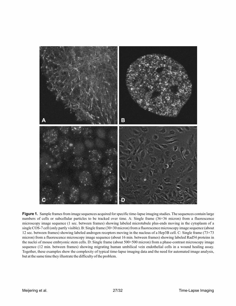
Meijering et al. 27/32 Time-Lapse Imaging
A B
C D
Figure 1. Sample frames from image sequences acquired for specific time-lapse imaging studies. The sequences contain large numbers of cells or subcellular particles to be tracked over time. A: Single frame (36×36 micron) from a fluorescence microscopy image sequence (1 sec. between frames) showing labeled microtubule plus-ends moving in the cytoplasm of a single COS-7 cell (only partly visible). B: Single frame (30×30 micron) from a fluorescence microscopy image sequence (about 12 sec. between frames) showing labeled androgen receptors moving in the nucleus of a Hep3B cell. C: Single frame (73×73 micron) from a fluorescence microscopy image sequence (about 16 min. between frames) showing labeled Rad54 proteins in the nuclei of mouse embryonic stem cells. D: Single frame (about 500×500 micron) from a phase-contrast microscopy image sequence (12 min. between frames) showing migrating human umbilical vein endothelial cells in a wound healing assay. Together, these examples show the complexity of typical time-lapse imaging data and the need for automated image analysis, but at the same time they illustrate the difficulty of the problem.

Meijering et al. 28/32 Time-Lapse Imaging
IMAGE ACQUISITION
Microscope Setup
Spatial Dimensionality
Temporal Resolution
IMAGE PREPROCESSING
Image Denoising
Image Deconvolution
Image Registration
TRAJECTORY ANALYSIS
Geometry Measurements
Diffusivity Measurements
Velocity Measurements
IMAGE ANALYSIS
Cell Tracking Cell Segmentation
Cell Association
Particle Tracking Particle Detection
Particle Association
Time-LapseMicroscopy
Imaging
Figure 2. The circle of life in time-lapse microscopy imaging. The diagram depicts the successive steps in the imaging process and, at the same time, gives an overview of the topics addressed in this chapter. Following image acquisition, preprocessing is often required to increase the success of subsequent automated analysis of the images and, eventually, of the resulting trajectories. The circular structure of the diagram reflects the iterative nature of the imaging process: the results of previous experiments usually trigger the planning of new experiments.

Meijering et al. 29/32 Time-Lapse Imaging
5D
xy
z
s
t
4D
xy
s
t
xy
z
t
3D
xy
t
x
s
t
2D
x
t
1D
t
t
y
z
t
Figure 3. Possible image configurations and dimensionalities in time-lapse microscopy imaging. Each dimension corre-sponds to an independent physical parameter or coordinate: x and y commonly denote the in-plane spatial coordinates, z the depth or axial coordinate, t the time coordinate, and here s denotes any spectral parameter, such as wavelength. Notice that dimensionality, as used above, does not necessarily describe the image configuration unambiguously. For example, 4D imaging may refer to spatially 2D multispectral time-lapse imaging, or to spatially 3D time-lapse imaging. To avoid confusion, it is better to use the abbreviations 2D and 3D for referring to spatial dimensionality only, and to indicate explicitly whether the data also involves a temporal or spectral coordinate. Therefore, in this chapter, we indicate spatially 2D and 3D time-lapse imaging by 2D+t and 3D+t, respectively, rather than by 3D and 4D.

Figure 4. Different types of diffusivity characterized by the MSD as a function of time lag. The idealized curves apply to the case of noise-free measurements and consistent object motion. In the case of localization errors and non-consistent motion, the curves will show offsets and irregularities.
MS
D
time
normal
flow
impeded
confined
Meijering et al. 30/32 Time-Lapse Imaging

D
t = 0 t = 4
t = 8 t = 12
E
A B C
Figure 5. Sample results from applying the described level-set based cell tracking algorithm. A-C: Segmentations (white contours) for arbitrary frames taken from three different 2D+t image sequences. The examples illustrate the ability of the algorithm to yield plausible contours even in the presence of considerable object noise and strongly varying intensities, as caused, for example, by photobleaching in the case of FRAP experiments. D: Visualization of segmented surfaces of cell nuclei in four frames of a 3D+t image sequence. The renderings demonstrate the ability of the algorithm to keep track of cell division. E: Illustration of tracking cell division in a 2D+t image sequence.
Meijering et al. 31/32 Time-Lapse Imaging

A B
C
tim
e
D
Figure 6. Sample results from applying the described SMC-based particle tracking algorithm. A and B: Estimated current locations (white squares) and trajectories (white curves) up to the current time, for the most prominent particles in an arbitrary frame from the 2D+t image sequences shown in Figure 1A and 1B, respectively. The trajectories in B are due to Brownian motion and are therefore strongly confined. C: Artistic rendering of the trajectories linking multiple frames of data set A. D: Illustration of the capability of the algorithm to deal with photobleaching, to capture newly appearing particles, detect particle disappearance, and handle closely passing particles.
Meijering et al. 32/32 Time-Lapse Imaging