Noname manuscript No.(will be inserted by the editor)

Time-focused clustering of trajectories of moving objects

Mirco Nanni · Dino Pedreschi

the date of receipt and acceptance should be inserted later

Abstract Spatio-temporal, geo-referenced datasets are growing rapidly, and will be more inthe near future, due to both technological and social/commercial reasons. From the data min-ing viewpoint, spatio-temporal trajectory data introduce new dimensions and, correspond-ingly, novel issues in performing the analysis tasks. In this paper, we consider the clusteringproblem applied to the trajectory data domain. In particular, we propose an adaptation of adensity-based clustering algorithm to trajectory data based on a simple notion of distancebetween trajectories. Then, a set of experiments on synthesized data is performed in orderto test the algorithm and to compare it with other standard clustering approaches. Finally, anew approach to the trajectory clustering problem, calledtemporal focussing, is sketched,having the aim of exploiting the intrinsic semantics of the temporal dimension to improvethe quality of trajectory clustering.

Note: The authors are members of the Pisa KDD Laboratory, a joint research initiative ofISTI-CNR and the University of Pisa:http://www-kdd.isti.cnr.it .

1 Introduction

Spatio-temporal, geo-referenced datasets are growing rapidly, and will be more in the nearfuture. This phenomenon is due to the daily collection of transaction data through databasesystems, network traffic controllers, web servers, sensor networks. In prospect, an impor-tant source is telecommunication data from mobile phones and other location-aware devices– data that arise from the necessity of tracking such wireless, portable devices in order tosupport their interaction with the network infrastructure. But other than ordinary commu-nication operations, the large availability of these forms of geo-referenced information isexpected to enable novel classes of applications, where the discovery of knowledge is the

Mirco NanniISTI - Institute of CNR, Via Moruzzi 1 – Loc. S. Cataldo, 56124 PisaPhone: +39 050 3152934, Fax: +39 050 3138091E-mail: mirco.nanni@isti.cnr.it

Dino PedreschiDipartimento di Informatica, Universita di Pisa, Via F. Buonarroti 2, 56127 Pisa, ItalyPhone: +39 050 2212752, Fax: +39 050 2212726E-mail: pedre@di.unipi.it

2

key step. As a distinguishing example, the presence of a large number of location-aware,wireless mobile devices presents a growing possibility to access their tracking logs and re-construct space-time trajectories of these personal devices and their human companions: tra-jectories are indeed the traces of moving objects and individuals. These mobile trajectoriescontain detailed information about personal and vehicular mobile behaviour, and thereforeoffer interesting practical opportunities to find behavioural patterns, to be used for instancein traffic and sustainable mobility management.

However, spatio-temporal data mining is still in its infancy, and even the most basicquestions in this field are still largely unanswered: what kinds of patterns can be extractedfrom trajectories? Which methods and algorithms should be applied to extract them? Onebasic data mining method that could be applied to trajectories isclustering, i.e., the discoveryof groups ofsimilar trajectories.

Spatio-temporal trajectory data introduce new dimensions and, correspondingly, novelissues in performing the clustering task. Clustering moving object trajectories, for example,requires finding out both a proper spatial granularity level and significant temporal sub-domains. Moreover, it is not obvious to identify the most promising approach to the clus-tering task among the many in the literature of data mining and statistics research; neitherit is obvious to choose among the various options to represent a trajectory of a moving ob-jects and to formalize the notion of (dis)similarity (or distance) among trajectories. A briefaccount of the research in this area is reported in Section 2.

In this context, we precisely address the problem of trajectory clustering. Our basic as-sumption on source data is that a collection of individual trajectories of moving objects canbe reconstructed in an approximated way on the basis of tracking log data left by the objectsas they move within the network infrastructure. As an example, a mobile phone that movesamong the various cells of the wireless network leaves, during its interactions with the net-work, a set of triples(id, loc, t), each specifying the localization at spaceloc and at timetof the phoneid. Starting from the set of triples for a given objectid is therefore possible, inprinciple, to approximate a functionfid : time→ space, which assigns a location to objectid for each moment in a given time interval. We call such a function atrajectory, and weconcentrate on the problem of clustering a given set of trajectories. This basic assumptionis consistent with the form of tracking log data that are (or can be) collected in the wire-less network infrastructure; for the sake of concreteness, we could count in our research onthe availability of a synthesizer of trajectory data, which has been developed at our labora-tory (Giannotti, Mazzoni, Puntoni & Renso 2005) and has been used to create the sourcetrajectory datasets employed in the empirical evaluation of the achieved results.

We address two distinct questions: (i) what is the most adequate clustering method fortrajectories, and (ii) how can we exploit the intrinsic semantics of the temporal dimensionto improve the quality of trajectory clustering.

Concerning the first problem, we advocate thatdensity-based clustering, in the formsoriginally proposed in (Ester et al. 1996) and (Ankerst, Breunig, Kriegel & Sander 1999), isparticularly well-suited to the purpose of trajectory clustering, given its distinctive features:

– the ability to construct non-spherical clusters of arbitrary shape, unlike the classicalk-means and hierarchical methods,

– the robustness with respect to noise in the data,– the ability of discovering an arbitrary number of clusters to better fit the source data

– like hierarchical methods, but with a considerably lower complexity (O(nlogn) vs.O(n2)).

3

All the above are key issues for trajectories: it is likely that trajectories of cars in theurban traffic tend to agglomerate in snake-like, non-convex clusters, that many outlier tra-jectories should not be included in meaningful clusters but rather considered as noise, andthat the number of clusters is unpredictable. Density-based clustering algorithms deal withthe above problems by agglomerating objects within clusters on the basis ofdensity, i.e.,the amount of population within a given region in the space. In our approach, we gener-alize the spatial notion of distance between objects to a spatio-temporal notion of distancebetween trajectories, and we thus obtain a natural extension of the density-based cluster-ing technique to trajectories. To analyze the consequences of our approach, we consider aparticular density-based clustering algorithm, OPTICS (Ankerst et al. 1999), and proposean empirical comparison with several traditionalk-means and hierarchical algorithms; weshow how, on a set of experiments, our density-based approach succeeds in finding the nat-ural clusters that are present in the source data, while all the other methods either fail orobtain less accurate results. To some extent, this sort of empirical evidence points out thatdensity-based trajectory clustering yields a better quality output, with respect to the othertraditional methods.

The second contribution of this paper istemporal focusing. Here, we stress that the tem-poral dimension plays a key role in trajectory clustering: two trajectories, which are verydifferent considering the whole time interval of their duration, may become very similarif restricted considering a smaller sub-interval – an obvious observation with reference to,e.g., the vehicle trajectories in the urban traffic. It is therefore interesting to generalize tra-jectory clustering with a focus on the temporal dimension – basically enlarging the searchspace of interesting clusters by considering the restrictions of the source trajectories ontosub-intervals of time. Our proposed algorithm for temporal focussing is therefore aimed atsearching the most meaningful time intervals, which allow to isolate the (density-based)clusters of higher quality.

The plan of the paper follows. In the next Section we briefly discuss related work, whilein Section 3 we define trajectories and their distances. In Section 4 we revise density-basedclustering and the OPTICS algorithm, while in Section 5 we propose the extension of OP-TICS to trajectories and empirically evaluate our proposal. In Section 6 we propose thetemporal focusing methods, together with some preliminary empirical experiments. Finally,in Section 7 we report the results of a larger experimentation aimed at assessing both theoutput quality and the performances of the proposed algorithm.

2 Related Work

In recent years, the problem of clustering spatio-temporal data received the attention ofseveral researchers. Most of the actual work is focused on two kinds of spatio-temporal data:moving objects trajectories (the topic of this paper), such as traffic data, and geographicallyreferenced events, such as epidemiological and geophysical data collected along severalyears.

Trajectory clustering. In one of the first works related to the topic, Ketterlin (Ketterlin1997) considers generic sequences (thus modelling trajectories as sequences of points) to-gether with a conceptual hierarchy over the sequence elements, used to compute both thecluster representatives and the distance between two sequences. Nanni, one of the authorsof the present paper adapted two classical distance-based clustering methods (k-means andhierarchical agglomerative clustering) to trajectories (Nanni 2002). In the first part of thepresent work, we perform a step in the same direction, by adapting instead the density-based

4

approach to trajectories. An alternative strategy is to apply to trajectories some multidimen-sional scaling technique for non-vectorial data, e.g., Fastmap (Faloutsos & Lin 1995), whichmaps a given data space to an Euclidean space preserving (approximatively) the distancesbetween objects, so that any standard clustering algorithm for vectorial data can be applied.Other distances can be inherited from the time-series domain, with the implicit assump-tion that the temporal component of data can be safely ignored and replaced by an order inthe collected data values: the most common distance is the Euclidean metric, where eachvalue of the series becomes a coordinate of a fixed-size vector; other approaches, which tryto solve problems such as noise and time warping, include the computation of the longestcommon subsequence of two series (e.g., see (Vlachos, Gunopulos & Kollios 2002)), thecount of common subsequences of length two (Agrawal, Lin, Sawhney & Shim 1995), thedomain-dependent extraction of a single representative value for the whole series (Kalpakis,Gada & Puttagunta 2001), and so on. The main drawback of this transformational approachis ad-hoc nature, bound to specific applications. A thoroughly different method, proposedby Gaffney and Smyth (Gaffney & Smyth 1999), is model-based clustering for continuoustrajectories, which groups together objects which are likely to be generated from a commoncore trajectory by adding Gaussian noise. In a successive work (Chudova, Gaffney, Mjol-sness & Smyth 2003) spatial and (discrete) temporal shifting of trajectories within clustersis also considered.

Spatio-temporal density. The problem of finding densely populated regions in space-time is conceptually closely related to clustering, and it has been undertaken along severaldifferent directions. In (Hadjieleftheriou, Kollios, Gunopulos & Tsotras 2003), a system isproposed to support density queries over a database of uniform speed rectilinear trajecto-ries, able to efficiently discover the spatial locations where moving objects are – or will be– dense. In (Gudmundsson, van Kreveld & Speckmann 2004) the computational complexityand approximation strategies for a few motion patterns are studied. In particular, the authorsstudyflock patterns, that are defined as groups of at leastn moving objects (n being a param-eter) such that there exists a time interval of width larger than a given threshold where allsuch objects always lay inside a circle of given radius. A much similar objective is pursuedin (Hwang, Liu, Chiu & Lim 2005), with an emphasis on efficiency issues. Finally, in (Li,Han & Yang 2004) an extension ofmicro-clusteringto moving objects is proposed, whichgroups together rectilinear segments of trajectories that lay within a rectangle of given sizein some time interval. The objectives of such work, however, are a bit different, being fo-cused on the efficient computation of static clusters at variable time instants. The secondcontribution of this paper works in a direction similar to micro-clusters discovery. However,in addition to the more general concept of density adopted, in this paper we focus on theglobal clustering structure of the whole dataset, and not on small groups of objects.

Event clustering. A different view of the spatio-temporal clustering problem consistsin considering spatially and temporally referenced events, instead of moving objects. In thiscase, the most basic approach consists in the application of spatial clustering algorithmswhere time becomes an additional spatial dimension. In addition to that, in literature differ-ent approaches have been proposed, mostly driven by specific application domains. Amongthem, we mention Kuldorff’s spatial scan (Kulldorff 1997), a well known statistical methoddeveloped for epidemiological data which searches spatio-temporal cylinders (i.e., spatialcircular shapes which remain still for some time interval) where the rate of disease cases ishigher than outside the cylinder, and extensions for considering more flexible square pyra-mid shapes (Iyengar 2004).

5

3 A data model and distance for trajectories

In this paper we consider databases composed by a finite set of spatio-temporal objects.From an abstract point of view, a spatio-temporal objecto is represented by atrajectoryτo,i.e., a continuous function of time which, given a time instantt, returns the position at timet of the object in ad-dimensional space (typicallyd ∈ {2,3}). Formally:τo : R+ → Rd.

In a real-world application, however, trajectories of objects are given by means of a finiteset of observations, i.e. a finite subset of points taken from the real continuous trajectory.Moreover, it is reasonable to expect that observations are taken at irregular rates within eachobject, and that there is not any temporal alignment between the observations of differentobjects. This calls for an approximate reconstruction of the original trajectory. In this paper,we employ the model used in (Saltenis, Jensen, Leutenegger & Lopez 2000), where theobjects are assumed to move in a piecewise linear manner. Namely, an object moves along astraight line with some constant speed till it changes the direction and/or speed. Such modelessentially corresponds to the well known parametric 2-spaghetti approach (Chomicki &Revesz 1999).

In this work, we are interested in distances that describe the similarity of trajectories ofobjects along time and therefore are computed by analyzing the way the distance betweenthe objects varies. More precisely, we restrict to consider only pairs ofcontemporaryin-stantiations of objects, i.e., for each time instant we compare the positions of the objects atthat moment, thus aggregating the set of distance values obtained this way. This implies,in particular, that we exclude subsequence matching and other similar operations usuallyadopted in the time series field, as well as solutions that try to align – in time and/or in space– shifted trajectories.

The distance between trajectories adopted in this paper is computed in a most naturalway, as the average distance between objects, that is to say:

D(τ1,τ2)|T =R

T d(τ1(t),τ2(t))dt|T| ,

whered() is the Euclidean distance overR 2, T is the temporal interval over which trajec-toriesτ1 andτ2 exist, andτi(t) (i ∈ {1,2}) is the position of objectτi at timet. We noticethat such a definition requires a temporal domain common to all objects, which, in general,is not a hard requirement. From a conceptual viewpoint, moreover, in order to computeD()we need to compute the infinite set of distances for eacht ∈ T (e.g., in and, afterward, to ag-gregate them. However, due to the (piece-wise) linearity of our trajectories, it can be shown(Nanni 2002) thatD() can be computed as a finite sum by means ofO(n1 + n2) Euclideandistances,n1 andn2 being the number of observations respectively available forτ1 andτ2.Moreover, such distance is a metric, thus allowing the use of several indexing techniquesthat help to improve performances in several applications, including clustering.

4 Density-based clustering and OPTICS

In this section we briefly review the principles of density-based clustering, summarizing themotivations which led us to adopt this approach for trajectories, and describe the OPTICSalgorithm.

6

4.1 Density-based Clustering

The key idea of density-based clustering algorithms is that for each object in some clusterthe neighborhood of a given radiusε has to contain at least a minimum numbernpts ofobjects, i.e., the cardinality of the neighborhood has to exceed a given threshold. For thatreason, such algorithms are naturally robust to problems such as noise and outliers, sincethey usually do not significantly affect the overall density distribution of data. This is animportant feature for several real world applications, such as all those that work with datasources having some underlying random (unpredictable) component – e.g., data obtainedby observing human behaviour – or that collect data by means of not-completely reliablemethods – e.g., low-resolution sensors, sampled measures, etc. Trajectory data usually sufferof both the mentioned problems, so noise tolerance is a major requisite.

Moreover, in typical applications dealing with moving objects, such as traffic analysisor the study of PDAs usage and mobility, any strict constraint to the shape of clusters wouldbe a strong limitation, sok-means and other spherical-shape clustering algorithms could notbe generally applied (e.g., large groups of cars moving along the same road would form a”snake”-shaped cluster, not a spherical one).

The algorithms in the DBSCAN family (Ester et al. 1996) appear to be a good candidatechoice for density-based clustering, since they satisfy the above mentioned requirementsand, additionally, can be easily applied also to complex data at reasonable computationalcosts. In particular, in this paper we will focus on the OPTICS algorithm (Ankerst et al.1999), a widely known evolution of the basic DBSCAN that solves many of its technicalissues, first of all the sensitivity to input parameters. Moreover, it is worth noting that theoutput of OPTICS, thereachability plot, described in the following, is an intuitive, data-independent visualization of the cluster structure of data, that yields valuable informationfor a better comprehension of the data and that is (also) used to assign each object to itscorresponding cluster or to noise, respectively.

4.2 OPTICS

In the following, we will shortly introduce the definitions underlying OPTICS, i.e.,coreobjectsand thereachability-distanceof an objectp w.r.t. a predecessor objecto, and brieflydescribe how the algorithm works by means of a small example.

An objectp is called acore objectif the neighborhood around it is a dense region, andthereforep should definitely belong to some cluster and not to the noise. More formally:

Definition 1 (Core object) Let p∈ D be an object in datasetD, ε a distance threshold andNε(p) the ε-neighborhood ofp, i.e., the set of points{x ∈ D|d(p,x) ≤ ε}. Then, given aparameternpts∈N , p is acore objectif: |Nε(p)| ≥ npts.

Based on core objects, we have the following:

Definition 2 (Reachability-distance)Let p∈ D be an object,o∈ D a core object,ε a dis-tance threshold andNε(o) theε-neighborhood ofo. Denoting withn-distance(p) the distancefrom p to its n-th neighbor in order of proximity (n∈N ), and given a parameternpts∈N ,thereachability-distance ofp with respect too is defined as

reach−dε,npts(p,o) = max{ npts−distance(o) , d(o, p) }

7

18

0

12

3

4

5 6

78

9

1011

12

13

14

15

16

17

Y a

xis

X axis

0.02

0.04

0.06

0.08

0.1

0.12

0.14

0.16

0.18

0.2

0.22

0 1 2 3 4 5 6 7 8 9 10 11 12 13 14 15 16 17 18

Fig. 1 Sample run of OPTICS with the resulting reachability plot

The reachability-distance ofp w.r.t. o is essentially their distance, excepted whenp istoo close, in which case such distance isnormalizedto a suitable value. OPTICS works asfollows: initially a random objectp0 is chosen; then, at each iterationi, the next objectpi

chosen fromD is that with the smallest reachability-distance w.r.t. all the already visitedcore objects; the process is repeated until all objects inD have been considered.

The whole process is summarized by means of areachability plot: on the horizontal axisare represented the objects in their visit ordering0, . . . , |D|−1, and on the vertical axis, foreachi the reachability-distance corresponding topi is plotted. The sequence〈p0, . . . , p|D|−1〉is also called acluster-reorderingof the objects inD.

Intuitively, the reachability-distance of a pointpi corresponds to the minimum distancefrom the set of its predecessorsp j ,0≤ j < i. As a consequence, a high value of reachability-distance approximatively means a high distance from all other objects, and therefore indi-cates ararefiedarea. Then, clusters, i.e., dense areas, are represented as valleys in the reach-ability plot. In particular, only core objects are considered among the predecessors, whichresults in not considering noise in the creation of clusters. Figure 1 shows a sample exe-cution of OPTICS on a toy dataset with two clusters, and the corresponding values on thereachability plot. We observe that the jump from point 9 to point 10, belonging to differentclusters, corresponds to a peak in the reachability plot.

From the reachability plot we can easily obtain a partitioning of the data into a set ofclusters, plus noise: we simply need to choose a threshold to separate clusters, expressedin terms of the maximum value of the reachability distance allowed within clusters. Suchvalue, denotedε′ and set by the user, is used to separate the objects into peaks and valleys:the former will be considered noise, the latter as clustered objects. In the example in Figure1, settingε′ = 0.1, we would obtain two clusters: objects 1-9 and 11-18.

5 Extending OPTICS to trajectories

In order to define similarity measures for OPTICS over complex domains, its inventors pro-posed and tested a few solutions, classified into two classes: feature-based models and directgeometric models (Kriegel, Brecheisen, Kroger, Pfeifle & Schubert 2003). In the first case,the basic idea is to use a feature extraction function that maps the objects onto vectors inan appropriate multidimensional feature space. The similarity of two objects is then definedas their proximity in the feature space, and the closer their feature vectors are located, themore similar the objects are considered. In the second class of models, the distance is de-fined by directly using the geometry of objects. Examples include the computation of the

8

volume of the geometric intersection of the compared objects. In this paper, we followedan approach similar to the latter, since trajectories are compared and clustered by means ofthe spatio-temporal distance described in Section 3. In particular, our prototypes (both theTrajectory-OPTICS described in this section and the TF-OPTICS introduced in Section 6)have been implemented by integrating M-tree (Ciaccia, Patella & Zezula 1997), a indexfor generic metric spaces aimed at supporting efficient range queries, which are the coreoperation of the OPTICS algorithm. The results obtained in terms of performances will bediscussed in detail in Section 7. However, it is less obvious to verify that OPTICS deliverhigh quality trajectory clusters. In the next section, we provide some very intuitive and pre-liminary evidence that OPTICS finds dense and well defined trajectory clusters, with a goodtolerance to noise and outliers. A larger experimental assessment will presented later in thepaper, in Section 7.

5.1 OPTICS vs. Hierarchical and K-means algorithms

We considered a synthetic test dataset randomly generated with the C4C trajectory generator– described in Section 7.1 – composed of 250 trajectories organized into four natural clustersplus noise. The dataset is depicted in Figure 2(a), where horizontal coordinates representspatial positions and the vertical one represents time. Each cluster contains objects thatmove towards some defined direction. The objective of these experiments is to evaluatethe behaviour of OPTICS on the trajectory data domain, as compared to other classical,general purpose clustering algorithms. We applied to the dataset thek-means algorithm anda standard hierarchical agglomerative algorithm in three versions: single-linkage, complete-linkage and average-linkage. The same dataset was processed by the trajectory version ofOPTICS. All algorithms were configured to find four clusters (i.e., the expected numberof natural clusters in the data). For the output of each algorithm, the averagepurity of theclusters (i.e., percentage of objects in the cluster that belonged to the corresponding realcluster) and the average of theircoverage(i.e., percentage of objects of the real cluster thatappear in the cluster found). The results are discussed below:

– K-means yields a100%coverage but only a53.7% purity. That is due to the fact thatit merges together two clearly distinguished clusters, since it is sensible to noise andoutliers. In fact, a whole resulting cluster is composed only of noisy objects.

– The hierarchical single-linkage algorithm yields a100% coverage but only a52.0%purity. Indeed, it is very sensitive to the chaining effect – i.e., the fact of collapsing farclusters due to a thin, yet continuous, line of objects linking them – and therefore itmerges two dense and well separated clusters because of noise and the closeness of theirborders.

– The complete-linkage algorithm yields a99%coverage but only a50.0%purity: it tendsto form clusters with equal diameter, and so, due to the presence of noise that biasessuch size, two of the natural clusters are again merged together.

– The average-linkage algorithm yields a100%coverage but only a50.5%purity: it keepsclusters with balanced average intra-cluster distance, which usually results in a behaviorsimilar to the complete-linkage case. Again, a pair of natural clusters is merged.

– Finally, Trajectory-OPTICS yields a93.5% coverage and also a99.0% purity, i.e., thebest trade-off between the two measures. As we can see from the resulting reachabilityplot (Figure 2(b)), Trajectory-OPTICS correctly finds the four natural clusters, whichcan be easily isolated by selecting a proper value for theε parameter (ε = 24 in ourexample, but any value that crosses the three central protrusions yield the same result).

9

Time

X axis

Y axis

Time

(a) Input dataset

15

20

25

30

35

40

45

50

55

60

0 50 100 150 200 250

Rea

chab

ility

-dis

tanc

e

OPTICS Objects order

Reachability plot

Epsilon = 24

(b) OPTICS Reach. plot

Fig. 2 A synthesized dataset (a) and the corresponding reachibility plot for OPTICS

6 Temporal Focusing

The approach to trajectory clustering presented above treats trajectories as unique, indivisi-ble elements, and tries to group together those moving objects that globally move in a similarway, ”smoothing” the effect of any sporadic divergence in their movement. However, suchglobal trajectory clustering may sometime be misleading and yield counter-intuitive results.In particular, it might keep separated objects that moved together for a significant amount oftime, while gathering objects that constantly keep a significant distance between them.

From real world experience, we learnt that not all time intervals have the same impor-tance. A meaningful example is urban traffic: in rush hours a large quantity of people movefrom home to work and viceversa, or, more generally, from/to largely shared targets. There-fore, we can expect that the sheer size of the population sample will make it possible forgroups of individuals having similar destinations to clearly emerge from traffic data to formcompact clusters. In quiet periods of the day, on the contrary, we expect to mainly observestatic individuals, whose distribution on the territory is more driven by the geographical pop-ulation density than by collective motion behaviors. This is a general problem not limited tourban traffic, and, while in this sample context some interesting hours of the day for clusteranalysis can be guessed – e.g., typical morning rush hours –, in other, less understood casesand domains it might be not possible to fix a priori criteria for choosing the right periodof time. In these cases, some automatic mechanism to discover the most interesting inter-vals of time should be applied. In what follows we formalize the problem mentioned above,and suggest a solution. We anticipate that we will consider only single intervals of time inour search problem, thus not taking into account more complex patterns of time, such asperiodical patterns or irregular sets of disjoint time intervals.

6.1 Problem setting

As discussed above, there may exist time segments where the clustering structure of ourmoving objects dataset is clearer than just considering the whole trajectories. In order todiscover such clustering structure, then, we should provide a method for locating the righttime interval, and focus the clustering process on the segments of trajectories that lay in thatinterval, ignoring the remaining parts.

10

Our general approach consists in the following: the Trajectory-OPTICS algorithm ismodified to compute distances between trajectories focusing on any time interval specifiedby the user; therefore, we (hypothetically) apply such algorithm to each possible time in-terval, evaluate each result obtained and determine the best one. This entails solving thefollowing optimization problem:

argmaxθ

Q (D,θ)

whereD is the input dataset andQ is a quality function that measures the goodness ofthe clustering results obtained with the parametersθ. The set of parametersθ can contain,in a general setting, several different components, e.g.: basic parameters for OPTICS, atemporal window, a spatial granularity, etc. In this work we will focus on time windows,so θ = 〈 ε,ε′,npts, I 〉, ε, ε′ and npts being the already mentioned general parameters forOPTICS andI being the time window we are focusing on. Moreover, since OPTICS isnot very sensible to its input parametersnpts andε, we can assume that they are set beforeapproaching the optimization problem, so that the only variables of the problem remainIandε′.

We observe that the problem introduced above can be seen as a subspace clustering prob-lem. In particular, if we assume that time is discrete, and therefore the time intervalI can bereduced to a finite sequence ofN time points, trajectories can be seen as2N-dimensional ob-jects, and our objective is to discover2N′ contiguous dimensions (N′ ≤N) that optimize ourquality function. However, in all works of the subspace clustering literature, the dimensionsare not related to each other by any specific semantics, differently from the temporal seman-tics that underlies trajectories. In particular, distances that are additive w.r.t. dimensions1 areusually applied, making density of regions a monotonic function w.r.t. the dimensions (i.e.,dense regions on someN-dimensional space always correspond to dense regions on any ofits N−1-dimensional subspaces). On the contrary, when dealing with trajectories we haveto deal with a semantics of time, that significantly modifies the problem. The most directand relevant effects are the following: (i) a notion of contiguity is defined, that has to bepreserved when selecting subspaces; and (ii) a distance between objects is given, that is notadditive w.r.t. dimensions. As a consequence, actual subspace clustering techniques are notapplicable in our case. In what follows, we propose an heuristic solution to this new variantof the subspace clustering problem.

6.2 Quality measure

The first issue to solve, now, is the definition of a quality functionQ , which can provide agood criterion for deciding whether a clustering result is better than another. Any suitabledefinition should take into account the nature of clusters we obtain. In particular, since we areworking with density-based tools, typical dispersion measures cannot be applied, becausewe can have good non-spherical clusters, which, in general, are not compact.

In the density-based setting, the standardhigh intra-cluster vs. low inter-cluster similar-ity principle could be naturally translated into ahigh-density clusters vs. low-density noiserule. Highly dense clusters can be considered interesting per se, while having a rarefiednoise means that clusters are clearly separated. Put together, these two qualities seem toreasonably qualify agood(density-based) clustering result.

1 I.e., distances betweenN-dimensional objects can be written as a sum ofN contributions independentlycomputed on each dimension. E.g., it holds for Euclidean distances, sinced2(a,b) = ∑N

i=1(ai −b1)2.

11

The reachability plot returned by the OPTICS algorithm contains a summary of theinformation on data density we need. Therefore, we can simplify the computation of theQmeasure by deriving it from the corresponding reachability plot, since density at each pointcan be estimated by the corresponding reachability-distance.

Definition 3 Let D be an input dataset of trajectories,I a time interval andε′ a densitythreshold parameter. Then, theaverage reachability, R(D, I ,ε′), is defined as the averagereachability-distance of non-noise objects:R(D, I ,ε′) = avg{r|〈p0, . . . , p|D|−1〉 is OPTICScluster reordering∧ r = reach−dε,npts(pi)∧ r ≤ ε′}. When clear from the context, averagereachability will be denoted asRC (reachability of clustered objects). When noε′-cut isspecified (i.e.,ε′ = ∞), average reachability will also be denoted asRG (global reachability).

In this work, in particular, we will give the greatest importance to high-density clusters,which seem to be the most essential property between the two listed above, and will not takeinto consideration noise. For the latter, we will consider as sufficient the minimum densityrequirement specified by the user through theε′ parameter – noise, by definition, cannotbe denser than such threshold. As mentioned above, density within clusters can be easilyestimated by means of in-cluster reachabilities, leading to the following simple formulation:

Definition 4 Let D be an input dataset of trajectories,I a time interval andε′ a densitythreshold parameter. Then, we define theQ 1 quality measure as follows:

Q 1(D, I ,ε′) =−R(D, I ,ε′).

Dispersed clusters yield high reachability distances, and therefore highly negative valuesof Q 1, while compact clusters yield values ofQ 1 closer to zero. Moreover, notice thatQ 1,being an average value and not a simple sum, does not force any preference for small orlarge clusters.

6.3 Self-tuning of parameters

The search for an optimal time interval requires to iteratively analyze different views ofthe input trajectory dataset. However, each view can result in a quite different reachabilityplot, with peaks and valleys of highly variable size. As a consequence, it is not possible todetermine a single value of theε′ that is valid for all time intervals. Since it is not reasonableto ask the user to choose a suitable value for each interval analyzed, we should design anautomated method for the purpose. We describe a solution to the problem that requires theuser to specify an initialε′0 value for the largest time interval, and then automatically adaptssuch value to the smaller intervals.

In general, the optimalε′ value for an intervalI depends on several variables. We con-sider a simple solution and assume that densities follow some general trend, so that a globalrescaling factor for density values can be computed. Such rescaling can be applied toε′0 toobtain the actualε′. The overall density for a given time interval can be estimated in severalways, the simplest being the average reachability-distanceRG. Adopting such measure anda linear rescaling, we have the following value forε′:

ε′(D, I ,ε′0) =RG

R0G

ε′0

whereR0G denotes the value ofRG on the largest time interval. In order to test the re-

liability of the ε′ re-scaling method proposed above, we performed an experiment on the

12

0

10

20

30

40

50

60

Rea

chab

ility

Objects reordering

Reachability plot for I=[0,100]

"Reasonable" ε values Chosen ε value

0

10

20

30

40

50

60

Rea

chab

ility

Objects reordering

Reachability plot for I=[20,60]

Adjusted ε values Adjusted chosen ε value

Fig. 3 Example ofε adaptation fromI = [0,100] to I = [20,60]

trajectory dataset considered in Section 5.1. We assumed that for each reachability plot it ispossible to define an interval for the acceptable values of theε′ parameter, and that the spe-cific ε′ value that a generic user would choose follows a random uniform distribution overthe above mentioned interval. Figure 3 (left) depicts an example of reasonable values overthe largest time interval (0−100), represented by a dark band, with an example of chosenvalue forε. The same Figure (right) shows also their mapping to a smaller interval (20−60).

In our experiment, We considered 50 samples that include time intervals of all sizes andof variable position, i.e., not biased towards initial or final intervals. Then, for each timeinterval I considered, we compute the probability that a value chosen on the0−100 timeinterval isadjustedto a reasonable value onI , i.e., a value that lays within correspondinginterval of reasonable values. Then, we compute the average probability of success, over allcases. The result is the following: given a random intervalI and anε value randomly chosenon the reachability plot of the0− 100 time interval, in the 80.5% of the cases suchε ismapped onI to a reasonable value. Such estimate shows that, in spite of its simplicity, theproposed rescaling method is empirically reliable.

6.4 Evaluating and improvingQ 1

In order to acceptQ 1 as a suitable quality measure, an important property to verify is itsnon-shrinkingbehavior w.r.t. interval size, i.e., the fact that not all time intervalsI contain atleast a subintervalI ′ having a higher quality measure. Formally, we would like to refute thefollowing property:∀I .∃I ′ ⊂ I : Q 1(I ′) > Q 1(I). In fact, such property would imply that theoptimal time interval forQ 1 is always a minimal-size interval, thus trivializing the problemand yielding uninteresting results. Fortunately, it is easy to find a counterexample:

Example 1Let consider a set of trajectories over a time interval that is formed by exactlytwo time units: in the first unit trajectories are very dense, while in the second one they be-come more rarefied, although not beyond the given density threshold. Now add a trajectorythat is always distant from all the others, but in the first time interval is close enough to themto be part of the same cluster, while in the second one immediately gets extremely far fromthem. Then, focusing on the first interval, all trajectories belong to the same cluster but, dueto the single outlier trajectory described above, it has only a medium density. In the sec-ond interval, the outlier trajectory becomes noise, but the remaining ones are a bit rarefied,so density is not high here. On the overall interval, we get all the positive aspects of boththe sub-intervals: the outlier trajectory is considered as noise, and so the first sub-intervalyields a very high density that is able to lift the overall density beyond the limits of the twosub-intervals. As a consequence, the larger interval has a better quality than its sub-intervals.

13

Time

All complete trajectories

X axis

Y axis

Time

Quality function Q1 over all time intervals

Optimum

0

20

40

60

80

100

Tstart

0 20 40 60 80 100

Tend

-12-11-10-9-8-7-6-5-4-3-2

Q1 = -RC

Fig. 4 Sample dataset and correspondingQ1 plot

The second step in validating the quality measure is a test against a dataset. In Figure 4,on the left, a set of 320 trajectories is shown. Such dataset was generated by using the alreadymentioned C4C system, and contains (in addition to noise) three groups of trajectories thattend to move together within a central time interval, and tend to spread across a wider area inthe other intervals. Trajectories are defined over the[0,100] time interval, that is discretizedinto 50 time units of 2 seconds each. In figure 4, on the right, a plot of theQ 1 measureover all time intervals is depicted: the two horizontal axes represent the boundaries of timeintervals, so that only the lower-left part of the plane – where the lower bounds of intervalsare smaller than upper bounds – is significant. Below the 3D plot, the corresponding (plane)contour plot gives a bi-dimensional view of the same value, with the optimal interval pointedby an arrow. The plot shows that the optimum is located along the diagonal, which representsthe intervals with the smallest size. In general, there is a strong bias towards small intervals,even though we can notice the presence of several central regions in the plot – correspondingto larger intervals – withQ1 values close to the optimum.

When only very small variations ofQ1 are observed, it is reasonable to prefer largerintervals, since they are more informative. We can do that by slightly promoting larger in-tervals directly in the quality measure. A simple solution consists in adding a factor thatincreases the quality function as the interval size grows, but only very slowly, in order toavoid excessive bias. To this purpose, we adopt the following variation of theQ1 measure:

Q2(D, I ,ε′) = Q1(D, I ,ε′)/ log10(10+ |I |)In Figure 5 we can see the plot corresponding to the newQ 2 measure. As we can notice, theoptimum value (pointed by the arrow) is now in the central region, on the[30,72] interval,which means that the small correction introduced is sufficient to discover significantly largedense intervals. On the righthand plot we see the resulting clusters, where the segments ofthe clustered trajectories contained in the optimal time interval are emphasized: the densestsegments of the natural clusters present in the data are clearly discovered, leaving out theportions of trajectory where the objects start/end dispersing.

6.5 Searching strategies

The basic method for finding the time interval that maximizesQ 2 is an exhaustive searchover all possible intervals. Such approach is obviously very expensive, since it adds to thecomplexity of OPTICS a quadratic factor w.r.t. the the maximum size of time intervals,expressed in time units. More precisely, given a granularity of timeτ, the global interval

14

Quality function Q2 over all time intervals

Optimum

0

20

40

60

80

100

Tstart

0 20 40 60 80 100

Tend

-5-4.5

-4-3.5

-3-2.5

-2-1.5

-1

Q2 = - RC / log(10+|I|)

Time

All trajectories with optimal clusters

Complete trajectoriesOptimal Clusters

X axis

Y axis

Time

Fig. 5 Q2 plot on sample dataset and corresponding output clusters

I0 is divided intoNt = |I0|/τ time units. Then, the cost of an exhaustive search isO(N2t ·

OPTICS(n)) = O(N2t nlogn).

A natural alternative to the exhaustive search of a global optimum is the search of lo-cal one, adopting some greedy search paradigm. We considered a standard hill climbingapproach, where a randomly chosen solution (i.e., time interval) is iteratively modified, try-ing to improve the quality function at each step. We follow the procedure described below,whereτ is the chosen temporal granularity andI0 the largest interval:

1. Choose an initial random time intervalI ⊆ I0;2. Let I ′ = argmaxT∈NeighI Q 2(D,T,ε′), whereNeighI = {T ∈ {[Ts±τ,Te], [Ts,Te±τ]}|T ⊆

I0} andI = [Ts,Te];3. If Q 2(D, I ′,ε′) > Q 2(D, I ,ε′) then letI := I ′ and return to step 2; otherwise stop.

The total cost of the search procedure isO(niternlogn), where the number of iterationsniter has a worst-case value ofO(N2

t ), but usually assumes much smaller values, linear inNt . Executing the greedy search over our sample dataset from all possible starting points,we obtained the exact global optimum in the 70.7% of cases, which provides the successprobability when seed points in the search strategy are chosen in a uniformly random way.Therefore, on this sample data we reach a high success probability with a small number oftrials (with 5 runs we have over the 99.8% probability of finding the global optimum on thisdataset). On the average, each run required around 17 steps and 49 OPTICS invocations –corresponding to less than4% of the invocations required by the exhaustive search – thuskeeping computational costs within reasonable limits.

7 Experiments

In this section we present a set of experiments aimed at assessing efficiency and effectivenessof the Trajectory-OPTICS system (T-OPTICS) and its time-focused version (TF-OPTICS).The datasets used in experiments have been synthetically generated by the C4C algorithm,anad hocdata generator for trajectories with clusters briefly described below.

7.1 The C4C synthetic data generator

The C4C generator is a new, revised version of CENTRE (Giannotti et al. 2005). CENTREis a general purpose trajectory generator able to simulate a large variety of movements be-

15

Fig. 6 Sample C4C dataset (spatial projection)

haviors, and the generation process is driven by several user defined parameters that act onspeed, direction, agility and so on.

C4C (CENTRE for Clustering) is a generator of spatio-temporal objects that evolvein space and time producing a sequence of samples (i.e., spatial locations and their cor-responding observation times) called trajectories. The main idea is to generate trajectoriesthat follow some pre-defined clusters in order to stress and probe the limits of a clusteringalgorithm.

The core concept of C4C is to model a cluster with a sequence of rectangles (zonesof attraction) placed within the workspace of the generator: one object assigned to onecluster must reach and cross the first zone of the sequence and subsequently all the oth-ers, respecting some temporal constraints defined by the user. On one hand, the temporalconstraints definewhenan object belonging to a cluster starts to follow its correspond-ing rectangles, i.e., the typical behavior that characterizes the objects in the cluster. Onthe other hand, the density of clusters directly depends on the area of the rectangles inthe sequence: objects forced to pass through small rectangles will produce denser groupsof trajectories than others that can pass through larger rectangles. More in detail, eachcluster is defined as a set ofm sub-clusters{SubC1, . . . ,SubCm} (m > 0). A sub-clusterSubC is defined as a single step of the generation, and is characterized by four values:SubC= 〈StartPos,EndPos,StartTime,EndTime〉, whereStartPosrepresents the rectanglewhere the object starts evolving andEndPosthe one where it stops.StartTimeandEndTimedescribe the time restrictions, so that the object has to start from a point inStartPosat timeStartTimeand reach a point inEndPosat time EndTime. Finally, the sequence of sub-clusters that defines a cluster must be sorted and continuous, i.e., times between adjacentsub-clusters has to be non decreasing (EndTime(i) < StartTime(i +1), for 0< i < m) and asub-cluster has to start from the destination rectangle of the previous one (StartPos(i +1) =EndPos(i), for 0 < i < m).

Figure 6 shows a (spatial projection view of a) sample dataset generated by C4C, withthe corresponding rectangles used in the generation. Trajectories that follow a cluster haveto move from a randomly chosen point in a rectangle to another one in the destinationrectangle. As we can see in the figure, there are rectangles of different sizes that we canuse to define clusters of different densities: small rectangles will produce close trajectories,and therefore dense clusters. Moreover, a subset of trajectories do not follow any cluster,generating simple noise. In particular, the figure shows an instance of 1000 trajectories with5 clusters with slightly different densities.

The generation of trajectories and clusters is driven by two sets of input parameters.The first set contains numerical parameters with some general information like random dis-

16

Dataset n.cluster density type noise

A 5 high simple noB 5 high complex yesC 3 mixed simple noD 8 medium complex noE 4 mixed simple noF 3 mixed simple yes

Table 1 Datasets in brief

tributions settings used to control random movements of the objects, number of objects togenerate, definition of clusters (times restrictions and rectangles they have to visit), etc.The second sets of inputs provides spatial information about the rectangles used to defineclusters, i.e., their position on workspace and their size. In particular, C4C can import suchinformation through GML documents (an XML format with geographical extensions), sothese inputs can be generated by means of any GIS platform that supports it – e.g., theJUMP environment, used to generate the datasets for our experiments.

The generation process of a single spatio-temporal object takes the following steps:

– Initial positioning: the object is randomly positioned within the workspace.– Move to first sub-clusterStartPos: once the object has been placed in the workspace, the

generator assigns it to a cluster, and initializes its direction and speed in such a way thatthe object is able to reach a point of rectangleStartPosof the first sub-cluster on time(i.e., not later thanStartTime).

– Evolution of a sub-cluster: the object moves towards its current destinationEndPos, pos-sibly performing some deviations that introduce noise in process, and adjusting directionand speed along the generation in order to reach the destination rectangle in time.

– End of cluster-like movement: when the object completes all the sub-clusters it was as-signed to, it chooses a final destination (inside the workspace, again) and moves towardsit (with possible perturbation) until the generation process is stopped.

7.1.1 Datasets description

In order to test our clustering algorithms, we used C4C to generate 6 datasets containingaround 10000 trajectories, each composed of a variable number of observations, rangingfrom 10 to 30. Each dataset has different characteristics, in order to stress the algorithm bysimulating different scenarios, so for each one we chose a different number and positionsof the rectangles, different sizes and different levels of noise. Table 1 summarizes the char-acteristics of the datasets: the number of clusters, their density (high for clusters formed bysmall rectangles, and so on, while mixed stands for a mix of clusters in the same dataset hav-ing different densities), their type (simple if clusters contain only one sub-cluster, complexotherwise) and presence of noise.

7.2 Performance evaluation

7.2.1 Trajectory-OPTICS.

In order to measure the scalability of the T-OPTICS algorithm (without time-focusing) weperformed several runs of the system over input datasets of growing size. Such input data

17

0

200

400

600

800

1000

1200

1400

1600

1800

2000

1000 2000 3000 4000 5000 6000 7000 8000 9000 10000

Exe

c. T

ime

(sec

.)

N. of trajectories

Fig. 7 Average performances of T-OPTICS

has been obtained as samples of the datasets generated through the C4C system, describedin the previous section. A summary of the (average) execution times obtained is depicted inFigure 7.

As the graph shows, the curve apparently grows slightly more than linearly, which isthe expected general behavior of OPTICS over any data type having an efficient indexingsupport. However, a detailed analysis of execution times reveals that (i) the greatest part ofthe computational cost of the algorithm is always due to the computation of distances; and(ii) the number of distances required to build the M-tree index and to answer the neededrange queries apparently grows quadratically, even though with small constants (that makethe phenomenon less visible in Figure 7), i.e., the M-tree seems to be not as efficient ontrajectories with our (rather complex) distance function as it has been shown to be on dif-ferent metric spaces (Ciaccia et al. 1997). However, as it will be shown in the rest of thissection, working on time sub-intervals of trajectories makes the computational cost of thedistance function smaller, making each step of the TF-OPTICS algorithm comparativelymuch cheaper than an execution of T-OPTICS.

7.2.2 Time-focused Trajectory-OPTICS.

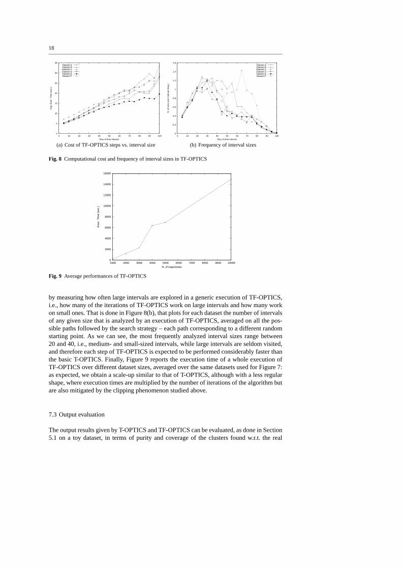
As described in Section 3, the cost of computing distances between trajectories is linearw.r.t. their complexity, i.e., the number of observations they contain. On the other hand, theTF-OPTICS algorithm essentially consists in the reiterated execution of T-OPTICS on seg-ments of trajectories, obtained by properlyclipping the original ones. The clipping processin general reduces the complexity of trajectories, and therefore the cost of computing thedistances between them. Figure 8(a) briefly reports the results of an empirical verification ofsuch a behavior, showing the relation between the (average) execution time of a single stepof TF-OPTICS (vertical axis) and the size of the time interval explored in that step (horizon-tal axis): on all datasets we obtain a linear or quasi-linear scale-up, confirming the intuitionthat, on average, the complexity of trajectories grows linearly w.r.t. their time extension. No-tice: in this and in all the following experiments, time of trajectories ranges from 0 to 100,as in the examples already considered in this paper, and in the time-focusing processes it isdiscretized into 20 segments of length 5.

Based on the results shown above, a general (though empirical) estimation of the impactthat the clipping process can produce on the execution times of TF-OPTICS can be obtained

18

0

5

10

15

20

25

30

35

0 10 20 30 40 50 60 70 80 90 100

Avg

. Exe

c. T

ime

(sec

.)

Size of time interval

Dataset ADataset BDataset CDataset DDataset EDataset F

(a) Cost of TF-OPTICS steps vs. interval size

0

0.2

0.4

0.6

0.8

1

1.2

1.4

1.6

0 10 20 30 40 50 60 70 80 90 100

N. o

f run

s ov

er in

terv

al (

Avg

.)

Size of time interval

Dataset ADataset BDataset CDataset DDataset EDataset F

(b) Frequency of interval sizes

Fig. 8 Computational cost and frequency of interval sizes in TF-OPTICS

0

2000

4000

6000

8000

10000

12000

14000

16000

1000 2000 3000 4000 5000 6000 7000 8000 9000 10000

Exe

c. T

ime

(sec

.)

N. of trajectories

Fig. 9 Average performances of TF-OPTICS

by measuring how often large intervals are explored in a generic execution of TF-OPTICS,i.e., how many of the iterations of TF-OPTICS work on large intervals and how many workon small ones. That is done in Figure 8(b), that plots for each dataset the number of intervalsof any given size that is analyzed by an execution of TF-OPTICS, averaged on all the pos-sible paths followed by the search strategy – each path corresponding to a different randomstarting point. As we can see, the most frequently analyzed interval sizes range between20 and 40, i.e., medium- and small-sized intervals, while large intervals are seldom visited,and therefore each step of TF-OPTICS is expected to be performed considerably faster thanthe basic T-OPTICS. Finally, Figure 9 reports the execution time of a whole execution ofTF-OPTICS over different dataset sizes, averaged over the same datasets used for Figure 7:as expected, we obtain a scale-up similar to that of T-OPTICS, although with a less regularshape, where execution times are multiplied by the number of iterations of the algorithm butare also mitigated by the clipping phenomenon studied above.

7.3 Output evaluation

The output results given by T-OPTICS and TF-OPTICS can be evaluated, as done in Section5.1 on a toy dataset, in terms of purity and coverage of the clusters found w.r.t. the real

19

K-means HC-avg T-OPTICS TF-OPTICSDataset purity coverage p c p c p c

A 0.798 0.8 0.761 0.74 1 0.33 1 0.449B 0.769 0.749 0.606 0.608 0.661 0.222 0.694 0.283C 0.997 0.997 1 1 1 0.365 1 0.365D 0.807 0.83 0.992 0.992 0.952 0.325 0.967 0.375E 0.626 0.626 0.624 0.743 0.878 0.23 0.992 0.397F 0.711 0.653 0.334 0.321 0.746 0.301 0.975 0.347

Table 2 Comparison of T-OPTICS and TF-OPTICS output results

Dataset P(success) OPTICS runs Q2 errorA 9.05% 5.40% 30.95%B 2.86% 4.53% 48.46%C 2.38% 4.69% 93.49%D 3.81% 4.28% 31.03%E 5.24% 5.40% 34.70%F 4.29% 4.49% 22.00%

Table 3 Results of the search heuristic

clusters in the datasets. A summary of such measures is given in Table 2, where they arecompared with analogous values obtained by applying a K-means and an average-basedhierarchical approach (HC-avg, in short).

We notice in particular that: (i) in most of the cases T-OPTICS yields a better purity ofK-means and HC-avg, and TF-OPTICS further improves such value; (ii) the coverage of T-OPTICS and TF-OPTICS is always much smaller than the other approaches. These resultscan be explained by noting that the clusters contained in the datasets are affected by a certainamount of dispersion (as opposed to the extremely compact trajectories we had in the toyexample used in Section 5.1 and shown in Figure 2) that introduces a significant number ofborderline trajectories, i.e., trajectories that belong to some cluster but not to itscoregroupof members. Therefore, the density-based approach focuses on the core subset of elements ofthe clusters, identifying the ambiguous trajectories and labelling them as noise – a behaviorthat fits quite well with the context, objectives and general requirements discussed in theintroduction – while the other approaches always assign them to some cluster – sometimessuccessfully (e.g., on dataset C) sometimes not (e.g., HC-avg on dataset F). T-OPTICS andTF-OPTICS consistently discover high-purity, non-ambiguous clusters, yielding compactsets of trajectories (i.e., clusters) that, where needed, can be more easily summarized throughsingle/sets of representative trajectories or other concise forms of summarization.

Finally, we evaluate the effectiveness of the hill-climbing search strategy on our sixdatasets. In Table 3 we summarize the results in terms of success probability (probability ofreaching global optimum), average number of T-OPTICS executions required (percentagew.r.t. the exhaustive search) and average error of the local optimum w.r.t. the global one.

As we can see, the probabilities of finding the global optima are not high, but, at thesame time, on average the local optimum found has usually a quality value relatively closeto the global optimum: we remark, in fact, that theQ2 measure in our datasets has a highvariability that leads to have a high average error w.r.t. the optimum and, therefore, theerrors shown in Table 3 result to be comparatively small. Finally, we remark that the greedysearch of TF-OPTICS required on average a small number of T-OPTICS executions, alwaysbetween 4% and 6% of that required by an exhaustive search.

20

8 Conclusions

In this paper we developed a density-based clustering method for moving objects trajec-tories, aimed at properly exploiting the intrinsic temporal semantics to the purpose of dis-covering interesting time intervals, where (when...) the quality of the achieved clusteringis optimal. Future research includes, on one hand, a refinement of the general method, theadoption of several different distance measures between trajectories (in addition to the oneintroduced in Section 3), and a vast empirical evaluation over various real-life datasets,mainly aimed at consolidating (and possibly correcting) the preliminary results shown inthis work, and, on the other hand, a deeper integration between the underlying clusteringengine and the search method.

Acknowledgements The authors are grateful to the members of the Pisa KDD Lab that helped to tune andtest the prototypes, and in particular to Andrea Mazzoni and Simone Puntoni for their great help in setting upthe synthetic data generator and integrating the M-tree index in TF-OPTICS.

References

Agrawal, R., Lin, K.-I., Sawhney, H. S. & Shim, K. (1995), Fast similarity search in the presence of noise,scaling, and translation in time-series databases.,in ‘VLDB’, pp. 490–501.

Ankerst, M., Breunig, M., Kriegel, H.-P. & Sander, J. (1999), Optics: Ordering points to identify the clusteringstructure,in ‘Proc. ACM SIGMOD Int. Conf. on Management of Data (SIGMOD’99)’, ACM Press.

Chomicki, J. & Revesz, P. (1999), ‘Constraint-Based Interoperability of Spatiotemporal Databases’,GeoIn-formatica3(3), 211–243.

Chudova, D., Gaffney, S., Mjolsness, E. & Smyth, P. (2003), Translation-invariant mixture models for curveclustering,in ‘KDD ’03: Procs. of ACM SIGKDD’, ACM Press, pp. 79–88.

Ciaccia, P., Patella, M. & Zezula, P. (1997), M-tree: An efficient access method for similarity search in metricspaces,in ‘VLDB’97’, Morgan Kaufmann Publishers, Inc., pp. 426–435.

Ester, M. et al. (1996), A density-based algorithm for discovering clusters in large spatial databases withnoise,in ‘Second International Conference on Knowledge Discovery and Data Mining’, AAAI Press,pp. 226–231.

Faloutsos, C. & Lin, K.-I. (1995), Fastmap: a fast algorithm for indexing of traditional and multimedia data-bases,in ‘SIGMOD Conf.’, ACM, pp. 163–174.

Gaffney, S. & Smyth, P. (1999), Trajectory clustering with mixture of regression models,in ‘KDD Conf.’,ACM, pp. 63–72.

Giannotti, F., Mazzoni, A., Puntoni, S. & Renso, C. (2005), Synthetic generation of cellular network posi-tioning data, Technical report, ISTI-CNR.

Gudmundsson, J., van Kreveld, M. J. & Speckmann, B. (2004), Efficient detection of motion patterns inspatio-temporal data sets.,in ‘GIS’, pp. 250–257.

Hadjieleftheriou, M., Kollios, G., Gunopulos, D. & Tsotras, V. J. (2003), On-line discovery of dense areas inspatio-temporal databases,in ‘Proceedings of SSTD’03’.

Hwang, S.-Y., Liu, Y.-H., Chiu, J.-K. & Lim, E.-P. (2005), Mining mobile group patterns: A trajectory-basedapproach,in ‘Proceedings of PAKDD’05’. To appear.

Iyengar, V. S. (2004), On detecting space-time clusters.,in ‘KDD’, pp. 587–592.Kalpakis, K., Gada, D. & Puttagunta, V. (2001), Distance measures for effective clustering of arima time-

series.,in ‘ICDM’, pp. 273–280.Ketterlin, A. (1997), Clustering sequences of complex objects,in ‘KDD Conf.’, ACM, pp. 215–218.Kriegel, H.-P., Brecheisen, S., Kroger, P., Pfeifle, M. & Schubert, M. (2003), Using sets of feature vectors for

similarity search on voxelized cad objects.,in ‘SIGMOD Conference’, pp. 587–598.Kulldorff, M. (1997), ‘A spatial scan statistic’,Comm. in Statistics: Theory and Methods26(6), 1481–1496.Li, Y., Han, J. & Yang, J. (2004), Clustering moving objects.,in ‘KDD’, pp. 617–622.Nanni, M. (2002), Clustering Methods for Spatio-Temporal Data, PhD thesis, CS Dept., Univ. of Pisa.Saltenis, S., Jensen, C. S., Leutenegger, S. T. & Lopez, M. A. (2000), Indexing the positions of continuously

moving objects,in ‘Procs. of ACM SIGMOD’, ACM, pp. 331–342.Vlachos, M., Gunopulos, D. & Kollios, G. (2002), Discovering similar multidimensional trajectories.,in

‘ICDE’, pp. 673–684.