Time Discounting, Savings Behavior and Wealth Inequality*

Thomas Epper†‡¶

Ernst Fehr‡¶

Helga Fehr-Duda§¶

Claus Thustrup Kreiner¶

David Dreyer Lassen¶

Søren Leth-Petersen¶

Gregers Nytoft Rasmussen¶

July 2018

Abstract

The distribution of wealth in society is very unequal and has important economic and political con-sequences. According to standard life-cycle savings theory, differences in time discounting behavioracross individuals can play an important role for their position in the wealth distribution. Empiricaltesting of this hypothesis has been difficult because of serious data limitations. We overcome theselimitations by linking an experimental measure of time discounting for a large sample of middle-agedindividuals to Danish high-quality administrative data with information about their real-life wealthover the life-cycle as well as a large number of background characteristics. The results show thatindividuals with relatively low time discounting are persistently positioned higher in the wealth dis-tribution. The relationship is of the same magnitude as the association between years of educationand the position in the wealth distribution, and it robustly persists after controlling for a large num-ber of theoretically motivated confounders such as education, risk aversion, school grades, income,credit constraints, initial wealth, and parental wealth. These findings support the view that individ-ual differences in time discounting affect individuals’ positions in the wealth distribution through thesavings channel.

Keywords: Wealth inequality, discounting behavior, preference heterogeneity, experimental methods,register dataJEL codes: C91, D15, D31, E21

*We thank Martin Browning, Christopher Carroll, Thomas Dohmen, Nir Jaimovich, Alexander Sebald, Erik Wengström, andseminar participants at Harvard University, Institute for Fiscal Studies (IFS), European Central Bank (ECB), Aarhus University,University of Bologna, University of St.Gallen, University of Zurich, and CEPR Public Policy Symposium 2018 for helpful com-ments and discussions. Financial support from the European Research Council on the Foundations of Economic Preferences(#295642) and HHPolitics (#313673) and the Candys foundation is gratefully acknowledged. The activities of CEBI is financedby the Danish National Research Foundation.

†University of St. Gallen, School of Economics and Political Science, Varnbüelstrasse 19, CH-9000 St. Gallen, Switzerland.‡University of Zurich, Department of Economics, Blümlisalpstrasse 10, CH-8006 Zurich, Switzerland.§University of Zurich, Department of Banking and Finance, Plattenstrasse 32, CH-8032 Zurich, Switzerland.¶Center for Economic Behavior and Inequality (CEBI), Department of Economics, University of Copenhagen, Øster

Farimagsgade 5, DK-1353 Copenhagen, Denmark.

1 Introduction

Why some people are rich while others are poor is of fundamental interest for economics and the social

sciences. One important hypothesis from standard theory is that differences in people’s time discounting

lead to differences in wealth because those who place a larger weight on future payoffs save more and

thus accumulate more wealth. Macroeconomic research suggests that this relationship between time

discounting and wealth inequality operating through the savings channel is quantitatively important

and that it can contribute to explaining why wealth is more unequally distributed than income (Krusell

and Smith 1998; Carroll et al. 2017). It also shows that heterogeneity in time discounting potentially

plays an important role in the propagation of business cycles and the effects of stimulus policies because

impatient individuals tend to run down wealth and have limited opportunities to smooth consumption

(Carroll et al. 2014; Krueger et al. 2016).

This paper examines empirically whether and to what extent differences in how much people dis-

count the future are associated with wealth inequality, and whether the savings channel plays a key

role in explaining this relationship. Until now, it has been difficult to measure the relationship between

differences in how people discount the future and their wealth status due to data limitations. We tackle

this problem by measuring patience – defined as behaviorally revealed time discounting – for about

3,600 mid-life Danish individuals1 using established incentivized experimental elicitation methods and

combining these measures with Danish administrative data containing detailed longitudinal informa-

tion about individuals’ real-life wealth as well as a large number of control variables. These data are

maintained by Statistics Denmark and known to be of a high quality (Card et al. 2010). The income and

wealth data are third-party reported directly from employers, banks, financial intermediaries, etc. to the

tax authorities who use them for tax assessment and selection for audit (Leth-Petersen 2010; Kleven et al.

2011; Chetty et al. 2014a).

Experimental evidence – starting with the famous marshmallow experiments measuring delayed

gratification in children in the 1960s up to recent research using intertemporal choices to reveal dis-

counting behavior of adults – points to pervasive heterogeneity in time discounting across individuals

(Mischel et al. 1989; Barsky et al. 1997; Frederick et al. 2002; Harrison et al. 2002; Sutter et al. 2013;

Attema et al. 2016; Carvalho et al. 2016; Falk et al. 2018). Moreover, experimental measures of the dis-

counting of future monetary payments predict real life outcomes such as individuals’ smoking behav-

1We deliberately invited people from cohorts now in mid-life so that we can expect the timing of education and retirementto have less influence on wealth ranking and where observed income is arguably a good proxy for permanent income.

2

ior and BMI/obesity (Chabris et al. 2008, Lawless et al. 2013); students’ completion of apprenticeship

programs (Backes-Gellner et al. 2017); adolescents’ propensity to consume alcohol, buy cigarettes, and

violate the school’s code of conduct (Sutter et al. 2013); and individuals’ level of credit card debt (Meier

and Sprenger 2010), suggesting that these measures contain relevant information about how individuals

evaluate intertemporal trade-offs.

We document a sizeable association between individuals’ patience and their positions in the within-

cohort wealth distribution.2 In accordance with standard life-cycle savings theory the evidence further

suggests that savings behavior explains a major part of this association. The 1/3 of the subjects who

are the most patient are on average positioned six-seven percentiles higher in the wealth distribution

than the 1/3 of the subjects who are the least patient, and the 1/3 of the subjects in the middle group

are, on average, positioned in between the two other groups in the wealth distribution. Moreover, the

relationship between patience and the position in the wealth distribution is robust both across different

measures of time discounting3 and to the inclusion of housing and automobile wealth. The relationship

also holds for subcategories of wealth such as financial wealth, and is remarkably stable over the 15-year

period where we measure subjects’ wealth (2001-2015), which is consistent with the notion that deep and

stable underlying forces shape this wealth ranking.

To assess the strength of the relationship between patience and the position in the wealth distribution,

we compare it with the association between wealth inequality and educational attainment. Arguably,

educational attainment is one of the most important predictors of lifetime inequality (Huggett et al.

2011). When comparing the 1/3 of the subjects with the lowest education level (compulsory schooling

level or only slightly more) to the 1/3 with the highest education level (college degree or more), we find a

difference of seven percentiles in the wealth distribution, similar in magnitude to the association between

patience and the position in the wealth distribution. Taken at face value, this could simply reflect that

discounting and educational attainment are correlated, but, as we show in a multivariate analysis, the

relationship between discounting and the position in the wealth distribution is only slightly smaller

when we control for education.4 At the same time, parental wealth is known to be a very strong predictor

2Throughout the paper, when we use the terms wealth rank, wealth position, or rank in the wealth distribution, we alwaysmean the within-cohort percentile rank of individuals.

3We exposed subjects to choice tasks with three different combinations of time horizons. This allows us to construct threedifferent measures of time discounting. All three measures lead to the same conclusion regarding the influence of time discount-ing on wealth rank. Note also, that we focus in this paper on identifying individuals’ "long-run" patience (i.e, the "exponentialpart" of time discounting), and we are not interested in identifying present bias (which would require different experimentalelicitation methods; see Augenblick et al. 2015).

4We are interested in the role of time preferences for wealth rank via the savings channel. To identify this channel, we needto control for education because education affects permanent income and the timing of income independently of individuals’

3

of individual wealth (Charles and Hurst 2003). Individuals with parents belonging to the highest 1/3 of

the parental wealth distribution are positioned 15 percentiles higher than individuals with parents in the

lowest 1/3 of the wealth distribution. Thus, patience is roughly as powerful as education in predicting

a person’s position in the wealth distribution and half as powerful as parental wealth.

In the context of standard life-cycle savings theory, patient individuals save more and become, ceteris

paribus, wealthier at all points in the life-cycle compared to impatient individuals. In practice, however,

the association between patience and wealth could also arise because of a correlation between patience

and permanent income, the timing of income, wealth transfers, initial wealth, or risk preferences. We

therefore collected data to control for all of these factors in order to isolate the savings channel. Even

after having controlled for a comprehensive set of theoretically motivated covariates, our results reveal

a significant relationship between time discounting and wealth inequality with an association between

patience and wealth position that accounts for at least 80 percent of the bivariate relationship across all

specifications.

Our sample is large in an experimental context, but too small to study the dynamics in the very top of

the wealth distribution. However, we find a significant relationship between patience and being located

in the top 10% of the wealth distribution, and we also show that patience is a significant predictor of

different sub-components of net wealth such as the amount of liquid assets held. To identify the savings

channel, we also examine the role of credit constraints because they play an important role in explaining

observed savings behavior (Zeldes 1989) and because borrowing limits constrain net wealth from below.

Individuals may become credit constrained because of income shocks, but as recent research suggests,

credit constraints may also be self-imposed because relatively impatient individuals have less savings

and are more likely to face credit constraints (Carroll et al. 2014, 2017). More generally, the propagation of

shocks is typically stronger in an environment where discount factors are heterogeneous because credit

constraints affect more people (Krueger et al. 2016). Consistent with these hypotheses, we find that

individuals who are relatively impatient are more likely to be subject to constraints. In one test, we follow

the previous empirical literature (e.g., Johnson et al. 2006; Leth-Petersen 2010) and consider people to be

affected by constraints if they hold liquid funds worth less than one month’s disposable income (hard

credit constraint). We find a strong negative association between patience and this measure of constraints

over the entire period for which we have wealth data. In fact, the share of credit constrained individuals

is considerably larger among the 1/3 least patient subjects compared to the 1/3 most patient ones in

savings behavior. But, of course, time preferences may also affect individuals’ education levels and therefore the overall effectof time preferences on wealth rank may in fact be larger than what the savings channel captures.

4

each of the 15 years of the study. The fact that credit constraints more largely affect the most impatient

individuals for such a long period of time suggests that the fundamental long-run characteristics of these

individuals — such as their degree of impatience — underlies this pattern.5

The existence of a considerable share of people with credit constraints has interesting testable im-

plications for the role of time discounting in people’s position in the wealth distribution. In particular,

people who are regularly subject to credit constraints cannot further reduce their net wealth position by

borrowing money. This means that the variation in patience among the part of the population dispro-

portionately affected by credit constraints is likely to have only limited effects on their wealth positions.

In contrast, the savings and borrowing behavior of the part of the population not subject to credit con-

straints can vary more freely and their patience levels therefore have much more scope for influencing

their wealth positions. The data nicely bear out the prediction that credit constraints mute the relation-

ship between patience and the position in the wealth distribution. For subjects who hold liquid assets

worth less than one month’s disposable income, the patience measure is no longer a significant predictor

of wealth positions. In contrast, for subjects with liquid wealth corresponding to more than one month’s

disposable income, the impact of patience on the wealth position becomes much larger: moving from the

lowest to the highest level of patience in this group increases the wealth rank position by 12 percentiles.

Our measure of patience is based on individuals’ choices among time dated monetary payments.

An important question is, therefore, whether the elicited variation in time discounting across individ-

uals simply reflects variation in market interest rates or credit constraints (Frederick et al. 2002; Cohen

et al. 2016) such that homogenous preferences could explain our empirical results. This explanation is,

however, rather implausible for the following reasons: First, if our patience measure simply reflected

individual-specific market interest rates, it should completely lose its power to explain individuals’ po-

sition in the wealth distribution if we control for individual interest rates. To address this question, we

acquired access to individual account level data with information about outstanding debt and interest

payments during the calendar year, which enabled us to calculate the marginal interest rates for each

individual in our sample (Kreiner et al. 2018). If we include this variable as a control in our regression,

the patience measure is still a highly significant and sizeable predictor of individuals’ position in the

wealth distribution. Second, we observe that substantial variation in our patience measure remains in

the part of the population that is constrained, i.e., has liquid wealth of less than one month’s disposable

5In particular, the persistence with which credit constraints disproportionately affect impatient individuals makes it unlikelythat transitory negative shocks at the time when we elicited discount rates are responsible for people’s experimentally revealedimpatience.

5

income. It is thus unlikely that the patience measure simply reflects credit constraints. In addition, if

our patience measure contains meaningful information about individuals’ time preferences such that it

affects the position in the wealth distribution through the savings/borrowing channel, then the variation

in our patience measure should primarily affect the wealth position of people who are not constrained,

which is exactly what we find.

Third, if individual-specific variation in market interest rates or credit constraints are hypothesized as

drivers behind the patience measure, one must ask where this variation in interest rates and constraints

could come from. One possibility is that it could come from adverse transitory shocks to income or

wealth that affect individuals’ creditworthiness. However, we find that high-discounting individuals are

persistently more likely to be affected by constraints over a 15-year period, which does not seem compatible

with transitory shocks having caused a high market interest rate. Alternatively, the variation could be

due to long-term differences between individuals in, say, levels of income, initial wealth, or parental

wealth, but the association between patience and wealth exists after controlling for these differences.

Therefore, taken together, we believe that the above evidence suggests that patience as measured in

our experiment is likely to play a significant role in explaining people’s position in the wealth distribu-

tion. To further corroborate this interpretation, we examined the determinants of individuals’ positions

in the wealth distribution in another sample of 2,550 subjects from the 1952-1955 cohorts. We have a

survey measure of time discounting for these individuals, collected when they were 18-21 years old, i.e.,

the time discounting measure was taken roughly 30 years before the period for which we examine wealth

data. As in our original sample, individual differences in time discounting predict persistent differences

in individuals’ wealth over the period 2001-2015. This shows that our results are robust to the timing of

the measurement of individuals’ patience.

Our study relates to the literature in public finance and macroeconomics documenting wealth in-

equality and trying to understand its causes and consequences. This literature documents that wealth

inequality is enormous, persistent, and considerably larger than income inequality (e. g., Piketty and

Saez 2014). Work on understanding the driving forces behind wealth inequality has focused on dif-

ferences across people in income processes, wealth transfers, saving propensities, capital returns, and

public policy (e.g. Heathcote et al. 2009; Piketty 2014; Hubmer et al. 2016; Boserup et al. 2016, 2018;

Fagereng et al. 2018; De Nardi and Fella 2017). Traditional macroeconomic models of consumption and

savings with heterogeneous agents assume that agents are homogeneous in terms of preferences and the

stochastic properties of the income process (Heathcote et al. 2009; De Nardi and Fella 2017). A common

6

feature of this class of models is that individuals face different shock sequences and thereby realizations

of income, which lead them to make different consumption-savings decisions. Initial conditions may

vary across individuals, for example by allowing for heterogeneity in initial wealth or innate productiv-

ity, which add additional potential for heterogeneity in consumption and savings choices. As relatively

good data on earnings are widely available, this has been the preferred way to introduce heterogeneity.

An alternative way to introduce heterogeneous “initial conditions” is to let preferences vary across in-

dividuals, keeping the assumption that each individual’s preferences are fixed (Krusell and Smith 1998;

Carroll et al. 2017). These macro models show that even a limited degree of heterogeneity in time dis-

counting can generate a significant increase in wealth inequality compared to the reference case with

homogeneous preferences and that the assumption of heterogeneous time discounting significantly im-

proves the match with the empirically observed wealth distribution.

Our contribution relative to this literature is that we provide independent measures of individuals’

actual time discounting. This enables us to (i) document a persistent association between differences

in time discounting and wealth rank that is robust to different measures of discounting and wealth,

(ii) assess the quantitative influence of individuals’ patience on wealth position relative to factors such

as education and parental wealth, (iii) show that the existence of credit constraints strongly mutes the

influence of heterogeneous time discounting as predicted while magnifying it for those unaffected by

constraints, and (iv) identify the savings channel as the likely mechanism behind the influence of het-

erogeneity in time discounting on people’s positions in the wealth distribution. In addition, based on

an independent sample and a different measure of subjective discounting elicited in the early 1970s, we

show that differences in time discounting significantly predict individuals’ wealth rank 30 years later.

Our paper is also related to the experimental literature on the elicitation of time preferences. This

literature has documented large heterogeneity in time discounting across individuals (e.g. Attema et al.

2010; Abdellaoui et al. 2010; Epper et al. 2011; Andreoni and Sprenger 2012; Abdellaoui et al. 2013; Au-

genblick et al. 2015; Attema et al. 2016; Harrison et al. 2002) and that the elicited discount rates predict

real life outcomes (Chabris et al. 2008; Meier and Sprenger 2010; Lawless et al. 2013; Sutter et al. 2013;

Backes-Gellner et al. 2017). However, none of these papers attempt to identify the sources of wealth

inequality, i.e., they do not address questions (i)–(iv) mentioned above.

The remainder of the paper is organized as follows. The next section illustrates within a basic life-

cycle savings model why we should expect a positive association between patience and wealth inequal-

ity, and it points to factors we need to control for if we want to isolate the mechanism operating through

7

the savings channel empirically. Section 3 presents the sampling scheme, the experimental design, and

the register data on wealth and characteristics of the participants. Section 4 presents the empirical results

and section 5 features different robustness checks. Section 6 concludes.

2 Association between time discounting and wealth in theory

This section illustrates within a simple neoclassical, deterministic life-cycle savings model how hetero-

geneity across individuals in subjective discounting is expected to generate differences in savings behav-

ior leading to permanent differences in wealth levels across individuals at all ages. It also points to other

factors that may generate a relationship between time discounting and wealth, which we need to control

for if we want to isolate the effect operating through the savings channel. Finally, we discuss various

extensions of the simple framework.

2.1 A basic neoclassical model of individual life-cycle savings

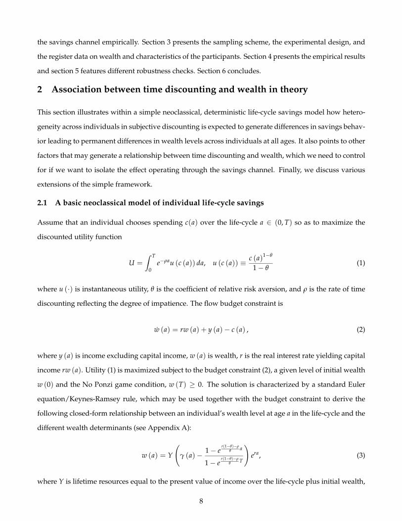
Assume that an individual chooses spending c(a) over the life-cycle a ∈ (0, T) so as to maximize the

discounted utility function

U =

ˆ T

0e−ρau (c (a)) da, u (c (a)) ≡ c (a)1−θ

1− θ(1)

where u (·) is instantaneous utility, θ is the coefficient of relative risk aversion, and ρ is the rate of time

discounting reflecting the degree of impatience. The flow budget constraint is

w (a) = rw (a) + y (a)− c (a) , (2)

where y (a) is income excluding capital income, w (a) is wealth, r is the real interest rate yielding capital

income rw (a). Utility (1) is maximized subject to the budget constraint (2), a given level of initial wealth

w (0) and the No Ponzi game condition, w (T) ≥ 0. The solution is characterized by a standard Euler

equation/Keynes-Ramsey rule, which may be used together with the budget constraint to derive the

following closed-form relationship between an individual’s wealth level at age a in the life-cycle and the

different wealth determinants (see Appendix A):

w (a) = Y

(γ (a)− 1− e

r(1−θ)−ρθ a

1− er(1−θ)−ρ

θ T

)era, (3)

where Y is lifetime resources equal to the present value of income over the life-cycle plus initial wealth,

8

while γ (a) is the share of lifetime resources received by the individual up to age a:

Y ≡ˆ T

0y (a) e−rada + w (0) , γ (a) ≡

´ a0 y (τ) e−rτdτ + w (0)

Y.

It follows from equation (3) that the wealth level of an individual w (a) starts at the given initial value

w (0) and goes to 0 at the end of the life span. The wealth level may both increase or decrease when

going through the life-cycle (higher a), and it may become negative (this happens for example, if initial

wealth is zero, w (0) = 0, and income equals zero, y (a) = 0, at the beginning of the period, in which case

wealth starts by decreasing from its initial level of zero). The main prediction follows from the wealth

equation (3) (see Appendix A):

Differences in time discounting across people (ρ) generate differences in savings behavior (c (a) profiles) that

generate inequality in wealth (cross-sectional variation in w (a)), with patient people having most wealth at all

points in the life-cycle (a) conditional on the other wealth determinants (Y, γ (a) , T, r, θ).

This shows that subjective discounting and wealth is related through the savings channel. Differences

in wealth may also arise because of differences across people in permanent income Y, time profile of

income γ (a), (expected) lifetime T, real interest rate r on savings, and the CRRA parameter θ reflecting

the degree of intertemporal substitution in consumption. These factors are potential confounders that

we would like to control for in order to isolate the role of the savings channel for the association between

time discounting and wealth inequality. If, for example, patient individuals attain higher education lev-

els and therefore higher permanent income Y, then this creates a positive relationship between patience

and wealth beyond the savings mechanism. On the other hand, more education would normally also

imply a steeper income profile, which in isolation reduces the level of wealth at a given age (due to lower

values of γ (a) in equation 3).

Note that differences in the CRRA preference parameter θ have ambiguous effects on wealth as

shown in Appendix A. A higher θ reduces wealth if r > ρ and increases wealth if r < ρ. Intuitively,

a higher θ implies a stronger preference for consumption smoothing, which flattens the consumption

profile. If the initial consumption profile is increasing (decreasing), occurring when r > ρ (r < ρ), then

this increases (decreases) consumption in the first part of life leading to lower (higher) wealth over the

life-cycle.

Note also that the theory does not imply a clear relationship between differences in patience and

the cross-sectional variation in consumption/savings levels. Patient individuals have, ceteris paribus,

9

lower consumption levels early in life and higher consumption levels later in life compared to impatient

individuals.

2.2 Extensions

Income shocks: The model only allows for deterministic variation in income over the life-cycle. This

contrasts with standard macro models of wealth inequality where income develops stochastically and is

uninsurable (De Nardi and Fella 2017). This gives variation in wealth beyond the income determinants

in the above model (Y,γ (a)) and mutes the relationship between discounting and wealth. Neverthe-

less, as described in the introduction, Krusell and Smith (1998) and others show that heterogeneity in

discounting behavior may improve the ability of macro models to explain wealth inequality.

Endogenous income and human capital formation: We have assumed exogenous income. Work effort

and human capital accumulation may well be related to impatience (Blinder and Weiss 1976), which

would affect wealth beyond the savings mechanism described in the model above. However, this does

not necessarily change the above result. Consider, for example, the following extension of the basic

model where an individual chooses the share of time spent on work ly (a), human capital formation

lh (a) and leisure lu (a) at all ages a such that ly (a) + lh (a) + lu (a) = 1. Income now depends on hours

worked and the level of human capital h (a), which depends on time spent on education:

y = f (h (a) , ly (a)) ,

h (a) = g(

h (a) , lh (a))

, h (0) given,

where f (·) and g (·) are production functions with standard properties. Finally, the utility function is

extended with utility from leisure such that

U =

ˆ T

0e−ρa [u (c (a)) + v (lu (a))] da,

where v (·) is a concave function. In this case, the first order condition for spending again gives the

standard Keynes-Ramsey rule and when combined with the budget constraint (2), we again obtain the

wealth expression (3). Hence, it is still the case in the extended model that a correlation between wealth

and subjective discounting reflects the mechanism going through the savings channel if we just condition

on the other wealth determinants, since controlling for permanent income Y and the income profile

parameter γ (a) capture the mechanisms going through income and human capital.

10

Wealth transfers: Inter vivo transfers and bequests influence wealth inequality (De Nardi 2004; Boserup

et al. 2016; 2018). The model does not explicitly include wealth transfers, but wealth transfers received

may be included in y (a), in which case the wealth expression (3) is unchanged. In a similar vein, we

may interpret c (a) as spending including transfers. From an empirical point of view, transfers only

matter for the results if they are correlated with subjective discounting (after controlling for income and

the other wealth determinants described above). If, for example, more patient individuals are also more

prone to save in order to leave bequests, this then creates a positive relationship between patience and

wealth running through savings. Thus, the main prediction is the same although savings are motivated

by giving consumption possibilities to others in the future rather than own future consumption.

Credit constraints: In the simple model, each individual may borrow and lend at a fixed interest rate

r (which could vary across individuals). A large literature has theoretically and empirically examined

the role of credit constraints for savings behavior and the persistent effects of business cycle shocks

(Zeldes 1989; Leth-Petersen 2010; Krueger et al. 2016). To see the implications of including a (hard) credit

constraint, consider the special case where consumers can never have negative wealth, i.e. w (a) ≥ 0 for

all a ∈ (0, T). Assume initial wealth w (0) is zero and income is constant, y (a) = y for all a. For patient

individuals with ρ < r, the constraint is not binding, because they would wish to have an increasing

consumption profile, implying that the wealth equation (3) still applies. For impatient individuals with

ρ > r, wealth becomes zero at all points in the life-cycle, w (a) = 0 for all a. These individuals would

prefer a decreasing consumption profile over the life-cycle, but they will end up consuming their current

income because of the credit constraint. All individuals with ρ > r, but different degrees of impatience

ρ, will then end up having the same wealth at all points in time (zero in this case). As this example

illustrates, credit constraints may imply that the most impatient individuals (ρ above some threshold)

are constrained from borrowing, and that therefore patience and wealth become uncorrelated within this

group.

A “softer” version of credit constraints is that the interest rates on loans are larger than on deposits

and that more borrowing implies higher (marginal) interest rates, reflecting that marginal lending is

less likely to be covered by collateral and more likely to be subject to default. This implies that the

marginal interest rate on additional funds for consumption is (weakly) decreasing in the level of wealth,

corresponding to r (w) where r′ (w) ≤ 0. As more impatient individuals are more willing to pay a

higher interest rate, we would ceteris paribus expect a correlation between subjective discounting and

the marginal interest rates across individuals.

11

In the empirical analysis, we use measures of both hard and soft credit constraints to examine

whether a correlation between time discounting and the propensity to be constrained exists, and we

analyze whether time discounting is associated with wealth inequality after controlling for credit con-

straints.

3 Experimental design, sample and data

Our empirical analysis combines experimental data and administrative register data. The Danish re-

search infrastructure makes this possible, whereby data can be linked across modes of data collection

using social security numbers. We use standard experimental techniques to measure time discounting

and risk attitudes for a sample drawn from the population. We then link this information at the in-

dividual level to administrative records with longitudinal information on wealth and income over the

life-cycle and other individual characteristics that may be important according to the theory in section 2.

This section describes the sampling scheme, the design and implementation of the experiment, and the

register data.

3.1 Sample and recruitment for the experiment

Respondents were recruited by sampling individuals from the Danish population register satisfying the

following two criteria: (i) born in the period 1973-1983, and (ii) residing in the municipality of Copen-

hagen (Københavns Kommune) when they were seven years old. Statistics Denmark, the central author-

ity on Danish statistics, provided a data set of all individuals who met these two sample criteria. The

data set contained names, current addresses, and civil registration numbers. All individuals in the gross

sample received a personal invitation letter in hard copy from the University of Copenhagen.6 The letter

informed subjects about a unique username and password needed to log in to a web page, the expected

time to complete the experiment, and contact information for support.7 Subjects were also informed that

the could earn money by participating in the study and that that the overall payment would depend on

their choices.

We invited a total of 27,613 subjects to participate in the online experiment that took place in February

2015.8 4,190 (15.17 percent) of all invitees logged in to our experimental platform. The vast majority

6The invitation letter and an English translation are available in Appendix B.1.7An extensive pretesting phase preceded the main experiment. This phase comprised focus groups and a series of pilot

experiments. We used these pretests to improve the task presentation, to calibrate the choice situations, and to obtain expectedtimes for completion.

8Only 424 (1.54 percent) of the 27,613 invitation letters were returned.

12

(3,717 or 88.71 percent) of subjects who did so successfully completed the experiment and received a

payment. Our analyses include a total of 3,620 subjects.9 Participation rates at this level are common for

similar experimental studies (e.g. Andersson et al. 2016 report 11%). Sections 3.3 and 5 analyze selection

into the experiment.

Subjects who followed the web link in the invitation letter arrived at a login page. After successful

login, a single page with introductory instructions appeared. These instructions described the outline

of the experiment and payment modalities. Subjects were also presented with a graphical depiction of

a wheel they had to spin at the end of the experiment. They were told that the spin of the wheel at

the end would determine the choice situation that would count for payment, and, hence, that any of

the choice situations could be picked for payment. The online experiment included three preference

elicitation tasks to measure time, risk, and social preferences. Each task was accompanied by short

video instructions and comprehension questions. The three blocks appeared in individualized random

order. Within each block, the set of choice situations was once again randomized. This paper focuses on

the time task, which is described in detail in the next subsection. In some of the analyses, we include

information from the risk task, which is described in Appendix B.4.10

The median completion time was 47 minutes. Our elicitation tasks involved real monetary incentives.

We used an experimental currency and informed the subjects that 100 points corresponded to 25 Danish

kroner (DKK).11 This provided us more flexibility for calibration of the choice situations. At the end

of the experiment, the subject spun the wheel in order to determine the choice situation relevant for

payment. The random choice situation where the wheel stopped was then displayed together with

the subject’s decision, and the points were exchanged into money. Payment was done via direct bank

transfer at the relevant date (details follow below). Possible payments considering all three tasks ranged

from 88 to 418 DKK. The average amount paid out was 245 DKK.

3.2 Measuring patience

We use standard money-earlier-or-later experiments to elicit patience. These experiments are well-suited

for implementation on an internet platform. We describe the choice tasks and how they are used to

9For the linkage between experimental and register data, it is important that the people who participated in the experimentare identical to the people who were invited. To check that the correct person participated in the experiment, the respondentswere asked to state their gender and year of birth as the first thing after logging in to the experiment. 38 respondents wereexcluded from the analysis because their stated gender and/or year of birth were not identical to the information in the registerdata. In addition, we excluded 59 persons without the required register data information (typically immigrants).

10The results reported in this paper do not use data from the social task. Results, not reported here, did not suggest anysignificant relationship between social preferences and wealth inequality.

111 USD ' 6.5 DKK at the time of the study.

13

measure patience below.

Time tasks: Our measurement of intertemporal choice behavior is based on convex time budgets (An-

dreoni and Sprenger 2012). We depict intertemporal choices graphically and present only a single al-

location choice per page. We used a total of 15 independent choice situations that differed in terms of

payment dates and interest payments.

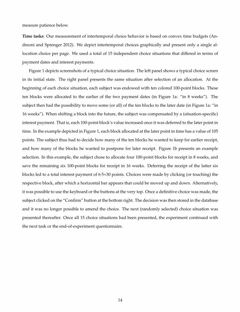
Figure 1 depicts screenshots of a typical choice situation. The left panel shows a typical choice screen

in its initial state. The right panel presents the same situation after selection of an allocation. At the

beginning of each choice situation, each subject was endowed with ten colored 100-point blocks. These

ten blocks were allocated to the earlier of the two payment dates (in Figure 1a: “in 8 weeks”). The

subject then had the possibility to move some (or all) of the ten blocks to the later date (in Figure 1a: “in

16 weeks”). When shifting a block into the future, the subject was compensated by a (situation-specific)

interest payment. That is, each 100-point block’s value increased once it was deferred to the later point in

time. In the example depicted in Figure 1, each block allocated at the later point in time has a value of 105

points. The subject thus had to decide how many of the ten blocks he wanted to keep for earlier receipt,

and how many of the blocks he wanted to postpone for later receipt. Figure 1b presents an example

selection. In this example, the subject chose to allocate four 100-point blocks for receipt in 8 weeks, and

save the remaining six 100-point blocks for receipt in 16 weeks. Deferring the receipt of the latter six

blocks led to a total interest payment of 6·5=30 points. Choices were made by clicking (or touching) the

respective block, after which a horizontal bar appears that could be moved up and down. Alternatively,

it was possible to use the keyboard or the buttons at the very top. Once a definitive choice was made, the

subject clicked on the “Confirm” button at the bottom right. The decision was then stored in the database

and it was no longer possible to amend the choice. The next (randomly selected) choice situation was

presented thereafter. Once all 15 choice situations had been presented, the experiment continued with

the next task or the end-of-experiment questionnaire.

14

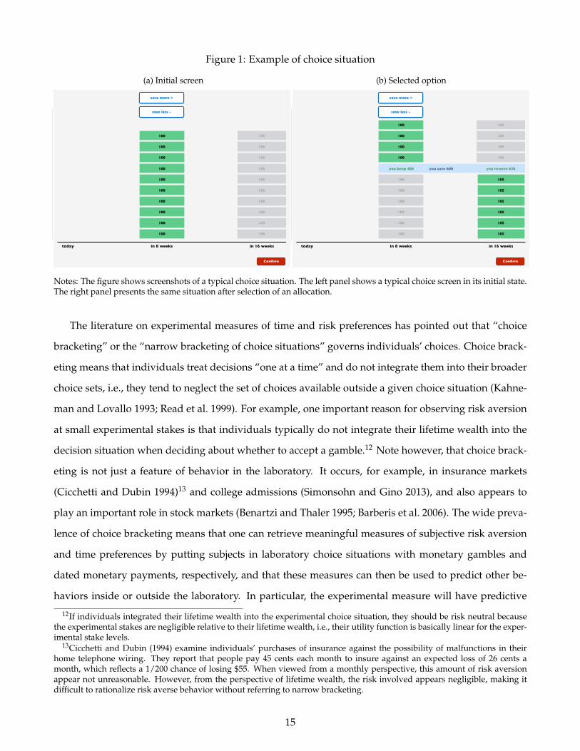
Figure 1: Example of choice situation

(a) Initial screen

100 105

100 105

100 105

100 105

100 105

100 105

100 105

100 105

100 105

100 105

today in 8 weeks in 16 weeks

Bekræft

save less -

save more +

Confirm

(b) Selected option

100 105

100 105

100 105

100 105

you keep 400 you save 600 you receive 630

100 105

100 105

100 105

100 105

100 105

100 105

today in 8 weeks in 16 weeks

Bekræft

save less -

save more +

Confirm

Notes: The figure shows screenshots of a typical choice situation. The left panel shows a typical choice screen in its initial state.The right panel presents the same situation after selection of an allocation.

The literature on experimental measures of time and risk preferences has pointed out that “choice

bracketing” or the “narrow bracketing of choice situations” governs individuals’ choices. Choice brack-

eting means that individuals treat decisions “one at a time” and do not integrate them into their broader

choice sets, i.e., they tend to neglect the set of choices available outside a given choice situation (Kahne-

man and Lovallo 1993; Read et al. 1999). For example, one important reason for observing risk aversion

at small experimental stakes is that individuals typically do not integrate their lifetime wealth into the

decision situation when deciding about whether to accept a gamble.12 Note however, that choice brack-

eting is not just a feature of behavior in the laboratory. It occurs, for example, in insurance markets

(Cicchetti and Dubin 1994)13 and college admissions (Simonsohn and Gino 2013), and also appears to

play an important role in stock markets (Benartzi and Thaler 1995; Barberis et al. 2006). The wide preva-

lence of choice bracketing means that one can retrieve meaningful measures of subjective risk aversion

and time preferences by putting subjects in laboratory choice situations with monetary gambles and

dated monetary payments, respectively, and that these measures can then be used to predict other be-

haviors inside or outside the laboratory. In particular, the experimental measure will have predictive

12If individuals integrated their lifetime wealth into the experimental choice situation, they should be risk neutral becausethe experimental stakes are negligible relative to their lifetime wealth, i.e., their utility function is basically linear for the exper-imental stake levels.

13Cicchetti and Dubin (1994) examine individuals’ purchases of insurance against the possibility of malfunctions in theirhome telephone wiring. They report that people pay 45 cents each month to insure against an expected loss of 26 cents amonth, which reflects a 1/200 chance of losing $55. When viewed from a monthly perspective, this amount of risk aversionappear not unreasonable. However, from the perspective of lifetime wealth, the risk involved appears negligible, making itdifficult to rationalize risk averse behavior without referring to narrow bracketing.

15

power to the extent to which subjective preferences measured in the experiment reveal an individual’s

general tendency to value risk and time in other domains.

Choice situations in our experiment involved three different payment dates: “today”, “in 8 weeks”,

and “in 16 weeks”. Combinations of all three payment dates were used. We decided to state delays in

terms of weeks (instead of months) to prevent possible weekday effects. The compiled list of transactions

were then sent electronically to the bank for implementation of the payout. Subjects knew that the

payment was initiated either on the same day, or exactly 8 or 16 weeks later. Hence, the payment dates

shown on the screen refer to the points in time where the transactions were actually initiated. It took one

day to transfer the money to the subject’s “NemKonto”, which is a publicly registered bank account that

every Danish citizen possesses and which is typically used as the salary account. Exceptions were non-

banking days, such as weekends or holidays. In this case, the transaction occurred on the subsequent

banking day.

The interest rates applied varied across choice tasks. For example, the five choice tasks asking sub-

jects to choose between receiving payments in 8 weeks or 16 weeks had rates of return in the interval 5-25

percent (amounting to annualized interest rates in the range of 34-282 percent). This range of interest

rates is similar to those used in the other studies reviewed in the introduction. Moreover, Appendix B.3

shows that the distribution of choices made by the participants in our internet experiment is very similar

to the choice distribution in the lab experiment of Andreoni and Sprenger (2012). Potentially, discount

rates for larger stake sizes would be lower due to the so-called “magnitude effect” (e.g. Frederick et al.

2002). However, for our purpose of examining the link between patience and wealth inequality, only

the ordering of the subjects according to their time discounting is relevant. The magnitude effect would

arguably change the size of the elicited discount rates, but there is no reason to believe that it would

change the relative position of the subjects.

Patience measure: We use a simple patience index based on the mean number of blocks saved for later

receipt to measure an individual’s degree of patience. We compute the patience index for the five choice

situations in the time frame with allocations between t1 = 8 weeks and t2 = 16 weeks:14

φpatience = mean( z1

10, ...,

z5

10

), (4)

where zi denotes the number of blocks saved in task i, and where we divide each choice by the total

number of blocks so that φpatience ∈ [0, 1]. Higher values of φpatience indicate greater patience. Due to the

14The allocations are labeled choiceId ∈ {11, ..15} in Table A1 of Appendix B.2.

16

discreteness of our measures (10 blocks to allocate in each of the 5 choice situations), our index can take

values in steps of 1/50. By construction, censoring occurs at both ends of the scale, making it impossible

to detect lower and higher discount rates than those offered in the experiment. Figure 2 depicts the

cumulative distribution of the patience index. It reveals substantial heterogeneity across the individuals

in the sample with the exception of the top end of the distribution where 18 percent of the individuals

saved all blocks in all five choice situations. Figure 2 also shows tertile cut-off points, which are used in

the empirical analyses to split individuals into high, medium, and low patience groups in order to be

able to illustrate the differences in outcomes across these groups graphically.

In the robustness section 5.2, we show that our results are robust to using the choices based on the

time frames “today” versus “in 8 weeks” and “today” versus “in 16 weeks”, to basing the aggregation

of individual choices on the median instead of the mean, and to ranking the individuals according to

structurally estimated discount factors obtained from a random utility model estimated on the choice

data.

Figure 2: Distribution of the patience index

0

.1

.2

.3

.4

.5

.6

.7

.8

.9

1

CD

F of

pat

ienc

e

0 .1 .2 .3 .4 .5 .6 .7 .8 .9 1Patience

Notes: The figure shows the cumulative distribution of the patience index computed from expression (4) using theexperimental data. The red lines indicate tertile cut-off points.

3.3 Register data information on wealth and other characteristics

The choice data from the experiment is linked at the individual level with administrative register data

17

at Statistics Denmark.15 The register data contains demographic characteristics and longitudinal infor-

mation about annual income and values of assets and liabilities at the end of each year for each individ-

ual. The income and wealth information is based on third party reports to the Danish tax authorities.

For instance, employers report earnings, government institutions report transfer payments, and banks,

mortgage institutions, mutual funds, and insurance companies report values of assets and liabilities.

The value of assets includes bank deposits, market value of listed stocks, bonds and mortgage deeds

in deposit, and value of property assessed by the tax authorities using land and real estate registries.

The value of liabilities includes all debt except debt to private persons. The data contains information

about adult individuals (age≥18) over the period 1980-2015. Wealth accumulated in pension accounts

and estimated car values are available as of 2014. In the robustness section, we show that the inclusion

of these components has minor effects on the main results.

The Danish wealth data has been used previously for research examining credit constraints (Leth-

Petersen 2010; Kreiner et al. 2018), retirement savings (Chetty et al. 2014a), accuracy of survey responses

(Kreiner et al. 2015), effects of bequests on wealth inequality (Boserup et al. 2016), and effects of wealth

taxation on wealth accumulation (Jakobsen et al. 2018). Wealth inequality has been reasonably stable

in Denmark over the 35-year observation period, with the top 10% richest owning between 50 and 80

percent of wealth depending on the definition of wealth and the sample considered (Boserup et al. 2016;

Jakobsen et al. 2018).

Table 1 provides summary statistics for our respondents (column a), and compares their character-

istics to those of non-respondents (columns b-c) and a 10% random sample of the full population of

this age group (columns d-e). The respondents’ median wealth level is slightly higher than the median

of their annual gross income. People in the bottom 10% of the distribution have negative net wealth.

Percentile 95 of the wealth distribution is about five times the median. The corresponding ratio for the

income distribution is less than 2, showing that wealth is much more concentrated than income. The

respondents are slightly older, less likely to be single, and slightly more highly educated compared to

non-respondents. Wealth and income of the respondents are higher throughout the distributions. In

general, the differences are smaller when we compare respondents to the random sample of the popu-

lation. For example, the difference in median wealth is less than 1 percent. Section 5 provides evidence

15In practice, the experimental data was merged with the administrative data by Statistics Denmark using a link betweenusernames provided in the invitation letters and the civil registration numbers of the individuals. The final data set where thepersonal identifiers are removed is stored on servers at Statistics Denmark enabling data analysis through a secure interface.The participants were not informed that the data from the experiment would be linked with the administrative register data.The Danish Data Protection Agency approved the research project and this procedure.

18

suggesting that our main results are not very sensitive to the differences in sample composition shown

in Table 1.

Table 1: Means of selected characteristics

(1) Respondents vs. non-respondents (2) Respondents vs. 10% of population

(a) (b) (c) (d) (e)Respondents Non-respondents Difference, (a)-(b) Population Difference, (a)-(d)

Age 37.32 36.46 0.86 37.37 -0.05Woman (=1) 0.50 0.49 0.01 0.51 -0.01Single (=1) 0.28 0.38 -0.10 0.28 0.00Dependent children (=1) 0.61 0.57 0.04 0.63 -0.02Years of education 14.89 14.16 0.73 14.64 0.25Gross income distributionp5 135745 98974 36772 130343 5402p25 287472 234966 52506 270900 16572p50 383040 341611 41429 360132 22908p75 484472 434678 49795 456263 28209p95 720178 654999 65179 700517 19661Wealth distributionp5 -337615 -351123 13507 -241803 -95812p25 93898 48919 44978 144177 -50280p50 487002 317400 169602 483217 3785p75 1066942 800074 266868 972420 94522p95 2397821 2024448 373373 2254289 143532

Observations 3620 23626 27246 67539 71159

Notes: Variables are based on 2015 values. The random 10% sample of the Danish population is drawn from individuals bornin the same period (1973-1983) and not included in the gross sample (i.e., did not live in the capital city of Copenhagen or thesurrounding area when they were seven years old). (=1) indicates a dummy variable taking the value 1 for individuals whosatisfy the description given by the variable name. Wealth denotes the value of real estate, deposits, stocks, bonds, mortgagedeeds in deposit, cars, and pension accounts minus all debt except debt to private persons. The tax assessed values of housingis adjusted by the average ratio of market prices to tax assessed values among traded houses of the same property class andin the same location and price range. Gross income refers to annual income and excludes capital income. The table includesindividuals for whom a full set of register variables is available.

4 Empirical results

In this section, we present the empirical findings. First, we derive the overall association between time

discounting and wealth inequality. Informed by theory, we then introduce a large number of control

variables with the aim of isolating an association between patience and wealth inequality operating

through the savings channel. We also analyze whether the elicited patience predicts if individuals are

among the top 10% of the wealthiest, and we present a large number of robustness analyses.

19

4.1 Overall association between time discounting and wealth inequality

Most of our analysis is based on measuring the relationship between individuals’ elicited time discount-

ing and their positions in the wealth distribution, measured by the individual’s percentile rank in the

within cohort×time distribution of the sample (e.g. Chetty et al. 2014b). This measure has several advan-

tages: it compares an individual’s wealth with the wealth of others from the same cohort and at the same

point in time, thereby controlling for life-cycle and time trends in wealth; it works well with zero and

negative observations that are common in wealth data; and it is a very robust measure (insensitive to

outliers and unaffected by monotone transformations of the underlying data). Figure 3a presents graph-

ical evidence of the association between the elicited patience measure and the position in the wealth

distribution of the individuals in the sample for each year in the period 2001-2015. In the figure, the

sample is split into three equally sized groups according to the size of the patience measure such that the

“High” group includes the most patient individuals in the sample, “Low” the least patient individuals

and “Medium” includes individuals with patience measures between the “High” and “Low” groups.

The figure shows that the individuals’ patience ordering predicts the position in the wealth distribution,

so that the group average of the most patient individuals is consistently at the highest position in the

wealth distribution, followed by the group with medium patience, and with the most impatient individ-

uals on average attaining the lowest position in the wealth distribution. Comparing the percentile rank

position among the most patient with the rank position among the least patient in Figure 3a reveals a

difference of about 6-7 wealth percentiles throughout the 15 year period that the data spans.

20

Figure 3: Time discounting, educational attainment, and wealth inequality

(a) Patience and position in the wealth distribution

Impatient

Middle

Patient

45

46

47

48

49

50

51

52

53

54

55

Wea

lth p

erce

ntile

rank

2001 2003 2005 2007 2009 2011 2013 2015Year

Low Medium High

(b) Patience vs. education and parental wealth

40

42

44

46

48

50

52

54

56

58

60

Wea

lth p

erce

ntile

rank

Medium

Patience Educational attainmentParental wealth 95% CI

Low High

Notes: Panel a shows the association between elicited patience and the position in the wealth distribution in the period 2001-2015. The position in the distribution is computed as the within cohort×time percentile rank. The sample is split into threeequally sized groups according to the tertiles of the patience measure such that “High” includes the 33 percent most patientindividuals in the sample, “Low” the 33 percent most impatient individuals and “Medium” the group in between the “High”and “Low” groups. Cut-offs for the patience groups are: Low [0.0, 0.5]; Medium [0.5, 0.8]; High [0.8, 1.0]. Panel b compares thepatience-wealth association to the education-wealth association and to the parental wealth-wealth association. The subject’swealth is measured in 2015, educational attainment equals years of completed education, and parental wealth is measuredwhen the subject was eighteen years old. The individuals in the sample are split into three equally sized groups according topatience, years of education, and parents’ position in their wealth distribution, respectively. Cut-offs for the education groups(years): Low [8, 14]; Medium [14, 16.5]; High [16.5, 21] where the numbers refer to years of completed education.

To assess the magnitude of the association between patience and wealth inequality, we compare it

to the association between educational attainment levels and wealth inequality. Huggett et al. (2011) ar-

gue that educational attainment is one of the most important factors contributing to lifetime inequality.

Figure 3b splits the sample into three equally sized groups according to educational attainment as mea-

sured by the number of years of completed education. The group with least education has completed

8-14 years of education, while the group with most education has completed 16.5-21 years of education.

Comparing the groups with the lowest and the highest level of educational attainment shows a differ-

ence of six to seven wealth percentiles, which is comparable to the association with patience. We also

compare the association between patience and wealth to the relationship between parental wealth and

child wealth. It is well-known from the intergenerational literature that parental wealth is a strong pre-

dictor of child wealth (Charles and Hurst 2003; Clark and Cummins 2014; Adermon et al. 2018). Figure

3b also splits the sample into three equally sized groups according to parental wealth. Individuals with

21

parents in the top 1/3 of the parental wealth distribution are positioned 15 percentiles higher in the child

wealth distribution than individuals with parents in the lowest 1/3 of the parental wealth distribution.

In other words, based on the bivariate correlations, heterogeneity in time discounting and in education

appear to be roughly equally important for individuals’ wealth rank, whereas parental wealth is roughly

twice as important.

4.2 Isolating the savings channel

4.2.1 Role of education and income

The bivariate association between patience and wealth inequality in Figure 3 is potentially caused by

higher savings propensities of patient individuals as predicted by life-cycle savings theory, but it could

also exist because patient individuals invest more in education, thereby attaining higher income and

wealth, or because of the other mechanisms described in the theory section 2. We therefore turn to

multivariate regressions and sequentially add control variables with the aim of isolating an association

between patience and wealth inequality operating through the savings channel. We focus on the wealth

percentile rank at the end of the observation period in the regressions. At this point in the life-cycle,

individuals have completed their education and income is arguably a good proxy for permanent income

(Haider and Solon 2006).16 The results are presented in Table 2. Column 1 presents the result from a

simple bivariate regression of the wealth percentile on the patience measure. It shows that moving from

the lowest to the highest level of patience in the sample is associated with a difference of some eleven

wealth percentiles, and this association is statistically significant at the 0.1 percent level.

16We also ran regressions with wealth data covering the whole period 2001-2015. The results are presented in section 5.3 andconfirm the results presented in Table 2.

22

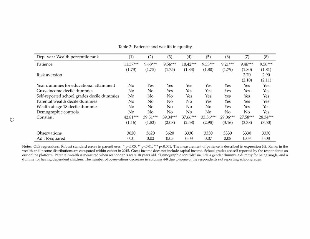
Table 2: Patience and wealth inequality

Dep. var.: Wealth percentile rank (1) (2) (3) (4) (5) (6) (7) (8)

Patience 11.37*** 9.68*** 9.56*** 10.42*** 9.33*** 9.21*** 9.46*** 9.50***(1.73) (1.75) (1.75) (1.83) (1.80) (1.79) (1.80) (1.81)

Risk aversion 2.70 2.90(2.10) (2.11)

Year dummies for educational attainment No Yes Yes Yes Yes Yes Yes YesGross income decile dummies No No Yes Yes Yes Yes Yes YesSelf-reported school grades decile dummies No No No Yes Yes Yes Yes YesParental wealth decile dummies No No No No Yes Yes Yes YesWealth at age 18 decile dummies No No No No No Yes Yes YesDemographic controls No No No No No No No YesConstant 42.81*** 39.51*** 39.34*** 37.66*** 33.36*** 29.06*** 27.58*** 28.34***

(1.16) (1.82) (2.08) (2.58) (2.98) (3.16) (3.38) (3.50)

Observations 3620 3620 3620 3330 3330 3330 3330 3330Adj. R-squared 0.01 0.02 0.03 0.03 0.07 0.08 0.08 0.08

Notes: OLS regressions. Robust standard errors in parentheses. * p<0.05, ** p<0.01, *** p<0.001. The measurement of patience is described in expression (4). Ranks in thewealth and income distributions are computed within-cohort in 2015. Gross income does not include capital income. School grades are self-reported by the respondents onour online platform. Parental wealth is measured when respondents were 18 years old. “Demographic controls” include a gender dummy, a dummy for being single, and adummy for having dependent children. The number of observations decreases in columns 4-8 due to some of the respondents not reporting school grades.

23

Patient individuals may be more prone to have delayed incomes by choosing longer education. Con-

versely, education may also contribute to patience. The data shows a significant positive correlation be-

tween patience and educational attainment. The average years of education for the low patience group

is 14.3, while it is 15.3 years for the high patience group. In this way, education is also a marker for pa-

tience as suggested by Lawrance (1991). Column 2 includes flexible dummies for educational attainment

as control variables. The coefficient on the patience measure decreases somewhat, but it is still large with

a value of 10 percentiles. Thus, the relationship between patience and wealth exists beyond education.

According to the basic theory, differences across individuals in the level of permanent income and in

the time profiles of income are important for the cross-sectional variance in wealth. A higher permanent

income is associated with a higher position in the wealth distribution at all ages. However, holding total

lifetime income fixed, an increasing profile of income leads to a lower position in the wealth distribution

at all ages compared to a flat income profile. Figure 4a plots the position in the within-cohort income

ranks for the respondents at different ages and separately for the three patience groups defined in Figure

3. The panel shows that the most patient group on average has a steeper income profile over the age

interval 18-40. They start out being ranked lower in the income distribution than the less patient groups,

but at age 40 they are positioned about 6 percentiles higher than the low patience group, suggesting that

these individuals have a higher level of permanent income. It turns out that the controls for educational

attainment capture these differences in timing of income and levels of permanent income to a large

extent. To see this, consider Figure 4b, which plots coefficients from regressions of the (within age group

and year) labor income percentile rank on the patience group dummies, where “low patience” is the

reference group, and a fully flexible set of dummies for years of completed education. Panel b shows

that the differences across the three patience groups in the level and the slope of income are washed

out by controlling for educational attainment. This suggests that including a detailed set of dummies

for educational attainment in Table 2, column 2, adequately controls for the differences in permanent

income and in timing of income observed in the raw data.

24

Figure 4: Relationship between discounting behavior and income over the life-cycle

(a) Unconditional

Patient

Middle

Impatient

45

46

47

48

49

50

51

52

53

54

55

Inco

me

perc

entil

e ra

nk

18 20 22 24 26 28 30 32 34 36 38 40Age

Low Medium High

(b) Conditional on education

Patient (right capped spikes)Middle (left capped spikes)Impatient (base group)

-6

-4

-2

0

2

4

6

8

10

Inco

me

perc

entil

e ra

nk

18 20 22 24 26 28 30 32 34 36 38 40

Age

Notes: Panel a shows the position in the within-age-group-and-year labor income distribution for the respondents over the life-cycle separately for three patience groups. The sample is split into three equally sized groups according to the tertiles of thepatience measure such that “High” includes the 33 percent most patient individuals in the sample, “Low” the 33 percent mostimpatient individuals and “Medium” the group in between the “High” and “Low” groups. Cut-offs for the patience groupsare: Low [0.0, 0.5]; Medium [0.5, 0.8]; High [0.8, 1.0]. Panel b plots coefficients from regressions of ’within-age-group-and-yearlabor income percentile rank’ on the patience groups and fully flexible “years of education” dummies. “Middle” and “Patient”indicate the “Medium” and “High” patience groups, respectively. “Low” patience is the base group. Capped spikes represent95% CI. The panel shows that the income paths for the three patience groups are leveled out when controlling for education.

In column 3 of Table 2, we further control for income differences by including decile dummies for the

position in the within-cohort income distribution (gross income excluding capital income). The inclusion

of these dummies hardly affects the parameter on the patience measure.17 Recent evidence suggests that

cognitive ability is correlated with time discounting and risk attitudes (Dohmen et al. 2010).18 In column

4, we add decile dummies for school grades. This increases the estimate of the patience parameter.

4.2.2 Controlling for parental wealth and initial wealth

Wealth accumulation may also be influenced by transfers from parents (Boserup et al. (2016)), which may

help explain why wealth is more concentrated than income (De Nardi 2004). We do not directly observe

bequests and inter vivo transfers in the data. However, if the variation in family transfer payments across

17We have also constructed a figure corresponding to Figure 3a, but where wealth is normalized by income in 2015 beforecalculating the position in the wealth distribution. This graph also shows that the most patient individuals are persistentlylocated higher in the distribution of wealth-income ratios than the less patient individuals.

18The association between risk preferences and ability has recently been questioned (Andersson et al. 2016).

25

individuals is a function of parental wealth, this information can be used as a proxy. Column 5 includes

decile dummies for the within-cohort parental wealth measured when individuals are 18 year old. The

coefficient on the patience measure remains largely unchanged, indicating a nine percentile increase in

the wealth rank associated with moving from the bottom to the top of the patience distribution.19

Theoretically, initial wealth is another potential confounding factor if we want to isolate the role of

the savings channel. Figure 5 plots the percentile rank of wealth in year 2015 less wealth holdings at

age 18 (the age of majority) against the wealth percentile rank in year 2015. We compound wealth at

age 18 with a relatively high real interest rate (5 percent) to make sure that we do not underestimate the

potential effect of initial wealth. The graph lies close to the 45 degree line implying that initial wealth

has a negligible effect on the position in the wealth distribution in year 2015, in line with the evidence in

Boserup et al. (2018). Table 2, column 6 includes decile dummies for the within-cohort wealth rank at age

18. Consistent with the graphical evidence, the inclusion of these controls does not affect the parameter

on patience in any important way.

Figure 5: Importance of initial wealth at age 18

0

20

40

60

80

100

Wea

lth ra

nk,

subt

ract

ing

com

poun

ded

initi

al w

ealth

0 20 40 60 80 100Wealth percentile rank

95% CI Local polynomial regression Diagonal

Notes: Local polynomial regression of the percentile rank of wealth in 2015 less wealth holdings at age 18 on wealth percentilerank (2015). Wealth at age 18 is compounded by a real interest rate of 5 percent.

19We obtain the same result if we confine the sample to individuals where both parents are alive in 2015, see Appendix C.1.This rules out that wealth differences are driven by inheritance from parents.

26

4.2.3 Risk preferences and demographic controls

We also elicited risk preferences in the experiment. Section 2 shows that the CRRA parameter has am-

biguous effects on wealth depending on the relative size of the rate of time preference and the real

interest rate on savings. Irrespective of the theoretical association between risk aversion and wealth,

existing studies suggest that risk aversion and patience are correlated (e.g. Leigh 1986; Anderhub et al.

2000; Eckel et al. 2005). In our data, elicited risk aversion is also correlated with elicited patience, and risk

aversion could therefore potentially confound the association between wealth and patience. Column 7

includes our experimental measure of risk aversion among the control variables. Again, our parameter

of interest is left virtually unchanged and remains strongly significant.

Column 8 includes a set of additional demographic controls for gender, single status, and dependent

children. This does not impact the patience parameter estimate either.

4.2.4 Role of financial markets

So far, we have focused on controlling for heterogeneity in economic resources entering into the

intertemporal budget set of the individuals. In this section, we focus on potential differences in the slope

of the budget constraint. Theory predicts that relatively impatient people wish to borrow more and,

therefore, face a higher risk of being credit constrained. This potential relationship between patience

and credit constraints may contribute to the propagation of business cycle shocks and the impact of

stimulus policy (Carroll et al. 2014; Krueger et al. 2016). It also implies that credit constraints can mute

the relationship between patience and wealth as shown in section 2. In this section, we analyze whether

the elicited degree of patience in the experiment is related to credit constraint tightness measured with

the register data, and whether this influences the relationship between patience and wealth. We also use

the register data to control for heterogeneity in asset returns. Finally, we address whether it might be the

case that the time discounting elicited in the experiment only measures market interest rates faced by

the subjects rather than heterogeneity in true time discounting.

Credit constraints are inherently difficult to measure, as they are defined by the shadow value of

liquidity, which is not observed. We follow the previous literature and apply two different proxies for

liquidity constraints. Our first measure is a dummy variable for the respondent holding liquid financial

assets corresponding to less than one month’s disposable income. This measure has routinely been

applied in the literature (e.g. Zeldes 1989; Johnson et al. 2006; Leth-Petersen 2010). However, it is not

necessarily a good measure of the shadow value of liquidity, as people can have different access to

27

credit and therefore effectively face constraints that affect them with different intensity even if they are

otherwise observationally equivalent. Therefore, we also use a measure capturing the interest rate on

marginal liquidity (local slope of the budget set). This ’marginal interest rate’ is based on account level

data with information about debt, deposits, and interest payments during the year. We calculate an

average interest rate for each account of an individual. For people with debt accounts, we select the

highest interest rate among debt accounts as the marginal interest rate. For people without debt, we

select the lowest interest rate among their deposit accounts based on the logic that this is the cheapest

source of liquidity. Kreiner et al. (2018) show that the computed interest rates match actual interest

rates set by banks and that this measure of liquidity constraint tightness improves the ability to predict

spending responses to a stimulus policy. Details about the construction of the marginal interest rate and

its distribution are presented in Appendix C.2 and Kreiner et al. (2018).

Figure 6: Patience and the probability of being credit constrained

6

6.5

7

7.5

8

8.5

9

Mar

gina

l int

eres

t rat

e (p

erce

nt)

25

30

35

40

45

50

Sha

re o

f liq

uidi

ty c

onst

rain

ed s

ubje

cts

(per

cent

)

Medium

Left axis Right axis 95% CI

Low High

Notes: The white bars show the association between elicited patience and the propensity to hold liquid assets worth less thanone month’s disposable income in 2014. The sample is split into three equally sized groups according to the tertiles of thepatience index such that “High” includes the 33 percent most patient individuals in the sample, “Low” the 33 percent mostimpatient individuals and “Medium” the group in between the “High” and “Low” groups. Cut-offs for the patience groupsare: Low [0.0, 0.5]; Medium [0.5, 0.8]; High [0.8, 1.0]. The grey bars show the association between elicited patience and themarginal interest rate in 2014 for the three patience groups.

Figure 6 illustrates the association between patience and the indicators for being affected by con-

straints. As above, we split the sample into three equally sized groups according to the magnitude of

the experimental patience measure and calculate the fraction observed with liquid assets worth less than

28

one month’s disposable income (white bars) and the average of the marginal interest rates faced by the

individuals (grey bars). The graph shows that 33 percent of the individuals in the most patient group

are observed with a low level of liquid assets in real-life compared to 45 percent with a low level of liq-

uid assets in the least patient group. This is consistent with the theoretically motivated proposition that

impatient people save less and hence are more likely to end up in a situation where they are affected by

liquidity constraints. Turning to the association between the patience measure and the marginal interest

rate, the overall pattern is confirmed. The most patient group faces, on average, a marginal interest rate

of slightly less than 7 percent, while the least patient group faces a marginal interest rate of about 8.5

percent.

We compute the two measures of credit constraints before collecting the experimental data about

patience. This leaves open the possibility that elicited patience is a response to an adverse shock, which

has led a patient individual to drive down his liquid assets and, consequently, transitorily behave as

if he were impatient. Figure 7 shows the fraction of people who are recorded with liquid assets worth

less than one month’s disposable income for the period 2001-2015 for each of the three patience groups.

The graph shows that the propensity to be observed with low levels of liquid assets generally declines

for all three groups over time. This reflects the fact that people in the sample are in the early stages of

their life-cycle and accumulate more assets as they grow older. More importantly, the figure shows that

in each of the 15 years the share of credit constrained individuals is considerably larger among the 1/3

least patient subjects compared to the 1/3 most patient ones. Such persistence is difficult to rationalize

with short term shocks.

29

Figure 7: Prevalence of liquidity constraints across levels of patience, 2001-2015

Patient

Middle

Impatient

30

35

40

45

50

55

60

Sha

re o

f liq

uidi

ty c

onst

rain

ed s

ubje

cts

(per

cent

)

2001 2003 2005 2007 2009 2011 2013 2015Year

Low Medium High

Notes: The figure shows the association between elicited patience and the frequency of individuals within each patience groupwho are observed with liquid assets corresponding to less than one month’s disposable income. The sample is split into threeequally sized groups according to the tertiles of the patience index such that “High” includes the 33 percent most patientindividuals in the sample, “Low” the 33 percent most impatient individuals and “Medium” the group in between the “High”and “Low” groups. Cut-offs for the patience groups are: Low [0.0, 0.5]; Medium [0.5, 0.8]; High [0.8, 1.0].

To investigate how direct measures of constraints might affect the position in the wealth distribution,

we split the sample according to the dummy variable indicating whether the respondents hold liquid

assets worth more or less than one month’s disposable income and repeat the regressions from Table

2 separately for the two groups. The results are reported in Table 3. Columns 1 and 2 report results

from the subsample holding liquid assets worth more and less, respectively, than one month’s dispos-

able income. We include the full set of controls that were also included in Table 2, column (8) in these

regressions. Consistent with theory, we find that elicited patience is no longer predictive of the wealth

percentile rank for the subgroup where credit constraints are likely to be binding, column (2). How-

ever, the association between patience and wealth is much stronger than in the pooled sample for the

group who are unlikely to be affected by constraints, column (1), cf. Table 2. In fact, the results pre-

sented in Table 3, column (1) suggest that moving from the lowest level of patience to the highest level

is associated with an increase in the position in the wealth distribution of more than 12 percentiles. The

dummy variable for holding high/low levels of liquid assets arguably does not capture the entire effect

of constraints, since the intensity of constraints is likely to vary within the two groups. We include the

30

marginal interest rate among the regressors to control for the intensity of constraints in columns 3 and 4.

Recent evidence suggests that some individuals are better at obtaining high returns on savings (Fagereng

et al. 2018). Therefore, we also include asset returns among the regressors. It is computed for each in-

dividual by adding dividend income received in 2014 to realized and unrealized capital gains/losses

from the start to the end of the year, and then dividing by the market value of the assets. For both the

high (column 3) and the low (column 4) liquid asset groups, the parameter on the marginal interest rate

is significant and negative such that a higher marginal interest rate is associated with a lower wealth

rank. The asset return coefficient is positive in both cases. The inclusion of the marginal interest rate

and asset returns mutes the parameter estimate on patience, but it remains highly significant and of a

magnitude indicating that the most patient person is ranked about nine wealth percentiles higher than

the least patient person in the sample consisting of people holding liquid assets corresponding to at least

one month’s disposable income. The parameter estimate on patience remains insignificant for the low

liquid asset group. The evidence presented in Table 3 is consistent with the theoretical conjecture that

credit constraints mute the relationship between patience and the position in the wealth distribution.

Moreover, when controlling for the marginal interest rate and the asset returns, which arguably capture

the slope of the intertemporal budget constraint, we still find a strong association between patience and

wealth inequality.

These findings also speak to the issue about whether differences in elicited time discounting simply

reflect variation in real-life market interest rates facing the individuals who participated in the online ex-

periments (Frederick et al. 2002, Krupka and Stephens 2013). The fact that patience significantly predicts

the wealth percentile rank after controlling directly for the market interest rate suggests that discounting

behavior elicited with experimental methods not only reflects market interest rates, but also differences

in time preferences.

31

Table 3: Wealth percentile rank, patience and credit constraints

Dep. var.: Wealth percentile rank (1) (2) (3) (4)Liquid Assets: High Low High Low

Patience 12.31*** -1.11 8.83*** -0.44(2.47) (2.41) (2.34) (2.33)

Risk aversion 5.75* -1.82 3.49 -1.72(2.77) (2.91) (2.63) (2.87)

Interest rate on liquidity -1.68*** -0.72***(0.11) (0.08)

Rate of return on stocks 0.17 1.09*(0.20) (0.52)

Year dummies for educational attainment Yes Yes Yes YesGross income decile dummies Yes Yes Yes YesSelf-reported school grades decile dummies Yes Yes Yes YesParental wealth decile dummies Yes Yes Yes YesWealth at age 18 decile dummies Yes Yes Yes YesDemographic controls Yes Yes Yes YesConstant 21.57*** 41.94*** 43.73*** 51.72***

(5.90) (4.38) (5.64) (4.36)

Observations 2017 1274 2017 1274Adj. R-squared 0.07 0.03 0.18 0.08

Notes: OLS regressions. Robust standard errors in parentheses. * p<0.05, ** p<0.01, *** p<0.001. Columns 1 and 3 reportestimation results on the subsample of respondents who are recorded holding liquid assets worth more than one month’sdisposable income in 2014. Columns 2 and 4 report estimation results on the subsample holding liquid assets worth less thanone month’s disposable income in 2014. Percentile ranks in the wealth and income distributions are computed within-cohortin 2015. Marginal interest rates and asset returns are measured in 2014. Gross income does not include capital income. Schoolgrades are self-reported by the respondents on our online platform. Parental wealth is measured when respondents were18 years old. “Demographic controls” include three variables: a gender dummy, a dummy for being single, and a dummy forhaving dependent children. The number of observations included in this table is slightly lower than the number of observationsincluded in Table 6. This is because the register data does not allow the construction of the dummy indicator for liquidityconstraints because disposable income is recorded to be negative. Furthermore, the number of observations is reduced whenentering the marginal interest rate, as some of the detailed account-specific information is missing for some individuals.

4.3 The top 10 percent wealthiest

A sizable literature has studied the concentration of wealth at the top of the distribution. For example,

Piketty and Saez (2014) find that the share of total wealth owned by the wealthiest ten percent has been in

the range 60-90 percent over the last 150 years in the US and Europe. In order to examine whether there

is an association between our patience measure and the propensity to be in the top end of the wealth dis-

tribution, Figure 8 displays the fraction of respondents who belong to the wealthiest ten percent within

the three patience groups defined in the previous section. The figure shows that about seven percent in

the least patient group are among the wealthiest ten percent in the sample, whereas 14 percent of the

individuals categorized to be among the most patient individuals belong to the wealthiest ten percent in

the sample. Again, we compare the association with the corresponding associations for education and

32

parental wealth. Among the 1/3 of individuals with the highest level of education, 15 percent belong

to the ten percent wealthiest, whereas 5 percent is so among the 1/3 with the lowest level of education.

Similarly, about 16 percent of the children among the top third in terms of parental wealth belong to the

wealthiest ten percent, whereas 6 percent among the bottom 1/3 in terms of parental wealth belong to

the top 10 percent most wealthy individuals in the sample. Thus, while the association between patience

and the propensity to be among the wealthiest ten percent is not quite as pronounced, it is of the same

order of magnitude as the association between education and the position in the wealth distribution, and

the picture is roughly similar when comparing to the association between being among the wealthiest

ten percent and parental wealth. In Appendix C.3, we show regressions corresponding to the regressions

presented in Table 2, but where the dependent variable is a dummy variable indicating whether the re-

spondent belongs to the wealthiest ten percent. The results show that patience is statistically significant,

also when controlling for the same set of control variables as in Table 2. Due to the limited sample size,

it is impossible to credibly examine how patience is related to the propensity to belong to the group of

the very wealthy, say, to the top 0.1%.

33

Figure 8: Relationship between patience and being among the top 10% wealthiest

2

4

6

8

10

12

14

16

18

Sha

re in

top

10%

(per

cent

)

Medium

Patience Educational attainmentParental wealth 95% CI

Low High

Notes: The black bars show the association between elicited patience and the propensity to be among the wealthiest ten percentin the sample (top ten percent in the within-cohort wealth distribution, 2015). The sample is split into three equally sized groupsaccording to the tertiles of the patience index such that “High” includes the 33 percent most patient individuals in the sample,“Low” the 33 percent most impatient individuals and “Medium” the group in between the “High” and “Low” groups. Cut-offs for the patience groups are: Low [0.0, 0.5]; Medium [0.5, 0.8]; High [0.8, 1.0]. The grey bars show the association betweenthe propensity to be among the wealthiest ten percent in the sample and educational attainment, where the individuals in thesample are split into three equally sized groups according to how many years of education they have completed. Cut-offs forthe education groups (years): Low [8, 14]; Medium [14, 16.5]; High [16.5, 21] where the numbers refer to years of completededucation. The white bars show the association between the propensity to be among the wealthiest ten percent in the sampleand parental wealth, where the individuals in the sample are split into three equally sized groups according to their parents’positions in the parental wealth distribution. Parental wealth is measured when the subject was eighteen years old.

5 Additional analyses and robustness checks

This section presents a series of robustness checks corroborating our main findings. First, we use an

alternative data source where time discounting was elicited by survey in 1973 and reproduce some of our

main results, thereby addressing the pertinent question of whether it is important for our key results that

individual time discounting in the experiment is measured at the end of the observation period. Second,

we consider other ways of measuring patience in the experiment. Finally, we examine the robustness of

our core results to the definition of wealth, to the observation period, and to selection into participation

in the experiment.

34

5.1 Does time discounting measured early in the life-cycle predict future position in the

wealth distribution?

This section uses data from the Danish Longitudinal Survey of Youth (DLSY). The DLSY survey contains

a crude measure of time discounting collected in 1973 for a sample consisting of 2,550 individuals from

the 1952-1955 cohorts.20 The survey data is merged with administrative records covering the same pe-

riod as the core analysis. In this way we examine whether an alternative measure of time discounting

collected when individuals are 18-21 years old is predictive of future inequality in wealth observed when

they are about 45-60 years old. The respondents in the 1973 survey were asked, among other things, the

following question: If given the offer between the three following jobs, which one would you choose? (i) A job with

an average salary from the start. (ii) A job with low salary the first two years but high salary later. (iii) A job with

very low salary the first four years but later very high salary. We interpret this question about the preference

over the timing of income streams as a proxy for time discounting, where respondents answering (iii) are

the most patient and respondents answering (i) are the least patient. This aligns with the interpretation

of the “money earlier or later” experiments to elicit time discounting. In Appendix C.4, we demonstrate

a strong correlation between patience elicited with the survey question and patience elicited in the in-

centivized experiment using a sample of respondents who participated in the experiment and were also

asked the survey question.

Figure 9 shows the average position in the wealth distribution for each of the three patience groups

defined by the three answers to the survey question in the DLSY sample. The figure shows that the or-

dering of the individuals into groups according to their time discounting in 1973 predicts the position in

the wealth distribution in the period 2001-2015, so that the group average of the most patient individu-

als is consistently at the highest position in the wealth distribution, followed by the group with medium

patience, and with the least patient individuals on average attaining the lowest position in the wealth

distribution. The difference in the average wealth rank position of the most patient and the least pa-

tience is about 7 to 8 wealth percentiles. The persistence and magnitude resemble the pattern observed

in Figure 3a.

20For details, see https://dlsy.sfi.dk/dlsy-in-english/. 82 percent of the sample belongs to the 1954 cohort, while the rest arerecruited from the 1952, 1953, and 1955 cohorts.

35

Figure 9: Time discounting in 1973 and position in the wealth distribution 2001-2015

Impatient

Middle

Patient

45

46

47

48

49

50

51

52

53

54

55

Wea

lth p

erce

ntile

rank

2001 2003 2005 2007 2009 2011 2013 2015Year

Notes: The figure shows the association between time discounting elicited in the Danish Longitudinal Survey of Youth (DLSY)in 1973 and the position in the wealth distribution in the period 2001-2015. The position in the wealth distribution is computedas the within-cohort percentile rank in the sample. The three groups are defined based on the answers to the question: Ifgiven the offer between the three following jobs, which one would you choose? (i) A job with an average salary from the start. (ii) A jobwith low salary the first two years but high salary later. (iii) A job with very low salary the first four years but later very high salary.665 respondents preferred a flat income profile (impatient). 1,157 preferred a steeper profile (middle), and 728 preferred thesteepest profile (patient).

The association shown in Figure 9 represents only a bivariate relationship. Table 4 presents a series of

regressions of the wealth percentile rank on dummy variables for the DLSY patience groups and controls

for income, education, and initial wealth. Column 1 shows results from a regression corresponding to

Figure 9, i.e. without control variables included, and the regression estimates confirm that there are

statistically significant differences between the low patience group and the medium and high patience

groups. Column 2 includes a full set of dummies for the number of years of completed education,

and column 3 adds income decile dummies. The size of the parameters on the patience dummies are

somewhat lower in these specifications with education and income controls, but they are still sizable and

the parameter on the high patience dummy variable is significant at the five percent level. In column 4,

decile dummies for wealth measured in 1983 (first occurrence of individual-level wealth data) are added

to the control set in order to control for initial wealth. This mutes the parameters on the patience group

dummies slightly, but the high patience group parameter is still significant at the five percent level.

Finally, column 5 includes demographic controls, but the overall picture is the same as in the previous

36

column.21

In summary, the results from using a very early measure of patience confirms the findings from the

core analysis based on experimental elicitation of time discounting that relatively patient individuals are

consistenly positioned higher in the wealth distribution.

Table 4: Patience in 1973 and position in the wealth distribution, 2001

Dep. var.: Wealth percentile rank (1) (2) (3) (4) (5)

Patience, high 7.21*** 4.58** 3.81* 3.28* 2.99*(1.54) (1.57) (1.56) (1.50) (1.51)

Patience, medium 3.20* 2.65 1.88 1.66 1.48(1.34) (1.36) (1.35) (1.30) (1.31)

Year dummies for educational attainment No Yes Yes Yes YesGross income decile dummies No No Yes Yes YesWealth decile dummies, 1983 No No No Yes YesDemographic controls No No No No YesConstant 46.50*** 40.72*** 33.70*** 25.93*** 26.84***

(1.04) (1.57) (1.99) (2.80) (2.91)

Observations 2548 2548 2548 2548 2548Adj. R-squared 0.01 0.04 0.05 0.12 0.12

Notes: OLS regressions. Dep. var.: Within-cohort wealth percentile rank in 2001. Robust standard errors in parentheses. *p<0.05, ** p<0.01, *** p<0.001. Two patience dummies are included in the regressions. These are based on the time discountingquestion in DLSY, see notes to Figure 9. Dummies for medium and high patience are included, low patience is the referencegroup. The regressions are based on 2001, which is the first year in Figure 9. By then, the individuals in the DLSY sample (born1952-1955) were in their mid-life such that it is comparable to the scenario in our core analysis. Ranks in the wealth and incomedistributions are computed within-cohort. “Demographic controls” include a gender dummy, a dummy for being single, anda dummy for having dependent children. Two observations are dropped because of missing wealth data in 1983.

5.2 Sensitivity to other ways of measuring patience in the experiment

Our patience measure is based on the subset of choice tasks where the subjects were asked to choose

between payouts 8 and 16 weeks from the experiment date. As described in section 3 we also confronted

subjects with trade-offs that involved payouts made as soon as possible after the experiment, where

the delay only pertained to the time required to administer the transfer to the participant’s account. In

Table 5, we construct patience measures based on all possible combinations of the payment dates that

we exposed subjects to ( “today”, “in 8 weeks”, and “in 16 weeks”). Columns 1-3 present results from

regressions based on choice tasks with alternative combinations of payment dates. Column 1 reproduces

Table 2, column 8. Columns 2-3 present estimates based on regressions where the patience measure is

based on alternative choice task horizons. The parameter estimates on patience are stable across these

21It is impossible to control for parental wealth, as the link between parents and children only exists for cohorts born in 1960and later.

37

regressions.

Some 18 percent of the sample always postpone payments, cf. Figure 2. In order to verify that

individuals who always defer payments do not drive our main result, we reestimate our preferred spec-

ification, cf. column 1, on a subsample omitting these individuals. The results from this estimation are

reported in Table 5, column 4. At 8.79, the parameter estimate on patience is close to the estimate from

the preferred specification.

Our preferred patience measure is constructed using a mean-aggregator, cf. equation 4. We construct

a patience index using a median aggregator in column 5. In this case, the parameter estimate on patience

is attenuated somewhat, now indicating a six rank point difference when moving from the least to the

most patient individual in the sample, but the parameter is also estimated precisely and is significant in

this case.

As a final robustness check, we estimated discount rates structurally using a random utility model.

We refer to Appendix C.5 for details. In order to make the scale comparable to our patience index, we

rank the estimated discount rates and use the discount rate rank as a regressor. The results are presented

in column 6. The patience parameter based on this alternative measure is precisely estimated, and it

indicates that moving from the least patient to the most patient individual in the sample is associated

with an increase of almost eight rank points in the wealth distribution, which is close to what we find in

the preferred specification. Overall, our results are robust to alternative ways of calculating a measure

of patience.

38

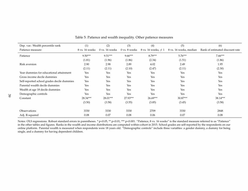
Table 5: Patience and wealth inequality. Other patience measures

Dep. var.: Wealth percentile rank (1) (2) (3) (4) (5) (6)Patience measure: 8 vs. 16 weeks 0 vs. 16 weeks 0 vs. 8 weeks 8 vs. 16 weeks, 6= 1 8 vs. 16 weeks, median Rank of estimated discount rate

Patience 9.50*** 9.51*** 9.66*** 8.79*** 5.76*** 7.66***(1.81) (1.96) (1.86) (2.34) (1.51) (1.86)

Risk aversion 2.90 2.98 2.89 4.02 2.49 1.95(2.11) (2.11) (2.10) (2.47) (2.11) (2.30)

Year dummies for educational attainment Yes Yes Yes Yes Yes YesGross income decile dummies Yes Yes Yes Yes Yes YesSelf-reported school grades decile dummies Yes Yes Yes Yes Yes YesParental wealth decile dummies Yes Yes Yes Yes Yes YesWealth at age 18 decile dummies Yes Yes Yes Yes Yes YesDemographic controls Yes Yes Yes Yes Yes YesConstant 28.34*** 28.01*** 27.93*** 26.69*** 30.87*** 38.14***

(3.50) (3.58) (3.55) (3.85) (3.45) (3.58)

Observations 3330 3330 3330 2709 3330 2848Adj. R-squared 0.08 0.07 0.08 0.06 0.07 0.08

Notes: OLS regressions. Robust standard errors in parentheses. * p<0.05, ** p<0.01, *** p<0.001. “Patience, 8 vs. 16 weeks” is the standard measure referred to as “Patience”in the other tables and figures. Ranks in the wealth and income distributions are computed within-cohort in 2015. School grades are self-reported by the respondents on ouronline platform. Parental wealth is measured when respondents were 18 years old. “Demographic controls” include three variables: a gender dummy, a dummy for beingsingle, and a dummy for having dependent children.

39

5.3 Sensitivity to definition of wealth, observation period, and selection into the experi-

ment

Table 6 shows the results from a number of additional robustness checks. The first column in Table 6

reproduces column 8 from Table 2, i.e. the specification with the richest set of control variables included.

The dependent variable in this specification is based on net wealth ranks calculated using 2015 data. In

that analysis, we focus on the latest year in the sample because we want to characterize the association

between elicited patience and wealth for individuals who have reached a life stage where their current

income is as close to its “permanent level” as possible, and where their financial position is not dom-

inated by early life decisions such as undertaking education and entering the labor market. However,

Figure 3a showed evidence that the bivariate association between patience and wealth is stable over a

much longer period, 2001-2015. In Table 6, column 2, we re-estimate the reference model reported in

column 1 using annual observations for the entire data period 2001-2015. Consistent with the impres-

sion provided by Figure 3a, the multivariate results are robust to this change, although the parameter of

interest is slightly smaller than in the preferred specification.

The theory presented in section 2 characterizes wealth as being held in just one asset. A natural

interpretation is that it reflects net wealth, which is the wealth concept we have used in the analysis

so far. An alternative interpretation is that it reflects financial assets. In column 3 we re-estimate the

reference specification using financial assets, consisting of stocks, bonds, and deposits, as the basis for

constructing the position in the wealth distribution. Also for this outcome we find that the positive

relationship between patience and the ranking in the financial asset distribution is similar to the result

obtained in the reference specification based on net wealth.22

Column 4 adjusts tax assessed values of housing by the average ratio of market prices to tax assessed

values among traded houses of the same property class and in the same location and price range. This

is done to account for the fact that the tax assessed values may be somewhat below market values (Leth-

Petersen 2010). The estimate of the patience parameter attenuates slightly but the parameter is precisely

estimated and is within two standard deviations from the reference estimate in column 1. The wealth

data including housing and financial wealth are consistently third-party reported for an exceptionally

long period. However, they lack two components of wealth that are potentially important for assessing

wealth inequality, wealth kept in the car stock and wealth accumulated in pension accounts. Data docu-

22In agreement with the results presented in Figure 3a, the more patient respondents are consistently ranked higher in thefinancial asset distribution relative to their less patient peers over the period 2001-2015 (not reported).

40

menting these two components has recently become available, but only from 2014 onwards. In column

5, we include the value of the car stock among assets and calculate the net wealth rank based on 2015

data. The patience parameter is close to the estimate in column 4.

41

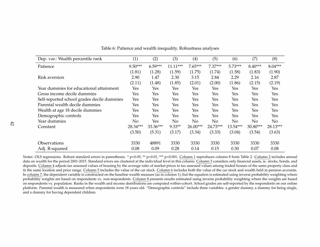
Table 6: Patience and wealth inequality. Robustness analyses

Dep. var.: Wealth percentile rank (1) (2) (3) (4) (5) (6) (7) (8)

Patience 9.50*** 6.59*** 11.11*** 7.65*** 7.37*** 5.73*** 8.40*** 8.04***(1.81) (1.28) (1.59) (1.75) (1.74) (1.58) (1.83) (1.90)

Risk aversion 2.90 1.47 2.30 3.15 2.84 2.29 2.16 2.87(2.11) (1.48) (1.85) (2.01) (2.00) (1.86) (2.15) (2.19)

Year dummies for educational attainment Yes Yes Yes Yes Yes Yes Yes YesGross income decile dummies Yes Yes Yes Yes Yes Yes Yes YesSelf-reported school grades decile dummies Yes Yes Yes Yes Yes Yes Yes YesParental wealth decile dummies Yes Yes Yes Yes Yes Yes Yes YesWealth at age 18 decile dummies Yes Yes Yes Yes Yes Yes Yes YesDemographic controls Yes Yes Yes Yes Yes Yes Yes YesYear dummies No Yes No No No No No NoConstant 28.34*** 33.36*** 9.33** 26.00*** 24.73*** 13.54*** 30.80*** 28.13***

(3.50) (5.31) (3.17) (3.34) (3.33) (3.04) (3.54) (3.63)

Observations 3330 48891 3330 3330 3330 3330 3330 3330Adj. R-squared 0.08 0.09 0.28 0.14 0.15 0.30 0.07 0.08

Notes: OLS regressions. Robust standard errors in parentheses. * p<0.05, ** p<0.01, *** p<0.001. Column 1 reproduces column 8 form Table 2. Column 2 includes annualdata on wealth for the period 2001-2015. Standard errors are clustered at the individual level in this column. Column 3 considers only financial assets, ie. stocks, bonds, anddeposits. Column 4 adjusts tax assessed values of housing by the average ratio of market prices to tax assessed values among traded houses of the same property class andin the same location and price range. Column 5 includes the value of the car stock. Column 6 includes both the value of the car stock and wealth held in pension accounts.In column 7, the dependent variable is constructed on the baseline wealth measure (as in column 1), but the equation is estimated using inverse probability weighting whereprobability weights are based on respondents vs. non-respondents. Column 8 presents results estimated using inverse probability weighting where the weights are basedon respondents vs. population. Ranks in the wealth and income distributions are computed within-cohort. School grades are self-reported by the respondents on our onlineplatform. Parental wealth is measured when respondents were 18 years old. “Demographic controls” include three variables: a gender dummy, a dummy for being single,and a dummy for having dependent children.

42

We further include wealth kept in pension accounts in column 6. This addition slightly mutes the

point estimate of the patience parameter. There are good reasons why adding pension wealth would

attenuate the estimate. 90 percent of contributions to pension accounts are made to illiquid employer

organized pension accounts (Kreiner et al. 2017), and the contributions are predominantly determined by

collective labor market agreements. As Chetty et al. (2014a) document, the majority responds passively

to these savings mandates, i.e. they do not adjust other types of savings in response to these savings

mandates.

Only a fraction of the subjects whom we invited to participate in the experiment accepted the invita-

tion, and this can potentially imply that our sample is selected and not representative of the population

at large. In column 7 we re-estimate the reference specification from column 1 using propensity score

weighting, where the propensity scores measure the propensity to participate in the experiment for all

the subjects who were invited. The propensity scores are estimated using variables created from infor-

mation available in the administrative registries accessible for both participants and non-participants:

year dummies for educational attainment, decile dummies for income, parental wealth, and wealth at

age 18 as well as age dummies, a gender dummy, a dummy for being single, and a dummy for having

dependent children. The results presented in column 7 are close to the estimate from the reference spec-

ification. In Column 8 we construct propensity scores measuring the propensity to be in the experiment

compared to the population at large. As with previous cases, we find no important deviations from the

benchmark model. The propensity score weighting approach is based on the assumption that the selec-

tion into the experiment can be adequately captured by the set of covariates on which the propensity

score is estimated. To the extent that this is a reasonable assumption, our results do not appear too spe-

cific to the sample for which we elicit patience measures. In total, Table 6 presents a series of alternative

estimates designed in order to check the validity of our main finding showing that elicited patience is

associated with wealth inequality and that the magnitude of the association is non-trivial.

6 Concluding remarks

According to standard life-cycle savings theory, differences in how much people discount the future

generate differences in savings behavior and thereby wealth inequality. Data limitations previously

prevented the examination of a direct link between empirical time discounting measures and wealth

inequality operating through the savings channel. We address this problem by analyzing a unique com-

43

bination of data with information about individuals’ time discounting and real-world wealth for a large

sample of middle-aged individuals in Denmark. Subjective measures of patience are elicited using stan-

dard experimental methods and linked to longitudinal administrative wealth records for a period cov-

ering 15 years.

Our measures of time discounting indicate substantial heterogeneity in individuals’ patience, and we

show that individuals with a high level of patience are systematically positioned higher in the wealth

distribution in each year over the 15 year period for which we have individual wealth data compared to

those who have low levels of patience. The association between patience and the position in the wealth

distribution is robust and significant for all our measures of time discounting, of the same magnitude

as the correlation between education and wealth and, on average, roughly half as large as the influence

of parental wealth on the wealth rank. The association also exists after controlling for education, risk

aversion, income, initial wealth and parental wealth, suggesting that the savings mechanism is impor-

tant. Moreover, we replicate the significant association between discounting and wealth position in an

independent data set in which the patience measure – collected in the early 1970s – predicts differences

in individuals’ wealth 30 years later.

We also find that people with a relatively low level of patience are more likely to be persistently af-

fected by liquidity constraints. This is consistent with models where impatient people run down their

assets in order to keep current spending relatively high, implying that they face a higher risk of be-

coming credit constrained (Krueger et al., 2016; Carroll et al., 2017). In this sense, liquidity constraints

are to some extent self-imposed as described in these models. In addition, individuals who are persis-

tently affected by liquidity constraints have limited opportunities to further reduce their wealth levels

through the borrowing/savings channel. This implies that the variation of patience levels among the

subset of individuals who are persistently affected by credit constraints is predicted to mute the rela-

tionship between patience and the wealth rank – a prediction that is nicely borne out by the data. In

contrast, if we limit our analysis to the subset of individuals who are not credit constrained (i.e., where

the savings/borrowing channel is “fully operative”), we find that the influence of differences in time

discounting is roughly 50% higher than in the overall sample.

Thus, taken together, our results suggest that differences in individuals’ time discounting play a sig-

nificant role for their wealth rank and they point, more generally, to the potential importance of incorpo-

rating heterogeneous time discounting into models of consumption and savings behavior as originally

suggested by Krusell and Smith (1998) and recently applied by Hubmer et al. (2016), Krueger et al. (2016),

44

Carroll et al. (2017), De Nardi and Fella (2017) and Alan et al. (2017).

Our results indicate that the elicited patience measures contain important and relevant information

about the order of subjects’ evaluations of intertemporal trade-offs that are predictive of subjects’ wealth

position. Therefore, making a direct link between experimentally elicited discounting behavior and the

discount rates entering models of aggregate savings behavior would appear to be a natural next step.

However, taking this step is likely to be a challenge in practice. As is well-known in the experimental

literature (Frederick et al. 2002), discount rates elicited under relatively small stakes are typically much

larger than discount rates that are implied by aggregate models of discounting. However, insofar as the

ordering of patience derived from small stake choice tasks is the same as it would be in a setting with

large stakes, the experiments can credibly elicit the ordering of individuals in terms of their discounting

behavior, as done in our analyses.

This paper provides a positive analysis of the relationship between discounting behavior and wealth

inequality. The normative consequences of the results are, however, not obvious although effects of dis-

count rate heterogeneity may have implications for macroeconomic policies and policies that provide

insurance against shocks. Our results suggest that households with high discount rates are more likely

to face liquidity constraints such that they are less able to smooth consumption over the business cycle.

Thus, business cycle shocks may impose asymmetric costs on households with high and low discount

rates and the costs of business cycles may be larger in the presence of discount rate heterogeneity. There-

fore, the existence of discount rate heterogeneity and its effects on wealth may have a bearing on the

desirability and the effectiveness of macroeconomic policies, the design of insurance institutions, and

policies that aim at increasing the savings of poor households.

45

Appendices

A Theory

A.1 Derivation of equation (3)

The solution to the maximization problem is characterized by the standard Euler equation/Keynes-

Ramsey rulec (a)c (a)

=r− ρ

θ, (5)

and the transversality condition w (T) = 0. By integrating the flow budget constraint (2), we obtain the

following intertemporal budget constraint

w (a) = era[

w (0) +ˆ a

0y (τ) e−rτdτ −

ˆ a

0c (τ) e−rτdτ

]. (6)

By evaluating (6) at a = T and using w (T) = 0 in the optimum, we obtain

Y ≡ w (0) +ˆ T

0y (τ) e−rτdτ =

ˆ T

0c (τ) e−rτdτ.

By integrating (5), we obtain

c (a) = c (0) er−ρ

θ a, (7)

which is substituted into the above equation in order to get

Y (0) = c (0)ˆ T

0e

r(1−θ)−ρθ τdτ.

By solving the integral and isolating c (0), we obtain

c (0) = Y (0)ρ + r (θ − 1)

θ(

1− er(1−θ)−ρ

θ T) . (8)

Next, we substitute equation (7) into (6), which gives

w (a) = era[

w (0) +ˆ a

0y (τ) e−rτdτ − c (0)

θ

r (1− θ)− ρ

(e

r(1−θ)−ρθ a − 1

)],

46

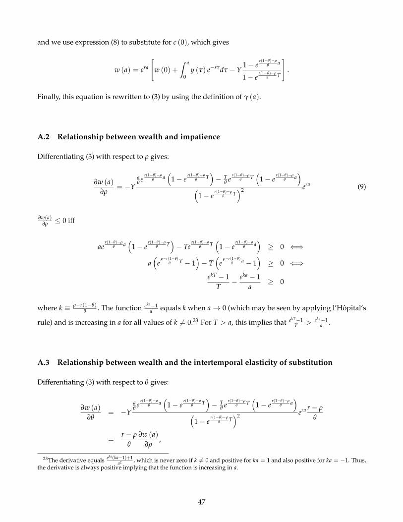
and we use expression (8) to substitute for c (0), which gives

w (a) = era

[w (0) +

ˆ a

0y (τ) e−rτdτ −Y

1− er(1−θ)−ρ

θ a

1− er(1−θ)−ρ

θ T

].

Finally, this equation is rewritten to (3) by using the definition of γ (a).

A.2 Relationship between wealth and impatience

Differentiating (3) with respect to ρ gives:

∂w (a)∂ρ

= −Yaθ e

r(1−θ)−ρθ a

(1− e

r(1−θ)−ρθ T

)− T

θ er(1−θ)−ρ

θ T(

1− er(1−θ)−ρ

θ a)

(1− e

r(1−θ)−ρθ T

)2 era (9)

∂w(a)∂ρ ≤ 0 iff

aer(1−θ)−ρ

θ a(

1− er(1−θ)−ρ

θ T)− Te

r(1−θ)−ρθ T

(1− e

r(1−θ)−ρθ a

)≥ 0 ⇐⇒

a(

eρ−r(1−θ)

θ T − 1)− T

(e

ρ−r(1−θ)θ a − 1

)≥ 0 ⇐⇒

ekT − 1T

− eka − 1a

≥ 0

where k ≡ ρ−r(1−θ)θ . The function eka−1

a equals k when a→ 0 (which may be seen by applying l’Hôpital’s

rule) and is increasing in a for all values of k 6= 0.23 For T > a, this implies that ekT−1T > eka−1

a .

A.3 Relationship between wealth and the intertemporal elasticity of substitution

Differentiating (3) with respect to θ gives:

∂w (a)∂θ

= −Yaθ e

r(1−θ)−ρθ a

(1− e

r(1−θ)−ρθ T

)− T

θ er(1−θ)−ρ

θ T(

1− er(1−θ)−ρ

θ a)

(1− e

r(1−θ)−ρθ T

)2 era r− ρ

θ

=r− ρ

θ

∂w (a)∂ρ

,

23The derivative equals eka(ka−1)+1a2 , which is never zero if k 6= 0 and positive for ka = 1 and also positive for ka = −1. Thus,

the derivative is always positive implying that the function is increasing in a.

47

where the last equality comes from equation (9). We know from Appendix A.2 that ∂wa/∂ρ ≤ 0. Hence,

∂wa/∂θ ≤ 0 if r > ρ, ∂wa/∂θ ≥ 0 if r < ρ and ∂wa/∂θ = 0 if r = ρ. QED.

48

B Experiment

B.1 Invitation letter

Figure A1: Invitation letter

49

English translation of the invitation letter:

Dear «name»,

University of Copenhagen invites you to participate in a study on the Internet. The study is part of aresearch project about understanding the basis for the Danes’ financial decisions. We already know a lotmore about people’s personal financial decisions than we did before the financial crisis, but there is stillmuch we need to understand - and that is why we are asking for your help.

It takes about 30-50 minutes to complete the study. When you are finished, you will typically receiveprize money and it will be automatically transferred to your NemKonto. The amount depends, i.a., onthe choices that you make during the study and will on average correspond to a decent hourly wage.

The study is conducted on the Internet. You will consider questions concerning savings and invest-ments, among other things. The rules will be explained once you have logged in. The study is open forparticipation through «date».

The Data Protection Agency has approved the research project, which means that our procedurescomply with the Act on Processing of Personal Data. An important part of the Data Protection Agency’srequirements is that your answers will be treated anonymously. To ensure anonymity, we have formeda random username for you. To participate, please log in at the following website: analyse.econ.ku.dk.

Username: «username» Password: «password»

The invitation is personal and we therefore ask you not to pass on username and password to others.Please feel free to contact us if you are having trouble logging in or have any further questions. You cancall project coordinator Gregers Nytoft Rasmussen at phone number 35 33 02 77 Monday-Thursday 2:00p.m. – 5:30 p.m. or write to the address analyse@econ.ku.dk.

Sincerely yours,

Søren Leth-Petersen

Project manager, professor

50

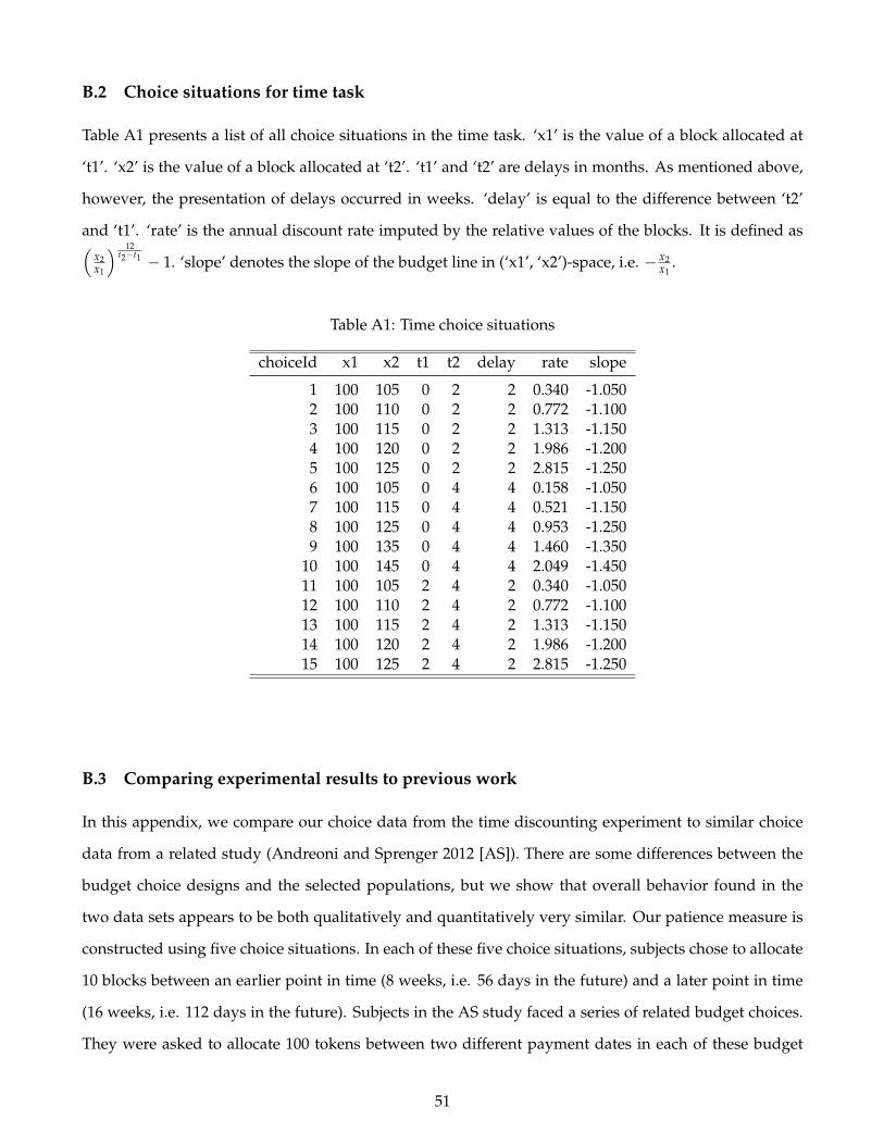
B.2 Choice situations for time task

Table A1 presents a list of all choice situations in the time task. ‘x1’ is the value of a block allocated at

‘t1’. ‘x2’ is the value of a block allocated at ‘t2’. ‘t1’ and ‘t2’ are delays in months. As mentioned above,

however, the presentation of delays occurred in weeks. ‘delay’ is equal to the difference between ‘t2’

and ‘t1’. ‘rate’ is the annual discount rate imputed by the relative values of the blocks. It is defined as(x2x1

) 12t2−t1 − 1. ‘slope’ denotes the slope of the budget line in (‘x1’, ‘x2’)-space, i.e. − x2

x1.

Table A1: Time choice situations

choiceId x1 x2 t1 t2 delay rate slope

1 100 105 0 2 2 0.340 -1.0502 100 110 0 2 2 0.772 -1.1003 100 115 0 2 2 1.313 -1.1504 100 120 0 2 2 1.986 -1.2005 100 125 0 2 2 2.815 -1.2506 100 105 0 4 4 0.158 -1.0507 100 115 0 4 4 0.521 -1.1508 100 125 0 4 4 0.953 -1.2509 100 135 0 4 4 1.460 -1.350

10 100 145 0 4 4 2.049 -1.45011 100 105 2 4 2 0.340 -1.05012 100 110 2 4 2 0.772 -1.10013 100 115 2 4 2 1.313 -1.15014 100 120 2 4 2 1.986 -1.20015 100 125 2 4 2 2.815 -1.250

B.3 Comparing experimental results to previous work

In this appendix, we compare our choice data from the time discounting experiment to similar choice

data from a related study (Andreoni and Sprenger 2012 [AS]). There are some differences between the

budget choice designs and the selected populations, but we show that overall behavior found in the

two data sets appears to be both qualitatively and quantitatively very similar. Our patience measure is

constructed using five choice situations. In each of these five choice situations, subjects chose to allocate

10 blocks between an earlier point in time (8 weeks, i.e. 56 days in the future) and a later point in time

(16 weeks, i.e. 112 days in the future). Subjects in the AS study faced a series of related budget choices.

They were asked to allocate 100 tokens between two different payment dates in each of these budget

51

choices. For comparability, we pick the most similar delays in their experiment, namely 35 and 70 days.

In addition to different delays and different number of blocks/tokens to allocate, the two studies vary

with respect to the subject sample and the presentation format. Specifically, the AS sample consists of

97 San Diego undergraduates, whereas our study uses data from 3,620 middle-aged individuals from

the general Danish population. In their experiment, subjects were presented an ordered list of allocation

choices with fixed payment dates on each screen. In contrast, we displayed each allocation choice in

our study separately on a new screen. The five allocation choices we use to construct our index were

interleaved with other choices involving different payment dates, and they appeared in randomized

order. Furthermore, we held the value of an earlier block fixed at 100 points, whereas AS fixed the price

of a future token for each date configuration.

Figure A2 juxtaposes the average share of blocks/tokens that subjects postponed to the later date

as a function of the relative gain measured in percent from delaying it. In both experiments, it is as

expected that the higher the compensation (‘gain of postponing’), the more the subjects are willing to

postpone gratification. Importantly, the average behavior found in the the two data sets appears to be

both qualitatively and quantitatively very similar.

52

Figure A2: Comparing choices in experiment to existing work

0.0

0.2

0.4

0.6

0.8

1.0

gain of postponing in percent

mea

n sh

are

of b

lock

s/to

kens

pos

tpon

ed

Andreoni and Sprenger (2012)present study

0 5 10 15 20 25 30 35 40 45 50

Notes: The figure shows the average share of blocks/tokens postponed to the later date by the subjects as a function of therelative gain measured in percent from delaying it. For our data, the gain is calculated as the value of a later block in pointsmeasured in percent of the point value of a sooner block. For Andreoni and Sprenger (2012) the gain is calculated as the priceof a later token in percent of the price of a sooner token.

B.4 Risk task and risk aversion measure

Risk task: We use investment games (IGs) similar to Gneezy and Potters (1997) to measure risk aversion.

The main differences to their setup are: (i) that we used a graphical interface to present the investment

choice, and (ii) that we varied both probabilities of winning and rates of return across the choice situa-

tions. A typical choice situation is depicted in Figure A3. The left panel shows the initial state of a choice

situation. The subject was endowed with ten 100-point blocks positioned at the very left of the screen

and could then decide how many of these blocks to invest in a risky asset. The (binary) risky asset, de-

picted on the right-hand side of the choice screen, resulted in either a good outcome or a bad outcome.

In the example, the good outcome occurred with probability 60% (illustrated by the wheel on top of the

risky asset) and yielded 130 points for each invested 100-point block. The bad outcome occurred with

probability 40% and yielded 70 points for each invested 100-point block. The user interface worked in

53

the same way as in the time task.

Figure A3: Risk choice task. Initial screen (a) and selected option (b)

(a)

100 70 130

100 70 130

100 70 130

100 70 130

100 70 130

100 70 130

100 70 130

100 70 130

100 70 130

100 70 130

40%60%invest less -

invest more +

Confirm

(b)

in 40 of 100 cases you receive a total

of 760

in 60 of 100 casesyou receive a total

of 1240

100 70 130

100 70 130

you keep 200 you invest 800 you receive 560 you receive 1040

100 70 130

100 70 130

100 70 130

100 70 130

100 70 130

100 70 130

100 70 130

100 70 130

40%60%invest less -

invest more +

Confirm

A total of 15 choice situations were implemented. They varied in terms of probabilities and rates of

return. Table A2 presents a list of all choice situations in the risk task. ‘vb’ is the value of a block. ‘m1’

is the multiplier in case the good state occurs, in which case the new value of a block is vb*m1. ‘m2’

is the multiplier in case the bad state occurs, in which case the new value of a block is vb*m2. ‘p’ is

the probability of the good state. ‘mev’ is the expected multiplier, mev = p×m1 + (1− p)×m2. ‘msd’

standard deviation of the multiplier, msd =√

p× (m1 −mev)2 + (1− p)× (m2 −mev)2. ‘mskew’ is the

skewness of the multiplier, mskew = p×(m1−mev)3+(1−p)×(m2−mev)3

msd3 . ‘slope’ is the slope of the budgets, i.e.

the ratio of prices, slope = m2−1m1−1 .

Like in the other tasks, choice situations in the risk task appeared in individualized random order. If

the random choice situation picked in the payment stage was a risky choice situation, the subject was

again confronted with her choice. The choice could not be reverted at this stage, however. The subject

was then asked to resolve uncertainty in the present situation. This was done by spinning the wheel on

top of the risky asset. The final payout corresponded to the sum of the safe account and the resolved

outcome of the originally risky account. Payments were transferred directly to subjects’ NemKonto on

the next banking day.

Risk aversion measure: We construct a risk aversion index as follows: We take all choice situations with

zero skewness, i.e. with probability 0.5 (choiceId 1, 4, 7, 14 and 15 in Table A2). We then normalize and

54

Table A2: Risk choice situations

choiceId vb m1 m2 p mev msd mskew slope1 100 1.21 0.81 0.5 1.010 0.200 0.000 -0.9052 100 1.41 0.91 0.2 1.010 0.200 1.500 -0.2203 100 1.11 0.61 0.8 1.010 0.200 -1.500 -3.5454 100 1.31 0.71 0.5 1.010 0.300 0.000 -0.9355 100 1.61 0.86 0.2 1.010 0.300 1.500 -0.2306 100 1.16 0.41 0.8 1.010 0.300 -1.500 -3.6887 100 1.35 0.75 0.5 1.050 0.300 0.000 -0.7148 100 1.65 0.90 0.2 1.050 0.300 1.500 -0.1549 100 1.20 0.45 0.8 1.050 0.300 -1.500 -2.750

10 100 1.50 0.40 0.6 1.060 0.539 -0.408 -1.20011 100 1.72 0.62 0.4 1.060 0.539 0.408 -0.52812 100 1.45 0.35 0.6 1.010 0.539 -0.408 -1.44413 100 1.67 0.57 0.4 1.010 0.539 0.408 -0.64214 100 1.51 0.50 0.5 1.005 0.505 0.000 -0.98015 100 1.61 0.60 0.5 1.105 0.505 0.000 -0.656

aggregate using the mean.24 We define:

φrisk aversion = mean( z1

10, ...,

z5

10

),

where zi denotes the number of blocks kept in the safe account in choice situation i. φrisk aversion is an

index of risk aversion with φrisk aversion ∈ [0, 1]. Higher values of φrisk aversion indicate greater risk aversion

and a φrisk aversion of zero indicates minimum risk aversion (or, more precisely, a degree of risk aversion

below the one implied by z = 1 in all situations).

C Empirical results

C.1 Main result for subjects with both parents still alive

In this section, we document that the parameter on patience is robust to including only observations for

individuals where both parents are still alive. Table A3, column 1 repeats Table 2, column 5, and Table A3,

column 2 performs the corresponding estimation but on the subset of observations where respondents’

parents are both still alive. As is seen from the table, the results are for all practical purposes similar, and

we take this as an indication that inheritance does not drive the correlation between the wealth rank and

our patience measure.

24Using the median does not change our results.

55

Table A3: Patience and wealth inequality. For a subsample of individuals with both parents alive

Dep. var.: Wealth percentile rank (1) (2)

Patience 9.33*** 8.05***(1.80) (2.28)

Year dummies for educational attainment Yes YesGross income decile dummies Yes YesSelf-reported school grades decile dummies Yes YesParental wealth decile dummies Yes YesWealth at age 18 decile dummies No NoDemographic controls No NoConstant 33.36*** 33.67***

(2.98) (3.86)

Observations 3330 2178Adj. R-squared 0.07 0.06

Notes: OLS regressions. Robust standard errors in parentheses. * p<0.05, ** p<0.01, *** p<0.001. The measurement of patienceis described in expression (4). Ranks in the wealth and income distributions are computed within-cohort in 2015. Gross incomedoes not include capital income. School grades are self-reported by the respondents on our online platform. Parental wealth ismeasured when respondents were 18 years old.

C.2 Marginal interest rates

Here we present details about the construction of marginal interest rates. We obtained access to admin-

istrative register data from the Danish tax authority containing information on the value of loans at the

end of 2013 and 2014 for all loans that the respondents held in Denmark. In addition, the data comprise

interest payments during 2014 at the individual loan level. This allows us to approximate the interest

rate paid on each loan as ri,l =R14

i,l12 (D13

i,l +D14i,l )

, where R14i,l is the sum of interest payments on loan l for indi-

vidual i during 2014, D13i,l is the value of the loan at the end of 2013, and D14

i,l is the value of the loan at

the end of 2014. We only include non-mortgage loans and require a minimum denominator in the above

equation of 1,000 DKK. The resulting interest rates are censored at the 5th and the 95th percentiles. Our

approximation of the interest rate is exact if the debt evolves linearly between 2013 and 2014. If it does

not, the computation of the interest rate may introduce a measurement error.

For respondents with loan accounts, we define the marginal interest rate as the highest calculated

loan account-specific interest rate. If a respondent only has deposit accounts, we define the marginal

interest rate as the smallest account-specific interest rate among the calculated account-specific interest

rates for that respondent. The rationale is that the cost of liquidity is given by the loan account with

56

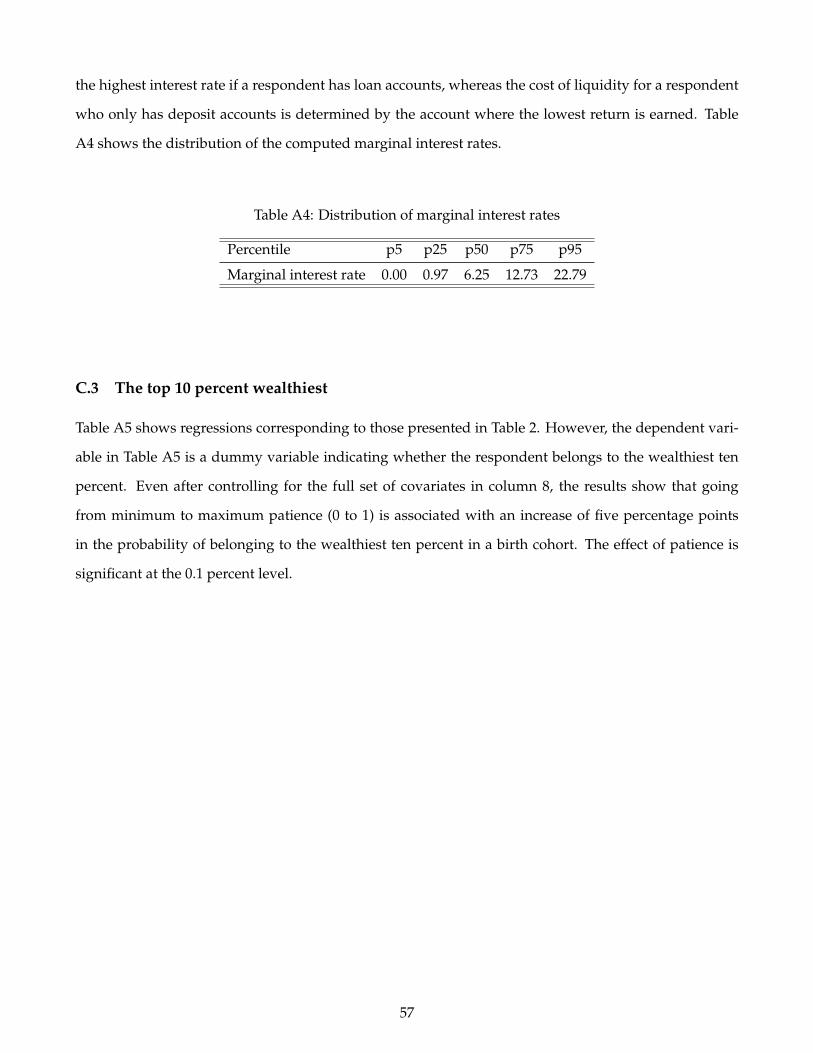
the highest interest rate if a respondent has loan accounts, whereas the cost of liquidity for a respondent

who only has deposit accounts is determined by the account where the lowest return is earned. Table

A4 shows the distribution of the computed marginal interest rates.

Table A4: Distribution of marginal interest rates

Percentile p5 p25 p50 p75 p95

Marginal interest rate 0.00 0.97 6.25 12.73 22.79

C.3 The top 10 percent wealthiest

Table A5 shows regressions corresponding to those presented in Table 2. However, the dependent vari-

able in Table A5 is a dummy variable indicating whether the respondent belongs to the wealthiest ten

percent. Even after controlling for the full set of covariates in column 8, the results show that going

from minimum to maximum patience (0 to 1) is associated with an increase of five percentage points

in the probability of belonging to the wealthiest ten percent in a birth cohort. The effect of patience is

significant at the 0.1 percent level.

57

Table A5: Top 10% wealthiest

Dep. var.: Dummy for top 10% of the wealth distribution (1) (2) (3) (4) (5) (6) (7) (8)

Patience 0.09*** 0.07*** 0.06*** 0.06*** 0.06** 0.05** 0.05** 0.05**(0.02) (0.02) (0.02) (0.02) (0.02) (0.02) (0.02) (0.02)

Risk aversion 0.01 0.01(0.02) (0.02)

Year dummies for educational attainment No Yes Yes Yes Yes Yes Yes YesGross income decile dummies No No Yes Yes Yes Yes Yes YesSelf-reported school grades decile dummies No No No Yes Yes Yes Yes YesParental wealth decile dummies No No No No Yes Yes Yes YesWealth at age 18 decile dummies No No No No No Yes Yes YesDemographic controls No No No No No No No YesConstant 0.04*** -0.02 -0.02 -0.01 -0.02 -0.05* -0.06* -0.06*

(0.01) (0.01) (0.02) (0.02) (0.03) (0.03) (0.03) (0.03)

Observations 3620 3620 3620 3330 3330 3330 3330 3330Adj. R-squared 0.01 0.03 0.05 0.05 0.07 0.09 0.09 0.09

Notes: OLS regressions. Dep. var.: Dummy for top 10% of the within-cohort wealth distribution, 2015. Robust standard errors in parentheses. * p<0.05, ** p<0.01, ***p<0.001. Ranks in the wealth and income distributions are computed within-cohort. Gross income does not include capital income. School grades are self-reported by therespondents on our online platform. Parental wealth is measured when respondents were 18 years old. “Demographic controls” include three variables: a gender dummy, adummy for being single, and a dummy for having dependent children. The number of observations decreases in columns 4-8 due to some of the respondents not reportingschool grades.

58

C.4 Comparing patience measured in the DLSY survey and in the experiment

In this appendix, we compare patience elicited with the DLSY survey questions to the patience elicited

in the experiment. We do this with data from a large-scale online study conducted during the year 2018.

4,152 Danes of the cohorts with birth year 1967 to 1986 completed the study. In addition to the DLSY

survey measure described in section 5.1, the study also included an experimental time task with real

monetary incentives. With the exception that there were 100 blocks instead of 10 to be allocated between

two points in time in each of the choice situations, the time task was identical to that described in section

3. For comparability, we bin the 100 blocks into 10, and then construct our patience index based on the

t1 = 2 months vs. t2 = 4 months allocations.

Figure A4 depicts the arithmetic means (dots) of our patience index conditional on the three possible

responses in the DLSY question, and 95% confidence intervals (whiskers). It shows that responses in the

DLSY question and choices in the real-incentivized, experimental time task are highly and significantly

correlated.

Figure A4: Comparison of DLSY and experimental measure

●

●

●

0.60

0.65

0.70

impatient middle patient

Preferred income profile (DLSY question)

Pat

ienc

e in

dex

(exp

erim

enta

l mea

sure

)

C.5 Structural estimation of patience

In this appendix, we describe the structural estimation of patience used in the sensitivity analysis in

section 5.2. Consider the decision problem from the subject’s perspective. Define a choice situation S

59

(see rows in Table A1) as a tuple of attributes (x1, t1, x2, t2), where x1 and x2 denote the value (points) of

a block materializing at the earlier point in time t1 and the later point in time t2, respectively. Delays will

be reported in months.

Assuming additively separable time discounting, a subject’s choice z is the outcome of the maximiza-

tion problem

maxz∈{0,1,...,10}

d(t1)u(w1) + d(t2)u(w2) ,

subject to the budget constraint

w2 = − x2

x1(w1 − 10x1) ,

where w1 = (10− z)x1 and w2 = z · x2 denote the total number of points allocated to t1 and t2, respec-

tively. Therefore, z ∈ {0, 1, ..., 10} indicates the number of blocks saved to the later point in time. In our

setup, it holds that x1 = 100 points in every choice situation. The slope of the budget lines is thus given

by − x2100 .

To be able to compare estimated discount rates with our nonparametric index of patience, we first

restrict attention to choice situations with payment dates t1 = 2 months and t2 = 4 months. In order to

make the model operational, we have to assume specific functional forms for the discount function d(t)

and the utility function u(w). Assuming continuous compounding, d (t) is specified as

d(t) = e−ρ t12 ,

where ρ is the annualized discount rate. We further assume that utility is linear in outcomes, i.e. u(w) =

w. Since, for all choice situations, it holds that x1 < x2, discount rates are bounded from below at zero.

Note that a single choice situation S only informs us about whether an individual is more or less patient

than a certain threshold (see the rates listed in Table A1). The fact that we observe multiple choices

per subject and that these choice situations vary with respect to their implicit interest rates permit us to

bound the discount rate to an interval.

Until now, we have considered a deterministic model. To incorporate the possibility of errors, we

have to make an assumption about the stochastic nature of choices. To do this, we assume random

utility with additively separable choice noise (McFadden 1974, 1981). Denoting Sz as the temporal points

60

allocation arising from choice z in a specific situation, the utility of Sz is given by U(Sz) = d(t1)u((10−

z)x1) + d(t2)u(z · x2). We presume that the utility of a temporal stream of outcomes equals V(z) =

U(Sz) + εz, with εz being an i.i.d. random variable representing error in evaluating utility.

Under the assumption that εz follows a Type I extreme value distribution with (inverse) scale (preci-

sion) parameter λ, and z′ 6= z, an individual chooses allocation z if V(z) > V(z′). This yields the choice

probability Prob(·) of allocation z:

Prob(z) = Prob(U(Sz)−U(Sz′) > εz′ − εz)) =eλU(Sz)

∑10k=0 eλU(Sk)

.

We estimate the model using maximum likelihood. The objective function to be maximized is equal to

f (S ; θ) =m

∏j=1

10

∏k=0

Prob(z)1[Sz=Sk ] ,

where θ denotes the vector of parameters to be estimated, the first product multiplies over all m choice

situations in S , and the second product multiplies over all eleven possible allocations. Note that the

stochastic specification of the model introduces an additional precision parameter λ, which is con-

strained to be positive. λ = 0 represents random choice. In this case, choice probabilities follow a

uniform distribution over the eleven possible allocations. Large λ’s, on the other hand, indicate higher

precision.

We report results for 3,087 subjects for whom we were able to obtain parameter estimates. Figure A5

depicts the distribution of estimated discount rates. It includes subjects who always chose to keep or save

all blocks in all choice situations. For these subjects, we set the actual discount rate to the maximum and

minimum possible discount rate, respectively. The mean of the estimated discount rates in the sample

is 0.52 per annum. Table 5 shows that we obtain similar results when we use the rank of the estimated

discount rates instead of the the patience index as a right-hand side variable in the wealth regressions.

We have also estimated a version of the structural model where we use a CRRA subutility function

u(w) and included the concavity parameter among the estimated parameters. This exercise resulted in

discount rates very similar to those reported here, and with more or less the same association between

patience and wealth as reported in Table 5.

61

Figure A5: Distribution of structurally estimated discount rates

0

5

10

15

20

25

30

35

40

45

Per

cent

0 .1 .2 .3 .4 .5 .6 .7 .8 .9 1 1.1 1.2 1.3 1.4Estimated discount rate (rho)

Notes: 3,087 observations. Mean = 0.52.

62

References

Abdellaoui, M., Attema, A. E., and Bleichrodt, H. (2010). Intertemporal tradeoffs for gains and losses:An experimental measurement of discounted utility. Economic Journal, 120(545):845–866.

Abdellaoui, M., Bleichrodt, H., and L’Haridon, O. (2013). Sign-dependence in intertemporal choice.Journal of Risk and Uncertainty, 47(3):225–253.

Adermon, A., Lindahl, M., and Waldenström, D. (2018). Intergenerational wealth mobility and the roleof inheritance: Evidence from multiple generations. Economic Journal, forthcoming.

Alan, S., Browning, M., and Ejrnæs, M. (2017). Income and consumption: A semi structural analysis ofpervasive heterogeneity. Forthcoming in Journal of Political Economy.

Anderhub, V., Gäuth, W., Mäuller, W., and Strobel, M. (2000). An experimental analysis of intertemporalallocation behavior. Experimental Economics, 3(2):137–152.

Andersson, O., Holm, H. J., Tyran, J.-R., and Wengström, E. (2016). Risk aversion relates to cognitiveability: Preferences or noise? Journal of the European Economic Association, 14(5):1129–1154.

Andreoni, J. and Sprenger, C. (2012). Estimating time preferences from convex budgets. American Eco-nomic Review, 102(7):3333–3356.

Attema, A. E., Bleichrodt, H., Gao, Y., Huang, Z., and Wakker, P. P. (2016). Measuring discountingwithout measuring utility. American Economic Review, 106(6):1476–1494.

Attema, A. E., Bleichrodt, H., Rohde, K. I., and Wakker, P. P. (2010). Time-tradeoff sequences for analyz-ing discounting and time inconsistency. Management Science, 56(11):2015–2030.

Augenblick, N., Niederle, M., and Sprenger, C. (2015). Working over time: Dynamic inconsistency inreal effort tasks. Quarterly Journal of Economics, 130(3):1067–115.

Backes-Gellner, U., Herz, H., Kosfeld, M., and Oswald, Y. (2017). The role of economic time preferencesin human capital acquisition and labor market transition. Technical report, Working paper.

Barberis, N., Huang, M., and Thaler, R. H. (2006). Individual preferences, monetary gambles, and stockmarket participation: A case for narrow framing. American Economic Review, 96(4):1069–1090.

Barsky, R. B., Juster, F. T., Kimball, M. S., and Shapiro, M. D. (1997). Preference parameters and behavioralheterogeneity: An experimental approach in the health and retirement study. Quarterly Journal ofEconomics, 112(2):537–579.

Benartzi, S. and Thaler, R. H. (1995). Myopic loss aversion and the equity premium puzzle. QuarterlyJournal of Economics, 110(1):73–92.

63

Blinder, A. S. and Weiss, Y. (1976). Human capital and labor supply: A synthesis. Journal of PoliticalEconomy, 84(3):449–472.

Boserup, S., Kopczuk, W., and Kreiner, C. (2018). Born with a silver spoon? Danish evidence on wealthinequality in childhood. Economic Journal.

Boserup, S. H., Kopczuk, W., and Kreiner, C. T. (2016). The role of bequests in shaping wealth inequality:Evidence from Danish wealth records. American Economic Review: Papers and Proceedings, 106(5):656–61.

Card, D., Chetty, R., Feldstein, M. S., and Saez, E. (2010). Expanding access to administrative data forresearch in the United States. Technical report, White paper for the initiative "Future Research in theSocial, Behavioral & Economic Sciences", U.S. National Science Foundation.

Carroll, C., Slacalek, J., Tokuoka, K., and White, M. N. (2017). The distribution of wealth and the marginalpropensity to consume. Quantitative Economics, forthcoming.

Carroll, C. D., Slacalek, J., and Tokuoka, K. (2014). The distribution of wealth and the MPC: Implicationsof new European data. American Economic Review: Papers and Proceedings, 104(5):107–111.

Carvalho, L., Meier, S., and Wang, S. (2016). Poverty and economic decision-making: Evidence fromchanges in financial resources at payday. American Economic Review, 106(2):260–284.

Chabris, C. F., Laibson, D., Morris, C. L., Schuldt, J. P., and Taubinsky, D. (2008). Individual laboratory-measured discount rates predict field behavior. Journal of risk and uncertainty, 37(2-3):237.

Charles, K. K. and Hurst, E. (2003). The correlation of wealth across generations. Journal of PoliticalEconomy, 111:1155–1182.

Chetty, R., Friedman, J. N., Leth-Petersen, S., Nielsen, T. H., and Olsen, T. (2014a). Active vs. passivedecisions and crowd-out in retirement savings accounts: Evidence from Denmark. Quarterly Journal ofEconomics, 129(3):1141–1219.

Chetty, R., Hendren, N., Kline, P., and Saez, E. (2014b). Where is the land of opportunity? The geographyof intergenerational mobility in the United States. Quarterly Journal of Economics, 129(4):1553–1623.

Cicchetti, C. J. and Dubin, J. A. (1994). A microeconometric analysis of risk aversion and the decision toself-insure. Journal of Political Economy, 102(1):169–186.

Clark, G. and Cummins, N. (2014). Intergenerational wealth mobility in England, 1858-2012. Surnamesand social mobility. Economic Journal, 125:61–85.

Cohen, J. D., Ericson, K. M., Laibson, D., and White, J. M. (2016). Measuring time preferences. Technicalreport, NBER working paper 22455.

De Nardi, M. (2004). Wealth inequality and intergenerational links. Review of Economic Studies, 71(3):743–768.

64

De Nardi, M. and Fella, G. (2017). Saving and wealth inequality. Review of Economic Dynamics, forthcom-ing.

Dohmen, T., Falk, A., Huffman, D., and Sunde, U. (2010). Are risk aversion and impatience related tocognitive ability? American Economic Review, 100(3):1238–1260.

Eckel, C., Johnson, C., and Montmarquette, C. (2005). Saving decisions of the working poor: Short-and long-term horizons. In Harrison, G. W., Carpenter, J., and List, J. A., editors, Field Experiments inEconomics (Research in Experimental Economics, Volume 10), pages 219–260. Emerald Group PublishingLimited.

Epper, T., Fehr-Duda, H., and Bruhin, A. (2011). Viewing the future through a warped lens: Why uncer-tainty generates hyperbolic discounting. Journal of Risk and Uncertainty, 43(3):169–203.

Fagereng, A., Guiso, L., Malacrino, D., and Pistaferri, L. (2018). Heterogeneity and persistence in returnsto wealth. Nber working paper no. 22822, Working paper.

Falk, A., Becker, A., Dohmen, T., Enke, B., Huffman, D., and Sunde, U. (2018). Global evidence oneconomic preferences. Forthcoming in Quarterly Journal of Economics.

Frederick, S., Loewenstein, G., and O’Donoghue, T. (2002). Time discounting and time preference: Acritical review. Journal of Economic Literature, 40(2):351–401.

Gneezy, U. and Potters, J. (1997). An experiment on risk taking and evaluation periods. The QuarterlyJournal of Economics, 112(2):631–645.

Haider, S. and Solon, G. (2006). Life-cycle variation in the association between current and lifetimeearnings. American Economic Review, 96(4):1308–1320.

Harrison, G. W., Lau, M. I., and Williams, M. B. (2002). Estimating individual discount rates in Denmark:A field experiment. American Economic Review, 92(5):1606–1617.

Heathcote, J., Storesletten, K., and Violante, G. L. (2009). Quantitative macroeconomics with heteroge-neous households. Annual Review of Economics, 1(1):319–354.

Hubmer, J., Krusell, P., and Smith Jr, A. A. (2016). The historical evolution of the wealth distribution:A quantitative-theoretic investigation. Nber working paper no. 23011, National Bureau of EconomicResearch.

Huggett, M., Ventura, G., and Yaron, A. (2011). Sources of lifetime inequality. American Economic Review,101(7):2923–2954.

Jakobsen, K., Jakobsen, K., Kleven, H., and Zucman, G. (2018). Wealth taxation and wealth accumulation:Theory and evidence from Denmark. Technical report, CEBI working paper 2018-04.

Johnson, D. S., Parker, J. A., and Souleles, N. S. (2006). Household expenditure and the income taxrebates of 2001. American Economic Review, 96(5):1589–1610.

65

Kahneman, D. and Lovallo, D. (1993). Timid choices and bold forecasts: A cognitive perspective on risktaking. Management Science, 39(1):17–31.

Kleven, H. J., Knudsen, M. B., Kreiner, C. T., Pedersen, S., and Saez, E. (2011). Unwilling or unable tocheat? Evidence from a tax audit experiment in Denmark. Econometrica, 79(3):651–692.

Kreiner, C. T., Lassen, D. D., and Leth-Petersen, S. (2018). Liquidity constraint tightness and consumerresponses to fiscal stimulus policy. Technical report, University of Copenhagen Working Paper. Forth-coming in American Economic Journal: Economic Policy.

Kreiner, C. T., Lasses, D. D., and Leth-Petersen, S. (2015). Measuring the accuracy of survey responsesusing administrative register data: Evidence from Denmark. In Carroll, C. D., Crosley, T. F., andSabelhaus, J., editors, Improving the Measurement of Household Consumption Expenditures. University ofChicago Press: Chicago, IL.

Kreiner, C. T., Leth-Petersen, S., and Skov, P. (2017). Pension saving responses to anticipated tax changes:Evidence from monthly pension contribution records. Economics Letters, 150:104–107.

Krueger, D., Mitman, K., and Perri, F. (2016). Macroeconomics and heterogeneity, including inequality.Handbook of Macroeconomics, forthcoming.

Krupka, E. L. and Stephens, M. (2013). The stability of measured time preferences. Journal of EconomicBehavior & Organization, 85:11–19.

Krusell, P. and Smith, Jr, A. A. (1998). Income and wealth heterogeneity in the macroeconomy. Journal ofPolitical Economy, 106(5):867–896.

Lawless, L., Drichoutis, A. C., and Nayga, R. M. (2013). Time preferences and health behaviour: Areview. Agricultural and Food Economics, 1(1):17.

Lawrance, E. C. (1991). Poverty and the rate of time preference: Evidence from panel data. Journal ofPolitical Economy, 99(1):54–77.

Leigh, J. P. (1986). Accounting for tastes: Correlates of risk and time preferences. Journal of Post KeynesianEconomics, 9(1):17–31.

Leth-Petersen, S. (2010). Intertemporal consumption and credit constraints: Does total expenditure re-spond to an exogenous shock to credit? American Economic Review, 100(3):1080–1103.

McFadden, D. (1974). The measurement of urban travel demand. Journal of Public Economics, pages303–28.

McFadden, D. (1981). Econometric models of probabilistic choice. In Manski, C. F. and McFadden, D. L.,editors, Structural Analysis of Discrete Data with Econometric, chapter 5. MIT Press.

Meier, S. and Sprenger, C. (2010). Present-biased preferences and credit card borrowing. American Eco-nomic Journal: Applied Economics, 2(1):193–210.

66

Mischel, W., Shoda, Y., and Rodriguez, M. L. (1989). Delay of gratification in children. Science,244(4907):933–938.

Piketty, T. (2014). Capital in the twenty-first century. Harvard University Press.

Piketty, T. and Saez, E. (2014). Inequality in the long run. Science, 344(6186):838–843.

Read, D., Loewenstein, G., and Rabin, M. (1999). Choice bracketing. Journal of Risk and Uncertainty,19(1-3):171–197.

Simonsohn, U. and Gino, F. (2013). Daily horizons: Evidence of narrow bracketing in judgment from 10years of MBA admissions interviews. Psychological Science, 24(2):219–224.

Sutter, M., Kocher, M. G., Glätzle-Rützler, D., and Trautmann, S. T. (2013). Impatience and uncertainty:Experimental decisions predict adolescents’ field behavior. American Economic Review, 103(1):510–531.

Zeldes, S. P. (1989). Consumption and liquidity constraints: An empirical investigation. Journal of PoliticalEconomy, 97(2):305–346.

67