time-dependent analysis of pretensioned concrete bridge …
TRANSCRIPT

The Pennsylvania State University
The Graduate School
Department of Civil Engineering
TIME-DEPENDENT ANALYSIS OF PRETENSIONED
CONCRETE BRIDGE GIRDERS
A Dissertation in
Civil Engineering
by
Brian D. Swartz
2010 Brian D. Swartz
Submitted in Partial Fulfillment of the Requirements
for the Degree of
Doctor of Philosophy
May 2010

The dissertation of Brian D. Swartz was reviewed and approved* by the following:
Andrew Scanlon Professor of Civil Engineering Dissertation Co-Advisor Co-Chair of Committee
Andrea J. Schokker Professor and Head of Civil and Environmental Engineering, The University of Minnesota Duluth Adjunct Professor, The Pennsylvania State University Dissertation Co-Advisor Co-Chair of Committee
Daniel G. Linzell Associate Professor of Civil and Environmental Engineering
Ali M. Memari Associate Professor of Architectural Engineering
William D. Burgos Professor of Civil and Environmental Engineering Professor-in-Charge of Graduate Programs in Civil and Environmental
Engineering
*Signatures are on file in the Graduate School

iii
ABSTRACT
The increasing use of high strength concrete in pretensioned concrete bridge girders
drove the development of new prestress loss provisions that were introduced to the AASHTO
LRFD Bridge Design Specifications in 2005. The provisions have led to industry concerns
because of the complex implementation of the equations and seemingly unconservative results.
The research documented in this thesis studies the models used historically for prestress loss
analysis in bridge girders, then proposes a simplified method for design. The simplified method
is derived from fundamental principles of mechanics and validated by comparison with a detailed
time step analysis. Monte Carlo simulation is used to consider the inherent uncertainty in time-
dependent analysis of concrete girders. The simplified approach, called the Direct Method, is
formatted for inclusion in the AASHTO LRFD Bridge Design Specifications.

iv
TABLE OF CONTENTS
Chapter 1 Introduction ............................................................................................................. 1
1.1. Background .............................................................................................................. 1 1.2. Problem Statement ................................................................................................... 3 1.3. Objective and Scope ................................................................................................. 3 1.4. Thesis Organization .................................................................................................. 4
Chapter 2 Material Properties .................................................................................................. 5
2.1. Shrinkage of Concrete ............................................................................................... 5 2.1.1. ACI 209 (1992) .............................................................................................. 6 2.1.2. AASHTO (2004) ............................................................................................ 7 2.1.3. AASHTO (2005) ............................................................................................ 8 2.1.4. Comparison of Methods ................................................................................. 9 2.1.5. Discussion ...................................................................................................... 13
2.2 Creep of Concrete ...................................................................................................... 16 2.2.1. ACI 209 (1992) .............................................................................................. 20 2.2.2. AASHTO (2004) ............................................................................................ 21 2.2.3. AASHTO (2005) ............................................................................................ 22 2.2.4. Comparison of Methods ................................................................................. 22 2.2.5. Discussion ...................................................................................................... 25
2.3. Modulus of Elasticity of Concrete ............................................................................ 28 2.3.1. AASHTO (2004) ............................................................................................ 28 2.3.2. AASHTO (2005) ............................................................................................ 29 2.3.3. Discussion ...................................................................................................... 29
2.4. Relaxation of Prestressing Steel ................................................................................ 31 2.4.1. Estimating Intrinsic Relaxation ...................................................................... 31
2.5. Modulus of Elasticity of Prestressing Steel .............................................................. 32 2.6. Summary ................................................................................................................... 32
Chapter 3 Approximate Time-Dependent Analysis ................................................................. 33
3.1. AASHTO 2004 ......................................................................................................... 33 3.1.1. Loss due to Shrinkage .................................................................................... 34 3.1.2. Loss due to Creep ........................................................................................... 35 3.1.3. Loss due to Steel Relaxation .......................................................................... 38
3.2. S6-06 Canadian Highway Bridge Design Code ........................................................ 39 3.2.1. Loss due to Shrinkage .................................................................................... 39 3.2.2. Loss due to Creep ........................................................................................... 39 3.2.3. Loss due to Steel Relaxation .......................................................................... 40
3.3. AASHTO 2005 ......................................................................................................... 41 3.3.1. Stages for Analysis ......................................................................................... 42 3.3.2. Transformed Section Coefficient ................................................................... 44

v
3.3.3. Analysis Before Deck Placement ................................................................... 49 3.3.4. Analysis After Deck Placement ..................................................................... 52
3.4. AASHTO 2005 “Approximate Method” .................................................................. 58 3.5. Discussion ................................................................................................................. 60
3.5.1. Stages for Analysis ......................................................................................... 60 3.5.2. Transformed Section Coefficient ................................................................... 61 3.5.3. Differential Shrinkage .................................................................................... 62 3.5.4. Transformed Section Properties ..................................................................... 63
Chapter 4 Analysis Methods .................................................................................................... 66
4.1. Detailed Time-Step Method ...................................................................................... 66 4.1.1. Assumptions ................................................................................................... 67 4.1.2. Development of the Method ........................................................................... 68 4.1.3. Algorithm ....................................................................................................... 79
4.2. Monte Carlo Simulation ............................................................................................ 80 4.3. Summary ................................................................................................................... 82
Chapter 5 Detailed Time-Dependent Analysis ........................................................................ 83
5.1. Stages of Behavior .................................................................................................... 83 5.2. Example Bridge Details ............................................................................................ 91
5.2.1. PCI BDM Example 9.4 .................................................................................. 92 5.2.2. FHWA Example ............................................................................................. 94
5.3. Components of Time-Dependent Behavior............................................................... 97 5.4. Time of Deck Placement ........................................................................................... 102 5.5. Irreversible Creep ...................................................................................................... 105 5.6. Summary ................................................................................................................... 109
Chapter 6 The “Direct Method” for Time-Dependent Analysis .............................................. 110
6.1. Elastic Shortening and Steel Relaxation ................................................................... 112 6.2. Concrete Shrinkage ................................................................................................... 112 6.3. Differential Shrinkage ............................................................................................... 115
6.3.1. Approximate Calculation of Differential Shrinkage Strain ............................ 117 6.3.2. Approximate Calculation of the Deck Creep Coefficient .............................. 120 6.3.3. Approximating the Effective Differential Shrinkage Force ........................... 120
6.4. Creep of Concrete ..................................................................................................... 121 6.5. Implementation of the Direct Method ....................................................................... 124 6.6. Numerical Example ................................................................................................... 126
6.6.1. Differential Shrinkage .................................................................................... 127 6.6.2. Loss of Prestress ............................................................................................. 127 6.6.3. Calculation of Bottom Fiber Stress at Midspan: (Tension shown Positive) ... 130
6.7. Summary ................................................................................................................... 132
Chapter 7 Validating the Direct Method .................................................................................. 133
7.1. Uncertainty Study ..................................................................................................... 133 7.1.1. Monte Carlo Simulation ................................................................................. 135

vi
7.1.2. Input Parameters ............................................................................................. 135 7.1.3. Uncertainty Study Results .............................................................................. 145 7.1.4. Irreversible Creep ........................................................................................... 155
7.2. Sensitivity Study ....................................................................................................... 157 7.3. Summary ................................................................................................................... 167
Chapter 8 Conclusion ............................................................................................................... 169
8.1. Summary ................................................................................................................... 169 8.2. Future Research ......................................................................................................... 172 8.3. Recommendations ..................................................................................................... 173
References ................................................................................................................................ 174
Appendix A Proposed Provision for AASHTO LRFD Bridge Design Specifications.….177
Appendix B Numerical Example Demonstrating the Time Step Method………………..180

vii
LIST OF FIGURES
Figure 2-1. Comparison of shrinkage models over time for common input parameters ......... 10
Figure 2-2. Comparison of shrinkage models with respect to the concrete strength parameter .......................................................................................................................... 11
Figure 2-3. Comparison of shrinkage models with respect to the V/S ratio parameter ........... 12
Figure 2-4. Comparison of shrinkage models with respect to the V/S ratio parameter ........... 12
Figure 2-5. Experimental results from shrinkage tests as reported in NCHRP Report 496 (Source: Tadros et. al., 2003) ........................................................................................... 14
Figure 2-6. Creep of concrete for loads applied instantaneously ............................................. 18
Figure 2-7. Total stress-related strain as a function of the concrete age when the stress change occurs ................................................................................................................... 18
Figure 2-8. Comparison of creep models over time for common input parameters ................ 23
Figure 2-9. Comparison of creep models with respect to the concrete strength parameter ..... 24
Figure 2-10. Comparison of creep models with respect to the V/S ratio parameter ................ 24
Figure 2-11. Comparison of creep models with respect to the relative humidity parameter ... 25
Figure 2-12. Experimental results from creep tests in NCHRP Report 496 (Source: Tadros, 2003) ................................................................................................................... 27
Figure 2-13. Summary of test data used to develop predictive models for concrete elastic modulus (Source: Tadros et. al., 2003) ............................................................................ 30
Figure 3-1. Timeline representing the change in prestressing force over time in a typical prestressed member (Source: Tadros, 2003) .................................................................... 43
Figure 3-2. Schematic diagram demonstrating the effect of steel restraint on concrete shrinkage .......................................................................................................................... 45
Figure 3-3. Generic composite cross-section to facilitate the derivation of Δfcdf ..................... 56
Figure 3-4. Transformed cross section, shown schematically ................................................. 64
Figure 4-1. Schematic of the creep compliance relationship ................................................... 69
Figure 4-2. Diagram of the generic strain profile to facilitate development of the time step algorithm .......................................................................................................................... 71

viii
Figure 4-3. Schematic of the Monte Carlo simulation technique used for the uncertainty study of prestress loss methods. ....................................................................................... 81
Figure 5-1. Stage of loading for a pretensioned concrete girder - manufacturing through service. ............................................................................................................................. 86
Figure 5-2. Strain and stress in the girder cross section due to initial prestressing force ........ 87
Figure 5-3. Strain and stress in the girder cross section due to girder self-weight .................. 87
Figure 5-4. Strain and stress in the girder cross section due to shrinkage prior to deck placement ......................................................................................................................... 88
Figure 5-5. Strain and stress in the girder cross section due to creep prior to deck placement ......................................................................................................................... 88
Figure 5-6. Strain and stress in the girder cross section due to deck self-weight .................... 89
Figure 5-7. Strain and stress in the girder cross section due to shrinkage after deck placement ......................................................................................................................... 89
Figure 5-8. Strain and stress in the girder cross section due to superimposed dead load on the composite section ....................................................................................................... 90
Figure 5-9. Strain and stress in the girder cross section due to creep after deck placement .... 90
Figure 5-10. Strain and stress in the girder cross section due to live load ............................... 91
Figure 5-11. Bridge section for PCI BDM Example 9.4 (Source: PCI, 1997)......................... 93
Figure 5-12. Girder section for PCI BDM Example 9.4 (PCI, 1997) ...................................... 93
Figure 5-13. Bridge section for FHWA Example (Source: FHWA, 2003) ............................. 95
Figure 5-14. Girder section for FHWA Example (Source: FHWA, 2003) .............................. 96
Figure 5-15. Effective prestress over time for PCI BDM Example 9.4 assuming deck casting at 90 days ............................................................................................................. 98
Figure 5-16. Comparison between the time-step results and the AASHTO 2005 method for effective prestress in the PCI BDM Example 9.4 bridge, assuming the deck is cast at 90 days .................................................................................................................. 99
Figure 5-17. Components of prestress loss for the PCI BDM Example 9.4 bridge assuming the deck is cast at 90 days ................................................................................ 101
Figure 5-18. Components of bottom fiber stress for the PCI BDM Example 9.4 bridge assuming the deck is cast at 90 days ................................................................................ 102

ix
Figure 5-19. Comparison of prestress loss components for different times of deck placement in the PCI BDM Example 9.4 bridge .............................................................. 103
Figure 5-20. Comparison of prestress loss components for different times of deck placement in the PCI BDM Example 9.4 bridge .............................................................. 104
Figure 5-21. Total effective prestress estimated by AASHTO 2005 over a range of deck placement times for the PCI BDM Example 9.4 bridge .................................................. 105
Figure 5-22. Creep of concrete when loaded and unloaded (Source: Mehta and Monteiro, 2006) ................................................................................................................................ 106
Figure 5-23. Impact of creep recovery factor on effective prestress for the PCI BDM Example 9.4 bridge .......................................................................................................... 107
Figure 5-24. Impact of creep recovery factor on bottom fiber concrete stress for the PCI BDM Example 9.4 bridge ................................................................................................ 108
Figure 6-1. The format of the Direct Method relative to the AASHTO 2004 and AASHTO 2005 methods .................................................................................................. 111
Figure 6-2. The effective action on the composite section due to differential shrinkage ........ 115
Figure 7-1. Rectangular stress block simplification used when calculating the effective width of the deck (Source: Wight and Macgregor, 2009) ................................................ 139
Figure 7-2. Conceptual depiction of the method used to consider model uncertainty in the Monte Carlo simulation ................................................................................................... 142
Figure 7-3. Determination of the model uncertainty factor for concrete elastic modulus (Data source: Tadros et. al., 2003) ................................................................................... 143
Figure 7-4. Histogram of Monte Carlo simulation results for prestress loss estimates applied to PCI BDM Example 9.4 ................................................................................... 146
Figure 7-5. Comparison of mean values from Monte Carlo simulation frequency distribution with nominal design values for prestress loss applied to PCI BDM Example 9.4 ..................................................................................................................... 147
Figure 7-6. Histogram of Monte Carlo simulation results for bottom fiber concrete stress estimates applied to PCI BDM Example 9.4 ................................................................... 149
Figure 7-7. Comparison of mean values from Monte Carlo simulation frequency distribution with nominal design values for prestress loss applied to PCI BDM Example 9.4 ..................................................................................................................... 150
Figure 7-8. Histogram of Monte Carlo simulation results for prestress loss estimates applied to the FHWA example ......................................................................................... 151

x
Figure 7-9. Comparison of mean values from Monte Carlo simulation frequency distribution with nominal design values for prestress loss applied to the FHWA Example ........................................................................................................................... 152
Figure 7-10. Histogram of Monte Carlo simulation results for bottom fiber concrete stress estimates applied to the FHWA example ......................................................................... 153
Figure 7-11. Comparison of mean values from Monte Carlo simulation frequency distribution with nominal design values for prestress loss applied to the FHWA example ............................................................................................................................ 154
Figure 7-12. Histogram of Monte Carlo simulation results for prestress loss estimates applied to PCI BDM Example 9.4, taking the creep recovery factor to be a random variable uniformly distributed between 50% and 100% .................................................. 156
Figure 7-13. Comparison of mean values from Monte Carlo simulation frequency distribution with nominal design values for prestress loss applied to PCI BDM Example 9.4, taking the creep recovery factor as a random variable uniformly distributed between 50% and 100% ................................................................................. 157
Figure 7-14. Histogram of Monte Carlo simulation results for bottom fiber stress estimates applied to PCI BDM Example 9.4, taking the creep recovery factor to be a random variable uniformly distributed between 50% and 100% ..................................... 158
Figure 7-15. Comparison of mean values from Monte Carlo simulation frequency distribution with nominal design values for bottom fiber stress applied to PCI BDM Example 9.4, taking the creep recovery factor as a random variable uniformly distributed between 50% and 100% ................................................................................. 159
Figure 7-16. Scatter plot of Monte Carlo simulation results to indicate sensitivity to the relative humidity input ..................................................................................................... 160
Figure 7-17. Scatter plot of Monte Carlo simulation results to indicate sensitivity to the girder compressive strength input .................................................................................... 161
Figure 7-18. Scatter plot of Monte Carlo simulation results to indicate sensitivity to the deck compressive strength input ...................................................................................... 162
Figure 7-19. Scatter plot of Monte Carlo simulation results to indicate sensitivity to the elastic modulus of prestressing steel input ....................................................................... 163
Figure 7-20. Scatter plot of Monte Carlo simulation results to indicate sensitivity to the time of deck placement input ........................................................................................... 164
Figure 7-21. Sensitivity study comparing the effect on prestress loss of material property model errors with that of other common variables .......................................................... 165
Figure 7-22. Sensitivity study comparing the effect on prestress loss of material property model errors with that of other common variables .......................................................... 166

xi
LIST OF TABLES
Table 2-1. Summary of experimental results for creep (Source: Tadros, 2003) ...................... 15
Table 2-2. Summary of experimental results for creep (Source: Tadros, 2003) ...................... 28
Table 3-1. Assumptions in the AASHTO LRFD (2004) creep loss prediction ....................... 36
Table 4-1. Stress and strain relationships for key values in the time step routine ................... 73
Table 5-1. Parameters for the PCI BDM Example 9.4 Bridge (Source: PCI, 1997) ................ 92
Table 5-2. Summary of moments at midspan (k-in) for PCI BDM Example 9.4 (Source: PCI, 1997) ........................................................................................................................ 94
Table 5-3. Concrete elastic modulus for PCI BDM Example 9.4 (Source: PCI, 1997) ........... 94
Table 5-4. Composite section properties for PCI BDM Example 9.4 (Source: PCI, 1997) .... 94
Table 5-5. Parameters for the FHWA Example Bridge (Source: FHWA, 2003) ..................... 95
Table 5-6. Summary of moment at midspan (k-in) for the FHWA Example (Source: FHWA, 2003) ................................................................................................................... 96
Table 5-7. Concrete elastic modulus for the FHWA Example (Source: FHWA, 2003) .......... 97
Table 5-8. Composite section properties for the FHWA Example (Source: FHWA, 2003) .... 97
Table 7-1. Probability distributions related to material properties used in Monte Carlo simulation ......................................................................................................................... 136
Table 7-2. Probability distributions related to initial prestressing used in Monte Carlo simulation ......................................................................................................................... 137
Table 7-3. Probability distributions related to precast girder geometry used in Monte Carlo simulation ............................................................................................................... 137
Table 7-4. Probability distributions related to cast-in-place deck geometry and behavior used in Monte Carlo simulation ....................................................................................... 139
Table 7-5. Probability distributions related to construction schedule used in Monte Carlo simulation ......................................................................................................................... 140
Table 7-6. Probability distribution related to environmental factors used in Monte Carlo simulation ......................................................................................................................... 140

xii
Table 7-7. Probability distribution related to the relaxation coefficient used in Monte Carlo simulation ............................................................................................................... 141
Table 7-8. Probability distributions related to the model uncertainty factors for concrete creep, shrinkage, and elastic modulus used in Monte Carlo simulation .......................... 144
Table 7-9. Probability distributions related to applied loads used in Monte Carlo simulation ......................................................................................................................... 145
Table 7-10. Summary of Monte Carlo simulation results for prestress loss estimates applied to PCI BDM Example 9.4 ................................................................................... 147
Table 7-11. Summary of Monte Carlo simulation results for prestress loss estimates applied to PCI BDM Example 9.4 ................................................................................... 149
Table 7-12. Summary of Monte Carlo simulation results for prestress loss estimates applied to the FHWA Example ........................................................................................ 151
Table 7-13. Summary of Monte Carlo simulation results for prestress loss estimates applied to the FHWA example ......................................................................................... 154

Chapter 1
Introduction
The flexural design of pretensioned concrete bridge girders is often controlled by tension
stresses at service. Limits are imposed on tension stresses in concrete to minimize cracking. In
order to anticipate the stresses in a bridge girder during service, engineers must be able to
estimate the loss of prestress over time.
This thesis first summarizes methods available to predict the time-dependent behavior of
concrete girders. Three provisions for estimating prestress losses will be examined: 1) the “Old
AASHTO” method, last published in 2004 (AASHTO, 2004), 2) the method of the S6-06
Canadian Highway Bridge Design Code (CSA, 2006), and 3) the method adopted by AASHTO in
the 2005 Interim Revisions (AASHTO, 2005), which has been modified only editorially since.
Considering the past approaches to the problem, and a detailed time-step analysis of the
time-dependent effects, a streamlined method is developed and proposed in this thesis. It has
been termed the “Direct Method” to use nomenclature separate from others. The Direct Method
is validated through its fundamental derivation and through an uncertainty analysis by Monte
Carlo techniques.
1.1. Background
Accurate estimates of prestress loss are vital to successful design of prestressed concrete
members. The amount of force available from the prestressing strands, which is a function of
prestress losses, affects the quantity of strands needed and the size of the concrete cross section.

2
The amount of prestressing steel and the size of the concrete section directly affect bridge
efficiency and cost.
In recent years, understanding of the concrete material and quality control of its
production have improved such that high-strength and high-performance concrete are now
common in bridge applications. Concerns have been raised (Tadros et. al., 2003) about the
applicability of historical methods to the design of girders with high-strength concrete. NCHRP
Report 496 (Tadros et. al, 2003) was published with an aim at extending applicability of the
AASHTO LRFD Bridge Design Specifications to include time-dependent analysis of high-
strength concrete girders. The recommendations of this report were adopted, almost in their
entirety, into the 3rd edition of the Specifications as part of the 2005 Interim Revisions
(AASHTO, 2005). For the purposes of this thesis, “AASHTO 2005” will refer broadly to the
method introduced in 2005, including minor editorial revisions made since 2005 and “AASHTO
2004” will refer to the method replaced by the 2005 Interim Revisions.
The AASHTO 2005 method is more computationally demanding than its predecessor.
This has caused designers to rely more heavily on software solutions, sometimes bringing the
engineer a step farther from the fundamentals of the problem. Additionally, the AASHTO 2005
method tends to predict smaller prestress losses than the AASHTO 2004 method for the same
design parameters. Smaller loss totals result in a less conservative design in service. Awareness
of these concerns prompted the research documented in this thesis.

3
1.2. Problem Statement
The material property model for elastic modulus, creep, and shrinkage used by the
AASHTO 2004 method were developed in the mid-1970’s for a range of concrete strengths
common at the time. The increasing use of high-strength concrete prompted the research
documented in NCHRP Report 496 (Tadros et. al., 2003) that led to a new method for time-
dependent analysis in the AASHTO LRFD Bridge Design Specifications starting in 2005.
The industry concern about the AASHTO 2005 method has highlighted two needs: 1) A
more thorough understanding of time-dependent analysis of pretensioned girders in order to
validate the AASHTO 2005 method and to understand what it represents, and 2) A simpler
approach to time-dependent analysis that can be applied more efficiently at the design phase. The
research documented in this thesis aims at addressing both of those needs.
1.3. Objective and Scope
The objective of the research is to develop a simplified procedure for calculating
prestress losses in bridge girders.
The tasks undertaken to reach this objective are as follows:
Review literature related to concrete material properties and existing prestress
loss models
Conduct a detailed review of the recommendations for NCHRP Report 496 that
were adopted into the AASHTO LRFD Bridge Design Specifications (AASHTO,
2005)

4
Develop a time-step method that can be used to track prestress loss and concrete
stresses through the life of a bridge girder based on assumed material property
models and a specified loading history
Assemble a simple, complete example problem to demonstrate the time step
procedure
Develop a “Direct Method” that can be used as an alternative to the AASHTO
2005 and detailed time step methods for time-dependent analysis
Perform an uncertainty analysis through Monte Carlo simulation to compare
various prestress loss methods and evaluate the proposed Direct Method
Format the Direct Method into language suitable for inclusion in the AASHTO
LRFD Bridge Design Specifications
Prepare an example problem to demonstrate application of the Direct Method
1.4. Thesis Organization
The thesis will first summarize the material property models and approximate methods
for estimating time-dependent behavior common in bridge design practice in North America. A
detailed time-step model is then developed and programmed. The time-step model serves as a
theoretical baseline for the comparison of methods. A simplified approach, termed the “Direct
Method” is developed from fundamental mechanics and existing material models. The Detailed
method is validated through an uncertainty study using Monte Carlo simulation.

Chapter 2
Material Properties
The behavior of a prestressed concrete member over time is dependent on the material
properties. Five material characteristics are identified in this chapter as particularly relevant to
the time-dependent analysis of prestressed bridge girders: 1) shrinkage of concrete, 2) creep of
concrete, 3) modulus of elasticity of concrete, 4) relaxation of steel, and 5) modulus of elasticity
of steel.
The sections that follow detail the characteristics of each material property and present
the methods often used in predicting their values.
2.1. Shrinkage of Concrete
Shrinkage of concrete occurs at several stages during the life of a prestressed beam and is
caused by different mechanisms. Not all types of shrinkage lead to loss of prestress. First, plastic
shrinkage refers to a volume loss due to moisture evaporation in fresh concrete, generally at
exposed surfaces (Mindess et. al., 2002). This shrinkage occurs before prestressing force is
applied, and does not affect long-term prestressing forces.
“Drying Shrinkage” is the strain due to loss of water in hardened concrete (Mindess, et.
al., 2002). Since drying shrinkage occurs in hardened concrete, it affects the time-dependent
behavior and loss of prestress. Drying shrinkage occurs almost entirely in the paste of the
concrete matrix, with aggregate providing some restraint against volume changes. Since drying
shrinkage involves moisture loss, it is largely affected by the ambient relative humidity. Drying
shrinkage is also affected by the specimen’s shape and size – if there is a large amount of surface

6
area for the volume, more moisture can be drawn out of the concrete. Additionally, drying
shrinkage is affected by the concrete porosity, which is a function of mixture proportions and
curing conditions.
Two special cases of drying shrinkage in hardened concrete are autogeneous and
carbonation shrinkage. Since both occur after the concrete is hardened, they can contribute to the
time-dependent behavior of concrete. Autogeneous shrinkage occurs as cement paste hydrates,
because the volume of hydrated cement paste is less than the total solid volume of unhydrated
cement and water (Cousins, 2005). Carbonation shrinkage results from the carbonation of the
calcium-silicate-hydrate molecules in concrete, which causes a decrease in volume (Mindess, et.
al., 2002).
For the purposes of this thesis, “shrinkage” will refer to the summation of all drying
shrinkage and exclude plastic shrinkage. Due to the complex and uncertain nature of shrinkage,
most predictive models are empirical fits to experimental data. In most cases the models
asymptotically approach an ultimate shrinkage value that was determined from the test data and is
further adjusted by a series of factors which account for differences between the test conditions
and the in-situ conditions. Three models are summarized and compared in the following sections:
the ACI 209 (1992) method, which has long been an industry baseline, the AASHTO 2004
method, and the method adopted by AASHTO 2005, which was developed primarily for use with
high-strength concrete as documented by NCHRP Report 496 (Tadros et. al., 2003).
2.1.1. ACI 209 (1992)
The ACI 209 shrinkage model recommends an ultimate shrinkage strain of 0.000780
in/in subject to a series of adjustment factors, γsh, to account for non-standard conditions.
780 10 (2-1)
The net adjustment factor is given by the product of several other factors in (2-2).
, , , , , , , (2-2)
The last four terms in (2-2), representing adjustments for slump , , fine aggregate
content , , cement content , , and air content , , will all be taken as 1.0 as the
variables cannot be easily defined by the structural designer. Also, for concrete steam-cured 1 to
3 days, , 1.0. The remaining adjustment factors are calculated by (2-3) through (2-5).
Humidity correction factor:
,
1.40 0.01 40% 80%3.00 0.03 80% (2-3)
Size factor:
, 1.2 .
(2-4)
Time-development factor to predict shrinkage at any time, t, for steam-cured concrete
with a start of drying at time, tc:
,55
(2-5)
2.1.2. AASHTO (2004)
The AASHTO 2004 shrinkage model suggests an ultimate shrinkage strain of 0.00056
in/in and adjusts that value for time, specimen size, and relative humidity. The base equation,
which is often expressed including the time-development term, is given in (2-6).

8
55.00.56 10 (2-6)
The correction factors for size and relative humidity are determined from (2-7) and (2-8),
respectively.
26 .
45
1064 94
923 (2-7)
14070
80%
3 10070
80% (2-8)
2.1.3. AASHTO (2005)
The AASHTO 2005 material property models were developed as part of the NCHRP
Report 496 study (Tadros, et. al., 2003). In developing the model, emphasis was placed on
characterizing the behavior of high-strength concrete. The model suggests an ultimate shrinkage
of 0.00048 in/in and adjusts that value for specimen size, relative humidity, concrete strength, and
time development, as calculated by (2-10) through (2-13). The base equation is given in (2-9).
0.00048 (2-9)
1.45 0.13 0 (2-10)
2.00 0.014 (2-11)

9
51
(2-12)
61 4 (2-13)
2.1.4. Comparison of Methods
The models for shrinkage cannot be compared considering only the ultimate shrinkage
strain used in the model. Each model is dependent on a set of assumptions – often called the
“standard conditions” – and adjustment factors are used to account for actual conditions. If the
standard conditions vary, a direct comparison of ultimate shrinkage strains is not valid.
A graphical comparison is presented where a practical range of values is assigned to each
variable in the models. This indicates the relative sensitivity of the model to each primary input
variable.
First, the time dependence of each model is investigated in Figure 2-1. The figure
demonstrates that all three methods predict a similar rate in development of shrinkage strain over
time. Also, each model asymptotically approaches a final maximum value. Since the
development of shrinkage over time is predicted similarly by all methods, and the final time-
dependent analysis of a prestressed girder will depend more on the total shrinkage than on the rate
of its development, the methods will be compared for the other input parameters considering only
the ultimate shrinkage value predicted. Figure 2-1 also suggests that the AASHTO 2005 method
predicts less shrinkage than the other methods. This conclusion, as drawn from Figure 2-1, is true

10
for the assumed combination of input values, and will be further validated in considering the
other parameters.
Figure 2-1. Comparison of shrinkage models over time for common input parameters
Figure 2-2 compares the shrinkage models over a range of concrete strengths when other
input parameters are held constant. The models are compared based only on the final shrinkage
strain predicted. Figure 2-2 indicates a significant change introduced by the AASHTO 2005
method. The AASHTO 2005 model is dependent on the concrete strength input, while the other
two models do not consider concrete strength.
0
0.00005
0.0001
0.00015
0.0002
0.00025
0.0003
0.00035
0.0004
0.00045
0.0005
0 500 1000 1500 2000 2500 3000 3500 4000 4500 5000
Shrinkage
Strain, ε
sh
Drying Time (Days)
AASHTO 2004
AASHTO 2005
ACI 209 (1992)Assumed Variables:f'c = 8 ksi f'ci = 6.4 ksiH = 70%V/S = 3.5Moist‐Cured, 1 day

11
Figure 2-2. Comparison of shrinkage models with respect to the concrete strength parameter
Figure 2-3 compares shrinkage models considering their response to the V/S input
parameter. The graph indicates a slightly different treatment of the V/S ratio for the different
models, although the difference over a reasonable range of values is small – especially when
compared with the difference in response to concrete strength (Figure 2-2). AASHTO-type
prestressed concrete girders typically have a V/S ratio around 3.5; deck sections are at the higher
end of the range, approximately 4.5.
Figure 2-4 indicates that all three shrinkage models have a very similar trend with respect
to relative humidity, decreasing the total shrinkage prediction as relative humidity increases.
0
0.0001
0.0002
0.0003
0.0004
0.0005
0.0006
0.0007
0.0008
4 6 8 10
Ult
imat
e S
hri
nka
ge
Str
ain
Concrete Compressive Strength, f'c (ksi)
ACI 209 (1992)
AASHTO 2004
AASHTO 2005
Constant Values:V/S = 3.5 inH = 70%

12
Figure 2-3. Comparison of shrinkage models with respect to the V/S ratio parameter
Figure 2-4. Comparison of shrinkage models with respect to the V/S ratio parameter
0
0.0001
0.0002
0.0003
0.0004
0.0005
0.0006
0.0007
0.0008
3 3.5 4 4.5
Ult
imat
e S
hri
nka
ge
Str
ain
Ratio Volume:Surface Area (in)
ACI 209 (1992)
AASHTO 2004
AASHTO 2005
Constant Values:f 'c = 6 ksiH = 70%
0
0.0001
0.0002
0.0003
0.0004
0.0005
0.0006
0.0007
0.0008
40 50 60 70
Ult
imat
e S
hri
nka
ge
Str
ain
Relative Humidity, %
ACI 209 (1992)
AASHTO 2004
AASHTO 2005
Constant Values:f 'c = 8 ksiV/S = 3.5

13
2.1.5. Discussion
The AASHTO 2005 model for shrinkage was developed for use with high strength
concrete applications. For the range of concrete strengths typical of pretensioned concrete girders
(f’c = 6-12 ksi), the AASHTO 2005 model predicts less shrinkage than the other two models
presented here, including its predecessor in the AASHTO LRFD Bridge Design Specifications,
AASHTO 2004. This implies that use of the AASHTO 2005 model will estimate smaller
prestress losses and could impact the flexural design of prestressed girders. Additionally, it
should be noted that the AASHTO 2005 model was developed for high strength concrete, but it is
the only model currently in the specifications, implying it should be used for a broad range of
concrete strengths. The scope of the specifications suggests the model is applicable up to f’c = 15
ksi, with no lower limit (AASHTO, 2005).
The development of AASHTO 2005 is documented in NCHRP Report 496 (Tadros et.
al., 2003). Data were generated from experimentation on concrete mixes from four different
states – Nebraska, New Hampshire, Texas, and Washington. A summary of the experimental
data is provided in Figure 2-5, which combines a number of figures from NCHRP Report 496.
The labels S1, S2, and S3 indicate three different test specimens. The tests were performed at a
controlled relative humidity (35-40%) and the specimens had a V/S ratio of 1.0. All specimens
had a tested compression strength in the range f’c = 9-10.7 ksi. Although NCHRP Report 496
does not explicitly say so, it will be assumed that the specimens were moist-cured because a
factor of 35 was used in the ACI 209 time-development term in Appendix F of NCHRP Report
496). The plots are superimposed with the shrinkage predicted by each of the three shrinkage
models discussed given the test parameters. In the plots, “AASHTO” refers to the AASHTO
2004 model, and “Proposed” refers to the AASHTO 2005 model.

14
Figure 2-5. Experimental results from shrinkage tests as reported in NCHRP Report 496 (Source: Tadros et. al., 2003)
The experimental results are further summarized in Table 4-1, which compares the
observed shrinkage strain to the shrinkage strain predicted by each model.
A volumetric gain (decrease in shrinkage strain) is observed between 50-150 days of
drying for three of the four tests. Drying shrinkage occurs when the relative humidity outside the
concrete is lower than that inside the concrete and moisture evaporates. This causes a decrease in

15
Table 2-1. Summary of experimental results for creep (Source: Tadros, 2003)
volume, and it is partially reversible, but only if the ambient humidity increases (Mindess et. al.,
2002). Therefore, a gradual increase in shrinkage strain would be anticipated in a shrinkage test
with constant relative humidity, and a volume gain would not be expected. Observing that three
of the tests demonstrate a volumetric gain introduces skepticism in evaluating the data. It
suggests an error in the experimental procedure or in the data collection. This volumetric gain,
since it suggests less total shrinkage, serves to validate the new model (AASHTO 2005) that
predicts smaller strains. If the experimental results are in error, an error in the proposed model
follows.
The parameters used in the shrinkage testing (H = 35-40%, V/S = 1.0, and moist-cured)
are not indicative of typical bridge girders in the United States. Therefore, adjustment factors are
needed to correlate the AASHTO 2005 model with conditions other than those used during
testing. In many cases the correction factors have been drawn from other models. Factors for
relative humidity, specimen size, concrete strength, and time-development are discussed here.
The adjustment factor for relative humidity matched that published in the PCI Bridge
Design Manual (1997) and agreed closely with that used in ACI 209 (1992). It is reproduced in
(2-11).
The adjustment factor for specimen size, given in (2-10) was not changed from the
previous Specification (AASHTO, 2004).

16
The AASHTO 2005 model introduces an adjustment factor for concrete strength, shown
in (2-12). Neither of the other models in this discussion considers concrete strength in calculating
shrinkage. The factor introduced to AASHTO 2005 is partially validated by the fact that its
response is similar to the strength correction factor used in the AASHTO 2004 creep model. The
AASHTO 2004 model, however, does not apply that factor to shrinkage calculations.
Furthermore, the experimental data presented in NCHRP Report 496 was collected for range of
concrete strengths (f’c = 9 – 10.7 ksi) to narrow to justify a strength correction factor to be applied
broadly for all values of f’c.
The time-development factor in AASHTO 2005, shown in (2-13), is similar to that used
in ACI 209 (1992). However, a change to this factor has been proposed by NCHRP Report 595
(2007). Of the adjustment factors, the choice of time-development factor is of least importance to
for prestress loss estimates because the shrinkage at final time is of primary importance. The rate
of shrinkage strain becomes secondary.
2.2 Creep of Concrete
Creep is a time-dependent volume change in concrete due to sustained load. Creep can
be divided into two categories – basic creep and drying creep. Both components affect prestress
losses. For the purposes of this thesis, creep of concrete will indicate the sum of basic creep and
drying creep.
The amount of creep observed in stressed concrete over time is a function of many
variables, including: mixture proportions, level of applied stress, relative humidity, maturity of
concrete when load is applied, and duration of constant applied stress.
Mixture proportions greatly affect concrete’s ability to resist creep, including type and
amount of cement, aggregate properties, and water-to-cement ratio. Different types of cement

17
experience different amounts of creep, and the inclusion of supplemental cementitious materials
yields even more variability in predicting the creep of a concrete mixture. Creep effects are
primarily a result of stress redistribution away from the paste and towards aggregate in the
concrete. Stiffer aggregates resist more load and reduce creep (Cousins, 2005). Also, aggregate
with a rougher surface reduces creep because load is better transferred along the paste-aggregate
interface. Finally, water-to-cementitious material ratio is significant as mixes with less free water
lead to smaller volume changes due to creep.
As applied stress increases, greater creep can be expected. Creep is proportional to the
stress level of the concrete up to a point of 40-60% of the concrete compressive strength
(Cousins, 2005). Relative humidity affects drying creep, and hence total creep. In regions with
lower relative humidity, more creep can be expected.
Concrete that is more mature when loaded will experience less total creep (Cousins,
2005). The effects of creep are shown schematically in Figure 2-6. Concrete loaded
instantaneously will undergo an elastic strain, represented by point A. If that level of stress is
held constant, additional strain will result due to creep effects. The total strain of elastic and
creep effects is shown by point B in Figure 2-6.
Total stress-related strain (elastic and creep) is shown schematically in Figure 2-7. This
assumes that the stress change is applied instantaneously, and then remains constant. Note that
the same stress change applied when the concrete is older will yield less total creep strain.

18
Figure 2-6. Creep of concrete for loads applied instantaneously
Figure 2-7. Total stress-related strain as a function of the concrete age when the stress change occurs
Creep strain due to an instantaneous load is defined in terms of a creep coefficient,
, , which is a factor of the elastic strain:
, , (2-14)

19
Where:
, Creep coefficient at time (t) for load applied at time (ti)
Stress change in the concrete
Concrete elastic modulus at the time of the stress change
Combining creep and elastic strain to express total stress-related strain:
, 1 , (2-15)
Stress and strain can be related by an effective elastic modulus, shown graphically in
Figure 2-6:
, 1 ,
(2-16)
Where:
, Effective elastic modulus of concrete representing elastic and creep effects
Concrete elastic modulus at the time of transfer
Creep effects when stress changes are introduced gradually over time can be
approximately represented by use of an age-adjusted effective modulus (Bazant, 1972) and
(Trost, 1967). When a stress change varies over a time period between ti and t, an age-adjusted
effective modulus can be used to simplify the relationship between stress and strain:
, 1 ,
(2-17)

20
Where:
Ec,adj Effective elastic modulus of concrete adjusted for a slowly developing stress change
χ “Relaxation coefficient” (Trost, 1967) which accounts for the reduction in creep that occurs because not all of the stress is applied at the initial time, ti (Collins, 1991). Values typically range between 0.6 and 0.9.
The concept of age-adjusted effective modulus is demonstrated in Figure 2-8. For the
purposes of demonstration, the same stress change shown instantaneously in Figure 2-6 is applied
in three increments in Figure 2-8. Less total creep can be anticipated in cases where the stress
change occurs gradually.
Each of the models studied in this thesis measure creep in terms of a creep coefficient,
, , which is a ratio of creep strain to elastic strain. Similar to shrinkage, creep has
historically been expressed as a function of time and an ultimate creep value for time infinity.
Adjustment factors are used to adjust for non-standard conditions. The models of ACI 209
(1992), AASHTO 2004 and AASHTO 2005 are summarized in the following sections.
2.2.1. ACI 209 (1992)
In the method given by ACI Committee 209, the creep coefficient is expressed by (2-18)
which implies an ultimate creep coefficient of 2.35.
, 2.35 (2-18)
The correction factor, , represents the product of several adjustment factors for non-
standard conditions:
, , , , , , (2-19)
21
The slump factor , , fine aggregate factor , , and air content factor , are
often ignored and taken as 1.0 for design.
An adjustment for age at loading, for steam-cured concrete, is reproduced in (2-20).
, 1.13 . (2-20)
Age of concrete at the time of the stress change, days
Factors for relative humidity and specimen size (for inch-pound units) are shown in (2-
21) and (2-22), respectively.
, 1.27 0.67 (2-21)
,
23
1 1.13 . (2-22)
2.2.2. AASHTO (2004)
The AASHTO 2004 method estimates creep by (2-23).
, 3.5 1.58
120.
.
10 . (2-23)
Where:
Age of concrete at the time of interest, days
Age of concrete at the time of the stress change, days
The creep coefficient is adjusted for concrete strength and specimen size, as shown in (2-
24) and (2-25), respectively.
22
1
0.67 9
(2-24)
26 .
45
1.80 1.77 .
2.587 (2-25)
2.2.3. AASHTO (2005)
AASHTO 2005 estimates the creep coefficient by (2-26)
, 1.9 . (2-26)
The adjustment factors for specimen size, concrete strength, and time development are
the same as those used in the AASHTO 2005 shrinkage model, and are shown in (2-10), (2-12),
and (2-13), respectively. The factor to adjust for relative humidity differs slightly from that used
in the shrinkage model. Is it shown in (2-27).
1.56 0.008 (2-27)
2.2.4. Comparison of Methods
As done in the case of shrinkage, the creep models will be compared over a practical
range of the input parameters. Figure 2-8 compares the three models over time for typical input
values of f’c, V/S, and relative humidity. The plot shows that the rate of creep in the early ages is
predicted differently, where AASHTO 2004 predicts a slower gain in creep strain, but a larger

23
total strain. Similar to shrinkage, however, the total strain is of primary importance in time-
dependent analysis. Therefore, since the general trend over time is similar for all models,
comparison with other inputs will be based on the total strain.
Figure 2-8. Comparison of creep models over time for common input parameters
Figure 2-9 compares the long-time creep coefficient of each model with respect to
concrete strength. The AASHTO 2004 and AASHTO 2005 models demonstrate similar trends.
At higher strengths, however, the AASHTO 2005 model estimates creep strain about 25% less
than its predecessor, AASHTO 2004. The ACI 209 (1992) model is not sensitive to concrete
strength.
Figure 2-10 shows that all three models respond similarly to the V/S ratio input. In each
case a small (relative to the sensitivity of the AASHTO models to concrete strength) decrease is
observed as the V/S ratio increases.
0
0.2
0.4
0.6
0.8
1
1.2
1.4
1.6
1.8
0 500 1000 1500 2000 2500 3000 3500 4000 4500 5000
Creep Coefficient, ψ(t,ti)
Maturity of Concrete (days)
AASHTO 2004
AASHTO 2005
ACI 209 (1992)
Assumed Variables:f'c = 8 ksi f'ci = 6.4 ksiH = 70%V/S = 3.5Moist‐Cured, 1 day

24
Figure 2-9. Comparison of creep models with respect to the concrete strength parameter
Figure 2-10. Comparison of creep models with respect to the V/S ratio parameter
0
0.5
1
1.5
2
2.5
4 6 8 10
Ult
imat
e C
reep
Co
effi
cien
t
Concrete Compressive Strength, f'c (ksi)
ACI 209 (1992)
AASHTO 2004
AASHTO 2005
Constant Values:V/S = 3.5 inH = 70%
0
0.5
1
1.5
2
2.5
3 3.5 4 4.5
Ult
imat
e C
reep
Co
effi
cien
t
Ratio Volume:Surface Area (in)
ACI 209 (1992)
AASHTO 2004
AASHTO 2005
Constant Values:f 'c = 8 ksiH = 70%

25
The three creep models demonstrate (Figure 2-11) sensitivity to relative humidity similar
to that seen for the V/S parameter. All three models show a modest decline in estimated creep
coefficient as relative humidity increases.
Figure 2-11. Comparison of creep models with respect to the relative humidity parameter
2.2.5. Discussion
As with the shrinkage model, the AASHTO 2005 creep model was developed as part of
the research in NCHRP Report 496 (Tadros et. al., 2003). It has been shown to predict smaller
creep strains than the previous model, AASHTO 2004, meaning that smaller prestress losses will
be predicted when using this model. A change in the prestress loss estimate affects the flexural
analysis of prestressed girders.
0
0.5
1
1.5
2
2.5
40 50 60 70
Ult
imat
e C
reep
Co
effi
cien
t
Relative Humidity, %
ACI 209 (1992)
AASHTO 2004
AASHTO 2005
Constant Values:V/S = 3.5 inf 'c = 8 ksi

26
Development of the creep model was done through the same test program that produced
the AASHTO 2005 shrinkage model (refer to Sections 2.1.3 and 2.1.5). The creep and shrinkage
strains were monitored on different specimens, but the specimens were of the same concrete
mixture. The shrinkage specimens, which were not loaded, were monitored for shrinkage strain
over time. A set of sister specimens was maintained in the same environmental conditions,
loaded, and the load was maintained. Those specimens were monitored for elastic strain when
the load was applied and monitored for total strain over time. The creep strain is found by
subtracting elastic strain and shrinkage strain (measured on the corresponding shrinkage
specimen) from the total strain at each time increment. As such, measurements of creep strain
rely on accurate elastic and shrinkage strain data. The data generated by the NCHRP Report 496
study, using concrete from four different states in the f’c = 9-10.7 ksi range, are shown in Figure
2-12. “ACI 209” refers to the ACI 209 (1992) creep model, “AASHTO” to the AASHTO 2004
model, and “Proposed” to the AASHTO 2005 model.
The results are further summarized, considering only the final creep strain, in Table 2-2.
The inconsistencies in the shrinkage data, detailed in Section 2.1.5, also contribute to
inaccuracies in the creep data because the creep strain is determined by subtracting shrinkage
strain from the total strain. Those inconsistencies introduce uncertainty in the AASHTO 2005
creep model.
The experimental data could be supplemented to better substantiate a new model by
including tests when the load is applied at various concrete ages. In the experimentation of
NCHRP Report 496, all test specimens were loaded at an age of one day. However, the model
proposed by the report includes an adjustment term for the age of concrete when the stress change
is applied - . in (2-26). It differs from the adjustment term for age of concrete in
AASHTO 2004 – ..
. in (2-23) – without experimental justification.

27
Figure 2-12. Experimental results from creep tests in NCHRP Report 496 (Source: Tadros, 2003)
The adjustment factors for concrete strength, specimen size, and time development are
the same as those used in the AASHTO 2005 shrinkage and reproduced in (2-12), (2-10), and (2-
13), respectively. The relative humidity correction factor, slightly different than that used in the
shrinkage model, is shown in (2-11).

28
Table 2-2. Summary of experimental results for creep (Source: Tadros, 2003)
2.3. Modulus of Elasticity of Concrete
The stress-strain response of concrete is non-linear because of internal micro-cracking
and stress redistribution. However, for small stresses – less than approximately half the ultimate
strength of concrete – the behavior of concrete is nearly elastic and an elastic modulus can be
approximated (Wight and Macgregor, 2009). The modulus of elasticity is needed for flexural
analysis of prestressed girders so that stress can be calculated from elastic strains. The elastic
modulus of concrete is dependent on the stiffness of both the paste and the aggregates (Tadros et.
al., 2003) and has historically been estimated as a function of concrete compressive strength and
unit weight.
2.3.1. AASHTO (2004)
The AASHTO LRFD Bridge Design Specifications (2004) estimates the elastic modulus
of concrete by (2-28).
33000 . (2-28)

29
Where:
Specified compressive strength of concrete, ksi
2.3.2. AASHTO (2005)
The recommendations adopted in the specifications from NCHRP Report 496 (Tadros et.
al., 2003) introduced an additional factor, K1, to account for specific aggregate sources.
33000 . (2-29)
Where:
Correction factor for source of aggregate to be taken as 1.0 unless determined by physical test, and as approved by the authority of jurisdiction.
2.3.3. Discussion
Use of the K1 factor in AASHTO 2005 to adjust for aggregate source follows the
recommendations of Myers and Carrasquillo (1999) who concluded that elastic modulus is a
function of the course aggregate content and type. However, use of the factor is possible only if a
K1 value calibrated for the given aggregate source is available. The NCHRP Report 496 study
calibrated factors for the four states in the study – Nebraska, New Hampshire, Texas, and
Washington – but other states will be responsible for developing factors appropriate to their
aggregate sources. When K1 is taken to be one, the AASHTO 2005 and AASHTO 2004
equations are identical.
30
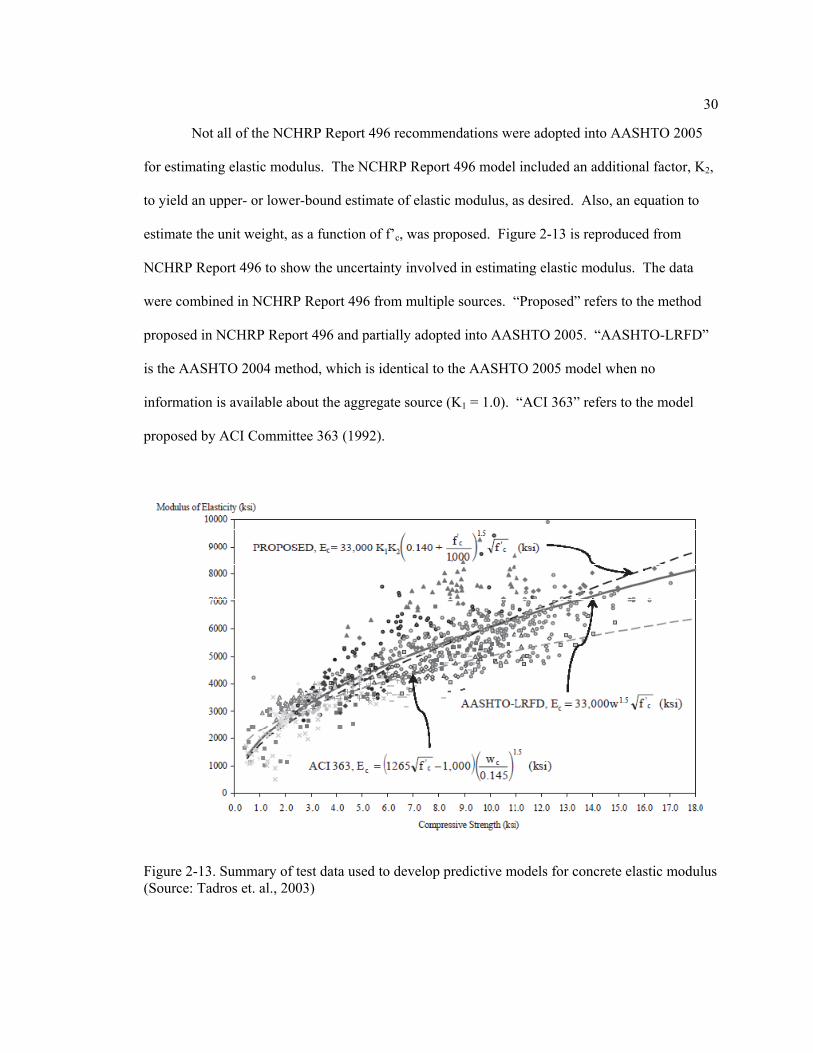
Not all of the NCHRP Report 496 recommendations were adopted into AASHTO 2005
for estimating elastic modulus. The NCHRP Report 496 model included an additional factor, K2,
to yield an upper- or lower-bound estimate of elastic modulus, as desired. Also, an equation to
estimate the unit weight, as a function of f’c, was proposed. Figure 2-13 is reproduced from
NCHRP Report 496 to show the uncertainty involved in estimating elastic modulus. The data
were combined in NCHRP Report 496 from multiple sources. “Proposed” refers to the method
proposed in NCHRP Report 496 and partially adopted into AASHTO 2005. “AASHTO-LRFD”
is the AASHTO 2004 method, which is identical to the AASHTO 2005 model when no
information is available about the aggregate source (K1 = 1.0). “ACI 363” refers to the model
proposed by ACI Committee 363 (1992).
Figure 2-13. Summary of test data used to develop predictive models for concrete elastic modulus (Source: Tadros et. al., 2003)

31
2.4. Relaxation of Prestressing Steel
Relaxation is a loss of stress in the prestressing steel when held at a constant strain. The
strands typically used in practice today are called “low-relaxation” strands. They undergo a strain
tempering stage in production that heats them to about 660oF and then cools them while under
tension (Barker and Puckett, 2007). This process reduces relaxation losses to approximately 25%
of that for stress-relieved strand. The models used by both AASHTO 2004 and AASHTO 2005
rely on the work of Magura (1964).
2.4.1. Estimating Intrinsic Relaxation
In the case of a pretensioned concrete girder, the prestressing strand is not held at
constant strain because the actions of elastic shortening, shrinkage and creep of the concrete
reduce the tension strain in the steel. The intrinsic relaxation of the steel – assuming the strain is
held constant – must be considered in developing a procedure to estimate prestress loss. Magura
(1964) developed the formula reproduced in (2-30), which estimates relaxation as a function of
stress in the strand and the length of time the stress is maintained.
450.55 log
24 124 1
(2-30)
Where:
Intrinsic relaxation loss between t1 and t2 (days)
Stress in prestressing strands at the beginning of the period considered
Yield strength of strands
Age of concrete at the end of the period (days)
32
Age of concrete at the beginning of the period (days)
2.5. Modulus of Elasticity of Prestressing Steel
The elastic response of prestressing is less uncertain than that of concrete. Both
AASHTO 2004 and AASHTO 2005 recommend use of 28500 ksi for the prestressing steel elastic
modulus.
2.6. Summary
Material properties for low-relaxation prestressing steel are well-defined and their
treatment in design specifications has not changed in recent years. Concrete materials properties,
however, are highly variable. Recent changes to the AASHTO LRFD Bridge Design
Specifications have brought about new models for the time-dependent behavior of concrete. The
new models, which followed the recommendations of NCHRP Report 496, are specifically aimed
at defining the behavior of high strength concrete. The material property models are fundamental
to any method used for estimating time-dependent behavior and prestress loss.
Chapter 3
Approximate Time-Dependent Analysis
The methods used by engineers in the design of prestressed concrete bridge girders to
predict time-dependent effects are often based on a set of simplifications that are intended to
approximate reality. Time-dependent analysis is complicated because concrete shrinkage and
creep, along with steel relaxation, lead to partial loss of the initial prestressing force. As the load
history of the girder is considered, there are numerous stress reversals that further complicate the
analysis, especially for concrete creep.
A detailed time-step analysis, discussed in Chapter 4, is often too complex for use in
design. Therefore, simplified methods have been developed to estimate prestress loss. The
estimate of losses is then used in predicting extreme fiber concrete stresses.
This chapter summarizes the AASHTO 2004 and AASHTO 2005 (detailed and
approximate) models, as well as the method of the Canadian Highway Bridge Design Code, S6-
06 (CSA, 2006). These models represent common practice for bridge design in North America.
3.1. AASHTO 2004
The AASHTO 2004 model divides the time-dependent components leading to prestress
losses into three categories: 1) Shrinkage of concrete, 2) Creep of concrete, and 3) Relaxation of
steel. Barker and Puckett (1997) provide a thorough development of these provisions. A
summary is provided in this section.

34
3.1.1. Loss due to Shrinkage
Hooke’s Law requires that the loss of prestress be equal to the product of the elastic
modulus of prestressing steel and the change in strain at the level of the prestressing centroid.
This development assumes perfect bond between the steel and concrete.
Δ (3-1)
Where:
Δ Loss of prestress due to concrete shrinkage
Elastic modulus of prestressing steel
Shrinkage strain of concrete at the level of prestressing steel
The AASHTO 2004 model estimates shrinkage strain by equation (2-6). The correction
factor for specimen size, ks, can be taken approximately equal to 0.7 if assumptions are made for
time (500 days, since most shrinkage has occurred by then) and V/S ratio (3.75, which is common
for bridge girders). The humidity correction factor, kh, is reproduced in (2-8). Taking the
humidity adjustment, kh, approximately equal to 1.7 0.015 , a constant value of 0.7 for ks,
and 28,500,000 psi for Ep in (3-1) yields an expression for prestress loss due to shrinkage, shown
in (3-2). Rounding leads to the equation in the Specifications (AASHTO, 2004).
Δ 17110 151 17000 150 (3-2)
35
3.1.2. Loss due to Creep
As with shrinkage, Hooke’s Law can be used to derive an expression for creep losses.
Since creep is a stress-related phenomenon, concrete stress at the centroid of prestressing must be
known in order to calculate creep strain. Stress changes in concrete are split into two categories
for the AASHTO 2004 method: 1) Stresses introduced at prestress transfer, , and 2) Stresses
introduced at deck placement or later Δ . The total concrete stress at the centroid of
prestressing is the sum of those two terms, recognizing that they will have opposite directions.
Δ (3-3)
Where:
Concrete stress at center of gravity of prestressing at transfer
Δ Change in concrete stress at the centroid of prestressing due to permanent loads applied after transfer
As demonstrated by (2-16), a time-dependent effective modulus for concrete can be
defined as a function of the creep coefficient:
,
, (3-4)
It follows from (3-4) that a time-dependent expression for the modular ratio between
prestressing steel and concrete can be expressed:
,
,, (3-5)
Multiplying together the modular ratio and the concrete stress at the prestressing centroid
estimates the loss of prestress. A different modular ratio will apply to the two terms because the

36
stresses are applied at different times. In this approach, full creep recovery is assumed when the
direction of stress reverses.
Δ , , , , , , Δ (3-6)
Where:
, Creep modular ratio at transfer
, Age of concrete at transfer
, Creep modular ratio for permanent loads
, Age of concrete when permanent loads are applied
The creep coefficient is different in the two modular ratio terms because the stress is
induced at different times. AASHTO 2004 uses (2-23) to calculate the creep coefficient. The
series of assumptions shown in Table 3-1 leads to reproduction of the code provision.
Table 3-1. Assumptions in the AASHTO LRFD (2004) creep loss prediction
T Maturity of concrete, days 365
H Relative humidity, % 70
V/S Ratio – volume:surface area, in 3.75
Ep Modulus of Elasticity, prestressing steel, ksi 28500
ti Concrete age at transfer, days 5
f’ci Concrete strength at transfer, ksi 3.5
Eci Concrete modulus of elasticity at transfer, ksi 3400
td Concrete age when deck is cast, days 30
f’c Concrete strength when deck is cast, ksi 5
Ec Concrete modulus of elasticity when deck is cast, ksi 4000

37
As in the assumptions leading to a shrinkage provision, the specimen size factor (kc) can
take a constant value of 0.7. Substituting the assumptions of Table 3-1 into (2-23) yields (3-7) for
creep coefficient after one year when load is applied at the time of transfer.
365,5 3.5 0.7
1
0.67 9
1.58
70120
5 . 365 .
10 365 . 1.47
(3-7)
Referencing (3-5), (3-7), and Table 3-1, the effective modular ratio at transfer is
approximately 12.3.
, 365,5 365,5
285003400
1.47 12.3 (3-8)
Similar to (3-7) and (3-8), the creep coefficient and effective modular ratio for stresses
applied at an age of 30 days (the assumed time of deck placement) are shown in (3-9) and (3-10),
respectively.
365,30 1.03 (3-9)
, 365,30 365,30
285004000
1.03 7.3 (3-10)
Substituting (3-8) and (3-10) into (3-6) and rounding yields the AASHTO 2004 provision
for creep losses:
Δ 12.3 7.3Δ 12 7Δ (3-11)

38
3.1.3. Loss due to Steel Relaxation
In AASHTO 2004, two components of relaxation are considered – that occurring before
transfer, and that after transfer. The relaxation losses at transfer are calculated as the intrinsic
relaxation of the prestressing steel using a form of (2-30). The estimate of relaxation losses after
transfer considers the interaction of prestress losses to reduce the stress in the strands and reduce
the total relaxation loss. Elastic shortening and friction have a larger effect on relaxation because
they occur early in the life of the girder. Since shrinkage and creep occur over time their effect is
smaller. Relaxation loss after transfer for stress-relieved strands can be estimated by (3-12).
20.0 0.4Δ 0.3Δ 0.2 Δ Δ (3-12)
Where:
Δ Loss of prestress due to relaxation after transfer
Δ Loss of prestress due to elastic shortening
Δ Loss of prestress due to friction
Δ Loss of prestress due to shrinkage
Δ Loss of prestress due to creep
In the case of low-relaxation strands, the prestress loss due to relaxation can be taken as
30% of (3-12).

39
3.2. S6-06 Canadian Highway Bridge Design Code
The S6-06 Canadian Highway Bridge Design Code (CSA, 2006) estimates prestress loss
in a format similar to that of AASHTO 2004. Like AASHTO 2004, S6-06 separates time-
dependent losses into the categories of shrinkage, creep, and relaxation.
3.2.1. Loss due to Shrinkage
The S6-06 estimate of shrinkage losses is identical to that of AASHTO 2004. The
equation is shown in (3-2).
3.2.2. Loss due to Creep
The long-term estimate of creep loss in S6-06 is based largely on the work of Zia et. al.
(1979), which proposed (3-13)
Δ (3-13)
Where:
= 2.0 for pretensioned girder; = 1.6 for post-tensioned girder
Modulus of elasticity of prestressing strands
Modulus of elasticity of concrete at 28 days
Net compressive stress in concrete at center of gravity of tendons immediately after the prestress has been applied to the concrete
Stress in concrete at center of gravity of tendons due to all superimposed permanent dead loads that are applied to the member after it has been prestressed

40
S6-06 revises this formula only to include an adjustment factor for relative humidity,
based on recommendations of the PCI Committee on Prestress Losses (1975). The adjustment
factor, shown in (3-14), can be applied to (3-13).
1.37 0.77 0.01 (3-14)
3.2.3. Loss due to Steel Relaxation
Like AASHTO 2004, S6-06 separates relaxation losses into components before and after
transfer. Prior to transfer, the methods for estimating relaxation are identical to AASHTO 2004,
again based on (2-30). After transfer, S6-06 considers the effect of inelastic strains in the
concrete. Based on the work of Grouni (1973 and 1978), S6-06 uses (3-15) to estimate relaxation
losses after transfer for low-relaxation strands, in megapascals.
0.55 0.34
1.25 30.002 (3-15)
Where:
Loss of prestress due to relaxation after transfer
Stress in the prestressing steel at transfer
Specified tensile strength of prestressing steel
Loss of prestress due to creep
Loss of prestress due to shrinkage

41
3.3. AASHTO 2005
The time-dependent analysis (prestress loss) method of AASHTO 2005 was adopted into
the specification following recommendation in NCHRP Report 496 (Tadros et. al., 2003).
Although the impetus of that research program was to extend applicability of the prestress loss
provisions to high strength concrete, the time-dependent analysis method is independent of any
material property assumptions. The AASHTO 2005 material property model is intended for use
with the time-dependent analysis method for high strength concrete applications, although it
could be equally implemented with any material model.
The AASHTO 2005 prestress loss method is more refined that its predecessor
(AASHTO, 2004) in four ways.
1) Rather than lumping all time-dependent effects into a single time increment, the
AASHTO 2005 method divides time-dependent behavior into two periods – before
deck placement and after deck placement.
2) AASHTO 2005 explicitly represents the effect of internal restraint against creep and
shrinkage of concrete by the bonded prestressing steel. A transformed section
coefficient is used to model the behavior.
3) The creep response of concrete to the gradual stress changes that occur as prestress
forces decrease over time is modeled using the age-adjusted effective modulus of
concrete. This concept is introduced in Section 2.2.
4) Differential shrinkage between the precast girder and cast-in-place deck results in a
theoretical prestressing gain. The AASHTO 2005 method marks the first time this
behavior has been included in the specification.
42
Points 1) and 2) affect the AASHTO 2005 model as a whole, and are discussed before
detailing each of the components considered. Application of the AASHTO 2005 method for
design is presented by Al-Omaishi, et. al. (2009).
3.3.1. Stages for Analysis
The AASHTO 2005 model divides the long-term analysis of a composite girder into two
phases. The model first considers the non-composite stage of behavior, prior to deck placement,
and the composite phase is considered separately. Figure 3-1, from NCHRP Report 496,
summarizes the sequence of steps that contribute to changes in the prestressing force over time.
1. {A-C} Loss due to prestressing bed anchorage seating, relaxation between initial
tensioning and transfer, and temperature change from that of the bare strand to
temperature of the strand embedded in concrete.
2. {C-D} Instantaneous prestress loss at transfer due to prestressing force and self-weight.
3. {D-E} Prestress loss between transfer and deck placement due to shrinkage and creep of
girder concrete and relaxation of prestressing strands.
4. {E-F, G-H} Instantaneous prestress gain due to deck weight on the noncomposite section
and superimposed dead loads on the composite section.
5. {H-K} Long-term prestress losses after deck placement due to shrinkage and creep of
girder concrete, relaxation of prestressing strands, and deck shrinkage.

43
Figure 3-1. Timeline representing the change in prestressing force over time in a typical prestressed member (Source: Tadros, 2003)
Total time-dependent losses are found by summing components, as shown in (3-16). The
elastic gains due to load application are not considered.
∆ ∆ ∆ ∆
∆ ∆ ∆ ∆ (3-16)
Where:
∆ Loss due to shrinkage of girder concrete between transfer and deck placement
∆ Loss due to creep of girder concrete between transfer and deck placement
∆ Loss due to relaxation of prestressing strands between time of transfer and deck placement
∆ Loss due to relaxation of prestressing strands in composite section between time of deck placement and final time

44
∆ Loss due to shrinkage of girder concrete between time of deck placement and final time
∆ Loss due to creep of girder concrete between time of deck placement and final time
∆ Prestress gain due to shrinkage of deck in composite section
Sum of time-dependent prestress losses between transfer and deck placement
Sum of time-dependent prestress losses after deck placement
3.3.2. Transformed Section Coefficient
AASHTO 2005 uses a transformed section coefficient to model the internal restraint that
bonded prestressing imparts on the surrounding concrete against shrinkage and creep. The
coefficient itself is a value less than 1.0 that represents the ratio of actual change in strain,
considering the restraint provided by the prestressing steel, to the change in strain that
would occur with no restraint. It is denoted by Kid for the non-composite stage of
behavior and Kdf after casting of a composite deck. The formulation of the transformed
section coefficient is similar for both shrinkage and creep, before and after deck
placement. For demonstration here, the term will be derived with respect to shrinkage
prior to deck placement.
The derivation refers to Figure 3-2. The shrinkage strain distribution across the
girder section is affected by the presence of bonded prestressing steel. is the “free”
shrinkage strain of concrete that would exist without any internal restraint. denotes the
reduction in shrinkage strain, at the centroid of the prestressing, caused by the steel’s

45
restraint. The transformed section coefficient is the ratio of the net strain to the “free”
strain.
(3-17)
Figure 3-2. Schematic diagram demonstrating the effect of steel restraint on concrete shrinkage
In developing an equation for Kid, it will be assumed that the rate of shrinkage is uniform
over the entire cross section. The concrete will undergo a “free” shrinkage, . Compatability
requires that the same strain exist in the steel. Therefore, shrinkage of the concrete exerts a
compressive force, P, on the steel equal to:
(3-18)
Where:
Effective compression force applied to the prestressing steel by the shrinkage strain of concrete
Total area of prestressing steel

46
Modulus of elasticity of prestressing steel
Unrestrained shrinkage strain of concrete
Considering equilibrium, a tension force must be applied to the cross section by the
prestressing steel. The force can be represented as the sum of two components – the portion
applied to the gross concrete section and the portion applied to the prestressing steel. The
component of that force applied to the gross concrete section can be determined by recognizing
that resulting stresses must satisfy the relationship in (3-19).
(3-19)
Where:
The portion of the restraint force effectively applied to the concrete component of the cross section
Gross area of concrete
Moment of inertia, based on the gross concrete section
Eccentricity of the prestressing steel centroid in the section considered, usually midspan
Portion of the total shrinkage strain restrained by the bonded prestressing steel, at the centroid of the prestressing
Elastic modulus of concrete at the time of prestress transfer
Solving (3-19) for the component of the force on the concrete:
1
(3-20)
Where:

47
1 (3-21)
The second component of the restraint force, applied to the prestressing steel, is shown in
(3-22).
(3-22)
Where:
The portion of the restraint force effectively applied to the prestressing steel component of the cross section
Summing the concrete and steel components and setting them equal to the compression
force exerted by shrinkage on the steel (force equilibrium) yields (3-23).
(3-23)
Shrinkage is not instantaneous, but occurs gradually with time. Therefore, the stresses
due to restrained shrinkage are partially relieved by concrete creep. To represent the fact that the
force, P, builds gradually over time, the age-adjusted effective modulus, , will replace the
concrete elastic modulus, .
1 , (3-24)
Where:
“Relaxation coefficient” (Trost, 1967) which accounts for the reduction in creep that occurs because not all of the stress is applied at the initial time, ti (Collins, 1991). Values typically range between 0.6 and 0.9.

48
, Creep coefficient at time, t, due to stresses induced at time, ti
Substituting the age-adjusted effective modulus into (3-23):
1 , (3-25)
Solving for the strain restrained by the bonded prestressing steel, :
1
1 ,
1 11 ,
(3-26)
Where:
(3-27)
(3-28)
Substituting (3-26) into (3-17) and simplifying leads to the form of the equation
incorporated into the AASHTO 2005 model.
1
1 1 , (3-29)
The AASHTO 2005 model adopts a constant value of 0.7 for the relaxation coefficient, ,
as recommended by Dilger (1982).

49
3.3.3. Analysis Before Deck Placement
Time-dependent analysis of the non-composite phase is separated into three components
leading to prestress loss – shrinkage, creep, and relaxation.
3.3.3.1. Loss Due to Girder Shrinkage
Prestress loss due to shrinkage is determined by Hooke’s Law using the net shrinkage
strain at the prestressing centroid as described in Section 3.3.2 and depicted in Figure 3-2. The
format used by AASHTO 2005 is given in (3-30).
Δ (3-30)
Where:
Concrete shrinkage strain of girder between the time of transfer and deck placement [Eq. 5.4.2.3.3-1]
Transformed section coefficient that accounts for time-dependent interaction between concrete and bonded steel in the section being considered for time period between transfer and deck placement
Modulus of elasticity of prestressing steel (ksi)
3.3.3.2. Loss Due to Girder Creep
Again from Hooke’s Law, the equation for losses due to girder creep is very similar to
that for shrinkage loss.
Δ (3-31)

50
Where:
Unrestrained creep strain of girder concrete
Recalling (2-14), creep strain is determined by the product of the creep coefficient and
the elastic stress in the concrete. The stresses prior to deck placement are caused primarily by the
initial prestress and the self-weight of the girder. Calculating the elastic stress at the centroid of
the prestressing and the creep coefficient for the time of deck placement allows for a prediction of
creep strain, shown in (3-32).
, (3-32)
The creep loss equation of AASHTO 2005 is reproduced by substituting (3-32) into (3-
31).
∆ , (3-33)
Where:
Ep Modulus of elasticity of prestressing steel (ksi)
Eci Modulus of elasticity of concrete at transfer (ksi)
fcgp Sum of concrete stresses at the center of gravity of prestressing tendons due to the prestressing force at transfer and the self-weight of the member at the sections of maximum moment (ksi)
td Age at deck placement (days)
ti Age at transfer (days)
Kid Transformed section coefficient that accounts for time-dependent interaction between concrete and bonded steel in the section being considered for time period between transfer and deck placement

51
ψb(td,ti) Girder creep coefficient at time of deck placement due to loading introduced at transfer
3.3.3.3. Loss Due to Steel Relaxation
Losses due to strand relaxation from transfer to deck placement can be given as:
Δ (3-34)
If the ratio 0.55
0.55 log
24 124 1
(3-35)
If 0.55 relaxation losses are assumed to be zero
The reduction factor, , which accounts for the steady decrease in strand tension due to
creep and shrinkage losses, is given by Tadros (1977):
1
3 Δ Δ (3-36)
Where:
Stress in prestressing strands just after transfer
Specified yield strength of strands
Age at deck placement (days)
Age at transfer (days)
Transformed section coefficient that accounts for time-dependent interaction between concrete and bonded steel in the section being

52
considered for time period between transfer and deck placement
= 45 for low-relaxation steel; = 10 for stress-relieved steel
AASHTO 2005 allows designers to assume a total relaxation loss of 2.4 ksi, as there
tends to be small variability in this term. It is recommended that half of the total loss be assigned
to the time period before deck placement, and half afterwards.
3.3.4. Analysis After Deck Placement
AASHTO 2005 divides the time-dependent change in prestress into four components for
the composite phase after deck placement – girder shrinkage, creep, relaxation, and differential
shrinkage between the deck and the girder.
3.3.4.1. Loss Due to Girder Shrinkage
Prestress loss due to girder shrinkage after deck placement is determined similar to
shrinkage losses for the non-composite girder case. From Hooke’s Law:
∆ (3-37)
Where:
Concrete shrinkage strain of girder between the time of deck placement and final time
Transformed section coefficient that accounts for time-dependent interaction between concrete and bonded steel in the section being considered for time period between deck placement and final time
Modulus of elasticity of prestressing steel (ksi)

53
Kdf is derived in the same manner as Kid (refer to Section 3.3.2), except that it is relative
to the full composite section.
1
1 1 1 0.7 ,
(3-38)
3.3.4.2. Loss Due to Girder Creep
The AASHTO 2005 equation for creep loss after deck placement is presented in (3-39).
∆ , ,
Δ , 0.0 (3-39)
Where:
Modulus of elasticity of prestressing steel
Modulus of elasticity of girder concrete at transfer
Modulus of elasticity of girder concrete
Sum of concrete stresses at the center of gravity of prestressing tendons due to the prestressing force at transfer and the self-weight of the member at the sections of maximum moment
Transformed section coefficient that accounts for time-dependent interaction between concrete and bonded steel in the section being considered for time period between deck placement and final time
Δ Change in concrete stress at centroid of prestressing strands due to long-term losses between transfer and deck placement, combined with deck weight and superimposed loads

54
, Girder creep coefficient at final time due to loading introduced at transfer
, Girder creep coefficient at time of deck placement due to loading introduced at transfer
, Girder creep coefficient at final time due to loading at deck placement
Equation (3-39) separates the creep strain into two components: 1) Creep caused by the
initial prestressing force and the girder self-weight – some of which already occurred prior to
deck placement, and 2) creep in the opposite direction caused by deck self-weight and
superimposed dead loads. The creep coefficient difference term, , , ,
represents the amount of creep that remains to occur during the time from deck casting to final
time, considering the elastic stresses at the centroid of prestressing due to initial conditions, .
The second term represents a creep “gain” (assuming Δ is negative, as typical) due to
the tension induced (decrease in compression) at the centroid of the prestressing strands. The
tension stress increment results from prestress losses during the phase prior to deck placement
and flexural stresses caused by additional permanent loads, including deck self-weight. A
different creep coefficient, , , is used because the stress change occurs at the time of
deck placement, td, rather than initial time, ti. This approach, by superimposing creep strains due
to both tension and compression stress increments, inherently assumes full creep recovery.
3.3.4.3. Loss Due to Steel Relaxation
As indicated in Section 3.3.3.3, AASHTO 2005 permits an assumption of 2.4 ksi for total
losses due to relaxation, with half of that amount (1.2 ksi) attributed to the time period after deck
placement.

55
3.3.4.4. Gain Due to Deck Shrinkage
In typical composite construction, which bonds a precast girder with a cast-in-place deck,
internal stresses develop because of the differing rates of shrinkage between the two components.
Since the girder is precast, and most shrinkage strain occurs during the early ages of the concrete
(Section 2.1), much of the shrinkage strain occurs prior to deck casting. Therefore, only the small
portion of remaining shrinkage strain occurs during the composite phase of behavior. The cast-
in-place deck, however, experiences all of its shrinkage during the composite phase. This
differential in the composite section – the deck shrinks more than the girder – induces an effective
compression force on the composite section at the level of the deck centroid. A tension strain at
the opposite face of the girder (the bottom) follows. The elongation leads to an increase in the
prestress force. AASHTO 2005 estimates the prestress gain by (3-40).
Δ Δ 1 0.7 , (3-40)
Where:
Modulus of elasticity of prestressing steel
Modulus of elasticity of concrete
Δ Change in concrete stress at centroid of prestressing strands due to shrinkage of deck concrete
Transformed section coefficient that accounts for time-dependent interaction between concrete and bonded steel in the section being considered for time period between deck placement and final time
, Girder creep coefficient at final time due to loading at deck placement
The age-adjusted effective modulus is used in (3-40) because the shrinkage differential
builds gradually.

56
AASHTO 2005 provides an equation for Δ that will be derived for clarity. The
derivation will be based on the generic cross section shown in Figure 3-3 where the deck is above
the neutral axis of the composite section and the center of gravity of the prestressing force is
below the neutral axis.
Figure 3-3. Generic composite cross-section to facilitate the derivation of Δfcdf
As the deck shrinks relative to the girder, it applies a compressive force on the composite
section, P’.
(3-41)
Where:
Shrinkage strain of the deck concrete
Effective area of the deck that behaves with the girder in composite action
Modulus of elasticity of deck concrete
Effective compression force on the composite section at the centroid of the deck due to differential shrinkage, as defined by AASHTO 2005

57
Since the force builds over time, the age-adjusted effective modulus, , will be
substituted for . The change in stress due to this effective force at the level of the prestressing
is a combination of axial and flexural effects. Taking strand shortening as positive since that
reflects a prestress loss, the change in stress is:
Δ (3-42)
Where:
Gross area of the composite section
Moment of inertia of the gross concrete section
Eccentricity of the deck, relative to the composite section
Eccentricity of the prestressing centroid, relative to the composite section
Substituting the expression for from (3-41) into (3-42), recalling that , and
combining terms yields the AASHTO 2005 equation for Δ .
Δ1 ,
1 (3-43)
The negative sign in this equation assumes a positive value for ed – true of conventional
cases where the deck is above the neutral axis of the composite section. The Δ term will be
negative in most cases, indicating strand elongation – a gain in prestressing force.

58
3.4. AASHTO 2005 “Approximate Method”
AASHTO 2005 also presents an approximate method for use in preliminary design. It is
a lump sum approach based on the detailed method (Section 3.3), but some simplifications and
assumptions are made to arrive at an abbreviated equation. First, to summarize the detailed
method, total losses are based on (3-44).
ΔΔ
Δ 1
(3-44)
The authors of NCHRP Report 496 arranged the equation such that the first two terms
relate to shrinkage of the girder, the last two terms relate to relaxation of the strands, and all the
terms in between deal with creep. Differential shrinkage is not considered. The following is a
summary of the assumptions made to arrive at the “approximate method”. A full description is
provided by Tadros et. al. (2003).
1) For low-relaxation strands, the total relaxation loss is roughly 2.4 ksi
2) The total shrinkage loss can be estimated as 12 ksi assuming:
a. Ep = 28500 ksi
b. Typical girder V/S ratios yield ks = 1.0
c. Prestressing is usually transferred at a concrete age of one day, so the loading age
factor can be taken as 1.0
d. Assume Kid = Kdf = 0.8
e. Combining coefficients yields 480 10 28500 0.8 10.94
f. The authors of NCHRP 496 used a coefficient of 12 rather than 10.94 to produce
an upper-bound correlation with the test results

59
3) The creep losses are simplified to the expression 10 through a series of
steps
a. The effect of girder stiffening by composite action will be ignored – the girder
will be assumed non-composite its entire life span
b. The small prestress gain due to deck shrinkage will be ignored
c. Assume Kid = Kdf = 0.8, such that total creep losses could be given by
0.8 Δ 0.8
d. Assume modular ratios ni = 7 and n = 6
e. For a loading age of one day, load duration of infinity and V/S ratio 3in-4in, the
creep coefficient can be expressed as 1.9
f. The creep coefficient for deck loads and superimposed loads is assumed to be
40% of the creep coefficient for initial loads
g. The level of prestress in the girder is related to the stress at the level of the
prestressing by assuming that the prestress force provided yields zero net stress in
the bottom fibers at service load. It is further assumed the stress is a result of
three equal components from girder self-weight, deck weight, and live load
The approximate method is ultimately given by (3-45).
Δ 10.0 12.0 2.5 (3-45)
Where:
1.7 0.01 (3-46)

60
51
(3-47)
3.5. Discussion
Concerns have been expressed (Walton and Bradberry, 2004) about the complex nature
of the AASHTO 2005 method, relative to the other methods. Designers have grown accustomed
to the AASHTO 2004 method that separates long-term prestress losses into three components and
concrete stresses are then determined from fundamental mechanics once an effective prestressing
force is known. The increased complexity of the calculations in AASHTO 2005 suggests greater
precision. Prestress losses are highly variable and dependent on many factors. Therefore, it may
be unreasonable to expect a great deal of precision in a model.
3.5.1. Stages for Analysis
The division of time-dependent behavior into two phases complicates the AASHTO 2005
model, relative to the others. It effectively doubles the computational effort, and it requires the
designer to estimate the value of more variables. In particular, AASHTO 2005 requires the
designer to assign an age for the variable, td, that represents the age of the girder when the deck is
cast. The sequence of construction – especially the time of deck placement relative to production
of the girder – is highly variable and difficult for the engineer to anticipate at the time of design.
The time-dependent analysis in Chapters 4 and 5 provide justification for the removal of the td
variable and for combining the two phases for design calculations.
61
3.5.2. Transformed Section Coefficient
The transformed section coefficient, Kid, for use with shrinkage and creep prior to deck
placement was derived in Section 3.3.2 and the format shown in the Specifications (AASHTO,
2005) is reproduced in (3-48).
1
1 12
1 0.7 ,
(3-48)
Two terms in (3-48) are inconsistent with its fundamental derivation. First, the Kid
transformed section coefficient is intended to represent the behavior of the girder concrete, when
partially restrained against shrinkage and creep by bonded prestressed steel, prior to the time of
deck placement. Therefore, the age-adjusted effective modulus should be determined using the
creep coefficient at the time of deck placement, , , rather than that for final time,
, . Secondly, the internal redistribution of stresses that occurs when the prestressed steel
resists shrinkage and creep strains is partially dependent on the modular ratio between steel and
concrete. Over time stresses will distribute with respect to the modular ratio of steel and “final
time” concrete. Therefore, the modular ratio should be replaced by .
The formulation for Kdf, the transformed section coefficient for composite section, has
similar inconsistencies. The AASHTO 2005 format of the equation is given in (3-38). This
coefficient is intended for use in the time period after deck placement. The inelastic strains occur
during the composite phase of behavior. Therefore, the age-adjusted effective modulus used in
development of Kdf should introduce the creep coefficient at final time for stresses induced at the
time of deck placement, , , rather than , . Also, as presented in the previous
paragraph, the modular ratio should be with respect to the final time concrete elastic modulus.
Additionally, derivation of Kdf, similar to Kid, assumes that shrinkage strain is constant over the

62
cross section. This assumption is not valid during the composite phase because differential
shrinkage between the girder and deck is typical. Separate consideration of deck shrinkage
partially compensates for this inconsistency.
Furthermore, with respect to both Kid and Kdf, the age-adjusted effective modulus used in
the derivation represents behavior attributed to creep. Therefore, use of these coefficients to
represent internal stress redistribution due to shrinkage is not entirely accurate because it partially
combines actions due to creep with the shrinkage component. For the case of shrinkage, the
internal stress redistribution that occurs because of the restraint of the bonded prestressing steel
would be exactly the same regardless of whether shrinkage occurs instantaneously or over time,
in the absence of creep. It would be better to use a transformed section coefficient very similar to
Kid and Kdf that does not include the age-adjusted effective modulus if trying to explicitly separate
shrinkage and creep components.
3.5.3. Differential Shrinkage
The AASHTO 2005 model introduces an estimate of prestress “gain” due to shrinkage
differential between the girder and the deck. It was noted in Section 3.3.4.4 that the effective
force in the deck – acting in compression on the composite section – will produce elongation in
the prestressing strands and an elastic gain in force. The language of the Specification
(AASHTO, 2005) can create confusion, however, because differential shrinkage also induces
tension stress on the bottom of the girder. If the prestress gain due to differential shrinkage is
superimposed with prestress losses due to the other components, and the resulting effective
prestressing force is used to calculate extreme fiber concrete stresses, an error results. The elastic
gain in prestressing due to differential shrinkage does not act to further pre-compress the bottom
face of the girder. This effect is similar to the elastic gain observed (refer to Figure 3-1) when

63
load is applied to the girder. These gains, although they are real, are not considered when
calculating extreme fiber stresses. A tension increment on the bottom face of the girder
accompanies the elongation of the prestressing strands in responding to applied load.
Furthermore, approximating the effective force that differential shrinkage applies to the
composite section should be done considering the difference in shrinkage strains between the
girder and the deck after deck placement. The formulation in (3-41) suggests that is a function
of total deck strain. It should, instead, be based on the difference, , where
represents the shrinkage strain in the girder after deck placement.
Finally, the transformed section coefficient, Kdf, should not be applied in considering
differential shrinkage as shown in (3-40). The transformed section coefficient applies when creep
or shrinkage of the concrete is partially restrained by bonded prestressing steel. In the case of
differential shrinkage, however, an effective force is applied to the entire cross section. The
bonded prestressing responds elastically, but does not cause an internal redistribution of stresses.
3.5.4. Transformed Section Properties
As documented by Ahlborn et. al. (2000), there are various recommendations for the use
of transformed section properties in calculating concrete stresses. Generally speaking, although
the use of transformed section properties is more exact, gross or net section properties can be
used in practice with little error (Lin and Burns, 1981). Stresses in the concrete section can then
be calculated through a combined stress calculation of the general form (compression indicated
negative):
(3-49)

64
Where:
Prestressing force at the stage of interest
Eccentricity of the centroid of prestressing with respect to the girder centroid
Location of concrete layer for which stress is being calculated, relative to the girder centroid
Gross moment of inertia
Gross cross-sectional area
Applied moment due to external loading
Transformed section properties can be used for a more accurate calculation of concrete
stresses (Hennessey and Tadros, 2002), although no formal recommendation was adopted into the
Specifications (AASHTO, 2005). In calculating transformed section properties, the steel area is
multiplied by a factor 1 in which n is the modular ratio, . The (-1) term reflects the fact
that steel is replacing an equivalent area of concrete. The transformed section can be represented
schematically in Figure 3-4. Concrete is shown in light gray, while steel that has been
transformed to an equivalent area of concrete is shown darker.
Figure 3-4. Transformed cross section, shown schematically

65
Since the steel generally falls closer to the face of the beam controlled by a tension stress
limit, using transformed section analysis reduces the extreme fiber tensile stress (because the
theoretical neutral axis location shifts closer to the tension face) and reduces the prestressing
demand (Hennessey and Tadros, 2002). By this reasoning, it is generally conservative to use
gross section properties for stress analysis of pretensioned concrete members.
Hennessey and Tadros (2002) state that: “Prestress loss estimates by AASHTO (2004)
formulas were based on the assumption that gross section properties are used in the concrete
stress analysis. Unless these formulas are modified, transformed section analysis may be
incorrect and misleading. If the proper loss components are accounted for, the difference in
results between the approximate gross section analysis and the more accurate transformed
section analysis is not expected to be large.”
In other words, prestress methods of the past had been “calibrated” to consider the fact
that engineers would be using gross section properties in design because of the lack of computing
power needed to make transformed section analysis efficient.
When using a transformed section analysis, elastic effects such as elastic shortening due
to transfer or elastic gains when external loads are applied will be automatically accounted for in
the calculation of extreme fiber stress – but must be explicitly calculated if the effective prestress
force is needed. Example problems illustrating this concept are provided by Hennessey and
Tadros (2002) and Walton and Bradberry (2004).

Chapter 4
Analysis Methods
Two analysis methods are developed in this chapter for use later in this study. First, a
time-step method is developed to facilitate a detailed time-dependent analysis of pretensioned
concrete girders. The detailed analysis will serve as a baseline for comparing other methods and
for developing a simplified approach. Second, the Monte Carlo simulation techniques used for
the uncertainty analysis in this thesis are developed and documented.
4.1. Detailed Time-Step Method
In determining the accuracy and variability of prestress loss prediction methods, an
“exact” solution is needed as a baseline. Many experimental studies have been done in this area,
but reliable test data are difficult to obtain because measuring prestress losses is challenging, as
evidenced by the highly variable test data summarized in the literature (Tadros et. al., 2003).
Even if the prestress losses can be measured correctly, the various components cannot be
separated with any certainty due to the combination of elastic and inelastic strains. Therefore, a
detailed time-step analysis was developed to discern the sensitivity of key variables and to
validate a simplified procedure.
The girder is discretized into horizontal layers representing the concrete component. One
layer, at the level of the prestressing centroid, is dedicated to representing the presence of bonded
steel in the cross section. At each step in the time history of the girder a strain distribution that
satisfies compatability and equilibrium is calculated considering inelastic effects (i.e. creep,
shrinkage, and relaxation) and the elastic response to applied loads. With the strain distribution at

67
each step known, the change in strain at the level of prestressing can be found, leading to an
estimate of prestress loss.
4.1.1. Assumptions
A time step algorithm is developed so that a theoretically precise baseline solution, for a
given set of assumptions, can be obtained. The time step routine allows tracking not only of
prestress losses, but also of bottom fiber concrete stresses which are often the designer’s end goal
in flexural design.
The algorithm is based on the following assumptions:
Creep effects are additive for both increasing and decreasing stress increments
(creep superposition)
A creep recovery factor that scales the creep function in the case of decreasing
compression stress increments can be included to allow for less than full creep
recovery
Stresses are constant for an entire time step
Strain compatability requires perfect bond between the concrete and prestressing
steel (the strain in the steel matches the strain in the concrete at the same level)
Plane sections remain plane
Shrinkage is uniform through the cross section
Material properties, as detailed in Chapter 2, are based on published models

68
4.1.2. Development of the Method
Figure 4-1 graphically shows the relationship between increments of stress, creep, and
total strain. All effects contributing to strain up to the time of interest are summed to find the
total strain. Schematically, all of the stress changes are shown positive, but the stress increments
may also reverse. In the case of stress reversal, full creep superposition is assumed unless a creep
recovery factor is applied. The total stress-related strain – elastic effects and creep – is
determined by superposition of the strain due to each stress increment in the time history of the
concrete.
(4-1)
Where:
Total stress-related strain at time, t
Total stress-related strain at time, t, due to the ith stress increment
The creep compliance function expresses the total elastic and creep strain as a function of
elastic modulus and creep coefficient for a unit stress, as shown in (4-2).
,
1 1, (4-2)
Where:
, τ Creep compliance function – total stress-related strain at time, t, due to a stress increment at time,
, Creep coefficient at time, t, for a stress increment at time, τ
Modulus of elasticity of concrete at time,

69
Figure 4-1. Schematic of the creep compliance relationship
The total strain at time, t, due to a series of stress increments can be written in terms of
the stress of each increment and the corresponding creep compliance function as shown in (4-3),
or in simplified form as in (4-4).
Δ τ C t, τ Δσ τ C t, τ Δσ τ C t, τΔσ τ C t, τ (4-3)
Δ , (4-4)
Where:
, Creep compliance function – total stress-related strain at time, t, due to a stress increment at time,

70
Δ Increment of stress induced at time,
Not all time-dependent strain in concrete is stress-induced. Shrinkage strain must also be
considered. Temperature strain will be disregarded for this study because temperature changes
will have a similar effect on both concrete and steel, therefore not impacting prestress losses.
(4-5)
Where:
Total strain at time, t
Elastic strain at time, t
Creep strain at time, t
Shrinkage strain at time, t
Creep and shrinkage effects can be lumped together and termed “inelastic.”
(4-6)
Where:
Total inelastic strain at time, t
Substituting (4-6) into (4-5) yields (4-7).
(4-7)
Rearranging (4-7) to solve for the elastic strain yields (4-8).
(4-8)
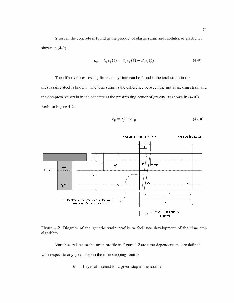
71
Stress in the concrete is found as the product of elastic strain and modulus of elasticity,
shown in (4-9).
(4-9)
The effective prestressing force at any time can be found if the total strain in the
prestressing steel is known. The total strain is the difference between the initial jacking strain and
the compressive strain in the concrete at the prestressing center of gravity, as shown in (4-10).
Refer to Figure 4-2.
(4-10)
Figure 4-2. Diagram of the generic strain profile to facilitate development of the time step algorithm
Variables related to the strain profile in Figure 4-2 are time-dependent and are defined
with respect to any given step in the time-stepping routine.
Layer of interest for a given step in the routine

72
Area of layer k
Total area of prestressing steel
Total deck thickness
Total girder height
Vertical location of layer k, relative to the top of the deck
Vertical location of the prestressing centroid, relative to the top of the deck
Reference strain at time used to define the strain profile
Reference curvature at time used to define the strain profile
Reference strain at the time of deck placement, including the elastic response of the girder to the deck weight
Reference curvature at the time of deck placement, including the elastic response of the girder to the deck weight
Total strain in layer k
Change in strain in the prestressing steel due to time-dependent effects
Equivalent strain used to model the loss of stress due to steel relaxation
Initial jacking strain in the prestressing steel
Effective jacking strain in the prestressing steel, considering losses due to relaxation which are modeled as a reduction to the initial jacking strain
Total effective strain in the prestressing steel
The effective jacking strain in the prestressing steel is denoted , where an effective
strain representing the relaxation of steel is subtracted from the initial jacking strain.
The sign convention for the method is established by Figure 4-2. Tension strain in the
prestressing steel is positive, while compression/shortening strain in the concrete is positive. As
shortening strain in the concrete increases over time (i.e. creep or shrinkage), the strain in the
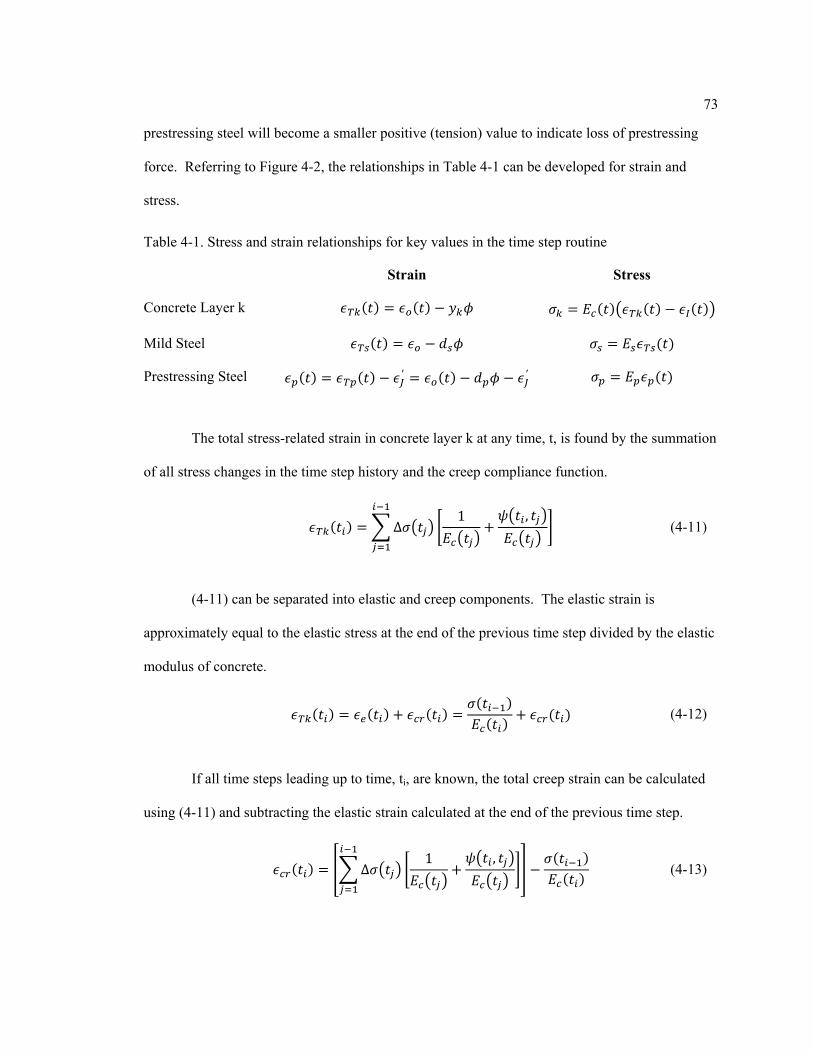
73
prestressing steel will become a smaller positive (tension) value to indicate loss of prestressing
force. Referring to Figure 4-2, the relationships in Table 4-1 can be developed for strain and
stress.
Table 4-1. Stress and strain relationships for key values in the time step routine
Strain Stress
Concrete Layer k
Mild Steel
Prestressing Steel ′ ′
The total stress-related strain in concrete layer k at any time, t, is found by the summation
of all stress changes in the time step history and the creep compliance function.
Δ
1 , (4-11)
(4-11) can be separated into elastic and creep components. The elastic strain is
approximately equal to the elastic stress at the end of the previous time step divided by the elastic
modulus of concrete.
(4-12)
If all time steps leading up to time, ti, are known, the total creep strain can be calculated
using (4-11) and subtracting the elastic strain calculated at the end of the previous time step.
Δ
1 , (4-13)

74
Recall the shrinkage strain is assumed constant over the cross section. Shrinkage strain
will be calculated with respect to the chosen material property model. Creep and shrinkage strain
can be combined as total inelastic strain.
Recognizing that the cross-section must be in equilibrium, and that the applied axial force
is zero, the total axial force, N, in the section must sum to zero at any time after transfer.
0 (4-14)
Practically, the equilibrium expression in (4-14) will be satisfied by considering the stress
in each concrete layer k and the effective stress in prestressing steel. The equilibrium expression
is expanded in (4-15) using the relationships summarized in Table 4-1.
0 (4-15)
The reference strain and curvature are substituted into (4-15) to reduce the total number
of unknowns in the equation. Refer to Table 4-1.
0
(4-16)
Grouping terms in (4-16) with respect to reference strain and reference curvature
produces (4-17).

75
(4-17)
(4-17) takes the general form of (4-18).
(4-18)
Where:
(4-19)
(4-20)
(4-21)
(4-22)
NI and NP are effective axial forces representing the internal stresses due to creep and
initial strand tension, respectively.
For layers representing deck concrete (assuming the deck to be composite) additional
considerations are needed. The calculations must reflect the fact that a “zero strain” case for the
deck corresponds to an existing strain and curvature in the girder at the time of deck placement

76
(after deck weight has been applied to the girder, assuming unshored construction). Referring to
Figure 4-2, and are the reference strain and curvature, respectively, for the girder at the
time of deck placement. This line serves as the datum for calculations in deck layers. Therefore
the equilibrium equation must be adjusted slightly, as shown in (4-23).
(4-23)
Where:
Strain in layer k at the time of deck placement (after deck loading has been introduced, but before deck stiffness is considered)
The form of (4-18) changes with the addition of another term.
(4-24)
Where:
(4-25)
Similar steps must be taken to ensure that flexural equilibrium is satisfied. The internal
moment in the cross section must equal the external moment due to applied loads.
(4-26)
Expanding (4-26) to include forces due to concrete and prestressing steel components
yields (4-27).

77
(4-27)
Where:
Total moment from external loads; taken negative for moments that induce compression on top of the beam
Substituting the reference strain and curvature (see Table 4-1) into (4-27) and combining
terms produces (4-28).
(4-28)
(4-28) takes the general form of (4-29).
(4-29)
Where:
(4-30)
(4-31)

78
(4-32)
(4-33)
MI and MP are effective moments due to internal stresses associated with concrete creep
and initial tension in the prestressing strands, respectively.
Similar to the equations for axial force equilibrium, special considerations are needed for
deck layers. (4-34) is derived similar to (4-24) and can be used for deck layers when analyzing
flexural equilibrium.
(4-34)
Where:
(4-35)
A strain profile that satisfies equilibrium is found by simultaneous solution of (4-18) and
(4-29) before deck placement or (4-24) and (4-34) after deck placement. The solution yields the
reference strain and curvature for the time step under consideration, from which the strain at any
location in the section can be determined. Once the strain is known, the stress at any layer is
found by Hooke’s Law, shown in (4-36).
(4-36)

79
4.1.3. Algorithm
The following is an outline of the algorithm used to solve for the strain profile and
stresses in each layer in any given time step. Computer code to execute the algorithm repeatedly
has been developed in VBA and run through Microsoft Excel for use in this study.
1. Calculate the stress at each level k
a. In the typical time step (not step 1) this is the stress found at the end of the
previous step. At step 1, all layers begin with zero stress.
2. Calculate the creep strain at each level k
a. The total creep strain is based on the stress increment and creep coefficient
corresponding to that increment for each step leading up to the current age. This
requires an assumption about creep superposition. Either full superposition can
be applied, or a creep recovery factor can be defined.
3. Add shrinkage strain to creep strain to find the total inelastic strain for each level k
4. Calculate the constants for the simultaneous equations (4-18) and (4-29) or (4-24) and (4-
34).
5. Solve simultaneous equations to yield reference strain and curvature for the current time
step
6. Solve for the total strain at each level k, based on the reference strain and curvature
7. Find total strain in the prestressing steel from Equation 4-10
8. Find the elastic stress at each level k by taking the difference between total strain and
inelastic strain
9. Calculate the stress increment compared with the previous step to be used in future creep
calculations
10. Repeat the algorithm for the next time step

80
A detailed example demonstrating the implementation of the time step routine to a simple
problem is provided in Appendix B.
4.2. Monte Carlo Simulation
Monte Carlo simulation involves repeatedly cycling different values for each uncertain
input parameter through a numerical model. The values for the uncertain input parameters are
determined from its probability distribution. For models with many input parameters, such as
prestress loss methods, one value from each is sampled simultaneously in each repetition of the
simulation. (Cullen and Frey, 1999).
Monte Carlo simulation can be summarized concisely by the following steps:
Identify the base input variables for the numerical model
Develop a distribution to represent the uncertainty inherent in each input variable
Establish the numerical model that connects the input variables to yield the desired output
For each cycle in the simulation, generate a random number (between zero and one) for
each independent variable
Using the cumulative distribution function (CDF) for each input variable, a value can be
assigned to the variable for the current simulation cycle based on the random number
generated
The model output, based on the randomly selected input variable values, is stored and
compiled with results from all other simulation cycles
The collection of the model outputs from all cycles can be used to fit a distribution
representing the inherent uncertainty in the model
The process is shown schematically in Figure 4-3.

81
1.0 1.0
Pro
babi
lity
Dis
trib
utio
n F
unct
ion
(PD
F)
Cum
ulat
ive
Dis
trib
utio
n F
unct
ion
(CD
F)
Input 1 Input 2
Numerical Model for Estimating Prestress Loss
Prestress Loss Estimate: PSi
Run 1: PS1
Run 2: PS2
Run 3: PS3
...Run i: Psi
…Run N: PSN
Estimated Prestress LossPro
babi
lity
Den
sity
Fun
ctio
n
Parameter 1 Parameter 2
Develop a distribution to represent
uncertainty for each input parameter
Express the distribution for each
parameter in terms of cumulative probability
Use a random number generator to select a value from the CDF for each parameter in each simulation cycle
Use the randomly selected input values in the
numerical model for estimating prestress losses
Save the prestress loss estimate for all cycles in
the simulation
Use the data from all the simulation cycles to
develop a distribution representing uncertainty in prestress loss estimates
Figure 4-3. Schematic of the Monte Carlo simulation technique used for the uncertainty study of prestress loss methods.

82
For the purposes of this study, a Monte Carlo simulation routine was developed in
Microsoft Excel and VBA (Visual Basic for Applications – the programming language used for
Excel macros). Using this technique, most of the calculations are done in the spreadsheet. A
macro is needed only to drive the iterations for subsequent cycles. For each cycle, the macro
generates a random number, using the Microsoft Excel random number generator, for each
variable. Based on that random number, and the cumulative frequency distribution representing
the uncertainty of the variable, a random value for the input variable is determined. Once a value
has been determined for each variable and checked to be within the limits specified (minimum
and maximum values are set by practical criteria), the spreadsheet formulas representing the
numerical model for the prestress loss method calculate the output. In this case, the prestress loss
and bottom fiber stress are the most important output values. Finally, the macro stores all the
input and output information for each cycle in a separate table for data analysis at a later time.
4.3. Summary
This chapter summarizes the development of the time step method used for detailed
analysis of the girder’s time-dependent behavior. This method will be used in subsequent
chapters as a baseline for model comparison, and as the foundation for justifying a simplified
method. The Monte Carlo simulation technique is used in the uncertainty analysis detailed in
Chapter 7.

Chapter 5
Detailed Time-Dependent Analysis
An approximate approach to time-dependent analysis, three of which are summarized in
Chapter 3, is usually preferable for use in design due to the complexity of the problem. In
validating the approximate methods, and in developing a new method, results from a detailed
time-step method are valuable. The time-step method developed in Chapter 4 will be
implemented in this chapter.
5.1. Stages of Behavior
This section summarizes the construction sequence of the typical pretensioned girder and
indicates the effects this sequence has on the time-dependent behavior of the girder. The major
stages of loading are shown in Figure 5-1 and summarized below.
A. Prestressing strands are tensioned between fixed restraints and anchored
B. Concrete is cast around the tensioned strands. Once set, the concrete is bonded to the
prestressed strands.
C. The prestressed strands are cut. The initial force in the prestressing strands is now
transferred to the concrete through bond stresses, introducing a compression force on
the section. The concrete will have an elastic response to this compression load,
causing the beam to shorten. When the beam shortens, some of the initial strain in
the prestressing tendons is lost. With this decreasing strain, the internal force in the
tendons also decreases. In the typical case where the net prestressing effect is
eccentric in the girder cross section an upward deflection (camber) will result. In this

84
condition, the beam is supporting its own selfweight because the ends of the beam are
sitting on the casting bed but the midspan has deflected upwards.
D. In most cases the girder will be stored for weeks or months before being installed at a
bridge site. During this time the beam is resisting a large force from the prestressing
and has only its own selfweight as gravity load. The concrete is undergoing volume
change due to two phenomena – creep and shrinkage. Shrinkage is considered to be
uniform through the cross section, causing the entire beam to shorten. The volume
change due to creep is stress-dependent. Therefore the bottom of the beam
(assuming eccentric prestressing and the beam in positive camber) will tend to
shorten more than the top, causing an increase in camber. The combination of the
creep and shrinkage reduces the strain in the prestressing strands and leads to further
decrease in strand force.
E. The beam is installed in its final location where additional (superimposed) dead load
is applied, typically in the form of a deck slab and other bridge elements. This load
causes a downward deflection and increases the strain at the level of the prestressing,
thus increasing the force in the prestressing tendons. This effect is an elastic “gain”
in prestressing. It should be noted, however, that the superimposed load contributes
tension stress to the bottom face of the girder. Creep and shrinkage of concrete
continue to be important factors for the in-service condition. If the girder was stored
for several months before being installed, there may be very little shrinkage strain
remaining to occur during the service condition. The creep effect, however, is now
reversed. The region of the cross section under the highest compressive stress has
now changed. During stage D most of the creep deformation occurred near the face
of the girder with the highest prestressing effect – generally the bottom. Now the net
compressive stress is more uniform through the cross section as the stresses due to

85
superimposed dead load and due to prestressing eccentricity approximately negate
each other. The girder will continue to shorten, resulting in a decrease in prestressing
force. Also, in many cases the deck will be cast composite with the girder (meaning
shear transfer is provided between the two). An effective force is created by the
differential volume changes between the deck and girder. Since the deck is often
cast-in-place, the fresh deck concrete is bonding to the aged concrete of the girder.
The deck concrete will have more potential for shrinkage strain during their bonded
lifetime because much of the girder’s shrinkage strain has already occurred. This
differential shrinkage effectively applies a compressive force to the composite
section at the level of the deck centroid.
F. When live loads (service loads) are applied, the prestressing strands experience an
elastic gain while the bottom face of the girder receives additional tensile stress. This
stress should be calculated based on the composite section properties if the deck is
behaving compositely with the girder.
The stages of behavior can be further described by the changes to the strain and stress
distributions in the cross section due to each effect. The effects on prestressing force and
concrete stress have been separated into eleven components for presentation here. The following
figures (5-2 through 5-10) summarize changes in strain and stress due to each component. It
should be recognized that the bonded prestressing steel in the cross-section provides restraint to
creep and shrinkage in the concrete. This restraint causes a redistribution of stress. Any mild
reinforcement will have the same restraining effect, although it is not considered for the purposes
of this study. This omission is reasonable because the amount of prestressing steel is usually
much greater than the amount of mild reinforcement in the primary flexural direction.
Additionally, the mild reinforcement will typically be distributed across the section with

86
Figure 5-1. Stage of loading for a pretensioned concrete girder - manufacturing through service.
little net eccentricity. In the case of a partial prestressed design, special considerations may be
warranted. The sequence of figures presented here is a conceptual look at the system to aid in
understanding the problem. In the case of steel relaxation, stress is lost in the strand without a
change in strain. In practice, the stress loss due to relaxation is very small. Therefore the internal

87
stress redistribution due to relaxation is also very small. While relaxation losses will be
considered, the corresponding redistribution of stresses internally will be ignored as negligibly
small.
An attempt has been made to indicate the relative magnitudes of the different components
graphically, but in some cases scale has been sacrificed for clarity of the graphic.
1. Initial Prestressing Force
Figure 5-2. Strain and stress in the girder cross section due to initial prestressing force
2. Girder Self-Weight
Figure 5-3. Strain and stress in the girder cross section due to girder self-weight

88
3. Girder shrinkage prior to deck placement
Figure 5-4. Strain and stress in the girder cross section due to shrinkage prior to deck placement
4. Girder creep prior to deck placement
Figure 5-5. Strain and stress in the girder cross section due to creep prior to deck placement
5. Relaxation of steel prior to deck placement
Relaxation involves a decrease of stress in the steel without corresponding change in
strain. Compared to other components, relaxation losses are relatively small. The changes in
stress and strain over the cross section due to relaxation are minor.

89
6. Deck self-weight
Figure 5-6. Strain and stress in the girder cross section due to deck self-weight
7. Shrinkage after deck placement
Effects due to shrinkage after deck placement are complicated by the fact that the girder
and deck are shrinking at different rates. Much of the girder shrinkage has already taken place by
this time, but all of the deck shrinkage will be redistributed in the composite section. It is
common for the differential shrinkage to lead to a theoretical gain in prestressing force, but a
corresponding tension stress at the girder bottom fiber.
Figure 5-7. Strain and stress in the girder cross section due to shrinkage after deck placement

90
8. Super-imposed dead load on the composite section
Figure 5-8. Strain and stress in the girder cross section due to superimposed dead load on the composite section
9. Creep after deck placement
After the deck has been cast, the girder will continue to creep. In some cases, it may
“recover” some of the creep from before deck placement because of the stress reversal. Creep
effects in the deck concrete are very small because it is under relatively small stress. The creep
gain shown in the graphic could also be a creep loss, depending on the exact nature of the system
and the age of the girder concrete when the deck is cast. Creep of the deck concrete acts to
“soften” the effect of differential shrinkage between the deck and the girder.
Figure 5-9. Strain and stress in the girder cross section due to creep after deck placement

91
10. Relaxation of prestressing strands after deck placement
As indicated in point 5, relaxation losses are small compared to the other components.
11. Live Load
Figure 5-10. Strain and stress in the girder cross section due to live load
5.2. Example Bridge Details
The prestress loss methods are compared for a given set of numerical input, and the time-
step method results are shown with respect to a particular set of input parameters. Two bridges
have been identified for use in this study because they represent typical pretensioned bridge
girder construction and full design calculations are readily available. One is Design Example 9.4
in the PCI Bridge Design Manual (PCI, 1997) and the other is from the Comprehensive Design
Example for Prestressed Concrete Girder Superstructure Bridge with Commentary (FHWA,
2003). They will be referred to as “PCI BDM Example 9.4” and “FHWA Example,”
respectively.
The PCI BDM Example 9.4 bridge will be the primary example used in this study. Since
loss of prestress is determined by an analysis of the critical cross section, it is not necessary to
study a broad range of bridges within a single structure type classification. The FHWA Example

92
is used as a comparison to validate the simplified method developed in this thesis because it has a
smaller initial prestress and is therefore less affected by creep losses. The basic design
parameters of both bridges are summarized in the following sections.
5.2.1. PCI BDM Example 9.4
The bridge consists of six 120-ft simple span 72-in. deep AASHTO-PCI bulb-tee girders
spaced at 9 feet. An 8-in. thick composite deck is cast-in-place on the girders. Relevant design
data is presented in Table 5-1.
Table 5-1. Parameters for the PCI BDM Example 9.4 Bridge (Source: PCI, 1997)
Average ambient relative humidity, H 70%
Girder concrete strength at release, f’ci 5.8 ksi
Girder concrete strength at service, f’c 6.5 ksi
Deck concrete strength at service, f’cd 4 ksi
Total Area of Prestressing, Aps 7.344 in2
Prestressing Eccentricity at Midspan, em 29.68 in
Prestressing Stress at Transfer, fpbt 202.5 ksi
Girder gross area, Ag 767 in2
Girder gross moment of inertia, Ig 545894 in4
Girder centroid, relative to girder bottom, yb 36.6 in
Effective width of deck, beff 108 in
Width of haunch 42 in
Height of haunch 0.5 in

93
The bridge section is shown in Figure 5-11, followed by the girder section in Figure 5-12.
Figure 5-11. Bridge section for PCI BDM Example 9.4 (Source: PCI, 1997)
Figure 5-12. Girder section for PCI BDM Example 9.4 (PCI, 1997)
The applied loads are summarized in terms of midspan moment in Table 5-2.

94
Table 5-2. Summary of moments at midspan (k-in) for PCI BDM Example 9.4 (Source: PCI, 1997)
Dead Load Live Load plus Dynamic Load
Allowance
Non-composite Composite Composite
Girder, Mg Slab, Md MSIDL MLL
17258 19915 6480 32082
The modulus of elasticity for concrete, calculated by the AASHTO 2004 method, is
summarized for each component in Table 5-3.
Table 5-3. Concrete elastic modulus for PCI BDM Example 9.4 (Source: PCI, 1997)
Girder (Transfer) 4383 ksi
Girder (Service) 4640 ksi
Deck 3640 ksi
The composite section properties, using an effective deck width of 108 inches, are
summarized in Table 5-4.
Table 5-4. Composite section properties for PCI BDM Example 9.4 (Source: PCI, 1997)
Composite Area 1419 in2
Composite Moment of Inertia 1100306 in4
Location of neutral axis, relative to girder bottom
54.77 in
Eccentricity of Prestress 47.85 in
5.2.2. FHWA Example
The FHWA (Wassef et. al., 2003) example bridge consists of a reinforced concrete deck
supported on simple span prestressed girders made continuous for live load. There are two spans
of 110-feet each. Relevant design data is provided in Table 5-5.

95
Table 5-5. Parameters for the FHWA Example Bridge (Source: FHWA, 2003)
Average ambient relative humidity, H 70%
Girder concrete strength at release, f’ci 4.8 ksi
Girder concrete strength at service, f’c 6 ksi
Deck concrete strength at service, f’cd 4 ksi
Total Area of Prestressing, Aps 6.732 in2
Prestressing Eccentricity at Midspan, em 31.38 in
Prestressing Stress at Transfer, fpbt 202.5 ksi
Girder gross area, Ag 1085 in2
Girder gross moment of inertia, Ig 733320 in4
Girder centroid, relative to girder bottom, yb 36.38 in
Effective width of deck, beff 111 in
Width of haunch 42 in
Height of haunch 1 in
The bridge section is shown in Figure 5-13, followed by the girder section in Figure 5-14.
Figure 5-13. Bridge section for FHWA Example (Source: FHWA, 2003)

96
Figure 5-14. Girder section for FHWA Example (Source: FHWA, 2003)
The applied loads are summarized in terms of midspan moment in Table 5-6.
Table 5-6. Summary of moment at midspan (k-in) for the FHWA Example (Source: FHWA, 2003)
Dead Load Live Load plus Dynamic Load
Allowance
Non-composite Composite Composite
Girder, Mg Slab, Md MSIDL MLL
20142 21984 4608 24120
The modulus of elasticity for concrete, calculated by the AASHTO 2004 method, is
summarized for each component in Table 5-7.

97
Table 5-7. Concrete elastic modulus for the FHWA Example (Source: FHWA, 2003)
Girder (Transfer) 4200 ksi
Girder (Service) 4696 ksi
Deck 3834 ksi
The composite section properties, using an effective deck width of 111 inches, are
summarized in Table 5-8.
Table 5-8. Composite section properties for the FHWA Example (Source: FHWA, 2003)
Composite Area 1419 in2
Composite Moment of Inertia 1100306 in4
Location of neutral axis, relative to girder bottom
54.77 in
Eccentricity of Prestress 47.85 in
5.3. Components of Time-Dependent Behavior
The PCI BDM Example 9.4 bridge is used in this section to demonstrate the time step
analysis method. The AASHTO 2005 material property model is used for each analysis. Figure
5-15 plots the effective prestress in the girder over time assuming the deck is cast at an age of 90
days. Note that Figure 5-15 matches the general behavior anticipated, shown in Figure 3-1.
The effective prestress loss shown in Figure 5-15 by the time-step method is compared
with the results yielded by the AASHTO 2005 method for the same design. Two cases are
plotted: 1) the case where elastic gains are included in the estimate of prestress, and 2) the case,
typically used in design, where elastic gains are ignored. The comparison is shown in Figure 5-
16.

98
Figure 5-15. Effective prestress over time for PCI BDM Example 9.4 assuming deck casting at 90 days
The prestress losses for the PCI BDM Example 9.4 (when the deck is cast at 90 days) are
plotted in Figure 5-17. The time step model allows explicit separation of the components by the
following sequence of analyses:
1. The first analysis considers only the initial prestressing force. All time-
dependent effects and applied loads, including girder self-weight, are ignored.
This analysis determines the effect due to initial prestressing.
2. The second analysis considers only the initial prestressing force and applied
loads, ignoring time-dependent effects. The difference between the second and
first analyses yield the effect due to external loads.
0
50
100
150
200
250
0 50 100 150 200 250
Eff
ec
tiv
e P
res
tre
ss
(k
si)
Time (days)
Jacking stress
Loss at transfer due to elastic shortening
Loss prior to deck placement due to creep, shrinkage, and relaxation
Elastic gain due to application of deck weight
Elastic gain due to application of superimposed dead load
Loss after deck placement due to creep, shrinkage, and relaxation coupled with an elastic gain due to differential shrinkage between the girder and deck

99
Figure 5-16. Comparison between the time-step results and the AASHTO 2005 method for effective prestress in the PCI BDM Example 9.4 bridge, assuming the deck is cast at 90 days
3. The third analysis includes initial prestressing, applied loads, and girder
shrinkage. Once the deck concrete is included in the analysis, after the time of
deck casting, the shrinkage of the deck is artificially taken equal to the girder
shrinkage. In this manner, differential shrinkage can be isolated as a separate
component. Difference between the third and second analyses yields the effect
due to shrinkage.
4. The fourth analysis includes initial prestressing, applied loads, girder shrinkage,
and deck shrinkage. The difference between the fourth and third analyses yields
the effect due to differential shrinkage.
0
50
100
150
200
250
0 50 100 150 200 250
Eff
ec
tiv
e P
res
tre
ss
(k
si)
Time (days)
Time Step Method
AASHTO 2005 Method (including elastic gains)
AASHTO 2005 Method (ignoring elastic gains)

100
5. The fifth analysis includes all contributors to time-dependent behavior: initial
prestressing, external loads, girder shrinkage, deck shrinkage, relaxation, and
creep. Relaxation and creep are both stress-dependent, so they cannot be
explicitly separated. Since relaxation effects are small by comparison, they will
be isolated first to minimize error. Analysis 5 represents the “total” effect.
6. The sixth analysis includes all effects from the fifth analysis, except creep. The
calculated relaxation losses over time in the fifth analysis are artificially copied
into the sixth analysis. The difference between Analysis 6 and Analysis 4 yields
the effect due to relaxation. The difference between Analysis 5 and Analysis 6
yields the effect due to creep.
Figure 5-17 presents the results of the six analysis steps indicated for the PCI BDM
Example 9.4 bridge.
For flexural design, the bottom fiber concrete stress is often the controlling factor. The
time step procedure also allows tracking of the bottom fiber stress. The components have been
split in the same manner as indicated above, and the results are shown in Figure 5-18.
One should note, in Figure 5-18, the small impact on bottom fiber stress of creep,
shrinkage, relaxation, and differential shrinkage relative to the applied loads and initial
prestressing. Additionally, in comparing Figures 5-17 and 5-18, note that differential shrinkage
causes a prestressing gain, but a tension increment at the bottom fiber. This distinction is
important in applying the provisions of AASHTO 2005 (see Section 3.3.4.4), and in considering a
simplified procedure.

101
Figure 5-17. Components of prestress loss for the PCI BDM Example 9.4 bridge assuming the deck is cast at 90 days
‐20
‐10
0
10
20
30
40
50
0 50 100 150 200 250
Pre
str
es
s L
os
s (
ks
i) [
Po
sit
ive
= P
/S L
os
s;
Ne
ga
tiv
e =
P/S
Ga
in]
Time (days)
Initial Prestressing
External Loads
Girder Shrinkage
Deck-Girder Dif ferential Shrinkage
Steel Relaxation
Creep
Total
Color Key:

102
Figure 5-18. Components of bottom fiber stress for the PCI BDM Example 9.4 bridge assuming the deck is cast at 90 days
5.4. Time of Deck Placement
The time-step method is useful in determining the impact the construction schedule has
on the total loss of prestress, with respect to the girder age when the deck is cast. As discussed in
Section 3.5.1, the AASHTO 2005 method separates the time-dependent into two stages – before
and after deck placement. The analysis summarized in Figures 5-17 and 5-18 is repeated for
cases when the deck is cast early in the construction sequence (girder age of 30 days) and late in
the sequence (girder age of 365 days). The results are compared with the analysis for deck
casting at 90 days in Figure 5-19 for prestress losses and Figure 5-20 for bottom fiber stress.
‐5
‐4
‐3
‐2
‐1
0
1
2
3
0 50 100 150 200 250
Bo
tto
m F
ibe
r S
tre
ss
at
Mid
sp
an
(k
si)
[P
os
itiv
e I
nd
ica
tes
Te
ns
ion
]
Time (days)
Initial Prestressing
External Loads
Girder Shrinkage
Deck-Girder Dif ferential Shrinkage
Steel Relaxation
Creep
Total
Color Key:

103
Figure 5-19. Comparison of prestress loss components for different times of deck placement in the PCI BDM Example 9.4 bridge
Figures 5-19 and 5-20 indicate that the time of deck placement has minimal impact on the
time-dependent behavior of the girder, assuming full creep recovery. Splitting the time-
dependent analysis into phases before and after deck placement, as done by the AASHTO 2005
method, complicates the analysis and introduces a variable that engineers are not likely to know
at the time of design. These analysis results suggest that the division between the two phases is
not necessary.
In examining the bottom fiber stress results in Figure 5-20, it’s apparent that the small
difference in bottom fiber stress due to changing the time of deck placement is entirely attributed
to the differential shrinkage component. Therefore, if the two phases are combined in a
‐20
‐10
0
10
20
30
40
50
0 100 200 300 400 500 600 700 800 900 1000
Pre
str
es
s L
os
s (
ks
i) [
Po
sit
ive
= P
/S L
os
s;
Ne
ga
tiv
e =
P/S
Ga
in]
Time (days)
Initial Prestressing
External Loads
Girder Shrinkage
Deck-Girder Dif ferential Shrinkage
Steel Relaxation
Creep
Total
Color Key:
Deck cast at 30 days
Deck cast at 90 days
Deck cast at 365 days
Linetype Key:

104
Figure 5-20. Comparison of prestress loss components for different times of deck placement in the PCI BDM Example 9.4 bridge
simplified analysis, a conservative assumption for the time of deck placement should be made.
Conservative, in this case, would be a late age for deck casting because greater shrinkage
differential exists.
To further justify combining the two phases in the analysis and eliminating the time-of-
deck-placement variable, a range of practical values are studied in the AASHTO 2005 method.
Figure 5-21 shows the total effective prestress estimated by the AASHTO 2005 method when
considering a range of deck placement times for the PCI BDM Example 9.4 bridge. These results
further justify the removal of the time-of-deck-placement variable because less than a 1.0 ksi
‐5
‐4
‐3
‐2
‐1
0
1
2
3
0 100 200 300 400 500 600 700 800 900 1000
Bo
tto
m F
ibe
r S
tre
ss
at
Mid
sp
an
(k
si)
[P
os
itiv
e I
nd
ica
tes
Te
ns
ion
]
Time (days)
Initial Prestressing
External Loads
Girder Shrinkage
Deck-Girder Dif ferential Shrinkage
Steel Relaxation
Creep
Total
Color Key:
Deck cast at 30 days
Deck cast at 90 days
Deck cast at 365 days
Linetype Key:

105
difference in effective prestress is observed for a range of deck placement times from 30 days to
365 days.
Figure 5-21. Total effective prestress estimated by AASHTO 2005 over a range of deck placement times for the PCI BDM Example 9.4 bridge
5.5. Irreversible Creep
In development of the simplified methods for time-dependent analysis presented in
Chapter 3, full creep recovery is assumed. The calculations are built around the premise that a
compressive stress increment will cause elastic strain instantaneously, followed by additional
creep strain over time. It is also assumed that for a later tension stress increment (i.e. unloading
of the compressive stress) the elastic strain is fully recovered and the creep strain is recovered
154.0 154.0 154.0 153.9 153.8 153.6 153.5 153.4
0
50
100
150
200
250
0 50 100 150 200 250 300 350 400
Effective prestress after all losses estim
ated
by AASH
TO 2005 (ksi)
Time of Deck Placement (Days)
Initial Prestress

106
fully according to the creep coefficient once updated for the concrete age at the time of the stress
change. Figure 5-22 offers a schematic of elastic and creep strains in concrete.
Figure 5-22. Creep of concrete when loaded and unloaded (Source: Mehta and Monteiro, 2006)
Although it is beyond the scope of the current research program to quantify the effects of
creep recovery, it is helpful to determine the impact of irreversible creep on prestress loss and
extreme fiber stresses in order to provide guidance for future research. An approach will be used
here similar to the two-function method proposed by Yue and Taerwe (1993) to predict concrete
creep under decreasing stress. As a simplification, the function to represent creep recovery will
be the same as the function to predict creep but multiplied by a scalar. Since creep under
decreasing stress is less than creep under increasing compressive stress, the scalar will be a value
less than one. Note, again, that the AASTHO 2005, AASHTO 2004, and S6-06 methods assume
this scalar to be equal to one.

107
Since the purpose here is only to gauge the significance of creep recovery on the long-
term estimate of extreme fiber stresses, a scale factor of 0.75 will be used. This value is chosen
somewhat arbitrarily, although it is a realistic and practical value. Again the analysis will apply
to the PCI BDM Example 9.4 bridge.
Time-dependent plots are provided to compare creep recovery factors of 75% and 100%
for both prestress loss (Figure 5-23) and bottom fiber stress (Figure 5-24) assuming 90 days for
the time of deck placement. The analysis was done with the time step method using the
AASHTO 2005 material models.
Figure 5-23. Impact of creep recovery factor on effective prestress for the PCI BDM Example 9.4 bridge
168.8
165.3
0
50
100
150
200
0 50 100 150 200 250
Effective Prestress (ksi)
Time (days)
Creep Recovery = 100%
Creep Recovery = 75%
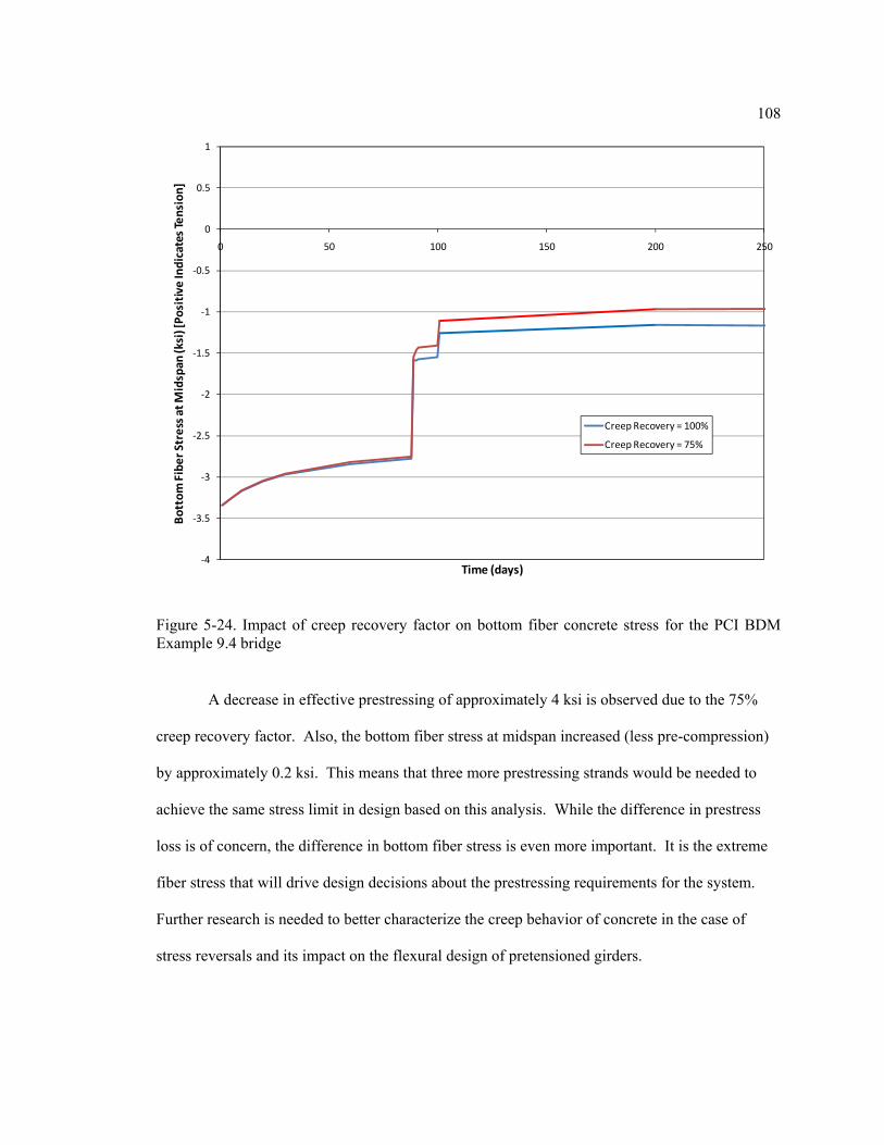
108
Figure 5-24. Impact of creep recovery factor on bottom fiber concrete stress for the PCI BDM Example 9.4 bridge
A decrease in effective prestressing of approximately 4 ksi is observed due to the 75%
creep recovery factor. Also, the bottom fiber stress at midspan increased (less pre-compression)
by approximately 0.2 ksi. This means that three more prestressing strands would be needed to
achieve the same stress limit in design based on this analysis. While the difference in prestress
loss is of concern, the difference in bottom fiber stress is even more important. It is the extreme
fiber stress that will drive design decisions about the prestressing requirements for the system.
Further research is needed to better characterize the creep behavior of concrete in the case of
stress reversals and its impact on the flexural design of pretensioned girders.
‐4
‐3.5
‐3
‐2.5
‐2
‐1.5
‐1
‐0.5
0
0.5
1
0 50 100 150 200 250
Bottom Fiber Stress at Midspan
(ksi) [Positive Indicates Tension]
Time (days)
Creep Recovery = 100%
Creep Recovery = 75%

109
5.6. Summary
The time step method, developed in Chapter 4, is used to analyze the time-dependent
behavior of pretensioned girders, with the PCI BDM Example 9.4 bridge used as a case study.
The time step results, coupled with a sensitivity study of AASHTO 2005, suggest that separating
the time-dependent behavior into phases before and after deck placement is not necessary. Also
the assumption of full creep recovery impacts the estimate of prestress loss and extreme fiber
concrete stress. The time step method results are needed to validate the Direct Method, which is
detailed in Chapters 6 and 7.

Chapter 6
The “Direct Method” for Time-Dependent Analysis
In an attempt to simplify the AASHTO 2005 method, a simplified approach – coined the
“Direct Method” to use separate nomenclature from previous AASHTO specifications – is
derived in the following sections. The scope of applicability for the Direct Method is the same as
the AASHTO 2005 methods, currently in Articles 5.9.5.3 and 5.9.5.4 of the AASHTO LRFD
Bridge Design Specifications (AASHTO, 2005). In order to satisfy a need for comfort and
familiarity with designers, the format of AASHTO 2004 is followed as closely as possible. With
this goal in mind, time-dependent losses are treated in three separate components: creep of
concrete, shrinkage of concrete, and relaxation of prestressing steel. Those components will not
be separated into time steps before and after deck placement, as justified by the analysis and
discussion in Section 5.4.. The differential shrinkage component, first considered by AASHTO
2005, is also included, however, the treatment of differential shrinkage is different in the Direct
Method. The AASHTO method expresses the effect of differential shrinkage in terms of a
prestress gain. This approach creates the possibility of significant calculation errors in design
because the prestress gain cannot be superimposed with the prestress losses and treated in the
same manner. Therefore, the Direct Method will account for differential shrinkage by an
effective force at the deck centroid so that its application will be more intuitive than the current
format and less prone to confusion. The format of the Direct Method, relative to the AASHTO
2004 and AASHTO 2005 methods, is shown in Figure 6-1.

111
Figure 6-1. The format of the Direct Method relative to the AASHTO 2004 and AASHTO 2005 methods
The prestress loss equations can be further simplified if a particular model for creep and
shrinkage is adopted inherently. Although the creep and shrinkage models developed in NCHRP
Report 496, and subsequently adopted as part of AASHTO 2005, may not be fully vetted, those
models will be used in the Direct Method for the following reasons:
1) The models have already been adopted by AASHTO and are currently in the
specifications
2) Although less conservative (predicting smaller creep and shrinkage strains than previous
methods) in some instances, the results from this model have been developed (Tadros,
2003) considering a comparison with other creep and shrinkage predictive methods.
3) There is not a more suitable method available that considers the behavior of high-strength
concrete.

112
4) The choice of a comprehensive creep and shrinkage model is not critical because creep
and shrinkage are small components affecting the bottom fiber stress at final time.
6.1. Elastic Shortening and Steel Relaxation
No changes are proposed to the AASHTO 2005 method regarding elastic shortening
losses and steel relaxation losses. A constant value of 2.5 ksi, as recommended by NCHRP
Report 496, should be used for relaxation of low-relaxation strands.
6.2. Concrete Shrinkage
The effects of concrete shrinkage will be split into two categories:
1) Shrinkage of girder concrete
2) Differential shrinkage between the deck and the girder
Differential shrinkage will be considered as a separate component, with shrinkage of the
girder concrete treated in this section.
Considering the shrinkage of the girder alone, and recognizing that the change in
prestress is the product of steel elastic modulus and the change in strain at the level of the
prestressing centroid (Hooke’s Law), yields the general equation for shrinkage losses in (6-1).
Δ (6-1)
Where:
Elastic modulus of prestressing steel
Unrestrained shrinkage strain of girder concrete from initial to final time

113
The ratio of actual change in strain, considering the restraint provided by the prestressing steel against shrinkage, to the change in strain that would occur with no restraint.
This is comparable to the base equation for shrinkage loss used in AASHTO 2005,
reproduced in (4-30) except that Kid-SH has replaced Kid. Kid-SH is specified so that only the
restraint effects specifically related to shrinkage are represented. The intent of the factor is the
same, but a few adjustments have been made:
1. The “softening” effect represented by the age-adjusted effective modulus is a result of
creep behavior. (refer to Section 2.2 for background on the age-adjusted effective
modulus) If shrinkage and creep components are strictly separated, the results of
shrinkage will be the same regardless of whether the shrinkage happens suddenly or over
a long period of time. Therefore, an age-adjusted effective modulus is not applied to the
case of shrinkage, and the creep term is removed from the Kid equation.
2. The service-level concrete elastic modulus will be used rather than the elastic modulus at
the time of transfer. Over time, stresses will be redistributed according to the final
relative stiffness between concrete and steel, not the initial ratio.
Kid-SH can then be given by (6-2).
1
1 1
(6-2)
For typical pretensioned girders, Kid-SH is approximately 0.9.
Expanding the AASHTO 2005 model equation to estimate the shrinkage of
concrete results in (6-3).

114
1.45 0.13 2.00
0.0145
1 61 40.48 10
(6-3)
Where:
Ratio of volume to surface area for the girder
Ambient relative humidity
′ Compressive strength of girder concrete at transfer
Age of the concrete (in this case the girder concrete)
By adopting this model for shrinkage, the prestress loss provisions become less
flexible because they cannot be adapted for use with other models. The AASHTO 2005
method maintains the flexibility to use other models, sacrificing opportunities for
algebraic simplification.
The following assumptions and simplifications are made:
girder size factor, 1.45 0.13 1.0 for common girder V/S ratios near 3.5
time-development factor, ′ 1.0 when t is very large, as it is for losses
at final time
′ 0.8 ′ as recommended by Tadros, et. al. (2003)
0.9
Incorporarting these assumptions in (6-3) and substituting into (6-1) results in a
simplified equation to predict prestress loss due to girder shrinkage, shown in (6-4).
Δ
1401.3
3.8 10 (6-4)

115
6.3. Differential Shrinkage
Differential shrinkage between the deck and the girder, in the case of composite
construction, should be considered. Furthermore, any provision related to differential
shrinkage adopted into the specifications should be clear so that a non-conservative
conceptual error does not follow. Such a danger exists with the AASHTO 2005 format.
Examine Figure 6-2 for a clarification of these points. When differential shrinkage
occurs – the deck has a potential shrinkage strain greater than that in the girder concrete –
an effective force, Pdeck, builds up in the composite section. This effective force,
depending on the cross-section dimensions, could cause an increase in strain at the level
of prestressing and a theoretical GAIN in prestressing force. It also, in such a case,
would cause an increase in tension stress at the extreme bottom fiber (presuming positive
flexure). If this gain is superimposed with the prestress loss components in calculating
extreme fiber stresses, suggesting that it contributes to pre-compression of the concrete, a
significant error follows.
Figure 6-2. The effective action on the composite section due to differential shrinkage
Therefore, a non-conservative result is possible if differential shrinkage is
considered just in terms of prestressing gain, as recommended by AASTHO 2005. Such

116
language can be applied incorrectly if the designer does not have a thorough
understanding of the impact differential shrinkage has on the entire composite section.
It may lead to a better conceptual understanding if, instead of considering
differential shrinkage by a loss or gain of prestressing, it is considered as an effective
force, Pdeck, applied at the centroid of the deck. The effective force, Pdeck, applied to the
composite section can be calculated as the product of differential shrinkage, the elastic
modulus of the deck, and the area of the deck that behaves compositely with the girder.
The age-adjusted effective modulus of concrete should be used in this case because the
strain differential builds over time and will be partially relieved by concrete creep. The
effective force, Pdeck, can be calculated by (6-5).
1 , (6-5)
Where:
Differential shrinkage between the deck and the girder
Elastic modulus of deck concrete
Effective area of the deck
“Relaxation coefficient” (Trost, 1967) that accounts for the reduction in creep that occurs because not all of the stress is applied at the initial time, ti (Collins, 1991). Values typically range between 0.6 and 0.9. AASHTO (2005) applies a constant value of 0.7 (Tadros, 2003)
, Creep coefficient for deck concrete at final time due to stresses induced at the time of deck placement
In (6-5), the age-adjusted effective modulus (often denoted ) is represented by the
term shown in (6-6).

117
1 , (6-6)
The effects of differential shrinkage can be determined by (6-5) using any suitable
creep and shrinkage model. As an alternative to calculating the creep coefficient and
differential shrinkage strain in (6-5), an approximate procedure is derived in the
following sections based on the AASHTO 2005 model. The following sections detail
development of approximate terms for the differential shrinkage term, the creep
coefficient for deck concrete, and the effective force, Pdeck.
6.3.1. Approximate Calculation of Differential Shrinkage Strain
The differential shrinkage term is the difference between total deck shrinkage and
girder shrinkage after deck placement.
(6-7)
Where:
Shrinkage strain of girder concrete after the time of deck placement
Shrinkage strain of deck concrete
Using the AASHTO 2005 model for concrete shrinkage, the shrinkage of the girder after
the time of deck placement can be found by (6-8).

118
1.45 0.13 2
0.0145
10.48 10 1
61 4
(6-8)
Where:
Shrinkage strain of girder concrete over entire life
Shrinkage strain of girder prior to deck placement
The following simplifications can be made:
Girder size factor, 1.45 0.13 1.0 for common V/S ratios near 3.5
′ 0.8 ′ as recommended by Tadros et. al. (2003)
The age at deck placement, td, will be assumed 150 days. An earlier age
assumption would be less conservative because it would mean more girder
shrinkage takes place after deck casting, reducing the differential between
deck and girder shrinkage. A later age assumption would have little impact.
For the assumption td = 150 days, the product of the concrete strength factor
and the time-development factors can be approximated as follows:
.
. ′ 1. ′ ′
Considering these assumptions in (6-8), girder shrinkage after deck placement can
be estimated in (6-9).

119
6.72 10140
(6-9)
Total deck shrinkage will be estimated considering the following assumptions:
Deck size factor, 1.45 0.13 0.87 representative of a typical V/S
ratio of 4.5 for decks
′ 0.8 ′ as recommended by Tadros et. al. (2003)
The time development factor for final time, ′ 1.0
Applying these assumptions in the AASHTO 2005 model for shrinkage,
reproduced in (6-3), the total deck shrinkage is approximately given by (6-10).
1401.3
3.65 10 (6-10)
Where:
Shrinkage strain of deck concrete after the time of deck placement
′ Compressive strength of the deck concrete
Combining similar terms, simplifying algebraically, and rounding yields (6-11) to
approximate the differential shrinkage between girder and deck.
6.7 10 140
51
1
(6-11)

120
6.3.2. Approximate Calculation of the Deck Creep Coefficient
A simplified creep coefficient for the deck concrete is derived based on the
AASHTO 2005 model for creep, reproduced in (6-12).
, 1.9 1.45 0.13 1.56
0.0085
1 61 4.
(6-12)
The following assumptions and simplifications can be made:
For typical deck geometry, 4.5
′ 0.8 ′ as recommended by Tadros et. al. (2003)
Time-development factor at final time, ′ 1.0
The effective force due to differential shrinkage starts to build up as soon as
the deck concrete begins gaining strength and shrinking. Therefore, the age of
concrete when loading is applied, 1.0 days
Applying these simplifications in (6-12) allows approximating the deck creep
coefficient by (6-13).
, 8.3 10
1951.3
(6-13)
6.3.3. Approximating the Effective Differential Shrinkage Force
Substituting the approximate terms given in (6-11) and (6-13) into the basic formulation
of (6-5) approximates Pdeck, as shown in (6-14).

121
1.2 10
140 51
1
17 1951.3
(6-14)
The inputs required to calculate Pdeck using (6-14) will be known at the time of design.
The effect of differential shrinkage can be quantified by applying the calculated effective force to
the composite (deck concrete, girder concrete, and bonded prestressing steel) cross-section as
indicated by Figure 6-1. Use of this approach improves the transparency of the provision because
it becomes clear that, even though a theoretical prestress gain results, there will be an increase in
bottom fiber tension. The tension stress increment due to Pdeck can be determined by methods of
fundamental mechanics.
6.4. Creep of Concrete
Loss of prestress due to creep can be determined by Hooke’s Law. The change in
prestress is the product of the prestressing steel elastic modulus and the creep strain in the
girder at the level of the prestressing centroid. The strain is adjusted by the transformed
section coefficient to represent the force redistribution caused by the restraint of bonded
steel against creep.
Δ (6-15)
Where:
Elastic modulus of prestressing steel
Creep strain in the girder at the level of the prestressing steel centroid
The ratio of actual change in strain, considering the restraint

122
provided by the prestressing steel against creep, to the change in strain that would occur with no restraint, approximately 0.85. The formulation is identical to that shown in (4-48), except that Ec is substituted for Eci.
Creep strain is expressed as a function of elastic strain and a creep coefficient.
Δ, (6-16)
Where:
Δ Change of stress in the concrete (at the level of the prestressing centroid, in this case)
Elastic modulus of girder concrete
, Creep coefficient at time of interest, t, due to the stress change Δ applied at time, ti
Substituting (6-16) into (6-15) and rearranging produces (6-17).
Δ Δ , (6-17)
There are three key stress changes at the level of prestressing to consider:
1) fcgp – the stress at the centroid of the prestressing just after transfer
2) Δfcdp – the stress change at the centroid of the prestressing due to application
of deck weight and other permanent loads
3) Δfcps – the stress change at the centroid of the prestressing due to shrinkage
and relaxation losses, and differential shrinkage between the deck and girder

123
If the stress changes due to permanent loads and prestress losses are considered to
occur at the time of deck placement, total creep losses can be found by (6-18).
Δ ,
Δ Δ ,
(6-18)
The general equation for the creep coefficient is given in (6-12). The creep
coefficient for stresses induced at transfer can be simplified by the following
assumptions:
′ 0.8 ′ as recommended by Tadros et. al. (2003)
Girder size factor, 1.45 0.13 1.0 representing typical girder V/S ratios
around 3.5
Time-development factor, ′ 1.0 for losses at final time
1 to represent a typical construction cycle where transfer occurs at a concrete
age of 1-day
Applying these assumptions yields (6-19) to approximate the creep coefficient for
stresses introduced at transfer.
, 0.1
1951.3
(6-19)
Where:
, Creep coefficient at final time due to stresses applied at transfer
124
The creep coefficient for stress changes at the time of deck placement can be
simplified with the same assumptions, except that the loading age term, ti, will be taken
as 150 days. This is a relatively conservative value because earlier loading ages would
suggest more creep “recovery” when stresses are reversed. A later loading age has little
effect on the equation. The approximate equation for the creep coefficient is
conveniently half of the creep coefficient for loads applied at transfer.
, 0.05
1951.3
(6-20)
Where:
, Creep coefficient at final time due to stresses applied at the time of deck placement
Applying an approximate value of 0.85 to the Kid-CR term and simplifying yields
(6-21) for total losses due to concrete creep.
Δ 0.04
1951.3
2 Δ Δ (6-21)
6.5. Implementation of the Direct Method
The format of the Direct Method is similar to that of the AASHTO 2004 method. Use of
the proposed Direct Method requires the following sequence of steps:
Calculate the loss of prestress due to elastic shortening. The method for doing so
has not changed as a result of the NCHRP Report 496 recommendations, nor are
changes being proposed as part of the Direct Method
Calculate the loss of prestress due to shrinkage using (6-4)

125
Calculate the loss of prestress due to steel relaxation. No changes are suggested
to the recommendations of NCHRP Report 496. For low-relaxation strands, a
constant value of 2.5 ksi may be assumed for total losses due to relaxation.
Calculate the effective force, Pdeck, due to differential shrinkage using (6-5) or (6-
14)
Calculate the loss of prestress due to creep using (6-21). Stress at the level of
prestressing due to each of the following three components must be calculated:
o Initial prestressing, just after transfer (fcgp)
o Deck weight and other permanent loads (Δfcdp)
o Shrinkage and relaxation losses, and differential shrinkage between the
deck and girder (Δfcps)
Having calculated each of the terms indicated above, the designer can calculate
stress in the extreme concrete fiber by methods of fundamental mechanics as
follows:
o The stress increment due to initial prestressing and girder self-weight can
be determined using the gross girder cross sectional properties and an
effective prestressing force that is the difference between the initial
prestressing force and that lost from elastic shortening. In the typical
case where initial prestressing will cause camber, the self-weight
moment of the girder should be considered.
o The stress increment due to time-dependent loss of prestress can be
found by considering a reduction in prestress force equal to the sum of
shrinkage, creep, and relaxation losses. The extreme fiber stress change
due to these losses can be calculated based on the gross section

126
properties of the girder. Generally speaking, most of the losses will
occur before the girder becomes composite with the deck.
o The stress increment due to deck self-weight (assuming unshored
construction) should be calculated based on the gross section properties
of the girder.
o The stress increment due to super-imposed dead load will typically be
calculated based on the composite girder properties – this assumes that
the deck and girder are behaving compositely when the super-imposed
dead load is applied.
o The stress increment due to differential shrinkage can be calculated by
applying and effective force, Pdeck, at the centroid of the deck (see Figure
4). In determining stresses, the composite section properties should be
used.
o The stress increment due to live load should be calculated based on
composite section properties.
6.6. Numerical Example
In order to demonstrate use of the equations developed for the Direct Method, a
numerical example is presented. The example problem will demonstrate calculation of extreme
fiber concrete stresses at midspan for the PCI BDM Example 9.4 bridge. Details of the bridge are
provided in Section 5.2.1.

127
6.6.1. Differential Shrinkage
The stresses induced by differential shrinkage between the girder and deck are calculated
by determining an effective compressive force applied to the composite section at the centroid of
the deck, Pdeck.
1.2 10
1405
11
171951.3
(6-22)
1.2 10140 70
51 4
16.5
17195 70
1.3 4
831 3640
529.7
(6-23)
6.6.2. Loss of Prestress
Prestress losses are computed for each of four components: elastic shortening, shrinkage,
relaxation, and creep.
6.6.2.1. Loss Due to Elastic Shortening
The calculation of prestress loss due to elastic shortening is unchanged from previous
code provisions. AASHTO-LRFD Equation C5.9.5.2.3a-1 (AASHTO, 2005) is applied as
follows:
Δ (6-24)

128
Δ7.344 202.5 545894 29.68 767 29.68 17258 767
7.344 545894 29.68 767767 545894 4383
2850019.41
(6-25)
6.6.2.2. Loss Due to Shrinkage
Δ
1401.3
3.8 10 (6-26)
Δ 28500
140 701.3 6.5
3.8 10 9.72 (6-27)
6.6.2.3. Loss Due to Relaxation
Δ 2.5 (6-28)
6.6.2.4. Loss Due to Creep
Δ 0.04
1951.3
2 Δ Δ (6-29)
Where:
(6-30)
The effective prestress at transfer, , will be taken as:
Δ 202.5 19.41 183.09 (6-31)

129
7.344 183.09767
7.344 183.09 29.68545894
17258 29.68545894
2.98
(6-32)
Stress change due to application of deck weight and superimposed dead load:
Δ (6-33)
Δ19915 29.68
5458946480 47.85
11003061.36
(6-34)
The stress change due to shrinkage and relaxation losses, and differential shrinkage:
Δ Δ Δ
1 (6-35)
Δ 7.344 9.72 2.51
76729.68
545894530
1419530 21.48 47.85
11003060.38
(6-36)
Substituting into (6-29) and solving yields:
Δ 0.04285004640
195 701.3 6.5
2 2.98
1.36 0.38 16.6 (6-37)
130
6.6.3. Calculation of Bottom Fiber Stress at Midspan: (Tension shown Positive)
The estimates of prestress loss are used to calculate the extreme fiber concrete stress at
midspan.
6.6.3.1. Stress at Transfer
At the time of transfer, both the initial prestressing (minus elastic shortening losses) and
self-weight moment are contributing to bottom fiber stress.
Δ (6-38)
Δ7.344 183.09
7677.344 183.09 29.68 36.6
54589417258 36.6
5458943.27
(6-39)
6.6.3.2. Long-Term Losses
Since the majority of the prestress loss occurs prior to deck placement, the stress is
calculated based on the girder’s gross section properties.
Δ Δ Δ Δ
1 (6-40)
Δ 7.344 9.72 2.5 16.6
1767
29.68 36.6545894
0.70 (6-41)

131
6.6.3.3. Deck Placement
Δ19915 36.6
5458941.34 (6-42)
6.6.3.4. Super-Imposed Dead Load
Δ
6480 54.771100306
0.32 (6-43)
6.6.3.5. Differential Shrinkage
Δ
5301419
530 21.48 54.771100306
0.19
(6-44)
6.6.3.6. Live Load
Δ
32082 54.771100306
1.60 (6-45)
6.6.3.7. Total Bottom Fiber Stress
Δ 0.88 (6-46)

132
6.7. Summary
The Direct Method is developed as a simplified approach for the time-dependent analysis
of pretensioned girders. Hooke’s Law is the foundation of all the equations proposed. Only the
material model used to estimate the creep and shrinkage response of the concrete is empirical.
The format of the method is comparable the AASHTO 2004 method, except that a provision for
differential shrinkage is included. The treatment of differential shrinkage in the Direct Method is
more transparent than that in the AASHTO 2005 method. A numerical example demonstrates
application of the method for design. Comparison of the Direct Method results with those from
other methods is provided in Chapter 7.

Chapter 7
Validating the Direct Method
Much of the validation for the Direct Method is inherent in its derivation. Hooke’s Law
is the foundation of all equations proposed. Only the material model used to estimate the creep
and shrinkage responses of concrete is empirical. The material model chosen for use in the Direct
Method was carefully developed (Tadros et. al., 2003) and adopted into the AASHTO LRFD
Bridge Design Specifications (AASHTO, 2005).
This chapter documents an uncertainty study and a sensitivity study to verify the integrity
of the Direct Method for time-dependent analysis. The Direct Method is compared with the
AASHTO 2004 method, the AASHTO 2005 method, the AASHTO 2005 simplified method, and
the time-step method developed in Section 4.1. Both the AASHTO 2004 and AASHTO 2005
material property models are considered.
7.1. Uncertainty Study
The Direct Method can be further validated through comparison with other methods,
especially with respect to the inherent uncertainty in the estimation of prestress losses and
concrete extreme fiber stresses. Uncertainty in the time-dependent analysis of pretensioned
girders arises from many factors:
Material Properties: The material properties, especially for concrete, are highly
variable. Even if a precise model existed for estimating material properties, the
heterogeneous nature of the concrete material would make the response
uncertain.

134
Model Error: The models used to estimate material properties are founded on an
empirical fit to test data. Although the test data is considered to be a
representative sample, the broad range of concrete materials and mixture
proportions creates scenarios that are beyond the original scope of the material
model. Also, the empirical nature of the model introduces uncertainty because
the model is often based on a “best fit” since a “perfect fit” does not exist.
Construction Tolerance: The geometry of elements, especially of cast-in-place
concrete, can be variable. Quality control will ensure that manufactured
elements fall within prescribed construction tolerances, but tolerances are
permitted nonetheless, introducing additional uncertainty.
Loads: An accurate estimate of loads is vital to time-dependent girder analysis,
especially in anticipating the creep response of concrete. Since material unit
weights and the geometry of elements are uncertain, the estimate of loads is also.
Bridge live load is a significant factor for calculating extreme fiber stresses, and
it is uncertain as well.
Environmental Conditions: The most significant environmental factor affecting
time-dependent behavior of pretensioned girders is relative humidity. Since
relative humidity can fluctuate over a broad range through the year in many
geographic areas, designers are typically left estimating an average relative
humidity based on historical data.
Construction Schedule: The time-dependent response is affected by the
construction schedule, especially by the time of transfer and the time of deck
placement. Although the timing of both events can be assumed within a
reasonable range, the designer will not know either with certainty.

135
7.1.1. Monte Carlo Simulation
The Monte Carlo simulation techniques outlined in Section 4.2 are used to quantify the
uncertainty of each time-dependent analysis model studied. The base input variables are
determined by the needs of the time-step method. The time-step method was developed (Section
4.1) to provide a detailed analysis with minimal assumptions. Therefore, it has the greatest
demand for input. All of the other methods include some assumptions and simplifications in their
development. These assumptions reduce the number of input parameters needed by the model,
possibly introducing a model bias. Taken as the most precise of the methods, the time-step
method will be used as a baseline for comparison. The following sections summarize the
distributions used to represent the input parameters and the results of the analysis.
7.1.2. Input Parameters
This section summarizes the assumed probability distributions employed in the Monte
Carlo simulation for time-dependent analysis methods. In some cases, distributions have been
drawn from available literature. In many cases, however, the judgment of the author was used to
develop input distribution parameters. Since the primary purpose of the uncertainty analysis is to
provide a relative comparison between methods, and all the methods use the same input
parameters in the simulation, more rigorous development of the input distributions is not
warranted and would not impact the conclusions of this study.
Probability distributions have been truncated at values three standard deviations (σ) away
from the mean (μ) unless a practical consideration exists that warrants truncating the distribution
at another value.

136
7.1.2.1. Material Properties
Probability distributions for key material properties – elastic modulus of steel and
compressive strength of concrete – have been studied by others and the distributions used by
Gilbertson and Ahlborn (2004) are used here.
Since concrete strength is monitored closely using test cylinders, the distribution is
truncated at a minimum value equal to the nominal (design) value for f’c. If the concrete strength
is tested significantly less than this target value, the girder would not be placed into service and
does not need to be considered in this simulation.
Although important material properties, creep, shrinkage, and elastic modulus of concrete
will be considered separately, expressing their uncertainty in terms of a “model uncertainty”
factor.
Table 7-1. Probability distributions related to material properties used in Monte Carlo simulation
Variable Distribution Mean, μ COV, σ/μ Min Max
Ep Normal 0.996*Nominal 0.02 μ-3σ μ+3σ
f’c Normal 1.1*Nominal 0.174 Nominal μ+3σ
f’c(deck) Normal 1.1*Nominal 0.174 Nominal μ+3σ
7.1.2.2. Initial Prestressing
The important variables in quantifying initial prestressing force are the area of
prestressing steel and the initial jacking stress. A distribution representing the uncertainty of
prestressing steel cross sectional area developed by Gilbertson and Ahlborn (2004) is used. A
normal distribution with a small coefficient of variation will be used to represent the initial
jacking stress. The jacking stress is closely monitored by pressure gauges on the hydraulic
prestressing equipment and also by measuring observed elongation of the strands. Since the

137
relationship between stress and strain is consistent for steel, this is a reliable secondary check that
prevents large errors in initial prestressing force. A coefficient of variation of 0.01 is selected
with the mean of the distribution being the nominal value.
Table 7-2. Probability distributions related to initial prestressing used in Monte Carlo simulation
Variable Distribution Mean, μ COV, σ/μ Min Max
Aps Normal 1.011*Nominal .0125 μ-3σ μ+3σ
fpbt Normal Nominal 0.01 μ-3σ μ+3σ
7.1.2.3. Precast Girder Geometry
The overall geometry and placement of prestressing strands is very closely controlled in
the precasting environment. In many cases girders are formed with reusable formwork that has
been carefully manufactured for repeated use. Within the concrete, the location of the
prestressing strands is closely controlled by the fact that they are typically located on a 2”-square
grid. All prestressing hardware – plates at the end of the prestressing bed, hold-down anchors,
etc. – are manufactured to ensure a 2” spacing between strands. Therefore, all variables related to
girder geometry and prestress strand location are assigned to a normal distribution with mean
equal to the nominal value and a small (0.005) coefficient of variation.
Table 7-3. Probability distributions related to precast girder geometry used in Monte Carlo simulation
Variable Distribution Mean, μ COV, σ/μ Min Max
Ag Normal Nominal 0.005 μ-3σ μ+3σ
Ig Normal Nominal 0.005 μ-3σ μ+3σ
yb Normal Nominal 0.005 μ-3σ μ+3σ
yt Normal Nominal 0.005 μ-3σ μ+3σ
em Normal Nominal 0.005 μ-3σ μ+3σ
V/S Normal Nominal 0.005 μ-3σ μ+3σ

138
7.1.2.4. Cast-in-Place Deck Geometry and Behavior
The deck is typically cast-in-place on site so there is less strict control over the geometry
compared with precast construction. Additionally, the thickness of the deck and the thickness of
the haunch are particularly less certain because they are partially dependent on the amount of
camber in the prestressed girder – a value which is difficult to predict accurately during design.
Most of the impact of unpredictable camber is absorbed by the haunch, so a relatively high
coefficient of variation (0.25) will be assigned for that variable. The uncertainty in the deck
thickness is partially insulated from the effects of camber by the flexibility in haunch dimension,
so a smaller coefficient of variation (0.05) is reasonable. This is still much larger than
coefficients of variation used to represent precast elements. The width of the haunch is controlled
by the width of the girder, so the same coefficient of variation (0.005) applied to the precast
geometry will be used.
The effective width of the deck is a variable which has more to do with deck behavior
than the deck geometry. Effective width is a variable used to simplify calculations by
representing an equivalent width of deck that effectively behaves with the girder in flexure,
considering the effect of shear lag. Figure 7-1 depicts the concept of representing a parabolic
stress distribution by an equivalent rectangular distribution with some effective width. Much of
the uncertainty in the use of effective width comes from the fact that it is being used to simplify a
parabolic stress distribution, not due to uncertainty in geometry. A coefficient of variation of
0.05 is assigned for this study.

139
Figure 7-1. Rectangular stress block simplification used when calculating the effective width of the deck (Source: Wight and Macgregor, 2009)
Table 7-4. Probability distributions related to cast-in-place deck geometry and behavior used in Monte Carlo simulation
Variable Distribution Mean, μ COV, σ/μ Min Max
beff-deck Normal Nominal 0.05 μ-3σ μ+3σ
hdeck Normal Nominal 0.05 μ-3σ μ+3σ
bhaunch Normal Nominal 0.005 μ-3σ μ+3σ
hhaunch Normal Nominal 0.25 μ-3σ μ+3σ
7.1.2.5. Construction Schedule
Construction schedule impacts the calculation of prestress losses because of the varying
times of transfer and deck placement. Force transfer (cutting the strands in the precasting facility)
usually happens the day after the concrete is cast. Girders that are cast the last day of the work

140
week, however, may sit in the formwork over the weekend or holiday before the strands are cut.
In expressing the age at transfer in a probability distribution, it’s important to recognize that the
nominal value is one day, but values much less than that are not feasible. As such, 18 hours is
taken as a practical minimum. Values larger than one day are not unreasonable. A high
coefficient of variation will be applied (0.25) but the distribution will be truncated at a minimum
value of 18 hours or a maximum value of 3 standard deviations above the mean.
The age of the girder when the deck is cast is typically somewhere between 30 days and
one year, with no specific reason to expect typical values near either end of the range. Therefore,
a uniform distribution with a range of 30 days to 365 days is used to model the time at deck
placement.
The age at final time is taken as a constant 100000 days for all simulation cycles.
Table 7-5. Probability distributions related to construction schedule used in Monte Carlo simulation
Variable Distribution Mean, μ COV, σ/μ Min Max
ttransfer Normal Nominal 0.25 0.75 days μ+3σ
tdeck Uniform 30 days 365 days
tfinal Constant 100000 days
7.1.2.6. Environmental Factors
The only significant environmental factor in estimating prestress losses is the ambient
relative humidity. The distribution used by Gilbertson and Ahlborn (2004) is adopted here.
Table 7-6. Probability distribution related to environmental factors used in Monte Carlo simulation
Variable Distribution Mean, μ COV, σ/μ Min Max
H Normal Nominal 0.118 μ-3σ μ+3σ, 100%
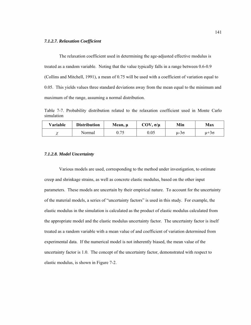
141
7.1.2.7. Relaxation Coefficient
The relaxation coefficient used in determining the age-adjusted effective modulus is
treated as a random variable. Noting that the value typically falls in a range between 0.6-0.9
(Collins and Mitchell, 1991), a mean of 0.75 will be used with a coefficient of variation equal to
0.05. This yields values three standard deviations away from the mean equal to the minimum and
maximum of the range, assuming a normal distribution.
Table 7-7. Probability distribution related to the relaxation coefficient used in Monte Carlo simulation
Variable Distribution Mean, μ COV, σ/μ Min Max
χ Normal 0.75 0.05 μ-3σ μ+3σ
7.1.2.8. Model Uncertainty
Various models are used, corresponding to the method under investigation, to estimate
creep and shrinkage strains, as well as concrete elastic modulus, based on the other input
parameters. These models are uncertain by their empirical nature. To account for the uncertainty
of the material models, a series of “uncertainty factors” is used in this study. For example, the
elastic modulus in the simulation is calculated as the product of elastic modulus calculated from
the appropriate model and the elastic modulus uncertainty factor. The uncertainty factor is itself
treated as a random variable with a mean value of and coefficient of variation determined from
experimental data. If the numerical model is not inherently biased, the mean value of the
uncertainty factor is 1.0. The concept of the uncertainty factor, demonstrated with respect to
elastic modulus, is shown in Figure 7-2.

142
Ela
stic
Mod
ulus
, E
c
Figure 7-2. Conceptual depiction of the method used to consider model uncertainty in the Monte Carlo simulation
The elastic modulus uncertainty factor distribution is determined based on the
experimental data summarized by Tadros et. al. (2003), as shown in Figure 7-3. The range of
compressive strengths from 5-12 ksi is identified as most common to North American bridge
construction, so the uncertainty factor distribution will be developed with respect to that range.
The approximate limits of the experimental data will be taken as two standard deviations away
from the mean value. The mean value of the uncertainty factor is assumed 1.0, meaning the
numerical model is not biased. The data points shown in Figure 7-3 suggest some bias in the
model, however, most of the data points beyond the limits indicated by the green outline are from
the same set of test specimens (represented by a triangle). This suggests there may have been
something unique about the test procedure or the concrete being tested. Furthermore, the data
points beyond the limits highlighted represent high elastic moduli. Ignoring these stiffer concrete
mixes in considering flexural analysis at service is conservative.

143
4σ =
400
0 ks
i
Figure 7-3. Determination of the model uncertainty factor for concrete elastic modulus (Data source: Tadros et. al., 2003)
The model uncertainty factor distribution will be defined for the middle of the range
indicated, f’c = 8.5 ksi. At this point, the numerical model estimates the elastic modulus to be
5600 ksi. The limits of the observed elastic modulus at f’c = 8.5 ksi are approximately 3400 ksi
and 7400 ksi. Taking these limits to be two standard deviations above and below the mean, the
coefficient of variation can be calculated as shown in (7-1).
10005600
0.18 (7-1)
Estimating model uncertainty factor distributions for creep and shrinkage is more
complex because the numerical models are based on many input factors. An approach similar to
that taken for elastic modulus is not reasonable because there are many dependent variables. ACI
209 (2008) compares the ACI 209-92 shrinkage and creep models with the RILEM databank. In

144
considering the ratio of measured-to-calculated values for shrinkage and creep strain, ACI 209-
(2008) reports a coefficient of variation of 0.41 for shrinkage and 0.30 for creep. Since the
AASHTO 2004 material model was shown to be similar to the ACI 209-92 model in Chapter 2,
the coefficients of variation shown in ACI 209-92 are adopted for this study. Also, these
parameters will be assumed applicable to the AASHTO 2005 model. The uncertainty factor
distributions are summarized in Table 7-8.
Table 7-8. Probability distributions related to the model uncertainty factors for concrete creep, shrinkage, and elastic modulus used in Monte Carlo simulation
Variable Distribution Mean, μ COV, σ/μ Min Max
εuncer Normal 1.0 0.41 μ-3σ μ+3σ
ψuncer Normal 1.0 0.30 μ-3σ μ+3σ
Ec-uncer Normal 1.0 0.18 μ-3σ μ+3σ
7.1.2.9. Applied Loads
The applied live load is not considered as part of the uncertainty analysis because it does
not affect the prestress loss. Girder selfweight, deck selfweight, and super-imposed dead load,
however, do affect prestress losses. Therefore, they will be treated as random variables. Normal
distributions and coefficients of variation matching those used to represent precast elements
(0.005) and cast-in-place construction (0.05) will be used for girder selfweight and deck
selfweight, respectively. Since the super-imposed dead load includes allowance for future
wearing surface, a higher coefficient of variation (0.2) will be assumed.

145
Table 7-9. Probability distributions related to applied loads used in Monte Carlo simulation
Variable Distribution Mean, μ COV, σ/μ Min Max
Mg Normal Nominal 0.005 μ-3σ μ+3σ
Md Normal Nominal 0.05 μ-3σ μ+3σ
MSIDL Normal Nominal 0.2 μ-3σ μ+3σ
7.1.3. Uncertainty Study Results
The parameters of the PCI BDM Example 9.4 (1997) bridge are used as a starting point
for the uncertainty study by Monte Carlo simulation. The input parameter distributions presented
in Section 7.1.2 are used, and 10,000 simulation cycles are run. A histogram of the results for
each method of estimating prestress losses is shown in Figure 7-4. The seven methods considered
in the study can be summarized as follows:
AASHTO 2005 (AASHTO 2005): The AASHTO 2005 prestress loss method is
used in conjunction with the AASHTO 2005 concrete material property model.
AASHTO 2005 (AASHTO 2004): The AASHTO 2005 prestress loss method is
used in conjunction with the AASHTO 2004 concrete material property model.
AASHTO 2005, simplified: The simplified prestress loss method of AASHTO
2005 is used. The AASHTO 2005 material property model is inherent.
AASHTO 2004: The AASHTO 2004 prestress loss method is used. The
AASHTO 2004 material property model is inherent.
Time Step (AASHTO 2005): The time step method is used with the AASHTO
2005 material property model.
Time Step (AASHTO 2004): The time step method is used with the AASHTO
2004 material property model

146
Direct Method: The Direct Method is used to estimate prestress losses. The
AASHTO 2005 material property model is inherent.
Figure 7-4. Histogram of Monte Carlo simulation results for prestress loss estimates applied to PCI BDM Example 9.4
The parameters of the simulation output distributions for prestress loss are summarized in
Table 7-10.
The mean values of the simulated distribution and the nominal results, calculated based
on nominal input values, are graphed in Figure 7-5.
0
0.05
0.1
0.15
0.2
0.25
0.3
0.35
20 30 40 50 60 70 80
Fre
qu
en
cy
Prestress Loss (ksi)
AASHTO 2005 (AASHTO 2005)
AASHTO 2005 (AASHTO 2004)
AASHTO 2005, simplif ied
AASHTO 2004
Time Step (AASHTO 2005)
Time Step (AASHTO 2004)
P/S Loss Method (Creep/Shrinkage Model)
Direct Method

147
Table 7-10. Summary of Monte Carlo simulation results for prestress loss estimates applied to PCI BDM Example 9.4
Method Mean (ksi) Standard Deviation (ksi)
AASHTO 2005 (AASHTO 2005) 44.6 7.3
AASHTO 2005 (AASHTO 2004) 46.5 7.2
AASHTO 2005, simplified 44.4 4.8
AASHTO 2004 56.6 2.9
Time Step (AASHTO 2005) 44.1 7.8
Time Step (AASHTO 2004) 46.0 7.7
Direct Method 45.2 7.4
Figure 7-5. Comparison of mean values from Monte Carlo simulation frequency distribution with nominal design values for prestress loss applied to PCI BDM Example 9.4
0 10 20 30 40 50 60
AASHTO 2005 (AASHTO 2005)
AASHTO 2005 (AASHTO 2004)
AASHTO 2005, Simplified
AASHTO 2004
Time Step (AASHTO 2005)
Time Step (AASHTO 2004)
Direct Method
Prestress Loss (ksi)
Mean of Frequency Distribution Nominal (Design) ValuesLoss Method (CR/SH Model)
Pro
po
sed
Bas
elin
eA
AS
HT
O M
eth
od
s

148
Figure 7-4 and Table 7-10 show that the AASHTO 2005 method, the time step method,
and the Direct Method produce results with a similar mean and standard deviation, regardless of
the material property model chosen. The AASHTO 2005 simplified method has a mean value
close to that of the other methods, but a smaller standard deviation. The AASHTO 2004 method
has a higher mean and smaller standard deviation than the other methods. This analysis suggests
that the Direct Method produces accurate results and that all simplifications made during its
development were reasonable. The comparison in Figure 7-5 shows that in all cases except for
the AASHTO 2004 method the nominal value calculation is conservative. Much of the
conservatism results from the truncated distribution for concrete compression strength, f’c.
Figure 7-6 shows results from the same analysis as Figure 7-4, with respect to extreme
bottom fiber concrete stress, as predicted by each method. The parameters of the simulation
output distributions for prestress loss are summarized in Table 7-11. The mean values of the
simulated distribution and the nominal results, calculated based on nominal input values, are
graphed in Figure 7-7.
The horizontal scale in Figures 7-5 and 7-7 can be misleading. The zero point represents
the division between tension and compression, but is not an absolute zero. Therefore, the values
should not be compared in terms of percentage difference. To make the results meaningful, it
should be noted that each additional prestressing strand in the girder would contribute
approximately 0.06 ksi of additional compression at the bottom fiber. The horizontal axis in
Figure 7-7 is formatted so that each gridline represents the contribution of each prestressing
strand. Figure 7-7 shows that the nominal result of each method is conservative relative to the
mean of the simulation data. Even more importantly, the nominal mean value calculated by the
Direct Method is conservative compared with the mean value of the Monte Carlo simulation
results for the time step method, regardless of the material property model chosen.

149
Figure 7-6. Histogram of Monte Carlo simulation results for bottom fiber concrete stress estimates applied to PCI BDM Example 9.4
Table 7-11. Summary of Monte Carlo simulation results for prestress loss estimates applied to PCI BDM Example 9.4
Method Mean (ksi) Standard Deviation (ksi)
AASHTO 2005 (AASHTO 2005) 0.41 0.20
AASHTO 2005 (AASHTO 2004) 0.35 0.20
AASHTO 2005, simplified 0.14 0.12
AASHTO 2004 0.40 0.10
Time Step (AASHTO 2005) 0.26 0.18
Time Step (AASHTO 2004) 0.23 0.21
Direct Method 0.35 0.14
0
0.05
0.1
0.15
0.2
0.25
0.3
0.35
‐0.5 ‐0.4 ‐0.3 ‐0.2 ‐0.1 0 0.1 0.2 0.3 0.4 0.5 0.6 0.7 0.8 0.9 1 1.1 1.2 1.3 1.4 1.5
Fre
qu
en
cy
Bottom Fiber Concrete Stress (ksi) [Positive Indicates Tension]
AASHTO 2005 (AASHTO 2005)
AASHTO 2005 (AASHTO 2004)
AASHTO 2005, simplif ied
AASHTO 2004
Time Step (AASHTO 2005)
Time Step (AASHTO 2004)
P/S Loss Method (Creep/Shrinkage Model)
Direct Method

150
Figure 7-7. Comparison of mean values from Monte Carlo simulation frequency distribution with nominal design values for prestress loss applied to PCI BDM Example 9.4
It can also be seen that, even though the AASHTO 2005 simplified method provides a reasonable
estimate of losses, it is unconservative for extreme fiber stresses.
The FHWA (Wassef et. al., 2003) example bridge (presented in Section 5.2.2) is used for
a separate baseline study. This bridge is chosen because the initial prestressing is much less – the
precompression of the extreme bottom fiber is approximately 2/3 of that in the PCI BDM
example – so a different type of design can be evaluated. A histogram of the results for each
method of estimating prestress losses is shown in Figure 7-4.
The parameters of the simulation output distributions for prestress loss are summarized in
Table 7-12.
0 0.06 0.12 0.18 0.24 0.3 0.36 0.42 0.48 0.54 0.6
AASHTO 2005 (AASHTO 2005)
AASHTO 2005 (AASHTO 2004)
AASHTO 2005, Simplified
AASHTO 2004
Time Step (AASHTO 2005)
Time Step (AASHTO 2004)
Direct Method
Bottom Fiber Concrete Stress (ksi) [Positive Indicates Tension]
Mean of Frequency Distribution Nominal (Design) ValuesLoss Method (CR/SH Model)
Pro
po
sed
Bas
elin
eA
AS
HT
O M
eth
od
s

151
Figure 7-8. Histogram of Monte Carlo simulation results for prestress loss estimates applied to the FHWA example
Table 7-12. Summary of Monte Carlo simulation results for prestress loss estimates applied to the FHWA Example
Method Mean (ksi) Standard Deviation (ksi)
AASHTO 2005 (AASHTO 2005) 34.5 6.4
AASHTO 2005 (AASHTO 2004) 34.5 6.1
AASHTO 2005, simplified 35.0 3.9
AASHTO 2004 41.4 2.5
Time Step (AASHTO 2005) 37.4 7.2
Time Step (AASHTO 2004) 37.0 6.9
Direct Method 35.1 5.9
The mean values of the simulated distribution and the nominal results, calculated based
on nominal input values, are graphed in Figure 7-9.
0
0.05
0.1
0.15
0.2
0.25
0.3
0.35
20 30 40 50 60 70 80
Fre
qu
en
cy
Prestress Loss (ksi)
AASHTO 2005 (AASHTO 2005)
AASHTO 2005 (AASHTO 2004)
AASHTO 2005, simplif ied
AASHTO 2004
Time Step (AASHTO 2005)
Time Step (AASHTO 2004)
P/S Loss Method (Creep/Shrinkage Model)
Direct Method

152
Figure 7-9. Comparison of mean values from Monte Carlo simulation frequency distribution with nominal design values for prestress loss applied to the FHWA Example
As with the PCI BDM example bridge, the FHWA example shows in Figure 7-8 and
Table 7-12 that the AASHTO 2005 method, the time step method, and the Direct Method produce
results with a similar mean and standard deviation, regardless of the material property model
chosen. The AASHTO 2005 simplified method has a mean value close to that of the other
methods, but a smaller standard deviation. The AASHTO 2004 method has a higher mean and
smaller standard devation than the other methods. This analysis suggests that the Direct Method
produces accurate results and that all simplifications made during its development were
reasonable. The comparison in Figure 7-9 shows that in all cases the nominal value calculation is
conservative. Much of the conservatism results from the truncated distribution for concrete
compression strength, f’c.
0 10 20 30 40 50 60
AASHTO 2005 (AASHTO 2005)
AASHTO 2005 (AASHTO 2004)
AASHTO 2005, Simplified
AASHTO 2004
Time Step (AASHTO 2005)
Time Step (AASHTO 2004)
Direct Method
Prestress Loss (ksi)
Mean of Frequency Distribution Nominal (Design) ValuesLoss Method (CR/SH Model)
Pro
po
sed
Bas
elin
eA
AS
HT
O M
eth
od
s

153
Figure 7-10 shows results from the same analysis as Figure 7-8, with respect to extreme
bottom fiber concrete stress, as predicted by each method.
Figure 7-10. Histogram of Monte Carlo simulation results for bottom fiber concrete stress estimates applied to the FHWA example
The parameters of the simulation output distributions for prestress loss are summarized in
Table 7-13. The mean values of the simulated distribution and the nominal results, calculated
based on nominal input values, are graphed in Figure 7-11.
0
0.05
0.1
0.15
0.2
0.25
0.3
0.35
‐0.5 ‐0.4 ‐0.3 ‐0.2 ‐0.1 0 0.1 0.2 0.3 0.4 0.5 0.6 0.7 0.8 0.9 1 1.1 1.2 1.3 1.4 1.5
Fre
qu
en
cy
Bottom Fiber Concrete Stress (ksi) [Positive Indicates Tension]
AASHTO 2005 (AASHTO 2005)
AASHTO 2005 (AASHTO 2004)
AASHTO 2005, simplif ied
AASHTO 2004
Time Step (AASHTO 2005)
Time Step (AASHTO 2004)
P/S Loss Method (Creep/Shrinkage Model)
Direct Method
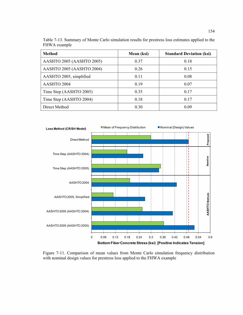
154
Table 7-13. Summary of Monte Carlo simulation results for prestress loss estimates applied to the FHWA example
Method Mean (ksi) Standard Deviation (ksi)
AASHTO 2005 (AASHTO 2005) 0.37 0.18
AASHTO 2005 (AASHTO 2004) 0.26 0.15
AASHTO 2005, simplified 0.11 0.08
AASHTO 2004 0.19 0.07
Time Step (AASHTO 2005) 0.35 0.17
Time Step (AASHTO 2004) 0.18 0.17
Direct Method 0.30 0.09
Figure 7-11. Comparison of mean values from Monte Carlo simulation frequency distribution with nominal design values for prestress loss applied to the FHWA example
0 0.06 0.12 0.18 0.24 0.3 0.36 0.42 0.48 0.54 0.6
AASHTO 2005 (AASHTO 2005)
AASHTO 2005 (AASHTO 2004)
AASHTO 2005, Simplified
AASHTO 2004
Time Step (AASHTO 2005)
Time Step (AASHTO 2004)
Direct Method
Bottom Fiber Concrete Stress (ksi) [Positive Indicates Tension]
Mean of Frequency Distribution Nominal (Design) ValuesLoss Method (CR/SH Model)
Pro
po
sed
Bas
elin
eA
AS
HT
O M
eth
od
s

155
Figure 7-11 shows that the nominal result of each method is conservative relative to the
mean of the simulation data, except for the time step method using the AASHTO 2005 material
property model. Even more importantly, the nominal mean value calculated by the Direct
Method is conservative compared with the mean value of the Monte Carlo simulation results for
the time step method, regardless of the material property model chosen.
7.1.4. Irreversible Creep
The concept of irreversible creep is introduced in Section 5.5. In that section, using
results from the time step method, it is shown that incomplete creep recovery leads to larger
prestress losses and larger extreme fiber tension stresses than calculated when full creep recovery
is assumed.
To further study the effect of irreversible creep, the Monte Carlo simulation of the PCI
BDM Example 9.4 bridge is run treating the creep recovery factor as a random variable. In this
case, the creep recovery factor is assumed to have a uniform distribution ranging from 50% to
100%. A histogram of the Monte Carlo simulation results for prestress losses is shown in Figure
7-12.
Only the time step method is affected by the creep recovery factor. It can be seen in
Figure 7-12, relative to Figure 7-4, that the blue lines representing the time step method results
moved slightly towards the higher end of the range. The mean values of the distributions are
compared in Figure 7-13, along with the results of calculations using nominal values. A small
increase in the mean value of the time step method results is apparent, compared with Figure 7-5.
The bottom fiber stress estimates from the same simulation shown in Figures 7-12 and 7-
13 are shown in terms of a histogram of results (Figure 7-14) and a comparison of simulation
mean and nominal values (Figure 7-15).
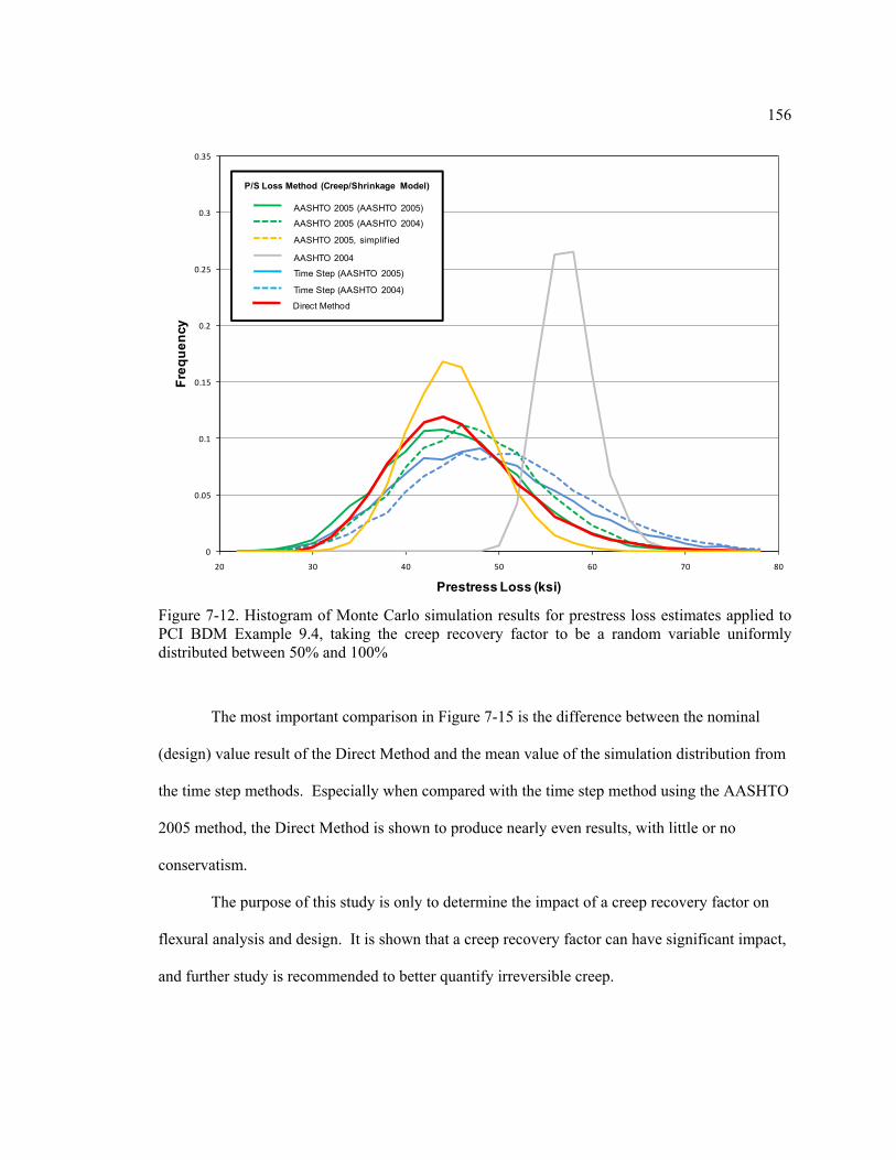
156
Figure 7-12. Histogram of Monte Carlo simulation results for prestress loss estimates applied to PCI BDM Example 9.4, taking the creep recovery factor to be a random variable uniformly distributed between 50% and 100%
The most important comparison in Figure 7-15 is the difference between the nominal
(design) value result of the Direct Method and the mean value of the simulation distribution from
the time step methods. Especially when compared with the time step method using the AASHTO
2005 method, the Direct Method is shown to produce nearly even results, with little or no
conservatism.
The purpose of this study is only to determine the impact of a creep recovery factor on
flexural analysis and design. It is shown that a creep recovery factor can have significant impact,
and further study is recommended to better quantify irreversible creep.
0
0.05
0.1
0.15
0.2
0.25
0.3
0.35
20 30 40 50 60 70 80
Fre
qu
en
cy
Prestress Loss (ksi)
AASHTO 2005 (AASHTO 2005)
AASHTO 2005 (AASHTO 2004)
AASHTO 2005, simplif ied
AASHTO 2004
Time Step (AASHTO 2005)
Time Step (AASHTO 2004)
P/S Loss Method (Creep/Shrinkage Model)
Direct Method

157
Figure 7-13. Comparison of mean values from Monte Carlo simulation frequency distribution with nominal design values for prestress loss applied to PCI BDM Example 9.4, taking the creep recovery factor as a random variable uniformly distributed between 50% and 100%
7.2. Sensitivity Study
The sensitivity of the results to certain input variables is evaluated graphically in this
section based on plots of the Monte Carlo simulation data. The base input variable is plotted on
the x-axis, while the output (prestress loss or bottom fiber stress) is plotted on the y-axis. For the
sake of convenient comparison, output from both the time step solution (using the AASHTO
2005 material property model) and the Direct Method will be plotted on the same graph. A linear
trend line is included only to aid in the visual comparison. The relative slope of this line between
the two methods is perhaps the most important result. A zero-slope line (horizontal) suggests that
knowledge of the input value provides no useful information about the resulting output. Steeper
0 10 20 30 40 50 60
AASHTO 2005 (AASHTO 2005)
AASHTO 2005 (AASHTO 2004)
AASHTO 2005, Simplified
AASHTO 2004
Time Step (AASHTO 2005)
Time Step (AASHTO 2004)
Direct Method
Prestress Loss (ksi)
Mean of Frequency Distribution Nominal (Design) ValuesLoss Method (CR/SH Model)
Pro
po
sed
Bas
elin
eA
AS
HT
O M
eth
od
s

158
Figure 7-14. Histogram of Monte Carlo simulation results for bottom fiber stress estimates applied to PCI BDM Example 9.4, taking the creep recovery factor to be a random variable uniformly distributed between 50% and 100%
slopes suggest stronger dependence on the input. Note that not all input values are explicitly
considered in the Direct Method. Ideally, only variables demonstrating little significance in the
time step method will be removed when simplifying calculations to develop the Direct Method.
The primary input variables remaining in the Direct Method are relative humidity, girder
concrete strength, deck concrete strength, and steel elastic modulus. Those variables are
examined first to verify that they exhibit similar influence on both the Time Step and Direct
Method results. “Similar influence” is defined loosely to mean that the two sets of data have
similar slopes in their trend. A vertical offset between the methods cannot necessarily be
attributed to the variable under study. Additionally, plots are provided for time at deck placement
0
0.05
0.1
0.15
0.2
0.25
0.3
0.35
‐0.5 ‐0.4 ‐0.3 ‐0.2 ‐0.1 0 0.1 0.2 0.3 0.4 0.5 0.6 0.7 0.8 0.9 1 1.1 1.2 1.3 1.4 1.5
Fre
qu
en
cy
Bottom Fiber Concrete Stress (ksi) [Positive Indicates Tension]
AASHTO 2005 (AASHTO 2005)
AASHTO 2005 (AASHTO 2004)
AASHTO 2005, simplif ied
AASHTO 2004
Time Step (AASHTO 2005)
Time Step (AASHTO 2004)
P/S Loss Method (Creep/Shrinkage Model)
Direct Method

159
Figure 7-15. Comparison of mean values from Monte Carlo simulation frequency distribution with nominal design values for bottom fiber stress applied to PCI BDM Example 9.4, taking the creep recovery factor as a random variable uniformly distributed between 50% and 100%
to further justify removal of this variable and combine the two time steps currently defined in the
code provisions. Results are provided in Figures 7-8 through 7-12. In each case it can be seen
that the slopes of the trendlines for the two methods are very similar. This suggests that the
sensitivity of the Direct Method to its primary input terms is appropriate. Also, removal of the td
factor is justified as no noticeable trend is seen in Figure 7-12.
0 0.06 0.12 0.18 0.24 0.3 0.36 0.42 0.48 0.54 0.6
AASHTO 2005 (AASHTO 2005)
AASHTO 2005 (AASHTO 2004)
AASHTO 2005, Simplified
AASHTO 2004
Time Step (AASHTO 2005)
Time Step (AASHTO 2004)
Direct Method
Bottom Fiber Concrete Stress (ksi) [Positive Indicates Tension]
Mean of Frequency Distribution Nominal (Design) ValuesLoss Method (CR/SH Model)
Pro
po
sed
Bas
elin
eA
AS
HT
O M
eth
od
s

160
0
10
20
30
40
50
60
70
0 10 20 30 40 50 60 70 80 90 100
Pre
dic
ted
Lo
ss
of
Pre
str
ess
(k
si)
Ambient Relative Humidity
Time Step (NCHRP 496)
Direct Method
‐0.4
‐0.2
0
0.2
0.4
0.6
0.8
1
0 10 20 30 40 50 60 70 80 90 100
Pre
dic
ted
Bo
tto
m F
ibe
r S
tre
ss
(k
si)
Ambient Relative Humidity
Time Step (NCHRP 496)
Direct Method
Figure 7-16. Scatter plot of Monte Carlo simulation results to indicate sensitivity to the relative humidity input

161
0
10
20
30
40
50
60
70
0 2 4 6 8 10 12
Pre
dic
ted
Lo
ss
of
Pre
str
ess
(k
si)
Girder Concrete Compressive Strength, f'c (ksi)
Time Step (NCHRP 496)
Direct Method
‐0.4
‐0.2
0
0.2
0.4
0.6
0.8
1
0 2 4 6 8 10 12
Pre
dic
ted
Bo
tto
m F
ibe
r S
tre
ss
(ks
i)
Girder Concrete Compressive Strength, f'c (ksi)
Time Step (NCHRP 496)
Direct Method
Figure 7-17. Scatter plot of Monte Carlo simulation results to indicate sensitivity to the girder compressive strength input

162
0
10
20
30
40
50
60
70
0 1 2 3 4 5 6 7
Pre
dic
ted
Lo
ss
of
pre
str
es
s (k
si)
Deck Concrete Compressive Strength, f'cd(ksi)
Time Step (NCHRP 496)
Direct Method
‐0.4
‐0.2
0
0.2
0.4
0.6
0.8
1
0 1 2 3 4 5 6 7
Pre
dic
ted
Bo
tto
m F
iber
Str
ess
(k
si)
Deck Concrete Compressive Strength, f'cd(ksi)
Time Step (NCHRP 496)
Direct Method
Figure 7-18. Scatter plot of Monte Carlo simulation results to indicate sensitivity to the deck compressive strength input

163
0
10
20
30
40
50
60
70
26500 27000 27500 28000 28500 29000 29500 30000 30500
Pre
dic
ted
Lo
ss
of
Pre
str
es
s (k
si)
Elastic Modulus of Prestressing Steel, Eps (ksi)
Time Step (NCHRP 496)
Direct Method
‐0.4
‐0.2
0
0.2
0.4
0.6
0.8
1
26500 27000 27500 28000 28500 29000 29500 30000 30500
Pre
dic
ted
Bo
tto
m F
ibe
r S
tre
ss
(ks
i)
Elastic Modulus of Prestressing Steel, Eps (ksi)
Time Step (NCHRP 496)
Direct Method
Figure 7-19. Scatter plot of Monte Carlo simulation results to indicate sensitivity to the elastic modulus of prestressing steel input

164
0
10
20
30
40
50
60
70
0 50 100 150 200 250 300 350 400
Pre
dic
ted
Lo
ss
of
Pre
str
ess
(k
si)
Time of Deck Placement, tdeck (days)
Time Step (NCHRP 496)
Direct Method
‐0.4
‐0.2
0
0.2
0.4
0.6
0.8
1
0 50 100 150 200 250 300 350 400
Pre
dic
ted
Bo
tto
m F
ibe
r S
tre
ss (
ksi
)
Time of Deck Placement, tdeck (days)
Time Step (NCHRP 496)
Direct Method
Figure 7-20. Scatter plot of Monte Carlo simulation results to indicate sensitivity to the time of deck placement input

165
Additionally, it is informative to compare small errors in estimating material properties
(on the order of 10-20% error) with errors of similar magnitude in commonplace (and seemingly
more predictable) variables. In a simple sensitivity study, the material property model errors for
elastic modulus, creep, and shrinkage are considered. Additionally, the variables related to deck
self-weight, live load, and relative humidity are included. The effect of errors +/- 20% from the
nominal value is reported in Figures 7-21 and 7-22 for prestress loss and bottom fiber stress,
respectively.
Figure 7-21. Sensitivity study comparing the effect on prestress loss of material property model errors with that of other common variables
40
42
44
46
48
50
52
54
56
58
60
0.7 0.8 0.9 1 1.1 1.2 1.3
Pre
str
es
s L
os
s (k
si)
Error in Input Value [>1 Indicates Value was Underestimated in Design]
E error (Elastic Modulus)
ε error (Shrinkage)
ψ error (Creep)
Moment Due to Deck Self-weight
Moment Due to Live Load
Relative Humidity

166
Figure 7-22. Sensitivity study comparing the effect on prestress loss of material property model errors with that of other common variables
These plots are quite helpful in putting the need for precise material property models into
perspective. Figure 7-22 is particularly important since the amount of prestressing is ultimately
determined by a bottom fiber stress check. Note that the vertical axis in Figure 7-22 has been
formatted to show a gridline at increments of 0.06 ksi. This is approximately the stress
contributed by each prestressing strand. In other words, for each gridline crossed another
prestressing strand would be needed – or could be removed. It is apparent from Figure 7-22 that
small errors in the calculation of load or estimating relative humidity are of greater significance in
the performance of the system than small errors in estimating material properties.
Two conclusions can be drawn from this simple analysis. First, it seems unnecessary for
the AASHTO 2005 method for estimating losses to remain open to use of any material property
0
0.06
0.12
0.18
0.24
0.3
0.36
0.42
0.48
0.54
0.6
0.66
0.72
0.7 0.8 0.9 1 1.1 1.2 1.3
Bo
tto
m F
ibe
r Co
nc
rete
Str
es
s (k
si)
Error in Input Value [>1 Indicates Value was Underestimated in Design]
E error (Elastic Modulus)
ε error (Shrinkage)
ψ error (Creep)
Moment Due to Deck Self-weight
Moment Due to Live Load
Relative Humidity
167
model. This flexibility prevents algebraic simplification of the method and renders a more
mathematically complex method for designers. Secondly, and following the first conclusion, the
adoption of the AASHTO 2005 material property model in the Direct Method is justified. The
choice of material model for use in the Direct Method would be of little consequence.
7.3. Summary
Several important observations are made from the uncertainty and sensitivity studies:
The uncertainty distributions for the time step, AASHTO 2005, and Direct
Method are similar for both prestress loss and bottom fiber stress estimates. This
suggests that the variables removed in simplifying the predictive method had
little impact on the total uncertainty. The AASHTO 2004 method shows a much
smaller standard deviation, indicating that significant variables were removed in
developing that method, handicapping the accuracy of the results and suggesting
a more precise result than realistically possible.
Bottom fiber stresses cannot be known accurately with only an estimate of
prestress losses. This is especially evident in the FHWA design example, in
which the AASHTO 2004 method predicts the highest prestress losses of any
method, but predicts much less bottom fiber tension. This happens because the
AASHTO 2004 approach estimates prestress losses only; the other methods also
consider differential shrinkage between the deck and the girder. Therefore, the
assumption that the AASHTO 2005 method is less conservative than the
AASHTO 2004 method is not entirely true. The methods should be compared
with respect to bottom fiber stress estimates.
168
In each case the nominal result of the Direct Method was conservative (larger
prestress loss and/or larger bottom fiber tension) relative to the mean value of the
uncertainty distribution for the Direct Method. More importantly, the nominal
result of the Direct Method compares evenly or conservatively with the mean
value of the uncertainty distribution relative to the time step method, regardless
of the material property model assumed. The conservative nature of the nominal
results compared with the uncertainty distributions can be attributed largely to
the fact that concrete strengths typically exceed design target values by a
significant amount, while not often falling short of the design value.
The Direct Method yields results with similar accuracy and uncertainty as the
AASHTO 2005 method.
The choice of material property model to be used in the prediction of prestress
losses and bottom fiber stresses is of less consequence than suggested by the
development of a new model for high strength concrete in AASHTO 2005. It
should also be noted that the AASHTO 2005 method will estimate much higher
bottom fiber tension stresses in cases where concrete strength in the girder is
substantially higher than that of the deck. The examples in this section had
relatively small gradients between the deck and the girder.
The sensitivity study indicates that the response of each input variable in the
Direct Method matches its response in the time step method. Also, the sensitivity
study further justifies removal of the time-of-deck-placement variable.

Chapter 8
Summary and Conclusions
This thesis documents research related to the time-dependent behavior of pretensioned
concrete bridge girders. The recommendations of NCHRP Report 496 that were adopted in the
AASHTO 2005 method for quantifying concrete material properties and estimating prestress
losses were developed in response to the need for a method more applicable to high strength
concrete. The resulting specifications are more elaborate than their predecessor, AASHTO 2004,
and seemingly less conservative because smaller prestress losses were predicted. This study
examines both the AASHTO 2004 and AASHTO 2005 methods, along with the Canadian S6-06
method, and proposes a simplified approach called the Direct Method. The Direct Method is
derived from fundamental principles and incorporates the AASHTO 2005 material property
model. An uncertainty study considers the variability of input parameters in predicting time-
dependent behavior of concrete girders and justifies the Direct Method as a suitable simplified
analysis approach.
8.1. Conclusions
Major conclusions and observations of this research program can be summarized as
follows:
The concrete material property models and simplified approaches to prestress
loss estimates common in North American bridge design practice are
summarized and compared.

170
A detailed review of NCHRP Report 496, which documents the material property
model and prestress loss method adopted into AASHTO 2005, is included as
part of the discussion in Chapters 2 and 3. Questions, concerns, and observations
about changes introduced in AASHTO 2005, relative to previous versions of the
specifications, include:
o The shrinkage data from the experimental work done as part of the
NCHRP Report 496 research is not consistent with expectations.
Additional research is needed to validate the shrinkage model developed
from this experimentation.
o The AASHTO 2005 method introduces a strength correction factor in the
concrete shrinkage model. In the AASHTO 2004 model, the strength
correction factor was only applied to creep. The experimental data used
to develop the AASHTO 2005 method does not justify the strength
correction factor. The strength correction factor has a significant impact
on time-dependent analysis because it increases the effective force
considered due to differential shrinkage in cases where the girder and
composite deck have different concrete strengths.
o In the absence of data specific to the aggregate source, the equation for
estimating the concrete elastic modulus by AASHTO 2005 is identical to
that used in AASHTO 2004.
o The AASHTO 2005 method divides time-dependent behavior into stages
before and after deck placement. A sensitivity study of the AASHTO
2005 model and results from the time step method justify combining the
stages for simplified analysis.

171
o AASHTO 2005 introduces a transformed section coefficient to model the
restraint of bonded prestressing against creep and shrinkage of concrete.
The coefficient varies over a small range and can be taken as 0.9 for
shrinkage effects and 0.85 for creep effects.
o Differential shrinkage is considered in AASHTO 2005 in terms of an
elastic prestressing gain. Since this language can create confusion, the
Direct Method proposes modeling differential shrinkage by an effective
force at the centroid of the deck.
A time step approach is used as a baseline for the comparison of prestress loss
methods and material property models. Analysis of the time step routine results
verify that prestress losses and extreme fiber concrete stresses cannot be directly
correlated. The complex interaction of elastic and inelastic strains must be
considered in flexural design for service.
A simple, complete example problem to demonstrate use of the time step method
is provided in Appendix B.
The Direct Method is developed as a simple procedure for time-dependent
analysis derived from basic principles of mechanics. The format of the method is
familiar to most designers because it is modeled after the AASHTO 2004
method. The inclusion of the AASHTO 2005 material model for high strength
concrete and the addition of a differential shrinkage term makes the method more
complete than the AASHTO 2004 model.
Monte Carlo simulation results suggest that the Direct Method, AASHTO 2005
method, and time step method all have similar means and variation in estimating
prestress losses and extreme fiber stresses when the uncertainty of the input
variables is considered. Observations specific to the uncertainty study include:

172
o Comparison of simulation results for the time step method using the
AASHTO 2005 material model and that using the AASHTO 2004
material model are similar, suggesting that the choice of material
property model used in flexural design is not significant.
o In all simulation cases studied the nominal Direct Method results
compared closely or conservatively with the simulated values that
considered the underlying uncertainty of the method.
The Direct Method is formatted into language suitable for inclusion in the
AASHTO LRFD Bridge Design Specifications, as shown in Appendix A.
An example problem demonstrating application of the Direct Method is provided
in Section 6.6.
Two specific needs for future research are identified and discussed in Section 8.2.
8.2. Future Research
This study has identified two needs for future research:
Irreversible creep impacts prestress loss and extreme fiber concrete stress.
Historically, methods in design specifications have assumed full creep recovery
in their development. Such an assumption is also made in the Direct Method.
Further research is needed to examine the effects of incomplete creep recovery.
An analysis by the time step method suggests that a creep recovery of 75% or
less would have significant impact on flexural design. A creep recovery factor,
or a creep recovery function, should be developed and recommended for the
stress analysis of pretensioned girders.

173
Considerations for differential shrinkage are new to the AASHTO Specifications,
first introduced in the 2005 Interim Revisions. The time step analysis in this
thesis verifies that differential shrinkage has significant impact on extreme fiber
concrete stresses. The area of the deck that acts compositely with the girder for
differential shrinkage calculations should be investigated. In the absence of
better information, the effective width calculation that represents the shear lag
effect in flexural analysis has been used. Experimental verification, or
improvement, of this assumption is needed.
8.3. Recommendations
The Direct Method is proposed as a simplified alternative to the AASHTO 2005 method
for time-dependent analysis of pretensioned girders. The Direct Method will be presented to T-
10, the technical committee within AASHTO dealing with concrete structures, in a format
suitable for inclusion in the AASHTO LRFD Bridge Design Specifications.

174
References
ACI Committee 209. (1992). “Prediction of Creep, Shrinkage, and Temperature Effects in Concrete Structures.” Committee Report, American Concrete Institute. Detroit, MI.
ACI Committee 209. (2008). “Guide for Modeling and Calculating Shrinkage and Creep in Hardened Concrete.” Committee Report, American Concrete Institute. Detroit, MI.
ACI Committee 363. (1992). “State of the Art Report on High-Strength Concrete.” Committee Report, American Concrete Institute. Detroit, MI.
Al-Omaishi, N., Tadros, M.K., and Seguirant, S.J. (2009). “Estimating Prestress Loss in Pretensioned High-Strength Concrete Members.” PCI Journal, 54(4), 132-159.
American Association of State Highway and Transportation Officials (AASHTO). (2004). “AASHTO LRFD Bridge Design Specifications.” Third Edition, Washington, DC.
American Association of State Highway and Transportation Officials (AASHTO). (2005). “AASHTO LRFD Bridge Design Specifications.” Third Edition including 2005 interim revisions, Washington, DC.
Barker, R.M., and Puckett, J.A. (1997). “Design of Highway Bridges: Based on the AASHTO LRFD Bridge Design Specifications.” John Wiley and Sons, Inc., New York, NY.
Barker, R.M., and Puckett, J.A. (2007). “Design of Highway Bridges: An LRFD Approach.” Second Edition. John Wiley and Sons, Inc, Hoboken, NJ.
Bazant, Z.P. (1972). “Prediction of Concrete Creep Effect Using Age-Adjusted Effective Modulus Method.” ACI Journal. 69(20). 212-217.
Canadian Standards Association (CSA). (2006). “Canadian Highway Bridge Design Code.” CAN/CSA S6-06.
Collins, M.P., and Mitchell, D. (1991). “Prestressed Concrete Structures.” Prentice-Hall, Inc, Englewood Cliffs, NJ.
Cousins, T. (2005). “Investigation of Long-term Prestress Losses in Pretensioned High Performance Concrete Girders.” Virginia Transportation Research Council, Report 05-CR20.
Cullen, A.C. and Frey, H.C. (1999). “Probabilistic Techniques in Exposure Assessment: A Handbook for Dealing with Variability and Uncertainty in Models and Inputs.” Plenum Press.

175
Dilger, W.H. (1982). “Creep Analysis of Prestressed Concrete Structures Using Creep Transformed Section Properties.” PCI Journal. 27(1). 89-117.
Grouni, H.N. (1973). “Prestressed Concrete – A Simplified Method for Loss Calculation.” ACI Journal. 70(2). 108-114.
Grouni. H.N. (1978). “Loss of Prestress Due to Relaxation After Transfer.” ACI Journal. 75(2). 64-66.
Hennessey, S.A. and Tadros, M.K. (2002). “Significance of Transformed Section Properties in Analysis for Required Prestressing.” PCI Journal. 47(6). 104-107.
Lin, T.Y. and Burns, N.H. (1981). “Design of Prestressed Concrete Structures.” Third Edition. John Wiley and Sons, Inc. New York, NY.
Magura, D.D., Sozen, M.A., and Siess, C.P. (1964). “A Study of Stress Relaxation in Prestressing Reinforcement.” PCI Journal. 9(2). 13-57.
Mehta, P.K. and Monteiro, P.J.M. (2006). “Concrete: Microstructure, Properties, and Materials.” Third Edition. Mcgraw-Hill, New York, NY.
Mindess, S.J., Young, F.J., Darwin, D. (2002). “Concrete.” Second Edition. Pearson, Upper Saddle River, NJ.
Myers, J.J. and Carrasquillo, R.L. (1999). “Production and Quality Control of High Performance Concrete in Texas Bridge Structures.” Center for Transportation Research, Report 580/589-1. University of Texas. Austin, TX.
Precast/Prestressed Concrete Institute (PCI). (1997). “Precast/Prestressed Concrete Bridge Design Manual.” Precast/Prestressed Concrete Institute, Chicago, IL.
PCI Committee on Prestress Losses. (1975). “Recommendations for Estimating Prestress Losses.” PCI Journal, 20(4). 43-75.
Rizkalla, S., Mirmiran, K. Zia, P., Russell, H., and Mast, R. (2007). “Application of the LRFD Bridge Design Specifications to High-Strength Structural Concrete: Flexure and Compression Provisions.” NCHRP Report 595. Transportation Research Board, Washington, DC.
Tadros, M.K., Ghali, A., and Dilger, W.H. (1977). “Time-Dependent Analysis of Composite Frames.” ASCE Journal of Structural Engineering. 103(4). 871-884.
Tadros, M.K., Al-Omaishi, N., Seguirant, S.J., and Gallt, J.G. (2003). “Prestress Losses in Pretensioned High Strength Concrete Bridge Girders.” NCHRP Report 496. Transportation Research Board, Washington, DC.
Trost, H. (1967). “Implications of the Superposition Principle in Creep and Relaxation Problems for Concrete and Prestressed Concrete.” Beton-und Stahlbetonbau. Berlin-Wilmersdorf. No. 10. 230-238, 261-269. (in German).

176
Walton, S., and Bradberry, T. (2004). “Comparison of Methods for Estimating Prestress Losses for Bridge Girders.” Proceedings, Texas Section ASCE Fall Meeting, Sept 29-Aug 2. Houston, TX.
Wassef, W.G., Smith, C., Clancy, C.M., and Smith, M.J. (2003). “Comprehensive Design Example for Prestressed Concrete Girder Superstructure Bridge with Commentary.” Federal Highway Administration. Arlington, VA.
Wight, J.K. and Macgregor, J.G. (2009). “Reinforced Concrete – Mechanics and Design.” Fifth Edition. Pearson, Upper Saddle River, NJ.
Yue, L.L. and Taerwe, L. (1993). “Two-Function Method for the Prediction of Concrete Creep Under Decreasing Stress.” Materiaux et constructions. 26(159). 268-273.
Zia, P., Preston, H.K., Scott, N.L., and Workman, E.B. (1979). “Estimating Prestress Losses.” Concrete International. 1(2). 32-38.

177
Appendix A
Proposed Provision for the AASHTO LRFD Bridge Design Specifications
[Insert Article 5.9.5.5. Renumber current Article 5.9.5.5. as Article 5.9.5.6.] 5.9.5.5. Direct Method for Time-Dependent Analysis
5.9.5.5.1. General For pretensioned members the provisions of this article may be used in lieu of those provided in Articles 5.9.5.3 and 5.9.5.4. In the case of a precast girder with a composite cast-in-place deck, the effect of differential shrinkage between the components shall be considered in accordance with Article 5.9.5.4.2. This article shall apply in cases of normal-weight concrete and concrete compressive strength at transfer exceeding 3.5 ksi. For lightweight concrete, loss of prestress shall be based on the representative properties of the concrete to be used. The change in prestressing steel stress due to time-dependent loss, Δ , shall be determined as follows:
Δ Δ Δ Δ 5.9.5.5.1‐1
Prestress loss due to shrinkage of girder concrete (ksi)
Prestress loss due to creep of girder concrete (ksi)
Prestress loss due to relaxation of prestressing strands (ksi)
5.9.5.5.2. Loss of Prestress 5.9.5.5.2a Shrinkage Loss of prestress, in ksi, due to shrinkage may be taken as:
Δ
1401.3 ′ 3.8 10 5.9.5.5.2a‐1
The average annual ambient relative humidity (percent)
Design compressive strength of the girder concrete (ksi)
Elastic modulus of prestressing steel (ksi)
5.9.5.5.2b Creep

178
Loss of prestress, in ksi, due to creep may be taken as:
Δ 0.04
1951.3 ′ 2 Δ Δ 0 5.9.5.5.2b‐1
The stress, in ksi, at the centroid of the prestressing just after transfer; compression is indicated with a negative sign
Δ The stress change, in ksi, at the centroid of the prestressing due to application of deck weight and other permanent loads; a tension stress increment is indicated with a positive sign
Δ The stress change, in ksi, at the centroid of the prestressing due to shrinkage and relaxation losses, and differential shrinkage between the deck and girder; a tension stress increment is indicated with a positive sign.
Estimated elastic modulus of girder concrete in service
5.9.5.5.2c Relaxation of Prestressing Strands During the period from transfer to final time, the relaxation loss, Δ , may be taken equal to 2.5 ksi for low-relaxation strands where the stress in the strand at transfer exceeds 0.55fpy. In other cases, the relaxation loss can be neglected. 5.9.5.5.3. Shrinkage of Deck Concrete In the case of a cast-in-place deck made composite with a precast girder, the effect of differential shrinkage between the two components shall be considered. The effect may be modeled as a force applied to the full composite section at the level of the deck centroid. The force, in kips, may be taken as:
1 0.7 , 5.9.5.5.3‐1
An effective force, in kips, representing the effect of differential shrinkage between a cast-in-place deck and a precast girder in composite construction. A positive result shall be applied as a compression force on the composite section at the location of the deck centroid.
Differential shrinkage between the deck and the girder
Elastic modulus of deck concrete
Effective area of the deck
, Creep coefficient for deck concrete at final time due to stresses induced at the time of deck placement

179
Alternatively, the effective force at the centroid of the deck may be approximated by:
1.2 10
140 51
1
17 1951.3
5.9.5.5.3‐2
Average ambient relative humidity, %
Design compressive concrete strength for the deck, ksi
Design compressive concrete strength for the girder, ksi

180
Appendix B
Example of the Time Step Method
The following simple example is offered to demonstrate the time-step method. A 8”x12”
girder spans 16 feet simply-supported. It is prestressed with two ½” strands. A representative
deck is cast when the girder concrete age is 30 days. For the purposes of analysis, the deck
weight will be considered starting on day 30 and the deck stiffness will be considered on day 31.
This represents the case of unshored construction where the self-weight of the deck is carried by
the non-composite girder section. A constant temperature of 70 degrees will be assumed at all
time steps. The creep and shrinkage functions published in NCHRP 496 will be used to model
concrete behavior.
Aps Area of prestressing steel 0.306 in2
Ep Elastic modulus of prestressing steel 28500 ksi
dp Location of prestressing C.G., measured from top of deck 13 in
fJ Jacking stress 202.5 ksi
Ag Girder gross area 96 in2
Ig Girder gross moment of inertia 1152 in4
MSW Moment due to girder self-weight 38.4 k-in
MD Moment due to deck self-weight 25.6 k-in
MSIDL Moment due to superimposed dead load 20 k-in
MLL Moment due to live load 86 k-in
f’c Girder concrete is assumed 6 ksi at day 1 and increases linearly to 8 ksi at day 28
f’cd Deck concrete is assumed 3.2 ksi at day 1 and increases linearly to 4 ksi at day 28
The cross-section to be evaluated is shown in the figure below.

181
Time Step 1 (1 Day)
For the first time step, the effects of creep and shrinkage are ignored. Only the elastic
effect will be considered. The total strain and curvature on the cross-section can be found by
solving the simultaneous equations presented in the development of the time-step method. Each
of the constants must be determined before the equations can be solved.
Constant “A”
The modulus of elasticity of concrete, Ec, is taken to be 4415 ksi during step 1. The
constant A can be determined as follows (remember, the deck concrete is not yet present):
kipsinksiinksiA 432561306.028500964415 22

182
Constant “B”
B is the sum of the moment of each layer about the reference point (top of deck).
Calculation of the constant is summarized in the table below.
Constant “C”
C is found in a similar manner, except the moment arm term is squared.
Constants “NI”, “MI”, “Nd”, “Md”
Since inelastic effects are ignored in the first time step, NI and MI are zero. Also, since
the deck has not yet been cast, Nd and Md are zero.
Constant “Np”
NP is the axial force due to prestressing:
1 2 3 4 5 6 SteelEc ksi 0 0 4415 4415 4415 4415 28500
Ak/Ap in 232 32 24 24 24 24 0.306
yk/dp in 1 3 5.5 8.5 11.5 14.5 14.5Σ
E*A*y k-in 0 0 582780 900660 1218540 1536420 126454.5 4364855
Layer
1 2 3 4 5 6 SteelEc ksi 0 0 4415 4415 4415 4415 28500
Ak/Ap in 232 32 24 24 24 24 0.306
yk/dp in 1 3 5.5 8.5 11.5 14.5 14.5Σ
E*A*y2 k-in 20 0 3205290 7655610 14013210 22278090 1833590 48985790
Layer

183
kipsinksiN P 96.61007105.0306.028500 2
Constant “Mp”
MP includes the moment arm of the prestressing force about the reference point:
inkininksiM P 5.898007105.05.14306.028500 2
Applied Moment
The applied moment for time step 1 is only the girder self-weight: 38.4 k-in
Matrix Solution
The simultaneous equations are solved by matrix methods to yield the reference strain
and curvature:
A -B εo(ti)
B -C ψ(ti)
432561 -43648554364855 -48985790
εo(ti) -0.000336ψ(ti) -4.75E-05
860.1
=NI + NP + Nd
MI+MP+Md+Mapplied
61.96

184
Calculate the Strain at Each Level
The total strain can be determined at each level considering the reference strain,
curvature, and distance from reference point. Since there is no creep or shrinkage strain for step
1, all strain is elastic. The stresses can be found as the product of strain and elastic modulus.
Time Step 2 (10 Days)
Calculate Creep Strain at Each Level
The creep strain calculations are summarized in the table below. Recall that the total
stress-related strain is found by
1
1
,1i
j jc
ji
jcjiTk tE
tt
tEtt
And the creep strain is separated from the elastic strain by
Layer 1 2 3 4 5 6 Steelyk/dp in 1 3 5.5 8.5 11.5 14.5 14.5
ε'J 0.007105
Total Strain -0.000289 -0.000194 -7.5E-05 6.76E-05 0.00021 0.000353 -0.006752Creep Strain 0 0 0 0 0 0Shrinkage Strain 0 0 0 0 0 0Elastic Strain -0.000289 -0.000194 -7.5E-05 6.76E-05 0.00021 0.000353Ec ksi 0 0 4415 4415 4415 4415 28500Stress ksi 0.00 0.00 -0.33 0.30 0.93 1.56 -192.44

185
ic
ji
j jc
ji
jcjicr tE
t
tE
tt
tEtt 1
1
1
,1
Calculate Shrinkage Strain at Each Level
The shrinkage strain is uniform for all layers of the girder. On day 10, for concrete
steam-cured the first day, the shrinkage strain can be given as 8.47 x 10⁻⁵. The total inelastic
strain is the sum of creep and shrinkage strain.
Constant “A”
The constant A can be determined as follows (remember, the deck concrete is not yet
present):
kipsinksiinksiA 466545306.028500964769 22
Ec f'c Ec f'c 1 2 3 4 5 6
ksi ksi ksi ksi ksi ksi ksi ksi ksi ksi1 1 4415 6 0.302 0 0 0 0.00 0.00 -0.33 0.30 0.93 1.56
0 0 -9.8E-05 8.81E-05 0.000274 0.000459
0.00 0.00 -0.33 0.30 0.93 1.564415 ksi
0 0 -7.5E-05 6.76E-05 0.00021 0.000353
0 0 -2.3E-05 2.04E-05 6.35E-05 0.000107
Elastic Strain
Creep Strain
Current Step Ec
Step Day
Total Stress-Related Strain
Elastic Stress in Previous Step
Stress Change in Layer
φ(ti,tj)
Girder Deck
φ(ti,tj)

186
Constants “B” and “C
Constants “NI” and “MI”
Constants “Nd” and “Md”
Nd and Md are zero for this step because the deck has not yet been cast
Constants “Np” and “Mp”
In order to calculate the effects of prestressing, relaxation must first be considered. An
effective jacking stress will be used that includes a strain loss corresponding to the relaxation
stress loss (by definition, relaxation is a constant-strain phenomenon; this is an equivalent means
to include the effect in this analysis).
1 2 3 4 5 6 SteelEc ksi 0 0 4769 4769 4769 4769 28500
Ak/Ap in 232 32 24 24 24 24 0.306
yk/dp in 1 3 5.5 8.5 11.5 14.5 14.5Σ
E*A*y k-in 0 0 629508 972876 1316244 1659612 126454.5 B 4704695E*A*y2
k-in 0 0 3462294 8269446 15136806 24064374 1833590 C 52766510
Layer
1 2 3 4 5 6 SteelEc ksi 0 0 4769 4769 4769 4769
Ak/Ap in 232 32 24 24 24 24
yk/dp in 1 3 5.5 8.5 11.5 14.50 0 -2.27E-05 2.04E-05 6.35E-05 0.0001070 0 8.47E-05 8.47E-05 8.47E-05 8.47E-050 0 6.2E-05 0.000105 0.000148 0.000191
Σ
E*A*ε 0 0 7.101049 12.0335 16.96595 21.8984 NI 58.00
E*A*y*ε k-in 20 0 39.05577 102.2847 195.1084 317.5267 MI 653.98
Inelastic Strain
Layer
Shrinkage StrainCreep Strain

187
The relaxation stress loss from day 1 to day 10 when the prestressing steel stress is
192.44 ksi is 1.16 ksi. This is an effective strain of
000041.28500
16.1
ksi
ksi
Now an effective jacking strain will be used that is the original jacking strain minus the
effective relaxation strain
007064.000041.007105.' J
The constants can be calculated as
kipsinksiN P 61.61007064.306.28500 2
inkininksiM P 3.893007064.5.14306.28500 2
Matrix Solution
The simultaneous equations are solved by matrix methods to yield the reference strain
and curvature:
A -B εo(ti)
B -C ψ(ti)
466545 -47046954704695 -52766510
εo(ti) -0.000317ψ(ti) -5.69E-05
1508.88
=NI + NP + Nd
MI+MP+Md+Mapplied
119.61

188
Calculate the Strain at Each Level
The total strain can be determined at each level considering the reference strain,
curvature, and distance from reference point. Elastic strain is calculated as the total strain minus
creep and shrinkage strains. The stresses can be found as the product of strain and elastic
modulus.
Time Step 3 (29 Days) [Application of Deck Self-Weight]
Calculate Creep Strain at Each Level
Layer 1 2 3 4 5 6 Steelyk/dp in 1 3 5.5 8.5 11.5 14.5 14.5
ε'J 0.007064
Total Strain -0.00026 -0.000146 -4.28E-06 0.000166 0.000337 0.000507 -0.006557Creep Strain 0 0 -2.27E-05 2.04E-05 6.35E-05 0.000107Shrinkage Strain 0 0 8.47E-05 8.47E-05 8.47E-05 8.47E-05Elastic Strain -0.00026 -0.000146 -6.63E-05 6.12E-05 0.000189 0.000316Ec ksi 0 0 4769 4769 4769 4769 28500
Stress ksi 0.00 0.00 -0.32 0.29 0.90 1.51 -186.86Stress - Prev Step 0.00 0.00 -0.33 0.30 0.93 1.56 -192.44Stress Increment 0.00 0.00 0.01 -0.01 -0.03 -0.05 5.58
Ec f'c Ec f'c 1 2 3 4 5 6
ksi ksi ksi ksi ksi ksi ksi ksi ksi ksi1 1 4415 6 0.665 0 0 0 0.00 0.00 -0.33 0.30 0.93 1.562 10 4769 7 0.376 0 0 0 0.00 0.00 0.01 -0.01 -0.03 -0.05
0 0 -0.00012 0.000111 0.000342 0.000573
0.00 0.00 -0.32 0.29 0.90 1.514769 ksi
0 0 -6.6E-05 6.12E-05 0.000189 0.000316
0 0 -5.4E-05 4.94E-05 0.000153 0.000257
φ(ti,tj)
Elastic Stress in Previous Step
Stress Change in Layer
φ(ti,tj)
Girder Deck
Elastic Strain
Creep Strain
Previous Step Ec
Step Day
Total Stress-Related Strain

189
Calculate Shrinkage Strain at Each Level
The shrinkage strain is uniform for all layers of the girder. On day 29, for concrete
steam-cured the first day, the shrinkage strain can be given as .000175. The total inelastic strain
is the sum of creep and shrinkage strain.
Constant “A”
The constant A can be determined as follows (remember, the deck concrete is not yet
present):
kipsinksiinksiA 498129306.028500965098 22
Constants “B” and “C”
Constants “MI” and “NI”
1 2 3 4 5 6 SteelEc ksi 0 0 5098 5098 5098 5098 28500
Ak/Ap in 232 32 24 24 24 24 0.306
yk/dp in 1 3 5.5 8.5 11.5 14.5 14.5Σ
E*A*y k-in 0 0 672936 1039992 1407048 1774104 126454.5 B 5020535E*A*y2
k-in 0 0 3701148 8839932 16181052 25724508 1833590 C 56280230
Layer
1 2 3 4 5 6 SteelEc ksi 0 0 5098 5098 5098 5098
Ak/Ap in 232 32 24 24 24 24
yk/dp in 1 3 5.5 8.5 11.5 14.50 0 -5.43E-05 4.94E-05 0.000153 0.0002570 0 1.75E-04 1.75E-04 1.75E-04 1.75E-040 0 0.000121 0.000224 0.000328 0.000432
Σ
E*A*ε 0 0 14.7721 27.46168 40.15126 52.84084 NI 135.23
E*A*y*ε k-in 20 0 81.24655 233.4243 461.7395 766.1922 MI 1542.60
Layer
Shrinkage StrainCreep Strain
Inelastic Strain

190
Constants “Nd” and “Md”
Nd and Md are zero for this step because the deck has not yet been cast
Constants “Np” and “Mp”
In order to calculate the effects of prestressing, relaxation must first be considered. An
effective jacking stress will be used that includes a strain loss corresponding to the relaxation
stress loss (by definition, relaxation is a constant-strain phenomenon; this is an equivalent means
to include the effect in this analysis).
The relaxation stress loss from day 10 to day 29 when the prestressing steel stress is
186.9 ksi is 0.47 ksi. In addition to the 1.16 ksi from the previous step, this is an effective strain
of
000057.28500
63.1
ksi
ksi
Now an effective jacking strain will be used that is the original jacking strain minus the
effective relaxation strain
007048.000057.007105.' J
The constants can be calculated as
kipsinksiNP 47.61007048.306.28500 2
inkininksiM P 3.891007048.5.14306.28500 2

191
Matrix Solution
The simultaneous equations are solved by matrix methods to yield the reference strain
and curvature:
Calculate the Strain at Each Level
The total strain can be determined at each level considering the reference strain,
curvature, and distance from reference point. Elastic strain is calculated as the total strain minus
creep and shrinkage strains. The stresses can be found as the product of strain and elastic
modulus.
A -B εo(ti)
B -C ψ(ti)
498129 -50205355020535 -56280230
εo(ti) -0.000293ψ(ti) -6.82E-05
MI+MP+Md+Mapplied
196.72369.9
=NI + NP + Nd
Layer 1 2 3 4 5 6 Steelyk/dp in 1 3 5.5 8.5 11.5 14.5 14.5
ε'J 0.007048
Total Strain -0.000224 -8.8E-05 8.25E-05 0.000287 0.000492 0.000696 -0.006352Creep Strain 0 0 -5.43E-05 4.94E-05 0.000153 0.000257Shrinkage Strain 0 0 1.75E-04 1.75E-04 1.75E-04 1.75E-04Elastic Strain -0.000224 -8.8E-05 -3.82E-05 6.27E-05 0.000164 0.000265Ec ksi 0 0 5098 5098 5098 5098 28500
Stress ksi 0.00 0.00 -0.19 0.32 0.83 1.35 -181.02Stress - Prev Step 0.00 0.00 -0.32 0.29 0.90 1.51 -186.86Stress Increment 0.00 0.00 0.12 0.03 -0.07 -0.16 5.84

192
Time Step 4 (30 Days) [Application of Deck Stiffness]
Calculate Creep Strain at Each Level
Note that creep effects are not considered for deck concrete the first day it is loaded.
Only elastic effects will be considered for deck concrete.
Calculate Shrinkage Strain at Each Level
The shrinkage strain is uniform for all layers of the girder. On day 30, for concrete
steam-cured the first day, the shrinkage strain can be given as .000178. The total inelastic strain
is the sum of creep and shrinkage strain.
Constant “A”
The constant A can be determined as follows
kipsinksiinksiinksiA 704465306.028500643224965098 222
Ec f'c Ec f'c 1 2 3 4 5 6
ksi ksi ksi ksi ksi ksi ksi ksi ksi ksi1 1 4415 6 0.679 0 0 0 0.00 0.00 -0.33 0.30 0.93 1.562 10 4769 7 0.389 0 0 0 0.00 0.00 0.01 -0.01 -0.03 -0.053 29 5098 8 0.027 0 0 0 0.00 0.00 0.12 0.03 -0.07 -0.16
0 0 -9.7E-05 0.000117 0.000332 0.000546
0.00 0.00 -0.19 0.32 0.83 1.355098 ksi
0 0 -3.8E-05 6.27E-05 0.000164 0.000265
0 0 -5.9E-05 5.45E-05 0.000168 0.000281
Elastic Strain
Creep Strain
Previous Step Ec
Step Day
Total Stress-Related Strain
Elastic Stress in Previous Step
Stress Change in Layer
φ(ti,tj)
Girder Deck
φ(ti,tj)

193
Constants “B” and “C”
Constants “NI” and “MI”
Constants “Nd” and “Md”
1 2 3 4 5 6 SteelEc ksi 3224 3224 5098 5098 5098 5098 28500
Ak/Ap in 232 32 24 24 24 24 0.306
yk/dp in 1 3 5.5 8.5 11.5 14.5 14.5Σ
E*A*y k-in 103168 309504 672936 1039992 1407048 1774104 126454.5 B 5433207E*A*y2
k-in 103168 928512 3701148 8839932 16181052 25724508 1833590 C 57311910
Layer
1 2 3 4 5 6 SteelEc ksi 3224 3224 5098 5098 5098 5098
Ak/Ap in 232 32 24 24 24 24
yk/dp in 1 3 5.5 8.5 11.5 14.50 0 -5.89E-05 5.45E-05 0.000168 0.0002810 0 1.78E-04 1.78E-04 1.78E-04 1.78E-040 0 0.000119 0.000232 0.000346 0.000459
Σ
E*A*ε 0 0 14.57073 28.44346 42.31618 56.18891 NI 141.52
E*A*y*ε k-in 20 0 80.13903 241.7694 486.6361 814.7391 MI 1623.28
Inelastic StrainShrinkage StrainCreep Strain
Layer
1 2
Ec ksi 3224 3224 εod -0.000293Ak in 2
32 32 ψd -6.82E-05
yk in 1 3
Datum Strain, εd -0.000224 -8.8E-05
E*A*ε kips -23.15202 -9.077282 Nd -32.23
E*A*y*ε k-in -23.15202 -27.23185 Md -50.38
Layer

194
Constants “Np” and “Mp”
The relaxation stress loss from day 29 to day 30 when the prestressing steel stress is 181
ksi is 0.01 ksi. In addition to the 1.63 ksi from the previous step, this is an effective strain of
000058.28500
64.1
ksi
ksi
Now an effective jacking strain will be used that is the original jacking strain minus the
effective relaxation strain
007047.000058.007105.' J
The constants can be calculated as
kipsinksiNP 46.61007047.306.28500 2
inkininksiM P 1.891007047.5.14306.28500 2
Matrix Solution
The simultaneous equations are solved by matrix methods to yield the reference strain
and curvature:
A -B εo(ti)
B -C ψ(ti)
704465 -54332075433207 -57311910
εo(ti) -0.0003ψ(ti) -7.03E-05
2400
=NI + NP + Nd
MI+MP+Md+Mapplied
170.75

195
Calculate the Strain at Each Level
The total strain can be determined at each level considering the reference strain,
curvature, and distance from reference point. Elastic strain is calculated as the total strain minus
creep and shrinkage strains. The stresses can be found as the product of strain and elastic
modulus.
Time Step 5 (31 Days)
Calculate Creep Strain at Each Level
Layer 1 2 3 4 5 6 Steelyk/dp in 1 3 5.5 8.5 11.5 14.5 14.5
ε'J 0.007047
Total Strain -0.000229 -8.89E-05 8.69E-05 0.000298 0.000509 0.000719 -0.006328Creep Strain 0 0 -5.89E-05 5.45E-05 0.000168 0.000281Shrinkage Strain 0 0 1.78E-04 1.78E-04 1.78E-04 1.78E-04Elastic Strain -5.05E-06 -8.9E-07 -3.22E-05 6.53E-05 0.000163 0.00026
-0.000224 -8.8E-05 0 0 0 0Ec ksi 3224 3224 5098 5098 5098 5098 28500
Stress ksi -0.02 0.00 -0.16 0.33 0.83 1.33 -180.33Stress - Prev Step 0.00 0.00 -0.19 0.32 0.83 1.35 -181.02Stress Increment -0.02 0.00 0.03 0.01 0.00 -0.02 0.68
Datum Strain
Ec f'c Ec f'c 1 2 3 4 5 6
ksi ksi ksi ksi ksi ksi ksi ksi ksi ksi1 1 4415 6 0.692 0 0 0 0.00 0.00 -0.33 0.30 0.93 1.562 10 4769 7 0.400 0 0 0 0.00 0.00 0.01 -0.01 -0.03 -0.053 29 5098 8 0.052 0 0 0 0.00 0.00 0.12 0.03 -0.07 -0.164 30 5098 8 0.027 3224 3.2 0.05 -0.02 0.00 0.03 0.01 0.00 -0.02
-5.3E-06 -9.3E-07 -9.1E-05 0.000121 0.000333 0.000545
-0.02 0.00 -0.16 0.33 0.83 1.335098 ksi
3224 ksi-5.1E-06 -8.9E-07 -3.2E-05 6.53E-05 0.000163 0.00026
-2.5E-07 -4.5E-08 -5.9E-05 5.55E-05 0.00017 0.000285
Elastic Strain
Stress Change in Layer
φ(ti,tj)
Girder Deck
φ(ti,tj)
Previous Step Ecd
Creep Strain
Previous Step Ec
Step Day
Total Stress-Related Strain
Elastic Stress in Previous Step

196
The shrinkage strain is uniform for all layers of the girder. On day 31, for concrete
steam-cured the first day, the shrinkage strain can be given as .000181. The total inelastic strain
is the sum of creep and shrinkage strain. Uniform shrinkage is also assumed for the deck
concrete, with a strain of 2.53 x 10⁻⁵ after one day of drying.
Constant “A”
The constant A can be determined as follows
kipsinksiinksiinksiA 717009306.028500643420965098 222
Constants “B” and “C”
Constants “MI” and “NI”
1 2 3 4 5 6 SteelEc ksi 3420 3420 5098 5098 5098 5098 28500
Ak/Ap in 232 32 24 24 24 24 0.306
yk/dp in 1 3 5.5 8.5 11.5 14.5 14.5Σ
E*A*y k-in 109440 328320 672936 1039992 1407048 1774104 126454.5 B 5458295E*A*y2
k-in 109440 984960 3701148 8839932 16181052 25724508 1833590 C 57374630
Layer
1 2 3 4 5 6 SteelEc ksi 3420 3420 5098 5098 5098 5098
Ak/Ap in 232 32 24 24 24 24
yk/dp in 1 3 5.5 8.5 11.5 14.5-2.53E-07 -4.45E-08 -5.91E-05 5.55E-05 0.00017 0.0002852.53E-05 2.53E-05 1.81E-04 1.81E-04 1.81E-04 1.81E-042.5E-05 2.53E-05 0.000122 0.000237 0.000351 0.000466
Σ
E*A*ε 2.741195 2.763962 14.91534 28.94137 42.9674 56.99344 NI 149.32
E*A*y*ε k-in 22.741195 8.291885 82.03436 246.0017 494.1252 826.4048 MI 1659.60
Inelastic Strain
Layer
Shrinkage StrainCreep Strain

197
Constants “Nd” and “Md”
Constants “Np” and “Mp”
The relaxation stress loss from day 30 to day 31 when the prestressing steel stress is
180.3 ksi is 0.01 ksi. In addition to the 1.64 ksi from the previous step, this is an effective strain
of
000058.28500
65.1
ksi
ksi
Now an effective jacking strain will be used that is the original jacking strain minus the
effective relaxation strain
007047.000058.007105.' J
The constants can be calculated as
kipsinksiNP 46.61007047.306.28500 2
inkininksiM P 1.891007047.5.14306.28500 2
1 2
Ec ksi 3420 3420 εod -0.000293Ak in 2
32 32 ψd -6.82E-05
yk in 1 3
Datum Strain, εd -0.000224 -8.8E-05
E*A*ε kips -24.55952 -9.629127 Nd -34.19
E*A*y*ε k-in -24.55952 -28.88738 Md -53.45
Layer

198
Matrix Solution
The simultaneous equations are solved by matrix methods to yield the reference strain
and curvature:
Calculate the Strain at Each Level
The total strain can be determined at each level considering the reference strain,
curvature, and distance from reference point. Elastic strain is calculated as the total strain minus
creep and shrinkage strains. The stresses can be found as the product of strain and elastic
modulus.
A -B εo(ti)
B -C ψ(ti)
717009 -54582955458295 -57374630
εo(ti) -0.000278ψ(ti) -6.88E-05
2433.25
=NI + NP + Nd
MI+MP+Md+Mapplied
176.59
Layer 1 2 3 4 5 6 Steelyk/dp in 1 3 5.5 8.5 11.5 14.5 14.5
ε'J 0.007047
Total Strain -0.000209 -7.12E-05 0.000101 0.000307 0.000514 0.00072 -0.006327Creep Strain -2.53E-07 -4.45E-08 -5.91E-05 5.55E-05 0.00017 0.000285Shrinkage Strain 2.53E-05 2.53E-05 1.81E-04 1.81E-04 1.81E-04 1.81E-04Elastic Strain -9.43E-06 -8.43E-06 -2.1E-05 7.08E-05 0.000163 0.000254
-0.000224 -8.8E-05 0 0 0 0Ec ksi 3420 3420 5098 5098 5098 5098 28500
Stress ksi -0.03 -0.03 -0.11 0.36 0.83 1.30 -180.31Stress - Prev Step -0.02 0.00 -0.16 0.33 0.83 1.33 -180.33Stress Increment -0.02 -0.03 0.06 0.03 0.00 -0.03 0.02
Datum Strain

199
Time Step 6 (50 Days)
Calculate Creep Strain at Each Level
Calculate Shrinkage Strain at Each Level
The shrinkage strain is uniform for all layers of the girder. On day 50, for concrete
steam-cured the first day, the shrinkage strain can be given as .000229. The total inelastic strain
is the sum of creep and shrinkage strain. Uniform shrinkage is also assumed for the deck
concrete, with a strain of .000193 after 20 days of drying.
Constant “A”
The constant A can be determined as follows
kipsinksiinksiinksiA 728849306.028500643605965098 222
Ec f'c Ec f'c 1 2 3 4 5 6
ksi ksi ksi ksi ksi ksi ksi ksi ksi ksi1 1 4415 6 0.880 0 0 0 0.00 0.00 -0.33 0.30 0.93 1.562 10 4769 7 0.564 0 0 0 0.00 0.00 0.01 -0.01 -0.03 -0.053 29 5098 8 0.339 0 0 0 0.00 0.00 0.12 0.03 -0.07 -0.164 30 5098 8 0.328 3224 3.2 0.723 -0.02 0.00 0.03 0.01 0.00 -0.025 31 5098 8 0.317 3420 3.6 0.601 -0.02 -0.03 0.06 0.03 0.00 -0.03
-1.6E-05 -1.4E-05 -8.1E-05 0.000143 0.000367 0.000592
-0.03 -0.03 -0.11 0.36 0.83 1.305098 ksi
3420 ksi
-9.4E-06 -8.4E-06 -2.1E-05 7.08E-05 0.000163 0.000254
-6.7E-06 -5.3E-06 -6E-05 7.21E-05 0.000205 0.000337Creep Strain
Previous Step Ec
Step Day
Total Stress-Related Strain
Elastic Stress in Previous Step
Stress Change in Layer
φ(ti,tj)
Girder Deck
φ(ti,tj)
Previous Step Ecd
Elastic Strain

200
Constants “B” and “C”
Constants “NI” and “MI”
Constants “Nd” and “Md”
1 2 3 4 5 6 SteelEc ksi 3605 3605 5098 5098 5098 5098 28500
Ak/Ap in 232 32 24 24 24 24 0.306
yk/dp in 1 3 5.5 8.5 11.5 14.5 14.5Σ
E*A*y k-in 115360 346080 672936 1039992 1407048 1774104 126454.5 B 5481975E*A*y2
k-in 115360 1038240 3701148 8839932 16181052 25724508 1833590 C 57433830
Layer
1 2 3 4 5 6 SteelEc ksi 3605 3605 5098 5098 5098 5098
Ak/Ap in 232 32 24 24 24 24
yk/dp in 1 3 5.5 8.5 11.5 14.5-6.75E-06 -5.25E-06 -6.05E-05 7.21E-05 0.000205 0.0003370.000193 0.000193 2.29E-04 2.29E-04 2.29E-04 2.29E-040.000186 0.000188 0.000169 0.000301 0.000434 0.000566
Σ
E*A*ε 21.48593 21.65842 20.61795 36.8432 53.06844 69.29369 NI 222.97
E*A*y*ε k-in 221.48593 64.97525 113.3987 313.1672 610.2871 1004.758 MI 2128.07
Layer
Shrinkage StrainCreep Strain
Inelastic Strain
1 2
Ec ksi 3605 3605 εod -0.000293Ak in 2
32 32 ψd -6.82E-05
yk in 1 3
Datum Strain, εd -0.000224 -8.8E-05
E*A*ε kips -25.88804 -10.15 Nd -36.04
E*A*y*ε k-in -25.88804 -30.45 Md -56.34
Layer

201
Constants “Np” and “Mp”
The relaxation stress loss from day 31 to day 50 when the prestressing steel stress is
180.3 ksi is 0.18 ksi. In addition to the 1.65 ksi from the previous step, this is an effective strain
of
000064.28500
83.1
ksi
ksi
Now an effective jacking strain will be used that is the original jacking strain minus the
effective relaxation strain
007041.000064.007105.' J
The constants can be calculated as
kipsinksiN P 40.61007041.306.28500 2
inkininksiM P 4.890007047.5.14306.28500 2
Matrix Solution
The simultaneous equations are solved by matrix methods to yield the reference strain
and curvature:
A -B εo(ti)
B -C ψ(ti)
728849 -54819755481975 -57433830
εo(ti) -0.000138ψ(ti) -6.36E-05
2898.13
=NI + NP + Nd
MI+MP+Md+Mapplied
248.33
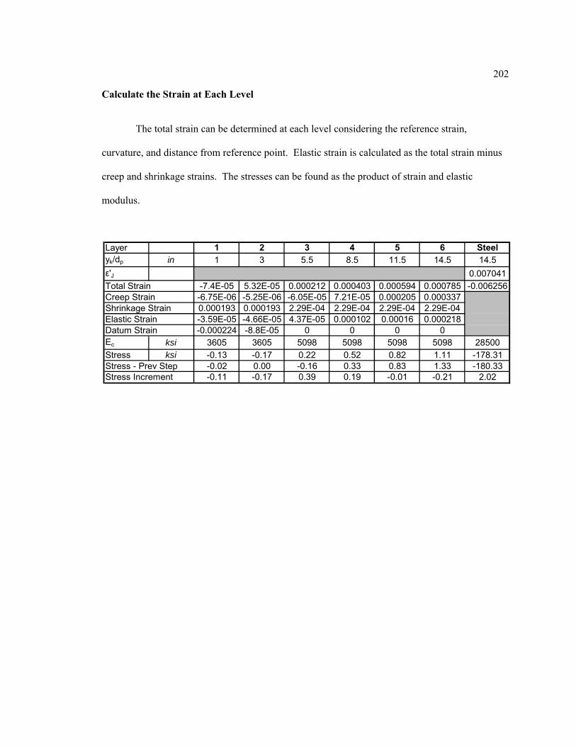
202
Calculate the Strain at Each Level
The total strain can be determined at each level considering the reference strain,
curvature, and distance from reference point. Elastic strain is calculated as the total strain minus
creep and shrinkage strains. The stresses can be found as the product of strain and elastic
modulus.
Layer 1 2 3 4 5 6 Steelyk/dp in 1 3 5.5 8.5 11.5 14.5 14.5
ε'J 0.007041
Total Strain -7.4E-05 5.32E-05 0.000212 0.000403 0.000594 0.000785 -0.006256Creep Strain -6.75E-06 -5.25E-06 -6.05E-05 7.21E-05 0.000205 0.000337Shrinkage Strain 0.000193 0.000193 2.29E-04 2.29E-04 2.29E-04 2.29E-04Elastic Strain -3.59E-05 -4.66E-05 4.37E-05 0.000102 0.00016 0.000218
-0.000224 -8.8E-05 0 0 0 0Ec ksi 3605 3605 5098 5098 5098 5098 28500
Stress ksi -0.13 -0.17 0.22 0.52 0.82 1.11 -178.31Stress - Prev Step -0.02 0.00 -0.16 0.33 0.83 1.33 -180.33Stress Increment -0.11 -0.17 0.39 0.19 -0.01 -0.21 2.02
Datum Strain

203
Time Step 7 (100 Days) [Application of SIDL]
Calculate Creep Strain at Each Level
Calculate Shrinkage Strain at Each Level
The shrinkage strain is uniform for all layers of the girder. On day 100, for concrete
steam-cured the first day, the shrinkage strain can be given as .00029. The total inelastic strain is
the sum of creep and shrinkage strain. Uniform shrinkage is also assumed for the deck concrete,
with a strain of .000378 after 20 days of drying.
Constant “A”
The constant A can be determined as follows
kipsinksiinksiinksiA 728849306.028500643605965098 222
Ec f'c Ec f'c 1 2 3 4 5 6
ksi ksi ksi ksi ksi ksi ksi ksi ksi ksi1 1 4415 6 1.124 0 0 0 0.00 0.00 -0.33 0.30 0.93 1.562 10 4769 7 0.754 0 0 0 0.00 0.00 0.01 -0.01 -0.03 -0.053 29 5098 8 0.573 0 0 0 0.00 0.00 0.12 0.03 -0.07 -0.164 30 5098 8 0.569 3224 3.2 1.46 -0.02 0.00 0.03 0.01 0.00 -0.025 31 5098 8 0.564 3420 3.6 1.238 -0.02 -0.03 0.06 0.03 0.00 -0.036 50 5098 8 0.479 3605 4 0.773 -0.10 -0.14 0.33 0.16 -0.01 -0.19
-7.1E-05 -8.8E-05 6.22E-06 0.000208 0.00041 0.000612
-0.13 -0.17 0.22 0.52 0.82 1.115098 ksi
3605 ksi
-3.6E-05 -4.7E-05 4.37E-05 0.000102 0.00016 0.000218
-3.5E-05 -4.1E-05 -3.7E-05 0.000106 0.00025 0.000394
Elastic Strain
Stress Change in Layer
φ(ti,tj)
Girder Deck
φ(ti,tj)
Previous Step Ecd
Creep Strain
Previous Step Ec
Step Day
Total Stress-Related Strain
Elastic Stress in Previous Step

204
Constants “B” and “C”
Constants “NI” and “MI”
Constants “Nd” and “Md”
1 2 3 4 5 6 SteelEc ksi 3605 3605 5098 5098 5098 5098 28500
Ak/Ap in 232 32 24 24 24 24 0.306
yk/dp in 1 3 5.5 8.5 11.5 14.5 14.5Σ
E*A*y k-in 115360 346080 672936 1039992 1407048 1774104 126454.5 B 5481975E*A*y2
k-in 115360 1038240 3701148 8839932 16181052 25724508 1833590 C 57433830
Layer
1 2 3 4 5 6 SteelEc ksi 3605 3605 5098 5098 5098 5098
Ak/Ap in 232 32 24 24 24 24
yk/dp in 1 3 5.5 8.5 11.5 14.5-3.47E-05 -4.1E-05 -3.74E-05 0.000106 0.00025 0.0003940.000378 0.000378 2.90E-04 2.90E-04 2.90E-04 2.90E-040.000343 0.000337 0.000253 0.000396 0.00054 0.000684
Σ
E*A*ε 39.59993 38.87576 30.90211 48.5096 66.11709 83.72458 NI 307.73
E*A*y*ε k-in 239.59993 116.6273 169.9616 412.3316 760.3465 1214.006 MI 2712.87
Inelastic Strain
Layer
Shrinkage StrainCreep Strain
1 2
Ec ksi 3605 3605 εod -0.000293Ak in 2
32 32 ψd -6.82E-05
yk in 1 3
Datum Strain, εd -0.000224 -8.8E-05
E*A*ε kips -25.88804 -10.15 Nd -36.04
E*A*y*ε k-in -25.88804 -30.45 Md -56.34
Layer

205
Constants “Np” and “Mp”
The relaxation stress loss from day 50 to day 100 when the prestressing steel stress is
178.3 ksi is 0.25 ksi. In addition to the 1.83 ksi from the previous step, this is an effective strain
of
000073.28500
08.2
ksi
ksi
Now an effective jacking strain will be used that is the original jacking strain minus the
effective relaxation strain
007032.000064.007105.' J
The constants can be calculated as
kipsinksiNP 33.61007032.306.28500 2
inkininksiM P 2.889007047.5.14306.28500 2
Matrix Solution
The simultaneous equations are solved by matrix methods to yield the reference strain
and curvature:
A -B εo(ti)
B -C ψ(ti)
728849 -54819755481975 -57433830
εo(ti) 1.27E-05ψ(ti) -5.91E-05
3461.73
=NI + NP + Nd
MI+MP+Md+Mapplied
333.02

206
Calculate the Strain at Each Level
The total strain can be determined at each level considering the reference strain,
curvature, and distance from reference point. Elastic strain is calculated as the total strain minus
creep and shrinkage strains. The stresses can be found as the product of strain and elastic
modulus.
Layer 1 2 3 4 5 6 Steelyk/dp in 1 3 5.5 8.5 11.5 14.5 14.5
ε'J 0.007032
Total Strain 7.17E-05 0.00019 0.000338 0.000515 0.000692 0.000869 -0.006163Creep Strain -3.47E-05 -4.1E-05 -3.74E-05 0.000106 0.00025 0.000394Shrinkage Strain 0.000378 0.000378 2.90E-04 2.90E-04 2.90E-04 2.90E-04Elastic Strain -4.71E-05 -5.92E-05 8.5E-05 0.000118 0.000152 0.000185
-0.000224 -8.8E-05 0 0 0 0Ec ksi 3605 3605 5098 5098 5098 5098 28500
Stress ksi -0.17 -0.21 0.43 0.60 0.77 0.94 -175.64Stress - Prev Step -0.13 -0.17 0.22 0.52 0.82 1.11 -178.31Stress Increment -0.04 -0.05 0.21 0.08 -0.04 -0.17 2.67
Datum Strain

207
Time Step 8 (1000 Days)
Calculate Creep Strain at Each Level
Calculate Shrinkage Strain at Each Level
The shrinkage strain is uniform for all layers of the girder. On day 1000, for concrete
steam-cured the first day, the shrinkage strain can be given as .000384. The total inelastic strain
is the sum of creep and shrinkage strain. Uniform shrinkage is also assumed for the deck
concrete, with a strain of .000605 after 70 days of drying.
Constant “A”
The constant A can be determined as follows
kipsinksiinksiinksiA 728849306.028500643605965098 222
Ec f'c Ec f'c 1 2 3 4 5 6
ksi ksi ksi ksi ksi ksi ksi ksi ksi ksi1 1 4415 6 1.489 0 0 0 0.00 0.00 -0.33 0.30 0.93 1.562 10 4769 7 0.997 0 0 0 0.00 0.00 0.01 -0.01 -0.03 -0.053 29 5098 8 0.784 0 0 0 0.00 0.00 0.12 0.03 -0.07 -0.164 30 5098 8 0.781 3224 3.2 2.349 -0.02 0.00 0.03 0.01 0.00 -0.025 31 5098 8 0.778 3420 3.6 1.979 -0.02 -0.03 0.06 0.03 0.00 -0.036 50 5098 8 0.735 3605 4 1.388 -0.10 -0.14 0.33 0.16 -0.01 -0.197 100 5098 8 0.676 3605 4 1.195 -0.04 -0.05 0.21 0.08 -0.04 -0.17
-0.00012 -0.00015 7.41E-05 0.000271 0.000468 0.000665
-0.17 -0.21 0.43 0.60 0.77 0.945098 ksi
3605 ksi
-4.7E-05 -5.9E-05 8.5E-05 0.000118 0.000152 0.000185
-7.3E-05 -8.6E-05 -1.1E-05 0.000153 0.000316 0.00048Creep Strain
Previous Step Ec
Step Day
Total Stress-Related Strain
Elastic Stress in Previous Step
Elastic Strain
Stress Change in Layer
φ(ti,tj)
Girder Deck
φ(ti,tj)
Previous Step Ecd

208
Constants “B” and “C”
Constants “NI” and “MI”
Constants “Nd” and “Md”
1 2 3 4 5 6 SteelEc ksi 3605 3605 5098 5098 5098 5098 28500
Ak/Ap in 232 32 24 24 24 24 0.306
yk/dp in 1 3 5.5 8.5 11.5 14.5 14.5Σ
E*A*y k-in 115360 346080 672936 1039992 1407048 1774104 126454.5 B 5481975E*A*y2
k-in 115360 1038240 3701148 8839932 16181052 25724508 1833590 C 57433830
Layer
1 2 3 4 5 6 SteelEc ksi 3605 3605 5098 5098 5098 5098
Ak/Ap in 232 32 24 24 24 24
yk/dp in 1 3 5.5 8.5 11.5 14.5-7.27E-05 -8.62E-05 -1.09E-05 0.000153 0.000316 0.000480.000605 0.000605 3.84E-04 3.84E-04 3.84E-04 3.84E-040.000532 0.000519 0.000373 0.000537 0.0007 0.000864
Σ
E*A*ε 61.405 59.85185 45.65197 65.67004 85.6881 105.7062 NI 423.97
E*A*y*ε k-in 261.405 179.5556 251.0858 558.1953 985.4132 1532.739 MI 3568.39
Layer
Shrinkage StrainCreep Strain
Inelastic Strain
1 2
Ec ksi 3605 3605 εod -0.000293Ak in 2
32 32 ψd -6.82E-05
yk in 1 3
Datum Strain, εd -0.000224 -8.8E-05
E*A*ε kips -25.88804 -10.15 Nd -36.04
E*A*y*ε k-in -25.88804 -30.45 Md -56.34
Layer

209
Constants “Np” and “Mp”
The relaxation stress loss from day 100 to day 1000 when the prestressing steel stress is
175.6 ksi is 0.76 ksi. In addition to the 2.08 ksi from the previous step, this is an effective strain
of
0001.28500
84.2
ksi
ksi
Now an effective jacking strain will be used that is the original jacking strain minus the
effective relaxation strain
007005.0001.007105.' J
The constants can be calculated as
kipsinksiNP 09.61007005.306.28500 2
inkininksiM P 8.885007005.5.14306.28500 2
Matrix Solution
The simultaneous equations are solved by matrix methods to yield the reference strain
and curvature:
A -B εo(ti)
B -C ψ(ti)
728849 -54819755481975 -57433830
εo(ti) 0.000181ψ(ti) -5.78E-05
4313.85
=NI + NP + Nd
MI+MP+Md+Mapplied
449.02

210
Calculate the Strain at Each Level
The total strain can be determined at each level considering the reference strain,
curvature, and distance from reference point. Elastic strain is calculated as the total strain minus
creep and shrinkage strains. The stresses can be found as the product of strain and elastic
modulus.
Interpreting the Results
The prestress loss components can be gleaned from the results by tracking the strain
changes in layer 6 (the center of gravity of the prestressing steel is in the center of layer 6). The
change in strain can be multiplied by the steel elastic modulus (Ep = 28500 ksi) to calculate the
change in prestress.
Layer 1 2 3 4 5 6 Steelyk/dp in 1 3 5.5 8.5 11.5 14.5 14.5
ε'J 0.007005
Total Strain 0.000239 0.000355 0.000499 0.000673 0.000846 0.001019 -0.005986Creep Strain -7.27E-05 -8.62E-05 -1.09E-05 0.000153 0.000316 0.00048Shrinkage Strain 0.000605 0.000605 3.84E-04 3.84E-04 3.84E-04 3.84E-04Elastic Strain -6.88E-05 -7.61E-05 0.000126 0.000136 0.000146 0.000156
-0.000224 -8.8E-05 0 0 0 0Ec ksi 3605 3605 5098 5098 5098 5098 28500Stress ksi -0.25 -0.27 0.64 0.69 0.74 0.79 -170.59
Datum Strain
Relaxation Total LossStress Stress Stress Stress Stress
ksi ksi ksi ksi ksi1 1 0 0.00 0 0.00 0.000353 10.06 0.00 10.062 10 0.000107 3.04 8.47E-05 2.41 0.000316 9.01 1.16 15.623 29 0.000257 7.32 0.000175 4.99 0.000265 7.54 1.63 21.484 30 0.000281 8.02 0.000178 5.07 0.00026 7.42 1.64 22.155 31 0.000285 8.12 0.000181 5.16 0.000254 7.25 1.65 22.186 50 0.000337 9.61 0.000229 6.53 0.000218 6.22 1.83 24.197 100 0.000394 11.24 0.00029 8.27 0.000185 5.27 2.08 26.858 1000 0.00048 13.68 0.000384 10.94 0.000156 4.43 2.84 31.90
DaysStepCreep Shrinkage Elastic
StrainStrainStrain
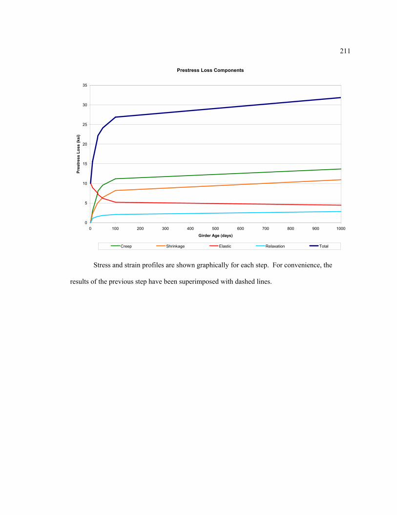
211
Stress and strain profiles are shown graphically for each step. For convenience, the
results of the previous step have been superimposed with dashed lines.
Prestress Loss Components
0
5
10
15
20
25
30
35
0 100 200 300 400 500 600 700 800 900 1000
Girder Age (days)
Pre
stre
ss L
oss
(ks
i)
Creep Shrinkage Elastic Relaxation Total

212
Strain (Step 1)
0
2
4
6
8
10
12
14
16
-0.0002 0 0.0002 0.0004 0.0006 0.0008 0.001 0.0012
Strain (Positive Indicates Shortening)
Lo
cati
on
in C
ross
-Sec
tio
n (
in)
Creep Strain Inelastic Strain Total Strain
Stress (Step 1)
0
2
4
6
8
10
12
14
16
-0.8 -0.4 0.0 0.4 0.8 1.2 1.6 2.0
Stress (ksi; + compression)
Lo
cati
on
in
cro
ss-s
ecti
on
(i
n)

213
Strain (Step 2)
0
2
4
6
8
10
12
14
16
-0.0002 0 0.0002 0.0004 0.0006 0.0008 0.001 0.0012
Strain (Positive Indicates Shortening)
Lo
cati
on
in C
ross
-Sec
tio
n (
in)
Creep Strain Inelastic Strain Total Strain
Creep Strain (Previous Step) Inelastic Strain (Previous Step) Total Strain (Previous Step)
Stress (Step 2)
0
2
4
6
8
10
12
14
16
-0.8 -0.4 0.0 0.4 0.8 1.2 1.6 2.0
Stress (ksi; + compression)
Lo
cati
on
in
cro
ss-s
ecti
on
(i
n)

214
Strain (Step 3)
0
2
4
6
8
10
12
14
16
-0.0002 0 0.0002 0.0004 0.0006 0.0008 0.001 0.0012
Strain (Positive Indicates Shortening)
Lo
cati
on
in C
ross
-Sec
tio
n (
in)
Creep Strain Inelastic Strain Total Strain
Creep Strain (Previous Step) Inelastic Strain (Previous Step) Total Strain (Previous Step)
Stress (Step 3)
0
2
4
6
8
10
12
14
16
-0.8 -0.4 0.0 0.4 0.8 1.2 1.6 2.0
Stress (ksi; + compression)
Lo
cati
on
in
cro
ss-s
ecti
on
(i
n)

215
Strain (Step 4)
0
2
4
6
8
10
12
14
16
-0.0002 0 0.0002 0.0004 0.0006 0.0008 0.001 0.0012
Strain (Positive Indicates Shortening)
Lo
cati
on
in C
ross
-Sec
tio
n (
in)
Creep Strain Inelastic Strain Total Strain
Creep Strain (Previous Step) Inelastic Strain (Previous Step) Total Strain (Previous Step)
Stress (Step 4)
0
2
4
6
8
10
12
14
16
-0.8 -0.4 0.0 0.4 0.8 1.2 1.6 2.0
Stress (ksi; + compression)
Lo
cati
on
in
cro
ss-s
ecti
on
(i
n)

216
Stress (Step 5)
0
2
4
6
8
10
12
14
16
-0.8 -0.4 0.0 0.4 0.8 1.2 1.6 2.0
Stress (ksi; + compression)
Lo
cati
on
in
cro
ss-s
ecti
on
(i
n)
Strain (Step 5)
0
2
4
6
8
10
12
14
16
-0.0002 0 0.0002 0.0004 0.0006 0.0008 0.001 0.0012
Strain (Positive Indicates Shortening)
Lo
cati
on
in
Cro
ss-S
ecti
on
(in
)
Creep Strain Inelastic Strain Total Strain
Creep Strain (Previous Step) Inelastic Strain (Previous Step) Total Strain (Previous Step)

217
Stress (Step 6)
0
2
4
6
8
10
12
14
16
-0.8 -0.4 0.0 0.4 0.8 1.2 1.6 2.0
Stress (ksi; + compression)
Lo
cati
on
in
cro
ss-s
ecti
on
(i
n)
Strain (Step 6)
0
2
4
6
8
10
12
14
16
-0.0002 0 0.0002 0.0004 0.0006 0.0008 0.001 0.0012
Strain (Positive Indicates Shortening)
Lo
cati
on
in
Cro
ss-S
ecti
on
(in
)
Creep Strain Inelastic Strain Total Strain
Creep Strain (Previous Step) Inelastic Strain (Previous Step) Total Strain (Previous Step)

218
Stress (Step 7)
0
2
4
6
8
10
12
14
16
-0.8 -0.4 0.0 0.4 0.8 1.2 1.6 2.0
Stress (ksi; + compression)
Lo
cati
on
in
cro
ss-s
ecti
on
(i
n)
Strain (Step 7)
0
2
4
6
8
10
12
14
16
-0.0002 0 0.0002 0.0004 0.0006 0.0008 0.001 0.0012
Strain (Positive Indicates Shortening)
Lo
cati
on
in
Cro
ss-S
ecti
on
(in
)
Creep Strain Inelastic Strain Total Strain
Creep Strain (Previous Step) Inelastic Strain (Previous Step) Total Strain (Previous Step)

219
8
0 0 00 0 00 0 00 0 00 0 00 0 00 0 00 0 0
Stress (Step 8)
0
2
4
6
8
10
12
14
16
-0.8 -0.4 0.0 0.4 0.8 1.2 1.6 2.0
Stress (ksi; + compression)
Lo
cati
on
in
cro
ss-s
ecti
on
(i
n)
Strain (Step 8)
0
2
4
6
8
10
12
14
16
-0.0002 0 0.0002 0.0004 0.0006 0.0008 0.001 0.0012
Strain (Positive Indicates Shortening)
Lo
cati
on
in
Cro
ss-S
ecti
on
(in
)
Creep Strain Inelastic Strain Total Strain
Creep Strain (Previous Step) Inelastic Strain (Previous Step) Total Strain (Previous Step)

220
Vita
Brian D. Swartz
Education
The Pennsylvania State University, Ph. D. Civil Engineering May 2010
Dissertation: “Time-Dependent Analysis of Pretensioned Concrete Bridge Girders”
The Pennsylvania State University, M.S. Civil Engineering August 2007
Thesis: “Development of a Design Guide for Post-Tensioned Bridge Decks”
The Pennsylvania State University, B.S. Civil Engineering May 2005
Teaching Experience
Visiting Assistant Professor, Bucknell University, Civil Engineering 2009-2010
Instructor, The Pennsylvania State University, Civil Engineering 2008-2009
Instructor, The Pennsylvania State University, SEDTAPP 2007-2008
Industry Experience
Bridge Designer, Buckland and Taylor Ltd., North Vancouver, BC June-Aug 2007
Asst. Main Span Erection Mgr. Bilfinger Berger Civil Inc., Toledo, OH May-July 2006
Bridge Design Intern, FIGG Bridge Engineers, Exton, PA May-Aug 2005
Structural Engineering Intern, Dewberry, Fairfax, VA May-Aug 2004
Bridge Inspection Intern, Pennsylvania DOT, Montoursville, PA May-Aug 2003
Professional Affiliations
American Concrete Institute
Post-Tensioning Institute, Education Committee
Publications
Swartz, B. D. and Schokker, A. J., “Development of a Design Guide for Post-Tensioned Bridge Decks,” PTI (Post-Tensioning Institute) Journal, Vol. 6 No. 2, Aug 2008