Time and memory requirements of theNonequispaced FFT

Stefan Kunis∗ Daniel Potts†

We consider the fast Fourier transform at nonequispaced nodes (NFFT)and give detailed information on the time and memory requirements of itsbuilding blocks. This manuscript reviews the state of the art approachesand focuses within the most successful scheme on the computational mostinvolved part. Beside a rigorous derivation of an lookup table technique, wecompare a wide range of precomputation schemes which lead to substantiallydifferent computation times of the NFFT. In particular, we show how tobalance accuracy, memory usage, and computation time.

Key words and phrases : Nonequispaced Fast Fourier Transform, FFT

2000 AMS Mathematics Subject Classification —

1 Introduction

This paper summarises algorithms for the discrete and fast Fourier transform at noneq-uispaced nodes. Generalising the famous fast Fourier transform (FFT), we evaluate forN ∈ 2N, M ∈ N, a vector of coefficients f = (fk)k=−N

2,..., N

2−1 ∈ CN , and a set of nodes

xj ∈ R the sums

fj =

N2−1∑

k=−N2

fke−2πikxj , j = 0, . . . , M − 1.

In the multivariate setting, the discrete Fourier transform at nonequispaced nodes (NDFT)requires O(NπM) operations for Nπ equispaced frequencies and M nonequispaced sam-pling nodes xj ∈ Rd. In contrast, the approximate NFFT takes only O(Nπ log Nπ + M)floating point operations (flops), where the constant of proportionality depends in theorysolely on the prescribed target accuracy and on the space dimension d.∗kunis@math.uni-luebeck.de, University of Lubeck, Institute of Mathematics, 23560 Lubeck, Germany†potts@mathematik.tu-chemnitz.de, Chemnitz Universitiy of Technology, Department of Mathematics,

09107 Chemnitz, Germany

1

There is a variety of important applications which utilise the NDFT, e.g. in com-puterised tomography, for fast summation algorithms [25], as fast Fourier transform onthe sphere [19], or as part of the ridgelet and curvelet transforms [11, 5]. Furthermore,the reconstruction from nonuniform samples is stated in [10, 1, 20] as inversion of theNDFT and used for example in magnetic resonance imaging [12]. In each of these ap-plications, the actual computation of the NDFT is the computationally dominant taskand one has to deal with different requirements on the NFFT with respect to the tar-get accuracy, the usage of memory, and the actual computation time. An early reviewof several algorithms for the NFFT is given in [29]. Only later, a unified approach tofast algorithms for the present task was obtained in [27, 26] and recently, a particularproperty of the Gaussian window function was utilised in [15] to speed up computationswhen no precomputation is possible.

Despite the fact, that there exist a couple of tutorial papers for the NFFT (see also[16]), the aim of this manuscript is to give detailed information on the accuracy, memory,and time requirements of NFFT algorithms and to describe how to balance these factors.In particular, the O(M)-step of the NFFT hides a significant constant and we focus ona variety of precomputation schemes which lead to substantially different computationtimes of the whole NFFT.

The outline of the paper is as follows. In Section 2 minor improvements in the directcalculation of the NDFT are discussed, cf. [2]. Furthermore the unified approach tothe NFFT is reviewed and alternative NFFTs are discussed. In Section 3 we comparedifferent methods for the fast evaluation and precomputation of the most popular windowfunctions. Finally, we compare the different NFFTs numerically in Section 4 and drawconclusions. All used algorithms are available as pre-release of an upcoming version ofour widely used software [18].

2 Notation, the NDFT and the NFFT

This section summarises the mathematical theory and ideas behind the NFFT. Ford, M ∈ N let the torus Td := Rd/Zd ∼ [−1

2 , 12)d and the sampling set X := {xj ∈ Td :

j = 0, . . . , M−1} be given. Furthermore, let the multi degree N = (N0, N1, . . . , Nd−1)> ∈

2Nd and the index set for possible frequencies IN := {−N02 , N0

2 −1}×. . .×{−Nd−1

2 ,Nd−1

2 −1} be given. We define the space of d-variate trigonometric polynomials TN of multidegree N by

TN := span{

e−2πik· : k ∈ IN

}

The dimension of this space and hence the total number of Fourier coefficients is Nπ =N0 · . . . ·Nd−1. Note, that we abbreviate the inner product between the frequency k andthe time/spatial node x by kx = k>x = k0x0 + k1x1 + . . . + kd−1xd−1. For clarity ofpresentation the multi index k addresses elements of vectors and matrices as well.

2

2.1 NDFT

For a finite number of given Fourier coefficients fk ∈ C, k ∈ IN , one wants to evaluatethe trigonometric polynomial

f (x) :=∑

k∈IN

fke−2πikx (2.1)

at given nonequispaced nodes xj ∈ Td, j = 0, . . . , M − 1. Thus, our concern is thecomputation of the matrix vector product

f = Af (2.2)

where

f := (f (xj))j=0,...,M−1 , A :=(e−2πikxj

)j=0,...,M−1; k∈IN

, f :=(fk

)k∈IN

.

The straight forward algorithm for this matrix vector product, which is called NDFTin Algorithm 1, takes O(MNπ) arithmetical operations and stores no matrix elementsat all, but rather uses MNπ direct calls of the function cexp() to evaluate the complexexponentials e−2πikxj .

Input: d, M ∈ N, N ∈ 2Nd,xj ∈ [−1

2 , 12 ]d, j = 0, . . . , M − 1, and fk ∈ C, k ∈ IN .

for j = 0, . . . , M − 1 dofj = 0for k ∈ IN do

fj+ = fke−2πikxj

end forend for

Output: values fj = f(xj), j = 0, . . . , M − 1.

Algorithm 1: NDFT

Related matrix vector products are the adjoint NDFT

f = Aaf , fk =M−1∑

j=0

fje2πikxj ,

where the update step in Algorithm 1 is simply changed to fk+ = fje2πikxj , the con-jugated NDFT f = Af , and the transposed NDFT f = A>f where Aa = A

>. Notefurthermore, that the inversion formula F−1 = F a for the (equispaced and normalised)Fourier matrix F does not hold in the general situation of arbitrary sampling nodes forthe matrix A.

3

NDFT acceleration

Algorithm 1 evaluates MNπ complex exponentials. Due to the fact that these directcalls are more expensive than multiplications, we may basically change the update stepto fj = fje2πixj + fk (d = 1), i.e., do a Horner-like-scheme, see also [2]. Hence, in general2dM direct calls are sufficient for the computations in Algorithm 1. Note however, thatthis approach looses numerical stability to some extend, cf. [28]. Trading even morememory for the acceleration of the computation, one might precompute all entries of thematrix A, which is only feasible for small Nπ and M , see Example 4.1 in Section 4.

NDFT method memory flops evaluationsstandard - MNπ MNπ

Horner-like - MNπ 2dMfully precomputed MNπ MNπ -

Table 2.1: Number of precomputed and stored complex exponentials (memory), the or-der of magnitude for the number of floating point operations (flops), and thenumber of evaluations for the function cexp() (evaluations).

2.2 NFFT

The most successful approach for the fast computation of (2.2), cf. [7, 4, 27, 26, 13, 12,15], is based on the usage of an oversampled FFT and a window function ϕ which issimultaneously localised in time/space and frequency. Basically, the scheme utilises theconvolution theorem in the following three informal steps:

1. deconvolve the trigonometric polynomial f in (2.1) with the window function infrequency domain,

2. compute an oversampled FFT on the result of step 1., and

3. convolve the result of step 2. with the window function in time/spatial domain;evaluate this convolution at the nodes xj .

Throughout the rest of the paper σ > 1 and n = σN ∈ N will denote the oversamplingfactor and the FFT size, respectively. Furthermore, for d > 1 let σ ∈ Rd, σ0, . . . , σd−1 >1, n = σ ¯ N , and nπ = n0 · . . . · nd−1 denote the oversampling factor, the FFTsize, and the total FFT size, respectively. Here, we use for notational convenience thepointwise product σ ¯ N := (σ0N0, σ1N1, . . . , σd−1Nd−1, )

> with its inverse N−1 :=(1

N0, 1

N1, . . . , 1

Nd−1

)>.

The window function

Starting with a window function ϕ ∈ L2(R), which is well localised in the time/spatialdomain R and in the frequency domain R, respectively, one assumes that its 1-periodic

4

version ϕ, i.e.,ϕ (x) :=

∑

r∈Zϕ (x + r)

has an uniformly convergent Fourier series and is well localised in the time/spatial do-main T and in the frequency domain Z, respectively. Thus, the periodic window functionϕ may be represented by its Fourier series

ϕ (x) =∑

k∈Zϕ (k) e−2πikx

with the Fourier coefficients

ϕ (k) :=∫

T

ϕ (x) e2πikx dx =∫

R

ϕ (x) e2πikx dx , k ∈ Z.

We truncate this series at the FFT length n which causes a aliasing error.If ϕ is furthermore well localised in time/spatial domain R, it can be truncated with

truncation parameter m ∈ N, m ¿ n and approximated by the function ϕ·χ[−mn

, mn

] whichhas compact support within the interval [−m

n , mn ]. Furthermore, the periodic window

function can be approximated by the periodic version of the truncated window function.For d > 1, univariate window functions ϕ0, . . . , ϕd−1, and a node x = (x0, . . . , xd−1)>

−0.5 −0.1 0 0.1 0.5

10−15

10−10

10−5

100

−60 −45 −15 0 14 44 60

10−15

10−10

10−5

100

Figure 2.1: Left: Gaussian window function ϕ(x) = c e−αx2(solid), cf. (3.1), and its

1-periodic version ϕ sampled on 2m + 1 nodes x0− mn , x0− m−1

n , . . . , x0 + mn

denoted by ¦ where x0 = 0; Right: integral Fourier transform ϕ with pass(¦), transition, and stop band (×); for the parameters N = 30, σ = 2, n =60, m = 6.

the multivariate window function is simply given by

ϕ (x) := ϕ0 (x0) ϕ1 (x1) . . . ϕd−1 (xd−1) , (2.3)

5

where ϕ(x) =∑

r∈Zd ϕ(x + r) again denotes the 1-periodic version; an immediate ob-servation is

ϕ (k) :=∫

Rd

ϕ (x) e2πikx dx = ϕ0 (k0) ϕ1 (k1) . . . ϕd−1 (kd−1) .

For a single truncation parameter m ∈ N the window function is truncated to the cuben−1 ¯ [−m, m]d.

We follow the general approach of [27, 26] and approximate the complex exponentialsin the trigonometric polynomial (2.1) by

e−2πikx ≈ 1nπϕ (k)

∑

l∈In,m(x)

ϕ(x− n−1 ¯ l

)e−2πi(n−1¯l)k (2.4)

where the set

In,m (x) := {l ∈ In : n¯ x−m1 ≤ l ≤ n¯ x + m1}

collects these indices where the window function is mostly concentrated (the inequalitieshave to be fulfilled modulo n and for each component). After changing the order ofsummation in (2.1) we obtain for xj ∈ Td, j = 0, . . . ,M − 1, the approximation

f (xj) ≈∑

l∈In,m(xj)

∑

k∈IN

fk

nπϕ (k)e−2πi(n−1¯l)k

ϕ

(xj − n−1 ¯ l

).

This causes a truncation and an aliasing error, see [26, 24] for details. As can be readilyseen, after an initial deconvolution step, the expression in brackets can be computedvia a d-variate FFT of total size nπ. The final step consists of the evaluation of sumshaving at most (2m + 1)d summands where the window function is sampled only in theneighbourhood of the node xj .

The algorithm and its matrix notation

The proposed scheme reads in matrix vector notation as

Af ≈ BFDf , (2.5)

where B denotes the real M × nπ sparse matrix

B :=(ϕ

(xj − n−1 ¯ l

) · χIn,m(xj) (l))

j=0,...,M−1; l∈In

, (2.6)

where F is the d-variate Fourier matrix of size nπ×nπ, and where D is the real nπ×Nπ

’diagonal’ matrix

D :=d−1⊗

t=0

(Ot | diag (1/ ϕt (kt))kt∈INt

|Ot

)>

6

Method memory flops evaluations- - Nπ Nπ

PRE PHI HUT N0 + . . . + Nd−1 Nπ -

Table 2.2: Computational requirements for the deconvolution step in Algorithm 2.

with zero matrices Ot of size Nt × nt−Nt2 . Obviously, the approximate matrix splitting

can by applied to the adjoint matrix as Aa ≈ D>F aB>, where the multiplication withthe sparse matrix B> is implemented in a ’transposed’ way, summation as outer loopand only using the index sets In,m (xj).

Table 2.2 shows the computational requirements for the deconvolution step of theNFFT. We give detailed information on the number of precomputed and stored realnumbers (memory), the order of magnitude for the number of floating point operations(flops), and the number of evaluations for the univariate Fourier-transformed windowfunction ϕ. Precomputing the factors ϕt(kt) for t = 0, . . . , d− 1 and kt ∈ INt is denotedby its associated Flag PRE PHI HUT within the software library.

This is followed by one FFT of total size nπ. Hence, the computational complexity ofthe NFFT increases for a larger oversampling factor σ, affecting both the ’deconvolutionstep’ and the FFT. The time and memory requirements of the convolution and evalu-ation step are discussed in Section 3 in detail. In summary, we propose Algorithm 2and Algorithm 3 for the computation of the nonequispaced FFT (2.2) and its adjoint,respectively.

Input: d, M ∈ N, N ∈ 2Nd,xj ∈ [−1

2 , 12 ]d, j = 0, . . . , M − 1, and fk ∈ C, k ∈ IN .

For k ∈ IN compute

gk :=fk

nπck (ϕ).

For l ∈ In compute by d-variate FFT

gl :=∑

k∈IN

gk e−2πik(n−1¯l).

For j = 0, . . . , M − 1 compute

sj :=∑

l∈In,m(xj)

gl ϕ(xj − n−1 ¯ l

).

Output: approximate values sj ≈ fj , j = 0, . . . , M − 1.

Algorithm 2: NFFT

7

Input: d,M ∈ N, N ∈ 2Nd,xj ∈ [−1

2 , 12 ]d and fj ∈ C, j = 0, . . . , M − 1.

Compute the sparse matrix vector product

g := B>f .

Apply the d-variate IFFT asg := F ag .

Multiply by the ’diagonal’ matrix, i.e.,

s := D>g .

Output: approximate values sk, k ∈ IN .

Algorithm 3: NFFTa

Alternative NFFTs

Taylor based NFFT: A simple but nevertheless fast scheme for the computation of(2.2) in the univariate case d = 1 is presented in [1]. This approach uses for eachnode xj ∈ [−1

2 , 12) a m-th order Taylor expansion of the trigonometric polynomial

in (2.1) about the nearest neighbouring point on the oversampled equispaced lattice{n−1k − 1

2}k=0,...,n−1 where again n = σN, σ À 1. Besides its simple structure andonly O(N log N + M) arithmetic operations, this algorithm utilises m FFTs of size ncompared to only one in the NFFT approach, uses a medium amount of extra memory,and is not suited for highly accurate computations, see Example 4.2. Furthermore, itsextension to higher dimensions has not been considered so far.Multipole based NFFT: A second approach for the univariate case d = 1 is consideredin [8] and based on a Lagrange interpolation technique. After taking a N -point FFT ofthe vector f in (2.2) one uses an exact polynomial interpolation scheme to obtain thevalues of the trigonometric polynomial f at the nonequispaced nodes xj . Here, the timeconsuming part is the exact polynomial interpolation scheme which can however be re-alised fast in an approximate way by means of the fast multipole method. This approachis appealing since it allows also for the inverse transform. Nevertheless, numerical ex-periments in [8] showed that this approach is far more time consuming than Algorithm2 and the inversion can only be computed in a stable way for almost equispaced nodes[8].Linear algebra based NFFT: Using a fully discrete approach, one might fix theentries of the ’diagonal’ matrix D in (2.5) first and precompute optimised entries for thesparse matrix B to achieve higher accuracy, cf. [22, 23]. A similar approach, based onmin-max interpolation, has been taken within [12]. While these approaches gain someaccuracy for the Gaussian or B-Spline windows, no reasonable improvement is obtained

8

for the Kaiser-Bessel window function. Since it is more expensive to precompute theseoptimised entries of the matrix B, we do not further consider these schemes.

3 Evaluation techniques for window functions

To keep the aliasing error and the truncation error small, several univariate functions ϕwith good localisation in time and frequency domain were proposed. For an oversamplingfactor σ > 1, a degree N ∈ 2N, the FFT length n = σN , and a cut-off parameter m ∈ N,the following window functions are considered:

1. for a shape parameter b = 2σ2σ−1

mπ the dilated Gaussian window [7, 27, 6]

ϕ (x) = (πb)−1/2 e−(nx)2

b , (3.1)

2. for M2m denoting the centred cardinal B-Spline of order 2m the dilated B-Splinewindow [4, 27]

ϕ (x) = M2m (nx) , (3.2)

3. the dilated Sinc window [24]

ϕ (x) = sinc2m

((2σ − 1)N

2mπx

)(3.3)

with sinc(x) := sin(x) / x for x 6= 0 and sinc(0) := 1

4. and for a shape parameter b = π(2− 1σ ) the dilated Kaiser-Bessel window [25]

ϕ (x) =1π

sinh(b√

m2−n2x2)√m2−n2x2

for |x| ≤ mn ,

sin(b√

n2x2−m2)√n2x2−m2

otherwise.

(3.4)

Note, that the latter two have compact support in frequency domain while the secondone has compact support in time domain. Further references on the usage of (gener-alised) Kaiser-Bessel window functions include [17, 13, 21], where some authors preferto interchange the role of time and frequency domain. For these univariate windowfunctions ϕ, the error introduced by Algorithm 2 obeys

|f (xj)− sj | ≤ Cσ,m‖f‖1 (3.5)

where

Cσ,m :=

4 e−mπ(1−1/(2σ−1)) for (3.1), cf. [27],

4(

12σ−1

)2mfor (3.2), cf. [27],

1m−1

(2

σ2m +(

σ2σ−1

)2m)

for (3.3), cf. [24],

4π (√

m + m) 4

√1− 1

σ e−2πm√

1−1/σ for (3.4), cf. [24].

9

Thus, for fixed σ > 1, the approximation error introduced by the NFFT decays expo-nentially with the number m of summands in (2.4). Using the tensor product approach,the above error estimates have been generalised for the multivariate setting in [9, 6].Note furthermore, that it is convenient to replace the periodic window function ϕ againby the original one ϕ within the actual computation. This causes an error for functionswith large support in time/spatial domain. However, whenever the FFT-length n isreasonable ’large’, e.g., n ≥ max{4m, 12} for the Gaussian, an easy calculation showsthat for x ∈ [−m

n , mn ] the estimate

|ϕ (x)− ϕ (x)||ϕ (x)| =

∑

r∈Z\{0}e−

n2

br(r−2x) < 10−16

holds true, i.e., the made error is within machine precision. If the restriction on n is notfulfilled, the NDFT method is competitive, anyway.

In the following, we suggest different methods for the compressed storage and appli-cation of the matrix B which are all available within our NFFT library by choosingparticular flags in a simple way during the initialisation phase. These methods do notyield a different asymptotic performance but rather yield a lower constant in the amountof computation.

3.1 Fully precomputed window function

One possibility is to precompute all values ϕ(xj −n−1¯ l) for j = 0, . . . , M − 1 and l ∈In,m(xj) explicitly. Thus, one has to store the large amount of (2m+1)dM real numbersbut uses no extra floating point operations during the matrix vector multiplication besidethe necessary (2m + 1)dM flops. Furthermore, we store for this method explicitly therow and column for each nonzero entry of the matrix B. This method, included by theflag PRE FULL PSI, is the fastest procedure but can only be used if enough main memoryis available.

3.2 Tensor product based precomputation

Using the fact that the window functions are built as tensor products one can storeϕt((xj)t − lt

nt) for j = 0, . . . ,M − 1, t = 0, . . . , d − 1, and lt ∈ Int,m((xj)t) where (xj)t

denotes the t-th component of the j-th node. This method uses a medium amount ofmemory to store d(2m + 1)M real numbers in total. However, one has to carry outfor each node at most 2(2m + 1)d extra multiplications to compute from the factors themultivariate window function ϕ(xj−n−1¯ l) for l ∈ In,m(xj). Note, that this techniqueis available for every window function discussed here and can be used by means of theflag PRE PSI which is also the default method within our software library.

3.3 Linear interpolation from a lookup table

For a large number of nodes M , the amount of memory can by further reduced by the useof lookup table techniques. For a recent example within the framework of gridding see

10

[3]. We suggest to precompute from the even window function the equidistant samplesϕt( rm

Knt) for t = 0, . . . , d − 1 and r = 0, . . . , K, K ∈ N and then compute for the

actual node xj during the NFFT the values ϕt((xj)t − ltnt

) for t = 0, . . . , d− 1 and lt ∈Int,m((xj)t) by means of the linear interpolation from its two neighbouring precomputedsamples.

Lemma 3.1 For the univariate window functions (3.1) - (3.4) and K ∈ N the linearinterpolated window function, denoted by ϕK , fulfils

max|x|≤m

n

|ϕ (x)− ϕK (x)| ≤

(2σ − 1

σ

)3/2 π√

2m

16K2for (3.1) ,

m2

4K2for (3.2) ,

m (2σ − 1)2 π2

48σ2K2for (3.3) ,

e2πm

8K2for (3.4) .

Proof: From standard error estimates, we know that the linear interpolated windowfunction ϕK fulfils

max|x|≤m

n

|ϕ (x)− ϕK (x)| ≤ m2

8K2n2max|ξ|≤m

n

∣∣ϕ′′ (ξ)∣∣ . (3.6)

The maximum of this second derivative is met for the window functions (3.1) - (3.4) atξ = 0. Thus, the assertion follows by

|ϕ′′(0)| =

(2σ − 1

σm

)3/2 πn2

√2

for (3.1) ,

2n2 (M2m−2 (0)−M2m−2 (1)) for (3.2) ,

(2σ − 1)2 π2n2

6mσ2for (3.3) ,

n2

2m3π(bm cosh (bm)− sinh (bm)) for (3.4) ,

and the estimates M2m−2 (0)−M2m−2 (1) ≤ 1 and bm cosh(bm)− sinh(bm) ≤ 2πm e2πm.

This method needs only a storage of dK real numbers in total where K depends solelyon the target accuracy but neither on the number of nodes M nor on the multi degreeN . Choosing K to be a multiple of m, we further reduce the computational costs duringthe interpolation since the distance from (xj)t− lt

ntto the two neighbouring interpolation

nodes and hence the interpolation weights remain the same for all lt ∈ Int,m((xj)t). Thismethod requires 2(2m+1)d extra multiplications per node and is used within the NFFTby the flag PRE LIN PSI.

11

3.4 Fast Gaussian gridding

Two useful properties of the Gaussian window function (3.1) within the present frame-work were recently reviewed in [15]. Beside its tensor product structure for d > 1, whichalso holds for all other window functions, it is remarkable that the number of evaluationsof the form exp() can be greatly decreased. More precisely, for d = 1 and a fixed nodexj the evaluations of ϕ(xj − l′

n), l′ ∈ In,m(xj), can be reduced by the splitting

√πbϕ

(xj − l′

n

)= e−

(nxj−l′)2b = e−

(nxj−u)2

b

(e−

2(nxj−u)

b

)l

e−l2

b .

where u = min In,m(xj) and l = 0, . . . , 2m. Note, that the first factor and the expo-nential within the brackets are constant for each fixed node xj . Once, we evaluate thesecond exponential, its l-th power can be computed consecutively by multiplicationsonly. Furthermore, the last exponential is independent of xj and these 2m+1 values arecomputed only once within the NFFT and their amount is negligible. Thus, it is suffi-cient to store or evaluate 2M exponentials for d = 1. The case d > 1 uses 2dM storagesor evaluations by using the general tensor product structure. This method is employedby the flags FG PSI and PRE FG PSI for the evaluation or storage of 2 exponentials pernode, respectively.

3.5 No precomputation of the window function

The last considered method uses no precomputation at all, but rather evaluates theunivariate window function (2m + 1)dM times. Thus, the computational time dependson how fast we can evaluate the particular window function. However, no additionalstorage is necessary which suits this approach whenever the problem size reaches thememory limits of the used computer.

3.6 Summary on the computational costs

The multiplication with the sparse matrix B clearly takes O(mdM) operations. Besidethis, Table 3.1 summarises the memory requirements for different strategies to store theelements of this matrix and the extra costs it takes to multiply with this ’compressed’matrix.

4 Numerical experiments

We present numerical experiments in order to demonstrate the performance of our al-gorithms. All algorithms were implemented in C and tested on an AMD AthlonTMXP2700+ with 2GB main memory, SuSe-Linux (kernel 2.4.20-4GB-athlon, gcc 3.3) usingdouble precision arithmetic. Moreover, we have used the libraries FFTW 3.0.1 [14] andan extended version of NFFT 2.0.3 [18]. In order to reproduce all the numerical results,a pre-release of the upcoming NFFT library can be downloaded from our web page [18].

12

Method memory extra flops evaluations- - ∗ mdMFG PSI - dm,∗ dMPRE LIN PSI dK dm,∗ -PRE FG PSI dM dm,∗ -PRE PSI dmM ∗ -PRE FULL PSI mdM - -

Table 3.1: Theoretical order of magnitude for memory requirements, extra floating pointoperations, and the evaluations of the window function ϕ. Furthermore,at most 2(2m + 1)d multiplications are used within each scheme besidesPRE FULL PSI to compute the multivariate window function out of its uni-variate factors, denoted by ∗.

Example 4.1 We start by examining accelerated NDFTs for d = 1. Using the threeproposed possibilities to compute the matrix vector product by either MN direct calls ofcexp(), a Horner-like scheme, or a fully precomputed matrix A, we obtain the followingtimings for increasing N in Figure 4.1 (top-left). Clearly, the complete precomputationof the matrix A does not pay off. The Horner-like NDFT uses no extra memory andis considerably faster than the NDFT. Furthermore, it is faster than the default NFFTuntil an break even of N = 128.

Example 4.2 Our second example concerns the Taylor expansion based NFFT, againonly for d = 1. We note that this scheme actually provides a competitive NFFT withrespect to the computation time relative to the problem size - at least within a factor,cf. Figure 4.1 (top-right). The main drawbacks of this approach are its instability, i.e.,it is not possible to obtain high accurate results by increasing the order m of the Taylorexpansion and hence the number of used FFTs. This fact remains even true for a verylarge oversampling factor σ = 16, see Figure 4.1 (bottom-left). Furthermore, even whenthe target accuracy E∞ = ‖f − s‖∞ / ‖f‖∞, cf. [1], is somewhat larger, the NFFTneeds considerable fewer arithmetic operations to reach it, cf. 4.1 (bottom-right).

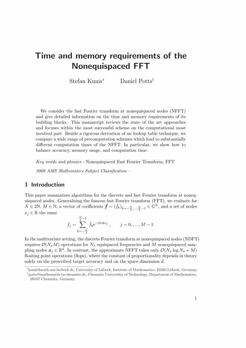
Example 4.3 We now compare the computation time for the three tasks within theNFFT, i.e., the deconvolution step, the oversampled FFT, and the convolution/evaluationstep for space dimension d = 1. Figure 4.2 shows the timings for increasing degree N ,M = N nodes, and a fixed cut-off m = 4. The linear dependence of the computation timewith respect to the problem size can be seen for the matrix-vector multiplication withthe ’diagonal’ matrix D and the sparse matrix B whereas the FFT takes O(N log N)operations.

For the deconvolution step we obtain a speed up of more than 3 by avoiding directcalls of the Fourier-transformed window function ϕ, this method is default and turnedon by the precomputation flag PRE PHI HUT, cf. Figure 4.2 (top-left). Ways to speedup the FFT by a more exhaustive search of an optimal FFT-plan are discussed in [14],

13

Figure 4.2 (top-right) shows for larger degree N a speed up of around 2 when we usethe planner FFTW MEASURE, which is also default within the NFFT.

The time to compute the last step of the NFFT differs from no precomputation ofthe matrix entries of B to explicitly precomputed entries with PRE FULL PSI by a factorof 20 to 100 for small degrees N ≤ 2048 and by a factor of 5 to 20 for larger degrees.Note however, that the use of this flag with ’maximal precomputation’ is limited by theavailable memory, e.g. for m = 4, and M = 220 we already need 144 MByte just forstoring the matrix entries and its indices.

Example 4.4 Furthermore, we show the timings of the convolution/evaluation step forincreasing N , the multi degree N = (N, . . . , N)>, M = Nd nodes, a fixed cut-off m = 4,and space dimension d = 2, 3 in Figure 4.3. Note, that for d = 2 and m = 4 the matrixB has already 81 nonzero entries per row.

Example 4.5 More detailed, we focus on the convolution/evaluation step for spacedimension d = 1. Figure 4.4 shows the computation time with respect to achievedtarget accuracy E2 = ‖f − s‖2 / ‖f‖2, cf. [26], by increasing the cut-off m for fixeddegree and number of nodes.

We conclude, that if no additional memory is used for precomputing the entries of thematrix B, the Gaussian window function in conjunction with the flag FG PSI performsbest, cf. Figure 4.4 (top-left). If no precomputation is used, the particular bad behaviourof the B-Spline window function is due to the fact that evaluating this window functiononce already takes O(m) operations.

When only a small amount of memory is used for precomputations, the decision be-tween the linear interpolated Kaiser-Bessel window function and the fast Gaussian grid-ding with precomputation PRE FG PSI depends on the accuracy one would like to achieve- here, the linear interpolated Kaiser-Bessel window performs better up to single preci-sion (top-right).

Whenever at least 2mM values can be precomputed, the Kaiser-Bessel window per-forms always best, i.e., needs the least time to achieve a given target accuracy, cf. Figure4.4 (bottom).

Example 4.6 Finally, Figure 4.5 shows the quadratic decay of the error introduced bythe linear interpolation of the window function if the method PRE LIN PSI is used. Thedecay of the error E2 coincides for all window functions up to the accuracy, they actuallycan provide for a fixed cut-off m = 10.

5 Conclusions

Fast algorithms for the nonequispaced discrete Fourier transform are already known acouple of years. Besides their asymptotic computational complexity of O(Nπ log Nπ +

14

M) for Nπ equispaced frequencies and M nonequispaced sampling nodes, NFFTs differsubstantially in their computation time for interesting problem sizes. For its actualusage, we summarise:

1. If the problem size is really small, e.g. N = M < 32 for d = 1, just use the NDFTor its Horner-like derivative.

2. The simplest fast method is the Taylor expansion based NFFT, it achieves noteven single precision, needs a somewhat larger oversampling factor, and is slowerthan window function based methods.

3. If the problem barely fits into your computer, you should use the fast Gaussiangridding NFFT, i.e., the Gaussian window function in conjunction with the flagFG PSI which uses no extra memory.

4. Using only a small amount of memory for precomputation and asking for highaccuracy, the fast Gaussian gridding NFFT with precomputation performs bestwhile storing 2d real numbers per node. However, the Kaiser-Bessel window inconjunction with the lookup table method PRE LIN PSI with 212 precomputedvalues suffices for single precision 10−8, regardless of the problem size, and out-performs the fast Gaussian gridding. Furthermore, the lookup table is the onlyprecomputation method which is independent of the actual sampling set {xj}.

5. If a medium amount of memory can be used for precomputation, the Kaiser-Besselwindow function performs best. The tensor product based precomputation schemePRE PSI yields a faster NFFT than the lookup table method or the fast Gaussiangridding with precomputation, but stores for each node dm real numbers. Forsmall to medium size problems, one can gain another factor 2 to 5 by means of anfully precomputed window function PRE FULL PSI. However, this causes a storagecost of md real numbers per sampling node.

6. Default precomputation methods, selected by the simple initialisation routine ofthe NFFT, are: PRE PHI HUT for the deconvolution step, the flag FFTW MEASURE forplanning the FFT, and the tensor product based precomputation scheme PRE PSIfor the convolution/evaluation step. Furthermore, the Kaiser-Bessel window func-tion is selected as default at compilation.

Acknowledgement

The first author is grateful for support of this work by the German Academic ExchangeService (DAAD) and the warm hospitality during his stay at the Numerical HarmonicAnalysis Group, University of Vienna. Furthermore, we would like to thank Matt Fulker-son for contributing an early version of the fast Gaussian gridding to the NFFT software.

15

References

[1] C. Anderson and M. Dahleh. Rapid computation on the discrete Fourier transform.SIAM J. Sci. Comput., 17:913 – 919, 1996.

[2] S. Bagchi and S. Mitra. The nonuniform discrete Fourier transform. In F. Marvasti,editor, Nonuniform Sampling: Theory and Practice. Kluwer/Plenum, 2001.

[3] P. Beatty, D. Nishimura, and J. Pauly. Rapid gridding reconstruction with a mini-mal oversampling ratio. IEEE Trans. Med. Imag., 24:799 – 808, 2005.

[4] G. Beylkin. On the fast Fourier transform of functions with singularities. Appl.Comput. Harmon. Anal., 2:363 – 381, 1995.

[5] E. Candes, L. Demanet, D. Donoho, and L. Ying. Fast discrete curvelet transforms.SIAM Multiscale Model. Simul., to appear.

[6] A. J. W. Duijndam and M. A. Schonewille. Nonuniform fast Fourier transform.Geophysics, 64:539 – 551, 1999.

[7] A. Dutt and V. Rokhlin. Fast fourier transforms for nonequispaced data. SIAM J.Sci. Stat. Comput., 14:1368 – 1393, 1993.

[8] A. Dutt and V. Rokhlin. Fast Fourier transforms for nonequispaced data II. Appl.Comput. Harmon. Anal., 2:85 – 100, 1995.

[9] B. Elbel and G. Steidl. Fast Fourier transform for nonequispaced data. In C. K.Chui and L. L. Schumaker, editors, Approximation Theory IX, Nashville, 1998.Vanderbilt University Press.

[10] H. Feichtinger, K. Grochenig, and T. Strohmer. Efficient numerical methods innon-uniform sampling theory. Numer. Math., 69:423 – 440, 1995.

[11] M. Fenn and J. Ma. Combined complex ridgelet shrinkage and total variationminimization. SIAM J. Sci. Comput., 2005. accepted.

[12] J. A. Fessler and B. P. Sutton. Nonuniform fast Fourier transforms using min-maxinterpolation. IEEE Trans. Signal Process., 51:560 – 574, 2003.

[13] K. Fourmont. Non equispaced fast Fourier transforms with applications to tomog-raphy. J. Fourier Anal. Appl., 9:431 – 450, 2003.

[14] M. Frigo and S. G. Johnson. FFTW, a C subroutine library. http://www.fftw.org/.

[15] L. Greengard and J.-Y. Lee. Accelerating the nonuniform fast Fourier transform.SIAM Rev., 46:443 – 454, 2004.

[16] J. A. Hogan and J. D. Lakey. Time-Frequency and Time-Scale Methods: Wavelets,Sampling, Uncertainty Principles. Applied and Numerical Harmonic Analysis series.Birkhauser, Boston, 2005.

16

[17] J. I. Jackson. Selection of a convolution function for Fourier inversion using gridding.IEEE Trans. Med. Imag., 10:473 – 478, 1991.

[18] S. Kunis and D. Potts. NFFT, Softwarepackage, C subroutine library.http://www.math.uni-luebeck.de/potts/nfft, 2002 – 2005.

[19] S. Kunis and D. Potts. Fast spherical Fourier algorithms. J. Comput. Appl. Math.,161:75 – 98, 2003.

[20] S. Kunis and D. Potts. Stability results for scattered data interpolation by trigono-metric polynomials. Preprint, Univ. Lubeck, A-04-12, 2004.

[21] S. Matej, J. Fessler, and I. Kazantsev. Iterative tomographic image reconstructionusing Fourier-based forward and back- projectors. IEEE Trans. Med. Imag., 23:401– 412, 2004.

[22] N. Nguyen and Q. H. Liu. The regular Fourier matrices and nonuniform fast Fouriertransforms. SIAM J. Sci. Comput., 21:283 – 293, 1999.

[23] A. Nieslony and G. Steidl. Approximate factorizations of Fourier matrices withnonequispaced knots. Linear Algebra Appl., 266:337 – 351, 2003.

[24] D. Potts. Schnelle Fourier-Transformationen fur nichtaquidistante Daten und An-wendungen. Habilitation, Universitat zu Lubeck, 2003.

[25] D. Potts and G. Steidl. Fast summation at nonequispaced knots by NFFTs. SIAMJ. Sci. Comput., 24:2013 – 2037, 2003.

[26] D. Potts, G. Steidl, and M. Tasche. Fast Fourier transforms for nonequispaced data:A tutorial. In J. J. Benedetto and P. J. S. G. Ferreira, editors, Modern SamplingTheory: Mathematics and Applications, pages 247 – 270, Boston, 2001. Birkhauser.

[27] G. Steidl. A note on fast Fourier transforms for nonequispaced grids. Adv. Comput.Math., 9:337 – 353, 1998.

[28] M. Tasche and H. Zeuner. Roundoff error analysis for fast trigonometric transforms.In Handbook of Analytic-Computational Methods in Applied Mathematics, pages 357– 406, CRC Press, Boca Raton, 2000.

[29] A. F. Ware. Fast approximate Fourier transforms for irregularly spaced data. SIAMRev., 40:838 – 856, 1998.

17

102

103

104

105

10−6

10−4

10−2

100

102

102

103

104

105

106

10−6

10−4

10−2

100

102

5 10 15 2010

−15

10−10

10−5

100

10−10

10−5

10−2

10−1

Figure 4.1: Comparison of different NDFTs and the Taylor expansion based NFFT withthe (window function based) NFFT for the univariate case d = 1. Top: Com-putation time in seconds with respect to increasing degree N = 24, . . . , 222

and M = N . Left: NDFT (solid), Horner-like NDFT (dashed), Multiplica-tion with fully precomputed Matrix A (dash-dot), the curve 10−8N2 (dot-ted), and default NFFT, i.e. Kaiser-Bessel window, σ = 2, m = 6 andprecomputation methods PRE PHI HUT and PRE PSI (¦). Right: Taylor ex-pansion based NFFT with σ = 4, m = 6 (solid), NFFT with σ = 2, m = 6,and precomputed fast Gaussian gridding PRE FG PSI, which uses the sameamount of memory (dashed), and the curve 10−7N log N (dotted). Bottom:Accuracy of the Taylor expansion based NFFT and the NFFT with respectto increasing Taylor-order/cut-off m = 1, . . . , 20, fixed degree N = 4096 andM = N nodes. Different oversampling factors are denoted for the Taylorexpansion based NFFT as σ = 1.5 (solid), σ = 2 (¦), σ = 16 (dash-dot) andfor the NFFT as σ = 1.5 (dashed), σ = 2 (×), and σ = 16 (dotted). TheNFFT is used with precomputed fast Gaussian gridding PRE FG PSI. Left:Accuracy of the Taylor expansion based NFFT with respect to increasingorder m of the Taylor expansion and accuracy of the NFFT with respect toincreasing cut-off m. Right: Computation time in seconds with respect toachieved target accuracy E∞.18

102

103

104

105

106

10−6

10−4

10−2

100

102

103

104

105

106

10−6

10−4

10−2

100

102

103

104

105

106

10−6

10−4

10−2

100

102

103

104

105

106

10−6

10−4

10−2

100

Figure 4.2: Computation time in seconds with respect to increasing degree N =24, . . . , 220, M = N nodes, d = 1, cut-off m = 4, and oversampling fac-tor σ = 2. Window functions are denoted (top-left) and (bottom-left) by:Gaussian (solid), Kaiser-Bessel (dashed), Sinc (dash-dot), and B-Spline (dot-ted). Top: Left: Deconvolution step, i.e., multiplication with the ’diago-nal’ matrix D, where the method with precomputation PRE PHI HUT is de-noted by ¦. Right: Oversampled FFT of length n = σN , planner flagsare FFTW ESTIMATE (solid) and FFTW MEASURE (dashed). Furthermore, thecurves 10−8N log N (dash-dot) and 4 · 10−8N (dotted) are shown. Bot-tom: Convolution/evaluation step, i.e., multiplication with the sparse ma-trix B. Left: Comparing the different window functions without any pre-computation, denoted as above and the fast Gaussian gridding FG PSI (¦).Right: Precomputed Gaussian window function with all proposed meth-ods, i.e., PRE LIN PSI (solid), PRE FG PSI (dashed), PRE PSI (dash-dot), andPRE FULL PSI (dotted).

19

32 128 512

10−4

10−2

100

102

32 128 512

10−4

10−2

100

102

16 32 6410

−4

10−2

100

102

16 32 6410

−4

10−2

100

102

Figure 4.3: Computation time of the multivariate convolution/evaluation step in secondswith respect to increasing multi degree N = (N, . . . , N)>, cut-off m = 4,and oversampling factor σ = 2. Top: Space dimension d = 2, degree N =24, . . . , 210 and M = N2 nodes. Bottom: Space dimension d = 3, degreeN = 24, 25, 26 and M = N3 nodes. Window functions and precomputationsare shown as in Figure 4.2 (bottom).

20

10−10

10−5

10−4

10−3

10−2

10−10

10−5

10−4

10−3

10−2

10−10

10−5

10−4

10−3

10−2

10−10

10−5

10−4

10−3

10−2

Figure 4.4: Computation time in seconds with respect to target accuracy for increasingcut-off m = 1, . . . , 20, fixed degree N = 1024, M = N nodes, and d = 1.Window functions: Gaussian (solid), Kaiser-Bessel (dashed), Sinc (dash-dot), and B-Spline (dotted). Top: Left: No precomputation, fast Gaussiangridding without precomputation FG PSI is denoted by ¦. Right: Linear in-terpolated window function PRE LIN PSI from lookup table with K = 211mprecomputed values achieving single precision 10−8; and fast Gaussian grid-ding with precomputation PRE FG PSI (¦). Bottom: Left: Tensor productbased precomputation PRE PSI. Right: Fully precomputed matrix B, i.e.PRE FULL PSI.

21

102

104

10−10

10−5

Figure 4.5: Accuracy of the NFFT with linear interpolated window function with respectto the size of the lookup table K = 2m, 4m, . . . , 216m for cut-off m = 10,fixed degree N = 1024, M = N nodes, and d = 1.

22