Postal Address Visiting address Telephone: +46 8 790 8476 Royal Institute of Technology Teknikringen 8 Fax: +46 8 790 7629 Aeronautical and Vehicle Engineering Stockholm E-mail: mabe@kth.se Rail vehicles www.kth.se/fakulteter/centra/jarnvag SE-100 44 Stockholm

Tilting trains

Description and analysis of the present situation

by

Rickard Persson

Literature study

ISBN 978-91-7178-608-1

Preface This study has been carried out at the Swedish National Road and Transport Research Institute (VTI), Linköping in cooperation with the Royal Institute of Technology, department of Railway Technology (KTH) in Stockholm. This study is part of “Gröna tåget” (the Green Train). The financial support from VINNOVA and the Swedish National Rail Administration, Banverket (BV) is acknowledged. This report covers tilting trains and known tilting technology as well as an analysis of the present situation.

i

Abstract

This report is divided in two main parts, the first, chapters 2 to 7, covers knowledge found in the literature study.

The two first chapters in the literature study give a description of concept of, and a state of the art report on, tilting trains. Development trends are identified and reported.

The next two chapters report on track and the interaction between track and vehicle. Cross-wind stability is identified as critical for high-speed tilting trains and limitation of allowed cant deficiency may be needed, reducing the benefit of tilting trains at very high speed.

The second last chapter in the literature study deals with motion sickness, which may be important for the competitiveness of tilting trains. However, reduced risk of motion sickness may be contradictory to comfort, one can not be considered without also considering the other.

The last chapter in the literature study report on winter problems connected to tilt and/or high speed, which essentially can be divided in ballast stone lift and snow packing. The mechanism of stone lift is described and countermeasures are identified. Snow packing on tilting trains is reported to have a relation to safety critical issues that must be mitigated.

Chapters 8 to 10 covers analysis made within this study with the aim to identify areas where research can improve the competitiveness of tilting trains.

The first chapter in the analysis part report on analysis of vehicle and infrastructure. Guidelines for installation of cant are given optimizing the counteracting requirements on comfort in non-tilting trains and risk of motion sickness in tilting trains.

The next chapter deals with services suitable for tilting trains. It also shows the relations between cant deficiency, top speed, tractive performance and running times for a tilting train.

The final chapter discusses and draws conclusions on the findings made in the analysis part. Directions of further research within this specific project are proposed.

Keywords: tilting trains, high-speed trains, cross-wind stability, motion sickness, comfort, stone lift, cant, cant deficiency, top speed, tractive power.

iii

Table of contents

1 Introduction.............................................................................................. 1 1.1 Background to the present study......................................................................... 1 1.2 Objective and approach of the present study ...................................................... 1

Part 1, Literature study................................................................................ 3

2 The concept of tilting trains ..................................................................... 5

3 Vehicles.................................................................................................... 7 3.1 Tilting trains of the world + trends ..................................................................... 7 3.2 Tilt technology and trends ................................................................................ 10 3.3 Summary ........................................................................................................... 12

4 Track ...................................................................................................... 13 4.1 Design track geometry, terms and definitions .................................................. 13 4.2 National standards in Sweden........................................................................... 15 4.3 Standards of European committee of standardization ...................................... 16 4.4 Technical Specifications of Interoperability..................................................... 16 4.5 Track irregularities............................................................................................ 17 4.6 Analysis of track geometry ............................................................................... 19 4.7 Summary ........................................................................................................... 21

5 Track – vehicle interaction..................................................................... 23 5.1 Track forces ...................................................................................................... 23

5.1.1 Methods............................................................................................................... 23 5.1.2 Analysis............................................................................................................... 26

5.2 Wheel / rail wear............................................................................................... 27 5.2.1 Methods............................................................................................................... 27 5.2.2 Analysis............................................................................................................... 29

5.3 Passenger ride comfort...................................................................................... 29 5.3.1 Methods............................................................................................................... 29 5.3.2 Analysis............................................................................................................... 32

5.4 Cross-wind stability .......................................................................................... 33 5.4.1 Methods............................................................................................................... 33 5.4.2 Analysis............................................................................................................... 34

5.5 Summary ........................................................................................................... 35

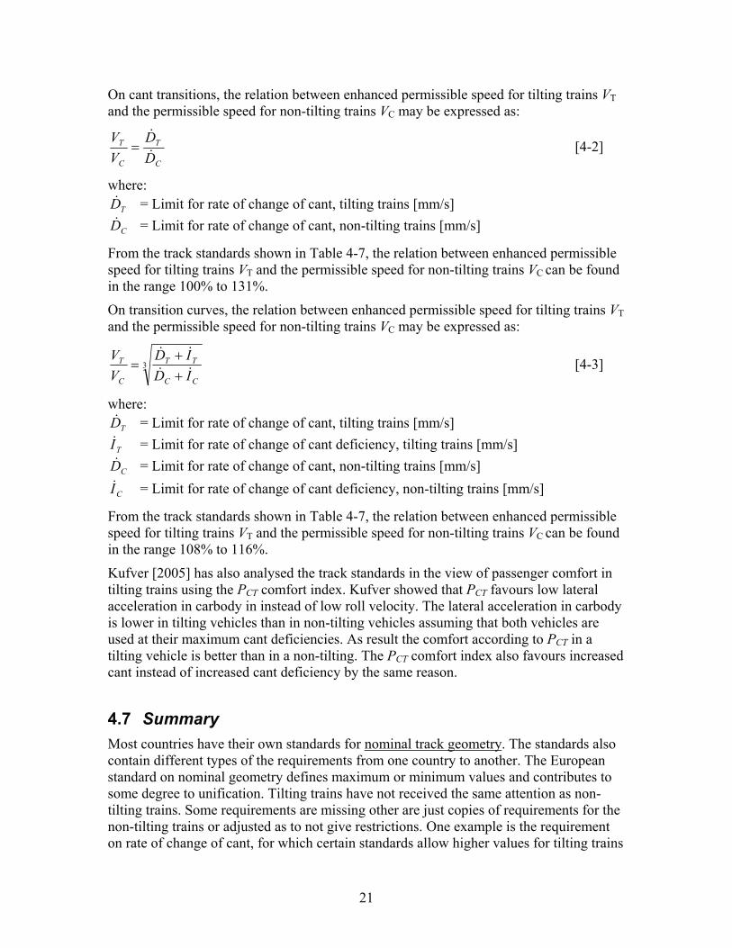
6 Motion sickness ..................................................................................... 37 6.1 Evidence of motion sickness............................................................................. 37 6.2 Hypothesis of motion sickness.......................................................................... 37 6.3 Deriving models of motion sickness................................................................. 38 6.4 Models of motion sickness................................................................................ 40 6.5 Time dependence of motion sickness ............................................................... 41 6.6 Calculation of net doses based on ideal track geometry ................................... 42 6.7 How can motion quantities be limited? ............................................................ 43 6.8 Summary ........................................................................................................... 43

iv

7 Winter properties ................................................................................... 45 7.1 Lift of ballast stones.......................................................................................... 45

7.1.1 The phenomenon ................................................................................................. 45 7.1.2 Countermeasures to lift of ballast stones............................................................. 45

7.2 Snow packing.................................................................................................... 47 7.2.1 The phenomenon ................................................................................................. 47 7.2.2 Countermeasures to snow packing ...................................................................... 47

7.3 Summary ........................................................................................................... 48

Part 2, Analysis ........................................................................................... 49

8 Analysis of vehicle and infrastructure ................................................... 51 8.1 Vehicles............................................................................................................. 51

8.1.1 Availability of tilting trains ................................................................................. 51 8.1.2 Tilt actuator ......................................................................................................... 51

8.2 Infrastructure..................................................................................................... 52 8.2.1 Speed limitations ................................................................................................. 52 8.2.2 Choice of cant...................................................................................................... 53

8.3 Summary ........................................................................................................... 56

9 Analysis of services suitable for tilting trains........................................ 57 9.1 Running time – cant deficiency, top speed or tractive performance................. 57 9.2 Performance of X2000...................................................................................... 57 9.3 Performance of a new tilting train .................................................................... 59

9.3.1 The tracks ............................................................................................................ 59 9.3.2 The trains............................................................................................................. 60 9.3.3 Cant deficiency.................................................................................................... 60 9.3.4 Top speed ............................................................................................................ 62 9.3.5 Tractive power..................................................................................................... 64

9.4 Distance between stops ..................................................................................... 65 9.5 New tracks, for tilting or high-speed trains?..................................................... 67

9.5.1 Background ......................................................................................................... 67 9.5.2 Consequences on capacity caused by different train categories.......................... 69

9.6 Upgrading tracks or tilting trains ...................................................................... 71 9.6.1 Track upgrading .................................................................................................. 71 9.6.2 Cost comparison.................................................................................................. 72

9.7 Summary ........................................................................................................... 72

10 Discussion and conclusions ................................................................... 73 10.1 Discussion......................................................................................................... 73 10.2 Conclusions....................................................................................................... 75 10.3 Suggestions for further research ....................................................................... 76

References..................................................................................................... 77

Annex A. Symbols.................................................................................. A-1

Annex B. Abbreviations ......................................................................... B-1

Annex C. Tilting vehicles that are in or have been in service................ C-1

1

1 Introduction

1.1 Background to the present study Growing competition from other means of transportation has forced railway companies throughout the world to search for increased performance. Travelling time is the most obvious performance indicator that may be improved by introducing high-speed trains. High-speed trains requires straight track or at least tracks with large curve radii and long transition curves not to impair the ride comfort, another performance indicator. Building new tracks with large curve radii is costly and can only be justified where the passenger base is large.

Trains with capability to tilt the bodies inwards the curve is a less costly alternative than building new tracks with large curve radii. The tilt inwards reduces the centrifugal force felt by the passengers, allowing the train to pass curves at enhanced speed with maintained ride comfort. Trains capable to tilt the bodies inwards is often called tilting trains.

Tilting has today become a mature technology accepted by most operators, but not favoured by many. There are different reasons behind this fact; the non-tilting trains have increased their speed in curves (however at a reduced level of ride comfort), reducing the potential for travelling time reduction by tilting trains to approximately 10 -15 %. The popularity is also impacted by low reliability and motion sickness on certain services.

International Union of Railways (UIC) [1998] and [2005b] has reported on Tilting Train technology where tilting trains and known tilting technology are described briefly. This report covers tilting trains and known tilting technology as well as an analysis of the present situation.

1.2 Objective and approach of the present study The objective with this study is to identify areas where the competitiveness of tilting trains can be improved and to conduct further research on identified areas.

The research is divided in two stages with different aims and activities. The aims and activities in a later stage will be depending on the results of earlier stages.

Stage 1 – To make an overview of the present situation on technology, knowledge and

development trends. – To identify areas where research can improve the competitiveness of tilting trains.

Stage 2 – To conduct research on one or more areas identified at stage 1.

2

The present research report summarises stage 1. This report is divided in two main parts, the first, chapters 2 to 7 covers knowledge found in the literature study. Chapters 8 to 10 covers analysis made within this study with the aim to identify areas where research can improve the competitiveness of tilting trains.

3

Part 1, Literature study

5

2 The concept of tilting trains A train and its passengers are subject to centrifugal forces when the train passes horizontal curves. Roll inwards reduces the centrifugal force felt by the passengers allowing the train to pass curves at enhanced speed with maintained ride comfort. Roll may be achieved by track cant, or when the track cant is insufficient, carbody tilt. Trains capable to tilt the bodies inwards is often called tilting trains. The tilting trains can be divided in two groups, the passively tilted trains, called natural tilted trains in Japan, and the actively tilted trains (active tilt is called forced tilt in certain publications).

The passive tilt relies on natural laws with a tilt centre located well above the centre of gravity of the carbody. On a curve, under the influence of centrifugal force, the lower part of the carbody swings outwards. It should be noted that passive tilt has a negative impact on safety due to the lateral shift of centre of gravity of the carbody.

The active tilt relies on active technology, controlled by a controller and executed by an actuator. Tilt as such has normally not an impact on safety on actively tilted train.

The basic concept of tilting trains is the roll of the vehicle bodies inwards the curve in order to reduce the lateral force perceived by the passenger, Figure 2-1.

Track level

Tilt angle

Lateralforce

Track level

Verticalforce

Lateralforce

Verticalforce

Track level

Tilt angle

Lateralforce

Track level

Verticalforce

Lateralforce

Verticalforce

Figure 2-1: The basic concept of tilting trains.

Despite the higher track plane acceleration for the tilting train (right), the lateral force in the carbody is lower.

6

When a vehicle is running on a horizontal curve there will be a horizontal acceleration which is a function of speed v and curve radius R.

Rvah

2

= [2-1]

The acceleration in the track plane can be reduced compared with the horizontal acceleration by arranging a track cant D. The angle between the horizontal plane and the track plane is a function of the track cant and the distance 02 b⋅ between the two contact points of a wheelset.

)2

arctan(0b

Dt ⋅=ϕ [2-2]

The acceleration perceived by the passenger can be further reduced compared with the track plane acceleration by arranging a carbody tilt angle cϕ . The acceleration in the carbody is normally called lateral acceleration and is denoted as y&& . The acceleration in the perpendicular direction is normally called vertical acceleration and is denoted as z&& .

)sin()cos(2

ctct gRvy ϕϕϕϕ +⋅−+⋅=&& [2-3]

)cos()sin(2

ctct gRvz ϕϕϕϕ +⋅++⋅=&& [2-4]

A reduction of lateral acceleration by increased track cant or carbody tilt is correlated with a slightly increased vertical acceleration. Typical values for lateral and vertical acceleration are shown in Table 2-1. Table 2-1: Certain typical values for motion quantities on a horizontal curve

Speed v [km/h]

Radius R [m]

Track cant D [mm]

Carbody tilt angle cϕ [degrees]

Lateral acceleration

y&& [m/s2]

Vertical acceleration z&& [m/s2] 1)

113 1000 0 0 0,98 3) 0

113 1000 150 0 0 0,05

160 1000 150 0 0,98 3) 0,15

166 1000 150 6,5 2) 0 0,23

201 1000 150 6,5 2) 0,98 0,44 1) The vertical acceleration is here given as offset from g 2) This tilt angle corresponds to an actively tilted train 3) The real value is 15 to 30 % higher due to roll in suspensions

7

3 Vehicles

3.1 Tilting trains of the world + trends The first considerations and experiments on reducing the centrifugal force felt by the passenger and thereby allowing higher speeds in curves date from the late 1930s, Deischl [1937] and Van Dorn & Beemer [1938]. In 1938, Pullman built for the Atchison, Topeka and Santa Fe Railway an experimental pendulum coach, but the lack of damping produced a sea-sickness inducing rolling motion, Wikipedia [2006]. The novel designs where based on passive technology. In 1956, Pullman-Standard built two train sets, called Train-X, that become the first tilting trains in commercial service. The trains were withdrawn from service after as short period due to poor running behaviour. The first large series of tilting trains were the Japanese class 381, which started to run between Nagoya and Nagano in 1973. In 1980, the first tilting Talgo train was put into service between Madrid and Zaragoza in Spain. All these trains had passive (or natural) tilt.

Active technology was introduced 1957 when La Société Nationale des Chemins de Fer (SNCF) built a vehicle that could tilt up to 18 degrees. Deutsche Bahn (DB) converted 1965 a diesel multiple unit series 624 for tilt. In 1972 a tilting version of series 624 called series 634 were put into service on the line Cologne – Saarbrucken as the first actively tilted train in commercial service.

One important development chain for the actively tilting trains was the development of the Pendolino trains, which started 1969 with a prototype tilting railcar, the Y0160. The prototype was 1975 followed by ETR401, which become the first Pendolino in commercial service, Figure 3-1.

Figure 3-1: The Italian Railways ETR401, Photo by Paolo Zanin

British Rail gained a lot of experience with their prototype tilting train, the Advanced Passenger Train (APT). One example is the comfort indexes PCT and PDE, which were developed from test with APT, Harborough [1986]. The trains featured a lot of new developments, with the drawback of poor reliability. The project was finally abandoned, and some patents were sold to FIAT which applied the knowledge on the later introduced ETR450.

8

The break-through for actively tilted trains came around 1990 when introduction of large series, like the ETR450 in Italy and the X2000 in Sweden, started. At the same time the series 2000 trains were introduced in Japan, which were the first natural tilted trains with active tilt support. Today more than 5000 tilting vehicles, defined as tilting carbodies, have been produced world-wide by different suppliers. Table 3-1, gives a list of, for the development tilt, certain important vehicles, a list of tilting vehicles that are in or have been in service is found in Appendix B. Table 3-1: Certain important vehicles in the development of tilt technology Developer Product Year Top

speed[km/h]

Tilt actuation

Comment

Pullman – Standard 1)

Train-X 1956 ? Passive First tilting vehicle in service

SNCF - 1957 ? ? First vehicle with active tilt FS/FIAT Y0160 1969 200 Hydraulic First vehicle of FIAT

technology DB 634 1972 140 Pneumatic First vehicle with active tilt in

service BR APT-E 1972 240 Hydraulic The comfort indexes PCT and

PDE were developed JR/Hitachi 381 1973 120 Passive First vehicle on Hitachi

technology FS/FIAT ETR401 1975 171 Hydraulic First vehicle of FIAT

technology in service SJ/ASEA X15 1975 200 Pneum. /

Hydraulic First vehicle of ASEA

technology Talgo Pendular 1980 180 Passive First tilting Talgo FS/FIAT ETR450 1989 250 Hydraulic Highest top speed of trains in

service JR/Hitachi 2000 1989 130 Passive +

PneumaticFirst vehicle using stored

track data

ASEA/ABB X2000 1990 200 Hydraulic First vehicle of ASEA technology in service

AEG VT611 1997 160 El-Mech. First vehicle with electro-mechanical actuators

JR/Hitachi N700 2007? 300 Pneumatic First tilting vehicle in service with top speed above

250 km/h? 1) The design was based on a Talgo patent

9

The early developments on actively tilting trains in Europe were initiated by the operators like SNCF and DB. In the late 60s, Ferrovie dello stato (FS) joined forces with FIAT that led to the construction of a prototype tilting railcar, the Y0160, which is the predecessor of the Pendolino. Swedish State Railways (SJ) and ASEA had a joint venture with the X15, which gave the tilting technology to X2000. Today most train development is performed by the suppliers, a statement also valid for tilting trains. In fact, the tilt technology has become that mature that the development has been partly transferred to the sub-suppliers, like Extel Systems Wedel (ESW) and Curtiss-Wright which supplies tilt systems based on electro-mechanical actuators.

The request for performance of trains has generally led to increased maximum speeds. The tilting trains are following this trend. The first tilting trains had a maximum speed of 120 km/h in service. Narrow gauge trains in Japan have still only 130 km/h as maximum speed, when the tilting trains in Europe have at least 160 km/h as maximum speed. The Acela trains in USA has 240 km/h as top speed, but still the Pendolino trains, ETR450, ETR460 and ETR480 in Italy have the highest maximum speed of all tilting trains in service, 250 km/h, see Figure 3-2. However, the Italian tilting trains runs at the same speed as Italian non-tilting trains at speeds above 200 km/h, Casini [2005]. Research on trains, which combines top speeds higher than 250 km/h and tilting capability, has been performed by SNCF/Alstom (tilting TGV) and JR/Hitachi (tilting Shinkansen series N700). The latter is planned to enter service 2007 with a top speed of 300 km/h, a maximum cant deficiency of 154 mm and a maximum tilt angle of 1 °.

0

50

100

150

200

250

300

1970 1980 1990 2000 2010

1st year in service

Max

imum

ser

vice

spe

ed [k

m/h

]

Figure 3-2: Top speed as function of 1st year of service

10

3.2 Tilt technology and trends Two parallel development chains may be seen in tilt technology, one based on passive or natural tilt as it is called in Japan and one on active tilt. The passive tilt relies on natural laws with a tilt centre located well above the centre of gravity of the carbody. On a curve, under the influence of the centrifugal force, the lower part of the carbody swings outwards. The designer must consider the trade-off between damping (i.e. small “swinging” motions) and fast response. The series 2000 trains in Japan was the first train were active tilt support where added to a passively tilted train to enhance performance.

Some of the first actively tilting trains relied on active technology based on pneumatic systems, where air was shifted from one side to the other of the air suspension. An important technology step come with rollers and pendulums which carry the carbody load and provide movement possibility. The movement may then be controlled by an actuator that not has to carry the carbody load, resulting in much lower energy consumption.

Hydraulic actuators were introduced by FS/FIAT in Y0160, where they proved their capability. These systems consist of cylinders, placed in or in connection to the bogie, and a hydraulic power pack with motor, pump, valves etc. placed in the underframe of the carbody. The electro-mechanical actuators showed advantages and become an alternative in 1990s. These systems consist of actuators placed in the bogie and an electric power pack with converter placed in the underframe of the carbody, Figure 3-3.

Figure 3-3: Electromechanical actuator, ESW [2006]

The electro-hydraulic actuator becomes an alternative in the next generation of tilting trains. These systems consist of the same components as the electro-mechanical actuator, but the mechanical gear in the actuator is replaced by a pump and a cylinder, Enomoto [2005].

The actively tilted trains need some kind of control system. Novel systems applied a body feedback with an accelerometer placed in the carbody as transducer. The body feedback systems had stability problems due to low-frequency movements in the secondary suspension, forcing development of the bolster feedback systems. The bolster feedback systems uses transducers placed in the tilted part of the bogie. A reference transducer in the non-tilted part of the bogie give the advantage of allowing partial compensation of the lateral acceleration, Figure 3-4, which have an positive impact on motion sickness, Förstberg [2000].

11

Controller Actuator Body

Body accelerometer

Body feedback

Controller Actuator BodyBogieaccelerometer

Referencetransducer

Position transducer

Bolster feedbackController Actuator Body

Bogie accelerometer

Controller Actuator Body

Body accelerometer

Body feedback

Controller Actuator BodyBogieaccelerometer

Referencetransducer

Position transducer

Bolster feedbackController Actuator Body

Bogie accelerometer

Figure 3-4: Block diagram of tilting system layouts

There are different kinds of information sources that can be used as reference transducer. The obvious one is the lateral acceleration, but also roll and yaw velocity may be used. Most tilting trains use more than one source as base for its control. The typical nominal behaviour of these signals is shown in Figure 3-5.

Circular curveTransitioncurve

Transitioncurve

Lateral acceleration

Yaw velocity

Roll velocity

Circular curveTransitioncurve

Transitioncurve

Lateral acceleration

Yaw velocity

Roll velocity

Figure 3-5: Information sources and their typical behaviour

Assuming that the speed is constant the sources have following properties:

1. Lateral acceleration measured in the bogie has a close relation to the cant deficiency at track level. The lateral acceleration changes on transition curves and receives a constant value on the circular curve. The lateral acceleration can in principle be used directly as a lead value base.

12

2. Yaw velocity measured in the bogie has a relation to curve radius and speed. The yaw velocity changes in transition curves and receives a constant value in the circular curve. The relation to curve radius and speed means that the cant and speed must be considered before yaw velocity can be used as lead value base.

3. Roll velocity measured in the bogie has a relation to the rate of change of cant of the track. The roll velocity receives a non-zero value in the cant transition when the installed cant changes and a zero in the circular curve when the installed cant is kept constant. The roll velocity is an excellent indicator of cant transitions, which may be used to switch between different control strategies.

All three sources have zero value on straight track.

Japanese tilting trains uses wayside information to improve the performance. The system is combined with the Automatic Train Protection (ATP) system, where timing information is send from a way-side element to the ATP system in the train and further to the tilt controller. The track data is stored on board the train. The Spanish supplier Construcciones y Auxiliar de Ferrocarriles (CAF) has in series R-598 showed that a system based on stored track data can work without wayside input, Gimenez & Garcia [1997]. The stored track data can either be based on a track data register or on train measured track data. A positioning system is needed to pick the right track data at the right time.

Sasaki [2005] give four different information sources to the positioning system: 1. Way-side beacons 2. Global Positioning System (GPS) and comparison with line map 3. Comparing the measured curvature with line data 4. Integrating the speed signal.

Sasaki show how sources 2 to 4 can be combined with 1. All four sources can be used together by selection the best source at each moment. The accuracy has been tested and found to better than 4 metres, the accuracy for the GPS alone was 34 meters. 10 metres accuracy is assumed by Sasaki as limit for tilting timing purpose.

3.3 Summary Tilting trains can today be purchased from all the major train suppliers. The top speed of tilting trains follows the trend towards higher speeds. The first tilting train with top speed above 250 km/h will be set into service in 2007 in Japan, the Shinkansen N700. It should be noted that the maximum cant deficiency will be similar to Swedish non-tilting passenger trains.

Different means of actuation exists for the active carbody tilt, different suppliers prefer different solutions. Common is that actuation can be bought from sub-suppliers. Control systems using stored track data has entered the market and this is a trend that likely will continue.

13

4 Track

4.1 Design track geometry, terms and definitions Track gauge Track gauge is the distance between the inner faces of the rail heads of the track. The track gauge is measured 14 mm below the top of the rail on the inner face. Standard track gauge is 4 feet, 8-1/2 inches or approximately 1435 mm.

Circular horizontal curve Circular horizontal curve is a curve in the horizontal plane with constant radius. The circular horizontal curve is characterized by its radius R which is related to the track centre line. The circular horizontal curve may also be characterized by its curvature which the inverse to the radius.

Transition curve Transition curves are used to connect straight track to circular horizontal curves or to connect two circular horizontal curves. The transition curve is characterized by its curvature as function of the longitudinal position. The most common transition curve has linear variation of the curvature; this type of transition curve is called clothoid.

Track cant Track cant D (or superelevation) is the amount one running rail is raised above the other running rail (in a curve). Track cant is positive when the outer rail is raised above the inner rail.

Cant transitions Cant transitions (or superelevation ramps) are used to connect two different track cants. The cant transition has in most cases the same longitudinal position as the transition curve. The cant gradient is characterized by its longitudinal distance to raise one unit (normally expressed as 1 in X, where X is the longitudinal distance in units). The most common cant transition has a linear variation of the track cant.

Rate of change of cant Rate of change of cant is the rate of which cant is increased or decreased at a defined speed. The rate of change of cant is characterized by the cant change per time unit

dtdD / . The most common cant transition has constant rate of change of cant.

Cant deficiency Cant deficiency I arises when the installed cant is lower than the cant of equilibrium. The cant deficiency is characterized by the additional cant needed to receive equilibrium.

Rate of change of cant deficiency Rate of change of cant deficiency is the rate of which cant deficiency is increased or decreased at a defined speed. The rate of change of cant deficiency is characterized by the cant deficiency change per time unit dtdI / . The most common transition curve / cant transition has constant rate of change of cant deficiency.

14

Track gradient Track gradients are used to connect tracks at different altitudes. The track gradient is normally characterized in per mille (or per cent), but in certain countries as longitudinal distance to raise one unit (normally expressed as 1 in X, where X is the longitudinal distance in units).

Vertical curve Vertical curves are used to connect two different track gradients. Vertical curves are normally circular curves. The vertical curve is characterized by its radius Rv. The design track geometry properties described above have impacts on safety and ride comfort, these relations are described in Table 4-1 and 4-2. Table 4-1 Design track geometry relation to safety

Property Relation to safety

Track gauge The track gauge has an impact on the lateral behaviour of the vehicle which may lead to unstable running.

Circular horizontal curve Reduced circular horizontal curve radius increases the lateral track forces, which increases the derailment ratio (Y/Q).

Transition curve No impact

Track cant High cant may be a problem for freight wagons where brake to stop at high cant may shift the load. UIC has proved that 180 mm is acceptable.

Cant transitions Steep cant transitions may lead to diagonal wheel unloading which in turn may lead to derailment due to flange climbing. European Rail Research Institute (ERRI) has showed that 1/400 m/m is acceptable.

Rate of change of cant No impact (see cant transitions)

Cant deficiency High cant deficiency may lead to high lateral track forces. High cant deficiency also increases the risk of over-turning.

Rate of change of cant deficiency No impact

Track gradient No impact

Vertical curve No impact Note: No impact means that no first order dependences exist.

15

Table 4-2 Design track geometry relation to ride comfort

Property Relation to ride comfort

Track gauge The track gauge has an impact on the lateral behaviour of the vehicle which has an impact on the lateral ride comfort.

Circular horizontal curve No impact (see cant deficiency)

Transition curve Reduced transition curve length increases rate of change of cant deficiency and thereby also the lateral jerk perceived by the passenger. It also increases the roll velocity for tilting trains, which is believed to contribute to motion sickness.

Track cant No impact (see cant deficiency)

Cant transitions No impact (see rate of change of cant)

Rate of change of cant Increased rate of change of cant increases the roll velocity perceived by the passenger. Roll velocity is considered to contribute to motion sickness.

Cant deficiency Increased cant deficiency increases the lateral carbody acceleration perceived by the passenger.

Rate of change of cant deficiency Increased rate of change of cant deficiency increases the lateral jerk perceived by the passenger. It also increases the roll velocity in tilting vehicles. Roll velocity is considered to contribute to motion sickness for tilting vehicles.

Track gradient No impact

Vertical curve No impact Note: No impact means that no first order dependences exist.

4.2 National standards in Sweden The national standards in Sweden, issued by BV, gives guidance on cant, cant gradient, cant deficiency, rate of change of cant and rate of change of cant deficiency for non-tilting vehicles as well as tilting vehicles, BV [1996]. The standard also gives guidance on vertical curves. The standard is under revision, 2006. Certain key requirements are given in Table 4-3. The Swedish standard categorizes the trains based on running gear and tilting capability: A Non-tilting trains B Non-tilting trains equipped with running gear for high cant deficiency service. S Tilting trains equipped with running gear for high cant deficiency service.

16

Table 4-3: Key requirements for tilting trains in Sweden

Cant [mm] Rate of change of cant [mm/s]

Cant deficiency [mm]

Rate of change of cant deficiency

[mm/s]

150 60 1) 245 79 1) The official value is 69 mm/s but due to other limits the rate of change of cant does not

exceed 60 mm/s.

4.3 Standards of European committee of standardization The European committee of standardization (CEN), gives guidance on cant, cant gradient, cant deficiency, rate of change of cant and rate of change of cant deficiency for non-tilting vehicles, CEN [2002]. The standard also gives guidance on vertical curves. The standard is under revision, tilting vehicles are considered in working draft version CEN [2006b]. Certain key requirements are given in Table 4-4.

The CEN-standards categorize the track based on the type of services on the track: I Mixed traffic lines, with passenger train speeds from 80 km/h to 120 km/h II Mixed traffic lines, with passenger train speeds greater than 120 km/h and up to

200 km/h III Mixed traffic lines, with passenger train speed higher than 200 km/h IV Mixed traffic lines, for vehicles incorporating special technical design

characteristics V Dedicated passenger lines with speed over 250 km/h

Table 4-4: Key requirements for tilting trains according to CEN [2006b]

Cant [mm] Rate of change of cant [mm/s]

Cant deficiency [mm]

Rate of change of cant deficiency

[mm/s]

180 1) 75 306 150 1) For mixed traffic lines, for vehicles incorporating special technical design characteristics

4.4 Technical Specifications of Interoperability European Association for Railway Interoperability (AEIF), gives in The Technical Specifications of Interoperability (TSI) for Trans-European High-Speed Rail system, Infrastructure guidance on cant and cant deficiency for non-tilting vehicles, AEIF [2002a]. No guidance is given for tilting trains (infrastructure owner may decide).

AEIF categorize the track based on the type of services on the track, they are: I Lines especially built for high speed. II Lines especially upgraded for high speed. III Lines especially built or upgraded for high speed having special features.

17

The cant is maximized to 180 mm for all lines, when the maximum cant deficiency is depending on track category and speed, see Figure 4-1.

0

50

100

150

200

0 100 200 300 400Speed [km/h]

Can

t def

icie

ncy

[mm

]

Upgraded lines, High performance vehiclesUpgraded linesHigh Speed Lines

Figure 4-1: Maximum cant deficiency for non-tilting vehicles as function of speed,

AEIF [2002a]

4.5 Track irregularities Track irregularities are deviations from the nominal track geometry. Requirements on track irregularities are divided in maximum deviation from mean (mean-to-peak) and standard deviation. The maximum values are safety-related and the standard deviation has a relation to ride comfort.

The national standards in Sweden, issued by BV [1997], give guidance on track irregularities as maximum deviation from mean (mean-to-peak) and standard deviation. Explicit guidance is given for track irregularities with long wave lengths and tracks used by tilting vehicles.

CEN has not issued any standard for track irregularities; but work is in progress within WG28 2006. AEIF [2002a] gives guidance on track irregularities as maximum deviation from mean (mean-to-peak) and standard deviation. No guidance for track irregularities longer than 25 m is given. Tilting vehicles are not considered explicitly in this standard.

A comparison on track irregularities (as mean-to-peak) between BV [1997] and AEIF [2002a] is shown in Table 4-5. The limits on track irregularities are depending on speed. The levels of track irregularities are valid within specified speed intervals, which are different from standard to standard, and the values in the table are therefore given at selected speeds to allow comparison. BV, but not AEIF, differentiates between non-tilting vehicles and tilting vehicles, the values shown are for tilting vehicles. Both BV and AEIF differentiate between requirements for planned maintenance and unplanned maintenance.

18

Table 4-5 Track irregularities, BV and AEIF, mean to peak BV AEIF Maintenance level Planned Unplanned Planned 2) Unplanned Vertical [mm] (3 to 25 m wave lengths) 1)

at V = 120 km/h 10 16 8 12 at V = 160 km/h 6 10 6 10 at V = 200 km/h 6 9 5 9 at V = 300 km/h NA NA 4 8

Vertical [mm] (25 to 100 m wave lengths) at V = 120 km/h - - - - at V = 160 km/h 15 - - - at V = 200 km/h 15 - - - at V = 300 km/h NA NA - -

Lateral [mm] (3 to 25 m wave lengths) 1) at V = 120 km/h 6 10 8 10 at V = 160 km/h 4 6 6 8 at V = 200 km/h 3 5 5 7 at V = 300 km/h NA NA 4 6

Lateral [mm] (25 to 100 m wave lengths) at V = 120 km/h - - - - at V = 160 km/h 10 - - - at V = 200 km/h 10 - - - at V = 300 km/h NA NA - -

Cross level [mm] (on 3 m longitudinal base) at V = 120 km/h 9 13 - 10,5 at V = 160 km/h 7 10 - 10,5 at V = 200 km/h 6 9 - 7,5 at V = 300 km/h NA NA - 7,5

Gauge [mm] at V = 120 km/h 1430 –

1450 1430 – 1465

- -

at V = 160 km/h 1430 – 1442

1430 – 1455

- -

at V = 200 km/h 1430 – 1440

1430 – 1450

- -

at V = 300 km/h NA NA - 1434 – 1443

1) BV uses the wave length interval 1 – 25 m, AEIF does not specify the wave length but the values are the same as in CEN [2005] standard for vehicle homologation which specify the wave length to 3 – 25 m.

2) The values are given as information by AEIF, same as given in CEN [2005] standard for vehicle homologation.

19

A comparison between BV [1997] and AEIF [2002a] on track irregularities as standard deviation is shown in Table 4-6. The limits on track irregularities are depending on speed. The levels of track irregularities are valid within specified speed intervals, which are different from standard to standard, and the values in the table are therefore given at selected speeds to allow comparison. BV differentiates between non-tilting vehicles and tilting vehicles, the values shown are for tilting vehicles. BV has only requirements for planned maintenance. Table 4-6 Track irregularities, BV and AEIF, standard deviation BV AEIF Quality level Planned Unplanned Planned 2) Unplanned Vertical [mm] (3 to 25 m wave lengths) 1)

at V = 120 km/h 1,9 - 1,8 2,1 at V = 160 km/h 1,3 - 1,4 1,7 at V = 200 km/h 1,1 - 1,2 1,5 at V = 300 km/h NA - 1,0 1,3

Lateral [mm] (3 to 25 m wave lengths) 1) at V = 120 km/h 1,7 - 1,2 1,5 at V = 160 km/h 1,2 - 1,0 1,3 at V = 200 km/h 1,1 - 0,8 1,1 at V = 300 km/h NA - 0,7 1,0

Cross level [mm] (on 3 m longitudinal base) at V = 120 km/h 1,4 - - - at V = 160 km/h 1,0 - - - at V = 200 km/h 0,9 - - - at V = 300 km/h NA - - - 1) BV uses the wave length interval 1 – 25 m, AEIF does not specify the wave length but

the values are the same as in CEN [2005] standard for vehicle homologation which specify the wave length to 3 – 25 m.

2) The values are given as information in AEIF [2002a], same as given in CEN [2005] standard for vehicle homologation.

4.6 Analysis of track geometry Kufver has within the Fast And Comfortable Trains (FACT) project analysed the track standards in the view of tilting trains, Kufver [2005]. Relations between enhanced permissible speed for tilting trains and the permissible speed for non-tilting trains are expressed for different track segments.

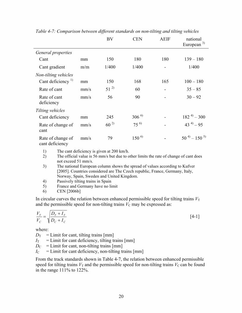
The different track standards show a large spread in requirements, which can be seen in Table 4-7 where certain key requirements from different standards are given.

20

Table 4-7: Comparison between different standards on non-tilting and tilting vehicles

BV CEN AEIF national European 3)

General properties Cant mm 150 180 180 139 – 180

Cant gradient m/m 1/400 1/400 - 1/400

Non-tilting vehicles Cant deficiency 1) mm 150 168 165 100 – 180

Rate of cant mm/s 51 2) 60 - 35 – 85

Rate of cant deficiency

mm/s 56 90 - 30 – 92

Tilting vehicles Cant deficiency mm 245 306 6) - 182 4) – 300

Rate of change of cant

mm/s 60 2) 75 6) - 43 4) – 95

Rate of change of cant deficiency

mm/s 79 150 6) - 50 4) – 150 5)

1) The cant deficiency is given at 200 km/h. 2) The official value is 56 mm/s but due to other limits the rate of change of cant does

not exceed 51 mm/s. 3) The national European column shows the spread of values according to Kufver

[2005]. Countries considered are The Czech republic, France, Germany, Italy, Norway, Spain, Sweden and United Kingdom.

4) Passively tilting trains in Spain 5) France and Germany have no limit 6) CEN [2006b]

In circular curves the relation between enhanced permissible speed for tilting trains VT and the permissible speed for non-tilting trains VC may be expressed as:

CC

TT

C

T

IDID

VV

++

= [4-1]

where: DT = Limit for cant, tilting trains [mm] IT = Limit for cant deficiency, tilting trains [mm] DC = Limit for cant, non-tilting trains [mm] IC = Limit for cant deficiency, non-tilting trains [mm]

From the track standards shown in Table 4-7, the relation between enhanced permissible speed for tilting trains VT and the permissible speed for non-tilting trains VC can be found in the range 111% to 122%.

21

On cant transitions, the relation between enhanced permissible speed for tilting trains VT and the permissible speed for non-tilting trains VC may be expressed as:

C

T

C

T

DD

VV

&

&= [4-2]

where: TD& = Limit for rate of change of cant, tilting trains [mm/s]

CD& = Limit for rate of change of cant, non-tilting trains [mm/s]

From the track standards shown in Table 4-7, the relation between enhanced permissible speed for tilting trains VT and the permissible speed for non-tilting trains VC can be found in the range 100% to 131%.

On transition curves, the relation between enhanced permissible speed for tilting trains VT and the permissible speed for non-tilting trains VC may be expressed as:

3

CC

TT

C

T

IDID

VV

&&

&&

++

= [4-3]

where: TD& = Limit for rate of change of cant, tilting trains [mm/s]

TI& = Limit for rate of change of cant deficiency, tilting trains [mm/s]

CD& = Limit for rate of change of cant, non-tilting trains [mm/s]

CI& = Limit for rate of change of cant deficiency, non-tilting trains [mm/s]

From the track standards shown in Table 4-7, the relation between enhanced permissible speed for tilting trains VT and the permissible speed for non-tilting trains VC can be found in the range 108% to 116%.

Kufver [2005] has also analysed the track standards in the view of passenger comfort in tilting trains using the PCT comfort index. Kufver showed that PCT favours low lateral acceleration in carbody in instead of low roll velocity. The lateral acceleration in carbody is lower in tilting vehicles than in non-tilting vehicles assuming that both vehicles are used at their maximum cant deficiencies. As result the comfort according to PCT in a tilting vehicle is better than in a non-tilting. The PCT comfort index also favours increased cant instead of increased cant deficiency by the same reason.

4.7 Summary Most countries have their own standards for nominal track geometry. The standards also contain different types of the requirements from one country to another. The European standard on nominal geometry defines maximum or minimum values and contributes to some degree to unification. Tilting trains have not received the same attention as non-tilting trains. Some requirements are missing other are just copies of requirements for the non-tilting trains or adjusted as to not give restrictions. One example is the requirement on rate of change of cant, for which certain standards allow higher values for tilting trains

22

than for non-tilting vehicles. A requirement on rate of change of cant can possibly be logical for a non-tilting vehicle where a direct relation to roll velocity exists, but on the other hand, the roll velocity is much higher in a tilting vehicle.

The work with a European standard on deviations from nominal geometry (i.e. track irregularities) has started and may contribute to unification; today some of this information is found in standards for vehicle homologation, CEN [2005]. Requirements on longer wave lengths than 25 meters should be stated. The roll motions of vehicles should be considered when selecting the upper limit for wave lengths.

23

5 Track – vehicle interaction The track–vehicle interaction is today guided by standards. In Europe these standards are issued by CEN, some based on a UIC-standard. These standards are widely used also outside Europe. Comparison with older vehicles is another possibility to set limits. This technique was applied when SJ set certain limits for the tilting train that became X2000. Today this type of limits is found in TSI for high-speed trains on the task of side wind stability issued by AEIF [2006].

5.1 Track forces

5.1.1 Methods CEN [2005] gives guidance on track shift forces, derailment ratio, lateral wheel forces and vertical wheel forces, Figure 5-1. The same properties with the same limit values are found in UIC [2005a]. Both these standards are for vehicle homologation where the stipulated requirements set the limits to be accepted. The track forces are normally measured with measuring wheelsets. The standards also give guidance on how to select suitable track sections for the measurements and how to process the measured forces. Low-pass filtering is one part of the process, where both standards allow 20 Hz as cut-off frequency. Frequencies higher than the cut-off frequency are not considered. Statistical treatment is made in two steps, the first step considers the value over one test section (70 to 500 meter) the second step combines different test sections to test zones (test zone here means straight track, large curve radius or small curve radius).

Yr

Yl

Qr

QlΣY = Yr + Yl

Yr

Yl

Qr

QlΣY = Yr + Yl

Figure 5-1: Definitions of track forces

Track shift force The track shift force is the sum of lateral wheel forces on a wheelset, ∑Y in Figure 5-1. The track shift force is related to the risk of shifting the track laterally when a train passes. The criterion is also known as the Prod´homme criterion after the inventor, Prod´homme [1967]. The track shift force is considered as safety critical.

24

The track shift force is taken as a two-meter average. The considered value over a test section is the 99,85% value. The considered value over a test zone is the 99% confidence value, which is compared with the limit:

)3210( 01limmax, QkY ⋅+⋅=Σ [kN] [5-1]

where: k1 is a constant equal to 1 for all vehicles except freight wagons Q0 is the static vertical wheel load [kN]

The track shift force can be divided in two parts, one quasi-static part and one dynamic part. The quasi-static part has a dependence on cant deficiency, which for a tilting train is higher than for a non-tilting train. The dynamic part has a dependence on speed, which (for the same curve radius) is also higher for a tilting train than for a non-tilting train. Important factors for maintaining the track shift forces under the specified limits are, Andersson & Halling [1999]:

- Low nominal loads - Low unsprung mass (impact on dynamic part) - Suspension characteristics (impact on dynamic part) - Radial steering (impact on force distribution between two axles in a bogie)

Derailment criteria The ratio between lateral and vertical track forces on a wheel is used as derailment criterion, this ratio is also called flange climbing criterion. The lateral force on the flange is here balanced to the vertical force at the same wheel. Flange climbing is safety critical.

The derailment criterion is taken as a two-meter average. The considered value over a test section is the 99,85% value. The considered value over a test zone is the 99% confidence value, which is compared with the limit:

8.0limmax,

=⎟⎠⎞⎜

⎝⎛

QY [5-2]

where: Y is the lateral wheel force Q is the vertical wheel force

The derailment ratio can be divided in two parts, one quasi-static part and one dynamic part. The quasi-static part has a dependence on cant deficiency, which for a tilting train is higher than for a non-tilting train, but both the lateral and vertical forces increases when the cant deficiency increases. However, the risk for derailment is higher at low speeds, where the tilt normally is inactive, than in high speeds due to the impact from small curve radii and worse track irregularities, making tilting train no different from the non-tilting train.

25

Lateral wheel-rail forces The lateral wheel-rail forces have a relation to track loading and track maintenance. The lateral track force is divided in two parts, one quasi-static part and one dynamic part. The standards have only limit criterion on the quasi-static part. The criterion is evaluated is small radius curves with radii equal or greater than 250 meter.

The considered value over a test section is the average value. The considered value over a test zone is the average of all curves in the same direction, which is compared with the limit:

( ) 60lim, =qstY [kN] [5-3]

where: Y is the lateral wheel-rail force

The quasi-static part has a dependence on cant deficiency, which for a tilting train is higher than for a non-tilting train. The dynamic part has a dependence on speed, which also is higher for a tilting train than for a non-tilting train. Important factors for maintaining the lateral forces under the specified limits are, Andersson & Halling [1999]:

- Low nominal loads - Low unsprung mass (impact on dynamic part) - Suspension characteristics (impact on dynamic part) - Radial steering (at under-radial steering the creep/friction forces on the low wheel

forces the wheelset towards the high rail, thus increasing the high rail lateral force)

Vertical wheel-rail forces The vertical wheel-rail forces have a relation to track loading and track maintenance. The vertical track force is divided in two parts, one quasi-static part, which includes the static wheel load, and one dynamic part, the standards have limit criteria on both.

The considered value over a test section is the average value. The considered value over a test zone is the average of all curves, which is compared with the limit:

( ) 145lim, =qstQ [kN] [5-4]

where: Q is the vertical wheel force

The considered value over a test section is the 99,85% value. The considered value over a test zone is the 95% confidence value, which is compared with the limit:

( ) 0limmax, 90 QQ += [kN] [5-5a]

where: Q is the vertical wheel force and Q0 the static vertical wheel load [kN]

26

There is also a limit depending on the maximum service speed of the vehicle, at 250 km/h:

( ) 180limmax, =Q [kN] [5-5b]

The quasi-static part has a dependence on cant deficiency, which for a tilting train is higher than for a non-tilting train. The dynamics part has a dependence on speed, which also is higher for a tilting train than for a non-tilting train. Important factors for maintaining the vertical forces under the specified limits are, Andersson & Halling [1999]:

- Low nominal loads - Low unsprung mass (impact on dynamic part) - Suspension characteristics (impact on dynamic part) - Height of centre of gravity

5.1.2 Analysis Kufver [2000] and Lindahl [2001] have simulated track-vehicle interaction for high-speed tilting vehicles with following data, Table 5-1. Table 5-1 Vehicle properties used by Kufver and Lindahl Property Kufver Lindahl

Carbody length 24,95 [m] 25 [m]

Carbody height 3,8 [m] 3,6 [m]

Bogie centre distance 17,7 [m] 18 [m]

Bogie wheel base 2,9 [m] 2,7 [m]

Carbody mass 32 411 [kg] 33 000 [kg]

Carbody centre of gravity height 1,61 [m] 1,55 [m]

Bogie frame mass 5 420 [kg] 6 000 [kg]

Wheelset mass 1 340 [kg] 1 600 [kg]

Both Kufver and Lindahl found that track shift forces can be safety critical for tilting vehicles at high speed. At 360 km/h Lindahl set the maximum allowed cant deficiency to 275 mm in track shift point of view when assuming track irregularities of today’s 200 km/h track in Sweden. An adjusted track standard must be considered for 275 – 300 mm cant deficiency, in particular at speeds higher than 200 km/h.

27

5.2 Wheel / rail wear

5.2.1 Methods Wheel and rail wear may in a general sense be understood as deterioration of the surfaces on wheel and track. This deterioration can be divided in two groups of basic mechanisms, loss of material, i.e. abrasive wear, and Rolling Contact Fatigue (RCF), Kimura [2000].

The wheel and rail wear has a strong relation to economy both for the infrastructure owner and the train operator. The relations between track and train properties are complicated when it comes to wheel and rail wear, nor does it exist any standards that guides in the area. Some train operators set requirements on wheel turning intervals, which often leads to an extensive and complicated verification process due to the number of factors that affects the wheel turning interval.

Enblom [2003] has observed two different models for loss of material: 1. The one-parameter model according to McEven and Harvey [1985] which

assumes a relation between loss of material and the dissipated energy in the contact between wheel and rail.

2. The two-parameter model according to Archard [1953] which assumes a relation between loss of material to contact pressure and sliding velocity.

In the 1980s laboratory studies were made at the Illinois Institute of Technology, which studied material loss under different conditions and suggesting a one-parameter model for wear prediction in curves, Formula 5-6. ν⋅F (named γT in UK) is introduced in some of the most common software packages for vehicle dynamic simulation as the wear number (W). Up till now there is no established method for measuring the wheel wear number.

KA

FkW w +⋅

⋅=ν [5-6]

where: wk = Wear coefficient

F = Tangential creep force V = Creep ratio A = Contact area K = Constant

Rolling contact fatigue is an area where much research is in progress. Ekberg et al [2002] has taken an engineering approach to the problem developing three rolling contact Fatigue Indexes (FI) depending on initiating location. Fatigue is predicted to occur if one or more inequalities are fulfilled.

28

1. Surface initiated fatigue

03

2>

⋅⋅⋅⋅⋅

−=z

surf FkbaFI πμ [5-7a]

2. Sub-surface initiated fatigue

eEQreshDVz

sub aba

FFI ,,2 )1(

4σσμ

π>⋅+−⋅

⋅⋅⋅= [5-7b]

3. Fatigue initiated at deep defects

thzdef FFFI −= [5-7c] where: μ = utilized friction coefficient a, b = axis of the Hertzian contact patch k = yield stress in pure shear

zF = vertical load magnitude DVa = material parameter

resh,σ = hydrostatic part of residual stress eEQ ,σ = equivalent stress fatigue limit

thF = threshold of force magnitude

Burstow [2004] has shown that the wear number can be useful when judging the risk of RCF also, Figure 5-2. The RCF damage is zero for Tγ less than 15 N because the energy can be transmitted to the rail without causing any damage. At 15 N the energy becomes large enough to initiate cracks, at 65 N the energy is so high that wear begins and at 175 N the wear and RCF crack initiating rate is in balance.

Figure 5-2: RCF damage as function of wear number, Tγ, Burstow [2004]

29

5.2.2 Analysis The wheel and rail wear in curves has a relation to the vehicle’s ability of radial steering. This could be achieved by reducing the primary suspension stiffness in longitudinal direction, a technique applied for example in Sweden since the 1980s. Reduced primary suspension stiffness in longitudinal direction may and has been applied on tilting vehicles. Negotiating curves at high cant deficiencies may influence wheel wear due to the increased lateral force that must be taken up by the wheels. However, the increased lateral force is normally accomplished by a decreased angle of attack for the leading wheelset, thus producing a tendency towards reduced wear. The total effect of higher cant deficiency on wheel and rail wear is therefore small regarding wear. Some reports on wheel wear problems on tilting trains are found in the literature, Nationalcorridors [2006] has reported excessive wheel (flange) wear on ICE-T and Trainweb [2006] has reported the same for Acela. None of these vehicles is believed to have any substantial radial steering ability.

From a vehicle point of view, the wheel profile development must also be considered. Flange wear leads to decreased flange thickness and need for reprofiling due to thin flange. Tread wear may lead to high equivalent conicity and a need for reprofiling due to poor running behaviour. The longest wheel turning interval is received when flange wear and tread wear is in balance with each other. However, these phenomenon are not specific for tilting trains only.

RCF has, for all models described by Ekberg et al [2002], a dependence on vertical force magnitudes. The increased cant deficiency will result in increased vertical load on the curve outer wheel, which will increase the risk for RCF. The increased vertical load on the curve outer wheel can be counteracted by modest axle load and low centre of gravity. The risk of RCF may also be counteracted by careful optimization of the utilized friction coefficient. Important ingredients are brake blending and longitudinal primary suspension stiffness.

5.3 Passenger ride comfort

5.3.1 Methods The comfort of passengers in a railway vehicle is influenced by a number of different factors like temperature, noise, vibration etc. The passenger comfort considered here is the part influenced by dynamic behaviour of the vehicle. Passenger comfort in this sense can be divided in three groups:

• Frequency weighted accelerations as functions time, • Combinations of weighted accelerations, • Special purposes.

Weighted accelerations as function time The technique to present frequency weighted, in carbody measured, accelerations as a measure of passenger ride comfort has been described by Sperling [1956] as the Wz-value, by Oborne [1976] as the Ride Index. Frequency weighted accelerations are also an

30

important step in today’s most used standards on passenger comfort, ISO [1997], [1999] and CEN [1999].

Combinations of weighted accelerations The technique to combine different frequency weighted accelerations to one comfort index was derived by ERRI and is described in CEN [1999] and UIC [1994]. Both these standards are written for passenger ride comfort, but widely used for vehicle homologation. The CEN-standard is under revision, CEN [2006a]. Two different ride comfort indexes are described; one is a simplification of the complete method. The standards also give guidance on how to select suitable track sections for the measurements and how to process the measured signals. The simplified method is based on accelerations measured on the floor only, Formula 5-8, when the complete method is based on accelerations measured on the interfaces to the passenger.

( ) ( ) ( )2952

952

956 bdd wZP

wYP

wXPMV aaaN ++⋅= [5-8]

where: dw

XPa 95 = The 95 percentile of the weighted longitudinal rms. acceleration measured on the floor

dwYPa 95 = The 95 percentile of the weighted lateral rms. acceleration measured on the

floor bw

ZPa 95 = The 95 percentile of the weighted vertical rms. acceleration measured on the floor

Special purposes The weighted acceleration as function of time and the combined comfort indexes describe passenger comfort in general. In some case this description of passenger ride comfort is too general. British Rail Research has described two techniques considering discrete events and curve transitions, Harborough [1986]. Both these methods are described in CEN [1999] and CEN [2006a]. The methods separate between seated and standing passengers.

The PCT Comfort index for discomfort on curve transitions is calculated on the basis of the Formula 5-9 with constants according to Table 5-2.

[ ] EsssCT DCyByAP )(0);(max%100

max1max1max1 ϕ&&&&&& ⋅+−⋅+⋅⋅= [5-9]

where: PCT = Percentage of dissatisfied passengers y&& = Lateral acceleration in carbody [m/s2] y&&& = Lateral acceleration change over 1 second in carbody [m/s3] ϕ& = Roll velocity in carbody [rad/s]

31

Table 5-2 Constants for PCT comfort index

Condition A [ ]/ms2 B [ ]/ms3 C [ ]− D [ ]s/rad E [ ]−

In rest – standing 0,2854 0,2069 0,111 3,64 2,283

In rest – seated 0,0897 0,0968 0,059 0,916 1,626 The PDE Comfort index for discomfort on discrete events is calculated on the basis of the Formula 5-10 with constants according to Table 5-3.

[ ]0;)()(max%100)( 2 ctybtyatP sppDE −⋅+⋅⋅= &&&& [5-10]

where: PDE = Percentage of dissatisfied passengers

)(ty pp&& = Peak to peak, lateral acceleration in carbody [m/s2]

)(2 ty s&& = Two-second average, absolute value, lateral acceleration in carbody [m/s2]

Table 5-3 Constants for PDE comfort index

Condition a [ ]/ms2 b [ ]/ms2 c [ ]−

In rest – standing 0,1662 0,2701 0,37

In rest – seated 0,0846 0,1305 0,217 Suzuki et al [2000] developed the TCT criteria based on tests in Japan. Also this method separate between seated and standing passengers.

The TCT Comfort index for discomfort on curve transitions is calculated on the basis of the Formula 5-11 with constants according to Table 5-4.

edcybyaTCT +⋅+⋅+⋅+⋅= ϕϕ &&&&&&&& [5-11]

where: TCT = Discomfort on a four-grade scale y&& = Lateral acceleration in carbody [m/s2] y&&& = Lateral acceleration change over 1 second in carbody [m/s3] ϕ& = Roll velocity in carbody [rad/s] ϕ&& = Roll acceleration in carbody [rad/s2]

Table 5-4 Constants for TCT comfort index

Condition a [ ]/ms2 b [ ]/ms3 c [ ]rads / d [ ]/rads2 e [ ]−

In rest – standing 0,6 0,3 1,7 6,9 0,5

In rest – seated 0,4 0,4 1,1 2,3 0,8

32

5.3.2 Analysis There are numerous examples where simulations have been used to calculate the ride comfort in a vehicle. Two areas are of interest in this study:

1. Ride comfort as function of speed 2. Ride comfort as function of cant deficiency

Ride comfort as function of speed

The ride comfort deteriorates with increased speed, this could be understood by looking at a typical description of the level of track irregularities as function of the spatial frequency Ω of the irregularities, [ORE, 1989], Figure 5-3.

-4

-3

-2

-1

0

1

2

3

4

0,01 0,1 1

Spatial frequency [1/m]

PS

D [m

m2 /(1

/m)]

CantVerticalLateral

Figure 5-3: Magnitude of track irregularities as function of spatial frequency -

example The level of track irregularities decreases with the spatial frequency, which means that the level of track irregularities increases with the wave length of the track irregularities. As a result, the track irregularity magnitude at a certain frequency will be higher at increased speed, which will impact the ride comfort. A tilting train may run faster than a non-tilting train on the same track and the ride comfort may therefore be less good. Worse ride comfort does not fit well to passenger expectations of a faster train and must be counteracted by actions in the track or/and in the vehicle suspension.

Ride comfort as function of cant deficiency

Cant deficiency has no strong relation to (mean) ride comfort assuming that the suspension systems of the vehicle are properly designed for the cant deficiency in question. The “special purpose” comfort indexes has a relation to lateral acceleration perceived by the passenger, but the negative impact of high cant deficiency in tilting trains is here counteracted by the carbody tilt.

33

5.4 Cross-wind stability

5.4.1 Methods Cross-wind stability is an area where much research is in progress. Different calculation methods have been suggested and applied by different researchers. Flange climbing is not considered as safety critical for cross-wind, when increased lateral force is accomplished with an increased vertical load on the potentially climbing wheel. Cross-wind stability may be considered by the risk of over-turning the vehicle. The most commonly used criteria is based on the Vector Intercept (VI) calculated for a bogie, i.e. the intercept between the track plane and resultant vector of the vertical and lateral force components in relation the distance from track centre to the rail centre line, Figure 5-4. VI may also be expressed in vertical forces only as in Formula [5-12]. The vertical wheel loads are filtered with a 1,5 Hz low-pass filter. The criteria on VI may be set to 0,9 to have some safety margin against overturning.

VI

Vehicle centreof gravity

Lateral force

Vertical force

Track centre

VI

Vehicle centreof gravity

Lateral force

Vertical force

Track centre

Figure 5-4: The Vector Intercept

)()(

rlbogie

rlbogie

QQQQ

VI+Σ

−Σ= [5-12]

where: Ql = vertical wheel load on the left wheel of a wheelset Qr = vertical wheel load on the right wheel of a wheelset

AEIF has included guidance on cross-wind stability in a working draft, AEIF [2006]. The draft does not explicitly treat tilting vehicles at enhanced speed. A comparative technique based on Characteristic Wind Curves (CWC) is described. The CWCs shows the maximum cross-wind as function of speed, Figure 5-5, where the wheel unloading criterion, Formula [5-13], is fulfilled. The selected reference vehicles are; the Inter City Express (ICE) 3, the Train á Grande Vitesse (TGV) Duplex and the ETR500. Any other vehicle used on the interoperable lines must have better or equal CWCs than the reference vehicles. The vertical wheel loads are filtered with a 2 Hz low-pass filter.

34

10

15

20

25

30

35

40

0 100 200 300 400

Speed [km/h]

Win

d sp

eed

[m/s

]1 m/s2

0,5 m/s20 m/s2

Figure 5-5: Characteristic Wind Curves for different track plane accelerations,

reference characteristic wind speeds for the flat ground case

9,0limmax,0

=⎟⎟⎠

⎞⎜⎜⎝

⎛ ΔQ

Q [5-13]

where: ΔQ = average vertical wheel unloading on the two unloaded wheels of a bogie Q0 = static vertical wheel load [kN]

AEIF [2002a], state that the infrastructure manager must for each interoperable line ensure that the conditions on the line are not more severe than the reference vehicle can handle.

Suggested measures in infrastructure and operations to ensure the safety are:

• locally reduced train speed, possibly temporary during periods at risk of storms, • installing equipment to protect the track section concerned from cross winds, • or taking other necessary steps to prevent vehicle overturning or derailment.

5.4.2 Analysis Diedrichs et al [2004] showed the relation between different properties of a vehicle and cross-wind stability. Studied properties for vehicles cross-wind stability are:

• train height, • train width, • carbody vertical centre of gravity, • mass of leading bogie, • nose shape, cross section shape and other properties that affect the aerodynamic

coefficients of the vehicle, • train speed, • density of air (depending in air pressure and temperature).

The property with the strongest relation to cross-wind stability is the train height.

35

Lindahl (2001) has simulated cross-wind stability for tilting vehicles at very high speed using the vector intercept criteria with vehicle data according to Table 5-1. Based on these simulations Lindahl finds a relation between wind velocity and cant deficiency for the vehicle. As example, at a speed of 350 km/h, the vehicle can sustain a constant cross-wind of 23 m/s at 250 mm of cant deficiency.

Andersson et al [2004] has studied the risk of overturning on Botniabanan, a costal line in northern Sweden built for a maximum speed of 250 km/h for tilting trains. Based on the vector intercept criteria Andersson et al come to the same limit as Lindahl, the vehicle can sustain a constant cross-wind of 23 m/s at 250 mm cant deficiency, however at a lower speed. The difference is due to a more advanced vehicle in Lindahl’s case.

The relation between speed and allowed cant deficiency can be derived from Lindahl [2001] and from AEIF [2006], Figure 5-5, to approximately 1 mm reduced allowed cant deficiency for 1 km/h of increased speed, for the same vehicle.

5.5 Summary The standards on track forces for vehicle homologation issued by UIC [2005a] and CEN [2005] are accepted in Sweden. Both standards apply 20 Hz filtering of the measured forces. Kufver [2000] and Lindahl [2001] showed that the track shift force may be critical for a high-speed tilting train and that improved levels of track irregularities must be considered.

Wheel and rail wear and particularly RCF are an area where much research is in progress. No standards have been established. Wheel and rail wear can be reduced with radial steering bogies. However, the degree of radial steering is also an optimization where too little radial steering give flange wear and too much give hollow tread wear. Ekberg et al [2002] found strong relation between vertical load, utilized friction coefficient and RCF. The relation to vertical load must be considered for a high-speed tilting train.

Standards on passenger ride comfort CEN [1999] are established, but many local procedures exist. Passenger ride comfort has relations to speed, cant deficiency, length of transition curves, track irregularities etc. The lengths of transition curves are important for tilting trains when this is the track segment where the tilt angle changes.

Standards on cross-wind stability are on the way, using a comparative approach. AEIF [2006] give two reference vehicles, the ICE3 and the TGV Duplex. Any other vehicle used on the interoperable lines must have better or equal Characteristic Wind Curves than the reference vehicle. Both Lindahl [2001] and Andersson et al [2004] has studied the risk of overturning. They found that a high-speed tilting train can sustain a constant cross-wind of 23 m/s at 250 mm cant deficiency, however at different speeds. The relation between speed and allowed cant deficiency can be derived from Lindahl [2001] and from AEIF [2006] to approximately 1 mm reduced allowed cant deficiency for 1 km/h of increased speed, for some the same vehicle. However, the risk of overturning as function of cant deficiency and speed is dependent on the actual vehicle design.

37

6 Motion sickness

6.1 Evidence of motion sickness Motion sickness can generally be explained as being dizzy or nauseated caused by a moving vehicle. Evidence of motion sickness has been reported in boats, aeroplanes, cars, trains, fairground rides etc. Similar sickness may also be experienced at camel rides and in Cinerama. The latter one is interesting as there is no intended movement involved.

Evidence of motion sickness has been reported by Hippocrates (5th century BC) when he declared that sailing on the sea shows that motion disorders the body.

Evidence of motion sickness in non-tilting trains has been reported in Sweden Kottenhoff [1994], UK Turner [1993], US Money [1970], France Bromberger [1996] and Japan Förstberg [1996]. Evidence of motion sickness in tilting trains has been reported in Sweden Förstberg [1996], France Gautier [1999], Japan Ueno et al [1986] etc.

The percentages of passengers that feel unwell differ from source to source, normally just a few percent but as high values as 26% has been reported by Ueno et al [1986]. When compared with other means of transportation, train generally shows lower values, but tilting trains increase the frequency of motion sickness, as compared with non-tilting trains.

6.2 Hypothesis of motion sickness The human body can receive information about posture and movements by:

1. Sensory information, from the vestibular information of the inner ear, 2. Visual information, from the eyes, 3. Proprioceptive information, from muscles.

The sensory information is basically sensitive for linear and angular accelerations. The vestibular information combined with the proprioceptive information is sensitive for accelerations with an upper bandwidth of approximately 5 Hz. There is some sensitivity for angular velocities, but with a limited capability for low frequencies. The response for a sustained rotation will fade out with a time constant of approximately 15 seconds, which corresponds to a cut-off frequency of approximately 0,025 Hz. The visual information is sensitive for velocities.

The different sensitive capabilities of different motion information sources give a sensory conflict. The sensory conflict is the most common explanation of motion sickness, Benson (1988) expresses the conflict as:

- In all situations where motion sickness is provoked, there is a sensory conflict not only between signals from the eyes, vestibular organs and other receptors susceptible to motion, but also that these signals are in conflict with what is expected by the central nervous system.

The sensory conflict may also be described by the difference between the sensed direction and the expected direction of the g-vector as done by Bles et al (1998):

38

- Situations which provoke motion sickness are characterized by a condition in which the sensed vertical as determined on the basis of integrated information from eyes, the vestibular system and the non-vestibular proprioceptors is at variance with the subjective vertical as expected from the previous experience.

The difference may not provoke motion sickness by it self, the sensory conflict occurs in combination with other motions. The difference is present in trains when travelling in curves with cant and/or tilted carbody. Other motions can be present in the carbody, but also generated by the passenger itself.

6.3 Deriving models of motion sickness Table 6-1, show what motion quantities that can be expected in a train under ideal conditions in circular curves and transition curves, the transition curve is assumed to be of clothoid type. Table 6-1: Motion quantities

Constant quantities in circular curves Constant quantities in transition curves 1. Lateral acceleration 2. Vertical acceleration 3. Yaw velocity 4. Pitch velocity 5. Roll angle

1. Lateral jerk 2. Vertical jerk 3. Yaw acceleration 4. Pitch acceleration 5. Roll velocity

Researchers have tried to find models that can describe motion sickness based on one or more motion quantities. The models of motion sickness are derived either by tests in laboratories or by tests on train. The tests contain three main ingredients:

a. Measuring of motion quantities b. Gather information from test subjects about feelings of motion sickness c. Correlate a and b

Selected motion quantities are measured, normally at the carbody floor, and recorded as function of time, Figure 6-1.

Figure 6-1: Measured motion quantities as function of time, roll velocity (solid line),

lateral acceleration (dotted line), vertical acceleration (dashed line), Donohew B & Griffin M: [2005]

39

Frequency weighting of motion quantities may be applied to improve the explanation factor between a motion quantity and the perceived motion sickness. ISO [1997] defines the frequency weighting Wf, Figure 6-2, which is used for vertical accelerations. The same filter has, by Förstberg [2000] and Förstberg et al [2005], been proposed for use also for other motions.

-90-80

-70-60-50-40

-30-20-10

010

0,01 0,1 1 10 100Frequency [Hz]

[Fre

quen

cy w

eigh

ting

dB]

Figure 6-2: Magnitude of the frequency weighting fW , ISO [1997]

The test subjects are at the tests asked to fill in questionnaires describing the degree of symptoms on a scale. The answers may then be evaluated in two principal ways:

a. Does the test subject have any symptom? b. What degree of symptom does the test subject have?

The motion sickness calculated on a proposed model, which is based on measurements of motions, may then be compared with the response from the test subjects, Figure 6-3.

Figure 6-3: Motion sickness as function of time, Calculated motion sickness (line) and

average response from test subjects (crosses), Donohew B & Griffin M: [2005]

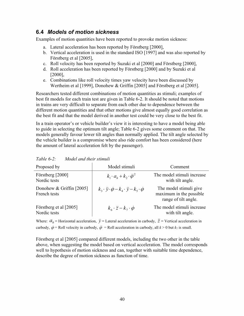
40

6.4 Models of motion sickness Examples of motion quantities have been reported to provoke motion sickness:

a. Lateral acceleration has been reported by Förstberg [2000], b. Vertical acceleration is used in the standard ISO [1997] and was also reported by

Förstberg et al [2005], c. Roll velocity has been reported by Suzuki et al [2000] and Förstberg [2000], d. Roll acceleration has been reported by Förstberg [2000] and by Suzuki et al

[2000], e. Combinations like roll velocity times yaw velocity have been discussed by

Wertheim et al [1999], Donohew & Griffin [2005] and Förstberg et al [2005].

Researchers tested different combinations of motion quantities as stimuli; examples of best fit models for each train test are given in Table 6-2. It should be noted that motions in trains are very difficult to separate from each other due to dependence between the different motion quantities and that other motions give almost equally good correlation as the best fit and that the model derived in another test could be very close to the best fit.

In a train operator’s or vehicle builder’s view it is interesting to have a model being able to guide in selecting the optimum tilt angle; Table 6-2 gives some comment on that. The models generally favour lower tilt angles than normally applied. The tilt angle selected by the vehicle builder is a compromise where also ride comfort has been considered (here the amount of lateral acceleration felt by the passenger).

Table 6-2: Model and their stimuli

Proposed by Model stimuli Comment

Förstberg [2000] Nordic tests

221 ϕ&&⋅+⋅ kak h The model stimuli increase

with tilt angle.

Donohew & Griffin [2005] French tests

ϕϕ &&&&&& ⋅−⋅−⋅⋅ 543 kykyk The model stimuli give maximum in the possible

range of tilt angle.

Förstberg et al [2005] Nordic tests

ϕ&&& ⋅−⋅ 76 kzk The model stimuli increase with tilt angle.

Where: ha = Horizontal acceleration, y&& = Lateral acceleration in carbody, z&& = Vertical acceleration in carbody, ϕ& = Roll velocity in carbody, ϕ&& = Roll acceleration in carbody, all k > 0 but k7 is small. Förstberg et al [2005] compared different models, including the two other in the table above, when suggesting the model based on vertical acceleration. The model corresponds well to hypothesis of motion sickness and can, together with suitable time dependence, describe the degree of motion sickness as function of time.

41

6.5 Time dependence of motion sickness To quantify the time dependence of motion sickness is very interesting for tilting trains, when quantification would become a tool that could be used to minimize motion sickness in an application. The two interesting dependence of time are the Motion Sickness Dose Value (MSDV) and the Net Dose (ND).

The MSDV dependence of time is standardized and indicates the vomiting frequency in percent, ISO [1997].

( )∫ ⋅⋅=τ

0

2)( dttaktMSDV wfMSDVz [6-1]

where )(tawf is the frequency-weighted, Figure 6-2, vertical acceleration [m/s2] and

31=MSDVk [s1,5/m] for a mixed population of male and female adults. Griffin [1990] has

based on the )(tMSDV z derived the illness rating ( )tIR as:

( ) ( )50

tMSDVtIR Z= [6-2]

where ( )tIR is applied on a scale from 0 (feel all right) to 3 (feel dreadful).

Motion sickness dose value can be used with other descriptions of motion than the weighted vertical acceleration, but will always give a value increasing with time.

The ND(t) was derived by Kufver and Förstberg [1999] with the aim to quantify motion sickness as function of time including the recovery.

( ) ( ) ττ τ deACtND tCt

AL ⋅⋅⋅= −⋅−∫

0

)( [6-3]

where )(τA describes the motion, AC and LC are constants.

ND(t) can be used with any description of motion, but rms.-values are mostly used.

ND(t) has the time dependence as one important factor. Förstberg [2000] reports 12 minutes as time constant, a value taken from the recovery after being motion sick. Förstberg et al [2005] reports time constants in the same range, but indicates that value varies at lot. The variation could be depending on the sensitivity threshold that Förstberg [2000] report. This threshold corrupts the time constant at fall ill, this was also the reason why Förstberg used the recovery only when he calculated the time constant. Förstberg et al [2005] has reported time constants taken from various cases. There is also indications on that the time constant is depending on the degree of motion sickness, Golding et al [1995] report time constants in the range of 3 to 5 minutes for low degree of motion sickness.

42

The principal difference between MSDVZ(t) and ND(t) can be seen in Figure 6-4, where ND(t) declines after the motion stops when the MSDVZ(t) keeps its value.

0

1

0 0,5 1 1,5 2 2,5 3 3,5 4

Time

Val

ue

motionMSDVND

Figure 6-4: Principal difference between MSDVZ(t) and ND(t)

6.6 Calculation of net doses based on ideal track geometry The important quantities for motion sickness have all large low-frequency content. The low-frequency importance is further emphasised by band-pass filtering with low-pass frequencies. The low frequencies in the motion quantities come to a large extent from the ideal track geometry. It is therefore natural that Kufver [2005] indicates that it is possible to estimate the motion sickness with quasi-static calculations based on the ideal track geometry. Kufver has validated the motions derived by the quasi-static calculations with simulations on full dynamic models. This procedure is named the simplified method.

The simplified method is aimed at giving planners and engineers a tool for quick and easy analysis of alignment, cant, tilt-compensation ratios and enhanced permissible speed. The analysis neglects influence of track irregularities and vehicle dynamics. However it takes nominal track geometry, train speed, quasi-static sway of the vehicle body (due to primary and secondary suspension deflections) and the basic characteristics of the tilt system into account.

The procedure can be divided in three parts:

1. Calculate the leakage over the track segment (straight track, circular curve or transition curve) based on the net dose received at previous track segment,

2. Calculate the quasi-static movements needed as stimuli input, 3. Calculate the motion dose D based on the quasi-static movements derived in 2

over the track segment and add this dose to 1.

Mathematically this procedure can be expressed as:

)1()1()()1( )/( ++−⋅=+ − kDekNDkND t τ [6-4]

It is basically possibly to use any kind of model for motion sickness stimuli in the simplified method, but there are some limitations that should be considered:

1. The properties describing the stimuli must be constant and non-zero over the circular curve or the transition curve.

2. Frequency weighting can not be applied.

43

6.7 How can motion quantities be limited? The question can be divided in two parts depending on what motion quantities are to be limited. The motion quantities with constant value in circular curves are possible to change by the amount of tilt applied in the train, Figure 6-5. The figure clearly shows that, for a given train speed, all motion quantities can not be reduced at the same time, Kufver [2005].

0

100

200

300

400

0 5 10 15 20

Roll angle [degrees]

Mot

ions

[%]

Pitch velocity

Vertical acceleration -g

Yaw velocity

Lateral acceleration

Figure 6-5: Motion quantities in circular curves as function of applied roll angle for a vehicle running at 20 % enhanced speed, the motions quantities are relative to a non-

tilted vehicle running at 150 mm cant and 150 mm cant deficiency, Kufver [2005].

The motion quantities in transition curves can be reduced by reducing the corresponding (integrated) quantity in the circular curve, i.e. the lateral jerk can be reduced by reducing the lateral acceleration in the circular curve, Table 6-1. The motion quantities in transition curves can also be reduced by extending the transition curve.

6.8 Summary Evidence of motion sickness in both non-tilting and tilting trains have been and is still being reported. The sensory conflict is the most common explanation of motion sickness. Benson [1988] found that the information from sensors in conflict with what is expected by the central nervous system is very provocative.

Förstberg et al [2005] compared different models, when suggesting the model based on vertical acceleration. The model corresponds well to hypothesis of motion sickness and can, together with suitable time dependence, describe the degree of motion sickness as function of time. The model is contradictory to earlier research which showed an optimum tilt angle different from zero.

Quantifying motion sickness is interesting, and two models have been developed. The Motion Sickness Dose Value and the Net Dose Model can both be used with any kind of motion input. The Net Dose Model can describe the recovery after being ill. The motion sickness level can be estimated based on ideal track data input.

45

7 Winter properties Winter problems are found in many different areas, like interior climate, braking, compressed air, doors etc. Winter properties in this study are limited to those connected to tilt and/or high speed. AEIF [2002b] gives some guidance for winter service:

- The rolling stock as well as the on-board equipment, shall be able to put into service and operate normally in the conditions specified in EN 50125-1 standard and function in climatic zones for which the equipment is designed and in which it is likely to run. The different environmental conditions likely to be experienced on the lines worked are specified in the infrastructure register.

Winter problems connected to tilt and/or high speed can be divided in two groups.

1. Lift of ballast stones 2. Snow packing

7.1 Lift of ballast stones

7.1.1 The phenomenon Lifting ballast stones have a strong relation to safety. A ballast stone is approximately 0,05m in diameter and can have the same speed (or even higher) as the train. At speeds above 300 km/h the stone may be lifted by the drag from the passing train. Jänsch [1987] mentions that stone lift has been observed at as low speed as 220 km/h at summer conditions. At lower speeds something must hit the stone in order to lift; normally because ice is dropping from the train. Once a stone has lifted the lifted stone can hit other stones that also may lift. Ballast stone lift may in this sense be seen as a winter phenomenon. The stone lift phenomenon is described by Shinojima [1984] and Felsing [1982]. In Sweden this problem raised with the introduction of X2000 which run at higher speed than other trains at that time, which run at 130 -160 km/h and did not receive much of a problem. The carbody tilt on the X2000 may had contributed to the stone lift indirectly when the risk of dropping ice may be higher on a tilting bogie with more moving parts than for a non-tilting bogie. The conclusion must still be that the speed is important.

7.1.2 Countermeasures to lift of ballast stones The countermeasures to stone lift may be divided in four groups:

1. Restricting the snow to build up on the train, refer to Section 7.2 2. Restricting the ballast from being hit by ice 3. Restricting the stones from lifting 4. Others

Group 2, restricting the ballast from being hit by ice Felsing [1982] had found that falling ice breaks in pieces when it hits the track and that no stone is lifted if the ice hits a sleeper first. Lowering the ballast level between the rails became the solution that insured that the ice hits a sleeper first. This solution is used in

46

Germany, Japan as well as in Sweden. One option to lowering the ballast is to increase the height of the sleeper, either by manufacturing them high or to mount an additional device on them afterwards.

Group 3, restricting the stones from lifting Shinojima [1984] show two possible solutions restricting the ballast stones from lifting.

• Using a net with holes smaller than the stone which is attached to the rails or sleepers

• Using rubber carpets made from used car tires. The latter is applied in snowy regions at the Japanese Shinkansen lines, particularly close to stations where the impact of a lifted stone can be large, Figure 7-1.

Figure 7-1: Rubber carpets used in Japan at Shinkansen lines (JR-East),

photo by Rickard Persson

Group 4, others This group contains countermeasures that do not fit any of the three other groups.

• Shinojima [1984] describes how snow is melted by water sprinklers to avoid that snow gather on the track.

• The track could also be covered by snow shelters (tunnels), a method applied both in Japan and in Norway.

• Jänsch [1987] give temporary speed restrictions to 160 km/h as a solution.

Some of the countermeasures suggested do extinguish the problem, others reduce the problem and actions must still be taken to insure that the train is not damaged by a stone hit. Areas where protection may be considered are axles, brake units, hoses and cables.

Increased speed in Sweden from 200 km/h as today to 250 km/h or more will increase the energy in the ice falling down and thereby increasing the risk of stone lift. The risk with lifted stones should be considered when selecting countermeasures. At sections with high risk, like station areas, countermeasures that extinguish the problem should be considered.

47

7.2 Snow packing

7.2.1 The phenomenon Snow packing occurs on all trains running under winter conditions; still the phenomenon has a relation to both high speed and tilt. Packed snow will under pressure and/or heat transform to ice. Dropped ice may be the start of ballast stone lift as mentioned in Section §7.1. Packed snow may also restrict movements of moving parts like brake equipment, suspensions, doors, moving foot steps and tilt. This study will concentrate on the tilt movement as the other equipment is not different from non-tilting trains.

The impact from packed snow can be divided in three categories: 1. Impact on track forces 2. Impact on passenger comfort 3. Impact on equipment

Impact on track forces A typical tilt actuator has a force capacity in the range of 60 to 100 kN, that is in the same range as the track forces. Tilt forces transferred to track forces may result in safety-related issues. This issue is evident also without snow packing for tilt systems with one control loop for each bogie. Packed snow will make it evident for all types of active tilt systems. Snow packed between bogie and carbody will restrict the tilt movement. There will be twist forces through the carbody if the movement possibility between bogies differs. Twist forces will result in diagonal wheel unloading which may be safety critical. The risk of diagonal wheel unloading must be mitigated. Normal means of mitigation are force-protective devices and supervision of force and/or tilt angle.

Impact on passenger comfort Snow packed between bogie and carbody is a general winter problem, but it is much more likely on tilting vehicles as the tilt movements contribute to the packing of the snow. The packed snow restricts the normal movement over the secondary suspension and deteriorates the passenger comfort. Packed snow can also restrict the tilt movement as such which will result in larger lateral acceleration in the carbody and deteriorated passenger comfort.

Impact on equipment Protecting equipment from snow, ice and humidity is standard measures for trains used under winter conditions. The tilt adds further conditions to consider as result of its large movements. Typical problems are: cables and hoses that get caught by ice and then torn off by tilt movement, forces from tilt moving packed snow that presses and damages equipment.

7.2.2 Countermeasures to snow packing Countermeasures to snow packing can be divided in two groups, Table 7-1.

48

Table 7-1: Countermeasures to snow packing Restrict the snow from building up Arrange the snow to fall of

1. Fill the volume with something else 2. Limit horizontal surfaces 3. Aerodynamic design 4. Enclose the volume 5. Heat

1. Low adhesion surfaces 2. Flexible surfaces 3. Heat

The best solution differs from case to case and combination may give even better result. Shinkansen train passes some areas of Japan that have a lot of snow. The most modern Shinkansen trains combine all five measures to restrict snow from building up.

1. Fill the volume with something else Most of the equipment have been moved down in the underframe, the open volume for the bogie is limited

2. Limit horizontal surfaces The bogie frame is a slender design avoiding unnecessary horizontal surfaces facing up

3. Aerodynamic design No comments necessary

4. Enclose the volume The underframe is enclosed and the bogie volume is covered by bogie skirts.

5. Heat Many bogies are driven and the energy loss can be used to keep the bogie volume warm enough not to pack snow.

7.3 Summary Winter problems connected to tilt and/or high speed can be divided in ballast stone lift and snow packing.

At speeds above 300 km/h the stones may be lifted by the drag from the passing train, at lower speeds something must hit the stone in order to lift; normally because ice is dropping from the train. The countermeasures to ballast stone lift may be divided in restricting the snow to build up, restricting the ballast from being hit by ice and restricting the stone from being lifted.

The risk with lifted stones should be considered when selecting countermeasures. At sections with high risk, like station areas or in close neighbourhood to humans, countermeasures that extinguish the problem should be considered.

Snow packing occurs on all trains running under winter conditions; still the phenomenon has a relation to both high speed and tilt. Tilt forces transferred to track forces may result in safety-related issues. Snow packed between bogie and carbody will restrict the tilt movement. There will be twist forces through the carbody if the movement possibility between bogies differs. Twist forces will result in diagonal wheel unloading which may be safety critical. The risk of diagonal wheel unloading must be mitigated. Normal means of mitigation are force-protective devices and supervision of force and/or tilt angle.

49

Part 2, Analysis

51

8 Analysis of vehicle and infrastructure

8.1 Vehicles

8.1.1 Availability of tilting trains Gustavsson [2003] considers the availability of tilting trains being able to run 250 km/h and come to the conclusion that the availability will be limited as the present interest for such trains is small. Table 8-1 gives examples of recently built tilting trains with top speed of 200 km/h or above. Only one of the trains in Table 8-1 run at 250 km/h, but all these suppliers produce non-tilting trains for 250 km/h or above. The conclusion must be that tilting trains being able to run 250 km/h will be available on request. Table 8-1: Examples of tilting trains with top speed of 200 km/h or above

Train Top speed Supplier Comment

ETR600 (the new Pendolino)

250 km/h 1) Alstom Deliveries ongoing. Some updates compared with older

versions

Pendolino Britannica 200 km/h Alstom Electro-mechanical actuators

ICE-T 230 km/h Siemens Deliveries ongoing

Acela 240 km/h Bombardier

Signatur 210 km/h Bombardier 1) Cant deficiency for tilting trains is not used on high-speed lines in Italy, Casini [2005].

8.1.2 Tilt actuator Different suppliers of tilting trains come to different conclusions on what actuator to use. A Japanese study made by Enomoto et al [2005] come to the conclusion that electro-hydraulic actuators are the best choice. This study was made for natural tilted trains were the actuator was used to improve performance. Here a similar study is made for an actively tilted train.

The state of the art actuator for active tilt is the electro-mechanical actuator, which have advantages but also disadvantages. Table 8-2 compares different actuators with reference to the hydraulic (split) system.

52

Table 8-2: Actuator comparison for actively tilted trains

Property Pneumatic Hydraulic El-mechanical El-hydraulic

Response Worse Reference Equal Equal

Safety Worse Reference Worse 1, 2) Worse 2)

Mass Equal Reference Better Better

Size Equal Reference Better Better

Cost Better Reference Worse 3) Worse 3)

Maintenance Better Reference Better Better 1) The actuator may jam which may lead to diagonal wheel unloading if appropriate actions

are not taken 2) The hydraulic split system may have only one control loop, which insures the same forces

in the two bogies. 3) The hydraulic split system may be built by standard components produced in large series.

It is difficult to pick a winner out of Table 8-2, the hydraulic split system have its advantages on safety and cost, where the electro-mechanical and electro-hydraulic systems have their advantages on mass, size and maintenance. The underframe space for tilt equipment on multiple units is very limited; this may force the supplier to prioritize size. The electro-hydraulic actuator may be the best choice for these trains as it is easier to handle the safely-related issues with electro-hydraulic actuators than with electro-mechanical actuators. Not considered here is the customer preference, which could be important.

8.2 Infrastructure

8.2.1 Speed limitations The speed for tilting trains in Sweden is given by 30 % enhanced speed compared with the speed for category A trains (due to properties in the signalling system) and 245 mm cant deficiency, whichever giving the most restrictive speed. Kufver [2005] has stated that 30 % enhanced speed compared with the speed for category A trains may result in that 245 mm cant deficiency can not be utilized in some curves. This is true but it is more common that 30 % enhanced speed can not be utilized. 30 % enhanced speed compared with category A trains corresponds to a cant deficiency of 273 mm assumed that the category A trains utilize 100 mm cant deficiency and that the installed cant is 150 mm. 245 mm of cant deficiency corresponds under the same conditions to 25 % enhanced speed compared with category A trains. The actual utilization of cant deficiency is depending on limitations in the signalling system that only allows speed in steps of five km/h. This effect comes in twice for vehicles running at enhanced speed, once when the base speed is set and once when the enhanced speed is set. The utilized cant deficiency can therefore be considerably lower than the allowed cant deficiency. The range of utilized cant deficiency is shown in Figure 8-1, which is based on curve radius from 300 meters and up. The maximum utilized cant deficiency is equal to the allowed.

53

0

50

100

150

200

250

300

350

0 5 10 15 20 25 30 35 40

Enhanced speed [%]

Can

t def

icie

ncy

[mm

]

Maximum utilized cant deficiency =maximum allowed cant deficiency

Figure 8-1: Range of utilized cant deficiency as function of enhanced speed

Relating the speed for tilting trains to the speed for non-tilting train results in:

• that the maximum cant deficiency can not be utilized in case that the calculated enhanced speed is lower than the speed allowed from a cant deficiency point of view,

• that special speed restrictions must be made when the calculated enhanced speed is higher than the speed allowed from cant deficiency point of view.

The speed for tilting trains should be based on cant deficiency allowed for tilting trains rather than 30% enhanced speed compared with the speed for category A trains. The new signalling system for Europe (ERTMS) will make this possible.

8.2.2 Choice of cant The choice between cant and cant deficiency does not have a simple answer. The track standards often give rather wide range of possible combinations. The choice get even more complex when different train categories must be considered. Following choices can be made for a curve with an equilibrium cant of 220 mm for category A:

1. Install 150 mm cant which currently is the maximum allowed cant in Sweden 2. Install 120 mm cant which gives 100 mm cant deficiency for category A. 3. Install something between 1 and 2.

In the same curve as above there will also run trains of category B at 10 % enhanced speed and trains in category S at 30 % enhanced speed. The three choices are then modified to:

1. Install 150 mm cant which currently is the maximum allowed cant in Sweden 2. Install 130 mm cant which gives 245 mm cant deficiency for category S. 3. Install something between 1 and 2.

54

The limitations on cants to install as function of equilibrium cant for trains in category A are shown in Figure 8-2.

0

20

40

60

80

100

120

140

160

0 50 100 150 200 250 300

Equilibrium cant for trains in category A [mm]

Can

t [m

m]

Maximum allowed cant = 150 mm

Cant deficiency for category A = 100 mm

Cant deficiency for category S = 245 mm

Cant deficiency for category A = 0 mm

Cant deficiency for category B = 150 mm

Figure 8-2: Possible cant as function of equilibrium cant for trains of category A

There are some more relations to consider:

• The relation between the numbers of train per day in each category, • The shortest transition curve can be derived from the requirements on rate of

change of cant and rate of change of cant deficiency, • The passenger comfort has a strong relation to cant deficiency. Cant deficiency

above a certain level leads to discomfort, • Motion sickness has a relation to roll. Minimizing roll will limit the risk for

motion sickness in tilting trains, which can be achieved by minimizing the cant, • Carbody tilt uses cant information to improve performance, • Cant excess for slow trains (freight).

With all limitations on cant considered there still remains a wide range, it might be proper to suggest some guidelines for selection of cant on lines with all categories of trains. The guidelines are given as function of equilibrium cant for category A trains. The tilting trains are here assumed to apply a fixed ratio between cant deficiencies and tilt angles. Kufver & Persson [2006] has shown how variable ratio between cant deficiencies and tilt angles can be used to optimize comfort and limit risk of motion sickness. The guideline derived here is a balance between comfort according to the PCT criterion and the risk for motion sickness as function of roll motions. The PCT criterion consists of two parts, see Section 5.3.1 for details, (constants for seated passengers used):

the lateral part: [ ] 0);0,0590,09680,0897(max%100max1max1 −⋅+⋅⋅ ss yy &&&&& and

the roll part: 1,626max1 )0,916(%100 sϕ&⋅⋅

The result of these guidelines is shown in Figure 8-3.

55

Low equilibrium cant (0 – 49 mm) The low equilibrium cant results in a low lateral acceleration which will make the lateral part of the CTP criterion zero for all train categories. The cant may be set to 0 to minimize the roll part.

Medium equilibrium cant (50 – 149 mm) Cant different from 0 is needed to make the lateral part of the CTP criterion zero for category B. Carbody tilt is used to reduce the lateral acceleration for category S. The cant should be large enough to improve tilt performance, here assumed as 30 mm. The cant is set to maximum of equilibrium cant minus 50 mm and 30 mm.

High equilibrium cant (150 – 234 mm) Considerations to motion sickness in tilting trains should be taken. The lateral part of the

CTP criterion will not be zero for category B. The cant is set to 60 % of equilibrium cant for category A + 10 mm.

Very high equilibrium cant (235 - 250 mm) Maximum cant must be installed to meet requirements on cant deficiency. Large roll motions may contribute to motion sickness in tilting trains.

0

20

40

60

80

100

120

140

160

0 50 100 150 200 250 300Equilibrium cant for trains of category A [mm]

Can

t [m

m]

Low Medium High Very high

Maximum MinimumGuideline

Figure 8-3: Cant as derived from the guidelines as function of equilibrium for trains of

category A

56

Figure 8-4 shows the installed cant on the Stockholm – Gothenburg line as function of equilibrium cant for category A trains at today’s speeds. Some curves have installed cant outside the possible area indicating that at least one train category not has been considered or that there are more to consider than in the scope of this study.

0

20

40

60

80

100

120

140

160

0 50 100 150 200 250 300Equilibrium cant for trains of category A [mm]

Can

t [m

m]

Figure 8-4: Installed cant Stockholm – Gothenburg as function of equilibrium for

trains of category A

8.3 Summary The major train suppliers have recently built tilting trains for above 200 km/h and it is likely that tilting trains for 250 km/h will be available on request.

Speed limitations for tilting trains in Sweden are set as function of the speed for trains in category A. The performance of tilting trains will be better utilized is the speed is directly set based on cant deficiency. The new signalling system ERTMS for Europe will make this possible.

Guidelines for installation of cant are given optimizing the counteracting requirements on comfort in non-tilting trains and risk of motion sickness in tilting trains. The guideline is finally compared with the installed cant on the Stockholm – Gothenburg line.

57

9 Analysis of services suitable for tilting trains Tilting trains are more or less suitable for different services. This chapter gives different views on suitability.

Simulations of running times given in this chapter are received at 3% lower speeds than allowed from the equilibrium cant and maximum speed points of view. This is made in order to achieve a running time margin due to non-optimum performance of the train driver, further running time margins and dwelling times must be added to receive running times suitable for time tables.

Assumptions for the calculations: • Enhanced speed is allowed at the same track sections as today, • The maximum speed is set depending on the equilibrium cant, i.e. the cants and

length of transitions of today may be changed where needed, • Maximum allowed cant excess for freight trains is 110 mm at 90 km/h, • Maximum allowed cant deficiency is 300 mm up to 225 km/h and above that

reduced with 1 mm per 1 km/h due to cross-wind effects.

9.1 Running time – cant deficiency, top speed or tractive performance

Running times are dependent on many factors. Cant deficiency, top speed and tractive performance are key factors which are like a chair with their legs, where a change on one leg must go together with changes on the other legs to make a good chair, see Figure 9-1.

Top speed

Cant deficiency Tractive performance

Top speed

Cant deficiency Tractive performance Figure 9-1: Cant deficiency, top speed and tractive performance

9.2 Performance of X2000 One example on the relation between cant deficiency, top speed and tractive performance comes from the time when these factors where established for the Swedish tilting train X2000, see Table 9-1.

58

Table 9-1: Key performance factors, X2000 Performance factor Value Number of vehicles 6 1) Cant deficiency 245 mm Weight with seated passengers 339 ton Top speed in service 200 km/h Short-term power 3,9 MW Tractive effort at start 160 kN Braking rate in simulations 0,6 m/s2 Running resistance 25.7402000 vvR ⋅+⋅+= [N]

where v is speed [m/s] 1) The data is given for the original formation with one loco and 5 trailer vehicles, today most

trains run with 6 trailer vehicles.

The X2000 train was optimized for the line Stockholm – Gothenburg, the curve distribution for this line is shown in Figure 9-2. Simulation of the running time for the original key performance factors and with improved key performance factors show how well the train was optimized for the service.

The original setup with 4 intermediate stops has a running time of 2:46 excluding stopping times and margins. The effect on running time by change of one or more of the key performance factors with approximately 25 % is shown in Table 9-2. Table 9-2: Effect on running time on the Stockholm – Gothenburg line

Changed key performance factor Cant deficiency Top speed Short-term power

Running time effect

300 mm - 4 minutes 250 km/h - 5 minutes 1) 4,8 MW - 1 minute

300 mm 250 km/h - 12 minutes 300 mm 4,8 MW - 4 minutes

250 km/h 4,8 MW - 7 minutes 300 mm 250 km/h 4,8 MW - 13 minutes

1) 4 minutes reduced running time is received at a top speed of 220 km/h.

Following conclusions may be drawn: • No single factor can give more than 5 minutes improvement on the 3 hour journey, • Combination of two or more factors is needed to receive 10 minutes of

improvement, • Combinations of factors give more improvement than the sum of the individual

factors.

59

9.3 Performance of a new tilting train

9.3.1 The tracks The Stockholm – Gothenburg relation is suitable as an example also here, as this is one of the most important services in Sweden, but tilting trains might be useful on other types of relations as well; the Gothenburg – Kalmar line is used as an example with quite different conditions. The tracks may be characterized by the curve distribution which may be given as percentage of the total length of the track. The curve radius indicated is the mean radius in that group, i.e. the curves in group 1000 meter range from 900 to 1100 meters.

The Stockholm – Gothenburg line This line has a variety of curves ranging from 352 m radius and up. The curve distribution for the line Stockholm – Gothenburg is shown in Figure 9-2. The length of the circular curves (transition curves are excluded) with radii less than 6000 meter constitutes in total 19 % of the line. The total length of this line is 457 km.

0

1

2

3

4

5

250

400

600

800

1000

1200

1400

1600

1800

2000

2200

2400

2600

2800

3000

3500

5000

Curve radius [m]

Cur

ve le

ngth

[%]

Figure 9-2: Distribution of circular curves with radii less than 6000 meter as function

of the total length of the line Stockholm – Gothenburg

The Gothenburg – Kalmar line This line has a variety of curves ranging from 206 m radius and up. The curve distribution for the line Gothenburg – Kalmar is shown in Figure 9-3. The length of the circular curves with radii less than 6000 meter constitutes in total 21 % of the line. The total length of this line is 352 km.

60

0

1

2

3

4

5

250

400

600

800

1000

1200

1400

1600

1800

2000

2200

2400

2600

2800

3000

3500

5000

Curve radius [m]

Cur

ve le

ngth

[%]

Figure 9-3: Distribution of circular curves with radii less than 6000 meter as function

of the total length of the line Gothenburg – Kalmar

9.3.2 The trains The base for the running times is a future train with key performance factors as shown in Table 9-3. The tilting and the non-tilting train only differ on the allowed cant deficiency.

Table 9-3: Key performance factors, future train Performance factor Value Number of vehicles 6 Cant deficiency 1) 150 - 300 mm Weight with seated passengers 360 ton Top speed in service 1) 180 – 280 km/h Short-term power 1) 2,7 – 9,0 MW Starting acceleration 1) 0,6 – 1,0 m/s2 Braking rate in simulations 0,6 m/s2 Running resistance 25,6602400 vvR ⋅+⋅+= [N]

where v is the speed [m/s] 1) This factor is part of the optimisation

9.3.3 Cant deficiency The relation between cant deficiency, top speed and tractive performance is strong as mentioned above, but still it is possible to study them one at a time. The first parameter to be studied is the cant deficiency, or rather the equilibrium cant which is the sum of the cant and cant deficiency. Service with future tilting trains is studied in relation to service with non-tilting vehicles. Four different combinations of cant and cant deficiencies can be distinguished based on the situation today and what could likely be achieved tomorrow i.e. until 2012 - 2014, Table 9-4.

61

Table 9-4: Possible equilibrium cant

Vehicle & Track Cant [mm] Cant deficiency [mm]

Equilibrium cant [mm]

Non-tilt, today 150 150 300

Non-tilt, tomorrow 160 165 325

Tilt, today 150 245 395

Tilt, tomorrow 160 300 460 The result of the running time simulations on Stockholm – Gothenburg can be seen in Figure 9-4, where the running times are given as function of equilibrium cant. The stopping pattern includes 8 intermediate stops, but this has a quite limited impact on the difference between the different combinations. The four graphs represent four vehicles with low and high top speed and low and high tractive power. The running times improves with increased equilibrium cant independently of maximum speed and tractive power.

02:30

02:35

02:40

02:45

02:50

02:55

03:00

03:05

280 300 320 340 360 380 400 420 440 460 480

Equilibrium cant [mm]

Run

ning

tim

e [h

]

200 km/h, 3,6 MW

280 km/h, 3,6 MW

200 km/h, 9,0 MW

280 km/h, 9,0 MW

X2000

Figure 9-4: Simulated running times Stockholm – Gothenburg as function of

equilibrium cant, with 8 intermediate stops The result of the running time simulations on Gothenburg – Kalmar can be seen in Figure 9-5, where the running times are given as function of equilibrium cant. The stopping pattern includes 11 intermediate stops, but this has a quite limited impact on the difference between the different combinations. The four graphs represent four vehicles with low and high top speed and low and high tractive power. The running times improves with increased equilibrium cant independently of maximum speed and tractive power.

62

02:35

02:40

02:45

02:50

02:55

03:00

03:05

03:10

280 300 320 340 360 380 400 420 440 460 480Equilibrium cant [mm]

Run

ning

tim

e [h

]

180 km/h, 3,6 MW

180 km/h, 9,0 MW

250 km/h, 3,6 MW

250 km/h, 9,0 MW

Figure 9-5: Simulated running times on Gothenburg – Kalmar

as function of equilibrium cant, with 11 intermediate stops

Conclusion on cant deficiency The study on the influence of cant deficiency, or rather equilibrium cant, shows that running times improves with increased equilibrium cant independently of maximum speed and tractive power for the two studied lines.

One interesting conclusion is that a non-tilting vehicle will, independent of top speed and tractive power, have longer running times than a tilting train with today’s maximum speed and tractive power on both lines studied.

9.3.4 Top speed In the previous section it becomes clear that high equilibrium cant is beneficial for the running time. If an equilibrium cant of 460 mm is selected, the relation between top speed and running time can be studied. The studied top speeds range from 180 km/h to 280 km/h.

The Stockholm – Gothenburg line The result is displayed in Figure 9-6. A top speed of 240 - 250 km/h seams to be close to an optimum from the running time point of view only. Higher top speed can not significantly improve the running time even if high tractive power is selected. The stopping pattern includes 8 intermediate stops.

63

02:30

02:35

02:40

02:45

02:50

190 200 210 220 230 240 250 260 270 280 290Top speed [km/h]

Run

ning

tim

e [h

:m]

3,6 MW

5,4 MW

7,2 MW9,0 MW

Figure 9-6: Simulated running times Stockholm – Gothenburg as function of top speed,

at 460 mm equilibrium cant and with 8 intermediate stops

The Gothenburg – Kalmar line The result is displayed in Figure 9-7. A top speed of 200 km/h seams to be close to an optimum from the running time point of view only. Higher top speed can not significantly improve the running time even if high tractive power is selected. The stopping pattern includes 11 intermediate stops.

02:30

02:35

02:40

02:45

02:50

170 180 190 200 210 220 230 240 250 260Top speed [km/h]

Run

ning

tim

e [h

:m] 3,6 MW

5,4 MW7,2 MW9,0 MW

Figure 9-7: Simulated running times Gothenburg – Kalmar as function of top speed,

at 460 mm equilibrium cant and with 11 intermediate stops

64

Conclusion on maximum speed The study of maximum speed shows that running times improves with increased maximum speed. However, the benefit of increased maximum speed is small above a certain level. The conclusion is independent of tractive power for the two studied lines.

9.3.5 Tractive power In the previous section it becomes clear that increased maximum speed is, up to a certain level, beneficial for the running time. This level is about 250 km/h at the Stockholm – Gothenburg line and 200 km/h at the Gothenburg – Kalmar line. If an equilibrium cant of 460 mm, according to CEN [2005] is selected, the relation between tractive power and running time can be studied. The studied tractive power ranges from 2,7 MW to 9,0 MW. The base for the running times is here a future tilting train with key performance factors as shown in Table 9-4.

The Stockholm – Gothenburg line The result is displayed in Figure 9-8. Tractive power of 4 – 6 MW seams to be close to an optimum, the optimum is to some degree depending on the number of stops, more stops requires more power. The effect of increased starting acceleration is shown for the case with 4 stops, a starting acceleration of 1,0 m/s2 is compared with the otherwise used 0,6 m/s2.

02:20

02:25

02:30

02:35

02:40

02:45

02:50

0 2 4 6 8 10Tractive power [MW]

Run

ning

tim

e [h

:m]

8 stops, 0,6 m/s2

4 stops, 0,6 m/s2

4 stops, 1,0 m/s2

0 stops, 0,6 m/s2

Figure 9-8: Simulated running times Stockholm – Gothenburg as function of tractive

power, at 460 mm equilibrium cant and 250 km/h top speed

The Gothenburg – Kalmar line The result is displayed in Figure 9-9. Tractive power of 4 – 6 MW seams to be close to an optimum, the optimum is to some degree depending on the number of stops, more stops requires more power. The effect of increased starting acceleration is shown for the case with 6 stops, a starting acceleration of 1,0 m/s2 is compared with the otherwise used 0,6 m/s2.

65

02:20

02:25

02:30

02:35

02:40

02:45

02:50

0 2 4 6 8 10Tractive power [MW]

Run

ning

tim

e [h

:m]

11 stops, 0,6 m/s2

6 stops, 0,6 m/s2

6 stops, 1,0 m/s2

0 stops, 0,6 m/s2

Figure 9-9: Simulated running times Gothenburg – Kalmar as function of tractive

power, at 460 mm equilibrium cant and 250 km/h top speed

Conclusion on tractive power The study of tractive power shows that running times improves with increased tractive power; however the benefit of increased tractive power is small above a certain level. Increased starting acceleration is mainly effective at start, the benefit is therefore larger the more stops and starts there are. The conclusion is independent of line studied.

9.4 Distance between stops The two studied lines in Section 9.3 show the advantage of tilting trains; both are examples of services with long or intermediate distances between stops. On the other hand we have services with short distances between stops, where tractive power may be more beneficial than tilt. It is interesting to study tilting capability versus tractive power for services between these two extremes. This study is limited to running times, other important aspects are energy consumption and maintenance costs (in particular brake pads).

Two hypothetical lines are used here; they have stations with equal distances and curves with 600 meter and 1000 meter radius respectively. 325 mm equilibrium cant is used for the non-tilted train and 460 mm for the tilted train. The resulting speed limitations are shown in Table 9-5, and they are assumed to be valid for the whole hypothetical line. Table 9-5: Speed limitations

Equilibrium cant R = 600 m R = 1000 m

325 mm 125 km/h 165 km/h

460 mm 150 km/h 195 km/h

66

The line speeds are combined with key performance factors given in Table 9-6.

Table 9-6: Key performance factors Performance factor Value Number of vehicles 6 Weight with seated passengers (dynamic weight)

360 (380) ton

Short-term power 1) 2,7 – 9,0 MW Starting acceleration 1) 0,6 – 1,0 m/s2 Braking rate in simulations 0,6 m/s2 Running resistance 25.6602400 vvR ⋅+⋅+= [N]

where v is the speed [m/s] 1) This factor is part of the optimisation

This comparison is made by calculating the average speed for different tractive performances combined with the speed limitations in Table 9-5. The result is shown in Figure 9-10 as the difference in average speed between a non-tilted vehicle with 2,7 MW tractive power and 0,6 m/s2 starting acceleration, i.e. a low tractive performance and:

1. A non-tilted vehicle with 9,0 MW tractive power and 1,0 m/s2 starting acceleration, i.e. a high tractive performance

2. A tilted vehicle with 2,7 MW tractive power and 0,6 m/s2 starting acceleration, i.e. a low tractive performance

The break point is found at 6 km between stations for the line with 600 m curve radius, shorter distances give benefit for higher tractive performance, longer distances benefit for tilt. The break point is found at 20 km between stations for the line with 1000 m curve radius.

0

2

4

6

8

10

12

14

16

18

20

2 4 6 8 10 20 40Distance between stops [km]

Aver

age

spee

d im

prov

emen

t [km

/h]

R=600m, tilt, low tractive perf.R=1000m, tilt, low tractive perf.

R=600m, no tilt, high tractive perf.

R=1000m, no tilt, high tractive perf.

Figure 9-10: Simulated average speed as function of distance between stops

67

9.5 New tracks, for tilting or high-speed trains?

9.5.1 Background Building new tracks is an investment in infrastructure that will be used for a long time. Today BV applies the S250 standard, which means that a train with carbody tilt shall be able run at 250 km/h. The only existing carbody tilting train in Sweden (X2000) has a maximum speed of 200 km/h, presently giving a margin between track and vehicle of 50 km/h. Figure 9-11 shows how long-term trend of the top speed developed in Sweden over the last 150 years.

1840 1890 1940 1990 2040

Year

Top

spee

d

?

130

50

200

[km/h](log)

90

Figure 9-11: Top speed in Sweden during the last 150 years

The relation between travelling time and the market share for trains should also be considered when selecting tracks for the future. This relation is known to be particularly strong at travelling times in the range of three hours for train travel, where longer times give advantages for air services and shorter time advantages for train services, Kristenson [2004].

In the 1980s German high-speed lines where built to allow high-speed trains and freight trains on the same line. This resulted in many bridges and tunnels (46% of the line between Hannover and Wurzburg) and this standard has today been abandoned due to the high investment cost. The investments cost can in general be reduced by avoiding construction of bridges and tunnels. To minimize the length of bridges and tunnels, the alignment must be adopted to the landscape as far as possible. However, high-speed lines require large radii, both vertically and horizontally, making it difficult to avoid bridges and tunnels. Also environmental issues and built-up areas give restrictions on extensive construction work. These facts lead to basically two possibilities for Swedish conditions:

68

S250 This is the applied standard for new lines of today. The horizontal alignment allows non-tilting trains of category B (150 mm cant deficiency) with a top speed of 220 km/h and tilting trains of category S (245 mm cant deficiency) with a top speed of 250 km/h. The horizontal radius recommended by Banverket, but not always kept, allow for some speed upgrade in the future. The S250 may be built to allow freight services (maximum gradient 10‰), but also as dedicated passenger lines.

A300 A high-speed line is the alternative. The horizontal alignment allowing non-tilting trains of category A (100 mm cant deficiency) with a top speed of 280 km/h or more. This is a dedicated passenger line with maximum gradients not restricted to10‰.

The key questions are:

1. Will the capacity be sufficient if with a mixture of train categories operating on the same line?

2. Is there an existing line running in parallel, to be used by slow trains?

The first choices of line as function of the key questions could be as in Table 9-7.

Table 9-7: First choice of line as function of key questions

Will the capacity be sufficient with a mixture of train categories operating

on the same line?

Is there an existing parallel line?

First choice

Yes Yes S250 1)

Yes No S250 2)

No Yes A300 3) 1) Primarily upgraded lines. 2) Freight services assumed, if not A300 might an option 3) The existing line is combined with a dedicated passenger line to meet the requirements on

capacity. The additional costs for A300 compared with S250 can probably be motivated in a cost – benefit – analysis by the high capacity requirement. S250 might be an option if the number of foreseen passenger services is low.

The top speed development and relation between travelling time and market share both indicates that other choices than the S250 standard should be investigated, particularly if an existing line can be used for freight and possibly also for regional services. There may, of cause, also be intermediate alternatives being the optimum choice. For example lines where non-tilting trains may run 250 km/h and tilting trains 300 km/h. However, in the present study the extreme alternatives S250 and A300 are used.

69

9.5.2 Consequences on capacity caused by different train categories For a double track railway, combining different train categories generally lower the line capacity due to the difference in average speed between the different trains, Figure 9-12.

0

10

20

30

40

50

60

0 20 40 60 80 100 120

Time [Minutes]

Dis

tanc

e [k

m]

FT HS FT + HS

Figure 9-12: Line capacity, for Freight trains (FT) only, High-speed trains (HS) only

and combined freight and high-speed trains (FT+HS) A simple study is made here to highlight the relation between the distance between passing possibilities and line capacity. The study is limited to a double track line, one travel direction and with assumptions according to Table 9-8. Table 9-8: Assumptions for capacity study Property Value

Speed of high-speed train 250 km/h

Speed of freight train 100 km/h

Minimum headway time 3 minutes The result is shown in Figure 9-13. The necessary distance between the passing possibilities becomes short when the number of freight trains increases. As an example, running three high-speed trains and three freight trains per hour give the maximum distance between passing possibilities of 39 km. It is assumed that high-speed trains may be run in convoy if the number of high-speed trains is higher than the number of freight trains, Figure 9-14. Running freight trains in convoy may be effective if the number of freight trains is higher than the number of high-speed trains, but this will add side tracks at the passing places. The average speed for the freight trains running three high-speed trains and three freight trains per hour is 80 km/h.

70

The density of passing possibilities as determined here would not be unrealistic. However, this is an estimation made with assumed ideal conditions regarding time precision. If some of the trains are some minutes late practical capacity of the line becomes lower and the necessary distance between passing possibilities decreases. For the quite modest degree of time precision now being practice in Europe (incl. Sweden) the latter case is likely. This will favour shorter distances between passing possibilities.

0

10

20

30

40

50

60

70

80

90

100

1 2 3 4 5 6

Number of freight trains per hour

Dis

tanc

e be

twee

n pa

ssin

g po

ssib

ilitie

s [k

m]

1 or 2 HS

5 or 6 HS 1 to 3 HS

4 to 6 HS

5 or 6 HS

1 to 4 HS1 to 5 HS

6 HS 1 to 6 HS

Figure 9-13: Distance between passing possibilities as function of the number of

freight trains per hour and the number of high-speed trains (HS)

0

10

20

30

40

50

60

70

80

90

100

0 10 20 30 40 50 60 70 0 10 20 30 40 50 60 70 80

Time [Minutes]

Dis

tanc

e [k

m]

Figure 9-14: Graphic visualizing of 3 freight trains per hour combined with 3 high-

speed trains (left) or 6 high-speed trains (right)

71

9.6 Upgrading tracks or tilting trains Tilting trains can in some cases be an alternative to upgrading the lines to larger curve radii. One such an occasion is when a stiff time table is desired and the running times with the existing vehicles exceeds a certain maximum. Dalabanan between Uppsala and Borlänge in Sweden is one example. This is a single track line, where the stations almost come with half-hour time intervals. A stiff time table with train crossings at places with passenger exchange would be possible if the intervals were less than a half hour, Larsson [2004]. Snickarbo is the only station where train crossing must take place without passenger exchange, Figure 9-15. There are two sections on this line where the running time (incl. margins) is somewhat longer than the half hour, Uppsala – Sala and Snickarbo – Borlänge. Introducing tilting trains would here be an option to upgrade the line on these sections. The cost for upgrading the line will here be compared with the difference on cost between non-tilting and tilting trains.

Uppsala C

Sala

Arlanda C

Avesta KrylboSnickarbo

Borlänge

Mora

Stockholm C

Gagnef

Rättvik

0

50

100

150

200

250

300

07:00 07:30 08:00 08:30 09:00 09:30 10:00 10:30 11:00 11:30

[km]

Figure 9-15: Graphic visualizing of one hour service in each direction on Dalabanan

9.6.1 Track upgrading The distance between Uppsala and Sala is approximately 62 km and have one intermediate station, Heby, where the operator want to stop for passenger exchange. The existing time table has 33 minutes running time for non-tilting trains without intermediate stops and 38 minutes with 2 intermediate stops.

The distance between Snickarbo and Borlänge is approximately 53 km and contains two intermediate stations, Hedemora and Säter, where the operator want to stop for passenger exchange. The existing time table has 36 minutes running time for non-tilting trains with 2 intermediate stops.

The running time including margins and intermediate stop(s) must be 28 – 29 minutes to meet the half hour requirement. The difference between the existing and the wanted running times may look large, but they are partly a result of the necessity of trains meeting at places where they do not stop for passenger exchange. Modern tilting trains meets the half hour requirement as the line looks today.

72

The upgrade needed to meet the half hour running time requirement for non-tilting trains, category B is:

1. Extending the station in Snickarbo to a partial double track (the train meetings take place closer to Borlänge).

2. Increasing the radius in five curved parts consisting of one or two curves. 3. Increasing the transition curve length and cant in a number of curves. 4. Updating the signalling.

9.6.2 Cost comparison The cost for the infrastructure upgrade to suit non-tilting trains is estimated to 250 MSEK.

Tilting trains have slightly higher Cost of Acquisition (CA) and Life Support Cost (LSC) than non-tilting trains. One reasonable estimate is that a tilting 3-car train costs 4 MSEK more than corresponding vehicle without tilt. The estimate for additional LSC is 150 kSEK per train and year, this estimate covers preventive and corrective maintenance as well as energy costs.

The passenger base on Dalabanan makes it possible to run hourly services Stockholm – Borlänge – Falun/Mora, Larsson [2004]. The number of trains needed for this service is approximately 15 assumed that multiple train sets are needed Stockholm – Borlänge during peak hours. The additional Life Cycle Cost (LCC) for tilting trains compared with non-tilting trains over 25 years can be calculated as:

120)15,0254(15 ≈⋅+⋅=+= LSCCALCC MSEK

This rough and simplified comparison shows that tilting trains can be a cost effective option to infrastructure upgrades. It should also be noted that tilting trains in the above case reduce the running times more than the infrastructure upgrade does, which will result in more robust services.

9.7 Summary The relation between cant deficiency, top speed and tractive performance is important to get the best performance out of a tilting train. The running times improves with increased cant deficiency, top speed and tractive performance; however the benefit of increased top speed and tractive performance is small above a certain level.

15 minutes running time may be gained on Stockholm – Gothenburg if cant deficiency, top speed and tractive performance are improved compared with existing tilting trains. One interesting conclusion is that a non-tilting vehicle will, independent of top speed and tractive power, have longer running times than a tilting train with today’s maximum speed and tractive power on both studied lines.

Dedicated passenger lines for non-tilting high-speed trains can be an option to the standard applied today for new built lines, particularly if an existing line can be used for freight and possibly also for regional services.

73

10 Discussion and conclusions

10.1 Discussion The objective with this study was to identify areas where the competitiveness of tilting trains can be improved and to conduct further research on identified areas.

Running times

There is a trend to install more and more cant on the tracks. 180 mm cant is today allowed by some infrastructure managers. High cant increases the allowed speed for both non-tilting and tilting trains, but the difference in running time between non-tilting and tilting trains is decreasing. There is also a trend to allow more and more cant deficiency for non-tilting trains, which also decreases the difference in running time between non-tilting and tilting trains. Figure 10-1 shows allowed cant deficiency for different vehicles. The difference between allowed speeds for a non-tilting high performance vehicle running on an upgraded track with 180 mm cant and a X2000 on the same track is a little as 9% in speeds up 160 km/h for the non-tilting vehicle.

Can

t def

icie

ncy

[mm

]

Speed [km/h]

165

150

130

245

300

180

300200100

Any train

Upgraded lines, High performance

vehicles

X2000

?

Figure 10-1: Allowed cant deficiency for different vehicles

74

Figure 10-1 also shows the maximum allowed cant deficiency for any train in the world as function of speed. This should be seen as an indication on the state of the art design. The values in speeds above 250 km/h come from the Shinkansen N700, a train that tilts only 1 degree, it is therefore a potential to increase the allowed cant deficiency at these speeds. The limitations on allowed cant deficiency in speeds above 250 km/h have been identified to:

• Cross-wind stability • Lateral track shift forces

Exactly where the limits are is depending on what improvements can be done on both vehicles and infrastructure. One possible limitation is indicated as the line with question mark in Figure 10-1. Setting these limits is identified as one area for further research.

In Chapter 9 studies on running time show that tilting trains is a good choice for existing lines where running time is in focus. The result is based on two rather different lines and is therefore believed to be representative for existing lines in Sweden. The situation is more complex for new lines, where dedicated passenger lines for non-tilting high-speed trains can be an option to the Swedish standard applied today. The technical analysis made here should be complemented with a Cost Benefit Analysis (CBA) where the additional cost for the high-speed line can be weighted against the benefit of shorter running times.

Motion sickness and comfort

The trend to increase cant deficiency for non-tilting vehicles has a price when it comes to comfort. 180 mm cant deficiency and a coefficient of flexibility of 20 % results in approximately 1,4 m/s2 in lateral acceleration perceived by the passenger. This value may be compared with 0,5 m/s2 on X2000 at 245 mm cant deficiency. 1,4 m/s2 in lateral acceleration perceived by the passenger gives approximately 10 % dissatisfied seated passengers according to Pct. A tilting train with 50 % compensation running at 300 mm cant deficiency gives approximately 6 % dissatisfied seated passengers according to PCT.

Förstberg et al [2005] showed that vertical acceleration is a good base for a model describing motion sickness as function of time. The model differs from earlier research indicating other stimuli as model base. Vertical acceleration correlates well to the hypothesis on motion sickness given by Bles et al [1998] that gave error in vertical reference as the main cause to motion sickness. The model proposed by Förstberg et al can not describe the differences between different test conditions (different lines, different tilt compensation ratio etc.) in a proper way. This deficiency is identified as one area for further research.

In Chapter 8 guidelines for installation of cant are given optimizing the counteracting requirements on comfort in non-tilting trains and risk of motion sickness in tilting trains. Kufver & Persson [2006] has shown how variable ratio between cant deficiencies and tilt angles can be used in the same purpose. Optimizing cant and tilt angles are identified as one area for further research, particularly if the model proposed by Förstberg et al is updated to describe the differences between different test configurations.

75

10.2 Conclusions General aspects

Carbody tilting has today become a mature technology accepted by most operators, but not favoured by many. There are different reasons behind this fact; the non-tilting trains have increased their speed in curves (however at a reduced level of ride comfort), reducing the potential for travelling time reduction by tilting trains to approximately 10 to 15 %. The popularity is also impacted by low reliability and motion sickness on certain services.

The major train suppliers have recently built tilting trains for above 200 km/h and it is likely that tilting trains for 250 km/h will be available on request.

The relation between cant deficiency, top speed and tractive performance is important to get the best performance out of a tilting train. 15 minutes running time (about 9%) may be gained on the line Stockholm – Gothenburg (457 km) if cant deficiency, top speed and tractive performance are improved compared with existing tilting trains.

Speed limitations for tilting trains in Sweden are set as function of the speed for trains in category A. The performance of tilting trains will be better utilized if the speed is set based on cant deficiency for tilting trains directly, this will be possible in the new ERTMS European signalling system.

Motion sickness and comfort

Reduction of motion sickness may be important for the competitiveness of tilting trains. Reduced risk of motion sickness has a relation to comfort, one can not be considered without also consider the other.

Guidelines for installation of cant are given optimizing the counteracting requirements on comfort in non-tilting trains and risk of motion sickness in tilting trains. The guideline is finally compared with the installed cant on the Stockholm – Gothenburg line.

Technical limitations

Cross-wind stability must be considered for high-speed tilting trains. The allowed cant deficiency will be a function of speed reducing the benefit of tilting trains at very high speed.

Winter problems connected to tilt and/or high speed can essentially be divided in ballast stone lift and snow packing. At speeds above 300 km/h stones may be lifted by the drag from the passing train, at lower speeds something must hit the stone in order to lift, and normally this is ice that drops from the train. The risk with lifted stones should be considered when selecting countermeasures. At sections with high risk, like station areas, countermeasures that extinguish the problem should be considered.

New lines

Dedicated passenger lines for non-tilting high-speed trains can be an option to the standard applied today for new built lines, particularly if an existing line can be used for freight and possibly also for regional services.

76

10.3 Suggestions for further research Further research should be made where research can improve the competitiveness of tilting trains. Some of the identified areas of research may be covered in coming stages of this work.

• Running time benefits. The running times with non-tilting trains has been improved by increased installed cant and increased cant deficiency. Tilting trains take advantage of the increased cant, but the running time benefit in percent compared with non-tilting trains decays. Could the limitation on cant deficiency for tilting trains be updated? Would a limitation as function of speed be feasible? This study has identified the existing types of limits, but where are the limits? Particularly the limitation due to cross-wind is interesting to study.

• Motion sickness. Vertical acceleration is found to have a relation to motion sickness in the model proposed by Förstberg et al, but it can not describe the differences between different test conditions (different lines, different tilt compensation ratio etc.) in a proper way. This deficiency is identified as one area for further research.

– How can the tilting trains be developed to improve comfort and reduce motion sickness in tilting trains? Stored track data and better control strategies may reduce unnecessary motions that could be uncomfortable as well as provocative for motion sickness.

– How can the infrastructure be adjusted to improve comfort and reduce motion sickness in tilting trains?

• How should a line be designed for high capacity with a mix of high-speed tilting and freight trains? Can the line be designed for large variation of mixes? Can the line be designed to be forgiving to delays?

77

References AEIF: 2002a. Trans-European High-Speed Rail system, Technical specification for Interoperability (TSI), Infrastructure

AEIF: 2002b. Trans-European High-Speed Rail system, Technical specification for Interoperability (TSI), Rolling stock

AEIF: 2006. Trans-European High-Speed Rail system, Technical specification for Interoperability (TSI), Rolling stock, working draft

Andersson E: 2002. The influence on cant excess on track deterioration – Simulations and field measurements. TRITA-FKT Report 2002:03. KTH Railway technology. Stockholm.

Andersson E & Berg M: 2003. Järnvägssystem och spårfordon (Railway Systems and Rail vehicles), del 1 Järnvägssystem, KTH Railway technology. Stockholm.

Andersson E & Berg M: 2003. Järnvägssystem och spårfordon (Railway Systems and Rail vehicles), del 2 Spårfordon, KTH Railway technology. Stockholm.

Andersson E, Berg M & Stichel S: 2005. Rail vehicle dynamics, Järnvägssystem, KTH Railway technology. Stockholm.

Andersson E & Halling L: 1999. Running gear for tilting trains, UIC/UNIFE/ERRI Interactive Seminar "Can Your Railway benefit from tilting train Technology". Paris May 6-7, 1999.

Andersson E, Häggström J, Sima M & Stichel S: 2004. Assessment of train-overturning risk due to strong cross-winds. IMechE vol. 218 Part F Journal of Rail and Rapid Transit.

Archard J F: 1953. Contact and rubbing of flat surfaces. Journal of Applied Physics, vol 24, pp 981-988.

Banverket: 1996. Tillåten hastighet mht spårets geometriska form (Permissable speed with respect to track geometry), BVF 586.41, Banverket, Borlänge

Banverket: 1997. Spårlägeskontroll och kvalitetsnormer – Central mätvagn Strix (Control and quality standards of track geometry irregularities), BVF 587.02, Banverket, Borlänge

Benson A J: 1988. Motion Sickness. Aviation Medicine, second ed. pp 318-338, London.

Bles W, Bos J E, de Graaf B, Groen E & Wertheim A H: 1998. Motion sickness: only one provocative conflict? Brain Research Bulletin 47(5), pp 481-487

Bromberger L: 1996. Pourqoi vous avez mal au coeur. La Vie du Rail.

Burstow M C: 2004. Whole Life Rail Model Application and Development for RSSB – Continued Development of an RCF Damage Parameter. AEATR-ES-2004-880 Issue 2, AEA, Derby.

Casini G: 2005. Personal communication, FS Firenze.

CEN: 1999. Railway applications – Ride comfort for passengers – Measurements and evaluation. prENV 12299. CEN. Brussels.

CEN: 2002. Railway applications – Track alignment design parameters – Track gauges 1435 and wider – Part 1: Plain line, ENV13803-1. CEN. Brussels.

CEN: 2005. Railway applications – Testing for acceptance of running characteristics of railway vehicles – Testing of running behaviour and stationary tests. EN14363. Brussels.

CEN: 2006a. Railway applications – Ride comfort for passengers – Measurements and evaluation, working draft EN12299. CEN. Brussels.

78

CEN: 2006b. Railway applications – Track alignment design parameters – Track gauges 1435 and wider – Part 1: Plain line, enquire version prEN13803-1. CEN. Brussels.

Deischl, WVV: 1937. Linienverbesserungen oder gesteuerte Achsen? Verkehrstechnische Woche (Vol 31, No 9) 97-108.

Diedrichs B, Ekequist M, Stichel S & Tengstrand H., 2004. Quasi-static modelling of wheel-rail reactions due to crosswind effects for various types of high-speed rolling stock. Proc. Instn Mech. Engrs. Vol 218 Part F: Rail and Rapid Transit. London.

Donohew B & Griffin M: 2005. Report on analysis on SNCF train field tests regarding motion sickness. European Commission Competitive and Sustainable Growth Programme – Fast And Comfortable Trains (FACT), Report D6c. Paris: UIC.

Ekberg A et al: 2002. An Engineering Model for Prediction of Rolling Contact Fatigue of Railway Wheels. Fatigue & Fracture of Engineering Materials & Structures, vol 25, Issue 10, Blackwell Publishing.

Enblom R: 2003, Prediction of Wheel and Rail Wear, A literature study. KTH TRITA AVE 2003-27, Stockholm.

Enomoto M et al, RTRI: 2005. Development of tilt control systems using electro-hydraulic actuators, Japan

ESW: 2006, web page www.esw-wedel.de/eng, Wedel, DE

Felsing A: 1982. Aufwirbeln von Schottersteinen durch herabfallend Eisbrocken von schnellen Reisezuge. Auswirkungen und Schutzmassnahmen. ORE Kolloquium „Eisenbahnbetrieb bei Winterbedingungen“ Basel, 2 und 3, Nov 1982.

Förstberg J: 1996. Motion-related comfort levels in trains: A study on human response to different tilt control strategies for high-speed trains. Licentiate Thesis TRITA-FKT report 1996:41 (Also published as VTI Sartryck 274-1997 VTI. Linkoping)

Förstberg J: 2000. Ride comfort and motion sickness in tilting trains: Human responses to motion environments in train and simulator experiments, KTH TRITA-FKT Report 2000:28. (Also published as VTI Sartryck 336-2001 VTI. Linkoping)

Förstberg J, Thorslund B, Persson R: 2005. Nordic field tests with tilting trains. European Commission Competitive and Sustainable Growth Programme – Fast And Comfortable Trains (FACT), Report D6a. UIC, Paris.

Gautier P E: 1999. Review of relations between track parameters, running safety and passenger comfort. In proceedings from of UIC conference “Can your railway benefit from tilting train technology?” UIC, Paris.

Gimenez O J G & Garcia A J F: 1997. French patent FR2741026, Tilting train system for railway rolling stock.

Golding J F, Markey H M & Scott J R: 1995. The effects of motion directions, body axis and posture on motion sickness induced by low-frequency linear oscillation. Aviation, space and environmental medicine 66(11) pp 1046-1051.

Griffin M J: 1990, Handbook on human vibration, Academic press, London.

Gustavsson J: 2003. Fordon för sth 250 km/h -utvecklingstrender och egenskaper, Transrail BVT8R2.1.

Harborough P R: 1986. Passenger comfort during high speed curving: Analysis and conclusions. BRR TR DOS 017. British Rail Research. Derby.

ISO: 1997. Mechanical vibration and shock – Evaluation of human exposure to whole body vibrations – Part 1: General requirements. ISO 2631-1.2 ISO. Geneva.

79

ISO: 1999. Mechanical vibration and shock – Evaluation of human exposure to whole-body vibration – Part 4: Guidelines for the evaluation of the effects of vibration and rotational motion on passenger and crew comfort in fixed guideway transport systems. ISO 2631-4. ISO. Geneva.

Jänsch E: 1987. Schotteroberbau oder feste Fahrbahn für die Neubahnstrecken der Deutschen Bundesbahn? ETR-Eisenbahntechnische Rundschau 36.

Kimura Y: 2000. Wear and fatigue in Rolling Contact. 5th International Conference on Contact Mechanics and Wear of Rail/Wheel Systems, Jul 2000, Tokyo.

Kottenhoff K: 1994. European high-speed trains 1993: a personal report of comfort and facts.

Krieg R: 1993. Extreme wind statistics for Säve and Arlanda. Reported by order of ABB Traction AB, Sweden

Kristenson R: 2004. Järnvägens framtid efter framtidsplanen, Järnvägsforum

Kufver B: 2000. Optimisation of horizontal alignments for railways: Procedures involving evaluation of dynamic vehicle response. TRITA-FKT Report 2000:47. KTH Railway technology. Stockholm.

Kufver B: 2005. Tracks for tilting trains. European Commission Competitive and Sustainable Growth Programme – Fast And Comfortable Trains (FACT), Report D8. Paris: UIC.

Kufver B & Flykt P: 2005. Xinshisu – Tilting trains on Chinese infrastructure. Proceedings Railway Engineering - 2005, 29 - 30 June 2005, London. Edinburgh: Engineering Technics Press. ISBN 0-947644-57-1

Kufver B & Förstberg J: 1999. A net dose model for development of nausea. Paper presented at 34th meeting of the UK Group on Human Response to Vibration 22-24 September 1999, Dunton, Essex, England.

Kufver B & Persson R: 2006. On enhanced tilt strategies for tilting trains. Proceedings Comprail – 2006.

Larsson E: 2004. Personal communication, Länstrafiken Mälardalen.

Lindahl M: 2001. Track geometry for high-speed railways. TRITA-FKT Report 2001:54. KTH Railway technology. Stockholm.

McEven I J & Harvey R F: 1985. Full-scale Wheel-on-Rail Wear Testing: Comparisons with Service Wear and a Developing Theoretical Predictive Method. Lubrication Engineering, Journal of the American Society of Lubrication Engineers, vol 41, Feb 1985.

Money K E: 1970. Motion sickness. Physiological review, 50 pp 1-39.

Nationalcorridors: 2006. www.nationalcorridors.org, US

Oborne D J: 1976. A critical assessment of studies relating whole-body vibration to passenger comfort. Ergonomics, 6, pp 751-774.

ORE: 1989. Bogies with steered or steering wheelsets. Report B176. ORE. Utrecht. Prud’homme: 1967. La Résistance de la Voie aux Efforts Transversaux éxercés par le Material Roulant, Revue Generale des Chemin de Fer.

Sasaki K: 2005. Position Detection System Using GPS for carbody Tilt Control. QR of RTRI, Vol 46, No:2, Jun 2005, Japan

Shinojima K: 1984. Study on the phenomena of snow adhering to and dropping from Shinkansen train, and the countermeasures. Quarterly Reports of Railway Technical Research Institute, vol 25 no 2.

80

Sperling E and Betzhold C: 1956. Beitrag zur Beurteilung des Fahrkomforts in Scheinenfahrzeugen. Glasers Annalen, Vol 80, pp 314-320.

Suzuki H et al: 2000. Psychophysical Evaluation of Railway Vibrational Discomfort on curved section, QR vol 41, pp 106-111. RTRI Tokyo.

Trainweb: 2006. Web page www.trainweb.com, US.

Turner M: 1993. A survey of motion sickness in road coaches. In proceedings of United Kingdom informal meeting on human response to vibration at APRE, Ministry of Defence. Farnborough, UK.

Ueno M et al: 1986. Studies on motion sickness caused by high curve speed railway vehicles. Japanese Journal of Industrial Health 28, pp 266-274.

UIC: 1994. Guidelines for evaluating passenger comfort in relation to vibration in railway vehicles. UIC Code 513 R. UIC. Paris.

UIC: 1998. First report on tilting train technology. State of the art. UIC Paris, High speed division.

UIC: 2005a. Test and approval of railway vehicles from the points of view of their dynamic behavior, safety, track fatigue, ride quality. UIC Code 518. UIC Paris.

UIC: 2005b. Second report on tilting train technology. State of the art, working draft. UIC Paris, High-speed division.

Van Dorn W & Beemer P: 1938. Suspension for vehicles. US Patent 2.225.242.

Wertheim A, Bos J & Bles W: 1999. Contributions of roll and pitch to sea sickness. Brain Research Bulletin. Vol 47, no 5, pp 517-524.

Wikipedia: 2006, www.wikipedia.org

A-1

Annex A. Symbols Symbol Description Unit μ Utilized friction coefficient - v Creep ratio -

resh,σ Hydrostatic part of residual stress N/m2

eEQ,σ Equivalent stress fatigue limit N/m2

ϕ& Roll velocity in carbody rad/s ϕ&& Roll acceleration in carbody rad/s2 A Contact area m2

)(τA Description of motion a, b The two axis of the Hertzian contact patch m

dwXPa 95 The 95 percentile of the weighted longitudinal rms.

acceleration measured on the floor m/s2

dwYPa 95 The 95 percentile of the weighted lateral rms. acceleration

measured on the floor m/s2

bwZPa 95 The 95 percentile of the weighted vertical rms.

acceleration measured on the floor m/s2

)(tawf Weighted vertical acceleration m/s2

DVa material parameter -

AC Net Dose model constant

LC Net Dose model constant 1/s D Cant mm DC Limit for cant, non-tilting trains mm DT Limit for cant, tilting trains mm F Tangential creep force N

thF threshold of force magnitude N

zF vertical load magnitude N I Cant deficiency mm IC Limit for cant deficiency, non-tilting trains mm IT Limit for cant deficiency, tilting trains mm IR Illness Rating - K Wear constant m2 (mm3/m) k Yield stress in pure shear N/m2

1k Constant in Prod´homme criterion -

A-2

MSDVk Motion Dose Sickness Value constant s1,5/m

wk Wear coefficient m4/N

MVN Mean comfort index (simplified method) -

PCT Percentage of dissatisfied passengers on curve transitions - PDE Percentage of dissatisfied passengers on discrete events - Q Vertical wheel force Ql Vertical wheel force on the left wheel of a wheel group N Qr Vertical wheel force on the right wheel of a wheel group N ΔQ Average vertical wheel unloading on the two unloaded

wheels of a bogie N

Q0 Static vertical wheel load N R Horizontal curve radius m Tγ Wear number Ns/m TCT Discomfort on a four-grade scale on curve transitions - VC Speed for non-tilting trains km/h VT Speed for tilting trains km/h VI Vector intercept - W Wear rate m2 (mm3/m) Y Lateral wheel force

YΣ Track shift force N y&& Lateral acceleration in carbody m/s2 y&&& Lateral acceleration change over 1 second in carbody m/s3

)(ty pp&& Peak to peak, lateral acceleration in carbody m/s2

)(2 ty s&& Two-second average, absolute value, lateral acceleration in carbody

m/s2

z&& Vertical acceleration in carbody m/s2

B-1

Annex B. Abbreviations A300 Track category for non tilted vehicles with maximum speed of

280 km/h or above APT Advanced Passenger Train ATP Automatic Train Protection BV Banverket (Swedish National Rail Administration) CA Cost of Acquisition CAF Construcciones y Auxiliar de Ferrocarriles S.A. CEN European committee of standardization DB Deutsche Bahn AEIF European Association for Railway Interoperability ERRI European Rail Research Institute ERTMS European Rail Traffic Management System ESW Extel Systems Wedel FACT Fast And Comfortable Trains FI rolling contact Fatigue Index GPS Global Positioning System ICE Inter City Express KTH Royal Institute of Technology LCC Life Cycle Cost LSC Life Support Cost MSDV Motion Sickness Dose Value ND Net Dose PSD Power Spectral Density RCF Rolling Contact Fatigue S250 Track category for tilted vehicles with maximum speed 250 km/h SJ Statens Järnvägar (Swedish State Railroads) SNCF La Société Nationale des Chemins de Fer France TGV Train á Grande Vitesse TSI Technical Specifications of Interoperability UIC International Union of Railways VI Vector Intercept VTI Swedish National Road and Transport Research Institute

C-1

Ann

ex C

. Ti

lting

veh

icle

s th

at a

re in

or h

ave

been

in s

ervi

ce

Tabl

e C

.1 A

lsto

m

Ope

rato

r Pr

oduc

t 1st

se

rvic

e Fo

rmat

ion

Trac

tion

Top

spee

d [k

m/h

] Ti

lt ac

tuat

ion

Lead

va

lue

base

1)

Can

t de

ficie

ncy

[mm

] 2)

Tilt

angl

e[d

eg]

FS

ETR

401

1975

4M

E

171

Hyd

raul

ic

AC

10

FS

ETR

450

1988

4M

+T+4

M

E 25

0 H

ydra

ulic

A

+ G

C27

5 8

FS

ETR

460

/ ET

R48

0 19

95

2M+2

T+2M

+T+2

M

E 25

0 H

ydra

ulic

A

+ G

C

+ G

Y

275

8

Cis

alpi

no

ETR

470

1997

2M

+2T+

2M+T

+2M

E

200

Hyd

raul

ic

A +

GC

+

GY

27

5 8

VR

S2

20

1995

2M

+2T+

2M

E 22

0 H

ydra

ulic

A

+ G

C

+ G

Y

275

8

CP

Pend

olus

o 19

99

M+T

+M+T

+M+T

+ME

220

Hyd

raul

ic

A +

GC

+

GY

27

5 8

REN

FE

Ala

ris

1999

M

+T+M

E

220

Hyd

raul

ic

A +

GC

+

GY

27

5 8

SZ

ETR

310

2000

M

+T+M

E

220

Hyd

raul

ic

A +

GC

+

GY

27

5 8

CD

S-

680

2005

M

+T+M

+T+M

+T+M

E 23

0 H

ydra

ulic

A

+ G

C

+ G

Y

275

8

PKP

Pend

olin

o 20

01

M+T

+M+T

+M+T

+ME

220

Hyd

raul

ic

A +

GC

+

GY

27

5 8

SBB

IC

N

2000

2M

+3T+

2M

E 20

0 El

-Mec

h A

+ G

C30

0 8

Virg

in

Cla

ss 3

90

2003

8

(9)

E 20

0 El

-Mec

h A

+ G

C

+ G

Y

300

8

REN

FE

Alfa

20

04

M+T

+M+M

+T+M

E

220

Hyd

raul

ic

A +

GC

+

GY

27

5 8

1)

A =

acc

eler

omet

er in

bog

ie, A

C =

acc

eler

omet

er in

car

body

, GC

= g

yros

cope

in b

ogie

to m

easu

re ra

te o

f cha

nge

of c

ant,

GY

gyr

osco

pe in

bo

gie

to m

easu

re ra

te o

f cha

nge

of y

aw

2)

The

cant

def

icie

ncy

is g

iven

for n

orm

al tr

ack

gaug

e

C-2

Tabl

e C

.2 B

omba

rdie

r Tra

nspo

rtat

ion

Ope

rato

r Pr

oduc

t 1st

se

rvic

e Fo

rmat

ion

Trac

tion

Top

spee

d [k

m/h

] Ti

lt ac

tuat

ion

Lead

va

lue

base

1)

Can

t de

ficie

ncy

[mm

]

Tilt

angl

e[d

eg]

Am

trak

LRC

19

80

L+5T

D

15

5 H

ydra

ulic

A

+G

C

10

,0

Via

Rai

l LR

C

1982

L+

xT

D

155

Hyd

raul

ic

A +

GC

10,0

SJ

X

2000

19

90

L+6T

E

200

Hyd

raul

ic

A +

CD

245

8,0

GSR

C

Sins

hisu

19

98

L+6T

E

200

Hyd

raul

ic

A +

CD

245

8,0

NSB

Si

gnat

ur

1999

2M

+T+M

E

210

Hyd

raul

ic

A +

GC

280

7,5

NSB

A

gend

a 20

02

2M+T

+M

E 21

0 H

ydra

ulic

A

+ G

C28

0 7,

5 D

BA

G

VT6

11

1997

2M

D

16

0 El

-Mec

h A

30

0 8,

0 D

BA

G

VT6

12

1999

2M

D

16

0 El

-Mec

h A

30

0 8,

0 C

roat

ia

VT6

12

2004

2M

D

16

0 El

-Mec

h A

30

0 8,

0 A

mtra

k A

cela

20

00

L+6T

+L

E 24

0 H

ydra

ulic

A

+ G

C23

0 6,

0 N

SB

Tale

nt

2000

2M

D

16

0 H

ydra

ulic

A

+ G

C

+ G

Y

270

6,5

Virg

in

Cro

ss

coun

try

2003

5M

D

20

0 H

ydra

ulic

A

+ G

C

+ G

Y

225

6,25

1)

A =

acc

eler

omet

er in

bog

ie, G

C =

gyr

osco

pe in

bog

ie to

mea

sure

rate

of c

hang

e of

can

t, G

Y g

yros

cope

in b

ogie

to m

easu

re ra

te o

f cha

nge

of y

aw, C

D =

can

t diff

eren

ce b

etw

een

bogi

es

Tabl

e C

.3 C

AF

Ope

rato

r Pr

oduc

t 1st

se

rvic

e Fo

rmat

ion

Trac

tion

Top

spee

d [k

m/h

] Ti

lt ac

tuat

ion

Lead

va

lue

base

1)

Can

t de

ficie

ncy

[mm

]

Tilt

angl

e[d

eg]

REN

FE

DR

T 20

02

2M

D

El

-Mec

h A

+ G

C18

2 2)

REN

FE

R-5

98

2003

M

-T-M

D

16

0 El

-Mec

h A

+ G

C

+ TD

18

2 2)

1)

A =

acc

eler

omet

er in

bog

ie, G

C =

gyr

osco

pe in

bog

ie to

mea

sure

rate

of c

hang

e of

can

t, TD

trac

k da

ta st

ored

onb

oard

2)

R

ecal

cula

ted

for s

tand

ard

gaug

e

C-3

Tabl

e C

.4 H

itach

i

Ope

rato

r Pr

oduc

t 1st

se

rvic

e Fo

rmat

ion

Trac

tion

Top

spee

d [k

m/h

] Ti

lt ac

tuat

ion

Lead

va

lue

base

1)

Can

t de

ficie

ncy

[mm

]

Tilt

angl

e[d

eg]

JNR

38

1 19

73

2M2T

E

120

Pass

ive

NA

5 JR

Shi

koku

20

00

1989

4M

D

12

0 Pn

eum

atic

WS

5

JR S

hiko

ku

N20

00

1995

4M

D

13

0 Pn

eum

atic

WS

5

JR S

hiko

ku

8000

19

92

2M3T

E

140

Pneu

mat

icW

S

5 JR

Eas

t E3

51

1993

4M

4T

E 13

0 Pn

eum

atic

WS

5

Chi

zu

Kyu

ko

HO

T 70

00

1994

5

D

130

Pneu

mat

icW

S

5

JR

Hok

kaid

o 28

1 19

94

7 D

13

0 Pn

eum

atic

WS

5

JR

Hok

kaid

o 28

3 19

97

1M2T

D

13

0 Pn

eum

atic

WS

5

JR

Hok

kaid

o 26

1 20

00

3 D

Pneu

mat

icW

S

JR

Hok

kaid

o 20

1 19

98

4M3T

D

Pneu

mat

icW

S

2

JR K

yush

u 88

3 19

95

3M4T

E

130

Pneu

mat

icW

S

5 JR

Kyu

shu

885

2000

3M

3T

E

Pneu

mat

icW

S

5 JR

Wes

t 28

3 19

96

1M2T

E

130

Pneu

mat

icW

S

5 JR

Cen

tral

383

1996

1M

2T

E 13

0 Pn

eum

atic

WS

5

QR

19

98 ti

lt 19

98

2M+T

E

160

Pneu

mat

icW

S

5 Q

R

2003

tilt

2003

2L

+7T

D

160

Pneu

mat

icW

S

5 1)

N

A =

not

app

licab

le, W

S =

way

-sid

e in

put

C-4

Tabl

e C

.5 T

algo

O

pera

tor

Prod

uct

1st

serv

ice

Form

atio

n Tr

actio

nTo

p sp

eed

[km

/h]

Tilt

actu

atio

n Le

ad

valu

e ba

se 1)

Can

t de

ficie

ncy

[mm

]

Tilt

angl

e[d

eg]

REN

FE

Talg

o 19

80

L+xT

D

18

0 Pa

ssiv

e N

A

182

2)

3.5

REN

FE

TP20

0 19

89

L+xT

200

Pass

ive

NA

18

2 2)

3

REN

FE

TP22

0 20

00

L+xT

Pa

ssiv

e N

A

182

2)

3 D

BA

G

IC N

ight

19

94

L+xT

200

Pass

ive

NA

15

0 3

Am

trak

Cas

cade

s 19

94

L+12

T D

17

5 Pa

ssiv

e N

A

3

1)

NA

= n

ot a

pplic

able

2)

R

ecal

cula

ted

for s

tand

ard

gaug

e

Tabl

e C

.6 P

ullm

an -

Stan

dard

Ope

rato

r Pr

oduc

t 1st

se

rvic

e Fo

rmat

ion

Trac

tion

Top

spee

d [k

m/h

] Ti

lt ac

tuat

ion

Lead

va

lue

base

1)

Can

t de

ficie

ncy

[mm

]

Tilt

angl

e[d

eg]

NY

C

Trai

n-x

1956

L+

9T

D

Pa

ssiv

e N

A

1)

NA

= n

ot a

pplic

able

Tabl

e C

.7 B

ritis

h ra

il

Ope

rato

r Pr

oduc

t 1st

se

rvic

e Fo

rmat

ion

Trac

tion

Top

spee

d [k

m/h

] Ti

lt ac

tuat

ion

Lead

va

lue

base

1)

Can

t de

ficie

ncy

[mm

]

Tilt

angl

e[d

eg]

BR

A

PT-P

19

81

6T+2

L+6T

E

240

Hyd

raul

ic

A

238

9 1)

A

= a

ccel

erom

eter

in b

ogie

C-5

Tabl

e C

.8 D

euts

che

Bahn

Ope

rato

r Pr

oduc

t 1st

se

rvic

e Fo

rmat

ion

Trac

tion

Top

spee

d [k

m/h

] Ti

lt ac

tuat

ion

Lead

va

lue

base

1)

Can

t de

ficie

ncy

[mm

]

Tilt

angl

e[d

eg]

DB

AG

63

4 19

72

4 D

Pneu

mat

icA

+ G

C

1)

A

= a

ccel

erom

eter

in b

ogie

, GC

= g

yros

cope

in b

ogie

to m

easu

re ra

te o

f cha

nge

of c

ant

Tabl

e C

.9 S

iem

ens

Ope

rato

r Pr

oduc

t 1st

se

rvic

e Fo

rmat

ion

Trac

tion

Top

spee

d [k

m/h

] Ti

lt ac

tuat

ion

Lead

va

lue

base

1)

Can

t de

ficie

ncy

[mm

]

Tilt

angl

e[d

eg]

DB

AG

V

T605

19

99

4M

D

200

El-m

ech

A +

GC

300

8 D

BA

G

VT6

10

1993

2M

D

16

0 H

ydra

ulic

A

+ G

C30

0 8

DB

AG

B

R41

1 19

99

T+2M

+T+2

M+T

E

230

Hyd

raul

ic

A +

GC

300

8 D

BA

G

BR

415

1999

T+

3M+T

E

230

Hyd

raul

ic

A +

GC

300

8 1)

A

= a

ccel

erom

eter

in b

ogie

, GC

= g

yros

cope

in b

ogie

to m

easu

re ra

te o

f cha

nge

of c

ant

Tabl

e C

.10

Uni

ted

Airc

raft

Ope

rato

r Pr

oduc

t 1st

se

rvic

e Fo

rmat

ion

Trac

tion

Top

spee

d [k

m/h

] Ti

lt ac

tuat

ion

Lead

va

lue

base

1)

Can

t de

ficie

ncy

[mm

]

Tilt

angl

e[d

eg]

CN

Tu

rbo

train

19

69

9 D

Pass

ive

NA

Am

trak

Yan

kee

Clip

per

1970

5

D

Pa

ssiv

e N

A

1)

NA

= n

ot a

pplic

able