tightness of lp relaxations for almost balanced modelsmlg.eng.cam.ac.uk/adrian/tricam.pdf ·...
TRANSCRIPT

Tightness of LP Relaxations for Almost Balanced Models
Adrian Weller Mark Rowland David SontagUniversity of Cambridge University of Cambridge New York University
Abstract
Linear programming (LP) relaxations are widelyused to attempt to identify a most likely config-uration of a discrete graphical model. In somecases, the LP relaxation attains an optimum ver-tex at an integral location and thus guarantees anexact solution to the original optimization prob-lem. When this occurs, we say that the LP re-laxation is tight. Here we consider binary pair-wise models and derive sufficient conditions forguaranteed tightness of (i) the standard LP relax-ation on the local polytope LP+LOC, and (ii) theLP relaxation on the triplet-consistent polytopeLP+TRI (the next level in the Sherali-Adams hi-erarchy). We provide simple new proofs of ear-lier results and derive significant novel results in-cluding that LP+TRI is tight for any model whereeach block is balanced or almost balanced, anda decomposition theorem that may be used tobreak apart complex models into smaller pieces.An almost balanced (sub-)model is one that con-tains no frustrated cycles except through oneprivileged variable.
1 INTRODUCTION
Undirected graphical models, also called Markov randomfields (MRFs), are a compact and powerful way to modeldependencies among variables, and have become a cen-tral tool in machine learning. A fundamental problem isto identify a configuration of all variables that has high-est probability, termed maximum a posteriori (MAP) infer-ence. For discrete graphical models, this is a classical com-binatorial optimization problem. A popular approach is toexpress the problem as an integer program, then to relaxthis to a linear program (LP). If the LP is solved over theconvex hull of marginals corresponding to all global set-tings, termed the marginal polytope, then this would solve
Appearing in Proceedings of the 19th International Conferenceon Artificial Intelligence and Statistics (AISTATS) 2016, Cadiz,Spain. JMLR: W&CP volume 51. Copyright 2016 by the authors.
the original problem (since an LP attains an optimum at avertex). However, the marginal polytope has exponentiallymany facets (Deza and Laurent, 2009), hence this space istypically relaxed to the local polytope (LOC), which en-forces only pairwise consistency using a linear number ofconstraints, which we term the LP+LOC approach. If thisidentifies an optimum at an integer location, then this mustbe an optimum of the original problem and we say thatLP+LOC is tight.
Sontag et al. (2008) demonstrated that using higher-ordercluster constraints to tighten LOC to a more constrained yetstill tractable polytope, enables many real world examplesto be exactly solved efficiently. Using triplets, i.e. clus-ters of size 3, which leads to the triplet-consistent polytope(TRI), is already very helpful. However, aside from purelytopological conditions bounding treewidth, to date therehas been little theoretical understanding of when these clus-ter methods will be effective. In this paper, we focus onbinary pairwise models, and provide an important contri-bution by proving that LP+TRI is guaranteed to be tight forthe significant class of models that satisfy the hybrid con-dition (combining restrictions on topology and potentials)that each block is almost balanced (see §2 for definitions).
We provide background and preliminaries in §2, then in§3, begin by analyzing LP+LOC. By applying a simple yetpowerful primal perturbation argument, we first providenew, short proofs of existing results, then go on to derivenovel results on how the optimum varies if one particularmarginal is held to various values. These may have applica-tions in other domains, e.g. they may be incorporated intothe method of Weller and Jebara (2014) to yield more effi-cient approximation of the Bethe partition function. Next in§4, we consider the triplet-consistent polytope TRI. A sig-nificant result is that LP+TRI is tight for any model whichis almost balanced. In §5, we provide a general decomposi-tion result which may be of independent interest. By com-bining this with the result in §4, we are able to extend anddemonstrate that LP+TRI is tight for any model in whichevery block is almost balanced. This result is of additionalinterest since Weller (2015b) recently demonstrated that adifferent ‘MWSS’ approach can be used for efficient MAPinference for any valid potentials iff each block of a modelis almost balanced. We are able to show that LP+TRI dom-

Tightness of LP Relaxations for Almost Balanced Models
inates that approach, in the sense that it is guaranteed to beable to solve a superset of models for any potentials.
This subject area has received considerable attention fromseveral communities. We discuss related work throughoutthe text; for a more comprehensive treatment, see (Wain-wright and Jordan, 2008, §8) or (Deza and Laurent, 2009).Note that for binary models (with potentials of any arity),Sontag (2010) has shown that TRI is equivalent to the cyclepolytope, which enforces consistency over all cycles.
2 PRELIMINARIES
For binary pairwise models, MAP inference may be framedin a minimal representation (Wainwright and Jordan, 2008)as the discrete optimization problem to identify
x∗ ∈ arg maxx∈{0,1}n
∑i∈V
θixi +∑
(i,j)∈E
Wijxixj
, (1)
where the model’s topology is given by the graph (V, E),with n = |V| variables and m = |E| ≤
(n2
)edge rela-
tionships between the variables. The n θi singleton param-eters and m Wij edge weights define the potentials, andmay take any real value. Sometimes we may assume all(n2
)edges (i, j) are present, allowing for some to have zero
weight Wij = 0, where the context will make this clear.Whenever discussing the topology of a model, we meanthe graph (V, E).
If Wij ≥ 0, the edge (i, j) tends to pull Xi and Xj to-ward the same value and is called attractive. If Wij < 0,the edge is repulsive. We may concatenate the poten-tial parameters together into a vector w ∈ Rd, whered = n + m. Similarly, we may define yij = xixj ,then concatenate the n xi and m yij terms into a vectorz = (x1, . . . , xn, . . . , xixj , . . . ) ∈ {0, 1}d. This yields thefollowing equivalent integer programming formulation, toidentify
z∗ ∈ arg maxz:x∈{0,1}n
w · z (2)
The convex hull of the 2n possible integer solutions iscalled the marginal polytope M. Regarding the convexcoefficients as a probability distribution p over all possi-ble states, M may be considered the space of all singletonand pairwise mean marginals that are consistent with someglobal distribution p over the 2n states, that is
M ={z = (z1, . . . , zn, z12, z13, . . . , z(n−1)n)
s.t. ∃p : zi = Ep(Xi) ∀i, zij = Ep(XiXj) ∀(i, j)}.
A standard approach is to relax (2) to a linear program (LP).However, this remains intractable over M (we use tractableto mean solvable in polynomial time) since the number offacets (and hence the number of LP constraints) grows ex-tremely rapidly with n (Deza and Laurent, 2009). Hence, a
simpler, relaxed constraint set is typically employed, yield-ing an upper bound on the original optimum. This set isoften chosen as the local polytope (LOC or L), defined asthe polytope over q = (q1, . . . , qn, . . . , qij , . . . ) ∈ Rd sub-ject to the following linear constraints (see Figure 2):
0 ≤ qi ≤ 1 ∀i ∈ V, (3)max(0, qi + qj − 1) ≤ qij ≤ min(qi, qj) ∀(i, j) ∈ E .
It is easily checked that these are exactly the requirementsto ensure that q gives rise to valid singleton and pairwisemarginals (nonnegative values summing to 1) that are lo-cally consistent (marginalizing a pairwise marginal yieldsthe appropriate singleton marginal), given by
singletons q(Xi = 0) = 1− qi, q(Xi = 1) = qi,
edges(q(Xi = 0, Xj = 0) q(Xi = 0, Xj = 1)q(Xi = 1, Xj = 0) q(Xi = 1, Xj = 1)
)=
(1 + qij − qi − qj qj − qij
qi − qij qij
). (4)
Hence, M ⊆ L though q ∈ L may not be consistent withany global probability distribution, thus q is termed a pseu-domarginal vector. L is defined by a polynomial numberof constraints, thus it is tractable (Schrijver, 1998) to solvethe relaxation LP+LOC given by
q∗ ∈ arg maxq∈L
n∑i=1
θiqi +∑
(i,j)∈E
Wijqij
= arg maxq∈L
w·q
(5)If an optimum vertex is achieved at an integer solution, thenthis must be an optimum of the original discrete problem(2), in which case we say that the relaxation is tight.
Starting with LOC, an intuitively appealing series of suc-cessively more restrictive relaxations was established bySherali and Adams (1990). At order r, the Lr polytopeenforces consistency over all clusters of variables of sizer. Hence, L2 is the local polytope LOC. Next, L3 enforcesconsistency over all triplets of variables, which we denoteby TRI, and so on. Since Ln = M, it is clear that LP+Ln istight. Building on the junction tree theorem (Cowell et al.,1999), Wainwright and Jordan (2004) demonstrated that atopological sufficient condition for LP+Lr to be tight, is ifa model has treewidth1 ≤ r−1. Note that this holds for anypotentials, whereas looser requirements may suffice givencertain restrictions on the potential functions, as we shallshow in later Sections.
2.1 Flipping, Balanced and Almost Balanced Models,Block Decomposition and the MWSS Method
If a model has only attractive edges, it is an attractivemodel, whereas a general model may have any edge types.
1The treewidth of a graph is one less than the smallest pos-sible size of a largest clique in a triangulation of the graph. Asexamples: a tree has treewidth 1; an n× n grid has treewidth n.

Adrian Weller, Mark Rowland, David Sontag
x1
x2
x3
x4
x5
x6
x1
x2
x3
x4
x5
x6
x7
a balanced block an almost balanced block an example of block decomposition (Wikipedia)
Figure 1: The left two figures show example model blocks (maximal 2-connected components), with solid blue (dashed red) edgesindicating attractive (repulsive) edges. In the balanced block, flipping either {x1, x2, x3} or {x4, x5, x6} partition renders the blockattractive. The almost balanced block adds x7 creating frustrated cycles. On the right, each color indicates a different block of a graph;multi-colored vertices are cut vertices (if these are removed, the graph becomes disconnected), hence belong to multiple blocks.
If a model is not attractive, in some cases it is still pos-sible to render it attractive by flipping (sometimes calledswitching) a subset of variables, as follows. Partition thevariable indices into two subsets, A ⊆ [n] = {1, . . . , n}and B = [n] \ A. Consider the model with new variablesY1, . . . , Yn where Yi = Xi ∀i ∈ A, and Yi = 1−Xi ∀i ∈B. As described in (Weller, 2015a, §2.4), new potential pa-rameters {θ′i,W ′ij} may be determined such that the scoresover states are unchanged up to a constant (and hence thedistribution is unchanged). In particular, edge weightsW ′ij = ±Wij , where the sign changes iff exactly one ofXi and Xj is flipped. Harary (1953) showed that ∃ a sub-set A ⊆ [n] such that flipping those variables renders themodel attractive iff there is no cycle with an odd numberof repulsive edges. Such a cycle is called a frustrated cy-cle. Checking for a frustrated cycle may be performed ef-ficiently, and models without frustrated cycles are calledbalanced. Thus, many results that apply to attractive mod-els may be extended to the wider class of balanced models.
An interesting approach to MAP inference was introducedby Jebara (2009), via a reduction to the maximum weightstable set (MWSS) problem on a derived weighted graph(see Diestel, 2010 for all terms from graph theory). Weller(2015b) considered binary pairwise models and proved thatthis method is guaranteed to yield an efficient optimumconfiguration for any valid potentials (because the derivedgraph is perfect) iff each block of the model is almost bal-anced. A block is a maximal 2-connected subgraph, thusa graph may be repeatedly broken apart at cut vertices toyield its unique block decomposition. A (sub-)model is al-most balanced if it may be rendered balanced by deletingone variable (hence, in particular, a balanced (sub-)model isalmost balanced). Checking to see if all blocks of a modelare almost balanced may be performed efficiently (Weller,2015b). Our new results show that LP+TRI dominates thisMWSS approach, see §5.1. Figure 1 shows examples of abalanced block, an almost balanced block, and block de-composition.
3 RESULTS FOR LOCAL POLYTOPE
The following perturbation argument will be central in ouranalysis. Recall that an optimum of an LP is always at-tained at a vertex (extreme point) of the polytope (Schri-jver, 1998). Suppose we wish to show that an optimumvertex may be found with certain properties. Toward con-tradiction, suppose that all optimum vertices do not havethe properties and let q∗ be any such vertex. We shall ex-plicitly construct q+ and q− which lie in the polytope un-der consideration, such that q∗ = 1
2 (q+ + q−), hence q∗
is not a vertex, and the result follows. This constructivelydemonstrates a direction in which the score is nondecreas-ing (a similar approach was used by Taskar et al., 2004).To construct appropriate q+ and q−, we shall typically per-turb the singleton marginals by symmetric small distancesfrom q∗, and the difficulty will be to ensure that the edgemarginal terms can also be perturbed symmetrically.
For the local polytope LOC, given singleton terms {qi},all pairwise terms {qij} may be optimized independently.From the constraints (3), optimum edge terms are
q∗ij(qi, qj) =
{min(qi, qj) if Wij > 0
max(0, qi + qj − 1) if Wij < 0. (6)
Figure 2 indicates the feasible range of qij values for waysthat qi and qj might vary together.
Problem cases. If optimum edge terms qij are alwaysrecomputed, then if qi is perturbed up then down by ε,while qj is moved by ε in the same way, in contrary direc-tion or not at all, then the edge term qij will always movesymmetrically, except in the following two problem cases:(i) qi = qj with an attractive edge Wij > 0, in which casewe call i and j locked, and qi and qj must move together;or (ii) qi = 1− qj with a repulsive edge Wij < 0, in whichcase we call i and j anti-locked, and qi and qj must move inopposite directions. Observe that case (ii) may be seen asequivalent to case (i) after flipping either variable, see §2.1,or §8 in the Appendix for more comments on symmetry.

Tightness of LP Relaxations for Almost Balanced Models
qi=q
j
0 0.5 1
q ij
0
0.5
1
qi=1-q
j
0 0.5 1
q ij
0
0.5
1
Figure 2: Feasible ranges in the local polytope for edge marginalqij given singleton marginals qi and qj moving together (left) orin opposite directions (right), illustrating the vertex at 1/2. If theedge is attractive, then the optimal qij will be in the upper enve-lope (leading to a possible vertex if qi and qj move in oppositedirections); if repulsive, then the optimal qij will lie in the lowerenvelope (possible vertex if qi and qj move together).
The results in §3.1 were shown previously by other meth-ods (Padberg, 1989), but we provide new, intuitive, shortproofs. We believe results in §3.2 and thereafter are new.
3.1 New Short Proofs of Earlier Results for LOC
Theorem 1. For an attractive model, LP+LOC is tight.
Proof. Toward contradiction, suppose all optimum ver-tices have some non-integer coordinate. Let q∗ ∈ L besuch an optimum vertex. Let I = {i : q∗i /∈ {0, 1}}.From (6), ∀(i, j) ∈ E , q∗ij = min(q∗i , q
∗j ). Define q+ =
(q+1 , . . . , q+n , . . . , q
+ij , . . . ) as follows:
q+i =
{q∗i + ε i ∈ Iq∗i i /∈ I
q+ij = min(q+i , q+j ), (i, j) ∈ E .
Note these are optimum edge terms. Similarly, define q−,
q−i =
{q∗i − ε i ∈ Iq∗i i /∈ I
q−ij = min(q−i , q−j ), (i, j) ∈ E .
Here ε > 0 is sufficiently small such that both q+, q− ∈ L.More precisely, let a = mini∈I q
∗i , b = mini∈I(1 − q∗i )
then we may take any ε < min(a, b).2 It is easily checkedthat q∗ = 1
2 (q+ + q−), hence q∗ is not a vertex.
The particular choice of q+ and q− in the proof aboveworks by ensuring that all edge terms {qij} move symmet-rically, i.e. each edge term either does not move for bothq+ and q−, or moves up for one and down for the other.
Theorem 2. For a balanced model, LP+LOC is tight.
Proof A. Since the model is balanced, a subset of variablesmay be identified such that flipping them renders the modelattractive (Harary, 1953, see §2.1); then apply Theorem 1(if a model is tight then so too is any flipping of it).
2More generally, going forward, take ε > 0 sufficiently smalls.t. any polytope constraint which was not tight initially, remainsso after perturbing q∗ by ±ε.
Proof B. We provide an alternative derivation which essen-tially incorporates the flipping into the proof. Recall thetwo possible problem cases described above in §3.
Split I = {i : q∗i /∈ {0, 1}} into two groups,A andB, suchthat all intra-group edges are attractive and all inter-groupedges are repulsive (flipping either group renders the modelattractive, see §2.1). Observe that q∗ = 1
2 (q+ + q−) if wedefine
q+i =
q∗i + ε i ∈ Aq∗i − ε i ∈ Bq∗i i /∈ I
, q−i =
q∗i − ε i ∈ Aq∗i + ε i ∈ Bq∗i i /∈ I
, (7)
with both using optimum edge terms {q+ij , q−ij}, see (6).
Theorem 3. For a general model (any potentials, attrac-tive or not), LP+LOC is half-integral.
Proof. Let A = {i : 0 < q∗i <12}, let B = {i : 1
2 < q∗i <1}. Set q+ and q− as in (7), with I = A ∪B.
Since Theorem 3 considers optimizing an arbitrary linearfunction over the polytope LOC, an immediate corollary isthat all vertices of LOC are half-integral.
3.2 New Results for LOC, Fixing One Variable andOptimizing Over the Others
Results in this Section may be of independent interest, andalso serve as a warm-up for our approach for TRI in §4.
Theorem 4. For an attractive model, if we fix one vari-able’s marginal qi = x ∈ [0, 1], and optimize over all oth-ers {qj : j 6= i}, then an optimum vertex is achieved withqj ∈ {0, x, 1} ∀j.
Proof. Toward contradiction, if all optima have some q∗j /∈{0, x, 1} then construct q+ and q− by moving these vari-ables up/down together by ε, i.e. the same construction forq+ and q− as in the proof of Theorem 1, setting positiveε < min distance to any member of {0, x, 1}.
We define the following constrained optimum function forany polytope P which is a relaxation of M,
F iP(x) = maxq∈P:qi=x
w · q, x ∈ [0, 1]. (8)
First we provide the following simple Lemma.
Lemma 5. For any P, F iP(x) is a concave function for x ∈[0, 1].
Proof. Given any x0, x1 ∈ [0, 1], let q0, q1 ∈ Rd bearg max locations for F iP(x0) and F iP(x1) respectively. Forany λ ∈ [0, 1], let x = λx1 + (1 − λ)x0 and q =λq1 + (1 − λ)q0. Now F iP(x) = maxq∈P:qi=x w · q ≥w · q = λF iP(x1) + (1− λ)F iP(x0).

Adrian Weller, Mark Rowland, David Sontag
Using Theorem 4 and Lemma 5, we shall show how F iL(x),the constrained optimum on LOC, varies with x.
Theorem 6. For a balanced model, F iL(x) is linear.
Proof. We assume an attractive model. The result will thenextend to a balanced model by first flipping an appropriatesubset of variables, see §2.1. We shall show here that F iL(x)is convex, then linearity follows from Lemma 5.
For any y ∈ [0, 1], consider an arg max of F iL(y) as givenby Theorem 4. Partition the variables into 3 exhaustive sets:Ay = {j : qj = 0}, By = {j : qj = y} and Cy = {j :qj = 1}. Define the function fy : [0, 1] → R given byfy(x) = f(q(x; y)) where q(x; y) is defined by:
qj(x; y) =
0 j ∈ Ayx j ∈ By1 j ∈ Cy
,
using optimum terms qjk(x; y) = min [qj(x; y), qk(x; y)]for all edges. Observe that fy(x) is the linear func-tion achieved by holding fixed the partition of variablesAy, By, Cy that was determined for the arg max of theconstrained optimum at qi = y. Now F iL(x) =supy∈[0,1] fy(x), hence is convex.
Note that since F iL(x) is linear, it must be that each of thelinear fy(x) functions from the proof are equal, so as animmediate corollary, we may take the A,B,C sets to beconstant with the same variables in them, independent of y.
For a general model, we can show an analog of Theorem 4.
Theorem 7. For a general model, if one variable’smarginal qi = x ∈ [0, 1] is fixed and we optimize overall others {qj : j 6= i}, then an optimum is achieved withqj ∈ {0, x, 12 , 1− x, 1} ∀j.
Proof. Fix qi = x and optimize over all other variables.Let I = {j : qj /∈ {0, x, 12 , 1 − x, 1}}. If ∃j ∈ I, take Ato be all variables in I equal to qj and B to be all variablesin I equal to 1 − qj . Perturb up A and down B, then viceversa, i.e. set q+ and q− as in (7).
Observe that (because of the fixed 12 in its statement) The-
orem 7 does not allow an argument as in the proof of The-orem 6 to yield the (false) conclusion that F iL(x) is linearfor a general model.
4 RESULTS FOR TRIPLET POLYTOPE
The triplet-consistent polytope TRI is defined by the con-straints of the local polytope L (3), together with the fol-lowing additional triangle inequalities (4 per triplet):
∀ distinct i, j, k, qi + qjk ≥ qij + qik, (9)
qij + qik + qjk ≥ qi + qj + qk − 1.(10)
These enforce consistency over any triplet of variables, asmay be derived by the lift-and-project method. Hence,M ⊆ TRI ⊆ L. For the purpose of these inequalities, ifan edge (i, j) /∈ E then assume it is present with Wij = 0.See Appendix §7 for a derivation of the inequalities, and §8for a discussion of their symmetry.
In this Section, we shall show that, somewhat remarkably,an almost balanced model on TRI behaves in many waysjust like a balanced model on LOC. A key result is the fol-lowing analog of Theorem 1.
Theorem 8. For an almost balanced model, LP+TRI (theLP relaxation over TRI) is tight.
To prove Theorem 8, we shall show the following analogof Theorem 6, where s is the special variable in an almostbalanced model such that when removed, the remainder isbalanced (see §2.1).
Theorem 9. For an almost balanced model with specialvariable s, F sTRI(x) is a linear function.
If we can prove Theorem 9, then an optimum occurs ats = 0 or s = 1. Conditioning on this value of s yieldsa balanced model; then Theorem 8 follows by Theorem 2(since TRI ⊆ L). Full details and proofs are provided inthe Appendix. Here we provide a sketch.
Just as the proof of Theorem 6 holds one singleton marginalfixed and relies on Theorem 4 to provide all other opti-mum marginals, here we shall hold fixed qs, the singletonmarginal of the special variable s, and develop Theorem 11to provide all other optimum marginals.
For our perturbation method, on LOC, once we conditionon a set of singleton marginals, the edge marginals areindependent and easily computed. On TRI, in contrast,edges interact. We call any edge where the optimum edgemarginal takes its maximum possible value on LOC (be-having ‘like an attractive edge’, though the edge may berepulsive), a strong up edge. Similarly, we call an edgewhere the optimum marginal takes its minimum possiblevalue on LOC (behaving ‘like a repulsive edge’), a strongdown edge. Generalizing from §3, 2 variables are lockedup (locked down) if they have qi = qj (qi = 1 − qj) andare joined by a strong up (strong down) edge; in either case(up or down) the edge is locking. A cycle of strong (up ordown) edges is strong frustrated if it contains an odd num-ber of strong down edges. If not strong, an edge is weak.
Problem triangles. In addition to the earlier problemcases for LOC in §3 involving 2 variables, from whichwe observe that if we have locked up (locked down) vari-ables, they must move together (opposite), when we con-sider TRI, we must also respect all TRI constraints (9),

Tightness of LP Relaxations for Almost Balanced Models
b
a
c
a = b+ c
Lower case letters such asa may be overloaded forvariable names and theirsingleton marginals.
b
c
0
qa0
1
qab + qac − qalower boundfor qbc
min(qb, qc) max(qb, qc)
qb + qc
constraint binding
not binding
Figure 3: Above: an illustration of strong ‘problem triangle’ type(i). Blue edges are strong up, the red wavy edge is strong down.Below: a plot showing the relevant triangle constraint (others arealways satisfied) qa+qbc ≥ qab+qac as qa is varied, holding fixedqb and qc while recomputing LOC-optimum edge marginals forqab and qac. The TRI constraint is binding where the plot is red,and not where it is black. Here we consider qb + qc < 1, henceon LOC, qbc = 0, and qab = min(qa, qb), qac = min(qa, qc).qa = qb + qc is the new problem case (e.g. if just qa is per-turbed, the constraint becomes binding just on one side leadingto an asymmetric response). There may also be problems atqa ∈ {min(qb, qc),max(qb, qc)} but these are already coveredsince they would form locking edges from a to b or c.
(10). We call any triplet with binding TRI constraints a‘problem triangle’. We must ensure that our perturbationmaintains all binding constraints for all problem triangles,otherwise one direction of the perturbation will lead to aconstraint violation, i.e. moving outside TRI.
Full details are in the Appendix. For illustration, we con-sider here the case of a problem triangle where all edges arestrong. There are four subcases to consider, each is strongfrustrated: (i) One strong down edge b − c with b + c < 1and a = b+c, see Figure 3; (ii) One strong down edge b−cwith b+ c > 1 and a = b+ c− 1; (iii) Three strong downedges with a+b+c = 1 (this implies that each pair sums toless than 1); (iv) Three strong down edges with a+b+c = 2(this implies that each pair sums to more than 1). In eachof the four cases, only certain combined perturbations ofvariables will result in symmetric edge marginal perturba-tions. In all cases, it works if exactly 2 (of the 3) variablesare perturbed, to move in opposite directions, with the 2variables being on either end of a strong down edge.
Locked (up or down) variables must move appropriately.See Appendix §9 for details of the following: Variablesconnected by paths of locking edges form in TRI a lockingcomponent, in which all variables are adjacent by lockingedges and there is no strong frustrated cycle. If we knowthe edge marginal from any member of a locking compo-nent to a variable outside it, we can uniquely determine
s
a
b ≤ s
c ≤ ad ≤ b
y = s+ ax = a+ b
b
d
s
a
b
a
b
Figure 4: Illustration of how marginals must behave for an al-most attractive model in TRI to obtain a path of strong down edgess − a − b − c − d, shown in wavy red, for the case s + a < 1(hence all strong down edges shown will have edge marginal 0).Singleton marginals are in black. The lighter pink wavy edges − c is implied also to have 0 edge marginal. The other edges(straight blue) are forced to be strong up edges, and show theiredge marginal in blue. Note that as we move along any strongdown path from s, the edge marginals to s alternate between 0(for an odd distance by wavy edges) and the respective singletonmarginal > 0 (for an even distance by wavy edges); in particularit is not possible to have a cycle with 3 strong down edges. Twoproblem triangles of type (i) are shown: x, a, b and y, s, a. SeeAppendix §11.
all edge marginals (which move together/opposite) to thatoutside variable from all members of the locking compo-nent. Hence, we may ‘contract’ any locking component toa single variable for analysis purposes on a reduced modelwhere we may assume we have no locking edges. Once wehave analyzed the reduced model, it is straightforward to‘expand’ the analysis back up to the original model.
In Appendix §10, we show: If any variable has singletonmarginal 0 or 1, then this uniquely determines incidentedge marginals, which will always satisfy the TRI con-straints and move symmetrically. Hence we may assumeno variables with 0 or 1 singleton marginal.
To further simplify analysis, without loss of generality, byflipping an appropriate set of variables in V\{s} (see §2.1),we may assume that we have an ‘almost attractive’ model,with all edges attractive, except for some edges incident tos; results then extend to almost balanced models.
With these observations, we provide a key result on thestructure of strong down and weak edges (see Theorem 25in the Appendix for the full version).
Lemma 10. In an almost attractive model with specialvariable s (i.e. the model on V \ {s} is attractive), if alledge marginals have been optimized in TRI given a set ofsingleton marginals, then any strong down or weak edgex− y with s /∈ {x, y} must form a problem triangle with s.
Using Lemma 10, we show the following analog of Theo-rem 4, which will enable us to prove Theorem 9.
Theorem 11. In an almost balanced model with special

Adrian Weller, Mark Rowland, David Sontag
x1
x4
x3
x2
Figure 5: A minimal example of a block that is not almost bal-anced, also a minimal example of a block that has treewidth > 2,hence models with this topology might not be tight for LP+TRI.Solid blue (dashed red) edges are attractive (repulsive). All trian-gles are frustrated with an odd number of repulsive edges.
variable s, if we fix qs = x ∈ [0, 1] and optimize in TRIover all other marginals, then an optimum is achieved with:qj ∈ {0, x, 1− x, 1} ∀j; all edges (other than to variableswhich have 0 or 1 singleton marginal) are locked up orlocked down, with no strong frustrated cycles.
Proof. We shall show that any variables /∈ {0, 1} that arenot locked up or locked down to s may be perturbed withsymmetric edge marginals, demonstrating that we are notat an optimum vertex. As above, we may assume an almostattractive model with no locking components and no vari-ables ∈ {0, 1}. Using the structural result of Lemma 10,we may construct a symmetric perturbation, as required,see Appendix 12 for details.
Using Theorem 11, Theorem 9 may be proved in the sameway as was shown for Theorem 6 (recall Lemma 5 appliesto TRI; also we obtain a similar corollary that the partitionof variables holding each value may be taken to be con-stant). This now also proves Theorem 8.
4.1 Remarks
A minimal example of a block that is not almost balanced isshown in Figure 5. If there are no singleton potentials, thenby the analysis of the cut polytope by Barahona (1983),TRI= M and hence LP+TRI is tight. However, potentialsexist s.t. LP+TRI is not tight for models with this topology.
Non-integral Vertices of TRI. Padberg (1989) provedthat LOC= L2 is 1
2 -integral (we showed a new, short proof,see Theorem 3), and also showed that TRI= L3 has no 1
2 -integral vertex. Hence, the triangle inequalities are suffi-cient to cut off all fractional vertices of LOC. It is natu-ral to wonder if perhaps TRI= L3 is 1
3 -integral. Laurentand Poljak (1995) considered this by analyzing the metricpolytope (which is equivalent via the covariance mapping,Hammer, 1965; Deza, 1973; De Simone, 1989/90). Trans-lating their results to our context, they proved that indeedTRI is 1
3 -integral for n ≤ 5, but as n grows, vertices of TRIat fractions with arbitrarily large denominator are possible.
5 MODEL DECOMPOSITION RESULTS
In this section we show a general result that an LP re-laxation of a component-structured graphical model istight whenever the LP relaxations on the componentsare tight and consistency is enforced on the variablesin common between adjacent components. Consider agraphical model with variables V = A ∪ B, and letC = A ∩ B be the variables in common between Aand B. Specifically, let p(~x, ~y, ~z) be an exponential fam-ily distribution with sufficient statistic vector φ(~x, ~y, ~z) =[φy(~x, ~y), φz(~x, ~z), 1x(~x)], where 1x(~x) refers to an indi-cator vector of the assignment of the variables X , and letA = Y ∪X and B = X ∪ Z.
Let M be the marginal polytope corresponding toφ(~x, ~y, ~z), i.e. the convex hull of φ(~x, ~y, ~z) for everyassignment to X,Y, Z. Similarly, let MA and MB bethe marginal polytopes corresponding to sufficient statis-tic vectors [1x(~x), φy(~x, ~y)] and [1x(~x), φz(~x, ~z)], respec-tively. Every polytope can be equivalently defined as theintersection of linear inequalities (the polytope’s maximalfacets). Let MI = MA ∩MB be the polytope defined bycombining the linear inequalities making up MA and MB .
Theorem 12 (Decomposition result for graphical models).Suppose we have two polytopes MA and MB for modelswith variablesA andB, whereC = A∩B are the variablesin common. Suppose we have LP relaxations for MA andMB which are known to be tight for any objective θA ∈ ΘA
and θB ∈ ΘB , respectively. If the sets ΘA and ΘB areclosed under the addition of an arbitrary potential functionθC , then MI = MA ∩MB (defined just above) is tight onthe combined model over variables A ∪B, i.e. MI = M .
Proof. Clearly MI is a polytope and M ⊆ MI , i.e. MI
is a relaxation, which we shall demonstrate is tight. We dothis by showing that for every weight vector ~w, the optimalvalue of ~w · µ is the same for µ ∈ MI as for µ ∈ M . Todo that, we consider the Lagrangian relaxation and demon-strate a dual witness. For any ~w = [~wxy, ~wxz, 0], letθ~w(~x, ~y, ~z) = ~w · φ(~x, ~y, ~z) = θy(~x, ~y) + θz(~x, ~z), whereθy(~x, ~y) = ~wxy · φy(~x, ~y) and θz(~x, ~z) = ~wxz · φz(~x, ~z).Consider the following:
max~x,~y,~z
θ(~x, ~y, ~z) = maxµ∈M
~w · µ ≤ maxµ∈MI
~w · µ
= maxµ1∈MA,µ2∈MB :µ1(~x)=µ2(~x)∀~x
~wxy · µ1 + ~wxz · µ2
= min~λx
maxµ1∈MA,µ2∈MB
~wxy · µ1 + ~wxz · µ2
+∑~x
λ~x(µ1(~x)− µ2(~x))
= min~λx
max~x,~y
[θy(~x, ~y) + λ~x] + max~x,~z
[θz(~x, ~z)− λ~x],
where in the last step we use the assumption that MA andMB are tight for any potential θ(~x).

Tightness of LP Relaxations for Almost Balanced Models
x1
x2
x3
x4
x5
x6
x7
x8
Figure 6: Illustration of a 2-connected model with treewidth 2,hence LP+TRI is tight for any potentials; but it is not almost bal-anced (since it contains two disjoint frustrated cycles x2−x3−x4and x6 − x7 − x8), thus it is not always solvable by the MWSSapproach. Solid blue (dashed red) edges are attractive (repulsive).
Now plug in λ~x = [max~z θz(~x, ~z)−max~y θy(~x, ~y)] /2,and one can verify that the last term is equal tomax~x,~y,~z θ(~x, ~y, ~z), and thus the inequality must be anequality, which proves that the relaxation is tight.
As a special case, for Sherali-Adams relaxations we have
Corollary 13. If LP+Lr (clusters of up to r variables) istight for model A, and similarly LP+Ls is tight for modelB, in each case no matter what the single-node potentialsare, and with the two models having exactly one variable incommon, then LP+Lt is tight on the combined MRF overall the variables, where t = max(r, s).
5.1 Application to LP+TRI, Comparison to MWSSApproach
Wainwright and Jordan (2004) showed that LP+TRI is tightfor any model that has treewidth ≤ 2. Theorem 8 showsthat LP+TRI is tight for any model that is almost balanced.Applying Corollary 13, we deduce that LP+TRI is tightfor any model with block structure such that each blockis either almost balanced or has treewidth 2 (a model withtreewidth 1 is a tree hence is balanced).
An interesting approach to MAP inference was introducedby Jebara (2009) and Sanghavi et al. (2009), which re-duces the problem to the graph theoretic challenge ofidentifying a maximum weight stable set (MWSS) in aderived weighted graph termed a nand Markov randomfield (NMRF). For binary pairwise models, Weller (2015b)demonstrated that this method will yield an exact solution(via a perfect graph) in polynomial time for any valid po-tentials iff each block of the model is almost balanced.
Our result demonstrates that the LP+TRI approach can han-dle all these models and more. For example, Figure 6shows a 2-connected model that is not almost balanced(since it contains two disjoint frustrated cycles), hencefor some potentials, the MWSS approach will fail on thismodel; yet LP+TRI is guaranteed to solve MAP inferenceefficiently for any potentials, since the treewidth is 2.
6 DISCUSSION
We have analyzed the tightness of LP relaxations on LOCand TRI, the first two levels of the Sherali-Adams hierar-chy, for MAP inference in binary pairwise graphical mod-els, demonstrating novel techniques and insights, and sig-nificant results. The subject is of great theoretical interestand has been studied extensively by several communities.It is also of great practical importance given the widespreaduse of LP relaxations in real-world problems. The relax-ation on the local polytope is very popular, though recentlytighter relaxations have been implemented with impressiveresults (Komodakis and Paragios, 2008; Batra et al., 2011).
We have provided intuitive proofs and derived new resultsthat deepen our understanding and may help to provideguidance in practice, including a general decomposition re-sult (Theorem 12). Theorem 8 on hybrid conditions (com-bining restrictions on topology and potentials) for tight-ness of LP+TRI is interesting for several reasons. It im-proves our understanding of why and when the relaxationwill perform well. It supports the interesting characteri-zation of almost balanced models, which, to our knowl-edge, was not much considered prior to Weller (2015b).It shows that LP+TRI dominates the MWSS approach, inthe sense that LP+TRI is guaranteed to solve a strict su-perset of MAP inference problems for any valid poten-tials in polynomial time. Finally, it provides an importantstep into hybrid characterizations, which remains an excit-ing uncharted field following success in characterizationsof tractability using only topological constraints (Chan-drasekaran et al., 2008), or only families of potentials (Kol-mogorov et al., 2015; Thapper and Zivny, 2015).
Note that by combining Theorems 8 and 12, an even largerclass of models may be shown to be tight for LP+TRI bypasting almost balanced models together on edges in cer-tain settings: for each submodel, the pasted edge must in-clude its special variable.
In future work, we plan to examine higher order relaxationsin the Sherali-Adams hierarchy, which impose consistencyover larger clusters. LP+LOC=L2 is tight for any balancedmodel and we now know that LP+TRI=L3 is tight for anyalmost balanced model. It will be interesting to explorewhether LP+L4 is tight for any model that can be renderedbalanced by deleting two variables.
It may be tempting to conjecture that if LP+Lr is tight overa model class for some r, then if an extra variable is addedwith arbitrary interactions, LP+Lr+1 will be tight on thelarger model. However, this is false. Consider a planar bi-nary pairwise model with no singleton potentials. LP+TRIis tight for such models (Barahona, 1983); yet if one adds anew variable connected to all of the original ones, the MAPinference task becomes NP-hard (Barahona, 1982).

Adrian Weller, Mark Rowland, David Sontag
Acknowledgements
We thank Tomaz Slivnik and the anonymous referees forhelpful comments and suggestions. MR acknowledges sup-port by the UK Engineering and Physical Sciences Re-search Council (EPSRC) grant EP/L016516/1 for the Uni-versity of Cambridge Centre for Doctoral Training, theCambridge Centre for Analysis. DS was supported by NSFCAREER award #1350965.
ReferencesF. Barahona. On the computational complexity of Ising
spin glass models. Journal of Physics A: Mathematicaland General, 15(10):3241, 1982.
F. Barahona. The max-cut problem on graphs not con-tractible to K5. Operations Research Letters, 2(3):107–111, 1983.
D. Batra, S. Nowozin, and P. Kohli. Tighter relaxationsfor MAP-MRF inference: A local primal-dual gap basedseparation algorithm. In International Conference on Ar-tificial Intelligence and Statistics, pages 146–154, 2011.
V. Chandrasekaran, N. Srebro, and P. Harsha. Complexityof inference in graphical models. In D. McAllester andP. Myllymaki, editors, UAI, pages 70–78. AUAI Press,2008. ISBN 0-9749039-4-9.
R. Cowell, A. Dawid, S. Lauritzen, and D. Spiegelhalter.Probabilistic Networks and Expert Systems. Springer-Verlag, 1999.
C. De Simone. The cut polytope and the Boolean quadricpolytope. Discrete Mathematics, 79(1):71–75, 1989/90.
M. Deza. Matrices des formes quadratiques non negativespour des arguments binaires. Comptes rendus del’Academie des Sciences de Paris, 277(A):873–875,1973.
M. Deza and M. Laurent. Geometry of Cuts and Metrics.Springer Publishing Company, Incorporated, 1st edition,2009. ISBN 3642042945, 9783642042942.
R. Diestel. Graph Theory. Springer, fourth edition, 2010.
P. Hammer. Some network flow problems solved withpseudo-Boolean programming. In Operations Research,volume 13, pages 388–399, 1965.
F. Harary. On the notion of balance of a signed graph.Michigan Mathematical Journal, 2:143–146, 1953.
T. Jebara. MAP estimation, message passing, and perfectgraphs. In Uncertainty in Artificial Intelligence, 2009.
V. Kolmogorov, J. Thapper, and S. Zivny. The power of lin-ear programming for general-valued CSPs. SIAM Jour-nal on Computing, 44(1):1–36, 2015. doi: 10.1137/130945648.
N. Komodakis and N. Paragios. Beyond loose LP-relaxations: Optimizing MRFs by repairing cycles. In
European Conference on Computer Vision, pages 806–820, 2008.
M. Laurent and S. Poljak. One-third-integrality in the max-cut problem. Mathematical Programming, 71(1):29–50,1995.
M. Padberg. The Boolean quadric polytope: some char-acteristics, facets and relatives. Mathematical Program-ming, 45(1-3):139–172, 1989.
S. Sanghavi, D. Shah, and A. Willsky. Message passing formaximum weight independent set. IEEE Transactionson Information Theory, 55(11):4822–4834, 2009.
A. Schrijver. Theory of linear and integer programming.John Wiley & Sons, 1998.
H. Sherali and W. Adams. A hierarchy of relaxations be-tween the continuous and convex hull representations forzero-one programming problems. SIAM Journal on Dis-crete Mathematics, 3(3):411–430, 1990.
D. Sontag. Approximate Inference in Graphical Modelsusing LP Relaxations. PhD thesis, MIT, EECS, 2010.
D. Sontag, T. Meltzer, A. Globerson, T. Jaakkola, andY. Weiss. Tightening LP relaxations for MAP using mes-sage passing. In UAI, pages 503–510, 2008.
B. Taskar, V. Chatalbashev, and D. Koller. Learning asso-ciative Markov networks. In ICML, 2004.
J. Thapper and S. Zivny. The complexity offinite-valued CSPs. Technical report, February2015. URL http://arxiv.org/abs/1210.2987v3. arXiv:1210.2987v3.
M. Wainwright and M. Jordan. Treewidth-based condi-tions for exactness of the Sherali-Adams and Lasserrerelaxations. Univ. California, Berkeley, Technical Re-port, 671:4, 2004.
M. Wainwright and M. Jordan. Graphical models, expo-nential families and variational inference. Foundationsand Trends in Machine Learning, 1(1-2):1–305, 2008.
A. Weller. Bethe and related pairwise entropy approxi-mations. In Uncertainty in Artificial Intelligence (UAI),2015a.
A. Weller. Revisiting the limits of MAP inference byMWSS on perfect graphs. In Artificial Intelligence andStatistics (AISTATS), 2015b.
A. Weller. Characterizing tightness of LP relaxations byforbidding signed minors. In Uncertainty in Artifical In-telligence (UAI), 2016a.
A. Weller. Uprooting and rerooting graphical models. InInternational Conference on Machine Learning (ICML),2016b.
A. Weller and T. Jebara. Approximating the Bethe partitionfunction. In Uncertainty in Artificial Intelligence (UAI),2014.

Tightness of LP Relaxations for Almost Balanced Models
APPENDIX: SUPPLEMENTARY MATERIALTightness of LP Relaxations for Almost Balanced Models
In this Appendix, we provide the following.
• Background material:
� §7 Derivation of the Triangle Inequalities� §8 Discussion of Symmetry: Flipping, Polytope Constraints and Strong Problem Triangles
• The following Sections, which provide key results on the structure of locking, weak and strong down edges, andtogether provide complete proofs of Theorems 8, 9 and 11 in the main paper:
� §9 Locking components� §10 0 or 1 singleton marginals� §11 Results on the Structure of Weak and Strong Down Edges in an Almost Attractive Model� §12 Specification of the Perturbation for all Singleton and Edge Marginals� §13 Demonstration of Consistency� §14 Gathering Results and Finalizing Proofs of Theorems 8, 9 and 11
Notation. Where clear from the context, lower case letters such as a may be overloaded for variable names and theirsingleton marginals. Similarly we may write ab for the edge marginal of edge ab. If an inequality constraint (for LOC (3)or TRI (9)-(10)) holds with equality, we say that it is tight or binding.
7 Derivation of the Triangle Inequalities
Here we show how to derive the inequalities defining TRI, i.e. (9) and (10) together with the standard constraints for LOC(3), following the lift-and-project method as described in (Wainwright and Jordan, 2008, Example 8.7). We first ‘lift’ tothe space of marginals over three variables, where we require that a well-defined probability distribution exists over everytriplet of variables in the model. Next we ‘project’ the resulting constraints back down to our familiar space of singletonand pairwise marginals, defined (in the minimal representation) by a vector of dimension d = n + m, where n is thenumber of variables, each with a qi term, and m is the number of edges, each with a qij term.
Recall that each set of terms {qi, qj , qij}, provided they are feasible in LOC, defines a valid probability distribution on thepair of variables qi, qj as shown in (4), which we reproduce here:
(q(Xi = 0, Xj = 0) q(Xi = 0, Xj = 1)q(Xi = 1, Xj = 0) q(Xi = 1, Xj = 1)
)=
(1 + qij − qi − qj qj − qij
qi − qij qij
)Observe that 4 terms are required for a distribution over variablesXi andXj , but given {qi, qj}, we have several constraints:all must sum to 1, which leaves 3 degrees of freedom; then in order to match the singleton marginals given by qi and qj ,this removes 2 more degrees of freedom leaving just one, which here is specified by qij . Note that enforcing that all termsare nonnegative yields the LOC inequalities (3).
Similarly, when considering a distribution over 3 variables, say i, j and k, there are 8 terms but given{qi, qj , qk, qij , qik, qjk}, we must satisfy the following constraints: all must sum to 1, marginalizing out any one vari-able must give the appropriate pairwise term (3 constraints), and marginalizing out any two variables must give the ap-propriate singleton term (3 constraints). Thus just one free term remains (in fact, it is not hard to see that for a clusterof any size, there is always just one degree of freedom, given all lower order terms), which here we shall specify usingα = qijk = q(Xi = 1, Xj = 1, Xk = 1).
Given {qi, qj , qk, qij , qik, qjk, α = qijk}, it is straightforward to see that we may write down the probabilities of all 8 statesas follows:
With k = 0,(q(Xi = 0, Xj = 0) q(Xi = 0, Xj = 1)q(Xi = 1, Xj = 0) q(Xi = 1, Xj = 1)
)=
(1− qi − qj − qk + qij + qik + qjk − α qj + α− qij − qjk
qi + α− qij − qik qij − α
)With k = 1,

Adrian Weller, Mark Rowland, David Sontag(q(Xi = 0, Xj = 0) q(Xi = 0, Xj = 1)q(Xi = 1, Xj = 0) q(Xi = 1, Xj = 1)
)=
(qk + α− qik − qjk qjk − α
qik − α α
)We have the inequalities that all 8 expressions must be nonnegative. Now to project back down to our original space, αmust be eliminated, which can be achieved using Fourier-Motzkin elimination (Schrijver, 1998) as follows: (i) first expressall inequalities in ≤ form with α (the variable to be eliminated) isolated; then (ii) combine ≤ α constraints with α ≤constraints in pairs in order to yield a new inequality without α.
Working through this algebra yields exactly the constraints of LOC and TRI, i.e. (3), (9) and (10). As one example, toobtain the first inequality of (9), which is that qi + qjk ≥ qij + qik, combine the inequality from the bottom left of theupper matrix, i.e. qi +α− qij − qik ≥ 0 ⇔ qij + qik− qi ≤ α, with the inequality from the top right of the lower matrix,i.e. qjk − α ≥ 0 ⇔ α ≤ qjk.
8 Symmetry: Flipping, Polytope Constraints and Strong Problem Triangles
The minimal representation can sometimes obscure the underlying symmetry of the system. We demonstrate that theconstraints for each of the local and triplet polytopes may be obtained by starting with just one constraint then flippingvariables and applying the constraint to the flipped models. (This illustrates the symmetry but note that it is not true thathaving all constraints is the same as having just one constraint.)
Suppose we have a model including variables Xi and Xj with an edge (i, j) between them, together with a pseudo-marginal vector q. If Xi is flipped then we consider the model with Yi = 1 − Xi and Yj = Xj . Let the new equivalentpseudo-marginal vector be q′. Clearly q′i = 1− qi and q′j = qj . For the edge marginal, observe that
Original edge marginal(q(Xi = 0, Xj = 0) q(Xi = 0, Xj = 1)q(Xi = 1, Xj = 0) q(Xi = 1, Xj = 1)
)=
(1 + qij − qi − qj qj − qij
qi − qij qij
),
New edge marginal(q′(Yi = 0, Yj = 0) q′(Yi = 0, Yj = 1)q′(Yi = 1, Yj = 0) q′(Yi = 1, Yj = 1)
)=
(1 + q′ij − q′i − q′j q′j − q′ij
q′i − q′ij q′ij
).
To equate terms, note that Yi = 1 or 0 corresponds toXi = 0 or 1, so the row order has been reversed. Hence, q′ij = qj−qij .
The constraints that 0 ≤ qi ≤ 1 ∀i ∈ V , and 0 ≤ qij ≤ 1 ∀(i, j) ∈ E are base constraints that hold without consideringmultiple variables.
8.1 Local Polytope LOC
Let us start with the following one constraint (other choices would also work),
qij ≤ qi.
Flipping Xi and applying the above constraint to the new model yields
q′ij ≤ q′i ⇔ qj − qij ≤ 1− qi ⇔ qij ≥ qi + qj − 1.
Now take the last constraint above and flip Xj to obtain
qi − qij ≥ qi + 1− qj − 1 ⇔ qij ≤ qj .
Observe that we have obtained all the local polytope constraints.
8.2 Triplet Polytope TRI
Consider any triplet of variables Xi, Xj , Xk. Let us start with the following one constraint,
qi + qjk ≥ qij + qik.
Flip Xi to obtain
1− qi + qjk ≥ qj − qij + qk − qik ⇔ qij + qjk + qik ≥ qi + qj + qk − 1. (11)

Tightness of LP Relaxations for Almost Balanced Models
b
a
c
qa0
1
qab+qac−qalower boundfor qbc
min(qb, qc) max(qb, qc)
qb + qc
constraint binding
not binding
Figure 7: A triangle abc with two attractive edges a−b and a−c, and one repulsive edge b−c, together with a graph of therelevant triangle constraint qa + qbc ≥ qab + qac as qa is varied, holding fixed qb and qc while recomputing LOC-optimumedge marginals for qab and qac. The constraint is binding where the plot is red, and not where it is black. Here we considerqb + qc < 1, hence on LOC, qbc = 0, and qab = min(qa, qb), qac = min(qa, qc). Observe that qa = qb + qc is the onenew case that causes trouble (e.g. if just qa is perturbed, the constraint becomes binding just on one side leading to anasymmetric response). There can also be difficulties at the vertices at qa ∈ {min(qb, qc),max(qb, qc)} but these wouldbe locking edges from a to b or c, hence are already covered by the LOC cases. When qa = qb + qc, observe that anysufficiently small perturbation of singleton marginals up and down by a vector within the following two dimensional spacewill work symmetrically for edge marginals: (δa, δb, δc) = α(1, 1, 0) + β(1, 0, 1). In particular, this includes a smallperturbation of (δa, δb, δc) = ±ε(0, 1,−1).
Take the last constraint above and flip Xj to obtain
qi − qij + qk − qjk + qik ≥ qi + 1− qj + qk − 1 ⇔ qj + qik ≥ qij + qjk.
Instead, take (11) and flip Xk to obtain
qij + qj − qjk + qi − qik ≥ qi + qj + 1− qk − 1 ⇔ qk + qij ≥ qik + qjk.
Observe that all the triplet polytope constraints may be obtained.
8.3 Symmetry of Strong Problem Triangles in TRI
Consider Figure 7. If qb + qc < 1 and qa = qb + qc, with a− b and a− c strong up edges and b− c a strong down edge,then this is a problem triangle of type (i) as described in §4: it has 3 strong edges with a− b and a− c strong up, and b− cstrong down; in addition, b + c < 1 and a = b + c. We shall show that the other 3 types of problem triangle described in§4 may be obtained from this one by flipping variables.
The following observations are easily checked:Flipping a variable flips each of its incident edges between strong up↔ strong down.Since flipping variables always changes an even number of edges, any flipping of our original problem triangle yields atriangle with three strong edges including an odd number of strong down edges, i.e. a strong frustrated triangle.
First, flip a to yield a triangle with 3 strong down edges and singleton marginals a′ = 1 − a, b′ = b, c′ = c. Nowa = b + c ⇔ a′ + b′ + c′ = 1, i.e. problem triangle type (iii). Note that we have b′ + c′ = a < 1; also a = b + c hencea > b and a > c, which implies that a′ + b′ < 1 and a′ + c′ < 1.
Now flip all variables to give a′′ = 1−a′, b′′ = 1−b′, c′′ = 1−c′. This again yields a triangle with 3 strong down edges butnow a′′+b′′ = 1−a′+1−b′ > 1, and similarly a′′+c′′ > 1, b′′+c′′ > 1. We have a′′+b′′+c′′ = 1−a′+1−b′+1−c′ = 2,i.e. problem triangle type (iv).
Finally, flip a′′ to yield a′′′ = 1−a′′, b′′′ = 1− b′′, c′′′ = 1− c′′ forming a strong triangle with edges incident to a′′′ strongup and b′′′− c′′′ strong down. Now a′′+ b′′+ c′′ = 2⇔ 1−a′′′+ b′′′+ c′′′ = 2⇔ a′′′ = b′′′+ c′′′−1, with b′′′+ c′′′ > 1,i.e. problem triangle type (ii).

Adrian Weller, Mark Rowland, David Sontag
9 Locking Components
On TRI, given marginals qi, qj , qij , we say that variables i and j are locked up if qi = qj and qij = min(qi, qj), i.e. theyhave the same singleton marginal and there is a strong up edge between them. Similarly, we say that variables i and j arelocked down (or anti-locking) if qi = 1− qj and qij = max(0, qi + qj − 1), i.e. they have ‘opposite’ singleton marginalsand there is a strong down edge between them. In either case, we say that the edge (i, j) is locking (either up or down).
We say that a cycle is strong frustrated if it is composed of strong edges with an odd number of strong down edges.
Define a locking component to be a component of the model that is connected when considering only locking edges. Thismeans that between any 2 variables in the locking component, there exists some path between them composed only oflocking edges. In general, this path might be long but the next result shows that in TRI, in fact it is always of length 1. Inaddition, we see that a locking component contains no strong frustrated cycle.
Lemma 14. In TRI, within any locking component, all pairs of variables are adjacent via locking edges; further, there areno strong frustrated triangles, and hence no strong frustrated cycles.
Proof. For the first part, the following result is sufficient, since given a path between any 2 variables in the component, thiswill allow us iteratively to find a path shorter by one edge, until we get the edge directly between them:
Suppose variable A is adjacent to B which is adjacent to C, each via a locking edge. We shall show that A is adjacent toC via a locking edge so as always to avoid a strong frustrated triangle. Let B have singleton marginal x. We shall considerall marginals, where A means singleton marginal for A etc., AB means edge marginal for edge A − B etc. There are 3cases:
1. A − B is locking up, B − C is locking up. A : x,B : x,C : x,AB : x,BC : x. Now triangle inequalityB +AC ≥ AB +BC gives AC = x, i.e. A− C is locking up.
2. A−B is locking up, B − C is locking down. A : x,B : x,C : 1− x,AB : x,BC : 0. Now A+BC ≥ AB + ACgives AC = 0, i.e. A− C is locking down.
3. A−B is locking down,B−C is locking down. A : 1−x,B : x,C : 1−x,AB : 0, BC : 0. NowAB+BC+AC ≥A+B + C − 1 gives AC = 1− x, i.e. A− C is locking up.
We have shown that all variables in the locking component are adjacent via locking edges, and that no triangle is strongfrustrated. To demonstrate that there are no strong frustrated cycles (of any length): Suppose toward contradiction that thereexists such a cycle, and let us pick one with minimum length composed of variables v1, v2, . . . , vn, so n ≥ 4 is minimal.Now ‘break’ the cycle into two pieces: {v1, v2, . . . , vn−1} and {vn−1, vn, v1}. Since the second piece is a triangle, by theabove it is not strong frustrated, i.e. the number of strong down edges in it is 0 mod 2. Edge v1− vn−1 is either strong upor strong down, either way, twice the number of its strong down edges is 0 mod 2. Let r be the number of strong downedges in cycle v1, v2, . . . , vn−1 mod 2, then we have r + 0 = 1 mod 2, contradiction since n was minimal.
9.1 Edge marginals from locking components
In TRI, suppose i and j are any two variables in a locking component (i.e. i and j are either locked up or locked down),and k is any other variable.
Lemma 15. Given qik, qjk is uniquely known. If one moves symmetrically, then so too does the other. Specifically, if i andj are locked up then qjk = qik; if i and j are locked down then qjk = qk − qik.
Proof. This follows by applying the TRI inequalities to the triangle i, j, k. We show the case where i and j are locked up.Let x = qi = qj . Let y = qik and r = qjk. The singleton and edge marginals are shown in Figure 8. We must show thatr = y.
First, qi + qjk ≥ qij + qik, i.e. x + r ≥ x + y, hence r ≥ y. Next, qj + qik ≥ qij + qjk, i.e. x + y ≥ x + r, hencer ≤ y.

Tightness of LP Relaxations for Almost Balanced Models
k
i j
x x
qk
x
y r
Figure 8: Marginals for variables i and j that are locked up in TRI. We show that r = y, see §9.1.
9.2 We may contract away all locking edges for analysis, then expand
Notation. Lower case letters such as a may be overloaded for variable names and their singleton marginals. Similarlywe may write ab for the edge marginal of edge ab. If an inequality constraint (for LOC or TRI) holds with equality, we saythat it is tight or binding.
Here we justify that in later Sections we may assume no locking edges when constructing a symmetric perturbation for anyalmost attractive model.
First, we contract each locking component (allowing that each locking component may have just one, or more than onevariable) down to one representative variable, which removes any locking edges from the model. Given Lemmas 14 and15, in a locking component containing variable a, there are essentially one or possibly two representatives from which tochoose, each coming from an equivalence class:
• Any variable locked up to a is equivalent to a itself, since it has the same singleton marginal and the same edgemarginals to all other variables. Where clear, we may write a to mean any of these variables. When we consider casesinvolving more than one variable in the a equivalence class, we write them as a1, a2, etc.
• If there are any variables locked down to a, then we may write any of these equivalent variables as a = 1 − a, andnote that a could serve instead as a ‘flipped’ representative.
Next, we demonstrate a valid perturbation for this reduced model, as described in §10-13. To follow the rest of this Section,it may be helpful first to be familiar with the material in the later Sections. Specifically, our δ notation for a perturbation isdescribed in §12.2.4.
Finally, we ‘expand the perturbation’ back up to the original model, that is we use the valid perturbation for the reducedmodel to construct a valid perturbation on the original model. We explain the validity of this ‘expansion of the perturbation’in detail below. We shall rely on Lemma 15, which gives precise conditions on the way that edge marginals are related ina triplet containing a locking edge.
Given the perturbation for the reduced model (see later Sections for details), we first use this reduced perturbation toprescribe in a natural way an expanded perturbation on all additional singleton and edge marginals in the expanded model,then show that if any new LOC constraint is tight, then it remains tight under the perturbation, then finally show the samefor any new tight TRI constraint.
Perturbation for additional singleton marginals. If variable a1 is locked up to its representative variable a, then theprescribed perturbation for a1 is the same as for a in the reduced model, i.e. we prescribe δ(a1) = δ(a). If a is lockeddown to its representative a, then we prescribe δ(a) = −δ(a).
Perturbation for additional edge marginals. For additional edges xy where x and y are in the same locking compo-nent, we prescribe the perturbation on xy so that its binding (tight) LOC constraint remains tight. This clearly defines asymmetric perturbation for xy, as there are no strong frustrated cycles in a locking component by Lemma 14. For x, y indifferent locking components with representatives x, y, we consider the following three exhaustive subcases: i) both x andy are locked up to their representatives; ii) x is locked up to x, y is locked down to y; iii) both x and y are locked downto their representatives. For case i), x = x, y = y, and by Lemma 15, xy = xy; we naturally prescribe δ(xy) = δ(xy).It is immediate that this maintains the tightness of any LOC constraint on the edge xy. For case ii), x = x, y = 1 − y

Adrian Weller, Mark Rowland, David Sontag
z
xy
x
xy
xz
y − xy
z − xz
Figure 9: Illustration of the setup of Lemma 16. Given edge marginals for xy and xz, the edge marginals for xy and xzfollow from Lemma 15.
and by Lemma 15, we have xy = x − xy, so we naturally prescribe δ(xy) = δ(x) − δ(xy). Again it is immediate thatthis perturbation will maintain the tightness of any tight LOC constraint by the validity of the perturbation on the reducedmodel. For case iii), x = 1 − x, y = 1 − y and by Lemma 15, we have xy = 1 − x − y + xy, so we naturally prescribeδ(xy) = −δ(x) − δ(y) + δ(xy), and again it is immediate that this maintains the tightness of any LOC constraint on theedge xy.
Note that in all cases, we have xy = f(x, y, xy) for some simple linear function f ; and in all cases, we set δ(xy) =f(δ(x), δ(y), δ(xy)).
9.2.1 Additional tight TRI constraints
It remains to show that any additional tight TRI constraint (i.e. a tight TRI constraint in the expanded/original model thatwas not in the reduced model) for a triplet xyz remains tight under the expanded perturbation. There are three exhaustivecases to consider: I) x, y, z lie in distinct locking components; II) x, y lie in one locking component and z lies in a distinctlocking component; and III) x, y, z all lie in the same locking component.
We first provide the following result, which is helpful for reducing the number of cases we must consider.
Lemma 16. Given our prescribed perturbation: If xyz is any triplet in the original/expanded model (with variables fromsame or different locking components) with a tight TRI constraint such that the perturbation maintains the tightness of theTRI constraint, and if x is a variable locked down to x, then the triplet xyz has a 1-1 corresponding tight TRI constraintwhich also remains tight under the perturbation. See Figure 9 for an illustration.
Proof. By Lemma 15, xy = y−xy and xz = z−xz. It is simple to check that there is a 1-1 correspondence between anytight TRI constraint in xyz and the following tight TRI constraint in xyz:
x+ yz = xy + xz ⇔ xy + xz + yz = x+ y + z − 1
y + xz = xy + yz ⇔ z + xy = xz + yz
z + xy = xz + yz ⇔ y + xz = xy + yz
xy + xz + yz = x+ y + z − 1 ⇔ x+ yz = xy + xz
We show the first correspondence above: xy + xz + yz − x− y − z + 1 = y − xy + z − xz + yz − 1 + x− y − z + 1 =x + yz − xy − xz, as required. It is immediate from the construction of the perturbation that if a TRI constraint in xyzremains tight under the perturbation, then corresponding TRI constraint in zyz also remains tight.
For case I), let x, y, z lie in distinct locking components with distinct representative variables a, b, c. First consider thesubcase where x, y, z are all locked up to their representatives. By construction of the expanded perturbation and validityof the perturbation on the reduced model, Lemma 15 shows that edge marginals match, hence it is immediate that theexpanded perturbation is valid. All other subcases now follow by Lemma 16 (applied repeatedly if necessary).
Before considering cases II) and III), we provide the following result.
Lemma 17. (i) If a triplet xyz has at least three binding TRI constraints, then all three edges are locking.
(ii) A triplet xyz has exactly two binding (tight) TRI constraints if and only if it has exactly one locking edge.

Tightness of LP Relaxations for Almost Balanced Models
a1
a2
b
r
r a
a
b
b− r
r
Figure 10: Illustration of two possible subcases of case II) of §9.2.1. The large filled colored circles represent distinctlocking components. The relationships between the edge marginals follow from Lemma 15.
Proof. (i) Suppose three TRI constraints are binding for triplet xyz. Without loss of generality, we may take x + yz ≥xy + xz and y + xz ≥ xy + yz to be among the tight TRI constraints; then as in the proof of Lemma 19, edge xy islocked up. If also z + xy ≥ xz + yz is binding, then by similar reasoning, xz and yz are also locked up and we aredone. If on the other hand the third binding TRI constraint is xy + xz + yz = x + y + z − 1, then this implies thatyz+xz = y+z−1, or rewriting xz+(yz−y−z+1) = 0. Due to the LOC constraints xz ≥ 0 and yz ≥ y+z−1,we obtain xz = 0, and yz = y+z−1. But as xy is locked up, it follows that also yz = 0, y+z−1 = 0, x+z−1 = 0,and hence both yz and xz are locked down.
(ii) Given part (i) of the Lemma, this is easily checked. See the proof of Lemma 19 for one case.
For case II), let x, y lie in locking component with representative a, and let z lie in locking component with representativeb. We first consider the subcase (i): x and y are both locked up to a, where we may write x = a1 and y = a2. See Figure10 for illustrations of two of the possible subcases. For subcase (i), we have exactly two tight TRI constraints in trianglea1a2b: a1 + a2b = a1a2 + a1b and a2 + a1b = a1a2 + a2b. There are no other tight TRI constraints by Lemma 17. Inthis subcase, it is immediate that the tightness of these two TRI constraints is maintained under the perturbation. All othersubcases follow by Lemma 16 (applied repeatedly if necessary).
For case III), we need only consider the subcase that all of x, y, z are locked up to a, and therefore all are locked up to eachother, hence we may write them as a1, a2, a3, since other subcases follow by Lemma 16. But for this subcase, all singletonand edge marginals in the triplet move together, so it is immediate that any tight TRI constraint remains tight.
10 0 or 1 Singleton Marginals
We consider any variable Xi with singleton marginal qi ∈ {0, 1}.
Lemma 18. If a variable has singleton marginal 0 or 1, then its incident edge marginals are forced and will move sym-metrically (on LOC or TRI). For any triplet containing the variable, all TRI inequalities are always satisfied for any (LOCvalid) opposite edge marginal.
Proof. If variable Xi has singleton marginal qi = 0, then for any incident edge (i, j), by the LOC constraint qij ≤ qi,we have qij = 0. If instead Xi has singleton marginal qi = 1, then for any incident edge (i, j), by the LOC constraintqij ≥ qi + qj − 1, we have qij = qj .
Consider any triplet formed by Xi together with any variables Xj and Xk, which have singleton marginals qj and qk. Letqjk be the LOC-valid edge marginal for the edge Xj −Xk (i.e. qjk, qj , qk satisfy (3)). It is straightforward to check thatall TRI constraints (given by (9)-(10)) are satisfied. We demonstrate this for the case qi = 0:
qi + qjk − qij − qik = 0 + qjk − 0− 0 = qjk ≥ 0
qj + qik − qij − qjk = qj + 0− 0− qjk = qj − qjk ≥ 0
qk + qij − qik − qjk = qk + 0− 0− qjk = qk − qjk ≥ 0
qij + qjk + qik − qi − qj − qk + 1 = 0 + qjk + 0− 0− qj − qk + 1 = qjk − (qj + qk − 1) ≥ 0

Adrian Weller, Mark Rowland, David Sontag
11 Results on the Structure of Weak and Strong Down Edges in an Almost Attractive Model
Throughout this Section, we assume an almost attractive model, where edge marginals have been optimized over TRI givensingleton marginals. Further, as justified by §9-10, we assume no locking edges or variables that have singleton marginal 0or 1.
Notation. Where clear from the context, lower case letters such as a may be overloaded for variable names and theirsingleton marginals. Similarly we may write ab for the edge marginal of edge ab.
Lemma 19. In every triplet of variables, at most one triplet constraint is tight.
Proof. If any two triplet constraints hold, it is easily seen that this implies a locking edge. We show one case: supposea+ bc = ab+ac and b+ac = ab+ bc, then adding equations gives a+ b = 2ab, but by a LOC constraint, ab ≤ min(a, b),hence we must have ab = a = b, i.e. a strong up locking edge.
Lemma 20. Any weak edge uv must be tight in some triplet constraint, that is there must exist some variable w s.t. thereis a tight triplet constraint in u, v, w.
Proof. If not, then the edge marginal uv may be perturbed up and down by a sufficiently small ε without violating anyLOC or TRI constraints, hence we cannot be at a vertex.
Lemma 21 (When 2 strong edges in a triangle force the 3rd edge to be strong). Consider triangle abc where edges ab andac are strong. The following cases force the edge bc (all cases may be regarded as flippings of the first case):
(i) ab, ac up and a ∈ [b, c] (a is in the middle)⇒ bc = min(b, c) is strong up;
(ii) ab, ac down where one is 0 and the other is > 0⇒ bc is strong up (with marginal equal to the end of the 0 edge froma);
(iii) ab up with a > b, and ac down with ac = 0⇒ bc = 0 strong down;
(iv) ab up with a < b, and ac down with ac > 0⇒ bc = b+ c− 1 strong down.
Proof. These are easily shown by applying TRI constraints to abc. We demonstrate the first case by applying the inequalitya+ bc ≥ ab+ ac: if b ≤ a ≤ c then the inequality is a+ bc ≥ b+ a⇒ bc = b; similarly, c ≤ a ≤ b⇒ bc = c.
Notation: We say that any edge which is strong down or weak is a dw edge. Thus, any edge which is not strong up is dw.
In an almost attractive model, any dw edge xy not incident to s must be being held down by some TRI constraint, say intriplet wxy. This must have one of two forms, either (i) x+ wy = wx+ xy, or (ii) y + wx = wy + xy. (The other 2 TRIinequalities, if tight, would hold up xy.) In case (i), we say that wy is holding down xy and write wy → xy. In case (ii),wx is holding down xy and we write wx→ xy.
Note that wy → xy is equivalent to wy → wx; both mean that x+ wy = wx+ xy.
Definition 22. A thistle from edge e1 to edge ek of length k is a sequence of edges e11 − e12 → e21 − e22 → . . .→ ek1 − ek2where there is one variable in common between successive edges, that is |{ei1, ei2} ∩ {ei+1
1 , ei+12 }| = 1 and each edge is
holding down the next for all i = 1, . . . , k − 1.
An example thistle might be of the form uv → vw → wx→ xy. Note though that in general, a thistle may not be a directpath. For example, a thistle could take the form uv → vw → vx → xy. In this example, we think of vw as a ‘thorn’ thatsticks out to the side, which is why we call these structures thistles. We next provide two Lemmas which show that thistlesof length 3 can be ‘contracted’ to length 2.
Lemma 23. If xw → xz → xy is a thistle (note this has a thorn), then so too is xw → xy.
Proof. Consider Figure 11. We know that xw is holding down xz and xz is holding down xy. Further we have aninequality for triangle wxy. Hence we have
z + xw = xz + wz (12)y + xz = xy + yz (13)
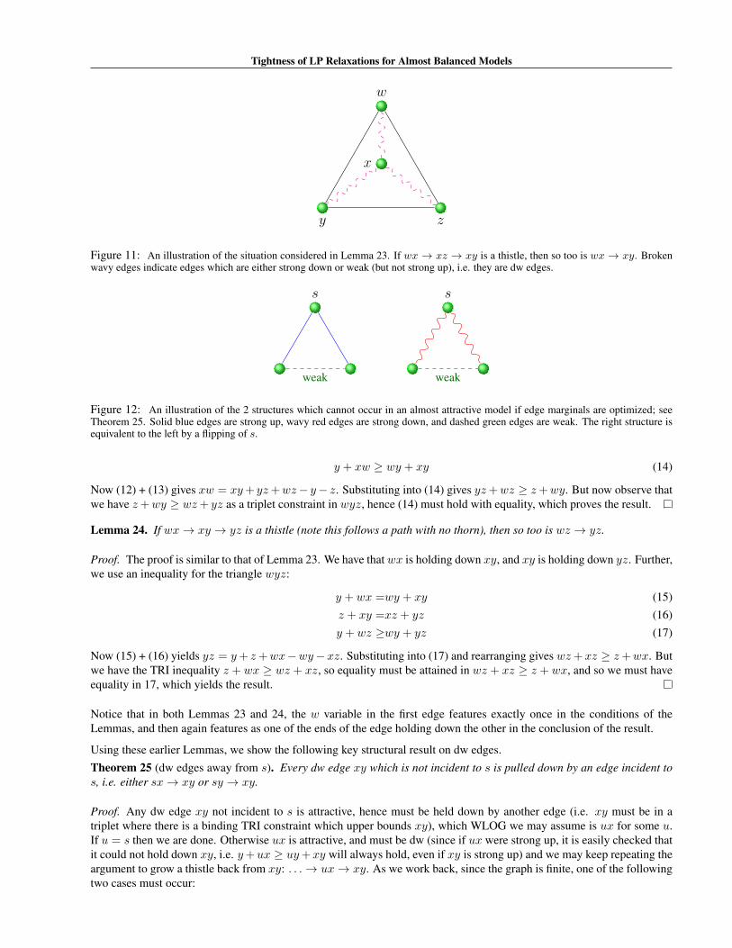
Tightness of LP Relaxations for Almost Balanced Models
w
y z
x
Figure 11: An illustration of the situation considered in Lemma 23. If wx → xz → xy is a thistle, then so too is wx → xy. Brokenwavy edges indicate edges which are either strong down or weak (but not strong up), i.e. they are dw edges.
s
weak
s
weak
Figure 12: An illustration of the 2 structures which cannot occur in an almost attractive model if edge marginals are optimized; seeTheorem 25. Solid blue edges are strong up, wavy red edges are strong down, and dashed green edges are weak. The right structure isequivalent to the left by a flipping of s.
y + xw ≥ wy + xy (14)
Now (12) + (13) gives xw = xy+ yz+wz− y− z. Substituting into (14) gives yz+wz ≥ z+wy. But now observe thatwe have z+wy ≥ wz+ yz as a triplet constraint in wyz, hence (14) must hold with equality, which proves the result.
Lemma 24. If wx→ xy → yz is a thistle (note this follows a path with no thorn), then so too is wz → yz.
Proof. The proof is similar to that of Lemma 23. We have thatwx is holding down xy, and xy is holding down yz. Further,we use an inequality for the triangle wyz:
y + wx =wy + xy (15)z + xy =xz + yz (16)y + wz ≥wy + yz (17)
Now (15) + (16) yields yz = y+ z+wx−wy−xz. Substituting into (17) and rearranging gives wz+xz ≥ z+wx. Butwe have the TRI inequality z + wx ≥ wz + xz, so equality must be attained in wz + xz ≥ z + wx, and so we must haveequality in 17, which yields the result.
Notice that in both Lemmas 23 and 24, the w variable in the first edge features exactly once in the conditions of theLemmas, and then again features as one of the ends of the edge holding down the other in the conclusion of the result.
Using these earlier Lemmas, we show the following key structural result on dw edges.Theorem 25 (dw edges away from s). Every dw edge xy which is not incident to s is pulled down by an edge incident tos, i.e. either sx→ xy or sy → xy.
Proof. Any dw edge xy not incident to s is attractive, hence must be held down by another edge (i.e. xy must be in atriplet where there is a binding TRI constraint which upper bounds xy), which WLOG we may assume is ux for some u.If u = s then we are done. Otherwise ux is attractive, and must be dw (since if ux were strong up, it is easily checked thatit could not hold down xy, i.e. y+ux ≥ uy+xy will always hold, even if xy is strong up) and we may keep repeating theargument to grow a thistle back from xy: . . .→ ux→ xy. As we work back, since the graph is finite, one of the followingtwo cases must occur:

Adrian Weller, Mark Rowland, David Sontag
1. We eventually hit an edge incident to s. The result then follows by repeatedly applying Lemmas 23 or 24.
2. We have a sub-thistle, the edges of which form a chordless cycle in the graph of length k ≥ 3, a1a2 → a2a3 →· · · aka1. Now repeatedly apply Lemmas 23 or 24 alternately to the sub-thistle given by the first three edges untilwe obtain either: a1ak → ak−1ak → aka1 or a1ak−1 → ak−1ak → aka1. In either case, this implies two tighttriangle inequalities in a1ak−1ak (this follows directly from the definition above of the → notation; for example,a1ak → ak−1ak → aka1 means ak−1 + a1ak = a1ak−1 + ak−1ak (from a1ak → ak−1ak) and also a1 + ak−1ak =a1ak−1 + a1ak (from ak−1ak → aka1)), which is a contradiction by Lemma 19.
Note that as a consequence of this Theorem, the two configurations shown in Figure 12 cannot occur.
We show a strengthening of the result if the dw edge is strong down.
Lemma 26 (Strong down edges away from s). If xy = 0 is a strong down edge with s /∈ {x, y}, then either: sx = x isstrong up and sy = 0 is strong down; or sx = 0 is strong down and sy = y is strong up.If xy > 0 is a strong down edge with s /∈ {x, y}, then either: sx = s is strong up and sy > 0 is strong down; or sx > 0 isstrong down and sy = s is strong up.
Proof. By Theorem 25, we have sx → xy or sy → xy. The remainder of the statement of the proof follows as astraightforward application of the relevant TRI constraint. We show the case xy = 0 and sx → xy: We have y + sx =sy + xy = sy. Rewrite this as (y − sy) + sx = 0. Both terms are ≥ 0 hence must both be exactly zero.
12 Specification of Complete Symmetric Perturbation (including all edges)
Throughout this Section, we assume an almost attractive model with special variable s, where edge marginals have beenoptimized over TRI given singleton marginals. Further, as justified by §9-10, we assume no locking edges or variables thathave singleton marginal 0 or 1.
We shall specify a perturbation for all singleton and all edge marginals with a number which is -1, 0 or 1 for each marginal.The perturbation up is formed by taking the vector of all these numbers and multiplying by a small ε. The perturbationdown is exactly the negative of the perturbation up. ε is to be chosen sufficiently small s.t. any constraint (this includes allTRI constraints, all LOC constraints, and all constraints on a marginal being ≥ 0 and ≤ 1) which was not tight initially,remains so after either perturbation. In order for both perturbations to remain in TRI, we shall demonstrate that all tightTRI constraints (and also all LOC constraints, see §12.2.1) are exactly maintained in all cases.
12.1 Rule for Singleton Marginals
The perturbation for the singleton marginal of the variable s is 0. For any other variable v ∈ V \ {s}, its perturbationdepends on its edge marginal to s, i.e. sv, according to the following exhaustive options (recall that we are assuming nolocking edges):
v moves by + 1 if v is strong up to s and v > s, or v is strong down to s and v + s < 1
v moves by − 1 if v is strong up to s and v < s, or v is strong down to s and v + s > 1
v moves by 0 if v has a weak edge to s.(18)
We remark that this perturbation has the appealing property that it maps to itself (actually it maps to the negative of itself,but that is equivalent since we perturb up and down) under a flipping of s (if a perturbation works for all almost attractivemodels, then the version obtained from it by flipping s must also work for all almost attractive models, since flipping s is abijection from the set of all almost attractive models to itself).
12.2 Rule for Edge Marginals
Given the changes in (18) for singleton marginals, we now show the perturbation for edge marginals.

Tightness of LP Relaxations for Almost Balanced Models
s
u vδ(uv) = 0
(a) su, sv weak
s
u v
u
δ(uv) = −1
(b) su = u, sv weak
s
u v
s
δ(uv) = 0
(c) su = s, sv weak
s
u v
s0
δ(uv) = +1
(d) su = 0 and sv = s
s
u v
0
δ(uv) = +1
(e) su = 0, sv weak
s
u v
s+u-1
δ(uv) = 0
(f) su = s+ u− 1, sv weak
s
u v
vs+u-1
δ(uv) = −1
(g) su = s+ u− 1 and sv = v
Figure 13: Cases where a weak edge uv is not incident to s. By Theorem 25, there must be a tight TRI constraint insuv. Here we show the possible forms with the implied perturbation for the weak edge. Note that the forms in the lowerrow may each by obtained from an appropriate form in the upper row by flipping s, so need not be considered separately.Specifically, under flipping s we have a↔ a, b↔ e, c↔ f, d↔ g.
12.2.1 Strong Edges
If an edge is strong (i.e. a LOC constraint is tight), we may immediately determine the perturbation required in order thatLOC constraints are respected for both perturbations up and down. Specifically:{
uv moves with min(u, v) if uv is strong upuv moves with max(0, u+ v − 1) if uv is strong down.
(19)
12.2.2 Note on Consistency, Remaining within TRI
The above rules clearly ensure that our perturbed marginals remain in LOC. Note that for any edge that had a tight LOCconstraint, i.e. was strong, the above rules exactly maintain this constraint when perturbed. We adopt this idea to ensurethat we shall also remain in TRI. That is, for our perturbed marginals to be in TRI, it is clearly sufficient if we ensure thatevery TRI constraint that was tight, is exactly maintained for the perturbed marginals. In order to demonstrate that ourperturbation satisfies this condition, we shall explicitly prescribe all perturbations for all weak edges, and show that ourprescribed perturbation exactly maintains all TRI constraints that are tight. In order to do this, we shall have to demonstratethat our prescribed changes for edges are consistent with the change that is necessary in all other triplets to preserve tightTRI constraints. This is what we mean by consistency, which we explore fully in §13.
12.2.3 Weak Edges Incident to s
The perturbation for a weak edge sw incident to s is -1. This is chosen since it is necessary to ensure consistency for anyTRI constraint involving the weak edge and any 2 strong edges, as we show in §13.2.1.
Note that we have now specified all edges (weak and strong) incident to s.
12.2.4 Weak Edges Not Incident to s, δ Notation
Given the above specifications, we may now use Theorem 25 to prescribe the change necessary for any weak edge uv notincident to s in order to maintain consistency. We adopt the notation δ(v) ∈ {−1, 0,+1} for the perturbation of a singletonmarginal v, and δ(uv) ∈ {−1, 0,+1} for the perturbation of an edge marginal uv. There are exactly 7 possible cases toconsider. In each case, it is straightforward to compute the required perturbation for the weak edge not incident to s, asshown in Figure 13. We provide more detail below.
If a weak edge uv is not incident to s, then by Theorem 25 it lies in a tight triangle with s, and as described in §12.2.4,we may deduce its necessary edge perturbation by considering the tight TRI constraint in the triangle suv. The 7 possiblecases are shown in Figure 13(a)-(g).
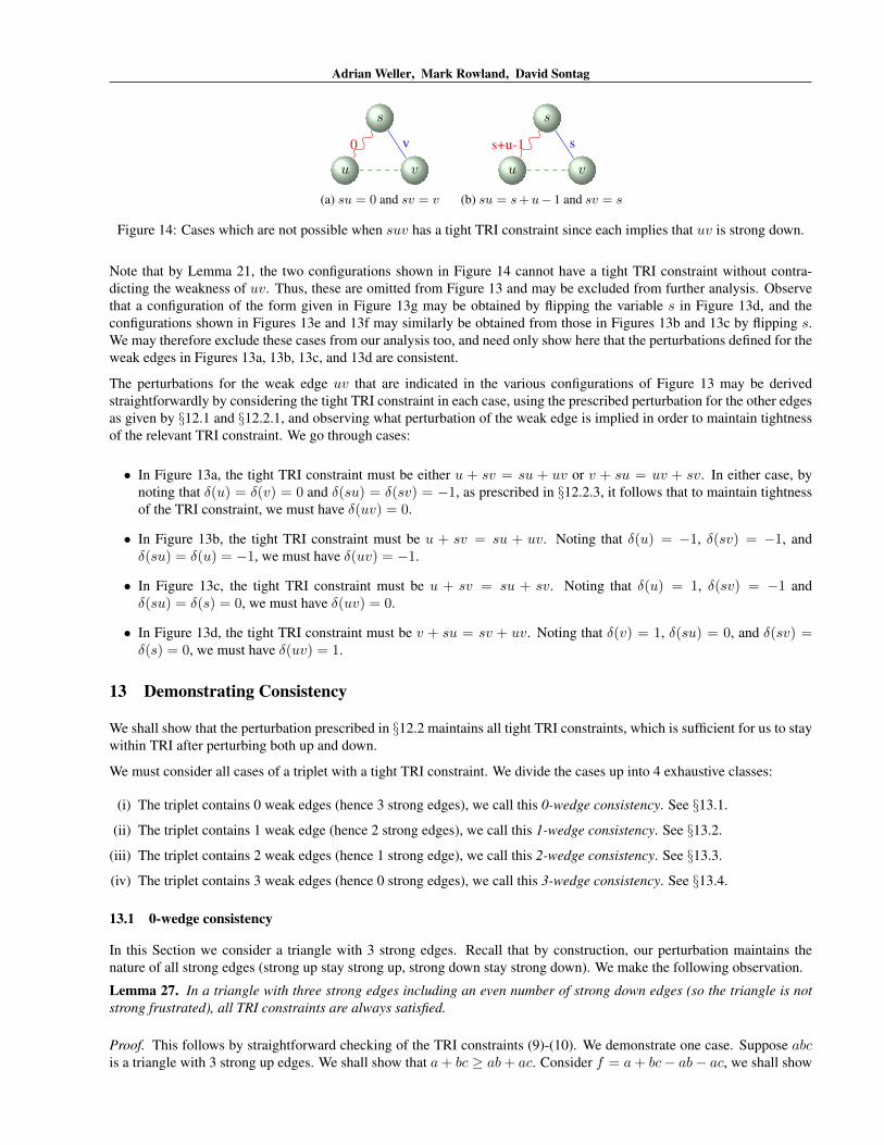
Adrian Weller, Mark Rowland, David Sontag
s
u v
v0
(a) su = 0 and sv = v
s
u v
ss+u-1
(b) su = s+u− 1 and sv = s
Figure 14: Cases which are not possible when suv has a tight TRI constraint since each implies that uv is strong down.
Note that by Lemma 21, the two configurations shown in Figure 14 cannot have a tight TRI constraint without contra-dicting the weakness of uv. Thus, these are omitted from Figure 13 and may be excluded from further analysis. Observethat a configuration of the form given in Figure 13g may be obtained by flipping the variable s in Figure 13d, and theconfigurations shown in Figures 13e and 13f may similarly be obtained from those in Figures 13b and 13c by flipping s.We may therefore exclude these cases from our analysis too, and need only show here that the perturbations defined for theweak edges in Figures 13a, 13b, 13c, and 13d are consistent.
The perturbations for the weak edge uv that are indicated in the various configurations of Figure 13 may be derivedstraightforwardly by considering the tight TRI constraint in each case, using the prescribed perturbation for the other edgesas given by §12.1 and §12.2.1, and observing what perturbation of the weak edge is implied in order to maintain tightnessof the relevant TRI constraint. We go through cases:
• In Figure 13a, the tight TRI constraint must be either u + sv = su + uv or v + su = uv + sv. In either case, bynoting that δ(u) = δ(v) = 0 and δ(su) = δ(sv) = −1, as prescribed in §12.2.3, it follows that to maintain tightnessof the TRI constraint, we must have δ(uv) = 0.
• In Figure 13b, the tight TRI constraint must be u + sv = su + uv. Noting that δ(u) = −1, δ(sv) = −1, andδ(su) = δ(u) = −1, we must have δ(uv) = −1.
• In Figure 13c, the tight TRI constraint must be u + sv = su + sv. Noting that δ(u) = 1, δ(sv) = −1 andδ(su) = δ(s) = 0, we must have δ(uv) = 0.
• In Figure 13d, the tight TRI constraint must be v + su = sv + uv. Noting that δ(v) = 1, δ(su) = 0, and δ(sv) =δ(s) = 0, we must have δ(uv) = 1.
13 Demonstrating Consistency
We shall show that the perturbation prescribed in §12.2 maintains all tight TRI constraints, which is sufficient for us to staywithin TRI after perturbing both up and down.
We must consider all cases of a triplet with a tight TRI constraint. We divide the cases up into 4 exhaustive classes:
(i) The triplet contains 0 weak edges (hence 3 strong edges), we call this 0-wedge consistency. See §13.1.
(ii) The triplet contains 1 weak edge (hence 2 strong edges), we call this 1-wedge consistency. See §13.2.
(iii) The triplet contains 2 weak edges (hence 1 strong edge), we call this 2-wedge consistency. See §13.3.
(iv) The triplet contains 3 weak edges (hence 0 strong edges), we call this 3-wedge consistency. See §13.4.
13.1 0-wedge consistency
In this Section we consider a triangle with 3 strong edges. Recall that by construction, our perturbation maintains thenature of all strong edges (strong up stay strong up, strong down stay strong down). We make the following observation.
Lemma 27. In a triangle with three strong edges including an even number of strong down edges (so the triangle is notstrong frustrated), all TRI constraints are always satisfied.
Proof. This follows by straightforward checking of the TRI constraints (9)-(10). We demonstrate one case. Suppose abcis a triangle with 3 strong up edges. We shall show that a+ bc ≥ ab+ ac. Consider f = a+ bc− ab− ac, we shall show

Tightness of LP Relaxations for Almost Balanced Models
s
c
a0
(a) a > s, c
s
c
a> 0
(b) a < s, c
b
c
a0
(c) a > b, c
b
c
a> 0
(d) a < b, c
Figure 15: The four possible types of triangles abc with one strong down edge bc and two strong up edges to consider for0-wedge consistency. We have a+ bc = ab+ ac, either a > bc with bc = 0, or a < b, c with bc > 0. On the left we havethe cases where s is in the triangle. See §13.1.
f ≥ 0. We have f = a + min(b, c) − min(a, b) − min(a, c), clearly symmetric in b and c, thus we may consider just 3subcases:
a ≤ b ≤ c ⇒ f = a+ b− a− a = b− a ≥ 0
b ≤ a ≤ c ⇒ f = a+ b− b− a = 0
b ≤ c ≤ a ⇒ f = a+ b− b− c = a− c ≥ 0.
Hence we need consider only triangles that are strong frustrated. We may rule out 3 strong down edges.
Lemma 28. A triangle with 3 strong down edges cannot occur.
Proof. Lemma 26 shows that s cannot be in such a triangle. Now applying Lemma 26 to each edge in turn around thetriangle yields a contradiction: we must alternate between strong up and strong down edges to s, yet this is not possiblesince we have an odd number of edges (if an edge is both strong up and strong down, one end must have marginal of 0 or1, which we are assuming cannot occur).
Thus we need consider only the case of a strong frustrated triangle abc that has 1 strong down edge bc and 2 strong upedges ab, ac, where a TRI constraint is tight. By Lemma 21, we must have a < b, c or a > b, c. It is easily checked that theonly TRI constraint of concern is where a+ bc = ab+ ac, hence we may assume that this holds. These are called problemtriangles of type (i) and (ii) in the main paper §4. Note that s could be b or c (in which case, we assume b WLOG) but nota by Lemma 26. See Figure 15 for illustrations of the four possibilities.
Considering first the cases where s is in the triangle. If a > s, c then we have δ(a) = +1, δ(sc) = 0, δ(sa) = δ(s) =0, δ(ac) = δ(c) = +1 ⇒ δ(a + sc − sa − ac) = 1 + 0 − 0 − 1 = 0 so we have consistency. If a < s, c thenδ(a) = −1, δ(sc) = δ(c) = −1, δ(sa) = δ(a) = −1, δ(ac) = δ(a) = −1⇒ δ(a+ sc− sa− ac) = −1− 1 + 1 + 1 = 0as required.
If s is not in the triangle then we may use Lemma 26 to give the edges from s to b and c, which determine their perturbations.WLOG we shall assume that sb is strong down and sc is strong up. It remains to determine the perturbation change to a,which we shall do by considering the edge sa.
If a > s, c (case c in Figure 15) then we have sb = 0, sc = c, ac = c. Also a+ bc = ab+ ac⇒ a = b+ c. From trianglesca we have c+ sa ≥ sc+ ac⇒ sa ≥ c+ c− c = c while from sba we have a+ bs ≥ ab+ sa⇒ sa ≤ a+ 0− b = c.Hence sa = c a weak edge. Now δ(a+ bc− ab− ac) = 0 + 0− 1 + 1 = 0 as required.
If a < s, c (case d in Figure 15) then we have sb > 0, sc = s, ac = ab = a. Also a + bc = ab + ac ⇒ a =b + c − 1. Applying the same TRI inequalities as in the last case, we obtain sa = s + b − 1, again a weak edge. Nowδ(a+ bc− ab− ac) = 0 + 0− 0 + 0 = 0 as required.
13.2 1-wedge consistency
We split the 1-wedge class into subclasses. We first consider in §13.2.1 the case that the 1 weak edge is incident to s. Thenin the following Sections, we demonstrate consistency exhaustively for all possible configurations of weak edges that arenot incident to s. These are illustrated in Figure 13. We need consider only cases shown in 13a to 13d, since the remainingcases may be obtained from these by flipping s.

Adrian Weller, Mark Rowland, David Sontag
s
w
v
s
w
v
Figure 16: The two possible types of triangles with one weak edge incident to s
s
w
v
0
v
s
w
v
s+v-1
w
Figure 17: Possible cases where there is a weak edge incident to s in a triangle with one strong up and one strong downedge, with a tight TRI constraint
13.2.1 Perturbation of a weak edge incident to s consistent with a TRI including 2 strong edges
As in §12.2.3, let sw be a weak edge incident to s. Recall that we prescribed δ(sw) = −1. Here we shall consider anypossible triangle involving a third variable v with sv and vw strong, and demonstrate consistency.
By Lemma 26, vw cannot be a strong down edge, hence vw must be strong up. There are therefore two cases to consider:(i) both sv and vw are strong up; and (ii) sv is strong down, and vw is strong up. See Figure 16.
We first consider case (ii). By Lemma 21, because sw is weak, we must have one of the 2 subcases shown in Figure 17.The only possible tight TRI constraint, which must therefore apply, is w + sv = sw + vw.
In order to maintain this TRI constraint through the perturbations, we must have
δ(w) + δ(sv) = δ(sw) + δ(vw).
Using our rules for perturbation from §12.1 and §12.2.1, in both subcases this gives δ(sw) = −1 which is consistent withour rule in §12.2.3.
We now consider case (i) where sv and sw are both strong up. The only possible tight TRI constraint, which must hold, isv+ sw = sv+ vw. By Lemma 21, we must have either v < s,w or v > s,w, see Figure 18. In either case, to preserve thetightness of the TRI constraint, following our rules for perturbation from §12.1 and §12.2.1, we must have δ(sw) = −1,which is consistent with our rule in §12.2.3.
13.2.2 1-wedge consistency of weak edge perturbations defined in Figure 13a
Here we prove that for any weak edge uv of the form appearing in Figure 13a, if there exists another variable x such thatuvx is a triangle with a tight TRI constraint, and ux, vx are strong edges, then the tight TRI constraint is maintained theprescribed perturbation for uv. This scenario is illustrated in Figure 19.
First note that by Lemma 26, ux and vx cannot be strong down. Therefore the only scenario to consider in this case iswhen ux and vx are strong up. Recall from Lemma 21, we must have either x < u, v or x > u, v. Note also that we havethe prescribed perturbations δ(u) = δ(v) = δ(uv) = 0. Since the only possible tight TRI constraint in uvx that does notcontradict the weakness of uv is x + uv = ux + vx, this equality must hold. By considering Figure 20, note that in eachcase, we must prove that δ(x) = 0 in order for tightness of this constraint to be maintained. Thus, it is sufficient in each
s
w
v
v
v
s
w
v
s
w
Figure 18: Possible cases where there is a weak edge incident to s in a triangle with two strong up edges, with a tight TRIconstraint

Tightness of LP Relaxations for Almost Balanced Models
s
u v
x
Figure 19: The consistency case to be analyzed in this section. Black zigzag lines indicate generic strong edges.
s
u v
x
u v
(a)
s
u v
x
x x
(b)
Figure 20: The possible configurations of the model shown in Figure 19
case to prove that sx is weak.
First, we consider x > u, v - see Figure 20a. In the tight triangle suv, one of the TRI constraints u + sv ≥ su + uv andv + su ≥ sv + uv must be tight; without loss of generality, we take u + sv = su + uv. In the tight triangle uvx, it mustbe the case that the tight TRI constraint is x + uv = ux + vx. From these two equations, we obtain x = v − sv + su.Now considering TRI inequalities in svx, we note v + sx ≥ sv + vx, so v + sx ≥ sv + v, and so sx ≥ sv. We also havex+ sv ≥ sx+ vx, which leads to su ≥ sx (by using the fact that x = v + su− sv). So we obtain
min(s, x) ≥ min(s, u) > su ≥ sx ≥ sv > 0
Therefore if we can show that sx 6= s+ x− 1, we have that sx is weak, so that δ(x) = 0, and so the tight TRI constraintx + uv = ux + vx is maintained under the perturbation, as we set out to show. To show this, suppose sx = s + x − 1,and consider the TRI constraint u + sx ≥ su + ux. Substituting in our expression for x, we obtain s + v − 1 ≥ sv,contradicting weakness of sv. Therefore sx is weak, and δ(x) = 0, as required.
Next, we consider x < u, v, as in Figure 20b. Again, for the tight TRI constraint in suv we may assume without loss ofgenerality that u + sv = su + uv. The only TRI constraint that can be tight in uvx (without contradicting weakness ofuv) is x+ uv = ux+ vx, which implies uv = x, so x = u+ sv − su. Considering the TRI constraint u+ sx ≥ su+ uxgives sx ≥ sv, and considering the TRI constraint x+ sv ≥ sx+ vx gives sv ≥ sx. Therefore we have sv = sx, and soimmediately we have sx > 0 and sx < s. We now just need to rule out sx = s + x − 1 and sx = x. If sx = s + x − 1,then by considering the TRI constraint v + sx ≥ vx + sv, we obtain sv ≤ s + v − 1, contradicting weakness of sv. Ifsx = x, then we obtain su = u is strong up, a contradiction.
13.2.3 1-wedge consistency of weak edge perturbations defined in Figure 13b
Here we prove that for any weak edge uv of the form appearing in Figure 13b, if there exists another variable x such thatuvx is a triangle with a tight TRI constraint, and ux, vx are strong edges, then the tight TRI constraint is maintained theprescribed perturbation for uv. This scenario is illustrated in Figure 21.
First, we note that xv cannot be strong down, by Lemma 26. Therefore we take xv strong up. Note also that since u < s,if ux is strong down, then it has edge marginal 0 and sx is strong down with edge marginal 0 too. Recall also that if ux isstrong up, then by Lemma 21 we have x > u, v or x < u, v. Figure 22 illustrates these cases.
In Figure 22a, note that the tight TRI constraint in uvx must be v + ux = uv + vx. Noting that in this case, we haveδ(v) = 0, δ(ux) = 0, δ(uv) = −1, if v > x, then δ(vx) = δ(x) = −1 (so the tightness of the TRI constraint ismaintained). If v < x, then the TRI constraint v + sx ≥ xv + sv, implies sv = 0, a contradiction.

Adrian Weller, Mark Rowland, David Sontag
s
u v
x
u
Figure 21: The consistency case to be analyzed in this section. Black zigzag lines indicate generic strong edges.
s
u v
x
u
0 0
(a)
s
u v
x
u
u v
(b)
s
u v
x
u
x x
(c)
Figure 22: The possible configurations of the model shown in Figure 21
In Figure 22b, note that the only possible tight TRI constraint in uvx is x+ uv = ux+ vx (all other contradict weaknessof uv). Note also that u+ sv = su+ uv is the only possible tight TRI constraint in suv, so sv = uv. Lastly, we have theTRI constraint x+ sv ≥ sx+ vx. But x+ sv = u+ v, so u ≥ sx. But considering the TRI constraint u+ sx ≥ su+ uxgives sx ≥ u. So sx = u is weak. So we have δ(x) = 0, δ(u) = −1, δ(v) = 0, and δ(uv) = −1, so the tightness ofx+ uv = ux+ vx is maintained.
In Figure 22c, note that by considering the TRI constraint u+sx ≥ ux+su, we obtain sx = x. We then note that the tightTRI constraint in uvxmust be x+uv = ux+vx (all others contradict the weakness of uv). Note that we have δ(x) = −1,δ(uv) = −1, δ(ux) = −1, and δ(vx) = −1, so the tightness of the TRI constraint is maintained.
13.2.4 1-wedge consistency of weak edge perturbations defined in Figure 13c
Here we prove that for any weak edge uv of the form appearing in Figure 13c, if there exists another variable x such thatuvx is a triangle with a tight TRI constraint, and ux, vx are strong edges, then the tight TRI constraint is maintained bythe prescribed perturbation for uv. This scenario is illustrated in Figure 23.
First, we note that xv cannot be strong down, by Lemma 26. Therefore we take xv strong up. Note also that since u < s,if ux is strong down, then it has edge marginal u+ x− 1 and sx is strong down with edge marginal 0 too. Recall also thatif ux is strong up, then by Lemma 21 we have x > u, v or x < u, v. Figure 24 illustrates these cases.
In Figure 24a, note that if vx = x, then by considering the TRI constraint v + sx ≥ sv + xv implies that sv is strongdown, a contradiction. So vx = v. Note that the only possible tight TRI constraint in uvx is v + ux = uv + vx, and wehave δ(v) = 0, δ(uv) = 0, δ(vx) = 0, and δ(ux) = 0, so the TRI constraint remains tight.
s
u v
x
s
Figure 23: The consistency case to be analyzed in this section. Black zigzag lines indicate generic strong edges.

Tightness of LP Relaxations for Almost Balanced Models
s
u v
x
s
u+x-1 s+x-1
(a)
s
u v
x
s
u v
(b)
s
u v
x
s
x x
(c)
Figure 24: The possible configurations of the model shown in Figure 23
s
u v
x
0 s
Figure 25: The consistency case to be analyzed in this section. Black zigzag lines indicate generic strong edges.
In Figure 24b, note that from the TRI constraint u+ sx ≥ su+ ux, we obtain sx ≥ s, and so sx = s. The only possibletight TRI constraint in uvx is x+uv = ux+vx (all others contradict the weakness of uv). But then note we have δ(x) = 1,δ(ux) = 1, δ(vx) = 0 and δ(uv) = 0, so the TRI constraint remains tight.
In Figure 24c, note that the only possible tight TRI constraint in uvx is x + uv = ux + vx (all others contradict theweakness of uv), so we obtain uv = x. Note that u + sx ≥ su + ux, so sx ≥ s + x − u. Also, x + sv ≥ sx + vx,so sv ≥ sx. But the only possible tight TRI constraint in suv is u + sv = su + uv, and this yields s + x − u ≥ sx, sosx = s+ x− u. Note this quantity is less than s and x, so sx not strong up; it is greater than s+ x− 1, and if it is equal to0, then we have sv = 0, a contradiction. Therefore sx is weak. From this, note that δ(x) = 0, δ(ux) = 0, δ(vx) = 0 andδ(uv) = 0, so the TRI constraint in uvx remains tight.
13.2.5 1-wedge consistency of weak edge perturbations defined in Figure 13d
In this section, we prove that for any weak edge uv of the form appearing in Figure 13d, if there exists another variablex such that uvx is a triangle with a tight TRI constraint, and ux, vx are strong edges, then the tight TRI constraint ismaintained the prescribed perturbation for uv. This scenario is illustrated in Figure 25.
There are three separate realizations of the scenario in Figure 25 to consider; see Figure 26.
Firstly, the case where ux is strong down - this is illustrated in Figure 26a. Since ux is incident to us, which has edgemarginal 0, ux = 0 too, by Lemma 26. Again by Lemma 26, sx is strong up and equal to x. Applying the TRI constraints+ xv ≥ sx+ sv yields vx ≥ x, so vx = x and is strong up. Finally, checking which TRI constraint can hold in the tighttriangle uvx, we note that the only possibility not contradicting the weakness of uv is v + ux = uv + vx, which leads tos = x, so we have a locking component and need not consider this example further.
Secondly, we consider ux, vx strong up; see Figures 26b-26c. Recall from Lemma 21 that we need only consider x < u, vand x > u, v. First consider x < u, v. The only TRI constraint in uvx that can be tight without contradicting the weaknessof uv is x+ uv = xu+ xv, so uv = x. But from the tight TRI constraint in usv, we get uv = v − s, so x = v − s. Nowconsidering the TRI constraint v + sx ≥ vs + vx gives sx = 0. Therefore we have δ(x) = 1, δ(uv) = 1, δ(xv) = 1,δ(xu) = 1, and verify that the constraint x + uv = xu + xv remains tight under the perturbation. If x > u, v, thenconsidering v + sx ≥ vs+ vx gives sx = s, so again we obtain δ(x) = 1, δ(uv) = 1, δ(xv) = 1, δ(xu) = 1, and verifythat the TRI constraint remains tight under the perturbation.
Finally, we consider ux strong up and vx strong down; see Figure 26d. vx strong down implies that sx strong down, andsv = s implies that both sx and vx are strong down with edge marginal greater than 0. The only TRI constraint in uvx thatcan be tight without contradicting the weakness of uv is u+ vx = uv+ ux. This implies ux = x+ (u+ v− 1− uv) < x

Adrian Weller, Mark Rowland, David Sontag
s
u v
x
x = s
0
0s
s
v-s
x
(a)
s
u v
x
0
x x
s
v-s
0
(b)
s
u v
x
0
u v
s
v-s
s
(c)
s
u v
x
v = 1− s
0
u x+v-1
s
v-s
s+x-1
(d)
Figure 26: The possible configurations of the model shown in Figure 25
s
u vδ(uv) = 0
Figure 27: su, sv weak and uv strong (of any type)
(as uv not strong down), so ux = u, and so uv = x+ v − 1. But note since v + su = sv + uv, we have uv = v − s, andso s = 1− x. Thus we have a locking component and need not consider this case further.
13.3 2-wedge consistency
13.3.1 The case where the 2 weak edges are both incident to s
This case is shown in Figure 27. The two possible tight TRI constraints are s + sv = uv + su or v + su = uv + sv. Ineither case, it is clear that we obtain a consistent conclusion that δ(uv) = 0 (consistent with δ(u) = δ(v) = 0 and hencethe strong edge uv does not move).
13.3.2 All other cases of 2-wedge consistency
For all these cases, we consider a tight triangle xyz away from s, with xy, yz, weak and xz strong. We note that by earlierarguments, sxy and syz must be triangles from Figure 13. Therefore it is sufficient to consider all pairs of triangles sxyand syz from Figure 13, and show that the tight TRI constraint in xyz remains tight under the perturbation. A priori thisgives 7 × 7 = 49 cases to check. However, by flipping s if necessary, sxy may always be taken to be one of a)-d) fromFigure 13, reducing the burden to 28 cases. We further note that by symmetry we always take sxy to be a triangle listedno later in Figure 13 than triangle syz - this rules out a further 6 cases to check. The remaining cases are exhaustivelyexamined below.
Note that the nature of the edge xz is not specified explicitly by the triangles sxy and syz. However, since in this sectionwe consider triangles xyz with exactly two weak edges, we do not consider the cases where xz is weak - these are coveredin §13.4.
In some cases, we will want to argue that certain combinations of tight TRI constraints and strong edges contradict ourassumptions that we have no locking edges, and/or our assumptions about which edges are weak. It is possible, butlaborious, to prove these contradictions of our assumptions algebraically; here we briefly explain a MATLAB script writtento verify these contradictions automatically, in the context of its use in §13.3.4. In this case, we wish to show that it cannotbe the case that sz = z, xz = z, all other edges weak, and z + sy = sz + yz, z + xy = xz + yz and y + sx = sy + xywithout our assumptions of no locking edges, or the weakness of the other edges, being contradicted. To do this, we runthe script shown at the top of Listing 1.
Listing 1: Example script used in this section>> equalities = {’z=sz’,’z=xz’,’z+sy’,’z+xy’,’y+sx’};
Tightness of LP Relaxations for Almost Balanced Models
% Test weak edges:testWeakness(equalities, ’sx’)testWeakness(equalities, ’sy’)testWeakness(equalities, ’xy’)testWeakness(equalities, ’yz’)% Test whether strong edges lock:testLocking(equalities, ’sz’, ’up’)testLocking(equalities, ’sx’, ’up’)
The variables equalities is a cell containing strings, which code for which LOC and TRI constraints we would liketo take to be tight. This gives rise to a new polytope, the restricted polytope given by intersecting TRI with all of theseconstraints. The function testWeakness examines a particular input edge uv in the graph to see whether it is alwaysstrong. This is implemented by checking whether any of the equations uv = 0, uv = u + v − 1, uv = u, uv = v alwayshold in the restricted polytope. All four equations are checked in a similar way; for example, to check whether uv = u atall points in the restricted polytope, two linear programs are set up to maximize and minimize the quantity uv− u over therestricted polytope. If the maximum and minimum are both found to be 0 (in practice, we use a threshold of 1e− 6), thenwe deduce that uv = u at all points in the polytope, and so we deduce that edge uv is forced to be strong, given the setof constraints assumed in the equalities variable. Similarly, the function testLocking checks whether a particularedge is locking up or down, by checking whether the two incident edge marginals are always equal (in the case of lockingup) or always sum to 1 (in the case of locking down) at all points in the restricted polytope; again, this is achieved bysetting up two linear programs to maximize and minimize a particular objective, and checking whether the maximum andminimum attained are equal.
Listing 2: Output generated by Listing 1Warning: The edge sy is actually strong up, with value y> In testWeakness (line 26)Warning: The edge xy is actually strong up, with value y> In testWeakness (line 26)Warning: The edge yz is actually strong up, with value y> In testWeakness (line 21)Warning: The edge yz is actually strong up, with value z> In testWeakness (line 26)
The output (see Listing 2) to the script listed in Listing 1 indicates which tested edges the program found to be lock-ing/strong. In particular, our assumption that sy is weak is shown to be contradicted by the set of TRI constraints weassumed to be tight; the program indicates that sy = y at all points in the restricted polytope, and so sy is actually impliedto be strong, a contradiction. This means we need not consider the case where our assumed set of TRI constraints holds. Asa point of interest, note that the output states that yz is forced to be equal to y and z at all points in the restricted polytope;this implies that yz is locked up, and this can indeed be verified, as demonstrated in Listing 3.
Listing 3: Demonstration of an edge which is noted to be forced into being locked up>> testLocking(equalities, ’yz’, ’up’)Warning: y and z are locked up> In testLocking (line 22)
This general approach allows us to deal efficiently with several of the checks described below. The code is available fromthe authors’ websites.
We indicate where this approach has been used below with the comment (verified via MATLAB program).
13.3.3 Case a)-a)
Consider the case where sxy and syz are both triangles of type 13a; see Figure 28 for an illustration. Note that xz cannotbe strong down, by Lemma 26. Therefore we may take xz strong up. Note that as sx, sy, sz are all weak, we haveδ(x) = δ(y) = δ(z) = 0. We also note from Figure 13a that δ(xy) = δ(yz) = 0. Finally, note also that δ(xz) = 0, as it

Adrian Weller, Mark Rowland, David Sontag
s
x
y
z
Figure 28: Model configuration for case a)-a)
s
x
y
z
z
Figure 29: Model configuration for case a)-b)
strong up and its incident variables do not move. Therefore whatever TRI constraint is tight in xyz, it remains tight afterthe perturbation, as all singleton and edge marginals do not move.
13.3.4 Case a)-b)
Consider the case where sxy is of type 13a and syz is of type 13b (so sz is the strong edge of the triangle syz); see Figure29 for an illustration. xz can’t be strong down by Lemma 26. So we may take xz strong up. We have δ(x) = 0, δ(y) = 0,δ(z) = −1, and δ(xy) = 0, δ(yz) = −1.
If z < x, note that this implies δ(xz) = δ(z) = −1. There are two possible TRI inequalities that could be tight in xyz.If x + yz = xy + xz, then note that this TRI constraint remains tight. If z + xy = xz + yz, then note in sxy, eitherx+ sy ≥ sx+ xy is tight - but then sx = x is strong up (verified via MATLAB program) - or y + sx ≥ sy + xy is tight -but then sy = y is strong up (verified via MATLAB program), so we need not consider these cases further.
If z > x, then consider triangle szx: x < z < s implies sx strong up by Lemma 21, so we need not consider this casefurther.
13.3.5 Case b)-b)
There are two ways in which triangles sxy and syz may be of type 13b; they may share either a weak edge incident to s,or a strong edge incident to s.
For the former, we consider sxy of type 13b (with sx strong), and syz of type 13b (with sz strong). xz can’t be strongdown by Lemma 26, so we may take xz strong up. We have δ(x) = −1, δ(y) = 0, δ(z) = −1, and δ(xy) = −1,δ(yz) = −1. Note that δ(xz) = −1 whether xz = x or xz = z. The two possible tight TRI inequalities in xyz arex + yz = xy + xz and z + yx = xz + yz. By symmetry of this case in x and z, it suffices to consider one of theseequations, and by substituting in the perturbations for each variable and edge, note that it remains tight.
For the latter, we consider sxy of type 13b and syz of type 13b, (with sy the strong edge in both triangles). xz cannot bestrong down by Lemma 26, so we may take xz strong up. We have δ(x) = 0, δ(y) = −1, δ(z) = 0, and δ(xy) = −1,δ(yz) = −1. Whether xz = x or xz = z, we have δ(xz) = 0. The two possible tight TRI inequalities in xyz arex + yz = xy + xz and z + yx = xz + yz. By symmetry of this case in x and z, it suffices to consider one of theseequations, and by substituting in the perturbations for each variable and edge, note that it remains tight.
13.3.6 Case a)-c)
We consider sxy of type 13a, syz of type 13c (so sz is the strong edge of the triangle). We have δ(x) = 0, δ(y) = 0,δ(z) = 1, and δ(xy) = 0, δ(yz) = 0. xz can’t be strong down by Lemma 26, so take xz strong up.
If xz = z, then consider triangle sxz, and note that s < z < x, implying sx strong up by Lemma 21, so we don’t need to
Tightness of LP Relaxations for Almost Balanced Models
s
x
y
z
x z
s
x
y
z
y
Figure 30: Model configurations for case b)-b)
s
x
y
z
s
Figure 31: Model configurations for case a)-c)
consider this case further.
If xz = x, then δ(xz) = δ(x) = 0. There are two possible tight TRI constraints in xyz. If x+yz = xy+xz, then pluggingin our singleton and edge perturbations immediately verifies this remains tight under the perturbation. If z+yx = yz+xz,then considering triangle sxy, we either have x + sy = xy + sx - in which case sx is strong up (verified via MATLABprogram) - or y+ sx = sy+ xy - in which case sy is strong up (verified via MATLAB program), so we need not considerthese cases further.
13.3.7 Case b)-c)
We consider sxy of type 13b (with sx strong) and syz of type 13c (with sz strong). We have δ(x) = −1, δ(y) = 0,δ(z) = 1, and δ(xy) = −1 and δ(yz) = 0. Note that xz cannot be strong down by Lemma 26, so take xz strong up.
If xz = z, then s >= x >= z >= s, so sx is locked up be Lemma 21, so we need not consider this case further.
IF xz = x, then δ(xz) = δ(x) = −1. There are two possible tight TRI constraints in xyz. If z+xy = yz+xz, then s andx are locked up (verified via MATLAB program). If x+ yz = xy+ xz, then s and z are locked up (verified via MATLABprogram), so we need not consider these cases further.
13.3.8 Case c)-c)
There are two ways in which triangles sxy and syz may be of type 13c; they may share either a weak edge incident to s,or a strong edge incident to s.
For the former, take sxy, syz of type 13c, with sx, sz strong. Note that xz cannot be strong down by Lemma 26, so takexz strong up. Either xz = x or xz = z. By symmetry of the model in x and z, it suffices to deal with xz = x. Then wehave δ(x) = 1, δ(y) = 0, δ(z) = 1, and δ(xy) = 0, δ(yz) = 0, and δ(xz) = 1. The tight TRI constraint in xyz is eitherx+ yz = xy + xz or z + xy = xz + yz, and in both cases the perturbation keeps the TRI constraint tight.
For the latter, take sxy, syz of type 13c, with sy = s strong. Note that xz cannot be strong down by Lemma 26, so takexz strong up. Either xz = x or xz = z. Again by symmetry of the problem in x and z, we need only consider xz = x.Then we have δ(x) = 0, δ(y) = 1, δ(z) = 0, and δ(xy) = 0, δ(yz) = 0, and δ(xz) = 0. There are two possible tight TRIconstraints, x + zy = xz + yz and z + xy = xz + xz - in both cases, no terms are perturbed, so the constraints remaintight.
13.3.9 Case a)-d)
It is not possible for triangles of type 13a and 13d to share an edge incident to s, so we need not consider this case.

Adrian Weller, Mark Rowland, David Sontag
13.3.10 Case b)-d)
It is not possible for triangles of type 13b and 13d to share an edge incident to s, so we need not consider this case.
13.3.11 Case c)-d)
We consider sxy of type 13c (with sy = s strong up) and syz of type 13d (with sz = 0 strong down). Note that xz cannotbe strong down by Lemma 26, so take xz strong up.
If xz = x, then by considering the TRI constraint x+ sz ≥ xz + sx, we obtain sx = 0 strong down, a contradiction.
If xz = z, then note that we have δ(x) = 0, δ(y) = 1, δ(z) = 1, and δ(xy) = 0, δ(yz) = 1, δ(xz) = 1. There are twopossible tight TRI constraints in xyz. If x + yz = xy + xz, then the above perturbation maintains the tightness of thisconstraint. If z + xy = xz + yz, this implies sx = 0 strong down (verified via MATLAB program), a contradiction.
13.3.12 Case d)-d)
There are two ways in which triangles sxy and syz may be of type 13d; they may share either a strong up edge incident tos, or a strong down incident to s.
For the former, we consider sxy, syz of type 13d (with sy the strong up edge). Note that xz cannot be strong down byLemma 26, so take xz strong up. So xz = x or xz = z; by symmetry in x and z, it suffices to consider xz = x. We haveδ(x) = δ(y) = δ(z) = 1, and δ(xy) = δ(yz) = δ(xz) = 1, so immediately it follows that any tight TRI constraint in xyzremains tight after the perturbation.
For the latter, we consider sxy, syz of type 13d (with sy the strong down edge). Again, we must have xz strong up, andby symmetry in x and z, it suffices to consider xz = x. Note that we have δ(x) = δ(y) = δ(z) = 1, and δ(xy) = δ(yz) =δ(xz) = 1, so immediately it follows that any tight TRI constraint in xyz remains tight after the perturbation.
13.3.13 Case a)-e)
We consider sxy of type 13a, and syz of type 13e (with sz the strong down edge). Note that under a flipping of s, this caseis the same as case a)-b).
13.3.14 Case b)-e)
We consider sxy of type 13b (with sx = x strong up), and syz of type 13e (With sz = 0 strong down). By consideringthe TRI inequality x + sz ≥ sx + xz, we note that xz = 0, and this TRI constraint is tight. The only possible tight TRIconstraint in xyz is y + xz = xy + yz (x + zy = xy + xz implies xy strong, z + xy = xz + yz implies yz strong,and xy + xz + yz = x + y + z − 1 implies s, x, z are locking (verified via MATLAB program)). We have δ(x) = −1,δ(y) = 0, δ(z) = 1, and δ(xy) = −1, δ(yz) = 1, δ(xz) = 0. Substituting these perturbations into the tight TRI constrainty + xz = xy + yz, we note tightness is maintained.
13.3.15 Case c)-e)
We consider sxy of type 13c (with sx = s strong up) and syz of type 13e (with sz = 0 strong down). Note that xz cannotbe strong down by Lemma 26, so take xz strong up.
If xz = x, then the TRI inequality x+ sz ≥ xs+ xz implies s = 0, so we need not deal with this case.
If xz = z, then the only possible tight TRI constraints are x + yz = xy + xz and z + xy = xz + yz, which both implythat sy is strong (verified via MATLAB program), so we need not deal with this case.
13.3.16 Case d)-e)
We consider sxy of type 13d (with sx = s strong up and sy = 0 strong down) and syz of type 13e (with sz = 0 strongdown). Note that xz cannot be strong down by Lemma 26, so take xz strong up.
If xz = x, then s < x < z, so so be Lemma 21 sx = s is strong up, so we need not consider this case further.
If xz = z, then we have δ(x) = 1, δ(y) = 1, δ(z) = 0, and δ(xy) = 1, δ(yz) = 1, δ(xz) = 0. There are two possibletight TRI constraints in xyz. If z+xy = xz+yz, then the perturbations described above maintain the tightness of the TRI

Tightness of LP Relaxations for Almost Balanced Models
constraint. If x+ yz = xy + xz, this forces sz to be strong up (verified via MATLAB program), so we need not considerthis case further.
13.3.17 Case a)-f)
We consider sxy of type 13a, and syz of type 13f (with sz the strong down edge). Note that under a flipping of s, this caseis the same as case a)-c).
13.3.18 Case b)-f)
We consider sxy of type 13b (with sx strong up), and syz of type 13f (with sz the strong down edge). Note that under aflipping of s, this case is the same as case c)-e).
13.3.19 Case c)-f)
We consider sxy of type 13c (with sx = s strong up), and syz of type 13f (with sz = s+ z − 1 strong down). If xz = x,then TRI inequality x + sz ≥ sx + sz implies that sz is strong up, a contradiction. By Lemma 26, xz cannot be strongdown and equal to 0. So the cases to consider are xz = z and xz = x+ z − 1.
If xz = z, then note δ(x) = 1, δ(y) = 0, δ(z) = −1, and δ(xy) = 0, δ(yz) = 0, δ(xz) = −1. There are two possible tightTRI constraints in xyz. If z + xy = xz + yz, then the perturbation described above maintains tightness of the constraint.If x+ yz = xy + xz, then xy is implied to be strong up (verified via MATLAB program), a contradiction.
If xz = x + z − 1, then the only TRI constraint that can be tight in xyz is y + xz = xy + yz (verified via MATLABprogram). This is maintained by the perturbation described above.
13.3.20 Case d)-f)
It is not possible for triangles of type 13d and 13f to share an edge incident to s, so we need not consider this case.
13.3.21 Case a)-g)
It is not possible for triangles of type 13a and 13g to share an edge incident to s, so we need not consider this case.
13.3.22 Case b)-g)
We consider sxy of type 13b (with sy = y strong up), and syz of type 13g (with sz = s+ z − 1 strong down). Note thatδ(x) = 0, δ(y) = −1, δ(z) = −1, and δ(xy) = −1, δ(yz) = −1. Note that xz cannot be strong down by Lemma 26, sotake xz strong up.
If xz = x, then δ(xz) = δ(x) = 0. The two possible tight TRI constraints in xyz are x+ yz = xy + xz (for which it canbe checked that the constraint remains tight with the perturbations specified above), and z + xy = xz + yz, which impliessx is strong down (verified via MATLAB program), a contradiction.
If xz = z, then δ(xz) = δ(z) = −1. The two possible tight TRI constraints in xyz are z+xy = xy+xz (for which it canbe checked that the constraint remains tight with the perturbations specified above), and x+ yz = xy+ xz, which impliessx is strong down (verified via MATLAB program), a contradiction.
13.3.23 Case c)-g)
It is not possible for triangles of type 13c and 13g to share an edge incident to s, so we need not consider this case.
13.3.24 Case d)-g)
It is not possible for triangles of type 13d and 13g to share an edge incident to s, so we need not consider this case.
13.4 3-wedge consistency
We now consider the case where a triangle xyz not incident to s has a tight TRI constraint, and demonstrate that this TRIconstraint remains tight when all singleton and edge marginals are perturbed according to the description given in §12.

Adrian Weller, Mark Rowland, David Sontag
x
z
s
y
(a) Case 1
x
z
s
y
s
(b) Case 2
x
z
s
y
x
(c) Case 3
x
z
s
y
s
0
(d) Case 4
x
z
s
y
x
s+y-1
(e) Case 5
Figure 32: The five cases to consider
We begin by arguing that we need check only 5 cases. First, the case where all edges sx, sy, sz are weak (Case 1). If twoof the edges sx, sy, sz are weak, then without loss of generality we make take sx strong. Note also that if sx strong down,this is obtained from a case where sx strong up by flipping s, so we only need to consider cases where sx is strong up(Cases 2 and 3). If exactly one of the edge sx, sy, sz are weak, then without loss of generality we may take sx, sy strong.It cannot be the case that both sx, sy are strong up or both strong down, as this would contradict Theorem 25, so withoutloss of generality we take sx strong up and sy strong down. As noted in §12.2.4, there are only two cases to consider;sx = s , sy = 0, and sx = x, sy = s+y−1; these form Cases 4 and 5. It cannot be the case that all three edges sx, sy, szare strong, since again this would contradict Theorem 25.
13.5 Case 1
All singleton and edge marginals have 0 perturbation, so any tight TRI constraint is preserved.
13.6 Case 2
We take sx = s, all other edges weak. We note that we have x + sz = sx + xz and x + sy = sx + xy. There must alsobe a tight constraint in syz holding yz down, by symmetry in y and z we may take it to be y + sz = sy + yz. We thenconsider the four possible TRI constraints that could be tight in xyz. If y+ xz = xy+ yz, then the perturbation maintainsthe tightness of this constraint. The other three constraints lead to contradictions of tight (verified via MATLAB program).
13.7 Case 3
We take sx = x, all other edges weak. We note that we have x+ sz = sx+ xz and x+ sy = sx+ xy. There must alsobe a tight constraint in syz holding yz down; by symmetry in y and z we may take it to be y + sz = sy + yz. There isalso a tight constraint in xyz by assumption. If it is y + xz = xy + yz, then the perturbation given for the singletons andedge marginals maintains the tightness of this constraint. The other three constraints lead to contradictions (verified viaMATLAB program).
13.8 Case 4
We take sx = s, sy = 0, and all other edges weak. We must have x + sz = sx + xz, x + sy = xy + sx, andz + sy = sz + yz. We consider the four possible TRI constraints that could be tight in xyz. If z + xy = xz + yz, thenthe perturbation given for the singletons and edge marginals maintains the tightness of this constraint. The other threeconstraints lead to contradictions (verified via MATLAB program).
13.9 Case 5
We take sx = x, sy = s + y − 1, and all other edges weak. We must have the TRI constrains x + sz = sx + xz,x + sy = xy + sx, and z + sy = sz + yz. We consider the four possible TRI constraints that could be tight in xyz. Ifz + xy = xz + yz, then the prescribed perturbation works. The other three constraints lead to contradictions (verified viaMATLAB program).

Tightness of LP Relaxations for Almost Balanced Models
14 Gathering Earlier Results to Provide Proofs of Theorems 8, 9 and 11
We gather together earlier results and use them to prove the following Theorems from the main paper.Theorem 8. For an almost balanced model, LP+TRI (the LP relaxation over TRI) is tight.Theorem 9. For an almost balanced model with special variable s, F sTRI(x) is a linear function.Theorem 11. In an almost balanced model with special variable s, if we fix qs = x ∈ [0, 1] and optimize in TRI over allother marginals, then an optimum is achieved with: qj ∈ {0, x, 1− x, 1} ∀j; all edges (other than to variables which have0 or 1 singleton marginal) are locked up or locked down, with no strong frustrated cycles.
We shall first prove Theorem 11 then use it to derive Theorem 9, after which Theorem 8 will easily follow.
Proof of Theorem 11, uses another simple perturbation. As before, we assume an almost attractive model and as justifiedby §9-10, we assume no locking edges or variables that have singleton marginal 0 or 1. We shall prove the result byshowing that, given these assumptions, the graph must have no variables other than s.
Given the results in §12-13, we have shown that if s is fixed while other marginals are optimized, then an optimum vertexcannot occur unless the perturbation defined in §12 does not exist, i.e. we know that all other variables have a weak edgeto s.
Hence, at an optimum vertex, there are no strong edges incident to s. In particular, there are no strong down edges incidentto s, and hence there are no strong down edges anywhere in the graph (by Lemma 26).
Since there are no strong down edges, it is now easily checked that the following perturbation (times a sufficiently small εs.t. all constraints which were not tight remain so) up and down preserves all tight LOC and TRI constraints:
s 0
v ∈ V \ {s} +1
sv edge, with v ∈ V \ {s} + 12
uv edge, with u, v ∈ V \ {s} +1.
Thus, it must be that at a vertex, all variables are either 0, 1 or in a locking component. This completes the proof ofTheorem 11.
Proof of Theorem 9. This is similar to the proof of Theorem 6. As there, we need only prove that F sTRI(x) is convex, thenlinearity follows from Lemma 5.
For any y ∈ [0, 1], consider an arg max of F iTRI(y) as given by Theorem 11. Partition the variables into 4 exhaustivesets: Ay = {j : qj = 0}, By = {j : qj = y}, Cy = {j : qj = 1 − y} and Dy = {j : qj = 1}. Define the functionfy : [0, 1]→ R given by fy(x) = f(q(x; y)) where q(x; y) is defined explicitly for singleton and edge marginals by:
qj(x; y) =
0 j ∈ Ayx j ∈ By1− x j ∈ Cy1 j ∈ Dy
, qij(x; y) =
0 i ∈ Ay or j ∈ Ayqi j ∈ Dy
qj i ∈ Dj
x i, j ∈ By1− x i, j ∈ Cy0 i ∈ By and j ∈ Cy; or i ∈ Cy and j ∈ By.
It is straightforward to check that always q(x; y) ∈ TRI (all edges are strong and there are no strong frustrated cycles).Observe that fy(x) is the linear function achieved by holding fixed the partition of variables Ay, By, Cy, Dy that wasdetermined for the arg max of the constrained optimum at qi = y. Now F iTRI(x) = supy∈[0,1] fy(x), hence is convex.
Note that, similarly to the remark after the proof of Theorem 6, we observe that each of the fy(x) functions in the proofmust be equal and hence the A,B,C,D sets may be taken to be constant with the same variables in them independent ofy.

Adrian Weller, Mark Rowland, David Sontag
Proof of Theorem 8. Given Theorem 9, it must be the case that a global optimum occurs at s = 0 or s = 1. If we conditionon either case, the remaining model is balanced, and the result follows from Theorem 2.
Following our results, strengthenings of Theorem 8 were shown (Weller, 2016a,b).