Tiebout’s Tale in Spatial Economies:Entrepreneurship, Self-Selection, and

Efficiency∗

Hideo Konishi†

November 30, 2007

Abstract

This paper establishes the existence and efficiency of equilibriumin a local public goods economy with spatial structures by formaliz-ing Hamilton’s (1975 Urban Studies) elaboration of Tiebout’s (1956JPE) tale. We use a well-known equilibrium concept from Rothschildand Stiglitz (1976, QJE) in a market with asymmetric information,and show that Hamilton’s zoning policy plays an essential role in prov-ing the existence and efficiency of equilibrium. We use an idealizedlarge economy following Ellickson, Grodal, Scotchmer and Zame (1999,Econometrica) and Allouch, Conley and Wooders (2004). Our theoremis directly applicable to the existence and efficiency of a discrete spa-tial approximation of mono- or multi-centric city equilibria in an urbaneconomy with commuting time costs, even if we allow the existence ofmultiple qualities of (collective) residences, when externalities due totraffic congestion are not present.

∗I thank Jan Brueckner, John Conley, Masa Fujita, Atsushi Kajii, Kazuya Kamiya, Se-ilMun, Jaime Luque, Frederic Robert-Nicoud, Alain Trannoy, and Myrna Wooders for theircomments and encouragements, and Frank Georges for his research assistance. I especiallythank two anonymous referees and an associate editor of the journal for their helpful com-ments and suggestions. My intellectual debt to Marcus Berliant is obvious. All errors are,of course, my own.

†Department of Economics, Boston College hideo.konishi@bc.edu

1

It is useful in closing to restate the problem as Samuelson (1954)sees it:

“However, no decentralized pricing system can serve to determineoptimally these levels of collective consumption. . . .”

It is the contention of this article that, for a substantial portionof collective or public goods, this problem does have a conceptualsolution. (Charles M. Tiebout, “A Pure Theory of Local PublicExpenditure,” Journal of Political Economy LXIV, 1956, p. 424)

1 Introduction

In his celebrated paper published a half century ago, Tiebout (1956) arguedthat although Samuelsonian pure public goods may be underprovided due toconsumers’ free-riding incentives in reporting preferences, examples of purepublic goods are very rare, and impure local public goods can be providedefficiently (efficiency) by consumers’ revealed preferences through voting withfeet (self-selection) and competition among jurisdictions (entrepreneurship).Recently, Ellickson, Grodal, Scotchmer, and Zame (1999)1 and Allouch,

Conley, and Wooders (2004) provide nice formalizations of Tiebout’s idea,proving the existence and Pareto efficiency of Tiebout equilibrium in the exactsense.2 According to these papers, if the number of jurisdictions is very large,there is no spillover effect across jurisdictions, jurisdiction managers maxi-mize profits, and the price system is complete for every possible jurisdictiontype, then: there exists a Tiebout equilibrium, and every Tiebout equilibrium

1As they say in their paper, Ellickson et al. (1999) deal with a club economy, in whichconsumers are allowed to join multiple clubs. However, if we impose a single-membershipconstraint, their model becomes a standard local public goods model with finite publicprojects and infinite consumer types. Allouch et al. (2004) deal with local public goodswith infinite public projects and finite consumer types.

2Wooders (1978, 1980) considers finite population cases. The former paper shows the ex-istence and efficiency of equilibrium in the exact sense when total population can be exactlydivided up into communities of optimal size. The latter shows the existence and efficiency(core convergence) of equilibrium in approximation for large finite economies. Ellickson etal. (1999) and Allouch et al. (2004), in contrast, show the existence and efficiency of equi-librium in the exact sense with a continuum of consumers when each jurisdiction populationis finite.

2

is Pareto efficient.3 They thus provide a rigorous theoretical foundation forTiebout’s tale.However, as are many papers in the literature that provide support for

Tiebout’s tale, these papers are still not satisfactory, in two ways, for theanalysis of a local public goods economy. First, they do not consider spatialelements.4 In his original paper, Tiebout says that housing developers’ actionsadjust the population of (suburban) communities to an efficient size.5 Sincesuburbanization and a voluntary sorting process make the case in the realworld for Tiebout’s tale, it seems important for any model to take into ac-count both spatial considerations and the actions of housing developers. Also,as pointed out by Hamilton (1975), in US suburbs, jurisdictions’ expensesare financed by property taxes, especially taxes on housing. Thus, the modelneeds to include land in order to justify Tiebout’s tale in the real world. Moreglobally, consumers may care about the climates and geographical featuresof locations (say, Boston or Los Angeles). Even within the same metropol-itan area, they may have preferences for the seaside or the mountains (say,in San Diego). Finally, Tiebout assumes that there is no restriction due toemployment opportunity.6 This is certainly a very strong assumption if weconsider modern American suburbs, where consumers undeniably consider thenearby job opportunities and commuting time when choosing where to live; itseems almost contradictory once spatial elements are introduced in the model.Thus, it is intriguing to know if Tiebout’s tale would work without such astrong assumption.Second, many papers in the literature including Ellickson et al. (1999) and

Allouch et al. (2004) assume (implicitly or explicitly) that the price system

3Bewley (1981) made thorough criticisms of Tiebout’s tale. By providing a sequenceof counterexamples, he argued convincingly that Tiebout’s tale is supportable only in atrivial local public service economy that is essentially the same as a private good economy.However, he assumes that the number of jurisdictions is finite. This is the main reason thatBewley (1981) obtains a very negative result.

4In the club goods model, spatial elements are less important than in the local publicgoods model. Thus, unless their theorem is applied to a local public goods economy, thefirst point does not apply to Ellickson et al. (1999). The second point (stated below) willbe relevant for both papers.

5Discussions after his Assumption 7. Assumption 7 states that “communities below theoptimum size seek to attract new residents to lower average costs. Those above optimal sizedo just the opposite. Those at an optimum try to keep their population constant.”

6His Assumption 4: “Restrictions due to employment opportunities are not considered.It may be assumed that all persons are living on dividend income.”

3

is complete: that is, there are markets for all potential jurisdiction types inaddition to the jurisdiction types that are observed in equilibrium. This isobviously an unrealistic and unsatisfactory assumption. In this paper, using anequilibrium concept from Rothschild and Stiglitz (1976), we successfully dropthe complete market assumption while preserving efficiency of equilibrium.We provide a spatial model and an equilibrium concept that answer the

above considerations. We show that these considerations in themselves do notspeak against Tiebout’s tale. We prove both existence and efficiency of equi-librium by extending the approaches of Ellickson et al. (1999) and Allouch etal. (2004). The key assumptions for our positive result are (i) a large numberof jurisdictions in each physical location; (ii) Hamilton’s (1975) zoning policywhich makes crowding effects fiscally anonymous; and (iii) free entry by po-tential profit-maximizing jurisdiction managers. We also show as a corollaryof our theorem that a closed-economy, finite-location monocentric city has anequilibrium even when quality of housing is a variable determined by devel-opers and collective houses (condos/apartments) are allowed, and that theequilibrium is efficient in the absence of externalities due to traffic congestion.In the rest of this section, we discuss the above two considerations in more

detail. In Section 2, we briefly explain how efficiency of equilibrium is achievedwith our equilibrium concept. In Section 3, we present our model, our conceptof equilibrium, and the result (Theorem). Section 4 provides the sketch ofthe proof. Section 5 closes the paper with possible extensions, applications tourban economics, and cautious remarks on the implications of our result.

1.1 Spatial Considerations

Several papers discuss efficiency of equilibrium while considering some of thefollowing spatial aspects: (i) the effects of property taxes and zoning policiesand (ii) differences in physical location and/or commuting costs.In the U.S., the main revenue source of local jurisdictions is property tax,

which is mainly a tax on housing values. In a beautiful but informal pa-per, Hamilton (1975) discusses efficiency and self-selection in equilibrium ofa model that includes housing developers and land. Hamilton argues that ifthe jurisdictions are profit-maximizing land developers, complete segregationby preferences and efficiency of equilibrium are achieved simultaneously if thejurisdictions adopt zoning policies (minimum lot size restrictions).7 A zoning

7A paper by Sonstelie and Portney (1978) is similar to Hamilton’s with some more details.

4

policy eliminates distortion, prevents free-riding, and achieves segregation ofconsumers by their preferences. This insightful story supplements Tiebout’soriginal tale and makes it applicable to spatial models.8

[Figure 1.]

We also introduce heterogeneous locations into the model so that we caninclude commuting costs and preferences over physical locations. We assumethat there are many jurisdictions in each physical location. Thus, within a ju-risdiction, land is assumed to be homogeneous (see Figure 1); our frameworkin the current paper cannot handle heterogeneous land within a jurisdiction.9

Note also that wage rates vary in different locations due to different levelsof productivity. As we have said above, Tiebout (1956) assumes that thereare no restrictions arising from employment opportunities (his assumption 4).Buchanan and Wagner (1970), Buchanan and Goetz (1972), and Flatters,Henderson, and Mieszkowski (1974) elaborate Tiebout’s statement by claim-ing that allowing individuals to choose their location of employment precludesefficiency of equilibrium since “voting with feet” is a process of utility equaliza-tion rather than one of marginal product equalization. However, these modelshave a predetermined finite number of jurisdictions, and do not allow for thepossibility of creating a new jurisdiction. In our model, there are many smalljurisdictions and entry of new jurisdictions is allowed implicitly. In such ascenario, we can show that spatial wage differentials play no role in achievingefficiency of equilibrium.

1.2 Equilibrium Concept

Besides spatial location, another point we address in this paper is the conceptof equilibrium. Although Ellickson et al. (1999) and Allouch et al. (2004) pro-vide positive results (existence and the first welfare theorem), their equilibriumconcepts assume that agents are price takers and that the market is completein the sense that every possible jurisdiction type (or jurisdiction policy pack-age: population, tax rate, and local public goods) has a price regardless of the

8In his footnote 15, Hamilton also says that zoning policy would achieve efficiency evenwith heterogeneous locations in the context of a monocentric city briefly.

9Henderson (1974) proposed a model of system of cities, in which there are many special-ized monocentric cities trading with each other. In contrast, our model deal with smallerjurisdictions, and there are many jurisdictions within a monocentric city.

5

Location 3

Type w jurisdiction

Type w’jurisdiction

Urban Layout: Monocentric City Case

Figure 1

CBD: Central Business District

Location 1

Location 2

member

CBD

.. . .... .

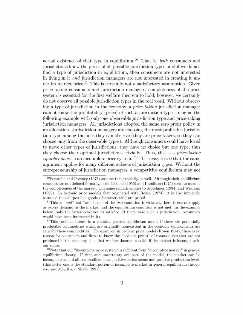
actual existence of that type in equilibrium.10 That is, both consumers andjurisdictions know the prices of all possible jurisdiction types, and if we do notfind a type of jurisdiction in equilibrium, then consumers are not interestedin living in it and jurisdiction managers are not interested in creating it un-der its market price.11 This is certainly not a satisfactory assumption. Givenprice-taking consumers and jurisdiction managers, completeness of the pricesystem is essential for the first welfare theorem to hold; however, we certainlydo not observe all possible jurisdiction types in the real word. Without observ-ing a type of jurisdiction in the economy, a price-taking jurisdiction managercannot know the profitability (price) of such a jurisdiction type. Imagine thefollowing example with only one observable jurisdiction type and price-takingjurisdiction managers: All jurisdictions adopted the same zero profit policy inan allocation. Jurisdiction managers are choosing the most profitable jurisdic-tion type among the ones they can observe (they are price-takers, so they canchoose only from the observable types). Although consumers could have lovedto move other types of jurisdictions, they have no choice but one type, thusthey choose their optimal jurisdictions trivially. Thus, this is a price-takingequilibrium with an incomplete price system.12 ,13 It is easy to see that the sameargument applies for many different subsets of jurisdiction types. Without theentrepreneurship of jurisdiction managers, a competitive equilibrium may not

10Sonstelie and Portney (1978) assume this explicitly as well. Although their equilibriumconcepts are not defined formally, both Tiebout (1956) and Hamilton (1975) seem to assumethe completeness of the market. The same remark applies to Scotchmer (1994) and Wildasin(1992). In hedonic price models that originated with Rosen (1974), it is also implicitlyassumed that all possible goods (characteristics) are priced.11This is “and” not “or.” If one of the two condition is violated, there is excess supply

or excess demand in the market, and the equilibrium condition is not met. In the examplebelow, only the latter condition is satisfied (if there were such a jurisdiction, consumerswould have been interested in it).12This problem occurs in a classical general equilibrium model if there are potentially

producible commodities which are originally nonexistent in the economy (endowments arezero for these commodities). For example, in hedonic price model (Rosen 1974), there is noreason for consumers and firms to know the “hedonic prices” of commodities that are notproduced in the economy. The first welfare theorem can fail if the market is incomplete inour sense.13Note that our "incomplete price system" is different from "incomplete market" in general

equilibrium theory. If time and uncertainty are part of the model, the market can beincomplete even if all commodities have positive endowments and positive production levels(this latter one is the standard notion of incomplete market in general equilibrium theory:see, say, Magill and Shafer 1991).

6

achieve efficiency.In contrast, Wooders (1978) and Bewley (1981) consider equilibrium con-

cepts in which prices are set only for existing jurisdiction types, and theyassume that a group of consumers can form a coalitional deviation to createan unavailable type of jurisdiction (entrepreneurial consumers). However, al-lowing such a coalitional deviation of consumers does not fit very well withTiebout’s original tale: unlike Samuelson’s pure public goods case, the marketmechanism can achieve efficient allocations in equilibria even if jurisdictionscannot observe each consumer’s preferences.14

In this paper, instead of assuming entrepreneurial consumers, we assumeentrepreneurial jurisdiction managers. We will use a version of the well-knownequilibrium concept defined for markets with asymmetric information (adverseselection) by Rothschild and Stiglitz (1976).15 We assume that a jurisdictionmanager does not know each consumer’s preference type (although she knowsthe distribution of their preference types), which is a more suitable assump-tion. An announced jurisdiction policy can attract only one type of consumeras resident if that type is the only one that derives higher utility from thepolicy than from currently available jurisdiction policies in the market. Theequilibrium concept employed here requires that: (i) no consumer have anincentive to move among existing jurisdictions, and that (ii) there be no un-available jurisdiction policy that can both attract consumers and be profitableto a jurisdiction manager. We call this Rothschild-Stiglitz type of equilibriumwith zoning policies a Tiebout equilibrium with entrepreneurial jurisdictions.We will show that this equilibrium concept is indeed sufficient to prove theexistence and efficiency of equilibrium.

14Recall the quote in the beginning of the paper. Another relevant quote is, “. . . Yet interms of a satisfactory theory of public finance, it would be desirable (1) to force the voterto reveal his preferences; (2) to be able to satisfy them in the same sense that a privategoods market does; and (3) to tax him accordingly.” (Tiebout, 1956, pp. 417-418.)15In Rothschild and Stiglitz (1976), there are low-risk and high-risk consumers, and insur-

ance companies compete with each other via their insurance plans in a competitive market(with free entry). Insurance companies cannot distinguish consumer types, although theyknow the distribution of consumer types. They show that equilibrium may fail to exist:when high-risks and low-risks choose the same plan an insurance firm has an incentive tooffer a plan that attracts only low-risks, whereas when two types choose different plans byself-selection, there may be a plan that attracts both.

7

2 The Mechanism of Achieving Efficiency

In this section, we show how Hamilton (1975), together with Rothschild andStiglitz (1976), supports Tiebout’s tale (1956). Hamilton’s zoning policy re-covers (existence and) efficiency of equilibrium under a property tax systemin two different ways: one is by supporting an efficient allocation by (dis-tortionary) property taxes, and the other by preserving fiscal anonymity ofcrowding in order to avoid the free-rider problem. First, Figure 2 shows thatproperty tax is distortionary unless a zoning policy is in place: point A is anefficient equilibrium while point B is the inefficient one. If zoning policies arenot in place, all consumers want to reduce their land consumption (point B).Note that if a zoning policy is not binding, then entrepreneurial jurisdictionsthat put in place zoning policies that are binding can make profits by removingdistortions. Hamilton’s zoning policy is essential in recovering efficiency of aTiebout equilibrium by eliminating distortions.16

[Figure 2.]

Second, and more important, a zoning policy also works as a tool that pre-vents free-rider problems. Suppose that rich people strongly prefer large landlots, while the poor prefer small lots if land is expensive. Then, if they live inthe same jurisdiction, the rich will need to pay a lot in property taxes, whilethe poor can enjoy local public goods for much less in property taxes. Thus,without zoning policies, a resident’s utility depends on the composition of thepopulation of her jurisdiction: i.e., congestion is not fiscally anonymous dueto property taxes. Pauly (1976) describes this problem as a “poor chasing therich” situation. Structurally this is exactly the problem faced by the insurancemarket in Rothschild and Stiglitz (1976). High-risk and low-risk consumerscorrespond to the poor and the rich in our model, respectively. As is wellknown in the literature, neither existence nor efficiency is guaranteed in insur-ance markets with the Rothschild-Stiglitz equilibrium (Rothschild and Stiglitz1976). However, Hamilton’s zoning policy makes tax payments equal in thesame jurisdiction (if the constraint binds), and congestion becomes anonymousin our local public goods economy.17 This is because zoning policy makes con-gestion under property tax fiscally anonymous (since every household in the16See Wheaton (1975). Wheaton (1975) says that Tiebout’s efficiency tale is incorrect

since property taxes are distortionary.17The Rothschild-Stiglitz equilibrium can be used for Rosen’s hedonic price models in the

same way without assuming a complete price system for all potential commodities.

8

Poll tax

Consum

ption

Land

Zoning constraint

Market prices

Budget constraint

with zoning

A B

A:

equilibriumland

consumption w

ith zoning. (H

amilton, 1975)

B:

equilibrium land

consumption w

ithout zoning.(W

heaton, 1975)

0Budget line w

ith property tax

Market prices

Market prices

Figure2

same jurisdiction needs to pay the same amount under the policy). This im-plies that cost of a public project in the jurisdiction is divided equally, and aproperty tax becomes essentially a poll tax.18

With this observation, our efficiency result can be easily shown. First, as-suming all types of jurisdictions (in public projects and the population), wefind a competitive equilibrium with poll taxes by letting each type of consumerchoose her most favorite jurisdiction type among all budget-balancing juris-diction types. We can show that this poll tax equilibrium is Pareto efficient byemploying McKenzie’s trading set approach (McKenzie 1959). Then, we canachieve our goal if we can prove that a Tiebout equilibrium with entrepreneur-ial jurisdictions is equivalent to the poll tax equilibrium. By our observation(Figure 1), it is easy to see that every poll tax equilibrium can be supported bya Tiebout equilibrium with entrepreneurial jurisdictions (a Rothschild-Stiglitzequilibrium with property taxes and zoning policies). The other direction isto show that every Tiebout equilibrium with entrepreneurial jurisdictions is apoll tax equilibrium. Here, condition (ii) of the equilibrium (of Rothschild andStiglitz 1976) plays an important role: there must be no unavailable jurisdic-tion policy that can both attract consumers and be profitable to a jurisdictionmanager. This is a free entry condition, and if an allocation is inefficient,an entrepreneurial jurisdiction manager can make profits by offering a policypackage to a particular type of consumer that is better than the packages cur-rently available in the market.19 This shows that every Tiebout equilibriumwith entrepreneurial jurisdictions must be an allocation in which each type istotally segregated and achieves the maximum payoff under segregations. Thisis a poll tax equilibrium. This is why we can derive the first welfare theoremfor a Tiebout equilibrium with entrepreneurial jurisdictions.In the rest of the paper, we formally define Tiebout equilibrium with en-

trepreneurial jurisdictions, and prove the existence and efficiency of the equi-

18Nechyba (1997) analyzes a local public good model with existing houses (thus, con-sumers can choose only from existing house/lot sizes). His setup resembles Hamilton’s(binding) zoning policies. The difference is that since new houses cannot be provided byjurisdiction managers in Nechyba’s case, the global Pareo efficient allocation cannot beachieved.19Indeed, in a Tiebout economy, Brueckner (1981) shows by an example that there may

be inefficient equilibria other than the efficient sorting equilibrium unless free entry of juris-dictions is assumed. Brueckner (1981) assumes a perfectly elastic land supply, which turnsout to be consistent with our infinitesimal jurisdiction assumption in the current paper.Bewley (1981) also stresses the importance of free entry.

9

librium.

3 The Model

The model assumes that there are finitely many physical locations in the econ-omy. The set of locations is denoted J , and its representative element is j ∈ J .These locations can differ in climate or in geographical features. Each loca-tion j has some quantity of land Lj > 0, i.e., each location has only a lim-ited amount of land to utilize. There is one numeraire commodity which canbe produced by labor at each location j ∈ J with constant-returns-to-scalelocation-specific technology: that is, the amount of labor needed to produceone unit of the numeraire commodity at location j ∈ J is constant and isdenoted αj, which can be dependent on j. At location j ∈ J , the prices ofprivately consumed goods – the numeraire commodity, land, and leisure –are 1, rj, and wj, respectively. Given the constant returns to scale technology,wjαj = 1. There is a finite number of possible public projects (see Mas-Colell,1980). Public projects are discrete public goods such as schools, parks, andwater supply systems, etc., and any combinations of them. The set of all pub-lic projects is denoted G, and its representative element is g ∈ G. Each publicproject g ∈ G can be produced by c(g) units of the numeraire commodity. Weassume that provision of no public project is always available for jurisdictionmanagers: ∅ ∈ G with c(∅) = 0 (no provision, so no cost).A type ω jurisdiction provides a public project and imposes a land tax

(property tax) on its residents. Each jurisdiction ω is characterized by itslocation jω ∈ J , public project gω ∈ G, total land size Lω, and (specific) landtax tω. In addition, jurisdictions can impose zoning constraints (Hamilton1975): i.e., the size of the lot for each household must be greater than or equalto ζω: z ≥ ζω (if no zoning constraint, ζω = 0). Although zoning constraintsare inequalities, in the equilibrium they will be binding, as we will see below(proof of Proposition 3; see also Figure 1). Thus, we will impose zoningconstraints as equalities for brevity of explanation: that is, a resident of typeω jurisdiction must consume ζω land. The total land size Lω is determinedby how many residents join the jurisdiction, and Lω = ζωnω follows underzoning requirement ζω, where nω is the number of households in a type ωjurisdiction. Thus, a type ω jurisdiction is characterized by its policy listω = (jω, gω, tω, ζω, nω). The set of all possible policy lists is denoted Ω =J ×G×R+ × R+ × Z++, where Z++ is the set of positive integers.

10

There is a finite number of types of consumers. The set of all types isdenoted Θ, and its representative element is θ ∈ Θ. A type θ consumer hasa location-specific utility function uθj : R+ × [0, θ

j ] × R+ × G × Z++ → Rfor each j ∈ J such that uθj(x, , z, g, n) denotes type θ’s utility who lives ina jurisdiction at location j that provides public project g with n residents,consuming numeraire, land, and leisure by x, z, and . We assume that thereis no spillover benefit of local public goods across jurisdiction borders. Withoutthis assumption, it is obvious that equilibrium efficiency is not attained withoutinternalizing such externalities. Type θ consumer can spend at most θ

j leisurehours at location j, where θ

j > 0 denotes type θ’s leisure endowment hoursat location j ∈ J .20 We assume that uθj is a continuous function. Type θconsumer is endowed with land vector (Lθ

j)j∈J ∈ RJ+. That is, a consumer’s

utility depends on private goods consumption x, z, and , public project g,and the level of congestion n as well as her choice of location j itself. However,under the provision of no public projects, g = ∅, congestion is assumed tobe irrelevant: uθj(x, , z, ∅, n) = uθj(x, , z, ∅, n0) for all n, n0 ∈ Z++, and all(x, , z) ∈ R+ × [0, θ

j ]×R+. Note that we assume that the physical crowdingeffect in public projects is anonymous; it does not depend on whom one sharesa public project with if cost share is not in consideration.21 In a jurisdictionω at location j, type θ’s budget constraint is denoted

x+ (rj + tω)ζω ≤ wj(θjω − ) +

XrjL

θj ,

where L = ζω if ω has a zoning restriction. Thus, type θ’s utility from choosingjurisdiction ω is

Uθ(ω; (wj, rj)j∈J) ≡ maxx, ,z

uθjω(x, , z, gω, nω)

subject to x+ (rjω + tω)z ≤ wjω(θjω − ) +

XrjL

θj and z ≥ ζω

and thus, type θ’s jurisdiction choice correspondence is

ω∗(θ) ≡ argmaxω∈Ω∗

U θ(ω),

20We allow leisure endowment hours to be dependent on a consumer’s choice of residentiallocation. This is so we can describe minutes spent in commuting as dependent on her choiceof location.21However, if tax payment is linked with lot sizes (property tax), then depending on

income and/or preferences, congestion becomes fiscally nonanonymous without Hamilton’szoning policy.

11

where Ω∗ denotes the set of available jurisdiction types. Each jurisdiction hasa manager who maximizes its fiscal surplus, tωζωnω − c(gω) (tax revenue mi-nus expenditure) by choosing a policy (jω, gω, tω, ζω, nω). The manager knowsthe consumers’ utility functions and other jurisdictions’ policy choices, andchooses a profit-maximizing policy that is meant to attract consumers (for itsresidents, that jurisdiction policy gives the highest payoffs). This setup allowsa jurisdiction manager to attract potential residents to her jurisdiction in orderto raise fiscal surplus, instead of taking her resident profile as given.We impose a few key assumptions on the populations of individuals and

jurisdiction memberships. These are adopted from the papers that prove theexistence and efficiency of equilibrium in nonspatial settings: Ellickson et al.(1999), and Allouch et al. (2004).

Integer Populations within Jurisdictions (IP). The number of membersof a jurisdiction must be integer-valued.

Large Population (LP). There is a continuum of consumers. The measure(population) of type θ consumer is denoted mθ > 0 and

Pθ∈Θm

θ = 1.

Finitely Populated Jurisdictions (FP). Each jurisdiction can have only afinite number of residents, and the number is bounded from above. That is,nω ≤ n.

Measurement Consistency (MC). Suppose that there are Lebesgue mea-sure μ0 of jurisdictions that have the same population composition (nθ)θ∈Θ ∈Z|Θ|+ (i.e., nθ is the number of type θ consumers in each jurisdiction) in theeconomy. Then, the total population of type θ consumers who belong to thosejurisdictions is μ0 × nθ for all θ ∈ Θ.

Assumption IP, which was already introduced above in our definition ofutility functions, is standard in the literature on local public goods economieswith an endogenous number of jurisdictions. Assumption LP is also standardin order to avoid integer problems that result in nonexistence of equilibrium.Assumption FP is key for our result. Assuming finiteness of residents in eachjurisdiction together with a continuum of consumers (and finite types) guar-antees the dissolution of integer problems. Note that FP together with LPnecessarily implies that there is a continuum of jurisdictions in the economy

12

(Ellickson et al. 1999, and Allouch et al. 2004). Bewley (1981) made manycritical comments on Tiebout’s tale, but his negative results are partly theresult of his not adopting IP and FP: Bewley assumed that there is a finitenumber of jurisdictions, while LP implies that there is a continuum of con-sumers in jurisdictions. FP has been formulated in various ways with variouslabels. However, the simplest way to state it (for our purposes) is as above.Wooders (1980) was the first to introduce this assumption in a large finiteeconomy. Kaneko and Wooders (1986) extended it in a continuum economyin order to dismiss a small-scale integer problem. The last assumption MC isa technical assumption in a continuum economy. It requires that the compo-sition of a finite population aggregate nicely to a composition of a continuumof population, which is also introduced by Kaneko and Wooders (1986). Weuse this assumption in the proof of propositions in order to aggregate con-sumers’ jurisdiction and consumption choices. We assume IP, LP, FP, andMC throughout the paper.The equilibrium is described as follows. Since there will be a continuum of

jurisdictions that use the same policies, we use ω to represent the policy of ajurisdiction (jω, gω, tω, ζω, nω) instead of a jurisdiction itself (there will be manyjurisdictions that use the same policies). That is, we set ω = (jω, gω, tω, ζω, nω),and Ω is the set of available policies.

Definition. A Tiebout equilibrium with entrepreneurial jurisdic-tions is a list of ((r∗j , w∗j )j∈J ,Ω∗, (jω, gω, tω, ζω, nω)ω∈Ω∗ , (mθ

ω, xθω,

θω)θ∈Θ,ω∈Ω∗)

withP

ω∈Ωmθω = mθ for all θ ∈ Θ such that

1. (Optimality of Private Consumption Choice)For all ω ∈ Ω∗, and all θ ∈ Θwithmθ

ω > 0, (xθω,θω, ζω) ∈ argmaxx, uθjω(x, , z, gω, nω)

s.t. x+ (r∗jω + tω)z ≤ w∗jω(θj − ) +

Pr∗j L

θj and z ≥ ζω

2. (Optimality of Jurisdiction Choice)For all ω ∈ Ω∗, and all θ ∈ Θ with mθ

ω > 0, we haveω ∈ argmaxω0∈Ω∗ Uθ(ω0; (w∗j , r

∗j )j∈J)

3. (Land Market Clearing)Pθ∈Θ

Pω∈Ω∗, jω=j m

θωζω ≤ Lj (with rj = 0 if inequality is strict) for all

j ∈ J ,

4. (Profit Maximization)w∗j =

1αjfor all j ∈ J

13

5. (Numeraire Commodity Market Clearing)Pθ∈Θ

Pω∈Ω∗, jω=j m

θωαj(

θω− θ

ω) =P

θ∈ΘP

ω∈Ω∗mθωx

θω+P

ω∈Ω∗(P

θ∈Θmθω)

c(gω)nω

6. (Jurisdiction’s Zero Profit Condition)tωζωnω = c(gω) for all ω ∈ Ω∗

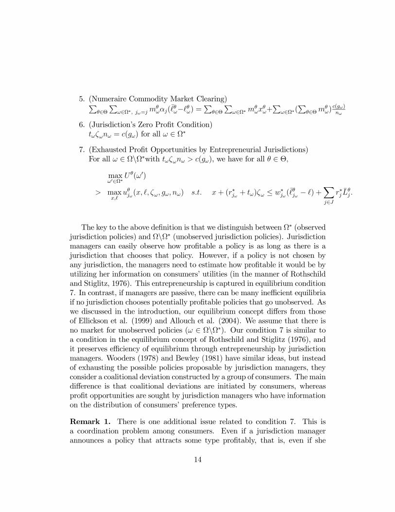
7. (Exhausted Profit Opportunities by Entrepreneurial Jurisdictions)For all ω ∈ Ω\Ω∗with tωζωnω > c(gω), we have for all θ ∈ Θ,

maxω0∈Ω∗

Uθ(ω0)

> maxx,

uθjω(x, , ζω, gω, nω) s.t. x+ (r∗jω + tω)ζω ≤ w∗jω(θjω − ) +

Xj∈J

r∗j Lθj .

The key to the above definition is that we distinguish between Ω∗ (observedjurisdiction policies) and Ω\Ω∗ (unobserved jurisdiction policies). Jurisdictionmanagers can easily observe how profitable a policy is as long as there is ajurisdiction that chooses that policy. However, if a policy is not chosen byany jurisdiction, the managers need to estimate how profitable it would be byutilizing her information on consumers’ utilities (in the manner of Rothschildand Stiglitz, 1976). This entrepreneurship is captured in equilibrium condition7. In contrast, if managers are passive, there can be many inefficient equilibriaif no jurisdiction chooses potentially profitable policies that go unobserved. Aswe discussed in the introduction, our equilibrium concept differs from thoseof Ellickson et al. (1999) and Allouch et al. (2004). We assume that there isno market for unobserved policies (ω ∈ Ω\Ω∗). Our condition 7 is similar toa condition in the equilibrium concept of Rothschild and Stiglitz (1976), andit preserves efficiency of equilibrium through entrepreneurship by jurisdictionmanagers. Wooders (1978) and Bewley (1981) have similar ideas, but insteadof exhausting the possible policies proposable by jurisdiction managers, theyconsider a coalitional deviation constructed by a group of consumers. The maindifference is that coalitional deviations are initiated by consumers, whereasprofit opportunities are sought by jurisdiction managers who have informationon the distribution of consumers’ preference types.

Remark 1. There is one additional issue related to condition 7. This isa coordination problem among consumers. Even if a jurisdiction managerannounces a policy that attracts some type profitably, that is, even if she

14

announces ω = (jω, gω, tω, ζω, nω) /∈ Ω∗ with tωζωnω > c(gω) such that forsome θ ∈ Θ,

maxω0∈Ω∗

U θ(ω0) (*)

< maxx,

uθjω(x, , ζω, gω, nω) s.t. x+ (r∗jω + tω)ζω ≤ w∗jω(θj − ) +

Xj∈J

r∗j Lθj

holds, a coordination problem may still arise. This problem occurs if consumersdo not like to have vacant houses in a jurisdiction. That is, if for all suchω /∈ Ω∗, there is n < nω (namely n = 1) such that for all θ ∈ Θ,

maxω0∈Ω∗

U θ(ω0) (**)

> maxx,

uθjω(x, , ζω, gω, n) s.t. x+ (r∗jω + tω)ζω ≤ w∗jω(θj − ) +

Xj∈J

r∗j Lθj

holds, then a pessimistic manager may have troubles in filling the new juris-diction with consumers. Consumers may believe that the jurisdiction wouldnever filled, and that they could be worse off if they move in. If this is the case,jurisdiction managers cannot feel safe to announce ω, although if type θ con-sumers would fill all vacancies, then both the consumers and the jurisdictionmanager would be strictly better off.22 If such pessimism by consumers andjurisdiction managers were allowed, condition 7 should be modified as follows:

7’. For all ω ∈ Ω\Ω∗with tωζωnω > c(gω), we have for all θ ∈ Θ, there existsn ∈ 1, ..., nω such that the above (**) holds.

However, then, our equilibrium concept would support inefficient alloca-tions. The following negative population externalities assumption eliminatessuch pessimism, and guarantees the efficiency of the Tiebout equilibrium withentrepreneurial jurisdictions. A simple way to avoid this coordination problemis to assume negative population externalities (NPE):

NPE. For all (θ, j, g) ∈ Θ × J × G, all (x, , z) ∈ R++ × [0, θj ] × R+ and all

n, n0 ∈ Z++ with n < n0, we have

uθj(x, , z, g, n) ≥ uθj(x, , z, g, n0).

22I thank Atsushi Kajii and one of the referees for raising this issue.

15

This condition is commonly assumed in local public goods economies, andasserts that consumers weakly prefer less crowded jurisdiction if all other thingsare equal. It assures that condition 7’ and NPE together imply condition 7of the Tiebout equilibrium with entrepreneurial jurisdictions, since the abovecoordination problem disappears.¥

The main result is stated below.

Theorem. There exists a Tiebout equilibrium with entrepreneurial jurisdic-tions, and it is Pareto efficient under the following assumptions about utilityfunctions:

1. For all θ ∈ Θ, all j ∈ J , all g ∈ G, all n ∈ N = 1, ..., n, , uθj(x, , L, g, n)is continuous and strictly monotonic in (x, , L),

2. for all θ ∈ Θ, all j ∈ J , all j ∈ [0, θj ], all L ∈ R+, all g ∈ G, all n ∈

N = 1, ..., n, uθj(0, , L, g, n) = uθ ≡ min(j0,x0, 0,L0,g0,n0) uθj0(0, 0, L0, g0, n0)(essentiality of numeraire),23

3. for all θ ∈ Θ, all j ∈ J , all g ∈ G, and all n ∈ N = 1, ..., n,uθj(x, , L, g, n) is strictly quasi-concave in (x, , L).

4 Sketch of the Proof

The formal proof is delegated to the appendix; here we give a sketch of theproof and remark on some of its key arguments. We prove the theorem withfour propositions. We first define “Tiebout equilibrium with poll taxes” andshow that it exists and is efficient (Propositions 1 and 2). Then we showthat this equilibrium is essentially equivalent to a Tiebout equilibrium withentrepreneurial jurisdictions (Propositions 3 and 4).With poll taxes, the definition of a policy is different. Let each jurisdic-

tion charge a poll tax τ = c(g)/n for a policy ω = (jω, gω, τ ω, nω) ∈ Ω =J × G × R+ × 1, ..., n. Besides this, a Tiebout equilibrium with poll taxesstill differ from a Tiebout equilibrium with entrepreneurial jurisdictions in

23See Mas-Colell (1977), Wooders (1978), and Ellickson (1979) for the spirit of this as-sumption.

16

two ways. First, jurisdictions’ tax policies are poll taxes instead of propertytaxes. Second, we assume a complete price system (there are prices for allω ∈ Ω) and no zoning restrictions. Our proof of the theorem is indirect:We analyze the properties of an equilibrium with poll taxes, and show thatthe equilibrium allocations are essentially equivalent between these two equi-librium concepts. A Tiebout equilibrium with poll taxes is easier to dealwith. Note that the jurisdiction policy space is now different (Ω instead of Ω:ω = (jω, gω, tω, ζω, nω) ∈ Ω).

Definition. A Tiebout equilibrium with poll taxes is a list of((r∗j , w

∗j )j∈J , (jω, gω, τ ω, nω)ω∈Ω, (m

θω, x

θω,

θω, z

θω)θ∈Θ,ω∈Ω) with

Pω∈Ωm

θω = mθ

for all θ ∈ Θ such that

1. (Optimality of Private Consumption Choice)For all ω ∈ Ω, and all θ ∈ Θ, 24 (xθω,

θω, z

θω) ∈ argmaxx, ,z uθjω(x, , z, gω, nω)

s.t. x + r∗jωz + τ ω ≤ w∗jω(θjω− ) +

Pr∗j L

θj , and if the budget set is

empty for θ, assign (0, 0, 0).25

2. (Optimality of Jurisdiction Choice)For all ω ∈ Ω, and all θ ∈ Θ with mθ

ω > 0, we haveω ∈ argmaxω0∈Ω Uθ(ω0; (r∗j , w

∗j )j∈J) = uθjω(x

θω,

θω, z

θω, gω, nω)

3. (Land Market Clearing)Pθ∈Θ

Pω∈Ω, jω=j m

θωzω ≤ Lj (with rj = 0 if inequality is strict) for all

j ∈ J

4. (Profit Maximization)w∗j =

1αjfor all j ∈ J

5. (Numeraire Commodity Market Clearing)Pθ∈Θ

Pω∈Ω, jω=j m

θωαj(

θω− θ

ω) =P

θ∈ΘP

ω∈Ωmθωx

θω+P

ω∈Ω(P

θ∈Θmθω)

c(gω)nω

24Note that not all types live in type ω jurisdictions. For some type θ, mθω = 0 may be

the case. For such a type, (xθω,θω, z

θω) is irrelevant information. However, for convenience,

we include these consumers’ optimal choices in the definition of equilibrium.25This is just for technical convenience (type θ consumers at ω has a zero measure). Under

assumption 2 in the theorem, (0, 0, 0) would not be a consumer’s choice (see the proof ofProposition 1). Also, we assign (xθω,

θω, z

θω) to type θ consumer at ω as long as the budget

set is nonempty even if mθω = 0. This is just for the purpose of obtaining a well-defined and

well-behaved fixed point mapping.

17

6. (Jurisdiction’s Zero Profit Condition)τ ωnω = c(gω) for all ω ∈ Ω.

Assuming a complete price system, that is, assuming there are prices forall possible ωs, we can find an equilibrium.26

Proposition 1. There exists a Tiebout equilibrium with poll taxes under thefollowing assumptions:

1. For all θ ∈ Θ, all j ∈ J , all g ∈ G, all n ∈ N = 1, ..., n, , uθj(x, , L, g, n)is continuous and strictly monotonic in (x, , L);

2. For all θ ∈ Θ, all j ∈ J , all j ∈ [0, θj ], all L ∈ R+, all g ∈ G, all

n ∈ 1, ..., n, uθj(0, , L, g, n) = uθ (essentiality of numeraire); and

3. For all θ ∈ Θ, all j ∈ J , all g ∈ G, and all n = N ∈ 1, ..., n,uθj(x, , L, g, n) is strictly quasi-concave in (x, , L).

The proof of Proposition 1 is basically along the lines of Ellickson et al.(1999), although ours is less technically involved since we use the distributionapproach (see Hart, Hildenbrand, and Kohlberg 1974) and assume strictlyquasi-concave utility. However, adding spatiality to the model complicates theproblem. First of all, we need to formalize the consumption sets of consumers.The difficulty is that each consumer’s leisure (labor) endowment/consumptionand land consumption are dependent on and restricted by her location choice.That is, if a consumer chooses a type ω jurisdiction at location jω ∈ J , herleisure endowment and her leisure and land consumption must be at locationjω. In contrast, land endowment is not affected by location choice. Further,gω ∈ G and nω ∈ 1, ..., n can affect consumers’ choices over private goodsconsumption. Under a complete market system, each consumer can chooseany ω ∈ Ω. These issues are illustrated in the following formalization of theconsumer’s choice problem.

26Since we need to accommodate zoning aspects in the end, it is hard to dispense withfinite types of consumers. Given the finiteness of Θ, we can use Konishi’s (1996) simplefixed point mapping.

18

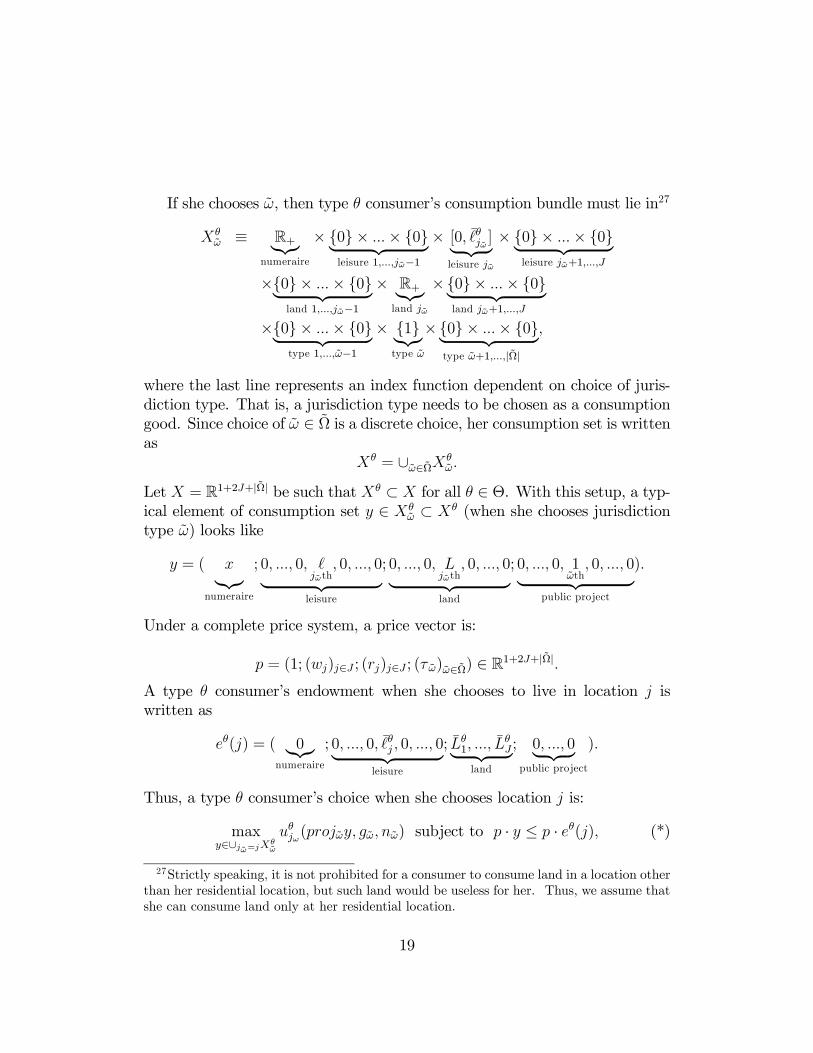
If she chooses ω, then type θ consumer’s consumption bundle must lie in27

Xθω ≡ R+|z

numeraire

× 0 × ...× 0| z leisure 1,...,jω−1

× [0, θjω]| z

leisure jω

× 0 × ...× 0| z leisure jω+1,...,J

×0 × ...× 0| z land 1,...,jω−1

× R+|zland jω

×0 × ...× 0| z land jω+1,...,J

×0 × ...× 0| z type 1,...,ω−1

× 1|ztype ω

×0 × ...× 0| z type ω+1,...,|Ω|

,

where the last line represents an index function dependent on choice of juris-diction type. That is, a jurisdiction type needs to be chosen as a consumptiongood. Since choice of ω ∈ Ω is a discrete choice, her consumption set is writtenas

Xθ = ∪ω∈ΩXθω.

Let X = R1+2J+|Ω| be such that Xθ ⊂ X for all θ ∈ Θ. With this setup, a typ-ical element of consumption set y ∈ Xθ

ω ⊂ Xθ (when she chooses jurisdictiontype ω) looks like

y = ( x|znumeraire

; 0, ..., 0,jωth

, 0, ..., 0| z leisure

; 0, ..., 0, Ljωth

, 0, ..., 0| z land

; 0, ..., 0, 1ωth

, 0, ..., 0| z public project

).

Under a complete price system, a price vector is:

p = (1; (wj)j∈J ; (rj)j∈J ; (τ ω)ω∈Ω) ∈ R1+2J+|Ω|.A type θ consumer’s endowment when she chooses to live in location j iswritten as

eθ(j) = ( 0|znumeraire

; 0, ..., 0, θj , 0, ..., 0| z

leisure

; Lθ1, ..., L

θJ| z

land

; 0, ..., 0| z public project

).

Thus, a type θ consumer’s choice when she chooses location j is:

maxy∈∪jω=jX

θω

uθjω(projωy, gω, nω) subject to p · y ≤ p · eθ(j), (*)

27Strictly speaking, it is not prohibited for a consumer to consume land in a location otherthan her residential location, but such land would be useless for her. Thus, we assume thatshe can consume land only at her residential location.

19

where projωy = (proj0y, proj jωy, projLjωy) = (x, , L).

One problemwhich arises in spatial models is that the value of a consumer’sendowment depends on her location choice (see (∗) above). This does not arisein defining the consumer’s choice problem, since she can compare the level ofindirect utility at each location j ∈ J , and choose a location that attainsthe highest indirect utility. Thus, we can prove Proposition 1 in this setup.However, it does pose a problem for proving the efficiency of the equilibrium.The standard proof of the first welfare theorem relies on comparisons of valuesof consumption bundles/endowments. It is essential for the proof to have thesame endowment values independent of consumers’ location choices.It turns out that this problem is not severe. We need only normalize the

consumer’s endowment to the origin so that the value of the endowment isalways zero irrespective of her location choice. A consumption set with sucha translation of the origin is called a trading set (McKenzie 1959). Once thistranslation is done, the standard argument proves the first welfare theorem.28

When a type θ consumer chooses ω, then her trading set is

Xθω ≡ R+|z

numeraire

× 0 × ...× 0| z leisure 1,...,jω−1

× [− θjω, 0]| z

leisure jω

× 0 × ...× 0| z leisure jω+1,...,J

×−Lθ1 × ...× −Lθ

jω−1| z land 1,...,jω−1

× [−Lθjω,∞)| z

land jω

×−Lθjω+1

× ...× −LθJ| z

land jω+1,...,J

×0 × ...× 0| z type 1,...,ω−1

× 1|ztype ω

×0 × ...× 0| z type ω+1,...,|Ω|

.

Since the choice of ω ∈ Ω is discrete, her trading set is written as

Xθ = ∪ω∈ΩXθω.

The utility function uθω : Xθω → R is also translated to uθω : X

θω → R accord-

ingly.

Proposition 2. Every Tiebout equilibrium with poll taxes is Pareto efficient.

Next, we transform the poll taxes to pairs of policies: property taxes andzoning policies. First, note that for each Tiebout equilibrium with poll taxes,

28See Berliant and Konishi (2000). Note that the trading set approach is effective in ajob choice model as well.

20

we can construct another sorting Tiebout equilibrium with poll taxes: that is,in each jurisdiction there is only one type of consumer for almost all jurisdic-tions. This step is needed, since in a Tiebout equilibrium with poll taxes, twodifferent types of consumers may choose the same ω. If this were the case,then in an equilibrium allocation these two different types may live togetherin the same jurisdiction while choosing two different amounts of land. Obvi-ously, a zoning policy cannot support such an allocation. For a zoning policyto work, we need perfect homogeneity in demand for land in each jurisdiction.To achieve perfect homogeneity, we need LP and FP. Under these assumptions,it is easy to see that there is always an equilibrium allocation in which eachjurisdiction has a perfectly homogeneous population. If in a Tiebout equilib-rium with poll taxes, mθ

ω > 0 and mθ0ω > 0 hold, then we can let measure

mθω/nω type ω jurisdictions have only type θ residents and measure m

θ0ω /nω

type ω jurisdictions have only type θ0 residents. We call such an equilibriumallocation a sorting Tiebout equilibrium allocation with poll taxes.29

Now we can construct the zoning policies. For each ω ∈ Ω∗, there is at least aθ ∈ Θ with mθ

ω > 0. For them, we construct ω: i.e., a zoning policy ζω = zθωwith tω = τ ω = c(gω)/nωζω. This works as a Hamilton zoning policy. Thefollowing two propositions establish the essential equivalence between Tieboutequilibrium with entrepreneurial jurisdictions and Tiebout equilibrium withpoll taxes.

Proposition 3. Every sorting Tiebout equilibrium allocation with poll taxescan be supported by a Tiebout equilibrium with entrepreneurial jurisdictions.

Proposition 4. Every Tiebout equilibrium allocation with entrepreneurialjurisdictions can be supported by a sorting Tiebout equilibrium allocationwith poll taxes.

These propositions clarify how the equilibrium concept of Rothschild andStiglitz (1976) achieves efficient allocations: all types of consumers can achievethe highest possible utility under segregation. This key observation is summa-rized formally as follows.

29Strictly speaking, it may not be necessary to introduce different jurisdictions for alltypes. As Hamilton (1975) correctly points out, as long as two types θ and θ0 consume thesame amount of land at ω, zoning policies can support mixed jurisdictions by these types.

21

Observation. In all Tiebout equilibria with entrepreneurial jurisdictions,Uθ(ω; (r∗j , w

∗j )j∈J) = maxω0∈Ω:tωζωnω≥c(gω) U

θ(ω0; (r∗j , w∗j )j∈J) for all θ ∈ Θ and

all ω ∈ Ω∗ with mθω > 0.

That is, if type θ consumers choose jurisdiction type ω in the equilibrium,then their utility levels are the highest among all possible (including nonexist-ing) jurisdiction types that satisfy budget-balancing conditions. This is howour Tiebout equilibrium with entrepreneurial jurisdictions achieves efficiencythrough managers’ entrepreneurship and consumers’ self-selection given fis-cally anonymous congestion.

5 Concluding Remarks

We can relax the conditions in the Theorem quite a bit. We actually do notneed quasi-concavity of utility functions (convexity of preferences). We as-sumed convexity only for simplicity. Our theorem can be easily extended toa more general setting with many private goods, general (CRS) productiontechnologies, and many different occupations. Conley and Wooders (1996)consider occupation choice with an occupation-dependent crowding type, andshow that the equilibrium is efficient if an occupation-dependent nonanony-mous tax can be imposed. In contrast, since we do not assume that crowdingis type-dependent, if we just allow that utility and wage depend on occupa-tion choice then such occupation-dependent taxes are not necessary to attainefficiency.Note that our theorem holds only in an idealized situation, since it requires

that there be very many jurisdictions for each location, which is not veryrealistic. If there are limited numbers of jurisdictions in each location, thentwo problems can occur: monopoly powers by jurisdictions, and insufficientchoice sets provided by jurisdictions. Allowing free entry of new jurisdictionsmay sound reasonable in our setup, since it includes large numbers of negligiblysmall jurisdictions. However, in reality, unless there is unused land (or farmland or forest) in equilibrium,30 the implicit assumption of free entry does notseem easily justifiable. At least, the locations near central business districtsshould not have plenty of unused land. Moreover, the model is static, soour theorem does not touch on how to rearrange jurisdiction borders when a

30Bewley (1981) and Bruckner (1981) have discussions on this matter.

22

new jurisdiction is set up, or on how to ask current residents to move from anexisting jurisdiction that is not profitable.31 Thus, there is more friction in thepresence of a spatial structure, and Tiebout’s tale becomes harder to justify.Despite the above cautious remark, our theorem may find another useful

application in urban economic theory. We can apply directly our theoremto prove the existence and efficiency of a closed-economy monocentric cityequilibrium with transport costs (in commuting time) when housing quality isendogenous as long as there is a finite number of rings of heterogeneous land(distinguished by the distance from the CBD).32 Houses and condo buildingsare easier to demolish and rebuild than jurisdictions, so it might be easier tojustify the free entry assumption in this case. In monocentric city models,housing and land are used almost interchangeably. However, in our model, ifwe interpret g as a housing quality, we can let consumers choose their ownhousing qualities. Since multiple people can share the same g, we can dealwith collective residential buildings (condos/apartments instead of houses).More formally, let us order locations j0, j1, ..., jK , and assume that productioncan be made only in the CBD location j0: i.e., αj = ∞ for j 6= j0, whileαj0 < ∞. As index k increases, the distance from the CBD increases. As aresult, for all θ ∈ Θ, θ

j0> θ

j1> ... > θ

jK(commuting time difference). If

the geography is one-dimensional (as in a linear city), then we may assumeLjk = Ljk0 for all k, k

0 ∈ 0, 1, ...,K. If it is two-dimensional, then we mayassume Lj0 < Lj1 < ... < LjK . We interpret ω = (gω, nω) ∈ Ω as a buildingthat can be a house or a condo/apartment: gω is a type of building (say,high quality, low quality, with a swimming pool, or with a nicely landscapedgarden, etc.) and nω is the number of households living in the building (ifnω = 1 then it is a single household house, and if nω is large it is an apartmentcomplex). Our theorem says that there is an equilibrium sorting with varioushousing qualities including collective housing such as apartments.33 Assuming

31Berliant (1985) analyzes a formulation of parcel land market (say, total land endowmentin an economy is a two-dimensional set, and each consumer consumes a subset of it withoutoverlapping with other consumers’ land consumption). He proves that a continuum economy(continuum of consumers) is inconsistent with parcel land market. Berliant and Fujita (1992)look at equilibrium in a spatial economy with parcel land and finite population. We avoiddifficulties by assuming a quantity of land instead (the total land endowment of an economyis a quantity of land vector at all locations).32See Fujita (1989) for many kinds of monocentric city models.33Finiteness of locations may be dropped by applying the method by LaFountain (2006).

In order to show efficiency of equilibrium, we need to assume that there are no congestion

23

that land at each location is physically the same and that land is a normalgood, it is easy to see that land prices go down as index k increases, sincechoosing a smaller index location means more (potential) income for all θ ∈Θ. However, other characteristics of equilibrium allocations require furtherassumptions about consumers’ preferences over Ω and the distributions of theirland endowments.34

Actually, the "monocentric" assumption is not important for the existenceand efficiency results. Even if a consumer can freely choose her locations ofresidence and work, our results are not affected. The only modification neededis to assume that each consumer (say type θ) chooses a pair of locations: herresidential location and working location, (j, j0) ∈ J × J , and her leisureendowment for the choice is θ

jj0 since her commuting time depends on herresidential and work locations (see the concluding remarks in Konishi 1996).

Appendix

Here we collect all proofs of Propositions.

Proposition 1. There exists a Tiebout equilibrium with poll taxes under thefollowing assumptions:

1. For all θ ∈ Θ, all j ∈ J , all g ∈ G, all n ∈ N = 1, ..., n, , uθj(x, , L, g, n)is continuous and strictly monotonic in (x, , L);

2. for all θ ∈ Θ, all j ∈ J , all j ∈ [0, θj ], all L ∈ R+, all g ∈ G, all

n ∈ 1, ..., n, uθj(0, , L, g, n) = uθ (essentiality of numeraire); and

3. for all θ ∈ Θ, all j ∈ J , all g ∈ G, and all n = N ∈ 1, ..., n,uθj(x, , L, g, n) is strictly quasi-concave in (x, , L).

Proof of Proposition 1. Although we normalized the numeraire price atunity in the set up, we actually need to have a compact price set. So it is moreconvenient for us to use a J + 1 dimensional price simplex ∆ ≡ p ∈ RJ+1

+ :

externalities in commuting.34It may be interesting to analyze the relationship between housing quality and distance

from the CBD.

24

PJj=0 pj = 1 (numeraire and land prices, where p0 and pj (j 6= 0) represent the

numeraire price and land price at location j,35 respectively: wages and publicproject prices are tied up with the numeraire price by assumption36) We needto show that the relative price of the numeraire does not go to zero as well, butthis is easily shown by considering a sequence of -truncated price simplices∆( ) ≡ p ∈ RJ+1

+ :PJ

j=0 pj = 1 and pj ≥ ( < 1J+1), and taking the limit

of a sequence of -equilibria (equilibria within -truncated price simplex) asapproaches zero (with assumption 1). For simplicity, we omit this procedure.37

With an abuse of notation, we let ∆ = ∆( ).To make each consumer’s consumption set compact, we truncate consump-

tion sets by placing an upper bound on the numeraire and land consumption,and we take a sequence of equilibria for increasing upper bounds.38 The limitwill be shown to be an equilibrium allocation (see, e.g., Hildenbrand 1972).For each θ and ω, let Xθ

ω(k) be such that

Xθω(k) ≡ Xθ

ω ∩ [0, k]1+2J+|Ω|

and let Xθ(k) = ∪ω∈ΩXθω(k), where k = 1, 2, .... Obviously, for each k, Xθ(k)

is a compact set.For each θ ∈ Θ, let βθω : ∆³ Xθ

ω(k) be type θ’s budget correspondence atω ∈ Ω such that39

βθω(p) = (x, , z) ∈ projωXθω(k) : p0x+ pjωz+τ ω ≤

p0αjω

( θjω− )+

Xpjω0 L

θjω0,

where τ ω = p0c(gω)/nω (condition 6). Although βθkω is compact-valued, it canbe empty-valued for some ps due to a poll tax τ ω. Under such ps, type θ

35Thus, rj = pj/p0.36It is easy to endogenize wages and public project prices using flexible production tech-

nologies.37The procedure of taking a limit is routine (for a spatial economy, see Konishi 1996,

Lemma 3). Basically, the result holds by upper hemicontinuity of best response correspon-dences.38If the number of consumers if finite, we do not need this procedure: each consumer’s

feasible consumption plan is bounded. However, in an atomless economy, each consumer’sfeasible consumption set is unbounded since the measure of consumers who live in a locationcan be very small, which in turn means that each consumer’s consumption plan in such alocation can be very large. This is why we need to take the limit of an equilibrium sequence.39Although correspondence βθω is dependent on k, we omit k to simplify the notation.

The same comment applies to δθω, Uθ and others.

25

consumer cannot live in jurisdiction ω. In order to overcome this emptinessproblem, let ∆θ

ω ≡ p ∈ ∆ : τ ω < p0αjω( θ

j − ) +P

pjω0 Lθjω0 be the set of price

vectors in which type θ consumer’s budget set at ω has a cheaper point. Notethat ∆θ

ω is open relative to ∆. Let δθω : ∆θω ³ R+ × [0, θ

j ] × R+ be type θ’sdemand correspondence when she is forced to choose ω ∈ Ω such that

δθω(p) = (x, , z) ∈ βθω(p) : uθjω(x, , z, gω, nω) ≥ uθjω(x

0, 0, z0, gω, nω) ∀(x0, 0, z0) ∈ βθω(p).

By Weierstrass’s theorem and Berge’s maximum theorem, δθω is nonempty-valued and upper hemicontinuous. Moreover, strict quasi-concavity guaranteessingle-valuedness. That is, δθω is a continuous function.Now, we will move toward consumers’ jurisdiction choice mapping. One

obstacle we need to overcome is how to extend the domain of the above de-mand correspondence to ∆ without affecting the consumers’ actual choicecorrespondence. Let δθω : ∆→ Xθ

ω(k) be such that

δθω(p) =

½δθω(p) if p ∈ ∆θ

ω,0 if p /∈ ∆θ

ω.

This is again a continuous function.40 Note that Assumption 2 says thattype θ consumers get uθ in the latter case. For each p ∈ ∆θ

ω, let Uθ(ω; p) ≡

uθjω(δθω(p)). This is a continuous function. Now, we can construct type θ

consumer’s jurisdiction choice mapping. Let λθ : ∆³ Ω be such that λθ(p) =ω ∈ Ω : U θ(ω; p) = max Uθ(ω0; p). By Berge’s maximum theorem, λθ isan upper hemicontinuous correspondence. Since we allow ∅ ∈ G (no publicproject) with c(∅) = 0, as long as the price of the numeraire is positive, thereis an ω ∈ Ω with ∆θ

ω = ∆ for gω = ∅ (denote ω∅). Thus, for all p ∈ ∆, andall θ ∈ Θ, for ω∅ ∈ Ω there is a cheaper point in her budget constraint. Thus,Uθ(ω∅; p) > uθ for all p ∈ ∆ by Assumptions 1 and 2. This assures that forall price vectors p ∈ ∆, each type θ obtains a utility strictly higher than uθ,which makes type θ consumers’ choices under p /∈ ∆θ

ω (and extension parts ofδθω) irrelevant. That is, if ω ∈ λθ(p) then p ∈ ∆θ

ω. Since type θ consumers areindifferent among λθ(p), their optimal location choices generate a populationdistribution defined by the following population mapping: μθ : ∆ ³ Mθ,where Mθ = (mθ

ω)ω∈Ω ∈ RΩ+ :P

ω∈Ωmθω = mθ, such that

μθ(p) = (mθω)ω∈Ω ∈Mθ : mθ

ω > 0 only if ω ∈ λθ(p).40As long as the price vector is positive, the budget constraint at ω shrinks to the origin

around the boundary of ∆θω, so δ

θω is a continuous function.

26

It is easy to see that μθ is upper hemicontinuous and convex-valued. Letμ : ∆³ Πθ∈ΘM

θ be such that μ(p) ≡ Πθ∈Θμθ(p) for all p ∈ ∆.

Next, we move on to excess demand correspondence (in the numeraire andland markets). First, let the feasible excess demand set under the populationdistribution m = (mθ

ω)θ∈Θ,ω∈Ω ∈ Πθ∈ΘMθ be:

F (m) ≡©(f0, f1, ..., fJ) ∈ R×RJ :

f0 =X

θ∈Θ,ω∈Ω

mθωx

θω −

Xj∈J

1

αj×Xθ∈Θ

Xω∈Ω,jω=j

mθω(

θj − θ

j)−Xω∈Ω

Xθ∈Θ

mθω ×

c(gω)

nω,

and fj =Xθ∈Θ

Xω∈Ω,jω=j

mθωz

θω − Lj for all j ∈ J

for a vector (xθω,θω, z

θω)θ∈Θ,ω∈Ω that is consistent with Xθ

ω(k) for all θ and ωª.

Let F ≡ co(∪m∈Πθ∈ΘMθF (m)), where co(·) denotes a convex hull of ·. Forexcess demand correspondence: Let ψ :

Qθ∈Θ,ω∈ΩX

θω(k) ×

Qθ∈ΘM

θ → F besuch that

ψ0((xθω,

θω, z

θω,m

θω)θ∈Θ,ω∈Ω)

=X

θ∈Θ,ω∈Ω

mθωx

θω −

Xj∈J

1

αj×Xθ∈Θ

Xω∈Ω,jω=j

mθω(

θj − θ

j)−Xω∈Ω

Xθ∈Θ

mθω ×

c(gω)

nω,

and

ψj((xθω,

θω, z

θω,m

θω)θ∈Θ,ω∈Ω)

=Xθ∈Θ

Xω∈Ω,jω=j

mθωz

θω − Lj for all j ∈ J.

It is clear that ψ is a continuous function. Finally, we define a price mappingbased on Gale-Nikaido’s lemma. Let π : F ³ ∆ be such that

π(f) = p ∈ ∆ : p · f ≥ p0 · f for all p0 ∈ ∆.

It is clear that π is nonempty-valued, upper hemicontinuous, and convex-valued.Our fixed point mapping is

ξ : ∆×Y

θ∈Θ,ω∈ΩXθ

ω(k)×Y

θ∈ΘMθ×F ³ ∆×

Yθ∈Θ,ω∈Ω

Xθω(k)×

Yθ∈Θ

Mθ×F

27

which is a Cartesian product of

π : F ³ ∆,

δ : ∆³Y

θ∈Θ,ω∈ΩXθ

ω(k),

μ : ∆³Y

θ∈ΘMθ,

ψ :Y

θ∈Θ,ω∈ΩXθ

ω(k)×Y

θ∈ΘMθ ³ F .

By construction, we know that ∆, Xθω(k), M

θ and F are nonempty, compact,convex sets, and from our analysis, we also know that π, δ, μ and ψ are allnonempty-valued, upper hemicontinuous, and convex-valued correspondences.Since a product of upper hemicontinuous correspondences is upper hemicon-tinuous,41 the fixed point mapping is upper hemicontinuous. Thus, we canapply the Kakutani fixed point theorem, and there exists a fixed point

(p, (xθω,θω, z

θω,m

θω)θ∈Θ,ω∈Ω, f) ∈ ξ(p, (xθω,

θω, z

θω,m

θω)θ∈Θ,ω∈Ω, f).

The Gale-Nikaido’s lemma (see Debreu 1959) proves the clearance of markets(conditions 3 and 5 with inequalities: 4 is already built in). Conditions 1 and2 follow from the constructions of δ and μ. Condition 6 has been built in tothe analysis. Thus, all conditions hold assuming that xθω ∈ Xθ

ω(k) is indeedthe optimal choice (at ω) for nontruncated consumption set Xθ

ω. But this as-sumption does not necessarily hold. Thus, we take k to infinity, and constructa sequence of fixed points of ξ. In the space of aggregated consumption, thissequence converges, and we can find an equilibrium (see Konishi 1996). Fi-nally, we take to zero, and show that in equilibrium the numeraire has apositive price (p0 > 0) and thus, we can use another normalization p0 = 1 asis done in the main text.42¥

Proposition 2. Every Tiebout equilibrium with poll taxes is Pareto efficient.

Proof of Proposition 2. We will focus on “equal-treatment” allocationswithin the same type and the same location: that is, all consumers of the same

41A product of closed graphs is a closed graph.42At some locations, land price may become zero (measure zero consumers reside). Our

assumptions do not prevent this from happening. Assumption 2 does not exclude the fol-lowing situation: at a location, consumers’ utilities are bounded above (by unattractivenessof the location), and in equilibrium, nobody resides at the location despite free land.

28

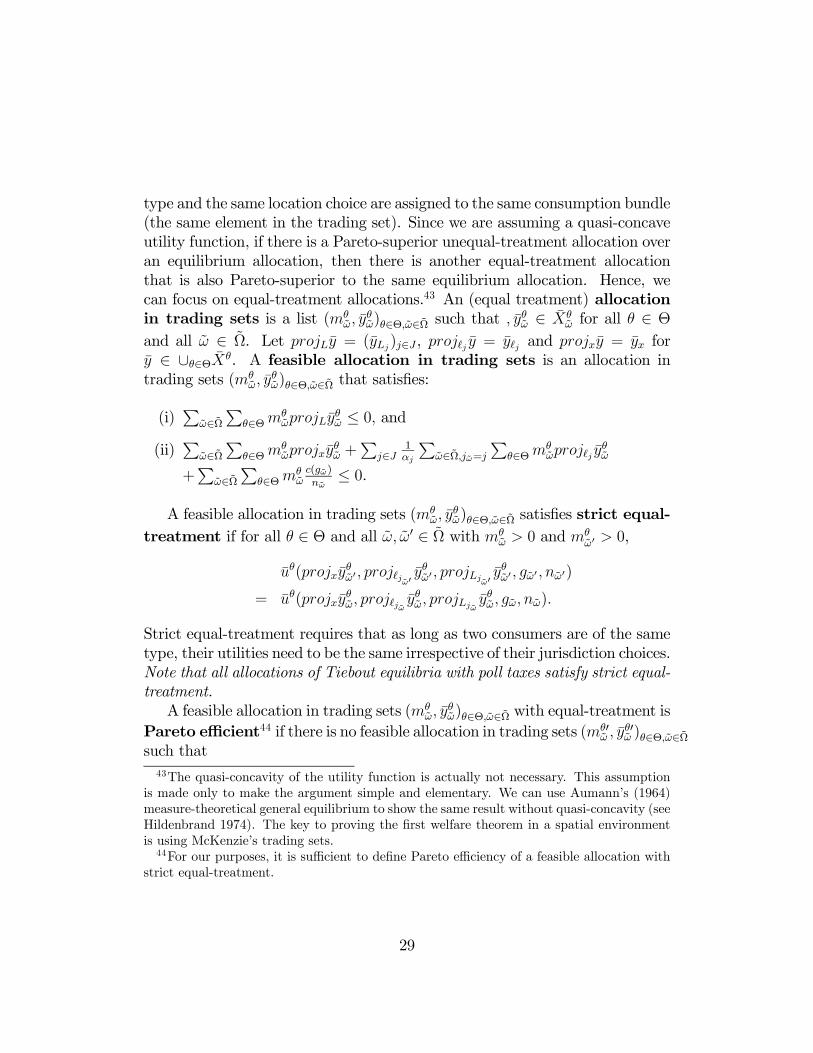
type and the same location choice are assigned to the same consumption bundle(the same element in the trading set). Since we are assuming a quasi-concaveutility function, if there is a Pareto-superior unequal-treatment allocation overan equilibrium allocation, then there is another equal-treatment allocationthat is also Pareto-superior to the same equilibrium allocation. Hence, wecan focus on equal-treatment allocations.43 An (equal treatment) allocationin trading sets is a list (mθ

ω, yθω)θ∈Θ,ω∈Ω such that , y

θω ∈ Xθ

ω for all θ ∈ Θ

and all ω ∈ Ω. Let projLy = (yLj)j∈J , proj j y = y j and projxy = yx fory ∈ ∪θ∈ΘXθ. A feasible allocation in trading sets is an allocation intrading sets (mθ

ω, yθω)θ∈Θ,ω∈Ω that satisfies:

(i)P

ω∈ΩP

θ∈ΘmθωprojLy

θω ≤ 0, and

(ii)P

ω∈ΩP

θ∈Θmθωprojxy

θω +

Pj∈J

1αj

Pω∈Ω,jω=j

Pθ∈Θm

θωproj j

yθω

+P

ω∈ΩP

θ∈Θmθωc(gω)nω≤ 0.

A feasible allocation in trading sets (mθω, y

θω)θ∈Θ,ω∈Ω satisfies strict equal-

treatment if for all θ ∈ Θ and all ω, ω0 ∈ Ω with mθω > 0 and mθ

ω0 > 0,

uθ(projxyθω0 , proj jω0

yθω0 , projLjω0 yθω0 , gω0 , nω0)

= uθ(projxyθω, proj jω

yθω, projLjω yθω, gω, nω).

Strict equal-treatment requires that as long as two consumers are of the sametype, their utilities need to be the same irrespective of their jurisdiction choices.Note that all allocations of Tiebout equilibria with poll taxes satisfy strict equal-treatment.A feasible allocation in trading sets (mθ

ω, yθω)θ∈Θ,ω∈Ω with equal-treatment is

Pareto efficient44 if there is no feasible allocation in trading sets (mθ0ω , y

θ0ω )θ∈Θ,ω∈Ω

such that43The quasi-concavity of the utility function is actually not necessary. This assumption

is made only to make the argument simple and elementary. We can use Aumann’s (1964)measure-theoretical general equilibrium to show the same result without quasi-concavity (seeHildenbrand 1974). The key to proving the first welfare theorem in a spatial environmentis using McKenzie’s trading sets.44For our purposes, it is sufficient to define Pareto efficiency of a feasible allocation with

strict equal-treatment.

29

(i) for all θ ∈ Θ, all ω, ω0 ∈ Ω with mθω > 0 and mθ0

ω0 > 0,

uθ(projxyθ0ω0 , proj jω0

yθ0ω0 , projLjω0 yθ0ω0 , gω0 , nω0)

≥ uθ(projxyθω, proj jω

yθω, projLjω yθω, gω, nω)

(ii) for some ω, ω0 ∈ Ω with mθω > 0 and mθ0

ω0 > 0,

uθ(projxyθ0ω0 , proj jω0

yθ0ω0 , projLjω0 yθ0ω0 , gω0 , nω0)

> uθ(projxyθω, proj jω

yθω, projLjω yθω, gω, nω).

By using the above representation in trading sets, a Tiebout equilibriumwith poll taxes can be represented in the following way. Let p ∈ R1+2J+|Ω|+ besuch that

p =

Ã1,

µ1

αj

¶j∈J

, (rj)j∈J ,

µc(gω)

nω

¶ω∈Ω

!.

Note that the definition of p includes zero profit conditions by jurisdictions, andprofit maximizing firms (Conditions 4 and 6). Feasibility requires Conditions3 and 5. Thus, what is left is utility maximization by consumers (Conditions1 and 2), and the following lemma is a straightforward consequence.

Lemma. A Tiebout equilibrium with poll taxes can be represented as a listof a price vector and a feasible allocation in trading sets (p∗, (mθ

ω, yθω)θ∈Θ,ω∈Ω)

such that yθω ∈ argmaxy∈βθω(p∗) uθω(projxy, proj jω

y, projLjωy, gω, nω) holds for

ω ∈ Ω with mθω > 0, where βθω(p

∗) = y ∈ Xθω : p

∗ · y ≤ 0.

With this representation, we can prove the first welfare theorem. Let(p∗, (mθ∗

ω , yθ∗ω )θ∈Θ,ω∈Ω) be a Tiebout equilibrium with poll taxes. Suppose that

there exists a feasible allocation in trading sets (mθ0ω , y

θ0ω )θ∈Θ,ω∈Ω such that

(i) for all θ ∈ Θ, all ω, ω0 ∈ Ω with mθ∗ω > 0 and mθ0

ω0 > 0,

uθ(projxyθ0ω0 , proj jω0

yθ0ω0 , projLjω0 yθ0ω0 , gω0 , nω0)

≥ uθ(projxyθ∗ω , proj jω

yθ∗ω , projLjω yθ∗ω , gω, nω);

and

30

(ii) for some ω, ω0 ∈ Ω with mθ∗ω > 0 and mθ0

ω0 > 0,

uθ(projxyθ0ω0 , proj jω0

yθ0ω0 , projLjω0 yθ0ω0 , gω0 , nω0)

> uθ(projxyθ∗ω , proj jω

yθ∗ω , projLjω yθ∗ω , gω, nω).

Since utility functions are monotonic, consumers’ budget constraints arebinding in utility maximization under a Tiebout equilibrium with poll taxes.Thus, by (i) p∗ · yθ0ω ≥ 0 for all θ ∈ Θ and all ω ∈ Ω with mθ0

ω > 0, and by (ii)p∗ · yθ0ω > 0 for all θ ∈ Θ and all ω ∈ Ω with mθ0

ω > 0. Thus, we haveXω∈Ω

Xθ∈Θ

mθ0ωprojxy

θ0ω +

Xj∈J

1

αj

Xω∈Ω,jω=j

Xθ∈Θ

mθ0ωproj j y

θ0ω

+Xω∈Ω

Xθ∈Θ

mθ0ω

c(gω)

nω+Xω∈Ω

Xθ∈Θ

mθ0ω

¡r · projLyθ0ω

¢> 0,

where r = (rj)j∈J . Since the price of the numeraire is positive, and all landprices are nonnegative, we have eitherXω∈Ω

Xθ∈Θ

mθ0ωprojxy

θ0ω +

Xj∈J

1

αj

Xω∈Ω,jω=j

Xθ∈Θ

mθ0ωproj j y

θ0ω +

Xω∈Ω

Xθ∈Θ

mθ0ω

c(gω)

nω> 0,

or Xω∈Ω,j=jω

Xθ∈Θ

mθ0ω rjprojLj y

θ0ω > 0 for some j ∈ J .

In the former case, there is excess demand for the numeraire, and in thelatter case, at least in one location there is excess demand for land. Thus,(mθ0

ω , yθ0ω )θ∈Θ,ω∈Ω is infeasible. This is a contradiction. Thus, (m

θ∗ω , y

θ∗ω )θ∈Θ,ω∈Ω

is Pareto optimal.¥

Proposition 3. Every sorting Tiebout equilibrium allocation with poll taxescan be supported by a Tiebout equilibrium with entrepreneurial jurisdictions.

Proof of Proposition 3. For each ω ∈ Ω and for each θ ∈ Θ, we willconstruct ω ∈ Ω. Let (jω, gω, nω) = (jω, gω, nω) and tω ≡ τ ω

nωzθω, and ζω ≡ zθω.

Collecting all these types of jurisdictions, we can construct set Ω. Let Ω∗ ≡

31

ω ∈ Ω : mθω > 0. First, it is easy to see that if a type θ consumer lives in

a type ω jurisdiction (constructed by ω and θ), then she chooses to consume(xθω,

θω, ζω) = (x

θω,

θω, z

θω). Her budget constraint under the zoning constraint

isx+ (r∗jω + tω)z ≤ w∗jω(

θj − ) +

Xr∗jω L

θjω and zω ≥ ζω,

and her budget constraint in the Tiebout equilibrium under poll taxes is

x+ r∗jωz + τ ω ≤ w∗jω(θj − ) +

Xr∗jω L

θjω.

Since land price is higher under property taxes, the budget constraint underzoning is a subset of the budget constraint under poll taxes (see Figure 2).Since her optimal choice under poll taxes is (xθω,

θω, z

θω) = (x

θω,

θω, ζω) under the

larger budget set, and since (xθω,θω, ζω) is available under the zoning constraint,

her optimal choice under the zoning constraint is (xθω,θω, ζω) as well.

45 Now,given this, it is easy to see that each type is optimizing her jurisdiction choice.What is left is condition 7. Suppose that there is a policy ω ∈ Ω\Ω∗with

tωζωnω > c(gω). Suppose that there is a type θ ∈ Θ,

maxω0∈Ω∗

Uθ(ω0)

≤ maxx,

uθjω(x, , ζω, gω, nω) s.t. x+ (r∗jω + tω)ζω ≤ w∗jω(θj − ) +

Xr∗jω L

θjω .

This implies that there exists τω = tωζω such that τωnω > c(gω) and

maxω0∈Ω∗

Uθ(ω0)

≤ maxx, ,z

uθjω(x, , z, gω, nω) s.t. x+ r∗jωz + τω ≤ w∗jω(θj − ) +

Xr∗jω L

θjω .

However, ω corresponds to one of ω ∈ Ω, and reducing τω improves con-sumers’ utility. Thus, this contradicts the optimality of jurisdiction choice inthe definition of Tiebout equilibrium with poll taxes.¥

Proposition 4. Every Tiebout equilibrium allocation with entrepreneurialjurisdictions can be supported by a sorting Tiebout equilibrium allocationwith poll taxes.

45Without zoning, she would have wanted to consume less land, but the zoning constraintdoes not allow this (see Figure 2).

32

Proof of Proposition 4. With (r∗j , w∗j )j∈J , and allocation for ω ∈ Ω∗ and θ

withmθω > 0, it is easy to construct the rest of the allocations (mθ

ω, xθω,

θω, z

θω)θ∈Θ,ω∈Ω

formθω = 0 (use condition 1 if the budget set is nonempty for θ in ω: otherwise,

assign (0, 0, 0)). We show that this allocation is a Tiebout equilibrium withpoll taxes.Suppose that condition 1 of the Tiebout equilibrium with poll taxes is

violated. Then, the same must be true for ω that corresponds to ω ∈ Ω∗ formθ

ω > 0. Let (x, , z) ∈ R+ × [0, θjω]×R+ be such that

uθjω(x, , z, gω, nω) > uθjω(xθω,

θω, z

θω, gω, nω) and x+r∗jωz+τ ω ≤ w∗jω(

θj− )+

Xr∗jω L

θjω.

This means that there exist τ 0 > τω and (x0, 0, z0) ∈ R+ × [0, θjω]× R+ with

(x0, 0, z0) = argmaxuθjω(x, , z, gω, nω) s.t. x0+r∗jωz

0+τ 0 ≤ w∗jω(θj− 0)+

Xr∗jω L

θjω

uθjω(x0, 0, z0, gω, nω) ≥ uθjω(x

θω,

θω, ζω, gω, nω).

Since τω = c(ω)/nω, by letting (jω0 , gω0 , tω0 , ζω0 , nω0) = (jω, gω,τωz0 , z

0, nω), weget

uθjω0 (x0, 0, ζω0 , gω0 , nω0) ≥ uθjω(x

θω,

θω, ζω, gω, nω),

andx0 + (r∗jω0 + tω0)ζω0 + τ 0 ≤ w∗jω(

θj − 0) +

Xr∗jω L

θjω.

This means that Condition 7 of the Tiebout equilibrium with entrepreneurialjurisdictions is violated, which is a contradiction. Thus, Condition 1 of theTiebout equilibrium with poll taxes is satisfied.Suppose that Condition 2 is violated. Then for some θ and some ω with

mθω > 0, there is a jurisdiction ω0 with mθ

ω = 0 (otherwise, Condition 2 of theTiebout equilibrium with entrepreneurial jurisdictions is violated) and

uθjω0 (xθω0 ,

θω0 , z

θω0 , gω0 , nω0) > uθjω(x

θω,

θω, z

θω, gω, nω).

However, if so, we can slightly raise τ 0 > τ ω and reduce the consumption vectorwithout altering the above inequality. Then, we can construct a property taxand zoning policy that mimic such an allocation. Thus, Condition 7 of theTiebout equilibriumwith entrepreneurial jurisdictions is violated, and we reacha contradiction again.Conditions 3, 4, 5, and 6 of the Tiebout equilibrium with poll taxes follow

directly.¥

33

Proof of Theorem. Propositions 1, 2, 3, and 4 together prove the statementof the theorem.¥

References

[1] Allouch, N., J.P. Conley and M.H. Wooders, The Tiebout Hypothesis: Onthe Existence of Pareto Efficient Competitive Equilibria, (2004), mimeo-graph.

[2] Aumann, R.J., Markets with a Continuum of Traders, Econometrica 32(1964), 39-50.

[3] Berliant, M., Equilibrium Models with Land: Criticisms and an Alterna-tive, Regional Science and Urban Economics 15, (1985), 325-340.

[4] Berliant, M., and M. Fujita, Alonso’s Discrete Population Model of LandUse: Efficient Allocation and Competitive Equilibria, International Eco-nomic Review 33, (1992), 535-566.

[5] Berliant, M. and H. Konishi, The Endogenous Formation of a City: Pop-ulation Agglomeration and Marketplaces in Location-Specific ProductionEconomy, Regional Science and Urban Economics 30, (2000), 289-324.

[6] Bewley, T. A Critique of Tiebout’s Theory of Local Public Expenditures,Econometrica 49, (1981), 713-740.

[7] Brueckner, J. K., Zoning and Property Taxation in a System of LocalGovernments: Further Analysis, Urban Studies 18, (1981), 113-120.

[8] Buchanan, J. and C. Goetz, Efficiency Limits of Fiscal Mobility: AnAssessment of the Tiebout Model, Journal of Public Economics 1, (1972),25-43.

[9] Buchanan, J., and R. Wagner, An Efficiency Basis for Federal FiscalEqualization, in “The Analysis of Public Output,” J. Margolis ed., NBER,New York, 1970.

34

[10] Conley, J.P., and M.H. Wooders, Taste-Homogeneity of Optimal Juris-dictions in a Tiebout Economy with Crowding Types and EndogenousEducational Investment Choices, Recherche Economiche 50, (1996), 367-387.

[11] Debreu, G., “Theory of Value,” Wiley, New York, 1959.

[12] Ellickson, B., Competitive Equilibrium with Local Public Goods, Journalof Economic Theory 21, (1979), 46-61.

[13] Ellickson, B., B. Grodal, S. Scotchmer, and W.R. Zame, Clubs and theMarket, Econometrica 67, (1999), 1185-1217.

[14] Flatters, F., V. Henderson, and P. Mieszkowski, Public Goods, Efficiency,and Regional Fiscal Equalization, Journal of Public Economics 3, (1974),99-112.

[15] Fujita, M.,“Urban Economic Theory - Land Use and City Size,” Cam-bridge University Press, 1989.

[16] Hamilton, B.W., Zoning and Property Taxation in a System of LocalGovernments, Urban Studies 12, (1975), 205-211.

[17] Hart, S., W. Hildenbrand and E. Kohlberg, On equilibrium allocationsas distributions on the commodity space, Journal of Mathematical Eco-nomics 1, (1974), 159-166.

[18] Henderson, J.V., The Sizes and Types of Cities, American Economic Re-view 64, (1974), 640-656.

[19] Hildenbrand, W., “Core and Equilibrium in a Large Economy,” PrincetonUniv. Press, NJ, 1974.

[20] Ichiishi, T., “Game Theory for Economic Analysis,” Academic Press, NewYork, 1983.

[21] Kaneko, M., and M.H. Wooders, The Core of a Game with a Continuumof Players and Finite Coalitions: The Model and Some Results, Mathe-matical Social Sciences 12, (1986), 105-137.

35

[22] Konishi, H., Voting with Ballots and Feet: Existence of Equilibrium ina Local Public Good Economy, Journal of Economic Theory 68, (1996),480-509.

[23] LaFountain, C., Endogenous City Formation with Production Externali-ties: Existence of Equilibrium, forthcoming in Journal of Public EconomicTheory, (2006).

[24] Magill, M. and W. Shafer, Incomplete Markets, in “Handbook of Mathe-matical Economics,” Vol. 4, (W. Hildenbrand and H. Sonnenschein, eds.)Elsevier Science, Amsteldam, 1991.

[25] Mas-Colell, A., Indivisible Commodities and General Equilibrium Theory,Journal of Economic Theory 16, (1977), 443-456.

[26] Mas-Colell, A., Efficiency and Decentralization in the Pure Theory ofPublic Goods, Quarterly Journal of Economics 94, (1980), 625-641.

[27] McKenzie, L., On the Existence of General Equilibrium for a CompetitiveMarket, Econometrica 27, (1969), 54-71.

[28] Nechyba, T.J., Existence of Equilibrium and Stratification in Local andHierarchical Public Good Economies with Property Taxes and Voting,Economic Theory 10, (1997), 277-304.

[29] Pauly, M.V., A Model of Local Government Expenditure and Tax Capi-talization, Journal of Public Economics 6, (1976), 231-242.

[30] Rosen, S., Hedonic Prices and Implicit Markets: Product Differentiationin Pure Competition, Journal of Political Economy 82, (1974), 34-55.

[31] Rothschild, M., and J.E. Stiglitz, Equilibrium in Competitive InsuranceMarkets: An Essay on the Economics of Imperfect Information, QuarterlyJournal of Economics 40, (1976), 629-649.

[32] Samuelson, P.A., The Pure Theory of Public Expenditures, Review ofEconomics and Statistics 36, (1954), 387-389.

[33] Scotchmer, S., Public Goods and the Invisible Hands, in “Modern PublicFinance,” (J. Quigley and E. Smolensky eds.) Harvard University Press,Cambridge, MA, 1994.

36

[34] Sonstelie, J., and R.P. Portney, Profit Maximizing Communities and theTheory of Local Public Expenditure, Journal of Urban Economics 5,(1978), 263-277.

[35] Tiebout, C., A Pure Theory of Local Public Expenditures, Journal ofPolitical Economy 64, (1956), 416-424.

[36] Wheaton, W., Consumer Mobility and Community Tax Bases, Journal ofPublic Economics 4, (1975), 377-384.

[37] Wildasin, D.E., Preference Revelation and Benefit Pricing for Differen-tiated Products and Public Goods: Competitive Clubs with Heteroge-neous Consumers, mimeo, Department of Economics, Vanderbilt Univer-sity, 1992.

[38] Wooders, M.H., Equilibria, the Core, and Jurisdiction Structure inEconomies with a Local Public Good, Journal of Economic Theory 18,(1978) 328-348.

[39] Wooders, M.H., The Tiebout Hypothesis: Near Optimality in Local Pub-lic Good Economy, Econometrica 48 (1980), 1467-1486.

37