three strategies tabu search for vehicle routing problem … · capacitated vehicle routing problem...

Computer Science and Information Technology 2(2): 108-119, 2014DOI: 10.13189/csit.2014.020208 http://www.hrpub.org

Three Strategies Tabu Search for VehicleRouting Problem with Time Windows

Abdel-Rahman Hedar1, Mohammed Abdallah Bakr2,∗

1Faculty of Computers and Information, Assiut University, Assiut, 71526, Egypt

2Faculty of Science, Assiut University, Assiut, 71526, Egypt

∗Corresponding Author: ma [email protected]

Copyright c⃝2014 Horizon Research Publishing All rights reserved.

Abstract In the vehicle routing problem with timewindow (VRPTW), the objective is to minimize thenumber of vehicles and then minimize the total timetravelled. Each route starts at the depot and endsat a customer, visiting a number of customers, eachonce, en route, without returning to the depot. Thedemand of each customer must be completely fulfilledby a single vehicle. The total demand serviced byeach vehicle must not exceed vehicle capacity. Aneffective tabu search for vehicle routing with timewindow (TSTS-VRPTW) heuristic for this problemis proposed. The TSTS-VRPTW is based on threefunction MOVE, EXCHANGE, SWAP. Computationalresults on Solomon′s benchmarks that consist of six dif-ferent datasets show that the proposed TSTS-VRPTWis comparable in terms of solution quality to the bestperforming published heuristics.

Keywords Vehicle routing, Time windows, Servicecosts

1 Introduction

The vehicle routing problem with time windows(VRPTW) is a crucial issue in transportation andlogistics systems [46], [43]. The problem can be definedas designing routes for a fleet of vehicles to serve a setof customers. Each route starts from and terminatesat the depot. Each customer is visited once and onlyonce by exactly one vehicle. The routes should satisfythe vehicle capacity and the time window constraints.Besides, the VRPTW has two objectives. The primaryobjective is to minimize the number of vehicle (NV)routes. The secondary objective is to minimize thetotal travel distance (TD) with the same number ofroutes. This paper develops effective tabu search(TSTS-VRPTW) for solving VRPT. It is worth notingthat tabu search has been applied to various othervehicle routing problems. The remainder of the paperis organized as follows: (Section 2) provides a compre-hensive literature review on methods proposed for theVRPT. (Section 3) present a formal definition of the

VRPTW. (Section 4) elaborates the proposed hybrid(TSTS-VRPTW) and provides a detailed descriptionof all algorithmic components. Computational exper-iments assessing the proof of concept and the qualityof the proposed method, along with a comparativeperformance analysis, are presented in (Section 5),finally conclusions are drawn and pointers for furtherresearch are suggested as (section 6).

2 Literature Review

There is a wide range of literature on the VRP asit is a highly relevant, yet complicated problem. Werefer to [30], [31] for exact, heuristic and metaheuristicalgorithms, and to [2] for recent exact algorithmsapplied to the VRP. A related problem also frequentlyseen in practice and studied is the VRPTW. In hisseminal paper, [43] extended a number of VRP heuristicmethods for the VRPTW. The interested reader isreferred to [5], [6] and [12] for an overview of varioussolution methods applied to the VRPTW. Most of themodels developed for the VRP and the VRPTW in theliterature considered deterministic parameters such asdeterministic travel times, demands and service times.A comprehensive survey on the stochastic VRP can befound in [17]. The authors argued that uncertainty canbe seen in various components of the VRP: stochastictravel times, stochastic demands and/or stochasticcustomers. In [30], the VRP with stochastic travel andservice times was considered. The authors introducedthree distinct formulations based on stochastic pro-gramming and developed a branch-and-cut approach.[29] developed a solution procedure by inserting abranch-and-cut algorithm into a Monte Carlo solutionapproach to solve large-sized problems effectively. [47]studied the VRP with the travel times resulting froma stochastic process due to the traffic congestion. Thedeveloped queueing models were solved by means ofa Tabu Search metaheuristic. Reference [44] studiedthe stochastic VRP where uncertain customer demandswere considered.Stochastic versions of the VRPTW are introduced more

Computer Science and Information Technology 2(2): 108-119, 2014 109

recently. Reference [1] considered the VRPTW withuncertain travel times. The objective was to minimizethe total cost which included the penalty costs due tothe early and late arrivals, the operation costs and thefixed cost of vehicles used. A genetic algorithm wasproposed to solve the described problem. Reference [38]also studied the VRPTW where the travel times wererandom variables with a known probability distribution.The number of vehicles used and the total distancetraveled were minimized along with the penalties dueto arrivals outside the time windows. The authorsdeveloped a Tabu Search method. The VRPTW withstochastic travel and service times was studied by [34].Two formulations based on stochastic programmingwere proposed. A heuristic algorithm based on TabuSearch was developed to obtain the results effectively.The models in these studies placed emphasis on thecustomers and considered all cost components togetherregardless of their relations and differences. Sinceefficiency plays an important role in operations, weseparate out the cost components into transportationcosts and service costs. We develop a one-stage modelwhich enables different combinations of these two costcomponents with respect to the company preferences.Additionally, in our model the time window violationsand the overtime of the drivers are handled by theobjective function. A technique similar to that appliedin [44] is used in our study to calculate the penaltiesincurred for early and late servicing. Our model takesinto account penalties proportional to the expectedduration of the earliness and lateness derived from thearrival time distributions.The classical routing problems and their stochasticversions have been widely solved by applying the TabuSearch metaheuristic to obtain good solutions withina reasonable time. The interested reader is referredto [19] ,[20] for the details about this metaheuristic.[16], [17] implemented the Tabu Search method for theVRP. Reference[10] proposed the adaptive memory,which turned out to be very effective for Tabu Searchapplications in the VRP. For the VRPTW, someimplementations of the Tabu Search method come from[9], [14], and [45]. Our Tabu Search implementation isbased on the algorithm given in [9]. We however applya different function in the local search algorithm toevaluate the solutions since the violations of the timewindows are handled by the objective function. In theprocess of evaluating the solutions, the stochasticity ofthe problem is taken into consideration. Furthermore,the Tabu Search algorithm is improved by adding amedium-term memory which focuses the search onthe promising solutions in the neighborhood. Thisintensification mechanism operates by restarting fromthe best feasible solution, and searching its neighbor-hood effectively by means of a list which includes themoves previously applied from that solution. Thisstructure makes our medium-term memory applicationdifferent from the intensification approaches in whichsolutions are generated by extracting good routes fromhigh-quality solutions on-hand (see [36]).The interested reader is referred to [9], [36], [38], and[45] for a post-optimization heuristic applied in theVRPTW. In [9] ,[45], the authors used a heuristic

method developed by [15] for the traveling salesmanproblem with time windows by modifying the GENIUSprocedure [15]). In the post-optimization phase of theirheuristic, each node of a route was successively removedand re-inserted to improve the solution on-hand. As apost-optimization method, [36] solved a set partitioningmodel at the end of the diversification and intensifica-tion techniques to improve the solution by using theroutes already generated. In [38], a post-optimizationmethod was applied to optimize the waiting times ateach customer by using a generalized reduced gradientmethod.

3 Vehicle Routing Problem

Capacitated vehicle routing problem (CVRP), whichis the most elementary version of the VRP, can bedefined as follows [13]: n customers are waiting to beserved, each of which requires a quantity qi of goods(i = 1, 2, ..., n). A depot has a fleet to deliver the goods.Each vehicle has a capacity of Q units, i.e., the totaldemand of customers served on each route could notexceed Q. Therefore, the vehicle has to periodicallyreturn to the depot for reloading, which is equivalentto dispatching a new vehicle for delivery. Besides, eachcustomer must be visited once and only once by exactlyone vehicle. A solution of the CVRP is a collection ofroutes that a vehicle starts from the depot, serves somespecific customers, and terminates at the depot.Define G = (V , A) as a directed complete graph, whereV = (c0, c1,..., cn) is the node set, and A = {⟨ ci, cj ⟩| ci, cj ∈ V , ci = cj } is the arc set. c0 represents thedepot, and ci represents the customer i (i = 1, 2, ..., n).Each node is associated with a demand quantity qi,among which node c0 is associated with q0 = 0. Eacharc ⟨ ci, cj ⟩ is associated with a travel time tij , whichis represented by the Euclidean distance dij betweennodes ci and cj (dij = dji). The objective of the CVRPis to minimize the total travel time of all the vehicles.The VRPTW is an extension of the CVRP. In theVRPTW, nodes are associated with more properties,and the solution has to satisfy more constraints. Aservice time si is considered; therefore, the vehicle hasto stay at the location of customer ci for a time intervalat least si ( s0 = 0 is associated with the depot c0 )for service. A time window [ei , li ] during which theservice has to start is considered. Therefore, when avehicle arrives at customer ci earlier than ei , it has towait until the beginning of the time window to serve thecustomer. On the other hand, if a vehicle cannot arriveat ci before li , the vehicle cannot serve ci . At thistime, customer ci should be served by another vehicle.For depot c0 , the time window is defined as that e0 isthe earliest start time, and l0 is the latest return timeof all the vehicles. The VRPTW has two objectives.The primary objective is to minimize the number ofthe vehicle routes υ . The secondary objective is tominimize the total TD with the same number of routes.The VRPTW can be stated mathematically as follows.Define variable

110 Three Strategies Tabu Search for Vehicle Routing Problem with Time Windows

xkij =

{1 if vehicle k travels directly from i to j

0 otherwise

yki =

{1 if customer i is served by vehicle k

0 otherwise

The goal of the VRPTW is to minimize

minZ1 = υ (1)

and

minZ2 =

n∑i=0

n∑j=0

υ∑k=1

tij × xkij (2)

s.t.

n∑i=0

xkij = ykj ∀k = 1, ..., υ, ∀j = 1, ..., n (3)

n∑j=0

xkij = yki ∀k = 1, ..., υ, ∀i = 1, ..., n (4)

n∑i=0

yki × qi ≤ Q ∀k = 1, ..., υ (5)

υ∑k=1

yki = 1 ∀i = 1, ..., n (6)

υ∑k=1

yk0 = υ (7)

ti + wi + si + tij = tj ∀i, j = 0, 1, .., n i = j(8)

ej ≤ tj ≤ lj ∀j = 0, 1, ..., n (9)

wi = max{ei − ti, 0} ∀j = 0, 1, ..., n (10)

Constraint (5) denotes that the quantity of goods thateach vehicle carries could not exceed the capacity Q.Constraint (6) stands for that each customer can onlybe served by one vehicle. Constraint (7) representsthat all the routes start from the depot. Formulas(8)–(10) define the time window constraint, where tiis the time when the vehicle arrives at node i ; wi isthe waiting time of a vehicle at the customer locationuntil the time ei ; si is the service time; and tij isthe travel time between nodes i and j . The CVRPis NP-hard [46], and in addition, the VRPTW hasmore constraints and is, therefore, harder to solve[43]. In [39], Savelsberg proved that to find a feasiblesolution for the VRPTW is NP-hard. Researches onthe VRPTW have great theoretical and practical values.

3.1 Tabu Search Optimization

Tabu search algorithm was proposed by Glover [19].In 1986, he pointed out the controlled randomizationin SA (Simulated annealing) to escape from local op-tima and proposed a deterministic algorithm [18]. In aparallel work, a similar approach named “steepest as-cent/mildest descent” has been proposed by [22]. Inthe 1990s, the tabu search algorithm became very popu-lar in solving optimization problems in an approximatemanner. Nowadays, it is one of the most widespreadS-metaheuristics. The use of memory, which stores in-formation related to the search process, represents theparticular feature of tabu search.TS behaves like a steepest LS (Local search) algorithm,but it accepts non improving solutions to escape fromlocal optima when all neighbors are non improving solu-tions. Usually, the whole neighborhood is explored in adeterministic manner, whereas in SA a random neighboris selected. As in local search, when a better neighboris found, it replaces the current solution. When a localoptima is reached, the search carries on by selecting acandidate worse than the current solution. The best so-lution in the neighborhood is selected as the new currentsolution even if it is not improving the current solution.Tabu search may be viewed as a dynamic transforma-tion of the neighborhood. This policy may generate cy-cles; that is, previous visited solutions could be selectedagain.To avoid cycles, TS discards the neighbors that havebeen previously visited. It memorizes the recent searchtrajectory. Tabu search manages a memory of the solu-tions or moves recently applied, which is called the tabulist. This tabu list constitutes the short-term memory.At each iteration of TS, the short-term memory is up-dated. Storing all visited solutions is time and spaceconsuming. Indeed, we have to check at each iterationif a generated solution does not belong to the list of allvisited solutions. The tabu list usually contains a con-stant number of tabu moves. Usually, the attributes ofthe moves are stored in the tabu list.By introducing the concept of solution features or movefeatures in the tabu list, one may lose some informationabout the search memory. We can reject solutions thathave not yet been generated. If a move is “good,” butit is tabu, do we still reject it? The tabu list may betoo restrictive; a non generated solution may be forbid-den. Yet for some conditions, called aspiration criteria,tabu solutions may be accepted. The admissible neigh-bor solutions are those that are non tabu or hold theaspiration criteria.The steps of TS [23]are

• Step 1: Choose an initial solution i in S. Set i∗ =i and k=0.

• Step 2: Set k = k + 1 and generate a subset V ∗

of solution in N(i, k) such that either one of theTabu conditions is violated or at least one of theaspiration conditions holds.

• Step 3: Choose a best j in i∗ and set i = j.


• Step 4: If f(i) < f(i∗) then set i∗ = i.

• Step 5: Update Tabu and aspiration conditions.

• Step 6: If a stopping condition is met then stop.Else go to Step 2.

4 Three Strategy Tabu Search forVehicle Routing Problem withTime Window

4.1 Initial Solution

In order to obtain an initial solution, we have devel-oped a procedure, that constructs a feasible solutionto the VRPTW by finding a feasible assignment ofcustomers to vehicles. The customers are assignedrandomly to selected route. The proposed procedurecan be summarized as follows :Step 1: make a number of routes equal to numberof vehicles ( all vehicle have same capacity, Nv andn represent number of vehicles and number of nodessequentially).Step 2: for i = 1 to n− 1select random node, assign it to current route. If capac-ity of current route match vehicle capacity assigned tonew route.Step 3: for i = 1 to Nvcalculate length of each route.Step 4: for i = 1 to Nvselect first node in route and swap it by all next node,in each swap find length of route. Choose shortestlength of route.

4.2 Formulation of the Fitness Function

A fitness function is a particular type of objectivefunction that quantifies the optimality of solution. Theshorter the route, the higher is the fitness value. Hence,we formulated the fitness function as follows :

F = TD ∗NV∏i=1

max[1, (RQ/Q)] (11)

Where TD is total length of route, RQ is all demand ofnodes in route .

4.3 TSTS-VRPTW Algorithm

4.3.1 Move Type :

• choose two routs R1 & R2 randomly.

• find the smallest distance between two nodes n1 ∈R1 and n2 ∈ R2.

• relocates the node n1 before position of node n2,that is R1 = (0 1 5 9 12)→ R2 = (0 2 10 6 14) , R1

= (0 1 9 12)→ R2 = (0 5 2 10 6 14),the algorithmshown in Fig. 1.

4.3.2 Exchange Type :

• choose two routs R1 & R2 randomly.

• find the smallest distance between two nodes n1 ∈R1 and n2 ∈ R2.

• swap nodes n1 and n2, that is R1 = (0 1 5 9 12)→R2 = (0 2 10 6 14), R1 = (0 1 2 9 12)→ R2 = (0 510 6 14), the algorithm shown in Fig. 2.

4.3.3 Swap Type :

• choose three nodes n1, n2 & n3 ∈ R1 randomly.

• find all probabilities of swap these three nodes, thatis R1 = (0 1 5 14 9 12), R1 = (0 1 5 9 14 12).....,R1

= (0 1 9 14 5 12).

• calculate the length of each probability of route R1.

• choose the smallest distance of route R1, the algo-rithm shown in Fig. 3.

4.4 Stopping Criteria

Since the algorithm is open-ended, so the stoppingcriteria are always needed. It may run forever as theoptimum is unknown. For this problem, algorithm willstop searching right after it complete diversify on therepetition and we also confining the maximum iterationup to 1000 to prevent from wasting time. This isbecause, in case if there are too many repetitions, thealgorithm may run forever until it completed diversifybut in the same time the solution are not improveafter such number of iteration. Since the optimumis unknown, so the maximum number of iteration isneeded.

5 Numerical Results

This section presents the numerical experimentalresults for the TSTSTW. The experiments are doneon Solomon′s benchmarks that consist of six differentdatasets [43]. Datasets C have clustered customers, andthe time windows are generated by the known vehicleroutes for these clustered customers. Datasets R haverandomly generated customers that are distributeduniformly over a square. Datasets RC have mixedcustomers of datasets C and R. Datasets C1, R1, andRC1 have narrow time windows and small deliverycapacity, which allow few customers to be served by onevehicle. In contrast, datasets C2, R2, and RC2 havelarge time windows and capacity, which allow morecustomers to be served by one vehicle.

5.1 Experimental Settings

The proposed solution method introduce threeparameters, namely Pm, Pe and Ps. This parametersdefine the ratio of each function to take place in scopeof solution.The three parameters values changes from 0to 1, where Pm, Pe and Ps represent move, exchangeand swap function. In solution we set three parameter


equal to .3.Our algorithm is coded in Matlab and runs on amachine with Intel Pentium 4 CPU, 2.45 GHz/6 GBof RAM. In the remaining of this section, the experi-mental results are presented. The results obtained bythe TSTS-VRPTW are compared with the best-so-farresults that are reported at Solomon′s web page:http://web.cba.neu.edu/~msolomon/problems.htm.These best known results are derived from 24 differentalgorithms that include exact, heuristic, and meta-heuristic algorithms. The algorithms consist of KDMSS[28], RT [36], TBGGP [45], CLM [9], S97 [41], LLH[33], IKMUY [26], BVH [3], DLP [11], CC [10], GTA[13], BB [4], S98 [42], CR [8], L [32], HG [25], SSSD[40], H [24], KLM [28], RGP [37], M [35], IV [27], C [7]and S-PSO-VRPTW [21].

5.2 Results and Comparisons

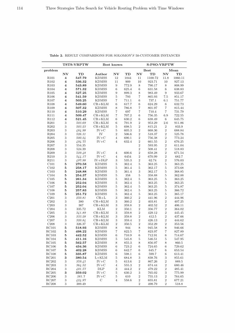
Tables 1,2 and 3 show the result comparisons, inwhich ”NV” represents the NV routes and ”TD”represents the total TD. ”Author” denotes who haveproposed the best results. The best result are presented.The best result are marked in bold indicate that, forthe instance, the TSTS-VRPTW provides new bestresult. In other cases, if the NV routes that we obtainedis equal to that of the best known, which means thatthe TSTS-VRPTW produces the best result, the bestresult is presented in italic.1) 25-Customer Instances: As shown in Table I, for25-customer instances, the TSTS-VRPTW produces29 out of 56 new best results, among which 12 comefrom the R1-type datasets, nine come from the C1-typedatasets, and eight come from the RC1-type datasets.Compared with the previous algorithms that providedthe best known, the TSTS-VRPTW has better per-formance in exploring irregular search space (datasetsR and RC). Moreover, the proposed algorithm is verygood at reducing the required NV. For the instanceswith large time windows and capacities, the requiredNV is very small. Besides the 29 new best known, theTSTS-VRPTW obtains another 14 solutions that areless than current best known solutions. Therefore, theproposed algorithm performs well in optimizing 43 outof the 56 25-customer instances.In Table 1, it can be observed that the TSTS-VRPTWcomprehensively outperforms S-PSO-VRPTW and Thecomparisons in Table I and the aforementioned investi-gation show that the proposed TSTS-VRPTW presentsa much better performance than S-PSO-VRPTW.2) 50-Customer Instances: As shown in Table 2, for50-customer instances, the TSTS-VRPTW produces 31out of 56 new best results, among which eight comefrom the RC1-type datasets, 12 come from the R1-typedatasets, nine come from the C1-type datasets, andtwo come from the RC2-type datasets. Besides, for17 of the remaining 25 instances, the TSTS-VRPTWproduces best results compared with the algorithms inthe literature. Therefore, the TSTS-VRPTW is a verypowerful technique to solve almost all the Solomon′s50-customer instances.3) 100-Customer Instances: In Table 3, results

of the TSTS-VRPTW that optimizes Solomon′s 100-customer in-stances are presented. Compared with thebest known results that are summarized on Solomon′swebsite, which is gained by 24 different algorithms,the TSTS-VRPTW obtains 38 best solutions, amongwhich two come from R2-type datasets, nine come fromC1-type datasets, eight come from RC1-type datasets,seven come from RC2-type datasets, 12 come fromR1-type datasets.

6 Conclusion

In this paper, we have proposed a set-based TS tosolve the VRPTW. In the TSTS-VRPTW, the searchspace is a universal set of arcs in the complete graph ofthe VRPTW. Each particle’s position that represents aset of delivery routes for a fleet of vehicles has been de-fined as a subset of arcs and built constructively. In thisrepresentation, the characteristics of the VRPTW havebeen fully embodied. During the construction of parti-cle position, the constraints of the VRPTW have beentaken into account, and a time-oriented NNH has beeapplied. Furthermore, a novel decision making methodhas been proposed to handle the primary and secondaryobjectives of the VRPTW. This method is not only ap-propriate for the TSTS-VRPTW, but also potentiallyuseful in other approaches to solve the VRPTW.The proposed TSTS-VRPTW is one of the few TS al-gorithm that was tested on all Solomon′s benchmarks.Experimental results illustrate the effectiveness and effi-ciency of the proposed algorithm, for we provide bet-ter results than the existing best known results forSolomon’s instances. Moreover, the TSTS-VRPTWobtains promising results on almost all the tested in-stances, which shows the robustness of the algorithm.


Table 1. RESULT COMPARISONS FOR SOLOMON′S 25-CUSTOMER INSTANCES

TSTS-VRPTW Best known S-PSO-VRPTW

problem Best MeanNV TD Authors NV TD NV TD NV TD

R101 3 302 KDMSS 8 617.1 8 618.33 8 618.33R102 3 298.92 KDMSS 7 547.1 7 548.11 7 555.14R103 3 300.22 KDMSS 5 454.6 4 473.39 4 475.21R104 3 304.33 KDMSS 4 416.9 4 418.3 4 422.47R105 3 317.1 KDMSS 6 530.5 5 556.72 5 556.3R106 3 309.69 KDMSS 3 465.4 5 466.48 5 473.22R107 3 300.71 KDMSS 4 424.3 4 425.27 4 435.44R108 3 310.318 KDMSS 4 397.3 4 405.39 4 416.14R109 3 308.26 KDMSS 5 441.3 4 460.52 4 467.25R110 3 310.56 KDMSS 4 444.1 4 445.8 4 446.45R111 3 303.85 KDMSS 5 428.8 4 429.7 4 438.66R112 3 298.20 KDMSS 4 393 4 394.1 4 400.93R201 3 299.64 CR+KLM 4 463.3 2 523.66 2 532.23R202 3 307.00 CR+KLM 4 410.5 2 455.53 2 466.97R203 3 304.92 CR+KLM 3 391.4 2 408.89 2 421.86R204 3 314.04 IV+C 2 355 1 389.91 1 398.32R205 3 320.86 CR+KLM 3 393 1 501.83 1 507.75R206 3 316.70 CR+KLM 3 374.4 1 413.21 1 431.91R207 3 301.55 KLM 3 361.6 1 402.28 1 409.43R208 3 320.23 IV+C 1 328.2 1 329.33 1 335.77R209 3 309.43 KIM 2 370.7 1 438.24 1 444.62R210 3 307.43 CR+KLM 3 404.6 1 513.98 1 526.85R211 3 310.75 KLM 2 350.9 1 361.69 1 369.86C101 3 127.28 KDMSS 3 191.3 3 191.81 3 191.81C102 3 121.57 KDMSS 3 190.3 3 190.74 3 192.29C103 3 120.28 KDMSS 3 190.3 3 190.74 3 194.12C104 3 136.69 KDMSS 3 186.9 3 187.45 3 192.45C105 3 127.28 KDMSS 3 191.3 3 191.81 3 191.81C106 3 120.34 KDMSS 3 191.3 3 191.81 3 191.81C107 3 120.28 KDMSS 3 191.3 3 191.81 3 196.09C108 3 120.28 KDMSS 3 191.3 3 191.81 3 192.22C109 3 120.08 KDMSS 3 191.3 3 191.81 3 191.84C201 3 116.7568 CR+L 2 214.7 2 215.54 2 216.98C202 3 173.95 CR+L 2 214.7 1 223.31 1 230.4C203 3 161.53 CR+L 2 214.7 1 223.31 1 229.89C204 3 177.91 CR+KLM 2 213.1 1 221.28 1 230.17C205 3 163.38 CR+L 2 214.7 1 297.45 1 297.55C206 3 184.27 CR+L 2 214.7 1 285.39 1 290.29C207 3 176.92 CR+L 2 214.5 1 274.78 1 276.26C208 3 160.78 CR+L 2 214.5 1 229.84 1 230.12RC101 3 181.64 KDMSS 4 461.1 4 462.16 4 462.39RC102 3 186.61 KDMSS 3 351.8 3 352.74 3 353.12RC103 3 180.71 KDMSS 3 332.8 3 333.92 3 334.3RC104 3 181.47 KDMSS 3 306.6 3 307.14 3 307.31RC105 3 184.25 KDMSS 4 411.3 4 412.38 4 413.73RC106 3 181.47 KDMSS 3 345.5 3 346.51 3 348.64RC107 3 191.25 KDMSS 3 298.3 3 298.95 3 303.42RC108 3 185.70 KDMSS 3 294.5 3 294.99 3 298.2RC201 3 182.62 CR+L 3 360.2 2 432.3 2 438.7RC202 3 216.27 CR+KLM 3 338 2 376.12 2 382.94RC203 3 183.39 IV+C 3 326.9 1 432.55 1 435.29RC204 3 182.11 C 3 299.7 1 327.33 1 331.4RC205 3 188.48 L+KLM 3 338 2 386.15 2 407.6RC206 3 185.1 KIM 3 324 1 482.02 1 484.79RC207 3 183.86 KLM 3 298.3 1 478.97 1 482.22RC208 3 180.70 C 2 269.1 1 309.85 1 313.17




problem Best MeanNV TD Author NV TD NV TD NV TD

R101 4 547.79 KDMSS 12 1044 11 1100.72 11.8 1060.11R102 4 536.32 KDMSS 11 909 10 923.71 10 927.13R103 4 543.89 KDMSS 9 772.9 8 790.17 8 808.99R104 4 571.32 KDMSS 6 625.4 6 631.58 6 638.83R105 4 527.25 KDMSS 9 899.3 8 983.49 9 933.67R106 4 541.59 KDMSS 5 793 7 865.93 7.5 851.17R107 4 503.25 KDMSS 7 711.1 6 737.1 6.1 751.77R108 4 549.60 CR+KLM 6 617.7 6 624.29 6 632.73R109 4 507.32 KDMSS 8 786.8 7 801.97 7 815.44R110 4 510.29 KDMSS 7 697 7 710.4 7 731.79R111 4 509.47 CR+KLM 7 707.2 6 756.35 6.9 722.55R112 4 521.45 CR+KLM 6 630.2 6 638.49 6 645.75R201 3 503.69 CR+KLM 6 791.9 2 953.29 2.6 911.86R202 3 503.23 CR+KLM 5 698.5 2 815.21 2 833.9R203 3 484.98 IV+C 5 605.3 2 668.36 2 688.84R204 3 526.31 IV 2 506.6 2 518.37 2 525.78R205 3 500.24 IV+C 4 690.1 2 756.38 2 773.24R206 3 494.75 IV+C 4 632.4 2 661.55 2 676.25R207 3 554.35 2 593.95 2 611.04R208 3 524.39 2 508.41 2 518.83R209 3 529.48 IV+C 4 600.6 2 658.28 2 671.54R210 3 544.17 IV+C 4 6454 2 670.99 2 682.7R211 3 497.98 IV+DLP 3 535.3 2 62.74 2 576.03C101 5 270.58 KDMSS 5 362.4 5 363.25 5 363.25C102 5 258.17 KDMSS 5 361.4 5 362.17 5 373.68C103 5 248.88 KDMSS 5 361.4 3 362.17 5 368.85C104 5 254.37 KDMSS 5 358 5 358.88 5 362.88C105 5 261.34 KDMSS 5 362.4 5 363.25 5 363.25C106 5 252.04 KDMSS 5 362.4 5 363.25 5 363.25C107 5 252.04 KDMSS 5 362.4 5 363.25 5 374.87C108 5 257.83 KDMSS 5 362.4 5 363.25 5 366.72C109 5 251.72 KDMSS 5 362.4 5 363.25 5 365.17C201 3 250.81 CR+L 3 360.2 2 441.96 2 444.96C202 3 380 CR+KLM 3 360.2 2 403.81 2 407.25C203 3 367 CR+KLM 3 359.8 2 402.52 2 406.11C204 3 335.72 KLM 2 350.1 2 356.77 2 364.02C205 3 341.89 CR+KLM 3 359.8 2 429.12 2 445.45C206 3 333.28 CR+KLM 3 359.8 2 412.5 2 437.66C207 3 320.84 CR+KLM 3 359.4 2 426.13 2 444.62C208 3 326.37 CR+KLM 2 350.5 2 352.29 2 353.56RC101 5 518.93 KDMSS 8 944 8 945.58 8 946.66RC102 5 498.22 KDMSS 7 822.5 7 823.97 7 827.89RC103 5 442.52 KDMSS 6 710.9 6 712.91 6 714.67RC104 5 411.16 KDMSS 5 545.8 5 546.51 5 547.95RC105 5 562.57 KDMSS 8 855.3 8 856.97 8 860.5RC106 5 434.36 KDMSS 6 723.2 6 724.65 6 729.62RC107 5 402.28 KDMSS 6 642.7 6 645.7 6 653.54RC108 5 335.87 KDMSS 6 598.1 6 599.7 6 613.41RC201 3 380.54 L+KLM 5 684.8 3 838.76 3 855.61RC202 3 359.45 IV+C 5 613.6 2 867.26 2 889.5RC203 3 364.52 IV+C 4 555.3 2 674.44 2 680.46RC204 3 401.57 DLP 3 444.2 2 479.22 2 485.41RC205 3 359.02 IV+C 5 630.2 3 765.02 3 775.99RC206 3 381.7 IV+C 5 610 2 755.13 2 764.65RC207 3 424.97 C 4 558.6 2 655.81 2 677.21RC208 3 389.49 2 498.79 2 518.8




Problem NV TD authors NV TD Best MeanNV TD NV TD

R101 8 877.05 H 19 1645.79 19 1652.00 19 1657.89R102 8 875.09 RT 17 1486.12 17 1500.81 17.8 1506.63R103 8 821.38 LLH 13 1292.68 14 1242.65 14 1268.59R104 8 860.88 M 9 1007.24 10 1042.22 10.5 1097.77R105 8 851.52 RT 14 1377.11 14 1385.08 14.3 1405.28R106 8 903.73 M 12 1251.98 12 1294.87 12.9 1287.03R107 8 845.51 S97 10 1104.66 11 1123.98 11 1160.02R108 8 776.09 BB 9 960.88 10 1011.68 10.1 1066.29R109 8 890.95 HG 11 1194.73 12 1211.63 12.4 1252.79R110 8 862.74 M 10 1118.59 11 1190.36 12 1190.38R111 8 866.58 RGP 10 1096.72 11 1102.99 11.3 1163.27R112 8 818.96 GTA 9 982.14 10 1029.12 10.8 1103.07R201 3 964.81 HG 4 1252.37 4 1274.97 4 1298.28R202 3 967.19 RGP 3 1191.70 3 1247.03 3.5 1259.84R203 3 1126.20 M 3 939.54 3 1052.71 3 1100.80R204 3 1021.90 BVH 2 825.52 3 844.16 3 928.04R205 3 1070.00 RGP 3 994.42 3 1061.46 3 1135.70R206 3 1077.00 SSSD 3 906.14 3 1016.35 3 1065.61R207 3 1052.30 BVH 2 893.33 3 946.78 3 1036.86R208 3 1036.70 M 2 726.75 2 834.72 2.6 880.31R209 3 970.64 H 3 909.16 3 1003.19 3 1076.95R210 3 1072.60 M 3 939.34 3 1040.54 3 1090.36R211 3 909.07 BVH 2 892.71 3 861.32 3 938.15C101 10 728.70 RT 10 828.94 10 828.94 10 828.94C102 10 750.30 RT 10 828.94 10 829.71 10 850.84C103 10 696.64 RT 10 828.06 10 851.37 10 886.34C104 10 651.48 RT 10 824.78 10 868.52 10 958.49C105 10 689.20 RT 10 828.94 10 828.94 10 830.44C106 10 716.50 RT 10 828.94 10 828.94 10 828.94C107 10 774.11 RT 10 828.94 10 828.94 10 865.30C108 10 721.04 RT 10 828.94 10 828.94 10 829.08C109 10 761.74 RI 10 828.94 10 828.94 10 829.58C201 3 819.66 RI 3 591.56 3 591.56 3 621.78C202 3 1017.60 RI 3 591.56 3 591.56 3 616.38C203 3 757.36 RI 3 591.17 3 591.17 3 605.84C204 3 852.70 RI 3 590.60 3 615.43 3.2 678.08C205 3 906.19 RI 3 588.88 3 588.88 3 600.31C206 3 811.08 RI 3 588.49 3 588.88 3 592.95C207 3 844.33 RI 3 588.29 3 591.35 3 596.54C208 3 913.05 RI 3 588.32 3 588.49 3 591.59RC101 9 1111.00 TBGGP 14 1696.94 15 1641.20 15 1668.88RC102 9 1097.10 TBGGP 12 1554.75 13 1510.95 13.8 1506.81RC103 9 895.30 S98 11 1261.67 11 1294.74 11.7 1305.92RC104 9 1059.80 CLM 10 1135.48 10 1190.55 10.8 1219.32RC105 9 988.04 BB 13 1629.44 14 1603.71 14.9 1581.80RC106 9 1029.00 BB 11 1424.73 12 1410.93 12.8 1416.16RC107 9 1094.50 S97 11 1230.48 11 1249.80 11.3 1277.97RC108 9 1043.50 TBGGP 10 1139.82 11 1181.87 11 1230.92RC201 3 1017.80 M 4 1406.91 4 1423.52 4 1472.71RC202 3 889.79 CC 3 1367.09 4 1193.59 4 1286.52RC203 3 998.54 CC 3 1049.62 3 1123.42 3 1222.81RC204 3 1055.00 M 3 798.41 3 894.12 3 964.50RC205 3 1018.30 M 4 1297.19 4 1321.43 4 1382.20RC206 3 913.97 H 3 1146.32 3 1307.90 4 1225.40RC207 3 926.98 BVH 3 1061.14 3 1130.37 3.7 1192.55RC208 3 1019.30 IKMUY 3 828.14 3 958.24 3 1084.93


AppendixCode for Three Function Move, Exchange and Swap

Figure 1. Algorithm 1: Move type


Figure 2. Algorithm 2: Exchange type

Figure 3. Algorithm 3: Swap type


REFERENCES

[1] N. Ando and E. Taniguchi. Travel time reliability invehicle routing and scheduling with time windows. Net-works and Spatial Economics, 6:293–311, 2006.

[2] R. Baldacci, P. Toth, and D. Vigo. Exact algorithmsfor routing problems under vehicle capacity constraints.Annals of Operation Research, 175(1):213–245, 2010.

[3] R. Bent and P.V. Hentenryck. A two-stage hybrid localsearch for the vehicle routing problem with time win-dows. Transportation Science, 38(4):515–530, 2004.

[4] J. Berger and M. Barkaoui. A parallel hybrid ge-netic algorithm for the vehicle routing problem withtime windows. Computers and Operations Research,31(12):2037–2053, 2004.

[5] O. Braysy and M. Gendreau. Vehicle routing problemwith time windows, part∥: Metaheuristics. Transporta-tion Science, 39(1):119–139, 2005.

[6] O. Braysy and M. Gendreau. Vehicle routing problemwith time windows, part|: Route construction and localsearch algorthims. Transportation Science, 39(1):104–118, 2005.

[7] A. Chabrier. Vehicle routing problem with elementaryshortest path based column generation. Computer Op-eration Research, 33(10):2972–2990, 2006.

[8] W. Cook and J.L. Rich. A parallel cutting plane al-gorithm for the vehicle routing problem with time win-dows. Working paper, Department of Computer andApplied Mathematics, Rice University, Houston, Taxas,United States of America, 1999.

[9] J. Cordeau, G. Laporte, and A. Mercier. A unified tabusearch heuristic for vehicle routing with time windows.journal of the Operation Research Society, 52:928–936,2001.

[10] Z.J. Czech and P. Czarnas. A parallel simulated an-nealing for the vehicle routing problem with time win-dows. In 10th Euromicro Workshop Parallel, DistributedNetwork-Based Process, pages 376–383, 2002.

[11] E. Danna and C.L. Pape. Column Generation, chap-ter Accelerating branch-and-price with local search: Acase study on the vehicle routing problem with timewindows, pages 99–130. Handbook of Constraint Pro-gramming. Kluwer Academic Publishers, 2005.

[12] J. Desrosiers, Y. Dumas, MM. Solomon, and F. Soumis.Network Routing, volume 8, chapter Time ConstrainedRouting and Scheduling, pages 35–139. Handbooks inOperations Research and Management Science, Amster-dam: North-Holland, 1995.

[13] L.M. Gambardella, E. Taillard, and G. Agazzi. NewIdeas in Optimization, chapter MACS-VRPTW: A Mul-tiple ant Colony System for Vehicle Routing Problemswith Time Windows, pages 63–76. McGraw-Hill, NewYork, 1999.

[14] B. Garcia, J. Potvin, and J. Rousseau. A parallel imple-mentation of the tabu search heuristic for vehicle rout-ing problems with time window constraints. Computersand Operations Research, 21(9):1025–1033, 1994.

[15] M. Gendreau, A. Hertz, and G. Laporte. New insertionand postoptimization procedures for the traveling sales-man problem. Operations Research, 40(6):1086–1094,1992.

[16] M. Gendreau, A. Hertz, and G. Laporte. A tabu searchheuristic for the vehicle routing problem. ManagementScience, 40(10):1276–1290, 1994.

[17] M. Gendreau, G. Laporte, and R. Seguin. Stochastic ve-hicle routing. European Journal of Operation Research,88:3–12, 1996.

[18] F. Glover. Future paths for integer programming andlinks to artificial intelligence. Computers and OperationResearch, 13(5):533—-549, 1986.

[19] F. Glover. Tabu search, part|. ORSA Journal on Com-puting, 1(3):190–206, 1989.

[20] F. Glover. Tabu search, part∥. ORSA Journal on Com-puting, 2(1):4–32, 1990.

[21] Y.J. Gong, J. Zhang, O. Liu, R.Z. Huang, H.S.H Chung,and Y.H. Shi. Optimizing the vehicle routing prob-lem with time windows: A discrete particle swarm op-timization approach. Ieee Transactions on Systems,Man, and Cybernetcs—part C: Applications and Re-views, 42(2):254–267, March 2012.

[22] P. Hansen. The steepest ascent mildest descent heuris-tic for combinatorial programming. Capri, Italy, 1986.Numerical Methods in Combinatorial Optimization.

[23] A. Hertz, E. Taillard, and D. Werra. A tutorial on tabusearch. Technical report, Colorado State University,http://www.cs.colostate.edu/whitley/CS640/hertz92tutorial.pdf,April 2005.

[24] J. Homberger. Verteilt-parallele Metaheuristiken zurTourenplanung. Wiesbaden: Gaber, Germany, 2000.

[25] J. Homberger and H. Gehring. Two evolutionary meta-heuristics for the vehicle routing problem with timewindows. Information System of Operation Research,37:297–318, 1999.

[26] T. Ibaraki, M. Kubo, T. Masuda, T. Uno, and M. Yag-iura. Effective local search algorithms for the vehiclerouting problem with general time windows. Work-ing paper, Department of Applied Mathematics andPhysics, Kyoto University, Japan, 2001.

[27] S. Irnich and D. Villeneuve. he shortest path problemwith k-cycle elim-ination (k ≥ 3): Improving a branch-and-price algorithm for the vrptw. Information Journalof Computer, 18(3):391–496, 2006.

[28] B. Kallehauge, J. Larsen, and O.B.G. Madsen. La-grangean duality applied on vehicle routing with timewindows - experimental results. Technical report, Infor-matics and Mathematical Modelling, Technical Univer-sity of Denmark, DTU, Richard Petersens Plads, Build-ing 321, DK-2800 Kgs. Lyngby, 2001.

[29] A. Kenyon and D. Morton. Stochastic vehicle rout-ing with random travel times. Transportation Science,37(1):69–82, 2003.

[30] G. Laporte. The vehicle routing problem: an overviewof exact and approximate algorithms. European journalof the Operation Research, 59:345–358, 1992.

[31] G. Laporte. What you should know about the vehiclerouting problem. Naval Research Logistics, 54:811–819,2007.

[32] J. Larsen. Parallelization of the vehicle routing problemwith time windows. Ph.d., Department of MathematicsModelling, Technical University of Denmark, Lyngby,Denmark, 1999.

[33] H. Li, A. Lim, and J. Hung. Local search with annealing-like restarts to solve the vrptw. Working paper, Depart-ment of Computer Science, National University, Singa-pore, 2001.


[34] X. Li, P. Tian, and S. Leung. Vehicle routing prob-lems with time windows and stochastic travel and ser-vice times: Models and algorithm. International Journalof Production Economics, 125:137–145, 2010.

[35] D. Mester. An evolutionary strategies algorithm forlarge scale vehicle routing problem with capacitate andtime windows restrictions. Working paper, The Instituteof Evolution, Haifa, Israel, 2002.

[36] Y. Rochat and E.D. Taillard. Probabilistic diversifica-tion and intensification in local search for vehicle rout-ing. Journal of Heuristics, 1(1):147–167, 1995.

[37] L.M. Rousseau, M.Gendreau, and G. Pesant. Usingconstraint-based operators to solve the vehicle rout-ing problem with time windows. journal of Heuristics,8(1):43–58, 2002.

[38] RA. Russell and TL. Urban. Vehicle routing with softtime windows and erlang travel times. Journal of theOperational Research Society, 58:1220–1228, 2008.

[39] M. Savelsbergh. private communication. 1984.

[40] G. Schrimpf, J. Schneider, H. Stamm-Wilbrandt, andG. Dueck. Record breaking optimization results usingthe ruin and recreate principle. journal of ComputerPhysic, 159(2):139–171, 2000.

[41] P. Shaw. A new local search algorithm providing highquality solutions to vehicle routing problems. Working

paper, Department of Computer Science, StrathclydeUniversity, Glasgow, Scotland, 1997.

[42] P. Shaw. Using constraint programming and local searchmethods to solve vehicle routing problems. In MaherM. and Puget J.F., editors, Principle and Practice ofConstraint Programming, pages 417–431, London,UK,1998. Springer-Verlag.

[43] MM. Solomon. Algorithms for the vehicle routing andscheduling problems with time window constraints. Op-erations Research, 35(2):254–265, 1987.

[44] W. Stewart and B. Golden. Stochastic vehicle routing:A comprehensive approach. European Journal of Oper-ational Research, 14:371–385, 1983.

[45] E. Taillard, P. Badeau, M. Gendreau, F. Guertin, andJ. Potvin. A tabu search heuristic for the vehicle rout-ing problems with soft time windows. Computers andOperations Research, 31(2):170–186, 1997.

[46] P. Toth and D. Vigo. The Vehicle Routing Problem.SIAM, Philadelphia, PA, 2001.

[47] T. VanWoensel, L. Kerbache, H. Peremans, and N. Van-daele. Routing with dynamic travel times: A queueingapproach. European Journal of Operational Research,186(3):990—-1007, 2008.

three strategies tabu search for vehicle routing problem … · capacitated vehicle routing problem...

Documents