three essays on health economics by feng pan a dissertation
TRANSCRIPT
Three Essays on Health Economics
by
Feng Pan
A dissertation submitted in partial fulfillment of the requirement for the degree of
Doctor of Philosophy (Health Services Organization and Policy and Economics)
in The University of Michigan 2009
Doctoral Committee:
Professor Dean G. Smith, Co-Chair Assistant Professor Daniel S. Silverman, Co-Chair Professor Charles C. Brown Professor A. Mark Fendrick

© Feng Pan 2009

ii
To my family, for their inspiration, love and support

iii
ACKNOWLEDGEMENTS
The writing of a dissertation can be a lonely and isolating experience, yet it is
obviously not possible without the personal and practical support of numerous people.
Thus my sincere gratitude goes to my family, my advisors, members of my dissertation
committee and all my friends for their support, encouragement, guidance and patience
over the last few years.
First and foremost, I would extend my sincere appreciation to my advisor Michael
Chernew and the members of my dissertation committee, Dean Smith, Dan Silverman,
Mark Fendrick and Charlie Brown for their time, guidance and encouragement.
Throughout my doctoral work Mike encouraged me to develop independent thinking and
research skills. Mike, along with Mark, provided me invaluable advice and help, not only
about this dissertation but also on my career development. Dean, Dan and Charlie
provided me invaluable comments on my dissertation and helped me to finish it smoothly.
I'd like to thank Allison Rosen for helping me with the tier shifting research idea
and allowing me to use Focus On Diabetes data for this dissertation. Also I wish to thank
staff from Michigan Center on the Demography of Aging data Enclave, for allowing me
to use the restricted HRS database and for helping me with the data problems.

iv
I extend many thanks to my colleagues and friends, especially Rachael Fleurence,
Sonja Sorensen, Greg De Lissovoy, Amy Huang and Luyun Chen for their
encouragement, generous support and help.
Many people on the faculty and staff of the Department of Health Management and
Policy at the University of Michigan have assisted and encouraged me in various ways
during my course of studies. I am especially grateful to Jersey Liang, Richard Hirth,
Richard Lichtenstein and Leon Wyszewianski. As an international student, I gained much
confidence from their encouragement during the early course of my graduate study.
Finally, this dissertation would not have been possible without the support from my
family. My husband Shuang Du has unwavering faith in me and supported me
unconditionally. My parents are the inspiration behind my every accomplishment. My
mother and parents in-law came from China to help me with the household work and to
take care of my young daughter. I can not thank them enough.
Chapter III “Impact of Fixed-Dose Combination Drugs On Adherence to
Prescription Medications” is a joint paper with Michael Chernew and Mark Fendrick,
part of which has been published in Journal of General Internal Medincine 23(5). Chapter
IV “The Effect of Co-payment Change on Prescription Drug Utilization-Tier shifting” is
part of Focus On Diabetes study, which is a joint work with Allison Rosen, Michael
Chernew, Mark Fendrick and Dean Smith.

v
TABLE OF CONTENTS
DEDICATION................................................................................................................... ii
ACKNOWLEDGEMENTS ............................................................................................ iii
LIST OF TABLES ........................................................................................................... vi
LIST OF FIGURES ........................................................................................................ vii
CHAPTER I INTRODUCTION .................................................................................... 1
CHAPTER II DOES “ASSET PROTECTION” ATTRACT PEOPLE TO BUY LONG-TERM CARE INSURANCE?-THE EVIDENCE FROM STATE LONG-TERM CARE INSURANCE PARTNERSHIP PROGRAM.................................. 9
CHAPTER III IMPACT OF FIXED-DOSE COMBINATION DRUGS ON
ADHERENCE TO PRESCRIPTION MEDICATIONS ....................................... 41 CHAPTER IV THE EFFECT OF CO-PAYMENT CHANGE ON
PRESCRIPTION DRUG UTILIZATION-TIER SHIFTING.............................. 74 CHAPTER V CONCLUSIONS.................................................................................. 101
vi
LIST OF TABLES
Table 2.1 Descriptive Statistics......................................................................................... 36
Table 2.2 Effects of Partnership Program: Basic Specification........................................ 37
Table 2.3 Other specification test ..................................................................................... 38
Table 3.1 Comparison of Covariates for FDC Users and Non-FDC Users ...................... 63
Table 3.2 Logit Estimates For Propensity of Using FDC................................................. 64
Table 3.3 The means during the pre-glucovance period................................................... 65
Table 3.4 Fixed Effect Estimates ...................................................................................... 66
Table 4.1 Drug Classes for Analyses................................................................................ 89
Table 4.2 Formulary Changes During Study Period......................................................... 90
Table 4.3 Study Population Treatment Use and Characteristics....................................... 91
Table 4.4 Tier Shifting Patterns ........................................................................................ 92
Table 4.5 Generic Drug Utilization Patterns – All Drug Groups ..................................... 93
Table 4.6 Generic Drug Utilization Patterns – Statins and SSRIs/SNRIs ........................ 94

vii
LIST OF FIGURES
Figure 2.1 Long-Term Care Insurance Coverage ............................................................. 33
Figure 2.2 Long-Term Care Insurance Coverage-Middle Income ................................... 34
Figure 2.3 Annual Sales of Private Long-Term Care Insurance (in thousands)............... 35
Figure 3.1 Medication Possession Ratio by Propensity Score Stratum, Before and ....... 67
Figure 3.2 Panel data Comparison on MPRs .................................................................... 68
Figure 3.3 Persistence Curves for Met/Sulf Panel ............................................................ 69
Figure 3.4 Persistence Curves for Met & Sulf Panel ........................................................ 70
Figure 4.1 Tier Distribution: Diabetic Drugs.................................................................... 95
Figure 4.2 Tier Distribution: Anti-Hypertensives............................................................. 96
Figure 4.3 Tier Distribution: Lipid Lowering Drugs ........................................................ 97
Figure 4.4 Tier Distribution: Anti-Depressants ................................................................ 98
1
CHAPTER I
INTRODUCTION
U.S. health’s share of GDP is expected to rise from 16 percent in 2004 to 20 percent
in 2015 (Borger et al 2006). Long-term care and prescription drug expenditures are
forecast to be two of the fastest growing components of health care spending (Borger et
al 2006). Changing demographics pose a great challenge on long-term care spending.
Current estimates suggest that the demand for long-term care among the elderly will
more than double in the next thirty years (Feder et al 2000). On the prescription drug side,
employers and health plans have been increasing cost sharing significantly in an attempt
to control rising drug expenditures (Dietz 2004; Robinson 2004). This dissertation
consists of three essays on health economics, with the first essay exploring long-term care
insurance market, and the other twos examining prescription drug utilizations.
Long-term care has become an important area of health economics and health care
policy, as the baby-boomers age and medical costs continue to rise. Its importance lies
not only in its share of GDP, but in how long-term care affects economic decisions for
individuals over a lifetime and across generations. Despite the high need and high cost of
long-term care, few people have purchased private long-term care insurance. In 2004,
national aggregate long-term care expenditure exceeds $130 billion, of which one third
2
was paid for out of pocket by individuals and their families, more than 60% by Medicaid
and Medicare, while only 4% was covered by private long-term care policy
(Congressional Budget Office 2004).
Extensive theoretical literature has proposed several potential reasons for the lack of
demand for private long-term care insurance. One of the most famous papers by Pauly
(1990) provided two explanations. First, insurance serves primarily to protect assets.
Because long-term care usually happens at the end of life, the value of protecting assets at
that time may not worth the trade-off from current consumption. Given the presence of
Medicaid, which may serve as a substitute for private financing when elderly exhaust
their savings, it is rational for individuals to forgo long-term care insurance coverage
even if the insurance is offered at fair premium. Second, individuals with child might not
desire insurance because its existence could decrease the amount of informal care their
children would otherwise provide. Empirically, however, we have little evidence to
support these hypotheses. Mellor (2001) found no evidence that the availability of
children or other informal caregivers were substitutes for insurance policy. Sloan and
Norton (1997) found that adverse selections and Medicaid program affected private
demand for long-term care insurance policy, but they did not find that demand is
motivated by either bequest or exchange motives.
The goal of chapter II is to use empirical evidence to explore why so few people
purchased long-term care insurance. Specifically, the effects of state long-term care
partnership programs on long-term care insurance purchase are evaluated to test the
“asset protection” hypothesis. The partnership programs are a hybrid of the public/private
approach to finance long-term care services. Currently operating in four states, the
3
programs allow individuals who buy long-term care insurance policies under the program
to protect a certain amount of their assets and become eligible for Medicaid after they
exhaust their policy benefits. Traditionally, Medicaid applicants cannot have assets that
exceed certain thresholds and must “spend down” or deplete as much of their assets as is
required to meet financial eligibility thresholds. To encourage the purchase of private
insurance, especially among moderate-income people, the partnership programs allow
long-term care insurance policyholders to protect some or all of their assets from
Medicaid spend-down requirements during the eligibility determination process, though
the four states vary in how they protect their policyholders’ assets.
Patient adherence to prescription medications has always been a problem in the
management of their illnesses, especially for those with a chronic condition. Poor medical
adherence is often associated with undesired health outcome and higher medical costs
(McCombs et al 1994). It is estimated that 10% of hospital admissions and 23% of
admissions to nursing homes in the United States are due to the complications from
medical non-adherence, costing the health care system $100 billion each year (Vermeire,
et al 2001). The goal of chapter III is to evaluate whether reducing number of drugs
improved patient adherence to medication.
The complexity of the drug regimens is often considered as an important
determinant of non-adherence (Vermeire et. al, 2001), especially in people with long
period of treatment. The complexity of drug regimen involves both the frequency of
expected intake and the number of pills needed to take. Studies have shown that
compliance rate is negatively associated with the frequency of daily drug intake (Cramer,
et. al., 1989; Detry, et al 1994; Dezii, et al 2002). There is, as yet, relatively little
4
adherence information about patients who must take more than one medication, relative
to those who are on monotherapy, for a specific illness. However, it seems intuitive that
with every additional medication a patient must take —each with its own dosing
instructions — the potential for error becomes greater.
Fixed dose combination (FDC) drugs are combinations of two or more existing
drugs produced in a single tablet to either treat one disease with complimentary actions or
treat multiple conditions. Development and marketing of FDCs are becoming
increasingly popular, partly due to the fact that for many chronic clinical conditions,
evidence-based recommendations require multiple agents to be used simultaneously in
complex regimens. FDC drugs have been approved in many therapeutic areas, especially
chronic disease treatments like diabetes, lipidemia and hypertension etc. The advocates of
FDC drugs expect that patients taking these pills could have better compliance than those
with multi-pill therapies, as the reduced number of pills diminishes the complexity of the
regiment (Wertheimer et al, 2002; Leichter, et al, 2003). Chapter III uses both fixed effect
model and propensity score method to explore the effect of Glucovance®, a FDC of
metformin and glyburide used to treat hyperglycemia in diabetes mellitus, on patient
adherence, compared to a multi-pill regimen.
In response to increasing prescription drug costs, many employers and health plans
have raised drug co-payments. Unfortunately, the evidence suggests that medication cost-
sharing indiscriminately reduces the use of both excess and essential medications alike
(Ellis et al 2004). In turn, growing evidence suggests that individuals who decrease
medication utilization due to out of pocket (OOP) costs have poorer health outcomes
5
(Piette et al 2004; Heisler et al 2004) and may even incur increases in overall health care
costs (Soumerai, et al 1991).
In response to the growing evidence that ‘one-size fits all’ co-payment harm
patients and may even increase costs, a more nuanced approach to health insurance
benefits design, in which patients’ co-payments are based on the expected clinical benefit
of the prescribed drug(s) rather than their acquisition cost, was proposed (Chernew et al
2000; Fendrick et al 2001). Under this Value Based Insurance Design (VBID) theory, the
more beneficial the medication, the lower the co-payment, thereby effectively realigning
the incentives faced by patients to increase utilization of and adherence to the most
beneficial and valuable prescription medications.
Focus On Diabetes (FOD) intervention implemented at the University of Michigan
(UM) is the first of its kind designed both to improve the quality of care for UM
employees, and to allow for a rigorous evaluation of such a program’s effectiveness. The
intervention started from July 1, 2006 and provided all UM employees and dependents
identified as having diabetes with co-payment reductions for all glycemic agents, anti-
hypertensives, lipid lowering agents, and anti-depressants.
One of the important impacts of FOD intervention is patients’ drug utilization
pattern change. A three-tier formulary is provided to UM employees and their dependents,
requiring the lowest co-payments for generic drugs (tier 1), a higher co-payment for the
brand-name drugs that are preferred by the health plan (tier 2), and the highest co-
payments for brand-name drugs that are not preferred by the health plan (tier 3). The co-
payment reductions in FOD intervention were designed to maintain the underlying
incentive structure of the formulary such that generic medications (tier 1) had larger co-
6
payment reductions than branded medications, and preferred brands (tier 2) had larger co-
payment reductions than tier 3.
How the graded co-payment changes within tiered formulary affect patient tier
utilization pattern has important implication to health plan, as the possible more
utilization on non-preferred mediations could impose unnecessary higher costs to health
plan. Previous studies have found that the adaptation of an incentive-based formulary
and/or increase co-payments resulted in switching to lower tier medications. However it
is not clear whether FOD intervention will result in more non-preferred drug utilization
or not.
The goal of chapter IV is to evaluate the effects of the FOD intervention on drug
utilizations. Specifically, how changes in co-payment reductions affected patient tier
switching within drug class is examined in chapter IV. And non-UM enrollees from the
same health plan provider (M-CARE) serve as control group in the study, as their
employers did not provide such co-payment reductions on these drugs.
7
References Borger C. et al “Health Spending Projections Through 2015: Changes On The Horizon”
Health Affairs 2006 25(2) w61 Chernew, ME; Encinosa WE; Hirth RA “Optimal health insurance: the case of
observable, severe illness” Journal of Health Economics 2000 19(5): p. 585-609 Cramer, JA et al “How often is medication taken as prescribed?” JAMA, 1989 Congressional Budget Office (CBO). “Financing Long-Term Care for the Elderly.”
Government Printing Office: Washington, DC. 2004 April. Dezii, CM et al “Effects of once-daily and twice-daily dosing on adherence with
prescribed Glipizide oral therapy for type 2 diabetes” Southern Medical Journal, 2002
Detry, et al “Patient compliance and therapeutic coverage: amlodipine vs nifedipine in
the treatment of angina pectoris.” Journal of General Internal Medicine, 1994 Dietz, E., “Trend in employer-provided prescription drug coverage”. Monthly Labor
Review, 2004. 127(8): p. 37-45. Ellis, J.J., et al., “Suboptimal statin adherence and discontinuation in primary and
secondary prevention populations. Should we target patients with the most to gain?” J Gen Intern Med, 2004. 19(6): p. 638-645.
Feder J. et al “Long-Term Care In The United States: An Overview” Health Affairs 2000
19 (3) Fendrick, A.M., et al., “A benefit-based copay for prescription drugs: patient contribution
based on total benefits, not on drug acquisition cost”. Am J Manag Care, 2001. 7: p. 861-867.
Heisler, M., et al., “The health effects of restricting prescription medication use because
of cost.” Med Care, 2004. 42(7): p. 626-634. Leichter, S.B. and Thomas, S. “Combination Medications in Diabetes Care: An
Opportunity that Merits More Attention” Clinical Diabetes, 22(4) 2003 McCombs, J.S., Nichol, M.B., Newman, C.M., Sclar, D.A. The costs of interrupting
antihypertensive drug therapy in a medicaid population. Medical Care. 1994; 32(3): 214-216.
Mellor JM. Long-term care and nursing home coverage: are adult children substitutes for
insurance policies? Journal of Health Economics 2001 20 527-547

8
Pauly, M.V. “The Rational Nonpurchase of Long-Term-Care Insurance” The Journal of
Political Economy, Vol. 98, No. 1 (Feb., 1990), pp. 153-168 Piette, J.D., et al., “Health insurance status, cost-related medication underuse, and
outcomes among diabetes patients in three systems of care.” Med care, 2004. 42: p. 102-109.
Robinson, J.C., “Reinvention of health insurance in the consumer era”. JAMA, 2004.
291(15): p. 1880-1886.
Sloan FA and Norton EC, Adverse Selection, Bequests, Crowding Out, and Private Demand for Insurance: Evidence from the Long-term Care Insurance Market. Journal of Risk and Uncertainty, 1997 15: 201-219
Soumerai, S.B., et al., “Effects of Medicaid drug-payment limits on admission to
hospitals and nursing homes.” New England Journal of Medicine, 1991. 325(15): p. 1072-1077.
Vermeire, E., Hearnshaw, H., Van Royen, P and Denekens, J. Patient adherence to
treatment: three decades of research. A comprehensive review. Journal of Clinical Pharmacy and Therapeutics. 2001; 26(5): 331-342.
Wertheimer, A.I., Morrison, A. Combination Drugs: Innovation in Pharmacotherapy.
P&T; 2002, 27(1): 44-49.

9
CHAPTER II
DOES “ASSET PROTECTION” ATTRACT PEOPLE TO BUY
LONG-TERM CARE INSURANCE?-THE EVIDENCE FROM
STATE LONG-TERM CARE INSURANCE PARTNERSHIP
PROGRAM
As Americans are enjoying longer life than ever, the need for appropriate long-term
care is also growing. It is estimated that people aged 80 years old and above –those most
likely to need long-term care – will be increased by about 60% between 2002 and 2020
(Lakdawalla and Philipson, 2001). And today’s 65 year old faces a 24% chance of having
a year or longer nursing home stay sometime during his or her remaining life (Spillman
and Becker, 2005a). Long-term care is very expensive. Nursing home costs in 2004 range
from $30,000 to $65,000 per year, and care provided at home can cost up to $19 per hour
(Metlife Mature Market Institute, 2006).
However, despite the high need and high cost of long-term care, few people have
purchased private long-term care insurance. In 2004, national aggregate long-term care
expenditure exceeds $130 billion, of which one third was paid for out of pocket by
individuals and their families, more than 60% by Medicaid and Medicare, while only 4%
was covered by private long-term care policy (Congressional Budget Office 2004). By
contrast, in the health sector as a whole, private insurance pays for 35% of expenditure

10
and only 17% are paid for out of pocket (National Center for Health Statistics, 2002). The
limited insurance coverage for long-term care has important impact for the welfare of the
elderly and potentially for their adult children too, as children may have to provide
informal care to substitute the formal care. The importance will become more
pronounced when the baby-boomers age and medical costs continue to rise.
Extensive theoretical literature has proposed several potential reasons for the lack of
demand for private long-term care insurance. On the supply side, market function may be
impaired by adverse selection, moral hazard, high transaction costs, imperfect
competition or dynamic problems with long-term contracting (Norton, 2000). On the
demand side, difficulty understanding low-probability high loss events or misconceptions
about the extent of public health insurance coverage for long-term care (Kunreuther 1978)
may play a role. One of the most famous papers by Pauly (1990) provided two additional
explanations. First, insurance serves primarily to protect assets. Because long-term care
usually happens at the end of life, the value of protecting assets at that time may not
worth the trade-off from current consumption. Given the presence of Medicaid, which
may serve as a substitute for private financing when elderly exhaust their savings, it is
rational for individuals to forgo long-term care insurance coverage even if the insurance
is offered at fair premium. Second, individuals with children might not desire insurance
because its existence could decrease the amount of informal care their children would
otherwise provide.
Yet despite these extensive theoretical literatures, we have little empirical evidence to
support these hypotheses or provide additional explanations. Brown and Finkelstein
(2007) have found that higher premium mark up did limit the purchase of long-term care

11
insurance. However, they also suggest that supply-side market failure is not sufficient to
explain the very small size of long-term care insurance market. Mellor (2001) found no
evidence that the availability of children or other informal caregivers were substitutes for
insurance policy. Sloan and Morton (1997) found that adverse selections and Medicaid
program affected private demand for long-term care insurance policy, but they did not
find that demand is motivated by either bequest or exchange motives.
In this chapter, I used additional evidence to test the “asset protection” hypothesis.
Medicaid, the joint federal-state health financing program for low-income individuals,
pays for long-term care, but only for those who have exhausted nearly all of their own
resources first. To receive coverage, individuals must “spend down” their assets and
demonstrate that virtually all of their income is being used to pay for their care. Given the
fact that Medicaid is not a perfect substitution for private insurance, crowd-out effect
from Medicaid may be due to the fact that people has little incentive to protect their asset
at the end of life when long term care usually happen (Pauly, 1990). Empirically,
however, purchasing a long-term care policy, for most seniors or near seniors, does not
guarantee a certain level of asset protection because there remains the risk that they will
need long-term care beyond the terms of the private insurance, although they could get
better care under private insurance. That is even people purchase LTC insurance, they
may exhaust their coverage under the policies and have to deplete their savings to seek
Medicaid coverage eventually.
The state long-term care partnership programs offer a natural experiment to test the
“asset protection” hypothesis. The partnership programs are a hybrid of the public/private
approach to finance long-term care services. Currently operating in four states —

12
California, Connecticut, Indiana, and New York, implemented since 1994, 1992, 1993
and 1993 respectively — the programs allow individuals who buy long-term care
insurance policies under the program to protect a certain amount of their assets and
become eligible for Medicaid after they exhaust their policy benefits. Traditionally,
Medicaid applicants cannot have assets that exceed certain thresholds and must “spend
down” or deplete as much of their assets as is required to meet financial eligibility
thresholds. To encourage the purchase of private insurance, especially among moderate-
income people, the partnership programs allow long-term care insurance policyholders to
protect some or all of their assets from Medicaid spend-down requirements during the
eligibility determination process, though the four states vary in how they protect their
policyholders’ assets.
Using data from Health Retirement Study (1992-2004) and difference-in-difference
method, I did a longitudinal analysis of the private long-term care insurance purchasing. I
did not find that implementation of long-term care partnership program significantly
increase the LTC insurance coverage among the general population and among some
subgroups as well. The results, to some extent, support existing theories that protecting
asset and leaving bequests to children and spouse are not attracting people to purchase
private long-term care insurance coverage.
The chapter proceeds as follows: In section 1, I show the background information on
long-term care market, state long-term care insurance partnership programs, and existing
theories and empirical evidences on limited private insurance market. In section 2, I
describe the empirical methods used, including econometric models, data source and

13
covariates. In section 3, I present the empirical estimates, followed with discussion of
implications and limitation in section 4.
1. BACKGROUND
1.1 Public and Private Coverage for Long Term Care
Long-term care has become an important area of health economics and health care
policy, as the baby-boomers age and medical costs continue to rise. Its importance lies
not only in its share of GDP but in how long-term care affects economic decisions for
individuals over a lifetime and across generations. Long-term care is used by people who
need assistance to function in their daily lives. Caring for a chronic illness lasts as long as
a person is alive so that medical expenses accumulate unrelentingly. Long-term care is
often provided by unpaid caregivers. Many elderly people receive informal care from
friends or family, often a spouse or child, in the home. In 1999, two-thirds of older people
with disabilities residing in the community relied exclusively on informal, or unpaid, help.
Of those who used any formal or paid help, about three-fourths also received unpaid care
from friends and family (Spillman and Black, 2005b).
The formal care can be very costly. In 2006, the average cost of care in a nursing
home was about $75,000 for a private room and $67,000 for a shared room. In the same
year, the average private payment for a home health aide to provide care at home was $19
per hour (Metlife Mature Market Institute, 2006). Assisted living rates averaged $35,600
per year in 2006. Rates vary, depending on region, size of the accommodations, services
available, quality of care, and amenities (Metlife Mature Market Institute, 2006).
The Medicaid program is the nation’s major source of public financing for long-term
care. The Medicaid program accounts for 44 percent of the $173 billion spent in 2001 for

14
long-term care. Another public health insurance program-Medicare, pays about 17% of
the total long-term care expenditure.
Neither Medicaid nor Medicare is an adequate solution for long term care coverage.
Medicaid is a means-tested program whereby individuals are covered only if they do not
have enough income, assets and insurance to pay for the care. To receive coverage,
individuals must “spend down” their countable assets (exempt assets include a home, a
car, and funds designated for burial expenses) and demonstrate that virtually all of their
income is being used to pay for their care (eligibility rules varies across states). Although
special rules allow married couples to set aside income and assets for a community
spouse, many states allow community spouses to keep only the federal minimum levels
of income and assets. Critics on the “spend down” rules suggest that higher-income
elderly may transfer their assets to their children to preserve their bequests and have
Medicaid pay for their long-term care services. However, empirical researches
demonstrate that very few people transferred their asset to be eligible for Medicaid
(O’Brien E, 2005).
Medicare is a federal program that is available to most people at age 65. But it only
has the potential to pay for up to a maximum of 100 days in a skilled nursing facility and
requires that beneficiary has a 72 hour hospital stay prior to entering the nursing home. In
general, Medicare does not adequately cover long-term care expenses. It requires that
patients are getting better or showing improvement.
Private coverage of long-term care is very limited. Relatively few older persons have
private insurance that covers the cost of long-term care. By 2005, roughly 7 million LTC
policies were in force in the United States, and about 10% of Americans over the age of
15
55 have private insurance protection (America’s Health Insurance Plan 2007). Although
the private coverage has increased significantly since 1990, only 4% of long-term care
expenditure was covered by private insurance (Congressional Budget Office 2004).
People without public and private coverage of long-term care have to pay for the care out
of pocket, which accounts for almost one third of the long-term care expenditure
(Congressional Budget Office 2004).
1.2 Theories and Empirical Evidences
Given the high cost and high probability of long-term care, private insurance should
have been attractive to a risk-averse person if there is no supply side market failure. First
Purchase of LTC insurance would provide people with coverage when they need LTC
services. Without private coverage, they have to pay the services out-of-pocket until they
exhaust their savings and be eligible for Medicaid. Under such circumstance they don’t
have money left for their own and a surviving spouse' comforts or to leave a bequest for
children. Second, LTC insurance provides flexibility in choosing care options in the event
LTC becomes necessary.
The fact that only a few percent of elderly have purchased private long-term care
insurance has been the subject of much theoretical research. The tendency to ignore low-
probability, high-loss events that have not occurred recently has been proposed in earlier
work (Kunreuther, 1978) as one possible explanation for the limited private long-term
care. However this sort of behavior has not been so common in health insurance. Another
most common explanation is that the elderly are misinformed. A majority of the elderly,
according to survey, is under the mistaken impression that Medicare already provides
long-term care coverage (American Association of Retired Persons, 1985). On the supply
16
side, pricing problems, moral hazard and adverse selection were proposed to explain the
limited market (Davis and Rowland 1986).
Based on utility maximization models, Pauly (1990) proposed alternative reasons to
explain the low coverage of long-term care. He argued that given these reasons, risk-
averse, rational and appropriately informed individuals would not buy LTC insurance
even if the insurance were offered at fair premiums and there is no loading and adverse
selection.
Pauly argued that insurance serves primarily to protect assets. In the case of long-term
care, because chronic illness is not curable, utility in the “sick state” is far less than that
in the “healthy state”. The marginal utility from the consumptions at the sick state in the
future may not worth the trade-off from current consumption at healthy state. That is the
gain to a risk-averse person from buying coverage against LTC costs is less than the gain
from insuring an acute care expense of equal amount. Given the presence of Medicaid,
which may serve as a substitute for private financing when elderly exhaust their savings,
it is rational for individuals to forgo long-term care insurance coverage even if the
insurance is offered at fair premium with modest load.
On the other hand, if long-term care insurance is serve to protect bequest, the greater
the utility from bequests and the less sharply marginal utility from bequest declines with
age, the greater the demand for LTC insurance. However, Pauly also proposed an
intrafamily bargaining hypothesis that individuals with children might not desire
insurance because its existence could decrease the amount of informal care their children
would otherwise provide. That is the elderly may fear that if they purchase insurance
children may institutionalize them when they will be unable to act on their own.
17
However, despite these extensive theoretical literatures, we have little empirical
evidence to support these hypotheses or provide additional explanations. Brown and
Finkelstein (2007) have found that higher premium mark up did limit the purchase of
long-term care insurance. However, they also suggest that supply-side market failure is
not sufficient to explain the very small size of long-term care insurance market, as they
found enormous gender differences in pricing that do not translate to differences in
coverage. Using different data and analysis method, Cramer et al (2006) also suggests
that demand for LTC insurance is very price inelastic, although price was a significant
determinant in decisions to purchase LTC coverage1.
A couple of empirical papers have tested Pauly’s child substitution hypothesis. Mellor
(2001) found no evidence that the availability of children or other informal caregivers
were substitutes for insurance policy. Sloan and Morton (1997) did not find that demand
for long-term care insurance is motivated by either bequest or child substitution.
The Medicaid crowd-out hypothesis has been supported by several studies. Sloan and
Morton (1997) found evidence that Medicaid crowds out demand for private LTC
insurance for persons over age 70 but not for persons in the 51-64 cohort. Brown and
Finkelstein (2004) quantified the impact of Medicaid, i.e. the amount by which private
LTC coverage would duplicate coverage that would be provided by Medicaid, once the
person’s assets were depleted. The duplication increased as the wealth decreased.
Medicaid would be duplicative of more than half the private LTC coverage in the lower
half of the wealth distribution.
1 The authors used a logit model to predict the purchase of new LTC policy and found that price was a statistically significant predictor. However, when they calculated the marginal effect on probability of buying long-term care insurance, they found that the price elasticity was very small
18
Sparse empirical evidence to explain small private LTC insurance market has limited
implication on public policy. Inelastic demand and Medicaid crowd out evidence
suggested that government initiations focusing on LTC insurance price reduction would
meet with little success. If Pauly’s hypothesis (1990) that lack of incentive to protect
assets and bequests is the reason of non-purchase of LTC insurance holds true, any
incentives created by policies would be counteracted
In this chapter, I used empirical evidence to test the “asset/bequest protection”
hypothesis. State long-term care partnership programs provided a natural experiment for
such analysis.
1.3 State Long-Term Care Partnership Program
Over the years, several initiatives aimed at increasing LTC insurance sales have
focused on ways to make private LTC insurance policies more attractive. The partnership
for long-term care is one of the major interventions (General Accounting Office, 2005).
The long-term care partnership program began in 1987 as a demonstration project
funded through the Robert Wood Johnson Foundation. The program is a public-private
partnership designed to encourage persons with moderate income to purchase private
long-term care insurance to fund their long-term care needs rather than relying on
Medicaid. Individuals who buy a partnership policy and eventually need long-term care
services first rely on benefits from their private long-term care insurance policy to cover
long-term care costs. If the policyholders exhaust private long-term care insurance
benefits and need assistance from Medicaid to fund LTC, they may protect some or all of
their assets from Medicaid spend-down requirements during the eligibility determination
process, though they are still subject to Medicaid income requirement. One goal of the
19
program is to save money for Medicaid by delaying or eliminating the need for
participants to access Medicaid for long-term care services.
As part of the demonstration project, four states—California, Connecticut, Indiana,
and New York—developed partnership programs since 1994, 1992, 1993 and 1993
respectively. No more states implemented the program until 2006 after congress
approved legislation clearing the way for expanded nationwide LTC partnerships.
The four states with partnership programs offer one of three program models to protect
buyers’ assets: dollar-for-dollar, total asset protection and hybrid. Under dollar-for-dollar
model, assets are protected up to the amount of the private insurance benefit paid, while
total asset protection model protects all assets when a state-defined minimum benefit
package is paid. The hybrid model offers both dollar-for-dollar and total asset protection.
The type of asset protection depends on the initial amount of coverage purchased. Total
asset protection is available for policies with initial coverage amounts greater than or
equal to a coverage level defined by the state.
2. EMPIRICAL METHODS
2.1 Hypotheses
The initial purpose of the state LTC insurance partnership program is to reduce Medicaid
spending by encouraging people to purchase private insurance. No expectation on the
uptake of LTC insurance policies under the program is found in the literature. As the
available information was insufficient in terms of selecting a null hypothesis on the effect
of the program, my hypotheses are that the uptake of LTC insurance policies in the
experimental states is not different from zero, when compared to non-partnership states,
among both general population and subgroups including higher income population, those
20
with children and married couples.. Also, based on Pauly’s theories, “asset protection”
from LTC partnership program may not attract people to buy private coverage. People
who buy policies under the partnership program would have bought private coverage if
there were not partnership programs. That is the partnership program would just have a
crowd-out effect: it would crowd out the purchase of regular LTC insurance policies.
2.2 Data
Health and Retirement Study (HRS) data is used for this study. HRS is an on-going,
nationally representative survey of older adults in the United States. HRS survey started
from 1992. More than 10,000 Americans between the age of 50s and 60s (in 1992) were
interviewed every two years. HRS survey contains a wide variety of information on
health conditions, insurance coverage, family composition and financial resources. The
survey specially asked the respondents about their private long-term care insurance
coverage, which states, “Do you have any type of supplementary health insurance
coverage, such as Medigap or long-term care insurance that is purchased directly from an
insurance company or through a membership organization such as AARP. If yes, what
coverage do you have? ”(1992 and 1994 questionnaire, although people were asked for
general supplementary coverage first, long-term care insurance is listed separately for
interviewees to check); “Not including government programs, do you have any insurance
which specifically pays any part of long-term care, such as personal or medical care in
your home or in a nursing home?” (post-1996 questionnaire).
HRS data has been used by several empirical studies for the purpose of LTC
insurance analysis (Mellor 2001, Cramer and Jensen 2006, Sloan and Norton 1997), some
of which are widely cited (Mellor 2001, Sloan and Norton 1997).
21
For the purpose of this study, pooled HRS data from 1992 to 2004 (7 waves) is used
to evaluate the effect of the programs on long-term care insurance purchasing. Since
Connecticut started the partnership program in 1992 and I use difference-in-difference
method to evaluate the program impact, residents from Connecticut are excluded from
the study sample. In addition, only respondents are included in the analysis. Responders’
spouses who are not respondents are excluded.
Although the rest three partnership program states (California, New York and Indiana)
initiated the programs in 1994, 1993 and 1993 respectively, the true implementation year
could be considered as the next year following initiation. Because HRS survey asked
about events that most likely happened in the previous year, the pre-intervention HRS
waves are actually 1992 and 1994, and 1996-2004 (the rest 5 waves) are post-intervention
period.
One limitation of the HRS data is that it is restricted to a fixed cohort-those who were
50-60 year old in 1992.
2.3 Econometric Models
Difference-in-difference (DD) estimation has been a commonly used method to
estimate causal relationships. The great appeal of DD estimation comes from its
simplicity as well as its potential to circumvent many of the endogeneity problems that
typically arise when making comparisons between heterogeneous individuals (Bertrand,
et al 2004).
Following previous studies such as Gruber and Poterba (1994), I assume that an
individual’s underlying demand for long-term care insurance, *iI , can be described as a
22
vector of socio-demographic characteristics Xi, income and assets Yi, and state-
partnership program policy Pj:
itjjjitititj PostPPostPYXI εδδδαβ +++++= 321* *** (1)
Where i indexes individuals, j states, and t years. P is set equal to 1 if the individual is
a residence of one of the partnership states an zero otherwise. Post is set to one for years
after partnership is implemented in the data (years after 1994), and is zero previously.
P*Post thus captures the change in demand for long-term care insurance for residences of
partnership states, relative to the residences of non-partnership states, after the
implementation of the program.
In practice, *iI is unobservable. We observe instead a dummy variable, defined by
Ii=1 if *iI >0, and Ii =0 otherwise. The error term in the demand equation is assumed to
follow a normal distribution. And the parameters are estimated by fitting the pooled HRS
data to a probit model.
In additional to the above base model, four more models were estimated to evaluate
the effects of asset protection on different populations. The first model has exactly the
same specification as the base model, except that it is restricted to individuals with
relatively higher income. The rationale for the test is that the partnership is targeted at
middle or higher income group, who face the risk of depleting their life-time savings to
be eligible for Medicaid if long-term care needed. The higher income group is defined as
those whose income per person was greater than $25,000 per year at 1992 dollars. The
second model explored if the partnership states have different LTC insurance demand
trend than the non-partnership states during the post intervention period. The third and
fourth models tested whether individuals with child or spouse are more likely to be
23
attracted by “asset protection”, given the assumption that the protected asset is most
likely to be bequest.
The subgroup analyses are done in two ways. A separate equation is run for higher
income group while interaction terms are used for those with children or spouse. There
are two reasons. First, as the parameters for interaction terms are measuring relative
effect instead of absolute effect, the separate equation is run for high income group to
directly get the absolute effect of partnership program on this sub group. Second,
population characteristics may differ by income (e.g. race, education, health status etc),
but not significantly by marital status and whether having children. Therefore we may
expect that some of the parameters of the higher income group are different from those of
the general population.
2.4 Covariates
The selection of model covariates is based on previous empirical evidence and
theoretical hypothesis. Besides the key independent variables like partnership state and
post intervention indicator, the factors that might affect the demand for LTC insurance
include demographics, wealth, health status, health services utilizations during the year
and state dummies.
The demographic variables include age, gender, education marital status, whether
having child, and race and ethnicity. Women are expected to be more likely to purchase
LTC insurance because they have a longer life expectancy, implying a higher probability
of needing care and of needing it for a longer period of time. Married persons would
purchase LTC insurance, because ‘impoverishing one’s spouse… seems to be the major
fear of many married elderly” (Pauly, 1990). More educated people are expected to be
24
less ‘myopic” and more informed, and thus might have higher chance of buying LTC
insurance. Because informal child-provided care is a possible substitute for formal LTC,
those with children would have lower probability of buying LTC insurance. Race and
ethnicity variables are intended to capture cultural differences that might affect the
decision to purchase LTC insurance. White is expected to have higher probability to
purchase LTC insurance than the minority groups as minority groups tend to use more
informal care.
Wealth variables include personal annual income and non-house asset, which are
adjusted to 1992 dollars (the base year). The wealthier individuals are expected to be
more likely to purchase LTC insurance, since they have lower probability to get Medicaid
coverage.
Health status includes self-reported health status, number of ADLs (disability
measurement), and number of comorbidities. Health services utilization includes whether
hospitalized during the year and whether having nursing home stay during the year. The
hypothesis is that people who are “sicker” might expect they may use LTC in the future
and are more likely to buy LTC insurance. But on the other hand, the price of LTC
insurance for healthier individuals is cheaper than “sicker” ones, which may affect the
direction of these variables oppositely.
In addition, the demand for long-term care insurance may be affected by state
Medicaid policy. For example, higher eligibility requirements could increase people’s
demand for private insurance since it’s hard for them to get public coverage. Thus a set of
state dummy variables are included to control for policy variations across states. After
adding the state dummy variables, the coefficient of Pj in equation (1) would not be

25
identified. However, it does not affect the coefficient of the key independent variable
P*Post, which measures the effect of LTC partnership program. Also, although some of
the state Medicaid policies changed during the study period, none of the partnership
states implemented Medicaid policy changes during the same year they started the
partnership program. For non-partnership states, some minor Medicaid policy changes
were implemented around the intervention years, including changing Medicaid
reimbursement rates, minor changes on eligibility rules etc. However, these Medicaid
policy changes are expected to have little effect on private LTC demand, as evidences
show that they did not affect nursing home utilization (Grabowski and Gruber, 2005).
Therefore, only state fixed effect is included in the model.
Finally, since the models include 7 waves of HRS data (1992-2004), time trend (year)
is also included as a covariate.
3. RESULTS
3.1 Descriptive Results
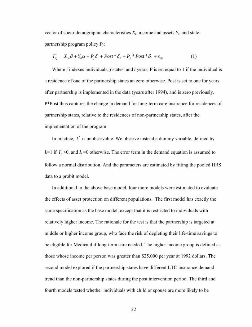
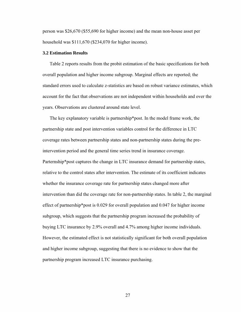
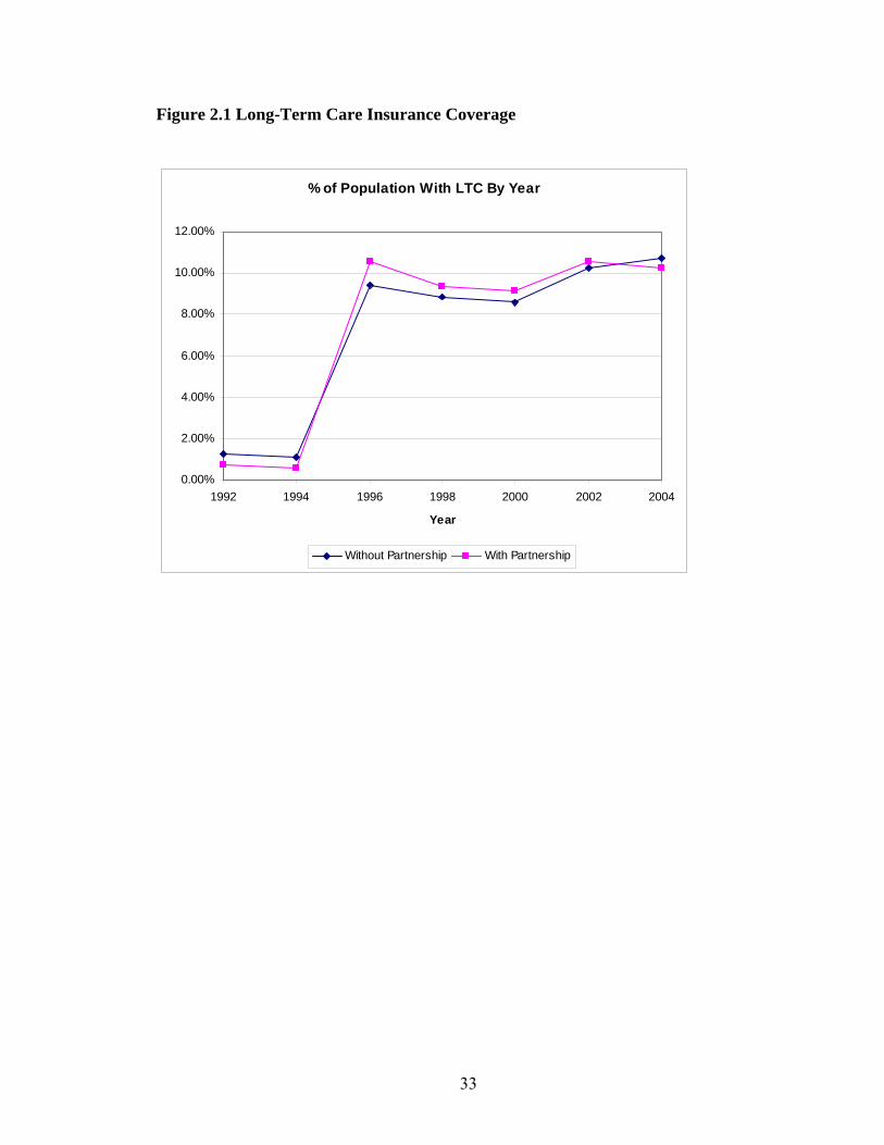
Figure 1 compares long-term care insurance coverage rates of states with partnership
program and those without over the study period (1992-2004). The rates are adjusted
using the HRS weights. During the pre-intervention period (1992-1994), mean coverage
rates for the partnership states are 0.72% (1992) and 0.6% (1994), and the rates for non-
partnership states are a little higher (1.25% for 1992, and 1.1% for 1994). During the post
period (1996-2004), however, the LTC coverage rates of the intervention states became
higher except 2004. It is noteworthy that the coverage rates for both groups jumped
significantly between 1994 and 1996. Two potential reasons might explain this. First,
according to the estimations from Health Insurance Association of America (Cohen,
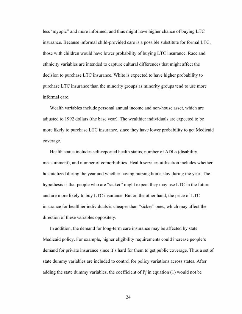
26
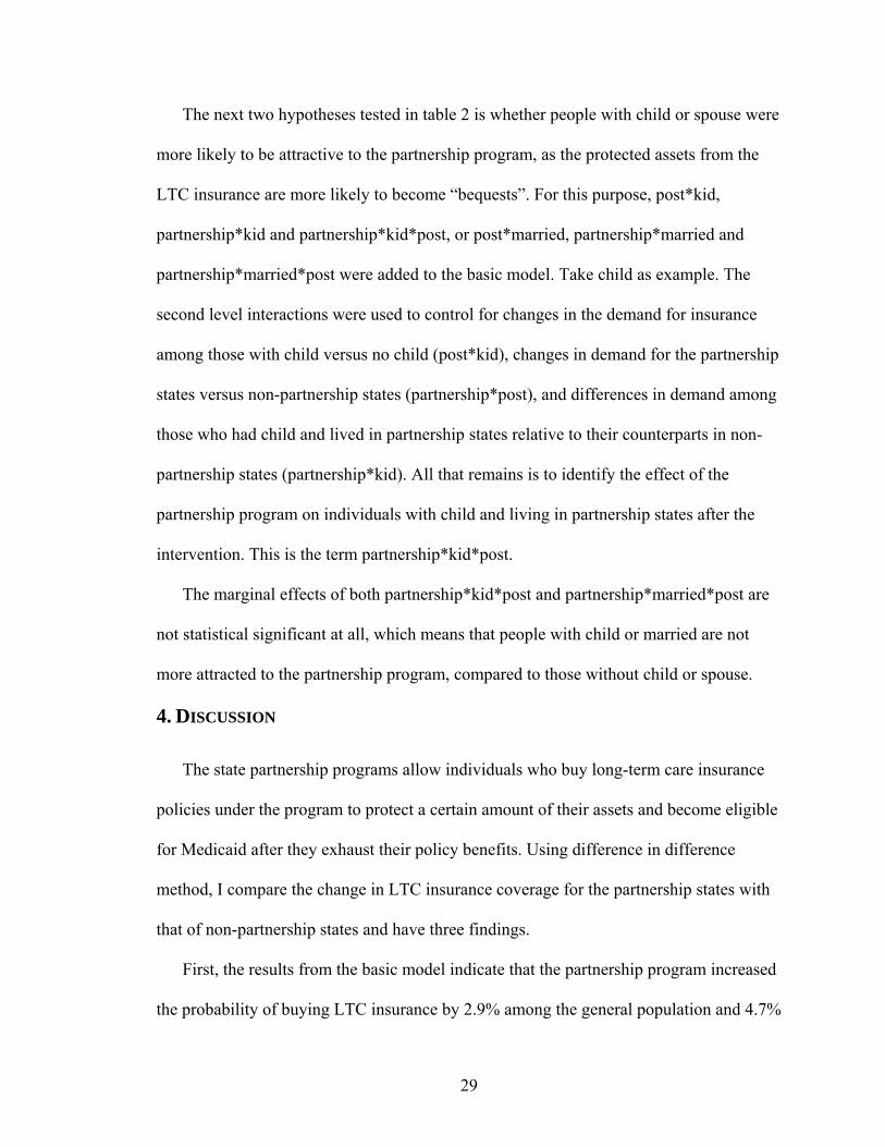
2003), the annual sales of new LTC policies grew dramatically between 1994 and 1996,
with 420,000 in 1994, 514,000 in 1995 and 609,000 in 1996 (see figure 3). The time
trend of LTC coverage in figure 1 roughly matches the annual sales of new policies trend
from Cohen (2003). These dramatic changes are mainly contributed to the efforts to
reduce supply side barriers from long-term care insurance companies. Second, HRS
changed the questionnaire on long-term care insurance coverage between 1994 and 1996,
which may cause a different interpretation from interviewees and resulted in different
answers to the question. However, this change affects control group just as if affects
treatment group. Third, the age range of 1992 HRS data is 50-60 years old (although the
spouses may fall outside this range, majority respondents from the 1992 cohort are in that
range), while the mean age of LTC insurance buyers in the individual market is 67. As
the 1992 cohort ages, their probability of buying LTC insurance also increased.
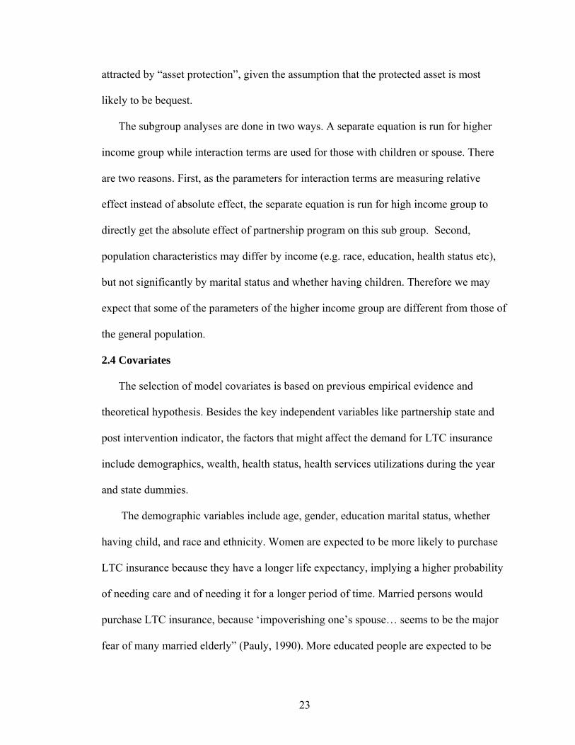
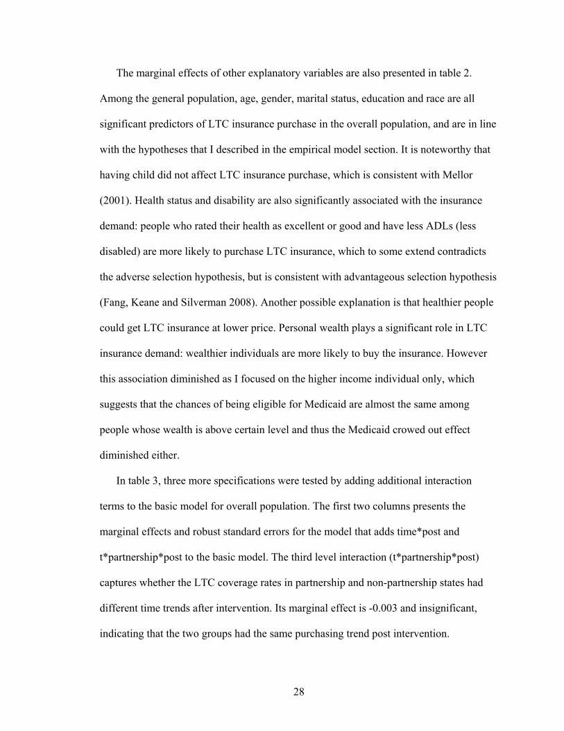
Figure 2 presents the same comparison as figure 1 but for a different group –
individuals with income higher than $25,000 in 1992 dollars. This group of people
showed similar LTC coverage trends as the overall population, but higher rates. In 1992
and 1994, the LTC coverage rates for higher income individuals were only slightly higher
than the rates of general population. However, in 1996, the coverage rates for higher
income jumped to 14%-16%, and continue to grow during the rest of years, compared to
9.5%-10.5% for overall population.
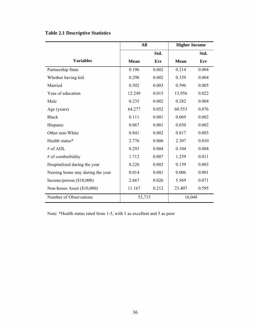
The summary statistics of the model covariates are presented in table 1. A total of
53,715 person-years (16,048 for higher income subgroup) are included in the final
analysis. 19.6% (21.4% for higher income subgroup) were living in the partnership states.
Only 23.5% (28.2% for higher income) of the sample were male. The mean income per
27
person was $26,670 ($55,690 for higher income) and the mean non-house asset per
household was $111,670 ($234,070 for higher income).
3.2 Estimation Results
Table 2 reports results from the probit estimation of the basic specifications for both
overall population and higher income subgroup. Marginal effects are reported; the
standard errors used to calculate z-statistics are based on robust variance estimates, which
account for the fact that observations are not independent within households and over the
years. Observations are clustered around state level.
The key explanatory variable is partnership*post. In the model frame work, the
partnership state and post intervention variables control for the difference in LTC
coverage rates between partnership states and non-partnership states during the pre-
intervention period and the general time series trend in insurance coverage.
Parternship*post captures the change in LTC insurance demand for partnership states,
relative to the control states after intervention. The estimate of its coefficient indicates
whether the insurance coverage rate for partnership states changed more after
intervention than did the coverage rate for non-partnership states. In table 2, the marginal
effect of partnership*post is 0.029 for overall population and 0.047 for higher income
subgroup, which suggests that the partnership program increased the probability of
buying LTC insurance by 2.9% overall and 4.7% among higher income individuals.
However, the estimated effect is not statistically significant for both overall population
and higher income subgroup, suggesting that there is no evidence to show that the
partnership program increased LTC insurance purchasing.
28
The marginal effects of other explanatory variables are also presented in table 2.
Among the general population, age, gender, marital status, education and race are all
significant predictors of LTC insurance purchase in the overall population, and are in line
with the hypotheses that I described in the empirical model section. It is noteworthy that
having child did not affect LTC insurance purchase, which is consistent with Mellor
(2001). Health status and disability are also significantly associated with the insurance
demand: people who rated their health as excellent or good and have less ADLs (less
disabled) are more likely to purchase LTC insurance, which to some extend contradicts
the adverse selection hypothesis, but is consistent with advantageous selection hypothesis
(Fang, Keane and Silverman 2008). Another possible explanation is that healthier people
could get LTC insurance at lower price. Personal wealth plays a significant role in LTC
insurance demand: wealthier individuals are more likely to buy the insurance. However
this association diminished as I focused on the higher income individual only, which
suggests that the chances of being eligible for Medicaid are almost the same among
people whose wealth is above certain level and thus the Medicaid crowed out effect
diminished either.
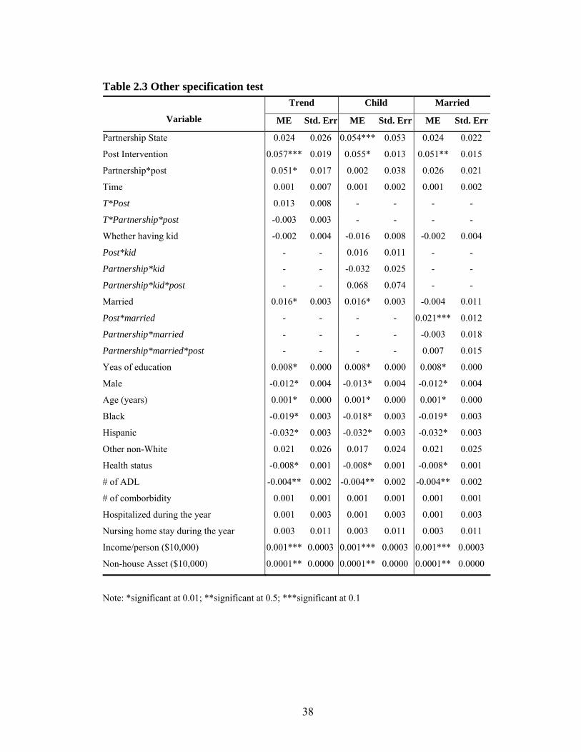
In table 3, three more specifications were tested by adding additional interaction
terms to the basic model for overall population. The first two columns presents the
marginal effects and robust standard errors for the model that adds time*post and
t*partnership*post to the basic model. The third level interaction (t*partnership*post)
captures whether the LTC coverage rates in partnership and non-partnership states had
different time trends after intervention. Its marginal effect is -0.003 and insignificant,
indicating that the two groups had the same purchasing trend post intervention.
29
The next two hypotheses tested in table 2 is whether people with child or spouse were
more likely to be attractive to the partnership program, as the protected assets from the
LTC insurance are more likely to become “bequests”. For this purpose, post*kid,
partnership*kid and partnership*kid*post, or post*married, partnership*married and
partnership*married*post were added to the basic model. Take child as example. The
second level interactions were used to control for changes in the demand for insurance
among those with child versus no child (post*kid), changes in demand for the partnership
states versus non-partnership states (partnership*post), and differences in demand among
those who had child and lived in partnership states relative to their counterparts in non-
partnership states (partnership*kid). All that remains is to identify the effect of the
partnership program on individuals with child and living in partnership states after the
intervention. This is the term partnership*kid*post.
The marginal effects of both partnership*kid*post and partnership*married*post are
not statistical significant at all, which means that people with child or married are not
more attracted to the partnership program, compared to those without child or spouse.
4. DISCUSSION
The state partnership programs allow individuals who buy long-term care insurance
policies under the program to protect a certain amount of their assets and become eligible
for Medicaid after they exhaust their policy benefits. Using difference in difference
method, I compare the change in LTC insurance coverage for the partnership states with
that of non-partnership states and have three findings.
First, the results from the basic model indicate that the partnership program increased
the probability of buying LTC insurance by 2.9% among the general population and 4.7%
30
among higher income individuals. However, these effects are not statistically significant,
which cannot reject my null hypothesis that the effect of LTC partnership program is zero.
From a policy perspective, 2.9% (4.7% in higher income) increase in LTC insurance
purchase may be worthy of attention as the relative change is around 30%. A literature
search was conducted on the expectations of the partnership program impact. Some
program evaluators think the number of policies sold is low (Colby DC, 2006) while
some others believe the effect is significant (GAO, 2005). However, none of the program
evaluations compared the private LTC insurance purchase between partnership states and
non partnership states. That is what they evaluated is the absolute effects not the net
effects. This study found that the effect of LTC partnership program is offset by large
variance, which to some extent, suggests that LTC partnership program did not
significantly increase the private LTC insurance purchase and supports Pauly’s
hypothesis that in the case of LTC insurance, the fundamental purpose of insurance-
“asset protect”-may not attract people. That is people do not have incentive to protect
their assets through LTC insurance. In addition, studies on LTC partnership program
(General Accounting Office 2005) have shown that 20% of partnership buyers dropped
their policies 2 years after their initial purchase, which might explain why the effects of
the program diminished over time in figure 1 and 2.
Second, I did not find that individuals with children were significantly more likely to
purchase LTC insurance given the partnership program than those without children. That
is when people can secure certain amount of asset through partnership program, people
with children are not more likely to purchase it. This finding implies that bequest

31
incentive is not a motivation for people to buy LTC insurance, which is consistent with
the findings from Sloan and Morton (1997).
Finally, I found that compared to those without a spouse, married individuals did not
show any difference in demand change when they can protect certain amount of their
assets through partnership program, although marriage did increase the probability of
buying LTC insurance in general. A possible explanation of this lack of response to
“asset protection” among married individual is the community spousal asset protection
rules. The spouse asset protection rules allow married individuals to keep a range of asset
exempted from Medicaid asset test if their spouses enter nursing homes and apply for
Medicaid. Because the rule helps people to protect certain amount of assets if their
spouses exhausted their asset in long-term care, it functions in a similar way as the
partnership program does. Therefore it is reasonable that married couples are no more
attracted to the partnership program than those without spouses.
One potential limitation of the study is that the analysis is restricted to a fixed cohort-
those who were 50-60 year old in 1992, as this is the only cohort that HRS had followed
up during the pre and post intervention periods. It has been estimated that the mean age
of LTC policy holders is 67 (Cohen 2003). This study is not able to estimate responses of
those who may be more affected by the partnership program. Also, standard life-cycle
model may imply that at their age, HRS cohort might not have enough time to make
sizable adjustment to their consumption behavior in response to the partnership program.
It would be worthy to examine the program effect on younger cohort in the future.
A second limitation of the analysis is the lack of control variables on supply-side
factors and other LTC policy changes. A fundamental assumption of difference-in-

32
difference model is that during the intervention, changes except the partnership programs
that might affect the insurance demand should be same across partnership states and non-
partnership states. If some states implement other policies that affected insurance demand
concurrently, for example, the results could be changed. I have not find any evidence,
however, to suggest that other private LTC insurance initiations have coincident shocks.
Third, although the LTC partnership program did not attract more people to buy LTC
insurance coverage, it is not clear whether it changed the amount of coverage the buyers
purchased. Future work may use detailed insurance data to evaluate the impact of
partnership program on the amount of coverage purchased.
Besides Connecticut, New York, Indiana and California, twenty-one other states
initiated legislative activity to establish a partnership after congress approved legislation
clearing the way for expanded nationwide public-private LTC insurance partnerships in
2006. Future work may extend the difference in difference approach with recent HRS
data to evaluate the impact of the partnership program, which could provide longer pre-
intervention comparison among older population.
The cost of long-term care is a concern not only for individuals, but for the public.
Policymakers are pursuing a number of initiatives to promote private LTC insurance.
However, some existing theories have provided less support for the efficacy of public
policies by suggesting that the lack of rationale to protect asset may counteract any
incentives created by policies (Pauly, 1990; Zweifel and Struwe 1998). Although the
results of this chapter are not able to fully explain why so few elderly purchase long-term
care insurance, the results suggest that protecting asset and leaving bequests to their
children or spouse seem not to attract people to buy long-term care insurance.
33
Figure 2.1 Long-Term Care Insurance Coverage
% of Population With LTC By Year
0.00%
2.00%
4.00%
6.00%
8.00%
10.00%
12.00%
1992 1994 1996 1998 2000 2002 2004
Year
Without Partnership With Partnership

34
Figure 2.2 Long-Term Care Insurance Coverage-Middle Income
% of Population With LTC By Year-Higher Income
0.00%
2.00%
4.00%
6.00%
8.00%
10.00%
12.00%
14.00%
16.00%
18.00%
20.00%
1992 1994 1996 1998 2000 2002 2004
Year
Without Partnership With Partnership

35
Figure 2.3 Annual Sales of Private Long-Term Care Insurance (in thousands)
Source: Cohen 2003
36
Table 2.1 Descriptive Statistics
All Higher Income
Variables Mean
Std.
Err Mean
Std.
Err
Partnership State 0.196 0.002 0.214 0.004
Whether having kid 0.298 0.002 0.339 0.004
Married 0.502 0.003 0.596 0.005
Yeas of education 12.249 0.015 13.956 0.022
Male 0.235 0.002 0.282 0.004
Age (years) 64.277 0.052 60.553 0.076
Black 0.111 0.001 0.069 0.002
Hispanic 0.067 0.001 0.030 0.002
Other non-White 0.841 0.002 0.817 0.003
Health status* 2.776 0.006 2.307 0.010
# of ADL 0.293 0.004 0.104 0.004
# of comborbidity 1.712 0.007 1.259 0.011
Hospitalized during the year 0.226 0.002 0.159 0.003
Nursing home stay during the year 0.014 0.001 0.006 0.001
Income/person ($10,000) 2.667 0.026 5.569 0.071
Non-house Asset ($10,000) 11.167 0.212 23.407 0.595
Number of Observations 53,715 16,048
Note: *Health status rated from 1-5, with 1 as excellent and 5 as poor

37
Table 2.2 Effects of Partnership Program: Basic Specification All Higher Income
Variable ME
Std.
Err P-Value ME
Std.
Err
P-
Value
Partnership State 0.024 0.026 0.317 -0.031 0.034 0.396
Post Intervention 0.058* 0.014 0.005 0.069 0.035 0.116
Partnership*post 0.029 0.025 0.192 0.047 0.043 0.233
Time 0.001 0.002 0.656 0.003 0.003 0.190
Whether having kid -0.002 0.004 0.666 -0.003 0.008 0.670
Married 0.016* 0.003 0.000 0.002 0.007 0.814
Yeas of education 0.008* 0.000 0.000 0.005* 0.002 0.002
Male -0.012* 0.004 0.001 -0.030* 0.006 0.000
Age (years) 0.001* 0.000 0.000 0.003* 0.000 0.000
Black -0.018* 0.003 0.000 -0.014 0.008 0.110
Hispanic -0.032* 0.003 0.000 -0.046* 0.017 0.034
Other non-White 0.021 0.025 0.455 0.046 0.043 0.345
Health status -0.008* 0.001 0.000 -0.007** 0.003 0.025
# of ADL -0.004** 0.002 0.041 -0.013 0.008 0.110
# of comborbidity 0.001 0.001 0.431 0.006 0.004 0.119
Hospitalized during the year 0.001 0.003 0.831 0.009 0.007 0.179
Nursing home stay during the year 0.003 0.011 0.797 -0.004 0.024 0.881
Income/person ($10,000) 0.001*** 0.0003 0.057 0.0002 0.000 0.562
Non-house Asset ($10,000) 0.0001*** 0.0000 0.084 0.000 0.0000 0.280
Note: *significant at 0.01, **significant at 0.05, ***significant at 0.1
38
Table 2.3 Other specification test Trend Child Married
Variable ME Std. Err ME Std. Err ME Std. Err
Partnership State 0.024 0.026 0.054*** 0.053 0.024 0.022
Post Intervention 0.057*** 0.019 0.055* 0.013 0.051** 0.015
Partnership*post 0.051* 0.017 0.002 0.038 0.026 0.021
Time 0.001 0.007 0.001 0.002 0.001 0.002
T*Post 0.013 0.008 - - - -
T*Partnership*post -0.003 0.003 - - - -
Whether having kid -0.002 0.004 -0.016 0.008 -0.002 0.004
Post*kid - - 0.016 0.011 - -
Partnership*kid - - -0.032 0.025 - -
Partnership*kid*post - - 0.068 0.074 - -
Married 0.016* 0.003 0.016* 0.003 -0.004 0.011
Post*married - - - - 0.021*** 0.012
Partnership*married - - - - -0.003 0.018
Partnership*married*post - - - - 0.007 0.015
Yeas of education 0.008* 0.000 0.008* 0.000 0.008* 0.000
Male -0.012* 0.004 -0.013* 0.004 -0.012* 0.004
Age (years) 0.001* 0.000 0.001* 0.000 0.001* 0.000
Black -0.019* 0.003 -0.018* 0.003 -0.019* 0.003
Hispanic -0.032* 0.003 -0.032* 0.003 -0.032* 0.003
Other non-White 0.021 0.026 0.017 0.024 0.021 0.025
Health status -0.008* 0.001 -0.008* 0.001 -0.008* 0.001
# of ADL -0.004** 0.002 -0.004** 0.002 -0.004** 0.002
# of comborbidity 0.001 0.001 0.001 0.001 0.001 0.001
Hospitalized during the year 0.001 0.003 0.001 0.003 0.001 0.003
Nursing home stay during the year 0.003 0.011 0.003 0.011 0.003 0.011
Income/person ($10,000) 0.001*** 0.0003 0.001*** 0.0003 0.001*** 0.0003
Non-house Asset ($10,000) 0.0001** 0.0000 0.0001** 0.0000 0.0001** 0.0000
Note: *significant at 0.01; **significant at 0.5; ***significant at 0.1

39
References
American Association of Retired Persons (AARP). “Preferences of AAPR Members for Specific Long Term Care Insurance Product Features.” Survey. Washington: American Association of Retired Persons 1985
American Health Insurance Plans (AHIP). “Who Buys Long-Term Care Insurance?' April
2007 Available at http://www.ahip.org/content/default.aspx?bc=39|341|328|21022 Bertrand, M.; Duflo, E; Mullainathan, S. “How Much Should We Trust Differences-in-
Differences Estimates?” The Quarterly Journal of Economics, 2004 119 (1) Brown, J.; Finkelstein, “A. Interaction of Public and Private Insurance: Medicaid and the
Long-Term Care Insurance Market”, NBER 2004 Brown, J.; Finkelstein, A.“Why is the market for long-term care insurance so small?”
Journal of Public Economics, Volume 91, Issue 10, November 2007, Colby D.C. “Partnership to promote long-term care insurance” Alliance for Health
Reform Debriefings, November 2006 Cohen, Marc “Private Long-Term Care Insurance: A Look Ahead” J Aging Health.2003;
15: 74-98 Congressional Budget Office (CBO). “Financing Long-Term Care for the Elderly.”
Government Printing Office: Washington, DC. 2004 April. Cramer, AT; Jensen GA “Why Don't People Buy Long-Term-Care Insurance?”
J Gerontol B Psychol Sci Soc Sci.2006; 61: S185-S193 Davis, K. and Rowland, D “Medicare policy. New directions for health and long-term
care” The Johns Hopkins University Press, Baltimore, 1986 137 pp. Doerpinghaus, HI.; Gustavson, SG Long-Term Care Insurance Purchase Patterns. Risk
Management Insurance Review Vol. 5 Issue 1 Page 31 September 2002 General Accounting Office. “Overview of the Long-Term Care Partnership Program”
Report to the Chairman, Committee on Finance, U.S. Senate. Government Printing Office: Washington, D.C. 2005
Grabowski, DC and Gruber, J. Moral Hazard in Nursing home Use. NBER October 2005
Gruber, J. and Poterba, J. “Tax Incentives and the Decision to Purchase Health Insurance:
Evidence from the Self-Empoyed”, The Quarterly Journal of Economics, 1994 109 (3)

40
Kunreuther, Howard. “Disaster Insurance Protection: Public Policy Lessons.” New York:
Wiley. 1978 Lakdawalla, D. and Philipson, T. “Public Financing and the Market for Long-term Care”
NBER/Frontiers in Health Policy Research, January 2001 Mark V. Pauly The Rational Nonpurchase of Long-Term-Care Insurance The Journal of
Political Economy, Vol. 98, No. 1 (Feb., 1990), pp. 153-168 Mellor JM. Long-term care and nursing home coverage: are adult children substitutes for
insurance policies? Journal of Health Economics 2001 20 527-547 Metlife Mature Market Institute, 2006 MetLife Market Survey of Nursing Home and
Home Care Costs 2006 National Center for Health Statistics “Health, United States, 2002, With Chartbook on
Trends in the Health of Americans.” Hyattsville, Maryland. 2002. Norton, E. C. and Kumar, V. “The long-run effect of the Medicare Catastrophic Coverage
Act.” Inquiry 37(2) 2000 Norton, Edward. “Long-term Care.” In AJ Culyer and JP Newhouse (eds) Handbook of
Health Economics, 2000 vol 1, ch 17. Elsevier Science. O’Brien E. “Medicaid’s coverage of nursing home costs: Asset shelter for the wealthy or
essential safety net?” Long-Term Care Financing Project, Issue brief, May 2005 Georgetown University http://ltc.georgetown.edu
Pauly, M.V. “The Rational Nonpurchase of Long-Term-Care Insurance” The Journal of
Political Economy, Vol. 98, No. 1 (Feb., 1990), pp. 153-168 Sloan FA and Norton EC, Adverse Selection, Bequests, Crowding Out, and Private
Demand for Insurance: Evidence from the Long-term Care Insurance Market. Journal of Risk and Uncertainty, 1997 15: 201-219
Spillman, B. and Black, K. “The Size of the Long-Term Care Population in Residential
Care: A Review of Estimates and Methodology” United States Department of Health and Human Services, Office of Disability, Aging and Long-term Care Policy 2005a, Feberary Available at http://aspe.hhs.gov/daltcp/reports/ltcpopsz.pdf
Spillman, B., and Black, K. “Staying the Course: Trends in Family Care giving”
American Association of Retired Persons, 2005b Zweifel, P., Struwe W. Long-term care insurance in a two-generation model The Journal
of Risk and Insurance 1998, 65, 13-32
41
CHAPTER III
IMPACT OF FIXED-DOSE COMBINATION DRUGS ON
ADHERENCE TO PRESCRIPTION MEDICATIONS
Patient adherence to treatment plays a key role in the management of their illnesses,
especially for those with a chronic condition. Poor medical adherence could result in
negative health outcomes and increased hospitalizations, which lead to a rise in the
overall cost of medical care (McCombs et al 1994). It is estimated that 10% of hospital
admissions and 23% of admissions to nursing homes in the United States are due to the
complications from medical non-adherence, costing the health care system $100 billion
each year (Vermeire, et al 2001).
Factors that beget patients’ failure to adhere to medication regimens are complex
and interwoven. Patients’ ability to understand their treatment routines or the reasons for
them, side effects, financial barriers, simple forgetfulness, or any combination of these
and other determinants, can influence adherence to therapy and ultimately the potential
for positive health outcomes. One such factor is the complexity of a patient’s treatment
regimen.
42
The complexity of the drug regimens is often considered as an important
determinant of non-adherence (Vermeire et. al, 2001), especially in people with long
period of treatment. The complexity of drug regimen involves both the frequency of
expected intake and the number of pills needed to take. Studies have shown that
compliance rate is negatively associated with the frequency of daily drug intake (Cramer,
et. al., 1989; Detry, et al 1994; Dezii, et al 2002). There is, as yet, relatively little
adherence information about patients who must take more than one medication, relative
to those who are on monotherapy, for a specific illness. However, it seems intuitive that
with every additional medication a patient must take —each with its own dosing
instructions — the potential for error becomes greater.
Fixed dose combination (FDC) drugs are combinations of two or more existing
drugs produced in a single tablet to either treat one disease with complimentary actions or
treat multiple conditions. Development and marketing of FDCs are becoming
increasingly popular, partly due to the fact that for many chronic clinical conditions,
evidence-based recommendations require multiple agents to be used simultaneously in
complex regimens. FDC drugs have been approved in many therapeutic areas, especially
chronic disease treatments like diabetes, lipidemia, hypertension etc.
FDC drugs are usually more expensive than the free dose combinations, and usually
restrict physicians to decide both the components and the ratios in which they are used.
The advocates of FDC drugs, however, expect that patients taking these pills could have
better compliance than those with multi-pill therapies, as the reduced number of pills
diminishes the complexity of the regiment (Wertheimer et al, 2002; Leichter, et al, 2003).
FDC also offers some financial benefits to its consumers, who only need to pay one co-
43
payment for multiple drugs. In other words, FDC potentially decreases the cost sharing
for those who are under flat co-payment. Studies have shown that higher drug cost
sharing caused patients to reduce prescription drugs utilization (Ellis, et al, 2004;
Christian-Herman, et al, 2004; Dor and Encinosa, 2004) , while lower co-payment is
associated with improved adherence (Chernew et al 2008).
However, published studies evaluating the adherence effects of combination agents
report mixed results (Dezii, 2000; Melikian et al 2002), as one study (Dezii, 2000) found
that FDC of ACE inhibitor and hydrochlorothiazide raised adherence rates in
hypertensive patients by about 20%, while the other (Melikian et al 2002) did not find
any effects of FDC of metformin and glyberide among diabetic patients. The implications
of the studies are limited in that the findings were based on cross sectional analysis
(Melikian et al did multivariate regression to control for some factors, while the others
just simply compared the means). Because drug assignment in these observational studies
was not randomized, the treated and non-treated groups may differ, and these differences
can lead to biased estimates of treatment effect. For example, if doctors are more likely to
prescribe the combination drug to patients with low compliance, the cross-sectional
studies will underestimate the true effects of these pills on adherence improvement. On
the contrary, if the patients with high adherence rate are seeking to switch to the
combination pill, their effects will be exaggerated.
In this study, we use both a fixed effect model and propensity score method to
explore the effect of Glucovance®, a FDC of metformin and glyburide used to treat
hyperglycemia in diabetes mellitus, compared to a multi-pill regimen. We estimated a
substantial impact of Glucovance on adherence after controlling for background
44
characteristics and patients disease history using both propensity score and fixed effect
methods. Because propensity score methods cannot control for unobserved factors, we
adopted fix-effects models to control for the non-random selection into the therapies and
unobserved individual effects. Both approaches yield similar results. That is the use of
FDC glucovance is significantly associated with better patient adherence, compared to
the use of concurrent two-pill therapy. Glucovance raised adherence rates in diabetic
patient by 6.5~11.3%.
The chapter proceeds as follows: In section 1, I show the background information on
medication adherence, fixed dose combination drugs, and diabetes. In section 2, I
describe the empirical methods used, including econometric models, data source and
covariates. In section 3, I present the empirical estimates, followed with discussion of
implications and limitation in section 4.
1. BACKGROUND
1.1 Patient Adherence to Medication
Patient adherence to prescribed drugs determines the success of medical interventions,
especially for chronic diseases. In the literature, a broad range of factors that may
influence patient adherence has been examined. In general, these factors can be classified
into three groups: patient characteristics, financial incentives and drug regimen.
To date, the findings from studies that evaluate the influence of patient characteristics
on adherence suggest that age, gender, race and socio-economic status are not good
indicators of compliance (Vermeire et. al, 2001). Although some associations between
patient characteristics and compliance have been found in some studies, the direction of
45
these associations was not consistent. For example, Sclar and his colleagues (1999) found
that in a Medicaid population, younger age is associated with better anti-diabetic
medication adherence, while the study on heart failure drugs by Monane and his
colleagues (1994) suggests that older people are more likely to have better refill
compliance. Also, some studies found that females and Black had better adherence, but
others did not observe such association between gender, race and compliance (Steiner
and Prochazka, 1997)
A rich amount of studies have shown that higher drug cost sharing caused patients to
reduce the expenditure on prescription drugs, either by substituting less expensive
alternatives or by reducing the use of medications, especially nonessential medications
(Gibson, et al 2005). Four recent studies have explored the effects of cost sharing on
patient medication adherence (Pilote, et al, 2002; Ellis, et al, 2004; Christian-Herman, et
al, 2004; Dor and Encinosa, 2004), and found a significant relationship between cost
sharing and adherence: as cost sharing increases, the adherence rate drops. Dor and
Encinosa (2004) also explored the effects of different cost sharing methods on adherence.
They show that due to uncertainty in cost sharing, patient compliance is lower under
coinsurance than the compliance under flat co-payment among patients with type 2
diabetes.
The complexity of the drug regimens, both the frequency of expected intake and the
number of pills needed to take, is an important determinant of non-adherence (Vermeire
et. al, 2001). Studies have shown that compliance rate is negatively associated with the
frequency of daily drug intake (Cramer, et. al., 1989; Detry, et al 1994; Dezii, et al 2002).
In a study of patients who had type 2 diabetes, those who were required to take one-daily

46
dosing showed 60.5% adherence rates over a 12-month period, while the adherence rate
for those who were taking twice-daily dosing was only 44.4% (Dezii, et al 2002).
However, as to the effects of the total number of drugs in the treatment regimen on
the adherence rates, no consistent relationship has been found. Three recent papers
suggest that reducing the number of pills improves patient adherence (Dailey, et al 2001;
Dezii, CM 2000; Melikian, et al 2002). Dailey and his colleagues (2001) analyzed
adherence among Medicaid patients with type 2 diabetes. In the one-year follow-up,
patients with simple 1-drug anti-hyperglycemic regimens (metformin or sulfonylurea)
have better adherence than those with more complex multiple-drug regimens (metformin
and sulfonylurea). In another study (Dezii, CM 2000) of adults taking anti-hypertensive
medications, the adherence rates of patients taking single-pill combination therapy was
higher than those of patients taking the component two-pill medications concurrently.
However the study by Melikian and his colleagues did not find differences in adherence
rates among newly treated patients who are using either single drug therapy or two-drug
therapy. The study by Grant and his colleagues (2003) did not find any association
between adherence and the number of medicines prescribed neither.
The most important limitation of these adherence studies on drug regimen is that their
comparisons of the adherence rates between therapies are at risk of substantial
susceptibility bias, because drug assignment in these studies was not randomized, and
little or no attempt was made to adjust for patient characteristics, drug cost and other
factors that might have determined drug choice or drug adherence.
1.2 Measuring Adherence

47
The methods used to measure adherence vary across existing literature. There is no
gold-standard method. Traditionally, patient adherence has been based on pill counts,
pharmacologic tracers, electronic measurement devices, or patient self-report (Steiner and
Prochazka, 1997). But these methods have limited roles in studies of large populations,
such as health services research. More recently, pharmacy claims data have become a
common tool in the assessment of patient adherence.
Three methods to measure adherence with claims data have been widely used in the
literature. The first and most commonly used method is called Medication Possession
Ration (MPR), which was first introduced by Sclar and his colleagues (1991). The MPR
is often defined as the sum of the days’ supply of medication divided by the number of
days between the first fill and the date when the last refill runs out. Usually, the MPR is
less than 1. But early refilling may lead to an MPR greater than 1. In such a case, the
MPR is often truncated at 1, suggesting perfect patient adherence. The MPR is a
continuous variable. Some studies used the continuous MPR to measure adherence
(Crystal, et al, 1995; Avorn, et al 1998; Pilote et al, 2002). Others often selected a cut-off
threshold, such as 80%, to define compliance and noncompliance (Benner, et al, 2002;
Degli, et al 2002; Perwien, et al 2004). The selection of appropriate cut-off directly
affects the accuracy of measure. In the literature, 80% is one of the most often used
thresholds for compliance. The MPR has two major limitations in measuring adherence.
First, it requires a uniform follow-up period for all individual, because people with
shorter follow-up period may have fewer days of observation and fewer opportunities for
non-compliance than individuals with a longer follow-up period. Second, the MPR does
48
not provide information on the timeliness and consistency of refilling, especially for
patients with long follow-up period.
The second method for adherence measure is to evaluate the gaps between
prescription refills. Patients are allowed to have a certain grace period between two
refills. The grace period begins at the end of the supply of the previous prescription, and
is often proportional to the days’ supply of the previous prescription. A range from one-
half to 3 times the days’ supply of the previous prescription has been used as the length
of grace period in the literature (Dezii, CM 2000; Sikka, et al 2005). If the patient refills
his prescription within the grace period, he is considered as compliant. But if his refill
gap exceeds the grace period, the patient is regarded as noncompliant at that point in time.
Some studies (Dor and Encinosa, 2004) added partial compliance as a third category by
changing the grace period. The advantage of evaluating refill gaps as a measure of
adherence is that it provides information on the timeliness and consistency of refilling.
But compared to MPR, this method may not consider all the refilling behavior across the
observation period. Once an individual is considered as noncompliant, the following
refilling is no longer analyzed. Another limitation of the gap method is that the literature
lacks a uniform definition for the appropriate length of grace period. The determination
of permissible gap is rather arbitrary.
Although there is no gold-standard on adherence measure, MPR is most commonly
used. In this study, we use both continuous MPR and adherence gap as our adherence
measure.
1.3 Diabetes and Fixed Dose Combination Drug
49
Diabetes is one of the most common chronic conditions, with 16 million Americans
estimated to have this diagnosis (Lewis, 2002). It is the leading cause of adult blindness,
kidney failure and amputations, and a leading cause of heart disease. 180,000 people die
each year from diabetes in the U.S. The prevalence of diabetes in the U.S. increased by
more than 30% over the last ten years. Moreover, the annual costs of diabetes in medical
expenditures and lost productivity climbed from $98 billion in 1997 to $132 billion in
2002. As the incidence of diabetes reaches epidemic proportion, leading to spiraling costs,
the need to undertake prevention measures is becoming even more pronounced.
There are two types of diabetes: type 1 and type 2. The basic problem in type I
diabetes is that the pancreas quits making insulin. Someone with type 1 diabetes must
inject replacement insulin to stay alive, and few oral medications are available. In type 2
diabetes, which occurs in about 90% of cases, persons either don't make enough insulin
or something interferes with the action of the insulin that is made. For this variant of the
disease, six types of oral prescription medications are available during the study period
(2000~2001): Sulfonylurea, Meglitinides, Nateglinide, Biguanide (also know as
Metformin), Thiazolidinedione, and Alpha-Glucose Inhibitor. Each type of these drugs
works differently to control blood sugar levels in the body. For instance, Metformin
improves insulin sensitivity, while Sulfonylurea stimulates beta cell to release more
insulin.
Standard treatment using oral drugs for type 2 diabetes often meant taking one drug,
increasing its dose until patients maxed out, then starting another drug, either alone or in
combination with the first drug. It makes sense, then, to combine diabetes drugs in one
pill to try to address multiple metabolic defects at once. That was the theory behind the

50
development of Glucovance—a fixed dose combination of metformin and glyberide, two
drugs from Metformin and Sulfonylurea categories respectively. Glucovance was
approved by FDA in August, 2000, and marketed right after.
In this chapter, the effect of Glucovance on patient adherence is examined. The
hypothesis that FDC drug (Glucovance) improves patient adherence is based on 1) FDC
simplify drug regimens and reduced the number of medications may be associated with
better adherence; 2) FDC drug decreases the cost sharing for those who are under flat co-
payment, as patients pay only one co-payment for two drugs.
2. METHODS
2.1 Empirical Analysis Approaches
To compare the adherence rates between patients taking single-pill combination and
those with two-pill therapy, the key empirical problem is that the patients were not
randomly selected into anti-diabetic therapies. The use of combination pill is voluntary
and is the choice of patients and their physicians. Therefore, differences in observed and
unobserved characteristics and factors in the FDC users and non-users may exist, and
these differences could lead to biased estimates of treatment effects.
The instrumental variable approach is a common tool to eliminate such selection
bias in econometric analysis. An instrumental variable must be correlated with the choice
of treatment but otherwise uncorrelated with the error terms of the adherence equation
that includes the treatment variable. When such an instrument is used in the regression,
the effect of unobserved factors on the choice of treatment will be removed, and the
estimates of treatment effect will be unbiased (Wooldridge 2002). However, as the
administrative claims data provides little information that would predict patients’ choice
51
of treatment independent of adherence, it is difficult to find a valid instrumental variable.
In order to control for the selection bias, we used both propensity score method and fixed
effect method to evaluate the effect of FDC on adherence.
2.1.1 Propensity Score Method
The propensity score method has been commonly used to reduce selection biases in
observational studies (Pekins et al 2000). A propensity score is the probability of being
assigned to the treatment, given a set of observed covariates. Individuals are matched or
grouped into strata based on their score. Rosenbaum and Rubin (1983) show that if the
exposure to treatment is random within strata defined by the covariates, it is also random
within strata defined by the propensity score. In other words, once the propensity scores
and covariates within each stratum are balanced between treatment groups, the treatment
assignment within each stratum can be functionally regarded as random. As a result, the
average effect of treatment on the treated (ATT) can be estimated as follows:
∑∑
∑∀
∈=i
i
qIi iQ
qq D
DATTATT )(
Where q indexes the strata defined over intervals of the propensity score. I(q) is the
set of units in strata q. Q is the total number of strata and D is the average treatment effect
within each stratum. In this formula, the ATT is a weighted average treatment effect
across all strata, and the weight for each stratum is given by the corresponding fraction of
treated units. The standard errors of the ATT are usually obtained by bootstrapping.
In empirical analysis, the propensity score method is a two-stage approach. In the
first step, the probability of using FDC is estimated by logistic regression model,
adjusting the covariates and their interaction terms to balance the propensity score and
52
covariates distributions within each stratum. In the second stage, stratification matching
is used to estimate the average treatment effect based on the above formula. That is the
average treatment effect is the weighted average of the adherence differences between
FDC users and non-user across the strata.
A limitation of the propensity score method is that it only controls for observed
characteristics and unobserved factors to the extent that they are correlated with the
observed covariates. It cannot fundamentally remove the selection bias. However,
compared to single-stage multivariate models, it is more robust with respect to model
specification errors, since there is no functional form assumed for the relationship
between adherence and use of FDC in the propensity score approach.
2.1.2 Fixed Effect Model
Given the limitations of propensity score method, we also adopt fixed effect method
to evaluate the effect of FDC on adherence. A general specification of the adherence
function for 2 time periods is given by
itiitiitiit ucsxy +++= γβ t=0, 1 where yit measures individual adherence at period t; xit are observed characteristics
affecting adherence; sit is a dummy variable indicating the use of combination drug; and
ci is the unobserved person effect that is assumed constant over time. Because we cannot
assume that ci is uncorrelated with xit and sit, the inability to control for ci in a cross
section will lead to an omitted variable bias in the cross-section estimate of βi and γi.
Panel data may allow us to control for unobserved person effect. With two periods
of data (from the pre- to post-combination-drug period), differencing the data could result
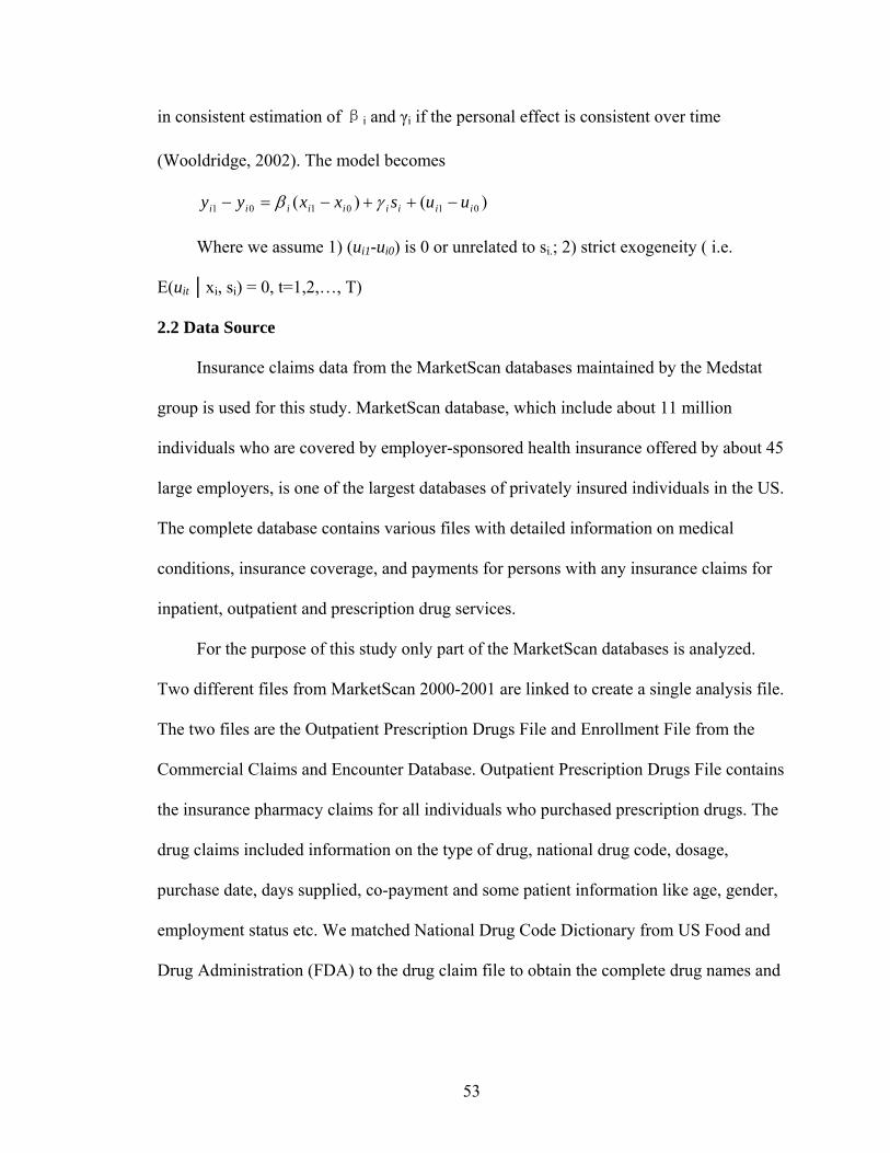
53
in consistent estimation of βi and γi if the personal effect is consistent over time
(Wooldridge, 2002). The model becomes
)()( 010101 iiiiiiiii uusxxyy −++−=− γβ
Where we assume 1) (ui1-ui0) is 0 or unrelated to si.; 2) strict exogeneity ( i.e.
E(uit │xi, si) = 0, t=1,2,…, T)
2.2 Data Source
Insurance claims data from the MarketScan databases maintained by the Medstat
group is used for this study. MarketScan database, which include about 11 million
individuals who are covered by employer-sponsored health insurance offered by about 45
large employers, is one of the largest databases of privately insured individuals in the US.
The complete database contains various files with detailed information on medical
conditions, insurance coverage, and payments for persons with any insurance claims for
inpatient, outpatient and prescription drug services.
For the purpose of this study only part of the MarketScan databases is analyzed.
Two different files from MarketScan 2000-2001 are linked to create a single analysis file.
The two files are the Outpatient Prescription Drugs File and Enrollment File from the
Commercial Claims and Encounter Database. Outpatient Prescription Drugs File contains
the insurance pharmacy claims for all individuals who purchased prescription drugs. The
drug claims included information on the type of drug, national drug code, dosage,
purchase date, days supplied, co-payment and some patient information like age, gender,
employment status etc. We matched National Drug Code Dictionary from US Food and
Drug Administration (FDA) to the drug claim file to obtain the complete drug names and
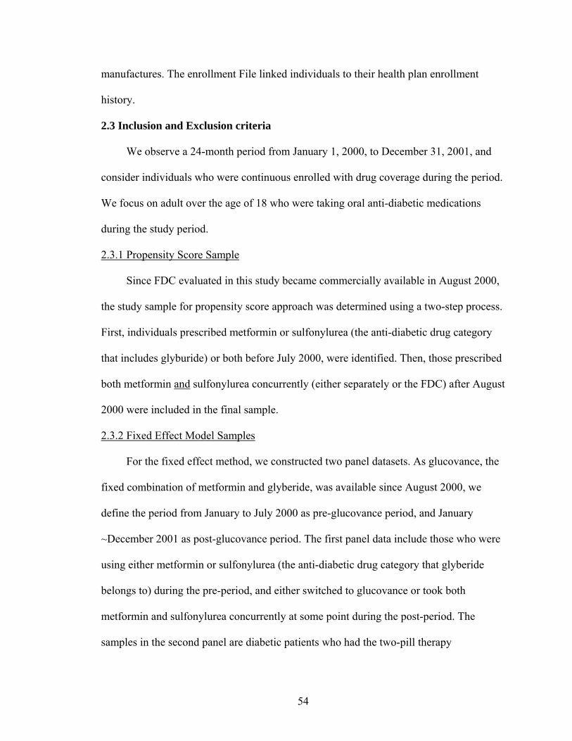
54
manufactures. The enrollment File linked individuals to their health plan enrollment
history.
2.3 Inclusion and Exclusion criteria
We observe a 24-month period from January 1, 2000, to December 31, 2001, and
consider individuals who were continuous enrolled with drug coverage during the period.
We focus on adult over the age of 18 who were taking oral anti-diabetic medications
during the study period.
2.3.1 Propensity Score Sample
Since FDC evaluated in this study became commercially available in August 2000,
the study sample for propensity score approach was determined using a two-step process.
First, individuals prescribed metformin or sulfonylurea (the anti-diabetic drug category
that includes glyburide) or both before July 2000, were identified. Then, those prescribed
both metformin and sulfonylurea concurrently (either separately or the FDC) after August
2000 were included in the final sample.
2.3.2 Fixed Effect Model Samples
For the fixed effect method, we constructed two panel datasets. As glucovance, the
fixed combination of metformin and glyberide, was available since August 2000, we
define the period from January to July 2000 as pre-glucovance period, and January
~December 2001 as post-glucovance period. The first panel data include those who were
using either metformin or sulfonylurea (the anti-diabetic drug category that glyberide
belongs to) during the pre-period, and either switched to glucovance or took both
metformin and sulfonylurea concurrently at some point during the post-period. The
samples in the second panel are diabetic patients who had the two-pill therapy

55
(metformin and sulfonylurea) during the pre-period, and either stayed with the two-pill
therapy or switched to the combination pill. The patient adherence and observable
personal information were measured for both pre- and post-period.
2.4 Measuring Adherence
Drug adherence was measured by Medication Possession Ratio (MPR). As we
described in background section, MPR is defined by the proportion of days on which a
patient had medication available. To calculate the MPR, each day in the follow-up period
was evaluated as ‘covered’ or ‘not covered’ by a prescription fill or refill. If all days
were ‘covered’ by a prescription then adherence was 100%. This MPR algorithm is
similar to the adherence measure described by Bryson and colleagues (2007). The days
on which a patient prescribed two drugs had only one available was included in the
analysis; the MPR was reduced by 50% for these partial adherence days. The continuous
MPR is used in this study.
In propensity score approach, the date of the first claim for metformin and
sulfonylurea (either separately or in the FDC) between September 1, 2000 and December
31, 2001 was defined as that subject’s index date. Each patient was then followed for
180 days after the index claim.
We measure patient adherence for pre and post-FDC periods separately for fixed
effect approach, and follow each patient for 90 days since his/her first metformin or
sulfonylurea or combination of metfomin and sulfonylurea prescription fill during each
period. In addition to MPR measurement, we also measure adherence persistence by
evaluating the gaps between prescription refills in the panel data, as the MPR does not
provide information on the timeliness and consistency of refilling. If the individual did

56
not buy another same-class anti-diabetic prescription within 0.5 times the number of days
supplied by the current prescription after this prescription ran out, he/she would be
considered non-persistence. For example, if a patient filled a 30-day prescription, he
would be allowed 45 days (30+0.5*30) to refill the prescription before being classified as
not persistent. Herein, each patient is also followed for 90 days after his/her first
prescription claim.
2.5 Covariates
To evaluate the likelihood of switching to FDC in propensity score approach,
predictors for the switch to FDC were chosen based on adherence literature:
demographics (age, gender), geographic region (east, north central, west and south),
employment status (hourly worker, union worker, retiree, and dependent), health
insurance characteristics (average drug co-payment, type of plan including fee-for service,
HMO, PPO and POS), health services utilization during the study period, and co-
morbidities. The utilization covariate includes inpatient and outpatient use, number of
medications, the percentage of brand name medications, the days supplied per medication
refill, and the number of refills during the follow-up period. A binary variable was
included to distinguish whether the patient took one or both of the medications
(metformin and/or sulfonylurea) at baseline. Adherence rates in the baseline period prior
to FDC was calculated and included as a predictor of treatment assignment.
For the fixed effect model, the main independent variable is whether the individual
ever used the combination pill glucovance during the post-period. The covariates that
changed during the pre- and post-period are the co-payment by patients, the average days
supply and the number of other anti-diabetic medications except metformin and

57
sulfonylurea used by the patient during the 90-day follow-up. Co-payment is averaged for
each patient over the follow-up period.
3. RESULTS
3.1 Propensity Score Approach Results
3.1.1 Patient Characteristics
A total of 9,170 diabetic patients were prescribed either the FDC or two-pill
regimen in the 180 days follow-up period after glucovance was available. 25% were
prescribed the FDC; the remaining 75% were prescribed concurrent two pill therapy.
Table 1 demonstrates the descriptive patient characteristics for FDC users and two
pill users. Compared to two pill users, FDC users tended to be younger, mainly lived in
the south, and were less likely to be hourly workers or retirees. FDC users, on average,
had higher out of pocket costs for their prescriptions and tended to have a less restricted
heath plan.
FDC users and two pill users did not differ significantly in terms of co-morbidities
and had similar inpatient and outpatient utilization. FDC users were prescribed fewer
medications, tended to use more brand-name drugs, and had shorter days supplied per
prescription, but more refills. Compared to two pill users, FDC users were less likely to
have been prescribed the two component medications before the FDC was available.
Importantly, patients eventually prescribed the FDC had lower adherence rates (measured
as 90-day MPR) during the baseline period. The propensity score approach or fixed effect
would adjust such selection bias and estimate a higher treatment effects.
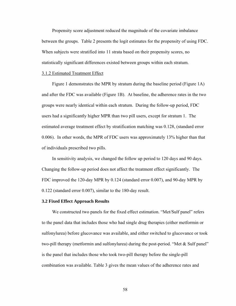
58
Propensity score adjustment reduced the magnitude of the covariate imbalance
between the groups. Table 2 presents the logit estimates for the propensity of using FDC.
When subjects were stratified into 11 strata based on their propensity scores, no
statistically significant differences existed between groups within each stratum.
3.1.2 Estimated Treatment Effect
Figure 1 demonstrates the MPR by stratum during the baseline period (Figure 1A)
and after the FDC was available (Figure 1B). At baseline, the adherence rates in the two
groups were nearly identical within each stratum. During the follow-up period, FDC
users had a significantly higher MPR than two pill users, except for stratum 1. The
estimated average treatment effect by stratification matching was 0.128, (standard error
0.006). In other words, the MPR of FDC users was approximately 13% higher than that
of individuals prescribed two pills.
In sensitivity analysis, we changed the follow up period to 120 days and 90 days.
Changing the follow-up period does not affect the treatment effect significantly. The
FDC improved the 120-day MPR by 0.124 (standard error 0.007), and 90-day MPR by
0.122 (standard error 0.007), similar to the 180-day result.
3.2 Fixed Effect Approach Results
We constructed two panels for the fixed effect estimation. “Met/Sulf panel” refers
to the panel data that includes those who had single drug therapies (either metformin or
sulfonylurea) before glucovance was available, and either switched to glucovance or took
two-pill therapy (metformin and sulfonylurea) during the post-period. “Met & Sulf panel”
is the panel that includes those who took two-pill therapy before the single-pill
combination was available. Table 3 gives the mean values of the adherence rates and
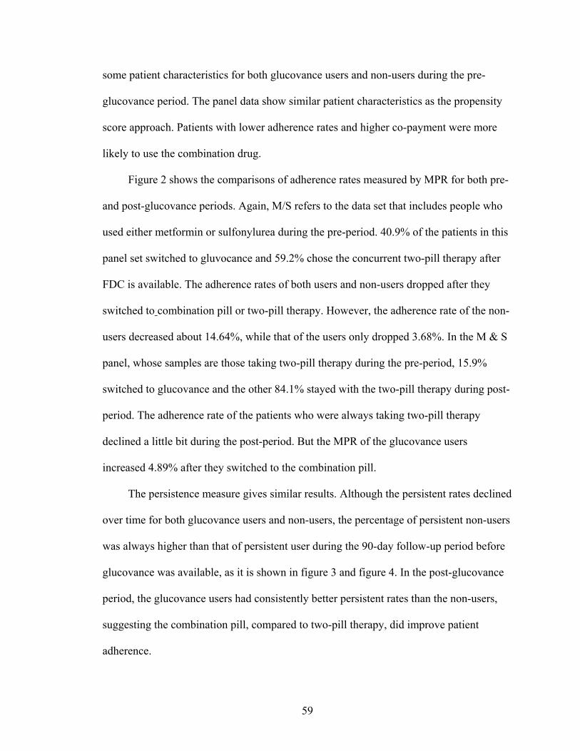
59
some patient characteristics for both glucovance users and non-users during the pre-
glucovance period. The panel data show similar patient characteristics as the propensity
score approach. Patients with lower adherence rates and higher co-payment were more
likely to use the combination drug.
Figure 2 shows the comparisons of adherence rates measured by MPR for both pre-
and post-glucovance periods. Again, M/S refers to the data set that includes people who
used either metformin or sulfonylurea during the pre-period. 40.9% of the patients in this
panel set switched to gluvocance and 59.2% chose the concurrent two-pill therapy after
FDC is available. The adherence rates of both users and non-users dropped after they
switched to combination pill or two-pill therapy. However, the adherence rate of the non-
users decreased about 14.64%, while that of the users only dropped 3.68%. In the M & S
panel, whose samples are those taking two-pill therapy during the pre-period, 15.9%
switched to glucovance and the other 84.1% stayed with the two-pill therapy during post-
period. The adherence rate of the patients who were always taking two-pill therapy
declined a little bit during the post-period. But the MPR of the glucovance users
increased 4.89% after they switched to the combination pill.
The persistence measure gives similar results. Although the persistent rates declined
over time for both glucovance users and non-users, the percentage of persistent non-users
was always higher than that of persistent user during the 90-day follow-up period before
glucovance was available, as it is shown in figure 3 and figure 4. In the post-glucovance
period, the glucovance users had consistently better persistent rates than the non-users,
suggesting the combination pill, compared to two-pill therapy, did improve patient
adherence.

60
The OLS regressions with fixed effects adjust observed and unobserved patient
characteristic that may affect medication adherence, and find the same conclusion (table
4). Compared with the two-pill therapy, glucovance improved patient adherence
measured by MPR by 11.3% for those who used single drug therapy (metformin or
sulfonylurea) during the pre-period, and by 6.5% for two-pill therapy patients. The
combination pill also increased the percentage of persistent patients at the end of 90-day
follow-up by 17.6% in the Met/Sulf panel, and by 14.6% in the Met & Sulf panel.
4. DISCUSSION
Combination drug is not a new concept. But as more and more combination drugs
come to the market as an effort by the drug companies to extend the patent life and
profitability of the key agent in the combination, it is valuable to assess how these drugs
affect patient’s adherence to medication. We used both propensity score and fixed effect
approaches to control for selection bias. Our estimates for both approaches show similar
results: the anti-diabetic FDC drug, glucovance, significantly increased patient adherence
to combination therapy when compared to patients prescribed a two-pill regimen. The
estimated improvement ranges from 6.5-14.6%, depending on the adherence measure and
analytic approach.
The study has some important limitations. First, both propensity score and fixed
effect methods cannot fundamentally solve the non-random assignment bias. If the switch
to the FDC is correlated with unobserved factors whose effects on adherence change over
time, the results might be biased. However, the analysis on FDC users and non users
reveals that FDC users tend to be non-compliant compared to the non users. The

61
traditional OLS analysis might underestimate the FDC effect. Propensity score and fixed
effect approaches both corrected for such selection bias problem. Second, due to data
availability, only short-term effects were measured. Because switching to the FDC likely
involves clinician visit, the importance of good adherence may have been emphasized to
the patient in connection with the switch, which could result in improved adherence.
Therefore, for this and other reasons, the long term durability of the adherence
advantages of FDC drugs is uncertain. Future work could analyze the long-term
adherence trend among FDC users versus non-users when data is available, as long-term
adherence is more important for patients with chromic illness. Third, the generalizability
of these results is limited. The study population included well-insured employees of
large companies. Future studies may need to focus on individuals with less generous
prescription drug coverage. Also, no information was available on length or severity of
disease.
As more than one medication becomes the norm to achieve recommended clinical
endpoints for many chronic diseases, the effect of multiple medications on patient
adherence becomes especially important. Our findings suggest that compared to two pill
therapy, a fixed dose combination can yield important improvements in patient adherence.
In the case where the acquisition costs of a FDC product exceeds the cost of the
individual agents, cost-effectiveness analyses are warranted to determine whether the
clinical advantages attributable to the enhanced adherence are worth the incremental
expenditures. In addition, future work should evaluate the effects of FDC on different
subgroups to identify the groups that would benefit from FDC most. As FDC is usually

62
more expensive than the free dose combinations, it would be valuable to identify the
groups who have, at least, enough adherence gains to offset the extra costs.

63
Table 3.1 Comparison of Covariates for FDC Users and Non-FDC Users
Variables FDC Users
Non-FDC
Users Unadjusted P
Value Demographics Age, year Mean (SD) 52.4 (0.13) 54.4 (0.07) <0.001 18-44 (% of patients) 12.5% 8.5% <0.001 45-54 (% of patients) 38.6% 36.6% 0.115 55-64 (% of patients) 48.6% 52.5% <0.001 65+ (% of patients) 0.3% 1.4% <0.001 Gender(% of male) 55.5% 56.1% 0.345 Region (% of patients) 0.0% 0.0% East 12.8% 23.3% <0.001 North Central 26.1% 26.0% 0.918 South 59.0% 45.7% <0.001 West 2.0% 5.1% <0.001 Employment (% of patients) 0.0% 0.0% Hourly 24.7% 26.9% 0.048 Union 20.0% 19.0% 0.289 Retiree 28.0% 32.1% <0.001 Dependent 0.2% 0.3% 0.279 Health Insurance Drug Co-payment $ Mean (SD) 13.11 (0.18) 9.60 (0.07) <0.001 FFS (% of patients)* 25.7% 21.2% <0.001 HMO(% of patients)* 2.7% 6.9% <0.001 PPO(% of patients)* 27.8% 29.5% 0.134 POS(% of patients)* 43.8% 42.4% 0.737 Health Services Utilization Two-drug users prior to FDC (% of patients)** 32.8% 68.6% <0.001 Adherence rate prior to FDC Mean (SD) 0.833 (0.004) 0.853 (0.002) <0.001 No. of Medications Mean (SD) 6.2 (0.10) 7.1 (0.06) <0.001 % brand-name Medications 94.8% 80.1% <0.001 Average days supply per fill Mean (SD) 41.8 (0.50) 50.4 (0.32) <0.001 # of Refills Mean (SD) 3.4 (0.04) 2.6 (0.02) <0.001 Outpatient encounters Mean (SD)*** 19.6 (0.32) 19.6 (0.21) 0.926 Hospitalized at least once*** 6.2% 6.0% 0.698 Comorbidities Hypertension (% of patients) 53.2% 51.7% 0.233 Heart Failure (% of patients) 5.4% 5.4% 0.980 Depression (% of patients) 18.4% 19.6% 0.249 Propensity Score Mean (SD) 0.505 (0.006) 0.157 (0.002) <0.001 No. of Observations 2275 Note: *FFS is Fee-For-Service, HMO is Health Management Organization, PPO is Preferred Provider Organization, POS is Point Of Service **Two-drug users refers to those who used both metformin and sulfonylurea prior to FDC ***The time frame for inpatient and outpatient encounter is 09/2000~12/2001
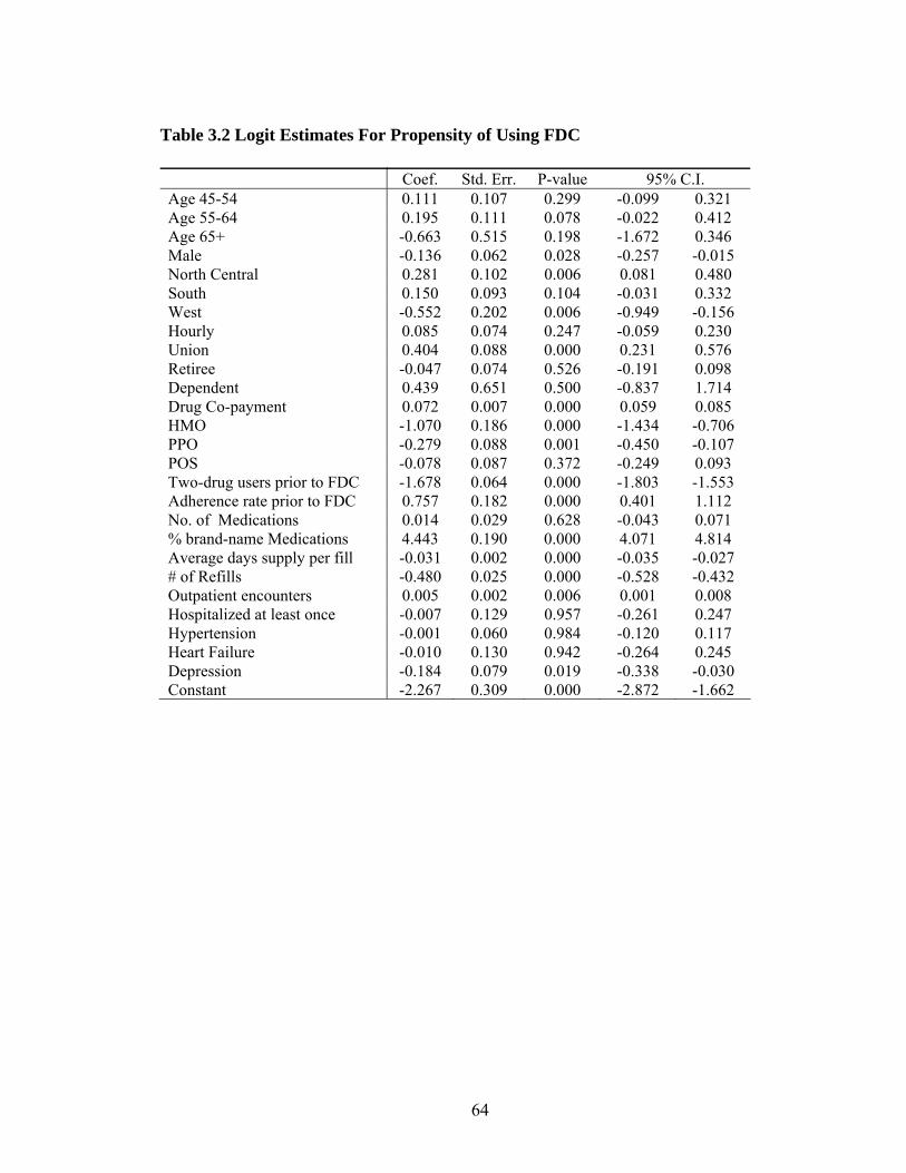
64
Table 3.2 Logit Estimates For Propensity of Using FDC Coef. Std. Err. P-value 95% C.I. Age 45-54 0.111 0.107 0.299 -0.099 0.321 Age 55-64 0.195 0.111 0.078 -0.022 0.412 Age 65+ -0.663 0.515 0.198 -1.672 0.346 Male -0.136 0.062 0.028 -0.257 -0.015 North Central 0.281 0.102 0.006 0.081 0.480 South 0.150 0.093 0.104 -0.031 0.332 West -0.552 0.202 0.006 -0.949 -0.156 Hourly 0.085 0.074 0.247 -0.059 0.230 Union 0.404 0.088 0.000 0.231 0.576 Retiree -0.047 0.074 0.526 -0.191 0.098 Dependent 0.439 0.651 0.500 -0.837 1.714 Drug Co-payment 0.072 0.007 0.000 0.059 0.085 HMO -1.070 0.186 0.000 -1.434 -0.706 PPO -0.279 0.088 0.001 -0.450 -0.107 POS -0.078 0.087 0.372 -0.249 0.093 Two-drug users prior to FDC -1.678 0.064 0.000 -1.803 -1.553 Adherence rate prior to FDC 0.757 0.182 0.000 0.401 1.112 No. of Medications 0.014 0.029 0.628 -0.043 0.071 % brand-name Medications 4.443 0.190 0.000 4.071 4.814 Average days supply per fill -0.031 0.002 0.000 -0.035 -0.027 # of Refills -0.480 0.025 0.000 -0.528 -0.432 Outpatient encounters 0.005 0.002 0.006 0.001 0.008 Hospitalized at least once -0.007 0.129 0.957 -0.261 0.247 Hypertension -0.001 0.060 0.984 -0.120 0.117 Heart Failure -0.010 0.130 0.942 -0.264 0.245 Depression -0.184 0.079 0.019 -0.338 -0.030 Constant -2.267 0.309 0.000 -2.872 -1.662
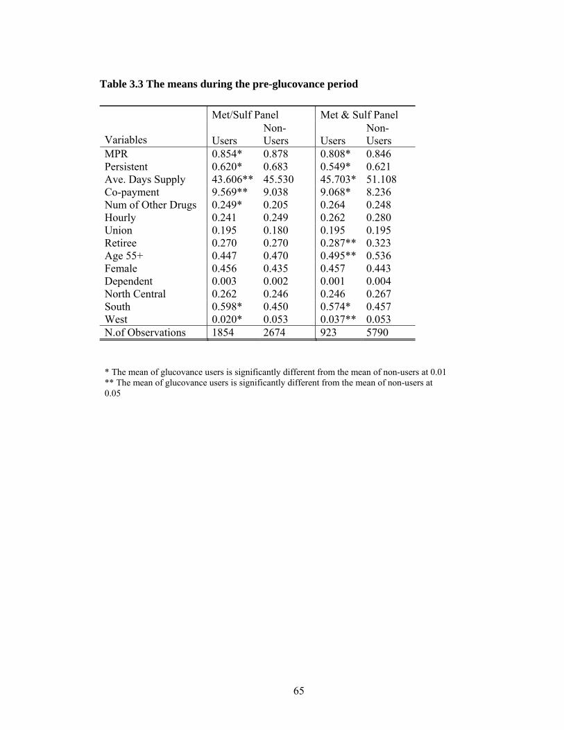
65
Table 3.3 The means during the pre-glucovance period
Met/Sulf Panel Met & Sulf Panel
Variables Users Non-Users Users
Non-Users
MPR 0.854* 0.878 0.808* 0.846 Persistent 0.620* 0.683 0.549* 0.621 Ave. Days Supply 43.606** 45.530 45.703* 51.108 Co-payment 9.569** 9.038 9.068* 8.236 Num of Other Drugs 0.249* 0.205 0.264 0.248 Hourly 0.241 0.249 0.262 0.280 Union 0.195 0.180 0.195 0.195 Retiree 0.270 0.270 0.287** 0.323 Age 55+ 0.447 0.470 0.495** 0.536 Female 0.456 0.435 0.457 0.443 Dependent 0.003 0.002 0.001 0.004 North Central 0.262 0.246 0.246 0.267 South 0.598* 0.450 0.574* 0.457 West 0.020* 0.053 0.037** 0.053 N.of Observations 1854 2674 923 5790 * The mean of glucovance users is significantly different from the mean of non-users at 0.01 ** The mean of glucovance users is significantly different from the mean of non-users at 0.05
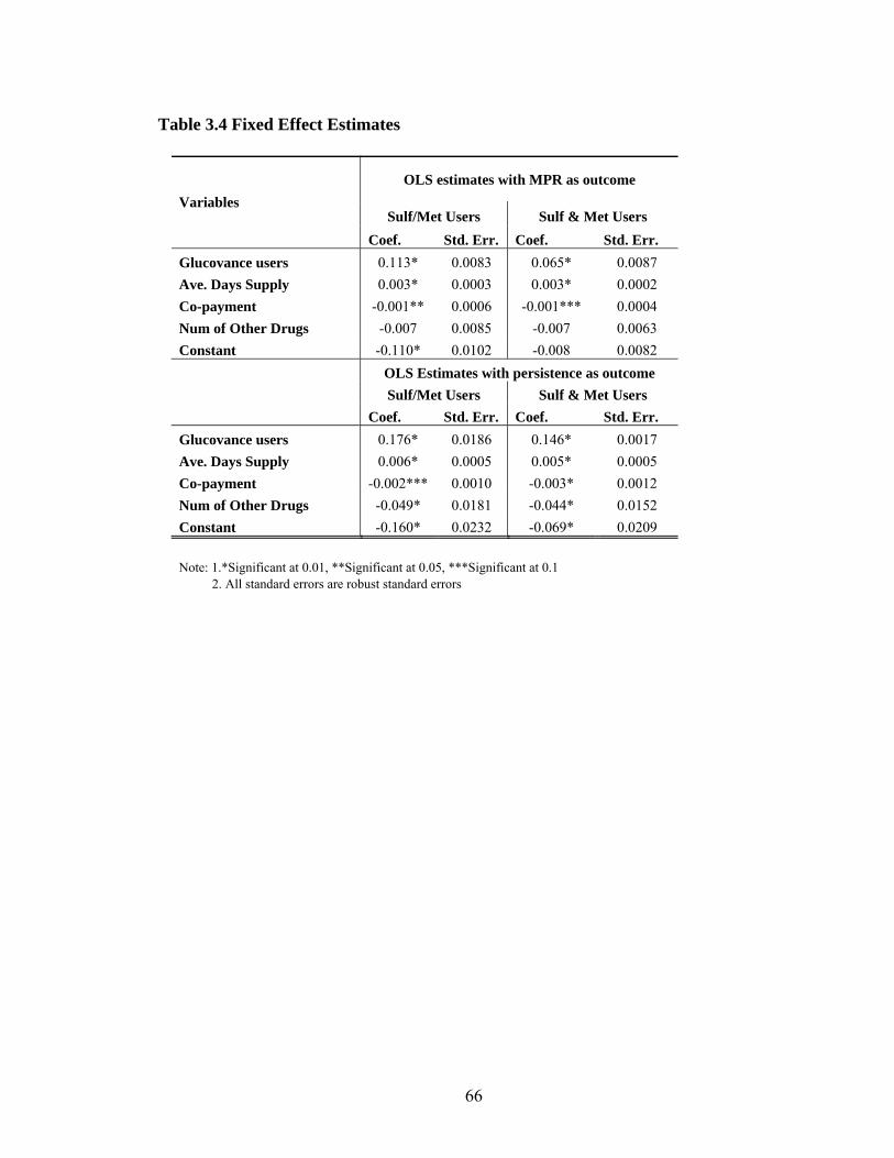
66
Table 3.4 Fixed Effect Estimates
OLS estimates with MPR as outcome
Sulf/Met Users Sulf & Met Users Variables
Coef. Std. Err. Coef. Std. Err. Glucovance users 0.113* 0.0083 0.065* 0.0087 Ave. Days Supply 0.003* 0.0003 0.003* 0.0002 Co-payment -0.001** 0.0006 -0.001*** 0.0004 Num of Other Drugs -0.007 0.0085 -0.007 0.0063 Constant -0.110* 0.0102 -0.008 0.0082 OLS Estimates with persistence as outcome Sulf/Met Users Sulf & Met Users Coef. Std. Err. Coef. Std. Err. Glucovance users 0.176* 0.0186 0.146* 0.0017 Ave. Days Supply 0.006* 0.0005 0.005* 0.0005 Co-payment -0.002*** 0.0010 -0.003* 0.0012 Num of Other Drugs -0.049* 0.0181 -0.044* 0.0152 Constant -0.160* 0.0232 -0.069* 0.0209 Note: 1.*Significant at 0.01, **Significant at 0.05, ***Significant at 0.1 2. All standard errors are robust standard errors

67
Figure 3.1 Medication Possession Ratio by Propensity Score Stratum, Before and After the Availability of the Fixed Dose Combination Product
A. Prior to FDC
0.5
0.55
0.6
0.65
0.7
0.75
0.8
0.85
0.9
0.95
1
1 2 3 4 5 6 7 8 9 10 11Propensity Score Stratum
Medic
ati
on
Poss
ess
ion
Rati
o
Non-FDC Users FDC Users
B. Post FDC
0.5
0.55
0.6
0.65
0.7
0.75
0.8
0.85
0.9
0.95
1
1 2 3 4 5 6 7 8 9 10 11
Propensity Score Stratum
Medic
ati
on
Poss
ess
ion
Rati
o
Non-FDC Users FDC Users

68
Figure 3.2 Panel data Comparison on MPRs
0.65
0.7
0.75
0.8
0.85
0.9
non-users, M/S users, M/S non-users, M&S users, M&S
Prior to FDC Post-FDC
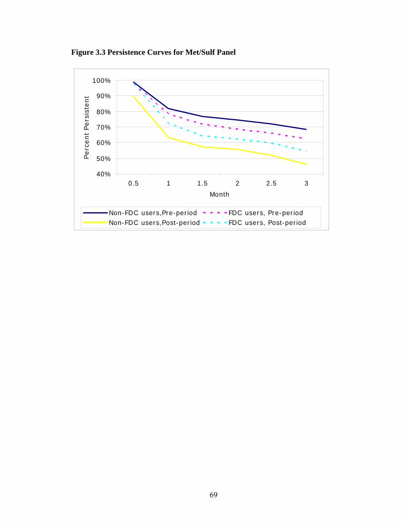
69
Figure 3.3 Persistence Curves for Met/Sulf Panel
40%
50%
60%
70%
80%
90%
100%
0.5 1 1.5 2 2.5 3
Month
Perc
ent
Pers
iste
nt
Non-FDC users,Pre-period FDC users, Pre-periodNon-FDC users,Post-period FDC users, Post-period

70
Figure 3.4 Persistence Curves for Met & Sulf Panel
50%
60%
70%
80%
90%
100%
0.5 1 1.5 2 2.5 3
Month
Perc
ent
Pers
iste
nt
Non-FDC users,Pre-period FDC users, Pre-periodNon-FDC users,Post-period FDC users, Post-period

71
References Avorn, J. et al ‘Persistence of use of lipid-lowering medications: a cross-national study”
JAMA, 1998 Benner, JS et al “Long-term persistence in use of statin therapy in elderly patients” JAMA.
2002 Bloom, BS “Continuation of initial antihypertensive medication after 1 year of therapy”
Clinical Therapeutics, 1998 Blonde, L. “Management of type 2 diabetes: update on new pharmacological options”
Managed Care 2000 supplement Bryson CL, Au DH, Young B, McDonell MB, Finh SD. A Refill Adherence Algorithm
for Multiple Short Intervals to Estimate Refill Compliance (ReComp). Medical Care. 2007; 45(6): 497-504.
Cantrell, C.R., Eaddy, M.T., Shah, M.B., Regan, T.S., Sokol, M.C. Methods for
Evaluating Patient Adherence to Antidepressant Therapy: A Real-World Comparison of Adherence and Economic Outcomes. Medical Care. 2006; 44(4): 300-303.
Catalan, VS et al “Predictor of persistence of use of the novel antidiabetic agent
acarbose” Archives of Internal Medicine, 2001 Christian-Herman, J. et al “Effect of generic-only drug coverage in a Medicare HMO”
Health Affairs, 2004 Cramer, JA et al “How often is medication taken as prescribed?” JAMA, 1989 Crystal, S. et al “The diffusion of innovation in AIDS treatment: zidovudine use in two
New Jersey cohorts” Health Service Research, 1995 Dailey, D. et al “Patient compliance and persistence with antihyperglycemic drug
regimens: evaluation of a Medicaid patient population with type 2 diabetes mellitus.” Clinical Therapeutics, 2001
Degli, EL et al “A retrospective, population-based analysis of persistence with
antihypertensive drug therapy in primary care practice in Italy”. Clinical Therapeutics, 2002
Dehejia, RH and S. Wahba Propensity score-matching methods for nonexperimental
causal studies. Review of Economics and Statistics. 2002; 84(1): 151-161. Detry, et al “Patient compliance and therapeutic coverage: amlodipine vs nifedipine in
the treatment of angina pectoris.” Journal of General Internal Medicine, 1994

72
Dezii, CM “A retrospective study of persistence with single-pill combination therapy vs.
concurrent two-pill therapy in patients with hypertension” Managed Care, 2000 supplement
Dezii, CM et al “Effects of once-daily and twice-daily dosing on adherence with
prescribed Glipizide oral therapy for type 2 diabetes” Southern Medical Journal, 2002
Dor, A. and Encinosa, W. “Does cost sharing affect compliance? The case of prescription
drugs.” NBER working paper, 2004 Ellis, JJ et al “Suboptimal statin adherence and discontinuation in primary and secondary
prevention populations: should we target patients with the most to gain?” Journal of General Internal Medicine, 2004
Fang H., Keane, MP and Silverman D. “Sources of Advantageous Selection: Evidence
from the Medigap Insurance Market” Journal of Political Economy 2008 116(2) Grant, RW et al “Polypharmacy and medication adherence in patients with type 2
diabetes” Diabetes Care, 2003 Gibson, TB et al “The effect of prescription drug cost sharing: a review of the evidence”
The American Journal of Managed Care, 2005 November Leichter, S.B. and Thomas, S. “Combination Medications in Diabetes Care: An
Opportunity that Merits More Attention” Clinical Diabetes, 22(4) 2003 McCombs, J.S., Nichol, M.B., Newman, C.M., Sclar, D.A. The costs of interrupting
antihypertensive drug therapy in a medicaid population. Medical Care. 1994; 32(3): 214-216.
Melikian, C., White, T.J., Vanderplas, A., Dezii, C.M., Chang E. Adherence to oral
antidiabetic therapy in a managed care organization: a comparison of monotherapy, combination therapy, and fixed-dose combination therapy. Clinical Therapeutics. 2002; 24(3): 460-467.
Perkins SM, Tu W, Underhill MG et al. The use of propensity scores in
pharmacoepidemiologic research. Pharmacoepidemiology and Drug Safety. 2000; 9:93-101
Perwien, A. et al “Stimulant treatment patterns and compliance in children and adults
with newly treated attention-deficit/hyperactivity disorder” Journal of Managed Care Pharmacy, 2004
73
Pilote, L. et al “The effects of cost-sharing on essential drug prescriptions, utilization of medical care and outcomes after acute myocardial infarction in elderly patients” CMAJ, 2002
Rosenbaum P.R., Rubin, DB. The central role of the propensity score in observational
studies for causal effects. Biometrika. 1983; 70(1): 41-55. Sikka, R. et al “Estimating medication persistency using administration claims data” The
American Journal of Managed Care, 2005 July Steiner, JF et al “The effect of prescription size on acquisition of maintenance
medications” Journal of General Internal Medicine, 1993 Steiner, JF and Prochazka, AV “The assessment of refill compliance using pharmacy
records: methods, validity and applications” Journal of Clinical Epidemiology, 1997 Vermeire, E., Hearnshaw, H., Van Royen, P and Denekens, J. Patient adherence to
treatment: three decades of research. A comprehensive review. Journal of Clinical Pharmacy and Therapeutics. 2001; 26(5): 331-342.
Wertheimer, A.I., Morrison, A. Combination Drugs: Innovation in Pharmacotherapy.
P&T; 2002, 27(1): 44-49. Wooldridge, J. M. Econometric Analysis of Cross Section and Panel Data. Cambridge,
MA, The MIT Press 2002
74
CHAPTER IV
THE EFFECT OF CO-PAYMENT CHANGE ON PRESCRIPTION
DRUG UTILIZATION-TIER SHIFTING
1. BACKGROUND
Prescription drug costs have been the fastest growing component of health care
spending in the United States during the early 21st century. In 2002, $162 billion was
spent on prescription drugs (a 15% increase from the prior year) and the costs of
prescription drugs are expected to continue rising sharply (Kaiser Family Foundation,
2004). In response, employers and health benefit managers have been increasingly
shifting costs to employees in an attempt to control rising drug expenditures (Dietz 2004;
Robinson 2004). Patient cost-sharing is designed to reduce health care use (Zweifel 2000;
Newhouse 1993) and, empirically, the literature is quite clear that increased medication
co-payments work as desired, leading to a reduction in medication utilization (Ellis et al
2004; Federman et al 2001, Goldman et al 2004; Johnson et al 1997; Piette et al 2004).
The critical issue surrounding medication cost-sharing, though, is whether patients can
determine which drugs are most valuable to their health and then, in turn, whether they
will choose to prioritize their medications accordingly to maximize health outcomes.

75
Unfortunately, the evidence suggests that medication cost-sharing indiscriminately
reduces the use of both excess and essential medications alike (Ellis et al 2004; Federman
et al 2001, Goldman et al 2004; Johnson et al 1997; Piette et al 2004). In turn, growing
evidence suggests that individuals who decrease medication utilization due to out of
pocket (OOP) costs have poorer health outcomes (Johnson et al 1997; Piette et al 2004;
Heisler et al 2004; Schoen et al 2001) and may even incur increases in overall health care
costs (Soumerai, et al 1991).
In response to the growing evidence that ‘one-size fits all’ co-payment harm
patients and may even increase costs, a more nuanced approach to health insurance
benefits design, in which patients’ co-payments are based on the expected clinical benefit
of the prescribed drug(s) rather than their acquisition cost, was proposed (Chernew et al
2000; Fendrick et al 2001). Under this Value Based Insurance Design (VBID) theory, the
more beneficial the medication, the lower the co-payment, thereby effectively realigning
the incentives faced by patients to increase utilization of and adherence to the most
beneficial and valuable prescription medications.
Empirically, it appears that the appeal of such clinically-based benefits has taken
root primarily outside of medicine – in the business world. In an effort to reduce high
cost claims, FORTUNE 500 employer (and self-insurer) Pitney Bowes lowered
medication co-payments for asthma and diabetes medications in 2001 and reported a one
year one million dollar savings in the Wall Street Journal (Hensley 2004). A few other
health plans are experimenting with similar strategies. CIGNA HealthCare offers a four-
tier formulary option it terms the “tiered clinical utility” approach, with “life-saving”
drugs in the lowest co-payment tier and “lifestyle” drugs in the highest co-payment tier

76
(Fendrick 2005). While these clinically sensitive benefit designs hold promise for
improving the quality and value of care, there have been no well designed evaluations,
and certainly no prospective, controlled evaluations, of these more nuanced benefit
designs.
The Focus On Diabetes (FOD) intervention implemented at the University of
Michigan (UM) is the first of its kind designed both to improve the quality of care for
UM employees, and to allow for a rigorous evaluation of such a program’s effectiveness.
Diabetes was chosen as the initial condition because of the improved ability to identify
diabetes through pharmacy claims, and because a detailed assessment in the UM
population identified clear underutilization of evidence-based therapies in employees and
dependents with diabetes. The intervention started from July 1, 2006 and provided all
UM employees and dependents identified as having diabetes with co-payment reductions
for all glycemic agents, anti-hypertensives, lipid lowering agents, and anti-depressants.
One of the important impacts of FOD intervention is patients’ drug utilization
pattern change. Incentive-based or tiered formularies, which provide financial incentives
(i.e. lower co-payments) for enrollees to choose drugs that are preferred by the payer, has
been a popular drug benefit design to curb the increasing costs of prescription drug
(Gabel et al, 2002). Incentive-based formularies are intended to preserve choice for
patients and physicians by providing some level of coverage for most drugs while
encouraging patients and their physicians to select the drugs that are more cost effective
for the plan. The use of incentive-based formularies could also result in increased
bargaining power for plans to negotiate rebates with drug manufactures by promising an
increased volume of prescriptions for the preferred drugs (Frank, 2001)
77
A three-tier formulary, now the most common type and provided to UM employees
and their dependents, requires the lowest co-payments for generic drugs (tier 1), a higher
co-payment for the brand-name drugs that are preferred by the health plan (tier 2), and
the highest co-payments for brand-name drugs that are not preferred by the health plan
(tier 3). The co-payment reductions in FOD intervention were designed to maintain the
underlying incentive structure of the formulary such that generic medications (tier 1) had
larger co-payment reductions than branded medications, and preferred brands (tier 2) had
larger co-payment reductions than tier 3. Specifically, the generic drug co-payment
reduced from $7 to $0 (100%), preferred brand-name drugs from $14 to $7 (50%), and
non-preferred brand-name drugs from $24 to $18 (25%).
How the graded co-payment changes within tiered formulary affect patient tier
utilization pattern has important implication to health plan, as the possible more
utilization on non-preferred mediations could impose unnecessary higher costs to health
plan. Previous studies have found that the adaptation of an incentive-based formulary
and/or increase co-payments resulted in switching to lower tier medications. However it
is not clear whether FOD intervention will result in more non-preferred drug utilization
or not.
Standard economic theory predicts that changes in prices directly affect the relative
quantities of products purchased. Every price change can be decomposed into an income
effect and a substitution effect. The income effect from co-payment reduction may lead to
more consumption of costly drugs as the patients’ budget constraint is relaxed. This
hypothesis will hold if patients believe that the higher tier medications (especially brand
name versus generic drugs) have better quality, and thus prefer them. The substitution
78
effect, on the other hand, may shift the utilization toward lower tiered drugs, since graded
co-payment reductions changed the relative price among drugs in different tiers, and
generic drugs became relatively cheaper than brand-name ones, and non-preferred drugs
are relatively more costly than preferred ones to patients.
Extensive literature has studied relative price change on product selection and some
(Smith DG and Rose LC) found that the use of uniform dollar change induced increased
consumption of the lower priced alternatives given limits of insurance coverage. In
addition, price reduction could increase the amount of utilization among all tiers. That is
patients may start to take more drugs and be more adherent to the treatment regimens.
Although the quantity effect of the co-payment reduction is not evaluated in this study, it
may reduce the income effect from the price reduction. Given the economic theories and
empirical evidence, we would hypothesize that the graded co-payment reduction may
switch patients from higher tier to lower tier.
In this chapter, the effects of the FOD intervention on drug utilizations are evaluated.
Specifically, we examined how changes in co-payment reductions on the targeted drugs
affected patient tier switching within drug class. Non-UM enrollees from the same health
plan provider (M-CARE) serve as control group in the study, as their employers did not
provide such co-payment reductions on these drugs.
The analyses show that the graded co-payment reductions did not change the tier use
on diabetic and anti-hypertensive medications, as most UM patients remained on their
original tier after intervention. However, for the lipid lowering medications and anti-
depressants, the effect of co-payment reduction is not clear, because patent expiration and

79
formulary changes on both UM and control groups accompanied co-payment reductions
during the study period.
The chapter proceeds as follows: In section 2, I describe the empirical methods used,
including FOD intervention details, data source, concurrent drug benefit changes and
statistical analyses. In section 3, I present the empirical results, followed with discussion
of implications, limitation and future work in section 4.
2. EMPIRICAL ANALYSIS
2.1 Focus On Diabetes Intervention
On July 2006, the University of Michigan implemented the Focus On Diabetes (FOD)
intervention, which was designed as a prospective, controlled intervention of targeted co-
payment reductions for high value pharmacotherapies in diabetes. The intervention
population consists of UM active employees and their dependents continuously enrolled
in SXC Health Solutions (the sole pharmacy benefit provider for UM) and M-CARE (the
medical health plan), and identified as diabetic based on at least one pharmacy claim for
diabetic hypoglycemic medications (oral or injectable) or supplies within the 12 months
prior to study initiation.
An educational letter was sent to the entire UM community one month prior to
initiation of the co-payment reductions, which provided information on the general health
benefits of medication adherence, the specific benefits of the drugs selected for
intervention, and a brief description of the impending co-payment reductions. A parallel
letter was sent to the control group (described below) which differed from the UM letter
in that it excluded information about the co-payment reductions (but included all of the

80
same educational content). The two letters also differed in that, while both provided a
phone number for questions (phone staffed by a registered nurse), the letter to UM
employees and dependents also contained a statement allowing individuals to opt out of
or opt into the study.
While the FOD intervention is designed to reduce financial barriers to effective
therapies, it does not preclude the concomitant use of other incentive structures already in
place. Prior to the intervention, UM employed a 3-tiered formulary with co-payments of
$7, $14, and $24 for generic, preferred brand, and non-preferred brand medications,
respectively. This underlying benefit structure remains intact with the value based
benefit overlaid. Further, to maintain incentives to minimize cost (when health remains
unaffected), the intervention lowers co-payments in a graded fashion (tier 1’s co-payment
decreases by 100%, tier 2’s by 50% and tier 3’s by 25%) to a new 3-tiered benefit
structure of $0, $7, and $18 for the medications of interest.
2.2 Control Group
Non-UM enrollees from the same health plan provider M-CARE were identified as
the control population. M-CARE is a large managed care organization in south east
Michigan, and was owned by the University at the time FOD was initiated. The same
pharmacy claims criteria used to identify the UM employees with diabetes (the
intervention group) were used to identify the non-UM managed care enrollees with
diabetes (the control group).
The control group is employees and their dependents from about 170 employers in
south east Michigan. Many of them are relatively small employers, with more than 50%
of them having less than 250 M-CARE enrollees. Although these employers have

81
different prescription drug benefit, they all employed 3-tier formulary with varying co-
payment requirements, and no co-payment change happened among these employers at
the same time as the FOD intervention period. The characteristics of the control group are
presented in the results section.
2.3 Inclusion Criteria
Enrollment files, pharmacy claim data and medical utilization claim data were
obtained from M-CARE. For the purpose of this study, an 18 month period from January
01, 2006 to June 30, 2007 is analyzed (6 months prior to and 1 year after FOD
intervention). Individuals who were continuously enrolled with drug coverage over this
entire period and have at least one diabetic medication claim during the year prior to
intervention are considered. In addition, this study considers tier switching only.
Discontinuation from treatment or uptake is not analyzed here. Therefore only those with
at least one fill of the study drug class prior to the intervention and at least another fill of
the same drug class during the post period are included.
2.4 Drug Class
Focus On Diabetes intervention involved four groups of drug classes: glycemic
(diabetic) agents, anti-hypertensives, lipid lowering agents and anti-depressants. Table 1
presents the four drug class groups, the drug classes within each group and their
corresponding shares in each group. Most of the drug consumptions concentrated in a few
major drug classes. Statins, for example, accounted for 82% of utilization of lipid
lowering agents.
In this study, tier switching is analyzed within drug classes listed in the table 1. That
is if a patient was taking two drugs from the same medication group, she/he is counted

82
twice in the analyses for that drug group. The reason is that although patients may switch
among the drug classes within the same medication group, it is very common that
patients take multiple drugs from different drug classes within the same group, as each of
these drugs works differently to treat conditions and sometimes they are complimentary
to each other. For the treatment of diabetes, for example, patients usually start with one
drug, increase its dose until maximum dosing, and then start another class of drug, either
alone or in combination with the first drug.
2.5 Concurrent Changes to Drug Benefit
Other than FOD intervention, the University of Michigan made some drug formulary
changes during the study period, by moving some brand name drugs from tier 2 to tier 3.
At the same time, formulary changes happened among the employers in the control group
too. Because the control group consists of 170 employers (many of them are small
business), these formulary changes vary across control group patients. All of these might
complicate the tier switching analysis. Table 2 lists all the formulary changes during the
study period among both intervention and control groups. The corresponding market
shares of these drugs are presented in table 1.
In addition, the patents of two major brand-name drugs from Statin and SSRIs/SNRI
drug classes expired around the same time FOD intervention began. Zocor, a Statin agent
produced by Merck, and Zoloft, a SSRI drug produced by Pfizer, lost their patents on
July 23, 2006 and June 30, 2006 respectively. Because generic drugs were available right
after the patent expirations, we may expect a shift from brand name to generic tier among
these two drug classes.
2.6 Analysis
83
In the primary analysis, individuals in the data were sorted into three groups:
(0) Down shifting – individuals who switched to lower formulary tier but using
the same drug class during the post intervention period.
(1) No change – those who remained on their original formulary tier during the
study period
(2) Up shifting – individuals who switched to higher formulary tier but using
the same drug class during post intervention period
Additionally, a secondary outcome was analyzed, which measures the switch to and
from generic tier within each drug class. That is the variable will be 0 if the patient
switched from brand name to generic drug, 1 if the patient remained on brand name or
generic drugs, and 2 if the patient switched from generic to brand name drug. In addition,
if a patient had multiple claims for the same drug class, the latest claims during each
period (pre and post intervention periods) are included in the study.
3. RESULTS
3.1 Population Characteristics
Table 3 presents the study population characteristics and overall tier utilization before
and after FOD intervention for both the intervention group – the University of Michigan
employees and their dependents, and the control group – the non-U of M enrollees in M-
CARE health plan. A total number of 759 UM enrollees and 1491 non-UM enrollees
meet the inclusion criteria. The two groups have similar mean age (50 years old) and
gender distribution (50% female). UM enrollees had a little bit higher number of
84
concurrent medications (5.55 vs 4.96), longer average drug days supply (64 days vs 59
days), and lower average co-payment ($12.68 vs $14.65) before the FOD intervention.
The average co-payment UM enrollees paid after the intervention decreased more
than 50% (from $12.68 to $4.97), while the co-payment for the control group remains
almost unchanged.
The total medication consumption on each tier for both pre and post intervention
periods are also presented in table 3. Before intervention, UM enrollees have higher
consumption of generic and preferred brand name drugs, while non-UM enrollees have
higher percentage on non-preferred brand name drugs. During the post intervention
period, however, both groups have a significant shift to generic drugs (UM group
increased by 10%, and control group increased by 6%). This can be explained by the fact
that two major drugs, Zocor (Statins) and Zoloft (SSRIs), lost their patent almost at the
same time the intervention began. Besides switching to first tier, about 4% of UM drug
utilizations shifted to the highest tier, resulting in relative less consumption of preferred
brand name drugs. The control group, on the other hand, moved in an opposite direction,
with more preferred brand name drug utilization and less tier 3 use.
The preliminary summary of drug tier utilization pattern change reveals that the effect
of FOD intervention is mixed with those of patent expirations and concurrent drug
benefit changes. A detailed drug utilization analysis by medication groups and drug
classes is described in the next section.
3.2 Tier Utilization Patterns By Medication Groups
Figure 1-4 show the tier utilization distributions by medication groups during both pre
and post intervention periods. In diabetic medication group, UM enrollees were almost

85
unaffected by the intervention in terms of tier utilization. Non-UM enrollees had more
preferred brand name diabetic drug utilization during the post period, while their generic
drug use did not change. The formulary change table (table 2) shows that one of
metformin drugs was moved from tier 3 to tier 2, and metformin has about 54% share of
the total diabetic drug consumption (table 1), which explained why the control group
increased their use on preferred diabetic medications. For anti-hypertensives (figure 2),
the tier utilization nearly remained the same after intervention for both treatment and
control group. Although the control group had some formulary change on anti-
hypertensives during the study period (table 2), the number of drugs moving from tier 2
to tier 3 equals the number of drugs from tier 3 to tier 2.
For lipid lowering agents and anti-depressants, however, tier utilization changed
significantly during post-intervention period (figure 3 and 4). These changes are mainly
due to the patent expiration of Zocor (Statins) and Zoloft (SSRIs). UM enrollees had
relatively higher increase in generic lipid lowering agents utilization, while the control
group had higher increase in generic anti-depressants use. For UM enrollees, 4 Statin
drugs moved from tier 2 to tier 3 during the post intervention period, but there is no
change in formulary tier of anti-depressants. As a result, UM enrollees increased both tier
1 and tier 3 consumptions of lipid lowering drugs and decreased preferred brand name
use, while just replaced some of the tier 2 use with generic drugs in anti-depressants
group. Among the non-UM group, patent expirations were mixed with more complex
formulary change on lipid lowering agents (table 2). Consequently, the non-UM group
increased both tier 1 and tier 2 utilization of lipid lowering drugs and reduced non-
preferred brand name consumption.

86
The analyses on individual tier shifting by medication groups show similar results as
the figures (table 4 and 5). Utilizations by formulary tiers on diabetic drugs and anti-
hypertensives did not change among UM enrollees after the FOD intervention, as
majority of the patients remained no change (diabetic drugs 99.17%, anti-hypertensives
96%). Among non-UM enrollees, drug formulary changes led to slightly higher tier
shifting rates on these two medication groups.
Among lipid lowering agents and anti-depressants, fewer patients remained on the
same drug tiers during post intervention period. 30% UM enrollees shifted to lower tier
of lipid lower agents and 23.3% moved to higher tier. The combination of Zocor patent
expiration and formulary changes toward moving more tier 3 drugs to tier 2 resulted in
47% of non-UM enrollees shifting to lower tiers in this drug group. For anti-depressants,
about 25% UM enrollees and 20% non-UM enrollees changed their tiers. And more
patients in UM group (7.4%) moved to higher formulary tier than the non-UM group
(2.25%).
Separate analyses on Statin and SSRIs/SNRIs are presented in table 6, as these two
drug classes had patent expiration during the study period. 38.9% of UM patients moved
to generic Statin, compared to 23.7% of non-UM patients. However, non-UM enrollees
had higher rates (22.65%) of shifting to generic SSRIs than the UM treatment group
(18%). The co-payment reductions on UM side cannot explain the different relative
shifting rates in these two drug classes. Rather, the formulary changes provide some
explanations. UM moved more brand-name Statin drugs from tier 2 to tier 3 to encourage
the use of generic drugs after Zocor lost its patent, while non-UM employers moved
Zoloft to tier 3 after its patent expired to encourage the use of generic version.
87
4. DISCUSSION
Focus On Diabetes is a drug benefit experiment conducted on the University of
Michigan employees and their dependents. The FOD experiment reduced drug co-
payments of four types of prescription medications for diabetic patients. This study
evaluates how the co-payment reduction affected patient formulary tier utilization
patterns. The analyses show that the graded co-payment reductions did not change the tier
use on diabetic and anti-hypertensive medications, as most people remained on their
original tier after intervention. However, for the lipid lowering medications and anti-
depressants, the effect of co-payment reduction is not clear, due to the fact that patent
expiration and formulary changes on both UM and control groups accompanied co-
payment reductions during the study period. Patent expirations of Zocor (Simvastatin)
and Zoloft (Sertraline HCL) resulted in significant shifting from brand-name to generic
drugs. Moving brand-name drugs from tier 2 to tier 3 encouraged the use of generic drugs.
This study has several important limitations. First, the effects of concurrent formulary
changes are mixed with that of co-payment reductions. It is hard to evaluate the pure
graded co-payment reductions on tier shifting behavior, especially for the use of lipid
lowering agents and anti-depressants. Second, the control group consists of 170
employers. The ongoing changes to their drug benefits are not unanimous and the
heterogeneity may make the control group less comparable to the intervention group.
Future work may use UM patients themselves as control, by comparing their tier
utilization on non-FOD intervention drugs to the FOD intervention drugs. In addition, the
University of Michigan enrollees are well insured population. The average co-payment

88
UM patients paid before FOD intervention was less than $13. The generalizability of
these results is limited. Future studies may need to focus on individuals with less
generous drug benefit, as patients with high co-payments are more sensitive to the benefit
change.
In conclusion, this study found that graded co-payment reductions had little effect on
patient tier switching. Neither income effect nor price effect dominated in the drug price
reduction. Instead, the availability of new generic drugs after the patents of brand-name
drugs expired and drug formulary changes had significant impact on tier shifting.
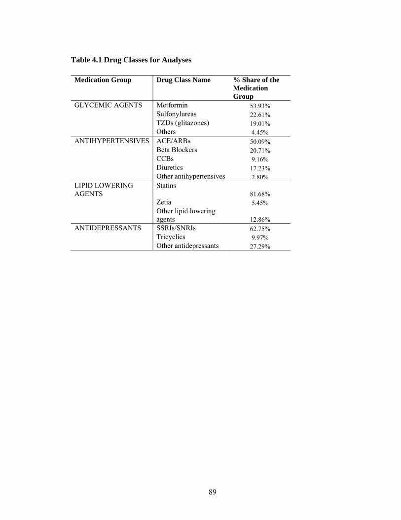
89
Table 4.1 Drug Classes for Analyses Medication Group Drug Class Name % Share of the
Medication Group
GLYCEMIC AGENTS Metformin 53.93% Sulfonylureas 22.61% TZDs (glitazones) 19.01% Others 4.45% ANTIHYPERTENSIVES ACE/ARBs 50.09% Beta Blockers 20.71% CCBs 9.16% Diuretics 17.23% Other antihypertensives 2.80% LIPID LOWERING AGENTS
Statins 81.68%
Zetia 5.45% Other lipid lowering
agents 12.86% ANTIDEPRESSANTS SSRIs/SNRIs 62.75% Tricyclics 9.97% Other antidepressants 27.29%
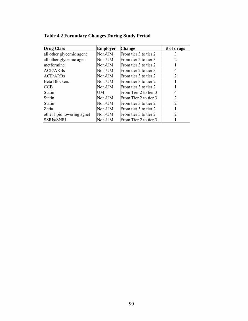
90
Table 4.2 Formulary Changes During Study Period Drug Class Employer Change # of drugs all other glycemic agent Non-UM From tier 3 to tier 2 3 all other glycemic agent Non-UM From tier 2 to tier 3 2 metformine Non-UM From tier 3 to tier 2 1 ACE/ARBs Non-UM From tier 2 to tier 3 4 ACE/ARBs Non-UM From tier 3 to tier 2 2 Beta Blockers Non-UM From tier 3 to tier 2 1 CCB Non-UM From tier 3 to tier 2 1 Statin UM From Tier 2 to tier 3 4 Statin Non-UM From Tier 2 to tier 3 2 Statin Non-UM From tier 3 to tier 2 2 Zetia Non-UM From tier 3 to tier 2 1 other lipid lowering agnet Non-UM From tier 3 to tier 2 2 SSRIs/SNRI Non-UM From Tier 2 to tier 3 1
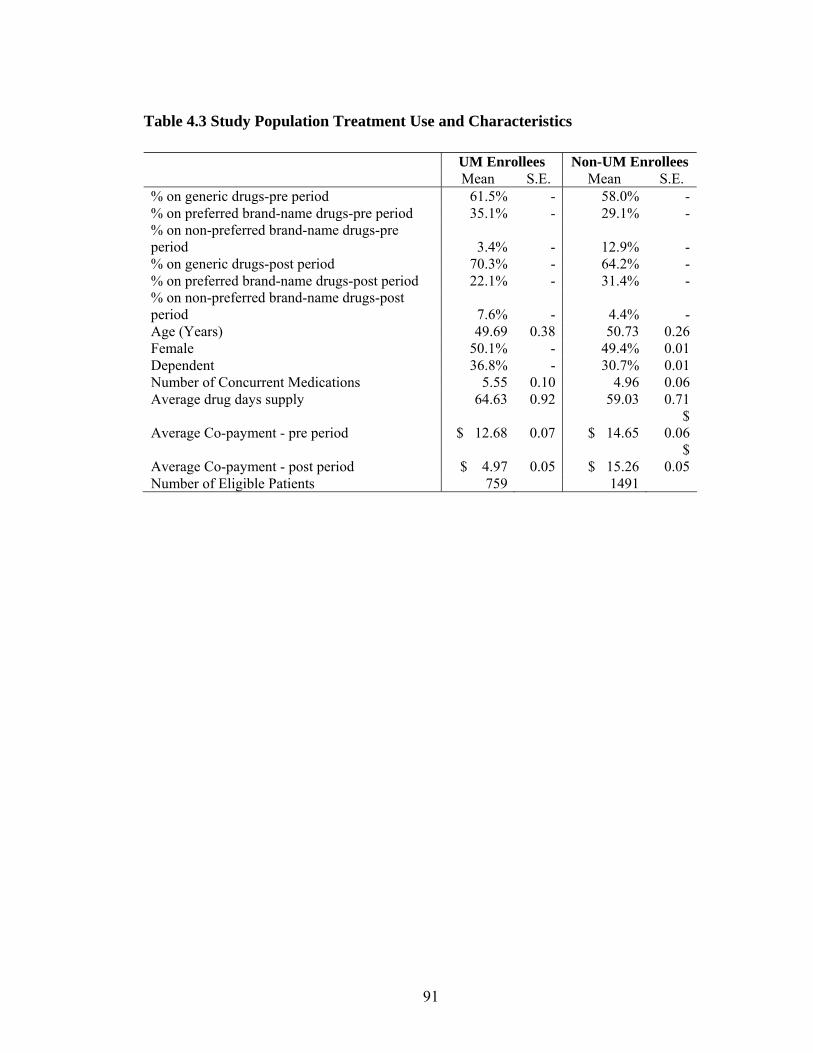
91
Table 4.3 Study Population Treatment Use and Characteristics UM Enrollees Non-UM Enrollees Mean S.E. Mean S.E. % on generic drugs-pre period 61.5% - 58.0% -% on preferred brand-name drugs-pre period 35.1% - 29.1% -% on non-preferred brand-name drugs-pre period 3.4% - 12.9% -% on generic drugs-post period 70.3% - 64.2% -% on preferred brand-name drugs-post period 22.1% - 31.4% -% on non-preferred brand-name drugs-post period 7.6% - 4.4% -Age (Years) 49.69 0.38 50.73 0.26Female 50.1% - 49.4% 0.01Dependent 36.8% - 30.7% 0.01Number of Concurrent Medications 5.55 0.10 4.96 0.06Average drug days supply 64.63 0.92 59.03 0.71
Average Co-payment - pre period $ 12.68
0.07 $ 14.65 $
0.06
Average Co-payment - post period $ 4.97 0.05 $ 15.26 $
0.05 Number of Eligible Patients 759 1491
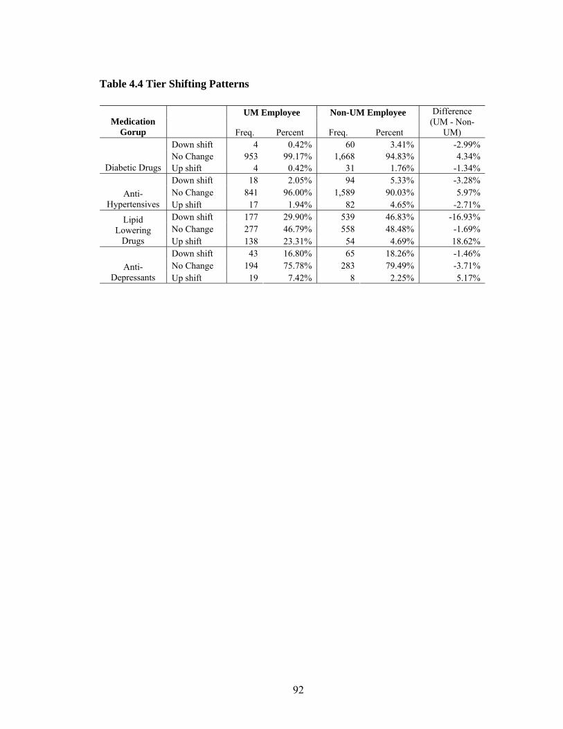
92
Table 4.4 Tier Shifting Patterns
UM Employee Non-UM Employee Medication
Gorup Freq. Percent Freq. Percent
Difference (UM - Non-
UM) Down shift 4 0.42% 60 3.41% -2.99% No Change 953 99.17% 1,668 94.83% 4.34%
Diabetic Drugs Up shift 4 0.42% 31 1.76% -1.34% Down shift 18 2.05% 94 5.33% -3.28% No Change 841 96.00% 1,589 90.03% 5.97% Anti-
Hypertensives Up shift 17 1.94% 82 4.65% -2.71% Down shift 177 29.90% 539 46.83% -16.93% No Change 277 46.79% 558 48.48% -1.69%
Lipid Lowering
Drugs Up shift 138 23.31% 54 4.69% 18.62% Down shift 43 16.80% 65 18.26% -1.46% No Change 194 75.78% 283 79.49% -3.71% Anti-
Depressants Up shift 19 7.42% 8 2.25% 5.17%
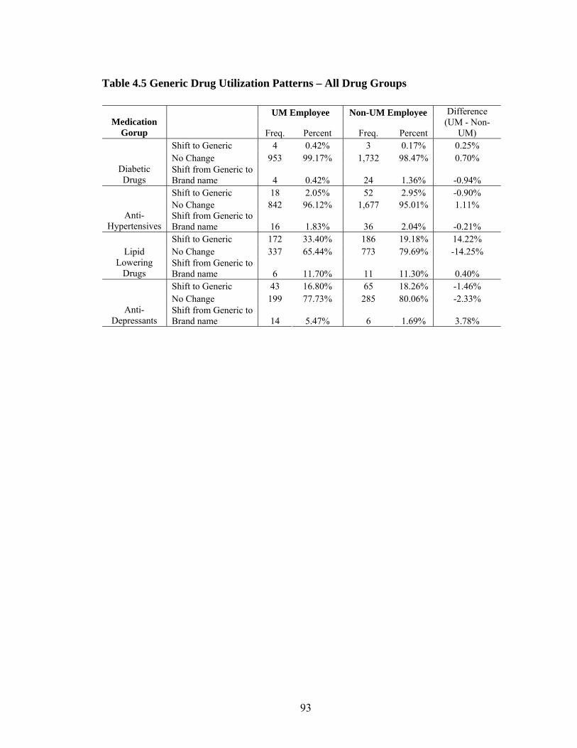
93
Table 4.5 Generic Drug Utilization Patterns – All Drug Groups
UM Employee Non-UM Employee Medication
Gorup Freq. Percent Freq. Percent
Difference (UM - Non-
UM) Shift to Generic 4 0.42% 3 0.17% 0.25% No Change 953 99.17% 1,732 98.47% 0.70%
Diabetic Drugs
Shift from Generic to Brand name 4 0.42% 24 1.36% -0.94% Shift to Generic 18 2.05% 52 2.95% -0.90% No Change 842 96.12% 1,677 95.01% 1.11%
Anti-Hypertensives
Shift from Generic to Brand name 16 1.83% 36 2.04% -0.21% Shift to Generic 172 33.40% 186 19.18% 14.22% No Change 337 65.44% 773 79.69% -14.25% Lipid
Lowering Drugs
Shift from Generic to Brand name 6 11.70% 11 11.30% 0.40% Shift to Generic 43 16.80% 65 18.26% -1.46% No Change 199 77.73% 285 80.06% -2.33%
Anti-Depressants
Shift from Generic to Brand name 14 5.47% 6 1.69% 3.78%
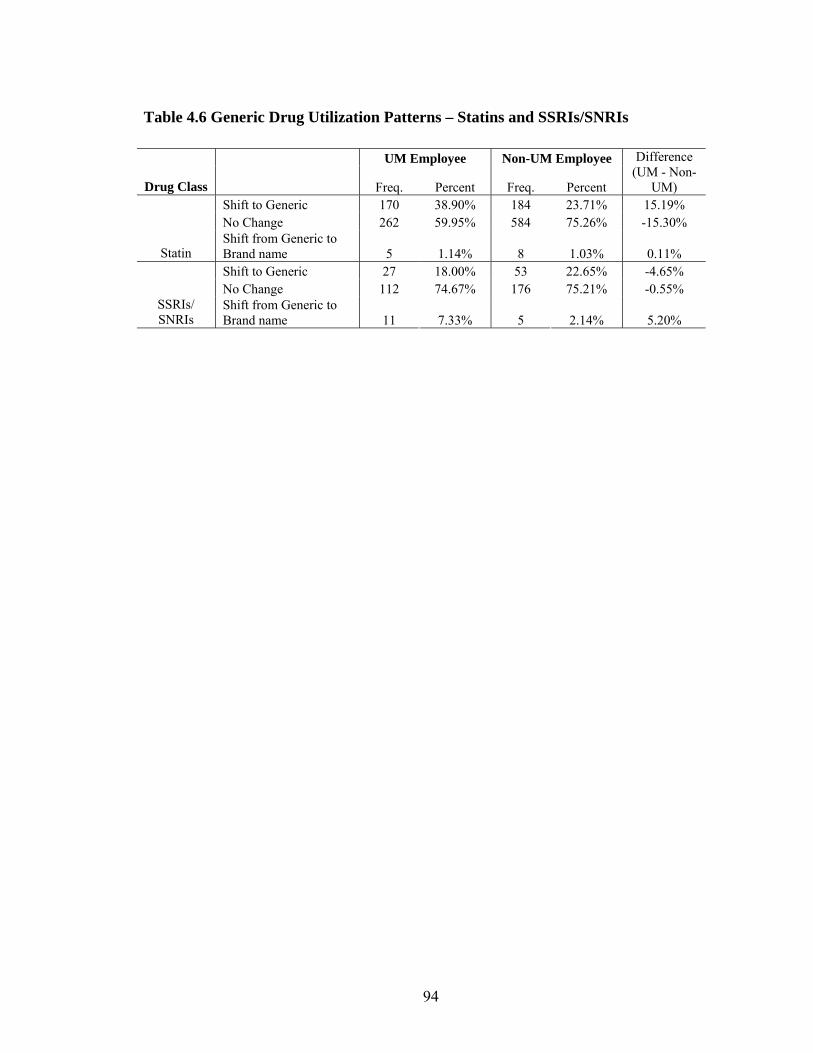
94
Table 4.6 Generic Drug Utilization Patterns – Statins and SSRIs/SNRIs
UM Employee Non-UM Employee
Drug Class Freq. Percent Freq. Percent
Difference (UM - Non-
UM) Shift to Generic 170 38.90% 184 23.71% 15.19% No Change 262 59.95% 584 75.26% -15.30%
Statin Shift from Generic to Brand name 5 1.14% 8 1.03% 0.11% Shift to Generic 27 18.00% 53 22.65% -4.65% No Change 112 74.67% 176 75.21% -0.55%
SSRIs/ SNRIs
Shift from Generic to Brand name 11 7.33% 5 2.14% 5.20%
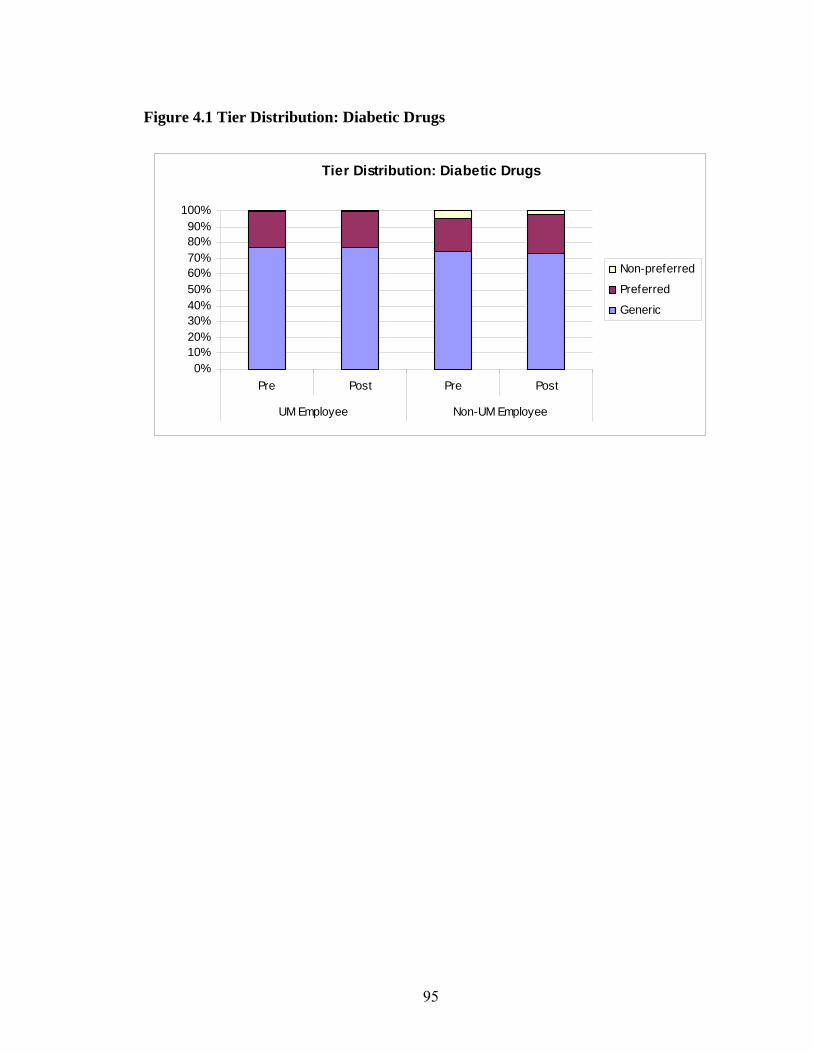
95
Figure 4.1 Tier Distribution: Diabetic Drugs
Tier Distribution: Diabetic Drugs
0%10%20%30%40%50%60%70%80%90%
100%
Pre Post Pre Post
UM Employee Non-UM Employee
Non-preferred
Preferred
Generic
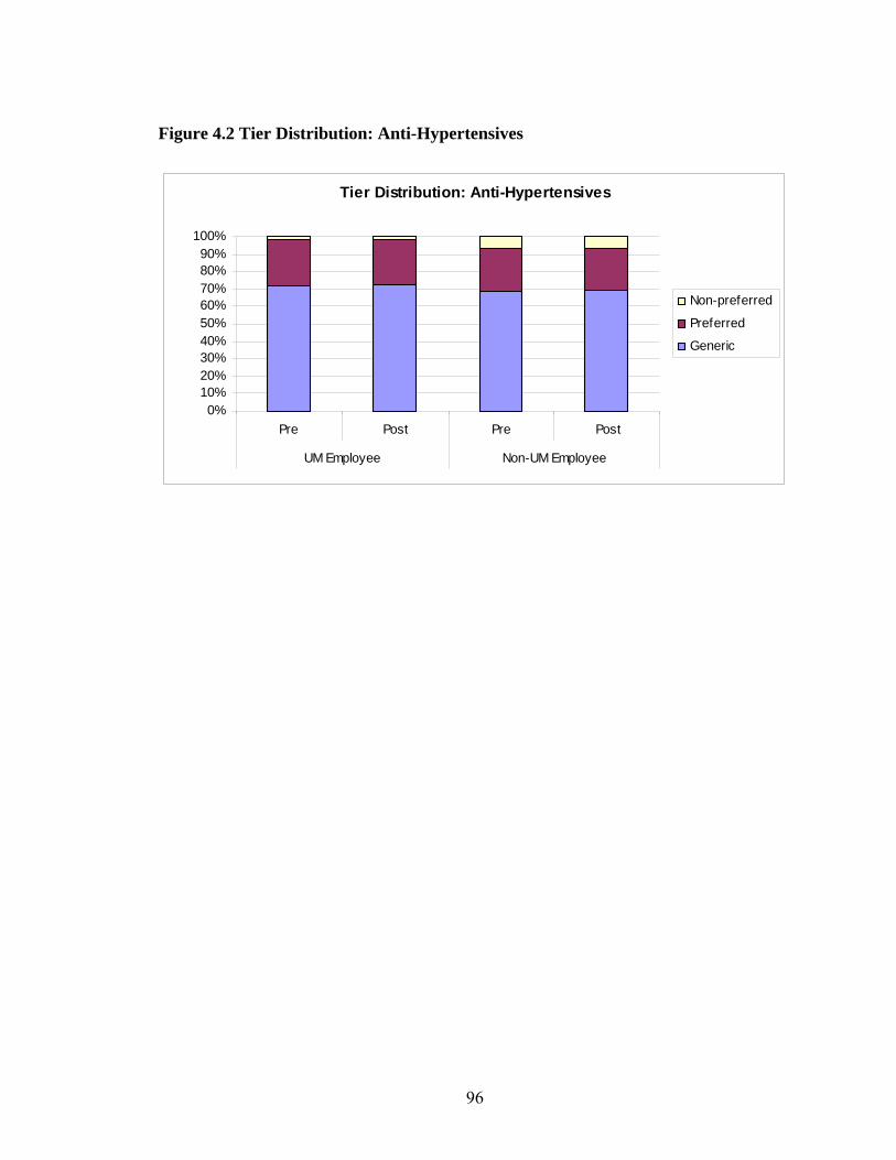
96
Figure 4.2 Tier Distribution: Anti-Hypertensives
Tier Distribution: Anti-Hypertensives
0%10%20%30%40%50%60%70%80%90%
100%
Pre Post Pre Post
UM Employee Non-UM Employee
Non-preferred
Preferred
Generic
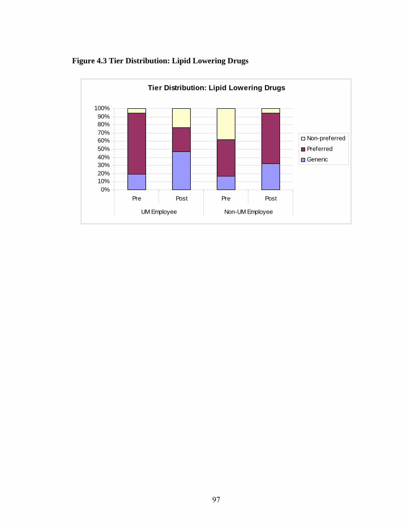
97
Figure 4.3 Tier Distribution: Lipid Lowering Drugs
Tier Distribution: Lipid Lowering Drugs
0%10%20%30%40%50%60%70%80%90%
100%
Pre Post Pre Post
UM Employee Non-UM Employee
Non-preferred
Preferred
Generic
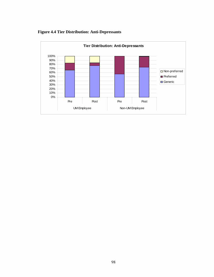
98
Figure 4.4 Tier Distribution: Anti-Depressants
Tier Distribution: Anti-Depressants
0%10%20%30%40%50%60%70%80%90%
100%
Pre Post Pre Post
UM Employee Non-UM Employee
Non-preferred
Preferred
Generic
99
References
Chernew, ME; Encinosa WE; Hirth RA “Optimal health insurance: the case of observable, severe illness” Journal of Health Economics 2000 19(5): p. 585-609
Dietz, E., “Trend in employer-provided prescription drug coverage.” Monthly Labor
Review, 2004. 127(8): p. 37-45. Ellis, J.J., et al., “Suboptimal statin adherence and discontinuation in primary and
secondary prevention populations. Should we target patients with the most to gain?” J Gen Intern Med, 2004. 19(6): p. 638-645.
Federman, A.D., et al., “Supplemental insurance and use of effective cardiovascular
drugs among elderly Medicare beneficiaries with coronary heart disease.” JAMA, 2001. 286(14): p. 1732-1739.
Fendrick, A.M., et al., “A benefit-based copay for prescription drugs: patient contribution
based on total benefits, not on drug acquisition cost”. Am J Manag Care, 2001. 7: p. 861-867.
Fendrick, A.M., “Payers raise the bar by lowering barriers to medications for chronically
ill enrollees.” Drug Benefit News, 2005. 6(7): p. 1-3. Frank, R. “Prescription drug prices: why do some pay more than others do?” Health
Affair 2001 20(2): 115-28 Gabel J., Levitt L, Holve E, et al “ Job-based health benefits in 2002: some important
trends.” Health Affair 2002 21(5):143-51 Goldman, D.P., et al., “Pharmacy benefits and the use of drugs by the chronically ill.”
JAMA, 2004. 291: p. 2344-2350. Heisler, M., et al., “The health effects of restricting prescription medication use because
of cost.” Med Care, 2004. 42(7): p. 626-634. Schoen, M.D., et al., “Impact of the cost of prescription drugs on clinical outcomes in
indigent patients with heart disease.” Pharmacotherapy, 2001. 21(12): p. 1455-1463. Hensley, S., “From 'one size fits all' to tailored co-payments” Wall Street Journal. 2004:
New York City, NY. Johnson, R.E., et al., “The Impact of Increasing Patient Prescription Drug Cost Sharing
on Therapeutic Classes of Drugs Received and on the Health Status of Elderly HMO Members.” Health Serv Res, 1997. 32(1): p. 103-122.
100
Kaiser Family Foundation. “Prescription drug trends (fact sheet).” 2004 [cited 2005 August 7]; Available from: http://www.kff.org/rxdrugs/
Newhouse, J., and the Insurance Experiment Group, “Free for All? Lessons from the
RAND Health Insurance Experiment.” 1993, Cambridge, MA: Harvard University Press. 489.
. Piette, J.D., et al., “Health insurance status, cost-related medication underuse, and
outcomes among diabetes patients in three systems of care.” Med care, 2004. 42: p. 102-109.
Robinson, J.C., “Reinvention of health insurance in the consumer era.” JAMA, 2004.
291(15): p. 1880-1886. Soumerai, S.B., et al., “Effects of Medicaid drug-payment limits on admission to
hospitals and nursing homes.” New England Journal of Medicine, 1991. 325(15): p. 1072-1077.
Zweifel, P. and W.G. Manning, “Moral hazard and consumer incentives in health care.”,
in Handbook of Health Economics, A.J. Culyer and J.P. Newhouse, Editors. 2000, Elsevier: New York City
101
CHAPTER V
CONCLUSIONS
Increased demand for long-term care services and rising prescription drug costs has
attracted growing concerns from health care researchers and policy makers. The goals of
this dissertation are to improve our understandings on long-term care insurance market
and on patient prescription drug utilization.
The cost of long-term care is a concern not only for individuals, but for the public, as
Medicaid and Medicare pay for the majority of the long-term care services. Policymakers
are pursuing a number of initiatives to promote private LTC insurance coverage.
However, some existing theories have provided less support for the efficacy of public
policies by suggesting that the lack of rationale to protect asset may counteract any
incentives created by policies (Pauly, 1990; Zweifel and Struwe 1998). Chapter II of this
dissertation explores whether lack of incentive to protect asset can explain the limited
private long-term care insurance market.
The state partnership programs allow individuals who buy long-term care insurance
policies under the program to protect a certain amount of their assets and become eligible
for Medicaid after they exhaust their policy benefits. Using difference in difference
method, I compare the change in LTC insurance coverage for the partnership states with
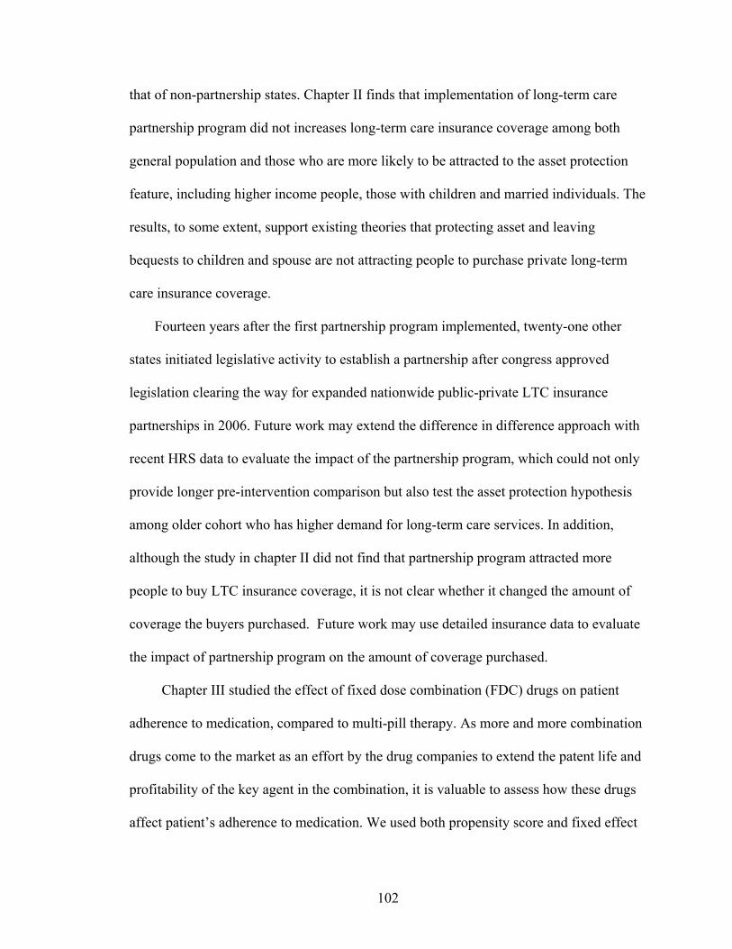
102
that of non-partnership states. Chapter II finds that implementation of long-term care
partnership program did not increases long-term care insurance coverage among both
general population and those who are more likely to be attracted to the asset protection
feature, including higher income people, those with children and married individuals. The
results, to some extent, support existing theories that protecting asset and leaving
bequests to children and spouse are not attracting people to purchase private long-term
care insurance coverage.
Fourteen years after the first partnership program implemented, twenty-one other
states initiated legislative activity to establish a partnership after congress approved
legislation clearing the way for expanded nationwide public-private LTC insurance
partnerships in 2006. Future work may extend the difference in difference approach with
recent HRS data to evaluate the impact of the partnership program, which could not only
provide longer pre-intervention comparison but also test the asset protection hypothesis
among older cohort who has higher demand for long-term care services. In addition,
although the study in chapter II did not find that partnership program attracted more
people to buy LTC insurance coverage, it is not clear whether it changed the amount of
coverage the buyers purchased. Future work may use detailed insurance data to evaluate
the impact of partnership program on the amount of coverage purchased.
Chapter III studied the effect of fixed dose combination (FDC) drugs on patient
adherence to medication, compared to multi-pill therapy. As more and more combination
drugs come to the market as an effort by the drug companies to extend the patent life and
profitability of the key agent in the combination, it is valuable to assess how these drugs
affect patient’s adherence to medication. We used both propensity score and fixed effect
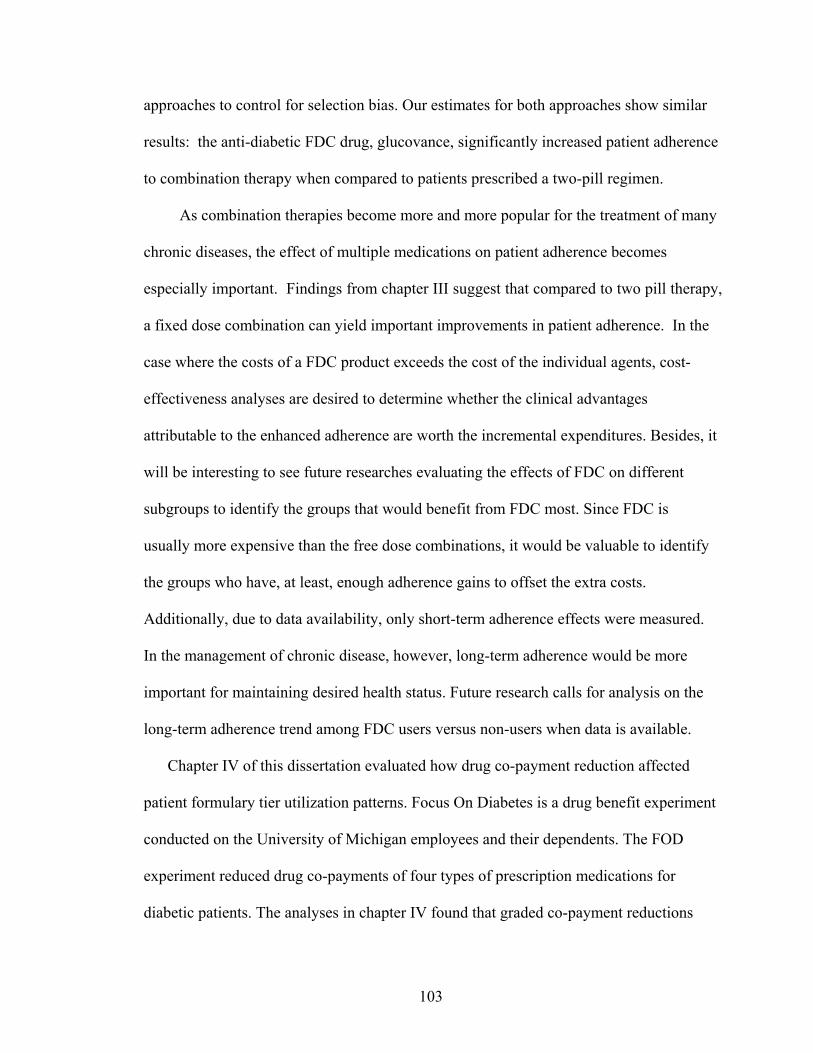
103
approaches to control for selection bias. Our estimates for both approaches show similar
results: the anti-diabetic FDC drug, glucovance, significantly increased patient adherence
to combination therapy when compared to patients prescribed a two-pill regimen.
As combination therapies become more and more popular for the treatment of many
chronic diseases, the effect of multiple medications on patient adherence becomes
especially important. Findings from chapter III suggest that compared to two pill therapy,
a fixed dose combination can yield important improvements in patient adherence. In the
case where the costs of a FDC product exceeds the cost of the individual agents, cost-
effectiveness analyses are desired to determine whether the clinical advantages
attributable to the enhanced adherence are worth the incremental expenditures. Besides, it
will be interesting to see future researches evaluating the effects of FDC on different
subgroups to identify the groups that would benefit from FDC most. Since FDC is
usually more expensive than the free dose combinations, it would be valuable to identify
the groups who have, at least, enough adherence gains to offset the extra costs.
Additionally, due to data availability, only short-term adherence effects were measured.
In the management of chronic disease, however, long-term adherence would be more
important for maintaining desired health status. Future research calls for analysis on the
long-term adherence trend among FDC users versus non-users when data is available.
Chapter IV of this dissertation evaluated how drug co-payment reduction affected
patient formulary tier utilization patterns. Focus On Diabetes is a drug benefit experiment
conducted on the University of Michigan employees and their dependents. The FOD
experiment reduced drug co-payments of four types of prescription medications for
diabetic patients. The analyses in chapter IV found that graded co-payment reductions
104
had little effect on patient tier switching. Neither income effect nor price effect
dominated in the drug price reduction. Instead, the availability of new generic drugs after
the patents of brand-name drugs expired and drug formulary changes had significant
impact on tier shifting. The study is limited by its selection of control group, which
consists of more than 100 employers. The ongoing changes to their drug benefits are not
unanimous and the heterogeneity may make the control group less comparable to the
intervention group. Future work could use UM patients themselves as control, by
comparing their tier utilization on non-FOD intervention drugs to the FOD intervention
drugs.