three-dimensional static and dynamic reactor calculations

1)K &Gooo55

im Risø-R-496

09

Three-dimensional Static and Dynamic Reactor Calculations by the Nodal Expansion Method Brian Christensen

Risø National Laboratory, DK-4000 Roskilde, Denmark May 1985

RISØ-R-496

THREE-DIMENSIONAL STATIC AND DYNAMIC REACTOR CALCULATIONS

BY THE NODAL EXPANSION METHOD

Brian Christensen

This report is written for partial fulfilment of a Ph.D. degree.

Abstract. This report reviews various method for the calculation

of the neutron-flux- and power distribution in an nuclear reac

tor. The nodal expansion method (NEM) is especially described in

much detail. The nodal expansion method solves the diffusion

equation. In this method the reactor core is divided into nodes,

typically 10 to 20 cm in each direction, and the average flux i;

each node is calculated. To obtain the coupling between the

nodes the local flux inside each node is expressed by use of a

polynomial expansion. The expansion is one-dimensional, so inside

each node such three expansions occur. To calculate the expansion

coefficients it is necessary that the polynomial expansion is a

solution to the one-dimensional diffusion equation. When the one-

dimensional diffusion equation is established a term with the

transversal leakage occur, and this term is expanded after the

same polynomials. The resulting equation system with the expan

sion coefficients as the unknowns is solved with weighted resi

dual technique.

(Continued next page)

May 1985

Risø National Laboratory, DK-4000 Roskilde, Denmark

The nodal expansion method is built into a computer program

(also called NEM), which is divided into two parts, one part for

steady-state calculations and one part for dynamic calculations.

It is possible to take advantage of symmetry properties of the

reactor core. The program is very flexible with regard to the

number of energy groups, the node size, the flux expansion order

and the transverse leakage expansion order. The boundary of the

core is described by albedos. The proqram and input to it are

described.

The program is tested on a number of examples extending from

small theoretical ones up to realistic reactor cores. Many cal

culations are done on the we11known IAEA benchmark case. The cal

culations have tested the accuracy and the computing time for

various node sizes and polynomial expansions. In the dynamic ex

amples various strategies for variation of the time step-length

have been tested.

INIS-Descriptors; COMPUTERIZED SIMULATION; N CODES; NEUTRON PLUX;

POLYNOMIALS; POWER DISTRIBUTION; REACTOR CORES; REACTOR KINETICS;

SERIES EXPANSION; THREE-DIMENSIONAL CALCULATIONS

ISBN 87-550-1169-1

ISSN 0106-2840

Grafisk Service Center, Risø 1985

CONTENTS

Page

NOMENCLATURE 5

1. INTRODUCTION 9

2. METHODS FOR THREE-DIMENSIONAL FLUX CALCULATIONS 11

2.1. Finite-difference Methods 13

2.2. Flux-s/nthesis Methods 16

2.3. Finite-element Methods 18

2.4. The Response-matrix Kethod 19

2.5. Nodal Methods 20

2.6. Conclusion 25

3. THEORY POR THE NODAL EXPANSION METHOD 26

3.1. Basic theory for NEM 26

3.2. Stationary equations 38

3.3. Higher-order approximations 39

3.4. Time-dependent theory 49

4. PROGRAMMING 54

4.1. The steady-state main program 55

4.2. Steady-state calculation 59

4.3. Steady-state input and initialization 64

4.4. The calculation of incoming currents 68

4.5. Generation of A-coefficients 69

4.6. Inner iterations 71

4.7. Refinement 71

4.8. Dynamic main program 72

5. EXAMPLES 77

5.1. The IAEA-2D benchmark 78

5.2. The I ABA-3D benchmark 87

5.3. The Biblis-2D benchmark 88 5.4. A typical Westinghouse F.'R 94

5. Infinite slab reactor aodel 103

5.6. The THIGL two-diaensional seed-blanket reactor

kinetics aodel 107

5.7. The LHNLNR transient proble« Ill

5.8. The LRABWR two-diaensional benchaark 115

5.9. The LRABNR three-diaensional benchaark 122

6. CONCLUSION 123

REFERENCES 125

APPENDIX A. Basisfunctions 129

APPENDIX B. Bxaaples 134

APPENDIX C. Solutions 149

APPENDIX D. Input description 171

APPENDIX B. Input examples 187

APPENDIX P. Output exaaples 196

NOMENCLATURE

Symbol Dimension Meaning

A - find coefficient, A-coefficients

A - coefficient Matrix

A* en surface area of node m

perpendicular on x

B - coefficient matrix

B CM'1 right side in the equation systea

for determination of the higher-order

coefficients

Bz en" the buckling

c - expansion coefficients for the one-

dinensional flux

Cj cm concentration of delayed neutrons in

family i

d cm extrapolation distance

d - differentiation

Dg cm diffusion coefficient in group g

D - coefficient matrix

E - coefficient matrix

P - coefficient matrix

F - normalization factor

g - energy group

G - number of energy groups

G - coefficient matrix

I - number of delayed neutron families

j cm"2 s"* currents

J cm~2 s"1 current matrix

K - coefficient matrix in the equation

system for determination of the

higher-order coefficients

L cm'1 transverse leakage

N - expansion orde-

- 6 -

expansion polynomial

coupling Matrix

point vector

tine

arbitrary coordinate


neutron velocity

node volune


x-coordinate

y-coordinate

z-coordinate

albedo

fraction of delayed neutrons in

fanily i

relaxation paraneter

elenents in ganna natrix

ganna natrix

delta, difference, differential

operator

X - eigenvalue

Xj en decay constant

A - nornalization constant

v - average nunber of neutrons

produced in a fission

one-dinensional distribution of

delayed neutrons

cross section

flux in group g at point r to

tine t

flux in group g in node n to tine t

enission spectrun

average one-dinensional flux

coupling coefficients

relaxation paraneter

nabla, Laplacian operator

I*

p

r t

u v v

V

w

X

y 2

a

»i

Y

Y

r A

• -

cn s

cn cn

cn s -

cn3

cn cn cn

cn -

-

-

-

-

_

C

z • g ( r , t )

•g ( t ) X

• u u 7

cn-3

en"' en"2 s"1

c." 2 s ' 1

-

cn"2 s~* -

-

_

Indieies

- 7 -

a absorption (cross section)

d delayed (fission spectrum)

f fission (cross section)

g energy group

i delayed neutron family

1 left (current)

n expansion polynomial order

p prompt (fission spectrum)

r removal (cross section)

r right (current)

s scattering (cross section)

s arbitrary direction - left or right

t total (cross section)

u arbitrary coordinate - x,y,z

Superscripts

i delayed neutron family

in incoming

m node m

r inner iteration number

s outer interation number

out outgoing

negative direction

positive direction

- 9 -

1. INTRODUCTION

The idea of this project is to calculate the three-dimensional

power distribution in a nuclear power reactor when the geo

metric and material constants of the reactor are known. During

the last twenty years scientists the world over have tried to

calculate power distributions and multiplication factors, keff,

for nuclear reactors. Many different methods have been devel

oped with unique advantages and drawbacks. Some computer codes

calculate only steady-state problems and others are restricted

to two-dimensional problems.

There have been great advances not only in the calculacional

methods, but also in the power of the computers themselves.

Problems which took hours of computer time twenty years ago,

today can be managed in a few seconds. It also means that prob

lems which were formerly solved by complicated iteration pro

cesses now are solved by direct and perhaps much simpler

methods.

On the other hand, the computer work has not been redused. In

earlier years the problems were two-dimensional, but today they

are four-dimensional (three-dimensional dynamic problems) which

increases the calculational work by several orders of magnitude.

In Chapter 2 I have tried to summarize and compare some of the

methods which are described in the literature.

The great effort to calculate the power distribution and other

properties of a reactor are made because it is very important

to be able to predict the behaviour of a real reactor before it

is placed into operation. In the design phase the calculation is

especially important in order to understand the subcritical and

supercritical behaviour of the reactor.

Under normal operating conditions the most economical control

rod adjustments and fuel distribution can be simulated and the

- 10 -

reactor made to conform to the model. Burnup can be simulated

and an optimum fuel management strategy proposed. Furthermoret

with a good overall power distribution calculation, it is essen

tial to be able to predict fuel failures.

Another important area is to simulate the reactor under abnormal

conditions, e.g. a control rod ejection. Tn such cases very

severe power transients occur which could have serious effects

on the reactor such as local high-temperature rises. The conse

quences of such an accident have to be simulated to check

whether or not the safety system would be able to handle the

situation.

A computer code for simulation of a reactor core consists of

two nearly distinct parts, which interfere with each other,

but in the programming phase they can be considered independent.

The first one is the neutronic part, which calculates the neutron

flux distribution, the power generation, criticality factors,

etc., and it is this part of the code this report treats. The

second part is the hydraulic one, which treats the heat transport

out of the core and calculates the temperature distribution.

This part will not be treated here, except for a single example

with feedback from the hydraulics.

Today the Energy Technology Department at Risø National Labora

tory bases its overall calculations mainly on the two codes ANTI

(Larsen, 1980), (Nielsen and Larsen, 1980) and NOTAM (Schougaard,

1979). The ANTI-program treats PWR's in both steady state and

dynamic, and NOTAM is able to treat BWR's steady state. Both

codes have their neutronic parts based on the methods used in

ANDYCAP (Babala, Bech and Haugset, 1971) and their results are

not quite as accurate as desired. The accuracy of their results

is rather dependent on the actual problem and also on some em

pirical constants, which often have to be estimated from other

simpler calculations.

Therefore, this work has been initiated with the object of

comparing different methods from the literature and finally im

plementing one at Risø National Laboratory, which is more ac-

- 11 -

curate and preferably quicker than the existing codes. In Chap

ter 2 I have tried to summarize existing methods and in Chapter

3 the theory of what is called the nodal expansion method is

outlined. Chapter 4 describes some of the finer points in the

programming, and in Chapter 5 the program has been tested on

various benchmarks.

2. METHODS POR THREE-DIMENSIONAL FLUX CALCULATIONS

Ever since the appearance of the first computers in the fifties,

calculations on nuclear reactors have been performed. Much prog

ress both in computers and their methodology has been made in

the last thirty years and the codes are now very quick and also

very accurate in most cases. One could argue that the develop

ment of computers with larger and larger memories, such as

CRAY-1 and Cyber-205, could render superfluous further prog

ress in the codes, but this is wrong. At first, the larger com

puters merely encourage scientists to calculate larger problems;

however, power companies and the local power stations perhaps

have access only to smaller computers or even mini-computers.

In this chapter some of the methods for flux calculations are

described very briefly and an attempt is made to summarize the

advantages and disadvantages of the methods. It can be very dif

ficult to compare the different methods, but some of the ques

tions that could be taken into consideration are:

How effective is the method?

How flexible is the method?

Could an error analysis on the result be made?

Is a good theoretical basis for the method available?

Does the solution converge to the exact solution of the

continuous problem for mesh refinement?

- 12 -

Is the method reliable?

Is the method user friendly with respect to inclusion of

feedback effects?

Not all these questions can be answered for the methods, e.g. It

is nearly always impossible or in any case very difficult to

perform an error analysis. It is also difficult to compare the

accuracy and speed of various methods, because different com

puters are used, where calculating times cannot be compared

directly. Besides, one method may be able to handle one problem

very well (it may be optimized to that problem), while it is

hardly able to handle another.

The method that is described below is mainly based on diffusion

theory and the diffusion equation:

1 d* 7 • DV<fr - it . f + s - — • — (2.1)

v dt

For very accurate calculations Boltzmann's transport equation is

a better starting point, but until now and wit* the available

computers, it is too large a task for three-dimensional overall

calculations.

The different methods can be divided roughly into five categor

ies:

1. Finite-Difference methods (FDM)

2. Flux-synthesis methods (FSM)

3. Finite-element methods (FEM)

4. Response-matrix methods (RMM)

5. Nodal methods (NM)

where the main difference is the independent variables. Finite-

difference methods and flux-synthesis methods use point fluxes,

while finite-element methods use expansion coefficients. In the

response-matrix methods the primary variables are the partial

currents, and in the nodal methods they are the average node

fluxes. Some methods can combine more of the above-mentioned

methodd and it can be difficult to classify them.

- i3 -

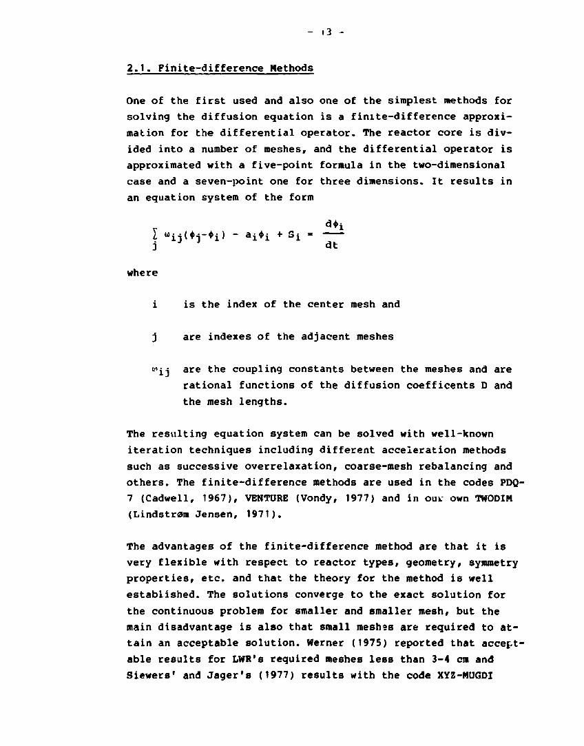
2.1. Finite-difference Methods

One of the first used and also one of the simplest methods for

solving the diffusion equation is a finite-difference approxi

mation for the differential operator. The reactor core is div

ided into a number of meshes, and the differential operator is

approximated with a five-point formula in the two-dimensional

case and a seven-point one for three dimensions. It results in

an equation system of the form

I «ii(*j-*i) " «i*i + Si = j dt

where

i is the index of the center mesh and

j are indexes of the adjacent meshes

("ij are the coupling constants between the meshes and are

rational functions of the diffusion coefficents D and

the mesh lengths.

The resulting equation system can be solved with well-known

iteration techniques including different acceleration methods

such as successive overrelaxation, coarse-mesh rebalancing and

others. The finite-difference methods are used in the codes PDQ-

7 (Cadwell, 1967), VENTURE (Vondy, 1977) and in out own TWODIM

(Lindstrøm Jensen, 1971).

The advantages of the finite-difference method are that it is

very flexible with respect to reactor types, geometry, symmetry

properties, etc. and that the theory for the method is well

established. The solutions converge to the exact solution for

the continuous problem for smaller and smaller mesh, but the

main disadvantage is also that small meshas are required to at

tain an acceptable solution. Werner (1975) reported that accept

able results for LWR's required meshes less than 3-4 cm and

Siewers* and Jager's (1977) results with the code XYZ-MUGDI

- 14 -

showed that the mesh-size should be less than 1.5 cm to produce

reliable results.

With such small mesh sizes the FDM is practically useless for

large three-dimensional calculations, because of the enormous

number of unknowns. On the other hand, the method is good as

reference code, because of the well-founded theory and also be

cause the local flux-distribution is directly attained.

2.1.1. The Coarse Mesh Finite-difference Method HI III • I! -••II«— y » • • 1 MM — m ^ I | — ^ ^ — P ^ ^ ^ ^ M HI — — ^ - ^ ^ ^ —

The finite-difference method can be improved by using a higher-

order approximation for the differential operator, e.g. a nine-

point formula in the two-dimensional case. This gives a coupling

to both the neighbour meshes and the next neighbour mefhes. In

theory this should be a better approximation, but for practical

calculations there are no great advantages with a higher-order

formula.

Another attempt to improve the finite-difference method has been

made by Børresen (1981). He uses the simplest FDM together with

two additional approximations

Di ' Dj 1 -— / D£ • / D T

Di + Dj 2

and

1-a • = a • *i • I *i-j

6 j where

a is a constant

• i is the node average flux

• ij is the flux on the interface between node i and j

- 15 -

With these two approximations the number of variables to be

stored is much smaller than for a conventional FDM and with the

tunable parameter a, the method can use meshes of assembly-size

or half assembly-size.

Siewers and Jager (1977) reported that their code ROSI, which is

based on the same theory, produces accurate results for mesh

sizes in the range of 3 to 10 cm. Børresen uses the method in

the code PRESTO and it is reported to be extremely fast and

rather accurate.

One of the disadvantages of the method is that it uses an

empirically determined constant a, which has to be calculated

by other methods, when a new problem shall be solved. Secondly,

the theoretical background for the method is poor.

2.1.2. The Flux-expansion Method

A higher-order coarse mesh FDM, which is described by Langenbuch

et. al. (1977a), uses a method much like finite-element tech

niques. The reactor is assumed to be composed of rectangular

mesh boxes and the fluxes inside each box are approximated by

polynomials in the x, y, and z direction. The polynomials

Gx " ax * *x + bx ' *2 + cx * 5x + ••••

where the independent variables are expressed in dimensionless

mesh-centered variables, defined in terms of the mesh spacings h

x - xi *x -

hxi

are used in the flux approximations.

The fluxes inside each mesh are approximated in one of two ways,

either the separable Sum-method

• fx,y,z) - •ijjj • (1+Gx+Gy+Gz)

- 16 -

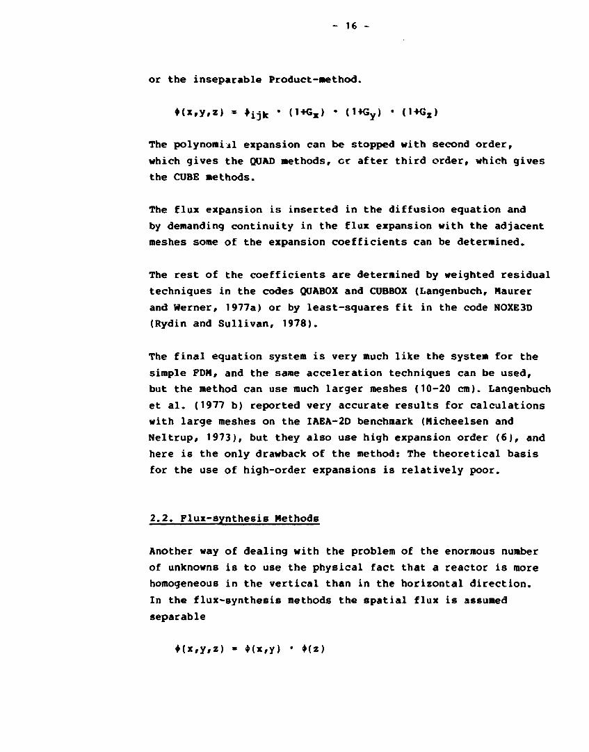
or the inseparable Product-method.

• UrYr*) » •ijjc ' (1+GX> * O+Gy) * (1*5 2 )

The polynomial expansion can be stopped with second order,

which gives the QUAD methods, cr after third order, which gives

the CUBE methods.

The flux expansion is inserted in the diffusion equation and

by demanding continuity in the flux expansion with the adjacent

meshes some of the expansion coefficients can be determined.

The rest of the coefficients are determined by weighted residual

techniques in the codes QOABOX and CUBBOX (Langenbuch, Naurer

and Werner, 1977a) or by least-squares fit in the code N0XB3D

(Rydin and Sullivan, 1978).

The final equation system is very much like the system for the

simple FDM, and the same acceleration techniques can be used,

but the method can use much larger meshes (10-20 cm). Langenbuch

et al. (1977 b) reported very accurate results for calculations

with large meshes on the IAEA-2D benchmark (Nicheeisen and

Neltrup, 1973), but they also use high expansion order (6), and

here is the only drawback of the method: The theoretical basis

for the use of high-order expansions is relatively poor.

2.2. Flux-synthesis Methods

Another way of dealing with the problem of the enormous number

of unknowns is to use the physical fact that a reactor is more

homogeneous in the vertical than in the horizontal direction.

In the flux-synthesis methods the spatial flux is assumed

separable

•(x,y,z) * *(x,y) • *(z)

- 17 -

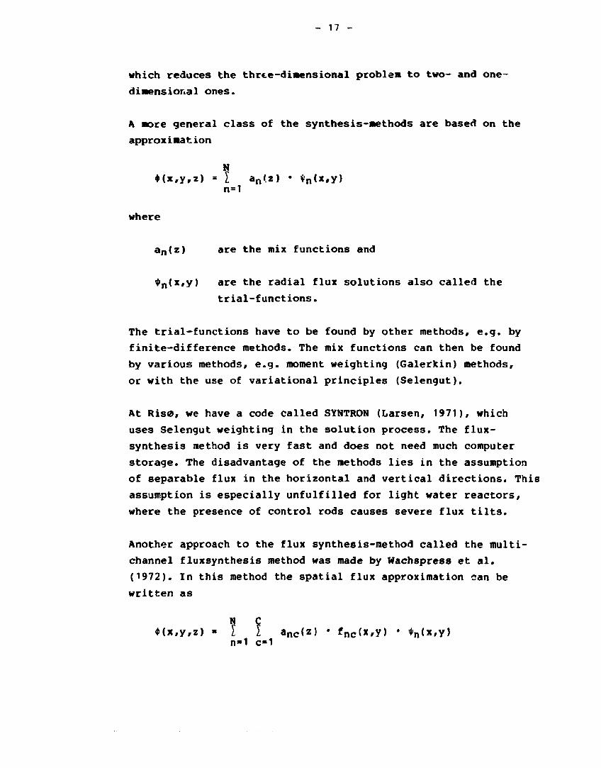
which reduces the three-dimensional problem to two- and one-

dimensional ones.

A more general class of the synthesis-methods are based on the

approximation

N <Mx,y,z) = I an(z) • *n(x,y)

n=1

where

an(z) are the mix functions and

•n(x'v) a r e t n e radial flux solutions also called the

trial-functions.

The trial-functions have to be found by other methods, e.g. by

finite-difference methods. The mix functions can then be found

by various methods, e.g. moment weighting (Galerkin) methods,

or with the use of variational principles (Selengut).

At Risø, we have a code called SYNTRON (Larsen, 1971), which

uses Selengut weighting in the solution process. The flux-

synthesis method is very fast and does not need much computer

storage. The disadvantage of the methods lies in the assumption

of separable flux in the horizontal and vertical directions. This

assumption is especially unfulfilled for light water reactors,

where the presence of control rods causes severe flux tilts.

Another approach to the flux synthesis-method called the multi

channel fluxsynthesis method was made by Wachspress et al.

(1972). In this method the spatial flux approximation can be

written as

*(x,y,z) » I I anc(z) • fnc(x,y) • *n(x,y) n*1 c*1

- 18 -

which differs fro« the preceding one by the additional SUBS over

channels (c for channels) and the set of multichannel basis-

functions fnc(x,y), which permit some modulation of the original

expansion functions. This approximation is able to simulate the

reactor in more detail, but it also requires a user who knows a

great deal about the problem if reliable solutions should be

obtained. The user has to find good tiial functions as well as

choose appropriate channels for the calculation.

2.3. Finite-element Methods

The finite-element technique is well known from other fields of

engineering, particularly structural mechanics, «.nd the methods

are now also applied to reactor physics. The basis idea is to

divide the reactor into meshes called elements, then expand the

flux inside each mesh in terms of piecewise polynomials, and

consider the expansion coefficients as the primary variables.

Continuity conditions along the interfacing of neighbouring

elements give the equations for the unknown coefficients.

With the use of piecewise polynomials, also called basisfunc

tions, it is possible to obtain good approximations of the local

flux variation. Two main types of basisfunctions have been pro

posed for neutron diffusion problems, either Lagrange poly

nomials, which interpolate between function values at base points

distributed evenly over the finite element, or Hermite interpo

lation polynomials, which are based on function values and de

rivatives on the boundaries of the element.

Besides, it is possible to model the core boundaries in detail

as well as places where great flux changes occur, because the

elements do not have to be equilaterals (in two dimensions),

but could be triangles or other suitable geometries. The finite-

element method is implemented in a code called FEM3D (Franke,

1977), and Franke reported some very good results for the three-

dimensional IAEA benchmark.

- 19 -

Recently Jagannathan (1983) reported results obtained with a

code FINERC, which is based on a combination of the FEM and the

FSM, ar.d this code is a little slower than FEM 3D, but much

faster than the Rise-code FEM3D (Misfeldt, 1975). Still, the

finite-element method is not quite as fast as the familiar

coarse mesh finite-difference method (QUA60X-CUBB0X), and some

of the nodal methods described later.

The great advantage of the FEN, and the ooint where it is dif

ferent from most other methods, is its large flexibility with

respect to complicated geometrical configurations and accuracy

at critical points. The method works well for relatively large

homogeneous regions, but the number of elements or the number

of basisfunctions must be increased if heterogeneous problems

should be accurately solved. More basisfunctions increase the

sizes of the equation systems and also increase the coupling

inside each system, which makes them more difficult to solve.

Finally, three-dimensional economical finite-element calculations

have only begun to be made and nearly no work has been done with

three-dimensional dynamic calculations.

2.4. The Response-matrix Method

The response-matrix method (RMM) is characterized by precalcu

lation of response functions, which are matrices relating the

partial currents through each of the boundary faces of a coarse

mesh. The defining relation is

jout a R . jin + J f

where

jout iS the outgoing current

jin _ _ incoming

Jf outgoing - due to external sources

- 20 -

R is the response matrix.

The outgoing currents fro« one mesh or a part of the« will be

incoming currents of adjacent meshes, which can be expressed

jin = H • jout

The final solution can then be obtained by solving these two

equations simultaneously.

The calculation of the response matrices is a such smaller prob

lem than the overall calculation, so advanced methods, perhaps

based on transport theory, can be used.

The RUN is efficient for problems that can be divided into

large meshes, and where the coupling between meshes is not too

strong. Inside each mesh the structure may be strongly hetero

geneous. The method is formally exact, but for efficient appli

cation the method relies on certain assumptions for the spatial

and angular distributions of the partial currents.

The RUN has been used in the two-dimensional programs CIKADA

and LABAN (Weiss, 1977) and ffeiss reported fine results for the

two-dimensional IAEA benchmark, but until now I have seen no

three-dimensional codes that use the RMM. Perhaps it is because

of the rather tight coupling between neighbouring fuel elements

in light-water in contrast to neavy-water reactors, where the

RMM can be used with great success. The method is poor for dy

namic problems, because of feedback mechanisms that complicate

the calculations.

2.5. Nodal Methods

In the nodal method the reactor is divided into a number of

meshes or nodes and the point flux is integrated over each node.

The primary variables are the volume-averaged fluxes and the

- 21 -

surface-averaged currents. The Method is formally exact and by

the use of integral expressions no singularities occur.

The basis for the nodal theory is the steady-state neutron

balance equation:

Production - absorption + leakage in the node

- leakage out of the node = 0

and the coupling between the nodes is obtained with the leakage

terms. The nodal method traditionally refers to the following

approximation for the leakage:

leakage =.|. *ij(*i - •j)

where *ij is the coupling coefficient between the fluxes at nodes

i and j. The different nodal methods are distinguished in their

way of determining the coupling coefficients. Some methods use

precalculated coupling coefficients based on geometrical data and

material parameters, while others make additional calculations

frequently under the iterations to attain better values.

Some of the first codes were based on rather empirical formulas

for the coupling coefficients, which use adjustable parameters

to give the best coincidence with other methods, e.g. with the

PDM. With constant coupling coefficients the resulting equation

system is simple and can be solved by using different acceler

ation methods.

At Risø we have two codes, ANTI (Larsen, 1980) and NOTAM

(Schougaard, 1979), both of which have their neutronic parts

based on the model used in ANDYCAP (Babala et al., 1971). In

this model four empirical constants or g-factors are used and

they have to be chosen with great care, normally by comparing

two-dimensional with TtfODIM-calculations. The g-factors are

specific for a given reactor and a certain nodesize, but they

normally have to be changed if the node size is halved, which

also means that the solution does not converge against the con

tinuous solution for mesh-refinements.

- 22 -

The simple nodal Methods are very fast« but the solutions ob

tained are not very accurate, unless careful adjustments have

been Bade, which again make the methods less flexible.

2.5.1« The Nodal Collision Probability Method

Fro« the preceding paragraph it is clearly seen that a better

theory for the coupling coefficients has to be applied to the

nodal nethod. Pinnemann et al. (1977) defines the node inter

changes by partial currents; the stationary diffusion equation

can then be written

1 E [<5gul + igur> " <3gul + 3gur>l + Etg*g u=x,y,z au

G Xg • l . . (E99' + T V I f g ' » V g*=1 A

where

au is the node length in the u-direction

•g is the average flux in group g

jgul and 3gur are average partial currents at the left and right sides of the node.

In the nodal collision probability method the calculation of the

partial currents is based on transport theory

-sout , v T (E • +—— vl- , )p • • • . + } " P . • iin. 98 g'»1 " X fg'^svgg' V + ^.^ss' Jgs'

where

psvgg' and pss' are' respectively, the escape and

transmission probabilities for

the contributing neutrons.

- 23 -

The two equations written above together with some boundary con

ditions (albedo or symmetry) form a consistent equation system*

sufficient to determine the complete set of fluxes and currents.

The method is exact if the correct collision probabilities are

known, and here lies the major problem of the method.

The collision probabilities depend on the spatial distribution

of the sources both in- and outside the node in a very compli

cated way, which tempts one to make a complex approximation, but

on the other hand, the approximation should be simple enough for

routine recalculations. Finnemann, Bennewitz and Wagner report

ed different approximations, but they also reported the major

drawback of the method, which is that it does not converge for

mesh-refinements. For mesh sizes in the range from 8-20 cm their

best approximation gives fairly good results.

2.5.2. The Nodal Expansion Method

In the nodal expansion method the coupling between nodes is

based on partial currents just as in the NCPM, but the partial

currents are determined here by diffusion theory. The partial

currents are calculated with the use of Pick's law

i+ = i - D — — I Jgus Jgus g 's

du

and the diffusion theory expression

rgus * lJgus -»gus'

•gU is the one-dimensional flux in coordinate u.

The one-dimensional flux is expanded after some polynomials and

the lower-order expansion coefficients can be determined by

boundary and normalization conditions, while the higher-order

terms have to be calculated with weighted residual techniques.

- 24 -

The method is similar to the flux-expansion method and the

finite-element method in the flux expansions, but with the dif

ference that it is done with the integral fluxes. The final

equation system is similar to the finite-element system, but the

coupling matrices are more sparse.

The nodal expansion method is used in the computer program IQSBOX

(Finnemann, 1975). In the basic variant the transverse leakage in

the one-dimensional calculations is approximated with a flat dis

tribution that shows up to be insufficient for accurate calcu

lations. Later (Finnemann et al., 1977) a linear and a parabolic

approximation are used and with this improvement Wagner et al.

(1977) report some extremely accurate and fast results for the

IAEA-benchmark.

Wagner et al. (1981) claimed that the very accurate determination

of the power distribution is valid only for a reactor with fresh

fuel, where node-wise constant cross sections and diffusion coef

ficients can be assumed. In depleted light-water reactors this

assumption is not fulfilled, but Wagner et al. describe a non

linear model that is also able to deal with this problem.

The advantages of the nodal expansion method are that it is very

fast and accurate, and the solution also converges towards the

correct one for mesh-refinements. The only disadvantage is that

the theoretical basis is rather poor for higher-order approxi

mations, but for all practical light-water reactors the method

works quite well.

2.5.3. The Analytical Method

The basis for the analytical method is the same as for the nodal

expansion method. The coupling between nodes is also described

by partial currents, but where the NBM uses a polynomial expan

sion for the one-dimensional flux, the one-dimensional diffusion

equation now is solved analytically. The analytical solution to

the one-dimensional diffusion equation is then used to determine

the partial currents out of each node. The only approximation in

this method is a parabolic representation of the transverse lea

kages in the one-dimensional calculations.

- 25 -

The method has been used in a program called QUANDRY (Smith,

1979) and a lot of very fine results are obtained. The drawback

of the method is that the analytical solution method is con

strained to two energy groups and to the use of constant cross

sections and diffusion coefficients inside each node. Besides,

it is rather computer core-consuming, and for solving larger

problems we encountered difficulties at Risø.

2.6. Conclusion

In the preceding paragraph I have written a summary of most of

the methods that have been used until now. A few methods or com

binations of the methods described in the preceding are left out

such as the Nodal Synthesis-Method used in HEIDIBLOCK (Lieberoth,

1977) and the Nodal Green's Punction Method (Lawrence, 1979).

Among the methods described, three seem to be more efficient than

the others: They are the coarse-mesh expansion (QUABOX, CUBBOX),

nodal expansion (IQSBOX), and analytical methods (QUANDRY). The

codes are reported (Doming, 1979) to be nearly equally fast and

accurate with a slight margin in favour of the nodal expansion

method.

Therefore, I have decided to implement a program that is based

on the nodal expansion method. It also has the best possibilities

of modelling heterogeneous nodes or perhaps introducing Koebkes

(1978) discontinuity factors. The analytical method is con

strained to two energy groups and besides we already have access

to the QUANDRY-code. In comparison with the coarse mesh expansion

method, NEM has no particular advantages, except that our old

codes ANTI and NOTAM, from which the hydraulic part of the pro

gram has to be taken, use nodal methods for the neutronics today.

In Section 3 the nodal expansion method will be described in more

detail.

- 26 -

3. THEORY FOR THE NODAL EXPANSION METHOD

3.1. Basic theory for NEM

The nodal expansion method is based on the time-dependent group-

diffusion equation for the neutron flux •„(Fft)

— — *g{r,t) = ?.Dg(r,t)V$g(r,t)-[Eag(rft) + i:sg(r,t)]V?ft)

Xpg

g'-r yy * + I [Eggr(r,t) + (1-P) - ~ vZfg, (r, t) ] *g, (r, t)

I + I ^ g C ^ r ^ t ) i = 1 y

g=l,2, ..., G (3.1)

where the svmbols have the following meanings:

Vg is the neutron velocity in energy group g.

<t>q(r,t) is the neutron flux in group g at location r

to time t.

Dg is the diffusion coefficient in group g.

£ag is the absorption cross section in group g.

Egg is the total outscattering cross section

from group g, including selfscattering

Egg: Esg - I Egrg g' = 1

In the following £ag and £Sg i s added to £rg, which is the '

total removal cross section.

- 27 -

Eg«« is the scattering cross section from group g* to

group g.

Efn is the fission cross section in group g.

8 is the total fraction of delayed neutrons.

Xpg is the emission spectrum of prompt neutrons in

group g.

Xdg is the emission spectrum of delayed neutrons in

group g.

X is an eigenvalue which is unity for a physically

critical reactor,

v is the average number of neutrons produced in a fission.

*i is the decay constant of the i'th delayed neutron

family.

Ci is the concentration of the i'th delayed neutron family.

In other words, the diffusion equation expresses that

change in flux = -leakage - absorption - outscattering +

inscattering + prompt production + delayed production.

The concentrations C^(r,t) of the delayed neutron emitters

satisfy the following balance equations, which also are called

the precursor equations:

3 1 G — Ci(t,t) = - *i I vEf ,A ,(r,t) " *iC;(r,t) (3.2) at A q' = 1 3 3

i=1,2, ...,I

where

$i is the delayed neutron fraction of the i'th delayed

neutron family.

I

0 - I »i i»1

1 is the number of delayed neutron families.

Associated with these equations are boundary conditions of the

general form

- 28 -

•g(R,t) + (R+d)»V*g(R,t) = O

where R is the external reactor boundary and d is the extrapol

ation distance.

This general form is simplified to one of the following three

forms:

•a(R,t) = 0

Dg(Rrt) = 0

ji"(R,t) = ag.j°ut(R,t)

where

5_ is the net current in group g,

j gn is the incoming current in group g,

jqUt is the outgoing current in group g,

Og is the albedo in group g.

The third form can be extended to a more general form by allowing

up- and down-scattering at the boundary.

G j£n(Rrt) = ^ agg, jOy

fc(Rrt)

where the elements in the albedo matrix are defined by

Jgn(R/t)

Ogg, Jg^Rrt)

i.e. <*gg» is the fraction of outgoing current in group g' that

is scattered back in group g.

- 29 -

The current 5g(r,t) is introduced by Pick's law

5g(r,t) = - Dg(r,t)-V^(r,t) (3.3)

If we use Pick's law on the diffusion equation we get the so-cal

led Pj-norm of the diffusion equation

1 3 — — *g(r,t) + V.Jg(rft) + Erg(rrt)*g(r,t)

(3.4)

9 r xpg i lt [*gg.(r,t) 4 (1-3) -*2- vZfg,(r,t)]*g,(r,t)

I • I xiXdqCi?»t) i = 1

g=1,2, ...,G

Now the reactor is partitioned into a number of regions or nodes

M each with the dimensions Ax, Ay, Az, and inside each node the

cross sections and diffusion coefficients are assumed constant

in space. Integrating Eq. (3.4) over each node m, V = Ax*Ay*Az

yields the nodal balance equation.

Integration of Eq. (3.4) term-by-term gives:

The change in flux

' ~~ T. V r' t , d v s ~ TT / V r' t ) d v

V Vg 3t y Vg 3t V

- — v • — *«(t) va dt g

The leakage term

- 30 -

/ v-5 (r,t)dV = / ]_da V y A y

" / Jg åYåz + / Jg d x d z + / Jg dxdy Ax Ay Az

= A y * K j j ; r - j;mr + Ji?i - j+

mi>

= V y (i+m - i m + i "-i - i+m-. ) L A„ Jgur Jgur Jgul -»gul' u=xry,z

au

The removal term

/ zrg(r,t)*g(rrt>dv = v«i»g(t)•••<!)

The inscattering and prompt-production term

X pg / [Egg.(f,t) + (1-3) - ~ vZfgl<r,t)]*g,(f,t)dV

* V [Emg,(t) + (1-3) - ~ vZmg,(t)]*™,(t)

The delayed neutron production

/ Ci(r,t)dV * VCf(t) V

The new variables now introduced are

*g(t) the average flux in node m and group g at time t.

Cm(t) the average concentration of the i'th delayed

neutron family in node m.

- 31 -

Am the surface of node m with the normal pointing out of

the node.

jqus t n e average partial currents on the right (s*r) or

the left (s=l) surface of node m in the positive

direction of coordinate u (u*x,y,z).

jqyg same as jg{3s but in the negative direction.

The final result of this node-wise integration of Eq. (3.4) is

k ***{t) + L.y,2 h I c i & + J«'} - 1 3 » + j^,]

+ ^mg(t)*m(t)

G . _ Xpg

(3.5)

" lf [E5g.(t) + (1-P) -yi VEfg,(t)]»".(t) + I ^4gC m(t)

g-1,2, ...,G

In the same way the precursor Cq. (3.2) can be integrated

— Cf(t)+Xicf(t) - I ***£¥„. (t)«i(t) (3.6) dt * g»s1 * ^

Integration of Pick's law over a surface Aur yields the terms

/ jg(r,t)-dvdw - AVAw(j+5r - jg3r) Au

/ Dg(r,t)'V*g(r,t)dvdw - A VAwDm(t)—|^ lr

Au

u«x,y,z

v»y,z,x

w*z,x,y

- 32 -

At the left side A„i both integrals give the same with a minus

sign.

Pick's law finally is

Dm(t) »•5„<t> 3u

lJgus Jgus' (3.7)

u=x,y,z s=lrr

where ^u(u,t) describes the average spatial dependence of the

flux inside a node in direction u.

*3us = T " f *q<?'t,dvdw

u Au

is then the average surface flux.

Conventional nodal methods define spatial coupling coefficients

by the relationship

Cgur " Jg5r/<Au##g>

C g V " 3g5l/^u,*J) u~x,y,z

If these coupling coefficients can be determined by subsidiary

calculations and/or by applying subsidiary procedures Eq. (3.7)

is superfluous.

Another way of dealing with the problem is to determine the

spatial dependence of 4>mu(u,t) by concomitant auxiliary calcu

lations. If <l>mu(u,t) is known, the partial currents can be deter

mined by Bq. (3.7) in connection with partial current continuity.

(What comes out of one node must go into the next.)

4+m Jgur

4+m+T Jgul

-m+1 4-m « A-mT Jgur Jgul

u»x,y,z (3.8)

- 33 -

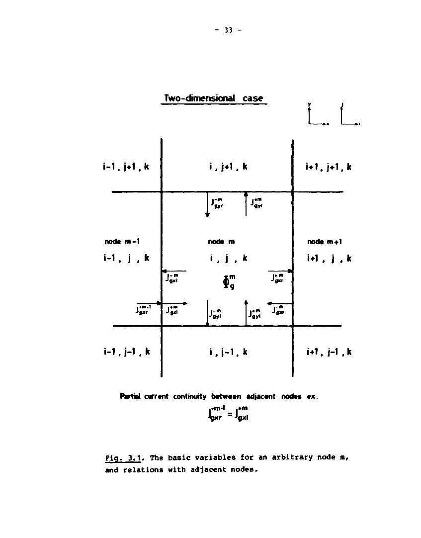
Two-dimensional case y i

i -1 . j * 1 , k i . j * 1 . k i * l . j*1.k

node m-1

i-1 , j , k

'fyr

node m

i , j . k

i - m 'gxl C

node m-fl

U1 , j . k

J* m 9"

. »m-1 ' i « r J *m ,-m

J awl • j r « l*m J Jgyt

«xr

i-1. H . k i , i - 1 . k i*1, j-1 , k

Partial current continuity between adjacent nodes ex.

i«nvl |»m Jgxr =Jgxl

Pig. 3,1. The basic variables for an arbitrary node m,

and relations with adjacent nodes.

- 34 -

The one-dimensional flux t* (u,t) can be expanded into a poly-rgu nonial

N u •;u(u) = t c»n.pn e-) (3.9) * n=0 * Au

In the basic variant of the nodal expansion Method • is expanded

to second order. The expansion functions that are used are

P0(u) = 1

Pl(u) = u

P2(u) = u2 - fj

(See moreover Appendix A.)

To satisfy the normalization condition

Au AU y *

and for the boundary conditions t?ur and ifqul the three coef

ficients are determined to

c?o - ••

^ 1 ' *Sur " »Sul (3-10)

cg2 ' 3<*gur + *gul " 2#g>

The diffusion theory gives an expression for the average surface

flux

•gus » 2<3g1!s * *g5s> (3-")

and the insertion of the expansion (3.9) into Pick's law (3.7)

results in a set of nodal equations which can be solved iterat-

ively.

- 35 -

By inserting Eqs. (3.11) and (3.10) into (3.9) the following

expression can be derived:

This expression for the one-dinensional flux in direction u can

now be inserted into Pick's law (3.7). First, the expression at

the left edge of a node (s*l, u = - -J- Au):

+ 6 ^ g u r • 3 g u r + 3 g ui + 3 g ui 9

q)l - 3 q ui 3 g u l

<=>

(3.12)

Correspondingly, at the right edge of a node (s=r, u *+ y Au):

^ l ^ J u r O g » r -(jjft * jgfc)]

• 6<^!r + 3gJr * jJSi • Ji5i - • ; ) } - jg»r - jgur

<*>

D * D * Dw D* D18

(3.13)

- 36 -

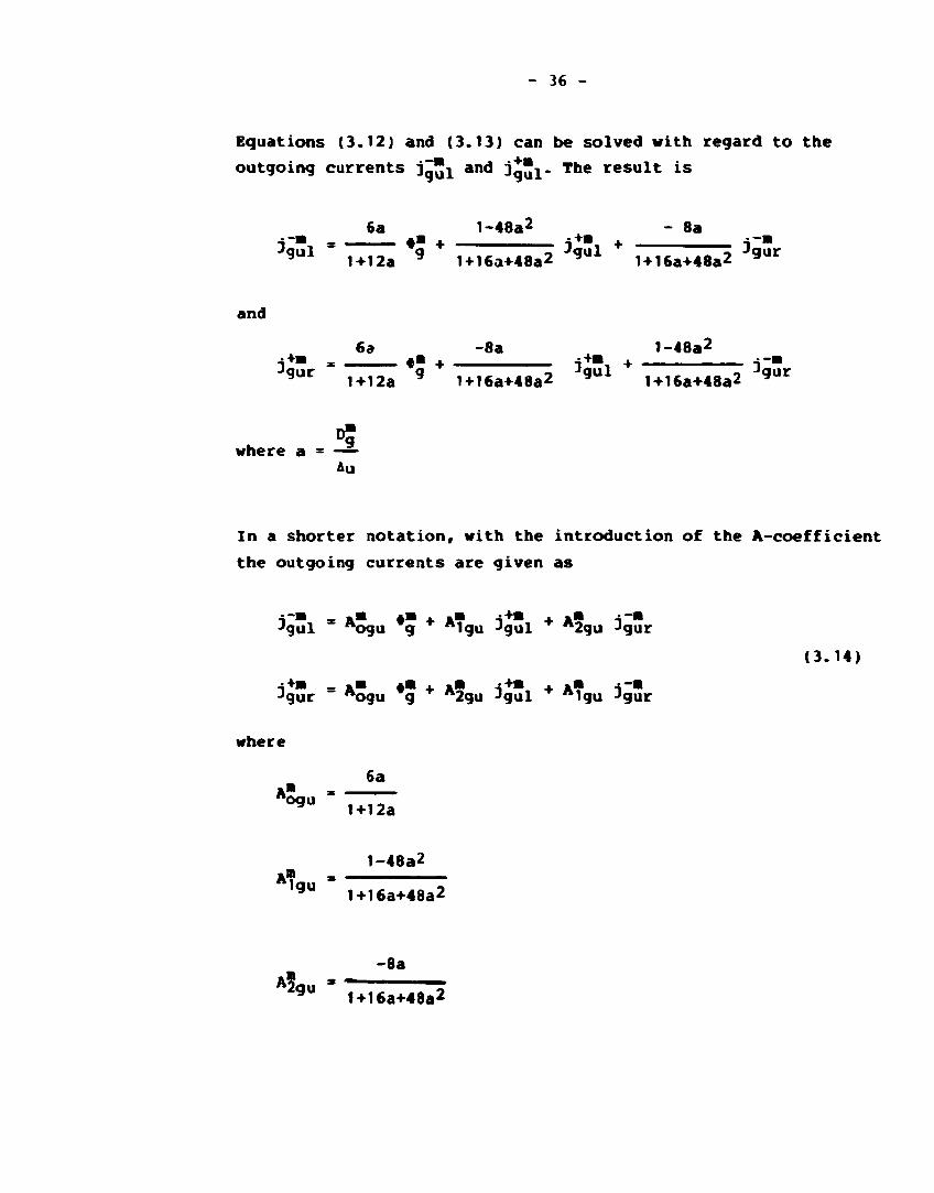
Equations (3.12) and (3.13) can be solved with regard to the

outgoing currents j " ^ and j-Ji- The result is

6a 1-48a2 - 8a

^ 5 l * TTT2T *" * 1+16a+48a2 j*!l * 1+16a+48a2 j« 5 r

and

6d -8a 1-48a2

j^"r = 7*̂ 1 *" + l+16a+48a2 j « ! l * 1+16a+48a2 j ^ r

D5 where a * —

In a shorter notation, with the introduction of the A-coefficient

the outgoing currents are given as

Jgul " "ogu g *1gu -»gul A2gu Jgur

Jgur Aogu g *2gu -»gul A1gu Jgur

where

(3.14)

A» 6a

ogu =

A1 9

1+12a

1-48a2

1gu 1+16a+48a2

-8a

2gu 1-H6a+48a2

- 37 -

The expression for the outgoing currents (3.14) can now be in

serted into the nodal equation, (3.5), to yield the final nodal

balance equation

7 ^ *5 = l 7 [2A3gu#g + <MVA5gu-1,(i9Si+igSr>] vg dt * u=xfy,z Au

+ E?g »g- 1 lZgV + (1-B)J~ vZfg']*S' + .l ̂ g ^ g =i A i=l

Rearranging

t - f. + l ^ N + Zrg]»5 » I [SgV-O-e) ^ v£?g- ]•?• vg dt u=x ,y ,z &" 9 y g '=l y y A y y

( 3 . 1 5 )

+ f / i4g c T + I 77 (1 " ATgu - A ? g u ) ( j g S l + 3g15r> 1=1 usx,y,z au

The A*s are g iven by

6a Am °9U 1+12a

1 - A? - Am S — — — = 4 • Am

' A1gu A2gu 1 + 1 2 a * Aogu

Now a iteration procedure can be outlined for the basic variant

of the nodal expansion method (NEM). Prom the preceding iter

ation step all average fluxes and outgoing currents are known.

The incoming currents can be found by the continuity condition,

Eq. (3.8). At the boundaries of the core the incoming currents

can be found by using some albedos.

In the general case an albedo-matrix is used with the possi

bility of down- (and up-) scattering in the reflector

- 38 -

jin = cfjout

Formally, the iteration procedure is:

1) Solve

1 d» = A * + B Jin + E • C

v dt in

dC = -AC + E *

dt

(3.16)

with regard to * and C for all nodes.

2) Calculate the outgoing currents

jout = G * + H • Jin (3.17)

3) Calculate new incoming currents with the continuity con

dition (3.8)

jin = p . jout

3.2. Stationary equations

The stationary equations are found by setting all time deriva

tives equal to zero and by neglecting the delayed neutrons.

Equation (3.15) now becomes

u*x,y,z A" g 9 g'-1 ** A 9 9

+l IS(1 " A V " ASgu)^gSl + ^Sr> u«x,y,z °u

- 39 -

The other equations, (3.14) and (3.8), are unchanged.

In the two-group theory the formal equations are

A • = B Jin (3.18)

jout = D • + E Jin (3.19)

where (3.18) are two equations with two unknowns per node which

easily can be solved and (3.19) are 12 equations. The continuity

equations can be written

jin = p jout

where P is some kind of permutation matrix.

3.3. Higher-order approximations

The basic variant of NBM with an expansion of Bq. (3.9) to second

order is unfortunately not very accurate and therefore the hie «r-

-order coefficients (third and fourth order) have to be deter

mined by additional calculations. The higher-order coefficients

can be determined by requiring that (3.9) solves the one-dimen

sional diffusion equation in a weighted residual sense. The one-

-dimensional equation in node m, energy group g, and coordinate

u, which are equivalent to Bq. 3.1 is

(3.20)

C* v T

- 40 -

where

•qU is the one-dimensional flux in node m, energy group

g and coordinate u.

Smu is the solution of the partially integrated precursor

equation

U mn 1 G

1 J 2 + VTu =7|i = /ivj:?a'*3'u (3.21,

LgU is the transverse leakage out of node m in the directions

v and w

j +1/2AV + l/2Aw a 3 3 3 Lm

u = ~ — / / [ Dm + Dm ]* (P,t)dvdw y u Au -1/2AV - 1/2AW

av y 3v 3w y 3w y

(3.22,

A^ approximation for the transverse leakage LqU can be obtained

by using leakage information from adjacent nodes, and a para

bolic representation has proven to be sufficiently accurate

Lgu " I LgVp<7-> <3-23> y n»o y Au

The coefficients are

- 41 -

L™ = L™ = — + ,out -out ^in ^in J v Jw ->v Jw

9° gu Av Aw Av Aw

.i-in +-;+ni ^-m +-;+n» Jgvl Jgvr Jgwl Jgwr

Av Aw

j+m +-;-ro .j+m .̂ — in Jgvl Jgvr Jgwl Jgwr

Av Aw

Tin _ T m _ i-in Lg1 " Lgur ^gul

*%2 - 3[(L5ur +L5 u l) - 2E5J

where L mu is the average transverse leakage for node m and di

rection u.

The boundary values L mu r and Lgul can be derived from continuity

conditions at the boundaries of each node

T ro-1 . fin Lgur Lgul

(3.24)

nffl"*1 T in-1 _ n't —. 1 "• Dg J^ Lgur * Dg j£ Lgul

where m-1 and m are numbers of adjacent nodes. Equations (3.24)

forms a tridiagonal system for the determination of the bound

ary values as functions of the average transverse leakages

Lgu*

To save calculations a linear approximation which fulfils Eq.

(3.24) is used.

- 42 -

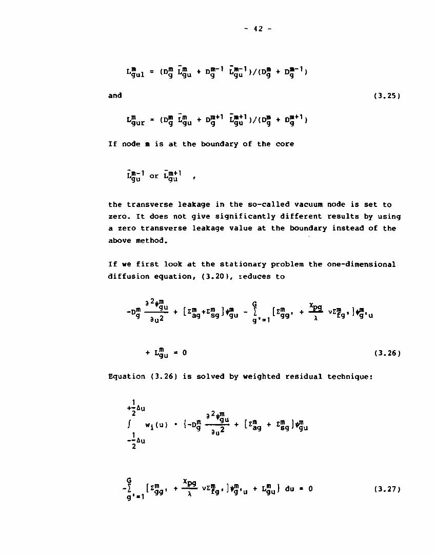
L5ul = l»q ^;u • D?"1 ^ - ^ / ( D j + D""1) gul *"g "gu g "gu

and (3.25)

L mu r = (D* L § U + D

m + 1 Lm;1)/(D5 + D m + 1)

If node m is at the boundary of the core

Lgu o r Lgu '

the transverse leakage in the so-called vacuum node is set to

zero. It does not give significantly different results by using

a zero transverse leakage value at the boundary instead of the

above method.

If we first look at the stationary problem the one-dimensional

diffusion equation, (3.20), reduces to

3 2^m G x

-D m 2iL + \zm +Zm l*n> - y fzm , + -22- vEm , l*"1,

+ L mu = 0 (3.26)

Equation (3.26) is solved by weighted residual technique:

1 +-Au

2 32^m

/ Wi(u) • {- i>g_|! i + [*5g + «Sg]#5u

- -Au

G . _ Xpg

~l,m [ z 5 g ' + \ vEV ]*g'u + L ? " } du * ° ( 3 - 2 7 >

- 43 -

The weight functions used in the weighted residual formula are

the same as the expansion functions for the one-dimensional flux

wj(u) = Pj(u) = u

w2(u) = P2( u ) = "2 " t?

The one-dimensional flux is expanded by (3.9) to N'th order and

the transverse leakage is given by (3.23).

With these terras inserted in the residual equation we obtain

1

2 N d2Pn(u) N f w-(u>'{-Dra ) cm + Zm • ) cm P (u) j Wjiui i "g i ^gnu , o rg L vgnufn,UJ

1 n=o du* n=o Au 2

G Xpq N

-) fEm , + -=-2- vE? • 1 • F c1™! P (u) g -1 A n=o

2 +1 L™Pn(u)}du - 0 (3.28) n=o

The only u-dependent variables in (3.28) are products of the

types

d2P.4(ll)

Pi(u)»Pj(u) and Pi(u) • -du2

and the integrals of these products are calculated in Appendix

A for various values of i and j.

With the weight function wj s Pj(u) and maximum order of four

(N=4) Eq. (3.28) gives the equation system

- 44 -

Dm

A,,2 2 *3u r* (12 °9lu 120 Cg3u> Au2

pg g.., W x fg° C

12 9 ,u 120 * 3u> + - Si

g = 1,2, ..., G.

The equation system is equivalent to

K11 * c?3u + K12 * c23u + ••• + K1G * cG3u = B1

K21 * c?3u + K22 ' c23u + --• + K2G " cG3u = B2 (3.29)

KG1 ' c13u + *G2 * c23u + •••• + KGG * cG3u = BC

where

11 2 Au2 120 rl 120 X1 \ fl

_L — Xpi

120 Kv ' —o CI'i + - r ^ i * J

»i - - H 'SicTiu • r2J.. /1?*' + ^T ^ » - * i u - 7; *

- 45 -

With the weight function W2 = P2(u) and maximum order of four

we obtain

->m 1 ,m _ _J „m

AU2 15 y'u ty 180 'g2u 2100

Dm a 1 1

- cg4u rg< «n cg2u 51ftn cg4u>

~ E <Z2a« + - T 2 v E f a ' H — cS'2u - — ' c2-4u) + — L m2 = 0

gt = 1 gg X f9 180 g 2u 2100 g 4u 180 g 2

g = 1 , 2 , ...» G

It gives the equation system

K11 * c?4u + K12 * c24u + ••• + K1G " cG4u = B1

K21 ' c?4u + K22 ' c24u + ••• + K2G * cG4u = B2 <3-3°>

KG1 * cT4u + KG2 * c24u + ••• + KGG * cG4u " BG

with

Kii s . L h L_ E« + JL.(if, + ̂ Ei vz5, 15 A u2 2100 tx 2

( Eft + - ^ vZ'f"i ) 100 xl X fl

1 Y *

JJ 2100 ^ X fJ J

1 1 § Xpi 1 i 180 ri i2u 180 ' * lg fg ' g'2u 18(J

ui2

- 46 -

The two equation systems (3.29) and (3.30) can easily be solved

with regard to the expansion coefficients by direct methods

(Gauss elimination). In the common case with only two energy

groups there are two equations with two unknowns that are to be

solved - but it is in every node in each direction!

The expansion function just found together with the lower-order

expansion coefficients from (3.10) can now be inserted in the

one-dimensional flux expansion (3.9)

*mu<u> . #m + 2 [ j * j r + .-^ _ ( j+ m i + J-J^J ±_

*UgSr + ^gSr + ig2l + 3gSl " W^* " ^

+ cS3u-P3^) + ^4u^4^)

The expansion is inserted in Pick's law (3.7) at the left edge

of the node (s = 1, u = - £ Au,

" l o\ -\ +"i 4.-4 ~m _/-i+m ± + -ro \ i — i2LDgur + D g u r " (Dgul + Dgul'-I &u

;+m x •;—m • j+ro b <3g u r + DgUr + lgul + 3gUl " *g>

2 g3u 5 cg4uJ ~ Jgul Jgul

<=>

D m Dm Dm n m n m <,+8 TJ^I • * •£ JSt • <1-8 && -4 i JS»+ 6 it *?

nm 9 1 m 1 m

- 47 -

Correspondingly, at the right edge of the node (s * r, u

+ ± A„)

D*

"T f^glr + 3i5r " CijSl + ig5l>l Au

l J gur Jgur Jgul Jgul g'

7 *-g3u c ^g4uJ ~ Jgur Jgur

<=>

D* D" D™ D m

4 i t J*~Sl + (,+8 && = -A~å jS5i + (1"8 -2»i5r

( 3 .32 )

D D

Equation (3 .31 ) and (3 .32 ) can now be so lved with regard to the

outgoing currents j g j j and j j j r

•i—ni _ »in AID + »m -s+in + »in -;~in Jgul ~ "ogu g "IguJgul rt2guJgur

+ A9 •r r o , - A1? •cjn* "3gu cg3u **4gu *-g4u

(3 .33)

Jgur "ogu g **2guJgul **1guJgur

A3gu*cg3u " A4gu*cg4u

- 48 -

With

5.. AU

the above A-coefficients are

6a

l+12a

1-48a2

1+16a+48a2

(3.34) -8a

1+16a+48a2

1 a

2 1+4a

5 1+12a 30 °9U

The expressions for the outgoing currents (3.33) are inserted

in the nodal equation, (3.5)

I T~ l2Aogu*g - 2A4gu • c™4u

u*x,y,z au

• <A?gu +A? g u-1,(jj; i • jj!r)]

G Xrvj

• E™ •«" « I (E«" + -SL vEfnf )•", 9 g g»»1 " x 9 g

Am "ogu

A?gu

A?gu

A? A3gu

A? ft4gu

- 49 -

Rearranging and using 1-*"gu-A2gu • 4Aogu

ll ^22H + !•>** = J (En + iBi vi" )•*. u=x,y,z Au rg 9 g' = 1 « x " 9

(3.35)

1 + u=x z * [4A5g«(Jg"l + j^r> + ^ ASgu ' cq*J

With higher-order expansion coefficients the steady-state iter

ation procedure is:

1. Calculate the higher-order expansion coefficients C3 and C4

from previous values of fluxes and currents.

2. Find the fluxes from A • • » B • Jln • B, • c4

3. Calculate new outgoing currents Jou^ =

D * • E Jin + B1 c3 + E 2 c4

4. Find the new incoming currents J*n = P • jout

3.4. Time-dependent theory

In the preceding paragraphs I have given a very detailed de

scription of the theory for the steady-state calculations with

the nodal expansion method. The theory for the time-dependent

problems is the same and the resulting equations are identical

with the exception of a few extra terms from the time-derivative

of the flux and from the delayed neutrons.

The expressions for the outgoing currents as function of incom

ing currents and average fluxes (3.33) are still valid for dy

namic problems. The nodal equation is obtained by combining

Bqs. (3.15) and (3.35)

- 50 -

v g dt u = x , y , z &" ' * g*=1 ** A ' *

(3 .36)

+ ? /i*ågci + I 77 £4A5gu<j<£l • 3g«!r) i=1 u=x,y,z

ic ogu cg4uJ

The time-derivative of the flux is approximated with a simple

first-order backward difference formula

d»J(t) t

- J j — I J I^Ct) -••(t-At)] (3.37,

which is inserted in (3.36). The term *g(t-At) is known from

the previous timestep.

The contribution from the delayed neutrons has to be calculated

by the precursor equation, (3.6). The solution of the precursor

equation is approximated by

Cf(t) * Cj(t-At) • e

-*iAt 1 Q 1-«

• [- I *i"*JQ**S,it) ] • (3.38)

The one-dimensional equation for determining the higher-order

coefficients (3.20) has two more terms than were included in the

derivation in Section 3.3. The first term is the derivative of

- 51 -

the one-dimensional average flux, and it is assumed that it has the same time-dependence as the node average flux. Moreover, it is also assumed that it has the same spatial dependence as the one-dimensional flux itself.

'•!u i i d*5

9 9 g

The time-derivative of the average flux is approximated by Eq. (3.37).

The second term which has to be added is the contribution from the delayed neutrons. The one-dimensional precursor ?q (3.21) has to be solved and it could also be done by weighted residual techniques. Instead of attempting this rather hard work, it is assumed that tbe spatial distribution of the delayed neutrons follows the flux distribution.

G I tg'u

C?u " * Cf (3.40) 6

g' = 1 *

and that it suffices to expand the local one-dimensional flux to second order.

With these additional terms the one-dimensional equation can be solved by weighted residual techniques in quite the same way as in the static case. The coefficients in Eq. (3.29) become

- 52 -

1 Di 1

AU2 120 ri 120 xl X flJ 120 vi

PI [q^c^^-v^] i*j

Xpj

12 ri llu 1 2 * . . i 1 9 * £g 9

L L- - L L !̂i . cm 12 i1 12 V i dt l1u

,ra 1 } 71*« J.,

1 cg'1u g'-l g

*k "Cf

g'-1 •J.

(3.30)

1 °i " T 5 — 2 - 2-100 Z?i + 2TO0 ^Ti * (''»I - f ^fil 15 A 2

1 1 f ^

2100 vi dt

- 53 -

K;, = — — [ZV. + (1-6) -£i vrm ] itj 13 2100 1D A £3

»i - - TiJ * • C?2u + TTO L , 1 ^ ' + (1"B) ¥ Vl?9']-;-2u

1 1 1 d*i

180 " 180 vi dt 1/u

G * cm. g'2u

1 I g =1

+ X d i l * • K ' Cm

180 dl k=1 G * E •*

g' = 1 g'

The general dynamic iteration scheme can now be outlined:

1. Calculate the higher-order expansion coefficients C3 and C4.

from previous values of fluxes, currents and delayed

neutrons.

2. Calculate the fluxes from

A'#(t) = B»Jin+B1 •c4+32,*(t-At)+B3'C.

3. Calculate new outgoing currents

jout s D*»(t)+E»Jin+E1 •c3+E2*c4.

4. Calculate new incoming currents jin s p.jout.

5. Calculate new values of the delayed neutrons

C(t) » P«C(t-At)+G*»(t).

- 54 -

4. PROGRAMMING

The nodal expansion method has been programmed in NEM, a program

divided in two parts, one for steady-state calculations and the

other for dynamic calculations. Before the dynamic part can be

run a steady-state calculation has to be made with a dump of all

variables to file as last output. Then the dynamic calculations

start with a restart from the dump file.

Each program consists of a main part and several subroutines as

shown on the structure diagrams in Figs. 4.1 and 4.2. In the

following the main parts of the program will be described in

more detail. The program structure is straightforward and it

should make it easy to combine with a hydraulic program.

Static version af NEM

»RI I

STMT WSTAH1 INCURR

3 ourp

OtTPU

om/r

— z SOIVS

AOt] FLUXIT OUTFUf (JUMP

HSVM]

Fig. 4.1. Structure diagram for the static part of the

NEM-code.

- 55 -

Dynamic version af NEM

OUMP Reran OVNIN so o POWER

our« jp

REFER

MAIN

MUUM FREC » F F

• -

INCURR MCOFF

/ / aoiMO TRMS

mTEOR

( M M

4

REJECT

\ 1 0

DOUM.E PMCO

* SOLVE

Fig. -1.2. Structure diagram for the dynamic part of the

NEM-code.

4.1. The steady-state main progr am

The main program consists all file declarations and all global

arraj declarations. The files used are described in the input

description in Appendix D.

The arrays, which have to be global are shown beneath. The array

dimensions should be equal to or greater than the values given

in the table. The letters used in the dimension sizes have the

following meaning:

G number of energy groups.

I number of nodes in the x-direction.

J number of nodes in the y-direction.

K number of nodes in the z-direction.

NAPP the approximation order + 1.

NNODE number of different fuel types.

- 56

Table 4.1

List of global arrays in the steady-state program

Name Dimensions Content

PI

CXL

CXR

CYL

CYR

CZL

CZR

CINXL

CINXR

CINYL

CINYR

CINZL

G,K,J,I

G,K,J,I

G,K,J,I

G,K,J,I

G,K,J,I

G,K,J,I

G,K,J,I

G,K,J,I

G,K,J,I

G,K,J,I

G,K,J,I

G,K,J,I

Average fluxes in each node and energy

group.

Average partial currents out of each

node in the x-direction at the left

edge.


node in the x-direction at the right

edge.


node in the y-direction at the left

edge.


node in the y-direction at the right

edge.


node in the z-direction at the left

edge.


node in the y-direction at the right

edge.

Average partial current., into each node

in the x-direction at the left edge.

Average partial currents into each node

in the x-direction at the right edge.


in the y-direction at the left edge.


in the y-direction at the right edge.


in the z-direction at the left edge.

- 57 -


CINZR G,K,J,1

P K,J,I

AX NAPP,G,K,J,I

AY NAPP,G,K,JrI

AZ NAPP,G,K,J,I

NODE K,J,I

D G,NNODE

SIGA G,NNODE

SIGG G,G,NNODE

USIG G,NNODE KHI

AA

BB

IPVT

IMIN

IMAX

JMIN

JMAX

G

G,G


in the z-direction at the right edge.

Average power in each node.

The A-coefficients in each node and

energy group in the x-direction.


energy group in the y-direction.


energy group in the z-direction.

Fuel type in each node.

The diffusion coefficients for each

fuel type.

The absorption cross sections for each

fuel type.

The scattering cross sections for each

fuel type.

The product of v and the fission cross

sections for each fuel type.

The emission spectrum.

Auxiliary array with the calculated

coefficients for the nodal equation

system.

Auxiliary array with the calculated

right side of the nodal equation system.

Auxiliary array with the pivot elements

for the nodal equation system.

The first node in the x-direction in

each row used in the geometrical de

scription of the reactor.

The last node in the x-direction in

each row.

The first node in the y-direction in

each column.

The last node in the y-direction in

each column.

- 58 -


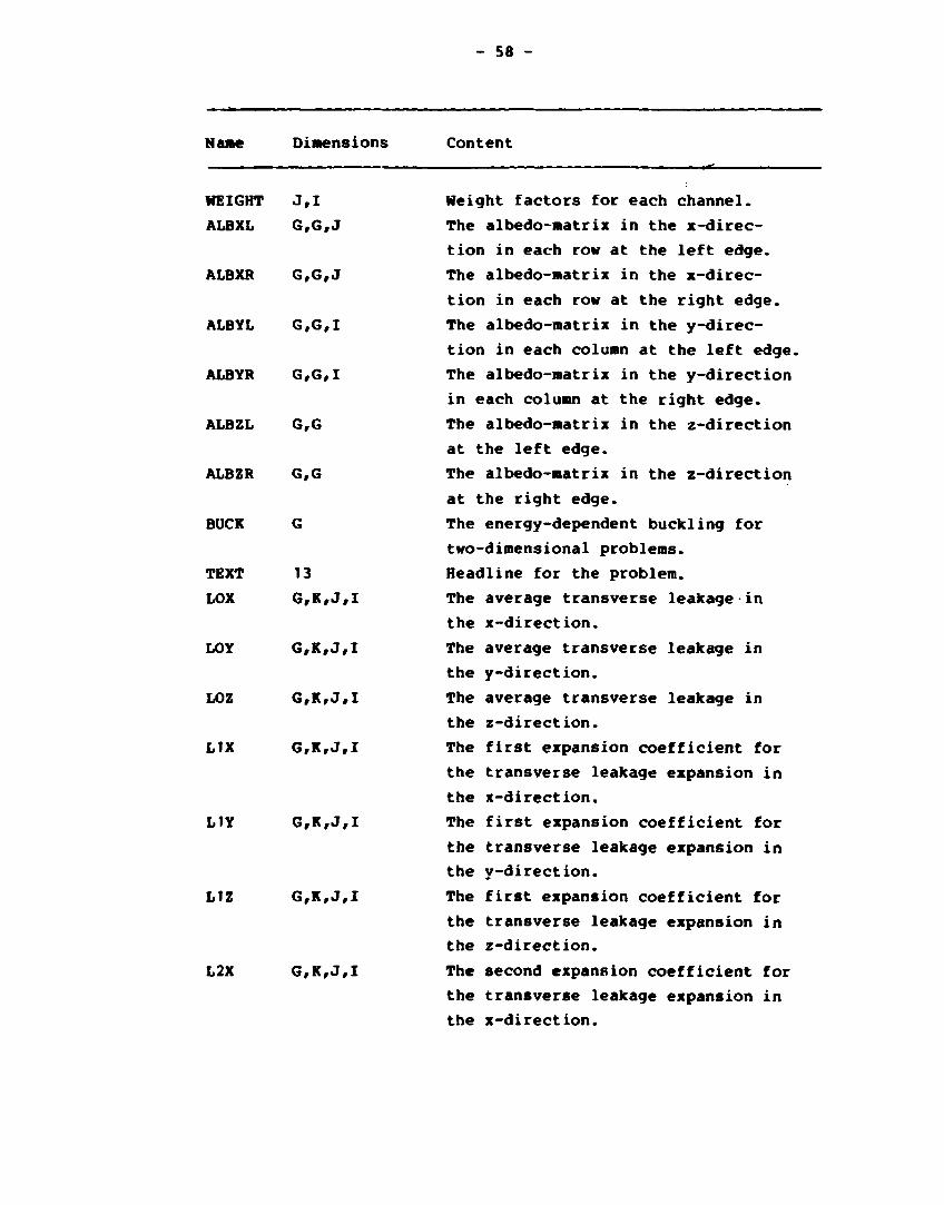
WEIGHT J,I

ALBXL G,G,J

ALBXR G,G,J

ALBYL G,G,I

ALBYR G,G,I

ALBZL G,G

ALBZR G,G

BUCK G

TEXT 13

LOX G,K,J,I

LOY

LOZ

LIX

L1Y

LIZ

L2X

G,K,J,I

G,K,J,I

G,K,J,I

G,K,J,I

G,K,J,I

G,K,J,I

Weight factors for each channel.

The albedo-matrix in the x-direc-

tion in each row at the left edge.

The albedo-matrix in the x-direc-

tion in each row at the right edge.

The albedo-matrix in the y-direc

tion in each column at the left edge.

The albedo-matrix in the y-direction

in each column at the right edge.

The albedo-matrix in the z-direction

at the left edge.

The albedo-matrix in the z-direction

at the right edge.

The energy-dependent buckling for

two-dimensional problems.

Headline for the problem.

The average transverse leakage-in

the x-direction.

The average transverse leakage in

the y-direction.

The average transverse leakage in

the z-direction.

The first expansion coefficient for

the transverse leakage expansion in

the x-direction.



the y-direction.



the z-direction.

The second expansion coefficient for


the x-direction.

- 59 -


L2Y G,K,J,I The second expansion coefficient for


the y-direction.

L2Z G,K,J,I The second expansion coefficient for


the z-direction.

The actual array dimensions (G,I,J,KrNAPP,NNODE) are read in

the main program. They are used for dynamic allocation of array

sizes in each subroutine, which also means that all arrays are

transferred through the head of each subroutine.

A route diagram for the main program is shown in Fig. 4.3.

4.2. Steady-state calculation

The steering routine for steady-state calculations is the sub

routine NEUTR. A flow-chart for the routine is shown in Pi^.

4.4.

The number of inner iterations for each outer iteration can be

chosen through the input. Besides the number of inner iterations

it is possible to choose an acceleration method. Prom Chapter

3.2 the stationary equations are

A«*(r) = e.jin(r-l)

jout(r) = D»*U) + E'Jin(r_1)

jin(r) = p.jout(r)

Where r is the inner iteration number. The iteration scheme for

the accelerated method is

- 60 -

Main program

V START J

define global array«

£ e a d 7 factual / / d i m e n s i o n «

steady state calculation NEUTR

no -•f STOP J

divide all nodes

PART

Piq. 4.3. Flow-chart for the main program for steady-

state calculations.

- 61 -

Steady-state (NEUTR)

V5TART J

read input initialize START

yn.

i calculate incoming current* INCURR

calculate A-coeffici ents A012

inner iterations FLUXIT

calculate incoming currents INCURR

calculate new eigenvalue

+f S T O P )

Pig. 4,4. Plow-chart for the subroutine NEUTR, which

contains the steady-state steering.

- 62 -

1. A«»(r) = BMin(r-l)

2. jout(r) s D»»(r) + EvjinU-1)

3.a.

lM r )

N F<r) = for MODE = 0,1

N

3.b. F ( r ) * max{«jr)} for MODE » 2,3 N

(4.1)

where *i is the average flux in energy group I in one node and

N is is the total number of nodes.

The mode to be used is selected by the input.

w 4.a. w(r> * 1 - Y [ U C O S ( • r)] for r odd

2 rtot

(4.2)

*

4.b. »*r* = 1 - Y{I+COS[ • (2'rtot + 1-r) ]} for r even 2 rtot

rtot is the total number of inner iterations, which has to be

fixed beforehand. Y is an input constant, and a value about 0.8

is optimum in most cases.

p(r)[A(r-l) + «{r-1)] 5. A(r) = (4.3)

F(r-1)[i + «(r-D]

1 6# jin(r) » . [P.jOut(r)+M(r).jin(r-1)l (4>4)

A(r)+u.(r)

This iteration scheme also normalizes the flux in each inner

iteration. The normalization can be done in two ways depending

on MODE, either on the average fluxes in group 1 or on the

- 63 -

maximum flux in group 1 (see step 3.a and 3.b). The best method

to use depends on the actual problem, but a normalization based

on the maximum flux (MODE = 2 or 3) is slightly faster than the

sum-method.

Unfortunately, there is only reliable convergence in the above-

described method for low local flux expansion order (second

order). Therefore, it is possible to make the iterations without

acceleration, but still with normalization. If NODE = 0 or 2 the

parameter « is set to zero in all iterations.

The total number of inner iterations per outer is given through

the input, but besides this a tolerance on the flux is given,

DF. In the inner iterations it is tested if

•«(r) - »(r-1)| < DF (4.5)

for all nodes and energy groups. If the above criterion is ful

filled in an inner iteration the maximum number of inner iter

ations for the next outer iteration is decreased to this number.

The calculation of the A-coefficients is not needed in every

iteration, if the cross sections and diffusion coefficients are

constant. With second-order local flux expansion they have to be

calculated only once and with higher-order expansions from the

viewpoint of minimizing the computer time an optimal procedure

would be to calculate them for every third inner iteration. If

the calculation of the A-coefficients becomes less frequent the

number of outer iterations drastically increases and the con

vergence is uncertain.

In the outer iterations the eigenvalue A is calculated. The

number of outer iterations is limited through the input, but the

iterations also stop when

I x(s) - x(s-1) | < d L ( 4 # 6 )

is fulfilled at the same time as the convergence criterion for

the fluxes is fulfilled, s is the outer iteration number. For

- 64 -

every five outer iterations, a new eigenvalue is calculated by

an Aitken extrapolation:

x(s-2) . x(s) _ x(s-l) . x(s-1) Xis) » (4_7)

X(s-2) + \(s) - 2 • A(s-l)

where x(s-2)r A(S-1) and x(s) a r e three successive calculated

eigenvalues. After an extrapolation of the eigenvalue is com

pleted a larger number of inner iterations are made to obtain

the full benefit of the better eigenvalue. The number is pro

portional to the third root of the total number of nodes and is

at least 20.

4.3. Steady-state input and initialization

All inputs except the array dimensions as described in Section

4.1 are read in the subroutine START, described in Appendix D.

Here some of the parameters will be described further. All input

variables are printed as soon as they are read.

It is possible to make a dump of all variables after a certain

amount of computer time. The time for dump, TDUMP has to be less

than the overall computer time limit, because the dump is made

after a full outer iteration. By restart nearly all variables

are read from dump-file and this is done in the subroutine

RESTAR.

The geometric shape of the physical problem can be widely

different. It is possible to take account of different symmetry

properties by the input variables ISYN and NSYH. The most common

types of symmetry properties and their influence on the input

variables are shown in Fig. 4.5. It is important to take sym

metry properties of a problem into account, because it greatly

reduces computer space and time.

The boundary conditions for a case is given by some albedo-

matrices and it is possible to have different albedo-matrices

- 65 -

GEOMETRICAL DESCRIPTION

FULL CORE:

NSYM=0

ISVM s 1

J = i • M 3 * « *

9 . 2 . 1 . 1 . 2 . 3 * . 5 . • . • » . *

KSVM = 3

l«7 J*7 • *J7«K

x 1 . 2 . 1 . 1 . 1 . 2 . 3 * 5 . « . 7 . » . » . • . *

HALF CORE: ISVM - 2 qnrtr

M * 1.1.1. 1.>.1 %X= I .J J.J 2.1

l«J

N * I 2 « K

JMM » I . J . J

r J«7 N*22»K

1.1.1.1.1.1.1 1 . J . * . * . * . 1 . 2

» 1 . 1 . 2 . 3 « 7 . 7 . « . $

QUARTER CORE: ISYM = *

l = J*3 t I

• t

R«I]«K

= 1 .1 .1 - 3.2.1

M I N stmm - i .1.1 . i M U > J N U > 4 . 4 . 3 . 2

EIGHTH CORE: ISYM =6

'*EP MM x 1 .1 .1 « t t l = 1.2.1

tvPfWH^H#7

1*2 i>3

MIN a 1,2

JMM 5 3.2

^

IMIN s 1 .1.1.1

WAX - 1.2.3.3

1*3 J««

JMIN = I .J .J

JMM * « . * . )

Pig. 4.5. Some of the most common possibilities for util

ization of symmetry properties for a certain problem.

- 66 -

in all boundary-channels (no z-dependence is possible). Most

problems are in two energy groups and some special cases are

described below

a n o12 Albedo-matrix = | | (4.8)

l21 °22

1. Fully reflecting boundaries: J*n s jout

a11 = a22 = *-0 (4.9)

°12 = °21 = 0.0

2. No incoming currents: Jin = 0

°11 = °12 = a21 * a22 ~ °.0 (4.10)

3. No flux at the boundaries: *D = 0

»II s «22 " - 1.0

(4.11)

°12 " °21 = 0.0

4. The boundary condition given by a gamma-matrix, i . e . as input to the TtfODlM-program (Lindstrøm N i e l s e n , 1971).

The gamma-matrix i s defined by

j = r • «

or

(;;)• ( 2 V N

- 67 -

Normally there is no upscattering in the reflector, so Y12 * 0»

With this assumption the albedo-matrix can be calculated by use

of the equations from the diffusion theory

1 - 2 • Y i i » I I "

1 + 2 • T11

a 1 2 = 0 ( 4 . 1 3 )

" • * *21 i 2 1 =

a 22 "

(1 + 2Tn )(1 + 2 *22>

1 - 2 • T22

1 + 2 • T22

For two-dimensional problems it is possible to give a buckling

instead of an albedo for the z-direction.

Besides the description of the problem some variables to be used

in the iterations are given by input (see the input description

in Appendix D). At last a number of options for the amount of

output have to be added. In one end it is possible to print

nearly all variables at every inner iteration (a huge amount of

output) and at the other end only the input is printed.

The flux-distribution is initialized to unity in the fast group

(Group 1). The other groups are initialized by

gin

•"= H?r * *™ (4*14) Eag

The outgoing currents are initialized to

jOut,m , j. . «m (4.15)

For 2 groups both are in agreement with the diffusion theory.

- 68 -

The array WEIGHT are initialized in accordance with the symmetry

properties for the problems. For nodes with cne symmetry line

through the node center WEIGHT = j and for nodes with two

symmetry lines through the center WEIGHT = j or -j fer $ -case.

4.4. The calculation of incoming currents

The incoming currents are calculated from outgoing currents in

the subroutine INCURR. For inner boundaries there are no prob

lems - the incoming currents are the outgoing currents ol ad

jacent nodes relaxed in accordance with Eq. 4.4. At the bound

aries of the case the incoming currents are calculated by use

of an albedo-matrix and the result is still relaxed a* de

scribed in Eq. 4.4.

In problems with symmetry, this symmetry is easily utilized by

the incoming and outgoing current notation. The incoming current

of a node at a symmetry line is simply the outgoing current of

its symmetrical counterpart.

For two-dimensional problems with a buckling, (El-Wakil 1962,

p. 109) the buckling is converted into an albedo-matrix in the

z-direction.

The basic z-dependent solution is

• (z) • C • cos(Bz • z)

The partial currents are obtained from diffusion theory

(Glasstone and Edlund, 1961, p. Ml)

• D d* JOUt a . —

4 2 dz

• D d* jin * — + — • —

4 2 dz

- 69 -

d* jin <t + 2 • D • —

dz Albedo » =

d* jout * - 2 • D •

dz

C cos(B*z) - 2*D*C,B*sin(B*z)

C cos(B»z) + 2*D»C«B»Sin(B«z)

1 - 2«B'D'tan(B»z)

1 + 2*B*D«tan(B*z)

The albedo has to be calculated at the node boundaries, so z *

-j- • DZ, where DZ is the node length in the z-direction, which

most suitably is set equal to the node length in the x-direc-

tion and/or y-direction.

4.5. Generation of A-coefficients

The calculation of the A-coefficients is done in the subroutine

A012. A route diagram of the routine is shown in Fig. 4.6.

The expansion coefficients for the transverse leakage approxima

tion (Eg. 3.23) are calculated in the subroutine TRANS by use of

Eq. (3.25). The transverse leakage at the boundaries is set- to

half the transverse leakage of the outermost node.

The higher-order A-coefficients A3 and A4 are calculated in a

special subroutine A34. An equation system of order G has to be

solved for each node and each coordinate. To solve the equation

system,

A • x * B

the square matrix A is L • U factorized by Gaussian elimination

with partial pivoting in the subroutine SOLVE. In the special

case with only two energy groups the solution is directlv cal

culated (the solution for two equations with two unknowns,.

- 70

Coefficients (A012)

y »

"approxi- % V t » rmtion order^,

>2

no

calculate Ap A, AJ

eq 3 32

calculate transverse leakages TRANS

U

calculate C s

eq 3 10

calculate higher order terms A34 eq 3 29-3 30

calculate At and A* eq 3 33-3 34

Pig. 4.6. Plow-chart for the subroutine A012, which cal

culates the A-coefficients.

- 71 -

4.6. Inner iterations

One inner iteration is made in the subroutine FLUXIT. For each

node the equation system (3.35) is arranged and solved by the

same routine as used in Section 4.5. Then the expression for the

outgoing currents are calculated and the convergence criterion

for the fluxes (4.5) is controlled. At last the A-constant (4.3)

is calculated.

4.7. Refinement

After a fully converged solution to a steady-state problem it is

possible to calculate a flux-distribution with finer nodes. The

number of nodes in each coordinate can be doublet, triplet,

etc.; the nodes are independent of one another. The generation of

new input data for the new nodes from the old ones are done in

the subroutine PART. The start distributions for fluxes, cur

rents etc. are the solutions from the coarser mesh calculation.

A special case is taken to treat symmetry properties, e.g. if

the old problem was a quarter case with symmetry lines in node

centers, the new case will have symmetry lines at node edges if

all nodes are halved in each direction.

The new total number of nodes still has to observe the absolute

limit for FORTRAN-arrays as described in Appendix D, so it could

be impossible to make refinements with full case problems. For

smaller problems, e.g. quarter cases, a refinement with a factor

two in all directions is possible, and it gives a good oppor

tunity to check the results. On the other hand, a factor two

in all directions provides about 8 times as many unknowns and

equations to be solved, which greatly increases the computer

consumption, so it is usually not practicable to continue cal

culations with finer nodes.

- 72 -

4.8. Dynamic main program

The dynamic main program for the nodal expansion method is also

the steering routine for the dynamic calculations. The dynamic

program is an extension of the steady-state program, so the ar

rays that are described in 4.1 are also used here. In addition

some other global arrays are declared, which mainly contain

fluxes and currents from preceding time-steps, and information

about delayed neutrons (see Table 4.2). The meaning of the

letters in Table 4.2 are

G number of energy groups

I number of nodes in the x-direction

J number of nodes in the y-direction

K number of nodes in the z-direction

L number of delayed neutron families

Table 4.2

List of special global arrays in the dynamic program


PIO

FI1

cxro

CXLI

CXRO

CXR1

G,K,J,I

G,K,J,I

G,K,J,I

G,K,J,I

G,K,J,I

G,K,J,I

Average fluxes in each node and

energy group one step back.

Averages fluxes two steps back.

Average partial currents out of

each node in the x-direction at

the left edge one step back.

Same, but two steps back.


each node in the x-direction at

the right edge one step back.


- 73 -

Mane Dimensions Content

CYLO GfR,J,I

CYL1 G,K,J,I

CYRO G,K,J,I

CYR1 G,K,J,I

CZLO G,K,J,I

CZL1

CZRO

C2R1

DPIDT

CO

BETA

DECAY

EXPDEC L

V G

G,K,J,I

G,K,J,I

G,K,J,I

G,K,J,I

L,K,J,I

L,K,J,I

L


each node in the y-direction at


Sane, but two steps back.


each node in the y-direction at




each node in the z-direction at


Sane, but two steps back.


each node in the z-direction at



The approximation to the time-

differentiated flux divided by

the average neutron velocity.

Average precursor distribution in

each node and family.

Same, but one step back.

The fraction of delayed neutrons in

each family.

The decay constants for the delayed

neutrons.

exp(-DECAY«DT).

The average neutron velocity for

each energy group.

Before a dynamic calculation can be performed a successful

steady-state calculation has to be made with a dump of the

final solution. The dynamic calculation then starts from the

- 74 -

steady-state solution with some additional input (see the

input description for dynamic calculations).

A route diagram for the dynamic main program is shown in Pig.

4.7. The calculations of cross sections and diffusion coef

ficients and their variation with time are made in the sub

routine PARAM. This subroutine must be made specially for each

problem. No streamlined input routine has been made because

various hydraulic feedbacks will have to be added when the

routine is built together with a hydraulic reactor model.

In the subroutine PREC the delayed neutron distribution is cal

culated from the preceding step. The initial precursor distribu

tion is assumed to be in equilibrium.

The calculation of the A-coefficients is made in the subroutine

DACOFF, which is much like A012 in the steady-state calcu

lations. It has to include only contributions from delayed neu

trons and from the time-differentiated flux. In dynamic calcu

lations the A-coefficients have to be re-calculated for each

inner iteration to guarantee convergence.

When the A-coefficients are calculated a new flux-solution and

new outgoing currents are calculated in the subroutine INTE6R.

The flux convergence is also checked in INTEGR, and there are

two different convergence criterions, which can be selected.

If MODE * 0 the convergence criterion is

y i •(r)/#(r-1) . j , i i n,g' n,g ' ' n,g

< DF (4.16) M • G

where the summation is over all nodes and groups.

- 75 -

f START J

re*4 ateaaW-• : « : • aalutian ftFSTAR

I raaa1 éWaamic input

I iaic talis«

SO

I calculate c r M i »rci

PARAM

I nak« precursor •tea

PIIEC

I calculate differential auatient

DIFF

I calculate incoming current«

INCURR

I calculal* A-cocffici«nt»

DAr.nrr

I find new HUB aoluiion

1NTEGR

1

®

•©

DOUBLE

•r*par« ^ r t c a r t . r f«r M m aevp

PRECO

Fig. 4.7. Plow-chart for the main program for dynamic calculations.

- 76 -

If NODE * 2 the convergence criterion is

I *(r) _ *(r-1) | < dP (4.17)

for all nodes and energy groups, r is the inner iteration

number. Criterion 4.16 is less stringent than 4.17 for the same

tolerancer DF.

The inner iterations are continued until the convergence cri

terion is fulfilled or the maximum number of inner iterations

is reached, as specified in the dynamic input.

If the fluxes have not converged after the maximum number of

inner iterations, the step is rejected and the step length is

halved. However, the step length cannot be halved indefinitely,

so a minimum step length can be specified in the input.

When it is possible to decrease the time step length, it also

must be possible to increase it again. The step length is

doubled when a number of satisfactory time steps have been

taken (the number is specified in the input) and when the

number of inner iterations per time step is less than one-third

of the maximum number. The last condition is given to prevent

cycling of the program between two step lengths with many re

jected steps as result.

After a successful step all variables are moved to get ready

for the next step.

Tc save inner iterations the fluxes and outgoing currents are

linearly extrapolated as a form of predictor step

At2 At2 • (t+At2) - d + )' *(t) - »(t-At,)

At 1 At j

where At] is the preceding step length and At 2 is the new step

length.

- 77 -

Por each time step the step length and the total power are

printed, but larger amounts of output e.g. power and/or flux

distributions can be printed with regular intervals. The

intervals are specified in the input.

5. EXAMPLES

In this chapter the results of the calculations with the NEM-

program will be reported. Some of the results are obtained

with special versions 01 che program to enable special effects

to be shown.

The program has been tested on various benchmarks which all are

described in Appendix B. Reference solutions and calculated

solutions are shown i;. Appendix C.

The solutions are usual!/ given with the eigenvalue (keff) and

the power distribution and their deviations from the reference

solution.

eigenvalue: X

eigenvalue error: AX = *~*ref nonwlly given in pern (10-5)

power distribution: P

maximum relative error:

Apmax » m a x pn ~ pref,n'

m pref,n

where n is all nodes. &Pjnax is normally given in per cent.

- 78 -

Average relative error:

1 N IPn " Pref.nl APav I N n = 1 pref,n

also given in per cent.

Two-norm of relative error:

/ £ pn " pref,n 0 AP2 = / I ( '—)2

"=1 Pref,n

Por three-dimensional benchmarks the power distribution is given

only for assemblies (average over vertical channels).

All CPU-times are on a Burroughs B7800 computer.

5.1. The IAEA-2D benchmark

The IAEA benchmark is one of the most famous (Nicheeisen, and

Neltrup, 1973). The two-dimensional benchmark is the midplane

of the three-dimensional one. The benchmark is described in

Appendix B.I and a reference solution in Appendix C.I. The

benchmark represents a reactor with a two-zone core and a water

reflector. Nine fully inserted control rods are represented as

smeared absorbers in a single node. Because of the control rods

and the water reflector severe flux tilts occur which make the

problem quite challenging.

A picture of the power distribution for one quarter of the core

is shown in Fig. 5.1. The figure gives a good impression of the

differences in the power level in the nodes. The flux de

pressions in the four noues with control rods are clear.

http://Pref.nl

- 79 -

Fig. 5.1. The power distri

bution for one quarter of

the core for the two-dimen

sional IAEA benchmark. The

distribution is normalized

to 1.J for the active part

of the core, which is the

part that has nodes with

power greater than zero

<Ff > 0).

The IAEA-2D benchmark has been solved with different orders and

different node sizes. A summary of the results are shown in

Table 5.1, where the first number in the order column is the

local flux expansion order and the second number is the trans

verse leakage expansion order. The transverse leakage expansion

order is at least two less than the local flux expansion order,

because there is no advantage, for example, in using second-

order transverse leakage expansion together with third-order

local flux expansion. The extra coefficient is simply unnecess

ary.

For each order the problem has been solved with different node-

sizes by use of the refinement feature in the program. When +24

outer iterations are stated in the table it means that additional

iterations are made and for the CPU (Computer Processing Units)

as well.

5.1.1. Orders and convergence

- 80 -

The errors in the eigenvalue as a function of the node size for

the various orders are drawn in Pig. 5.2, and in Fig. 5.3 the

Maximum relative error in the power distribution. The errors

here mean the differences from the reference solution (Appendix

C.I). There could be objections to making a comparison with a

solution that is obtained with another nodal program, but the

chosen reference solution is in good agreement with those ob

tained by quite different methods (e.g. finite-difference

methods).

Prom Pig. 5.2 and 5.3 it is seen in the first place that the

errors descend for smaller and smaller node sizes. In other words

the solution converges towards the correct solution, when the

node size moves toward zero. It is an essential characteristic

of a good method.

Secondly, the errors descend when higher-order expansions are

used. With coarse meshes we have to use fourth-order local flux

expansion and first- or second-order transverse leakage expansion

to obtain satisfactory results. Unfortunately, it is two to three

times more expensive to use fourth-order rather than second-order

expansions, because of the higher-order expansion coefficient

calculations. With second-order and constant cross sections we

need only to calculate the coefficients once.

In Appendix C.1 a typical solution together with the absolute

error is shown. The errors are largest in the nodes facing the

reflector. The error distribution is shown in Fig. 5.4.

- 81 -

Table 5.1. Solutions to the IAEA-2D benchmark for various orders

and node sizes.

11 inner iterations pr outer

2 inner iterations pr coefficient updating (except for second

order)

MODE = 2

Tolerance on eigenvalue: DL = 10~6

Tolerance on flux: DF = 10~*

Orders

2,0

3,0

3,1

4,0

4,1

4,2

Node size

cm

20.0

10.0

5.f

2.5

20.0

10.0

5.0

2.5

20.0

10.0

5.0

2.5

20.0

10.0

5.0

2.5

20.0

10.0

5.0

2.5

20.0

10.0

5.0

2.5

Outer iterations

32

+24

+39

+40

43

+ 15

+34

+35

47

+22

+15

+40

42

+9

+7

+34

47

+5

+ 19

+30

45

+5

+ 14

+29

X

1.02873

1.02901

1.02943

1.02966

1.02953

1.02974

1.02969

1.02966

1.02913

1.02959

1.02970

1.02966

1.02996

1.02973

1.02963

1.02960

1.02955

1.02968

1.02962

1.02961

1.02949

1.02966

1.02960

1.02959

AX

•105

-86

-58

-16

7

-6

15

10

7

-46

0

11

7

37

14

4

1

-4

9

3

2

-10

7

1

0

Apmax

%

22.9

16.9

7.7

3.5

13.0

4.6

1.7

0.97

13.3

3.4

1.7

1.1

2.6

1.2

0.56

0.20

1.6

0.97

0.46

0.31

1.3

0.77

0.29

0.13

AP2

%

55.8

42.9

20.8

11.1

29.8

12.3

5.2

3.2

32.3

9.9

5.9

3.6

5.6

2.5

1.1

0.34

4.1

2.8

1.6

1.0

2.8

1.6

0.75

0.39

CPU

sec

14.4

+26.4

+168.2

+684.6

27.5

+26.7

+182.3

+701.8

33.9

+50.6

99.5

+946.0

36.4

+ 19.9

+82.4

+941.7

44.5

+ 15.5

+59.3

+941.9

45.8

+ 16.7

+134.9

+979.0

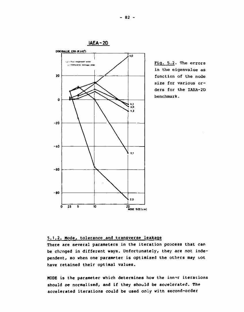
- 82 -

IAEA-2D

EIOENVALUE ERROR MO*)

20

-20

-«0

-60

-80

i.li - flux ••pantian order

j - trftntvrrrt. l . a k . f . o r *

•" 1 >vo

> * . i

» 3.0

3 * .2

> S.I

i 2.0

Fig. 5.2. The errors

in the eigenvalue as

function of the node

size for various or

ders for the IAEA-2D

benchmark.

0 25 5 10 20 NODE SIZE (cm)

5.1.2, Mode, tolerance^and transverse leakage

There are several parameters in the iteration process that can

be changed in different ways. Unfortunately, they are not inde

pendent, so when one parameter is optimized the others may not

have retained their optimal values.

MODE is the parameter which determines how the inn*r iterations

should oe normalized, and if they should be accelerated. The

accelerated iterations could be used only witn second-order

- 83 -

IAEA-2D

MAXIMUM RELATIVE ERROR IN POWER (V.)

Fig. 5.3. The maximum

relative error in the:

power distribution as

function of the node

size for various or

ders for the IAEA-2D

benchmark.

20 NODE SIZE(cm)

local flux expansions. With higher orders the iterations will

not converge. In Table 5.2 results with second-order local flux

expansion and different values of MODE are shown. The constant

y is 0.8, which is near the optimum value for this example. The

accelerated method is a little quicker, and it is also quicker

to use the maximum flux to normalize upon (NODE * 2 and 3) than

the average.

- 84 -

\ \ • i v

Fig. 5.4. The absolute er

ror distribution for one

quarter of the core for

the two-dimensional IAEA

benchmark.

^»o

With higher orders especially fourth order we have only to con

sider NOOB - 0 or MODE = 2. In Table 5.3 the IAEA-2D problem is

solved for different values of MODE. Strengthening the tolerance

requirement is also tried, but this has no effect on the accuracy

of the solution, and it takes longer time.

The column LEAK illustrates two different ways of treating the

transverse leakage expansion at the boundary of the core. LEAK =

1/2 means that the transverse leakage at the outer boundary of

the outermost node is set to half the average value. LEAK * 0

means that it is set to zero. There is no significant differ

ence and the standard is set to LEAK • 1/2.

Nor does it matter which MODE is used. However, MODE » 2 is

usually a little faster than MODE • 0.

5.1.3. Better start-values and inner iterations

In Paragraph 5.1.1 it was shown that it was necessary to use

fourth-order local flux expansion order and first- or second-

order transverse leakage order. Unfortunately, fourth-order ex-

- 85 -

Table 5.2. IABA-2D benchmark. 20-cm nodes second-order local

flux expansion order.

10 inner iterations per outer ones.

Tolerance on eigenvalue = 10~6.

Tolerance on power = 10" 4.

Mode

0

1

2

3

T

0

0 .8

0

0 .8

Outer I t e r a t i o n s

35

32

34

24

A

1.02875

1.02873

1.02872

1.02862

AX

*105

-84

-85

-87

-97

APmax

%

23.1

22.9

22 .9

22.3

AP2

%

5 6 . 2

55 .8

55 .5

52 .5

CPU

s e c

15.5

14 .4

15 .3

10 .4

Table 5.3. IAEA-2D benchmark. 20-cm nodes.

Fourth-order local flux expansion.

Second-order transverse leakage expansion.

10 inner iterations pr outer.

Mode

0

C

2

2

0

2

Ttelerance DL DP

10 - 6

10-7

10-6

10-7

10-6

10-6

10-4

10-5

10-4

10-5

10-4

10-4

Leak

1/2

1/2

1/2

1/2

0

0

Outer A i t e r ations

47

82

45

63

44

43

1.02951

1.02953

1.02949

1.02953

1.02950

1.02950

AX

•105

-8

-6

10

-6

-9

-9

APmax

%

1.35

1.52

1.30

1.33

1.50

1.60

AP2

%

3.0

3.4

2.8

3.3

3.5

3.3

CPU

sec

47.6

79.8

45.8

64.6

47.9

46.2

- 86 -

pansions are rather expensive* so here an attempt is made to

speed-up the calculations by using the second-order method in

the beginning to a certain point and then let the fourth-order

take over.

In Table 5.4 the results of such a strategy are shown, where

IT00T2 iterations are taken with 2,0 orders method and ITOUT4

iterations with 4,2 orders method. UPDATE is the number of

iterations between calculations of the A-coefficients, and it

has its optimum at 3. For longer intervals between calculations

the iterations would not converge.

The tolerance demand for the 2,0 orders method is lessoned by

some factors in proportion to the usual ones.

Tolerence on eigenvalue: DL2 = PDL2 * DL4

Tolerance on flux: DF2 = FDF2 * DF4

The optimum values are FDL2 = 100 and FDF2 = 12.

At last the number of inner iterations per outer ones can be

varied. The total computer time does not vary unambigiously with

the number, but there seems to be a minimum point around 20. The

optimum value for this example is 17.

These improvements have decreased the computer time by a factor

of three without losing accuracy. The optimum parameters found

m.iy not be optimum for other problems, but they can still manage

quite well.

- 87 -

Table 5.4. IAEA-2D benchmark. 20-cm nodes.

MODE = 3 (Y = 0.8) for second-order and MODE = 2 for fourth-order.

Inner Iteration

20

20

20

20

20

20

20

20

20

15

10

25

17

update

1

2

3

4

3

3

3

3

3

3

3 1

3

FDL2

100

100

100

100

10

1

100

100

100

100

100

100

100

FDF2

100

100

100

100

100

100

10

1

12

12

12

12

12

nOUT2

12

12

12

12

17

50

9

14

7

9

11

7

9

CPU2

4.1

4.0

4.1

4.0

5.0

11.9

5.7

10.7

5.1

5.0

5.3

5.7

5.2

ITOUT4

18

13

17

diverge

12

12

8

12

7

17

12

12

7

•105

-9

-11

-11

-8

-1

-4

-1

-9

-8

-8

-5

-8

APmax

1

1.31

1.35

1.36

1.42

2.28

1.78

2.27

1.25

1.42

1 33

1.74

1.20

CPU

sec

42.2

24.3

21.1

21.9

28.8

16.9

27.7

14.4

20.3

15.5

25.6

13.4

5.2. The IAEA-3D benchmark -r-

The IAEA-3D benchmark is described in Appendix B.2. The example

is much like the two-dimensional one but four partially inserted

control rods are also inserted. The benchmark has been cal

culated with 20 x 20 x 20 cm3 nodes and the results are col

lected in Table 5.5.

The results marked with a star are obtained with the procedure

described in Section 5.1.3 with the optimum iteration parameters

from the 2D-IAEA benchmark. The last solution together with the

absolute errors are shown in Appendix C.2. It is seen, that there

- 88 -

are no basic differences between the results for the two-dimen

sional benchmark and the results for the three-dimensional bench

mark, neither of which were expected. Still a saving of about

a factor 3 in computer time was obtained by using second order

in the first iterations.

Table 5.5. IABA-3D benchmark. 20-cm nodes.

MODE = 2

Tolerance on eigenvalue: DL = 10""*>

Tolerance on flux: DP - 1u~4

Orders

2,0

4,2

2,0*

4,2*

Outer iterations

44

62

12

+ 17

X

1.02797

1.02896

1.02685

1.02863

AX

•105

-106

-7

-218

»5

APmax

%

22.75

1.42

19.38

1.35

*Pav

%

8.45

0.77

5.41

0.66

CPU

sec

235

1235

115

+347

5.3. The Biblis 2D-benchma"k

The Biblis benchmark is described in Appendix B.3. The Biblis

benchmark is in two configurations, one without a control rod

and one with one in a node represented by a larger absorption

cross section in that node. Koreover, it is possible to rep

resent the reflector in three different ways: with an albedo

value, with one zone of reflector cross sections, and with two

zones. Illustrations of the power distribution-, are shown in

Figs. 5.5 and 5.6.

- 89 -

Fig. 5.5. The power distribution for one quarter of the

core for the two-dimensional Biblis benchmark. The

control rod is out (BIBLIS-1).

Fig. 5.6. The power distribution for one quarter of the

core for the two-dimensional Biblis benchmark. The con

trol rod is in (BIBLIS-2).

- 90 -

The calculated distributions are conpared with solutions obtained

with the finite-difference program TWODIM (Lindstrøm Jensen,

1971) and TVEDIM (Kristiansen, 1977). The reference solutions are

obtained with a mesh size of 2.89 cm. The solution for problems

1 and 3 and respectively 2 and 4 cannot be compared directly when

there is no assurance of good correspondence between reflector

cross sections and albedos.

Reference solutions:

Problem Program Keff

Biblis-1

Biblis-2

Biblis-3/1

Biblis-3/2

Biblis-4/1

Biblis-4/2

TVEDIM

TVEDIM

TWODIM

TVEDIM

TWODIM

TVEDIM

1.02398

1.01867

1.02520

1.02506

1.01970

1.01935

The benchmarks have been solved with orders 4,2 and with normal

tolerances (10~6 and 10"*) for different node sizes. The results

are given in Appendix C.3 and they are summarized in Table 5.6.

The results for the problems with reflector zones (3 and 4) are

in good agreement with those obtained with the finitedifference

code. If one or two reflector zones are used this has nearly no

effect. The two solutions are identical to within a few tenths

of one per cent. The deviations in Table 5.6 are merely caused

by the different reference solutions. The results are nearly as

good as they can be even with coarse meshes.

It is quite another case when the reflector is represented with

albedo matrices (1 and 2). Here there are deviations of about 10%

in the power distribution for large nodes, and the deviations

decrease to about 3% when each node is divided into 16 smaller

ones. This rather large effect of node size is quite unfortunate

considering the number of nodes, because it means that the use

- 91 -

of albedos for the reflector becomes rather difficult. Of course,

the reflector cross section representation can be used, but it

is, however, difficult to calculate these cross sections.

At last it has been tried to calculate albedos from the partial

currents at the boundary to the reflector in a calculation on

Biblis-3/2

iin a - g

9 " ^out Jg

The calculated albedos are shewn A.I Tab " 7 for different node

sizes, so the variation inside a large node can be seen. The

variation in the calculated albedos is largest *.i nodes at cor

ners of the core, where the deviation is about 20%, but if the

four albedos from the fine calculation are averaged they agree

with the coarse-mesh albedos to within a few per cent.

The calculated coarse-mesh albedos are used in the Biblis-1

benchmark and the results are compared with the Biblis-3/2 ref

erence solution. The results are shown under 1-A in Tab^e 5.6,

and the deviation from the reference solution is (of course)

small for large nodes, but it increases for smaller nodes.

The conclusion is that with the reflector represented by albedos

the results are rather sensitive to node sizes. A reflector re

presented with one (or more) reflector zones with cross sections

must be preferred, but it also means more nodes to the problem.

- 92 -

Table 5.6. The Biblis-2D benchmark. Fourth-order local flux

expansion. Second-order transverse leakage expansion. 17 inner

iteration per outer. MODE * 2. Tolerance on eigenvalue: DL =

10~6. Tolerance on flux: DF = 10~4.

Problem

1

2

3/1

3/2

4/1

4/2

1-A

Node size cm

23.12

11.56

5.78

23.12

11.56

5.78

23.12

11.56

5.78

23.12

11.56

5.78

23.12

11.56

5.78

23.12

11.56

5.78

23.12

11.56

5.78

X

1.02467

1.02424

1.02413

1.01921

1.01889

1.01881

1.02504

1.02511

1.02512

1.02505

1.02511

1.02513

1.01945

1.01948

1.01950

1.01944

1.01948

1.01950

1.02536

1.02494

1.02484

AX

•105

69

26

15

54

23

14

-16

-9

-8

-1

5

7

-25

-22

-20

9

13

14

30

-12

-22

ITOUT

22

+ 14

+7

28

+ 14

+6

23

+3

+7

27

+8

+8

27

+7

+6

26

-»-7

+6

21

+ 13

+7

^max

%

8.68

3.67

2.64

10.68

4.46

3.25

1.08

1.14

1.14

2.35

1.92

1.91

1.22

0.78

0.73

1.88

1.58

1.41

2.12

5.43

6.07

A*av

%

2.99

1.18

0.85

3.21

1.32

0.98

0.49

0.49

0.42

0.75

0.94

0.87

0.55

0.40

0.38

0.65

0.65

0.62

0.68

1.83

2.10

CPU

Sec

24

+41

+92

29

+41

+91

30

+ 14

+ 125

36

+33

+ 142

37

+29

+ 122

41

+33

+ 139

25

+42

+97

- 93 -

Table 5 . 7 . Calcu la ted albedos

with d i f f e r e n t mesh s i z e s .

Albedos in the y - d i r e c t i o n

I Group 23.12 cm 11.56 cm 1 2

1

2

1

2 ;

2

1

2

1

2

1

2

0.460

1.002

0.460

1.001

0.458

1.000

0.459

0.988

0.508

1.016

0.443

0.986

-

-

0.459

1.024

0.458

1.023

0.453

1.021

0.557

1.059

0.452

1.021

0.459

1.024

0.459

1.023

0.457

1.023

0.449

1.014

0.472

1.030

0.445

1.013

A.bedos in the x - d i r e c t i o n

J Group 23.12 cm 11.56 cm 1 2

7 1 0.537 0.580 0.499

2 1.025 1.067 1.038

8 1 0.584 0.634 0.515

2 1.044 1.088 1.045

i t h the B i b l i s - 3 / 2 benchmark

. - — , J «•! — •! - I I • • . ! • • II .

5.78 cm 1 2 3 4

-

-

0.459

1.029

0.458

1.029

0.455

1.027

0.6J4

1.0.0

0.455

1.027

-

-

0.459

1.029

0.458

1.028

0.452

1.026

0.513

1.053

0.449

1.024

0.459

1.029

0.459

1.029

0.457

1.028

0.449

1.024

0.479

1.038

0.445

1.022

0.459

1.029

0.459

1.029

0.456

1.028

0.451

1.010

0.464

1.031

0.448

1.009

5.78 cm 1 2 3 4

0.620 0.535 0.502 0.493

1.076 1.062 1.048 1.030

0.688 0.570 0.521 0.505

1.100 1.077 1.057 1.036

- 94 -

5.4 A typical Westinghouse PWR

The fourth example is an attempt to compare the calculated

assembly power distribution with measurements from a real reac

tor. To simulate a real reactor it is necessary to be able to

take feedback effects from the hydraulics in consideration. To

circumvent this difficulty the problem has been calculated with

the ANTI-code (Nielsen and Larsen, 1980) and finally, when the

code has converged, the cross sections and diffusion coef

ficients are printed for all nodes. The ANTI-solution is in

rather good agreement with the measurements and are also used

as reference (see Appendix C.4).

Thorlaksen, 1981 calculated an average gamma-matrix

0.1491 r = [

-0.0345 0.1624

and with an assumption on the proportion *2/*1, he found a

one-group albedo to 0.6. By use of the formulas in Chapter 4.3

an albedo-matrix can be calculated.

0.5406 0

" 0.8020 0.5097

If we use the same assumption on the flux proportion the albedo-

matrix can be diagonalized

Calculations with these parameters have been done, and the re

sults are shown in Appendix C.4 and summarized in Table 5.8.

With this example there is little benefit it> using second-order,

first and fourth-order later instead of using fourth-order

local flux expansion throughout the calculation.

Secondly, the deviations from the ANTI-solution are quite large,

and they decrease only slightly for smaller nodes. Surprisingly,

- 95 -

Table 5.8. Results for example 4 with use of the reflector

parameters calculated by Thorlaksen, (1981).

Albedo Orders Node Outer A A A A P m a x A p a v CPU size iter-cm3 ations %105 % % sec

a5 2,0 21.52*18.3 12 0.99300 300 9.7 4.2 77 'T

4,2 +31 0.99400 400 13.7 5.9 +563

4,2 21.52*18.3 38 0.99399 399 13.7 5.9 675

10.752x9.15 +14 0.99298 298 10.8 4.6 +1357

4,2 21.52*18.3 38 0.99443 443 15.7 6.8 661

10.752*9.15 +14 0.99346 346 12.9 5.3 +1372

the calculation with diagonal albedo matrices has the smallest

deviations.

The whole assembly power distribution is printed in Appendix

C.4 and it is compared with a calculation with QUANDRY (Smith,

1979) and with ANTI. There are very small deviations (less than

2%) between the NEM-solution and the QUANDRY-solution, but they

both differ quite much from the ANTI-solution. The NEM-solution

of the power distribution has too high power values near the re

flector and a depression in the center nodes, which could be due

to reflection properties in the reflector that are too good.

An attempt to produce better reflector parameters from the geo

metrical description of the reflector has been made. The reflec

tor is rather complex with corners and different materials as

shown in Fig. B.4. Two different reflector sets have been cal

culated, one in the axial direction and another average set for

the rest of the reflector.

At first the cross sections for the reflector are calculated

with the code CRSIQ (Lauridsen, 1977) and condensed to 2 groups.

It also calculates homogenised cross sections for the node size

- 96 -

used. The condensed cross sections are used in the program HBCS

(Pedersen, 1969) that calculates albedo- and gamma-matrices. The

reflector configuration used and the Cvsuits are shown in Table

5.9.

The new calculated reflector parameters are used in NEM and the

problems is solved for both albedo-matrices and reflector cross

sections. The resulting assembly distributions are given in

Appendix C.4. The two NEH-solutions agree quite well except in

some of the nodes facinc "he reflector, but the agreement with

the ANTI-solution has not been any better.

In Table 5.10 the average power for each layer in the core for

the four NEM calculations and with the ANTI solution as refer

ence. The boundary conditions in the z-direction are albedo-

matrices in all four calculations, also in the run with cross

sections as reflector representation. The albedo-matrices in the

z-direction are the same as used in x- and y-directions since

we have no better data. ANTI uses 0.6 in both top and bottom.

The 4 NEM-solutions do not differ very much from each other, but

they are flatter than the ANTI-solution, and in this direction

this is in better agreement with the measurements.

To make a final test of NEM a two-dimensional example has been

made by picking out the middle layer of the core. This problem

has then been solved by NEM and by TWODIM (Lindstrøm Jensen,

1971) and compared. Further on, a very fine modelling of the

reflector has been made with homogenizing of only each material

by itself (water, stainless steel) and with all details in the

core baffle and core barrel. It was also solved by TWODIM, but

with a very fine mesh (0.67 cm).

The results are shown in Table 5.11 for reflector cross sections

and in Table 5.12 for albedo- and gamma-matrices. With homo

geneous reflector cross sections the distributions agree within

0.5%, but not with the very fine calculation which is different

by about 15% near the reflector.

- 97 -

Table 5.9. New reflector calculations for example 4 with CRSIQ

and HBCS.

Average reflector

Axis reflector

Number of regions

Number of regions in fuel

Number of regions in core baffle

Number of regions in water

Number of regions in cere barrel

Radius of fuel

Radius of core baffle

Radius of water

Outer radius

24

5

3

14

2

10.0

12.5

27.5

31.5

cm

cm

cm

cm

24

5

3

5

10

10.0

12.5

17.9

31.5

cm

cm

cm

cm

Diffusion coefficient";,

group 1

group 2

Absorption cross sections,

group 1

group 2

1.32122 cm

0.291509 on

1.13855 cm

0.311097 cm

0.0015836 cm-1 0.0021617 cm"1

0.0348048 cm-1 0.050987 cm-1

Down scattering cross sections

1*2 0.027926 cm-1 0.0166602 cnT1

Albedo-matrix °11 a21

"22

0.589999

0.0426159

0.464227

0.611338

0.043182

0.465118

Gamma-matrix Tu

2̂1

Y22

1.28931

-0.0283048

0.182954

1.20602

-0.0182973

0.182539

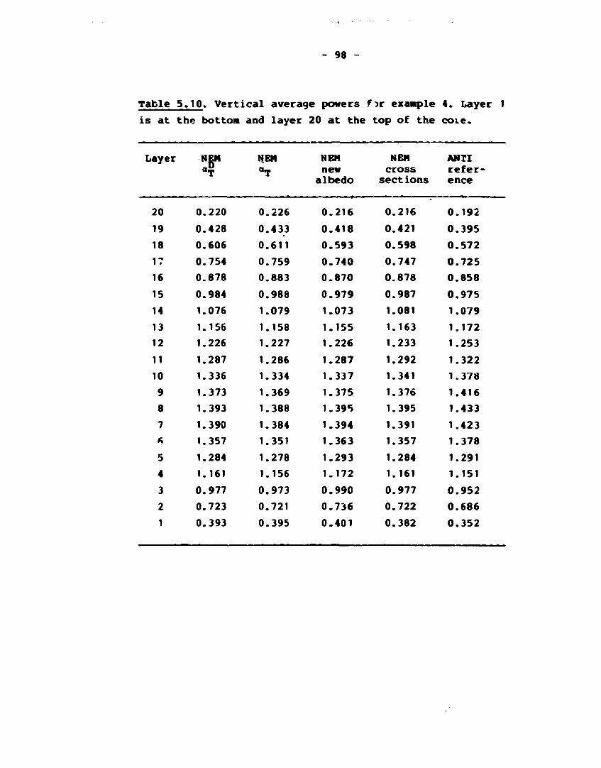
- 98 -

Table 5.10. Vertical average powers ftr example 4. Layer 1

is at the bottom and layer 20 at the top of the coie.

Layer NEM HEM NEM NBN AWT I df 0^ new cross re fer

al bedo sections ence

20

19

18

17

16

15

14

13

12

11

10

9

8

7

ft

5

4

3

2

1

0.220

0.428

0.606

0.754

0.878

0.984

1.076

1.156

1.226

1.287

1.336

1.373

1.393

1.390

1.357

1.284

1.161

0.977

0.723

0.393

0.226

0.433

0.611

0.759

0.883

0.988

1.079

1.158

1.227

1.286

1.334

1.369

1.388

1.384

1.351

1.278

1.156

0.973

0.721

0.395

0.216

0.418

0.593

0.740

0.870

0.979

1.073

1.155

1.226

1.287

1.337

1.375

1.395

1.394

1.363

1.293

1.172

0.990

0.736

0.401

0.216

0.421

0.598

0.747

0.878

0.987

1.081

1.163

1.233

1.292

1.341

1.376

1.395

1.391

1.357

1.284

1.161

0.977

0.722

0.382

0.192

0.395

0.572

0.725

0.858

0.975

1.079

1.172

1.253

1.322

1.378

1.416

1.433

1.423

1.378

1.291

1.151

0.952

0.686

0.352

- 99 -

Table 5.11. The power distribution for the central layer (10)

of example 4 calculated with reflector cross sections.

- -t..

0.950

0.951

0.956

1.098

0.928

0.927

0.927

1.062

1.021

1.021

1.025

1.152

1.009

1.005

1.004

1.103

1 .132

1 .127

1.131

1 .192

1.210

1.203

1.203

1.211

1.137

1.128

1.131

1.070

0.985

0.981

0.980

0.846

1.001

1.001

1 .006

1 .143

1.030

1.027

1.028

1.152

1.076

1.073

1.077

1.175

1.100

1.094

1.094

1.152

1 .142

1.136

1.140

1.139

1.101

1.097

1.095

1.022

0.781 0.787 0.785 0.637

1.070

1.068

1.073

1.183

1.06J

1.058

1.058

1.142

1.073

1.070

1.074

1.113

1.013

1.010

1.010

0 .993

1.011

1.020

1.019

0 . 8 8 8

1.054

1.051

1.054

1.109

0.976

0.974

0.974

0.985

0.957

0.961

0.960

0.906

0.706 0.722 0.718 0.585

NEN 21.5 cm nodes 0.895 0.757

NEM 5.375 cm nodes 0.894 0.774

TWODIM 1.34 cm 0.895 0.768

TWODIM, fine reference 0.67 cm 0.858 0.640

The eigenvalues are

HEM coarse mesh 0.99728 MEM fine mesh 0.99754

TWODIM 0.99758

TWODIM, reference 0.99468

- 100 -

Table 5.12. The power distribution for the central layer (2D)

of exanple 4 calculated with albedo- or ganna-natrices as

reflector representation.

0.991

1.039

1.062

1.098

0.967

1.010

1.026

1.062

1.060

1.103

1.121

1.152

1.040

1.071

1.076

1.103

1.156

1.178

1.182

1.192

1.225

1.227

1.220

1.211

1.146

1.122

1.114

1.070

1.001

0.957

0.946

0.846

1.041

1.088

1.108

1.143

1.067

1.106

1.118

1.152

1.106

1.139

1.150

1. 175

1.122

1.138

1.137

1.152

1.153

1.151

1.148

1.139

1.095

1.064

1.052

1.022

0.731

0.707

0 .699

0.637

1.103

1.140

1.153

1.183

1.087

1.110

1.114

1.142

1.087

1.096

1.099

1.113

1.017

1.003

0.997

0.993

0.959

0.932

0.926

0.888

1.069

1.079

1.084

1.109

0.978

0 .969

0.965

0.985

0.944

0 .910

0 .904

0.906

0.646

0.628

0 .623

0 .585

NEM 21.5 en nodes 0.881 0.666

NEM 5.375 en nodes 0 .840 0 .635

TWODIM 1.34 en 0.836 0.630

TtiODIM, l i n e reference 0 .67 en 0.858 0 .640

The eigenvalues are

KBM coarse nesh 0.99664

NEM fine nosh 0.99539

TWODIH 0.99550

TW0DIM, reference 0.99468

- 101 -

With albedo- and gamma-matrices the differences are not quite

as large, but in return results differ for different node sizes.

In Pig. 5.7 the two-group fluxes near and in the reflector are

drawn when they are respectively calculated with the reflector

homogenization code CRSIQ and with TWODIM with the fine reflector

modelling. The fluxes are normalized so the group 1 fluxes

coincide at the core boundary. The shape of the curves are the

same, but the levels in the reflector are not quite the same.

Figure 5.8 shows a picture of the fluxes in a cross section of

the whole core calculated with TWODIH. It is seen that the model

with the homogenized reflector is unable to predict the local

maximum in the thermal flux caused by the water in the reflec

tor. It seems a little thing, but it has a rather large effect

of the flux-levels in the middle of the core.

The attempt to compare calculations with real measurements

failed, but the code cannot be blamed. The problem is how to

treat the reflector and especially how to homogenize mixtures of

water and steel. The ANTI-solution agrees with the measurements

but AMTI also has several parameters, which can be fitted to the

problem.

- 102 -

FLUXES IN RADIAL DIRECTION.

1.6

12

0.8

0.4

00 -10

C » f *

X

\

•

— — CRSM3.group 1

—

V

— FINE TWOOtM. group 1

FINE TWrO0tM.group2

•**•«•». •'.• "••T>r*'*«,*-.'*"",*'*»«^ .: *•.*:•• v«N i ••—.̂ r—.*.«.

•

•

-

•

10 20 r/cm

Fig. 5.7. The two-group fluxes in the radial direction

around the boundary for the typical Westinghouse PWR.

The fluxes are calculated with, respectively, the TWODIM-

program and the CRSIQ-program.

FLUXES IN RADIAL DIRECTION.

1.0

0.8

0.6

0.4

0 2

0.0

• y r « M ^

Fine reflector model

Gamma matrix

»Homogenized reflector

^»*SwJsM

40 r/cm

Fig. 5.8. The two-group fluxes in the radial direction

for the typical Westinghouse PWR calculated with the

TWODIM-program with various reflector strategies.

- 103 -

5.5. Infinite slab reactor model

This very primitive benchmark is from The Benchmark Problem Book

(ANL, 1977) and the data for the example are given in Appendix

B.5. The example is calculated with 12 nodes each of 20 cm.

Whether the slab is in the x, y or z-direction does not matter,

since they are symmetric (for the use in this example).

The example is calculated with orders 4,2 and the dynamic sol

ution is given by the relative power fractions in each region.

The steady-state solution is

*eff Power

Power

Power

in region 1

in region 2

in region 3

NEM

0.90163

0.278

0.443

0.278

Reference

0.90155

0.279

0.442

0.279

The reference solution is obtained with a finite-difference code

WIGLB (Cadwell, Henry, Vigibotti, 1964) with 120 2-cm meshes,

and the solution is reported in The Benchmark Problem Book

(ANL, 1977).

Transient 1, a linear increment of 3% in the thermal absorption

cross section in region 1 in 1.0 second, is calculated with a

variable step length. The power distribution is printed in

Appendix C.5 and a diagram of the total power is shown ir Fig.

5.9. The total power decreases more than the reference »solution,

but it can be due to the slightly larger initial eigenvalue.

In transient 2 the thermal absorption cross section in .region 1

is linearly decreased by It in 1 second. The power distribution

(see Appendix c.5) is also lower than the reference solution in

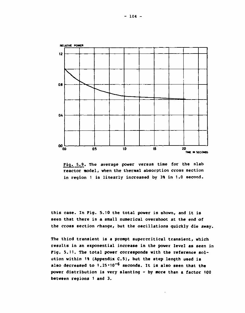
- 104 -

RELATIVE POWER

12

08

0.4

nn 00 0.5 1.0 15 20

TIME M SECON05

Fig. 5.9. The average power versus time for the slab

reactor model, when the thermal absorption cross section

in region 1 is linearly increased by 3% in 1.0 second.

this case. In Pig. 5.10 the total power is shown, and it is

seen that there is a small numerical overshoot at the end of

the cross section change, but the oscillations quickly die away.

The third transient is a prompt supercritical transient, which

results in an exponential increase in the power level as seen in

Pig. 5.11. The total power corresponds with the reference sol

ution within 1% (Appendix C.5), but the step length used is

also decreased to 1.25*10~* seconds. It is also seen that the

power distribution is very slanting - by more than a factor 100

between regions 1 and 3.

105 -

RELATIVE POWER

30

20

10

nn OJO

Fig .

1.0 20 30 40 TIME W SECONDS

5.10. The average power versus time for the slab


in region 1 is linearly decreased by 1% in 1.0 second.

RELATIVE POWER

101 r

104

10'

10'

10' r

10°

, -yC .J

: -T~ !

s -y — • ;

! -jT- ;

0.005 0.01 0.015 0.02 TIME M SECONDS


itsirt.r.r model, when the thermal absorption cross section

in region J u, »irtn.irly decreased by 5% in 0.01 second.

- 106 -

The last transient is the sane as the preceding one, but now

the average neutron velocities are 100 tines faster. It results

in a very fast transient and therefore it is followed only to

0.005 seconds. The step length quickly decreases to the smallest

allowed value and the program takes a lot of time steps without

fulfilling the convergence criterion; however, it does not seen

to affect the accuracy of the solution. The fast increase in the

power is shown in Pig. 5.12.

Table 5.13 shows the parameters which were used for the cal

culations. The computer times used are quite large, but it may

not be necessary to take so many time steps as were used here.

, RELATIVE POWER

ia*

10*

W

10'

10'

1 0 ° c

:

:

) t I 4 i 1 I i i

•

6 TME IN SECONDS ( « ' )



in region 1 is linearly decreased by 5% in 0,01 second.

The neutron velocities are 100 times larger than in

Fig. 5.11.

- 107 -

Table 5.13. Main parameters for the four transients in the

infinite slab reactor model.

Transient

2 3 4

Mode

Maximum number of

inner iterations

Minimum number of time

steps before step length

doubling

Tolerance on flux DP

Initial time step

Minimum allowed step

Minimum seep used

Maximum step used

CPU-time in seconds

20 20 20 20

5

10-5

10-5

10-6

10-5

0.0819

134

5

10-5

10-5

10-6

10-5

0.164

265

5

10-5

10~5

10"6

1.25*10-6

4*10-5

2620

5

10-5

10-5

1C-6

6.25-10-7

10-5

-2900

5.6. The TWIGL two-dimensional seed-blanket reactor kinetics

model

A description of the benchmark, which is found in Smith (1979),

is given in Appendix B.6. Two transients are initiated either by

decreasing the absorption cross section in region 1 by

0.0035 cm'1 either as a step perturbation or as a ramp pertur

bation in 0.2 seconds.

Steady-state solutions for this problem are obtained by fourth-

order local flux expansion order and various transverse leakage

orders. The results are shown in Table 5.14 and they are very

much alike. The steady-state power distribution is shown in

Appendix C.6 and a diagram of it is shown in Pig. 5.13. The

nodal size used is 8.0 cm.

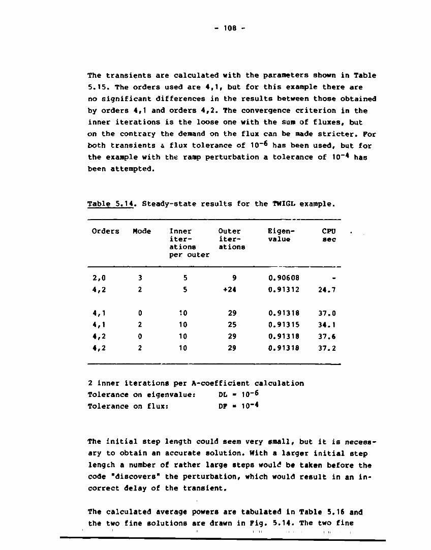
- 108 -

The transients are calculated with the parameters shown in Table

5.15. The orders used are 4,1, but for this example there are

no significant differences in the results between those obtained

by orders 4,1 and orders 4,2. The convergence criterion in the

inner iterations is the loose one with the sum of fluxes, but

on the contrary the demand on the flux can be made stricter. For

both transients & flux tolerance of 10~6 has been used, but for

the example with the ramp perturbation a tolerance of 10"* has

been attempted.

Table 5.14. Steady-state results for the TWIGL example.

Orders Mode Inner Outer Eigen- CPU iter- iter- value sec ations ations per outer

2.0 3 5 9 0.90608

4,2 2 5 +24 0.91312 24.7

4.1 0 10 29 0.91318 37.0

4.1 2 10 25 0.91315 34.1

4.2 0 10 29 0.91318 37.6

4,2 2 10 29 0.91318 37.2

2 inner iterations per A-coefficient calculation

Tolerance on eigenvalue: DL * 10~& Tolerance on flux: DP • 10~*

The initial step length could seem very small/ but it is necess

ary to obtain an accurate solution. With a larger initial step

lengch a number of rather large steps would be taken before the

code "discovers" the perturbation, which would result in an in'

correct delay of the transient.

The calculated average powers are tabulated in Table 5.16 and

the two fine solutions are drawn in Fig. 5.14. The two fine

- 109 -

Table 5.15. Main parameters for the two transients with the

two-dimensional TWIGL benchmark.

Perturbation

Ramp Step

Order Mode Maximum number of inner iterations Minimum number of time steps before step length doubling

Tolerance on flux Initial time step Minimum allowed step Minimum step used Maximum step used CPU-ti?»e in seconds

4,1 0 20

3 10-6 10-5 10-6

5»10-6 0.0410 2435

4,1 0 20

3 10-4 10-5 10-6 10-5

0.0819 269

5 0.

4,1 0 20

3 10-6 10-5 10-6 •10-6 .0819 2513

Table 5.16. Average power for the TWIGL-benchmark as function

of time.

Time

sec

0.00 0.05 0.10 0.15 0.20 0.25 0.30 0.35 0.40 0.45 0.50

Ramp-perturbation

Fine

MEM

1.000 1.131 1.316 1.577 1.972 2.082 2.090 2.098 2.105 2.113 2.122

Coarse

NEM

1.000 1.070 1.267 1.470 1.835 2.200 2.230 2.238 2.249 2.257 2.265

Quandry

1.000

1.307

1.957

2.074

2.092

2.109

Step-

NEM

1.000 2.065 2.081 2.088 2.096 2.104 2.111 2.117 2.124 2.132 2.141

-perturbation

Quandry

1.000

2.061

2.078

2.095

2.113

2.131

- 110 -

Fig. 5.13. The steady-state power distribution for one

quarter of the core for the two-dimensional TWIGL bench

mark.

TWIGL-2D BENCHMARK RELATIVE POWER

2.2

2.0

1.8

16

U

1.2

10

« /

* •

/ /

/ /

/ /

/ /

/

/ / / /

/ /

/ / r

f r

— t lamp par

(tap pa

iw paiion

rlurbattor t

00 01 0.2 03 0A 05 OB TIMC NSECONOS

Fig. 5.14. The average power versus time for the two-

dimensional TWIGL benchmark for respectively ramp- and

step-perturbation.

\

- Ill -

solutions are in good agreement with the QUANDRY-solutions, but

they also take lorg times to produce. The solution with the

coarse flux tolerance is nearly 10 times faster, but it is not

so accurate with about 8% deviation from the reference. The

normalized power distributions to various times are printed in

Appendix C.6 and though the average power increases with more

than a factor of two the largest changes in the po*er distri

bution are less than 5%.

5.7. The LMWLWR transient problem

This benchmark, which is a very simple model of a LffR was first

decribed by Langenbuch, Maurer and Werner (1977) and is there

fore called the LMWLWR problem. The benchmark is described in

Appendix B.7 and the static solution is shown in Appendix C.7.

The static solution is obtained with orders 4,2, and a nodal

size of 20 cm in all directions; it took 24 outer iterations

and 161 seconds of CPU-time.

The transient caused by some movements of the control rods is

calculated by two different methods. The method used in the pre

ceding, which yields very accurate but also very slow results,

is too slow for this three-dimensional calculation. The first

method (A) simply uses constant time steps independent of the

convergence of the fluxes in the inner iterations. In the prob

lems described in Paragraphs 5.5 and 5.6 a very small initial

step length was demanded, but this is circumvented by provoking

a lot of inner iterations (200) in the first step.

The method is tested with various step lengths from 0.1 second

to 2.0 seconds and the results are tabulated in Table 5.17. The

reference solution is obtained with QUANDRY (Smith, 1979), and

in Table 5.18 the deviations to the NEM-solutions are tabulated.

With time steps * 0.1 and 0.25 sec the solutions are quite good

within, respectively, 1% and 4%. A time step of 0.50 sec gives

an acceptable solution, but a rather large overshoot has oc

curred. Larger time steps give unacceptable solutions.

- 112 -

The second method uses variable time steps, but a much less

restrictive method for determining the step size is used. The

convergence criterion used in the step size determination is

moved from the inner to the outer iterations. The new conver

gence criterion for the outer iterations is based on the aver

age power in two subsequent time steps

|P(t) - P(t-At)| < DP

P(t)

The criterion is not really a convergence one, but it prevents

the solution from changing too much between each step. If the

criterion is unfulfilled, the step length is halved unless the

minimum step length is already used. The step length is doubled

when the relative power difference is less than half the power

tolerance and a number of time steps (specified in the input)

have been taken since last time-step change. The tolerance in the

power difference, OP must be set suitably and in this example

DP = 0.01 and 0.03 have been used.

The results are also tabulated in Tables 5.17 and 5.18, and they

are not quite as good as those obtained with method A. All the

solutions are graphically depicted in Fig. 5.15 and the solutions

obtained with method B have a rather peculiar behaviour. Both

solutions have some sharp peaks, which cannot be attributed to

any physical reason. This behaviour is caused by numerical over

shooting that would result in wild oscillations if the step

length were not drastically decreased. In the coarse case the

step length is decreased to 0.0125 seconds and in the fine case

it is decreased to 7.8*10~4 (minimum allowed) sec which would

bring the oscillations under control, but could not avoid the

peaks. Method A may be preferred for this example.

- 113 -

Table 5 . 1 7 . Parameters and r e s u l t s f o r t h e LMWLWR t r a n s i e n t

prob lem.

Program B B QUftNDKr

Orders 4,2 4,2 4,2 4,2 4,2 4,2 4,2 Mode 2 2 2 2 2 2 2 Maximum no of inner i t . 20 20 20 20 20 20 20

Initial step length 0.1 0.25 0.5 1.0 2.0 0.1 0.1 Minimum step length 0.001 0.001 •tolerance 10~2 10"2 10"2 10 -2 10"2 10~2 3'10 -2

P(0.0 s)

P(5.0 s)

P(10.0 s)

P(15.0 s)

P(20.0 s)

P(25.0 s)

P(30.0 SJ

P(35.0 s)

P(40.0 s)

P(45.0 s)

P(50.0 s)

P(55.0 s)

P(60.0 s)

pmax

T(Pmax) CPU

150.0

167.8

197.4

234.9

251.1

236.2

199.2

156.2

117.9

90.5

73.7

63.7

56.4

253.0

21.2

8062

150.0

163.7

197.7

232.2

253.8

244.2

203.8

156.0

117.4

89.7

71.5

64.0

56.1

255.9

21.75

3248

150.0

155.9

181.2

221.8

257.6

266.3

230.2

164.2

110.0

84.5

72.1

61.8

55.3

268.0

235

1705

150.0

154.4

161.7

179.6

205.9

230.9

236.5

216.9

178.0

114.0

53.1

15.0

12.2

237.9

29.0

889

150.0

158.7

169.4

183.0

181.3

138.2

71.6

186.3

34.0

460

150.0

167.8

198.1

234.4

255.3

262.0

299.0

166.7

126.1

95.8

77.0

66.7

59.0

262.0

25.0

7212

150.0

165.4

192.8

222.5

254.5

280.0

293.0

292.0

263.0

156.8

101.1

96.7

80.1

293.9

32.6

2583

150.0

167.1

196.9

250.3

201.0

119.0

74.1

56.9

V

- 114 -

Table 5.18. Deviations fro« the QOAMDRY reference solution in t

for the LMWLWR transient probles.

Method

Step length

Tolerance

T=5.0 s

T=10.0 s

T=20.0 s

T=30.0 s

T=40.0 s

T-50.0 s

T=60.0 s

A

0.1

0.4

0.3

0.3

-0.9

-0.9

-0.5

-0.9

A

0.25

-2.0

0.4

1.4

1.4

-1.3

-3.5

-1.4

A

0.50

-6.7

-8.0

2.9

14.5

-7.6

-2.7

-2.8

A

1.0

-7.6

-17.9

-17.7

17.7

49.6

-28.3

-78.3

A

2.0

-19.4

-32.3

-9.0

52.4

86.5

25.8

B

10-2

0.4

0.6

2.0

13.9

6.0

3.9

3.7

B

3-10-2

-1.0

-2.1

1.7

45.8

121.0

36.4

40.8

LMWLWR-30 BENCHMARK WeiATlVg POWElMW/cmM

0 K> 20 30 40 50 60 TMf M SeCONDS

Fig. 5.15. The average power density as function of

time for the three-dimensional UWIMR benchmark. Various steplengths and steplength selection strategies

are used.

*

- 115 -

5.8 The LRABWR two-dimensional benchmark

The LRABWR benchmark is a simplified model of a BWR in two

energy groups. The reactor has a two-zone core containing 312

fuel elements, each having a width of 15 cm. The core is re

flected by 30 cm of pure water and the control rods are rep

resented as smeared absorbers in four adjacent fuel assemblies.

The existence of the control rods causes severe local flu« per

turbations and the problem is rather difficult to solve. The

benchmark is completely described in Appendix B.8.

The steady-state solutions are shown in T*ble 5.19., where the

reference solutions are obtained by QUANDRY (Smith, 1979). The

results under 1 and 2 are for different orders and modes, while

result 3 is with orders 2,0 at the start and orders 4,2 at the

end. Result 4 is with finer nodes and the only difference be

tween 2 and 4a is the core geometry. It is seen that the com-

Table 5.19. Steady-state results for the LRABWR two-dimensional

benchmark.

1 2 3a 3b 4a 4b 4c 5

Rod position

Geometry

Node size in rm2

Orders

Inner it/outer

Mode

Outer iterations

Eigenvalue, X

AX-105

*Pmax *

APav * CPU seaonds

in V4 152

4,1 17

0

37 99626

-10 2.96

0.86

163

in V4 152

4,2

10 2

40 .99619

-17 3.89

1.13

154

in 1/8 152

2,0

17

3 7

.99598

-38 59.9

11.0

8

4,2

2

+26 .9961S

-17

4.13

1.26

+54

in

V8 152

4,2

10 2

44

.99619

-17

3.89

1.17

83

7.52

+14 .99630

-6 3.02

0.93

+76

3.752

+9 .99630 1.

-6 2.55

0.78

+211

out

1/4 152

4,1 17 2

40 .01508

-41 6.41

1.62

148

- 116 -

puter time is nearly proportional to the number of nodes. The

final results are for the situation with the control rod 12

withdrawn in the cold state. The normalized power distributions

are tabulated in Appendix C.8 and shown in Pigs. 5.16 and

5.17.

The transient of this benchmark is induced by the rapid with

drawal of a control rod. A very simple feedback mechanism is

built-in in this problem. The feedback model is specified by

two relations:

adiabatic heatup:

— T<r,t) * a'lEfjUftJ-^Uft) + Zf2<rrt}'*(r,t)J

and Doppler feedback:

Eal(r,t) = Zal(r",0)-[1+Y(/T<rrt) - /T^) ]

where a, Y and T 0 are known constants (see Appendix B.8 for a

complete description).

The problem has been solved by the three methods described above

and they are compared with a QUANDRY-solution. The average power

as function of time is tabulated in Table 5.20 and graphically

shown in Pig. 5.18. The average power increases by about 10

orders of magnitude, which is a very hard test for a computer

program for solving a numerical differential equation. The re

sults from the three different methods differ very much from

each other, but the shape of the curves in Pig. 5.18 are similar,

but time-displaced. The temperature is integrated by the backward

Euler method, which also introduces some errors.

The normal NEM method is stopped after about 1.7 second due to

exceeded process time. The method with constant time steps is

quite close to the normal method while method B has a time delay

of some tenths of a second which in its turn causes a higher

power peak. In Appendix C.8 the normalised power peak distribu

tion from method A is given at various times, and it is also

shown in pig. 5,. ^9.

- 117 -

Fig. 5.16. The power distribution for one quarter of

the core for the two-dimensional LRABHR benchmark with

the control rods in.

Fig. 5.17. The power distribution for one quarter of

the core for the two-dimensional LRABWR benchmark with

the control rods out in cold condition. (There is no

Doppler feddback).

\

118 -

Table 5.20. Kinetic results for the LRABWR two-dimensional

benchmark.

Program

Orders

Node

Maximum

no. of inner

Initial step

length

Minimum

step length

Tolerance

P(0.0 s)

P(0.4 s)

P(0.8 s)

P(1.2 s)

P(1.4 s)

P(1.6 s)

P(1.8 8)

P(2.0 s)

P(2.5 s)

P(3.0 s)

pmax,1

T(Pmaxrl) pmax,2

T(Pmax,2) used step:

Minimum

Maximum

CPU

seconds

it.

1.

2.

2.

6

NEM

4,1

2

20

0.002

10-4

0.01

10-6

36'10-6

53*10-6

89'10-5

12.2

165

-

-

-

-

6797

1.477

-

-

.25*10-5

0.032

80000

NEM, A

4,1

2

20

0.001

-

0.1

10-6

1.38*10-6

2.94*10-6

2.34*10"*

9.11

154

341

1093

139

74.1

7447

1.500

1098

2.006

-

-

26473

NEM, B

4,1

2

20

0.002

10-5

0.1

10-6

1.30*10-6

1.90*10-6

3.05*10*6

4.18*10-6

7.10*10-6

3.45*104

163

90.4

44.0

3.45*104

1.801

177.4

1.903

2.5*10-4

0.064

5721

QUANDRY

1.38

3.05

7.35

10-6

•10-6

•10-6

•10-4

720

79.8

97.4

5749

1.436

861

- 119 -

LRABWR-2D BENCHMARK

10*

10*

10*

10'

to'

,0°

10'

Iff'

10J

10*

10'

10*

RELATIVE POWER (W/cm>)

f "

! "

!

[

;

.

. t i

_r. ^r.r. **£

i

/ / /

"" /

i i i i t

i

i I •

. — • — • •

i i i .

UK. !

i i i i i i

r

V ^

— • — - MORHU. Ml

— — MTHOO i _ . - — . . MITMOO 1

' ^ 1 1 - »

]

i

—•-.C! J

ETHOO

I

j

i J

!

i

05 1.0 15 20 25 TIME M

30 SECONDS

Fig. 5.18. The average power versus time for the two-

dimensional LRABWR benchmark with a simple Doppler

feedback model. Various steplength strategies are used.

V

- 120 -

Time = 0.0 sec Time =0.8 sec

Time = 1.2 sec Time = 1.4 sec

Fig. 5.19a. The power distribution for one quarter of

the core for the two-dimensional LRABWR benchmark to

various times during the transient.

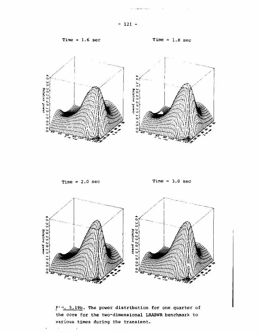
- 121 -

Time = 1.6 sec Time =1.8 sec

Time =2.0 sec Time =3.0 sec

F^. 5.19b. The power distribution for one quarter of

the core for the two-dimensional LRABWR benchmark to

various times during the transient.

- 122 -

5.9 The LRABWR three-dimensional benchmark

The preceding two-dimensional benchmark i s extended t o three dimensions with a core height of 300 cm and an ax ia l r e f l e c t o r of 30 cm water in each end. Only s t a t i c r e s u l t s are g iven here and they are summarized in Table 5 . 2 1 , where the r e s u l t s under 2 and 5 are obtained with the method described in Sect ion 5 . 1 . 3 . I t i s seen that there are great savings to be had by using low order in the beginning without los ing accuracy. The errors are ca lcu lated by comparison with a QUANDRY-solution.

Table 5 . 2 1 . Resul t s for the LRABWR three-dimensional benchmark.

Rod position

Geometry

Node size

in cm^

Orders

Inner it/

outer

Node

Outer it.

1

in

1/8

152*30

4,1

10

2 77

2a

in

1/8

152*30

2,0

17

3 11

2b

-

-

4,2

-

2

+20

3

in

1/4

152*30

4,1

17

0 42

4

out

1/4

152*30

4,1

17

0

43

»

5a

out

1/4

152*30

2,0

17

3 12

5b

-

-

-

4,2

-

2 +34

Eigenvalue X .99617 .99600 .99617 .99628 1.01512 1.01303 1.01500 AX',05 -22 -39 -22 -8 -37 -246 -49 Apmax * 1-95 24.43 3.42 2.11 2.45 75.91 3.63 APav % 0.61 - - 0.64 0.67 16.43 0.99 CPU sec 1690 128 +454 2123 2155 253 +1033

- 123 -

6. CONCLUSION

In the preceding chapters I have described the development of a

program based on the Nodal Expansion Method. The program is div

ided into two main parts: one for the steady-state calculations

and another for the dynamic calculations. The subroutines used

in the two parts are very much alike, so the steady-state routine

is described most intensively.

The program has been tested on a number of examples with good re

sults. The calculations can be made with various approximations

and acceleration methods. The results for calculations with high

orders (fourth-order local flux expansion order and first- or

second-order transverse leakage expansion) are very accurate when

compared with other calculations (finite difference, etc.). The

calculations are also rather fast compared with other programs

for the same accuracy. The nodal code ANTI is faster, but it also

uses only a 1 1/2-group method, while NEM uses 2 groups or more.

It has also been tried to make calculations on a real reactor

and then compare the results with measurements. This attempt

was more unsuccessful - the calculated power distribution dis

agrees significantly from the measurements. The cause of this

discrepancy was investigated, and the main indefiniteness lies

around the boundary conditions at the reflector.

The reflector can be represented in two ways, either by some

albedo-matrices or by cross sections and diffusion coefficients

with an outer boundary condition of zero flux or zero incoming

currents. The albedo-matrix representation is the most favourable

with respect to the number of variables; however, the solution is

changed for different node sizes with the same albedos. With the

reflector represented as a reflector zone of additional nodes the

solutions are nearly independent of node size, but the number of

nodes increases a lot; besides it is a problem to calculate homo

genized and condensed material constants for the reflector. Sev-

- 124 -

eral attempts have been made to mak? a good reflector representa

tion, but with no great success. The reflector representation or

perhaps the whole homogenization procedure has to be researched

further.

The program has also been tested on dynamic problems, but with

not such great success relative to the steady-state calculations.

The time steps that are to be used for accurate calculations are

very small slowing down the code. Several time step selection

strategies have been tried, and some of them work rather well,

but depend on the problem to be solved.

The program uses a direct method to solve the time-dependent

problems, which means that the time-integration and the space-

solutions are fully integrated, but perhaps it is necessary and

also satisfatory to use a quasi-static method. Purther inves

tigations must show this, and besides a hydraulic model has to

be built in, which may move the problems to other places in

the assembled program. The hydraulic part can be taken from the

ANTI-program, and in ANTI the hard points are in this part.

The examples I have used are mostly commonly known benchmarks and

the reference solutions are calculated with other codes. Someone

could claim that it is very well to compare the results with the

results obtained with other codes, but if they all are wrong,

they may have little to do with the real world. The statement is

partly true. If the program describes the whole reactor with

hydraulic feedback, pumps, turbines, etc. it is true, but if a

single part of this program complex is taken out, it is nearly

impossible to compare the results from this part with measure

ments. The program part has to be set in the right surroundings

and often these surroundings disturb the results completely,

which also are seen by the example with the typical PWR. m that

example, the hydraulic part was coupled off, the homogenizat.lon

was done, etc., but nevertheless a problem with the neutronic

boundary conditions disturbs the solution. Therefore the only way

to verify a program often is to compare with the results from

other codes.

- 125 -

As a final remark, some remaining problems, improvements and pos

sibilities for the Nodal Expansion Method and the NEM-program at

Risø National Laboratory will be outlined.

1. Introduction of hydraulic, either NEM in ANTI or reversed.

2. Improvement of the time step selection algorithm.

3. Investigations for a better reflector representation.

4. Introduction of Koebke's discontinuity factors.

5. Introduction of a possiblity for node interior cross section

variation, especially around control rods.

REFERENCES

Argonne Code Center (1977). Benchmark Problem Book. Numerical

Determination of the Space, Time, Angle, or Energy

Distribution of Particles in an Assembly. Argonne National

Laboratory - 7416.

BABALA, D., BECH, N., HAUGSET, H. (1971). ANDYCAP - Vol. 1 -

Theory SRD440.

BØRRESEN, S. (1981). Experience, Status and Advanced Applica

tions of PRESTO. Proceedings of the International Topical

Meeting on Advances in Mathematical Methods for the Solu

tion of Nuclear Engineering Problems. Miinchen, 27-29.

April 1981, p. 283-297.

CADWELL, W.R. HENRY, A.P., and VIGILOTTI, A.J. (1964). WIGLE -

A Program for the Solution of the Two-group Space-time

Diffusion Equation in Slab Geometry. Westinghouse Electric

Corporation, Bettis, Atomic Power Laboratory Report WAPD-

TM-416.

CADWELL, W.R. (1967). PDQ-7. Reference Manual. WAPD-TM-678,

Bettis Atomic Power Laboratory.

DORNING, J. (1979). Modern Coarse-mesh Methods - A Development

of the '70's. Proceedings of an ANS Meeting: Computational

Methods in Nuclear Engineering. Williamsburg, Virginia,

April 23-25, 1979, p. 3.1-3.31.

- 126 -

EL-WAKIL, N.N. (1962). Nuclear Power Engineering. (McGraw-Hill

Book Company, New York). 556 pages.

FINNEMANN, H. (1975). A consistent Nodal Method for the Analysis

of Space-Time Effects in large LWR's. In:

Proceedings of the Joint NEACRP/CSNI Specialists' Meeting

on New Developments in Three-Dimensional Neutron Kinetics

and Review of Kinetics Benchmark Calculations, Garching

(Munich) January 22-24, 1975, 133-170.

FINNEMANN, H., BENNEWITZ, P. and WAGNER, M.R. (1977).

Interface current techniques for multidimensional reactor

calculations. Atomkernenergie 30, 123-128.

FRANKE, H.P. (1977). Anwendung der Methode der finiten Elemente

bei der Berechnung drei-dimensionaler reaktor-

physikalischer Probleme. Atomkernenergie 3MD. p. 88-94.

GLASSTONE, S. und EDLUND, M.C. (1961). Kernreaktortheorie.

Springer-Verlag, Wien, Deutschen Ausgabe. 341 pages.

JAGANNATHAN, V. (1983). Evaluation of the finite-element-

synthesis model using the 3-D finite-element technique.

Annals of nuclear energy 2£ pp. 569-578.

KOEBKE, K. (1978). A New Approach to Homogenization and Group

Condensation. In: Homogenization Methods in Reactor

Physics, held in Lugano, 13-15 November 1978 (IAEA-TECDOC-

231) p. 303-323.

KRISTIANSEN, G.K. (1976). The finite-difference neutron

diffusion programme TWODIM. Risø-M-1891.

KRISTIANSEN, G.K. (1977). The two-dimensional finite-difference

programme TVEDIM. Risø-M-1919.

LANGENBUCH, S., MAURER, W. and WERNER, W. (1977a). Coarse-mesh

Flux-expansion Method for the Analysis of Space-Time

Effects in Large Light Water Reactor Cores. Nuclear Science

and Engineering 6_3 p. 437-456.

LANGENBUCH, S., MAURER, W. and WERNER, W. (1977b). High-order

Schemes for Neutron Kinetics Calculations, Based on a Local

Polynomical Approximation. Nuclear Science and Engineering

64, p. 508-516.

LARSEN, A.M.H. (1973). CRS: A Code to produce Multigroup Neutron

Cross Sections for Reactor Physics Calculations. Risø-M-

1568.

- 127 -

LARSEN, A.M.H. (1980). The Three-Dimensional PWR Transient Code

ANTI; Rod Ejection Test Calculation, Risø-M-2209.

LARSEN, A.M.H. ('983). Personal communication.

LARSEN H. (1971). SYNTRON, A Three-dimensional Flux Synthesis

Programme. Risø-M-1346.

LAURIDSEN, B. (1977). CRSIQ: A Cluster Programme to produce

Multigroup Cross Sections. RP-12-77. 17 pp. Risø National

Laboratory.

LAWRENCE, R.D. (1979). A Nodal Green's Function Method for

Multidimensional Neutron Diffusion Calculations.

Dissertation (Ph.D.), University of Illinois, Urbana II.

LIEBEROTH, J. (1977). An approximation of finite-difference

methods for diffusion problems by a coarse-mesh method.

Atomkernenergie 3_0, p. 103-106.

LINDSTRØM JENSEN, K.E. (1971). Development and Verification of

Nuclear Calculation Methods for Light Water Reactors. Risø

Report No. 235. 161 p.

MICHEELSEN, B. and NELTRUP, H. (1973). The 3D-IAEA Benchmark

Problem. Risø-M-1572.

MISPELDT, I. (1975). Solution of the Multigroup Neutron

Diffusion Equation by the Finite Element Method Risø-M-

1809.

NAKATA, H. and MARTIN, W.R. (1983). The finite element response

matrix method. Nuclear Science and Engineering 8j>, 289-305.

NIELSEN, E.F. and LARSEN, A.M.H. (1980). Input Description for

the Three-dimensional PWR Transient Code ANTI. Risø-M-2256.

PEDERSEN, J. (1969). Calculation of Heterogeneous Constants for

Cylinders and Slabs. Risø-M-850.

RYDIN, R.A. and SULLIVAN T.M. (1978). A new approach to the

QUABOX-CUBBOX coarse-mesh methods. Advances in Reactor

Physics.

SCHOUGAARD, B.F. (1979). A short Description of the Programme

NOTAM. Risø RP-19-79.

SIEWERS, H. and JAGER, W. (1977). Comparison of coarse-mesh

methods for benchmark and realistic reactor problems.

Atomkernenergie 30 p. 107-112.

- 128 -

SMITH, K.S. (1979). An analytical nodal method for solving the

two-group, multidimensional, static and transient neutron

diffusion equation. Masters thesis, Massachusetts Institute

of Technology.

THORLAKSEN, B. (1981). Construction of PWR Nuclear Cross

Sections for Transient Calculations. Test of ANTI Program

Against TWODIM. Risø-M-2264.

VONDY. D.R., FOWLER, T.B. and CUNNINGHAM, G.W. (1977). VENTURE:

A Code Block for Solving Multigroup Neutronic Problems

Applying the Finite-Difference Diffusion-Theory

Approximation to Neutron Transport, Version 2. ORNL-5062/R1.

WACHSPRESS, E.L., BURGESS, R.D. and BARON, S. (1962).

Multichannel Plux Synthesis. Nuclear Science and Engineering

J_2r P- 381-389.

WAGNER, M.R., PINNEMANN, H., KOEBKE, K. and WINTHER, H.-J.

(1977). Validation of the Nodal Expansion Method and the

Depletion Program MEDIUM-2 by benchmark calculations and

direct comparison with experiment. Atomkernenergie 30, 129-

135.

WAGNER, M.R., KOEBKE, K. and WINTHER, H.-J. (1981). A Nonlinear

Extension of the Nodal Expansion Method. In: Proceedings of

the International Topical Meeting on Advances in

Mathematical Methods of the Solution of Nuclear Engineering

Problems. Munich, April 27-29, 1981. Vol. 2, 43-58.

WEISS, Z. (1977). Some Basic Properties of the Response Matrix

Equations. Nuclear Science and Engineering 63, p. 457-492.

WERNER, W. (1975). Mathematical problems in three-dimensional

reactor calculations. In: Proceedings of the joint NEACRP/

CSNI specialists meeting on new developments in three-

dimensional neutron kinetics and review of kinetics

benchmark calculations. Garching, 22-24 January, p. 91-105.

- 129 -

APPENDIX A

Basisfunctions

The basisfunctions which are used for the expansion of the one-

dimensional flux are not sone of the well-known functions, but

they are nevertheless well defined.

The N'th basisfunction is a polynomial of N'th order

N PN(u) = I cn»u

n

n=o

with the following properties

1. Definition interval I = [- 1/2, + 1/2]

2. The coefficient to the highest degree term is equal to 1

3. The integral over the definition interval is 0 for N > 0.

+1/2 / Pufuidu » 0 N > 0 -1/2

4. They are symmetrical around the interval centre

PN(u) * PN(-u) for N even

Pfc(u) * - PN(-U) for N odd

5. The function values in the extreme points are equal to 0

PN(-'/2) - PN(*1/2) « 0 for N > 2

- 130 -

6. The functions are orthogonal for N > 2

•1/2 / PM(u)-Pu(u)du » 0 H > 2, N > 2, M * N -1/2

The above properties unambiguously define the polynomials

P0(u) - 1

Pj(u) * U

P2(u) * u2 - 1/12

P3(u) = u3 - 1/4«u

P4(u) - u4 - 3/10*u2 + 1/80

P5(u) » u5 - 1/3«u3 • 1/48»u

In Pig. A.I are the basisfunctions of orders 0 - 5 shown, but

with a different normalization to clarify the drawing

Q o s P o Ql * 2»Pj

Q2 a 6*P2

Q3 = 12-P? Q4 = 30 P4

Q5 » 72-P5

The alternative normalization is chosen

QN(1/2) - 1 N » 0,1,2

QjJ(1/2) » 6 N > 2

The first derivative

P0(u) « 0

P!<U) * 1

P2(u) » 2u - 2'P^u)

P3(u) « 3u2 - % - 3»P2(u)

pj(u) « 4u3 - ̂ u - 4»P3(u) • •J'P^u)

P5<u) - 5u4 - u2*fo - 5»P4(u) • £'P2(u)

- 131 -

BASISFUNCTIONS order 0-5

!.0

0 6

0 6

0 * -

02

00

-0.2

- 0 *

- 0 6

• 0 8 -

-10-

0

T..

. ._

,. -r

—

- T

-7

-, r

|

/ V

/

lZ

r ' • > • i

/ r

*>A / '

\ / v^S

-06 -0A 02 00 0 2 OA 06

Fig. A.I. The basis-functions of orders 0-5.

- 132 -

The second derivative

PQ(U) » 0

P"(U) = 0

Pj(u) = 2*P0(u)

Pjtu) = 6'P^u)

pj(u) = 12*P2(u) + §'P0(u)

P5(u) = 20»P3(u) + 3'P^u)

The relevant integrals used in the weighted residual formula

+ 1/2 / PM(u) •PN(u)du - 1/2

N 0 1 2 3 4 5

0 1 0 0 0 0 0

1 0 1/12 0 -1/120 0 -1/5040

2 0 0 1/180 0 - 1/2100 0

3 0 -1/120 0 1/840 0 0

4 0 0 -1/2100 0 1/15750 0

5 0 -1/5040 0 0 0 1/332640

- 133

+ 1/2 / P M ( u ) - P N ( u ) d u - 1 / 2

N M

O

1

2

3

4

5

O

O

O

O

O

O

O

O

O

O

O

O

2

0

0

0

0

0

0

1/2

0

-1/20

0

-1/840

2/5

0

1/15

0

-1/175

0

0

1/12

0

-1/840

0

-1/1680

*

i

?

I

- 134 -

APPENDIX B

Example 1

The IAEA-2D benchmark problem

One quadrant of the core is shown in Pig. B.I.

The group constants for the example are given below:

Region

i

2

3

4

5

Group

1

2

1

2

1

2

1

2

1

2

D9

(cm)

1.5

0.4

1.5

0.4

1.5

0.4

2.0

0.3

2.0

0.3

*ag

(cm"1)

0.01

0.08

0.01

0.085

0.01

0.13

0.0

0.01

0.0

0.055

vEfg

(cm"1)

0.0

0.135

0.0

0.135

0.0

0.135

0.0

0.0

0.0

0.0

E21

(cm"1)

0.02

0.02

0.02

0.04

0.04

Fuel 1

Puel 2

Fuel 2 + rod

Reflector

Reflector + rod

Xi • 1.0 X2 • 0.0 v • 2.43

The axial ruckling B2 » 0.8 • 10"4 cm"2 for all regions and

energy groups.

- 135 -

The external axial boundary conditions are j*n = 0, which are

the same as zero albedo. Example 1 represents the midplane z =

190 cm of the 3D IAEA benchmark problem (Example 2).

lines \ 0 10 O^r

Horizontal Cross Section

70 90 130 150 170

3

10

30

50

70

9 0 (-J

110

130

150

170

K Sa i 0LU a«

\ \ 9y x2

T" "yfcm) Fig. B.l. One quadrant of

the core for the two- (and

three-) dimensional IAEA

benchmark.

\

»(cm)

Example 2

The IAEA-3D benchmark problem

One quadrant of the core is si own in Fig. B.l and a vertical

view of the problem is shown in Fig. B.2. The group constants

are the same as for example 1.

Example 3

The Biblis-2D benchmark problem (Nakata and Martin, 1983)

The Biblis-2D benchmark is a checkerboard-loaded PWR core, and

one eight of the core is shown in Fig. B.3.

- 136 -

zfcm)

380

360

280

»V =o

20

Vertical Cross Section y=0

j j s 0

. alcml 0 10 70 90 130 150 170

Position of partially-inserted rod

»<»<S0 30<y<50

Fig. B.2. A vertical view

of the fuel types for the

three-dimensional IAEA

benchmark.

Geometry of one eigftth of the c o f

. cylrwnrtry \ I M «

\ O O

X - 2 -

8

\

-6-

2

8

X

- 1 -

8

2

8

X

- 7 -

1

7

1

5

\

- f -

1

1*

8

4

4

X

/. * t

4

4

4

3

3

3

i j

3

3

3

3

j _

D.llMcnt

Fig. B.3. One eighth of the

core for the two-dimension

al Biblis benchmark.

- 137 -

The group constants are:

Region

1

2

3

4

5

6

7

8

Group

1

2

1

2

1

2

1

2

1

2

1

2

1

2

1

2

XI *

°g (cm)

1.4360

0.3635

1.4366

0.3636

1.3200

0.2772

1.4389

0.3638

1.4381

0.3665

1.4385

0.3665

1.4389

0.3679

1.4393

0.3680

1.0

Eag

(cm-1)

0.0095042

0.0750058

0.0096785

0.0784360

0.0026562

0.0715960

0.0103630

0.0914080

0.0100030

0.0848280

0.0101320

0.0873140

0.0101650

0.0880240

0.0102940

0.0905100

X2 a 0.0

vEfg

(cm-1)

0.0058708

0.0960670

0.0061908

0.1035800

0.0

0.0

0.0074527

0.1323600

0.0061908

0.1035800

0.0064285

0.1091100

0.0061908

0.1035800

0.0064285

0.1091100

v = 2.47 c

* I21

(cm-1)

0.017754

0.017621

0.023106

0.017101

0.017290

0.017192

0.017125

0.017027

The axial buckling B£ = 0.0 cm in all regions and groups.

The Biblis-2D benchmark are in 6 different configurations

Biblis 1: The reflector zone (region 3) is changed with some

albedos:

<xy\ » 0.4650 <»22 " 0.9807 a12 • 021 • 0.0

V

- 138 -

Biblis 2. A control rod has been inserted in region 1*

AE 1 = 3.445-10-3 cm-1 and ALa2 = 2.030»10~

2 cm"1

are added to the absorption cross sections. Albedo represen

tation of th^ reflector.

Biblis 3/1. Rods out configuration (Biblis 1) but one zone with

reflector cross sections (Fig. B.3). Outer albedos equal to

zero.

Biblis 3/2. Same as 3/1, but with two reflector zoner.

Biblis 4/1. Same as 3/1, but with control rod in.

Biblis 4/2. Same as 3/2, but with control rod in.

Example 4

A typical Westinghouse PWR (Larsen, 1983). One quadrant of the

reactor is shown in Pig. B.4. The core height is 366 cm in the

Oomrty o> qmdrarrt ot the corr

Fig. B.4. One quarter of

the core for a reactor of

typical Westinghouse PWR

design.

e=3 core battlt

C D core Barrel

\

- 139 -

three-dimensional example. The group constants are different

for all nodes and they are calculated by the three-dimensional

PWR transient code ANTI (Larsen, 1980) (Nielsen and Larsen,

1980) after a fully converged steady-state calculation. The

physical and geometrical values for the albedo calculation are

from Thorlaksen (1981). The group constants cannot be given

here, since they are confidential.

Example 5

Infinite slab reactor model.

The infinite slab reactor is divided in 3 regions: two outer

regions (1 and 3) 40 cm stick and a central region (2) 160 cm

thick. The outer boundary conditions are • = 0.


Dg Eag vEfg E21

Region Group (cm) (cm-') (cm""*) (cm-1)

1,3 1 1.50 0.011 0.010 0.015

0.180 0.200

0.010 0.005 0.010

0.080 0.099

X1 - 1.00 X2 = 0.00 v » 2.43

vy • 1.0'107 cm/s v2 * 3.0»105 cm/s

1

2

1

2

1.50

0.50

1.00

0.50

I • - . - • v . -

- 140 -

Parameters for delayed neutrons (6 families):

Family Delay fraction Decay constant

s-1

1 0.00025 0.0124

2 0.00164 0.0305

3 0.00147 0.1110

4 0.00296 0.3010

5 0.00086 1.1400

6 0.00032 3.0100

Transient 1

Initial perturbation: Ea2 in region 1 is linearly increased

by 3% in 1.0 second.

The transient is calculated till time =2.0 second.

Transient 2

Initial perturbation: £a2 in region 1 is linearly decreased


The transient is calculated till time »4.0 second.

Transient 3

Initial perturbation: &a2 in region 1 is linearly decreased


The transient is calculated till time » 0.02 second.

Transient 4

Initial perturbation: £a2 in region 1 is linearly decreased


The neutron velocities are changed to

- 141 -

v1 = 1.0*109 cm/s and v2 = 3.0*10

7 cm/s

The transient is calculated till time = 0.005 second.

Example 6

The TWIGL two-dimensional seed-blanket reactor kinetics

problem.

One quadrant of the core is shown in Fig. B.5.

The group constants for the example are given below:

Region

1

2

3

Group

1

2

1

2

1

2

D9

(cm)

1.4

0.4

1.4

0.4

1.3

0.5

Eag

(cm-1)

0.01

0.15

0.1

0.15

0.008

0.05

v j :fg

(cm*1)

0.007

0.2

0.007

0.2

0.003

0.06

*21

(cm - 1 )

0.01

0.01

0.01

lymmtlry

24

56

eo

Horizontal Cross Stction

24 56 60

\

\ T?=

2 T »a.

8» 10

-yfcm)

V°

Fig. B.5. One quadrant of

the core for the two-dimen

sional TWIGL benchmark.

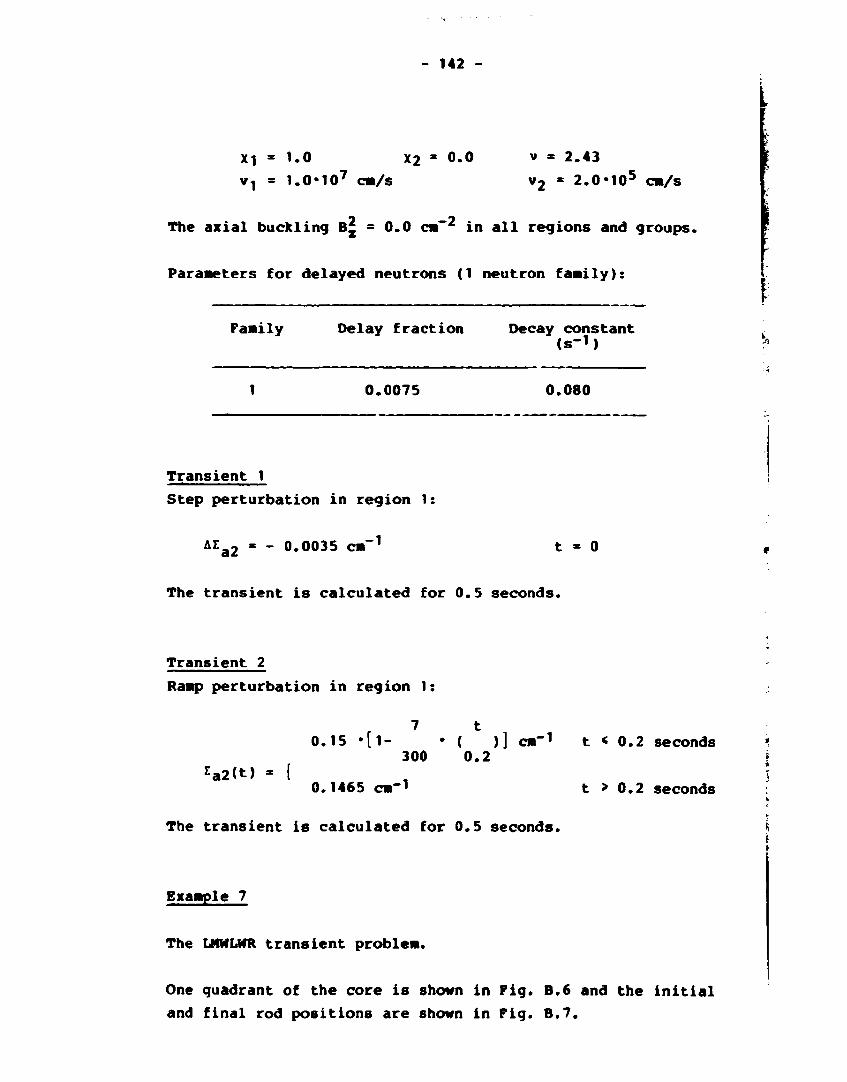
- 142 -

Xi = 1.0 X2 * 0.0 v » 2.43

v1 = 1.0-107 cm/s v2 * 2.0-10

5 cm/s

The axial buckling B2 = 0.0 cm-2 in all regions and groups.

Paraaeters for delayed neutrons (1 neutron family)z

Family Delay fraction Decay constant (s-1)

0.0075 0.080

Transient 1

Step perturbation in region 1:

AEa2 * ~ 0*0035 cm"1 t - 0

The transient is calculated for 0.5 seconds.

Transient 2

Ramp perturbation in region 1:

r 7 t 0.15 »[1- • ( )] cm-1 t < 0.2 seconds

300 0.2 za2(t) - {

0.1465 en"1 t > 0.2 seconds


Example 7

The LMWLVTR transient problem.

One quadrant of the core is shown in Pig. B.6 and the initial

and final rod positions are shown in Pig. B.7.

- 143 -


0 10 30 50 70 90 W) Or

10

30

50

70

90

110

,*., X .

» - 0 . 2

1 HM 7 M >

»od «r*>«2

> " • »>

2

2

Rod 9T««c T 3

4

yfcm)

«(c....

Fig. B.6. One quadrant of the core for the three-dimen

sional LMWLWR benchmark.

z(cm)

Vftical Cross Section

ifcm) 200

180

8

100 4-

60

20

0

*=tf * 2

ami«?

ftod group I

/ V

• " ^ g n u

groupl

gBup 2

Initial rod positions Final rod positions

Fig. B.7. A vertical view of the core for the three-

dimensional LMWLWR benchmark with the initial control

rod pattern at left and the final one at right.

V


- 144 -

Region

1

2

3

4

Group

1

2

1

2

1

2

1

2

°g <c«)

1.423913

0.356306

1.423913

0.356306

1.425611

0.350574

1.634227

0.264002

rag

(car*)

0.01040206

0.08766217

0.01095206

0.09146217

0.01099263

0.09925634

0.002660573

0.04936351

vEfg

(car1)

0.00*477691

0.1127328

0.00647769

0.1127328

0.007503284

0.1378004

0.0

0.0

*21

(car1)

0.0175555

0.0175555

0.01717768

0.02759693

Xi • 1.0 X2 • 0.0

v, = 1.25*107 cm/s v » 2.5

v2 = 2.5»105 c«/s

Parameters Cor delayed neutrons (6 neutron families):

Family

1

2

3

4

5

6

Delay fraction

0.000247

0.0013845

0.001222

0.0026455

0.000832

0.000169

Decay constant

(s"1)

0.0127

0.0317

0.115

0.311

1.40

3.87

Perturbation:

Rod group 1 removed at 3.0 cm/s for 0 < t < 26.666 seconds.

Rod group 2 inserted at 3.0 cn/s fvr 7.5 < t < 7.5 seconds.

The transient is calculated for 60 seconds.

- 145 -

Example 8

The LRABWR two-diaensional benchmark.

One quadrant of the core is shown in Fig. B.8.


0 15 75 105 135 «5

15

\

75

» 5

120

135

165

"X

» y

•a«

xfc«n)

lir

-••yfcmj Fig. B.8. One quadrant of

the core for the two- and

three-dimensional LRABWR

benchmark.


Region

1

2

3,R

4

5

Group

1

2

1

2

1

2

1

2

1

2

D9

(cm)

1.255

0.211

1.268

0.1902

1.259

0.2091

1.259

0.2091

1.257

0.1592

£ag

(cm-1)

0.008252

0.1003

0.007181

0.07047

0.008002

0.08344

0.008002

0.073324

0.0006034

0.01911

v£fg

, -a-1)

0.004602

0.1091

0.004609

0.08675

0.004663

0.1021

0.004663

0.1021

0.0

0.0

*21

(crn-1)

0.02533

0.02767

0.02617

0.02617

0.04754

X1 • 1.0 X2 • 0.0 v » 2.43

- 146 -

The axial buckling B* = 1.0*10 * cm * in all regions and

groups.

Parameters for delayed neutrons (2 neutron families):

Family Delay fraction Decay constant

(s-1)

1 0.0054 0.0654

2 0.001087 1.35

Adiabatic heatup

r - - i 3

«s[zci(r,t)a*,(r,t) + Zf2(r,t)'42(r,t)J - T" T(r,t) 3t

conversion factor: o = 3.83 • 10"^ K • cm^

Doppler feedback

Za1(r,t) » £a1(r,0)[l+Y(/T(rrt) - /TQ)]

feedback constant: Y * 2.034-10-3 R V 2

initial temperature: T 0 = 300 K

Power

P(r,t) - e[zfl(r,!)•,(?,t) • E£2(r,t)*2(f,t)]

energy conversion factor: c » 3.204*10"^ W»s/fission

V

- 147 -

The initial flux distribution shall be normalized such that the

average power density

P = — l(lfl*)+Zf2*2)åv = 1.0 -10~6 W cm"3

Perturbation

Control rod region (R) is given by

0.08344 • (1-0.0606184«t) cnr* for t < 2.0 s Ea2(t))= 1

0.073324 cm-1 for t > 2.0 s


Example 9

The LRABWR three-dimensional benchmark.

Example 9 is the three-dimensional case of example 8. A vertical

view of the core is shown in Pig. B.9.

Perturbation

Control rod region (R) is removed with a velocity of 150 cm/s.

\

- 148 -

9»g

Wftical Cross Stction y=0

360

330

30

n

*m)

5

1 2 3 5

5

r

_xfcm)

0 15 75 105 135 165

Fig. B.9. A vertical picture ot the core for the three-

dimensional LRABWR benchmark. I

- 149 -

APPENDIX C

C.I Solutions to the IAEA-2D benchmark

The reference power distribution is

8

1 0.7456 1.3097 1.4537 1.2107 0.6100 0.9351 0.9343 0.7549

2 1.4351 1.4799 1.3149 1.0697 1.03tl 0.9504 0.7358

3 1.4694 1.3451 1.1792 1.^705 0.9752 0.6921

4 1.1929 0.9670 0.9064 0.8461

5 0.4706 0.6856 0.5972

6 0.5849

kgff » 1.029585

The reference solution is calculated with a nodal program called

MEDIOM-2 with a mesh length of 3 1/3 cm (Wagner, Finnemann,

Koebke, and Winther, 1977).

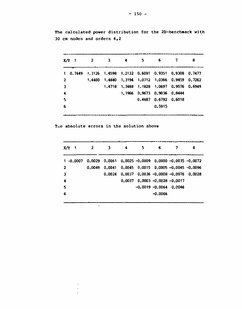
- 150 -

The calculated power distribution for the 2D-benchmark with

30 cm nodes and orders 4,2

XA 1 2 3 4 5 6 7 8

7= '

1 0.7449 1.3126 1.4598 1.2132 0.6091 0.9351 0.9308 0.7477

2 1.4400 1.4840 1.3194 1.0712 1.0366 0.9459 0.7262

3 1.4718 1.3488 1.1828 1.0697 0.9S76 0.6949

4 1.1966 0.9673 0.9036 0.8444

5 0.4687 0.6792 0.6018

6 0.5915

Tne absolute errors in the solution above

X/Y 1

1 -0.0007 0.0029 0.0061 0.0025 -0.0009 0.0000 -0.0035 -0.0072

2 0.0049 0.0041 0.0045 0.0015 0.0005 -0.0045 -0.0096

3 0.0024 0.0037 0.0036 -0.0008 -0.0076 0.0028

4 0.0037 0.0003 -0.0028 -0.0017

5 -0.0019 -0.0064 0.0046

6 -0.0066

- 151 -

C.2. Solutions to the IABA-3P benchmark • • * !• i i • . • • .

The reference assembly power distribution is

X A 1 2 3 4 5 6 7 8 • M . . . • i • ±m- — . » i . • « . - - " ^ - - m LI - i. — • • • — — — . • • • • - — — • , . « . • — » • — • • • • I, ,

1 0.7290 1.2830 1.4230 1.1950 0.6100 0.9340 0.9580 0.7730

2 1.3980 1.4320 1.2920 1.0720 1.0550 0.9740 0.7530

3 1.3690 1.3110 1.1810 1.0880 0.9970 0.7070

4 1.1790 0.9720 0.9230 0.864O 5 0.4750 0.6990 f.60i0

0.5970

kgf f. = 1.02903

The reference so lu t ion i s ca lculated with a nodal program ca l l ed IQSBOX with a node s i z e of 10 * 10 * 10 cm3 (Wagner, Finnemann, Koebke and Winther, 1977).

The calculated assembly power d i s t r i b u t i o n with orders 4,2

X/Y 1

1 0.7348 1.2922 1.4363 1.2001 0.6105 0.9488 0.9499 0.7650

2 1.4108 1.4441 1.2992 1.0722 0.0507 0.9648 0.7428

3 1.3815 1.3185 1.1832 1.0836 0.9864 0.7102

4 1.1829 0.9703 0.9162 0.8605

5 0.4734 0.6903 0.6133 6 0.6024

- 152 -

The absolute errors in the above solution

X/Y 1

1 0.0058 0.0092 0.0133 0.0051 0.0005 -0.0052 -0.0081 -0.0080

2 0.0128 0.0121 0.0072 0.0002 -0.0043 -0.0092 -0.0102

3 0.0125 0.0075 0.0022 -0.0044 -0.0106 0.0032

4 0.0039 -0.0017 -0.0068 -0.0035

5 -0.0016 -0.0087 0.0053

6 0.0054

C.3. Solutions to the Biblis benchmark

BIBLIS-1

1.1190 1.1*9* 1 .155* 1 .165*

1.1290 1.1595 \.1653 1.1875

1.1*51 1.17*5 1.1801 1.1883

23.12CH 11.56Cn 5 .78Cn

T»'£DIfl

1.2716 1.3033 1 .309 ; 1,3183

1.1603 1.1876 1.1926 1.2117

1.1*56 1.1689 1.1730 1.1760

1.2*78 1.2735 1.2782 1.29*3

1.2*81 1.2733 1.2777 1.2823

1.1237 1.1*15 1.1**6 1.1559

1.1727 1.18*2 1.1859 1.1808

1.109* 1.1270 1.1302 1.1319

1.0856 1.1017 1.10*6 1.1163

1.1326 1.1*37 1.1*5* 1.1*19

1.0*16 1.0*15 1 .0*1* 1.0*2*

1.1097 1.0970 1.09*2 1.0792

0 . 9 9 6 9 1 .0066 1 .0086 1 .0190

1.0*55 1 .0531 1 .05*7 1 .05*3

0 . 9 2 8 2 0 . 9 2 9 5 0 . 9 2 9 7 0 . 9 3 3 5

0 . 9 * 2 5 0 . 9 3 0 6 0 . 9 2 8 2 0 . 9 1 6 2

0 . 9 7 1 9 0 . 9 * 0 7 0 . ° 3 5 * 0 . 9 2 2 2

1.1*26 1 .090* 1 .0790 1 .0559

1.1085 1.1126 1.1137 1.1158

1.08*1 1.0838 1.08*2 1.0857

0 .9325 0 .9231 0 .9218 0 .9169

0 .7*52 0 .7231 0 .7181 0 .7130

0 .8227 0 .7877 0 .7806 0 .76*8

0 . 6 1 9 * 0 .5908 0 . 5 8 * 9 0 .5699

1.1095 1.0222 1.0232 1.0283

0 .9726 C.9723 0 . 9 7 2 7 0 .9762

0 .6233 0 .8077 0 .8062 0 .8055

0 .5061 O.*900 0 .*87* O.*830

- 153 -

BIBLIS-2

1.6130 1.6*62 1 .653* 1 .6685

1 .6061 1 .6393 1.6*62 1.6685

1.6101 1.6*18 1.6*8* 1.6611

23.12CM 11.56CM 5.78CH

TVEDIM

1.7*03 1.77** 1 .7812 1.7952

1 .5709 1.5998 1.6057 1.6327

l . * 9 9 8 1.52*3 1 .5289 1.53*3

1.59*5 1.6213 1.6266 1.6*87

1.5790 1.605* 1.6103 1.6176

1.3813 1.3992 l . * 0 2 5 1.4175

1.3777 1.3882 1.3897 1.38**

1.2569 1.2753 1.2787 1.2818

1.21*8 1.2309 1.2338 1.2*78

1.2*29 1.2532 1.25*9 1.2512

1.1292 1.1273 1.1269 1.1272

1.1761 1.1599 1.1563 1.1380

0 . 9 2 * 5 0 . 9 3 * 3 0 . 9 3 6 1 0 . 9 * 5 7

0 . 9 3 0 2 0 . 9 3 7 7 0 . 9 3 9 0 0 . 9 3 8 1

0 . 7 7 9 9 0 . 7 8 2 2 0 . 7 8 2 * 0 . 7 8 3 6

0 . 8 7 5 6 0 . 8 6 2 5 0 . 8 5 9 7 0 . 8 * 5 9

0 . 9 8 0 6 0 . 9 * 5 5 0 . 9 3 9 2 0 . 9 2 2 1

1 .1791 1 .117* i . l 0 * 3 1 .0751

0 .8*37 0 . 8 * 7 0 0 .8*79 0 .8*81

0 .7350 0 .7370 0 .7375 0 . 7 3 6 1

0 .4180 0 .4137 0 .*129 0 .4130

0 .5376 0 .5180 0 .5135 0 .5055

0 .7826 0 .7*32 0 .735* 0 .7156

0 .63*9 0 .5992 0 .5922 0 .5736

0 .71*6 0 . 7 1 6 * 0 .7170 0 .7190

0 .6220 0 .6219 0 .6220 0 .622*

0 .**08 0 .*29* 0 .4282 0 .4246

0 .3066 0 .2933 0 .2913 0 .2867

BIBLIS-3/1

1.0855 1.0938 1.09*5 1.09*6

1.0962 1.10*8 1.1055 1.09*1

1.1129 1.1206 1.1211 1.1212

23.12Crt 11 .56 CM 5.78CM

THODIM

1.2378 1.2*63 1.2*68 1.2*6*

1.1308 1.1379 1.1381 1.127*

1.120* 1.126* 1.1258 1.1269

1.2169 1.22*8 1.22*3 1.2167

1.2212 1.2280 1.2271 1.2286

1.10*9 1.1100 1.108* 1.1002

1.1620 1.1661 1.1635 1.1660

1 .0885 1 .0921 1.0905 1 .09*2

1.0675 1 .0716 1.0698 1 .0632

1 .1209 1 .12*5 1 .1219 1 .125*

1 .0423 1 .0*25 1.0401 1.0344

1 .1269 1 .12*2 1 .1225 1.1265

0 . 9 6 2 7 0 . 9 8 2 3 0 . 9 8 1 5 0 . 9 7 7 9

1 .0333 1.0326 1 .0313 1.0366

0 . 9 2 5 5 0 . 9 2 5 3 0 . 9 2 3 5 0 . 9 2 0 1

0 . 9 5 * 3 0 . 9 5 1 3 0 . 9 * 9 5 0 . 9 5 * 8

1.0017 0 . 9 9 1 7 0 . 9 9 1 7 0 .9920

1.2080 1.19*3 1.1967 1.2009

1.0956 1.089* 1.0911 1.0993

1.07*5 1.0676 1.0686 1.075*

0.93*6 0 .9286 0 .9285 0.9357

0 .7689 0.7637 0 .7636 0.7631

0 .8728 0 .8711 0 .8725 0 .87*3

0 .6764 0.6794 0 .6825 0 .6838

1.0091 1.0052 1.0099 1.0168

0 .965* 0 .962* 0 .9663 0 .9727

0 .8235 0 .8193 0 .821* 0 .8261

0 .5*12 0 .5*27 0 .5*38 0 .5*57

- 154 -

BIBLIS-3/2

1.0875 1.0950 1.09*9 1.07**

1.0980 1.1060 1.1057 1.0975

1.11*7 1.1217 1.1213 1.1010

23.12CN 11.56 CH S.78CH

TVEDIM

1.2395 1.2*73 1.2*66 1.2267

1.1323 1.138* 1.1378 1.1309

1.1215 1.1262 1.1252 1.1076

1.2200 1.22*7 1.2237 1.2165

1.2223 1.227* 1.226* 1.2100

1.1055 1.1085 1. 107* 1. 10*2

1. 1622 1.1635 1.1622 1. 1501

1 .0889 1 .0907 1 .0899 1 .078*

1 .0679 1.0699 1 .0691 1 .0691

1.1210 1.1220 1.1209 1.1109

1.0*20 1.0*00 1 .0391 1.0*20

1.1262 1.1225 1.1217 t . 1 1 8 9

0 . 9 8 2 6 0 . 9 8 1 6 0 . 9 8 1 6 0 . 9 8 7 *

1.0331 1.0315 1.0312 1.0278

0 . 9 2 5 3 0 .9235 0 .9232 0 . 9 2 8 5

0 .9537 0 .9*96 0 . 9 * 9 1 0 . 9 * 6 *

1.0007 0 . 9 9 1 5 0 . 9 9 1 * 0 . 9 9 7 *

1.2066 1.1963 1.1968 1.2065

1.0953 1.0917 1.0923 1.0965

1.07*1 1.0692 1.0696 1.07*5

0 . 9 3 * 1 0 . 9 2 8 8 0 . 9 2 9 1 0 . 9 3 1 2

0 . 7 6 8 3 0 . 7 6 3 3 0 . 7 6 3 7 0 . 7 7 2 0

0 . 8 7 1 9 0 . 8 7 1 8 0 . 8 7 2 7 0 . 8 8 1 *

0 . 6 7 5 5 0 . 6 8 1 1 0 . 6 8 2 7 0 . 6 9 1 8

1.0089 1 .0098 i . O l l S 1 .0256

0 . 9 6 5 2 0 . 9 6 6 2 0 . 9 6 8 1 0 . 9 8 1 1

0 . 8 2 3 1 0 . 8 2 1 2 0 . 8 2 2 7 0 . 8 3 3 1

0 . 5 * 0 9 0 . 5 * 3 3 0 . 5 * * * 0 . 5 5 2 0

BIBLIS-4/1

1.5752 1.5818 1.5823 1.5859

1.569* 1.576* 1.5768 1.5653

1.57*3 1.5802 1.580* 1.585*

23.12CH 11.56CH 5.78CH

TUODin

1.7032 1.7100 1.7101 1.71*7

1.5388 1.5*37 1.5*37 1.5339

1.4730 l . * 7 6 5 l . * 7 6 1 1.*817

1.56*1 1.5676 1.5673 1 .5603

1.5509 1.5552 1.55*9 1.5593

1.3621 1.36*0 1 .363* 1 .355*

1.367* 1.3675 1.3666 1.3715

1.236* 1.2387 1 .2383 1.2*30

1.1972 1.1990 1.1986 1.1917

1.2320 1.2323 1.2316 1.2360

1.1308 1.1278 1.1272 1.1215

1.19*5 1.1892 1.186* 1.1927

0 . 9 1 2 * 0 . 9 1 3 1 0 .9130 0 . 9 0 8 3

0 . 9 2 0 1 0 . 9 1 9 7 0 . 9 1 9 * 0 .9232

0 . 7 7 8 * 0 . 7 7 8 5 0 . 7 7 8 3 0 . 7 7 5 5

0 . 8 8 7 7 0 . 8 8 3 * 0 . 8 8 2 8 0 . 8 8 7 2

1.0108 0 . 9 9 9 3 0 . 9 9 9 1 0 . 9 9 6 6

1.2**3 1.2290 1.2293 1.2322

0 . 8 3 * 7 0 . 8 3 3 3 0 . 8 3 3 * 0 . 8 3 7 0

0 . 7 2 9 0 0 . 7 2 8 6 0 . 7 2 8 7 0 . 7 3 2 *

0 . * 2 1 0 0 . * 2 0 0 0 . * 2 0 0 0 . * 1 8 2

0 . 5 5 9 9 0 . 5 5 6 * 0 . 5 5 6 6 0 . 5 5 6 1

0 . 8 2 * 6 0 . 8 2 1 * 0 . 8 2 2 0 0 . 8 2 2 8

0 . 6 8 9 2 0 . 6 9 1 3 0 . 6 9 2 8 0 . 6 9 3 2

0 . 7 0 6 9 0 . 7 0 9 3 0 . 7 1 0 * 0 . 7 1 3 1

0 . 6 1 8 2 0 . 6 2 0 9 0 . 6 2 1 8 0 . 6 2 * 6

0 .***6 0 . * * 5 5 0 . * * 6 2 0 .**90

0 . 3 * 2 8 0 . 3 * * 8 0 . 3 * 5 * 0 . 3 * 6 0

- 155 -

BIBLIS-4/2

1.5724 1.5798 1.5806 1.5638

1.5666 1.5745 1.5752 1.5757

1.5716 1.5784 1.5789 1.5620

2 3 . 1 2 CM 11.56 CD 5.78CM

TVEDIM

1.7005 1.7082 1.7086 1.6926

1.5365 1.5422 1.5424 1.5431

1 . 4 7 U 1 .4753 1.4751 1.4602

1.5620 1 .5663 1 .5662 1.5647

1.5490 1.5540 1.5538 1.5403

1 .3609 1 .3632 1.3628 1.3643

1.3670 1.3672 1 .3663 1 .3562

1.2352 1.2380 1.2377 1.2273

1.1962 1.198« 1.1981 1.2004

1.2316 1.2320 1.2313 1.2223

1.1313 1.1280 1.1273 1.1323

1.1961 1.1900 1.1890 i . 1 8 7 7

0 .9120 0 .9130 0 .9129 0 .9168

0 .9198 0 .9196 0 .9193 0 .9143

0 .7785 0 .7786 0 .7784 0 .7806

0 .8887 0 .8840 0 .8832 0 .8807

1.0129 1.0004 0 .9999 1.0069

1.2476 1.2308 1.2306 1.2421

0 .8349 0 .8336 0.8337 0 .8335

0 .7293 0 .7290 0 .7290 0 .7282

0 .4213 0 .4203 0 .4203 0 .4237

0 .5609 0 .5570 0 .5570 0 .5616

0 .8267 0 .8226 0 .8229 0 .3314

0 .6912 0 .6925 0 .6937 0 .7036

0 . 7 0 7 5 0 . 7 1 0 1 0 . 7 1 1 2 0 . 7 1 7 6

0 . 6 1 8 9 0 . 6 2 1 6 0 . 6 2 2 5 0 . 6 2 7 9

0 . 4 4 5 3 0 . « 4 6 1 0 . 4 4 6 8 0 . 4 4 9 8

0 .3435 0 .3454 0 . 3 4 5 9 0 . 3 5 0 1

BIBLIS with new albedos

1.0814 1.1084 1.1136 1.0744

1.0921 1.1193 1.1243 1.0975

1.1089 1.1349 1.1397 1,1010

23.12CM 1!,56CH 5.78CH

TVEOIH

1.2334 1 .2617 1 .2667 1.2267

1 .1269 1 .1512 1 .1556 1 .1309

1 .1168 1 .1376 1 .1412 1.1076

1.2150 1.2379 1.2420 1.2165

1.2175 1.2400 1.2438 1.2100

1.1018 1.1178 1.1206 1.1042

1.1595 1.1701 1.1716 1.1501

1.0859 1.1016 1.1044 1.0784

1.0650 1.0795 1.0820 1.0691

1.1186 1.1287 1.1303 1.1109

1.0411 1.0413 1.0413 1.O420

1.1279 1.1172 1,1149 1.1189

0 .9820 0 .9906 0.9924 0.9874

1.0325 1.0393 1.0407 1.0278

0 .9245 0.9257 0 .9259 0 .9285

0 .9543 0 .9432 0.9411 0.9464

1.0058 0 .9780 0 .9735 0.9974

1.2200 1.1745 1.1651 1.2065

1.0974 1.1010 1.1019 1.0965

1.0766 1.0760 1.0763 1.0745

0 .9364 0 .9273 0 .9260 0 .9312

0 .7650 0 .7449 0 .7402 0 .7720

0 .8635 0 .8335 0 .8279 0 . 8 8 1 *

0 .6921 0 .6667 0 .6619 0 .6916

1.0136 1.0159 1.0167 1.0256

0 .9705 0 . 9 6 9 9 0 . 9 7 0 2 0 . 9 8 1 1

0 .8321 0 .8177 0 .8161 0 . 8 3 3 1

0.540.'! 0 . 5 2 4 6 0 .5218 0 .5520

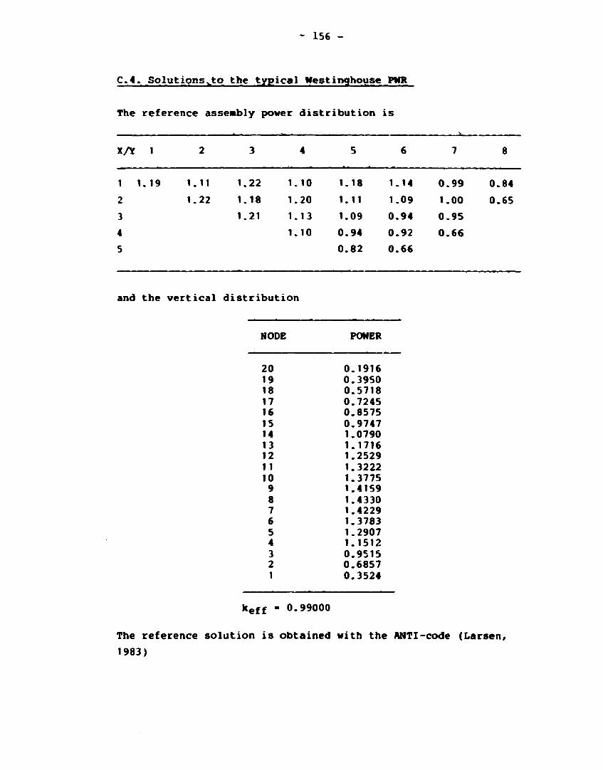
- 156 -

C.4. Solutions^to the typical Westinghouse PWR

The reference assembly power distribution is

xA i

1 1.19

3

4

5

2

1-11

1.22

3

1.22

1.18

1.21

4

1 .10

1.20

1.13

1.10

5

1.18

1.11

1.09

0 .94

0 . 8 2

6

1.14

1.09

0 .94

0 . 9 2

0 . 6 6

7

0 . 9 9

1 .00

0 . 9 5

0 . 6 6

8

0 .84

0 .65

and the vertical distribution

NODE

20 19 18 17 16 15 14 13 12 11 10

9 8 7 6 5 4 3 2 1

POWER

0 .1916 0 .3950 0 .5718 0 .7245 0 .8575 0 .9747 1.0790 1.1716 1.2529 1.3222 1.3775 1.4159 1.4330 1.4229 1.3783 1.2907 1.1512 0 .9515 0 . 6 8 5 7 0 .3524

keff - 0.99000

The reference solution is obtained with the ANTI-code (Larsen,

1983)

- 157 -

The calculated assembly powers for example 4 by use of the

reflector parameters calculated by Thorlaksen (1981). The node

size = 21.5 * 21.5 * 18.3 cm3.

X A 1 2

1 1.03 1.00

1.00 0 . 9 8

1 .02 0 . 9 9

1.19 1.11

2 1.07

1.05

1 .07

1 .22

3

4

5 NEM w i t h o§

MEN w i t h <xT

QUANDRY

ANTI ( r e f e r e n c e )

3

1.09

1.07

1.09

1.22

1.09

1.07

1.09

1.18

1.12

1.11

1.12

1.21

4

1.06

1.05

1.06

1.10

1.13

1.11

1.13

1.20

1.11

1.09

1.10

1.13

1.09

1.08

1.08

1.10

5

1.17

1.16

1.17

1.18

1.13

1.12

1.13

1.11

1.10

1.09

1.10

1.09

0 . 9 9

0 .98

0 . 9 8

0 .94

0 .88

0 . 8 9

0 . 8 8

0 . 8 2

6

1.22

1.21

1.21

1.14

1.15

1.15

1.15

1.09

1.01

1.02

1.01

0 .94

0 .94

0 .94

0 .94

0 . 9 2

0 .66

0 . 6 8

0 . 6 7

0 . 6 6

7

1.11

1.12

1.10

0 . 9 9

1.06

1.07

1.06

1.00

0 . 9 4

0 . 9 6

0 . 9 5

0 . 9 5

0 . 6 3

0 . 6 5

0 . 6 5

0 . 6 6

8

0 .94

0 . 9 7

0 . 9 5

0 . 8 4

0 . 6 9

0 . 7 1

0 . 7 1

0 . 6 5

The eigenvalues are

NEM a£

NEM aT

QUANDRY

ANTI

0.99399

0.99443

0.99417

0.99000

- 158 -

The calculated assembly powers for example 4 with new albedo

representat ion.

XA 1 2

1 0.99 0.97

0.96 0.94

1.19 1.11

2 1.04

1.01

1.22

3

4

3

1.06

1.03

1.22

1.06

1.03

1.18

1.07

1.05

1-21

5 NEM with new albedos

NEM with cross sections

ANTI (reference)

4

1.04

1.02

1.10

1.11

1.08

1.20

1.09

1.07

1.13

1.08

1.07

1.10

5

1.16

1.14

1.18

1.13

1.11

1.11

1.10

1.08

1.09

0.99

0.99

0.94

0.90

0.92

0.82

6

1.22

1.20

1.14

1.15

1.14

1.09

1.03

1.02

0.94

0.96

0.98

0.92

0.68

0.77

0.66

7

1.10

1.08

0.99

1.08

1.08

1.00

0.97

1.01

0.95

0.66

0.71

0.66

8

0.96

0.94

0.84

0.71

0.75

0.65

The eigenvalues are

NEM Albedo 0.99461

NEM cross sections 0.99509

ANTI 0.99000

- 159 -

C.5 Solutions to the infinite slab »odel — ^ » — • • • • — M l — I. — — — ^ ^ | — ^ — ^ ^ —

Infinite slab reactor »odel. +3% theraal absorption cross

section in region 1 in 1.0 second.

Tiæ Sec.

0.0

0.1

0.2

0.3

0.4

0.5

0.6

0.7

0.8

0.9

1.0

1.5

2.0

Relative regional Region 1 Region 2

1.000

0.859

0.747

0.656

0.586

0.523

0.477

0.433

0.397

0.362

0.339

0.316

0.298

1.000

0.929

0.875

0.828

0.792

0.760

0.735

0.712

0.692

0.672

0.660

0.639

0.619

power Region 3

1.000

0.989

0.982

0.969

0.962

0.955

0.947

0.941

0.936

0.930

0.925

0.909

0.891

Total power

1.000

0.926

0.869

0.819

0.782

0.748

0.722

0.698

0.678

0.658

0.644

0.624

0.605

Total power (reference)

1.000

0.930

0.873

0.760

0.659

0.643

0.631

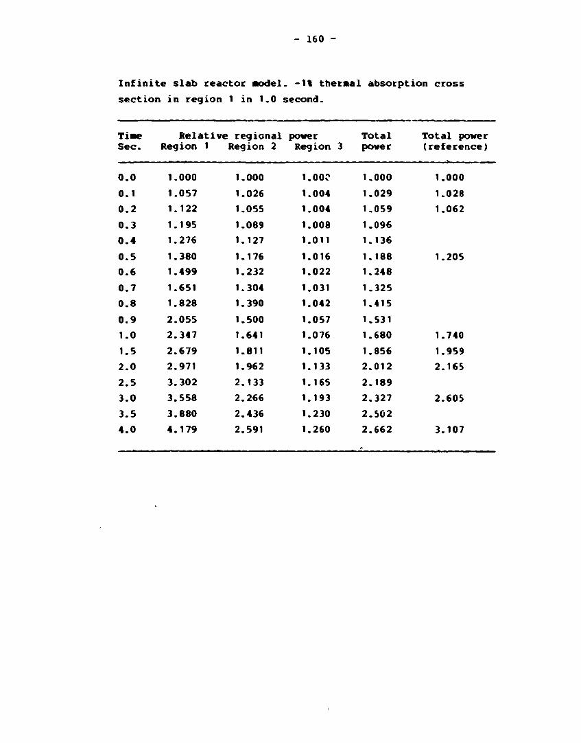
- 160 -

Infinite slab reactor aodel. -1% thermal absorption cross

section in region 1 in 1.0 second.

Tiae Relative regional potter Total Total powe Sec. Region 1 Region 2 Region 3 power (reference

0 . 0

0 . 1

0 . 2

0 . 3

0 . 4

0 . 5

0 . 6

0 . 7

0 . 8

0 . 9

1.0

1.5

2 . 0

2 . 5

3 . 0

3 . 5

4 . 0

1.000

1.057

1.122

1.195

1.276

1.380

1.499

1.651

1.828

2 .055

2 . 3 4 7

2 . 6 7 9

2 . 9 7 1

3 .302

3 .558

3 .880

4 . 1 7 9

1.000

1.026

1.055

1.089

1.127

1.176

1.232

1.304

1.390

1.500

1.641

1.811

1.962

2.133

2.266

2.436

2.591

1.00?

1.004

1.004

1.008

1.011

1.016

1.022

1.031

1.042

1.057

1.076

1.105

1.133

1.165

1.193

1.230

1.260

1.000

1.029

1.059

1.096

1.136

1.188

1 .248

1.325

1.415

1.531

1.680

1.856

2 . 0 1 2

2 . 1 8 9

2 . 3 2 7

2 . 5 0 2

2 . 6 6 2

1.000

1.028

1.062

1.205

1.740

1.959

2 .165

2 .605

3.107

- 161 -

Infinite slab reactor model. -5% thermal absorption cross

section in region 1 in 0.01 seconds.

Time Sec.

0.000

0.001

0.002

0.003

0.004

0.005

0.008

0.010

0.012

0.015

0.018

0.020

Relative Region 1

1.000

1.064

1.216

1.470

1.875

2.507

9.234

35.19

163.1

1582

1.528-

6.934*

104

104

> regional Region 2

1.000

1.015

1.066

1.160

1.313

1.551

3.966

12.68

56.34

542.3

5239

2.375-10*

power Region 3

1.000

1.002

1.003

1.005

1.011

1.019

1.106

1.342

2.403

15.97

136.7

I 619.6

Total power

1.000

1.025

1.090

1.203

1.385

1.669

4.636

15.79

71.05

685.0

6620

3.000-104


1.000

1.022

1.659

15.65

70.18

680.2

6611

3.011-104

Infinite slab reactor model. -5% thermal absorption cross

section in region 1 in 0.01 seconds. Hot case.

Time Sec.

0.000

0.001

0.002

0.003

0.004

0.005

Relative Region 1

1.000

1.354

2.109

4.573

40.57

3.175« 105

( regional Region 2

1.000

1.168

1.527

2.694

19.44

1.394« •10!

power Region

1.000

1.025

1.073

1.226

3.233

> 1.275«

3

-104

Total power

1.000

1.180

1.562

2.809

20.81

1.537M05


1.000

1.178

1.558

2.797

20.72

1.537-105

- 162 -

C.6 Solutions .to the TWIGL example

The steady-state power solution

X A 1 2 3 4 5 6 7 8 9 10

1 1.258 1.293 1.243 2.373 2.176 1.967 1.691 0.647 0.422 0.139

2 1.321 1.259 2.380 2.161 1.941 1.663 0.635 0.414 0.136

3 1.198 2.350 2.123 1.833 1.602 0.609 0.3% 0.130

4 2.187 2.033 1.779 1.500 0.568 0.368 0.121

5 1.870 1.614 1.350 0.509 0.329 0.108

6 1.380 1.148 0.432 0.279 0.091

7 0.948 0.343 0.220 0.072 8 0.260 0.157 0.051

9 0.093 0.030 10 0.010

kgff = 0.91318

Normalized power distribution for TWIGL with ramp-perturbation to

different times

T = 0.0 seconds

X A 1 2 3 4 5 6 7 8 9 10

1 1.258 1.293 1.243 2.373 2.176 1.967 1.691 0.647 0.422 0.139

2 1.321 1.259 2.380 2.161 1.941 1.663 0.635 0.414 0.136

3 1.198 2.350 2.123 1.883 1.602 0.609 0.396 0.130

4 2.187 2.033 1.779 1.500 0.568 0.368 0.121

5 1.870 1.614 1.350 0.509 0.329 0.108

6 1.380 1.148 0.432 0.279 0.091

7 0.948 0.343 0.220 0.072 8 0.260 0.157 0.051 9 0.093 0.030

10 0.010

- 163

T = 0 . 0 5 s e c o n d s

X / V 1 2 3 4 5 6 7 8 9 10

1 1.251 1.286 1.237 2.362 2.167 1.959 1.685 0.645 0.420 0.138

2 1.314 1.253 2.371 2.155 1.936 1.658 0.663 0.412 0.135

3 1.193 2.346 2.121 1.883 1.602 0.609 0.395 0.130

4 2.194 2.044 1.790 1.509 0.569 0.368 0.121

5 1.885 1.629 1.362 0.511 0.330 0.108

6 1.394 1.160 0.434 0.280 0.092

7 0.957 0.346 0.221 0.072

8 0.261 0.158 0.052

9 0.093 0.031

10 0.01O

T = 0 . 1 0 s econds

XA i

1 1.243

2

3

4

5

6

7

8

9

10

2

1.278

1.307

3

1.230

1.247

1.189

4

2.351

2.361

2.341

2.201

5

2.157

2.147

2.119

2.054

1.899

6

1.951

1.930

1.882

1.801

1.643

1.409

7

* • •

1.678

1.654

1.601

1.518

1.374

1.172

0.968

8

0.643

0.632

0.609

0.571

0.514

0.437

0.348

0.263

9

0.419

0.411

0.395

0.369

0.331

0.282

0.222

0.158

0.094

10

0.138

0.135

0.129

0.121

0.108

0.092

0.073

0.052

0.031

0.010

- 164 -

T = 0 . 1 5 seconds

X A " 2 3 4 5 6 7 8 9 10

» m H M , I , , I I 1 • • - , - i i l - i i • i i • • . - _ - . • • - - - - - _ , - , , , • • • ! • • • • •

1 1.235 1.271 1.223 2.338 2.147 1.942 1.671 0.640 0.418 0.137

2 1.299 1.241 2.351 2.139 1.924 1.649 0.630 0.410 0.135

3 1.184 2.336 2.117 1.882 1.601 0.608 0.395 0.129

4 2.208 2.065 1.812 1.527 0.572 0.369 0.121

5 1.914 1.659 1.387 0.516 0.332 0.109

6 1.424 1.185 0.440 0.283 0.092

7 0.978 0.351 0.224 0.073

8 0.265 0.159 0.052

9 0.C94 0.031

10 0.010

T = 0 . 2 0 seconds

X A 1 2 3 4 5 6 7 8 9 10

1 1.227 1.263 1.216 2.326 2.137 1.934 1.665 0.638 0.416 0.137

2 1.292 1.234 2.341 2.131 1.918 1.644 0.628 0.409 0.134

3 1.180 2.330 2.115 1.881 1.601 0.608 0.395 0.129

4 2.215 2.C75 1.823 1.537 0.574 0.370 0.121

5 1.930 1.674 1.400 0.519 0.334 0.109

6 1.439 1.198 0.443 0.284 0.093

7 0.989 0.353 0.225 0.074

8 0.267 0.160 0.052

9 0.095 0.031

10 0.010

- 165

T = 0 .2b - 0 . 5 0 s econds

XA I 2 3 4 5 6 7 8 9 10

' ^ ' • • — ' • • ' — • • • • " * T • ~ • • • I I - - II — ! • - • • - - • — , , , — — — — , . . . ^ . _ , — . - —

1 1,228 1.263 1.217 2.326 2.136 1.934 1.664 0.638 0.416 0.137

2 1.293 1.235 2.341 2.131 1.917 1.64«! 0.628 0.409 0.134

3 1.180 2.330 2.115 1.881 1.601 ?.608 0.395 0.129

4 2.214 2.075 1.822 1.537 0.574 0.370 0.121

5 1.929 1.674 1.400 0.519 0.334 0.109

6 1.439 1.198 0.443 0.285 0.093

7 0.989 0.353 0.225 0.074

8 0.267 0.160 0.053

9 0.095 0.031

10 0.010

C./. Solutions to the LMWLWR transient problem

The steady-state assembly power distribution obtained by NBH of

orders 4,2.

X A i

1 1.560

2

3

4

2

1.476

1.417

3

1.283

1.244

1.126

- i . _ i -

4

0.982

0.964

0.873

0.763

/

5

0.642

0.626

0.554

0.380

keff = 0.99953

- 166 -

C . 8 . _ S o l u t i o n s t o the LRABWR two-d imens iona l benchmark

The s t e a d y - s t a t e power d i s t r i b u t i o n for t h e r o d - i n s i t u a t i o n ob

t a i n e d by NEM of o r d e r s 4 , 2 and a node s i z e o f 15 * 15 cm2.

XA 1 2 3 4 5 6 7 8 9

1 0.6360 0.4538 0.4230 0.5208 0.8012 1.4082 1.6848 1.4925 0.9244

2 0.4538 0.4107 0.4157 0.4986 0.6795 0.9492 1.1591 1.2876 0.8663

3 0.4230 0.4157 0.4316 0.4985 0.6238 0.7866 0.9688 1.1727 0.8222

4 0.5208 0.4986 0.4985 0.5570 0.6806 0.8424 1.0185 1.2148 0.8440

5 0.8012 0.6795 0.6238 0.6806 0.8634 1.1454 1.3286 1.4092 0.9189

6 1.4082 0.9492 0.7866 0.8424 1.1454 1.8445 2.0382 1.6592 0.9520

7 1.6848 1.1591 0.9688 1.0185 1.3286 2.0382 2.1417 1.5931 0.8263

8 1.4925 1.2876 1.1727 1.2148 1.4092 1.6592 1.5931 1.2986

9 0.9244 0.8663 0.8222 0.8440 0.9189 0.9520 0.8263

kgff = 0.99619

The s t e a d y - s t a t e power d i s t r i b u t i o n for the r o d - o u t s i t u a t i o n i n

c o l d s t a t e (no h y d r a u l i c feedback)

XA 1 2 3 4 5 6 7 8 9

1 0.2052 0.1533 0.1543 0.1997 0.3102 1.5443 0.6543 0.5854 0.3670

2 0.1589 0.1532 0.1691 0.2161 0.3005 \4165 0.5107 0.5765 0.3914

3 0.1733 0.1823 0.2114 0.2702 0.3579 0.4594 0.5644 0.6774 0.4729

4 0.2447 0.2545 0.2959 0.3873 0.5274 0.6822 0.8173 0.9448 0.6417

5 0.4078 0.3833 0.4301 0.5845 0.8666 1.2260 1.4088 1.4262 0.8915

6 0.7473 0.5653 0.6053 0.8530 1.4034 2.4385 2.6806 2.0683 1.1233

7 0.9244 0.7274 0.8118 1.1736 1.9685 3.4210 3.5900 2.4560 1.1556

8 0.8452 0.8500 1.0381 1.5202 2.4758 4.0898 4.0068 2.5301

9 0.5373 0.5891 0.7515 1.1065 1.7659 2.7687 2.5553

k e f f * 1.01508

- 167 -

Normalized power distribution to time = 0.4 second. Average power

density * 1.38»10-6 W/cm3

XA 1 2 3 4 5 6 7 8 9

*

1 0.564 0.404 0.380 0.472 0.727 1.283 1.536 1.359 0.843

2 0.405 0.370 0.377 0.457 0.626 0.872 1.066 1.189 0.799

3 0.384 0.380 0.399 0.467 0.588 0.744 0.917 1.109 0.778

4 0.481 0.464 0.471 0.537 0.665 0.829 1.001 1.190 0.825

5 0.746 0.641 0.600 0.673 0.875 1.171 1.357 1.435 0.931

6 1.322 0.899 0.766 0.851 1.191 1.949 2.156 1.743 0.995

7 1.587 1.103 0.953 1.046 1.419 2.231 2.348 1.730 0.889

8 1.408 1.235 1.161 1.261 1.545 1.933 1.872 1.469 0.000

9 0.875 0.832 0.816 0.879 1.016 1.139 0.9% 0.000 0.000

Time = 0.8 seconds. Average power dens i ty = 2.94»10~6 w/cm3

XA 1 2 3 4 5 6 7 8 9

1 0.479 0.345 0.328 0.409 0.632 1.114 1.335 1.183 0.736

2 0.348 0.320 0.330 0.403 0.553 0.771 0.942 1.054 0.710

3 0.337 0.337 0.359 0.426 0.541 0.686 0.845 1.022 0.716

4 0.431 0.421 0.437 0.510 0.643 0.808 0.975 1.154 0.797

5 0.678 0.591 0.570 0.663 0.886 1.201 1.391 1.459 0.940

6 1.209 0.835 0.740 0.862 1.250 2.075 2.294 1.837 1.041

7 1.459 1.033 0.933 1.082 1.540 2.480 2.610 1.894 0.957

8 1.300 1.165 1.146 1.322 1.728 2.312 2.245 1.673 0.000

9 0.810 0.789 0.811 0.931 1.158 1.409 1.252 0.000 0.000

- 168 -

Ti«e « 1.2 seconds. Average power density - 2.34*10~* W/c«3

X A 1 2 3 4 5 6 7 8 9

1 0.372 0.271 0.262 0.331 0.511 0.899 1.079 0.959 0.597

2 0.276 0.257 0.271 0.335 0.461 0.641 0.785 0.880 0.594

3 0.278 0.282 0.308 0.373 0.480 0.610 0.752 0.907 0.635

4 0.367 0.365 0.392 0.474 0.613 0.777 0.937 1.100 0.756

5 0.589 0.524 0.529 0.647 0.896 1.233 1.425 1.478 0.942

6 1.059 0.751 0.705 0.873 1.323 2.232 2.464 1.950 1.088

7 1.287 0.939 0.904 1.128 1.697 2.804 2.950 2.100 1.034

8 1.155 1.069 1.123 1.401 1.974 2.834 2.761 1.945 0.000

9 0.724 0.728 0.799 0.996 1.348 1.790 1.614 0.000 0.000

Tine = 1.4 s e c o n d s . Average power d e n s i t y = 9 . 1 1 W/cm3

X/V 1 2 3 4 5 6 7 8 9

1 0.328 0.241 0.235 0.297 0.460 0.807 0.968 0.862 0.537

2 0.246 0.231 0.246 0.306 0.4^1 0.585 0.716 0.803 0.542

3 0.252 0.258 0.285 0.349 0.452 0.576 0.708 0.853 0.5%

4 0.339 0.340 0.371 0.456 0.597 0.759 0.914 1.069 0.731

5 0.547 0.493 0.509 0 637 0.896 1.240 1.431 1.475 0.935

6 0.986 0.709 0.6B5 0.875 1.351 2.291 2.527 1.988 1.102

7 1.202 0.892 0.887 1.145 1.767 2.952 3.103 2.189 1.065

8 1.083 1.021 1.108 1.435 2.092 3.106 3.030 2.076 0.000

9 0.680 0.697 0.790 1.024 1.442 1.994 1.807 0.000 0.000

- 169 -

Time = 1.6 s e c o n d s . Average power d e n s i t y = 154 W/ci»3

XA 1 2 3 4 5 6 7 8 9

1 0.374 0.270 0.257 0.319 0.485 0.846 1.010 0.897 0.560

2 0.275 0.255 0.265 0.323 0.439 0.605 0.737 0.826 0.559

3 0.274 0.277 0.301 0.361 0.460 0.580 0.710 0.856 0.601

4 0.357 0.355 0.381 0.459 0.591 0.744 0.892 1.046 0.720

5 0.566 0.505 0.514 0.631 0.872 1.1% 1.375 1.421 0.907

6 1.010 0.721 0.685 0.859 1.309 2.208 2.428 1.909 1.064

7 1.226 0.902 0.884 1.125 1.726 2.884 3.024 2.123 1.035

8 1.102 1.031 1.107 1.420 2.076 3.146 3.068 2.060 0.000

9 0.694 0.707 0.794 1.022 1.453 2.065 1.879 0.000 0.000

Time = 1.8 s e c o n d s . Average power d e n s i t y = 341 w/cm3

XA 1 2 3 4 5 6 7 8 9

1 0.329 0.239 0.229 0.285 0.433 0.754 0.901 0.801 0.501

2 0.244 0.228 0.239 0.293 0.398 0.548 0.667 0.748 0.507

3 0.247 0.251 0.276 0.335 0.429 0.542 0.664 0.799 0.560

4 0.326 0.328 0.358 0.439 0.571 0.722 0.864 1.009 0.693

5 0.522 0.472 0.491 0.617 0.866 1.195 1.372 1.410 0.8%

6 0.936 0.677 0.662 0.855 1.329 2.259 2.481 1.339 1.074

7 1.139 0.852 0.864 1.138 1.793 3.034 3.179 2.210 1.065

8 1.028 0.980 1.089 1.452 2.200 3.455 3.372 2.202 0.000

9 0.650 0.674 0.784 1.052 1.557 2.307 2.112 0.000 0.000

- 170 -

Tine s 2.0 seconds. Average power density - 1093 W/ca3

X A 1 2 3 4 5 6 7 8 9

1 0.297 0.216 0.208 0.259 0.393 0.683 0.815 0.725 0.454

2 0.222 0.208 0.219 0.269 0.366 0.502 0.610 0.686 0.466

3 0.227 0.232 0.257 0.315 0.404 0.510 0.623 0.749 0.526

4 0.303 0.306 0.339 0.421 0.551 0.698 0.834 0.971 0.666

5 0.486 0.444 0.470 0.602 0.855 1.185 1.358 1.388 0.879

6 0.873 0.639 0.641 0.848 1.338 2.286 2.506 1.948 1.073

7 1.066 0.809 0.843 1.144 1.843 3.153 3.301 2.273 1.085

8 0.966 0.935 1.071 1.474 2.306 3.745 3.660 2.326 0.000 9 0.613 0.647 0.775 1.076 1.652 2.547 2.344 0.000 0.000

Tine = 3 . 0 s e c o n d s . Average power d e n s i t y = 7 4 . 1 W/cm^

XA 1 2 3 4 5 6 7 8 9 - -

1 0.331 0.240 0.228 0.281 0.423 0.734 0.875 0.777 0.487

2 0.245 0.228 0.237 0.288 0.389 0.533 0.647 0.726 0.493

3 0.245 0.249 0.273 0.330 0.420 0.528 0.644 0.775 0.544

4 0.321 0.323 0.352 0.431 0.558 0.704 0.840 0.980 0.674

5 0.510 0.462 0.482 0.605 0.850 1.171 1.342 1.376 0.875

6 0.912 0.661 0.650 0.844 1.315 2.237 2.452 1.910 1.056

7 1.109 0.832 0.850 1.131 1.800 3.066 3.209 2.214 1.061

8 1.002 0.959 1.076 1.454 2.247 3.631 3.546 2.259 0.000

9 0.635 0.662 0.779 1.061 1.610 2.470 2.271 0.000 0.000

- 171 -

APPENDIX D

Input description

Input description for the steady-state version of NEM: NEH/2

(2 dimensions) and NEM/3 (3 dimensions)

The only difference between the two codes is the way the arrays

are dimensioned. In NEM/2 problems with up to 68 * 86 nodes can

be handled, and in NEM/3 problems with up to 12 * 12 * 20 nodes

can be handled, both with 2-energy groups. The array limits are

only examples and they can be changed within the main programs.

The absolute limits are

(no. of nodes in x) * (no. nodes in y) * (no. of nodes in z) *

(no. of energy groups) < 13107

(ThiF limitation comes from the overall limit in array sizes in

Portran IV at 65535 elements).

Files jn use

5 kind - reader: Input to the program

6 kind = printer: Output to print

10 kind - disk: Dump for restart

11 kind = disk: Plotfile for horizontal plot at x * 0

12 kind = disk: Plotfile for horizontal plot at x * y

13 kind * disk: Plotfile for vertical plot

- 172 -

Input from file 5

Variable Pormat Description

TEXT 13A6 The heading text

I 7X,I3 Maximum number of nodes in x-direction

J 7X,I3 Maximum number of nodes in y-direction

K 7X,I3 Number of nodes in z-direction

N 7X,I3 Total number of nodes

6 7X,I3 Number of energy groups

I*J*K*G < 13107

NNODE 7X,I3 Number of different fuel types

NAPP 7X,I3 Approximation order for expansion-

polynomial (2,3,4)

NSTART 7X,I3 If NSTART = 0 no dump in made

If NSTART = 1 a dump is made after TDUMP

seconds of processing time

If NSTART = 2 restart from dump, no new

dump is made

If NSTART = 3: restart from dump, a new

dump is made after TDUMP seconds.

TDUMP 7X,ET0.3 time for dump in seconds of processing

time

- 173 -

The following data are read only if NSTART * 0 or 1

Variable Format Description

ISYM

NSYM

7X,I3

7X,I3

80X

IMIN(1) 1415

Characterizes symmetry properties of the

core

If ISYM = 1: full core

If ISYM = 2: 1/2 core - mirror symmetry

If ISYM = 3: 1/2 core - rotational sym

metry

If ISYM = 4: 1/4 core - mirror symmetry

If ISYM = 5: 1/4 core - rotational sym

metry

If ISYM =6: 1/8 core

Indicate the lines of symmetry in more

detail

If NSYM = 0 : symmetry axes at node edges

If NSYM = 1: I-symmetry axis at node edges

J-symmetry axis through node

centers

If NSYM = 2: I-symmetry axis through node

centers

J-synunetry axis at node edges

If NSYM - 3: symmetry axes through node

centers

Start nodes in x-direction

IMIN(J)

80X

IMAX(1) 1415

If ISYM > 2 IMIN(i) = 1 for i = 1,(1)J

Bnd nodes in x-direction

IMAX(J)

80X

JMIN(1) 1415 Start nodes in y-direction

JMIN(I) 80X

- 174 -


JHAX(1) End nodes in y-direction

JMAX(I)

80X

NODE(1,JMIN(1),1)

1415

NODE(1,JMIN(1)+1,1)

Fuel types for each node

Only one row in one layer on each card

NODE(1,JMAX(1),1)

NODB(1,JMIN(2),2)

1415

The total number of inputs is N

NODE(1,JMAX(2),2)

NODE(1,JMAX(I),I)

N0DE(2,JMIN(1),1 )

1415

NODE(K,JMAX(I),I)

DX 7X,E10.3

DY 7X,E10.3

DZ 7X,E10.3

Node-dimension in x-direction in cm

Node-dimension in y-direction in cm

Node-dimension in z-direction in cm

- 175 -

The following inputs are repeated until data for all fuel types

are r-ad.


NUMBER 7X,I3 Fuel type number

D(1,NUMBER)

7E10.3 Diffusion constants in cm for

fuel type no NUMBER

D(G,NUMBER)

SIGA(1»NUMBER) 7E10.3 Absorption cross sections in cm"1

SIGA(G,NUMBER)

SIGG(1,1»NUMBER)7E10.3 Scattering cross sections in cm"1

SIGG(1,2,NUMBER) SIGG(G1,G2,NUMBER) is scatttering cross

section from group G2 to group G1

in fuel type no NUMBER

SIGG(1,G,NUMBER)

SIGG(2,1,NUMBER)

SIGG(2,G,NUMBER)

SIGG(G,G,NUMBER)

USIG(1,NUMBER)

7E10.3 v * fission cross sections in cm-1

USIG(G,NUMBER)

- 176 -


NY(1) 7E10.3 v

NY(G)

IBOCK 7X,I3

80X

ALBXL(1,1,1) 7E10.3

ALBXL(1,G,1)

ALBXL(2,1,1)

If IBOCK = 0 the albedos in the z-

direction are used

If IBOCK = 1 the buckling is used

instead of the albedos in the z-

direction

Albedo-matrices for the x-direction at

the left edge.

Different albedo-matrices can be used for

different "channels".

ALBXL(G,G,1)

ALBXL(1,1,2) 7E10.3

ALBXL(G,G,J) 7E10.3

80X

ALBXR(1,1,1) 7E10.3

ALBXR(G,G,J)

80 X

ALBYL(1,1,1) 7E10.3

ALBYL(G,G,I)

80X

ALBYR(1,1,1) 7E10.3

ALBYR(G,G,I)

Only albedo-matrices for

one channel at each card

If ISYM > 2 ALBXL is not used

Albedo-matrices for the x-direction at

right edge. If ISYM * 6 some of the

albedos are not used.

Albedo-matrices for the y-direction at

left edge. If ISYM > 3 ALBYL is not used

Albedo-matrices for the y-direction

at right edge.

- 177 -

If BUCK = 0 the following cards are read


80X

ALBZL(1,1) 7E10.3

ALBZL(1,G)

ALBZL(G,G)

80X

ALBZR(1,1) 7E10.3

AL3ZR(G,G)

Albedo-matrix for the z-direction at

left edge (lower end)

Albedo-matrix for the z-direction at

right edge (upper end, top)

If IBUCK = 1 the following cards are read


80X

BUCK 7E10.3 The energy group-dependent hucklings

BUCK(G)

- 178 -


NPART

MAXIN

MAXOUT

LEAK

UPDATE

MODE

7X,I3

7X,I3

7X,I3

7X,I3

7X,I3

7X,I3

GAMMA

EIGV

DL

DP

7X,E10.3

7X,E10.3

7X,E10.3

7X,E10.3

Number of refinements

Haximum number of inner iterations per

outer

Maximum number ot outer iterations

Order of the transverse leakage approxi

mation

Number of inner iterations between cal

culating the coefficients. Usual 3.

If MODE = 0 no Chebyshev-acceleration

(u=0) and the multiplication factor is

calculated by the sum of fluxes in

group 1:

If MODE = 1 Chebyshev-acceleration in

inner iterations ( <O=1-Y #cos( K/2 »IM/MAXIN )

ITNO ITNO odd where IM = {

2*MAXIN+1-ITN0 ITNO even

and the multiplication factor is cal

culated by the sum of fluxes in group 1.

If MODE = 2 no Chebyshev-acceleration, and

the multiplication factor is calculated

by the maximum flux in group 1.

If MODE = 3 Chebyshev-acceleration, and

the multiplication factor is calculated

by the maximum flux in group 1

The acceleration constant in the formula

for Chebyshev acceleration. 0.7-0.8 is

recommended

Start valu'i of the eigenvalue (normally

1.0)

Convergence criteria for convergence in

the eigenvalue ~ 10"^

Convergence criterion for tne flux

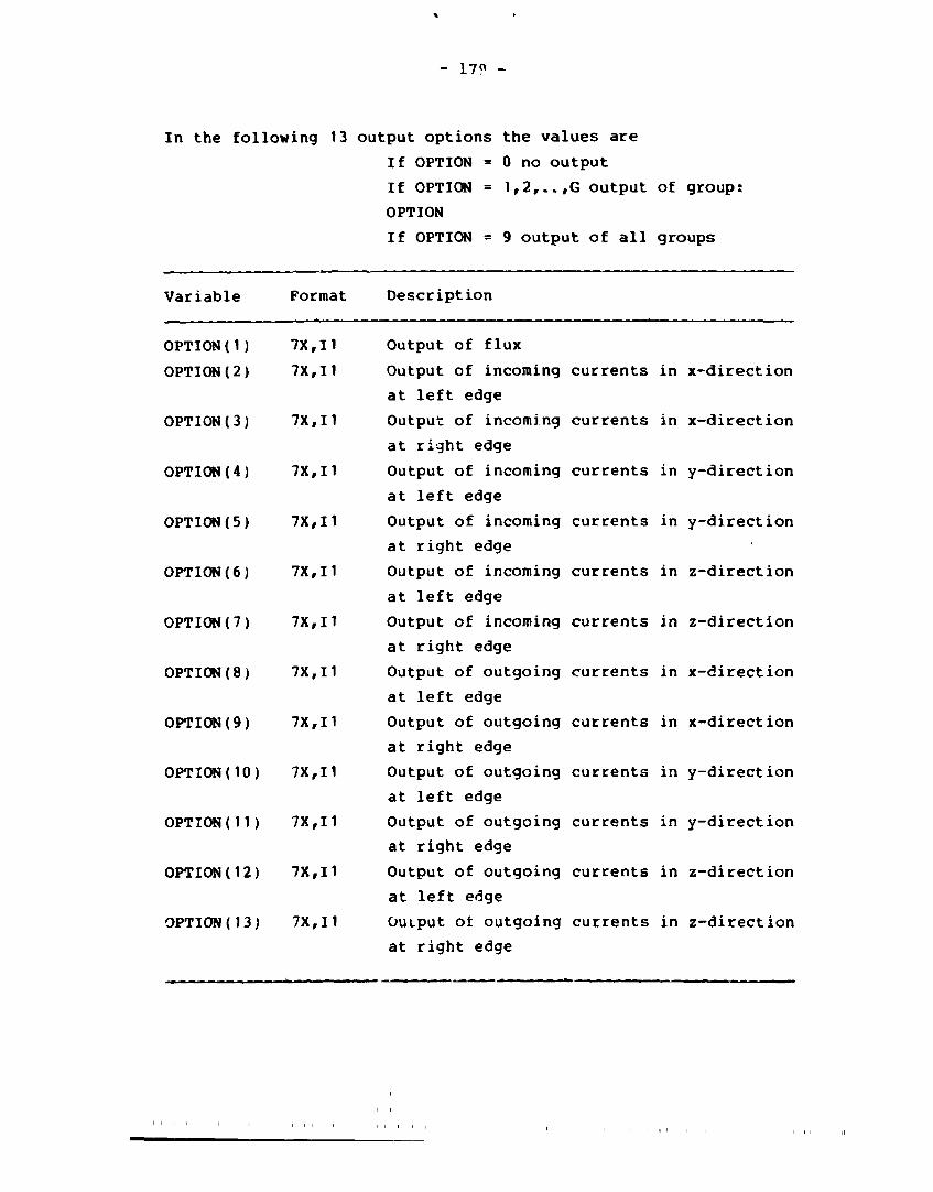
- 17? -

In the following 13 output options the values are

If OPTION = 0 no output

If OPTION = 1,2,..,G output of group:

OPTION

If OPTION = 9 output of all groups


OPTION(I) 7X,I1 Output of flux

OPTION(2) 7X,I1 Output of incoming currents in x-direction

at left edge

OPTION(3) 7X,I1 Output of incoming currents in x-direction

at right edge

OPTION(4) 7X,I1 Output of incoming currents in y-direction

at left edge

OPTION(5) 7X,I1 Output of incoming currents in y-direction

at right edge

OPTION(6) 7X,I1 Output of incoming currents in z-direction

at left edge

0PTI0N(7) 7X,I1 Output of incoming currents in z-direction

at right edge

OPTION(8) 7X,I1 Output of outgoing currents in x-direction

at left edge

OPTION(9) 7X,I1 Output of outgoing currents in x-direction

at right edge

OPTION(10) 7X,I1 Output of outgoing currents in y-direction

at left edge

OPTION(H) 7X,I1 Output of outgoing currents in y-direction

at right edge

OPTION(12) 7X,I1 Output of outgoing currents in z-direction

at left edge

OPTION(13) 7X,I1 Output of outgoing currents in z-direction

at right edge

- 180 -

Variable Factor Description

OPTION(M) 7X,I1

OPTION(15) 7X,T1

OPTION(16) 7XrI1

OPTION(17) 7X,I1

OPTION(18) 7X,I1

OPTION(19) 7X,I1

OPTION(20) 7X,I1

OPTION(21) 7X,I1

OUTPUT(22) 7X,I1

OPTION(K+21) 7X,I1

OPTION(62) 7X,I1

OPTION(63) 7X,I1

OPTION(64) 7X,I1

OPTION(65) 7X,I1

OPTION(66) 7X,I3

OPTION(OPTION(65)+65)

7X,I3

If OPTION(14)=1 output of fuel types

If OPTION(15) = 1 output of eigenvalue for

each outer iteration

If OPTION(16) « 1 output of multiplication

factor for each inner iteration

If OPTION(17) * 1 output of start values

(tho&e defined in option 1 to 14 and

21 to 61)

If 0PTION(18) > 0 number of outer itera

tion between output of option 1-14, 21-60

If OPTION(19) » 1 output after each inner

iteration

If OPTION(20) - 1 output at end If OPTION(21) - 1 output of power

If OPTION(22) = 1 output of layer 1

(option 1-14 and 21)

If OPTION(K+21) * 1 output of layer K

(option 1-14 and 21)

If OPTION(62) * 1 output to plotfile of

horizontal view

If OPTION(63) - 1 output to plotfile

of horizontal view at x - 0. The output

variable are those defined in option 1-

14, 21-41

If 0PTILN(64) » 1 output to plotfile of

horizontal view at x * y

Number of channels in which a vertical

view is written to plotfile 13. The out

put variables are those defined in option

1-14, 21

Channel number for output to plotfile.

If the nodes in the bottom is (1,j,i)

the channel number is

i-1 I [jMAX(n)-JMIN(n)+1]+j

n-1

- 181 -


OPTIurt(80) 7X,I3 If OPTION(80) = 0 no reference solution

If OPTION(80) = 1 a reference solution is

read and can be compared with the cal

culated one if power output is defined

(OPTION(21))

The following cards are only read if option(80) = 1

EO 7X,F10.6 The eigenvalue of the reference

solution

80X

REF(JMIN(1 ), 1 ) 710.3 The normalizewd power distribution of

REF(JMIN(1) + 1,1 ) the reference solution. The normalization

is only over powers > 0. For

REF(JMAX(1 ),1 ) three-dimensional problems it is the

REF(JMIN(2),2) assembly power distribution.

Only one row on each card

REF(JMAX(2),2)

REF(JMAX(I)rI)

The following cards are read if NPART > 0 and they are repeated

NPART times

NFACTX 7X,I3 Refinement factor in the x-direction

NPACTY 7X,I3 Refinement factor in the y-direction

N^'ACTZ 7X,I3 Refinement factor in the z-direction

- 182 -

Input description for the dynamic part of NEM

First, the kind of transient has to be incorporated in the

program in form of a subroutine PARAM which gives the cross

section variation as i. action of time

The subroutine has to be declared:

SUBRUTINE PARAM(I,J,K,G,NNODE,NODE,D,SIGA,USIG,SIGG)

INTEGER G,I,J,K,NNODE,NODC(K,J,I)

REAL D(G,NNODE),SIGA(G,NNODE),USIG(G,NNODE),SIGG(G,G,

NN0DE),C0M(8)

COMMON /DYNCOM/COM

The parameters are

G Number of energy groups

I Maximum number of nodes in x-direction

J Maximum number of nodes in y-direction

K Maximum number of nodes in z-direction

NNODJS Number of different fuel types

NODE Fuel type in each node

D Diffusion constants for each group a-.d fuel type

SIGA Absorption cross section for each group and fuel

type

USIG v * If foe each group &nd fuel type

SIGG Scattering cross section for each fuel type

C0M(1) Time step just now

C0M(2) Current time

COM(3)-COM<8) Not used

The subroutine can be bound on the main program

First, a steady-state run has to be made with NSTART

corresponding to a dump for restart.

= 1

The files in use are the same as for the steady-state program.

Input from file 5.

- 183 -


^ _ _ j .

TEXT

NSTART

L

V(1)

V(G)

BETA(1)

BETA(L)

DECAY(1)

DECAY(L)

DT

DTMIN

TEND

MAXIN

ITGOOD

NODE

DF

POWER

13A6 The heading text

7X,I3 NSTART = 2, restart from dump

7xfI_ Number of precursor families 1 < L < 6

feOX

80X

7E10.3 The neutron velocities in each group

80X

7E10.3

80X

7E10.3

The S-value for each precursor family

The decay constants for each

precursor family

7X,E10.3 Guess on the first time step

7X,E10.3 Mininum allowed time step

7X,E10.3 The end time for the integration

5X,I5 The maximum number of inner

iterations, before halving the time step

7X,I3 Minimum number of time steps before time

step increase is attempted.

7X,I3 If MODE = 2 the convergence criterion

for convergence in inner iterations has

to be kept for the fluxes in all nodes

and energy groups.

If MODE • 2 the convergence criterion is

used on a weighted sum of fluxes

7X,E10.3 Convergence criterion for the flux in

the inner iterations

7X,E10.3 The nominal reactor power

- 184 -

In the following 13 output options the values are

if OPTION = 0 no output

if OPTION = 1,2, ,.,G output of group: OPTION

output of all groups if OPTION « 9


OPTION(I)

OPTION(2)

OPTION (3)

OPTION(4)

OPTION(5)

OPTION(6)

OPTION(7)

OPTION(8)

OPTION (9)

OPTION(10)

OP'HON(11)

OPTION(12)

OPTION(13)

7X,I

7X,I

7X,I

7X,I

7X,I

7X,I

7X,I

7XrI

7X,I

7X,I

7X,I

7X,I

7X,I

Output of flux

Output of incoming currents in redirec

tion at left edge

Output of incoming currents in x-direc-

tion at right edge

Output of incoming currents in y-direc-

tion at left edge

Output of incoming currents in y-direc-

tion at right edge

Output of incoming currents in z-direc-

tion at left edge

Output of incoming currents in z-direc-

tion at right edge

Output of outgoing currents in x-direc-

tion at left edge

Output of outgoing currents in x-direc-

tion at right edge

Output of outgoing currents in y-direc-

tion at left edge

Output of outgoing currents in y-direc-

tion at right edge

Output of outgoing currents in z-direc-

tion at left edge

Output of outgoing currents in z-direc-

tion at right edge

- 185 -


OPTION(14)

OPTION(15)

OPTION(16)

OPTION(17) 7X,I1

OPTION(18) 6X,I5

OPTION(19)

OPTION(20)

OPTION(21)

OPTION(22)

7XrI1 If OPTION(14)=1 output of fuel types

7xfI1 Not used

7X,I1 If OPTION(16) = 1 output of step length

nominal reactor power etc. for each

time step

If OPTION(17) = 1 output of start values

(those defined in option 1 to 14 and

21 to 61)

If OPTION > 0: Option(18)*DT time between

output of distributions (chosen by

OPTION(I) - OPTION(14) and OPTION(21)-

OPTI0N(61)). If OPTION(18) = 0 no output

7XrI1 If OPTION(19) = 1 output after each

inner iteration

7X,I1 If OPTI0N(20) = 1 output at end

7X,I1 If OPTI0N(21) = 1 output of power

7X,I1 If OPTION(22) = 1 output of layer 1

(OPTION 1-14 and 21)

OPTION(K+21) 7X,I1

OPTION(62) 7X,I1

OPTION(63) 7X,I1

OPTION(64) 7X,I1

OPTION(65) 7X,I1

If OPTI0N(K+21) output of layer K

(OPTION 1-14 and 21)

If OPTION(62) = 1 output to plotfile of

horizontal view

If OPTION(63) = 1 output to plotfile 11

of horizontal view at x = Q. The out

put-variables are those defined in

OPTION 1-14 and 21-41

If OPTION(64) = 1 output to plotfile 12

of horizontal view at x = y

Number of channels in which a vertical

view is written to plotfile 13. The

output variables are those defined in

OPTION 1-1 and 21.

- 186 -


OPTION(66) 7X,I3 Channel number for output to plotfile.

If the nodes in the botton is (1,jri)

OPTION(OPTION(65)+65) the channel number is

7X,I3 i-1

I (JMAX(n) - JMIN(n)+1) + j n=1

OPTION(80) 7X,I3 Not used.

- 187 -

APPENDIX E

E.l Input example for steady-state calculation.

7BEGIN JOB LMWLWR;CLASS=1;CHARGE=3020501

?MAXPROCTIME=3^0;MAXIOTIME=300;MAXLINES=2000

?DESTNAME=RTA

?RUN 0BJECT/NEM/LMWLWR3D/A

7FILE FILE5(KINr-=fiEADEP)

7FILE FILE6(KIND=DISK,MAXRECSIZE=22,BL0CKSIZEr330)

7FILE FILE6(»,TITLEsLMWLWR/0UTPUT,PROTECTIONsSAVE)

7FILE FILE10(TITLE=DUMP/LMWLWR3D)

7FILE FILE11(TITLE=PLOT/HORIZ0NTAL/I0/LMWLWR3D)

7FILE FILE12(TITLE=PLOT/HORIZONTAL/IJ/LMWLWR3D)

7FILE FILE13(TITLE=PLOT/VERTICAL/LMWLWR3D)

7DATA

1 8 8 -

LKW LWR TRANSIENT BENCHMARK. 1/8 CORE. 200 NODES. 20 CM NODES

NSTART 1

IMAX *

JMAX 6

KMAX 10

N 200

GROUPS 2

NNODE 4

NAPP 4

TDUMP 2 . 6 0 0 E + 0 2

ISYM 6

NSYM 3

IMTN

1 1 1 1 1 1

IMAX

1 2 3 4 5 5

JMIN

1 2 3 4 5

JMAX

6 6 6 6 6

NODE

4 4 4 4 4 4

4 4 4 4 4

4 4 4 4

4 4 4

4 4

1 1 1 1 3 4

1 1 1 3 4

1 1 3 4

3 3 4

4 4

1 1 1 1 3 4

1 1 1 3 4

1 1 3 4

3 3 4

4 4

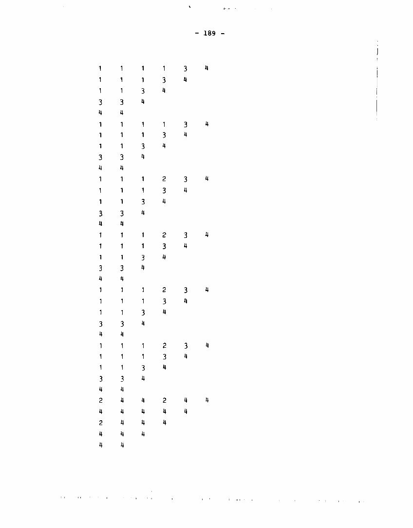
- 189 -

1 1 1 1 3 ^

1 1 1 3 4

1 1 3 4

3 3 4

4 4

1 1 1 1 3 4

1 1 1 3 4

1 1 3 4

3 3 4

4 4

1 1 1 2 3 4

1 1 1 3 4

1 1 3 4

3 3 4

4 4

1 1 1 2 3 4

1 1 1 3 4

1 1 3 4

3 3 4 4 4

1 1 1 2 3 4

1 1 1 3 4

1 1 3 4

3 3 4

4 4

1 1 1 2 3 4

1 1 1 3 4

1 1 3 1

3 3 4

4 4

2 4 4 2 4 4

4 4 4 4 4

2 4 4 4

4 4 4

4 4

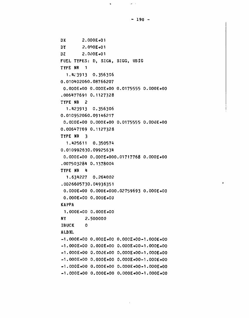
- 190 -

DX 2.000E+01

DY 2.000E+01

DZ 2.000E+01

FUEL TYPES: D, SIGA, SIGG, USIG

TYPE NR 1

1 .Ui 3913 0 . 3 5 6 3 0 6

0 . 0 1 0 4 0 2 0 6 0 . 0 8 7 6 6 2 0 7

0 .000E+00 0 .000E+00 0 . 0 1 7 5 5 5 5 0.000E+00

.006477691 0 . 1 1 2 7 3 2 8

TYPE NR 2

1.423913 0.356306

0.010952060.09146217

O.OCOE+00 O.OOOE+00 0 . 0 1 7 5 5 5 5 O.OOOE+00

0 . 0 0 6 4 7 7 6 9 0 . 1 1 2 7 3 2 8

TYPE NR 3

1.425611 0.350574

0.010992630.09925634

0.000E+00 0 . 0 0 0 E + 0 0 0 . 0 1 7 1 7 7 6 8 O.OOOE+00

.007503284 0 . 1 3 7 8 0 0 4

TYPE NR 4

1.634227 0.264002

.0026605730.04936351

0.00OE+00 0 . 0 0 0 E + 0 0 0 . 0 2 7 5 9 6 9 3 0 .000E+00

0 .000E+00 O.OOOE+00

KAPPA

1.000E+00 0.000E+00

NY 2 . 5 0 0 0 0 0

IBUCK 0

ALBXL

-1 .000E+00 0.000E+00 0.000E+00-1.OOOE+00

-1 .000E+00 0.000E+00 0.O00E+0O-1.OOOE+00

-1 .000E+00 0.000E+00 0.000E+00-1.OOOE+00

-1 .000E+00 0.000E+00 0 .000E+00-1 .000E+00

- 1 . 0 0 0 E + 0 0 O.OOOE+00 0.000E+OO-1.OOOE+00

-1 .000E+00 O.OOOE+00 0 .000E+00-1 .000E+00

- 1 9 1 -

ALBXR

- 1 . O O O E + 0 0 O.OOOE+OO O . O O O E + 0 0 - 1 . O O O E + 0 0

- 1 . O O O E + 0 0 O.OOOE+OO O.OOOE+OO-1.COOE+OO

- 1 . 0 O 0 E + 0 O O.OOOE+OO O.OOOE+OO-1.OOOE+OO

- 1 . O O O E + 0 0 O.OOOE+OO O.OOOE+OO-1.OOOE+OO

-1 .OOOE+OO O.OOOE+OO O.OOOE+OO-1.OOOE+OO

-1.OOOE+OO O.OOOE+OO 0.OOOE+OO-1.OOOE+OO

ALBYL

- 1 . O O O E + 0 0 O.OOOE+00 0 . O ' O E + 0 0 - 1 . O O O E + O O

- 1 . O O O E + 0 0 O.OOOE+OO O.OOOE+00-1.OOOE+OO

- 1 . 0 0 0 É + 0 0 O.OOOE+00 O . O O O E + 0 0 - 1 . O O O E + 0 0

-1 .OOOE+OO O.OOOE+OO O.OOOE+00-1.OOOE+OO

- 1 . O O O E + 0 0 O.OOOE+00 O . O O O E + 0 0 - 1 . O O O E + 0 0

ALBYR

- 1 . O O O E + 0 0 O.OOOE+OO O.OOOE+00-1.OOOE+OO

- 1 . O O O E + 0 0 O.OOOE+00 O . O O O E + 0 0 - 1 . O O O E + 0 0

- 1 . O O O E + 0 0 O.OOOE+OO 0 .OOOE+00-1 .OOOF+OO

-1.OOOE+00 O.OOOE+00 O.OOOE+00-1.OOOE+00

- 1 . O O O E + 0 0 O.OOOE+OO 0 .OOOE+00-1 .OOOE+OO

ALBZL

- 1 . O O O E + 0 0 O.OOOE+00 0 . O O O E + 0 0 - 1 . O O O E + 0 0

ALBZR

-1.OOOE+OO O.OOOE+OO 0 . O O O E + 0 0 - 1 . O O O E + 0 0

NPART O

MAXIN 17

MAXOUT TOO

LEAK

UPDATE

MODE

GAMMA

EIGV

DL

DF

FI

CIM XL

CINXR

CINYL

CINYR

CINZL

2

3 0

O.OOOE+OO

1.OOOE+00

1.000E-06

1.000E-OH

0

0

0

0

0

0

- 192 -

CINZR

CXL

CXR

CYL

CYR

CZL

CZR

NODE

EIGV

FACT

START

OUTER

INNER

END

POWER

Kl PLOT

K2PL0T

K3PLOT

K4PL0T

K5PL0T

K6PLOT

K7PL0T

K8PL0T

K9PLOT

0

0

0

0

0

0

0

0

1

0

0

0

0

1

1

0

0

0

0

0

0

0

0

0

K10PLOTO

RADPLOTO

IOPLOT

IJPLOT

ANTKAN

REF

0

0

0

0

?END JOB

\

- 193 -

E.2 Input example f o r dynamic c a l c u l a t i o n .

?BEGIN JOB LMWLWR/DYN;CLAS3=4;CHARGE=30£05O1

?h.\XPROCTIME=Un00;MAXIOTIME=60;MAXLINES=50O0

?DESTNAME=RTA

?RUN 0BJECT/NEM/LMWLWR3D/A

?FILE FILE5(KIND=READER)

?FiLE FILE6(KIND=DISK,MAXRECSIZE=22,BLOCKSIZE=330)

?FILE FILE6(»,TITLE=LMWLWR/0UTPUT/DYN,PR0TECTI0N=SAVE)

?FILE FILE7(TITLE=FILE7/LMWLWR3D,PROTECTION=SAVE,NEWFILE=TRUE)

?FILE FILE 10(TITLE=DUMP/LMWLWR3D)

?FILE FILE11(TITLE=PLOT/HORIZONTAL/I0/LMWLWR3D)

?FILE FILE 12(TITLE=PL0T/H0RIZ0NTAL/IJ/LMWLWR3D)

?FILE FILE13(TITLE=PLOT/VERTICAL/LMWLWR3D)

?DATA

- 194 -

LMULWR 3D REACTOR KINETICS BENCHMARK. DYNAMIC.

NSTART 2

L 6

DYNAMIC INPUT

NEUTRON VELOCITIES

1.250E+07 2.500E+05

BETAS

2 .470E-04 0 .0013845 1 .222E-03 0 .0026455 8 .320E-04 1.690E-04

DECAY CONSTANTS

1.270E-02 3-17CE-02 1.150E-01 3 .110E-01 1.400E+00 3.870E+00

DT 2 .500E-01

DTMIN 1.000E-C3

6.000E+01

20

10

2

1.000E-02

1.500E+02

TEND

MAXIN

ITDOUB

MODE

DF

POWER

FI C IN XL

CINXR

CINYL

CINYR

CINZL

CINZR

CXL

CXR CYL CYR

CZL CZR NODE

EIGV

FACT

START

OUTER

INNER

END POWER

i

0

0 0 0

0 0

0

0 0 0 0

0 0 0 1

1 1

0 1 1

40

Kl PLOT 0

K2PL0T 0

K3PLOT 0

KIP'OT 0

K5PLOT 0

K6PLOT 0

K7PLOT 0

K8PLOT 0

K9PLOT 0

K10PLOTO

RADPLOTO

IOPLOT O

Uf-LOT 0

ANTKAN 0

REF 0

?EHD JOB

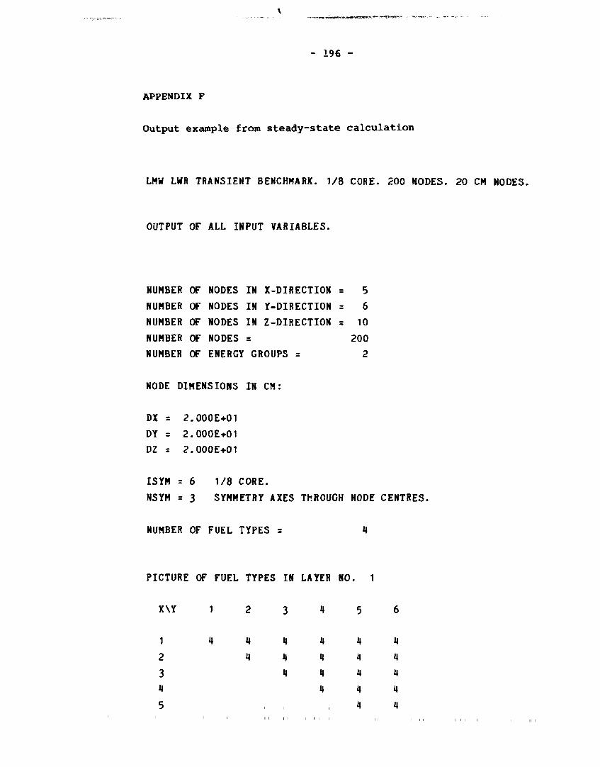
- 196 -

APPENDIX F

Output example from steady-state calculation

LMW LWR TRANSIENT BENCHMARK. 1/8 CORE. 200 NODES. 20 CM NODES.

OUTPUT OF ALL INPUT VARIABLES.

NUMBER OF NODES IN X-DIRECTION = 5

NUMBER OF NODES IN Y-DIRECTION = 6

NUMBER OF NODES IN Z-DIRECTION = 10

NUMBER OF NODES = 200

NUMBER OF ENERGY GROUPS = 2

NODE DIMENSIONS IN CM:

DX - 2.000E+01

DY = 2.000E+01

DZ = 2.000E+01

ISYM = 6 1/8 CORE.

NSYM = 3 SYMMETRY AXES THROUGH NODE CENTRES.

NUMBER OF FUEL TYPES = 4

PICTURE OF FUEL TYPES IN LAYER NO. 1

X\Y 1 2 3 t 5 6

1 4 4 4 4 4 4

2 4 4 4 4 H

3 4 4 4 4

4 4 4 4

5 4 4

- 197 -

PICTURE OF FUEL TYPES IN LAYF.t NO.

X\Y 1 2 3 4 5

1

2

3

4

5

1

1

1

1

1

1

1

1

3

3 3 3 3 4

4

4

4

4

4

PICTURE OF FUEL TYPES IN LAYER NO.

X\Y 1 2 3 4

1

2

3

4

5

1

1

1

1

1

1

1

1

3

3

3 3 3

4

4

4

4


X\Y

1

2

3

4

5

1

1

1

1

1

1

1

1

3

3 3 3 3 4

4

4

4

4

4

- 198 -


X\Y 1 2 3 4 5

1

2

3

4

5

1

1

1

1

1

1

1

1

3

3

3

3

3

4

4

4

4


X\Y 1 2 3 4

1

2

3

4

5

1

1

1

1

1

2

1

1

3

3

3

3

3 4

4

4

4

4

4


X\Y 1 2 3 4 5

1

2

3

4

5

1

1

1

1 1

2

1 1

3

3

3 3 3 4

4

4

4

4

4

- w " T*- t*--«.r«j«^TJ«l«a}Mj^^^'<!»^«Ha«WBr^^-—w^-./-

- 199 -


X\Y 1 2 3 4 5

1

2

3

4

5

1

1

1

1

1

2

1

1

3

3 3 3 3

4

4

4

4

4

4

PICiURE OF FUEL TYPES IN LAYER NO.

X\Y 1 2 3 4

1

2

3

4

5

1

1

1

1

1

2

1

1

3

3 3 3 3

4

4

4

4

4

4


X\Y 1 2 3 4 5 6

1 2 4 4 2 4 4

2 4 4 4 4 4

3 2 4 4 4

4 4 4 4

5 4 4

*

- 200 -

PARAMETERS FOR FUEL TYPE NO. 1

DIFFUSION COEFFICIENTS IN CM:

1.H24E+00 3.563E-01

ABSORPTION CROSS SECTIONS IN CM**(-1):

1.0UOE-02 8.766E-02

SCATTERING CROSS SECTIONS IN CM»«(-1):

0. 0. 1.756E-02 0.

NY*FISSION CROSS SECTIONS IN CM**(-1):

6.478E-03 1.127E-01



1.424E+00 3.563E-01

ABSORPTION CROSS SECTIONS IN CM*»(-1):

1.095E-02 9.1M6E-02

SCATTERING CROSS SECTIONS IN CM«»(-1):

0. 0. 1.756E-02 0.

NY»FISSION CROSS SECTIONS IN CM«»(-1):

6.478E-03 1.127E-01

- 201 -



1.M26E+00 3.506E-O1

ABSORPTION CROSS SECTIONS IN CM**(-1):

1.O99E-02 9.926E-02

SCATTERING CROSS SECTIONS IN CM*«(-1):

0. 0. 1.718E-02 0

NY*FISSION CROSS SECTIONS IN CM**(-1):

7.503E-03 1.378E-01

PARAMETERS FOR FUEL TYPE NO. M


1.634E+00 2 .640E-01

ABSORPTION CROSS SECTIONS IN CM*»(-1):

2 .661E-03 4 .936E-02

SCATTERING CROSS SECTIONS IN CM**(-1):

0 . 0 . 2 .760E-02 0

NY«FISSION CROSS SECTIONS IN CM»«(-1):

0 . 0 .

KHI:

1.000E+00 0 .

- 202 -

NY = 2.500E+00

IBUCK:

ALBEDOS:

X-DIRECTION - LEFT EDGE:

1.OOOE+00

1.OOOE+00

1.OOOE+00

1.OOOE+00

1.OOOE+00

1.OOOE+00

0.

0.

0.

0.

0.

0.

0.

0.

0.

0.

0.

0.

-1.OOOE+OO

-1.OOOE+00

-1.OOOE+00

-1.000E.30

-1.OOOt,00

-1.OOOE+00

X-DIRECTION - RIGHT EDGE:

1.OOOE+OO

1.0001+00

1.OOOE+OO

1.OOOE+00

1.OOOE+00

1.OOOE+OO

0.

0.

0.

0.

0.

0.

0.

0.

0.

0.

0.

0.

-1.OOOE+OO

-1.OOOE+00

-1.OOOE+OO

-1.OOOE+00

-1.OOOE+00

-1.OOOE+00

- 203 -

Y-DIRECTION - LEFT EDGE:

1.000E+00

1.OOOE+00

1.OOOE+00

1.OOOE+00

1.OOOE+00

0 .

0 .

0 .

0 .

0 .

0 .

0 .

0 .

0 .

0 .

-1.OOOE+00

-1.OOOE+00

-1.OOOE+00

-1.OOOE+00

-1.OOOE+00

Y-DIRECTIOM - RiC.HT EDGE:

1 .OOOE+00

1.OOOE+00

1 . 0 0 0 E + 0 0

1 . 0 0 0 E + 0 0

1.OOOE+00

0 .

0 .

0 .

0 .

0 .

0 .

0 .

0 .

0.

0 .

-1.OOOE+00

-1.OOOE+00

-1.OOOE+00

-1.OOOE+00

-1.OOOE+00

Z-DIRECTION - LEFT EDGE:

-1.000E+00 0. -1.000E+00

Z-DIRECTION - RIGHT EDGE:

-1.OOOE+00 0. -1.000E+00

- 204 -

TIME LIMIT FOR DUMP = 2 . 6 0 0 E + 0 2 SECONDS

APPROXIMATION ORDER = «

NUMBER OF REFINEMENTS = 0

NUMBER OF INNER ITERATIONS = 17

NUMBER OF OUTER ITERATIONS = 100

LEAKAGE APPROXIMATION ORDER = 2

ITERATIONS BETWEEN UPDATING = 3

MODE = 0

GAMMA = 0 .

EIGENVALUE = 1 . 0 0 0 E + 0 0

DEVIATION ON EIGENVALUE = 1 . 0 0 0 E - 0 6

DEVIATION ON FLUX = 1.000E-OU

OUTPUT OPTIONS :

15 : OUTPUT OF EIGENVALUE FOR EACH OUTER ITERATION

20 : OUTPUT AT END

21 : OUTPUT OF POWER

- 205 -

LMW LWR TRANSIENT BENCHMARK. 1/8 CORE. 200 NODES. 20 CM NODES.

1

2

3

4

5

6

7

8

9

10

11

12

M

14

15

16

17

18

19

20

21

22

23

24

OUTER

OUTER

OUTER

OUTER

OUTER

OUTER

OUTER

OUTER

OUTER

OUTER

OUTER

OUTER

OUTER

OUTER

OUTER

OUTER

OUTER

OUTER

OUTER

OUTER

OUTER

OUTER

OUTER

OUTER

17

17

17

17

17

20

17

17

17

17 20

17

17

17

17

20

17

17

17

17 20

17

17

17

INNER

INNER

INNER

INNER

INNER

INNER

INNER

INNER

INNER

INNER

INNER

INNER

INNER

INNER

INNER

INNER

INNER

INNER

INNER

INNER

INNER

INNER

INNER

INNER

ITERATIONS

ITERATIONS

ITERATIONS

ITERATIONS

ITERATIONS

ITERATIONS

ITERATIONS

ITERATIONS

ITERATIONS

ITERATIONS

ITERATIONS

ITERATIONS

ITERATIONS

ITERATIONS

ITERATIONS

ITERATIONS

ITERATIONS

ITERATIONS

ITERATIONS

ITERATIONS

ITERATIONS

ITERATIONS

ITERATIONS

ITERATIONS

EIGENVALUE

EIGENVALUE

EIGENVALUE

EIGENVALUE

EIGENVALUE

EIGENVALUE

EIGENVALUE

EIGENVALUE

EIGENVALUE

EIGENVALUE

EIGENVALUE

EIGENVALUE

EIGENVALUE

EIGENVALUE

EIGENVALUE

EIGENVALUE

EIGENVALUE

EIGENVALUE

EIGENVALUE

EIGENVALUE

EIGENVALUE

EIGENVALUE

EIGENVALUE

EIGENVALUE

0.9824223

0.9882730

0.9934466

0.9962038

0.9995961

0.9988922

0.9990594

0.9992524

0.9993698

0.9995440

0.9995017

0.9995092

0.9995192

0.9995260

0.9995371

0.9995337

0.9995341

0.9995347

0.9995351

0.9995990

0.9995461

0.9995373

0.9995360

0.9995358

OUTER ITERATION NUMBER = 24 INNER ITERATION NUMBER = 17

- 206 -

PICTURE OF FOWER IN HORIZONTAL LAYER.

X\Y 1 2 3 4 5 6

1 1.560 1.176 1.283 0.982 0.642 0.000

2 1.417 1.244 0.964 0.626 0.000

3 1.126 0.873 0.554 0.000

4 0-763 0.380 0.000

5 0.000 0.000

PICTURE OF POWER IN VERTICAL DIRECTION.

0

9

8

7 6

5 4

3 2

1

0.015

0.451 0.884

1.222

1.418

1.446

1.278

0.934

0.469

0.000

AFTER 24 OUTER ITERATIONS THE PROGRAM IS TERMINATED WITH A

DUMP ON FIL

Sales distributors: G.E.C. Gad Strøget Vimmelskaftet 32 DK-1161 Copenhagen K, Denmark

Available on exchange from: Risø Library, Risø National Laboratory, ISBN 87-550-1169-1 P.O.Box 49, DK-4000 Roskilde, Denmark ISSN 0106-2840

three-dimensional static and dynamic reactor calculations

Documents