three-dimensional numerical simulation model of biogas...
TRANSCRIPT

2
An ASABE Meeting Presentation
Paper Number: 064060
Three-Dimensional Numerical Simulation Model of Biogas Production for Anaerobic Digesters
Binxin Wu, Research Associate Dept. of Mechanical and Manufacturing Engineering, University of Manitoba, Winnipeg, MB, R3T 5V6, Canada. [email protected]
Eric L. Bibeau, Assistant Professor Dept. of Mechanical and Manufacturing Engineering, University of Manitoba, Winnipeg, MB,
R3T 5V6, Canada.
Kifle G. Gebremedhin, Professor Dept. of Biological and Environmental Engineering, Cornell University, Ithaca, NY, 14853, USA
Written for presentation at the 2006 ASABE Annual International Meeting
Sponsored by ASABE Oregon Convention Center
Portland, Oregon 9 - 12 July 2006
Abstract. A review of the modeling of biogas production from anaerobic digesters is first conducted. A three-dimensional numerical simulation model that predicts biogas production from a plug-flow anaerobic digester is developed. The model is based on the principles of continuity, energy, and species transport. A first-order kinetic model is used to predict the chemical reactions and BOD (Biological Oxygen Demand) in the digestion process. A user-defined function for computing the chemical source terms of the finite rate model is developed. The anaerobic digestion and simulation are conducted using Fluent 6.1 to predict the temperature profile and concentration distribution in the digester. Model predictions are validated against experimentally measured biogas production data obtained from the literature. The results agree within 5%.
Keywords. Numerical Simulation, Anaerobic Digester, Chemical Reaction, Biogas Production.
3
Introduction Anaerobic digestion of cow or swine manure is a source of renewable energy. The anaerobic
digestion process reduces the solid content of the influent and produces less offensive odors. The
process involves transformation of the organic compounds, by microorganisms, into microbial
biomass and other simpler compounds, eventually releasing water, carbon dioxide, and methane.
Biogas production using anaerobic digesters has been experimentally and theoretically studied
since the 1960s (Buswell and Mueller, 1962). Biogas production models have evolved from
simple models (Jewell, 1978; Chen and Hashimoto, 1978; Safely and Westerman, 1992, 1994;
Toprak, 1995; Hobbs et al., 1999; Andara and Esteban, 1999; Masse and Droste, 2000) to a
complex model (Scott and Minott, 2002). In the simple models, if any of the assumed
parameters such as digester volume or slurry temperature is changed, the models become no
more valid. The complex model (Scott and Minott, 2002) contains more input parameters
compared to the simple models. The inputs include: hydraulic retention time, initial volatile
solids concentration, bacterial growth rate at fixed digester temperature, digester volume, and
daily flow rate of manure influent. However, these models are one-dimensional (the spatial
parameters are not taken into consideration), and it is known that biogas production is sensitive
to digester temperature, pH of the liquid manure, and non-uniformity of flow pattern of liquid
manure inside the digester. In previous studies (Hashimoto et al., 1981; Safely and Westerman,
1992, 1994; Scott and Minott, 2002), these parameters were assumed to be constants. To our
knowledge, no three-dimensional numerical simulation model that predicts biogas production
from local flow conditions for mixing-flow and plug-flow type digesters has been reported.
Objectives:
The objectives of this study are to:
(1) conduct a comprehensive literature review on modeling biogas production from anaerobic
digestion,
(1) develop a general and fundamentally-based three-dimensional numerical model that predicts
biogas production from plug-flow type digesters, and
4
(2) validate the model predictions against experimental data obtained from the literature.
Literature Review Buswell and Mueller (1962) developed a model that predicts methane production from chemical
composition of degradable waste. The model is expressed as
422 )482
()482
()24
( CHban
COban
OHba
nOHC ban −+++−⇔−−+ (1)
where, ban OHC is organic matter, OH2 is water, 2CO is carbon dioxide, 4CH is methane, a, b,
and n are dimensionless coefficients.
Jewell (1978) developed an empirical model for biogas production for a plug-flow digester and is
expressed as
HRTSSBG bbmethane /)(5.0 10 −= (2)
where, 0bS is influent biodegradable volatile solides (BVS) concentration (g/L), 1bS is effluent
BVS concentration (g/L), HRT is hydraulic retention time (days), and methaneBG is the volumetric
methane production rate: volume of gas produced per digester volume per day (L/ (L*day).
Chen and Hashimoto (1978) developed a model that predicts methane production rate and is
expressed as
0 0*
(1 )* 1v
m
B S K
HRT HRT Kγ
µ= −
− + (3)
where, vγ is methane production rate (L of 4CH per L digester volume per day), 0B is ultimate
methane yield (L 4CH /g VS added), 0S is influent volatile solid concentration (g/L), K is kinetic
parameter (dimensionless), and mµ is maximum specific growth rate ( 1−day ). The K parameter
was empirically determined from
5
)051.0( 00206.06.0 SeK ⋅+= (4)
The mµ value was calculated from (Hashimoto et al., 1981)
0.013* 0.129m Tµ = − (5)
where, T is digester temperature ( C0 ).
Bryant (1979) studied microbial methane production. He investigated the relationships of three
general metabolic groups of bacteria or stages of fermentation involved in methane fermentation.
The three metabolic groups of bacteria include: first-stage-fermentative bacteria, second-stage-
2H -producing acetogenic bacteria, and stoichiometry and kinetics of fermentation.
Hill (1982a, 1982b, and 1982c) performed computer analysis of microbial kinetics of methane
fermentation to show: (a) maximum volumetric methane production, and (b) maximum total
daily methane production to design the continuous flow anaerobic digester. He analyzed methane
fermentation kinetics to produce a set of optimized design criteria for steady-state digestion, and
developed a dynamic computer model to predict digester operating conditions (i.e., retention
time, loading rate, and temperature) for four major animal types (dairy, poultry, swine, and beef).
Hashimoto (1983) studied the effects of temperature (35 C0 and 55 C0 ), influent volatile solid
concentration and hydraulic retention time on methane production from swine manure.
Hashimoto (1984) experimentally determined the K parameter specific for swine manure. Later,
Hashimoto et al. (1994) discussed about commercializing the technology of methane production
from animal waste, and described the design and construction of a centralized anaerobic
digestion facility that converts dairy manure into electrical energy and fertilizer.
6
Fischer et al. (1984) operated an anaerobic digester using swine manure at high influent volatile
solids concentration, and evaluated the relationship between methane production per gram of
volatile solids added, and methane production per volume of digester, to hydraulic retention time
and influent volatile solids concentration.
Pavlostathis and Gossett (1986) examined the preliminary conversion step in detail by
considering mechanisms such as cell death/lysis, hydrolysis of particulate dead biomass,
acidogenesis, and methanogenesis. A kinetic model was proposed to describe digester
performance and predict effluent quality.
Costello et al. (1991a) developed a mathematical model of a high-rate anaerobic treatment
system by defining the biological make-up of an anaerobic ecosystem, the physico-chemical
system, and the reactor process. The overall reactor equations were described and included the
biological rate equations, and inhibitions and interactions within the anaerobic system. The
physico-chemical reaction system determined the ionic concentration of soluble components in
the reactor. Later, Costello et al. (1991b) validated their model against results obtained from two
laboratory-scale reactors and a pilot-scale.
Safely and Westerman (1992) determined the relationship between methane yield and digester
temperature in a low-temperature lagoon digester. The equation was expressed as
0.216 0.00934*B T= + (6)
where, B is methane production ( VSkgCHm /43 ), and T is digester temperature ( C0 ).
Safely and Westerman (1994) evaluated the performance of laboratory-scale anaerobic digesters
fed with dairy and swine manure at loading rates of 0.1 and 0.2 3/kgVS m day− over a
temperature range of 10 C0 -25 C0 , and reported the following equations to estimate methane
yield:
7
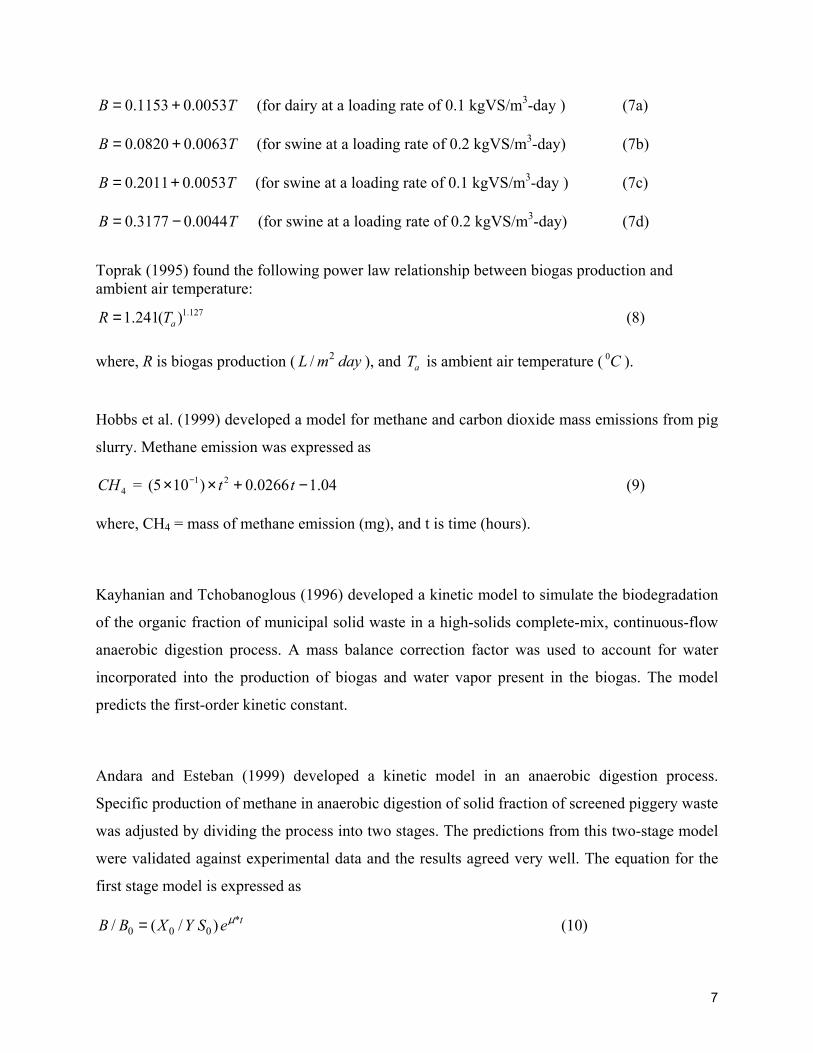
TB 0053.01153.0 += (for dairy at a loading rate of 0.1 kgVS/m3-day ) (7a)
TB 0063.00820.0 += (for swine at a loading rate of 0.2 kgVS/m3-day) (7b)
TB 0053.02011.0 += (for swine at a loading rate of 0.1 kgVS/m3-day ) (7c)
TB 0044.03177.0 −= (for swine at a loading rate of 0.2 kgVS/m3-day) (7d)
Toprak (1995) found the following power law relationship between biogas production and ambient air temperature:
127.1)(241.1 aTR = (8)
where, R is biogas production ( 2/L m day ), and aT is ambient air temperature ( C0 ).
Hobbs et al. (1999) developed a model for methane and carbon dioxide mass emissions from pig
slurry. Methane emission was expressed as
4CH = 04.10266.0)105( 21 −+×× − tt (9)
where, CH4 = mass of methane emission (mg), and t is time (hours).
Kayhanian and Tchobanoglous (1996) developed a kinetic model to simulate the biodegradation
of the organic fraction of municipal solid waste in a high-solids complete-mix, continuous-flow
anaerobic digestion process. A mass balance correction factor was used to account for water
incorporated into the production of biogas and water vapor present in the biogas. The model
predicts the first-order kinetic constant.
Andara and Esteban (1999) developed a kinetic model in an anaerobic digestion process.
Specific production of methane in anaerobic digestion of solid fraction of screened piggery waste
was adjusted by dividing the process into two stages. The predictions from this two-stage model
were validated against experimental data and the results agreed very well. The equation for the
first stage model is expressed as
*0 0 0/ ( / ) tB B X Y S eµ= (10)
8
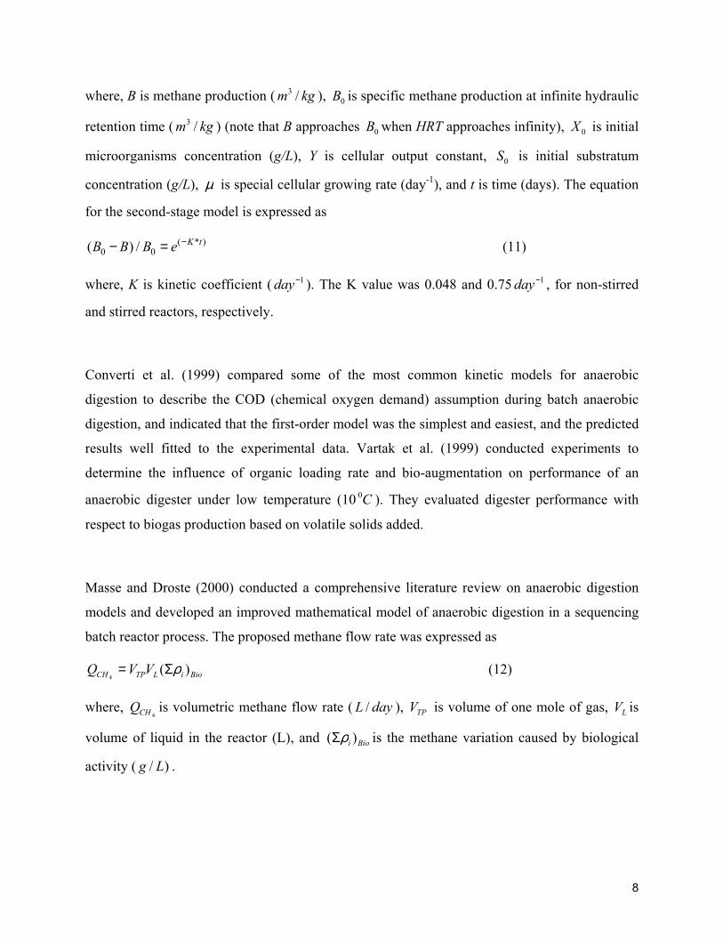
where, B is methane production ( kgm /3 ), 0B is specific methane production at infinite hydraulic
retention time ( kgm /3 ) (note that B approaches 0B when HRT approaches infinity), 0X is initial
microorganisms concentration (g/L), Y is cellular output constant, 0S is initial substratum
concentration (g/L), µ is special cellular growing rate (day-1), and t is time (days). The equation
for the second-stage model is expressed as
( * )0 0( ) / K tB B B e −− = (11)
where, K is kinetic coefficient ( 1−day ). The K value was 0.048 and 0.75 1−day , for non-stirred
and stirred reactors, respectively.
Converti et al. (1999) compared some of the most common kinetic models for anaerobic
digestion to describe the COD (chemical oxygen demand) assumption during batch anaerobic
digestion, and indicated that the first-order model was the simplest and easiest, and the predicted
results well fitted to the experimental data. Vartak et al. (1999) conducted experiments to
determine the influence of organic loading rate and bio-augmentation on performance of an
anaerobic digester under low temperature (10 C0 ). They evaluated digester performance with
respect to biogas production based on volatile solids added.
Masse and Droste (2000) conducted a comprehensive literature review on anaerobic digestion
models and developed an improved mathematical model of anaerobic digestion in a sequencing
batch reactor process. The proposed methane flow rate was expressed as
BioiLTPCH VVQ )(4
ρΣ= (12)
where, 4CHQ is volumetric methane flow rate ( /L day ), TPV is volume of one mole of gas, LV is
volume of liquid in the reactor (L), and Bioi )( ρΣ is the methane variation caused by biological
activity ( / )g L .
9
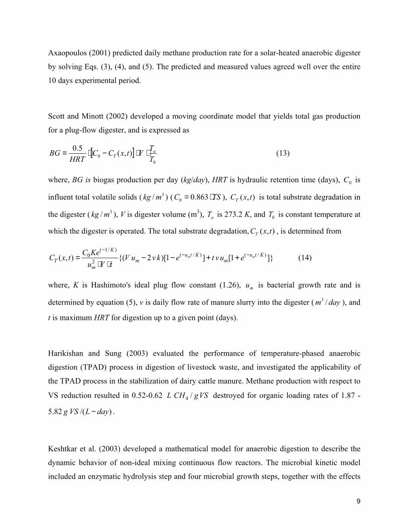
Axaopoulos (2001) predicted daily methane production rate for a solar-heated anaerobic digester
by solving Eqs. (3), (4), and (5). The predicted and measured values agreed well over the entire
10 days experimental period.
Scott and Minott (2002) developed a moving coordinate model that yields total gas production
for a plug-flow digester, and is expressed as
[ ]0
0 ),(5.0T
TVtxCC
HRTBG a
T ⋅⋅−⋅= (13)
where, BG is biogas production per day (kg/day), HRT is hydraulic retention time (days), 0C is
influent total volatile solids ( 3/ mkg ) ( TSC ⋅= 863.00 ), ),( txCT is total substrate degradation in
the digester ( 3/ mkg ), V is digester volume (m3), aT is 273.2 K, and 0T is constant temperature at
which the digester is operated. The total substrate degradation, ),( txCT , is determined from
( 1/ )( / ) ( / )0
2( , ) {( 2 )[1 ] [1 ]}m m
Ku t K u t K
T m mm
C KeC x t V u v k e t vu e
u V t
−− −= − − + +
⋅ ⋅ (14)
where, K is Hashimoto's ideal plug flow constant (1.26), mu is bacterial growth rate and is
determined by equation (5), v is daily flow rate of manure slurry into the digester ( daym /3 ), and
t is maximum HRT for digestion up to a given point (days).
Harikishan and Sung (2003) evaluated the performance of temperature-phased anaerobic
digestion (TPAD) process in digestion of livestock waste, and investigated the applicability of
the TPAD process in the stabilization of dairy cattle manure. Methane production with respect to
VS reduction resulted in 0.52-0.62 4 /L CH gVS destroyed for organic loading rates of 1.87 -
5.82 /( )g VS L day− .
Keshtkar et al. (2003) developed a mathematical model for anaerobic digestion to describe the
dynamic behavior of non-ideal mixing continuous flow reactors. The microbial kinetic model
included an enzymatic hydrolysis step and four microbial growth steps, together with the effects
10
of substrate inhibition, pH, and thermodynamics considerations. They concluded that methane
yield was strongly dependent on pH of the reactor and increased with greater HRTs.
McGrath and Mason (2004) developed a method for assessing biogas production based on visual
monitoring of biogas evolution events (size and frequency of gas occurring at the pond surface)
in an anaerobic waste stabilization pond, and then applied the method to anaerobic ponds that
treat farm dairy wastewater.
Karim et al. (2005) operated six laboratory-scale biogas mixed anaerobic digesters to study the
effect of biogas recycling rates and draft tube height on performance. They found higher
methane production rate in unmixed digesters, and increased biogas circulation rate reduced
methane production. No difference in methane production rate was observed with varying draft
tube height.
Blumensaat and Keller (2005) developed a process model to simulate the dynamic behavior of a
pilot-scale process for anaerobic two-stage digestion of sewage sludge. This process model
concept was a derivative of the International Water Association (IWA) Anaerobic Digestion
Model No.1 (ADM1) that had been developed by IWA task group. They did several
modifications to the original ADM1 model concept to allow an application for the pilot-scale
digestion process, and calibrated the model for a two-stage thermophilic/mesophilic process
configuration and municipal sewage sludge with typical characteristics as substrate input.
Model Development
Biogas production in an anaerobic digester is a chemical reaction process, which is governed by
mass and momentum conservations, turbulence, energy balance, species transport, and chemical
reactions. Because anaerobic digestion is dependent on process flow parameters and
temperatures, prediction of temperature and flow variables is an important component that
cannot often be neglected by assume bulk conditions prevail. This model was developed based
on the following assumptions:
11
• Heat flow and species transport through the digester are 3-D steady state.
• The model is limited to plug-flow anaerobic digesters where fluid flow is very low.
Thus, momentum and turbulence are considered to be negligible.
• The digester cover, walls, and floor are adiabatic.
• The liquid manure is assumed to be Newtonian fluid.
• The manure temperature is constant at 32 C0 before species reaction.
• Species reaction takes place only in one step, i.e., reactants can be directly converted into
products without intermediate products.
• The percentage remaining of reactant ( 6126 OHC ) is 80% after reaction.
• Biogas production doesn’t affect the transport of manure as it rises to the surface.
Mass Conservation Equation
The equation for conservation of mass, or continuity equation, is expressed as
( ) 0=∂
∂+∂∂
ii
uxt
ρρ (15)
where, t is time, ρ is density of mixture, and iu (and ju shown in the equation below) is
velocity in tense form.
Energy Equation
The energy equation is of the form (Patankar, 1980):
( ) ( )( ) ( ) hj
effijjjji
effi
ii
SuJhx
Tk
xpEu
xE
t+
+−
∂∂
∂∂=+
∂∂+
∂∂ ∑ τρρ
r (16)
where, effk is the effective conductivity, and jJr
is diffusion flux of species j, jh is sensible
enthalpy of species j. The first three terms on the right-hand side of Eq. (16) represent energy
12
transfer due to conduction, species diffusion, and viscous dissipation, respectively. Sh includes
heat of chemical reaction and any other volumetric heat sources.
In Eq. (16)
2
2iup
hE +−=ρ
(17)
where, h is sensible enthalpy, and is defined for ideal gases as
jj
j hYh ∑= (18)
and for incompressible flows as
ρp
hYh jj
j += ∑ (19)
jY is mass fraction of species j and
∫=T
T jpjref
dTch, (20)
where, refT is 298.15 K.
Sources of energy, Sh, in Eq.(16) includes the source of energy due to chemical reaction,
expressed as
jj
T
T jpj
jreactionh RdTc
Y
hS
ref
jref∑ ∫
+=
,,
0
, (21)
where, 0jh is formation enthalpy of species j at the reference temperature
jrefT , , and Rj is
volumetric rate of creation of species j.
Species Transport Equations
The species transport equations in liquid manure can be written in general form as (Patankar,
1980):
13
iii
iii
j RJx
Yux
Yt
+∂∂=
∂∂+
∂∂ r
)()( ρρ (22)
where, iY is mass fraction of each species, iR is reaction rate (rate of production of species i),
and iJr
is diffusion flux of species i due to concentration gradients.
For mass diffusion in laminar flow, iJr
is computed as
i
imii x
YDJ
∂∂
= ,ρr
(23)
where, miD , is diffusion coefficient for species i in the mixture.
Chemical Reaction Equations
The initial conversion of raw waste to soluble organics can be expressed as (Chang, 2004): ++ +→++ 4612625136 HNOHCHOHNOHC (24)
In this study, the methane production was simplified by converting 6126 OHC into 4CH and 2CO
through chemical reaction, Eq. (1) (Buswell and Mueller, 1962). By substituting 6=n , 12=a ,
and 6=b into Eq. (1), the chemical reaction of 6126 OHC results in
426126 33 CHCOOHC += (25)
There are three species in the mixture. One species, 1Y , represents the reactant 6126 OHC and the
other two species, 2Y , and 3Y , represent the simplified biogas products, 2CO and 4CH ,
respectively.
Modeling Reaction Rate
The reaction rate can be computed either by Arrhenius rate expressions or by using the eddy-
dissipation concept of Magnussen and Hjertager (1976). The reaction rate is computed using the
Arrhenius expression as
∑=
=RN
rriiwi RMR
1,,
ˆ (26)
14
where, iR is reaction rate, iwM , is molecular weight of species i, RN is number of chemical
species in reaction r, riR ,ˆ is molar rate of creation or destruction of species i in reaction r, which
is calculated as
)][)((ˆ1
,,',
'',,
',∏
=
−=r
rj
N
jrjrfririri CkR
ηνν (27)
where, ',riν is stoichiometric coefficient for reactant i in reaction r, ''
,riν is stoichiometric
coefficient for product i in reaction r, rjC , is molar concentration of each reactant and product j
in reaction r, ',rjη is forward rate exponent for each reactant and product j in reaction r, and rfk ,
is forward rate constant for reaction r.
For an eddy-dissipation model that deals with turbulence-chemistry interaction, iR is given by
the smaller of the two expressions given below:
=
RwrR
R
Riwrii M
Y
kAMR
,'
,,
', min
νερν (28)
∑∑= N
j jwrj
P Piwrii
M
Y
kBAMR
,'',
,', ν
ερν (29)
where, PY is mass fraction of any product species P, RY is mass fraction of a particular reactant
R, A is an empirical constant equal to 4.0, B is an empirical constant equal to 0.5, jwM , is
molecular weight for each reactant and product j, RwM , is molecular weight of reactant R,
'',rjν is stoichiometric coefficient for each reactant and product j in reaction r, and N is total
number of chemical species in reaction.
For mixing flow anaerobic digesters, Eqs. (28) and (29) are used to calculate the reaction rate
because the flow in the digester is turbulent resulting from active mixing. For plug-flow
anaerobic digesters, where liquid manure flow is laminar, rfk , was computed by using first-order
15
BOD removal rate for an ideal plug-flow reactor (Metcalf and Eddy, 2003) because information
on rfk , is lacking in the literature. The rate value for the chemical reaction, in Eq. (25), is
calculated as
)exp( ,0
τ⋅−= rfkC
C (30)
where, 0C
C is percentage remaining of 6126 OHC , and τ is hydraulic retention time.
For plug flow digesters manure velocities are low and the hydraulic retention time,τ , can be
calculated as
v
L=τ (31)
where, L is digester length, and v is velocity of liquid manure, which can be calculated as
A
Vv
&= (32)
where, V& is volumetric flow rate of manure slurry into digester, and A is influent area. For
example, if 0C
C = 80%, then )(1021.6 18,
−−×= sk rf .
CFD Simulation
The commercial CFD software, Fluent 6.1 (Fluent Inc., 2005), is used to model biogas
production from a plug-flow digester. The mesh of digester geometry is generated by Gambit
Software (Fluent, 2005) using structured grids. The mesh volumes of the computational domain
occupied by fluid (liquid manure) inside digester was 31,480 tetrahedron grids. The modeling
procedure includes the following steps:
(1) Verify and smooth the grid.

16
(2) Define models by solving the 3-D, steady state, implicit, and segregated model for the
continuity, energy, and species transport equations. Models include volumetric reactions,
diffusion energy source and finite-rate/eddy-dissipation.
(3) Define material properties for 6126 OHC , 4CH and 2CO .
(4) Define boundary conditions by setting heat flux to zero at all solid walls, setting velocity,
temperature, and the species mass fraction of 6126 OHC at inlet as 1.1×10⁻⁵ m/s, 305 K,
and 1, respectively, and setting fully-developed flow at outlet.
(5) Anaerobic digestion reaction rates are defined in a user model.
(6) Define operational conditions by activating the gravitational acceleration and keeping all
other default numbers.
Solve the governing equations (15), (16), and (22) by activating energy and species equations
without flow and turbulence equations, since the fluid (liquid manure) flows at low velocity in
plug flow digesters. The first order upwind scheme is used to discretize the governing equations,
which can be solved by SIMPLE (semi-implicit method for pressure-linked equations) algorithm
(Patankar, 1980).
Model Validation
In this study, the model predictions were validated using experimental data published by
Gebremedhin et al. (2004). The digester dimensions, daily manure flow rate, hydraulic retention
time and ambient temperature used in the simulations, and the measured (Gebremedhin et.al.,
2004) biogas production are given in Table 1. The percentage of methane in the biogas is
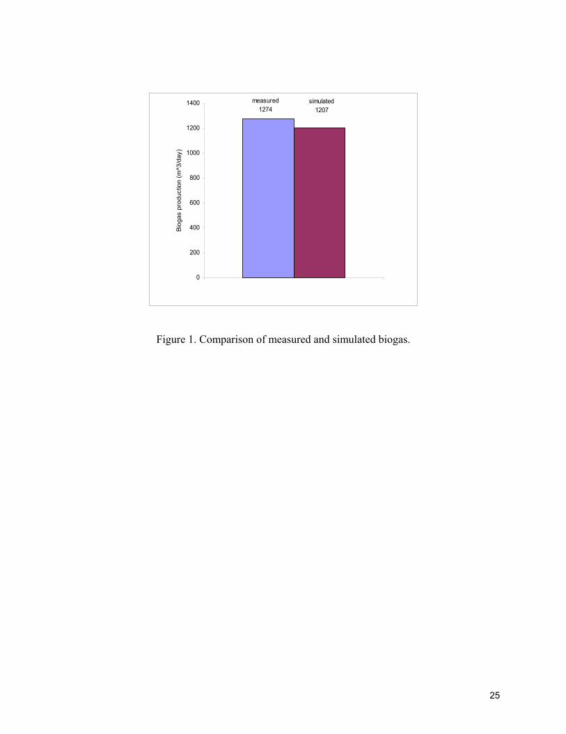
assumed to be 60%, and its density to be 0.6679 3/ mkg . The predicted biogas, 1207 daym /3 , is
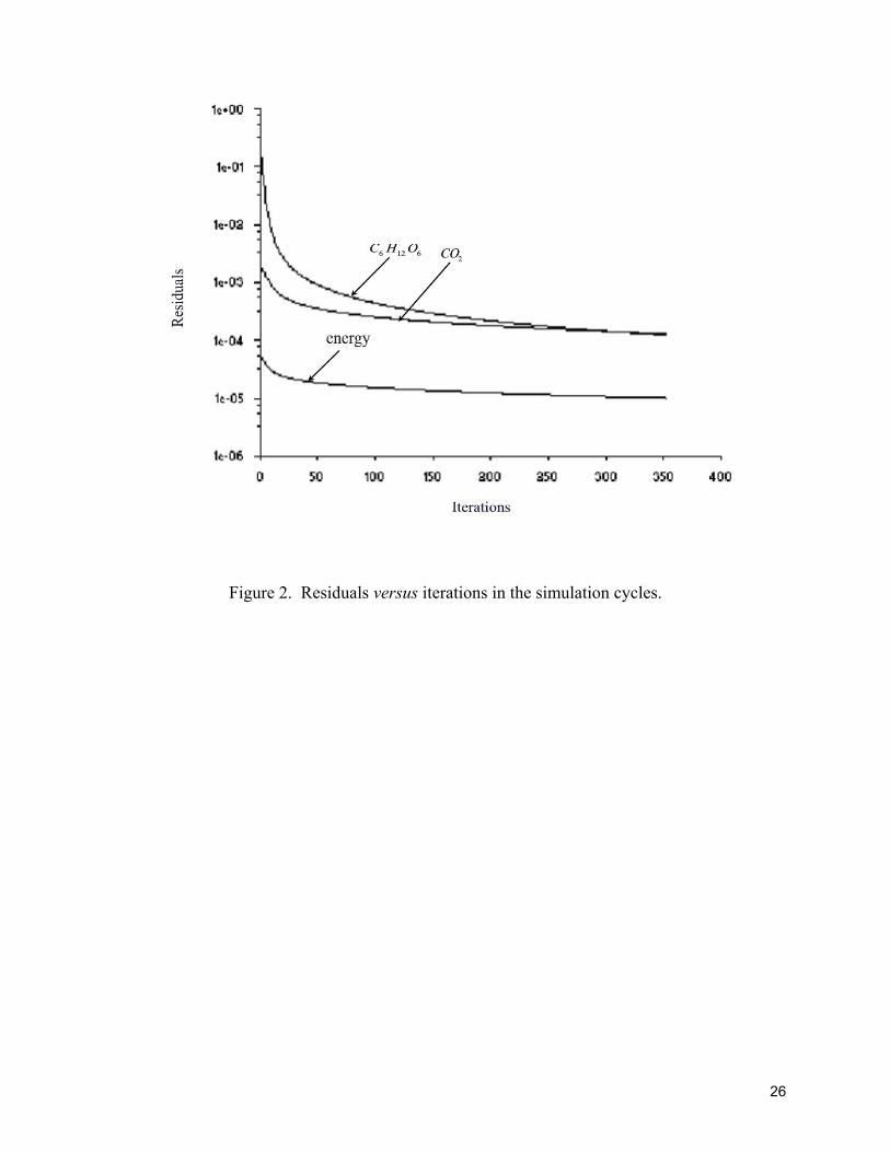
within 5% of measured value, 1274 daym /3 , as shown in Table 1. In the simulation,
convergence occurred after 350 iterations (Figure 2). The convergence criteria were set to be: (1)
that residuals of species is < 3101 −× , and (2) that residual of energy is < 5101 −× . The
calculation trend was steady and without any fluctuations.
17
In this study, the momentum equations and turbulent model are not considered in calculating
biogas predictions because flow velocity of liquid manure in the digester is very low. The
prediction calculations are based on the principles of mass conservation, energy, and species
transport. For this reason, there are only three curves shown in Figure 2 – one for energy, and
two for species transport. The two species are 6126 OHC and 2CO . The sum of mass fractions of
all species is equal to one. For example, if there are N species in the chemical reaction, the Nth
mass fraction is determined by [ ∑−
=
−1
11
N
iiY ]. In this simulation, N =3 since there are only three
species ( 6126 OHC , 2CO , and 4CH ), where 4CH is set as the Nth (3rd) species.
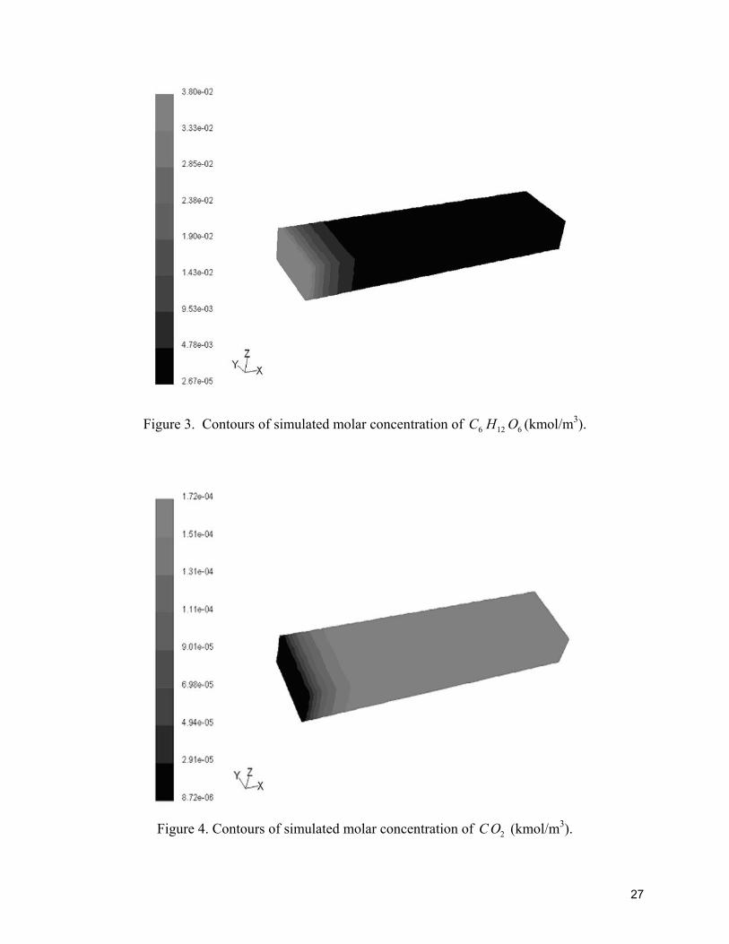
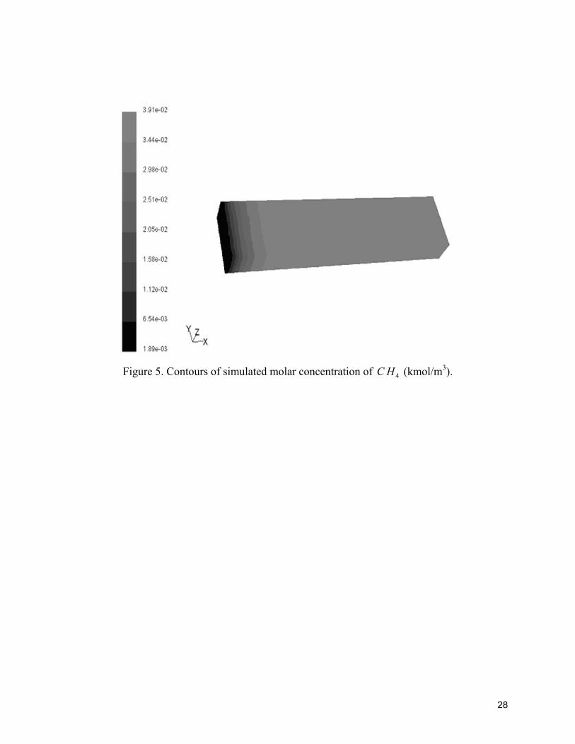
The range of molar concentrations for the three species, 6126 OHC , 4CH and 2CO , are:
51067.2 −× - 21080.3 −× , 61072.8 −× - 41072.1 −× , and 31089.1 −× - 21091.3 −× kmol/m3,
respectively. The simulated contours of the molar concentrations for the three species are given
in Figures. 3, 4, and 5.
From Fig. 3, it can be observed that the concentration of the organic material ( 6126 OHC ) is high
close to the inlet, and low far from the inlet. The concentration also remained unchanged after a
certain distance (about one-sixth of length) from the inlet. The reason is that chemical reaction
gradually develops from the inlet to the outlet. From Figs. 4 and 5, it is evident that the
distributions of 4CH concentrations and 2CO concentrations are similar. However, the actual
values of 4CH is higher than that of 2CO because CH4 is the main product of the chemical
reaction. Similarly, the concentrations of 4CH and 2CO increased gradually from the inlet to
one-sixth the length and then remained unchanged up to the outlet.
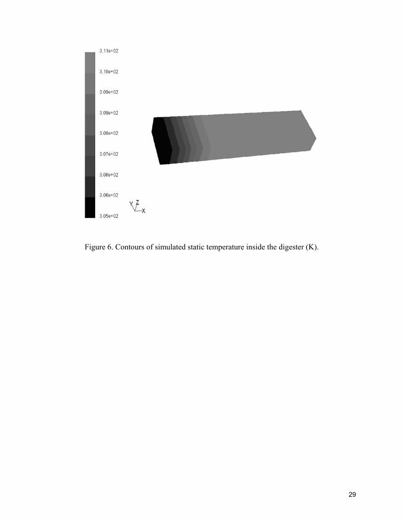
The temperature profile within the digester is given in Fig. 6. The inlet temperature is 305K
(32 C0 ), which is the assumed boundary condition temperature, and the outlet temperature is 311
K (38 C0 ). Temperature profile exists because of chemical reaction taking place when the
reactants (organic material and water) are mixing.
18
Conclusions The following conclusions can be drawn from the study:
(1) A comprehensive literature review on modeling biogas production from anaerobic digestion
was conducted.
(2) A general three-dimensional numerical simulation model that predicts biogas production
from plug-flow type digesters is developed. The model is based on the principles of mass
conservation, energy balance, species transport, and chemical reactions.
(3) Model prediction for a plug-flow anaerobic digester is validated against experimental data
obtained from the literature. The results agree within 5%.
19
References
1. Andara, A. R., and J.M.L. Esteban. 1999. Kinetic study of the anaerobic digestion of the
solid fraction of piggery slurries. Biomass and Bioenergy. 17: 435-443.
2. Axaopoulos, P., P. Panagakis, A. Tsavdaris, and D. Georgakakis. 2001. Simulation and
experimental performance of a solar-heated anaerobic digester. Solar Energy. 70 (2):
155-164.
3. Bryant, M. P. 1979. Microbial methane production-theoretical aspects. Journal of
Animal Science. 48 (1): 193-201.
4. Blumensaat, F., and J. Keller. 2005. Modeling of two-stage anaerobic digestion using the
IWA Anaerobic Digestion Model No.1 (ADM1). Water Research. 39: 171-183.
5. Buswell, A.M., and H. F. Mueller. 1962. Mechanisms of methane fermentations.
Industrial Engineering Chemistry. 44: 550.
6. Chang, F.H. 2004. Energy and sustainability comparisons of anaerobic digestion and
thermal technologies for processing animal waster. ASAE/CSAE meeting, paper No:
044025.
7. Converti, A., A. D. Borghi, S. Arni, and F. Molinari. 1999. Linearized kinetic models for
the simulation of the mesophilic anaerobic digestion of pre-hydrolyzed woody wastes.
Chemical Engineering Technology. 22 (5): 429-437.
20
8. Costello, D. J., P. F. Greenfield, and P. L. Lee. 1991 a. Dynamics modeling of a single-
stage high-rate anaerobic reactor─ I. Model derivation. Water Resource. 35 (7): 847-858.
9. Costello, D. J., P. F. Greenfield, and P. L. Lee. 1991 b. Dynamics modeling of a single-
stage high-rate anaerobic reactor─ II. Model verification. Water Resource. 35 (7): 859-
871.
10. Chen Y., and Hashimoto. 1978. Kinetic of methane fermentation. Proceedings of
Symposium on Biotechnology in Energy Production and Conservation. Scott C. D (Ed.),
John Wiley, New York.
11. Fischer, J. R., E. L. Iannotti, and J. H. Porter. 1984. Anaerobic digestion of swine manure
at various influent solids concentrations. Agricultural Wastes. 11: 157-166.
12. Fluent. 2005. Fluent 6.1. Lebanon, N.H.: Fluent, Inc.
13. Gebremedhin, K.G., B. Wu, C. Gooch, and P. Wright. 2004. Simulation of heat transfer
for maximum biogas production. ASAE/CSAE meeting, paper No: 044165.
14. Harikishan J., and S. Sung. 2003. Cattle waste treatment and class A biosolid production
using temperature-phased anaerobic digester. Advances in Environmental Research. 7:
701-706.
15. Hashimoto A. G. 1983. Thermophilic and mesophilic anaerobic fermentation of swine
manure. Agricultural Waste. 6: 175-191.
21
16. Hashimoto A. G. 1984. Methane from swine manure: effect of temperature and influent
substrate concentration on kinetic parameter (K). Agricultural Waste. 9: 299-308.
17. Hashimoto A. G., Chen Y. R., and Varel V. H. 1981. Theoretical aspects of methane
production: state-of-the-art. In livestock Wastes: A renewable Resource, ASAE, St.
Joseph, MI, 86-91.
18. Hashimoto A. G., T. G. Edgar, and H . Nakano. 1994. Methane production from animal
wastes. Journal of Soil and Water Conservation. 49 (2): 62-68
19. Hill D.T. 1982a. Design of digestion systems for maximum methane production.
Transactions of the ASAE. 25: 226-230.
20. Hill D.T. 1982b. Optimum operational design criteria for anaerobic digestion of animal
manure. Transactions of the ASAE. 25: 1029-1032.
21. Hill D.T. 1982c. A comprehensive dynamic model for animal waste methanogenesis.
Transactions of the ASAE. 25: 1374-1380.
22. Hobbs, P. J., R. Johnson, and D. Chadwick. 1999. A novel technique to determine
organic processes in pig waste. Journal of the Science of Food and Agriculture. 79: 199-
205.
23. Jewell, W.J., H.R. Carpener, S. Dell'orto, K.J. Fanfoni, T.D. Hayes, A.P. Leuschner, T.L.
Miller, D.F. Sherman, P.J.V. Soest, M.J Wolin, and W.J. Wujcik. 1978. Anaerobic
fermentation of agricultural residue: Potential for improvement and implementation -
22
Final Report. Technical Report EY-76-S-02-2981-7, Cornell University/US Department
of Energy.
24. Karim, K., K. T. Klasson, R. Hoffmann, S. R. Drescher, D. W. Depaoli, and M. H. Al-
Dahhan. 2005. Anaerobic digestion of animal waste: effect of mixing. Bioresource
Technology. 96: 1607-1612.
25. Kayhanian M., and G. Tchobanoglous. 1996. Development of a mathematical model for
the simulation of the biodegradation of organic substrates in high-solids anaerobic
digestion process. Journal of Chemical Technology and Biotechnology. 66: 312-322.
26. Keshtkar, A., B. Meyssami, G. Abolhamd, H. Ghaforian, and M. K. Asadi. 2003.
Mathematical modeling of non-ideal mixing continuous flow reactors for anaerobic
digestion of cattle manure. Bioresource Technology. 87: 113-124.
27. Magnussen, B.F., and B. H. Hjertager. 1976. On mathematical models of turbulent
combustion with special emphasis on soot formation and combustion.
In 16th Symp. (Int'l.) on Combustion. The Combustion Institute.
28. McGrath R. J, and I. G. Mason. 2004. An observational method for the assessment of
biogas production from an anaerobic waste stabilization pond treating farm dairy
wastewater. Biosystems Engineering. 87 (4): 471-478.
29. Metcalf and Eddy. 2003. Wastewater Engineering (fourth edition). McGraw-Hill, New
York.
23
30. Minott, S.J. 2002. Feasibility of fuel cells for energy conversion on the dairy farm.
Thesis. Cornell University, Ithaca, NY.
31. Masse D. I., and R.L. Droste. 2000. Comprehensive model of anaerobic digestion of
swine manure slurry in a sequencing batch reactor. Waste Research. 34 (12): 3087-3106.
32. Patankar, S.V. 1980. Numerical Heat Transfer and Fluid Dynamics, Hemisphere/
McGraw-Hill, New York.
33. Pavlostathis S.G., and J. M. Gossett. 1986. A kinetic model for anaerobic digestion of
biological sludge. Biotechnology and Bioengineering. 28:1519-1530.
34. Safely, L.M., Jr, and P.W. Westerman. 1992. Performance of a low temperature lagoon
digester. Bioresource Technology. 41: 167-175.
35. Safely, L.M., Jr, and P.W. Westerman. 1994. Low-temperature Digestion of dairy and
swine manure. Bioresource Technology. 47: 165-171.
36. Toprak, H. 1995. Temperature and organic loading dependency of methane and carbon
dioxide emission rates of a full-scale anaerobic waste stabilization pond. Water Research.
29 (1): 1111-1119.
37. Vartak, D.R., C.R. Engler, S.C. Ricke, and M.J. Mcfarland. 1999. Low temperature
anaerobic digestion response to organic loading rate and bioaugmentation. Journal of
Environmental Science and Health. A34(3): 567-583.

24
Table 1. Input information and comparison of measured and predicted results1.
Digester dimension
Measured biogas
production
(m3/day)
Simulated
biogas
production
( daym /3 )
Error
(%)
Length
(m)
Width
(m)
Depth
(m)
39.62
9.44
4.26
1274
1207
5.25
1Measured biogas production is from AA Dairy Farm, Homer, NY (Gebremedhin et al., 2004)
Daily manure flow rate =38.336 m3/day
HRT = 3590906 s (41 days and 13 hrs)
Retention temperature = 32 C0
25
measured 1274
simulated 1207
0
200
400
600
800
1000
1200
1400
Bio
gas
prod
uctio
n (m
^3/d
ay)
Figure 1. Comparison of measured and simulated biogas.
26
Figure 2. Residuals versus iterations in the simulation cycles.
27
Figure 3. Contours of simulated molar concentration of 6126 OHC (kmol/m3).
Figure 4. Contours of simulated molar concentration of 2OC (kmol/m3).
28
Figure 5. Contours of simulated molar concentration of 4HC (kmol/m3).
29
Figure 6. Contours of simulated static temperature inside the digester (K).