three-dimensional multispecies distribution … · learned more than they know. i hope miguel...
TRANSCRIPT

THREE-DIMENSIONAL MULTISPECIES DISTRIBUTION FUNCTIONS INA PLASMA BOUNDARY WITH AN OBLIQUE MAGNETIC FIELD
Derek S. Thompson
Dissertation submitted to the Eberly College of Arts and Sciencesat West Virginia University
in partial fulfillment of the requirements for the degree of
Doctor of Philosophyin
Physics
Earl E. Scime, Ph.D., ChairAmy M. Keesee, Ph.D.Paul A. Cassak, Ph.D.
Timothy N. Good, Ph.D.
Department of Physics and Astronomy
Morgantown, West Virginia2018
Keywords: boundary layers, presheaths, laser induced fluorescence, helicon,radio-frequency, velocity distribution functions
Copyright 2018 Derek S. Thompson


Abstract
THREE-DIMENSIONAL MULTISPECIES DISTRIBUTION FUNCTIONS INA PLASMA BOUNDARY WITH AN OBLIQUE MAGNETIC FIELD
Derek S. Thompson
In many plasma-based technologies, the plasma-facing vessel surface plays a largepart in determining the lifetime of the plasma device. Plasma interactions withits containment vessel are unavoidable, and are often benign, but in devices withhigh thermal loading — as in magnetically-confined fusion experiments — or withlong operational lifetimes without maintenance — such as spacecraft thrusters —these interactions take on critical importance to the viability of the technology.The severity of plasma-material interactions is determined by the material itselfand by the plasma boundary in contact with it. The organization and dynamicsof the particles in this region are old problems, however major questions remain,especially with respect to the reorganization of plasma boundaries in the presenceof magnetic fields.
In this document, the physics of a weakly magnetized boundary region are inves-tigated. A boundary is created by immersing a ?76.2 mm stainless steel disk in ahelicon plasma that emulates many thruster- and fusion-relevant plasma parame-ters. Here, the velocity distributions of ions and neutral particles are mapped ina plasma boundary region, created in 3.6 mTorr argon gas, 650 W RF power, andmagnetic field B = 0.06 T, where the magnetic field lines obliquely intersect thewall (↵ = 16�). These distributions are mapped using laser induced fluorescencein three spatial (3D) and three velocity (3V) dimensions, and reveal that modelsneglecting any one of the velocity components omit important components of theflow field. Electrostatic probe measurements are presented, and establish a typi-cal helicon plasma discharge with electron temperature Te ⇡ 4.2 eV and densityn ⇡ 5.5 ⇥ 1017 m�3. In addition to the observed ion temperature, Ti ⇡ 0.37 eV,these measurements indicate a plasma in which the electrons are highly magnetized(!ce/⌫e = 2.9⇥ 103) and the ions are weakly collisional (!ce/⌫i = 0.5± 0.3).
Ion drift velocity measurements are presented in the E ⇥ B direction and com-pared to predictions from measured plasma potential gradients. Ion flow fieldsare compared to predictions from collisional fluid simulations and particle-in-cellmodels conducted by Rinat Khaziev and Davide Curreli at the University of Illi-nois at Urbana Champaign. These models require ion-neutral collisions to predictthe ion drifts well. Neutral particle distributions are observed to be in thermalequilibrium with the chamber walls (Tn ⇡ 0.028 eV) and essentially non-flowingon average. Charge exchange populations are expected to be O(10�2), and are toosmall to be resolved, but are excluded to the 5% level.

Acknowledgements
This is my attempt at thanking in a sentence or two people who have shaped mylife to this point and continue to do so. Many people have had my back. To evenlist names would take many pages and I’m bound to miss someone. Nevertheless,here we go.
I want to first express my gratitude for the support of my advisor, Earl Scime, whosmoothed my way to WVU and who for the last two and half years has trusted mewith his lab probably more than he had reason to. His students, myself certainly,too often underappreciate the freedom he affords us. He has answered annoyingquestions at 7 am and after midnight, and was available for lunch almost everyday I’ve been in Morgantown. That kind of face-to-face relationship building isexceptional and not lost on me. He is a mentor and a friend.
Enormous gratitude to Davide Curreli, Rinat Khaziev, and Shane Keniley at theUniversity of Illinois Urbana-Champaign, and to Umair Siddiqui, with whom I’veworked since early in my time at Madison. They were instrumental in laying thefoundations of this project and saw it through. In particular, I want to thankRinat, who is always patient with my flood of questions, and Umair, whose recentwork provided the inspiration for this work. Without them the project would havebeen something less.
I thank Amy Keesee, who brought me on as a collaborator for her work at NASA,provided much-needed expertise in argon neutral atomic physics to that compo-nent of this project, wrote a dissertation that I refer to constantly, and showedme mercy after I temporarily disabled the interaction interface of her Tesla whileon the highway. I would like to thank Timothy Good for his good company, hu-mor, advice, and insightful challenges, which were greatly appreciated and enjoyedduring long data campaigns. In addition to graciously agreeing to serve on mycommittee, Paul Cassak has been an extremely valuable resource and teacher eversince I arrived at WVU. I am fortunate to have met and worked with all of mythesis committee members. Again: thank you.
I would like to thank Ray Fonck, Dave Smith, George McKee, and Noah Her-shkowitz, my advisors at the University of Wisconsin-Madison, along with thestaff and students of the Pegasus Toroidal Experiment in Madison and NSTXin Princeton. Greg Winz and Cyrus Nourgostar taught me an enormous amountthat has been repeatedly useful. Out of everyone I’ve worked with, I have probablyendangered them most, and they always approached the work with good humor.
My undergraduate advisors — Nicolas Dauphas, Josh Frieman, Juan Estrada,Emily Nurse, and Young-Kee Kim — always supported me beyond what my earlyefforts probably deserved. They are all exceptional scientists whom I attempt toemulate in various ways. I see much of their guidance in the best parts of the workI’m presenting here.

J.R. Raber, Doug Mathess, and Carl Weber helped design and fabricate the intri-cate components of the test boundary and several diagnostics. They entertainedliteral fever dreams during this project and made it happen. Viola Bryant, SherryPuskar, and Beena Bhanushali expertly cleared away distractions and were alwayspatient with me.
The students whom I’ve worked with during my time at WVU — Mikal Dufor,Takeru Furukawa, Jacob McLaughlin, Andrew Jemiolo, Luke Neal, Xiao Zhang,Zachary Short, Julianne McIlvain, Yujian Zhao — have all contributed to thisproject or have in some way helped me prepare for this work. Many of them wereinvolved in the considerable data acquisition stage. Drew Elliott never let mesettle; Dave Caron props me up with his chemistry and material science insightsand encyclopedic knowledge of funny things; Thomas Steinberger is an invaluablesounding board and motivator; Evan Aguirre shared HELIX/LEIA without vio-lence and generously included me in some of his research; and John McKee hadthe bravery to wade into deep Langmuir probe theory with me. From them I havelearned more than they know. I hope Miguel Henriquez and Mindy Bakken, withwhom I’ve worked closely, find that they too have derived some benefit from ourcollaboration. I am proud to call them colleagues and friends.
The long journey through a PhD is made possible only through good friends. Iconsider myself exceptionally fortunate to have attended Madison at the sametime as Umair Siddiqui, one of the best leaders and explorers I believe I’ll meet.The same is true for Corey Henderson, who knows where and how to look, and forJaime and Niall, co-navigators through shipwrecks galactic and lacustrine. MattMichalak is an exceptional creator, not to mention an excellent fellow traveler.Adam Ernst, who in every space knows what’s good. And Neil Lutz, with whomI have collaborated, I hope, on something like equal terms.
Sarah and Neil have always been encouraging on rough days, silly on easy days,and good company always. I attribute my enjoyment of knowledge and pursuit ofunderstanding to my parents, who have encouraged blending curiosity with hardwork since my memory begins. They set it all in motion and deserve more creditthan they can ever get.
Finally, I want to thank Marisa, my ally and accomplice. She is the kernel andthe sum.
Thank you all.

Contents
Abstract ii
Acknowledgements iii
List of Figures viii
List of Tables xi
Abbreviations xii
1 Motivation and context 1
1.1 The Science . . . . . . . . . . . . . . . . . . . . . . . . . . . . . . . 11.1.1 Weakly collisional presheaths in oblique magnetic fields . . . 3
1.2 The engineering . . . . . . . . . . . . . . . . . . . . . . . . . . . . . 51.3 The helicon as a plasma boundary test bed . . . . . . . . . . . . . . 7
1.3.1 Comparison of the HELIX helicon source to other plasmas . 71.3.2 Heating and plasma production in helicon plasmas . . . . . 81.3.3 Density, temperature, and rotation profiles in HELIX . . . . 161.3.4 Neutral depletion in the plasma core . . . . . . . . . . . . . 19
1.4 Thesis overview . . . . . . . . . . . . . . . . . . . . . . . . . . . . . 22
2 Experimental Apparatus 23
2.1 The HELIX/LEIA facility . . . . . . . . . . . . . . . . . . . . . . . 232.1.1 ⇡ network matching circuit . . . . . . . . . . . . . . . . . . . 25
2.2 Absorbing boundary . . . . . . . . . . . . . . . . . . . . . . . . . . 292.3 Boundary coordinates . . . . . . . . . . . . . . . . . . . . . . . . . . 31
2.3.1 Translation stage coordinates . . . . . . . . . . . . . . . . . 322.3.2 Simulation coordinates . . . . . . . . . . . . . . . . . . . . . 34
3 Diagnostics 36
3.1 Gaussmeter . . . . . . . . . . . . . . . . . . . . . . . . . . . . . . . 363.2 Langmuir probes . . . . . . . . . . . . . . . . . . . . . . . . . . . . 39
3.2.1 Langmuir probe construction . . . . . . . . . . . . . . . . . 393.2.2 Langmuir probe circuit . . . . . . . . . . . . . . . . . . . . . 423.2.3 Langmuir probe analysis . . . . . . . . . . . . . . . . . . . . 47
v

Contents vi
3.2.3.1 Introduction . . . . . . . . . . . . . . . . . . . . . 473.2.3.2 Calculation of the fluid quantities ni, ne, and Te . . 503.2.3.3 EDFs, EEDFs and EEPFs . . . . . . . . . . . . . . 583.2.3.4 Other considerations . . . . . . . . . . . . . . . . . 71
3.2.4 Electrostatic fluctuations . . . . . . . . . . . . . . . . . . . . 753.3 Laser induced fluorescence . . . . . . . . . . . . . . . . . . . . . . . 76
3.3.1 Overview . . . . . . . . . . . . . . . . . . . . . . . . . . . . 763.3.2 Velocity distributions from LIF data . . . . . . . . . . . . . 783.3.3 Optical arrangement . . . . . . . . . . . . . . . . . . . . . . 793.3.4 Conventional LIF . . . . . . . . . . . . . . . . . . . . . . . . 823.3.5 Confocal LIF . . . . . . . . . . . . . . . . . . . . . . . . . . 853.3.6 Ar-I LIF . . . . . . . . . . . . . . . . . . . . . . . . . . . . . 913.3.7 Ar-II LIF . . . . . . . . . . . . . . . . . . . . . . . . . . . . 963.3.8 Other considerations . . . . . . . . . . . . . . . . . . . . . . 98
4 Three-dimensional, multispecies measurements in a boundary with
an oblique magnetic field: B = 600 G, = 74� 107
4.1 Introduction . . . . . . . . . . . . . . . . . . . . . . . . . . . . . . . 1074.2 Magnetic field measurements . . . . . . . . . . . . . . . . . . . . . . 1084.3 EEPF, ne, Teff, and pe from Langmuir probe measurements . . . . . 109
4.3.1 Non-Maxwellian features are observed in EEPFs . . . . . . . 1104.3.2 The helicon source creates a radial density gradient . . . . . 1114.3.3 Teff distribution reflects high-energy electron populations . . 1124.3.4 pe = nekBTe shows a radial helicon electron pressure gradient 113
4.4 �p depends on proximity to the boundary surface . . . . . . . . . . 1144.5 Ion temperature and pressure, Ti(x,v) and pi(x,v), distributions
from LIF data . . . . . . . . . . . . . . . . . . . . . . . . . . . . . . 1144.5.1 Ti is slightly anisotropic . . . . . . . . . . . . . . . . . . . . 1144.5.2 The ion pressure is isotropic: pi(x,v) ⇡ pi(x) . . . . . . . . 1164.5.3 Characteristic velocities in the boundary . . . . . . . . . . . 118
4.6 Characteristic frequencies in the boundary . . . . . . . . . . . . . . 1184.7 The metastable Ar-II drift velocities measured by LIF show a 3D
flow field . . . . . . . . . . . . . . . . . . . . . . . . . . . . . . . . . 1284.8 Testing Chodura’s model . . . . . . . . . . . . . . . . . . . . . . . . 1314.9 Comparison of HELIX boundary data with collisional fluid and
Particle-in-Cell simulations . . . . . . . . . . . . . . . . . . . . . . . 1354.10 Ion-neutral collisions in the presheath . . . . . . . . . . . . . . . . . 1414.11 Characterizing the drift in the E⇥B direction . . . . . . . . . . . . 144
5 Conclusions 147
A Digital smoothing of signals 150
A.1 Overview . . . . . . . . . . . . . . . . . . . . . . . . . . . . . . . . . 150

Contents vii
A.2 Moving average . . . . . . . . . . . . . . . . . . . . . . . . . . . . . 151A.3 Gaussian convolution . . . . . . . . . . . . . . . . . . . . . . . . . . 152A.4 Blackman window convolution . . . . . . . . . . . . . . . . . . . . . 154A.5 Savitzky-Golay filtering . . . . . . . . . . . . . . . . . . . . . . . . . 154A.6 Summary of results . . . . . . . . . . . . . . . . . . . . . . . . . . . 156
Bibliography 158

List of Figures
1.1 Non-Maxwellian features observed in ion distributions in an unmag-netized sheath . . . . . . . . . . . . . . . . . . . . . . . . . . . . . . 4
1.2 Poloidal cross section of ITER tokamak . . . . . . . . . . . . . . . . 51.3 Anomalous erosion observed in Hall thruster channels . . . . . . . . 61.4 Comparison of plasma quantities: DIII-D SOL, BHT-600 Hall thruster,
HELIX . . . . . . . . . . . . . . . . . . . . . . . . . . . . . . . . . . 81.5 Density dependence on magnetic field magnitude showing mode
transitions in a helicon . . . . . . . . . . . . . . . . . . . . . . . . . 121.6 Electric field patterns in a helicon . . . . . . . . . . . . . . . . . . . 131.7 Propagating helicon mode structures . . . . . . . . . . . . . . . . . 131.8 Energetic electron populations observed in HELIX . . . . . . . . . . 141.9 Te, n, and Ti vs fRF and B in HELIX . . . . . . . . . . . . . . . . . 151.10 Images of mode structure in CSDX . . . . . . . . . . . . . . . . . . 161.11 Power spectra of electrostatic fluctuations in HELIX . . . . . . . . . 171.12 Radial Ti profile . . . . . . . . . . . . . . . . . . . . . . . . . . . . . 181.13 LIF intensity profile in HELIX . . . . . . . . . . . . . . . . . . . . . 181.14 Azimuthal and radial flow profiles in HELIX . . . . . . . . . . . . . 191.15 Heatmap of plasma column rotation in HELIX . . . . . . . . . . . . 191.16 Axial flow dependence on magnetic field in CSDX and HELIX . . . 201.17 HELIX Ar-I density and ion-neutral collision rate profiles . . . . . . 211.18 Kr-I density profiles and dependences in CHEWIE . . . . . . . . . . 21
2.1 Overview schematic of the HELIX chamber . . . . . . . . . . . . . . 242.2 Circuit diagram: ⇡ matching circuit . . . . . . . . . . . . . . . . . . 262.3 HELIX load and tuning capacitor ranges . . . . . . . . . . . . . . . 282.4 Photograph of the (Type 316) stainless steel absorbing boundary . . 292.5 Photograph detail of the (Type 316 SS) laser beam dump . . . . . . 302.6 Photograph of the absorbing boundary immersed in the HELIX
plasma . . . . . . . . . . . . . . . . . . . . . . . . . . . . . . . . . . 312.7 Magnetic field perturbation from boundary . . . . . . . . . . . . . . 312.8 Diagram of coordinate systems . . . . . . . . . . . . . . . . . . . . . 322.9 Limits of experimental domain . . . . . . . . . . . . . . . . . . . . . 332.10 LIF & LP measurement locations . . . . . . . . . . . . . . . . . . . 34
3.1 Gaussmeter magnetic field orientation . . . . . . . . . . . . . . . . . 383.2 HELIX cutaway showing probe translation mechanism . . . . . . . 41
viii

List of Figures ix
3.3 Langmuir probe electrode on translation stage . . . . . . . . . . . . 413.4 Langmuir probe circuit diagram . . . . . . . . . . . . . . . . . . . . 423.5 Input and output frequency sweeps for Langmuir and emissive probes. 473.6 Bode plot for Langmuir and emissive probes . . . . . . . . . . . . . 473.7 Probe characteristic showing: I. ion saturation, II. transition region,
III. electron saturation. . . . . . . . . . . . . . . . . . . . . . . . . . 493.8 Example conventional Langmuir probe analysis . . . . . . . . . . . 533.9 OML analysis I
2� V plot . . . . . . . . . . . . . . . . . . . . . . . 55
3.10 range for Te = 4 eV and B = 600 gauss . . . . . . . . . . . . . . . 653.11 range for rp = 250 µm and `p = 2 mm . . . . . . . . . . . . . . . 663.12 Example EEPF calculated using conventional Druyvesteyn analysis 673.13 Example EEPF calculated using strongly magnetized analysis . . . 683.14 I
00e
reconstructed using extended Druyvesteyn analysis . . . . . . . . 693.15 Dependence of K 00 and on relative potential. . . . . . . . . . . . . 693.16 PSD of �f . . . . . . . . . . . . . . . . . . . . . . . . . . . . . . . . 763.17 Example IVDF measured in p = 3.5 mTorr, PRF = 650 W, B = 600
G plasma . . . . . . . . . . . . . . . . . . . . . . . . . . . . . . . . 793.18 Sirah Matisse DR LIF optical arrangement . . . . . . . . . . . . . . 803.19 Diagram of 3D stage . . . . . . . . . . . . . . . . . . . . . . . . . . 833.20 Ray trace diagram of 3D stage optics . . . . . . . . . . . . . . . . . 843.21 Diagram of axial injection stage . . . . . . . . . . . . . . . . . . . . 853.22 Diagram of axial injection placement on HELIX . . . . . . . . . . . 863.23 Ray trace diagram of confocal optics . . . . . . . . . . . . . . . . . 873.24 Diagram of confocal deployment on HELIX . . . . . . . . . . . . . . 873.25 Temperature and mean flow profiles measured by conventional and
confocal LIF . . . . . . . . . . . . . . . . . . . . . . . . . . . . . . . 893.26 Confocal beam profiles for f = 150 mm . . . . . . . . . . . . . . . . 903.27 Relative metastable density profiles measured by conventional and
confocal LIF . . . . . . . . . . . . . . . . . . . . . . . . . . . . . . . 903.28 Grotrian diagram for metastable Ar-I LIF . . . . . . . . . . . . . . 933.29 Typical Ar-I spectra showing Zeeman splitting . . . . . . . . . . . . 943.30 Ar-I spectral width laser power dependence . . . . . . . . . . . . . . 953.31 Ar-I spectrum recorded parallel to the magnetic field . . . . . . . . 963.32 Dependence of Zeeman-split cluster separation on B . . . . . . . . . 973.33 Transition diagram for metastable Ar-II LIF . . . . . . . . . . . . . 973.34 Example overintegration of VDFs . . . . . . . . . . . . . . . . . . . 1003.35 Overintegration trend in mean velocity for scan time selection . . . 1003.36 IVDF series showing laser reflections . . . . . . . . . . . . . . . . . 1023.37 Beam profiles for Matisse laser . . . . . . . . . . . . . . . . . . . . . 104
4.1 Detail of the coordinate systems showing the plasma shift . . . . . . 1084.2 Hall effect probe measurements of Bk = By⇤ . . . . . . . . . . . . . 1084.3 EEPF dependence on plasma radius and axial location . . . . . . . 1104.4 ne(x) in the boundary region . . . . . . . . . . . . . . . . . . . . . . 1114.5 Electron density and temperature dependence on z . . . . . . . . . 112

List of Figures x
4.6 Teff(x) in the boundary region . . . . . . . . . . . . . . . . . . . . . 1124.7 Spatial structure of the electron pressure, pe . . . . . . . . . . . . . 1134.8 Electron and ion pressure dependence on z . . . . . . . . . . . . . . 1134.9 Measured �p(x) in the boundary region . . . . . . . . . . . . . . . . 1144.10 Ti(x,v⇤) in 3D3V . . . . . . . . . . . . . . . . . . . . . . . . . . . . 1154.11 Spatial variation of pi(x,v) . . . . . . . . . . . . . . . . . . . . . . . 1174.12 Experimental ion collision cross-sections . . . . . . . . . . . . . . . 1214.13 Experimental �CX and �SC [124], with ⌫CX and ⌫SC . . . . . . . . . . 1214.14 Dependence of KIZ and ⌫IZ on nn and Te . . . . . . . . . . . . . . . 1224.15 Neutral depletion on-axis in HELIX . . . . . . . . . . . . . . . . . . 1234.16 Dependence of ln� on Te, Ti and n . . . . . . . . . . . . . . . . . . 1244.17 Dependence of Coulomb collision frequencies on Te, Ti and ne ⇡ ni . 1254.18 3D map of Ar-II metastable drift velocities from LIF data . . . . . 1284.19 Data showing decrease in uz near boundary before interpolation . . 1304.20 vz distribution function cascade with distance to the boundary surface1304.21 Comparison between ui measurements in MARIA and Chodura’s
prediction . . . . . . . . . . . . . . . . . . . . . . . . . . . . . . . . 1314.22 Comparison of predicted and observed �mps . . . . . . . . . . . . . . 1324.23 3D heatmap of Bohm-Chodura boundary . . . . . . . . . . . . . . . 1334.24 3D projection of Bohm-Chodura boundary . . . . . . . . . . . . . . 1344.25 Total flow minus field-parallel flow approaching the boundary surface1354.26 Comparison of data and simulations . . . . . . . . . . . . . . . . . . 1374.27 Normalized uy and uz as functions of ux . . . . . . . . . . . . . . . 1394.28 Mean axial flow of 1s5 metastable Ar-I . . . . . . . . . . . . . . . . 1404.29 Large scale axial potential structure observed in the MARIA exper-
iment . . . . . . . . . . . . . . . . . . . . . . . . . . . . . . . . . . . 1414.30 ux dependence on neutral pressure in simulations . . . . . . . . . . 1424.31 Metastable Ar-I velocity distribution evolution with proximity to
the wall . . . . . . . . . . . . . . . . . . . . . . . . . . . . . . . . . 1434.32 Comparison of Ar-I and Ar-II spectra at close proximity to the wall 1444.33 uz for three fill pressures . . . . . . . . . . . . . . . . . . . . . . . . 1454.34 uz for three fill pressures . . . . . . . . . . . . . . . . . . . . . . . . 145
A.1 Comparison of probe characteristics smoothed by moving average . 152A.2 Comparison of window widths used in moving average smoothing . 152A.3 Comparison of Gaussian smoothed probe characteristics . . . . . . . 153A.4 Comparison of several � used in Gaussian smoothing . . . . . . . . 153A.5 Comparison of probe characteristics smoothed by Blackman filtering 154A.6 Comparison of window widths used for Blackman filtering . . . . . 155A.7 Comparison of probe characteristics smoothed by Savitzky-Golay
filtering . . . . . . . . . . . . . . . . . . . . . . . . . . . . . . . . . 156A.8 Comparison of window widths used for Savitzky-Golay filtering . . . 156

List of Tables
2.1 HELIX facility engineering parameters . . . . . . . . . . . . . . . . 232.2 HELIX facility plasma quantities . . . . . . . . . . . . . . . . . . . 25
3.1 RF choke specifications used in Langmuir probe compensation circuit 453.2 DS345 settings for electrostatic probe frequency response measure-
ments . . . . . . . . . . . . . . . . . . . . . . . . . . . . . . . . . . 463.3 Scale lengths in a sample helicon plasma in HELIX . . . . . . . . . 623.4 Summary of the Langmuir probe results for a sample characteristic 723.5 HELIX chamber dimensions and typical plasma conditions . . . . . 743.6 Summary of Ar-I metastable 4s[2P 0
3/2]2 (1s5) LIF schemes withVIS/NIR transitions . . . . . . . . . . . . . . . . . . . . . . . . . . 92
3.7 Summary of Ar-I metastable 4s[2P 03/2]2 (1s5) Zeeman effect . . . . . 95
3.8 Approximate transmission coefficients of elements in the LIF opticaltrain . . . . . . . . . . . . . . . . . . . . . . . . . . . . . . . . . . . 104
3.9 Response function parameters . . . . . . . . . . . . . . . . . . . . . 105
4.1 Fiducial measurements for �Ti(stat.) . . . . . . . . . . . . . . . . . 1174.2 Characteristic velocities . . . . . . . . . . . . . . . . . . . . . . . . 1194.3 Plasma and cyclotron frequencies for both charged species . . . . . 1194.4 Collision frequencies for measured range of Te, Ti, and n . . . . . . 127
A.1 Summary of digital smoothing techniques . . . . . . . . . . . . . . . 157
xi

Abbreviations
3D Three orthogonal spatial dimensions
3V Three orthogonal velocity dimensions
ABR Allen, Boyd, and Reynolds
APC Angled physical contact (fiber connector)
Ar-I Neutral argon gas
Ar-II Single-ionized argon
AWG American wire gauge
BHT Busek Hall effect Thruster
BNC Bayonet Neill-Concelman (connector/standard)
BRL Bernstein, Rabinowitz, and Laframboise
CCD Charge-coupled device
CL Child-Langmuir
CR Collisional-Radiative model
CSDX Controlled Shear Decorrelation Experiment
CSV Comma separated variable
CX Charge exchange
DR Dye ring
EDF Electron distribution function
EEDF Electron energy distribution function
EEPF Electron energy probability function
EG Ethylene glycol
EI Electron-ion Coulomb scattering
EMI Electromagnetic interference
EP Emissive probe
xii

Abbreviations xiii
EPH Ethylene glycol monophenyl ether
FC Ceramic ferrule (fiber connector)
FWHM Full-width at half-maximum
GaAs Gallium arsenide
HELIX Hot hELIcon eXperiment
ID Inner diameter
IE Ion-electron Coulomb scattering
II Ion-ion Coulomb scattering
InAs Indium arsenide
ITER International Thermonuclear Experimental Reactor
IV Current-voltage (trace)
IVDF Neutral velocity distribution function
IZ Ionization
Kr-I Neutral krypton gas
Kr-II Singly-ionized krypton
LASER Light Amplification by Stimulated Emission of Radiation
LEIA Large Experiment on Instabilities and Anisotropies
LIF Laser induced fluorescence
LP Langmuir probe
MARIA Magnetized AnisotRopic Ion-distribution Apparatus
MCC Monte-Carlo collisions
MM Multimode (fiber)
MPEX Material Plasma Exposure eXperiment
MPS Magnetic presheath
NIST National Institute of Standards and Technology
NSTX National Spherical Torus Experiment
NVDF Ion velocity distribution function
OD Outer diameter
OML Orbital motion limited
PEEK Polyether ether ketone
PIC Particle-in-Cell

Abbreviations xiv
PMT Photo-multiplier tube
PPPL Princeton Plasma Physics Laboratory
PSD Power spectral density
PTFE Polytetrafluoroethylene
RAID Resonant Antenna Ion Device
RDW Resistive drift wave
RF Radio-frequency
RFEA Retarding field energy analyzer
RMS Root-mean squared
RMSE Root-mean squared error
SC Elastic scattering
SM Single mode (fiber)
SMA SubMiniature version A
SNR Signal-to-Noise Ratio
SOL Scrape-off layer
TALIF Two photon absorption laser induced fluorescence
UIUC University of Illinois at Urbana-Champaign
VASIMR Variable Specific Impulse Magnetoplasma Rocket
VDF Velocity distribution function
WVU West Virginia University

Chapter 1
Motivation and context
1.1 The Science
The importance of the boundary region to the total plasma discharge has been
recognized nearly as long as plasmas have been studied. Early plasma physicists
reasoned that the long range electromagnetic forces in almost all plasmas would
eventually contact an interface, creating a boundary region termed a "sheath,"
and that this boundary region, though small, would impact the global plasma
equilibrium [1]. As Hershkowitz succinctly argued: "sheaths matter" [2]. The
physics of plasma boundaries is interesting because advances in understanding
assist technology development, as discussed in Sec. 1.2, but also because sheaths
and sheath-like structures occur in natural plasma phenomena as far ranging as
lightning [3] and planetary plasma sheets [4].
Early plasma experiments by Langmuir and Bohm demonstrated that in unmagne-
tized systems the particles passing through the boundary would experience several
regions. In the bulk plasma, far from the boundary, any local electric fields created
by boundaries or other distant causes are shorted out by the plasma’s high electri-
cal conductivity. At the surface or just above it, the higher electron flux — at least
when Te > Ti, for electron and ion temperatures respectively — charges the surface
to a negative potential relative to the bulk plasma, and the sheath ceases to be
1

Motivation and context 2
quasineutral. The potential structure in the sheath repels additional low-energy
electrons and attracts ions, until the ion and electron fluxes settle into an equilib-
rium. The constant fluxes through a stable sheath require the ion velocity toward
the wall to become supersonic, i.e. v � cs.=
p(�iTi + �eTe)/mi, a condition that
has become known as the Bohm criterion [5]. If ions in the bulk are not moving on
average and are supersonic in the sheath, then a region, termed the "presheath,"
is required in which they accelerate. Within the presheath, the potential gradient
is gradual over a long distance and quasineutrality still holds. Significant progress
has been made toward understanding sheath and presheath behavior, extending
simple boundary conditions to plasmas with multiple ion species [6], biased elec-
trodes [7], and near small or large electrodes with respect to the chamber diameter
[8], to name a very small subset.
A restructuring of the boundary region occurs with the introduction of a magnetic
field. In highly magnetized plasmas, where the gyro-frequency exceeds the collision
rate, particles in the bulk plasma tend to follow magnetic fields lines. The geometry
becomes highly anisotropic, with transport along field lines dominating transport
across field lines. In the opposite extreme, where the magnetic field is very weak,
the plasma conditions revert to the magnetic field-less case.
For intermediate fields, particles transition from a region where the magnetic field
dominates, far from the boundary, to one in which they interact with both the
anisotropic magnetic field and strong gradients in the plasma potential. These
fields interact to produce nonlinear behavior and are further complicated by the
host of collisions that arise as particles from the plasma and particles at the in-
terface intermingle. These effects conspire to create a plasma that is three dimen-
sional and potentially non-Maxwellian. Theoretical and computational investiga-
tions that attempt to replicate particle motion in these boundaries are challenging.
Models must describe the gradual spatial variations of the presheath and the sharp
gradients of the sheath; the long time-scale behavior such as ion or neutral thermal
drifts and fast electron behavior; and often the non-thermal distribution functions
that result from inelastic collisions. All of these features require additional com-
putational expense, and omitting some of them in the interest of computational

Motivation and context 3
expediency can easily result in inaccuracies. Determining which features should
be neglected and which ones are essential is one aim of using experimental obser-
vations to validate codes.
1.1.1 Weakly collisional presheaths in oblique magnetic fields
Chodura [9] is typically credited with initiating the study of presheaths in oblique
magnetic fields, when the angle, , between the normal vector of the interface and
the magnetic field lines is nearly 90�. In this model, the plasma behaves like a
fluid and only the spatial and drift velocity components along the surface normal
are resolved. Collisions are neglected, as are finite gyro-radius effects, and the ions
are assumed to follow an isotropic Maxwellian distribution. Chodura proposed a
new region of the boundary, which he called the "magnetic presheath," in which
the plasma was still quasi-neutral, but where the electric field of the boundary is
sufficient to cause particles to deflect from their magnetic field-parallel trajectories.
In this “Chodura layer,” the ions are supersonic parallel to the magnetic field,
but are not yet supersonic normal to the wall. A classical “plasma presheath”
accelerates the ions to the uk � cs condition. The boundary of the Chodura layer
is established by a modified criterion, referred to as the Bohm-Chodura criterion,
which states that the ion flow toward the boundary must become supersonic, but
reduced according to the magnetic angle:
1 > ux/cs � cos .
He predicted that this condition would be satisfied at a distance
�mps =p6(cs/!ci) sin
from the Debye sheath edge. In the limit that the magnetic field and the surface
normal are aligned, ! 0, the Chodura layer vanishes, and the Bohm criterion
is recovered.

Motivation and context 4
Since that time, magnetic presheath research has enjoyed broad theoretical progress
[10–16]. Only a few experiments exist in literature to provide data to validate these
models [17–22]. Of these experiments, the early focus was on mapping the plasma
potential structure of the boundary region with electrostatic probes. Siddiqui et
al. were the first to report measurements of argon ion distribution functions and
2D flow fields in a boundary with 60� [21], which they compared to a colli-
sional fluid model. Preliminary results related to the experiments reported in this
dissertation were described two years later in Ref. [22]. Early measurements of
ion drifts in the direction parallel to E⇥B were reported for the first time.
Measurements of the background metastable neutral population were unavailable
to the authors of Refs. [21] and [22]. Through elastic scattering collisions, ion-
ization, and charge exchange, ion and neutral populations modify each other’s
distribution functions. Collisionality depends on the relative drifts of the two
populations, and even a coarse neutral flow measurement is useful for constrain-
ing collisional models. More detailed distribution measurements provide velocity
distribution data on the neutral population and reveal the presence of any non-
Maxwellian collisional markers such as charge exchange [23]. Such non-Maxwellian
distributions are observed in unmagnetized sheaths (see Fig. 1.1). Metastable neu-
Figure 1.1: Non-Maxwellian features observed in ion distributions in anunmagnetized sheath [23].
trals, especially the 1s5 state described in more detail in Sec. 3.3.6 and in [24],
Motivation and context 5
make up a large fraction of the total neutral population and have long state life-
times, making them advantageous for measuring the transient conditions of the
boundary.
1.2 The engineering
The implications of magnetic presheath physics extend into engineering and tech-
nological applications. Sheaths in magnetic environments appear around space-
craft antennae [25] and terrestrial diagnostic probes [26]. Magnetic confinement
fusion devices, such as tokamaks, use strong magnetic fields to divert particles and
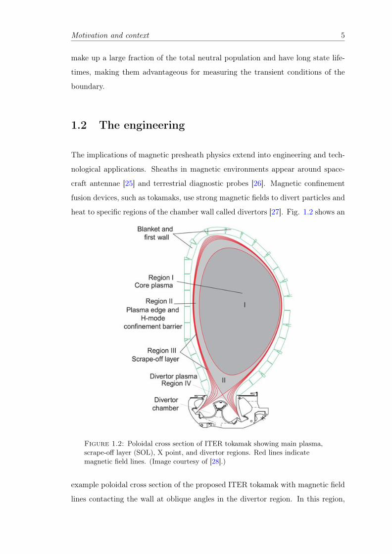
heat to specific regions of the chamber wall called divertors [27]. Fig. 1.2 shows an
Figure 1.2: Poloidal cross section of ITER tokamak showing main plasma,scrape-off layer (SOL), X point, and divertor regions. Red lines indicatemagnetic field lines. (Image courtesy of [28].)
example poloidal cross section of the proposed ITER tokamak with magnetic field
lines contacting the wall at oblique angles in the divertor region. In this region,

Motivation and context 6
careful shaping of the magnetic field distributes the extreme particle and heat loads
over a large area to reduce concentrations of particle flux and power. Particle and
heat fluxes modify the surface and the plasma in several ways. Sputtering and
erosion caused by particle bombardment changes the shape of the wall over time,
and depend, among other things, on the ion energy, flux, and impact angle [29].
In the process, some of the wall material returns to the plasma. Wall material is of
higher mass and atomic number relative to the plasma — walls are often carbon
(ZC = 6), molybdenum (ZMo = 42), or tungsten (ZW = 74), compared to the
hydrogen (ZH = 1) or helium (ZHe = 2) plasma — and because these elements
are more easily ionized, power losses from the lighter species occur. Gas particles
trapped in the lattice of the wall material are released, affecting gas fueling control
and plasma shaping in the edge. Heat and particle fluxes are determined in part
by the boundary regions that separate the chamber wall from the hot bulk plasma
[15, 29, 30].
Recently, Siddiqui et al. argued that magnetic presheath physics might explain
anomalous erosion rates observed in Hall thruster channels (see Fig. 1.3 [22]).
Hall thruster channel erosion sets up the conditions for the main failure mode of
Figure 1.3: Anomalous erosion observed in Hall thruster channels duringlifetime tests. (Image presented in [22], courtesy of M. Gamero-Castano and I.Katz [31].)
Hall thrusters [32], and reducing it is critical for extending thruster operational
lifetimes. Recent order-of-magnitude lifetime extensions have been achieved in
magnetically shielded Hall thrusters [32, 33]. This extension is attributed to a

Motivation and context 7
modification of the potential structure by channel and magnetic field shaping,
which effectively reduces the flux and impact energy of ions at the channel wall.
It is worth mentioning that the popular Hall thruster modeling Particle-in-Cell
code HPHall does not include ion drifts in the E ⇥ B direction, which Siddiqui
et al. argue may account for discrepancies between Hall thruster simulations and
experiments [22].
1.3 The helicon as a plasma boundary test bed
1.3.1 Comparison of the HELIX helicon source to other
plasmas
As a plasma source, helicons have a high degree of variability, operate in capac-
itive, inductive, and helicon modes, and produce plasma densities over a range
from approximately 1015 � 1019 m�3. While the mechanism is a subject of on-
going experiment, the high efficiency of helicon plasma production is well know
and even allows them to create plasmas with densities that approach the densities
in tokamak divertors using merely hundreds of watts. Fig. 1.4 shows a compari-
son of plasma parameters between the DIII-D scrape-off-layer, the BHT-600 Hall
thruster, and HELIX.
The magnetic fields in HELIX are on the same order as the representative BHT-
600 Hall thruster and at the lower end of the range for the high aspect ratio DIII-D
scrape-off-layer. Low aspect ratio spherical tokamaks have magnetic fields on the
order of the fields in HELIX [36–38]. The primary difference between the devices
is the ion temperature, which in tokamaks can be comparable to the electron
temperature. The two effects partially cancel in setting the ion gyroradius in
HELIX, and it is therefore slightly smaller than in the tokamak SOL.
Several high-power helicons are currently in operation or development. These de-
vices have wide-ranging applications, from interplanetary spacecraft propulsion

Motivation and context 8
Figure 1.4: Comparison of plasma quantities: DIII-D SOL, BHT-600 Hallthruster, HELIX. Table presented in [22]. Original data from [34] and [35].
(VASIMR [39]) to material testing and beam generation for fusion devices (Proto-
MPEX [40]; RAID [41]). These devices will build on our understanding of mag-
netized plasma boundaries and extend them to new high-powered regimes.
1.3.2 Heating and plasma production in helicon plasmas
A history of the helicon wave
The helicon discharge was first named in the early 1960s by Aigrain, who was
studying wave propagation in indium [42, and references]. Early theoretical work
was pioneered by Legendy [43], Formato and Gilardini [44], and Klozenberg, Mc-
Namara and Thonemann [45]. Reviews of the early development of helicons can
be found in [46]. The study of the family of low-frequency (! ⌧ !pe) waves to
which helicon waves belong, called whistler waves, is historically interesting, as
it involves eavesdropping on poorly secured communications during World War
I. Interpretations of whistler wave signals, which were initially observed at audi-
ble frequencies, varied from "the grenades fly" to Martian communications [46].
The whistler wave phenomenon was later ascribed to the propagation of charged
particles along the Earth’s magnetic field lines following lightning strikes [47].

Motivation and context 9
The helicon wave was observed in a toroidal plasma in 1960 [48]. Since that time, it
has been developed for use at a range of frequencies [49], antenna shapes [50, 51,
and references], and RF powers [52–55], and applied to plasma processing [56],
spacecraft propulsion [57, 58], and laboratory science experiments [59]. Recent
developments are reviewed in [60–62].
The helicon dispersion relation
The helicon is a low-frequency, radially bounded whistler wave propagating in a
magnetic field. (The discussion in this section follows [60, 63, 64] with background
support from [65, 66].) It is useful to describe each physical quantity as the sum of
a background component and a perturbation component, such that n = no + �n,
E = Eo + �E, etc., with the assumption that the perturbed quantity is much
smaller than the background. The most significant behavior is described by the
0th and 1st order quantities, so that e.g. �n�v ⇠ 0. The background fields are
assumed to be static, have magnitude Bo and direction z, and [66]:
rno = vo = 0@no
@t=@vo
@t=@Eo
@t=@Bo
@t.
Quasineutrality dictates that neo ⇡ nio, and in the cold plasma approximation
(Te ⇠ Ti ⇠ 0) �ni ⇡ 0. The wave is assumed to be a plane wave propagating
in a cylindrical waveguide. Each perturbed quantity is assumed to be sinusoidal
in space and time (r, t), with frequency ! and wavenumber k / 2⇡/�, so that
�E = Eo exp(ik ·r�!t), etc. In this framework, the full set of Maxwell’s equations
are
r · �E = e�ne/✏o r · �B = 0
r⇥ �E = �@�B
@tr⇥ �B = µo�J+ ✏oµo
@�E
@t, (1.1)
in SI, where B[T] is the magnetic field, J[A/m2] the current density, ne[m�3] the
electron density, and E[V/m] the electric field. For singly-charged ions J0 = 0.
From now on, all ordering subscripts will be dropped and all quantities will be

Motivation and context 10
assumed to be perturbations unless otherwise indicated. Using Ohm’s law with a
conductivity tensor �, i.e. without assuming that the current density is directed
along E, J = � · E, and Ampere’s law in Eq. (1.1) is
r⇥B = µo
✓� · E+ ✏o
@E
@t
◆= µo
✓� · E� i!✏oE
◆
= �i!
c2
✓I�
�
i!✏o
◆· E.
I is the identity tensor. The quantity in parentheses is the effective dielectric
tensor, ✏R (in some places K), where the dielectric tensor ✏ = ✏o✏R. The curl of
Faraday’s law is
r⇥ (r⇥ E) = r⇥
✓�@B
@t
◆= �
@
@t
⇥r⇥B
⇤
r(r · E)�r2E = �
@
@t
� i
!
c2
✓I�
�
i!✏o
◆· E
�
�k(k · E) + k2E =
!2
c2✏R · E.
k2c2
!2
✓kk
k2� I
◆+ ✏R(!,k)
�· E = 0.
i.e. [67, Eq. 9.55]
det����k2c2
!2
✓kk
k2� I
◆+ ✏R(!,k)
���� = 0. (1.2)
In the cold plasma approximation, this condition simplifies to [65]
det
���������
S � n2 cos2 ✓ �iD n
2 cos ✓ sin ✓
iD S � n2 0
n2 cos ✓ sin ✓ 0 P � n
2 sin2✓
���������
= 0, (1.3)

Motivation and context 11
which results in the cold plasma dispersion relation
An4� Bn
2 + C = 0 (1.4)
where
A = S sin2✓ + P cos2 ✓
B = RL sin2✓ + PS(1 + cos2 ✓)
C = PRL.
If the background magnetic field is taken to be aligned with z, the axis of the
machine, so that B = Boz, then ✓ is defined by the perpendicular, parallel, and
total wavenumbers:
✓ ⌘ arccos(kk/k).
The solutions to Eq. (1.4) are [65]
tan2✓ =
P�n2�R
��n2� L
��Sn2 �RL
��n2 � P
�
For propagation along the background field, k ! kk, ✓ ! 0, either P = 0, in
which only plasma oscillations exist; n2 = R, and propagation occurs with right-
handed polarization when looking parallel to B; n2 = L, and propagation occurs
with left-handed polarization. Helicon waves form a subset of the right-handed
polarization case, which for a single ion argon plasma have [65],
n2R =
k2c2
!2=
!2pe
!ce!�1 + !ci/! � !/!ce
� (1.5)
For helicons, !ci ⌧ ! ⌧ !ce ⌧ !pe, and Eq. (1.5) becomes
k2c2
!2=
!2pe
!ce!. (1.6)

Motivation and context 12
In physical quantities,
ne =k2
!
B
eµo
(1.7)
and the wave propagates with wavelength �[m] = 5.6 ⇥ 1012(B/nefRF)1/2 [68],
with wave frequency, f = !/2⇡, in Hz. Eq. (1.7) indicates a linear dependence
on the magnetic field magnitude and frequency [69]. In experiments, the density
has been shown to follow this prediction, however helicons exhibit distinct mode
transitions in which the density increases sharply at a threshold field magnitude
(see Fig. 1.5).
Figure 1.5: Density dependence on magnetic field magnitude showing modetransitions [68].

Motivation and context 13
Mode structures in helicons
The propagating helicon mode field structures have been calculated by Chen [62].
The m = ±1 electric field patterns are shown in Fig. 1.6. The m = -1 mode is
narrower and propagates less effectively. The mode rotates as it propagates down
Figure 1.6: Electric field patterns in a helicon [62]. The m = -1 mode isnarrower and propagates less effectively.
the cylinder, as shown in Fig. 1.7.
Figure 1.7: Propagating helicon mode structures as seen by a stationaryobserver [62].
Progress in understanding helicon source heating and efficiency
(This subsection borrows from the discussion in [61].) As early as the 1960s scien-
tists began to suspect that something was missing in the early description of the
efficient energy transfer between the helicon wave and the plasma. The heating

Motivation and context 14
could not be entirely attributed to collisional damping of the helicon waves or to
Landau damping of energetic electrons [70], however axially streaming energetic
electron populations have been observed (Fig. 1.8 [71]).
Figure 1.8: Energetic electron populations observed in HELIX [71].
The ability to vary RF frequency in helicon experiments has opened the possibility
of testing the frequency-dependence of helicon heating. In parts (a) and (c) of Fig.
1.9, the lower hybrid frequency, !LH sets a clear threshold for an increase in Te.
In part (b), the maximum densities are observed at !LH, and generally increase
for increasing !LH. These observations clearly show a dependence on !LH which
is not a part of the helicon dispersion relation in Eq. (1.6). The challenge is
to reconcile two phenomena: 1) In many sources, the majority of the RF power
transfer appears directly under the forward edge of the antenna, indicating an
effect local to the antenna; however 2) "blue core" helicons have been observed in
equilibrium several meters downstream of the antenna, suggesting electromagnetic
energy propagation along the plasma column.
The underlying physics depends, in an as-yet incompletely understood way, on the
radial geometry and transport of the plasma and on the axial boundary conditions.
In recent experiments, low-frequency resistive drift wave (RDW) instabilities in
regions of strong radial density gradients separate two other plasma regions: 1) a

Motivation and context 15
Figure 1.9: Te, n, and Ti vs fRF and B in HELIX [72]. The white line marksthe on-axis lower hybrid frequency.
bright core with a rotating mode and 2) a turbulent edge. Radial transport occurs
in opposing directions in 1) and 2), establishing a transport barrier in the region
where the RDW instabilities dominate. This transport barrier sets the radial
boundary of the blue core [73] (Fig. 1.10). In the same device, changing the the
boundary conditions between insulating and conducting materials 2.8 m from the
antenna was sufficient to change plasma potential profiles, rotation profiles, and
the Reynold’s stress [74]. The axial boundary conditions modified radial currents,
and drastically changed fluctuation characteristics [74, 75]. In addition, spectral
sidebands, markers of parametrically driven fluctuations, have been observed in
electrostatic fluctuation spectra at different RF frequencies, as shown in Fig. 1.11
[72].
Measurements of ion temperature anisotropy in helicons suggests strong ion heat-
ing in the edge in the direction perpendicular to the background magnetic field
[72]. The helicon edge is characterized by low densities, which correspond to lower
!LH in the edge than in the center of the column. It is possible that that perpen-
dicular slow wave modes arise in densities low enough to allow Landau damping on
the ions. In this way, ion heating propagates radially from edge heating, and is not
primarily caused by wave-particle interactions with fast electrons [61]. Needless
to say, the details of the underlying mechanisms involved remain the subject of
much-needed investigation.

Motivation and context 16
Figure 1.10: Images of mode structure in CSDX [73]. Blue core not observedin (b). Blue core mode shown in (d), with visible coherent structures out to afinite radius r ⇡ 3 cm, after which plasma edge is turbulent.
1.3.3 Density, temperature, and rotation profiles in HELIX
Experiments using helicons for source plasmas must separate the effects of the
gradients within the plasma column from gradients established by the boundary.
Fig. 1.13 compares the laser-induced fluorescence (LIF) signal intensity profile
from metastable argon ions to the profile of neT1/2e [76]. The two profiles show
remarkable agreement given the simplicity of the dependence.
Radial electric fields generate rotation of the plasma column, as shown in Fig. 1.14.
In (a), the azimuthal ion flow changes sign near the mechanical axis of the machine
and slows at larger radii. The ions exhibit negligible radial flows. The rotation
rate varies significantly for different plasma conditions. Compare, for example,
the plasma rotation in Fig. 1.14 to the measurements in Fig. 1.15, which show a

Motivation and context 17
Figure 1.11: Power spectra of electrostatic fluctuations in HELIX showingsidebands [72].
2D rotation map of perpendicular ion drifts at greater magnetic field magnitude
and lower pressure. The ions in the core exhibit little drift, however within a few
centimeters they acquire speeds of several hundred m/s. The rotation speed and
profile are observed to depend on the magnetic field magnitude [77]. Ti is shown
in (b) to be relatively uniform over the innermost part of the plasma, r . 3 cm.
Axial ion flows in the CSDX cylindrical helicon source were observed to be several
hundred m/s at fill pressure p = 3.2 mTorr and RF power PRF = 1800 W, as shown
(left) in Fig. 1.16 [78]. At low magnetic field magnitudes, the axial flow profile
is relatively flat. At higher fields, the flow decreases and perhaps changes sign at

Motivation and context 18
Figure 1.12: Radial Ti profile showing anisotropic ion heating at outer radii[72].
Figure 1.13: LIF intensity profile in HELIX, at fRF = 9.5 MHz, PRF = 750W, p = 3.6 mTorr, and B = 716 G [76]. Blue circles show the LIF signalintensity. Red squares show neT
1/2e .
the outermost radii. Three-dimensional ion flows are shown at right in Fig. 1.16,
along with the LIF signal amplitude. In the top plot, the arrows show a rotating
plasma and the color shows an ion population that is streaming along the axis in
an annular shell, in contrast to the CSDX measurements.

Motivation and context 19
Figure 1.14: (a) azimuthal ion measured with LIF, at fRF = 9.5 MHz, PRF= 750 W, p = 3.8 mTorr, and B = 652 G; and (b) radial neutral flows inHELIX, at fRF = 9.5 MHz, PRF = 750 W, p = 34 mTorr, and B = 500 G [76].Axis of symmetry is located at X ⇡ �0.5 cm.
Figure 1.15: Heatmap of plasma column rotation in HELIX, measured withLIF, at fRF = 9.5 MHz, PRF = 750 W, p = 1.8 mTorr, and B = 730 G [76].Arrows indicate ion flow speed. Color indicates LIF intensity in (a) and Ti in(b).
1.3.4 Neutral depletion in the plasma core
Momentum exchange collisions between ions and with neutral particles is an im-
portant component of the physics of plasma boundaries, especially when helicon
sources are used to generate the test plasma. In contrast to primarily azimuthal
and axial ion flows, inward neutral flows across the plasma density gradient are

Motivation and context 20
Figure 1.16: Left: Axial flow dependence on magnetic field in CSDXmeasured with LIF. fRF = 13.65 MHz, PRF = 1800 W, and p = 3.2 mTorr [78].Right: 3D ion flow cross section, including axial flow in color (top), and LIFsignal amplitude (bottom). fRF = 9.5 MHz, PRF = 750 W, B = 652 G, andp = 3.8 mTorr [76].
observed in LIF flow measurements, as shown in part (b) of Fig. 1.14. These in-
ward flows suggest inelastic collisions such as charge exchange or ionization play a
role in establishing the helicon equilibrium [79]. Collision rates depend on the den-
sity of the target species. While local ion densities can be measured by Langmuir
probes, it is difficult to measure absolute neutral densities in argon for estimating
collision rates, and measurable quantities are combined with collisional-radiative
(CR) models to estimate neutral density profiles. An example profile, calculated
using a CR model for a plasma in p = 6.0 mTorr with B = 750 G and PRF = 300
W, is shown in Fig. 1.17 along with the estimated momentum-transfer collision
rate profile [76, 80, 81]. These profiles indicate high ionization or charge exchange
collisions, with neutral depletion of 30-40% in the core at these plasma parameters.
Neutral pressures as low as one-tenth of the pre-discharge fill pressure have been
observed for similar argon plasma conditions [79, 82–84]. As a result, models as-
suming flat profiles and using neutral densities from pressure gauges located in the
chamber wall risk misrepresenting the collision rates at the center of the column.
Absolute densities have been measured in helicon plasmas in krypton in the
CHEWIE device [85]. As expected, they show a linear increase in neutral density

Motivation and context 21
Figure 1.17: Ar-I density and ion-neutral collision rate profiles for B = 750G, PRF = 300 W, p = 6.0 mTorr [76, 80, 81].
with fill pressure, and nn ⇡ 1020 m�3 at p = 3.6 mTorr. At PRF = 600 W, the
neutral density is insensitive to magnetic field magnitude until B � 600 G, above
which the neutral density decreases as the plasma density rises. Plasma and neu-
tral density profiles, and dependence of the Kr-I and Kr-II densities on magnetic
field and fill pressure are shown in Fig. 1.18. At B = 600 G and PRF = 600 W,
Figure 1.18: Kr-I density profiles and dependences in CHEWIE [85]. (a)Pressure dependence of two-photon absorption LIF (TALIF) signal. (b) Kr-Idensity (black triangles, left axis) and Kr-II density (blue diamonds, right axis)profile at fRF = 13 MHz, PRF = 600 W, and B = 600 G. (c) Magnetic fielddependence of Kr-I density (black triangles, left axis) and Kr-II density (bluediamonds, right axis) at PRF = 600 W. (d) r-I density (black triangles, leftaxis) and Kr-II density (blue diamonds, right axis) profile at fRF = 11 MHz,PRF = 800 W, and B = 1200 G.
similar conditions to the measurements reported here, the Kr-II profile is centrally

Motivation and context 22
peaked, but the Kr-I profile is hollow, showing perhaps a 50% neutral depletion
within |r| 1 (See (c), Fig. 1.18).
1.4 Thesis overview
This dissertation describes the measurement of ion, neutral, and electron dynamics
in a boundary region with an oblique magneitc field. Where possible, measure-
ments of all three spatial and three velocity components are acquired. The details
of the boundary that was created to study the magnetic presheath are described in
Chapter 2. Described in this chapter are the coordinate systems used to map the
boundary region. The HELIX facility which provides the consistent test plasma
is described as well, along with a brief description of several key components.
Chapter 3 describes the diagnostics used for the measurements presented. The
3-axis probe is introduced and its construction and calibration methods are de-
tailed. The plasma conditions in the boundary were not known a priori, so a litany
of Langmuir probe analysis methods are described for extracting plasma quanti-
ties from this diagnostic. Several important pitfalls are highlighted. Chapter 3
describes the laser-induced fluorescence technique that was used to measure the
ion and neutral velocity distributions, including transition schemes, calibration,
and a list of possible artifacts. The results from the experimental campaign are
presented in Chapter 4, where they are compared to collisional fluid and Particle-
in-Cell simulations and accompanied by some implications for magnetic presheath
theory. Chapter 5 summarizes the results of the project and provides some addi-
tional discussion.

Chapter 2
Experimental Apparatus
2.1 The HELIX/LEIA facility
The experiments reported here were conducted in the Hot hELIcon eXperiment
(HELIX) attached to the Large Experiment on Instabilities and Anisotropies
(LEIA) facility at West Virginia University. For this work, the HELIX/LEIA ex-
periment is used primarily as a plasma source, however its primary objective and
resources make it an attractive device for studying plasma boundaries. A schematic
of the HELIX chamber is shown in Fig. 2.1 and typical ranges for engineering quan-
tities are listed in Tab. 2.1. A recent review of the facility is available in Ref. [59],
which contributes to much of this discussion.
The HELIX chamber consists of a ?10 cm x 63 cm cylindrical Pyrex tube situated
between a ?15 cm x 91 cm stainless steel tube and a Pyrex cross. The end of the
Parameter Typical Minimum MaximumfRF [MHz] 9.5 0.3 30PRF [W] 650 0 2000B [T] 0.06 0 0.12Mass flow [sccm] 20 0.1 200Pump rate [L/s] 3200 0 3750
Table 2.1: HELIX facility engineering parameters[59].
23

Experimental Apparatus 24
Figure 2.1: Overview schematic of the HELIX chamber.
stainless steel section opposite the Pyrex attaches coaxially to LEIA, a 4 m long, 2
m diameter aluminum expansion chamber. A uniform magnetic field up to 0.12 T
(1225 G), with field variation �B/B . 1% is established in HELIX by ten water-
cooled copper channel pancake electromagnets driven by a parallel pair of Xantrex
XFR DC power supplies.
Optical access to the HELIX plasma is provided by sixteen 2.75" Conflat ports,
spaced 6" apart at top, bottom, and both sides of the HELIX chamber. At the
ports nearest the antenna, static telescopes with fiber ports maintain a fixed,
optimized focus on the center of the plasma. This optical arrangement is used
for standard measurements and troubleshooting. Halfway down the length of the
HELIX chamber, a 6" Conflat cross-port provides large volume optical and probe
access to the plasma. This is the location of most of the experiments reported in
this document.
Vacuum in the chamber is maintained by a 550 L/s turbomolecular pump attached
to the bottom of the Pyrex cross and two 1600 L/s turbomolecular drag pumps
on the rear wall of LEIA. Each of these pumps is backed by an oil-free diaphragm
pump. The large chamber volume is reduced from atmospheric pressure to 0.5 Torr
by an oil-free roots pump. This vacuum system ensures that the surfaces inside

Experimental Apparatus 25
Parameter Typical Minimum Maximumn [m�3] 5⇥ 1018 ⇠ 5⇥ 1015 ⇠ 3⇥ 1019
TAr-I [eV] 0.027 0.025 -TAr-II [eV] 0.4 0.15 2.5Te [eV] 4 1.5 15pvac [Torr] 1⇥ 10�7 7⇥ 10�8 5⇥ 10�7
pgas [mTorr] 4 0.1 100
Table 2.2: HELIX facility plasma quantities [59].
the chamber are never exposed to pump oil. The chamber readily obtains vacuum
pressures below 5⇥ 10�7 Torr, a pressure that improves to 7� 8⇥ 10�8 Torr after
several hours of steady plasma operation.
Gas is typically fed into the chamber from the top of the Pyrex cross, however
a second port partway down the stainless steel section is available for injection
as well. Plasmas in HELIX are formed from argon, helium, nitrogen, hydrogen,
xenon, and krypton gases. Gas flow is controlled with calibrated MKS 1179 mass
flow valves and a MKS PR-4000 mass flow controller. The mass flow operates from
a minimum of 0.1 sccm up to 200 sccm. The pressure inside HELIX is manipulated
by the mass flow controller, the location of gas injection, and by opening or closing
the gate valves to the vacuum pumps. Pre-plasma fill pressures range from 0.1 to
100 mTorr.
Plasmas in HELIX are created by a 19 cm long, half wave, m = +1 helical antenna,
which is wrapped around the cylindrical Pyrex section of the chamber. The antenna
is driven at RF frequencies between 8.5 and 16 MHz. Up to 1.5 kW of forward RF
power is produced by a single ENI A1000 RF power supply, driven by a Wavetek
80 function generator. Typical plasma conditions are shown in Tab. 2.2.
2.1.1 ⇡ network matching circuit
RF power is coupled to the plasma by driving the antenna through a balanced ⇡
network matching circuit. A diagram of the matching circuit on HELIX is shown

Experimental Apparatus 26
in Fig. 2.2. In a ⇡ network matching circuit, neither side of the antenna is electri-
Figure 2.2: Circuit diagram: HELIX ⇡ matching circuit [59]. The loadcapacitor is placed in parallel with the antenna. Three tuning capacitors areplaced in series with the antenna.
cally connected to ground. One side of the antenna is separated from the ground
reference by three tuning capacitors in parallel with each other. Two of these ca-
pacitors are Jennings UCSL 250 tunable capacitors with a 4-250 pF range. The
other capacitor is a Jennings UCSL 500 tunable capacitor with a 5-500 pF range.
These tuning capacitors allow RF power to be driven over a theoretical range of
0.3 - 30 MHz, however the RF frequency for all measurements reported here is 9.5
MHz. The side of the antenna away from the tuning capacitor set is connected
to the negative pole of the power supply. The load capacitor, a Jennings CVCD
2000 tunable capacitor with a 20-2000 pF range and 40 A maximum current, is
connected parallel to the antenna and the power supply on the side of the tuning
capacitors away from the antenna. The capacitors connect to the antenna and the
power supply via a 6.2 mm thick silver-plated copper bar, which serves as a strong
electrical connection, mechanical support, and heat sink [59].
The goal of a ⇡ network matching circuit is to create a (50 + 0i) ⌦ impedance
that matches the impedance of the transmission lines, minimizing the reflected
power. (The following discussion adapts [86].) The impedance should be entirely
real. The impedance of the circuit, with the tuning capacitors combined into a

Experimental Apparatus 27
single quantity CT and the load capacitance CL, is
Z =�Z
�1L + Z
�1T )
��1 (2.1)
where ZL = 1/i!CL, ZT = R + iX + 1/i!CT, and ! is the RF driving frequency.
X is the reactance of the antenna and changes depending on whether the load is
primarily inductive or capacitive. Inserting ZL and ZT into Eq. (2.1), and defining
Q = X � 1/!CT:
Z =
i!CL +
1
R + iX + 1/i!CT
��1
=R + i(X � 1/!CT)
1 + i!CL[R + i(X � 1/!CT)]
=R + iQ
1� !CLQ+ i!RCL. (2.2)
Making the denominator purely real the impedance becomes
Z =(R + iQ)(1� !CLQ� i!RCL)
(1� !CLQ)2 + (!RCL)2=
R� i⇥!CL(R2 +Q
2)�Q⇤
(1� !CLQ)2 + (!RCL)2
= =R� i
⇥!CL(R2 +Q
2)�Q⇤
1� 2!CLQ+ (!CL)2(R2 +Q2). (2.3)
Im(Z) = 0 implies !CL(R2 +Q2)�Q = 0, or equivalently
(!CL)2(R2 +Q
2) = !CLQ. (2.4)
Eq. (2.3) can now be rewritten to match Re(Z) = Ro:
!CLQ = 1�R/Ro (2.5)
If A ⌘ !CLQ, solving the quadratic in Eq. (2.4) gives
2A� 1 = ±(1� 4!2C
2LR
2)1/2
(1� 2R/Ro)2 = 1� 4!2
C2LR
2.

Experimental Apparatus 28
Therefore
CL =1
2!R
1�
✓1�
2R
Ro
◆2�1/2(2.6)
and from Eq. (2.5)
CT =
!X �
1�R/Ro
CL
��1
(2.7)
For a helicon discharge, X is expected to be primarily inductive, so that X =
XL = !L. In this case, Eq. (2.7) becomes C�1T = !
2L� (1� R/Ro)/CL. At large
L, the purely resistive term dominates and the matching doesn’t depend strongly
on the inductance of the antenna and the circuit establishes a stable discharge.
In practice, the capacitors are tuned to achieve this condition. Fig. 2.3 shows the
predicted range required for the HELIX load capacitor. The 20 - 2000 pF HELIX
load capacitance is appropriate for antenna resistances above approximately 1.4
⌦, and CT < 1000 pF is appropriate above approximately 0.4 µH. In essence, for
a given antenna, the capacitor set determines the range of frequencies over which
a stable discharge can be sustained. In the discharges used in the experiments
Figure 2.3: HELIX ⇡ matching circuit load and tuning capacitance for arange of antenna resistance and inductance. The 20 - 2000 pF HELIX loadcapacitance is appropriate for antenna resistances above approximately 1.4 ⌦.The tuning capacitance is weakly dependent on the antenna resistance, andCT < 1000 pF is appropriate above approximately 0.4 µH.
reported in this document, which are created in 3.6 mTorr of argon, a magnetic
field of 600 gauss, and an RF frequency of 9.5 MHz, the HELIX matching circuit
is capable of reducing the reflected RF power below < 3 W out of 650 W.

Experimental Apparatus 29
2.2 Absorbing boundary
The test boundary in these experiments, shown in Fig. 2.4, is created from a 1
Figure 2.4: Photograph of the (Type 316) stainless steel absorbing boundary.
mm thick, ?7.62 cm Type 316 stainless steel disk. The boundary dimensions are
intended to be large enough that the behavior observed at the center will not be
influenced by edge effects, since the distance between the sample region to the
edge is larger than the sheath and presheath scales, the charge exchange length,
and the ion and electron gyroradii. The disk is fixed to a U-shaped Type 316
bracket that supports the disk and prevents it from sagging or deflecting. The
bracket also provides a strong electrical connection between the disk and the post
that grounds the disk to the chamber wall through a low-impedance path. The
impedance between the outer edge of the disk and the nearby flange is measured
with a digital multimeter to be less than the tip-to-tip impedance of the probes,
i.e. < 0.3 ⌦. Rotating the post outside the chamber changes the angle between the
boundary within the optical access at the center of the cross port.
At the center of the disk, a razor blade beam dump sits within a ?9.5 mm hole
so that the edges of the blades are flush with the disk surface. The beam dump
is used to attenuate false “signals” from laser reflection off the boundary surface
during laser-induced fluorescence (see Sec. 3.3). Each blade is 0.009" thick, and the

Experimental Apparatus 30
tight grooves of the razor blade stack absorb the incident beam, providing a way to
differentiate reflected signal from non-Maxwellian spectral features. Commercially
available razor blades are fabricated from magnetic, high-carbon 440C stainless
steel. Beam dumps fabricated from these blades distort the local magnetic field
lines. To ensure that the beam dump does not affect the local field structure and
to maintain the angle of incidence of the field lines on the boundary surface, each
blade of the beam dump is fabricated from non-magnetic, austenitic Type 316
stainless steel (no special letter designation). A photograph of the beam dump in
its housing is shown in Fig. 2.5. The stacked edges of the blades are cut to form
Figure 2.5: Photograph detail of the (Type 316 SS) laser beam dump.
a dark, relieved circle that fits into the hole at the boundary center. The blades
are shown in their Type 316 housing, which attaches to the underside of the U-
shaped mount bracket. A photograph of the entire boundary assembly immersed
in a plasma is shown in Fig. 2.6.
The boundary perturbation to the magnetic field was measured with a gaussmeter
(see Ch. 3 for details). The results, shown in Fig. 2.7 for the on-axis field, confirm
that the perturbation from the presence of the plate is everywhere less than 1%.
The magnetic field perturbations off-axis are comparable for all the yz-planes in
the sample region (|x| < 1 cm).

Experimental Apparatus 31
Figure 2.6: Photograph of the absorbing boundary immersed in the HELIXplasma.
Figure 2.7: Percentage perturbation from the presence of the absorbingboundary. The color axis represents (Bout �Bin)/Bout[%].
2.3 Boundary coordinates
Two coordinate systems are used to describe spatial variation in the boundary
environment for the experiments in this work. The first coordinate system is dic-
tated by the LIF translation stages. The second system is determined by physics
models.

Experimental Apparatus 32
2.3.1 Translation stage coordinates
The experimental results will be presented in the coordinate system employed by
simulations, however the translation stages and all notes were recorded in the lab
or translational stage coordinate system, which is described here. The origin this
coordinate system on HELIX is located along the mechanical chamber axis, 69 cm
from the end of the antenna, where the chamber axis intersects the boundary sur-
face (see Fig. 2.1). The x axis is perpendicular to the gravity vector, i.e. parallel to
the floor, with x > 0 toward the lab doors, to the right of the chamber axis passing
from the back of the glass cross to the back of LEIA. The y axis is antiparallel to
the gravity vector, with y > 0 toward the lab ceiling. The z axis is located along
the mechanical chamber axis. z > 0 is toward the antenna, to form a right-handed
coordinate system (see Fig. 2.8). In this coordinate system, the experimental do-
Figure 2.8: Translational stage and physics coordinate systems
main is enclosed within x 2 [�1, 1] cm, y 2 [�1, 1.5] cm, and z 2 [�0.5, 3.5] cm,
for those locations between the boundary surface and the antenna. Fig. 2.9 shows
the extent of the domain projected onto the boundary, along with the laser in-
jection directions. The domain is determined in large part by the ability of the
optical stages to translate between the HELIX magnets. No measurements were
taken in the shadow of the boundary. Note that the laser injects toward +x, �y,
and �z, so that in the raw data vxkx, vyk� y, and vzk� z. (In lab notes and some
presentations, the z axis follows the initially adopted convention that zkB, so that
z > 0 is toward LEIA. This convention forms a left-handed system.)
The magnetic angle was chosen so that the magnetic field would intersect the
boundary at an oblique angle. For the experiments reported here, this magnetic

Experimental Apparatus 33
Figure 2.9: Experimental domain in the translational stage coordinatesystem. All coordinates are given in units of millimeters. Lettered arrows showthe direction of laser injection.
angle, , is held at 74�. The alignment of the boundary is achieved by injecting
a collimated beam through the side port of HELIX and lowering the beam until
the beam grazes the surface and the beam spot barely appears on the boundary
edge. The stage is moved parallel to the chamber axis, toward the antenna, after
which the beam is lowered again until it grazes the surface. If �z is the horizontal
translation, and �y is the vertical drop, then the surface angle to the chamber
axis, ↵ = ⇡/2� , is
↵[�] =180
⇡arctan
✓�y
�z
◆
For every 11 mm the stage moves along the axis, the vertical stage should drop
3 mm, so that ↵ = 16.03�. The uncertainties �(�y) and �(�z) are estimated to
be ±0.5 mm. The angle is measured over 33 mm — a 9 mm drop — so that if
q = �y/�z, then [87, p. 61,65]
�↵ =180
⇡
����d⇥arctan(q)
⇤
dq
�����q =180
⇡
�q
q2 + 1= 0.8�
Therefore = 74.0� ± 0.8�.
Ar-II LIF and Langmuir probe measurements were recorded at every location
marked by a circle in Fig. 2.10. The locations were selected so that the laser
beam, collection optics, and Langmuir probe tip would not overlap any two sample

Experimental Apparatus 34
Figure 2.10: y, z map of LIF and Langmuir probe measurement locations.Coordinates are given in millimeters. The location of beam dump at the centerof the boundary is marked by a solid black box.
locations. Data were recorded at identical (y, z) locations at x 2 {0,±0.5,±1.0}
cm. LIF data were recorded for vx, vy, and vz directions, so that the velocity
distribution and drift velocity vector were measured at each location in Fig. 2.10.
2.3.2 Simulation coordinates
Plasma physics models of the boundary region describe variation with respect to
distance from an infinite plane. The coordinates are therefore determined by the
surface normal vector, which is conventionally directed toward the surface. The
lettering convention varies by author, but here the surface normal vector is referred
to by x and points at the surface. A right-handed coordinate system is established
by setting y along the surface, directed at an angle toward the lab ceiling. z is
along the boundary surface, directed at the lab doors (see Fig. 2.8).
The z direction of the physics coordinates system is therefore identical to the x
direction of the translational stage system, and the other directions are rotated
through the magnetic angle. If is the magnetic angle, between the magnetic field
vector and the surface normal, then ↵ = ⇡/2� . The coordinate systems can be

Experimental Apparatus 35
transformed using
Usimx
= �Utrany
sin( )� Utranz
cos( )
Usimy
= Utrany
cos( )� Utranz
sin( )
Usimz
= Ux
where the sim superscript denotes the “simulation” coordinate system and tran
denotes the translation stage, or “lab,” system. Occasionally, it is more convenient
to describe behavior aligned with the original lab system, however an attempt is
made to use notation that gives directions that differ by small angles the same
letter. Quantities describe in this way are marked with an asterisk, e.g. x⇤. This
coordinate system is shown alongside the simulation coordinate system in Fig. 2.8.
Not that the z direction is common between the two systems.

Chapter 3
Diagnostics
Investigating plasma boundary interaction requires several specialized diagnostics
and analysis methods. Fluid models are constrained by the bulk plasma fluid quan-
tities — p, n, T , u — and electromagnetic fields — E and B. Kinetic and gyroki-
netic models, which provide greater physical detail, rely on information about the
particle distributions. The primary diagnostics for determining the fluid quantities
are pressure gauges and flow meters (p), Langmuir probes (ne ⇡ ni ⇡ n, and Te),
and laser-induced fluorescence (Ti, ui). The primary diagnostics for measuring the
fields are gaussmeters (B) and electrostatic probes (r�p ⇠ E). Laser-induced flu-
orescence (LIF) offers ion and neutral particle velocity distribution information,
while Langmuir probes provide the energy distributions of the electrons. These
distribution measurements indicate where the fluid models exceed their limited
applicability and help construct a more nuanced picture of the boundary environ-
ment. This chapter aims to provide a detailed description of the suite of diagnostics
used in the plasma boundary experiments described in the rest of this document.
3.1 Gaussmeter
When present, magnetic fields strongly influence the plasma equilibrium. The spe-
cial case of interacting boundary plasmas and magnetic fields is the focus of this
36

Plasma Diagnostics 37
project, and an accurate map of the magnetic field is required for experimental
context and to establish a solid foundation for all that follows.
Magnetic fields in HELIX are measured using a Lake Shore Cryotronics Model 455
DSP gaussmeter [88, p. 1–1]. This gaussmeter measures 35 mG to 350 kG with
0.02 mG resolution and ±0.075% accuracy.
The gaussmeter has two components: a Hall effect sensor at the end of a probe and
a digitization circuit. The circuit processes the probe signal and applies thermal
compensation and background subtraction corrections. The field data can then
be read out digitally through a serial port or recorded from the front display
panel of the circuit unit. In these experiments, the latter method is employed.
Readings from the display panel are recorded, confirmed by a second investigator,
and transferred to a CSV, which is verified an extra time. Matching scans of the
field map and copies of the CSV are preserved online and in several lab notebook
records.
The active component in the Hall sensor is a rectangular InAs or GaAs semi-
conductor [88, p. 2–5]. The gaussmeter circuit drives current along one of the
semiconductor axes. When the sensor is placed in a magnetic field, the electrons
in the semiconductor experience a Lorentz force and drift perpendicularly to both
the original current and the background field. This charge separation and build-
up creates an electric field that balances the force from the magnetic field [89, p.
13-14]:
E = �1
neJ⇥B (3.1)
The electric field corresponds to an electric potential between the two faces of the
sensor, which has a known proportionality to the magnetic field:
VB = �BB sin ✓ (3.2)
where VB is the potential recorded by the circuit, in V; �B is the proportionality
constant, in V/G; B is the magnetic field, in G; and ✓ is the angle of incidence of
the magnetic field onto the surface of the sensor. VB is maximized when the field is

Plasma Diagnostics 38
perpendicular to the sensor surface. The magnetic field is positive when it passes
into the face of the axial probe or enters the face of the transverse probe on the
side of the LakeShore label. Fig. 3.1 shows the two probe configurations and the
direction of positive field with respect to each sensor.
Figure 3.1: Axial (top) and transverse (bottom) gaussmeter probesindicating positive magnetic field direction.
Equation (3.2) suggests a procedure for ensuring the accuracy of gaussmeter mea-
surements. The transverse probe, which is held around its solid barrel by a ro-
tational stage, is inserted into the open chamber. The probe should already be
calibrated with the zeroing procedure outlined in the manual. The rotational stage
is fixed to a tip-tilt mount to compensate for any small angle bend in the gauss-
meter’s flexible stalk. For stability, and to protect the fragile gaussmeter tip, the
probe is used with the protective plastic cylinder in place whenever possible. Start-
ing with the probe at the approximate orientation, and with the magnetic field
on, the tip is tilted and rotated while maximizing or minimizing the field measure-
ment on the display. The field is measured at several locations multiple times and
the results are compared to confirm that the probe was not displaced at any time
during measurement. The gaussmeter is held by the same stages that were used for

Plasma Diagnostics 39
the LIF optics and initial positioning is confirmed by lasers, so that the locations
of the magnetic field measurements are consistent with other diagnostics.
3.2 Langmuir probes
Langmuir probes are among the oldest plasma diagnostics, and provide measures
of ni, ne and Te. Despite existing since the 1920s, when they were introduced
by Langmuir [90] and Mott-Smith [91], no general probe theory exists, and probe
fabrication and analysis techniques are still an active area of research. For decades,
probe theory focused on quiescent, unmagnetized, low temperature plasmas. More
recently, electrostatic probe techniques have extended probe applicability to more
difficult regimes, such as exist in magnetized [92–96], radio-frequency [97, 98], and
high temperature plasmas [29, 96, 99]. Several excellent and instructional reviews
discuss Langmuir probe theory and application [26, 89, 98, 100–102].
3.2.1 Langmuir probe construction
The need to perform 3D Langmuir probe measurements above the boundary neces-
sitate a novel probe translation mechanism. First, the entire probe and translation
mechanism must retract behind a gate valve so that venting and pump-down is
limited to a small volume, allowing maintenance or electrode exchange to occur
rapidly. The retractability requirement sets a limit on the outer diameter of the
probe translation mechanism, which must be smaller than the opening of the gate
valve. Second, the effort to use off-the-shelf vacuum components whenever possi-
ble further constrains the design to only rotational motion and radial translation.
That is, the probe could not be translated directly in Cartesian coordinates to
match the coordinate systems of the other diagnostics, since that would require
custom flanges, feedthroughs and fluorocarbon vacuum seals, which are expensive,
awkward, and susceptible to leaks. Third, the need to keep the electrode orienta-
tion relative to the boundary surface the same at all sample locations excluded
the use of ball-mount probes.

Plasma Diagnostics 40
To meet these constraints, a new translation mechanism was designed that relies on
a cylindrical coordinate system: radial ⇢, rotational ✓, and vertical y. A rendering
of the probe translation mechanism mounted to the top of the HELIX chamber
is shown in Fig. 3.2, cut away to show the probe in place over the absorbing
boundary. A photograph in Fig. 3.3 shows the probe electrode extending from the
translation stage; the Macor cap is removed to reveal inner components of the
Langmuir electrode. The probe electrode sits in a clamp mount, which is attached
via a small post to a linear bearing stage. The small post slides along a closed
groove in an arm located between the clamp mount and the bearing stage. As
a ?1/4" drive shaft turns the arm, the groove in the arm moves the small post
and linear bearing stage along a track, positioning the electrode at the desired
radius (⇢) from the center of a ?2.5" OD stainless steel (SAE 316) disc. The disc
is welded around a ?1/2" OD tube that rotates (✓) the disc and radial mechanism
and translates them vertically in the lab frame (y). The ?1/2" OD tube is fixed
by the Ultra-Torr o-ring vacuum seals near the top of the translation assembly,
concentric with the upper opening of the 6" cross port on HELIX. The drive shaft
passes through a rotational bearing in the central opening of the disc, continues
through the entire length of the ?1/2" tube, and emerges through an Ultra-Torr
o-ring seal to air, where it can be turned independently from the rotation of the
?1/2" tube around it.
The y coordinate is shared with the coordinate system of the boundary and the
laser optics. The ⇢ and ✓ coordinates are determined by graded rotational stages
fixed to the air side of the tube and drive shaft. These coordinates are then con-
verted using software into the x� z lab coordinate system. The probe position is
confirmed by additional linear scales on the outside of the chamber and by laser
sighting with the same optomechanical stages used for LIF to ensure consistent
positioning across all diagnostics.
All mechanical components are fabricated from (SAE) Type 316 (non-L-type when
possible) austenitic stainless steel. (Except for the expensive and difficult to acquire
Type 316N and 316Ti sub-varieties, Type 316 has the lowest magnetic permeability
of the stainless steel metal group, especially after machining, annealing and cold

Plasma Diagnostics 41
Figure 3.2: Cutaway of HELIX chamber showing 3D cylindrical coordinatetranslation stage in place over the boundary.
Figure 3.3: Photograph of the Langmuir probe electrode with the protectiveMacor cap removed to reveal probe tip internal components.
working [103, p. 21-23].) Type 316 stainless steels also exhibit lower secondary
electron emission than aluminum [104–106]. The components of the translational
mechanism that are not Type 316 are contained in the off-the-shelf linear stage and
track, which are fabricated from magnetic Type 440 stainless steel. These pieces are
small and are housed > 10 cm from the probe tip. Any magnetic perturbation from
the presence of the probe is confirmed to be < 1% by gaussmeter measurement
(see Fig. 2.7). Vented screws are used wherever trapped volumes would otherwise
occur.

Plasma Diagnostics 42
3.2.2 Langmuir probe circuit
The probe electronics begin at the electrode immersed in the plasma. A schematic
of the probe circuit is shown in Fig. 3.4. The Langmuir probe electrode is a ?500±
25 µm OD carbon tip, with 2.00±0.03 mm exposed from the end of a ?1.00±0.03
mm OD alumina (Al2O3) shield. A set screw fixes the alumina inside the central
bore of a brass connector. The end of the carbon electrode opposite to the plasma-
immersed collection surface is wrapped in a single strand of silver-coated copper
wire. The wire-wrapped end is then soldered to the inside of the brass connector
to form a good electrical contact between the carbon tip and the brass connector.
A 10 nF RF capacitor is soldered into a small hole drilled into the probe electrode
side of the brass connector. The brass tip holder is press-fit onto a copper post
isolated from the surrounding components by a polyether ether ketone (PEEK)
disc. A PEEK cylinder shields the post and the sides of the brass tip holder from
the surrounding stainless steel. A hollow Macor cap slides around the alumina
shield, the brass tip holder and the PEEK, and is clamped in place by a hinge in
the stainless mount.
L1 L2 L3 L4 L5
C1 C2 C3 C4 C5 CRF
LP
VacuumAir Plasma
K+
K-
Figure 3.4: Langmuir probe circuit diagram. LP – Langmuir probe collectionsurface; CRF – RF compensation electrode connected through 10 nF tantalumcapacitor; L1-L5 and accompanying capacitors – resonant inductors formingthe choke chain; L1 – 330 µH, 6.8 MHz; L2 – 270 µH, 7.3 MHz; L3 – 33 µH,23 MHz; L4 – 15 µH, 47 MHz; L5 – 33 µH, 23 MHz; K+ and K- – theisolated terminals of the Keithley 2400 SourceMeter. The reference potential isprovided by the chamber wall near the sample region.
A 32 AWG silver-coated copper wire, wrapped around and soldered to the base
of the copper post, transports the probe signal away from the probe electrode.
The wire is insulated in a coaxial jacket of PTFE (Teflon), shielded by mesh braid

Plasma Diagnostics 43
conductor, and enclosed in Kapton film. The wire passes through the post that
connects the clamp mount and the linear stage, continues through a groove on
the underside of the linear stage mount plate, and passes through the translation
mechanism disc. A small amount of wire remains on the plasma side of the disc to
allow the stage to translate, but any exposed wire is shielded from the plasma by
ceramic braid to insulate the wire and provide wear resistance.
On the side of the translation mechanism disc opposite to the translation mecha-
nism, a small hose clamp keeps the ceramic braid-wrapped wire in place against
the ?1/2" OD stainless tube. An RF-compensation choke chain connects the
wire from the electrode to the wire that carries the signal to the BNC vacuum
feedthrough. (The RF compensation circuit is described below.) The diagnostic
is easily converted from a Langmuir probe to a plasma heated emissive probe
by exchanging electrode assemblies from carbon to thoriated tungsten and by re-
moving the RF compensation. The wire between the compensation circuit and
the BNC feedthrough is wound around the ?1/2" OD stainless tube to allow the
probe to translate. From the feedthrough, the signal passes to the Keithley 2400
SourceMeter via an RG-58 BNC cable.
The outer conductors of the BNC cable and Kapton coated coax wire are tied
to instrumentation ground at the BNC feedthrough flange, shielding the signal
path with low-impedance mesh braid from the Keithley up to the base of the
probe electrode. These conductors and the grounded metallic probe tubes atten-
uate electromagnetic interference (EMI) which would otherwise appear as noise
in the Langmuir probe signal. These components surround all but the very end
of the probe circuit and provide a low-impedance path to ground for any EMI
present outside of the plasma. The ground braid that surrounds the signal wire is
unconnected from other grounded conductors at the probe electrode end to avoid
ground loops.
The impedance of the probe circuit is important for several error sources inherent
in electrostatic probe measurements (see Sec. 3.2.3.4). The resistance between the
brass connector and the central conductor of the air-side BNC cable is measured

Plasma Diagnostics 44
by multimeter to be 11.6 ⌦, where the contact resistance between the two
multimeter probes is 0.2 ⌦. The resistance between the clamp mount of the probe
(the closest reference metallic surface to the probe tip) to a nearby vacuum flange is
0.6 ⌦, indicating a good ground reference and suggesting strong EMI shielding.
The resistance between the brass connector and the vacuum flange is beyond the
range of the multimeter.
Some plasma conditions facilitate sputtering of the probe surface. High density
plasmas such as helicon mode discharges in HELIX will rapidly sputter even tung-
sten probe surfaces, generating visible coatings of the alumina insulating surfaces
within hours. If this sputtered surface is electrically connected to the probe tip,
it becomes a vastly extended collection surface and often causes such severe error
that any measurements must to be retaken with a new insulator. Two solutions are
employed to avoid this problem. The first is to exchange the conductor with one
that offers less sputtering yield. For argon, carbon electrodes exhibit dramatically
less sputtering yield than tungsten, aluminum, copper, etc. The disadvantage of
carbon is that it is brittle and can not be wet by typical soldering methods. If
a large enough (100s - 1000s of µm) electrode is appropriate, a carbon electrode
allows the probe to have a small diameter insulation shield that avoids perturbing
the plasma. The second option [107] is to keep the insulating tip holder recessed
inside an outer sleeve. If the tip holder is recessed sufficiently far back inside the
outer sleeve, line-of-sight sputtering from the probe surface will collect on the in-
ner surface of the sleeve, but a connection path will not be able to form between
the sputtered surface and the probe electrode. This solution has the advantage
of easing the requirement on the choice of electrode material and allows smaller
electrodes, but has the disadvantage that the assembly near the electrode is larger
and may perturb the plasma.
For these measurements, a carbon electrode is used with a tightly fitted insulator.
The resistance between the insulator near the electrode and the electrode surface is
recorded after the measurements are complete. The resistances measured at several
locations on the insulator, including its end, are out of range of the multimeter,
indicating that no collection area expansion due to sputtering occurred.

Plasma Diagnostics 45
Inductor Inductance Resonant FrequencyL1 330 µH 6.8 MHzL2 270 µH 7.3 MHzL3 33 µH 23 MHzL4 15 µH 47 MHzL5 33 µH 23 MHz
Table 3.1: RF choke specifications used in Langmuir probe compensationcircuit.
RF compensation
RF plasmas present an additional source of error from the influence of the RF
power on the sheath around the probe. Several publications have discussed the
problem in detail and have demonstrated the necessity of RF compensation [97,
102, 108, 109]. The solution used for Langmuir probe RF compensation in HE-
LIX follows a modified design based on Sudit and Chen [80, 108–110]. HELIX is
unique in that its RF source can vary in frequency, and the probe must be able
to compensate for sheath potential fluctuations from 8 - 14 MHz. For that reason,
broad frequency RF compensation is implemented.
Fig. 3.4 shows the RF compensation circuit, which is comprised of a 10 nF tantalum
capacitor and five self-resonant inductors. One side of the capacitor is attached to
the signal path of the probe at the base of the collection electrode. The other side
is allowed to float, so that the local potential fluctuations due to the RF power are
felt across the capacitor and absorbed. The self-resonant inductors are specialty
RF chokes from Lenox-Fugle International [111], and are constructed so that the
capacitance between the inductor and its central core creates a large impedance
(typically 100s of k⌦) at specific RF-range resonance frequencies and their first,
second and half harmonics. The values of the chokes are provided in Table 3.1.
The frequency response of the Langmuir probe is measured when the probe is
disconnected from HELIX [112]:

Plasma Diagnostics 46
Quantity Value Quantity ValueRate 6.4 Hz Start f 100 HzSpan 9999900.00 Hz Stop f 10 MHz
SWP CF 5000050.0 Hz Ampl. 1 Vpp
Trig Src SrcE-rate Trig Rate 10 Hz
Table 3.2: DS345 settings for electrostatic probe frequency responsemeasurements.
1. A Stanford Research Systems DS345 function generator is given the settings
in Tab. 3.2
2. The 1 Vpp output from the DS345 is split. One branch is attached to an
oscilloscope. The other branch is connected to the + to the probe tip and
the - part of the vacuum assembly
3. A ramp applied to the sweep input sweeps the frequency of the output signal
from the start to stop frequencies defined in step 1
4. The scope triggers on the sweep output from the rear panel of the DS345
and the horizontal axis scales by the set frequency range
5. Plotting 20 log10(A/ADC) vs. the signal frequency generates a Bode plot,
showing the frequency response of the probe, where ADC is the DC amplitude
(see Fig. 3.6)
The results of the frequency response test are shown in Fig. 3.5 and Fig. 3.6. The
effect of the RF compensation is clear when comparing the output responses of the
two probes. The Langmuir probe, which contains the RF compensation, exhibits
a -3dB (50% attenuation) frequency at ⇡ 25 kHz, whereas the emissive probe only
begins to attenuate near 10 MHz.

Plasma Diagnostics 47
Figure 3.5: Input and output frequency sweeps for Langmuir and emissiveprobes.
Figure 3.6: Bode plot for the Langmuir and emissive probes, showing effectof RF compensation.
3.2.3 Langmuir probe analysis
3.2.3.1 Introduction
Most analyses of Langmuir probe data begin with a plot showing the current, I,
drawn from the plasma into the probe as a function of the potential, V , applied be-
tween the probe and a reference potential for the plasma, often set at the chamber

Plasma Diagnostics 48
wall. These plots are referred to as I-V traces or characteristics. Probe charac-
teristics are broken down into three sections, delineated by a pair of voltages: the
floating potential, �f , and the plasma potential, �p. The floating potential is the
bias voltage applied to the probe at which the electron and ion currents are equal
and the net current collected by the probe is zero. The plasma potential is the
potential that exists in the space between the charged particles of the plasma.
The three sections are treated separately:
Ion saturation region — V ⌧ �p : When the potential applied to the probe is
driven very negative (V . �p�6Te) relative to the plasma potential the ions
are attracted to the probe surface and collected while the electrons are almost
completely repelled. In this region, the probe current consists primarily of
plasma ions. In some circumstances, the probe draws no more current despite
being driven to more negative potentials. This region is referred to as ion
saturation, regardless of the actual saturation of the ion current.
Electron saturation region — V � �p : When the bias potential is greater
than the plasma potential the current collected by the probe is dominated
by electrons. This region is therefore referred to as electron saturation.
Transition region — �f < V < �p : The region of the characteristic roughly
between the floating and plasma potentials is referred to as the electron
retarding or transition region. In this region both species are collected. When
the energies of the plasma electrons are Maxwellian, the collected current in
the transition region increases exponentially with increasing voltage.
Figure 3.7 shows the three regions of a Langmuir probe characteristic for a typical
helicon source plasma measured in HELIX (IV#16 from 17 April 2017). The three
regions are identified in the figure.
The hazard of Langmuir probe analysis is that the deceptive simplicity of a probe’s
construction conceals the assumptions behind the design and choice of analysis
method, which in any case had to be chosen before measuring the plasma on

Plasma Diagnostics 49
Figure 3.7: Probe characteristic showing: I. ion saturation, II. transitionregion, III. electron saturation. The current is limited to 100 mA byinstrumentation.
which those assumptions are based. The researcher is forced to make a strong
ansatz (or several), work through the appropriate analysis, and then verify the
validity of the choices made.
Reference data
The reference data appearing throughout this section is taken from characteristic
IV#16 recorded on 17 April 2017. This characteristic was recorded 1.5 cm above
an absorbing boundary, at the horizontal center of the 6" cross port on HELIX,
in a B = 600 G, 20 sccm, 3.6 mTorr (end feed), Prf = 650 W, frf = 9.5 MHz,
99.999% argon helicon plasma.
Noise in the current data often requires digital smoothing, which can introduce
error and distortion to the characteristic if applied incorrectly. A description of
the smoothing techniques used at several steps during the analysis of each char-
acteristic is described in Appendix A.

Plasma Diagnostics 50
3.2.3.2 Calculation of the fluid quantities ni, ne, and Te
This section reviews several techniques for determining the plasma fluid properties
ni, ne, and Te from Langmuir probe data. Ti is very difficult to obtain accurately
using electrostatic probes, because of the difficult of separating the ion and electron
contributions [26]. To measure Ti with a probe one should use a baffled or ion
sensitive probe, or use a retarding field energy analyzer. These diagnostics are all
perturbative and LIF is a preferable diagnostic for measuring the ions.
Conventional Langmuir analysis
Conventional analysis, as introduced by Langmuir and Mott-Smith [90], assumes
that the electrons in the bulk plasma away from the probe are isotropic — particles
approach the probe surface with angular symmetry — and that their energies are
described by a Maxwellian distribution. Following Chen [102] and Hershkowitz
[100] the total current is a combination of the net current from the ions and
electrons, such that I = Ie � Ii. In the transition region,
Ie(V ) = Isat.e
exp⇥� e(�p � V )/kBTe
⇤, (3.3)
where Isat.e
is the electron saturation current at the plasma potential, in amps;
Te is the electron temperature, the width of the Maxwellian energy distribution,
in eV; kB is Boltzmann’s constant; and e is the elementary charge, 1.602 ⇥ 10�19
C. The currents are modeled by the particle flux to the probe surface such that
J� = n�ev� = I�/Ap, where J is the current density at the probe surface, in
A/m2; n is the particle density, in m
�3; Ap = ⇡r2p+⇡rp`p is the area of the single-
cap cylindrical probe, in m2, where rp and `p are the probe radius and exposed
length, respectively; v is the velocity of the incident particles, in m/s; and �
denotes the particle species, either electron or ion. If these particle fluxes stabilize
in the saturation regions, the electrons approach at their thermal velocity (vthe =p
8Te/⇡me) and the ions are incident at the Bohm velocity [5], vBi =pTe/mi.
The two saturation currents are related to the plasma parameters via Eqs. (3.4)

Plasma Diagnostics 51
& (3.5):
Isat.e
=neeAp
4
✓8kBTe
⇡me
◆1/2
(3.4)
Isat.i
= ↵nieAp
✓kBTe
mi
◆1/2
. (3.5)
Here mi and me are the ion and electron masses, in kg, and ↵ arises from an
estimate of the variation in the ion density between the probe surface and the
plasma far from the perturbation region around the probe. ↵ depends on the
geometry of the probe and on the local Debye length through the empirical relation
[101]:
↵ = 0.607 + 2432/ exp⇥7.01(rp/�D)
0.096⇤
(3.6)
where
�D =
✏okB/e
2
ne/Te + ni/Ti
�1/2(3.7)
Here ✏o is the permittivity of vacuum and Ti is the ion temperature. Typically, ↵
is estimated as exp(�1/2) ⇡ 0.61, however for the more complicated magnetized
plasmas in helicons, it may be significantly higher. In HELIX, Eq. (3.6) and typical
plasma quantities suggest that a closer estimate is ↵ = 0.8± 0.1. If high accuracy
is required, it is often necessary to guess a value for ↵, compute n and Te, calculate
↵ using Eq. (3.6) & (3.7), and iterate until self-consistent values for ↵, n, and Te
are obtained.
Te is determined from the transition region, since Eq. (3.3) gives
Te =
d ln(Ie(V ))
dV
��1
which is determined directly from the slope of the semilog plot ln(Ie) vs. V . The
electron saturation current is measured at the plasma potential and the ion current
is determined from a linear fit to the ion region extrapolated back to the floating
potential. The densities are then computed by reorganizing Eqs. (3.4) and (3.5):
ne =(2⇡me)1/2
eAp
Isat.e
(kBTe)1/2(3.8)

Plasma Diagnostics 52
ni =m
1/2i
↵eAp
Isat.i
(kBTe)1/2. (3.9)
In summary, the procedure for the conventional method is
1. Fit a line to the ion region of a plot of I vs V , emphasizing the region at
high negative potential where the electron contribution to the current may
be neglected
2. Isolate the electron current by calculating Ie = I � Ii
3. Fit a line to the semilog plot of ln(Ie) vs. V to obtain Te
4. Identify Isat.e
at the plasma potential and use Eq. (3.8) to calculate the density
from the electron current
and/or identify Isat.i
from the ion current extrapolated to the floating po-
tential, and use Eq. (3.9) to calculate the density from the ion current
In Fig. 3.7, step 1 is shown by the small current red line, and the result of step 2
is the blue curve showing the isolated electron current. The saturation currents in
step 4 are identified as well. Step 3, finding Te, is demonstrated in Fig. 3.8.
Accurately determining the density from the electron saturation current presents
several difficulties. First, it is not always clear exactly where the plasma poten-
tial is, and a significant amount of error can be introduced from the exponential
dependence on �p. Fig. 3.7 identifies the plasma potential at the inflection point
of the curve, a method preferred by several published accounts [26, 98], whereas
others prefer to identify a knee [100], which would be at least above V ⇡ 18 V in
Fig. 3.7, where the current protection circuit has been activated. This choice alone
results in a 20% difference in density. Many probe characteristics never achieve
electron saturation, where the geometry of the probe, magnetic fields, noise, and
distribution of the electrons affect the shape of the characteristic [100]. For these
reasons, the ion region is often used to measure plasma density.

Plasma Diagnostics 53
Figure 3.8: Semilog plot of the electron density dependence on probe voltage.Data is shown in solid black. A linear fit giving the inverse electrontemperature is in dotted blue. The excellent linear fit is evidence that theseelectrons are Maxwellian. The dotted horizontal line marks the noise floor forthe characteristic.
Popular analyses using the ion region of the characteristic fall into two main gen-
res of analysis. (This discussion closely follows the review by Godyak and Alexan-
drovich [113].) The appropriate analysis is determined by the unitless parameter
rp/�D, denoted ⇠p in the notation of Ref. [101].
The BRL and ABR analyses
The first method assumes that positive ions approach the probe surface along
radial trajectories, implying that the probe is larger than the Debye length, i.e.
⇠p > 1. The “thin sheath” method for these situations is referred to as ABR,
after Allen, Boyd, and Reynolds [114] who first proposed it. ABR was extended
to cylindrical geometries by Chen [101]. The disadvantage of ABR analysis is that
it involves the generation of many parametric curves which are then compared
to the data. Calibration of ABR against non-perturbative diagnostics found that
ABR consistently underestimates plasma density because it ignores the non-radial
trajectories ions make on their approach [115].

Plasma Diagnostics 54
Another theory, which incorporates ion orbits and finite sheaths, was introduced
by Bernstein, Rabinowitz and Laframboise [101, 116, 117], and is referred to as
the BRL method. Calibration of BRL against non-perturbative diagnostics found
that BRL consistently overestimates plasma density because it ignores collisions
in the sheath that reduce the angular momentum of passing ions, increasing the
ion current. The geometric mean of the ABR and BRL densities is considered
fairly good, however both techniques are computationally difficult and are usually
avoided.
Orbital motion limited theory
An alternative method, referred to as orbital motion limited theory and abbrevi-
ated OML, follows early work by Mott-Smith and Langmuir [91]. (This discussion
closely follows Chen et al. [115].) OML posits that ions with large angular mo-
mentum will pass the probe and not be collected, whereas ions with small enough
angular momentum will be attracted by the probe potential and collected. In this
case, the probe current is [115]
Ii(V ) = ApnOMLe
p2
⇡
e(�OML
p� V )
mi
�1/2(3.10)
where Ii is the ion current in amps, nOML is the bulk ion density in m�3, and
�OMLp
is a proxy plasma potential to be described shortly. An immediately evident
benefit of the OML method in Eq. (3.10) is that it does not require an accurate
measure of Te. Rearranging Eq. (3.10) gives Eq. (3.11), which can be accurately
defined at V = �f :
nOML = COMLIi(�f )
⇥�OMLp
� �f
⇤1/2 COML.=
⇡
Ap
rmi
2e3. (3.11)
According to Eq. (3.10) the squared ion current is linear in V . The electron current
Ie is obtained by subtracting the linear fit of I2 from the total measured probe

Plasma Diagnostics 55
current. This current is described by Eq. (3.12):
Ie(V ) = nevtheee(V��p)/kBTe . (3.12)
Te can be calculated from the slope of the semilog plot of ln(Ie) as in conventional
Langmuir analysis.
If OML is valid, a linear fit to I2 - V produces a better fit than I - V . (The
validity condition of OML is described in detail in Refs. [118] and [119] and should
be verified for each characteristic.) A demonstration of a typical OML analysis is
shown in Fig. 3.9. The procedure for OML analysis is:
Figure 3.9: Example I2 � V plot used in OML analysis. Data are shown insolid black; smoothed data are shown in red. Extrapolated ion current is shownin dashed blue
1. Plot I2� V . Identify �f at the minimum of the curve where I = 0
2. Fit a line to the ion current region, where the voltage is highly negative
3. Extrapolate this line to find �OMLp
and Ii(�f )
4. Calculate nOML using Eq. (3.11)
5. Subtract the line from the total current to isolate Ie
6. Find Te from the slope of the semilog plot of Ie � V using Eq. (3.12)

Plasma Diagnostics 56
7. Calculate �p from I00e(�p) = 0
Of the thin sheath theories, OML densities are observed to be surprisingly accurate
given the questionable validity of the analysis theory [115].
Child-Langmuir floating point analysis
OML is considered to be appropriate only when ⇠p . 1, and Chen et al. [120]
propose an additional technique that eases this requirement which they refer to
as the Child-Langmuir floating point method, abbreviated CL-Vf . (A brief version
of their description of the technique is given here.) They observe that at higher
densities — in the 1016�1018 m�3 range relevant to HELIX plasmas, specifically —
a linear fit to the ion current of I4/3 � V (CL-Vf ) is better than to the ion current
of I2 � V (OML) or I>2� V (ABR). The ions are collected by a Bohm sheath, as
in Eq. (3.5), however the area is defined not by the physical probe surface but by
the Child-Langmuir sheath that forms around it, such that (3.5) becomes (3.13)
Ii = ↵onAshe(kBTe/mi)1/2
, (3.13)
resulting in density
n =Ii
e↵oAsh
✓mi
kBTe
◆1/2
, (3.14)
where the sheath area Ash now includes the sheath geometry. (Note that in the
description of this technique by Chen et al. the current in Eq. (3.13) is given
without the e and has units of particles/second, not amps. I keep the e here.)
Current collected through the end cap of the probe is estimated at <5% and is
neglected. The CL-Vf technique follows the algorithm:
1. Determine �p at max(dI/dV )
2. Fit a line to the ion region of a plot of I4/3 � V
3. Extrapolate the linear fit to the floating potential �f to obtain Ii(�f )

Plasma Diagnostics 57
4. Subtract I4/3i
to isolate Ie
5. Fit a line to ln(Ie) vs V to obtain Te
6. Use Te to calculate ⌘(V ).= �(V � �p)/kBTe and ⌘f = ⌘(�f )
7. Calculate n using the Child-Langmuir sheath thickness and the derived quan-
tities ⌘f and Te
With ⌘f and Te in hand, n is determined by the Child-Langmuir sheath area,
Ash via the replacement rp ! rp + d, where d is the sheath thickness per the
Child-Langmuir formula [121, p. 165]:
d =1
3
r2
↵o
(2⌘f )3/4�D =
1
3
r2
↵o
(2⌘f )3/4
✓✏okBTe
e2
◆1/2
n1/2
.
Incorporating this substitution into Eq. (3.13) produces a quadratic equation for
n1/2:
n =1
4A2
⇥� B ± (B2 + 4AC)1/2
⇤2, (3.15)
where
A.= rp
B.= ⌘
3/4f
(✏okBTe/e2)1/2
C.=
m1/2i
2⇡`p↵oe
Ii(�f )
kBTe
Comparisons of the results from the methods mentioned here have been published
by several research groups [113, 115, 120]. Chen et al. find that, for RF plasmas
created in 1-10 mTorr of argon, densities calculated using the Child-Langmuir
floating point method are in excellent agreement with non-perturbative microwave
measurements for RF powers between 300 and 900 W. ABR and electron saturation
densities are observed to be about a factor of 2 lower [102].

Plasma Diagnostics 58
3.2.3.3 EDFs, EEDFs and EEPFs
The majority of the fluid quantity analyses assume that the electron energies are
Maxwellian, and that the ions, too, are Maxwellian or are very cold, such that Ti !
0. These assumptions are frequently invalid, and many times the diversions from
the Maxwellian distribution offer insights into underlying physics that conventional
methods pass over. The difficulty lies in trying to recover the bulk distribution in
the unperturbed region of the plasma accurately while recognizing that we are
only able to measure particles that have passed through the perturbation region
and reached the probe surface.
(This discussion follows the discussion in Ref. [26] closely.) The kinetic approach
to the problem attempts to solve the Vlasov-Boltzmann equation
@f
@t+ v ·rxf +
e
me
(E+ v ⇥B) ·rvf = S (3.16)
where f(r,v, t) is the electron distribution function (EDF), E and B are the
electric and magnetic fields, and S represents any sources or sinks to the phase
space. At equilibrium, the problem turns to determining how the EDF at the probe
surface f(rs,vs) is related to the EDF far from the region perturbed by the probe
f(r,v) by taking approximations about collisions, i.e. about S, and by making
assumptions about the shape of E(r). The unperturbed f(r,v) is related through
f(rs,vs) to the current density entering the probe as a function of the repulsive
potential.
Cylindrical Langmuir probes do not discern the approach direction of the particles
they collect, but they do discern the energies of those particles since the electron
kinetic energy must be sufficient to overcome the repulsive Coulomb potential of
the probe. The velocity and kinetic energy are related through the thermal speed
v =p
2"/me. It is possible to construct the electron energy distribution function
(EEDF), written fe(r, "), or the electron energy probability function (EEPFs),
written fp(r, "), that in isotropic plasmas contain the same information about

Plasma Diagnostics 59
the electrons near the probe as the EDF. Conversion between them is simple:
(4p2⇡/m3/2)fo(") = fp(") = fe(")/
p".
Once the EEDF or EEPF is constructed, the fluid quantities are derived from the
energy moments. The distribution is normalized to the electron density, so that
the 0th-moment is
ne =
Z 1
0
fe(")d" =
Z 1
0
"1/2
fp(")d" . (3.17)
For electron energy measured in eV,⇥fe(")
⇤= eV�1m�3 and
⇥fp(")
⇤= eV�3/2m�3
[98]. The temperature is defined relative to the mean energy of the distribution
(instead of by the distribution width for Maxwellian electrons) such that the 1st-
moment of the energy distribution provides the effective temperature
Teff.=
2
3h"i =
2
3
1
ne
Z 1
0
"fe(")d"
�=
2
3
1
ne
Z 1
0
"3/2
fp(")d"
�. (3.18)
More on distribution functions can be found in Refs. [26, 98, 113, 121] and [122].
Note: many authors are casual in labeling EDFs, EEDFs and EEPFs correctly in
their work, often do not declare their units, and propagate many typos. It is easy
to find examples of EDFs, EEDFs, and EEPFs mislabeled or interchanged within
a single paragraph without notice. Absent or superfluous e’s and me’s occur in
published equations and propagate through references. Therefore, the reader is
advised to verify these functions by their units before using them in calculations
to avoid extra factors of 10�19 or 10�31.
Scale length approximations of the Vlasov-Boltzmann equation
Many of the approximations made by various attempts to solve Eq. (3.16) are
summarized by Demidov et al. in Ref. [26] and by Godyak and Demidov in Ref. [98].
These approximations arise from comparing various lengths that govern the plasma
region around the probe. Some methods are drastically more complicated than
others. If one is fortunate enough to have foreknowledge of the plasma conditions

Plasma Diagnostics 60
and can tabulate the various lengths in advance, it is usually possible to alter the
geometry of the probe electrode and to secure a simpler analysis.
As a guiding principle, an interaction may be omitted from the analysis if its
scale length for a particle species, �, is much larger than the characteristic probe
dimension, d, and the sheath width, h, i.e. when �� d+h. For cylindrical probes,
d ⇡ rp ln⇥⇡`p/4rp
⇤(3.19)
and the sheath thickness for the two species, he and hi, are [26]
he,i = 0.0013 rp
✓�e,i `pV
2
r2pIe,i
pTe,ime,i
◆0.33
(3.20)
Here �e,i is the electron or ion mean free path (defined below), me,i is the particle
mass in units of amu (1 amu = 1.67262 ⇥ 10�27 kg), V is the probe potential
in volts as before, and Ie,i is the electron or ion current, in amps. Note that the
sheath thickness changes at different probe voltages and therefore several analysis
regimes may apply to a single I � V characteristic. The appropriate analyses for
the ions and electrons may differ as well.
The most important scale lengths to describe the probe system in HELIX are the
electron and ion mean free paths, �e and �i; the electron energy relaxation length
�" (�",i = �i); the Debye length �D (see Eq. (3.7)); the electron and ion gyroradii
⇢e and ⇢i; and the charge exchange collision length �cx.
An empirical estimate for the electron and ion mean free paths is [123, p. 28]
�e,i ⇡ vth;e,i/⌫e,i (3.21)
where ⌫ is the collision frequency and vth;e,i =p2kBTe,i/me,i. The collision fre-
quencies are provided by the NRL plasma formulary [123], converted here to SI,
with Te,i in eV:
⌫e = 2.91⇥ 10�12ne ln⇤T
�3/2e
(3.22)
⌫i = 4.80⇥ 10�14Z
4ni(mi/mp)
�1/2 ln⇤T�3/2i
(3.23)

Plasma Diagnostics 61
Here, mp is the proton mass: mp = 1.67262⇥10�27 kg, and ln⇤ is the Coulomb log-
arithm, from ln(⇤) = ln(12⇡n�3D) ⇡ 10 [66, p. 181]. Simplifying all the constants,
and assuming that the argon ions are singly-ionized (Z = 1),
�e = 1.45⇥ 1016T
2e
ne
(3.24)
�i = 2.04⇥ 1016T
2i
ni
(3.25)
where Te and Ti are in eV, and ne and ni are in m�3, producing �e,i in m. (The
constants have units of m4 eV�2.) If e-e collisions occur more frequently than
collisions with other species, then �" ⇡ �e. However, if e�Ar0 collisions dominate,
then [26]
�" ⇡�ep
2me/mAr⇡ 60�e . (3.26)
The gyroradii are
⇢e,i = v?/!ce,i =
�2Te,ime,i
�1/2
eB, (3.27)
and finally the charge exchange length is
�cx = (nn�cx)�1
. (3.28)
The charge exchange cross-section �cx is obtained from literature [124–126]. Cross
section data is difficult to obtain for low energies, however the data that exists can
be extrapolated to lower energies to estimate the cross section at Ei ⇠ Ti. The
data from Ref. [124] fits well to the relation
�cx(10�20m2) ⇡ 59.28� 3.257⇥ 10�4
Ei � 4.641 ln(Ei) . (3.29)
At Ei = 0.35 eV, Eq. (3.29) estimates the cross section to be �cx = 6.4152⇥ 10�19
m2. The ideal gas law provides a crude estimate of the neutral density. At Tn =
0.027 eV, 3.6 mTorr corresponds to nn ⇡ 1.11 ⇥ 1020 m�3, for a charge exchange
length �cx & 14 mm. The neutral density decreases once the discharge is struck,
so using the pre-discharge pressure gives the most conservative estimate for �cx.

Plasma Diagnostics 62
rp 2.5⇥ 10�4 rh 5.0⇥ 10�4
d = dk 4.6⇥ 10�4 di? 4.1⇥ 10�4
`p 2.0⇥ 10�3 de? 1.2⇥ 10�7
he 5.6⇥ 10�4 he? 1.5⇥ 10�7
hi 1.3⇥ 10�4 hi? 1.2⇥ 10�4
⇢i 6.3⇥ 10�3 ⇢e 8.0⇥ 10�5
�cx 1.4⇥ 10�2 �D 4.7⇥ 10�6
�i = �ik 3⇥ 10�3 �i? 2.8⇥ 10�3
�e = �ek 0.38 �e? 8.0⇥ 10�5
�" = �"k 18 �"? 1.5⇥ 10�2
Table 3.3: Scale lengths in a sample helicon plasma in HELIX, IV#16 (17April 2017), where Te = 4.1 eV, Ti = 0.35 eV, ne = ni = n = 8⇥ 1017 m�3, andB = 600 G. All quantities are in meters.
In the presence of a strong magnetic field, (3.19)-(3.28) must be modified to re-
flect the asymmetry in perpendicular and parallel diffusion. Demidov et al. reduce
the perpendicular quantities by the parameter ⌘e,i =�1 + (�e,i/⇢e,i)2
�1/2, which
describes the relative momentum and gyration scales:
de,i? = d ⌘�1e,i
�e,i? = �e,i ⌘�1e,i
�"? = �" ⌘�1e,i
. (3.30)
For the reference characteristic, B = 600 G, p = 3.5 mTorr, Te = 4.1 eV, Ti = 0.35
eV, ne = ni = n = 8 ⇥ 1017 m�3. Conservative approximations for Ie,i and V are
Ie ⇡ 0.1 A, |Ii| . 1 ⇥ 10�3 A, and |V | . 50 V. Scale length estimates are shown
in Tab. 3.3, along with the alumina electrode holder radius, rh.
The magnetic quantities are related
�"? ⇡ �cx > ⇢i > �i? > d ⇡ di? > rp > hi? > ⇢e = �e? � �D � he? & de?
(3.31)
According to the classification of Ref. [26] for unmagnetized plasmas, this ar-
rangement corresponds to the orbital limited thick sheath analysis regime for the
electrons, and to the collisionless thin sheath regime for the ions. For calculating

Plasma Diagnostics 63
the distribution function in the presence of the HELIX magnetic field, the strongly
magnetized, nonlocal condition �"? � d � ⇢e is weakly satisfied: �"? ⇡ 33d ⇡ 6⇢e.
An alternative framework for determining the analysis regime arises from the gen-
eralized probed current [96]
Ie = C
Z 1
eU
("� eU)fp(")
1 +⇥("� eU)/"
⇤ (")
d" C.=
eApp8me
(3.32)
where U = �p � V . The appropriate analysis hinges on the unitless diffusion
parameter ("). When the probe is oriented so that its long axis is perpendicular
to the magnetic field, as it is for all of the experiments reported in this document
[26, 98],
?(") =rp
�⇢e(")ln(⇡`p/4rp) . (3.33)
The unitless geometric factor � = 4/3 � 0.62 exp(��e/2rp) relates the electron
momentum loss scale length �e and the probe radius. ⇢e(") is the energy dependent
electron gyroradius. ( k for probes aligned parallel to the field is given in Refs.
[26, 98]. k does not apply to any of the experiments reported in this document
and the ? designation will be omitted from now on.)
The denominator of Eq. (3.32) establishes three analysis cases:
⌧ 1 — Druyvesteyn analysis: fp / I00e
(following Ref. [26]) In the pres-
ence of very energetic electrons (low electron collisionality) or very low mag-
netic fields, the second term in the denominator of Eq. (3.32) is neglected. In
the classification of Demidov et al., this case is equivalent to the collisionless
regime, when ⇢e � rp ln(`p/rp). In this case, the appropriate method, first
solved by Druyvesteyn, derives fp from the second derivative of the electron
current [127]:
fp(") =2p2me
e3Ap
d2Ie
dU2(3.34)
�p is the voltage at max I0e
or at the zero-crossing of I 00e= 0.

Plasma Diagnostics 64
� 1 — Strong magnetic field: fp / I0e. When the diffusion parameter is very
large the probe predominantly collects electrons tied to the field lines that
intersect the probe surface. In these circumstances, the EEPF is found not
from the second derivative of the current, but the first. The form of the
EEPF is then calculated to be [96, 128]
fp(eU) =3p2me
2e3Ap
�
U
dIe
dU(3.35)
This formulation has the additional benefit of requiring one fewer digital
derivatives and is therefore less prone to noise amplification. In the classifi-
cation of Demidov et al., this case is equivalent to the strongly magnetized,
nearly nonlocal regime is �"? � d � ⇢e [26].
⇠ 1 — Extended Druyvesteyn analysis. When neither limit applies, the
extended current relation should be solved [96]
I00e(U) = Cfp(eU)� C
Z 1
eU
K00(W,U)fp(W )dW (3.36)
where
K00(W,U) =
2 W 2
⇥W (1 + )� eU
⇤3 and C.=
e3Ap
2�p2me
where W = mev2sh/2 + eU , and vsh =
p8"/⇡me is the electron velocity at
the sheath edge. In the absence of the second term of (3.36), when ⌧ 1,
I00e(U) = Cf(eU) returns the conventional Druyvesteyn formula in Eq. (3.34).
The second term corrects for the anisotropic diffusion geometry which causes
electrons along field lines intersecting the probe surface to be preferentially
sampled. (Note that Refs. [96] & [128] present Eq. (3.36) in terms of the
EDF; C reflects this difference.) The disadvantage of this method is that it
is complicated to solve Eq. (3.36) without a priori knowledge of the shape
of fp, and complicated further by a shift that occurs in �p up to 1.4Te from
the I00e(�p) = 0 potential estimate that is typically relied on [96]. If the
shape of the distribution can be determined from another method, a model

Plasma Diagnostics 65
distribution can be constructed that fits to I00e, with the plasma quantities
determined as fit parameters.
There is some disagreement on how large must be for the the � 1 limit to
apply, with some authors requiring > 7 [98], and others as much as > 100
[129]. Fig. 3.10 shows the range of available for the plasma conditions of the
experiments reported here. A white ‘X’ marks for the dimensions of the specific
Langmuir probe described in Tab. 3.3. Fig. 3.11 shows the range of accessible
by HELIX magnetic fields for these probe dimensions. White dashed lines indicate
= 0.75 and 7.
Figure 3.10: range for Te = 4 eV and B = 600 gauss. The white X marks when rp = 250 µm and `p = 2 mm for typical HELIX plasma conditions.The white dashed lines indicate = 0.75 and 7.
For the majority of plasmas generated in HELIX, falls in the third category:
⇠ 1. At B = 600 G and for typical temperatures, > 7 for " . 3.5 eV
and barely dips below 0.75 at 100 eV. In fact, under these plasma conditions
can not be brought below unity for the majority of the electron energies except for
probe diameters of 10s of microns. The most appropriate analysis therefore follows
extended Druyvesteyn theory. The procedure is to calculate fp in the strongly
magnetized field limit, compare it against the conventional Druyvesteyn EEPF,

Plasma Diagnostics 66
Figure 3.11: over the range of HELIX plasmas for rp = 250 µm and `p = 2mm. The white dashed lines indicate = 0.75 and 7.
and then attempt to reconstruct I 00e
with a model fp whose form is determined by
the EEPFs calculated by the first two methods.
Druyvesteyn analysis
An example EEPF calculated from characteristic IV#16 using conventional Druyvesteyn
analysis described by Eq. (3.34) is shown in Fig. 3.12. The EEPF that is Maxwellian
over nearly three decades. The apparent low energy depletion, i.e. the rounded
peak, is an artifact of the probe’s finite energy resolution. A linear extrapolation
accounts for this distortion and is used to calculate n and Teff when the EEPF is
Maxwellian.
Strongly magnetized, nonlocal analysis
An example EEPF calculated by the strongly magnetized nearly nonlocal analysis
of Eq. (3.35) is shown in Fig. 3.13. The low energy portion of the EEPF is distorted
by the division by U ⇠ 0, and a linear fit to this Maxwellian distribution is
used to calculate n and Teff. Integration of the IV#16 EEPF in Fig. 3.13 gives

Plasma Diagnostics 67
Figure 3.12: Example EEPF calculated from IV#16 using conventionalDruyvesteyn analysis, with extrapolation to low energies.
n = 1.95⇥1018 m�3 and Teff = 2.8 eV. Recall that the strongly magnetized regime
is marginally valid for this test I � V characteristic. The low density reflects that
this technique overestimates the unperturbed density in this case, since the analysis
assumes that the magnetic field strongly confines the electrons to tight field lines
and therefore undersamples the bulk electron population more severely than it
does. The analysis overcorrects for this undersampling. Teff / n�1, and therefore
the reported temperature is low.
Extended Druyvesteyn analysis
An example Extended Druyvesteyn analysis using Eq. (3.36) is shown in Fig.
3.14. Following Ref. [96], a model of I 00e
is created using an assumed Maxwellian
or bi-Maxwellian EEPF:
Max.: fmodelp
=2np⇡T
�3/2e
e�"/Te
Bi-Max.: fmodelp
=2ne,Bp⇡
T�3/2e,B e
�"/Te,B +2ne,Ep⇡
T�3/2e,E e
�"/Te,E
Here subscript B and E mark the bulk and energetic populations. As shown in
Fig. 3.15, the correction term falls off sharply at high energies; the correction acts

Plasma Diagnostics 68
Figure 3.13: Example EEPF calculated from IV#16 (17 April 2017) usingstrongly magnetized, nearly nonlocal analysis. n = 1.95⇥ 1018 m�3, Teff = 2.8eV.
primarily on the low energies. For this reason, Teff is determined by optimizing the
fit in the high energy region. Matching at low energies provides �p. With these
parameters set, n is determined by scaling the model and matching it to the data
in a �2-minimized sense. The uncorrected EEPF appears as a straight line when
using a Maxwellian model and matches the adjusted EEPF at high energies. An
important feature of this correction is that the plasma potential designated at the
maximum of I 0e
(or equivalently at I00e= 0) occurs approximately 1 Teff negative
of the actual �p, marked by the vertical line in Fig. 3.14. Without correction,
this inaccuracy in �p leads to additional inaccuracies in calculations of n and Teff
calculated by taking moments of fp.
Comparison of the results from different techniques
The techniques in this section are applied to each I � V characteristic recorded
near the boundary. The results from the test characteristic IV#16 (17 April 2017)
are contained in Tab. 3.4. This characteristic is the first non-calibration Langmuir
probe data recorded during the campaign to measure the plasma in the vicinity of
an absorbing boundary in HELIX. The various methods show a range similar to

Plasma Diagnostics 69
Figure 3.14: Second derivative reconstructed using extended Druyvesteynanalysis and compared to uncorrected Druyvesteyn current. These data showthat Teff = eV, ne = ⇥1017 m�3 and �p = 17.19 V, as indicated by the verticaldashed line. The I 00
�= 0 potential occurs here at U = 0.
Figure 3.15: Dependence of K 00 and on relative potential.
the variation observed by other groups (see, for example, Ref. [130]). The range
of densities, including both ions and electrons, is 4.3� 19.5⇥ 1017 m�3, with the
minimum and maximum a factor of 4.5 apart. The spread in temperatures is high,
from 2.79 to 4.13 eV, presumably due to the inclusion of several invalid analysis
techniques. The 2.79 eV temperature derived from the strongly magnetic analysis
is an outlier and its disparity is easily traced back to an overestimation of plasma

Plasma Diagnostics 70
density. The plasma potential determined at the knee and at the zero-crossing of
the second derivative agree well, however extended Druyvesteyn analysis indicates
that these results may be ⇡ 0.3Teff too low, and that the correct plasma potential
is 17.2 V.
The conventional Langmuir analysis produces an electron temperature and plasma
potential in agreement with the temperatures derived from other methods. The
electron density is suspect, because of the difficulty in separating the “knee" of the
distribution, and therefore the electron saturation onset of the characteristic, from
the current limit of the circuit. The ion measurement is more credible because it is
not at risk of distortion from current limitations and because the scaling analysis
places the ions firmly in the collisionless thin sheath analysis regime, even in the
HELIX magnetic field.
The OML method produces a temperature which is lower than most of the other
methods, but not unreasonably so. This can be explained by the over-subtraction
of the ion contribution which preferentially depletes the energetic region of the
electron current and lowers the calculated temperature. The density from OML is
lower than the density derived from the other methods, however this is presumably
also a result of the poorly fit ion region and the disparity (⇡65 V!) between the
plasma potential and the stand-in VOMLp
determined from the linear fit intercept.
OML theory requires no acceleration region and therefore applies only when ⇠p =
rp/�D ⇠ 1 [113] — well below ⇠p ⇡ 50 in these measurements. Sanmartín and
Estes have calculated the maximum radius below which OML is valid. For probe
bias |V | < 100 V, Ti ⇡ 0.4 eV, and Te ⇡ 4 eV, ⇠maxp
⌧ 1 and decreases as the
temperature ratio increases [118]. In addition, in the test characteristic the ion cur-
rent dependence increases gradually with V , as I1/3, instead of I2 as predicted by
OML theory. These factors suggest that the OML quantities should be considered
corroborative or exploratory, but the results from OML should not be considered
the preferred results for this characteristic.
The Child-Langmuir floating point density produces the highest density deter-
mined from the ion region of the characteristic. The ion current as I4/3i
appears to

Plasma Diagnostics 71
match a linear fit better than a linear fit to I2i. However, this dependence is still
substantially above the I1/3
� V dependence of the data. Nonetheless, the con-
sistency of this method has been shown to be excellent [115], although published
data are limited for ⇠p > 9.
Unlike the three methods mentioned above, the EEPF methods make no a pri-
ori assumptions about the shape of the electron energy distribution, which makes
them attractive techniques for calculating the fluid quantities. Of the analyses de-
rived from the EEPF, the conventional Druyvesteyn analysis wherein fp(") / I00e
has the weakest theoretical support for use in these plasma conditions. The inte-
gral term in Eq. (3.36) suggests that, due to the undersampling of the electrons in
the presence of strong fields, the density in the unperturbed region is higher than
the result of the conventional Druyvesteyn calculation, so it is not surprising that
the conventional analysis reports a low density and consequently the highest tem-
perature. In a similar way, the strongly magnetized analysis overcorrects for the
undersampling, resulting in densities that are high, and temperatures that are sus-
piciously low. As expected, the extended Druyvesteyn treatment produces results
between these two extremes. The temperature for this Maxwellian distribution is
3.8 eV, near the temperatures produced by the other analyses and not affected by
an outlier density result. This analysis also indicates a correction of about 1 - 1.5
V for �p, compared to the other methods. The extended Druyvesteyn analysis is
the most general and theoretically sound treatment for the probe data and should
be preferred whenever it is possible to perform.
3.2.3.4 Other considerations
Energy resolution
Langmuir probes have finite energy resolution, depending on the design of the
probe and its circuit. If carefully designed, the energy resolution is a fraction of
the electron temperature, resulting in an accurate measure of the EEPF. Finite
energy resolution predominately affects the near-zero region of the EEPF, where

Plasma Diagnostics 72
Technique n [1017 m�3] Te or Teff [eV] �p [V]
Conventional Langmuir 19.2 (electrons) 3.97 15.9613.0 (ions)
Orbital Motion Limited 4.3 (ions) 3.44 16.04
Child-Langmuir floating point 17.7 (ions) 3.98 15.76†
Druyvesteyn (fit), from I 00e 5.9 4.13 15.76†
Strongly magnetized, from I 0e 19.5 2.79 15.76†
Extended Druyvesteyn 7.5 3.8 17.19
Table 3.4: Summary of the results of fluid quantities for characteristic IV#16(17 April 2017) calculated using various probe analyses. † – Derived frommax(I 0e) or I 00e = 0.
the function undergoes the most rapid change, leading to a rolled peak and inac-
curate calculations of the distribution moments: n and Teff. A posteriori, one can
measure the separation between the zero-crossing of the second derivative and the
neighboring I00e
maximum, which for acceptable energy resolution should satisfy
the condition
�" ⇡ "��max(I00e )
� "��I00e =0
(0.3� 0.7)Te . (3.37)
Exceptional energy resolution requires �" 0.3Te. For �" > 0.7Te, best practice
is to fit the low energy region of the EEPF and extrapolate to " = 0, then use the
extrapolated function when calculating n and Teff [98, 107]. The function [131]
g(") = a exp(�b"x) (3.38)
captures both Maxwellian (x = 1) and Druyvesteyn (x = 2) distribution shapes,
with a, b and x set by the fit. The I00e-derived EEPFs of IV#16 in Figs. 3.12-
3.14 fits Eq. (3.38) with x = 1.02 (R2 = 0.9998; RMSE = 7.0 ⇥ 10�5). A bi-
Maxwellian function g = g1 + g2 gives x1 = 0.99 and x2 = 0.17 (R2 = 0.9998;
RMSE = 7.4 ⇥ 10�5), which is essentially a single Maxwellian plus a constant,

Plasma Diagnostics 73
suggesting that the data in characteristic IV#16 are best described by a single
Maxwellian distribution.
Probe-plasma interactions
Plasma perturbation caused by the introduction of an electrostatic probe is a
well-known problem in plasma diagnostics. The high conductivity and therefore
boundary-sensitive nature of plasmas takes on practical importance when dealing
with probes. Two classes of interaction must be mitigated for accurate measure-
ments from probe diagnostics: probe perturbation of the background plasma and
plasma distortion of probe characteristics.
Probes unavoidably change the plasma equilibrium by absorbing or injecting par-
ticles and energy into the plasma during operation [132]. Probes introduce foreign
materials into the plasma, which mix with the plasma as impurities, particularly
when sputtering and ablation occur. In the most severe cases, energetic electrons
streaming toward or away from the probe, or created by secondary impact from en-
ergetic ions, can create a plasma-within-a-plasma, which the probe then measures.
In general, the probe collecting surface, compensation electrode, and shielding all
rearrange the local potential structure in their vicinity. An early warning sign that
the validity of probe data is suspect occurs when the plasma visibly changes, shakes
or moves during the acquisition of a probe characteristic. If this phenomenon can
not be eliminated, the probe may have to be redesigned to avoid such disturbances.
As a guiding principle, probe electrodes and their holders should be small. An
underlying assumption to many probe analyses is that the potential across the
chamber wall sheath is negligibly small. Godyak and Demidov state the require-
ment as [98]ApNo
AchNs
✓mi
2⇡me
◆1/2
⌧ 1 (3.39)
for Maxwellian electrons, or
ApNo
AchNs
✓mi
2⇡me
◆1/2
⌧
✓Teb
Teh
◆1/2
< 1 (3.40)

Plasma Diagnostics 74
No 5⇥ 1017 m�3 Nsh ⇡ No/100
Ap 3.3 mm2 mAr 6.6⇥ 10�27 kgrch 7.5 cm me 9.1⇥ 10�31 kg`ch 63 cm Teb 3.5 eVAch 0.3 m2 Teh 7.5 eV
Table 3.5: HELIX chamber dimensions and typical plasma conditions.
for bi-Maxwellian distributions. Ap = 2⇡rp`p is the surface area of the cylindri-
cal probe; Ach is the collection area of the chamber wall; No/Ns is the ratio of
the density of the plasma in the core of the discharge to the density at the edge;
Teb and Teh are the bulk and hot electron population temperatures, respectively.
Representative quantities for the HELIX chamber and helicon plasmas used for
boundary experiments are shown in Tab. 3.5. (Note that several of these quan-
tities were determined from Langmuir probe analysis and are not independently
confirmed by other means.) LEIA and the other absorbing surfaces that are not
part of the stainless steel section of HELIX are excluded to be conservative. The
left-hand side of Eqs. (3.39) & (3.40) for the quantities in Tab. 3.5 is 0.04. For a
typical bi-Maxwellian electron distribution in these plasmas, (Teb/Teh)1/2 ⇡ 0.68.
For either distribution, these probe dimensions easily satisfy the check and the
probe stands a good chance of measuring the plasma without an outsized effect
on the plasma equilibrium.
End effects
Short probes improve spatial resolution, but can introduce unintended end effects.
For example, ions approaching the probe build up charge near the electrode. This
space charge concentrates near the insulator end of the electrode, creating an
electric field directed away from the insulator. This field distorts the symmetry of
the potential structure around the electrode. The end effect loss current has been
calculated in Ref. [120]:Iloss
Ii=
1p2
rp
`p
✓↵2
↵2o
� 1
◆(3.41)

Plasma Diagnostics 75
where ↵ is given by Eq. (3.6), and ↵o = exp(�1/2). For the probe geometry in Tab.
3.3, Iloss/Ii ⇡ 2.7 %. This level of loss is well below the acceptable uncertainty of the
measurement and is neglected for this characteristic. Hoskinson and Hershkowitz
[133] demonstrated that end effects influence the characteristic for a broad range
of plasma conditions and rp/�D, and therefore the ion loss ratio is monitored for
every characteristic in case they require correction.
3.2.4 Electrostatic fluctuations
If electrostatic fluctuations are present in the plasma, measurements of these fluc-
tuations provide frequency-space insights for determining the underlying physical
processes near the boundary. These measurements are conducted using a probe
without RF compensation. Instead of connecting the probe BNC output to the
Keithley SourceMeter, the output is connected to a 1M⌦ AC-coupled channel on
the oscilloscope. At full bandwidth, a 500 MS/s or 1 GS/s timeseries is recorded.
The power spectral density (PSD) of the probe data describes how the signal
power, or square of the signal voltage, is distributed in frequency space. In other
words, the PSD describes at what frequencies fluctuations in the plasma occur [134,
p. 118]. An estimate of the PSD is provided by the Matlab function periodogram(),
which calculates “the Fourier transform of the biased estimate of the autocorrela-
tion sequence [135].” For a timeseries signal Sn(t), the periodgram (PSD estimate)
is
P (f) =�t
N
����N�1X
n=0
Sne�i2⇡fn
����2
, �1
2�t< f
1
2�t(3.42)
from the function call
[Pxx, F] = periodogram�Sn, [ ], length(Sn), Fs
�; (3.43)
where Fs is the sample rate in Hz, such that �t = 1/Fs, and the second argu-
ment indicates that the PSD estimate Pxx should be calculated using a rectangular
window. Fig. 3.16 contains an example PSD estimate recorded at boundary ex-
periment conditions. The RF frequency, 9.5 MHz, its half-harmonic, and its first

Plasma Diagnostics 76
harmonic are clearly visible when the plasma is on. Only the half-harmonic is vis-
ible, at low power, when there is no plasma in the chamber. This is likely because
the standby power of the RF power supplies is not zero, but very small, typically
⇡ 10 W. To reiterate, these measurements are taken in the absence of any RF
compensation. The features above 1 MHz are highly attenuated during Langmuir
probe measurements, during which RF compensation is in place.
Figure 3.16: Power spectral density estimate of floating potential fluctuationsat boundary experiment conditions. No RF compensation is present in thecircuit. A PSD calculated from “signal” taken in the absence of plasma, butwith all other systems running, is included for comparison. The RF frequency,half-harmonic, and first harmonic frequencies are marked.
3.3 Laser induced fluorescence
3.3.1 Overview
In the vicinity of plasma boundaries, potential structures influence the positive
ions more significantly than they influence electrons, which pass rapidly through
these structures with minimal acceleration before reaching the boundary surface.
Neutral and ion velocity distributions couple through ionization, recombination,

Plasma Diagnostics 77
or charge exchange. Fortunately, boundary structures can be arranged in which
the potential and ion-neutral interaction scales are large enough that the velocity
distribution variations of the two species are resolvable.
While it is possible to observe the ions — but not the neutrals — via retard-
ing field energy analyzers (RFEAs) or Mach probes, both of these diagnostics
are highly perturbative, making accurate analysis of the data in the complicated
environment of a magnetized boundary prohibitively difficult. Fortunately, laser-
induced fluorescence (LIF) is non-perturbative, and the theory for analyzing LIF
data is well established. LIF has been applied to a broad range of applications,
from single-photon LIF first introduced by Stern and Johnson in 1975 [136], and
two-photon LIF (TALIF) [137, 138], to planar LIF [139, 140], multiplexed LIF
[141], tomographic LIF [142], and multispecies LIF using diode lasers [143, 144].
In LIF, a narrow bandwidth laser passes through the sample region of the plasma
as its wavelength sweeps through an absorption resonance. After absorption, the
target species relaxes to a third state, emitting a photon of known wavelength. The
intensity of this emission is associated with the injection wavelength, generating a
spectrum for energies around the resonance. The resonance wavelength is defined
within the reference frame of the absorbing particles and is therefore Doppler
shifted for particles in motion. For this reason, the spectrum provides a distribution
of the velocities of the particles within the sample region. This distribution is
referred to as a velocity distribution function (VDF). The velocity moments of the
VDF provide the bulk flow velocity (1st moment) and temperature (2nd moment)
of the population in the direction of the laser injection. In certain plasma species,
the density (0th moment) is also obtainable, however for argon the absolute density
is difficult to obtain without the incorporation of a collisional-radiative model to
determine the relative population of states [144].

Plasma Diagnostics 78
3.3.2 Velocity distributions from LIF data
A model of the LIF signal is described in Refs. [80], [145] & [146]:
ILIF(⌫) = ↵ + ILIF(⌫o) exp
� �
�⌫ � ⌫o � (un/c)⌫o � �⌫Z
�2�
(3.44)
where ILIF is the LIF signal at laser frequency ⌫, �⌫Z is the Zeeman shift, ⌫o is the
resonant transition frequency for the particle at rest, ⌫o(u/c) is the Doppler shift
due to the mean flow u, and � = mnc2/2kBTn⌫
2o
is a scaling factor that relates the
temperature T of the particle to its mass. For polarized LIF perpendicular to the
magnetic field, the Zeeman shift is �⌫Z ⇠ 0, and the normalized (⇤) signal can be
rewritten for velocity dependence:
I⇤LIF(v) = ↵ + exp
�(m/2kB)
�v � u
�2
T
�(3.45)
with an additional term to account for any electronic DC offset (A). The mean flow
u and temperature T are determined directly from the best fit of Eq. (3.45) to the
data. For parallel injection, the Zeeman shift term must be included, after which
the analysis proceeds in the same way. Bi-Maxwellian distributions are described
by adding an additional exponential term to Eq. (3.45).
An example IVDF is shown in Fig. 3.17. The relationship between the temperature
and the distribution width is demonstrated in the relative widths of the argon and
iodine distributions: the room temperature iodine (black dots) is visibly narrower
than the ⇠10x hotter ion population. The narrowness of the iodine spectrum also
reflects the greater iodine mass: mI = 3.1768mAr. The peak of the ion distribution
is not noticeably displaced from 0 m/s, indicating that this population, recorded
at the center of the plasma, is not flowing on average in the direction of laser
injection.

Plasma Diagnostics 79
Figure 3.17: Sample IVDF recorded with confocal LIF in HELIX: p = 3.5mTorr, PRF = 650 W, B = 600 G, n ⇡ 5⇥ 1018 m�3, Te ⇡ 3 eV. From thisIVDF, ui = 9 m/s, Ti = 0.24 eV. The argon metastable IVDF data depicted byblue dots with the best fit Maxwellian distribution according to Eq. (3.45)shown as a blue dashed line. The iodine gas reference distribution is depictedin black.
3.3.3 Optical arrangement
A schematic of the optical arrangement for LIF in these experiments is shown
in Fig. 3.18. Both argon metastable neutral (Ar-I) and metastable ion (Ar-II)
resonances are accessed by a Sirah Matisse DR (dye ring) laser. The spectroscopic
details of these resonances are described in Secs. 3.3.6 & 3.3.7. The Matisse laser
provides 30 GHz mode-hop-free sweep range and PAr-Ilas . 400 mW (CW) laser
power at 706.9167 nm from Pyridine 1 (LDS 698) dye in a 9:1 ethylene glycol
(EG): ethylene glycol monophenyl ether (EPH) solution used to fluoresce the Ar-I
metastable resonance at vacuum wavelength �Ar-I = 706.913 nm. For the Ar-II
resonance at vacuum wavelength �Ar-II = 611.6616 nm, PAr-IIlas . 1400 mW (CW)
from Rhodamine 590 dye in ethylene glycol.
After exiting the laser cavity, ⇡ 10% of the beam is separated by a 90:10 optical
blank. 90% of the 10% separated beam passes through a stable, stationary and
room temperature iodine cell. Resonance transitions in the iodine near the argon
resonance act as a spectroscopic reference for the laser wavelength and corroborate
the Bristol 621 wavemeter, into which the remaining 10% of the separated beam

Plasma Diagnostics 80
Figure 3.18: Optical arrangement for laser-induced fluorescence employingthe Sirah Matisse dye ring laser.
passes. The wavemeter records the wavelength and fractional power of the branch
beam during the wavelength sweep, with ��las = ±0.0001 nm and �Pw.m.las =
±15%.
The main beam passes through an Optics For Research IO-5-633-PBS optical
diode, which prevents potentially damaging reflections from returning to the laser
cavity. This diode has a specified transmittance of 73-75%, however experimentally
it is nearly 80%. A mechanical chopper after the diode alternatively blocks and
passes the beam at a frequency of 2.5 - 5 kHz, after which the beam is directed by
turning mirrors into a fiber port. The fiber port focuses the injection beam onto
the acceptance orifice of an optical fiber, through which the laser is transported
from the laser room to the HELIX chamber twenty meters away.
Two kinds of optical fiber are used. For perpendicular injection, the optical distance
from the exit orifice of the fiber to the sample region is small, and a relatively
large diameter collimator suffices and allows for rapid coupling between the fiber
and the laser. For this application, multimode (MM) fibers are used with SMA
connectors and 3-axis fiber ports. At HELIX, the fiber couples to a parabolic

Plasma Diagnostics 81
reflective collimator (ThorLabs RC04SMA-P01), which collimates the laser into
a ?4 mm beam. For axial injection from the rear of HELIX, the beam travels
approximately two meters before reaching the sample region and requires tighter
collimation. For this application, single mode (SM) fibers are used with ThorLabs
PAF-X-15-B fiber ports, which possess 5 degrees of freedom, tighter tolerances,
and the greater precision of FC-type connectors. Compared to the ?200 µm core
size of the MM fibers, SM fibers have 5-10 µm cores, making them much better
point-source approximations for the collimators at the expense of greater coupling
difficulty and lower transmitted power. MM fibers in good condition are typically
capable of 80% transmission, whereas SM fibers achieve 20-25%. Axial injection
uses a ?2 mm reflective collimator (ThorLabs RC02FC-P01) with full angle beam
divergence 0.02�, ensuring excellent collimation over long distances. While the total
power is ⇡ 4x lower for SM fibers, the narrower beam results in comparable power
density in the sample region.
Zeeman splitting occurs in both perpendicular and parallel orientations due to the
magnetic fields in HELIX, as described in detail in Sec. 3.3.8. The polarization
of the injected beam is altered to isolate specific components of the spectra and
avoid spurious broadening. For perpendicular injection, the laser passes from the
collimator through a wire-mesh gridded linear polarizer (ThorLabs WP25M-VIS).
The linear polarizer transmits 80% of the laser power with a reported 800:1 extinc-
tion ratio, ensuring excellent spectral selection [147]. In the axial injection optics,
a quarter wave plate (ThorLabs WPQ10ME-670; T ⇡ 98% [148]) is placed after
the linear polarizer and the pair transmit slightly less than 80% of the incident
beam power. (The 633 nm �/4-plate is more appropriate for future experiments,
but a �/4-plate for � = 611 nm is not currently available in our lab.)
With the exception of confocal LIF (see below), the collection optics consist of a
pair of simple plano-convex lenses which focus the collected fluorescence emission
onto the orifice of a MM fiber, through which the fluorescence is transmitted to
a photomultiplier tube (PMT). A 1 nm full-width at half-maximum (FWHM)
notch filter isolates the fluorescence from other photon noise. (For the 461.086
nm Ar-II fluorescence, maximum transmission for this filter is ⇡ 72%.) The PMT

Plasma Diagnostics 82
converts incident light to an electrical signal. An Stanford Research Systems SR830
lock-in amplifier isolates the LIF signal from electron-impact excitation and other
uncorrelated noise via correlation analysis, amplifying signal at the frequency of the
mechanical chopper and strongly attenuating other components. The remaining
signal is recorded by a computer and is synchronized with the wavelength and
power recorded by the wavemeter.
3.3.4 Conventional LIF
3D stage – X & Y
A coordinate system for the plasma boundary is introduced in Chapter 2. In this
system, the measurement with LIF of f(x, vx) and f(x, vy) is achieved through an
optomechanical arrangement with three orthogonal degrees of freedom aligned to
the coordinate system of the boundary. This arrangement is referred to as the 3D
stage. A rendering of the 3D stage is shown in Fig. 3.19 and its placement at the
6" cross port on HELIX is depicted in Fig. 3.22. Linear scales placed along the
horizontal arm, and along the vertical and axial travel of the 3D stage provide the
position of the laser and collection focus once the stage is initially aligned.
A schematic of the optical arrangement of the 3D stage is shown in Fig. 3.20.
The horizontal and vertical optics are attached to the translation mechanisms by
dovetail mounts. Each mount holds a cage arrangement containing a complete set
of optical components. The two mounts are exchanged to transition from hori-
zontal injection (vertical collection) to vertical injection (horizontal collection),
with minimal alignment and without removing the translation mechanism from
the chamber.
Axial injection stage – Z
The f(x, vz) component of the flow field near the boundary is measured using an
optomechanical arrangement at the rear of the HELIX vacuum vessel. A rendering

Plasma Diagnostics 83
Figure 3.19: Rendering of the LIF 3D stage and optics, assembled forhorizontal injection along x. The large circular flange is the side vacuumwindow of the HELIX chamber cross port. Translations along x, y and z aremarked. DT1 – dovetail with injection optics; DT2 – dovetail with collectionoptics; M – ?4 mm collimating mirror; LP – linear polarizer; INJ – injectiondirection; COL – collection direction. The collection optics focus within theinjection beam.
of this mechanism is shown in Fig. 3.21. The axial injection mechanism is shown in
profile at the left of Fig. 3.22, with the collection optics located on the upper arm of
the 3D stage, above the 6" cross port as shown. The collection optics during axial
injection are the same as the arrangement described in Fig. 3.20. While the XY
injection and collection optics are coupled and move together, the axial injection
stage and the collection optics are separate. The two stages are carefully aligned
to each other whenever measuring f(x, vz) at a new position. The position of the
axial injection stage is determined using scales placed above and along the travel
of the stage. The optics are mounted on a manual micrometer stage, providing
redundant verification of the optical position.
Initial alignment of the optics to the boundary is achieved in this way:

Plasma Diagnostics 84
Figure 3.20: Schematic of the 3D stage optics indicating the optical pathsand coordinate system during horizontal injection along x. Red lines show thepath of the injection laser. Blue lines show the path of the collectedfluorescence. FP – Fiber port for multimode collection fiber; L1 – f = 50 mmplano-convex lens; L2 – f = 200 mm plano-convex lens; COL – reflectivecollimator; POL – wire grid linear polarizer.
1. The laser passes through the axial stage onto a target tightly fitted to the
rear window of the HELIX chamber.
2. The target is removed, and the laser is adjusted until it passes through a
small window at the far end of the LEIA chamber.
3. Steps 1 & 2 are repeated until the laser is both centered on the target and
passes through the LEIA window. The axial laser now defines the chamber
axis. The scale positions are zeroed and the micrometer position is recorded.
4. The boundary is inserted until it appears at the center of the upper window
of the 6" cross port.
5. The collection fiber is backlit using a pen laser and centered onto a target
on the upper window of the cross port.
6. The target is removed and replaced until the axial laser and collection spot
overlap at the center of the boundary at the same time as the collection spot
is centered on the window target.

Plasma Diagnostics 85
Figure 3.21: Rendering of the axial LIF injection optics. The large circularflange is the rear vacuum wall of the HELIX chamber. x and y translationdirections are marked. M – ?2 mm reflective collimator; LP – linear polarizer;QWP – �/4-plate; MIC – vertical micrometer stage; INJ – injection directiontoward HELIX.
7. A third laser beam passes through the horizontal injection optics so that it
intersects the vertical and axial beams.
8. When all three beams intersect at the origin of the boundary coordinate
system, the Velmex translation stage zeros are set and all scale measurements
are verified.
Before each IVDF is recorded, the linear scale positions are recorded with the
IVDF identification number electronically on the lab computer and in at least one
lab notebook.
3.3.5 Confocal LIF
The LIF optical arrangements described in the previous two sections benefit from
an experimental luxury: two available, orthogonal windows in the chamber wall
that provide access to the sample region. Many experiments do not offer multiple
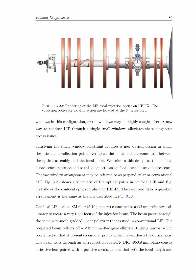
Plasma Diagnostics 86
Figure 3.22: Rendering of the LIF axial injection optics on HELIX. Thecollection optics for axial injection are located at the 6" cross port.
windows in this configuration, or the windows may be highly sought after. A new
way to conduct LIF through a single small windows alleviates these diagnostic
access issues.
Satisfying the single window constraint requires a new optical design in which
the inject and collection paths overlap at the focus and are concentric between
the optical assembly and the focal point. We refer to this design as the confocal
fluorescence telescope and to this diagnostic as confocal laser-induced fluorescence.
The two window arrangement may be referred to as perpendicular or conventional
LIF. Fig. 3.23 shows a schematic of the optical paths in confocal LIF and Fig.
3.24 shows the confocal optics in place on HELIX. The laser and data acquisition
arrangement is the same as the one described in Fig. 3.18.
Confocal LIF uses an SM fiber (5-10 µm core) connected to a ?2 mm reflective col-
limator to create a very tight focus of the injection beam. The beam passes through
the same wire-mesh gridded linear polarizer that is used in conventional LIF. The
polarized beam reflects off a ?12.7 mm 45-degree elliptical turning mirror, which
is oriented so that it presents a circular profile when viewed down the optical axis.
The beam exits through an anti-reflection coated N-BK7 ?50.8 mm plano-convex
objective lens paired with a positive meniscus lens that sets the focal length and

Plasma Diagnostics 87
Figure 3.23: A schematic of the confocal optical assembly with coordinatedirections marked. Red lines show the path of the injection laser. Blue linesshow the path of the collection optics. FP – multimode fiber port, L1 – f = 25mm plano-convex lens, PH – pinhole, L2 – f = 75 mm plano-convex lens, L3 –f = -50 mm plano-concave, L4 – f = 300 mm plano-convex lens, COL –reflective collimator, POL – wire grid linear polarizer, MIR – 45� ellipticalmirror, OBJ – plano-convex/meniscus objective doublet, FOC – sharedinjection/collection focus.
Figure 3.24: A top-down view rendering of the confocal optical assemblydeployed on HELIX.
therefore the sample volume location of the diagnostic. This doublet mitigates
chromatic and spherical aberration. When used on HELIX, the two lenses have a
measured combined focal length f = 149 mm. The polarization of the injection
beam is confirmed by placing a second linear polarizer in the optical path. The
transmitted power when the two polarization axes are normal is observed to be
⌧ 1% of the maximum when they are parallel, confirming that the polarization
has been preserved by the elliptical mirror and objective optics.
A subsection of the solid angle of the fluorescence passes back through the optical
assembly. A series of lenses reduces the diameter of the ray bundle and focuses
the collected light onto a pinhole spatial filter at the back of the optical assembly.
The pinhole size may be optimized for depth of field and diffraction-limited use,

Plasma Diagnostics 88
which suggests a smaller diameter should be used [149]. That said, a ?50 µm is
found to provide excellent depth of field and throughput for our needs. The light
exiting the pinhole is condensed by a final lens onto the orifice of an NA = 0.22,
?200 µm core multimode fiber, that transmits it to the PMT.
Absolute and relative density measurements require consistency in the diagnostic
between IVDFs recorded at different positions so that only the plasma influences
the result. Beside the consistently overlapping injection and collection focus, sev-
eral factors contribute to variations in intensity. The PMT bias and the settings
of the lock-in amplifier remain unchanged through the measurements. The wave-
length dependent transmittance variation of N-BK7 and the anti-reflective coating
during the laser sweep is estimated to be �T < 0.005% and is neglected. The laser
power also varies slightly with wavelength. For single-photon LIF the integrated
spectrum should increase linearly with increasing laser power, before plateauing
when the absorption saturates. For the plasma conditions in which the confocal
LIF data were recorded, the linear dependence is observed, and no plateau is seen
even at the highest power output of the laser.
An example IVDF, measured confocally in a 3.5 mTorr, 650 W helicon plasma
with B = 600 G, is shown in Fig. 3.17 with its reference iodine spectrum. The
IVDF indicates an essentially unmoving mean flow and ion temperature Ti = 0.24
eV. The SNR of this IVDF — µsig/�nse, the ratio of the signal average to the
standard deviation of the noise — is calculated to be approximately 15. The SNR
for conventional LIF under the same conditions is 22, indicating that at least 70%
of the conventional SNR can be obtained by the confocal technique.
Temperature and flow profile comparisons are shown in Fig. 3.25. The horizontal
error reflects the 0.5 mm uncertainty in the linear scale position used to identify the
position of the focus. The vertical error derives from error in the Maxwellian fit to
the IVDF and from shot noise. In the central region of the plasma, uconf. = 21±53
m/s, uconv. = �21± 41 m/s, T conf.i = 0.26± 0.05 eV and T
conv.i = 0.23± 0.03 eV,
confirming that conventional and confocal LIF produce comparable results.

Plasma Diagnostics 89
Figure 3.25: Temperature (a) and mean flow speed (b) profiles measuredwith conventional and confocal LIF.
The focal point and sample volume of the confocal optical arrangement is de-
termined by taking profiles of the injection and backlit collection optics using a
Newport LBP HR beam profiler. The beam profiler is a 7.6 mm x 6.2 mm active
area charge-coupled device (CCD) with 4.65 µm x 4.65 µm pixels. Imaging the
shape of the ray bundle for each optical path provides the location and distance
to the overlap region of the two bundles. Fig. 3.26 shows a series of beam profiles
showing the shape, focus and overlap of the injection and collection volumes sev-
eral millimeters around the focal plane. Negative distances correspond to planes
between the optics and the focal plane. Away from the focal plane, the elliptical
mirror creates a central obscuration that causes the collection ray bundle profile
to form an annulus whose radius decreases toward the focus. In a finite region
around the focal plane, the collection and injection ray bundles overlap. It is from
this region that the collected LIF signal originates. The optical response of the

Plasma Diagnostics 90
confocal LIF technique describes the spatial distribution of the light that con-
tributes to the signal for a flat density. The width of this optical response provides
a measure of how well the confocal optics isolate signal from the intended sample
volume and exclude signal from elsewhere. At f = 149 mm, this optical response
has a FWHM of 1.4 mm, from which 65.8% of the signal originates. This width
is about 30% broader than conventional LIF, which has a FWHM of 1.1 mm and
encompasses 97.3% of the signal. Previously published state-of-the-art for confocal
LIF exhibit collection regions several centimeters wide, leading to flattened pro-
files of measured plasma quantities [150]. By comparison, the excellent agreement
between the profiles measured confocally and in the conventional way, even on the
far side of the core at x > 0 as shown in Fig. 3.27, demonstrates that the spatial
localization of the two methods is similar.
Figure 3.26: Beam profiles showing the shape, focus and overlap of theinjection and collection ray bundles.
Figure 3.27: Relative metastable density profiles comparing the resolution ofconfocal and conventional LIF. PRF = 650 W, B = 600 G, n ⇡ 5⇥ 1018 m�3,Te ⇡ 3 eV.

Plasma Diagnostics 91
3.3.6 Ar-I LIF
Published LIF schemes for measuring neutral argon velocity distribution functions
(NVDFs) have existed since the mid-1980s [151]. They were developed further in
the subsequent decades to access multiple transitions and observe multiple direc-
tions simultaneously [152–154]. Ar-I LIF with diode lasers was demonstrated in the
early 2000s [144] and was combined with a collisional-radiative model to extract
absolute densities [81]. In the scheme employed in Refs. [144] & [81], the laser scans
over the 667.9125 nm resonance to pump the 4s(2P 03/2)1 non-metastable state to
the 4p0(2P 01/2)0 state, which decays to the 4s0(2P 0
1/2)1 state by emitting a 750.5934
nm photon. In Paschen notation this is the 1s4 ! 2p1 ! 1s2 excitation-decay tran-
sition sequence. While this pump transition is accessible through several available
dye and diode lasers, it has the disadvantage of requiring a sufficient population in
the non-metastable 1s4 state, which is primarily populated by the electron-impact
excitation of atoms occupying the nearby 1s5 and 1s3 metastable states. Recently,
a new 1s2 Ar-I LIF scheme demonstrated improved signal-to-noise over previous
approaches that pumps the 1s4 state by taking advantage of the improved sen-
sitivity photomultiplier detectors have to the visible range of the 706.9167 nm
2p3 ! 1s5 fluorescence [155]. In Ref. [154], the metastable 1s5 state is pumped
directly. However, this is accomplished by exciting to the 3p2 state through the
resonance at 395 nm, beyond the range of the Toptica DL100 and the Sirah Ma-
tisse DR with Rhodamine and Pyridine 1 dye [154]. The relative densities of 1s5
state in an inductive plasma has been studied in comparison to the other first level
Ar-I excitations (1s4, 1s3, and 1s2) in further detail in Ref. [153] and was observed
to exceed the densities of the other states by an order of magnitude.
For these experiments, we explored three schemes that take advantage of the highly
populated 1s5 metastable state and the high output power of the Sirah Matisse
dye ring laser. Fig. 3.28 shows a Grotrian energy level diagram of the pump and
fluorescence sequences used for probing the 1s4 and 1s5 states. In these schemes,
the metastable 4s(2P 03/2)2 (1s5) state is pumped to one of the states 4p0(2P 0
1/2)1,
4p0(2P 03/2)2, and 4p0(2P 0
3/2)1 (2p2, 2p3, and 2p4, respectively). These transitions

Plasma Diagnostics 92
Upper state �12 [nm] Decay state �23 [nm]4p0[2P 0
1/2]1 (2p2) 696.73524s[2P 0
3/2]1 (1s4) 727.49404s0[2P 0
1/2]0 (1s3) 772.63334s0[2P 0
1/2]1 (1s2) 826.67944p0[2P 0
3/2]2 (2p3) 706.91674s0[2P 0
1/2]0 (1s3) 795.03624s0[2P 0
1/2]1 (1s2) 852.37834p0[2P 0
3/2]1 (2p4) 714.90124s[2P 0
3/2]1 (1s4) 738.60144s0[2P 0
1/2]1 (1s2) 841.0521
Table 3.6: Summary of Ar-I metastable 4s[2P 03/2]2 (1s5) LIF schemes with
VIS/NIR transitions. Fluorescence lines observed are set in bold.
occur at 696.7352 nm, 706.9167 nm, and 714.9012 nm. The upper states have
several decay paths, all of which occur in the red to near infrared wavelength
range. The details of these transitions are shown in table 3.6.
Where the Ar-II and Ar-I (1s4) fluorescence is filtered by passing through a film-
based optical bandpass, the 1s5 fluorescence is passed through a McPherson Model
209 1.33 m Czerny-Turner high resolution monochrometer. The monochrometer
acts as a filter with a ±5 nm pass band [156]. During initial setup, light from a
NIST standard lamp transmits through an optical fiber onto the entrance slit of
the spectrometer. A CCD records a component of the dispersed spectrum around
the fluorescence wavelength. Once this wavelength is centered on the camera, the
standard lamp is exchanged for the fluorescence from the plasma, and a mirror
in the spectrometer cavity is turned so that the light reflects instead into an IR
sensitive PMT. The PMT signal passes to the lock-in amplifier and is recorded to
the lab computer.
Typical Ar-I spectra recorded in an inductive plasma — B = 450 G, Prf = 400 W, p
= 6 mTorr — with injection perpendicular to the magnetic field are shown in Fig.
3.29. Assuming a single neutral temperature and fitting these data to Eq. (3.44),
the three schemes produce significantly different temperatures: Tn = 0.027 eV for
the 2p2 scheme at 696.7352 nm, Tn = 0.038 eV for the 2p3 scheme at 706.9167 nm,
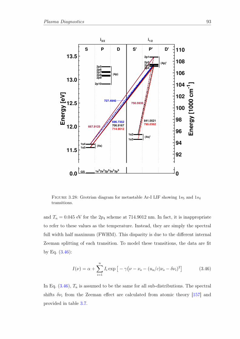
Plasma Diagnostics 93
0.0
11.5
12.0
12.5
13.0
13.5E
nerg
y [
eV
]
0
92
94
96
98
100
102
104
106
108
110
En
erg
y [
1000 c
m-1
]
S P D S' P' D'
j3/2
j1/2
1s5 1s4
1s3
1s2
2p10
2p9 2p8 2p7 2p6 2p5 2p4
2p3 2p2
2p1
GS 1s22s22p63s23p6
(4s)
(4s)'
(4p)
(4p)'
696.7352706.9167714.9012
667.9125
727.4940
841.0521795.0362
750.5935
Figure 3.28: Grotrian diagram for metastable Ar-I LIF showing 1s5 and 1s4transitions.
and Tn = 0.045 eV for the 2p4 scheme at 714.9012 nm. In fact, it is inappropriate
to refer to these values as the temperature. Instead, they are simply the spectral
full width half maximum (FWHM). This disparity is due to the different internal
Zeeman splitting of each transition. To model these transitions, the data are fit
by Eq. (3.46):
I(⌫) = ↵ +nX
i=1
Ii exp⇥� �
�⌫ � ⌫o � (un/c)⌫o � �⌫i)
2⇤
(3.46)
In Eq. (3.46), Tn is assumed to be the same for all sub-distributions. The spectral
shifts �⌫i from the Zeeman effect are calculated from atomic theory [157] and
provided in table 3.7.

Plasma Diagnostics 94
0.00
0.25
0.50
0.75
1.00
NV
DF
[a
.u.]
0.00
0.25
0.50
0.75
1.00
NV
DF
[a
.u.]
-1.5 -1.0 -0.5 0 0.5 1.0 1.5
Frequency ( -o) [GHz]
0.00
0.25
0.50
0.75
1.00
NV
DF
[a
.u.]
Data FWHM: 1.417 GHzData 'Tn': 0.045 eV
Model FWHM: 1.172 GHzModel 'Tn': 0.026 eV
Data FWHM: 1.433 GHzData 'Tn': 0.038 eV
Model FWHM: 1.185 GHzModel 'Tn': 0.026 eV
Data FWHM: 1.214 GHzData 'Tn': 0.027 eV
Model FWHM: 1.202 GHzModel 'Tn': 0.026 eV
Sch. 1 (696.7352 nm)
Sch. 2 (706.9167 nm)
Sch. 3 (714.9012 nm)
Figure 3.29: Example Ar-I 1s5 spectra recorded on-axis in an RF plasma: B= 450 G, Prf = 400 W, p = 6 mTorr, Plas = 3 mW. Modeling of the spectrausing theoretical Zeeman splitting provides an estimate of the neutraltemperature once Zeeman effects are removed.
The spectral widths of the sub-distributions now correspond to "temperatures"
that are similar: Tn = 0.026 eV for the 2p2 scheme at 696.7352 nm, Tn = 0.026
eV for the 2p3 scheme at 706.9167 nm, and Tn = 0.026 eV for the 2p4 scheme
at 714.9012 nm. These numbers are within error for the measurement, which is

Plasma Diagnostics 95
Upper state �⌫i (⇡) FWHM, �⌫Z⇡ FWHM, �⌫Z�[GHz] [MHz/mT] [MHz/mT]
2p2 (696.7352 nm) 0, ±0.168 4 52p3 (706.9167 nm) ±0.1512, ±0.3023 21 122p4 (714.9012 nm) 0, ±0.4289 25 30
Table 3.7: Summary of Ar-I metastable 4s[2P 03/2]2 (1s5) Zeeman effect
details. Credit: Amy M. Keesee.
⇡ 0.002 eV. The disparity in spectral width is predicted at least qualitatively by
the FWHM predicted for the ⇡ transitions, �⌫Z⇡, shown in table 3.7, for which
�⌫Z⇡ (2p4) & �⌫Z⇡ (2p3) > 6�⌫Z⇡ (2p2). Therefore, Zeeman splitting is sufficient
to explain the different spectral width provided by Eqs. (3.44) and (3.46). The
2p2 transition spectral width hardly changes, while the spectral width of the 2p4
transition is reduced by almost a half.
In addition to Zeeman broadening, these transitions are affected by laser saturation
broadening, in which greater laser power does not result in greater signal [158].
This effect manifests as a laser power dependence of the spectral width, as shown in
Fig. 3.30. Spectral widths measured with the 2p2 and 2p3 transitions show strong
Figure 3.30: The spectral width measured by each transition depends on theinjected laser power. The 2p2 and 2p3 transitions are most affected. The 2p4transition is minimally affected by laser saturation, but shows strong Zeemanbroadening.
dependence on laser power. Temperatures recorded with these transitions are not
valid for laser powers above approximately 10 mW in the test plasmas of Fig. 3.30.
Since the saturation level is dependent on the density of the probed species, i.e.
on the 1s5 metastables, best practice is to select a laser power so that the spectral
width does not change with increasing laser power.

Plasma Diagnostics 96
The Zeeman splitting of the Ar-I metastable spectrum is slightly different between
the ⇡ transitions are forbidden quantum mechanically. The spectrum splits into
two clusters whose separation depends on the magnetic field. The dependence is
linear in B. Fig. 3.31 shows an example spectrum with the two �± clusters resolved.
The three transitions exhibit different dependence of the splitting on the magnetic
-4 -2 0 2 4Frequency ( -
o) [GHz]
0
0.2
0.4
0.6
0.8
1
Ar-
I (1
s5)
LIF
in
ten
sit
y [
a.u
.]
B = 40 mT; p = 6 mTorr; Prf
= 400 W; o = 696.7 nm
2Z = 1.71 GHz
Figure 3.31: Ar-I spectrum recorded parallel to the magnetic field, showing�± clusters. The separation between the two clusters provides an estimate ofthe magnetic field strength.
field, as described by their Lande factors. Still, any of the three transitions can
be used to determine the background magnetic field by measuring the separation
of the two clusters. The magnetic field dependence of the cluster separation half-
distance is shown in Fig. 3.32. This half-distance serves as the shift of the peak
away from the drift velocity, un, of the neutral population and appears as �⌫Z in
Eq. (3.44).
3.3.7 Ar-II LIF
The experiments reported here measure IVDFs using the scheme proposed by Hill
et al. in Ref. [159] and explored in detail by Boivin in Ref. [146]. Fig. 3.33 shows a
transition diagram for this sequence. The absorption resonance from the 3d0 2G9/2
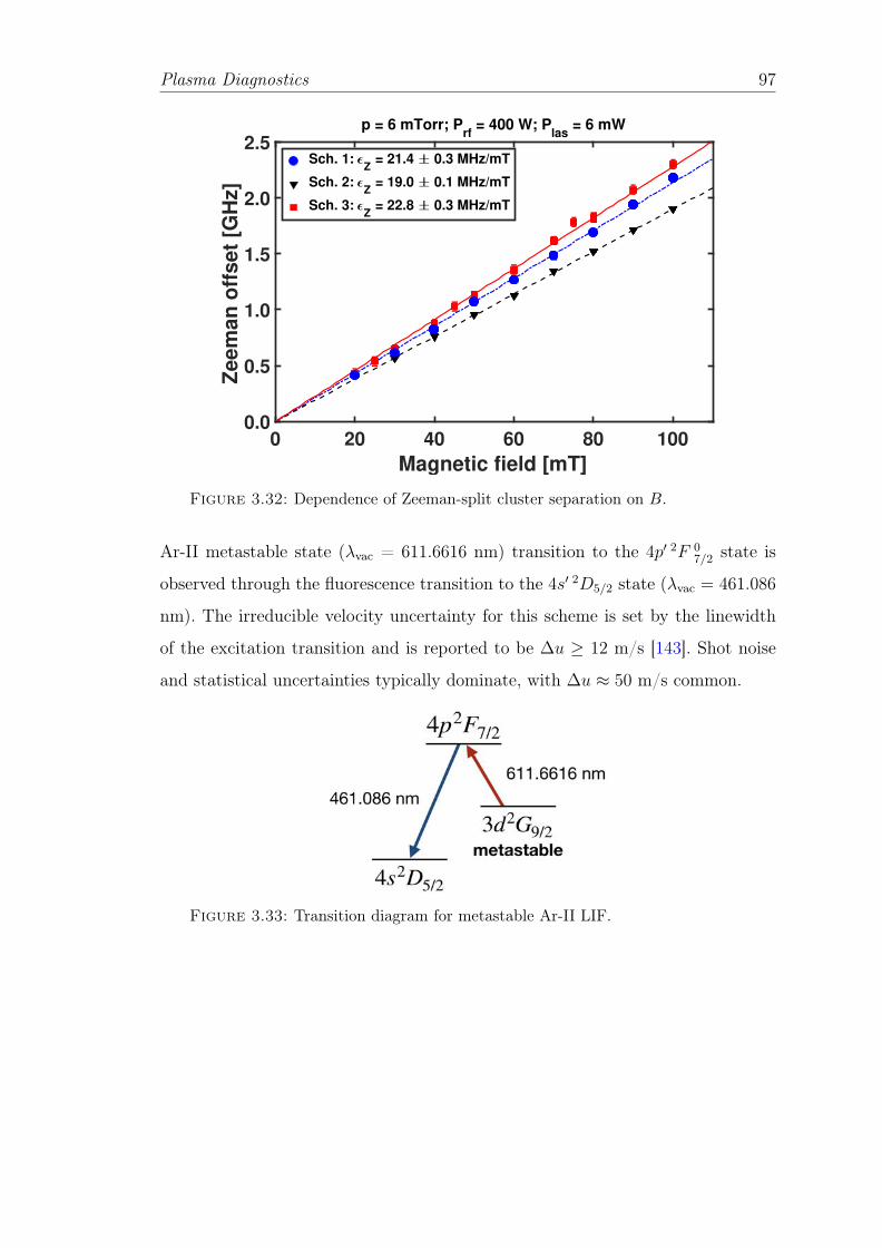
Plasma Diagnostics 97
0 20 40 60 80 100
Magnetic field [mT]
0.0
0.5
1.0
1.5
2.0
2.5
Ze
em
an
off
se
t [G
Hz]
p = 6 mTorr; Prf
= 400 W; Plas
= 6 mW
Sch. 1: Z = 21.4 0.3 MHz/mT
Sch. 2: Z = 19.0 0.1 MHz/mT
Sch. 3: Z = 22.8 0.3 MHz/mT
Figure 3.32: Dependence of Zeeman-split cluster separation on B.
Ar-II metastable state (�vac = 611.6616 nm) transition to the 4p0 2F 07/2 state is
observed through the fluorescence transition to the 4s0 2D5/2 state (�vac = 461.086
nm). The irreducible velocity uncertainty for this scheme is set by the linewidth
of the excitation transition and is reported to be �u � 12 m/s [143]. Shot noise
and statistical uncertainties typically dominate, with �u ⇡ 50 m/s common.
Figure 3.33: Transition diagram for metastable Ar-II LIF.

Plasma Diagnostics 98
3.3.8 Other considerations
Zeeman splitting and broadening effects
In the presence of an external field, Zeeman splitting occurs in which the degen-
eracy of each Ar-II energy level separates into several energy levels around the
unperturbed level. One group of these levels, for which the magnetic orbital quan-
tum number m doesn’t change during the transition (�m = 0) is referred to as the
⇡ transitions. Transitions for which �m = ±1 are referred to as �± transitions.
In LIF, these separated levels are convolved with the wider Doppler broadening of
the line and other broadening effects and create the appearance of multiple peaks
in the IVDF. If the field is insufficient to make the transition groups distinct, the
temperature is easily overestimated from the artificially broad IVDF.
When LIF is conducted with the laser passing across the magnetic field (i.e. for x
and y in boundary coordinates), the �± components are polarized perpendicular
to the field (� is shorthand for senkrecht, German for perpendicular). The laser
passes through a field-aligned linear polarizer, and the ⇡-polarized beam is not
resonant with the �-polarized transitions, eliminating the fluorescence from the
sixteen � (�m = ±1) components of the Zeeman-split spectrum.
When the laser is injected along the magnetic field, the �m = 0 transition is not
observed, and the �± transitions appear circularly polarized with opposite rotation
[160, pp. 243-248]. Since linearly polarized light contains both right- and left-hand
polarization components, unpolarized or linearly polarized light generates a bi-
modal fluorescence spectrum from the emission of the two � groups. Each peak is
shifted �⌫ = ±1.4 GHz/kG [144]. A �/4-plate placed after the linear polarizer,
oriented 45� to the polarization axis of the linear polarizer, causes the linearly
polarized laser to become circularly polarized. This circular polarization is resonant
with only one of the �± groups, selecting one of the peaks and eliminating the
fluorescence from the other. The mean speed of the IVDF is at the shift-corrected
location at the center of the bi-modal distribution.

Plasma Diagnostics 99
Several broadening mechanisms are present in each IVDF. In addition to splitting
the spectral lines, the Zeeman effect creates spectral broadening. For the plasma
conditions of these measurements, this broadening is estimated to be �Z⇡ ⇡ 1.8⇥
10�3 nm, < 4% of the ��D1/2⇡ 4.4⇥ 10�3 nm Doppler-broadening and is ignored
in the analysis. Stark broadening (O(10�6 nm)), line-width (O(10�5 nm)), power
broadening (< O(10�4 nm)) and pressure broadening (O(10�6 nm)) are negligible
for the Ar-II ions in these plasma conditions as well, contributing ⌧ 1% to the
broadening of the spectrum [145, 146]. Therefore, only Doppler broadening and
Zeeman effect shifts are incorporated into analysis of the LIF data.
One type of artificial broadening derives from instrumentation instead of from
atomic physics. The lock-in amplifier that the LIF signal passes through applies a
time averaging window to the signal. The VDF depends on the wavelength which
is swept over time, so an averaging window in time effectively applies a moving
average to the VDF in velocity, which for our sweep proceeds from negative to
positive velocities. The averaging window behaves as a low-pass filter. If the time
constant of the filter — i.e. of the averaging window — is small compared to the
scan time, the recorded VDF accurately reflects the VDF at the lock-in input,
before processing. If the window is large compared to the scan time, the VDF is
recorded in such a way that each point contains a significant contribution from
the portions earlier in time, or equivalently lower in frequency or velocity. A VDF
recorded in this way is shifted toward positive velocities. Fig. 3.34 illustrates this
effect by comparing a series of NVDFs measured at the same location, laser power,
and plasma conditions, but with different ratios of scan time to averaging window
width, in seconds. For time constants of one second, scan times 120 seconds and
longer produce an accurate, unshifted distribution. Shorter scan times introduce
a noticeable artificial shift toward positive velocities, up to several hundred m/s.
When the time constant is increased for noisy signals, the ratio between scan
time and time constant is kept constant for consistent flow measurements. Long
sweeps to mitigate overintegration easily enter the domain of diminishing returns,
opposing the researcher’s effort to make each measurement in the shortest time
possible without loss of accuracy. A method of selecting the scan time to time

Plasma Diagnostics 100
Figure 3.34: Example overintegration of VDFs.
constant ratio is demonstrated in Fig. 3.35. For a fixed time constant, the scan
time is increased until the mean flow speed levels off at some minimum value. The
scan time is selected that is shortest while not exceeding one standard deviation
from the measurement of the minimum speed. For the data in Figs. 3.34 and 3.35,
recorded with a one second time constant, a scan time of 120 seconds is the shortest
sweep that produces a speed within a conservative 25 m/s of the mean velocity at
240 seconds.
Figure 3.35: Overintegration trend in mean velocity for scan time selection.The arrow marks 120 s, the selected scan time used to measure subsequentVDFs.

Plasma Diagnostics 101
Reflections
Occasionally, the LIF laser beam will reflect off a surface in a way that the reflection
has sufficient power to create a second peak in the spectrum. This second peak is
created by absorption of laser light appearing to arrive from the opposite direction
of the primary beam, so that its fluorescence appears to be mirrored on the opposite
side of zero velocity from the primary peak. If the beam doesn’t reflect exactly
180�, the fluorescence will be produced by the projection of the reflected light
along the primary beam direction. This results in a reflected component that is
broader than the primary peak.
Fig. 3.36 shows an example progression of the IVDF as the sample region ap-
proaches the boundary from top to bottom in the figure. dy is the distance from
the sample region to the boundary surface in the vertical direction. The IVDF far
from the plate at dy = 10 mm does not have a significant reflection signal. The
reflection signal increases as the sample region approaches the boundary surface,
becoming comparable in intensity to the IVDF at dy = 1 mm. The exception
is the measurement at dy = 5 mm, where the laser terminates on a razor blade
beam dump that strongly attenuates the reflected signal. The functional form for
measurements which include reflected signals is a modified version of Eq. (3.45):
I⇤LIF(v) = A+ Cinj exp
� (m/2kB)
(v � u)2
T
�+ Crefl exp
� (m/2kB)
(v + u)2
Drefl
�
(3.47)
A, Cinj, Crefl, u, T and Drefl are fit parameters and serve similar functions to their
counterparts in Eq. (3.45). The second Gaussian, which describes the reflected
signal, is expected to be centered at the negative velocity of the primary peak.
(The width of the reflected peak, Drefl, is not truly a temperature and is given this
less suggestive notation.)

Plasma Diagnostics 102
Figure 3.36: IVDF showing the effect and analysis of laser reflections. Redcurves depict reference iodine distribution. Dark blue dots depict argonmetastable LIF signal. In light blue: primary IVDF (solid), reflection (dots),combined (dash).
Power budget
The expected final transmission through an optical train is a useful figure of merit
when aligning the laser to optical fibers and injection optics. As a general rule, as
long as the laser is stable, more power is better as signal scales linearly with power
in unsaturated single-photon LIF. If P laso
is the power of the laser as it exits the
laser cavity, and Tc is the transmission coefficient of an optical component, c, the

Plasma Diagnostics 103
total power injected into the plasma Plas is
Plas = P
laso
Y
c
Tc (3.48)
A list of the optical components and their transmission coefficients is shown in Tab.
3.8. The mechanical chopper transmits with 50% cycle-averaged transmission, so
that a power reading downstream is observed to have half the power when the
mechanical chopper is rotating. The plasma, however, is exposed to instantaneous
laser power oscillating from 0% to full transmission.
As an example calculation, the Ar-II laser passes through the splitter, the optical
diode, across two mirrors, through a multimode fiber, reflects off another mirror,
through the linear polarizer, through a lens, and finally through the chamber
window. If the initial power is 1300 mW, the transmitted power is
Plas =
�0.90⇥ 0.80⇥ 0.95⇥ 0.95⇥ 0.80⇥ 0.95⇥ 0.80⇥ 0.95⇥ 0.95
�⇥ 1300 mW
= 464 mW (3.49)
This constitutes a 36% overall transmission for a multimode fiber. A similar calcu-
lation for a single-mode fiber with the linear polarizer, �/4-wave plate combination
gives an expected transmitted power of 114 mW, or 9% total transmittance. To
excellent approximation, these transmittances are constant over laser power and
can be applied directly to the exit power of the laser to determine the power ex-
pected at the final output of the injection optics. In this way the laser power can
be checked overall or observed after each optical component to reduce any sources
of power loss to a minimum.
Laser beam profiles
The collimators used for LIF injection create a Gaussian profile beam. The axial
injection beam diameter is smaller than the injection for perpendicular injection,
as detailed in Sec. 3.3.4. The intensity distributions in the profiles in Fig. 3.37
reveal the structure of the injected beam and the weighting of the emission due

Plasma Diagnostics 104
Component Transmission coefficent, Tc
90:10 beam splitter 0.90Optical diode 0.80Each lens or mirror 0.95MM fiber 0.80SM fiber 0.25Linear polarizer 0.80Lin. pol. + �/4-plate 0.60Clean chamber window 0.95
Table 3.8: Approximate transmission coefficients of elements in the LIFoptical train.
to the collection optics. These intensity distributions are important because the
Figure 3.37: Beam profiles for parallel and perpendicular LIF. LIFmeasurements record an intensity-weighted average over the beam spot. Beamprofiler records images with a 9.3 µm/pixel sensor. Only horizontal profiles andwidths are shown.
signal that is recorded depends not only on the state of the plasma, but also on
the structure of the injection beam and the collection region.
The emission collected by the PMT, fpmt(x,v), due to the ideal distribution
f(x,v), and the optical response function, P(x;x0), is
fpmt(x,v) =
Zf(x0
,v)P(x;x0)d3x0

Plasma Diagnostics 105
Response function w (13.5%, 1/e2) [mm] � [mm]Laser, ?Horizontal 3.829 0.957Vertical 3.934 0.258
Laser, kHorizontal 2.027 0.507Vertical 2.192 0.548
Collection focus (? & k)Horizontal 1.145 0.286Vertical 1.198 0.300
Table 3.9: Response function parameters measured by beam profiles of theinjected laser and backlit collection optics.
The optical response function, P(x;x0), is the product of the laser and collec-
tion optics response functions: P(x;x0) = Plas(x;x0)Pcoll(x;x0). Unless they are
observed to be otherwise, the response functions are given a Gaussian form:
Plas(x;x0) = Pl,o exp
�
(x0)2
2�2l
�(3.50a)
Pcoll(x;x0) = Pc,o exp
�
(x0)2
2�2c
�(3.50b)
The 13.5% level I/Io normalized intensity widths are given in Fig. 3.37. �l and
�c are calculated from fitting Eqs. (3.50) to the beam profiles. The results are
shown in Tab. 3.9. The calculated response functions are used in creating synthetic
diagnostics for comparing simulations to measurement, and simulated spectra are
compared to the normalized spectra fpmt/Pc,oPl,o.
One implication of these finite extent response functions is that gradients with
shorter scales than the overlap region will be misrepresented by the LIF data.
Boundary regions, and Debye sheaths especially, have steep gradients over 10s of
microns, and are far too small to be resolved by LIF on HELIX. LIF measure-
ments that overlap these regions therefore record an ensemble of sheath particles

Plasma Diagnostics 106
combined with particles outside the sheath, and the measured gradients appear
smoothed.

Chapter 4
Three-dimensional, multispecies
measurements in a boundary with
an oblique magnetic field: B = 600
G, = 74�
4.1 Introduction
Measurements were made of the ion and neutral velocity distribution functions
(I/NVDF) and the electron energy probability functions (EEPFs) in three di-
mensions in a plasma boundary with magnetic field magnitude B = 600 G and
magnetic angle = 74�. The introduction of the absorbing boundary caused the
plasma to reestablish an equilibrium that is shifted from the mechanical axis by
several centimeters, as shown in Fig. 4.1. Statements like "outer radii" refer to
plasma radius, not mechanical radius. Unless stated otherwise, data are presented
in the (x, y, z) simulation coordinate system, and z = 0 mm lies along the me-
chanical axis. When the (x⇤, y
⇤, z) laboratory coordinate system is used it will be
indicated.
107

Experiments in the vicinity of a magnetized boundary 108
Figure 4.1: Detail of the coordinate systems showing the plasma shift. The(x⇤, y⇤, z⇤) system is aligned to the chamber mechanical axis and the pointwhere it intersects the boundary surface. The un-starred system is aligned withthe boundary geometry, and z = z⇤, and the two are used interchangeably. Thefour corners of the experimental domain are provided in the (x⇤, y⇤, z⇤)system. The mechanical axis lies along z = z⇤ = 0 mm. The distance to thesurface, d, is not necessarily from the boundary center.
4.2 Magnetic field measurements
Hall effect and Langmuir probe measurements establish a background environment
for the the ion and neutral dynamics in the boundary region. The magnetic field
measurements, performed at atmosphere, with the stainless steel boundary in place
and aligned, are shown in Fig. 4.2. The magnetic field deviation from the mean
Figure 4.2: Percentage spatial variation in magnetic field: Bk = By⇤ = 591 G,with the field direction indicated in light blue in (a). The magnetic fielddeviation from the mean does not exceed ±1% within the experimentaldomain. The solid black bar across the bottom marks the location of thesurface. White dots mark the measurement locations. White regions otherwisemark regions where no measurements were taken. These regions are slightlyaccentuated in the near vicinity of the surface. The plate normal distance, d, isshown normalized to the ion gyroradius, ⇢i.
does not exceed ±1% within the experimental domain, with all measured axial

Experiments in the vicinity of a magnetized boundary 109
fields falling within the range By⇤ 2 [586, 597] G. The fields in the two directions
perpendicular to the chamber axis are within Bz 2 [5, 20] G and Bx⇤ 2 [25, 36] G
(. 6%) and are neglected.
In tandem with the boundary in/boundary out measurements shown in Fig. 2.7,
these measurements confirm that a) the boundary does not distort the magnetic
field structure by more than 1%, and b) the magnetic field is axial and within 1%
of B = 591 G throughout the entire experimental domain. To within very good
approximation, the magnetic field is linear, axial, uniform, and incident on the
boundary at = 74�. While care was taken to align the gaussmeter probe for
this measurement, the stalk of the probe is not rigid, and small angle variations
in orientation likely account for the majority of the spread in the magnitudes
reported. The remainder is spatial variation from discrete electromagnets. The
structure apparent in Fig. 4.2, where the field magnitude is highest at the top
corners and lowest at the lower center of domain, results from the spacing of the
electromagnets, but these variations are small.
4.3 EEPF, ne, Teff, and pe from Langmuir probe
measurements
The plasma electrons are assumed to be magnetized and follow the field lines. (This
assumption will be verified in Sec. 4.6.) Druyvesteyn analysis (see Sec. 3.2.3.3)
was employed throughout, because it does not require that the electrons possess
a Maxwellian energy distribution, and because it gave close results to the full,
Extended Druyvesteyn analysis in significantly less time. As discussed in Sec.
3.2.3.3, the relative electron, ion, and probe scales produce a density that is un-
derestimated (⇡ 20%), and a temperature that is slightly overestimated (⇡ 10%),
when Druyvesteyn analysis is employed.

Experiments in the vicinity of a magnetized boundary 110
4.3.1 Non-Maxwellian features are observed in EEPFs
The electron energy probability function (EEPF) is constructed from the second
derivative of the electron current. Fig. 4.3 shows examples of typical EEPFs ob-
served in the Langmuir probe data. The 0th and 1st moments of these EEPFs
Figure 4.3: EEPF dependence on plasma (a) radius and (b) axial location. In(a), the arrow marks the presence of an energetic population at large radii.
provide density and electron temperature, respectively (see Sec. 3.2.3.3). Non-
Maxwellian electron populations appear in the EEPFs. For example, the EEPF in
(a) contains an energetic electron distribution with a peak at approximately 18
eV. These EEPFs, plotted on the same scale, indicate a radial density gradient
directed toward �x⇤. That the gradient is not characterized by proximity to the
boundary surface is seen in part (b), which shows measurements at constant x⇤
but at several distances from the surface. At all three of these locations the EEPFs
contain non-Maxwellian, enhanced high-energy tails.
The first excited state of argon is 11.55 eV, and the first two ionization energies are
15.76 eV and 27.63 eV [161]. The bulk of the electrons in the EEPFs measured in the
boundary possess less energy than the first excitation energy; the tail populations
are responsible for ionization and excitation to states probed by laser-induced
fluorescence (LIF).

Experiments in the vicinity of a magnetized boundary 111
4.3.2 The helicon source creates a radial density gradient
For much of the boundary region the electron population is not Maxwellian, and
the energy moment formulation of the electron temperature is preferable. Lang-
muir probe measurements of the plasma density and electron temperature are
shown in 3D in Figs. 4.4. Several features emerge from these measurements. First,
Figure 4.4: ne(x) in the boundary region.
the plasma density has a distinctly radial structure, with the maximum densi-
ties observed at the top of the domain, near the brightest emission regions. The
minima are consistently observed at the largest radii in the domain. The range
of densities observed is approximately 8⇥ 1016 m�3 to 7⇥ 1017 m�3. The plasma
density decreases with distance to the boundary surface, however this gradient is
less pronounced. There may be a slight axial density gradient as well, directed
toward the antenna (�y⇤), however the approximately 15-20% decrease in density
with increasing y⇤ is on the order of the measurement uncertainty, which is esti-
mated to be 20%, optimistically, or 50% conservatively. Fig. 4.5 shows the mean
and peak density in each z plane. The mean density suggests a centrally peaked
profile, however there is a clear trend toward higher peak density at increasing z,
suggesting that the plasma core may be shifted a few millimeters in z from the
chamber mechanical axis. The experimental domain rests within the more gradual
density gradients slightly away from the high density core.

Experiments in the vicinity of a magnetized boundary 112
Figure 4.5: Electron density and temperature dependence on z. Uncertaintiesare �z = ±1 mm. �ne = ±20% and �Teff = ±10%. The dashed line indicatesthe mean and the shaded region indicates the range.
4.3.3 Teff distribution reflects high-energy electron popula-
tions
The electron temperatures are observed to be fairly uniform, especially at z = 0
mm, the center of the domain. Fig. 4.6 shows a heatmap of the effective elec-
tron temperature Teff = 2h"i/3 distribution in the boundary region. Two features
Figure 4.6: Teff(x) in the boundary region.
emerge. First, the temperature at z = 0 mm is slightly higher than at larger |z|.
This dependence can be seen in the Teff mean and range shown in Fig. 4.5. Teff
decreases with the distance of each of these planes to the plasma core and is con-
sistent with the cylindrical structure of the helicon plasma. The second feature
that arises is the spatial distribution of the non-Maxwellian features of the EEPFs
shown in Fig. 4.3. The high-energy content of the EEPFs increases with plasma ra-
dius as the density decreases, and the resulting high effective temperature appears
at the outermost radii (x⇤ & 5 mm) of the experimental domain in Fig. 4.6.

Experiments in the vicinity of a magnetized boundary 113
4.3.4 pe = nekBTe shows a radial helicon electron pressure
gradient
The spatially varying density and relatively uniform electron temperature lead to
an electron pressure, calculated by the ideal gas law, pe = nekBTe — ne is the
electron density, kB = 1.602⇥10�19 J/eV is the Boltzmann constant, and Te = Teff
is understood — that is largely determined by the structure of the density, as shown
in Figs. 4.7 and 4.8. The cylindrical geometry of the helicon plasma is evident
Figure 4.7: Spatial structure of the electron pressure, pe.
Figure 4.8: Electron and ion pressure dependence on z. The dashed lineindicates the mean and the shaded region indicates the range.
in the radial dependence of pe in these images, with the pressure decreasing for
increasing x⇤. pe decreases at larger |z| because those planes are slightly farther
from the high density core.

Experiments in the vicinity of a magnetized boundary 114
4.4 �p depends on proximity to the boundary sur-
face
The plasma potential, �p, from Langmuir probe analysis is unreliabledue to the
asymmetry of the system caused by the magnetic field and because the probe dis-
turbs the presheath [2, 26]. The second derivative of the probe current provides a
guideline for �p, however it is expected to underestimate the actual potential by
O(10�1Te) (see Sec. 3.2.3.3). �p is shown in Fig. 4.9. Unlike ne and Te, �p is orga-
Figure 4.9: �p(x) in the boundary region.
nized in relation to the distance from the boundary surface, instead of in relation
to plasma radius. This behavior has been observed in unmagnetized sheaths at
absorbing boundaries [2] and isn’t surprising here. Variations across z are within
the measurement uncertainty of ��p ⇡ 0.5 V. The electric field associated with this
gradient accelerates the ions toward the boundary surface, diverting them from
their trajectories along the field lines. This field is also responsible for generating
any E⇥B drifts along the boundary.
4.5 Ion temperature and pressure, Ti(x,v) and pi(x,v),
distributions from LIF data
4.5.1 Ti is slightly anisotropic
The ion temperature, Ti, is measured from the width of the LIF spectrum, as
described in Sec. 3.3.2. LIF resolves the ion temperature, Ti, separately in every
injection direction. In this instance Ti,y⇤ = Ti,k, and Ti,x⇤ and Ti,z are perpendicular

Experiments in the vicinity of a magnetized boundary 115
to the applied field. The mean temperature over all three directions is 0.35 eV with
a standard deviation of 0.05 eV. Ti(x,v⇤) is shown in Fig. 4.10, each row of which
shows the temperature along one lab-frame direction.
Figure 4.10: Ti(x,v⇤) in 3D3V. Ti,x⇤ , shown in (a)-(e) represents one of thetemperature components perpendicular to the magnetic field. The temperatureparallel to the magnetic field, Ti,y⇤ = Ti,k, is shown in (f)-(j). The secondperpendicular direction, Ti,z⇤ , is shown in (k)-(o). As before, each columnrepresents one planar location in z. The hot spot on the downstream (left) sideof (k)-(o) is an artifact from laser reflections. Blue patches in (b)-(d) and(g)-(i) mark the extent of the laser beam dump (BD) in each plane. For themeasurements in (k)-(o), the laser passes across the boundary surface and doesnot contact the beam dump.
Ti,x⇤ increases by 0.05 eV from the upstream to the downstream edge of the
domain. The ions in this direction cool slightly just above the surface. At z < 0
mm, there is a thin layer of ion heating where temperatures 0.09 eV above the mean
are observed just above the cool region at the boundary surface. Measurements
in this direction suffer from distortion due to laser reflections of the boundary
surface. A circular laser beam dump at the center of the boundary, marked by
blue patches in (b)-(d) and (g)-(i), mark the extent of the laser beam dump in
each plane. This beam dump substantially, but not entirely, reduces the amount
of reflected signal in the LIF spectrum (see "Reflections" in Sec. 3.3.8). The drop
in temperature may be a result of an inaccurate reflected signal fitting algorithm,
however it is significant that the measurements taken when the laser is incident
on the beam dump show temperatures that are comparable to the measurements

Experiments in the vicinity of a magnetized boundary 116
when the laser is not. The same fitting algorithm — identify the LIF signal in
the injection direction with mean flow u, look for a second peak at �u but with
arbitrary temperature, then fit for u and Ti — is applied over the entire domain.
Far from the surface, this algorithm finds a reflected signal contribution <1%.
Ti,z increases from 0.26 eV, at the upstream entrance to the domain on the right
side of (k)-(o) of Fig. 4.10, to approximately 0.40 eV near the wall downstream
(left). There is an axial gradient apparent in the data, with a slight increase in
Ti,z just above the surface. The hot spot on the downstream side of (k)-(o) is an
artifact from laser reflections and does not represent the true temperature of the
ions there.
Parallel to the magnetic field, Ti,y⇤ increases approximately 0.05 eV between the
upstream and downstream edges of the domain. Temperature gradients with re-
spect to the distance from the surface are inconsistent across z. Temperatures in
this direction are slightly higher, with mean temperature Ti,y⇤ = 0.39 eV, compared
to Ti,x⇤ = 0.36 eV and Ti,z = 0.33 eV. The temperature measurement uncertainty
�Ti arises from systematic errors in the technique and from statistical variation in
identical measurements. �Ti(syst.) = ±0.012 eV, and the statistical uncertainties
calculated from fiducial measurements are shown in Tab. 4.1. The temperature
anisotropy is therefore greater than the uncertainty in the measurement. A higher
axial temperature is consistent with the presumed greater diffusivity of ions along
the field lines compared to cross-field transport. Preferential acceleration along
the boundary electric field and subsequent thermalization causes the disparity
that Ti,x⇤ 6= Ti,z, even though these temperatures both describe the motion of
particles across field lines.
4.5.2 The ion pressure is isotropic: pi(x,v) ⇡ pi(x)
The ion temperatures in Fig. 4.10 are used to construct the ion pressure in 3D3V,
which is shown in Fig. 4.11. In this figure, the directional ion pressures are calcu-
lated from pi,x⇤ = nikBTi,x⇤ , pi,y⇤ = nikBTi,y⇤ , and pi,z⇤ = nikBTi,z⇤ . The pressures

Experiments in the vicinity of a magnetized boundary 117
Component �Ti [eV] IVDFs contributing, #
Ti,x⇤ 0.010 2291-2295
Ti,y⇤ 0.011 2743-2747
Ti,z 0.015 3297-3300, 3396, 3397, 35753576, 3666, 3667, 3760, 3761
Table 4.1: Statistical uncertainty �Ti(syst.) calculated via repeated fiducialmeasurements. x⇤ = (�10,�30, 0) mm.
Figure 4.11: Spatial variation of pi(x,v). Bright regions at extreme left in(k)-(o) are an artifact of laser reflections
are remarkably similar in all three directions, such that pi(x,v) ⇡ pi(x), again
driven by the density variation and the relative uniformity of Ti. The radial gra-
dient appears in all three directions as it did for the electrons, and it is difficult
to ascribe a gradient with respect to the boundary independent of the radial pres-
sure drop. It is significant that no strong pressure gradients along the axis are
observed, with the strongest observed at z = �10 mm, with point-to-point mag-
nitude �pi,x⇤/�y⇤ = 0.46 Pa/m. This corresponds to a pressure force on the ions
of order Fp
i⇠ 10�18 N directed downstream (assuming ni = 5 ⇥ 1017 m�3). The
mean of each z plane peaks at z = 0 mm, however the maximum pressure in each
plane increases with z (Fig. 4.8).

Experiments in the vicinity of a magnetized boundary 118
The pressure gradients in Fig. 4.11 suggest a possible explanation for the obser-
vation that Ti,x⇤ > Ti,z in Sec. 4.5.1: the ions experience an accelerating pressure
gradient in x⇤ that they do not experience in z. The electric field of the boundary
provides an additional accelerating force to the ions along the x⇤ and y⇤ directions.
The collisions in the presheath then thermalize the populations, producing higher
temperatures along the directions of acceleration. Upstream of the experimental
domain, 300 mm from the boundary, the axial ion temperature is Ti,y⇤ = 0.29±0.02
eV. By the time the ions enter the experimental domain Ti,y⇤ � 0.32 ± 0.02 eV,
which suggests additional forces contribute to ion acceleration and heating between
the antenna and the boundary region.
4.5.3 Characteristic velocities in the boundary
The electron and ion thermal speeds, and the sound speed in the boundary, are
calculated from the temperature data using the following relations:
vthe =p8Te/⇡me
vthi =pTi/mi
cs =p(Te + Ti)/mi.
The range and mean velocity in the boundary are shown in Tab. 4.2.
4.6 Characteristic frequencies in the boundary
The cyclotron frequency, !c = eB/m is calculated from the magnetic field mea-
surements, where B = 0.059 T, or 590 G. The plasma frequency, !p =pne2/m✏o,
is calculated from Langmuir probe densities. These quantities are shown in Tab.
4.3.
The characteristic collision frequencies are calculated using the measured plasma
quantities. The argon ions (Ar+), gas particles (Ar), and electrons (e�) undergo a

Experiments in the vicinity of a magnetized boundary 119
Velocity Minimum [m/s] Mean [m/s] Maximum [m/s]
vthe 1.13⇥ 106 1.32⇥ 106 1.56⇥ 106
vthi,x⇤ 700 910 1070
vthi,y⇤ 790 970 1160
vthi,z 760 890 1020
vthi (overall) 700 930 1160
cs 3000 3500 4090
Table 4.2: Characteristic velocities. vthi,z omits reflection artifacts. cs istabulated using all ion temperatures.
Frequency Minimum [rad/s] Mean [rad/s] Maximum [rad/s]
!ce 1.03⇥ 1010 1.04⇥ 1010 1.05⇥ 1010
!pe 1.35⇥ 1010 2.88⇥ 1010 4.81⇥ 1010
!ci 1.42⇥ 105 1.43⇥ 105 1.44⇥ 105
!pi 0.50⇥ 108 1.07⇥ 108 1.78⇥ 108
!RF - 5.97⇥ 107 -
Table 4.3: Plasma and cyclotron frequencies for both charged species. TheRF frequency, !RF, is included for comparison.
menagerie of collisions, even if impurity species from the air and chamber materials,
such as O2, N2, C and Fe, are neglected.
Several kinds of ion collisions are considered that fall into three broad categories:

Experiments in the vicinity of a magnetized boundary 120
ion-neutral elastic scattering, ion-neutral inelastic reactions, and Coulomb colli-
sions with electrons:
Ar + Ar+ �! Ar + Ar+ Elastic scattering (SC)
Ar + Ar+ �! Ar+ + Ar Charge exchange (CX)
Ar + e�
�! Ar+ + 2e� Ionization (IZ)
Ar+ + Ar+ �! Ar+ + Ar+ Coulomb scattering (II)
Ar+ + e�
�! Ar+ + e� Coulomb scattering (IE)
e� + Ar+ �! e
� + Ar+ Coulomb scattering (EI)
e� + e
��! e
� + e� Coulomb scattering (EE)
In elastic scattering collisions (SC), an argon ion and an argon neutral ballistically
scatter, exchanging momentum in the process. Charge exchange (CX) collisions
occur when a passing ion acquires an outer shell electron from a neutral atom.
This mechanism is important for momentum transfer, as it results in neutral par-
ticles impacting the boundary surface after having accelerated to high velocities as
ions. In a sense, the neutrals experience the fields in the boundary via this inter-
action. When it occurs, charge exchange appears in LIF spectra as a fast neutral
population and a corresponding depletion of energetic ions. Recombination has
a similar effect, in that it results in strong momentum transfer between the ion
and neutral populations. Ionization from electron impact is a source mechanism for
positively charge ions. Coulomb collisions (II, IE, EI, EE) are interactions between
the charged particles’ local fields in which the particles’ trajectories are redirected.
The frequencies of these collisions depend on the density of the target species and
on the ion energy dependent cross-section, �(E), of the interaction. The cross-
sections have been predicted theoretical, however given the complexity of the
problem, the experimental measurements should be used. Example elastic, ion-
ization, and excitation cross sections are shown in Fig. 4.12 from Refs. [162, 163].
An approximate form for �SC is given by [162, 164]

Experiments in the vicinity of a magnetized boundary 121
Figure 4.12: Experimental ion collision cross-sections [162, 163].
�SC(E)[m2] = 7.8⇥ 10�19� 2.0⇥ 10�19
p
E 0 E 4
= 2⇥ 10�19 + 5.5⇥ 10�19E
�1/2E � 4
however �SC and �CX are determined from the experimental data in Ref. [124],
which are reproduced in Fig. 4.13. A numerical fit to the CX data gives the relation
Figure 4.13: Experimental �CX and �SC, with ⌫CX and ⌫SC calculated for arange of neutral densities. Pale bars represent standard deviation in collisionfrequency from standard deviation in cross section. Lines represent the collisionfrequency calculated with the mean cross section.
�CX(E)[m2] = 1020⇥59.28� 3.257⇥ 10�4
E � 4.641 ln(0.35)⇤.

Experiments in the vicinity of a magnetized boundary 122
Estimates of collision frequencies from scattering and charge exchange interactions
are calculated by the relation
⌫ = nn�vth (4.1)
and require estimates of the neutral density, nn and the mean velocity, vth, of the
moving particles, for which the mean thermal speeds in Tab. 4.2 are used.
The ionization rate, KIZ, is approximated by the relation [121]
KIZ(Te)[m3/s] = 2.34⇥ 10�14T
0.59e
exp(�17.44/Te),
and shown over a range of Te in Fig. 4.14. The ionization frequency is calculated
Figure 4.14: Dependence of KIZ and ⌫IZ on nn and Te. The pale blue shadedregion marks range of measured electron temperatures.
by ⌫IZ = nnKIZ. (A full treatment of collisions requires integrating the collision
integral, however approximate solutions will be used here to determine scaling
instead of using the more involved analysis reserved for simulations.)
Fig. 4.14 demonstrates a major challenge of simulating low temperature plasma
boundaries: the neutral density can not be measured absolutely in pure argon and
is difficult to estimate, however the collisionality is often very sensitive to it. A
naive estimate of the neutral density of the gas interacting with the plasma is
obtained by the ideal gas law, nn = pn/kBTn, where pn = 3.6 mTorr (0.48 Pa) is

Experiments in the vicinity of a magnetized boundary 123
measured by the pressure gauges in the chamber wall, and the neutral temperature
Tn ⇡ 0.028 eV is measured by LIF. These conditions suggest nn = 1.07⇥1020 m�3.
This method assumes that the neutral profile is flat across the chamber, and that
there is no change in pressure between the location of the pressure gauge and the
experiment. Both assumptions are faulty. Measurements in HELIX have demon-
strated high ionization rates in the core of the helicon plasma, with corresponding
depletion of the neutral population [81]. In the CHEWIE device, experiments in
krypton show neutral density and profile shape dependence on magnetic field mag-
nitude, fill pressure, RF frequency, and RF power [85].
The radial neutral profile in HELIX was recently (Ref. [164]) estimated for several
plasma diameters using a method proposed by Gilland et al. [79]. The results are
shown in Fig. 4.15. According to these calculations, the neutral density along the
Figure 4.15: Neutral depletion on-axis in HELIX for several plasmadiameters [164].
axis is between 44% and 90% of the pressure measured at the edge. Profiles from
Keesee et al. [81], discussed in Sec. 1.3.4, suggest a comparable range, with some
authors claiming as much as a factor of 4 neutral depletion from maximum neutral
density [83]. This drastically changes the frequencies of collisions involving neutral
particles, which are at least linearly dependent on nn.

Experiments in the vicinity of a magnetized boundary 124
The cross sections, calculated from the data in Fig. 4.13, are �CX = 6.415⇥ 10�19
m2 and �SC = 8.5078⇥10�19 m2. Mean collision frequencies at 75% neutral fraction
are ⌫SC = 6.34 ⇥ 104 s�1 and ⌫CX = 4.79 ⇥ 104 s�1. (Ref. [164] calculates the full
collision integral, using 100% neutral density and a flat profile. Collision frequencies
calculated in this way are typically larger by a factor of about 2.)
Coulomb collisions depend on the Coulomb logarithm, � .= ln⇤, which describes
the ratio of the of the maximum and minimum applicable values of the impact pa-
rameter during a collision. It is different depending on the two particles interacting.
Detailed numerical approximations of the Coulomb logarithm from experimental
data are provided by the NRL Plasma Formulary [123], however in most cases
� ⇡ 10. When Time/mi < Te < 10 eV, for electron mass me = 9.11 ⇥ 10�31 kg,
argon ion mass mi = 6.6335⇥ 10�26 kg, and singly-ionized atomic argon:
�EE = 23.5� ln⇥(ne/10
6)1/2T�5/4e
⇤�
⇥10�5 + (lnTe � 2)2/16
⇤1/2
�EI = �IE = 23� ln⇥(ne/10
6)1/2T�3/2e
⇤
�II = 23� ln⇥(2ni)
1/2T
�3/2i
⇤
These quantities are shown as functions of Te, Ti and n in Fig. 4.16.
Figure 4.16: Dependence of ln� on Te, Ti and n.

Experiments in the vicinity of a magnetized boundary 125
The electron-electron, electron-ion, ion-electron, and ion-ion collision frequencies
are given by the Lenard-Balescu kernel:
⌫EE[s�1] ⇡nee
4
4⇡✏2om
1/2e T
3/2e
�EE(ne, Te) (4.2)
(4.3)
⌫EI[s�1] ⇡
p2
12⇡3/2
nie4
✏2om
1/2e (kBTe)3/2
�EI(ne, Te) (4.4)
(4.5)
⌫IE[s�1] ⇡ (me/mi)⌫EI (4.6)
(4.7)
⌫II[s�1] ⇡nie
4
12⇡3/2✏2om
1/2i
(kBTi)3/2�II(ni, Ti) (4.8)
from [123, p. 34], [165], and [166, p. 217], where permittivity of vacuum ✏o =
8.854 ⇥ 10�12 F/m. The Ti and Te dependence of these collision frequencies is
shown in Fig. 4.17.
Figure 4.17: Dependence of Coulomb collision frequencies on Te, Ti andne ⇡ ni. Pale blue regions mark the extent of Te and Ti observed.
Recent experiments by Yip et al. [167] and Claire et al. [23] have challenged the
assumption that ion-ion collisions are necessarily negligible in the presheath. In re-
sponse, Baalrud et al. have extended the traditional Lenard-Balescu theory in Eq.
(4.2) to include ion-acoustic and ion-ion two-stream instability enhanced collisions
[165]. They argue that these instabilities effectively thermalize non-Maxwellian

Experiments in the vicinity of a magnetized boundary 126
tails arising in IVDFs from ion-neutral collisions. The authors were not consider-
ing plasmas in significant magnetic fields, however they propose a parameter
⌘.=�ps
�De
r⇡me
16mi
which determines the size of the electron-electron collisional enhancement, as the
enhanced collision frequency ⌫⇤EE / exp(⌘x/�ps). �De is the electron Debye length
�De =
s✏okB/e
2
ne/Te + ni/Ti
,
and �ps is the presheath scale length, which is estimated by the the ion-neutral
collision length �IN = vthi/⌫IN. For all but the most extreme plasma parameters
observed, ⌘ . 0.83, and on average ⌘ ⇡ 0.12, indicating that instabilities do not
contribute to IVDF thermalization in a significant way. In the MARIA experiment
[21], however, at lower , the presheath scale was 3-4 times larger, and instability
enhanced collisions may have occurred in those boundaries.
The collision frequencies are summarized in Tab. 4.4, with total ion-neutral col-
lision frequency ⌫IN = ⌫CX + ⌫SC, total ion collision frequency ⌫I = ⌫IN + ⌫II + ⌫IE,
and total electron collision frequency ⌫E = ⌫IZ + ⌫EI + ⌫EE. Ion-neutral collisions
are expected to be comparable to ion-ion collisions and dominate ionization.
The influence of the magnetic field depends on the collisions the particles make
while traveling along field lines. If the particles experience no collisions, they follow
field lines closely with little transport across them. These particles are referred to
as "magnetized." At the other extreme, particles that undergo many collisions per
gyration do not travel along any one field line for very long before transferring
to the next, and the magnetic field does not tightly define the structure of the
motion of these particles. These particles are referred to as "unmagnetized" or
"collisional." The quantity that determines the collisionality regime of each species
is called the Hall parameter, the ratio of gyrofrequency to collision frequency, !c⌧ ,
where ⌧ = ⌫�1. (It is convention to compare frequencies in this way, even if the
resulting units are radians.) When !c⌧ � 1, the particles follow the field lines

Experiments in the vicinity of a magnetized boundary 127
Frequency Minimum [s�1] Mean [s�1] Maximum [s�1]
⌫SC 2.10⇥ 104 6.34⇥ 104 8.47⇥ 104
⌫CX 1.20⇥ 104 4.79⇥ 104 7.96⇥ 104
⌫IZ 2.50⇥ 103 4.92⇥ 104 2.80⇥ 105
⌫II 1.19⇥ 105 3.3⇥ 105 7.4⇥ 105
⌫IE 2.4 17 66
⌫EI 1.70⇥ 105 1.3⇥ 106 4.8⇥ 106
⌫EE 4.90⇥ 104 4.0⇥ 105 1.7⇥ 106
⌫IN 3.3⇥ 104 1.11⇥ 105 1.64⇥ 105
⌫I 1.52⇥ 105 4.41⇥ 105 9.14⇥ 105
⌫E 2.22⇥ 105 1.75⇥ 106 6.78⇥ 106
Table 4.4: Collision frequencies for measured range of Te, Ti, and n. Min.,mean, and max. n: 5.7⇥ 1016 m�3, 2.8⇥ 1017 m�3, 7.3⇥ 1017 m�3. Min.,mean, and max. Te: 2.84 eV, 3.92 eV, 5.46 eV. Min., mean, and max. Ti: 0.20eV, 0.36 eV, 0.56 eV. For collisions with neutrals, the minimum is calculatedusing 20% and the mean is calculated using 75%. Assuming a flat profile and0% ionization, nn = 1.07⇥ 1020 m�3.
closely and the background field strongly determines the structure of the plasma
and its flows. When !c⌧ ⌧ 1, collisions disrupt this organization and particles
easily diffuse across field lines.
The ions have a Hall parameter of !ci⌧i = 0.5 ± 0.3, indicating an intermediate
regime. The magnetic field plays an important, but not dominant, role in deter-
mining the behavior of the ions. The range given for !ci⌧i arises from reasonable
assumptions about the range nn and � may take. (Author note: Although this
number arises from discussions with Dr. Rinat Khaziev of Ref. [164], fault for any
error in it remains with me.) The Hall parameter for the electrons indicates clear
magnetization: !ce⌧e � 1500.

Experiments in the vicinity of a magnetized boundary 128
4.7 The metastable Ar-II drift velocities measured
by LIF show a 3D flow field
The primary aim of LIF measurements in the plasma boundary is to observe ion
flows and the potential interaction of ion and neutral species. Ion flow fields are
constructed from the 1st velocity moment of the distribution function, which for
Maxwellian distributions occurs at the peak of the distribution. The velocities are
measured in the laboratory system (x⇤, y
⇤, z) before being rotated into the (x, y,
z) simulation coordinate system (see Sec. ). The (ux, uy, uz) velocities, normalized
to the local sound speed, cs(x), are shown in Fig. 4.18. This data set contains the
Figure 4.18: 3D map of Ar-II metastable drift velocities from LIF data.Flows are presented in the simulation frame (ux, uy, uz) and normalized to thelocal sound speed. Dark regions at the downstream end of graphs (k)-(o) areartifacts from laser reflections and do not represent actual velocities.
only known 3D measurement of ion flows in a boundary region, the only known
measurements in the uz direction, and the only known ion flow measurements of
the boundary region at � 60�.
300 mm upstream of the boundary, at the chamber mechanical axis, the drift
velocity measured parallel to the magnetic field is uk = 110± 35 m/s. Normalized
to the mean sound speed in the boundary (cs = 3500 m/s), this corresponds to
parallel Mach number uk/cs ⇡ 0.03. From this initial velocity, the ions accelerate
to uk/cs � 0.41 at the upstream entrance to the boundary domain. Upon entering

Experiments in the vicinity of a magnetized boundary 129
the domain, uy/cs — which is at a small angle to uy⇤/cs = uk/cs — does not
significantly accelerate.
The ion drift velocities increase substantially in the direction normal to the bound-
ary. With the addition of this drift, the ion motion is at least two-dimensional.
From ux/cs � 0.16 at the boundary entrance, the ions accelerate along �@�p/@x
up to ux/cs = 0.78 just above the surface. The Bohm criterion, wherein ux � cs at
the sheath edge, is never observed. This is at least in part due to a large LIF sam-
ple region with respect to the size of the sheath. In Sec. 3.2.3.3, the Debye length
was calculated to be 0.03 - 0.05 mm, and a conservative estimate for the sheath
width is max(he, hi) ⇡ 0.6 mm. The effective collection volume for the transformed
velocities is at least 1.2 mm. Any measurement of the sheath therefore necessarily
measures a substantial ion population outside the Debye sheath, and the weighted
average is observed in the LIF spectrum. This deflection from field-parallel to drift
toward the boundary was observed by Siddiqui et al. [21] at 60�. These data
confirm that the deflection phenomenon occurs to 74�.
These two drift components exist in the E�B plane. As shown in (k)-(o) of Fig.
4.18, the ion drift acquires a third, non-linear component and diverts from uk not
only along x, but in the direction parallel to E⇥B as well. The presence of these
drifts was predicted in fluid theory boundary models by Reimann [168], Ahedo [10]
and others, and was required by Siddiqui et al. to match fluid models to the 2D
data in their experiments [21]. The ion drifts observed along z constitute direct,
non-perturbative measurements of ion transport across field lines in a boundary
with an oblique magnetic field. In addition, for uz(z 0), the ions flow against
the pressure gradient @pi/@z seen in Figs. 4.11 and 4.8.
Drift in the E⇥B direction is not due solely to the rotation of the plasma column.
The acceleration of the ions clearly depends on their proximity to the boundary
surface and not on plasma radius. At the top of the experimental domain, where
d/⇢i = 3.8, uz/cs < 0.01. uz/cs increases linearly to a maximum of uz/cs =
0.18� 0.20 between d/⇢i = 0.5� 0.7.

Experiments in the vicinity of a magnetized boundary 130
Within d/⇢i . 0.5, uz/cs surprisingly decreases to 0.1. The cause of this decrease
is not known. It is unlikely to be a reflection effect from laser bombardment of the
mounting flange, which is 50 cm away, since the return beam would be diffuse.
In addition, the flange is covered by a large area razor blade beam dump that
strongly attenuates the reflected beam. It is unlikely caused by a large sample
volume, since the drift velocities begin to decrease more than one laser diameter
away from the surface. It is also not a consequence of the interpolation algorithm;
the original data is shown in Fig. 4.19. The phenomenon occurs at the velocity
Figure 4.19: Data showing decrease in uz near boundary before interpolation.
distribution level. Fig. 4.20 shows the vz velocity distributions, normalized to the
maximum signal of the set, recorded at different distances to the boundary surface.
These measurements reveal shifted Maxwellian distributions that slow within a few
Figure 4.20: vz distribution function cascade with distance to the boundarysurface.
tenths of a gyroradius from the surface. The effects of inelastic collisions like charge
exchange and ionization do not appear in the Maxwellian vz distributions like the
ones shown in Fig. 4.20, however they are expected to be small and are likely
unresolvable. The upper bound on any divergence from a Maxwellian-distributed
population is 2%.

Experiments in the vicinity of a magnetized boundary 131
4.8 Testing Chodura’s model
As discussed in Sec. 1.1.1, the Bohm-Chodura criterion predicts that ux/cs � cos
occurs a distance �mps =p6(cs/!ci) sin from the Debye sheath edge. Siddiqui
et al. conducted a series of experiments in the MARIA device in the vicinity of
a boundary arranged at several angles to the magnetic field. LIF measurements
were taken of the ion flow to the boundary in two dimensions. Fig. 4.21 shows a
comparison between these measurements and Chodura’s prediction for the length
of the magnetic presheath [22]. The data from the MARIA experiments clearly
Figure 4.21: Comparison between ui measurements in MARIA andChodura’s prediction [22]. Blue arrows show 2D ion velocities. White ovalshows the location of Chodura’s prediction for the location where uk = cs. Redovals show the location measured by Siddiqui.
show that for every 60� the Bohm-Chodura criterion is met closer to the
boundary than Chodura proposed. In other words, the ions are drifting more
slowly than predicted. The predicted and observed locations of the Bohm-Chodura
criterion in the HELIX measurements is shown in Fig. 4.22. The Chodura model
is intended for plasma boundaries in which �i/⇢i � 1, which is not the case in
the HELIX experiments, and therefore is expected to be a poor description of the
boundary structure. That said, these measurements corroborate the observations
of Siddiqui et al. [21], which span �i/⇢i = 0.5 � 4 in finding that the predicted
distance of the magnetic presheath edge is typically farther from the wall than
observed, by a factor of about 4 in HELIX, and extend them to = 74�.

Experiments in the vicinity of a magnetized boundary 132
Figure 4.22: (Left) Comparison of predicted and observed �mps. (Right)Profile of observed �mps/⇢i. The dashed line indicates the mean and theshaded region indicates the range.
Combined 3D LIF and probe data allow the Chodura model to be investigated at
multiple locations in z along the boundary. Figs. 4.23 and 4.24 show the location
of the Chodura boundary in 3D. The criterion is satisfied at different locations for
different locations in z. The z dependence of �mps is shown at right in Fig. 4.22.
The asymmetry of the observed �mps is a surprising feature in these data, since
the z dependence of the other observed variables is either flat or symmetric about
z = 0 mm. Observed �mps ranges from 6.1 mm (⇢i) to 13.2 mm (2.1⇢i), with an
average distance of 9.3 mm (1.5⇢i). Siddiqui et al. found that at = 60�, the
Chodura criterion is predicted to be met at �mps/⇢i = 6.3, whereas they observed
it occur at �mps/⇢i = 0.6±0.01 [21]. It is worth noting that Chodura, in his initial
1D1V model, excluded flows uy and uz, which simulations suggest couple with uz
(see, for example, Ref. [10]). The inclusion of these drifts alone is sufficient to alter
the location of the Chodura layer boundary.
Siddiqui et al. proposed a different definition of the magnetic presheath, deter-
mined at the point where the total ion flow diverges by 0.01cs from flow purely par-
allel to the magnetic field. They compare the 0.01cs distance to the half-maximum
distance, dhm, and find that at . 45�, �mps/dhm ⇡ 1, however at = 60�
the �mps/dhm ⇡ 3. Fig. 4.25 shows the total ion flow difference from parallel flow

Experiments in the vicinity of a magnetized boundary 133
Figure 4.23: Bohm-Chodura boundary observed in 3D LIF data. Pale bluefeature indicates the location where ux = cs cos( )± 30 m/s. The locationoccurs at different locations for different locations in z.
utot � uk with respect to distance from the surface for the HELIX measurements
at = 74� and !ci⌧i = 0.5. The total flow and the flow in the 2D plane of the
magnetic field (uxy) are considered. �mps/dhm ⇡ 3.01 ± 0.04 when uz is included,

Experiments in the vicinity of a magnetized boundary 134
Figure 4.24: The pale manifold indicates the location whereux = cs cos( )± 10 m/s. The criterion is met at different locations for differentlocations in z.
and �mps/dhm ⇡ 3.83±0.04 when comparing uk to uxy alone, continuing the trend
toward higher �mps/dhm at larger when uz is excluded. The trend with when
total velocity is considered remains to be determined, since uz is unknown at other
magnetic angles. The potential gradient is expected to increase with increasing ,
in order to allow the ions to be diverted away from uk and attain ux = cs at the
sheath edge. The angle between E and B increases with as well, resulting in
stronger drifts in the E⇥B, which may compensate for the uxy � uk disparity.

Experiments in the vicinity of a magnetized boundary 135
Figure 4.25: Total flow minus field-parallel flow approaching the boundarysurface when = 74�. Total drift: uxyz = [u2x + u2y + u2z]
1/2. Total drift limitedto the xy-plane: uxy = [u2x + u2y]
1/2.
4.9 Comparison of HELIX boundary data with col-
lisional fluid and Particle-in-Cell simulations
A more appropriate model for the HELIX boundary should incorporate collisions
and drifts in all three directions [168, 169]. This model is recovered in Ahedo’s colli-
sional treatment when !ci⌧i ⇠ 1 and �D/⇢i ! 0 (he writes “⇤cm = O(1),⇤dm ! 0”)
[10]. The primary difference between Chodura’s picture and this model is that
there is no location where uk = cs and the "Chodura layer," in which ions undergo
the transition from uk = cs to ux = cs dissolves into a unified presheath. Within
this presheath, ions experience collisions and drift effects from the presence of the
magnetic field, and E ⇥ B drifts begin in the presheath and not at the Debye
sheath edge. Little to no acceleration is expected for uz. In the HELIX boundary
measurements, at no location is uk = cs achieved, providing initial support for the
unified presheath model.
The HELIX boundary data is compared to a collisional fluid simulation carried
out by Rinat Khaziev and Davide Curreli at the University of Illinois at Urbana-
Champaign. The collisional fluid model is governed by four main equations: ion

Experiments in the vicinity of a magnetized boundary 136
continuity, with ionization; momentum balance, preserving ion pressure gradient
and viscosity from collisions; the ideal gas law; and the Boltzmann distribution for
electrons [164]. Explicitly, the equations are:
r · (niu) = ne⌫IZ (4.9)
nimi(u ·r)u = nie(E+ u⇥B)�rpi � nimi⌫iu+ nimi⌫INun (4.10)
pi = nikBTi (4.11)
ne = no exp(�e�p/kBTe) (4.12)
Eqs. (4.9)-(4.12) are numerically integrated from normalized distance to the wall,
d/⇢i, to where ux/cs = 1 at the entrance of the Debye sheath. At this latter location
there is a singularity in the fluid equations, and a disadvantage of the model is its
inability to resolve sheath dynamics and the sheath-presheath transition.
To supplement the fluid model, the data are compared to Particle-in-Cell (PIC)
simulations, also developed by Khaziev and Curreli, in which a representative
population of simulated particles are assigned to locations on a grid and moved
at each time step by the calculated potentials established by the previous particle
state. This process is iterated until an equilibrium condition arises. Collisions are
modeled using Monte-Carlo collisions.
There are two major advantages of the PIC approach. First, no assumption is
made about the particle distributions, which are allowed to be non-Maxwellian.
The fluid model implicitly assumes that the particles exist in a Maxwellian distri-
bution. Second, the sheath-presheath transition and the internal sheath dynamics
are resolved because no singularity exists. The major disadvantage of the PIC ap-
proach is that it is computationally expensive. As a result, the simulation space is
limited. In simulating the HELIX boundary, a 1D3V model was considered with
a 2.5 (⇡ 4⇢i) simulation space.
The critical importance of collisions to ion drifts in the boundary is clear from
a comparison of these simulations to the data, as shown in Fig. 4.26. In (a),
which shows the ion flow toward the wall, the PIC simulations that omit collisions

Experiments in the vicinity of a magnetized boundary 137
Figure 4.26: Comparison of data and simulations, showing three velocitydimensions and the plasma potential. Drift velocities are normalized to thelocal acoustic velocity cs =
p(Te + Ti)/mi. Plasma potential is normalized to
the local electron temperature. All quantities are averaged over z. Thin linesrepresent the results of the simulation without applying synthetic diagnostics.The corresponding thick lines represent the predicted LIF data based on thesample volume geometry.
(red) overestimate the flow of the ions. When collisions are included (yellow),
they provide a mechanism for slowing the acceleration of the ions and data and
simulation agree well. The collisional fluid model also describes the data well in
this direction, but does not show the final acceleration of the ions in the sheath.
Importantly, applying the LIF instrument response function to the simulation
produces a synthetic diagnostic which smooths the sheath acceleration, matching
the LIF data up to the wall surface.
The uy data, in (b), shows good agreement with the collisional fluid and PIC simu-
lations, even the collisionless PIC case. The flows in this direction are qualitatively

Experiments in the vicinity of a magnetized boundary 138
described by collisionless simulations. Quantitative agreement requires the inclu-
sion of collisions and an external force to reproduce the high initial flows observed
at the experimental domain entrance. Without this force, the PIC simulations do
not reproduce the ion drift between the domain entrance and the wall. The nature
of this force is discussed below.
The uz drift, predicted to occur in the E ⇥ B direction, is observed as a func-
tion of distance to the wall in (c). For experiments at lower , Siddiqui et al.
required ion flows in this direction of 10% - 40% of cs [21]. The HELIX obser-
vations lie within that window at 18% - 20%. Here, too, the collisional fluid and
PIC models adequately capture the majority of the drift behavior, however it is
significantly overestimated by the collisionless model. None of the models replicate
the decrease in uz just above the surface. It is possible that more sophisticated
definitions of the sample volume geometry would reproduce the feature if applied
as a simulation synthetic diagnostic. At the same time, none of the simulations
include plasma-material interactions like secondary electron emission, recycling,
sputtering, or particle reflection. Prof. David Ruzic at the University of Illinois at
Urbana-Champaign, proposed that a local cloud of recycled particles from laser
heating or ion bombardment of the surface could exist within several millimeters
of the surface. Such a population of slow heavy particles would present a collisional
friction force to the ions, reducing their speed.
The uy and uz components are shown as a function of ux in Fig. 4.27. These
data are compared with the fluid simulations provided by Ref. [164] and can be
compared fairly closely with the model presented in Ref. [10]. The ux component
is offset by an initial drift because the experimental domain does not encompass
the presheath entrance. Similarly, uy enters the domain with an initial velocity, so
this velocity has been subtracted for the sake of comparison.
The fluid simulation matches the uz data well initially before underestimating uz
at intermediate ux. The agreement at ux/cs > 0.5 is only due to the unexpected
decrease of uz near the wall. Without this decrease, it appears that the fluid
model would capture the qualitative behavior of the ions, but would underestimate

Experiments in the vicinity of a magnetized boundary 139
Figure 4.27: Normalized uy and uz as functions of ux. Data are compared tocollisional fluid models (black lines).
the flow magnitude. This is likely due to the high sensitivity of this model to
the absolute background neutral density, which remains unknown. Likewise the
scattered uy component is underestimated by the fluid model, which suffers from
the same neutral density uncertainty. These plots exaggerate the disparity between
the model and the data. According to the calculations reported by Ahedo, the uy
should increase by a factor of 5 when !ci⌧i = 0.3 ! 3, and the uz by a factor of
about 50. With that level of sensitivity to the collisionality, it’s remarkable that
the simplified model does so well. Of course, the predictions of the model remain
to be verified for other collisionality and magnetic angle scenarios.
Regarding the axial force accelerating the ions upstream: I argue that the uy
ion flow is due to a large-scale effect of the helicon equilibrium and is not physics
relating to magnetic boundaries, however the initial drift conditions are important.
While there appears to be some initial, unobserved acceleration of the ions before
they enter the experimental domain — see for example, the entrance velocity
of ux/cs ⇡ 0.2 — there does not appear to be significant acceleration of the
ions along uy, at a slight angle to the chamber axis. There are three hypotheses
for the origin of this initial acceleration. 1) There is a strong axial ion pressure
gradient driving the ions to this initial speed, 2) the ions are entrained in a strong
background neutral stream, 3) there is an upstream electric potential gradient

Experiments in the vicinity of a magnetized boundary 140
accelerating the ions toward the boundary. Of course, the force may be caused by
a combination of these effects. The required force to accelerate the ions from 110
m/s to approximately 1500 m/s is estimated to be F = 1� 2⇥ 10�17 N.
Probe access is limited at the test point 300 mm upstream of the boundary, so
the ion density there isn’t known. The density at the domain entrance is known,
along with Ti in both locations, obtained by LIF: the upstream Tupi
= 0.27 eV,
domain entrance Tdei
= 0.37 eV, and downstream density is ndei
⇡ 1017 m�3.
Setting the maximum upstream density to be 1019 m�3 sets an upper limit on the
upstream pressure gradient force at F p,upi
= 1.4⇥10�17 N. This force is sufficient to
account for the initial acceleration, however a 100-fold increase in density over the
intervening distance seems unlikely. A more conservative estimate is nupi
⇡ 1018
m�3, which corresponds to a pressure gradient that produces only 10% of the
required force.
Very little external force is required if the ions are entrained in a background neu-
tral stream, since the ion-neutral interaction is expected to be high. This hypoth-
esis is testable using metastable Ar-I LIF. Axial (uy⇤) neutral flow measurements
as a function of distance to the wall are shown in Fig. 4.28. These measurements
set a conservative upper bound on the axial flow of the neutral population at ap-
proximately 100 m/s, far too slow to account for the drift speed of the ions in this
direction.
Figure 4.28: Mean axial flow of 1s5 metastable Ar-I measured with LIF.

Experiments in the vicinity of a magnetized boundary 141
An axial electric field that generates a force of FE
i= (150±50)⇥10�17 N is required
to be Ek ⇡ 125 V/m. Unfortunately, the electric field is not measured between
in the interval between the upstream test point and the boundary, however larger
scale measurement near conducting boundaries were conducted in MARIA and
serve as an order-of-magnitude guide. The plasma potential measured in those
experiments in shown in Fig. 4.29. In those measurements, the potential decreased
40 V over 20 cm, upstream to downstream, corresponding to an electric field of
200 V/m. If a similar field existed in HELIX, it would be sufficient to account for
Figure 4.29: Large scale axial potential structure in the MARIA experiment[170]. The conducting boundary is located at 0 cm in this plot.
the accelerated ions streaming into the boundary.
4.10 Ion-neutral collisions in the presheath
The ion drift velocity dependence on ion-neutral collisions is observed by varying
the neutral pressure in the simulations. The results in Fig. 4.30 conform to the
expectation that higher pressure leads to more ion-neutral collisions, which result
in a decrease in the ion velocity. The ion flows with low collisionality are relatively
linear with distance, and accelerate significantly only at very close proximity to
the surface. The higher collisionality regimes show greater than linear acceleration
that begins farther from the surface. The simulated velocities describe the data
best when the the given neutral pressure is between 2.5 and 3.2 mTorr. This
corresponds to 30% or 11% neutral depletion in the boundary, respectively.
Ion-neutral collisions such as charge exchange appear as non-Maxwellian features
in the velocity distribution functions measured with LIF. When the neutral density

Experiments in the vicinity of a magnetized boundary 142
Figure 4.30: ux dependence on neutral pressure in simulations [164]. Thinlines are the original simulated drift velocities. Solid lines are the the predicteddrift velocities after applying the response function.
profile is flat in pn = 3.6 mTorr, nn ⇡ 1020 m�3, and the ion density is ni ⇡ 5⇥1017
m�3. An optimistic estimate of the charge exchange signal is ni/nn = 0.005, if
all the ions undergo charge exchange and are measured. Even at 90% neutral
depletion, the charge exchange signal will be no greater than 5% of the spectrum
maximum for these densities. An attempt to observe non-Maxwellian features in
the 1s5 metastable Ar-I population is shown in Fig. 4.31. The residues from fitting
these spectra to bi-Maxwellian distributions is shown under each spectrum, with
±10% levels indicated. Unfortunately, even for the d = 1 mm spectrum in (a),
which has the best signal-to-noise ratio, the noise level is above the level of the
expected charge exchange component.
On initial inspection of the spectra, it appears that a non-Maxwellian feature
appears in the near vicinity of the wall at d = 1 mm, in (a), and perhaps a small
feature as well at d = 4 mm, in (b). In all three spectra, a bi-Maxwellian non-
linear least squares algorithm finds a bulk population with a peak centered at
approximately 900 m/s. Applying the Zeeman correction to this peak reveals an

Experiments in the vicinity of a magnetized boundary 143
Figure 4.31: Parallel metastable Ar-I velocity distribution evolution withproximity to the wall. Each NVDF is an average of N measurements recordedat the same location and plasma parameters. The residues from bi-Maxwellianfits are shown under each spectrum. The Zeeman correction of -895 m/s hasnot been applied.
essentially non-flowing distribution. (The correction is �uZeeman = �12✏ZB, where
�uZeeman is the Zeeman correction, �12 is the pump wavelength of the transition,
✏Z is the Zeeman coefficient, and B is the magnetic field. For the 1s5 transition,
�12 = 696.7352 nm and ✏Z = 21.4 MHz/mT: �uZeeman = 895 m/s.) The non-
Maxwellian feature does not appear in (c), so insufficient laser polarization by the
optics is excluded. In (a) and (b), the feature is at or near the expected reflection
point at the inverse of the peak of the bulk population, i.e. it is mirrored about
zero from the bulk spectrum. The reflection signal falls off like 1/d2, and a small
remnant may still contribute to the spectrum in (b), however it is at the noise level.
In addition to the prediction that the charge exchange contribution is very small,
the ion population is moving several km/s in the direction opposite to the direction
of the “population” suggested by the non-Maxwellian feature, as shown in Fig. 4.32.
(The Ar-II spectrum contains a small, 10% reflection feature near v = 0 m/s.)
Any ion-neutral interactions should appear on the high-velocity side of the neutral
spectrum as ions and neutral distributions exchange particles. Fortunately, these
features should appear on the opposite side of v = 0 m/s from the reflections and
can be resolved. The high-velocity portion of the neutral spectrum is observed to
be Maxwellian, with a maximum residue of 4.3%. Ion-neutral interactions can be
excluded down to this level. The best way to search for these small features is to
average many spectra, ideally with the repeatability of a diode laser. Lasers that

Experiments in the vicinity of a magnetized boundary 144
Figure 4.32: Comparison of Ar-I and Ar-II axial velocity distributions (uy⇤)at close proximity to the wall. Both distributions have been corrected for theZeeman shift.
can access the 1s5 used here to probe the metastable population exist and may be
put to use in the future for this purpose.
4.11 Characterizing the drift in the E⇥B direction
The flow along the E ⇥ B direction has a suggestive name. But is this flow an
E⇥B drift, or due to a different mechanism and simply “in the E⇥B direction"?
The drift in the HELIX boundary was observed for a range of magnetic field
magnitudes. The uz drift, shown in Fig. 4.33, is highest when the magnetic field
is weaker than in the experiments discussed up to this point. The drift does not
monotonically decrease with increasing B, however, and shows no clear dependence
on B. The SNR decreases for B > 600 G, and the uncertainty dominates the
difference between drifts. It is surprising that the drift does not decrease within
several millimeters of the wall. Whether this difference has a diagnostic origin
or is due to different surface material conditions is unknown. Detailed electric
field measurements in the boundary should not rely too heavily on the plasma
potential derived from Langmuir probe traces. Instead, the plasma potential should
be determined from an emissive probe, which was not available at the time of

Experiments in the vicinity of a magnetized boundary 145
Figure 4.33: uz at several magnetic field magnitudes
these experiments. Combining accurate emissive probe measurements with low-
noise LIF data over a range of magnetic field conditions should bring clarity to
the dependencies of the drift in this direction.
The pressure dependence of the drift is clear from the results of varying pressure
experiments shown in Fig. 4.34. At constant B = 600 G, uz increases from a low
Figure 4.34: uz for three fill pressures and at two locations with B = 600 G.
of 420 m/s at a fill pressure of 6 mTorr (40 sccm gas flow rate) to 1350 m/s at 3
mTorr (12 sccm gas flow rate). Without detailed measurements of the electric field

Experiments in the vicinity of a magnetized boundary 146
at each pressure it is impossible to conclude what causes this velocity increase. At
constant Te, , and B (i.e. constant !ci), decreasing neutral pressure increases the
Hall parameter. The observation that uz/cs increases with !ci⌧i is consistent with
the predictions of Ahedo for weak field scenarios. In that model, uz/cs increases
monotonically with !ci⌧i ⇡ 1.
There is more going on than can be organized according to the Hall parameter.
For example, umaxz
at B = 600 G and p = 3 mTorr reaches 1350 m/s while
the Hall parameter for this scenario is only 15% above the Hall parameter of
the main set of experiments at B = 600 G and p = 3.6 mTorr where umaxz
=
700 m/s. Likewise, in the B = 500 G and p = 3.6 mTorr scenario !ci⌧i is 10%
smaller, but umaxz
= 875 m/s, exceed the maximum flows at Hall parameters
closer to the theoretical optimum. In summary, while collisional fluid models have
made significant progress in describing and predicting the drift velocities in oblique
boundaries, many questions remain, and care should be taken when relying on such
simulations.

Chapter 5
Conclusions
Plasma boundaries are one of the longest studied topics in the field and as such are
too often considered an old, solved problem with little room for new investigation.
On the contrary, there are sizable gaps in our understanding of the physics of
plasma boundaries and the implications they hold for plasma-material interactions.
The disparity between need and understanding is especially true for boundaries
in the presence of magnetic fields, which will almost certainly play a central role
in the development of energy producing and spacefaring technologies in coming
decades. An understand of the boundary layer by magnetic fields is imperative.
In this work, an investigation of a high-density plasma boundary in a moderate
field (B = 600 G) at oblique instance to the boundary ( = 74�) is presented. These
experiments were conducted in an intermediate collisionality region in which the
electrons are highly magnetized but the ions are weakly collisional (!ci⌧i = 0.5).
These experiments build on recent two-dimensional measurements obtained at
lower magnetic angle.
For the first time, the full 3D3V picture of an oblique boundary is observed, vali-
dating predictions that models which neglect velocity components miss important
phenomena. In these experiments, several of the recent findings of Siddiqui et al.
are corroborated. The ions divert from their trajectories purely along the field
and turn toward the plate normal. The total flow component diverts from purely
147

Conclusions 148
parallel flow sooner at this more oblique higher angle. At the same time, likely
due to higher collision rates, sonic or supersonic parallel flow was not observed
anywhere in the experimental domain. The location of the Bohm-Chodura edge is
observed in 3D as well. The criterion is met at different distances from the surface
at different locations, and without clear correlation with the underlying plasma
quantities, indicating the complex of ion acceleration in the presheath.
An observation of particular importance is the previously unobserved flow in the
E⇥B direction. These flows have been predicted by several authors and, if they are
substantial, can change the angle of impact of particles impinging on the boundary
surface, with implications for sputtering, erosion, and recycling. At fixed magnetic
field, decreasing the argon fill pressure dramatically increases the drift velocity in
this directions. Flows in this direction, which is parallel to the surface, introduce
the possibility that the edge of the boundary may generate instabilities and become
turbulent [168]. The flow in this direction is observed to attain nearly 20% the ion
acoustic speed before, surprisingly, decreasing in the near vicinity of the surface.
This decrease in not represented in any of the boundary models and its underlying
cause, whether physical or a diagnostic artifact, is not yet known.
Ion drift velocities were compared with predictions from fluid and Particle-in-Cell
(PIC) simulations. These simulations elucidated the importance of ion-neutral col-
lisions in damping ion acceleration in the boundary region. Ion-neutral collisions,
in particular, are predicted to be high. When the neutral flow is less rapid than the
ion flow, these collisions cause a drag on the fast species. Markers of one kind of
ion-neutral interaction, charge exchange, are sought in the velocity distributions of
the essentially non-flowing (on average) neutral population. Distribution features
from charge exchange interactions are expected to be small and are below the noise
level of the Ar-I measurements we obtain with the current laser system (4� 5%).
It is hoped that a repeatable diode laser system with very long (> 1 hr) averaging
will be able to extract such signals from the noise.
One result, well known to the tokamak divertor community, is the sensitivity of
collisional models to background neutral density and the challenge of obtaining an

Conclusions 149
absolute density measurement. No techniques are available for measuring absolute
densities in argon. Collisional radiative models and absolute density measurements
in krypton indicate a wide range of neutral depletion is possible. These ranges must
be narrowed to constrain collisionality models in the boundary region.
Plasma boundary physics describes the source environment for plasma material
interactions through quantities such as the ion energy angle distribution. The feed-
back mechanisms from the wall materials to the plasma boundary are similarly
open areas of investigation and are outside the scope of the investigation here,
although the material component is always in the background of the discussion.
Mechanisms like secondary electron emission from the wall surface or neutral par-
ticle desorption are charge and particle source terms to the boundary region. An
ideal investigation should construct a self-consistent model of the boundary, its
interaction with the surface material, and the feedback of the material.
There are still many open questions regarding the plasma boundary. The multitude
of scale lengths that describe the region produce a number of possible ways for
the boundary to organize. Does the dissolution of the Chodura layer between
uk = cs and ux = cs hold for non-intermediate collisionality regimes at oblique ?
Is there a threshold in !ci⌧i or where this phenomenon emerges or disappears?
Ahedo predicts that “when [!ci⌧i] = O(1) the differences between = 75� and
= 90� are quite small” [10]. Is this so? What happens at grazing incidence,
where the plate normal is a degree or two from being perpendicular to the field?
The development of high power, high field, and highly localized laser optics will
allow the investigation of these conditions.

Appendix A
Digital smoothing of signals
A.1 Overview
To be useful for calculating distribution or probability functions, Langmuir probe
current data frequently requires smoothing. Derivatives can be obtained through
circuitry or by digital differentiation of the raw current. Noise is amplified with each
digital derivative, producing unusable data. The problem is especially sensitive
when even qualitative differences between signals can arise from artifacts of the
differentiation process but are easily interpreted as underlying physics. Langmuir
probe sample data is used here for demonstration, but the methods apply to any
time-varying signal and are more or less effective depending on the distribution of
the noise.
Several authors have recognized the importance of digital smoothing to the pro-
duction of accurate EEPFs [131]. One approach is to apply a modulation voltage to
the signal and retrieve the derivative from the harmonics [171, 172]. The approach
applied in our experiments follows the digital smoothing methods investigated
by Magnus and Gudmundsson, in which moving average, Gaussian, polynomial,
Savitzky-Golay, and Blackman filtering are compared[131]. The importance of the
choice of smoothing method is reinforced in that they calculate an effective electron
temperature of 0.59 eV when polynomial fitting is employed versus 1.33 eV using
150

Conclusions 151
a Savitzky-Golay filter. This result constitutes a factor greater than 2 difference
in temperature obtained by smoothing choice alone.
For our measurements, I 0eand I
00e
data are prepared in a similar way: several filtered
signals are created and the method that minimizes mean-squared-error (MSE) and
maximizes coefficient of determination R2 is used for further calculations. Smooth-
ing is optimized after each derivative. Magnus and Gudmundsson find polynomial
fitting to be “unsatisfactory for all our measured data," so it is abandoned as an
option here as well. The smoothing methods tested are: moving average, Gaussian,
Savitzky-Golay and Blackman.
A.2 Moving average
The moving average uses the built-in smooth() function in Matlab, called with
the moving option. This algorithm assigns to the smoothed signal Ssm, at index
n, the mean of a window of width wMV of the original signal S, of N = 1000 total
samples, such that [173]
Ssm(n) =1
wMV
nX
k=n�wMV+1
S(k) (A.1)
A larger window width produces stronger smoothing, but potentially more distor-
tion; slowly varying data will contain less noise, but rapidly varying data will be
reproduced with less fidelity. For probe measurements, moving averages require the
greatest care in the transition region, where the current increases exponentially.
Fig. A.1 shows the result of the moving average smoothing for several window
widths, and Fig. A.2 shows the dependence of MSE and R2 on window width M .
The R2 = 0.9999, 0.999, 0.99, and 0.9 levels are indicated by the vertical dashed
line and correspond to wMV = 0.2, 2.8, 6.5 and 15.3 V, respectively. Compare the
difference between the ion (slowly varying) and exponential (rapidly varying) re-
gions in Fig. A.1: the ion region is hardly effected by the choice in window width,
while even relatively small values for wMV produce distorted traces.

Conclusions 152
Figure A.1: IV#16 smoothed by moving average using several windowwidths.
Figure A.2: Mean squared error and R2 coefficient dependence on windowwidth for moving average smoothing. The vertical lines indicate R2 = 0.9999,0.999, 0.99, and 0.9, corresponding to wMV = 0.2, 2.8, 6.5 and 15.3 V,respectively.
A.3 Gaussian convolution
The Gaussian smoothing method convolves the signal with a smoothing window
wG, generated using Matlab’s built-in function gausswin(), such that
wG(n) = exp⇥� n
2/2�2
⇤↵
.= (M � 1)/2� (A.2)
where M is the total width of the window. The number of samples in the data
record is used as an initial setting for M , such that M = 1000. The Gaussian
method does not inherently treat end effects well, so the signal is padded by
concatenating an additional 1000 points equal to the first current data point to the
beginning of the data stream and concatenating 1000 points equal to the last data

Conclusions 153
point to the end. Without this step, the high current signal rolls off sharply. wG is
normalized by its sum to preserve the magnitude of the signal under convolution.
The Gaussian convolution method is similar to the moving average method, except
that the Gaussian method strongly weights points neighboring the test point, but
the points at the edges of the window are weighted weakly and contribute little.
The moving method, by contrast, weights all points within the window equally.
The results of smoothing the I � V characteristic with Gaussian convolution are
shown in Figs. A.3 and A.4. As expected, narrow Gaussian windows reproduce
the raw data, but do not provide much smoothing, but it is possible to make the
window so broad that the characteristic spuriously flattens out.
Figure A.3: Langmuir probe characteristic IV#16 smoothed by Gaussianconvolution for several � [V ].
Figure A.4: Mean squared error and R2 coefficient dependence on � forGaussian convolution smoothing. The vertical line indicates R2 = 0.9999,0.999, 0.99, and 0.9, corresponding to � = 0.07, 0.84, 2.0 and 5.0 V,respectively.

Conclusions 154
A.4 Blackman window convolution
The Blackman filter, like the Gaussian filter, is convolved with noise-containing
data as a smoothing technique. The advantages of Blackman window filtering were
recognized for use denoising electrostatic probe data and were favored in a filter
comparison by Magnus and Gudmundsson [131].
The Blackman filter is generated in a similar way to the Gaussian filter, but
uses the built-in blackman() function in Matlab [174, and references], with the
symmetric designation, for the filter window, wBK, via the relation
wBK(n) = 0.42� 0.5 cos2⇡n
N � 1+ 0.08 cos
4⇡n
N � 1, 0 n M � 1 (A.3)
wBK is normalized by its sum to preserve the magnitude of the signal. The results
from smoothing with a range of Blackman window widths are shown in Figs. A.5
and A.6.
Figure A.5: Langmuir probe characteristic showing the same data smoothedby Blackman filter convolution for several window widths.
A.5 Savitzky-Golay filtering
Savitzky-Golay filtering fits a polynomial of given degree in a least-squares sense
to a moving window of the signal. This filtering technique is especially flexible
for signals that vary widely from short to long scales. This makes the technique

Conclusions 155
Figure A.6: Mean squared error and R2 coefficient dependence on windowwidth for Blackman filter convolution smoothing. The vertical lines indicate R2
= 0.9999, 0.999, 0.99, and 0.9, corresponding to wBK = 0.1, 5.0, 12.1 and 30.4V, respectively. The Blackman windows are normalized to unity (at right) forclarity.
attractive for use with electrostatic probe characteristics which contain rapid vari-
ation (exponential region) juxtaposed with slow variation (saturation region) that
require filters able to treat both simultaneously. Savitzky-Golay filtering preserves
short scale content, but is often insufficient for high-noise data.
Savitzky-Golay filtering is carried out using the sgolay option of the built-in
Matlab smooth() function or by convolving the data with a filtering window con-
structed with the sgolay() function. Similar filtering algorithms are available in
other programming languages. In contrast to the previously described smoothing
methods, one can select the degree of the polynomial in addition to the size of the
filter window. Odd- and even-degree polynomial fitting can affect the smoothing,
and it is often worth trying polynomials of several degrees before selecting the best
version of the filter.
The Savitzky-Golay filter does well at the low noise levels in the transition region,
but diverges significantly at larger windows in noisier regions of the characteristic.
This is pronounced in the log scale characteristic in Fig. A.7 where the wSG = 65.5
V is clearly inappropriate.

Conclusions 156
Figure A.7: Langmuir probe characteristic showing the IV#16 datasmoothed by Savitzky-Golay filtering for several window widths. There is noappreciable difference between 6- and 7-degree polynomial fitting for this data.
Figure A.8: Mean squared error and R2 coefficient dependence on windowwidth for Savitzky-Golay filtering. The vertical lines indicate R2 = 0.9999,0.999, 0.99, and 0.9, corresponding to wSG = 0.9, 15.1, 31.7, and 65.5 V,respectively.
A.6 Summary of results
To emphasize: the smoothing process must be repeated at each step of the analysis
of an I�V characteristic. That is, once the electron current, Ie, is isolated, it should
be optimally smoothed so that negligible error is introduced to the measurement
Te. The smoothing optimization is repeated for I0e, and again for I
00e, so that the
final EEPF built from fp / I00e
is sufficiently denoised and maintains fidelity to the
original data. From the examples in Figs. A.1-A.7, it is clear that large errors can
be introduced in the smoothing process.

Conclusions 157
R2 = 0.9999 R
2 = 0.999 R2 = 0.99 R
2 = 0.9Smoothing method Window Window Window Window
MSE MSE MSE MSE
Moving average 0.2 V 2.8 V 6.5 V 15.3 V3.4⇥ 10�8 2.7⇥ 10�7 2.9⇥ 10�6 2.8⇥ 10�5
Gaussian (2�) 0.14 V 1.68 V 4.0 V 10.0 V2.6⇥ 10�8 2.9⇥ 10�7 3.0⇥ 10�6 2.8⇥ 10�5
Blackman 0.1 V 5.0 V 12.1 V 30.4 V3.4⇥ 10�8 2.7⇥ 10�7 2.9⇥ 10�6 2.8⇥ 10�5
Savitzky-Golay 0.9 V 15.1 V 31.7 V 65.5 V3.2⇥ 10�8 2.7⇥ 10�7 2.8⇥ 10�6 2.6⇥ 10�5
Table A.1: Summary of digital smoothing techniques showing R2 and MSE.
Tab. A.1 contains a summary of these four smoothing techniques. Magnus and
Gudmundsson do not suggest a general metric for comparing smoothing methods,
except to say that a good smoothing function will maximize R2 and minimize
MSE, while keeping bias — signal distortion — as low as possible. In boundary
experiments, there is likely to be interesting physics in those signals that exhibit
non-Maxwellian characteristics, and it is best to avoid minimizing those features by
a priori optimizing the data against a Maxwellian model. Review of Figs. A.1-A.7
suggests that even at the R2 = 0.99 level unacceptable distortion of the original
data occurs; this effect is most clearly seen in the log scale plots. At the other
extreme, the R2 = 0.9999 of each method leaves the data insufficiently smoothed,
with a significant amount of the original noise still apparent in the processed
signal. A compromise is to select the R2 = 0.999 level, and afterward determine
the sensitivity of physical quantities to this choice.

Bibliography
[1] Irving Langmuir. The interaction of electron and positive ion space charges
in cathode sheaths. Physical Review, 33(6):954, 1929.
[2] Noah Hershkowitz. Sheaths: More complicated than you think. Physics of
plasmas, 12(5):055502, 2005.
[3] Grzegorz Maslowski and Vladimir A Rakov. A study of the lightning channel
corona sheath. Journal of Geophysical Research: Atmospheres, 111(D14),
2006.
[4] R. E. Ergun, L. Andersson, J. Tao, V. Angelopoulos, J. Bonnell, J. P. McFad-
den, D. E. Larson, S. Eriksson, T. Johansson, C. M. Cully, D. N. Newman,
M. V. Goldman, A. Roux, O. LeContel, K.-H. Glassmeier, and W. Baumjo-
hann. Observations of double layers in earth’s plasma sheet. Phys. Rev.
Lett., 102:155002, Apr 2009. doi: 10.1103/PhysRevLett.102.155002. URL
https://link.aps.org/doi/10.1103/PhysRevLett.102.155002.
[5] David Bohm. Minimum ionic kinetic theory for a stable sheath. In Andrew
Guthrie and Raymond Kornelious Wakerling, editors, The characteristics of
electrical discharge in magnetic fields, volume 5, pages 77–86. McGraw-Hill,
New York, 1949.
[6] Greg Severn, Chi-Shung Yip, Noah Hershkowitz, and Scott D Baalrud. Ex-
perimental studies of ion flow near the sheath edge in multiple ion species
plasma including argon, xenon and neon. Plasma Sources Science and Tech-
nology, 26(5):055021, 2017. URL http://stacks.iop.org/0963-0252/26/
i=5/a=055021.
158

Bibliography 159
[7] R. Hood, B. Scheiner, S. D. Baalrud, M. M. Hopkins, E. V. Barnat, B. T.
Yee, R. L. Merlino, and F. Skiff. Ion flow and sheath structure near positively
biased electrodes. Physics of Plasmas, 23(11):113503, 2016. doi: 10.1063/1.
4967870. URL https://doi.org/10.1063/1.4967870.
[8] Tilmann Lunt, Gerd Fussmann, and Ole Waldmann. Experimental investi-
gation of the plasma-wall transition. Phys. Rev. Lett., 100:175004, May 2008.
doi: 10.1103/PhysRevLett.100.175004. URL https://link.aps.org/doi/
10.1103/PhysRevLett.100.175004.
[9] R. Chodura. Plasma?wall transition in an oblique magnetic field. The
Physics of Fluids, 25(9):1628–1633, 1982. doi: 10.1063/1.863955. URL
https://aip.scitation.org/doi/abs/10.1063/1.863955.
[10] E Ahedo. Structure of the plasma-wall interaction in an oblique magnetic
field. Physics of Plasmas, 4(12):4419–4430, 1997.
[11] Th Daube, K-U Riemann, and H Schmitz. Particle simulation of a magne-
tized plasma contacting the wall. Physics of Plasmas, 5(1):117–126, 1998.
[12] D Tskhakaya and S Kuhn. The magnetised plasma-wall transition: Theory
and pic simulation. Contributions to Plasma Physics, 44(5-6):564–570, 2004.
[13] Stéphane Devaux and Giovanni Manfredi. Magnetized plasma–wall tran-
sition?consequences for wall sputtering and erosion. Plasma Physics and
Controlled Fusion, 50(2):025009, 2008.
[14] K-U Riemann. The bohm criterion and sheath formation. Journal of Physics
D: Applied Physics, 24(4):493, 1991.
[15] R. Khaziev and D. Curreli. Ion energy-angle distribution functions at the
plasma-material interface in oblique magnetic fields. Physics of Plasmas, 22
(4), 2015. ISSN 10897674 1070664X. doi: 10.1063/1.4916910.
[16] Alessandro Geraldini, Felix I Parra, and Fulvio Militello. Gyrokinetic treat-
ment of a grazing angle magnetic presheath. Plasma Physics and Controlled
Fusion, 59(2):025015, 2017.

Bibliography 160
[17] JA Meyer, G-H Kim, MJ Goeckner, and N Hershkowitz. Measurements of
the presheath in an electron cyclotron resonance etching device. Plasma
Sources Science and Technology, 1(3):147, 1992.
[18] G-H Kim, N Hershkowitz, DA Diebold, and M-H Cho. Magnetic and colli-
sional effects on presheaths. Physics of Plasmas, 2(8):3222–3233, 1995.
[19] Bornali Singha, A Sarma, and Joyanti Chutia. Experimental observation of
sheath and magnetic presheath over an oblique metallic plate in the presence
of a magnetic field. Physics of Plasmas, 9(2):683–690, 2002.
[20] T Lunt, O Waldmann, and G Fussmann. Laser induced fluorescence mea-
surements in an argon plasma in front of a tungsten target under oblique in-
cidence. In 35th EPS Conference on Plasma Physics and 10th International
Workshop on Fast Ignition of Fusion Targets. European Physical Society,
2008.
[21] M Umair Siddiqui, Cory D Jackson, Justin F Kim, and Noah Hershkowitz.
Direct measurements of ion dynamics in collisional magnetic presheaths.
Physics of Plasmas, 21(10):102103, 2014.
[22] M Umair Siddiqui, Derek S Thompson, Cory D Jackson, Justin F Kim, Noah
Hershkowitz, and Earl E Scime. Models, assumptions, and experimental tests
of flows near boundaries in magnetized plasmas. Physics of Plasmas, 23(5):
057101, 2016.
[23] Nicolas Claire, Gerard Bachet, Ulrich Stroth, and F Doveil. Laser-induced-
fluorescence observation of ion velocity distribution functions in a plasma
sheath. Physics of plasmas, 13(6):062103, 2006.
[24] D. S. Thompson, T. E. Steinberg, A. M. Keesee, and E. E. Scime. Laser
induced fluorescence of ar-i metastables in the presence of a magnetic field.
Plasma sources science and technology, 2018.

Bibliography 161
[25] TW Chevalier, Umran S Inan, and Timothy F Bell. Fluid simulation of
the collisionless plasma sheath surrounding an electric dipole antenna in the
inner magnetosphere. Radio Science, 45(1), 2010.
[26] VI Demidov, Svetlana V Ratynskaia, and K Rypdal. Electric probes for
plasmas: The link between theory and instrument. Review of scientific in-
struments, 73(10):3409–3439, 2002.
[27] A. Loarte, B. Lipschultz, A.S. Kukushkin, G.F. Matthews, P.C. Stangeby,
N. Asakura, G.F. Counsell, G. Federici, A. Kallenbach, K. Krieger, A. Mah-
davi, V. Philipps, D. Reiter, J. Roth, J. Strachan, D. Whyte, R. Doerner,
T. Eich, W. Fundamenski, A. Herrmann, M. Fenstermacher, P. Ghendrih,
M. Groth, A. Kirschner, S. Konoshima, B. LaBombard, P. Lang, A.W.
Leonard, P. Monier-Garbet, R. Neu, H. Pacher, B. Pegourie, R.A. Pitts,
S. Takamura, J. Terry, E. Tsitrone, the ITPA Scrape-off Layer, and Diver-
tor Physics Topical Group. Chapter 4: Power and particle control. Nuclear
Fusion, 47(6):S203, 2007. URL http://stacks.iop.org/0029-5515/47/
i=6/a=S04.
[28] ITER Physics Basis Editors, ITER Physics Expert Group Chairs, Co-
Chairs, ITER Joint Central Team, and Physics Integration Unit. Chap-
ter 1: Overview and summary. Nuclear Fusion, 39(12):2137, 1999. URL
http://stacks.iop.org/0029-5515/39/i=12/a=301.
[29] PC Stangeby and GM McCracken. Plasma boundary phenomena in toka-
maks. Nuclear Fusion, 30(7):1225, 1990.
[30] PC Stangeby. The chodura sheath for angles of a few degrees between the
magnetic field and the surface of divertor targets and limiters. Nuclear
Fusion, 52(8):083012, 2012.
[31] Manuel Gamero-Castano and I Katz. Estimation of hall thruster erosion
using hphall. 2005.
[32] Ioannis G. Mikellides, Ira Katz, Richard R. Hofer, and Dan M. Goebel.
Magnetic shielding of a laboratory hall thruster. i. theory and validation.

Bibliography 162
Journal of Applied Physics, 115(4):043303, 2014. doi: 10.1063/1.4862313.
URL https://doi.org/10.1063/1.4862313.
[33] Richard R. Hofer, Dan M. Goebel, Ioannis G. Mikellides, and Ira Katz.
Magnetic shielding of a laboratory hall thruster. ii. experiments. Journal of
Applied Physics, 115(4):043304, 2014. doi: 10.1063/1.4862314. URL https:
//doi.org/10.1063/1.4862314.
[34] Gary D. Porter, S. L. Allen, M. Brown, M. E. Fenstermacher, D. N. Hill,
R. A. Jong, A. W. Leonard, D. Nilson, M. E. Rensink, T. D. Rognlien, G. R.
Smith, and the DIII-D Team. Simulation of experimentally achieved diii-d
detached plasmas using the uedge code. Physics of Plasmas, 3(5):1967–1975,
1996. doi: 10.1063/1.871993. URL https://doi.org/10.1063/1.871993.
[35] Shannon Cheng and Manuel Martinez-Sanchez. Hybrid particle-in-cell ero-
sion modeling of two hall thrusters. Journal of Propulsion and Power, 24
(5):987–998, 2008.
[36] M. Ono, S.M. Kaye, Y.-K.M. Peng, G. Barnes, W. Blanchard, M.D. Carter,
J. Chrzanowski, L. Dudek, R. Ewig, D. Gates, R.E. Hatcher, T. Jarboe,
S.C. Jardin, D. Johnson, R. Kaita, M. Kalish, C.E. Kessel, H.W. Kugel,
R. Maingi, R. Majeski, J. Manickam, B. McCormack, J. Menard, D. Mueller,
B.A. Nelson, B.E. Nelson, C. Neumeyer, G. Oliaro, F. Paoletti, R. Parsells,
E. Perry, N. Pomphrey, S. Ramakrishnan, R. Raman, G. Rewoldt, J. Robin-
son, A.L. Roquemore, P. Ryan, S. Sabbagh, D. Swain, E.J. Synakowski,
M. Viola, M. Williams, J.R. Wilson, and NSTX Team. Exploration of spher-
ical torus physics in the nstx device. Nuclear Fusion, 40(3Y):557, 2000. URL
http://stacks.iop.org/0029-5515/40/i=3Y/a=316.
[37] J.-W. Ahn and G.F. Counsell. Experimental investigations of the sol
plasma in the mast tokamak. Journal of Nuclear Materials, 290-293:820 –
824, 2001. ISSN 0022-3115. doi: https://doi.org/10.1016/S0022-3115(00)
00466-9. URL http://www.sciencedirect.com/science/article/pii/
S0022311500004669. 14th Int. Conf. on Plasma-Surface Interactions in Con-
trolled Fusion D evices.

Bibliography 163
[38] K.E. Thome, M.W. Bongard, J.L. Barr, G.M. Bodner, M.G. Burke, R.J.
Fonck, D.M. Kriete, J.M. Perry, J.A. Reusch, and D.J. Schlossberg. H-mode
plasmas at very low aspect ratio on the pegasus toroidal experiment. Nuclear
Fusion, 57(2):022018, 2017. URL http://stacks.iop.org/0029-5515/57/
i=2/a=022018.
[39] Franklin R. Chang-Díaz. Plasma propulsion for interplanetary flight. Thin
Solid Films, 506-507:449 – 453, 2006. ISSN 0040-6090. doi: https://
doi.org/10.1016/j.tsf.2005.08.324. URL http://www.sciencedirect.com/
science/article/pii/S0040609005012496. The Joint Meeting of 7th
APCPST (Asia Pacific Conference on Plasma Science and Technology) and
17th SPSM (Symposium on Plasma Science for Materials).
[40] J. Rapp, T. M. Biewer, T. S. Bigelow, J. B. O. Caughman, R. C. Duckworth,
R. J. Ellis, D. R. Giuliano, R. H. Goulding, D. L. Hillis, R. H. Howard, T. L.
Lessard, J. D. Lore, A. Lumsdaine, E. J. Martin, W. D. McGinnis, S. J.
Meitner, L. W. Owen, H. B. Ray, G. C. Shaw, and V. K. Varma. The
development of the material plasma exposure experiment. IEEE Transac-
tions on Plasma Science, 44(12):3456–3464, Dec 2016. ISSN 0093-3813. doi:
10.1109/TPS.2016.2628326.
[41] Ivo Furno, Riccardo Agnello, Basil Duval, Claudio Marini, Alan Howling,
Rémy Jacquier, Philippe Guittienne, Fantz Usel, Wünderlich Dirk, Simonin
Alain, and Béchu Stephane. A novel helicon plasma source for negative ion
beams for fusion. 2016.
[42] G N Harding and P C Thonemann. A study of helicon waves in indium.
Proceedings of the Physical Society, 85(2):317, 1965. URL http://stacks.
iop.org/0370-1328/85/i=2/a=313.
[43] Charles Rudolf Legéndy. Macroscopic theory of helicons. Physical Review,
135(6A):A1713, 1964.
[44] D Formato and A Gilardini. Propagation characteristics of magneto-ionic
plasma columns. J. Research Natl. Bur. Standards, 66, 1962.

Bibliography 164
[45] J. P. Klozenberg, B. McNamara, and P. C. Thonemann. The dispersion and
attenuation of helicon waves in a uniform cylindrical plasma. Journal of
Fluid Mechanics, 21(3):545?563, 1965. doi: 10.1017/S0022112065000320.
[46] Rod W Boswell and Francis F Chen. Helicons-the early years. IEEE Trans-
actions on Plasma Science, 25(6):1229–1244, 1997.
[47] LRO Storey. An investigation of whistling atmospherics. Phil. Trans. R.
Soc. Lond. A, 246(908):113–141, 1953.
[48] RM Gallet, JM Richardson, B Wieder, GD Ward, and GN Harding. Mi-
crowave whistler mode propagation in a dense laboratory plasma. Physical
Review Letters, 4(7):347, 1960.
[49] Paul A Keiter, Earl E Scime, and Matthew M Balkey. Frequency dependent
effects in helicon plasmas. Physics of Plasmas, 4(7):2741–2747, 1997.
[50] RW Boswell. Plasma production using a standing helicon wave. Physics
Letters A, 33(7):457–458, 1970.
[51] L Porte, S M Yun, D Arnush, and F F Chen. Superiority of half-wavelength
helicon antennae. Plasma Sources Science and Technology, 12(2):287, 2003.
URL http://stacks.iop.org/0963-0252/12/i=2/a=320.
[52] J A Lehane and P C Thonemann. An experimental study of helicon wave
propagation in a gaseous plasma. Proceedings of the Physical Society, 85(2):
301, 1965. URL http://stacks.iop.org/0370-1328/85/i=2/a=312.
[53] M Manentea, M Walkerb, J Carlssonc, C Bramantid, S Rocca, D Currelia,
Y Guçlua, and D Pavarina. Feasibility study of low power helicon thruster.
In 5th International spacecraft Propulsion Conference, Crete, Greece, May,
2008.
[54] Derek S. Thompson, Riccardo Agnello, Ivo Furno, Alan Howling, Rémy
Jacquier, Gennady Plyushchev, and Earl E. Scime. Ion heating and flows in
a high power helicon source. Physics of Plasmas, 24(6):063517, 2017. doi:
10.1063/1.4985328. URL https://doi.org/10.1063/1.4985328.

Bibliography 165
[55] J. Rapp, T. M. Biewer, T. Bigelow, J. B. O. Caughman, R. Duckworth,
D. Giuliano, R. H. Goulding, D. L. Hillis, R. Howard, R. J. Ellis, T. Lessard,
J. D. Lore, A. Lumsdaine, E. Martin, W. D. McGinnis, S. J. Meitner, L. W.
Owen, H. Ray, G. Shaw, and V. Varma. The material plasma exposure
experiment mpex: Pre-design, development and testing of source concept.
In 2015 IEEE 26th Symposium on Fusion Engineering (SOFE), pages 1–8,
May 2015. doi: 10.1109/SOFE.2015.7482351.
[56] GR Tynan, AD Bailey III, GA Campbell, R Charatan, A De Chambrier,
G Gibson, DJ Hemker, K Jones, A Kuthi, C Lee, et al. Characterization of
an azimuthally symmetric helicon wave high density plasma source. Journal
of Vacuum Science & Technology A: Vacuum, Surfaces, and Films, 15(6):
2885–2892, 1997.
[57] C Charles. Plasmas for spacecraft propulsion. Journal of Physics D: Applied
Physics, 42(16):163001, 2009. URL http://stacks.iop.org/0022-3727/
42/i=16/a=163001.
[58] Kazunori Takahashi, Trevor Lafleur, Christine Charles, Peter Alexander, and
Rod W. Boswell. Electron diamagnetic effect on axial force in an expanding
plasma: Experiments and theory. Phys. Rev. Lett., 107:235001, Nov 2011.
doi: 10.1103/PhysRevLett.107.235001. URL https://link.aps.org/doi/
10.1103/PhysRevLett.107.235001.
[59] Earl E Scime, Paul A Keiter, Matt M Balkey, John L Kline, X Sun, Amy M
Keesee, Robert A Hardin, I A Biloiu, S Houshmandyar, Saikat Chakraborty
Thakur, Jerry Carr Jr., Matt Galante, Dustin McCarren, and Stephanie
Sears. The hot helicon experiment (helix) and the large experiment on in-
stabilities and anisotropy (leia). Journal of Plasma Physics, 81(1), 2015.
[60] Francis F Chen and Rod W Boswell. Helicons-the past decade. IEEE Trans-
actions on Plasma Science, 25(6):1245–1257, 1997.
[61] EE Scime, AM Keesee, and RW Boswell. Mini-conference on helicon plasma
sources. Physics of Plasmas, 15(5):058301, 2008.

Bibliography 166
[62] Francis F Chen. Helicon discharges and sources: a review. Plasma Sources
Science and Technology, 24(1):014001, 2015. URL http://stacks.iop.
org/0963-0252/24/i=1/a=014001.
[63] Francis F Chen. Plasma ionization by helicon waves. Plasma Physics and
Controlled Fusion, 33(4):339, 1991.
[64] T Shoji, Y Sakawa, S Nakazawa, K Kadota, and T Sato. Plasma production
by helicon waves. Plasma Sources Science and Technology, 2(1):5, 1993.
URL http://stacks.iop.org/0963-0252/2/i=1/a=002.
[65] D Gary Swanson. Plasma Waves. IOP Publishing (New York), 1989.
[66] Francis F Chen. Introduction to Plasma Physics and Controlled Fusion –
Volume 1: Plasma Physics. Springer, 2 edition, 2006.
[67] W Baumjohann and RA Treumann. Basic space plasma physics. Imperial
College Press, London, 1997.
[68] R W Boswell. Very efficient plasma generation by whistler waves near the
lower hybrid frequency. Plasma Physics and Controlled Fusion, 26(10):1147,
1984. URL http://stacks.iop.org/0741-3335/26/i=10/a=001.
[69] Paul A Keiter, Earl E Scime, and Matthew M Balkey. Frequency dependent
effects in helicon plasmas. Physics of Plasmas, 4(7):2741–2747, 1997.
[70] Francis F. Chen and David D. Blackwell. Upper limit to landau damp-
ing in helicon discharges. Phys. Rev. Lett., 82:2677–2680, Mar 1999.
doi: 10.1103/PhysRevLett.82.2677. URL https://link.aps.org/doi/10.
1103/PhysRevLett.82.2677.
[71] Evan M Aguirre, Earl E Scime, Derek S Thompson, and Timothy N Good.
Spatial structure of ion beams in an expanding plasma. Physics of Plasmas,
24(12):123510, 2017.
[72] JL Kline, EE Scime, RF Boivin, AM Keesee, X Sun, and VS Mikhailenko.
Rf absorption and ion heating in helicon sources. Physical review letters, 88
(19):195002, 2002.

Bibliography 167
[73] Saikat Chakraborty Thakur, Christian Brandt, Lang Cui, Jordan James Gos-
selin, and George R Tynan. Formation of the blue core in argon helicon
plasma. IEEE Transactions on Plasma Science, 43(8):2754–2759, 2015.
[74] Saikat Chakraborty Thakur, Min Xu, Peter Manz, Nicolas Fedorczak, Chris
Holland, and George R Tynan. Suppression of drift wave turbulence and
zonal flow formation by changing axial boundary conditions in a cylindrical
magnetized plasma device. Physics of Plasmas, 20(1):012304, 2013.
[75] P. Vaezi, C. Holland, S. C. Thakur, and G. R. Tynan. Understanding the
impact of insulating and conducting endplate boundary conditions on tur-
bulence in csdx through nonlocal simulations. Physics of Plasmas, 24(4):
042306, 2017. doi: 10.1063/1.4980843. URL https://doi.org/10.1063/1.
4980843.
[76] Earl Scime, Robert Hardin, C Biloiu, AM Keesee, and Xuan Sun. Flow,
flow shear, and related profiles in helicon plasmas. Physics of plasmas, 14
(4):043505, 2007.
[77] S. Chakraborty Thakur, D. McCarren, T. Lee, N. Fedorczak, P. Manz, E. E.
Scime, G. R. Tynan, and M. Xu. Laser induced fluorescence measurements of
ion velocity and temperature of drift turbulence driven sheared plasma flow
in a linear helicon plasma device. Physics of Plasmas, 19(8):082102, 2012.
doi: 10.1063/1.4742178. URL https://doi.org/10.1063/1.4742178.
[78] S Chakraborty Thakur, K Adriany, JJ Gosselin, J McKee, EE Scime,
SH Sears, and GR Tynan. Laser induced fluorescence measurements of ax-
ial velocity, velocity shear, and parallel ion temperature profiles during the
route to plasma turbulence in a linear magnetized plasma device. Review of
Scientific Instruments, 87(11):11E513, 2016.
[79] J Gilland, R Breun, and N Hershkowitz. Neutral pumping in a helicon
discharge. Plasma Sources Science and Technology, 7(3):416, 1998. URL
http://stacks.iop.org/0963-0252/7/i=3/a=020.

Bibliography 168
[80] Amy M Keesee. Neutral Density Profiles in Argon Helicon Plasmas. PhD
thesis, West Virginia University, 2006.
[81] A M Keesee and E E Scime. Neutral density profiles in argon helicon plasmas.
Plasma Sources Science and Technology, 16(4):742, 2007. URL http://
stacks.iop.org/0963-0252/16/i=4/a=008.
[82] A Aanesland, L Liard, G Leray, J Jolly, and P Chabert. Direct measure-
ments of neutral density depletion by two-photon absorption laser-induced
fluorescence spectroscopy. Applied Physics Letters, 91(12):121502, 2007.
[83] Masashi Shimada, George R Tynan, and Robert Cattolica. Neutral gas
density depletion due to neutral gas heating and pressure balance in an
inductively coupled plasma. Plasma Sources Science and Technology, 16(1):
193, 2006.
[84] L Liard, Ane Aanesland, and Pascal Chabert. Dynamics of neutral gas
depletion investigated by time-and space-resolved measurements of xenon
atom ground state density. Journal of Physics D: Applied Physics, 45(23):
235201, 2012.
[85] RM Magee, ME Galante, N Gulbrandsen, DW McCarren, and EE Scime.
Direct measurements of the ionization profile in krypton helicon plasmas.
Physics of Plasmas, 19(12):123506, 2012.
[86] Francis F Chen. Capacitor tuning circuits for inductive loads. UCLA Report,
1992.
[87] John Taylor. Introduction to error analysis, the study of uncertainties in
physical measurements. University Science Books, 1997.
[88] User’s Manual Model 455 DSP Gaussmeter. Lake Shore Cryotronics, 575
McCorkle Blvd, 1.5 edition, May 2014.
[89] Ian H Hutchinson. Principles of Plasma Diagnostics, volume 44. IOP Pub-
lishing, 2002.

Bibliography 169
[90] I Langmuir, HM Mott-Smith, I Langmuir, HM Mott-Smith, I Langmuir,
HM Mott-Smith, I Langmuir, and HM Mott-Smith Gen. Electric rev., 27
(1924). Gen. Electric Rev, 27:449–810, 1924.
[91] Harold M Mott-Smith and Irving Langmuir. The theory of collectors in
gaseous discharges. Physical review, 28(4):727, 1926.
[92] Ira M Cohen. Saturation currents to langmuir probes in a collision-
dominated plasma with uniform magnetic field. The Physics of Fluids, 12
(11):2356–2361, 1969.
[93] Juan R Sanmartín. Theory of a probe in a strong magnetic field. The Physics
of Fluids, 13(1):103–116, 1970.
[94] Ian G Brown, Alan B Compher, and Wulf B Kunkel. Response of a langmuir
probe in a strong magnetic field. Physics of Fluids, 14(7):1377–1383, 1971.
[95] PM Chung, L Talbot, and KJ Touryan. Electrostatic Probes in Stationary
and Flowing Plasmas: Theory and Application. Springer-Verlag, 1975.
[96] Tsv K Popov, M Dimitrova, P Ivanova, J Kovacic, T Gyergyek, R Dejarnac,
J Stockel, MA Pedrosa, D Lopez-Bruna, and C Hidalgo. Advances in lang-
muir probe diagnostics of the plasma potential and electron-energy distri-
bution function in magnetized plasma. PLASMA SOURCES SCIENCE &
TECHNOLOGY, 25(3), 2016.
[97] Isaac D Sudit and Francis F Chen. Rf compensated probes for high-density
discharges. Plasma Sources Science and Technology, 3(2):162, 1994.
[98] VA Godyak and VI Demidov. Probe measurements of electron-energy dis-
tributions in plasmas: what can we measure and how can we achieve reliable
results? Journal of Physics D: Applied Physics, 44(23):233001, 2011.
[99] MA Jaworski, MG Bell, TK Gray, R Kaita, J Kallman, HW Kugel,
B LeBlanc, AG McLean, SA Sabbagh, VA Soukhanovskii, et al. Modification
of the electron energy distribution function during lithium experiments on

Bibliography 170
the national spherical torus experiment. Fusion Engineering and Design, 87
(10):1711–1718, 2012.
[100] Noah Hershkowitz. How langmuir probes work. In Orlando Auciello and
Daniel L Flamm, editors, Plasma Diagnostics, volume 1, pages 113–183.
Academic Press, 1989.
[101] Francis F Chen. Numerical computations for ion probe characteristics in a
collisionless plasma. Journal of Nuclear Energy. Part C, Plasma Physics,
Accelerators, Thermonuclear Research, 7(1):47, 1965.
[102] Francis F Chen. Langmuir probe diagnostics. In IEEE-ICOPS Meeting,
Jeju, Korea, volume 2, 2003.
[103] Carpenter Technology Corporation. Carpenter’s stainless steel blue book.
Technical report, Carpenter Technology Corporation, 2012.
[104] Akio Koyama, Takashi Shikata, and Hideo Sakairi. Secondary electron
emission from al, cu, ag and au metal targets under proton bombardment.
Japanese Journal of Applied Physics, 20(1):65, 1981.
[105] E Oyarzabal, AB Martin-Rojo, and FL Tabarés. Electron-induced secondary
electron emission coefficient of lithium, tungsten and stainless steel surfaces
exposed to low-pressure plasmas. Journal of Nuclear Materials, 452(1):37–
40, 2014.
[106] V Baglin, J Bojko, C Scheuerlein, Oswald Gröbner, M Taborelli, Bernard
Henrist, and Noël Hilleret. The secondary electron yield of technical materi-
als and its variation with surface treatments. In Proceedings of EPAC 2000,
2000.
[107] VA Godyak, RB Piejak, and BM Alexandrovich. Measurement of electron
energy distribution in low-pressure rf discharges. Plasma sources science and
technology, 1(1):36, 1992.
[108] RB Piejak, VA Godyak, and BM Alexandrovich. A simple analysis of an
inductive rf discharge. Plasma sources science and technology, 1(3):179, 1992.

Bibliography 171
[109] VA Godyak, RB Piejak, and BM Alexandrovich. Electron energy distribution
function measurements and plasma parameters in inductively coupled argon
plasma. Plasma Sources Science and Technology, 11(4):525, 2002.
[110] Paul A Keiter. Experimental Investigation of Ion Temperature Anisotropy
Driven Instabilities in a High Beta Plasma. PhD thesis, West Virginia Uni-
versity, 1999.
[111] Lenox-fugle international, inc. 1071 N. Grand Ave. 115, Nogales, AZ 85621.
(520) 287-5847.
[112] Cyrus Nourgostar. (personal correspondence). (Personal correspondence),
2013.
[113] VA Godyak and BM Alexandrovich. Comparative analyses of plasma probe
diagnostics techniques. Journal of Applied Physics, 118(23):233302, 2015.
[114] JE Allen, RLF Boyd, and P Reynolds. The collection of positive ions by a
probe immersed in a plasma. Proceedings of the Physical Society. Section B,
70(3):297, 1957.
[115] Francis F Chen, John D Evans, and Wade Zawalski. Calibration of langmuir
probes against microwaves and plasma oscillation probes. Plasma Sources
Science and Technology, 21(5):055002, 2012.
[116] Ira B Bernstein and Irving N Rabinowitz. Theory of electrostatic probes in
a low-density plasma. The Physics of Fluids, 2(2):112–121, 1959.
[117] James G Laframboise. Theory of spherical and cylindrical langmuir probes
in a collisionless, maxwellian plasma at rest. Technical report, TORONTO
UNIV DOWNSVIEW (ONTARIO) INST FOR AEROSPACE STUDIES,
1966.
[118] Juan Rn Sanmartín and Robert D Estes. The orbital-motion-limited regime
of cylindrical langmuir probes. Physics of Plasmas, 6(1):395–405, 1999.

Bibliography 172
[119] Robert D Estes and Juan Rn Sanmartín. Cylindrical langmuir probes be-
yond the orbital-motion-limited regime. Physics of Plasmas, 7(10):4320–
4325, 2000.
[120] Francis F Chen, John D Evans, and Donald Arnush. A floating potential
method for measuring ion density. Physics of Plasmas, 9(4):1449–1455, 2002.
[121] Michael A Lieberman and Alan J Lichtenberg. Principles of plasma dis-
charges and materials processing. John Wiley & Sons, 2005.
[122] VA Godyak and BM Alexandrovich. Langmuir paradox revisited. Plasma
Sources Science and Technology, 24(5):052001, 2015.
[123] J D Huba. NRL (Naval Research Laboratory) plasma formulary, revised.
Naval Research Lab. Report, 2016.
[124] Av V Phelps. Cross sections and swarm coefficients for nitrogen ions and
neutrals in n2 and argon ions and neutrals in ar for energies from 0.1 ev to
10 kev. Journal of Physical and Chemical Reference Data, 20(3):557–573,
1991.
[125] Av V Phelps. The application of scattering cross sections to ion flux models
in discharge sheaths. Journal of Applied Physics, 76(2):747–753, 1994.
[126] Billy J Nichols and Fred C Witteborn. Measurements of resonant charge ex-
change cross sections in nitrogen and argon between 0.5 and 17 ev. Technical
report, NASA, 1966.
[127] Mari Johan Druyvesteyn. Der niedervoltbogen. Zeitschrift für Physik A
Hadrons and Nuclei, 64(11):781–798, 1930.
[128] VI Demidov, SV Ratynskaia, RJ Armstrong, and K Rypdal. Probe measure-
ments of electron energy distributions in a strongly magnetized low-pressure
helium plasma. Physics of Plasmas, 6(1):350–358, 1999.
[129] Tsv K Popov, P Ivanova, J Stöckel, and R Dejarnac. Electron energy distri-
bution function, plasma potential and electron density measured by langmuir

Bibliography 173
probe in tokamak edge plasma. Plasma Physics and Controlled Fusion, 51
(6):065014, 2009.
[130] VA Godyak, RB Piejak, and BM Alexandrovich. Probe diagnostics of non-
maxwellian plasmas. Journal of applied physics, 73(8):3657–3663, 1993.
[131] Frið rik Magnus and Jon Tomas Gudmundsson. Digital smoothing of the
langmuir probe i-v characteristic. Review of Scientific Instruments, 79(7):
073503, 2008.
[132] D Yordanov, St Lishev, and A Shivarova. How does a probe inserted into
the discharge influence the plasma structure? Journal of Applied Physics,
119(18):183302, 2016.
[133] AR Hoskinson and Noah Hershkowitz. Effect of finite length on the current–
voltage characteristic of a cylindrical langmuir probe in a multidipole plasma
chamber. Plasma Sources Science and Technology, 15(1):85, 2006.
[134] Julius S Bendat and Allan G Piersol. Random data: analysis and measure-
ment procedures, volume 729. John Wiley & Sons, 4th edition, 2011.
[135] MathWorks. Periodogram power spectral density estimate - matlab
periodogram, . URL https://www.mathworks.com/help/signal/ref/
periodogram.html?requestedDomain=www.mathworks.com.
[136] R. A. Stern and J. A. Johnson. Plasma ion diagnostics using resonant fluo-
rescence. Phys. Rev. Lett., 34(25):1548–1551, Jun 1975.
[137] J. Bokor, R. R. Freeman, J. C. White, and R. H. Storz. Two-photon excita-
tion of the n = 3 level in h and d atoms. Phys. Rev. A, 24(1):612–614, Jul
1981.
[138] Toshinori Kajiwara, Tatsuya Shinkawa, Kiichiro Uchino, Mitsuharu Ma-
suda, Katsunori Muraoka, Tatsuo Okada, Mitsuo Maeda, Sigeru Sudo,
and Tokuhiro Obiki. Application of two-photon-excited laser-induced flu-
orescence to atomic hydrogen measurements in the edge region of high-
temperature plasmas. Review of Scientific Instruments, 62(10):2345–2349,

Bibliography 174
1991. doi: 10.1063/1.1142296. URL http://dx.doi.org/10.1063/1.
1142296.
[139] A. D. Bailey, R. A. Stern, and P. M. Bellan. Measurement of coherent drift-
wave ion-fluid velocity field when ion dynamics are stochastic. Phys. Rev.
Lett., 71:3123–3126, Nov 1993. doi: 10.1103/PhysRevLett.71.3123. URL
https://link.aps.org/doi/10.1103/PhysRevLett.71.3123.
[140] Fred M. Levinton and Fedor Trintchouk. Visualization of plasma turbulence
with laser-induced fluorescence (invited). Review of Scientific Instruments,
72(1):898–905, 2001. doi: 10.1063/1.1321005. URL http://dx.doi.org/
10.1063/1.1321005.
[141] A. K. Hansen, Matthew Galante, Dustin McCarren, Stephanie Sears, and
E. E. Scime. Simultaneous two-dimensional laser-induced-fluorescence mea-
surements of argon ions. Review of Scientific Instruments, 81(10):10D701,
2010. doi: 10.1063/1.3460630. URL http://dx.doi.org/10.1063/1.
3460630.
[142] M. Zintl and R. McWilliams. Improved optical tomography device. Review
of Scientific Instruments, 65(8):2574–2579, 1994. doi: 10.1063/1.1144653.
URL http://dx.doi.org/10.1063/1.1144653.
[143] G. D. Severn, D. A. Edrich, and R. McWilliams. Argon ion laser-induced
fluorescence with diode lasers. Review of Scientific Instruments, 69(1):10–
15, 1998. doi: 10.1063/1.1148472. URL http://dx.doi.org/10.1063/1.
1148472.
[144] Amy M. Keesee, Earl E. Scime, and Robert F. Boivin. Laser-induced
fluorescence measurements of three plasma species with a tunable diode
laser. Review of Scientific Instruments, 75(10):4091–4093, 2004. doi:
10.1063/1.1787166. URL http://dx.doi.org/10.1063/1.1787166.
[145] RF Boivin. Study of the different line broadening mechanisms for the laser
induced fluorescence diagnostic of the helix and leia plasmas, pl-039. Tech-
nical report, West Virginia University Plasma Physics Lab, 2002.

Bibliography 175
[146] RF Boivin. West virginia university plasma physics lab report pl-050. Tech-
nical report, West Virginia University Plasma Physics Lab, 2003.
[147] 2014. URL https://www.thorlabs.com/newgrouppage9.cfm?
objectgroup_id=5510.
[148] 2014. URL https://www.thorlabs.com/newgrouppage9.cfm?
objectgroup_id=8635&pn=WPQ10ME-670#8637.
[149] 2014. URL https://www.thorlabs.com/newgrouppage9.cfm?
objectgroup_id=1400.
[150] R VanDervort, D Elliott, D McCarren, J McKee, M Soderholm, S Sears, and
E Scime. Optimization of confocal laser induced fluorescence in a plasma.
Review of Scientific Instruments, 85(11):11E408, 2014.
[151] C. M. Ferreira, J. Loureiro, and A. Ricard. Populations in the metastable
and the resonance levels of argon and stepwise ionization effects in a low-
pressure argon positive column. Journal of Applied Physics, 57(1):82–90,
1985. doi: 10.1063/1.335400. URL https://doi.org/10.1063/1.335400.
[152] Brian K McMillin and Michael R Zachariah. Two-dimensional argon
metastable density measurements in a radio frequency plasma reactor by
planar laser-induced fluorescence imaging. Journal of applied physics, 77
(11):5538–5544, 1995.
[153] G. A. Hebner. Spatially resolved, excited state densities and neutral and
ion temperatures in inductively coupled argon plasmas. Journal of Applied
Physics, 80(5):2624–2636, 1996. doi: 10.1063/1.363178. URL http://dx.
doi.org/10.1063/1.363178.
[154] Brian K. McMillin and M. R. Zachariah. Two-dimensional laser-induced
fluorescence imaging of metastable density in low-pressure radio frequency
argon plasmas with added o2, cl2, and cf4. Journal of Applied Physics, 79(1):
77–85, 1996. doi: 10.1063/1.360793. URL http://dx.doi.org/10.1063/1.
360793.

Bibliography 176
[155] Zachary D. Short, M. Umair Siddiqui, Miguel F. Henriquez, John S. McKee,
and Earl E. Scime. A novel laser-induced fluorescence scheme for ar-i in a
plasma. Review of Scientific Instruments, 87(1):013505, 2016. doi: 10.1063/
1.4939909. URL http://dx.doi.org/10.1063/1.4939909.
[156] McPherson Model 209 Specification Sheet.
[157] R. F. Boivin and E. E. Scime. Laser induced fluorescence in ar and he
plasmas with a tunable diode laser. Review of Scientific Instruments, 74
(10):4352–4360, 2003. doi: 10.1063/1.1606095. URL http://dx.doi.org/
10.1063/1.1606095.
[158] M. J. Goeckner, J. Goree, and T. E. Sheridan. Saturation broadening of laser-
induced fluorescence from plasma ions. Review of Scientific Instruments, 64
(4):996–1000, 1993. doi: 10.1063/1.1144103. URL https://doi.org/10.
1063/1.1144103.
[159] David N Hill, Steven Fornaca, and Michael G Wickham. Single frequency
scanning laser as a plasma diagnostic. Review of Scientific Instruments, 54
(3):309–314, 1983.
[160] Grant R Fowles. Introduction to Modern Optics. Courier Corporation, 1975.
[161] Yuri Ralchenko. Nist atomic spectra database. Memorie della Societa As-
tronomica Italiana Supplementi, 8:96, 2005.
[162] Vahid Vahedi and Maheswaran Surendra. A monte carlo collision model
for the particle-in-cell method: applications to argon and oxygen discharges.
Computer Physics Communications, 87(1-2):179–198, 1995.
[163] M. Surendra, D. B. Graves, and G. M. Jellum. Self-consistent model of
a direct-current glow discharge: Treatment of fast electrons. Phys. Rev.
A, 41:1112–1125, Jan 1990. doi: 10.1103/PhysRevA.41.1112. URL https:
//link.aps.org/doi/10.1103/PhysRevA.41.1112.
[164] Rinat Khaziev. MULTISCALE NUMERICAL SIMULATIONS OF THE
MAGNETIZED PLASMA SHEATH WITH MASSIVELY PARALLEL

Bibliography 177
ELECTROSTATIC PARTICLE-IN-CELL CODE. PhD thesis, University
of Illinois at Urbana-Champgain, 2018.
[165] Scott D Baalrud, JD Callen, and CC Hegna. Kinetic theory of instability-
enhanced collisional effects. Physics of Plasmas, 17(5):055704, 2010.
[166] Jeffrey P Freidberg. Plasma physics and fusion energy. Cambridge university
press, 2008.
[167] Chi-Shung Yip, Noah Hershkowitz, and Greg Severn. Verifying effects of
instability enhanced ion–ion coulomb collisions on ion velocity distribution
functions near the sheath edge in low temperature plasmas. Plasma Sources
Science and Technology, 24(1):015018, 2014.
[168] K-U Riemann. Theory of the collisional presheath in an oblique magnetic
field. Physics of plasmas, 1(3):552–558, 1994.
[169] T. M. G. Zimmermann, M. Coppins, and J. E. Allen. Fluid model of the
boundary of a one-dimensional plasma under the influence of an oblique
magnetic field for a wide range of collisionality. Physics of Plasmas, 15(7):
072301, 2008. doi: 10.1063/1.2946436. URL https://doi.org/10.1063/1.
2946436.
[170] M Umair Siddiqui. Presheath and Double Layer Structures in an Argon
Helicon Plasma Source. PhD thesis, The University of Wisconsin-Madison,
2014.
[171] Jin-Young Bang and Chin-Wook Chung. A numerical method for determin-
ing highly precise electron energy distribution functions from langmuir probe
characteristics. Physics of Plasmas, 17(12):123506, 2010.
[172] Jin Young Bang, Aram Kim, and Chin Wook Chung. Improved measurement
method for electron energy distribution functions with high accuracy and
reliability. Physics of Plasmas, 17(6):064502, 2010.

Bibliography 178
[173] MathWorks. Sliding window method and exponential weight-
ing method, . URL https://www.mathworks.com/help/dsp/ug/
sliding-window-method-and-exponential-weighting-method.html.
[174]