three-dimensional estimate of the lithospheric effective ... ·...
TRANSCRIPT

Tectonophysics 658 (2015) 61–73
Contents lists available at ScienceDirect
Tectonophysics
j ourna l homepage: www.e lsev ie r .com/ locate / tecto
Three-dimensional estimate of the lithospheric effective elastic thicknessof the Line ridge
Minzhang Hu a,b,⁎, Jiancheng Li b, Taoyong Jin b, Xinyu Xu b, Lelin Xing a, Chongyang Shen a, Hui Li a,⁎⁎a Key Laboratory of Earthquake Geodesy, Institute of Seismology, China Earthquake Administration, 40 Hongshan Celu, Wuhan, Chinab Institute of Geodesy and Geophysics, School of Geodesy and Geomatics, Wuhan University, 129, Luoyu Road, Wuhan, China
⁎ Correspondence to: M. Hu, Key Laboratory of EarSeismology, China Earthquake Administration, 40 Hongsh⁎⁎ Corresponding author.
E-mail addresses: [email protected] (M. Hu), lihuid
http://dx.doi.org/10.1016/j.tecto.2015.07.0080040-1951/© 2015 Published by Elsevier B.V.
a b s t r a c t
a r t i c l e i n f oArticle history:Received 11 December 2014Received in revised form 11 July 2015Accepted 16 July 2015Available online 26 July 2015
Keywords:Line ridgeLithosphereEffective elastic thicknessFlexural isostasyAdmittance
Using a new bathymetry grid formed with vertical gravity gradient anomalies and ship soundings (BAT_VGG), a1° × 1° lithospheric effective elastic thickness (Te) grid of the Line ridgewas calculatedwith themovingwindowadmittance technique. As a comparison, both the GEBCO_08 and SIO V15.1 bathymetry datasets were used tocalculate Te as well. The results show that BAT_VGG is suitable for the calculation of lithospheric effective elasticthickness. The lithospheric effective elastic thickness of the Line ridge is shown to be low, in the range of5.5–13 km, with an average of 8 km and a standard deviation of 1.3 km. Using the plate cooling model as areference,most of the effective elastic thicknesses are controlled by the 150–300 °C isotherm. Seamounts are pri-marily present in two zones, with lithospheric ages of 20–35Ma and 40–60Ma, at the time of loading. Unlike theHawaiian-Emperor chain, the lithospheric effective elastic thickness of the Line ridge does not change monoto-nously. The tectonic setting of the Line ridge is discussed in detail based on our Te results and the seamountages collected from the literature. The results show that thermal and fracture activities must have played animportant role in the origin and evolution of the ridge.
© 2015 Published by Elsevier B.V.
1. Introduction
The effective elastic thickness (Te) is sensitive to the thermal–mechanical properties of the lithosphere under the submarine features.The study of Te of the lithosphere under seamounts can further our un-derstanding of the evolutionary process of the lithosphere. According tothe cooling plate model (Parsons and Sclater, 1977; Stein and Stein,1992), the strength of the lithosphere should increase with age. Manystudies have suggested that the oceanic Te is determined to a firstorder by the age of the lithosphere at the time of loading and is approx-imately represented by the depth of the 450 ± 150 °C isotherms(Calmant et al., 1990; Watts, 1978, 2001).
The Line ridge is a seamount chain located in the center of the PacificOcean, as shown in Fig. 1. The ridge has several branches, such as theKeli Ridge, which formed at nearly the same time as the main chain(Davis et al., 2002). Volcanisms along the ridge do not display linearage progressions, like the Hawaiian-Emperor chain, and can't be attrib-uted to hot spots sustained by deep mantle plumes. The long durations
thquake Geodesy, Institute ofan Celu, Wuhan, China.
[email protected] (H. Li).
of volcanism and quasi-synchronous activity over great distance call fora more complicated explanation.
Wilson (1963) argued that the seamount chains are caused by “hotspot” activity. The Hawaiian-Emperor chain is a typical example gener-ated by the activity of a single hot spot. At present, the hot spot is situ-ated at the southeast end of the chain. Based on the study of roughbathymetry, Morgan (1972) suggested that the Line ridge, togetherwith the Tuamotu Islands, is a seamount chain generated by a singlehot spot, similar to the Hawaiian-Emperor chain. Schlanger et al.(1984) noted that the Line ridge may have been generated by one ormore hot spots based on the lithology and age of the seamounts, obtain-ed from the Deep Sea Drilling Project (DSDP). The Line ridge may nothave been produce by a single hot spot, like the Hawaiian-Emperorchain. Although the lithology of the seamounts along the Line ridge issimilar to the Hawaiian-Emperor chain, there are certain significant dif-ferences. First, the geomorphology of the Line ridge is more complexthan that of the Hawaiian-Emperor chain and has more distinctbranches along the ridge. Second, the ages of the Line ridge seamountsare diverse and irregular.
According to the fracture zones shown in Fig. 1, as well as the mag-netic anomaly data to the north of the Line ridge, Nakanishi (1993) in-ferred that the main chain of the ridge may be parallel to a vanishedmid-ocean ridge. Winterer (1976) also suggested that the Line ridgewas the product of a mid-ocean ridge. But the hypothesis that the Lineridge was constructed by the activity of a mid-ocean ridge is not

−175˚ −170˚ −165˚ −160˚ −155˚ −150˚ −145˚ −140˚ −135˚−20˚
−15˚
−10˚
−5˚
0˚
5˚
10˚
15˚
20˚
60
80
100
100
120
−6500
−6000
−5500
−5000
−4500
−4000
−3500
−3000
−2500
−2000
−1500
−1000
−500
0m
88.1Ma 143D_10293.4Ma 142D_11
86.0Ma RD63_7
85.0Ma RD59_12
81.4(82.6)Ma RD61_1(5)
78.7Ma 128D_1139.3Ma RD33_1
76.4Ma 123D_15
69.8Ma PCOD_6_2 35.5Ma RD41_159.0Ma RD43_1
71.9Ma RD44_370.5Ma RD45_26D
ManihikiPlateau Marquesas Islands
Tuamotu IslandsSociety Islands
id−PacificMountains Hawaiian Island
Clarion Fracture Zone
Clipperton Fracture Zone
Galapagos Fracture Zone
Marquesas Fracture Zo
23
45
1a bc
de
f
g
(A)
(B)
(C)
(D)
(E)
120˚ 160˚ −160˚ −120˚ −80˚
−40˚
0˚
40˚
Fig. 1.A 1 × 1minute bathymetrymodel created using ship soundings and vertical gravity gradient anomaly data (BAT_VGG) (Hu et al., 2014). Seafloor age data fromMüller et al. (2008)are shown as contours (unit: Ma). The red boxes delineate the areas used to calculate the admittance curves in Fig. 4. Anotations: The red stars denote the islands of the Line Seamounts: 1JohnstonAtoll, 2Washington Island, 3 Fanning Island, 4 Caroline Island, and 5 Flint Island. The red circles denote seamountswhose ages have been determined byDavis et al. (2002): a KeliRidgeWest, b Keli Ridge East, c Smt.14 N 170W, d Smt.10 N 162W, e Smt.9N 165W, f S.P. LeeGuyot, and g Kingman Reef. The black triangles denote samples from Schlanger et al. (1984);the names and ages of the samples are given in the figure and details are provided in Table 3a, 3b.
62 M. Hu et al. / Tectonophysics 658 (2015) 61–73
supported by seafloor magnetism because most of the lithosphereunder the Line ridge formed during the Cretaceous normal superchron(Atwater et al., 1993). Furthermore, the lithology of the Line ridge issimilar to the Hawaiian-Emperor seamounts, and researchers have notfoundmid-ocean ridge basalt (Davis et al., 2002; Schlanger et al., 1984).
Despite the fact that the “hot spot” theory has beenwidely accepted,scholars note that “hot spots” are not the only tectonic activity thatcauses seafloor volcanism. Asthenospheric magma may erupt alongfault zones and fracture zones caused by tensile forces. Natland (1976)argued that the generation of certain branches of the ridgemay be asso-ciated with a rift in the seafloor. Lynch (1999) suggested that certainseamounts on the Pacific lithosphere may be related to tensional crack-ing based on the study of their geomorphology.
Based on the study of seamount ages and the lithology of the north-ern Line ridge, Davis et al. (2002) suggested that the formation of theLine ridge was influenced by Cretaceous super volcanic activity in thesouthern Pacific and argued that the multiple periods of volcanic activ-ity along the ridge were caused by the eruption of mantle material inareas with weaker lithosphere. Zhang et al. (2006) studied the influ-ences of fractures and Cretaceousmagmatic activity on the constructionof seamounts in the center of the Pacific. They suggested that fracturesmay weaken the local lithosphere, and magma may break throughthese weak zones.
To sum up: Volcanism along the Line ridge can't be explained by thehot spot theory. Themorphology of the ridgemay have been influencedby cracks of the lithosphere and fractures. However, these lithosphere-surface processes provide few explanations for magma generation.Ballmer et al. (2009) proposed an alternative mechanism to explainthe non-hot spot intraplate volcanism. They argued that the small-scale sublithospheric convection (SSC) explains volcanism with no ageprogressionswell. Volcanism over a “hot line” induced by SSCmay con-tinue for at least 10–20 Ma and occurs on seafloor ages of about 20–60 Ma. This mechanism reconciles quasi-synchronous eruption of sea-mounts over great distances along the Line ridge. Conrad et al. (2011)linked the intraplate volcanism to rapid asthenospheric shear. Theyfind a correlation between recent intraplate volcanism and areas ofthe asthenosphere experiencing rapid shear by comparing the geo-graphic distribution of intraplate volcanism with asthenospheric shearintroduced by a globalmantle flowmodel. They suggested that the driv-ing mechanism for intraplate volcanism lies in the asthenosphere.
Because of its remote location, there have been few attempts to cal-culate the elastic thickness beneath the features of the Line ridge(Kalnins and Watts, 2009; Watts, et al., 2006). Kalnins and Watts(2009) introduced the moving window admittance technique(MWAT) to determine the spatial variation of Te in theWestern Pacific,based on GEBCO_08 (General Bathymetric Charts of the Oceans) and

Table 1Summary of parameters assumed for the simple flexural isostatic model.
Parameter Notation in equations Value
Density of seawater ρw 1030 kg/m3
Density of crust ρc 2800 kg/m3
Density of mantle ρm 3350 kg/m3
Mean crustal thickness t 6.5 kmYoung's modulus E 1011 N/m2
Poisson's ratio υ 0.25
0
10
20
30
40
50
60
70
b
Adm
ittan
ce(m
Gal
/km
)
0.00 0.01 0.02 0.03 0.04 0.05
1/λ(1/km)
Te = 3kmTe = 5kmTe = 10kmTe = 25kmTopography
0
10
20
30
40
50
60
70
Adm
ittan
ce(m
Gal
/km
)
0.00 0.01 0.02 0.03 0.04 0.05
1/λ(1/km)
d = 2kmd = 3kmd = 4.5kmd = 5.5km
a
63M. Hu et al. / Tectonophysics 658 (2015) 61–73
altimetric gravity anomaly data from Scripps Institute of Oceanography(SIO, V16.1). Te is estimated via 3D spectral analysis for different win-dow sizes (400 × 400 km to 1400 × 1400 km). The final Te is computedfrom the weighted average of the results for different window sizes.
Hu et al. (2014) constructed a new bathymetry model (BAT_VGG),by combining vertical gravity gradient anomalies and ship soundings.In this study, we re-calculate Te of the Line ridge using theMWAT intro-duced by Kalnins and Watts (2009) and the BAT_VGG. The correlationbetween Te and the age of the lithosphere at the time of loading is eval-uated based on our estimates.
2. Theory and method
2.1. The lithospheric flexural isostatic model
The theoretical basis for Te estimation is the flexural isostatic model(Watts, 2001). Fig. 2 illustrates a simple flexural crustal model, in whichh(x) is the seafloor topography and r(x) is the flexure of the Moho dis-continuity introduced by the topographic loading. The parameters ofthis simple model are summarized in Table 1.
In the frequency domain, the theoretical admittance according to theflexural isostatic model given by Watts (2001) is as follows:
Z kð Þ ¼ 2πG ρc−ρwð Þe−kd 1−Φe kð Þe−kt� �
ð1Þ
where G is the universal gravitational constant, d is the mean waterdepth, t is the mean crustal thickness, k = 2π/λ is the wave number, λis the wavelength; ρm, ρc, and ρw are the density of the mantle, crust,and seawater, respectively; and Φe(k) is the flexural response functionof the lithosphere, as given by (Walcott, 1970):
Φe kð Þ ¼ Dk4
ρm−ρcð Þg þ 1
" #−1
ð2Þ
where g is the average gravitational acceleration, D is the flexuralrigidity of the lithosphere, and D= ETe
3/[12(1− υ2)], E is Young's mod-ulus, and υ is Poisson's ratio. The theoretical admittance curves fordifferent parameter values are shown in Fig. 3.
According to Fig. 3(a), at wavelengths shorter than 50 km, the theo-retical admittance does not change significantly for different Te valuesbecause the topography is uncompensated at these wavelengths. Thisprovides us with a chance to recover crustal density based on admit-tance fitting at 20–50 km wave bands. The uncompensated theoreticaladmittance Zuncom(k), the thick blue line in Fig. 3(a), is given by:
Zuncom kð Þ ¼ 2πG ρc−ρwð Þe−kd: ð3Þ
ρ
ρ
ρ
Fig. 2. The simple flexural isostatic model.
2.2. 3D spectral analysis of Te
Te can be estimated using the 3D spectral analysis method, by fittingthe observed and theoretical admittance. The theoretical admittancecan be calculated with Eq. (1). The observed admittance, Z′(k), can bedetermined with the observed gravity anomaly data, ΔG′(k), and the
c
0
10
20
30
40
50
60
70
Adm
ittan
ce(m
Gal
/km
)
0.00 0.01 0.02 0.03 0.04 0.05
1/λ(1/km)
Crust density = 2400kg/m3
Crust density = 2500kg/m3
Crust density = 2600kg/m3
Crust density = 2800kg/m3
Fig. 3. The theoretical admittance curves for differentflexuralmodels. (a) Admittance for afixed d (4 km), ρc(2800 kg/m3), and Te in the range of 3–25 km. The thick blue line denotesthe uncompensated admittance between the bathymetry and the gravity anomaly.(b) Admittance for a fixed Te (10 km), ρc(2800 kg/m3), and d in the range of 2–5.5 km.(c) Admittance for a fixed Te (10 km), d (4 km), and ρc in the range of 2400–2800 kg/m3.

0
10
20
30
40
50
60
70
Adm
ittan
ce(m
Gal
/km
)
0.00 0.01 0.02 0.03 0.04 0.051/λ(1/km)
Te = 8.5kmTe = 9.5kmTe = 11km
0
5
10
15
20
25
RM
S(m
Gal
/km
)
10 15 20 25 30 35 40 45Te(km)
Minimum RMS misfit: 2.2mGal/kmRecovered crustal density: 2600kg/m3
Best fitted Te: 9.5km
0
10
20
30
40
50
60
70
Adm
ittan
ce(m
Gal
/km
)
0.00 0.01 0.02 0.03 0.04 0.051/λ(1/km)
Te = 5.5kmTe = 6.5kmTe = 7.5km
0
5
10
15
20
25
RM
S(m
Gal
/km
)
10 15 20 25 30 35 40 45Te(km)
Minimum RMS misfit: 2.8mGal/kmRecovered crustal density: 2650kg/m3
Best fitted Te: 6.5km
0
10
20
30
40
50
60
70
Adm
ittan
ce(m
Gal
/km
)
0.00 0.01 0.02 0.03 0.04 0.051/λ(1/km)
Te = 5kmTe = 6.5kmTe = 9km
0
5
10
15
20
25
RM
S(m
Gal
/km
)
10 15 20 25 30 35 40 45Te(km)
Minimum RMS misfit: 5.1mGal/kmRecovered crustal density: 2850kg/m3
Best fitted Te: 6.5km
0
10
20
30
40
50
60
70
Adm
ittan
ce(m
Gal
/km
)
0.00 0.01 0.02 0.03 0.04 0.051/λ(1/km)
Te = 5.5kmTe = 6.5kmTe = 8km
0
5
10
15
20
25
RM
S(m
Gal
/km
)
0 5 0 5
0 5 0 5 10 15 20 25 30 35 40 45Te(km)
Minimum RMS misfit: 2.9mGal/kmRecovered crustal density: 2800kg/m3
Best fitted Te: 6.5km
0
10
20
30
40
50
60
70
Adm
ittan
ce(m
Gal
/km
)
0.00 0.01 0.02 0.03 0.04 0.051/λ(1/km)
Te = 7kmTe = 9kmTe = 11.5km
0
5
10
15
20
25
RM
S(m
Gal
/km
)
0 5 10 15 20 25 30 35 40 45Te(km)
Minimum RMS misfit: 4.3mGal/kmRecovered crustal density: 2500kg/m3
Best fitted Te: 9km
a b
c d
e
Fig. 4. Fit of observed (black triangles) and theoretical (red dotted, dashed, and dot-dashed lines) admittance curves for the five experimental areas in Fig. 3. RMSmisfits are provided fordifferent Te values (up) and the best fitted Te are shown (down).
64 M. Hu et al. / Tectonophysics 658 (2015) 61–73

65M. Hu et al. / Tectonophysics 658 (2015) 61–73
seafloor topography model, B(k), using the following equation (McNuttand Judge, 1990):
Z0 kð Þ ¼ b G0 kð Þ � B� kð ÞNb B kð Þ � B� kð ÞN ð4Þ
where * denotes the complex conjugate and b N indicates annularaveraging of the spectral estimates.
Te can be established byminimizing the RMSmisfit between the ob-served and theoretical admittance. The technique is put forward as atwo-step procedure. First, at the 20–50 kmwave bands, the uncompen-sated theoretical admittance is calculated using Eq. (3) for different ρc(2300–2900 kg/cm3) and d (mean model depth ± 500 m). The valueof ρc and d can be recovered for each area by fitting the theoreticaland observed admittance. Second, at wave lengths longer than 50 km,with the recovered ρc and d, the theoretical admittance can be computed
−500
0
−5000
−5000
−5000
−500
0
−500
0
−5000
−5000
−5
−4000
−4000
−4000
−4000
−3000
−3000−3000
−175˚
−175˚
−170˚
−170˚
−165˚
−165˚
−160˚
−160˚
−155
−155
−20˚
−15˚
−10˚
−5˚
0˚
5˚
10˚
15˚
20˚
(A)
(B)
(
(D)
Fig. 5. Distribution of shipborne gravity (the blue line) and altimetric gravity profiles from
using Eq. (1) for different Te. We obtain an optimal Te when the RMSmisfit is minimized.
The five experimental areas A–E (centered on, A: 193°E,12.5°N, B:203°E,0°, C: 210°E,12°S, D: 198°E, 6°N, E: 208°E, 6°S) are shown inFig. 1. The fits between the observed and theoretical admittances for a10° × 10° window in each area are shown in Fig. 4. The calculated Terepresents the regional strength of the lithosphere under each area.The gravity and bathymetry grids used are SIO V20.1 (Sandwell andSmith, 2009) and BAT_VGG.
According to Fig. 4, the physically plausible values of the crustaldensity can be recovered, and the Te estimates of the five sampleareas (A–E) are 9.5 km, 6.5 km, 6.5 km, 6.5 km, and 9 km, respectively.The minimum RMS misfits between the observed and theoreticaladmittance curves for the five areas are 2.2 mGal/km, 2.8 mGal/km,5.1 mGal/km, 2.9 mGal/km, and 4.3 mGal/km, respectively. The Te esti-mated by MWAT represents the mean strength of the lithosphere forthe area covered by the input data.
−5000
−5000
−5000
−5000
000
−4000−3000
−3000
−2000
˚
˚
−150˚
−150˚
−145˚
−145˚
−140˚
−140˚
−135˚
−135˚
−20˚
−15˚
−10˚
−5˚
0˚
5˚
10˚
15˚
20˚
C)
(E)
SIO V20.1 (the red-dashed line), contours are bathymetry from BAT_VGG (unit: m).

−40
−20
0
20
40
60
80
a b
c d
e
Pre
dict
ed G
ravi
ty (
mG
al)
−40 −20
Shipborne Gravity (mGal)
Mean: 2.556 mGalSTD: 6.163 mGalLinear Correlation: 0.938
−40
−20
0
20
40
60
80
100
Pre
dict
ed G
ravi
ty (
mG
al)
−40 −20 40 100
Shipborne Gravity (mGal)
Mean: −7.054 mGalSTD: 10.604 mGalLinear Correlation: 0.932
−40
−20
0
20
40
60
80
100
120
140
160
180
Pre
dict
ed G
ravi
ty (
mG
al)
−40 −20 100 120 140 160 180Shipborne Gravity (mGal)
Mean: −3.333 mGalSTD: 7.802 mGalLinear Correlation: 0.963
−40
−20
0
20
40
60
80
100
Pre
dict
ed G
ravi
ty (
mG
al)
−40 −20 400 20 60 100Shipborne Gravity (mGal)
Mean: 4.05 mGalSTD: 8.662 mGalLinear Correlation: 0.907
−40
−20
0
20
40
60
80
100
120
140
160
180
Pre
dict
ed G
ravi
ty (
mG
al)
−40 −20 40 60
0 20 40 60 80 0 20 60 80
0 20 60 8040 80
0 20 80 100 120 140 160 180Shipborne Gravity (mGal)
Mean: −7.191 mGalSTD: 7.194 mGalLinear Correlation: 0.861
Fig. 6. Comparison of shipborne and predicted gravity in regions A–E. The shipborne gravity data is downloaded from NGDC and the predicted gravity are calculated using Te and crustalparameters from Fig. 4 and the BAT_VGG grid.
66 M. Hu et al. / Tectonophysics 658 (2015) 61–73

−6000
−5000
−4000
−3000
−2000
m
191.0 191.5 192.0 192.5 193.0 193.5 194.0 194.5 195.0Longitude(o)
Seafloor Topography
−20
0
20
40
60
80
100m
Gal
Gravity Anomalies from SIO V20.1
−20
0
20
40
60
80
100a b
c d
e
mG
al
Predicted Gravity Anomalies
STD: 6.118 mGal
−5000
−4000
−3000
m
201.0 201.5 202.0 202.5 203.0 203.5 204.0 204.5 205.0Longitude(o)
−20
0
20
40
60
mG
al
−20
0
20
40
60
mG
al
STD: 4.376 mGal
−5000
−4000
−3000
−2000
m
208.0 208.5 209.0 209.5 210.0 210.5 211.0 211.5 212.0Longitude(o)
−200
20406080
100120
mG
al
−200
20406080
100120
mG
al
STD: 6.581 mGal
−5000
−4000
−3000
−2000
−1000
0
m
196.0 196.5 197.0 197.5 198.0 198.5 199.0 199.5 200.0Longitude(o)
−40−20
020406080
100120
mG
al
−40−20
020406080
100120
mG
al
STD: 9.580 mGal
−5000
−4000
m
206.0 206.5 207.0 207.5 208.0 208.5 209.0 209.5 210.0Longitude(o)
−20
0
20
40
mG
al
−20
0
20
40
mG
al
STD: 5.794 mGal
Fig. 7. Comparison of predicted gravity and altimetric gravity (SIOV20.1) for the five profiles. The thick-black lines denote seafloor topographyprofiles fromBAT_VGG. The thin-black linesgive altimetric gravity from SIO V20.1. The red-dashed lines show predicted gravity, which were calculated based on the Te and crustal parameters from Fig. 4 and the BAT_VGG grid. Thestandard deviations (STD) between predicted and altimetric gravity of all the five profiles are also given in the figures.
67M. Hu et al. / Tectonophysics 658 (2015) 61–73

0%
2%
4%
6%
8%
b
c
Fre
quen
cy
−7000 −6000 −5000 −4000 −3000 −2000 −1000 0
Topography (m)
0%
2%
4%
6%
8%
Fre
quen
cy−7000 −6000 −5000 −4000 −3000 −2000 −1000 0
Topography (m)
0%
2%
4%
6%
8%
Fre
quen
cy
−7000 −6000 −5000 −4000 −3000 −2000 −1000 0
Topography (m)
a
Fig. 8. Frequency distribution of seafloor topography in the northwest Pacific (a forGEBCO_08, b for SIO V15.1, and c for BAT_VGG).
68 M. Hu et al. / Tectonophysics 658 (2015) 61–73
2.3. Validation
Wevalidated the results in samples A–E using shipborne gravity andaltimetric derived gravity (SIO V20.1). This is a poorly-surveyed area,but we obtained a few shipborne gravity data from NGDC (NationalGeophysical Data Center, US). Fig. 5 (the blue lines) shows the distribu-tion of shipborne gravity at the center of a 4° × 4° area for each region.The shipborne gravity was evaluated using the altimetric gravity (SIOV20.1), and tracks with obvious errors were deleted. The deleted dataaccounts for less than 1% of the total shipborne data. The red-dashedlines are gravity profiles perpendicular to the ridge.
The Te and crustal parameters for areas A–E and the BAT_VGG gridwere used to predict gravity anomalies on the sea surface. Fig. 6shows the comparison between predicted and shipborne gravity anom-alies. There are always high linear correlations between them.
Fig. 7 shows five profiles perpendicular to the ridge. The lower thickline gives seafloor topography from BAT_VGG. The middle thin linegives altimetric gravity from SIO V20.1. The upper red-dashed linegives predicted gravity. The standard deviations between SIO V20.1and predicted gravity of the five profiles are also given. These results in-dicate that a geophysically reasonable Te can be recovered using theBAT_VGG grid and the 3D spectral analysis method.
3. Data and results
3.1. Data
In this study, we use gravity anomaly data from SIO (Version V20.1),which are derived from satellite altimetric observations (Sandwell andSmith, 2009). For comparison, three types of bathymetry models,GEBCO_08, SIO V15.1, and BAT_VGG are used to calculate Te.GEBCO_08 is a 1-minute grid prepared from bathymetric contours ofthe world's oceans and soundings, with interpolation between sound-ings guided by satellite-derived gravity data. SIO V15.1 was releasedby the Scripps Institute of Oceanography (SIO), UCSD, and was derivedfrom ship soundings and satellite altimetric gravity anomalies (Smithand Sandwell, 1997). BAT_VGG was created using ship soundings andvertical gravity gradient anomalies (Hu et al., 2014). In the northwestPacific (145°–215°E, −15°–45°N), the accuracies of these models areassessed with ship soundings and are shown in Table 2. The frequencydistribution histogram of water depths in the northwest Pacific isshown in Fig. 8.
According to Table 2, the accuracy of GEBCO_08 is significantly lowerthan that of SIOV15.1 and BAT_VGG. The BAT_VGGmodel is used in thisproblem for the first time.
Fig. 8 shows that GEBCO_08 still has the statistical bias problem of“terrace” (Smith, 1993), due to this bathymetry grid's strong depen-dence on contours.
3.2. Results
In our study, 1°× 1° Te gridswere calculated for the Line ridge and itsadjacent areas (185°–225°E, −20°–20°N), with 1681 nodes calculatedin all. The statistics of the recovered crustal densities and minimalRMSmisfits are given in Table 3a. The statistics of the northwest Pacific(145°–215°E, −15°–45°N) are also given in Table 3b.
Table 2Differences between the bathymetry models and ship soundings (unit: m).
Model name Min Max Mean STD
GEBCO −1264.908 1265.306 15.845 291.427SIO V15.1 −305.377 305.352 −2.880 57.692BAT_VGG −462.542 462.551 6.239 95.049
According to Tables 3a, 3b, when using BAT_VGG to estimate Te, thegeophysically reasonable crustal density can be recovered,which is con-sistentwith themean crustal density given by CRUST2.0 (2757 kg/m3 inthe Line ridge and its adjacent areas, and 2772 kg/m3 in the northwestPacific). Nearly all of the minimal RMS misfits between the observedand theoretical admittance are less than 10mGal/km. These results con-firm that the BAT_VGG model is suitable for estimating Te, while SIOV15.1 can also be used. In fact, Smith and Sandwell (1994) designedspecial filters to shape the inverse transfer function, and the altimetricgravity anomalies are used to predict bathymetry in the wavebandrange of 15–160 km. Thus, SIO V15.1 is only weakly dependent on Te.Te of the Line ridge calculated with BAT_VGG is discussed in this paper.
The distributions of the RMS misfits and Te values for the study areaare shown in Figs. 9 and10, respectively. In the study area, themean andSTDof the Te are 11.9 kmand 7.5 km, respectively. For the Line ridge, theTe is approximately 5.5–13 km.
According to Fig. 9, the theoretical admittance fits the observed ad-mittance well, and the RMS misfits are less than 5 mGal/km along theridge.

Table 3bRecovered mean oceanic crust density and RMS of the differences between theoretical and measured admittance when using different bathymetry models (for the northwest Pacific).
Bathymetrymodel
The mean (STD) of recoveredcrustal density (kg/m3)
The mean (STD) of RMS misfit between observed andtheoretical admittance (mGal/km)
The percentage of grid nodeswith RMS ≤ 5 mGal/km
The percentage of grid nodes withRMS ≤ 10 mGal/km
GEBCO_08 2562(±211) 7.5(±2.6) 11.8% 85.5%SIO V15.1 2720(±148) 5.6(±2.2) 46.2% 95.4%BAT_VGG 2770(±120) 5.2(±2.5) 56.9% 95.5%
Table 3aRecovered mean oceanic crust density and RMS of the differences between theoretical and measured admittance when using different bathymetry models (for the Line ridge and itsadjacent areas).
Bathymetrymodel
The mean (STD) of recoveredcrustal density (kg/m3)
The mean (STD) of RMS misfit between observed andtheoretical admittance (mGal/km)
The percentage of grid nodeswith RMS ≤ 5 mGal/km
The percentage of grid nodes withRMS ≤ 10 mGal/km
GEBCO_08 2467(±192) 7.5(±2.5) 13.9% 86.1%SIO V15.1 2696(±104) 5.4(±1.8) 44.1% 99.7%BAT_VGG 2733(±125) 4.8(±2.2) 65.2% 97.6%
69M. Hu et al. / Tectonophysics 658 (2015) 61–73
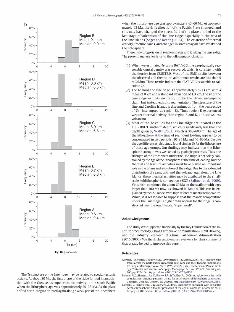
Fig. 10 shows that the Te along the ridge is not changing progressive-ly, but instead exhibits segmentations. The strength of the lithosphereunder region A and E is higher than that of other areas slightly. Mostof the Te estimates in region A and E are 8–12 km, and so these sea-mounts are “flank ridge” features, according to Watts et al. (2006).The continuity of the Line and Caroline Islands is interrupted in regionE. The lithosphere under the Line Islands (regions B and D) is weaker,
−175o −170o −165o −160o −155o−20o
−15o
−10o
−5o
0o
5o
10o
15o
20o
(A)
(B)
(C
(D)
Fig. 9. Minimum RMS misfits between m
and show lower Te of 4–8 km. This means that the Line Islands are an“on ridge” setting. The upper-right corner of Fig. 10 shows the Te ofthe Hawaiian-Emperor chain. As a chain constructed by a “hot spot”,the Te decreases gradually from southeast to northwest, with increasingdistance from the hot spot. This indicates that the Line ridge may havebeen modified by tectonic activities more complicated than those of a“hot spot”.
−150o −145o −140o −135o0.0
1.5
3.0
4.5
6.0
7.5
9.0
10.5
12.0
13.5
15.0mGal/km
)
(E)
easured and theoretical admittances.

70 M. Hu et al. / Tectonophysics 658 (2015) 61–73
Watts et al. (2006) calculated the Te of the lithosphere under morethan 9000 seamounts using the bathymetry predictionmethod and sea-mount database provided by Wessel (2001). In the study area of thispaper, the Te values of approximately 543 seamounts are calculated.Fig. 11(a) shows the results given by Watts et al. (2006). The Te of theLine ridge shows a similar trendwith our results, except for a few valuesgreater than 20 km. Fig. 11(b) shows the differences between our re-sults and those of Watts et al. (2006). Most of the absolute differencesare less than 5 km.
Both theMWAT and the bathymetry predictionmethod have advan-tages and disadvantages when estimating Te. The MWAT takes into ac-count both the near and far zone loads but reduces the resolution. Thebathymetry prediction method can be used easily to calculate Teunder an individual seamount, but it may overestimate Te if adjacentloads are ignored (Kalnins and Watts, 2009), especially for a smoothbasin. Themethod ofWatts et al. (2006) is generally applied to an isolat-ed seamount that has been surveyed by ship soundings, while theMWAT can be used to estimate the Te for nearly the entirety of theseafloor.
4. Discussions and conclusions
The relationship between Te and the age of the lithosphere at thetime of loading is analyzed here. Ages of 21 seamounts were collectedfrom Schlanger et al. (1984) and Davis et al. (2002) (Table 4). There isno clear hot-spot age progression along the ridge. Table 4 also lists the
−175o −170o −165o −160o −155o−20o
−15o
−10o
−5o
0o
5o
10o
15o
20o
(A)
(B)
(C
(D)
a
Fig. 10. Te of the lithosphere under the Line ridge and its adjacent areas (a) and the frequencyshown at the upper-right corner for comparison).
seafloor age at the time of loading and the Te values calculated in thispaper.
The relationship between Te and the age of the seafloor at the timeofloading is shown in Fig. 12.
Both the Te samples of the Line ridge and the Hawaiian-Emperorseamounts are shown in Fig. 12 for comparison. According to Fig. 12,most of the Te along the Hawaiian-Emperor seamounts are located atthe 300–450 °C isotherm depth, while most of the Te along the Lineridge are located at the 150–300 °C isotherm depth. Kalnins and Watts(2009) show that Te of the Cretaceous lithosphere for the northwesternPacific is in the 180 ± 120 °C isotherm depth range, and the results inthis paper agree with this finding. Based on the data along the Lineridge in Table 4, the age of the seafloor at the time of loading can be di-vided into twoparts. Some of the seamounts have ages older than 80Maand formed on 20–35 Ma seafloor, and the other seamounts have agesthat are approximately 70 Ma and developed when the seafloor agewas approximately 40–60 Ma. As shown in Table 4 and Fig. 12, the Teof these seamounts are similar. These results may suggest that the lith-osphere of the Line ridge, as a whole, experienced certain geologic pro-cesses, such as thermal activation, fracture, etc., which weakened itsstrength.
The origin of the Line ridge can be discussed based on Te of the lith-osphere. The Te is the product of a combination of various tectonicforces experienced by the lithosphere. The tectonic origin of the sea-mount chain can be discussed based on Te, seamount ages, bathymetry,and lithology.
−150o −145o −140o −135o0
5
10
15
20
25
30
35
40km
)
(E)
170˚ 180˚ −170˚ −160˚ −150˚
20˚
30˚
40˚
distribution of Te in the five experimental regions. (Te of the Hawaiian-Emperor chain are
0%
20%
40%
60%
80%
Fre
quen
cy
12 16 20
Te (km)
0%
20%
40%
60%
80%
Fre
quen
cy
12 16 20
0%
20%
40%
60%
80%
Fre
quen
cy
12 16 20
0%
20%
40%
60%
80%
Fre
quen
cy
0 4 8
0 4 8
0 4 8
0 4 8 12 16 20
0%
20%
40%
60%
80% b
Fre
quen
cy
0 4 8 12 16 20
Region EMean: 9.1 kmMedian: 9.0 km
Region DMean: 6.6 kmMedian: 6.5 km
Region CMean: 6.9 kmMedian: 6.8 km
Region BMean: 6.7 kmMedian: 6.6 km
Region AMean: 9.6 kmMedian: 9.4 km
Fig. 10 (continued).
71M. Hu et al. / Tectonophysics 658 (2015) 61–73
The Te structure of the Line ridge may be related to special tectonicactivity. At about 80 Ma, the first phase of the ridge formed in associa-tion with the Cretaceous super volcanic activity in the south Pacificwhen the lithosphere age was approximately 20–35 Ma. As the platedrifted north,magma erupted again along aweakpart of the lithosphere
when the lithosphere age was approximately 40–60 Ma. At approxi-mately 43 Ma, the drift direction of the Pacific Plate changed, andthis may have changed the stress field of the plate and led to thelast stage of volcanism of the Line ridge, especially in the area ofthe Line Islands (Sager and Keating, 1984). The existence of thermalactivity, fracture zones, and changes in stress may all have weakenedthe lithosphere.
There is no progression in seamount ages and Te along the Line ridge.The present analysis leads us to the following conclusions:
(1) When we estimated Te using BAT_VGG, the geophysically rea-sonable crustal density was recovered, which is consistent withthe density from CRUST2.0. Most of the RMS misfits betweenthe observed and theoretical admittance results are less than 5mGal/km. These results indicate that BAT_VGG is suitable to cal-culate Te.
(2) The Te along the Line ridge is approximately 5.5–13 km, with amean of 8 km and a standard deviation of 1.3 km. The Te of theLine ridge exhibits no trend, unlike the Hawaiian-Emperorchain, but instead exhibits segmentation. The structure of theLine and Caroline Islands is discontinuous from the perspectiveof Te (interrupted at region E). Thus, region E experiencedweaker thermal activity than region B and D, and shows lessvolcanism.
(3) Most of the Te values for the Line ridge are located at the150–300 °C isotherm depth, which is significantly less than thedepth given by Watts (2001), which is 300–600 °C. The age ofthe lithosphere at the time of seamount loading appears to beconcentrated in two periods: 20–35 Ma and 40–60 Ma. Despitethe age differences, this study found similar Te for the lithosphereof these age groups. Our findings may indicate that the litho-spheric strength was weakened by geologic processes. Thus, thestrength of the lithosphere under the Line ridge is not solely con-trolled by the age of the lithosphere at the timeof loading, but thethermal and fracture activities must have played an importantrole in the origin and evolution of the ridge. Due to the extendeddistribution of seamounts and the volcano ages along the LineIslands, these thermal activities may be attributed to the small-scale sublithospheric convection (SSC) (Ballmer et al., 2009).Volcanism continued for about 60 Ma on the seafloor with ageslarger than 100 Ma now, as showed in Table 4. This can be ex-plained by the SSCmodelwithhigh referencemantle temperature.While, it is reasonable to suppose that the mantle temperatureunder the Line ridge is higher than normal for the ridge is con-structed near the south Pacific “super swell”.
Acknowledgments
The studywas supported financially by theKey Foundation of the In-stitute of Seismology, China Earthquake Administration (IS201506205),and the Industry Research of China Earthquake Administration(201508006). We thank the anonymous reviewers for their commentsthat greatly helped to improve this paper.
References
Atwater, T., Schlater, J., Sandwell, D., Severinghaus, J., & Marlow, M.S., 1993. Fracture zonetraces across the north Pacific cretaceous quiet zone and their tectonic implications.In: Pringle, M.S., Sager, W.W., Sliter, W.V., Stein, S. (Eds.), The Mesozoic Pacific: Geol-ogy, Tectonics and VolcanismGeophys. Monograph Ser. vol. 77. AGU, Washington,D.C., pp. 137–154. http://dx.doi.org/10.1029/GM077p0137.
Ballmer, M.D., Hunen, J., Ito, G., Bianco, T.A., & Tackley, P.J., 2009. Intraplate volcanismwithcomplex age–distance patterns: a case for small-scale sublithospheric convection.Geochem. Geophys. Geosyst. 10, Q06015. http://dx.doi.org/10.1029/2009GC002386.
Calmant, S., Francheteau, J., & Cazenave, A., 1990. Elastic layer thickening with age of theoceanic lithosphere: a tool for prediction of the age of volcanoes or oceanic crust.Geophys. J. 100, 59–67. http://dx.doi.org/10.1111/j.1365-246X.1990.tb04567.x.

−500
0
−500
0
−5000−5000
−5000
−500
0
−5000
−5000−5000
−5000
−5000
−5000
−5000
−5000
−4000
−4000
−4000−4000
−4000
−40
00
−4000
−4000−3000
−3000
−3000
−3000−3000
−200
0−175o −170o −165o −160o −155o −150o −145o −140o −135o
−20o
−15o
−10o
−5o
0o
5o
10o
15o
20o
0
5
10
15
20
25
30km
(A)
(B)
(C)
(D)
(E)
a
−500
0
−500
0
−5000−5000
−5000
−500
0
−5000
−5000−5000
−5000
−5000
−5000
−5000
−5000
−4000
−4000
−4000−4000
−4000
−40
00
−4000
−4000−3000
−3000
−3000
−3000−3000
−200
0
−175o −170o −165o −160o −155o −150o −145o −140o −135o
−20o
−15o
−10o
−5o
0o
5o
10o
15o
20o
−15
−12
−9
−6
−3
0
3
6
9
12
15km
(A)
(B)
(C)
(D)
(E)
b
Fig. 11. Lithospheric effective elastic thickness under certain seamounts of the Line ridge given byWatts et al. (2006)(a); and differences between results calculated in this study and that ofWatts et al. (2006) (b); (Background contours are based on bathymetry model BAT_VGG).
72 M. Hu et al. / Tectonophysics 658 (2015) 61–73

300
600
900
−80
−70
−60
−50
−40
−30
−20
−10
0
Dep
th/E
last
ic T
hick
ness
(km
)
0 20 40 60 80 100 120 140 160 180
Age of Oceanic Lithosphere at Time of Loading (Ma)
Unit: oCP&SGDH1
Hawaii_EmperorLine Seamounts (this paper)Line Seamounts (Watts et al., 2006)
Fig. 12. Relationship between the effective elastic thickness and the age of the oceanic lith-osphere at the time of loading. (P&S: model given by Parsons and Sclater (1977); GDH1:model given by Stein and Stein (1992). Purple squares represent the results from thispaper, red circles represent results from Watts et al. (2006), and blue triangles representthe results for the Hawaiian-Emperor seamounts).
Table 4Seamount ages and Te of the Line ridge.
Samples'name
Location Age ofseafloor(Ma)
Age ofseamount(Ma)
Age of seafloorat time ofloading (Ma)
Te(km)
143D_102 169°03′W,19°30′N 110.8 88.1 22.7 13.2142D_11 169°05′W,18°00′N 114.2 93.4 20.8 10.8RD63_7 168°13′W,16°27′N 115.3 86.0 29.3 8.2RD59_12 167°03′W,12°31′N 120.6 85.0 35.6 8.7RD61_1(5) 166°27′W,14°59′N 113.8 82.0 31.8 8.9128D_11 160°45′W,09°15′N 112.8 78.7 34.1 7.3RD33_1 161°55′W,08°11′N 118.6 39.3 79.3 7.2123D_15 160°45′W,05°50′N 122.4 76.4 46.0 6.5PCOD_6_2 158°30′W,02°35′N 119.5 69.8 49.7 6.0RD41_1 157°21′W,02°06′N 115.1 35.5 79.6 5.6RD43_1 155°17′W,00°42′S 108.0 59.0 49.0 6.9RD44_3 151°33′W,07°35′S 93.7 71.9 21.8 8.7RD45_26D 150°42′W,09°04′S 90.7 70.5 20.2 7.4RD52_1(2) 149°02′W,15°01′S 66.9 44.6 22.3 8.2Johnston Atoll 169°17′W,16°44′N 118.9 71.2 47.7 7.7Keli RidgeWest 170°24′W,15°42′N 121.5 70.8 50.7 8.6Keli Ridge East 169°12′W,15°36′N 119.3 67.6 51.7 7.7Smt.14N170W 170°00′W,14°00′N 125.6 68.1 57.5 8.1Smt.10N162W 162°00′W,10°00′N 114.7 83.6 31.1 7.7Smt.9N165W 165°00′W,09°00′N 125.6 69.3 56.3 8.5Kingman Reef 162°54′W,06°18′N 125.3 70.0 55.3 7.2
Annotations: The sample names, locations, and ages are from Schlanger et al. (1984) andDavis et al. (2002). The age of the seafloor is interpolated fromMüller et al. (2008). The ageof the seafloor at the time of loading is defined as the age difference between the seafloorand the seamounts. Te is calculated by MWAT using the bathymetry model BAT_VGG andaltimetric gravity anomalies SIO V20.1.
73M. Hu et al. / Tectonophysics 658 (2015) 61–73
Conrad, C.P., Bianco, T.A., Smith, E.I., & Wessel, P., 2011. Patterns of intraplate volcanismcontrolled by asthenospheric shear. Nat. Geosci. 4, 317–321. http://dx.doi.org/10.1038/NGEO1111.
Davis, A.S., Gray, L.B., Clague, D.A., & Hein, J.R., 2002. The Line Islands revisited: New40Ar/39Ar geochronologic evidence for episodes of volcanism due to lithospheric ex-tension. Geochem. Geophys. Geosyst. 3. http://dx.doi.org/10.1029/2001GC000190.
Hu, M., Li, J., Li, H., Shen, C., Jin, T., & Xing, L., 2014. Predicting global seafloor topographyusing multi-source data. Mar. Geod. http://dx.doi.org/10.1080/01490419.2014.934415.
Kalnins, L.M., & Watts, A.B., 2009. Spatial variations in effective elastic thickness in thewestern Pacific ocean and their implications for Mesozoic volcanism. Earth Planet.Sci. Lett. 286, 89–100. http://dx.doi.org/10.1016/j.epsl.2009.06.018.
Lynch, M.A., 1999. Linear ridge groups: evidence for tensional cracking in the Pacific plate.J. Geophys. Res. 104 (B12), 29321–29333. http://dx.doi.org/10.1029/1999JB900241.
McNutt, M.K., & Judge, A.V., 1990. The superswell and mantle dynamics beneath the southPacific. Science 248 (4958), 969–975. http://dx.doi.org/10.1126/science.248.4958.969.
Morgan, W.J., 1972. Deep mantle convection plumes and plate motions. Am. Assoc. Pet.Geol. Bull. 56 (2), 203–213.
Müller, R.D., Sdrolias, M., Gaina, C., & Roest, W.R., 2008. Age, spreading rates, and spread-ing asymmetry of the World's ocean crust. Geochem. Geophys. Geosyst 9 (4), 1–19.http://dx.doi.org/10.1029/2007GC001743.
Nakanishi, M., 1993. Topographic expression of five fracture zones in the northwesternPacific ocean. In: Pringle, M.S., Sager, W.W., Sliter, W.V., Stein, S. (Eds.), The MesozoicPacific: Geology, Tectonics and VolcanismGeophys. Monograph Ser. vol. 77. AGU,Washington, D.C., pp. 121–136. http://dx.doi.org/10.1029/GM077p0121.
Natland, J.H., 1976. Petrology of volcanic rocks dredged from seamounts in the LineIslands. Initial Rep. Deep Sea Drill. Proj. 33 (26), 749–777.
Parsons, B., & Sclater, J.G., 1977. An analysis of the variation of ocean floor bathymetry andheat flow with age. J. Geophys. Res. 82 (5), 803–827. http://dx.doi.org/10.1029/JB082i005p00803.
Sager, W.W., & Keating, B.H., 1984. Paleomagnetism of Line Islands seamounts: evidencefor late Cretaceous and early Tertiary volcanism. J. Geophys. Res. 89 (B13),11135–11151. http://dx.doi.org/10.1029/JB089iB13p11135.
Sandwell, D.T., & Smith, W.H.F., 2009. Global marine gravity from retracked Geosat andERS-1 altimetry: ridge segmentation versus spreading rate. J. Geophys. Res. 114(B01411). http://dx.doi.org/10.1029/2008JB006008.
Schlanger, S.O., Garcia, M.O., Keating, B.H., Naughton, J.J., Sager, W.W., Haggerty, J.A.,Philpotts, J.A., & Duncan, R.A., 1984. Geology and geochronology of the Line Islands.J. Geophys. Res. 89 (B13), 11261–11272. http://dx.doi.org/10.1029/JB089iB13p11261.
Smith, W.H.F., 1993. On the accuracy of digital bathymetric data. J. Geophys. Res. 98 (86),9591–9603.
Smith, W.H.F., & Sandwell, D.T., 1994. Bathymetry prediction from dense satellite altime-try and sparse shipboard bathymetry. J. Geophys. Res. 99, 21803–21824.
Smith, W.H.F., & Sandwell, D.T., 1997. Global seafloor topography from satellite altimetryand ship depth soundings. Science 277 (5334), 1956–1962. http://dx.doi.org/10.1126/science.277.5334.1956.
Stein, C.A., & Stein, S., 1992. A model for the global variation in oceanic depth and heat flowwith lithospheric age. Nature 359, 123–129. http://dx.doi.org/10.1038/359123a0.
Walcott, R.I., 1970. Flexural rigidity, thickness, and viscosity of the lithosphere. J. Geophys.Res. 75 (20), 3941–3953. http://dx.doi.org/10.1029/JB075i020p03941.
Watts, A.B., 1978. An analysis of isostasy in theWorld's oceans: 1 Hawaiian-Emperor sea-mount chain. J. Geophys. Res. 83 (B12), 5989–6004. http://dx.doi.org/10.1029/JB083iB12p05989.
Watts, A.B., 2001. Isostasy and Flexure of the Lithosphere. CambridgeUniversity Press, London.Watts, A.B., Sandwell, D.T., Smith, W.H.F., & Wessel, P., 2006. Global gravity, bathymetry,
and the distribution of submarine volcanism through space and time. J. Geophys. Res.111 (B08408). http://dx.doi.org/10.1029/2005JB004083.
Wessel, P., 2001. Global distribution of seamounts inferred from griddedGeosat/ERS-1 altim-etry. J. Geophys. Res. 106 (B9), 19431–19441. http://dx.doi.org/10.1029/2000JB000083.
Wilson, J.T., 1963. Evidence from islands on the spreading of ocean floors. Nature 197,536–538. http://dx.doi.org/10.1038/197536a0.
Winterer, E.L., 1976. Bathymetry and regional tectonic settings of the Line Islands chain.Initial Rep. Deep Sea Drill. Proj. 33 (25), 731–748.
Zhang, J., Jin, X., Gao, J., & Zhao, L., 2006. Influence on the seamounts' formation in MPMand WPSP from fractures and cretaceous magma's activities. Mar. Geol. Quat. Geol.26 (1), 67–74 (in Chinese with English abstract).