" fleD /2O2.'o2-6l

¢0

I'

THLENVEJST FMISSIP"r •r

DEr"'.PARM; O H ST N

79 08 2 8' O0

•'• ..... L.

.... ... ..- .: . '

S~Propagation of Sound Through the Atmosphere:

g•.. Effects oi Ground Cover II

i ~It. E. Bass and L. N. Bol~en

[[-[ Technical Report

~~ ,tily 1979

k ~U. S. Army Research Office

r

,. 4Phyfical Acoustics Research Group Cv 4

The Unive.sity oa MLssisslppi

University, MS p8677

Approved for public release; Go

distribution unlimited.

.... , 4 . . . , . : : . .~ . . q ~ ~i ~ , cza s -.

rifI¶ ~ A%*qIrIrATInN OF THI% "Arir (Whm'flol #I'.Inlsnrd)

REPORT DOCUMENTATION PAGE :APJI";

4 IT F(ad 0,11e)S. TyPF OF REPORT & PEPt'jr~ ,~ .

Propagation ofapund Through theAtmosphere: Final June 1976-19719E ecs f rond Cover II

AU TORa)ff -. _:OTRAQ-T NGAfNUek'.

*H. E.1 as )d L. N. ole., DAAQ- ~9-7-G- 7258

1PERFORMING ORGANIZATION MAMIE AND ADDRESS 0.PGAMELEMENT. PRriJJCT, T A,'V

It. CONTROLLING OFFICE NAME AND ADDRIESS

Research Triangle Park, NC 2770914~+OEI,~jft. fromv Cmntroflgnd Office) 1S, SECURITY CLASS. (of Uthi roporf)

rinal rapt, 1976-19790 Unclassified15s. DECLASSIFICATION/OOWNGRAOING

SCNEDULE N/A

IS ~ ~ ~ ~ " WeT~UT OWNW i.. ..

Approved for public release; distribution unlimited.

'7. DISTRIBUTION STATEMENT (of Cho abstract aitered in Block 20. It different frmi Report)

N/A 4L 6o,~-FLV,-I

16. SUPPLEMENTARY NOTES-

The findings in this report are riot to be construed as an official Depart-mient of the Avmy~ position, unless so designated by other authorized documents.

19. K EY WORDS (Confinu* an reersre @146 It necoeeiwy mid Identify by block niwipbor)

Sound Propagation; Atmospheric Acoustics; Ground Impedance

'20. A 1rA ACT (Cm@h~ is reverse otEo N neusoinp am, Identif bV block inmber)

Measurements of sound amplitude in the vicinity of a ground plane havebeen made as a function of frequency of the sound source (50 Hz -2000 Hz),distance of propagation (Sm - 300m), and surface conditions. By treating theimpedance as an adjustable parameter, the surface impedance as a function offrequency was determined from the measured amplitudes using a theoreticaltreatment of a spherical wave in the vicinity of a locally reacting surface. ~

DD ~¶ 3473 EDITONOF9OVSSS@SSO.ETEUnclassified /.6 jSECUWITY CLASSIFICATION OF THIS PAGE (WhenPmiota Entered)

~~ ~ ~ ~ ~ Lc r~i.L h j ~

It .I"IeI (LA•A% F IC AIION Of THIS PAOCtIf 00a Ite re.E

T1he impedance measurements covered the frequency range 5o Ii,- to 1o00( lz.In this frequency range, the results for three distinctly different surfacessuggest that the impedance can be computed from the specific flow resistanceand that grass has little effect on the surface impedance except for decreasingthe flow resistance due to the root structure, Experimental studies of surfaceimpedance should include measurements of soil parameters such as density,specific flow resistance, and moisture content so that compa-isons can be 1w-debetween the results from different laboratories and so that a data base foradditional theoretical development can be extablished.

o nffi

la•'t l£tcTV CLSIICTO on THIS PAF*%-DteFvee

i -

UnclassifiedaucumInIT Ci-ASSIPIlCATION OP THIS PAOF(It7en bate Frite~.).i 1-

';/

TABLE OF CONTENTS

Page til1. Introduction 1

2. Experimental Technique 3 i2.1 Sound Sources 42.2 Amplitude Measurements 5

2.3 Measurement of lEnvironmental and Soil Conditions 6

3. Experimental Results 93.1 Comparison reasurements 93.2 Determination of Acoustic Impedance 18

4. Interpretation of Results 22

5. Application of Results 42

6. Summary and Conclusions 46

7. Bibliography 49

•4

.L0 INTRODUCTION

rzopaga tion of sound outtdoors Is inf luenced by a variety of mechanismsA

which change the ampl ituie •tind phase ot the wave. These include:

o Atmospheric Aborpti.)fl

$to'ititirv LI lect stI

o Turbulence

o RetF raict ionl.

In previous studies, atmospheric absorption was considered in terms of

microscopic processes and a technique was developed which allows one to

pr'edict ktmosphoric absorptioon using simple expressions which are based on

the rigorous microscopic treatment (Ret. 1-5). At low frequencies (-I kllz),

for most conditions, the presence of a boundary will effect the sound amplitude

more than atmospheric absorption (Ref. 6). An earlier report (Ref. 7) Jconsidered this mechanism for frvlUcuc es bCtween 100 ltz and I kHz for a

field of institutiotnal grass and a field of Sorghum Sudaln grass. This re-

p .rt will expand the Low frequency range and soil types discussed in the earlier

report. rurbulence can also effect the sound field by destroying coherence

and thefreby CeduCIlCng interference which would otherwise occur in the presence

ot a boundary (Ref. 8). Refraction due to a thermal or velocity gradients

also influences the received sound. The measurements reported here were

taken under conditions which minimized the effects of turbulence and refraction.

This study of the effect of the ground on outdoor propagation of sound

through the, atmosphere Is the second step in a long range effort to develop

procedures to reli[ably predict sotnd amplitudes a significant distance from

the source and correct measured spectra to free field conditions.

I.5

tf..'

This report deals primarily with experimental measurem,fnts of sound

ampi itude in the vicinity of 4 ground surlace at ranges out t- 300 m at

frequenicies between W0 IIz and )00 Itz. These measurements serve primarilyIt extend the data base for surtace Impedances. This report includes the

findings in Rtference I related to surtace impedances but omits the acoustic

to seismic mesurements and computer programs included in that earlier report.

The experimental and theoretical work on the problem of outdoor sound

propagat ion undertaken by this laboratory is meant to complement similar

efforts being made by other laboratories most notably the acoustics group

at the Nar:ional Research Council of Canada (Ref. 4-1l), and Wyle Laboratories

(Ref. 8).

The experimental techniques employed to generate the sound field and

measure sound amplitude are described in Section 2. in Section 3, the ex-

perimental results are presented. Due to the large number of measurements

made, tile results are most often reported in terms of acoustic impedance

values deduced from a model of the ground surface. Should this model, at

some later date, be shown to be inadequate, the raw experimental data can

be reconstructed by using the deduced impedance values to calculate the

measured sound amplitude. Section 4 provides a tentative interpretation

of the experimental results. Section demonstrates how these results can be

used in a practical application and Section b summatizes the results of

this study.

2 I

2.0 EXPERIMEMTAL TECHNIQUE

The measurements were made by broadcasting bands of sound over prepared

fields from 300 to 1000 feet in length. Microphones were placed at intervals

down the range at two heights, and recordings were made of the SPL of each

microphone. These recordings were then analyzed to determine the surface im-

pedance values of the grounds. Four fields were used for these measurements.

I) Band Field and Softball Field at the University of Mississippi. The

band field represenced a typical institutional grass field with a hard

non-porous clay soil and low moisture content (density 1300 kg/m3 dry).

This field has been undisturbed for at least 15 years. The softball

field also consisted of a grass covered clay soil (density 1450

kg/in3 dry). It, however, was prepared with dirt fill two years ago, Iand the grass cover is not as complete as at the band fleld.

2) Experimental Range at the Waterways Experiment Station in Vicksburg, Ms.

This field consisted of a brown to dark brown heavy silt !cam with

subsoil ranging from heavy loam to silty clay loam. Measurements

were made with two different noisture contents.

j) Farm near Oxford, MS., The soLl and vegetation on this farm was prepared

for these measurements, and soil classific&cion was made by the USDA

Sedimentation Laboratory in Oxford. The site was located in a valley

bottom covered with recent alluvium deposited over Kosciusko aad

Tallahatta foundations The soils are palevdalts and are predominantly

a silt loam with greater than 50 percent silt and 7 percent clays (1470

3kg/mr dry). The region between 200 and 350 feet on the test range contains

I-

[•' i '3

[,• 'i

I.

more IOamv sand. M,,asurementts were made bet ore the field was plowed,

on a bare plowed lIeld, on t hi tI eld with va rious I ieigh ts of Sorghum

21

•o ~~~Sudan grass, and t,n .i ha~re f ield af ter harvest. III vach caste mePasur-ll lt-

S~Mellt.,- Were Made• Witth VariotS nMOiStttrV Conttntli. -A

4) Sandy Farm near England Air Force Base, Florida. This field was A

bare ot vejý%tattion and measuremewt s were made with varioues moisttu ro

coentt. ts l't, s.i,, was utniform to a depth of six feet over tihe 1000

I oot tange.

: ) Sardis Reservoir Beach. This areit was hare of veget at ion with six

itiches to a toot ot loose sand overlying a ,I'av base.

_. 1 Several speaker systems were constructed for this project. Au

Alttc '- S1B IS inch diameter bass driver itn a ducted port enclosure was used

for the data taken at tht" Waterways Experiment Stat ion. A combination of 4

ot these speakers in all l ect rovoice TI. 60tQ enclosure was used for mid-low

frequency measurements (100-200l Hz). The extreme low frequency data (40-100 liz)

were taken using a EVI8B speaker in a modif ied Electrovoice Mb 5,05 ec closutro.

IHI igh frequency data (200-2000 l1z) were taken with a horn system composed of ,

"Unnivorsitv ID-W compression drivers loaded by an inverted cone truncated with "

a 4 inch diameter opening.

the data analysis program assumes a spherically diverging wave froent.

Although a theoretical treatment for a non-spherical wave is possible, tile

spherical geometry eases physical interpretation ot the results. The require-

mernt for a spherical wave front dictates that the source of sound be approxi-

mated as a point source. At frequencies below 100 Hz, this represents no

problem; the speakers used can be considered a source of spherical waves. Each

speaker system utilized was tested Lo determine its directivity pattern as a

4

I1

funct ion of frequency. An increased directionality at higher frequencies is

characteristic of radiating circular pistons. As a result of these measure-

ments, data Above 200 Hai were not taken using the large. low frequency driver

systems. The high frequency system was capable of producing a uniform dis-

tribution of sound with a deviation from sphericity of t2dB to a frequency of

2000 117..

2.2 Measurements were made of the amplitude of the sound by microphones

placed I and 2 meters above the surface of the ground at 100 foot intervals

from 50 to 1000 feet from the speaker. A single stationary reference micro-

phone was placed at ground level 50 feet from the speaker to measure any vari-

ations in sound intensity from the speaker system during the course of the

experiments.

Two types of signals were broadcast over the range. Octave bands of

pink noise of one minute duration were used in the original experiment at WES.

Later data taken at the fields in Oxford and Florida used bands of pink noise

1/2 octave in width centered about each 1/3 octave center frequency from 40

to 2000 Hz. Data were also taken in Oxford using sweep test tones from 80-

200 Hz and 180-2000 Hz. In each case the appropriate speaker system was used

to assure the sphericity of the transmitted wave.

The speaker system was suispended on a large crane at WES and speaker

heights varied from 1 to 10 meters above the ground. In Oxford, the speaker

system was suspended from a cross member on a telephone pole placed in the

field, and most of the data were taken with a speaker height of 10 feet. A

portable A-frame stand was constructed for use on the bar,0 field, at Sardis

Reservoir, and in Florida. This permitted speakers to be suspended at heights

up to 10 feet above the ground.

5

Ski

The mi,:rophones used for the amplitude measurements were B&K 4125 1/2"

Condenser Microphones with B&K 26.2 preamplifiers and B4K 3810 power supplies.

A GR 1962-9602 Electret microphone was used to monitor the speaker level. The ,i

signals from the microphones were recorded at various times on a pair oi Uher

4200 2 track tape recorders, a Tandberg 4 track FM recorder, and an EMI 8

track FM recorder in special environmental packages. These data were then

played back originally into a GR 1554-A 1/3 octave band analyzer for the anal-

ysis of pink noise or into a HP 3480A analyzer synchronized for use as a

tracking filter for the sweep test tones. The later data were analyzed using

a computer based GenRad System 1923.

The system was calibrated by recording the output from a GR 1562 sound

level calibrator on each microphone-recorder channel at the beginning and end Nof each run. No measureable gain shift was observed during the course of any

run.

2.3 Differences in air temperature with height above the earth may have

a strong effect on the propagation of acouatic waves due to refractive effects.

Measurements of air temperature versus height were made at each site during

the course of each test period. The temperature and wind velocity was moni-

tored using a Wallac GGA23S Thermo-Anemometer with a NiI25ANE probe. A log

was kept of these variables during each testing period. Temperature gradients

of less than 3*F for a 10 meter height increase were always required for data

acquisition and in general the gradients were less than 20F for 10 meters.

Data was not collected when the wind speed exceeded 3m/sec.

An estimate of the effect of air turbulance on the acoustic signal was

obtained by measuring the coherence length of the propagating sound waves.

6

Sinke it single source was producing the direct and reflected wave, Interfer-

tence eflects from phast, cancellation could be observed only If tihe waves were

k'(herent over the path length involved. White noise and bands of pink noise

were broadcast over the range. The acoustic signals received by microphones

30 meters apart were analyzed on a Honeywell SAI43A Correlation Analyzer. U

'rlie coherence length medsured in these experiments was greater than 30 meters

for the noise. The coherence length is frequency dependent and it will be Anoted in the results that above 1 kHz, turbulence led to a loss of coherence Iat the greater propagatian distances.

Moisture content of tile soil can greatly affect its flow resistance

and acoustic properties. The soil was sampled at the time of each measure-

ment and the flow resistance and water content was measured and included

as a parameter in each of the measurements reported. The specific flow

resistance of each soil sample was measured using an instrument constructed

using a design of Leonard'2 A cylindrical sample of earth was taken

from the field and the rate of air flow through the soil sample was

measured as a function of differential pressure across the sample. Measure-

rments of flow resistance were made of each soil sample using at least threeA

differential pressures across the sample. Consistency of these results were

alway, within 5%. However, it was found that there were inconsistencies in

the measured flow resistances from multiple samples removed from thesame fields. Values )f flow resistance which varied by as much as a

tactor of 2 were observed in some fields, although measurements of the flow

resistance of sand were consistent to within l0%. It was assumed that these

discrepancies occured because of variations in soil structure in the 10 cm

diameter plugs extracted for measurement and the effects of disturbing the soil.

Root structures, fissures and inhomogenities in the loosely packed soil at the

7

-- ~ ~-42 -A

I arm res, it ed I u Lh 'lit I argust v, la t h t ons. 4till, Ian Io 1-1' m• ist .q•sld in FIlor Id:a

pv rm, It L vd mtrio ' IV arol• O. U ti- s oil . S14l0 1M1 I bV I) .S' 1t .S •4, a•1d r •, l-ti I ed In I( ho

1llos E.S 1 00 it ' tlS I Lull t. restil I1t. . 'Thu va I tat's f f I 1ow rs Is, . t. c'v reported iJ re' ti t,

aivsrrage va lues of t lit samp Ie ts Lken at each I Ifvl d dur lIg t htc dav of t le

acoust ic; I inleasureMValnLS. '

The wet and dry weight of a layer soil sample was re.orded to dltermine,

mr()i.sture content. A plug of topi soil of cylindricoal cross se'tlIon 30 Vlm Ill

di hi~eter was removed from the f 'eld. encased in a ptilast Ic •ag and weighed.

The .SoIl was then dried in an a i r condi i toned env i r(,melnt nti II weight va r 1it i(ills

(,eased, and tile percteuL moisture content of the sample was recorded.

4I,

'4;2

[H

D EXPERIMENTAL RESULTS

H i ý Weroco Iot t d 11 1v Ig vus 1 r t Isinops is kii t hit- varloous aa

licgolin

s I i iv o lon Ie glt s, ndt pI a I\1V)d fefvrenit f ro (I en I ts . Al I data welre

I'IirvI,-i it) noW.V to put-sonit at I Ithis dat a In a report tit accelitable IlengthI.

lutcdont y thAt dilt. nleeded to illuistrAte specifi c bits, wil I Iti presentvtd.

Ftilithtcr, thil- dat a will be discussed i n t he order appropr iatv t o a I og ical

devel opieivia kit thlit toplicv, not in theil order in whiichi t liywere col I ect ed.

1.1 I (lit .-i r I son-i Nea s tii ren t, ~. nts

T'he ground cover most. thoroughll st udied lin terms tit a boundlarv to acotiqt ic

p rop.ugt Iokil is inst i t niL tonal grass"' hI'Is th ltype~t cover usim I Ix ynonvom oreil

on i'I I CgV C.ra1Mp S I lwuiS , .1 tu'iid goVe milieu 01t 11111 (1I i ng)S , et k,. AlIt hotigh t lit, ac t tia

gast vlj Varies, iL Is- almost always wellI t r immed , uniform. and re) at i vi v

dent-e. The earth, 1 unider t lie, grass has tistia I I v gone manyv grow ini sea.SOnIS W it It-k

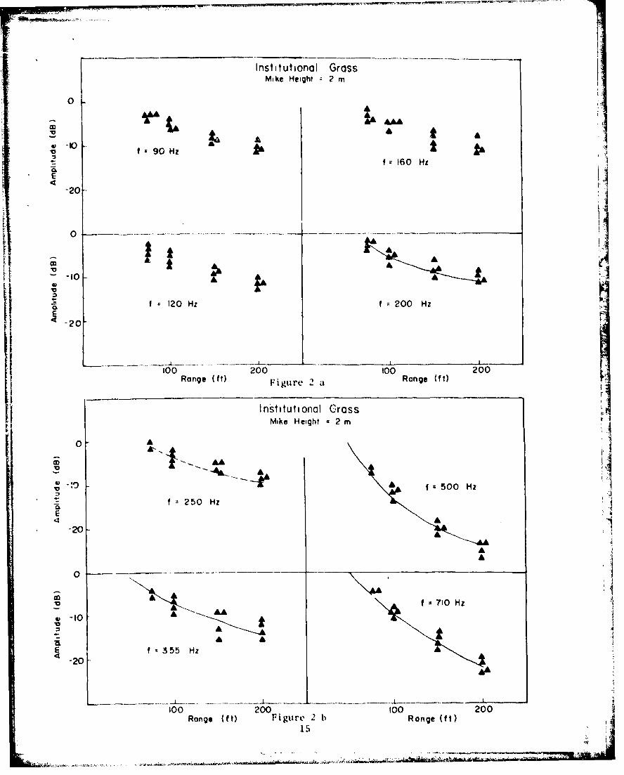
Mesueon t o sound amlp I I t tidle over Inlst It tit IonalI grass on t he till I veus I t v

o I M Is I 8 I pp I (UNM) c~amlptu ax presu)'ulint ld I it Figutrels 1 - 2. AllI lvelIs are ie il rencevil

to t he ')0 ft . posit [til. Thoese data (Runs I I and I2) Were -OIl Ivctl'( with Ow.li spea~ker

sv t em .I t f rom t he grouind pl ant' and two iii it, roplliones (one inet er and two muet irs

ablovk Llit,' ground) wil livIt weti' moved bet weeui dal a col e I Ivition liucat Ions Wi I t

7 t I . I 100 I t. 1 '1 1 t I. ,and 200 ftL. f riulu t lie, speako'i 'llue source was dIrkIven

I lo

-Jr- -- r r, rl r

'V * F ~ 4 .4". 41

C) U 0 90 0.,4 C) -42~~.1 cu) 0

0V V) U) l

4-H 0 0a 06M a w

0 N Nu N'

0 4144. 00

4-4 rV) CD 0

C1 '4 00 4 -,

1-4 CD c'V C

0

00 't) 0 x0 .

0-4-

tn 00 WO~ I~

".4 1-ao -("

(N -I C '~CN C-4 (- 4~'4.

IV rCA, N~. C), o- O '

04. j aj N (I r 'mw>0 00Hu ~ 71 11 0 W' > 0,'1) () 4) i I0&C. O N (r) -( U ) C).7uLAa w oIN

C 'c

C) C .- j C1- C ) '

X-4 4W 4

t44 1-4

II

0~,

ý"44

-4 -4

IV -4'H) r,.. 4,1

C; 0 U a 0

117 (v m LP-4 E -'4 ý'O 4bO '-3"u4 '-4 1-. I- A

Cl C),

-~ *00 0 ' .44-1,4 _a ui U ) 144 44 ()

'-4 *HýD . -4 -4 -4 a 14-is

00 0 0 v

00 -4 0 04

U)~~a 1f4)U)r

t-4 J-4

LIZ

00~ clc

', -r -4-

___ __ ___ __ ___ __ ___ ___0tM46J

0 0 .0

to o 0N NN

4~ -4 W . ~ *-

0t rd V 0'-4 :3u

4a

'Aj Q)

ILI

0

-4 U UlOci v

Cdq

'-44

_•~ ~ ~ ~ ~~~~~ ~~~~~ ..• . .• •r• .. . •.. • •-;••..: . • • • • • .•• : .; .. . . ... ,•:,;; • . . . . • . . . .; :•

Institutional GrassMike Height = I m

0

rA A f:6A1L

t f =90 Hz f 160 Hz

..kF

< -20

0

At I

-A A'AA

A

Sf 120 Hz f : 200 Hz

100 200Range (ft) Figure 1 a Range (ft)

Institutional GrassMike Height I m

0

"0- A H500H zAA

-- 10

AA Af 250 Hz A

E

--20

A

0-

Alo- fa 710 Hz

f 355 Hz A A ~'A

< -20-

_ _ _ _ _ __,.AI

100 200 100 200Range (ft) Figure 1 b Range (ft)

13

------------------------------- ~- --- Ai--

Institutional GrossMike Height I m A

AAA LA

0f 1000 Hz

AL1jI0 f 2000 Hz A

S A4

"0 A

AA

vAA

.10

f :1400 Hz A

"= -20 A

100 200 100 200Range (ft) Range (ft)

Figure 1 c

14:It1

-. -,. . __I• , • a •t.. . . ... ..... ..- ,. - .. .. . ....... . - . .. . . . ....... K• • t . . .J"• 4"1• "

Institutional GrassMike Height 2 m

0

A

AA

f 910 Hzf 160 Hi4

E-4V

"-20

0 -- A -I- .A

A

-10 ALIA

f 120 Hz f 200 Hz

-20,

100 200 100 200Range (ft) Figure 2 a Ran ge (ft

- In'stitutional GrassIMike Height 2 m

0A

f 50H HzI: 2 AA55H Hz

Er

ýAAA

0

A 4

.~I0A AA

A A

E f 355 H-20-

100 200 100 200Range (ft0 Figure 2 b Range (ft)

-=-1

Institutional GrassA Mike Height 2 m

f -2 kHz

.10 f10 ~

a £z

"-20LA IA

-20-

Range (ft) Range (ft)

16

~~~~~~~~f 140 Hz ••t•""",,: `:••'' "=

o' a1 pi' Itcc i' id d o swvip t ok t,' x t IInd i ng t rom i 201) lz t o 2 kII., Run II) ,i-i k '

I1.' to ._00it) (Run 12). I

!-V R terriing t.o F igut'i es 1-'2, t canl he -cell kthat hi, ,l:lt t Iw ,- ,c i iow I

.t't' e' 1 c i1 • to w , th ill ,lbout 2 dli., l'h'l i N. va r i , io ki ll pc roba " I v b.

St at irut td to' vriat ionls ill 'ýpakvr output, ilo ist, Mnd inst ahi lit i s ini t. I3

rcordking sv,stenti. A va -'it at oi 0 dt B was ant Ic 1 a t d t,-ix is 'onsitdvrvti

"acceptallb '. At tthe Iatrgetr tange ilt, tfluct I i at iols exceed t d T, Th i s i :

Sresuilt ot decreased ignatl to noisi rat't bt' hut stincc this type of scatte r should

be random. by tak ing I our points, tlie t utt SFI. should be de, ermined ± 1 dB.

As t lit I requctitv intitreases, so does Ltitw Itctter in dat a. At 500 HIz this

Situat ionl is worst The f i rst tnt er"•ernctte iinitnim occurs near 500 11 !' At

Lilt, int t'terrence mniltinilum, tilt, acous, t ic signal decreases by as much -is 10 dB

therebyv decreasing thi S/N vratik hcv a I ikc amomnt. Al so, qtince intteorference,

rolo.s Oi cohenut'elv between the diret't and refletcted waves. when tht, 'et flet ioa

covitic i ct is high (as it was tor t he tfield uosed) a small I as-s of cohlerencev

duc t o I t rans tent tu'rbi It wi IlI great IV .0 te,-t the ieIeorded M'I. This 'omibilna-

t ioni ol fact'.rs reacht's a max imllum eat" thit, I t'at i nterterence iniilmum in Wmost

a l 1 cases. Since tlie t, vI I, t 01 tkIrI I ecllnkv and n oikis is to iI,'kclaae t lit SPI.,

the low.,st valut of 8S;L. should bc t.iki ais the correct value unless it is much

dilterent from tOw Ken'rltI tr'ld e ,t til, dataa. In 1r,,'1t icek , tilt lowest vAiuOes

Were Weigl tea by a t a.'tol Of two t'ta. ive to inttrmediate valutes (wight ing of

I) whenll conparilng LO tbeatt i,'a 'res.

Referring again to Figure., I and 2, the solid lines wtere computed from

t'.ie theory of )lon 1 using the impedance as an adjustiable parameter to

act' ieeve tIlk best fit bht wein L he0 cv and expe, rimen1t. It t' be senll t ht tIlk'

the'orv is in excel lent agreement with measurvtemnt . As wil.1 be di scusused Iatttur.

17

theste tturei are re Iat ive y v iti nepllndent of va I ues chosen for t he I|mpedanct. at

frve.i;-ec les below 20"0 )Iz. Considerlng the excellent agreement demonst-rated

heire, it appears that the only quantiiies necessary to represent the experimental

dat a are values of iwpeda•ce . Bv s, 1ecting v.sues of Impedance which provide

amplitude versus disti.ice curves in good agreement with experiment, the large

(uantit\V of data can be represented by a few graphs of impedance versus fre-

quency.

Before presentlng the data in terms of impedance values, one problem

should be noted. Figure 3 shows theoret'ical amplitude versus range curves

for four frequen'ies with reasonable estimates of impedance (Z - Xr + IXC).

Alt'o given there are curves computed when Xr and Xc are halved. For the lower

frequencies, the computed ampl1tude curves are very insensitive to values of

Xr and Xv becoming more sensitive at higher frequency. This means that Impe-

dance values determined from amplitude versus distance curves are going to

be uncertain to at •least a facto. of two with the uncertainty increasing at

lower frequencies. At the same time, however, predicted amplitudes are less

sensitive to impedance at lower frequencies hence even a very uncertain value

ot Z enables one to compute the amplitude accurately. Also note that at 500

tiz, a variation in Xr gives the same result as a variation in Xc. So If im-

pedat.ie values are to he determined by fitting the data, either Xr or Xc could

be varied.

3.2 Determination of Acoustic Impedance.

In order to represent our data in terms of impedances, an iterative

search procedure was used. First, reasonable guesses were made for Xr and Xc

and at a particular freqaency the amplitude was comaputed for each experimental

range and microphane position. The difference between measured and computed

amplitudes was computed and stored as the error. Next, Xr and Xc were each

18

O-1

+o

ii 6i

Is.0 0

/ 19

incwiwnted a predetermined amount plus and minus creating An array of Xr'W,

and Xc's for which new errors were computed. The value of Xr and Xc giving

the least error was used as a new starting point for the next cycle in the•t&'rativu -,ricedure withi a ;maller increment. 1his prceisL wat contiau;Žd Uall

the best Xr and Xc were determined to within .1 Po. A copy of the computer

program is attached as Appendix I to Reference 7. Results of this iterative

process are presenttd in Figure 4 along with curves of impedance values by

Embleton, et.al.9 The agreement between Embleton's data9 and ours is very good

considering "institutional grass" in Canada might differ from "institutional

grass" in Mississippi. Impedance values were not determined below 200 Hz for

this field due to the large range of Z's which would provide good agreement

with measurements over the relative short range available. The solid circles

were computed by simultaneously fitting data for two microphone heights. Tile

triangles were determined by fitting data at each microphone height separately

and then averaging the results. The remainder of the experimental results

will be presented in the next section. Space prohibits the presentation of

all data so only deduced impedance values will be discussed. It should be

noted, however, that the impedance values rely on an assumed model for the

surface--specifically a locally reacting porous medium. So the results are

actually presented following Interpretation. Raw data from which the results '

were determined are available from this laboratory.

20

20 titutionot Gross

10

IE

E A%0N0

.20

-20

A

100 200 500 1K 2KFrequency (Hz)

Figure 4

21

*)

'4.0 INTERPRETATION OF RESULTS

In order to discuss thle results, it is necessary to first put the out-

standing problems involved in predicting tile sound pressure in the vicinity of

a ground plane in perspective. If the ground plane is assumed to be a locally

rectngpoos edumw 7 8-10reatig orus edumweand others have found that present theoretical

treatments which assume a point sound source give reasonable agreement with

experiment when the impedance is used as an adjustable parameter. The theory

of Donato was used to analyze the results of this work and resulted in the impe-

dance values reported in thle previous section. These values are generally con-

sistent with impedance values reported by others when the same locally reacting

model was used. The results reported here extend to a maximum range of 1000 ft.

and a lower frequency limit of 40 Hz. In this range, the surface wave pre-

dicted by the theory used to analyze the data was not calculated to be a

signiificant fraction of the measured amplitude. We can only say for SUr-., r

then, that in the frequency range studied, thle locally reacting surface model

*as applied by Donato agrees with experiment when the Impedance is treated as an

adjustab~le paramete~r.

As an additional justification for at least temporarily retaining the

local reaction assumption, it should be noted that no measurements on any

porous acoustical materials have been made which clearly indicate the assump-

tion is not valid. Although Lhe analysis of mo~st such measurements are based

01' the local reaction assumption, it would seem that if the assumption was not

valid, there would be inconsistencies noted in at least a few of the measure-

ments (for example a value of Z that depended non-uniformly on the frequency).

22

A

Retaining the locally reacting 4.stinption, the basic physical mechanisms

are well understood from studies of acoustiL' tile. One can imagine the surface

as consisting of many pores held by an elastic matrix. When the acoustic wave

impinges on the surface, air is forced into the pores alternately compressing

the air in them. The air being forced through the pores encounters drag due to

fibers in the channel and the walls of the pores so not all of the energy flows

back out of the pore as the acoustic pressure oscillates. The sound velocity

in the pores is slower than in free space and highly frequency dependent. The

amplitude of the sound returned to the reflected wave, then, will depend on how

much energy is transferred to the matrix, and the phase of the reflected wave will

depend on the distance the wave travels in the pore. When all the pores are not

of the same depth, reflections from different depths will add with random phases

giving rise to phase cancellations.

This model is consistent witb both the measured surface impedances and

7the seismic/acoustic ratio . At high frequencies, the seismic/acoustic ratio

drops dramatically suggesting that either the energy is all being reflected .

back Into the space above the surface or the sound energy is being converted iI•

to heat by the drag at the pore walls and oscillations of fibers in the channel.

The surface impedance (real part) approaches unity at high frequencies, indi-

cating that the wave is not being reflected hence it must be absorbed. At low

frequencies, the seismic/acoustic ratio increases rapidly indicating that less

energy is beLig absorbed in the fibrous structure, i.e., the ground plane is

behaving like a simple boundary. The measured surface impedance also increases

at lower frequencies indicating that Z is approaching pc cf the soil (which for

our cases is of the order of 103). If we take 200 Hz as the crossover frequency

23

2 - -. ~ ~ ~ ~. -

. F.

for the two types of behavior, this suggests :hat: the p)ores have a depth such

that near 200 liz, the average depth is of the order of a half wavelength in

the porous medfufm (CO.5 m assumi ng n 1 . 5) . The gross frequency dependeut

features of Z then, agree for a surface similar to acoustic tile.

Assuming the surface I.s a locally reacting porous medium, there are

several approaches which can be used to characterize the surface in terms o t

its acoustic properties (other than impedance) which are more readily measured

than impedance. The two which will he considered in detail here are those ad-

vanced by Chessell,13 (which is an extension of the earlier work of Delaney and

1/Bazely1) and Donato1 (which is an application of the general development by

Morset6).

Chessell's approach is strictly empirical and involves only one para-

-3 -meter; tile specific flow resistance o (in units of gm cm see-). The em-

pirical relations for the acoustic Impedance are iir

Xr/p c- I + 9.08 (f/o)-0.75 (2)0 U

and Xc/p c -C l.' (f/o)- . (3)0 0

The expressions for the propagation coefficient k a + .-i are

c1 / (,/c ) = I + 10.8 (fr/)-0.70 (4) *1o

- 0.59

and (• / (w/c) = 10.3 (f/i) (5)

IiIn the foliowing, the experimental results of this study wi[.1 be compared to

Impedance values calculated usinag Chessell's formalism. In each case, the

value of specific flow resistance (o) In cgs Rayls is deduced from the

experimental impedance values. All impedances are normalized by poc (whether

24

Fore~ j r l.iI VALY 1C w~e i IotI ref I r aigain Lo -i gu ro 4 whicI~'h g ivex impiedanc e

va Ilihes for inls t i tut LloalI grass. The sol Iid curve wit as I (-i Iilat od wi I h 20

Now we wi I1 I coinpal-e t h is resti t t~o t hose f oun d f or t he fIt, Id espet- I itl I y p repa red

fo r t.h Is p)ro oed L At tlhe st art tit thet projlect with1 thlt ground wellI fiIled butC

rito growt It olbservahl I, t-it shown i n F igiire ')a t lit, impedance vian ho represe-ited by

a I low res istance of 100. 1T'i is to hte expected since. loose earth should

he miore porous t han inst ritut i ona I grass vili cl has been li trough many growl ig :

sea sons wi thout d isLu rhanicve As lie grass he-COriie hare Iv v isibhie (FL gii re ')b)

th. lerv is no not iceablI change in o. vhe saev h~o ids true, as tilt, grass heg insA

to grow andi reaches maturitv (Fi gures 6a-9a) . Whien tilte grass was, cuLt ,(F'i gu rt

9b) the f low res istrantce inc reased sl I gh t Iy (por ha ps duc to packing by t-he

r ractor and loose grasx cut tings) . After Hie tfield had sat for at monthI witliout

grass and through it heavy ra in, thre fl.1ow resistIance oinc reased to 250~ (Figure

I Oa) . v, is eva I uat i ot I s conpiocre I conx- I s t.ent w i th our phys [cal i Iodc I o f

thev srface:. Since tlie hevight. of' the gcaiss seemed to hiave little ettoct.

Oil 0, We cone lode that t he pr imary funct.ion oft the ground cover was Lo keep

the soitl Iooso by meanis of clihe root strUCt ure. Tho results x(of all mcasii rements 1wi th grasms cover made the. f irst yevir ile summair ized lIn Figure I01h.

Rcsu i is f ront mviisu reein t s duirIring the next g rowing sealson are prE'sentC d

in Figures 11-1 2b. As the graiss, was coinitip up,, o was del ermlined to he I 'M(

C 010 S V til 0tI ( Va I LieVo 100 10)1 fUnld t h,1) pr ev Ious N,'v it r But once one crIop of grass

was ha rvest ed , the f.f ow roi-est ance Incvreasted C.o 200. TPhis gradual inc reaseI i~n flow ros.I stancev was not expectod( hut could he at result of dif ferences in

culIt Lvat: ion p rucei'ltr'S.

So far, we have found t. at inst ItuLtfIona i, grass hias at f low resistanice

nea;r 200, farmed land between .100 and 200, and a bare, recently tilled fifeld,

iron 200 to 250. This clearly illustrates the importance of root structure

amnd soil comjpactness. This finding was verified by measurements at the

Waterways experiment station where the field has only scattered grass and

the soil had been undisturbed for more than two years, a ranges from 150 to

250.

14a and 14b). The Florida sand was recently tilled and quite loose giving Nxweilcosdradtntvlyifrntufcsnd(gres

flow resistance near 40. These measurements are especially interesting since

for a moisture content of 6.6% (as measured In Florida), Dickinson and Doak1 7

found the same value. Since Dickinson and Doak used perpendicular incidence

and we were near grazing incidence, this finding provides direct positive

evidence in support of the locally reacting assumption. The Sardis Sand

measurements were at a beach where the sand provided a thin covering for

clay which was nearly saturated with water, the a values are well within the

range of those found by Dickinson and Doak for high moisture content soft sand.

The final set of measurements reported here are for the Softball Field

(Figures 15a-l5b). These values are near those for institutional grass but

slightly greater. This is not surprising since part of the field is bare A

dirt. The interesting feature of the measurements is the consistency with the A4

higher frequency measurements made over institutional grass. 1

Although the single parameter model appears to work well, it is not without

problems. First if values of a are computed from measurements of Xr and Xc 1

at individual frequencies, the value of a is invariably found to increase with

26

Ur)

00c~ NU

U)) '-

-.) I -

0 0

*~

Ajoui6owl

aouopodwi P~ZIIDwJON

b~ (U

cnILL

0 0

AinuibowJ

E 6

* N

00 *

o1c ~0 0 0~

N ouopadwi PgZIIOWJON

E*

-C

00 Ir

0 4)4

0000

N

Io*~ dJOUIBOWI

aou~padwt PazlIOWJON

0r

b b

cI A

-N 1

0 0 0 CIbb 9 AIuio I

*oopd 1 P~zl HO

0E/0

1.- Io

cu 0 0i

c 8:3 0 00

E b

ciIi.2~

01

Cf)

H 0Co,

Ajouloo~V

Eouaw Pab cJO

00 X

oC to

00 0 0

0 .

4f) 10)itI

EI

10.8 i(oui~o0

0 0Aj Sow

eooaw gC[WO

..... .. ...

0

13.- 0

00

0'E~ 0

4 00

0 ~00 0 0 j

9OUpadwi PaZIIPWJON

-rC)---

IqI

0 34 3cI it

Np VvcI

I~

IDOEIAJI)IBDI

qE~ g3OW03d N

g Kg

xI'

a .0

6 I

0

/ UL.

Ix 0

I x I0-

000 0 0

30NVOUNdWI

... .. ....

ILI* u p di III W-Q

0 0i

0 0.0

/l -''

ooop dw / 4IO J

001

b1 b

00 0

CYC

axopdII *0\ 0DLU0

a IM (A

/ 0 \

loss Aiouibowj3.%NV03dY-

0

IxC

C) 0

-0

U~-0

0 0 000L&. (NJ

x ~0 -t-

0 0qt ID

/JUBW30VON

increasing frequency (See Table It). Also, in most cases, iLhe value of 0

computed from low frequency Xr values is higher than computed from low fle-

quency Xc values. These two observations tend to suggest that the empir.ical I

relations (Eq. (2) and (3)) do not reflect the proper frequency dependence

for the results reported here and that the ratio of Xr to Xc reflected in these

equaltions is not coustant: hut depends on the nature of the surface. Even with

these problems, however, the simplicity of this approach and the relatively

good agreoment with experiment makes the method worthy of consideration for

field use. By measuring 0 under a wide variety of conditions, tabulated valueo,

cou.ld be developed from which Z could he computed for most field conditions en-

countered.

Even though the empirical approach of Chessell works reasonably well for

the conditions considered here, applications to other conditions would be much

more reliable if the prediction procedure was based on basic physical principles.

Donato"l has made an atteMpt LL) provide such it physical approach• by considering [i'

three examples; a cont inuous porous surface, a porous medium of fixed thickness

with in infinite backing, and a porous medium with a porosity which decreases

exponentially wLth depth. Application of these three models requires that the

offective compressibility of the air in the pores, K, the porosity, ,Q , theKp ,,

flow resistance of the air in the pores, 4 , and the effective density of the

pore-filled air p be known. Each of those terms can, at .1east in principle,

be computed from the physical properties of the surface or measured independently,

however, the formalism for such calculations has not been developed. In additioit,

there is a fourth case ot interest; that of a porous medium backed by a medium of

finite Impedance. So long as each of the quantities required to apply these

38

Table 1I

Calculated Values of Flow Resistancefer WES I Data

R/poeo oR X/poeR/p()CQ R x ave

100 16 195 -24 2bl. 228200 12 258 -17 326 292400 6 181 - 3 606 394800 6 3b2 -1I 718 520

avg

39

models must be deduced from measurements of surface impedance, this approach

also becomes empirical, the only difference being that now there are more

adjustable parameters available to fit the data hence, one would suppose, Ibetter agreement with theory can be achieved.

At this time, then, the single parameter empirical approach of Chessell

appears to provide as good a way of representing the results as any available.j

Table III presents a summary of deduced flow resistances and values measuredrp. directly. Referring to Figures 11, 14a, and 15b, the solid line represents

impedances computed from measured flow resistances. As can be seen, the curvesI calculated in this way agree, within experimental scatter, with measured

impedances. This is very impressive considering:

1. The flow resistance measurements can be made in the field in a

matter of minutes (provided the soil is not too hard to remove

without damage).

2. The flow resistance calculation is based on a normally reacting

surface model.

These two results could have a major impact on outdoor noise measure-

ments.j

40

Table III

Summary of Single Parameter ResultsFollowing Chessell

Run # o Deduced from Z a Measured Grass height % Water i(gm-cm- 3 "sec-1) (g-cm-3-sec-4) Water

WES I 300WES II 1302 100

5 none100 50 0-2"5 50 0-2" i

6 150 1-01"7 75 20"8a-8b 80 22"9 I0 -22" 10.3 %90 25 8.6 %

11 and 12 200 1." m 11.0 %-15 350 .0 22.0T3-77 350 0" 7.1 %TS Results eratic none 16.5 %T9-TIG 150 285 5.3 %Tll-T13 Results eratic 0-2" 4T14-T18 250 410 i" 4.t %T19-T29, T33-T37 200 2-3 feet%F1-F5 40 63 oe.T25-T32 200 none 7.0 %- 3-4"1 i0.4 Z

41

4 1 -

5.0 APPLICATION OF RESULTS

The results reported here can have a variety of applications. One

would be the correction of measured aircraft spectra to free field con-

ditions. This involves determining the acousticaspectrum an aircraft

would have in the absence of the ground plane from measurements taken with

microphones on the ground. A more interesting application is the correc-

tion of received sound for propagation effects (both air absorption and

the ground plane) to identify Lhe source (e.g. helicopter, tank, etc.)

and location. Of these two applications, the first provides a more straight

forward test of the prediction scheme discussed in this report.

For the purposes of this report, we wrzre interested in considering a

simple example which would provide a test of the predicted effect of the

earth's surface on measured aircraft spectra. To keep matters simple,Ii we chose to use a hovering helicopter (UH-11)) as the sound source. This

enabled us to ignore Doppler effects and (to some extent) aircraft orien-

tation. In principle these other effects can be included. IThe test configuration consisted of the helicopter hovering 200 feet

* above a known point oriented such that the helicopter was facing down range.

The microphones were spaced as described earlier but for this discussion,

we are concerned only with the 200 foot and 1000 foot microphone locations.

The aircraft was kept over the 0 range point by communication between the

INiaircraft pilot and a ground based observer. The helicopter was piloted by

a volunteer from our local Army ROTC unit.

The results are presented in Figures 16 and 17 .In Figure 16 the

spectrum measured at 200 feet and the 1000 foot spectrum increased in

42

.... . .. .1

amplitude by 14 dB are shown. The increase of 14 dB is that which would be

expected from a spherically spreading source. At 140 Hz, the corrected 1000

foot spectrum and the measured 200 foot spectrum differ by 12.5 dB. At

lower frequencies, the agreement is satisfactory. One could argue that the

sound does not approximate spherical spreading at higher frequencies thus

the 14 dB correction is not applicable. An examination of Figure 17 shows

this not to be the case. In Figure 17 the 1000 foot spectrum is corrected

by adding to each peak, the difference between the predicted propagation

losses at 1000 foot and 200 foot computed for a surface with a flow resis-

-3 -1tence of 150 gm-cm -sec . Note that for this example, the greatest diff-

erence is 5 dB; the typical difference is 2 dB. The point with a 5 dB

difference could be due to measurement error or an orientation effect (as

the range increases, the part of the aircraft in direct line of sight changes).

In any case, this is a significant improvement over the earlier spherical

correction.

It should ' noted that for this example, we did not measure impedance

used in the calculation but estimated the value from the type surface (wet

plowed earth). As a result, the largest errors are found near the inter-

ference minimum in the spectrum. This result suggests that with only a

table of specific flow resistances, spectra corrected in the field will

have deviations from tr- values on the order of 5 dB. The implications

of this findiiig for t rget identification have not been considered, but

there is little doubt in the authors' minds that a correction based on more

accurate flow resistence --" -urements made in the field would improve agree-

ment.

43

- -- --- - ----

06a

o 0.0

0 0CO it)-

(q) pn-IW

Q In

4--

-- - - - - - - - - - - - - - ------------- 0

If)000

9p V

: . ..w II0

•.

•* j•,..I•I•-.T • .• ,.-: • , :.•).,.-,:L•, ,• • _ . .. .

!I!

6.0 SUMMARY AND CONCLUSIONS

Theoretical calculations of sound amplitude near a surface with a corn-I- I

plex impedance using the formalism developed by Donato which assumes a locally .

reacting surface give excellent agreement with measurements provided the com-

plex acoustic impedance is treated as an adjustable parameter at each frequeacy.

The significant difference between this theory and plane wave reflection theory,

the existence of a surface wave, was not involved in these measurements. For

the measurements reportdd here, and earlier measurements by other investigators,

the acoustic impedance as a function of frequency can be predicted within ex-

perimental uncertainty using the empirical approach of Chessell which uses

specific flow resistance as the single adjustable parameter. This approach

has now been tested at frequencies down to 40 Hz. Interpretation of the re-

sults in terms of the physical properties of the surface must await indepen-

dent measurements of porosity, flow resistance, etc. or theoretical work which

provide these quantities in terms of root structure and soil. characteristics.

The specific flow resistances determined from impedance measurements

to date are summarized in Table IV. The ability to measure acoustic impedance

using a simple geometry as described here represents a significant improvement

over previous techniques which were very time consuming. Further, since the

specific flow resistance can apparently be determined by measuring impedance

over a small range of frequencies, the impedance need only be measured over

a range (200,Hz to 100 Hz) where measurements are simple and relatively

free from problems of turbulence or the necessity of long ranges. By

measuring flow resistance directly, the process of determining surface

46

. ...... .7..

4

impcdanct, can be simpli fied further but care must be exercised in col lect Ing

soil samples for such measurements.

The major findings of this study can be summarized as follows:

I. The formalism for determining the effects of an impedance boundary

on sound propagation as advanced by Donato yields valid results

down to frequencies as low as 40 Hz. i

2. The local reaction assumption commonly made for porous material

seems valid based on:

a. Comparison of oblique incidence results to normal incidence

results

b. Comparison of flow resistance measured directly with those

deduced from near grazing incidence sound amplitude using

this assumption

3. Grass cover has little effect on the surface impedance other than

to change the flow resistance due to root structure.

4. Field measurements of impedance can be vastly simplified by I

measuring amplitude as a function of geometry and frequency over a

limited frequency range (for hard surfaces) or the flow resistance

directly (for softer surfaces) and then applying the formalism of

Chessell to deduce impedance as a function of frequency.

5. Experimental measurement of flow resistance using a flow resistance

instrument of the Leonard design can be used with the theory of

Chessell to determine the required acoustic properties of the ground

surface using a simple nonacoustic mechanical technique.

47

Table IV

Specific Flow Resistances

De~scription of Surface Flow Resistance Source(cgs Rayls)

Dry Snow, New Fallen, 4" 10-30 Ref. 18Sgar Snow 25-50 Ref. 18Freshly Disced Sand 40 This workInForest, Pine or Hemlock 20-80 Ref. 18

Freshly Plowed Field 50-100 This workRecently Plowed Field With Dense 75-150

Bare Field (Plowed) 200-350(moisure epenent)This work

Institutional Grass 150-300 This Work,

Roadside Dirt, Ill-Defined, SmallRe. 8Rocks Up to 4" 300-800 Ref. 18

Sandy Silt, Hard Packed by Vehicles 800-12500 Ref. 18"Clean" Limestone Chips, Thick Layer

(G/2 to 1 inch) 1500-4000 Ref. 18Old Dirt Roadway, Fine Stones 2000-4000 Ref. 18Earth, Exposed and Rain-Packed 4000-8000 Ref. 18Quarry Dirt, Fine, Very Hard Packed 5000-20,000 Ref. 18Asphalt, Sealed by Dirt and Use > 20,000 Ref. 18

A

jA

4

41

48t

-. 4 .-- '-

7.0 BIBLIOGRAPHY

1. F. Douglas Shields and H. E. Bass, "Atmospheric Absorption of HighFrequency Noise and Application to Fractional-Octave Bands", NASACR-2760 (1977).

2 L. E. Evans, H. E. Bass, and L. C. Sutherland, "Atmospheric Absorptionof Sound: Theoretical rredictions", J. Acoust. Soc. Am. 51, 1565-1575(1972).

3. J. E. Piercy, "Role of the Vibrational Relaxation of Nitrogen in theAbsorption of Sound in Air", J. Acoust. Soc. Aw. 46, 602-604 (1969).

4. L. C. Sutherland, J. E. Piercy, 11. E. Bass, and L. B. Evans, "Methodfor Calculating the Absorption of Sound by the Atmosphere", J. Acoust.Soc. Am. 56, Sl(A) (1974).

5. "Proposed American National Standards Method for the Calculation ofthe Absorption of Sound by the Atmosphere", Standard S1.26/ASA 23-1978.

6. S. P. Pao and L. B. Evans, "Sound Attenuation Over Simulated GroundCover", J. Acoust. Soc. Am. 49, 1069-1C75 (1971).

7. Hl. E. Bass and L. N. Bolen, "Propagation of Sound Through the Atmosphere:H

Effects of Ground Cover", University of Mississippi Technical ReportPARGUM 78-01, NTIS AD #A-058948 (1978).

8. J. E. Piercy, T. F. W. Embleton, and L. C. Sutherland, "A Review ofNoise Propagation in the Atmosphere", J. Acoust. Soc. Am. 61, 1403-1418 (1977).

9. T. W. F. Embleton, J. E. Piercy, and N. Olson, "Outdoor Propagation overGround of Finite Impedance", J. Acoust. Soc. Am. 59, 267-277 (1976).

10. J. E. Piercy and T. F. W. Embleton, "Effect of Ground on Near-HorizontalSound Propagation", Trans. Soc. Auto Eng., Sect. I, 83, 928-932 (1974).

11. R. J. Donato, "Propagation of a Spherical Wave Near a Plane Boundarywith Complex Impedance", J. Acoust. Soc. Am. 60, 34-39 (1976).

12. R. W. Leonard, "Simplified Flow Resistance Measurements", J. Acoust. Soc.Am., 17, 240-241 (1946).

13. C. I. Chessel, "Propagation of Noise Along a Finite Impedance Boundary",J. Acoust. Soc. Am. 62, 825 (1977).

49

SI.'

14. M. E. l)eltitley oid E. N. Bazley, "Acoustical Proportiea oSf FibrousAbsorbent Materl.'i.1", AppliLed Acousqti cs 3, .105-116 (1970).

15., R. .. Donato, "Impodadince ModeLs for (ras,-Covervd (Cround", .1. Acotst.Soc. Am. 61, 1449-1452 (197/).

L 1. P. M. Morso and K. U1. Ingard, Theoretical1 Acoustics (McGraw-Hill.New York, 1468), p. 252.

17. 11. ,1. Dickinson and 1). E. Doak, "Measuroments 01. the Normal Acoustic[nipedanco of Ground Surfaces", .I. Sound V Lb. 13, 309-322 (1970).

18. J. E. Piercy and T. F. W. Embleton, "Excess Attnwnuation or Impedance ofConmmon Ground Stirfaces Characterized by Flow Recs~itance", .1. Acoust.Sot'. Am. 65, 563 (1979).

VA

I5

i~i

ii I i