1. This module provides a general summary of some of the main

features of SEM and tries to set the stage for learning more

technical information.

2. This set of “Summary Points” is the first in a sequence of modules

that address essential features of SEM.

3. Citation that can be used for the information in this module is:

Grace, J.B. (2006) Structural Equation Modeling and Natural Systems.

Cambridge University Press.

Notes: IP-056512; Support provided by the USGS Climate & Land

Use R&D and Ecosystems Programs. I would like to acknowledge

formal review of this material by Jesse Miller and Phil Hahn,

University of Wisconsin. Many helpful informal comments have

contributed to the final version of this presentation. The use of trade

names is for descriptive purposes only and does not imply endorsement

by the U.S. Government.

Last revised 17.01.29.

Source: https://www.usgs.gov/centers/wetland-and-aquatic-research-

center/science/quantitative-analysis-using-structural-equation

1

2

1. In SEM, we use statistical and mathematical tools, along with SEM

principles, to learn about systems.

2. Strictly speaking, SEM is not a purely statistical method, but rather,

a modeling framework. The literature often equates the

methodology of SEM with particular implementations of SEM. So,

sometimes you hear people say, for example, “SEM involves the

analysis of covariances” or ask, “What are the statistical

assumptions of the method?” The proper replies are, “That depends

on how a particular model is represented and estimated.” In other

words, SEM is a framework for representing and evaluating causal

hypotheses, not a particular statistical technique.

3. The contrast being established here is very important. Most

scientists’ training about quantitative analysis comes solely from

the field of statistics. However, there is another field, that of causal

analysis. Both these bodies of knowledge are vitally important to

science.

4. Also important is that traditional methods of statistical analysis are

reductionist and aim to isolate associations. SEM takes a system

perspective. This turns out to be essential to representing causal

hypotheses fully.

3

Abstracting systems as networks of cause-effect relations among

variables is a fundamental tenent of SEM. This was Sewell Wright’s

key realization in the development of path analysis and the roots of

modern SEM. It is also the fundamental tenent of Judea Pearl in his

modern redescription of SEM.

This point is further illustrated in a recent paper of ours in Functional

Ecology:

Grace, J.B., P.B. Adler, W.S. Harpole, E.T. Borer, and E.W. Seabloom.

2014. Causal networks clarify productivity-richness interrelations,

bivariate plots do not. Functional Ecology, 28:787-798.

Accessible at:

http://onlinelibrary.wiley.com/doi/10.1111/1365-2435.12269/abstract

4

Part of our emphasis on SEM comes from a realization of what

traditional statistical analysis does not provide. Typically, traditional

methods do not strive to examine complex scientific hypotheses about

systems, but are reductionist and attempt to isolate effects. Also,

statistical analysis typically focuses on parameter estimation,

description of associations, and statistical hypothesis testing. This basic

point, which is often surprising to scientists, is the reason SEM can be

seen as an alternative paradigm in quantitative analysis.

5

SEM is a graphical modeling methodology. At one level, this just

means relationships are represented in both graphical and equational

form, as shown here. The graph is not considered by SEM practitioners

to be optional, however. Rather, graphical representation and analysis

is seen to be essential for defining and reasoning about causal

assumptions, network implications, and requirements for successful

modeling.

6

Our definition of “causal” is simple and operational. If variations in

one entity/variable produce subsequent variations in another, it is seen

as a cause.

We often use thought experiments when designing causal hypotheses

(if we were to induce changes in x, could we expect that there might be

responses in y?)

Our concept of causation is as defined by Pearl 2009. Causality.

Cambridge Univ. Press.

A more advanced subject is the question as to whether a causal effect is

transportable. It is quite possible for an historical influence to not be

something that can be projected into the future. This happens when

processes are not reversable.

It is important for our credibility that we not imply that the results are

automatically causal effects. Failure to state this distinction clearly has

been one of the major impediments to the acceptance and use of SEM.

Always keep in mind that some of the causal assumptions upon which

your conclusions are based are not tested in the present analysis.

7

Here we see an hypothesized set of relations involving three different

variables. The x variable is exogenous, in that it only serves as a

predictor. Note that the y variables have arrows pointing at them and

are response variables in at least one equation. We think of this as a

network hypothesis. To represent networks we need equations in which

ys can be functions of other ys.

Network relations are required for causal investigations.

Hypothetically, a non-network model might be causal, and therefore

“structural”. However, we cannot investigate causes further or develop

a system-level understanding without networks.

8

9

To understand the equations that go along with the graph, one equation

(at least) is required for each response variable (but none for the

exogenous/root variables).

This model contains observed variables, unobserved/latent variables,

derived variables, composites, and error covariances (which describe

implied latent variables). Another possible relation is the non-recursive

element of causal loops or feedbacks. Source of this figure is Grace

(2006) Structural Equation Modeling and Natural Systems. Cambridge

University Press.

10

11

There is actually tremendous flexibility in presentations as well. These

illustrations just hint at the creative license granted to the investigator

in conveying their results to the reader.

As an additional note, annotated SEM diagrams are not meant to be the

sole summary of the results and often there are tables included that

provide additional details such as raw parameter values, standard

errors, fit statistics, and more.

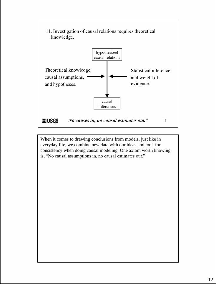
12

When it comes to drawing conclusions from models, just like in

everyday life, we combine new data with our ideas and look for

consistency when doing causal modeling. One axiom worth knowing

is, “No causal assumptions in, no causal estimates out.”

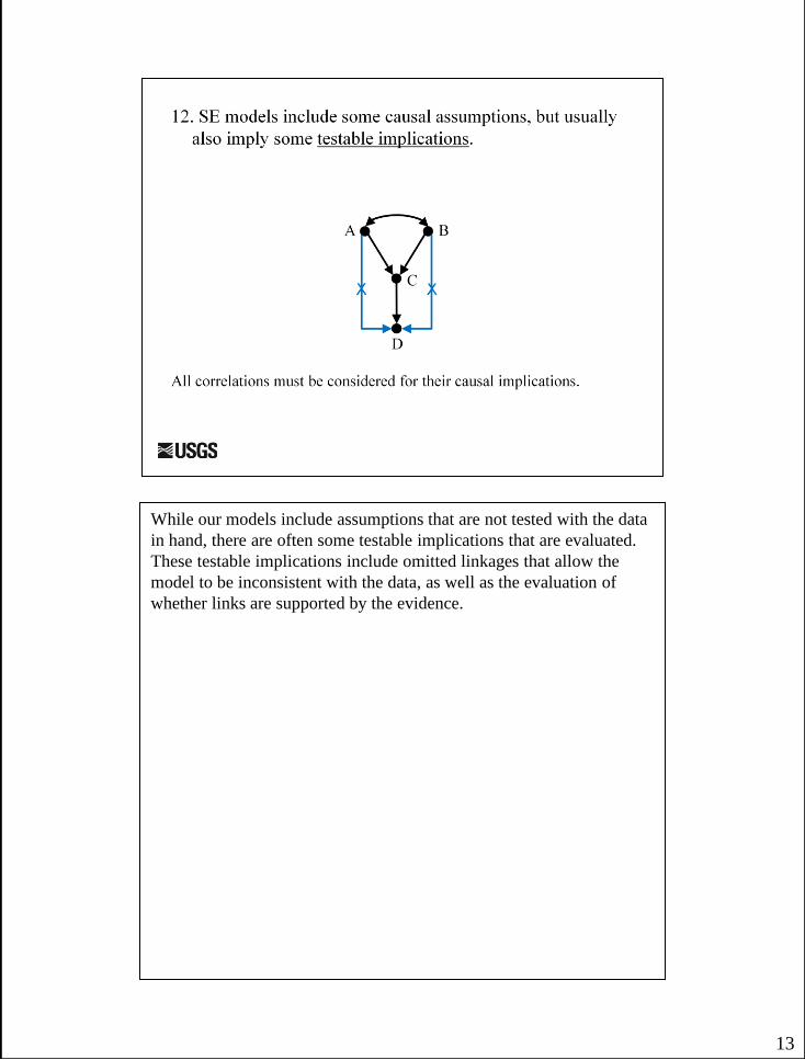
While our models include assumptions that are not tested with the data

in hand, there are often some testable implications that are evaluated.

These testable implications include omitted linkages that allow the

model to be inconsistent with the data, as well as the evaluation of

whether links are supported by the evidence.

13

14

Our intent with SEM is to build our knowledge as we go. Multiple,

overlapping investigations are required to build confidence in causal

interpretations. Our initial investigations are often exploratory or

“model-building” in that we use the data to build the model, thereby

not permitting an independent test of the model with the same data. We

have some ways of constraining just how exploratory our efforts are,

which will be introduced later. It may take several subsequent studies

before one graduates to true model-comparing or confirmatory studies.

15

In SEM, model failure often leads to a search for alternatives that

represents a new discovery of some missing component or need for an

alternative theory. There are now many examples of discovery through

SEM.

It is important to realize that SEM plays a particular role in the

scientific process. In the lower left-hand corner of this diagram, we see

that with new topics, where we do not have much understanding of

processes or much hard data, work tends to be descriptive. We often

aspire to reach the upper right corner of this box where we have strong

theoretical knowledge and well-described relations. SEM can help us

move across the page, but again, only plays a particular role in the

whole process.

16

SEM is also a work-flow process. This can be described in various

degrees of detail, but essentially we start with our objectives, ideas and

assumptions, add in data, and then proceed to develop and evaluate

specific models that give us both results and shed light on our

theoretical ideas and assumptions.

One implication of this diagram is that our ultimate test is nearly

always found in the next sample or the next study.

17

History has played a role in shaping the literature on SEM.

This diagram represents a citation map

(http://www.eigenfactor.org/map/maps.htm) showing the historical

flow of knowledge among disciplines.

It is important to realize how the flow of information, and especially

the lack of flow of information, shapes peoples’ perceptions of

quantitative methods.

Understanding the influence of history helps us to realize how many

important bodies of knowledge, such as that related to SEM, are

relevant to our science even if not currently part of the common body

of practice.

As the animation of this slide conveys, we have been working to bring

SEM into a more central position regarding the natural sciences and

also to bring in the latest advances in statistics and causal analysis

(from the field of artificial intelligence). Further, we have tried to

illustrate how SEM can be adapted to the needs of ecology and

evolutionary biology. This is described in our 2012 paper in Ecosphere

and in

Grace, J.B. 2015. Taking a systems approach to ecological systems.

Journal of Vegetation Science 26:1025-1027.

18

19

There are now a large number of resources related to SEM. Here are

just a few sources, the first two being books related to biological

systems. Kline’s books are a nice non-mathematical entry to the

subject. Bollen’s is a classic description of the modern method. Lee

illustrates the relation of Bayesian analysis to SEM. Hoyle has now

edited a volume with an extensive series of chapters on various SEM

topics. Shipley has a new edition of his book.

20

Two of our recent papers that cover broad fundamental treatments are

given here. The first of these discusses some fundamental principles

about the specification of models and how data are related to

theoretical ideas. The second of these represents our outlining of the

next (third) generation of SEM practice, in the form of guidelines.