this pdf is a selection from an out-of-print volume from ... · volume title: distribution of...

This PDF is a selection from an out-of-print volume from the National Bureau of Economic Research

Volume Title: Distribution of Economic Well-Being

Volume Author/Editor: F. Thomas Juster, ed.

Volume Publisher: NBER

Volume ISBN: 0-884-10478-8

Volume URL: http://www.nber.org/books/just77-1

Publication Date: 1977

Chapter Title: Black/White Male Earnings and Employment: 1960-70

Chapter Author: James P. Smith, Finis R. Welch

Chapter URL: http://www.nber.org/chapters/c4374

Chapter pages in book: (p. 233 - 302)

F

7JAMES P. Black/White Male

SMITH EarninRs andThe Rand L)

and Employment: 1960-70FINIS R.

WELCHUniversity of California

at Los Angeles andthe Rand Corporation

I. INTRODUCTION

Our goal in this paper is to examine several aspects of relative black/whitemale earnings between 1960 and 1970, using the 1960 and 1970 One-in-100 Samples of the United States Census of Population.'

There is absolutely no question that relative earnings of black Ameri-cans increased during the decade. There are, however, real questionsabout root causes of this change. Before summarizing our interpretationsof the evidence, we should note that although by historical standards thegain of the sixties is truly prodigious, the absolute magnitude of thechange is not overwhelming. In 1959, the average weekly earnings ofemployed black men came to 57 percent of the amount earned by

NOTE: We should like to thank Orley Ashenfelter, of Princeton University, and Rodney Smith, of theRand staff, for their comments on an early draft. We are grateful as well to research assistants FrankBerger, Richard Buddin, Anthony Casesse, Ann Dukes, and Iva Maclennan. The research was supportedby a contract from the U.S. Department of Labor to the Rand Corporation, and by a grant from the FordFoundation to the National Bureau of Economic Research. James P. Smith's work on the present reportbegan while he was a research associate at the National Bureau of Economic Research.

233

I -

I—

employed white men. The ratio had increased to 64 percent by1969—i.e., about 16 percent of the wage differential was bridged duringthe decade.

In accounting for growth in black/white wage ratios between 1960 and1970, the evidence is, first, that younger, more recent cohorts of blacksgained more than older cohorts. Second, within experience classes, risingschooling levels and migration have contributed to the relative increasesin black earnings. But the bulk of our evidence is that most of the gain ofthe sixties was broad-based. We did not find that gains were confinedeither to the highly schooled or to those employed by the governmentalsector.

Our descriptions of occupation and industry of employment alsoindicate that the gains accruing throughout the sixties were very broadlybased. There was marked black/white convergence of occupationaldistributions during the period, with the most pronounced change beingrealized by those blacks we estimate to have entered the work forcebetween 1960 and 1970.

Similarly, for the same group, we found—especially for those who hadattended college—that employment is moving from the traditionalgovernmental to the private sector. It also seems that there are quitestrong geographical patterns to changing black/white earnings ratios,with stronger gains registered in the South and North Central regionsthan in the Northeast and West.

Finally, in comparing earnings distributions, we find that there is morevariance among black men than among white men. This is true both ofobserved weekly wages and annual earnings and of our predictions ofthem based on least-squares regressions. Annual earnings variance isdominated by variance in weeks worked. But location of residence andyears of schooling also play an important role.

II. THE 1960s: THE HISTORICAL SEllINGAlthough our analysis in this paper relies on the 1960 and 1970 censuses,we think it is important first to place that decade in historical perspective.In many ways, the 1960s represented a sharp departure from the previouspattern of relative black/white incomes. It has also been claimed that thedata available for the 1970s already indicate that the relative economicposition of blacks has started to deteriorate from the position achieved inthe late sixties. It is our view that isolating the underlying causes of theimprovement during the sixties enables us to better assess whether the

234 Smith and Welch

1960s constituted a temporary aberration or whether the gains registeredduring that decade bode well for changes during the 1970s.

The paucity of good income data by race before 1940 is well known.Apparently, the best available statistics are those contained in thedecennial United States Census Reports. These reports give a colorbreakdown of the occupations of individuals for each Census year since1890. Gary Becker in his famous work on the economics of discrimina-tion used income weights from the 1940 Census to construct a time seriesindex of relative occupational position of blacks.2 Becker concludedthat the fifty-year period from 1890 to 1940 was best characterized asone in which the relative economic position of blacks remained remarka-bly stable. He stated more tentatively that the 1940s were a decade inwhich the black/white mean ratio finally began to rise. This latter findingwas confirmed in a more detailed and careful study of this period byJames Gwartney.3 Gwartney found that the nonwhite/white income ratiorose on average by 12 percent within regions during the 1940s.

Beginning in 1947, annual data for annual incomes are available in theCurrent Population Reports. Table 1 gives ratios of median incomes ofnonwhite to white families for each year from 1947 to Althoughthe post-World War II era is characterized by a definite upward drift inthe relative income of blacks, there were sharp cyclic swings. The pictureis not of a smooth trend in relative black incomes; rather, the evidence isof a relatively small trend factor imposed on an unstable, cyclicallysensitive, series. From 1947 into the mid-1950s, the ratio increased from.51 to .56. There followed a slight downward movement which continuedinto the early 1960s. Black/white incomes began to climb again after1963 with a jump between 1965 and 1966 and a steady rise between 1966and 1970. The dramatic increase between 1965 and 1966 is often used asevidence that the civil rights laws that just preceded this (1964—65) playeda large causative role in accounting for the recent improvement in theearnings of blacks. However, year to year changes in the series are oftenquite irregular, and we think that this inference is not warranted on thebasis of this evidence alone. For example, there are two other points(195 1—52 and 1958—59) where the increase in the black/white ratio isabout as large as the 196 5—66 change. In those years, there was, of course,no comparable legislation. This issue of the effect of this legislation isobviously important and we admittedly cannot adequately address it withcross-sectional data for only two years. However, our empirical evidencedoes cast some doubt on the role of this legislation. First, we are able toattribute the rise in the ratio to factors (schooling, migration) that movemore continuously over the period. Second, our single attempt tomeasure the influence of the governmental sector indicated that its effectwas probably small.

Black/White Male Earnings and EmpJoyment, 1960—70 235

TABLE 1 Ratio of Median Incomeof Black and White Families

YearRatio: Black and Other Races

to WhiteBlack toWhite

1974 0.62 0.581973 0.60 0.581972 0.62 0.591971 0.63 0.601970 0.64 0.61

1969 0.63 0.611968 0.63 0.601967 0.62 0.591966 0.60 0.581965 0.55 0.541964 0.56 0.541963 0.53 (NA)1962 0.53 (NA)1961 0.53 (NA)1960 0.55 (NA)1959 0.54 0.521958 0.51 (NA)1957 0.54 (NA)1956 0.53 (NA)1955 0.55 (NA)1954 0.56 (NA)1953 0.56 (NA)1952 0.57 (NA,)1951 0.53 (NA)1950 0.54 (NA)1949 0.51 (NA)1947 0.51 (NA)

SOURCE: U.S. Department of Commerce, Social and Economic StatisticsAdministration, Bureau of the Census.

NOTE: NA = not available. The ratio of black to white median familyincome first became available from this survey in 1964.

236 Smith and Welch

After 1970, and especially if the 1974 data are ignored, black/whiterelative wages began once again to decline. It is this most recent downturnthat has ignited the pessimism about the prospects for the future.

A more detailed representation of the recent period is given in Table 2which lists ratios of black/white income for males, females, and families

TABLE 2 Relative Black/White Median Income for AllPersons 14 Years and Older

Year

Males

All WorkersFull-YearWorkers

Females

Full-YearAll Workers Workers

FamilyIncome

1974 .61 .70 .90 .91 .581973 .60 .67 .90 .85 .581972 .61 .68 .93 .86 .591971 .60 .68 .88 .88 .601970 .59 .68 .91 .82 .611969 .58 .68 .84 .80 .611968 .59 .67 .79 .76 .601967 .57 .64 .78 .74 .59

I

SOURCE: Current Population Reports, Series P-60.

from 1967 to 1974. The general picture is a sharp rise in the late sixtiesfollowed by reasonably constant ratio during the seventies. In the last fewyears, there apparently was a slowdown in the rate of improvement forblacks. However, in view of the recessionary state of the economy, thisslowdown may not contradict our predictions of continued improvement.Business cycle downturns typically reduce black relative wages, so muchso, in fact, that the relatively constant ratio of black to white male income,in spite of the current recession, can be taken as evidence that longer-runforces are nullifying downward pressures. For example, a more optimisticview emerges in the relative wages of full-year workers (Table 2), where,presumably, the business cycle factors are better controlled.

At best, the patterns exhibited in Tables 1 and 2 are difficult tointerpret. Not only are they confounded by business cycles, but they failto correct for geographic location, age, schooling, and so on, factorswhich our analysis of the Census data shows are important determinantsof the relative earnings position of blacks. We find little in the publishedtables now available for the recent past that seriously alters our confi-dence in the conclusions we derive based on the 1960—70 comparisons.Although our study will deal exclusively with racial comparisons of males,brief mention should be made of the pattern of relative female wages by

Black/White Male Earnings and Employment, 1960—70 237

race. Both over the more recent period and over the entire postwarperiod, the gains achieved by black males relative to white males are smallcompared to those achieved by black women relative to white women.

III. BLACK/WHITE WAGE RATIOS:THE 1960 AND 1970 CENSUSESTable 3 illustrates the black/white ratios found in the U.S. Census. Fromamong those persons described, we analyze data for only those males withearnings in the two years in question, 1959 and 1969. Self-employed menare excluded, as are men with more than 40 years of imputed workexperience. Also excluded are those whose work experience is negative,when calculated as current age minus age of leaving school.5

Numbers reported are ratios of averages,6 i.e., they are average blackearnings or weekly wages relative to appropriate averages for whites. Thefirst column gives the black/white wage ratio for six experience classes in1970. The second column contains the same ratios for 1960, but thiscolumn is pushed down by two rows. Thus, the first entry, .5 10, isblack/white earnings for the 1—5-year experience cell in 1960; this cellhad 11—15 years of experience by 1970. The trend within an experiencecell as a new cohort enters can be read up the diagonal; the within-cohortlife cycle trends are illustrated across a row.

A number of patterns are apparent. First, the large earnings differen-tials that existed in 1960 were partly eroded between 1960 and 1970, but,as of 1970, differences remained large. Second, black/white earningsratios are highest for those we estimate as having entered the labormarket during the sixties, and they are higher for those entering between1965 and 1970 than for 1960—65 entrants. Among cohorts who were inthe labor market in 1960, with the exception of college graduates, we findthat by 1970 the relative position of blacks had improved only slightlyover 1960 levels. But, among the cohorts whose work experiencepredates 1960, the pattern exhibited for post-1960 entrants continues tohold: namely, that in comparison to whites, younger cohorts—morerecent entrants into the labor market—fare better than their earliercounterparts.

Third, the gains that occurred between 1960 and 1970 are broadlybased. With one exception, earnings ratios were higher in 1970 for everycohort than in This wage growth was fairly uniformly distributedacross experience and education cells for white males. This apparentgrowth neutrality for whites contrasts sharply with the patterns emergingamong blacks, where the extent of the gain is positively related to

238 Smith and Welch

TABLE 3 Black/White Earnings Ratios for Cohorts in 1960 and1970

Cohort Experienceas of 1970

Average AnnualEarnings Average Weekly Earnings

(Years Out of School) 1970 1960 1970 1960 1970/60

I. All School Completion Levels

1—5 .653 — .702 —

6—10 .648 — .677 —

11—15 .621 .510 .641 .568 .073

16—20 .601 .529 .618 .573 .04521—30 .594 .545 .616 .585 .03131—40 .604 .540 .620 .574 .046

II. Elementary School Graduates (8 Years Completed)

1—5 .835 — .8656—10 .779 — .802 — —

11—15 .708 .673 .737 .703 .034

16—20 .710 .688 .717 .713 .004

21—30 .749 .671 .763 .708 .05531—40 .721 .719 .740 .741 —.001

Ill. High School Graduates (12 Years Completed)

1—5 .775 .8066—10 .769 — .791 — —

11—15 .729 .654 .749 .714 .035

16—20 .731 .676 .750 .714 .036

21—30 .678 .655 .698 .685 .01331—40 .675 .623 .690 .648 .042

IV. College Graduates (16 Years Completed)

1—5 .716 — .775 —

6—10 .647 — .692 — —

11—15 .662 .618 .688 .655 .03316—20 .654 .559 .675 .582 .09321—30 .519 .446 .557 .470 .08731—40 .504 .389 .522 .421 .101

education level. The most spectacular improvement is undoubtedly thatof college-educated blacks, although the less skilled also gained relativeto whites. Some of the decline in growth rates by experience class in thecomplete black sample is due to shifting weights toward the less educated


in the older experience groups. The decline in relative black/white wagesas education increases becomes somewhat attenuated by 1970, for theolder experience groups.

An obvious source of gain between 1960 and 1970 is the improvementin the general level of economic activity that occurred during this period.The U.S. aggregate average unemployment rate, 5.5 percent in 1959, hadfallen to 3.5 percent by 1969. The penalties imposed by businesscontractions are not uniform over education, age, or racial groups, and asbusiness conditions improved over the decade, black earnings would haveincreased relative to white. Since it is widely acknowledged that theprincipal cyclical setbacks occur in employment levels rather than in wagestructures, the weekly wage comparisons in Table 3 are probably lesscontaminated by the business cycle than are annual incomecomparisons.8 The gains reported by blacks are smaller in the wage thanin the. annual earning comparisons.

Although there is a presumption in the literature known to us that wagerates are quite insensitive to cyclic vagaries, the empirical basis for thispresumption is unclear. A careful analysis of wage flexibility under cyclicfluctuations could go far in relieving our concern that the relative wagegains we document are merely a by-product of improving marketconditions.9 A number of the patterns we find seem to us inconsistentwith a purely business-cycle explanation. Other researchers have pro-vided convincing evidence that during recessionary periods those mostadversely affected are the less skilled (schooled),'° yet we find that thoseblacks who gained most in comparison to whites had the most schooling.Secondly, the change in the real characteristics of people (i.e., schoolingor location) observed during the decade would, in the absence of anybusiness-cycle trends, have led to an improvement in the relative incomeposition of blacks. It may be that part of the story of gain in relative blackearnings during the sixties is one of business cycles, but there seems tobe considerable room for the operation of other factors.

Cohort. Life Cycle, and Calendar Year Effects

One feature common to all cross-sectional comparisons of black/whiteearnings differences is that younger blacks fare better in comparison towhites than their older counterparts. This fact, in and of itself, isconsistent with extreme life cycle or cohort views (and, with a variety ofintermediate views) that have very different implications for the futurecourse of black/white differentials. Early theories of labor marketdiscrimination tended toward a life-cycle explanation, holding thaton-the-job black earnings increase less rapidly with work experience than

240 Smith and Welch

4

£

white earnings. These theories of "secondary" labor markets view labormarkets as stratified with some groups of workers being less upwardlymobile over their careers than others.

More recent comparisons have contrasted cross-sectional profilestaken at different points in time. If anything, these contrasts tend tosupport the extreme alternative to the life-cycle view, which is thatdifferences in the cross-section are indicative of cohort differences. Forexample, in Table 3 the evidence of gains between 1960 and 1970 forblacks relative to whites suggests that given individuals were relativelyunaffected. In contrast to the life-cycle view that predicts decliningrelative black wages between 1960 and 1970 within cohorts as workersaged ten years, the evidence is that wage ratios either remained constantor increased slightly. The aggregate gain stems mainly from changes incomposition.

The extreme life-cycle view offers no basis for predictions of futurepatterns of wage differentials. The cohort view, on the other hand, doesprovide a basis for predictions if the future course of differences amongcohorts conforms to the past. Suppose the evidence of the 1960—70Census contrasts between cohorts is maintained in examination of themore recent data, the natural extension is to ask why cohort experiencesseem so different over time.

There are a number of competing explanations to be scrutinized. Theseinclude questions of effects of modern antidiscriminatory legislation,trends in school quality and student achievement, as well as the possibilityof secular trends in (front-end) market discrimination per se. But,whatever the explanation, any potential to understand secular forces restsexclusively on an ability to distinguish secular trends from life-cycle andcyclical forces operating in the cross section.

In general, cross-sectional data cannot easily decompose relationshipsthat arise simply from maturation and those that are the result of a personof a particular age being the recipient of a variety of experiences that areunique to his generation. Each individual in a cross section is a member ofa distinct cohort at one point on his life-cycle path. If between-cohorteffects are important, the data must be adjusted before one has "pure"life-cycle elements. For example, the large secular increases in labor forceparticipation rates for married women suggest that cohort effects couldseriously contaminate cross-sectional labor supply studies. Similarly,improvement in school quality or home environment probably has led toa secular increase in the human capital stock of successive generationsand thus affects observed cross-sectional wage earnings profiles. Al-though cohort or generational effects are recognized as important sourcesof bias in cross-sectional data, most investigators assume simply thatempirically observed links between age and earning capacity are only the

Male Earnings and Employment, 1960—70 241

results of education and the associated skill acquisition process. Bycomparing cross sections at different points in time, the potential of dis-tinguishing between those effects is established. For example, Welch [16]found that within each of two cross sections (1960 Census and Survey ofEconomic Opportunity [SEO]), the income gain associated with an addedyear of schooling was lower for older workers. But, since these workerswere older, they had attended schools in periods in which schools werethemselves different, and had entered the labor market when the marketafforded different opportunities. By comparing persons of the samecohort (i.e., persons who had gone to similar schools and entered thelabor market at similar times) between these cross sections, drawn sevenyears apart, Welch found little evidence of attenuation over the life cyclein the return to schooling. Evidently, the attenuation observed withineach data set referred only to vintage or cohort effects, not to maturationper se.

Comparisons of successive cross sections give potential insight intodistinctions between experience and cohort effects, but these compari-sons are themselves confounded by calendar year effects. The problem isthat conditions of labor demand vary through time. If several cohortscould be observed throughout their careers under constant labor marketconditions, vintage and experience effects could more easily be distin-guished. But labor markets do not remain stable and prices (wage rates)reflect the market conditions associated with the calendar year in whichexchanges occur. Because of the identity that calendar year equalsvintage plus years in the labor market, it is never possible to separatelyidentify calendar year, experience, and vintage effects from time seriesobservations of cross sections without explicit parameterization of theseeffects. But, although the need for explicit parameterization is recognizedbecause several cross sections are observed simultaneously, and becausesome geographic detail is available to permit analysis of differencesbetween markets at a point in time, the constraints imposed by explicitparameterization are less bothersome than they would be with less data.For example, Rosen [12] has demonstrated that if one is willing to pursuethe theoretical implications of life-cycle human capital models in detail,then cohort and life-cycle effects are identified in a single crosssection—this, despite the one-to-one correspondence between age andcohort.

First, observe relative wage changes within cohorts. For those who hadentered the work force prior to 1960, black relative wages did not fallbetween 1960 and 1970." In either cross section (reading down acolumn), black/white wage ratios clearly deteriorate as experienceincreases or vintage is older, and the rate of decline is more pronounced athigher levels of school completion. But the within-cohort changes

242 Smith and Welch

A

between 1960 and 1970 are the mirror image of patterns exhibited in thecross section. Not only did the relative position of blacks improve as theyadded ten years of work experience, but this improvement was greatest athigher schooling levels. There are at least two extreme views forreconciling differences between cross-section and time-change patterns.One is that calendar year effects overwhelm the inherent tendenciesexhibited in the cross sections. A strong increase in demand for blackrelative to white labor, coupled with an increased demand for moreschooled labor, has this capability. In this view, unless the changes indemand patterns are persistent, more accurate projections of futurechanges should rely upon cross-sectional patterns. The other view is thatchanges within cohorts will persist and that the cross-sectional compari-sons are dominated by vintage effects.

Table 4 rearranges the data of relative weekly wages to facilitatevintage comparisons. In Table 4, the row comparisons hold workexperience constant and allow cohorts to change. The observed pattern isone of persistent cohort improvement in black/white earnings ratios withrelatively larger gains accruing to more schooled workers. The datareported in Tables 3 and 4 are not consistent with either a pure life-cycleor a vintage hypothesis. The pure life-cycle explanation predicts thatblack/white earnings ratios will decline throughout the work career.12Between 1960 and 1970 they clearly did not. The simplest vintage modelwould describe black/white wage ratios as functions only of cohort—oftime of entry into the job market. Other factors influencing income thatvary after a cohort enters the market would be race neutral so thatvariation in them would not affect wage ratios. If vintage effects reflectsecular change, either through rising relative quality of black labor ordeclining front-end labor market discrimination, then younger, morerecent cohorts of blacks would fare better in comparison to whites thanolder cohorts, but the differences existing within a given cohort in 1960would persist to 1970.

As far as career performance is concerned, it is difficult to conceive ofrelatively simple theories based either upon labor market discriminationor upon investments in skills acquired on the job that predict the observedpatterns of increases within cohorts in relative black earnings.13 Becauseof this, calendar year effects, i.e., changes in labor markets, emerge as alikely candidate for explaining the observed increases within cohorts. Weattribute the rising wages between cohorts to differential vintage effectsthat favor black males. Our "best guess" for rationalizing the proskill biasin rising black/white wage ratios within cohorts is that most of theexplanation lies in improving school quality. There is evidence thatnominal attributes such as days attended, school retardation rates,teacher educational levels, and teacher salaries have been improving


TABLE 4 Black/White Ratios of AverageWeekly Earnings by Years ofWork Experience, 1960 and 1970

Years of Average Weekly Earnings

Work Experience 1970 1960 1970/60

I. All School Completion Levels

1—5 .702 .568 .1346—10 .677 .573 .104

11—15 .641 .581 .06016—20 .618 .587 .03121—30 .616 .574 .04231—40 .620 .574 .046

II. Elementary School Graduates (8 Years Completed)

1—5 .865 .703 .1626—10 .802 .713 .089

11—15 .737 .724 .01316—20 .717 .696 .02121—30 .763 .741 .02231—40 .740 .710 .030

Ill. High School Graduates (12 Years Completed)

1—5 .806 .714 .0926—10 .791 .714 .077

11—15 .749 .682 .06716—20 .750 .690 .06021—30 .698 .648 .05031—40 .690 .590 .100

IV. College Graduates (16 Years Completed)

1—5 .775 .655 .1206—10 .692 .582 .110

11—15 .688 .582 .10616—20 .675 .517 .15821—30 .667 .421 .13631—40 .522 .422 .100

throughout most of this century for black students relative to whites. (SeeWelch [17].) Possibly more importantly, black students have beenswitching to integrated, traditionally white-dominated, schools—especially colleges.

244 Smith and Welch

1.

IV. ACCOUNTING FOR BLACK/WHITE INCOMEDIFFERENTIALS

To sort through the impact of various factors on earnings comparisons,we have estimated regression equations separately for blacks and whitesin 1960 and 1970. Our objective is to identify the most importantstructural differences in black and white wage equations and to account,insofar as possible, for wage differentials, based upon both observedcharacteristics and parameter differences. Individuals are partitionedaccording to our estimate of years of work experience. The independentor explanatory variables fall into four groups: (1) school completion; (2)geographic location; (3) government employment; and (4) years of workexperience.

There are two variables for school completed. The first ranges from 0 to12 and indicates years of elementary and secondary schooling. Thesecond measures years of postsecondary schooling. If a person reports apositive number of years of college, the grade-school variable is set equalto 12. This "spline" function is linearly segmented to permit slopecoefficients in the partial relation between (log) wages and years ofschooling to differ between the first 12 and succeeding years, but thelinear segments are constrained to join at 12 years. This specificationallowing for nonlinearities in the returns to schooling is useful, since itenables us to discover non-skill-neutral effects of governmental antidis-criminatory policies or improving school quality. Tests of equality for thetwo coefficients within experience classes show that equality can berejected in most cases.'4

Geographic location includes yes/no binary variables indicating resi-dence for the South, North Central and West regions. The omitted (base)class is the Northeastern region. Dummy variables are included if theindividual resides in a standard metropolitan statistical area (SMSA) andif the residence is within a central city of the SMSA, so that the omittedclass refers to residents of nonmetropolitan areas. A variable is alsoincluded indicating years in current residence, to approximate recency ofmigration.

A number of variables are added indicating whether the individual is anemployee of the federal government and whether he works in an industrythat is regulated by the federal government.'5 For those who neither workfor the federal government nor work in industries regulated by the federalgovernment, two additional variables are added. One represents pur-chases by the federal government as a fraction of value-added originatingin the industry. The other is similarly defined for purchases of state andlocal governments. With these variables, we attempt to identify wageeffects of governmental efforts to enforce antidiscriminatory legislation.


L

L

If black relative wages are affected by either working for, or beingregulated by, the federal government or are correlated with the govern-ment's share of industry product, an argument that this legislation had aneffect would seem stronger. Our presumption is that the federal govern-ment can have the most immediate and direct impact upon those firmsmost dependent on it.

The remaining class of variables describes a quadratic in years of workexperience. Although regressions are computed within experienceclasses, these variables are included to allow for correlations within classbetween wages and work experience. The estimated equations take theform

(1) y=x'bo+dix'ôi+d2x'82+did2x'812+u

where

ii if blackd1=1

10 otherwise

and(hf 1960

d2 =LØ otherwise

The dependent variable, y, is the logarithm (base e) of the weekly wage inconstant Consumer Price Index (CPI) dollars; x represents a vector of theindividual's characteristics as described in the above list of explanatoryvariables; b0, 81, and 612 are the associated parameter vectors; and u isthe omnipresent residual. Parameter vectors for individual groups in eachyear are

(white b0 (white b0+8219701 19601

tblack tblack b0+61+ô2+612

In this form, & summarizes parameter race effects and is simply thedifference between black and white parameters in 1970. Similarly, 62describes year effects and is the difference between 1960 and 1970parameters for whites. The interaction effect 612 allows the year differ-ences in parameters to vary by race or, equivalently, it allows racedifferences to vary by year. This fully interactive model yields exactly thesame ordinary least-squares (OLS) regression coefficients as would beobtained from the four separate race-by-year regressions. It does,however, give slightly different test statistics since in this pooled formthe estimate of residual variance is based on the sum of theresidual quadratics over the four groups, instead of being estimated

246 Smith and Welch

separately for each group.16 The advantage of this specification is thatit simplifies tests of linear hypotheses for race and year coefficientdifferences.

Estimates of equation 1 appear in Appendix Table A-2. Although thestatistics are interdependent, so that sequential tests risk incorrectinference, it is clear from inspection of the t-statistics for estimates of theparameters öi, and &12 that the fully interactive specification ofequation 1 is too general in the sense that it allows for parameterdifferences that apparently do not exist. It is, of course, true that byimposing parameter equality either between races, between years, orboth, estimation efficiency is gained.17 The impression that estimatesbased on equation 1 are not efficient is strengthened when they are usedto "account" for black/white earnings differentials. Too often we find aprediction of a small but statistically "significant" effect (of, as anexample, increasing black earnings relative to whites resulting fromdeclining differences in schooling) numerically swamped by a statistically"insignificant" effect (of, say, numerically large but insignificant yeardifferences in schooling coefficients).

Several of the variables suppressed in the constrained estimates arestatistically significant in the fully interactive model.'8 But in no case is avariable suppressed nor is race, year, or race-year interaction suppressedwhen its effect estimated in the fully interactive model is significant inmore than two of the six experience classes. Even though the imposedconstraints (among the six experience classes, there are 186 coefficientsdeleted from the fully interactive specification) delete variables that inthe main appear insignificant in the fully interactive model, the joint testfor significance clearly rejects the null hypothesis.'9 Although thecomputed F-statistics for the classes are not large by conventionalstandards (ranging from 1.2 to 2.6), the number of observations is simplytoo large to permit acceptance of the implied null hypotheses. Thisproblem of an inability to reject hypotheses is common to large samplesand has resulted in a number of attempts to weaken test criteria.20 For ourpurposes, we note only that the constrained estimators are more efficientand whatever biases they imply are simply biases that we feel arenecessary to clarify our estimates of factors contributing to increasingblack/white ratios.

ResultsThe summary of our results and imposed coefficient constraints (sup-pressed variables) is:


-J

1. Education—The Returns to Schooling

Income differences associated with schooling may vary by school level, anindividual's cohort or vintage, his position in the life cycle, the generalstate of the economy, and perhaps even personal characteristics, likeone's race or sex. It is important that evidence of the underlying nature ofobserved variation be provided since implications of the several potentialsources of variance differ dramatically, not only for purposes of describ-ing the likely course of future black/white wage comparisons, but foreducational policy as well. For example, the well known cross-sectionaldeterioration of the returns to schooling with increasing age may be alife-cycle phenomenon that results from a negative correlation betweenthe proportion of income devoted to two types of investment (schoolingand on-the-job training) or it may reflect improvement in the schoolingquality and home environments of new, more recent cohorts.

For the grade-school variables, the full interactive estimates suggeststatistically "significant"21 race interaction for all six experience classes,with returns to grade school for blacks being lower than for whites.Based on our estimates, the marginal returns to postsecondary schoolingare actually higher for blacks in the 1—5-year experience interval. We findno statistically significant difference by race in the college returns in theother experience intervals. If school systems are not an effective means ofincreasing black incomes, it is clear that the problem lies at the elemen-tary and secondary levels.

Both the unconstrained and constrained estimates of returns to gradeschooling show a clear life-cycle pattern, with schooling being a lessimportant discriminator of earnings for older, more experienced workers.In contrast, the estimated returns to college also indicate a declininglife-cycle profile, but most of the change occurs between the 1—5 and 6—10classes, and thereafter the descent is slow relative to the changing returnsobserved for grade schooling. We consider this an important finding andworth additional research. A number of hypotheses are consistent withthis. Quite probably the skills acquired in college are more complemen-tary with job experience than are skills acquired in grade school. Rates ofobsolescence of knowledge could differ by skill level with less rapid ratesat higher skill levels.22

Concentrating on the coefficients that measure secular movements, wefound no trend in the returns to grade school for either race between 1960and 1970. The full interaction estimates of wage returns to collegeindicate year interaction, with returns lower in 1960 than in 1970 in allclasses. The associated t-ratios exceed 2.0 in absolute value in threeexperience intervals. This rise in returns to college in 1970 may besurprising to many. It was thought that the middle sixties could have been

24.8 Smith and Welch

a critical turning point in the market for educated people. The compara-tively well-educated postwar baby-boom cohorts were beginning in thelast half of the decade to enter the labor market. This historically uniquelarge increase in the relative supply of educated men combined withsome factors reducing the relative demand for skilled labor could havebegun the long-awaited decline in the returns to schooling. Using theCensus data, this decline in the skill differential had not occurred by 1970.Based on results in the fully interactive model, we impose the followingconstraints: for grade-school coefficients, all year and race-yearinteractions are suppressed; for college coefficients, all race-yearinteractions and all race interactions except the 1—5 experience group aresuppressed.

This last finding serves as a benchmark for an important paper byRichard Freeman [4] whose observations are from the published sum-mary tables from the CPS. He claims that by the mid-seventies careerpaths for college graduates were substantially depressed relative to thepast (notably, 1969). His point is illustrated in Table 5. Clearly, on thebasis of these published tables, returns to recent college graduates havedeclined. Although Freeman argues that this observed change is (1)severe and (2) permanent, there is reason for skepticism. Freeman'sanalysis is restricted to the 1967—73 period and uses only the boundaryyears for calculations of change. Clearly, using these two years maximizesthe decline in the relative income of college graduates. If, for example,1967 is used as the base, the overall decline is much less pronounced. Infact, with an exception for the youngest age group, there is little evidenceof any change at all.

The fact that cyclical factors may explain declining relative earnings ofthe young is added reason for skepticism about the permanency of "thedeclining economic value of higher education." It is generally argued thatcyclical downturns offer a relative advantage to more skilled workers.This argument is founded on the presumption of "quasi-fixity" orspecificity of training on the job being positively correlated with levels ofschooling. If it is, the argument goes that the more skilled workers will bestockpiled or hoarded by finns during periods of reduced labor demandwith an eye toward recouping any short-run losses during future expan-sionary periods. The empirical basis for this argument (see Oi [10] andRosen [11]) is strong, and if it is correct, its counterpart is that if a firm is inthe process of hoarding, i.e., underutilizing, its skilled manpower, itsurely will not be simultaneously hiring new (young) skilled laborers.

If the theory predicts that skilled workers with job seniority are lessvulnerable to cyclic vagaries than others, it must also predict that newentrants to the skilled work force are more vulnerable than others. Thelarge influx of college graduates that coincided with the recent cyclical


_1

TABLE 5 Recent Returns to Education: Mean Income Ratios

—1967— —1969— —1971— —1973—Age HI/EL0 C/HIb HI/EL C/HI HI/EL C/HI HI/EL C/HI

Year-Round Full-Time Workers

Male:All Races

25—34 1.34 1.32 1.22 1.39 1.33 1.29 1.30 1.2335—44 1.38 1.50 1.38 1.54 1.32 1.50 1.21 1.4845—54 1.31 1.50 1.32 1.65 1.30 1.64 1.37 1.5655—64 1.26 1.49 1.32 1.66 1.36 1.48 1.27 1.6165+ 1.12 1.72 1.25 1.42 1.31 — 1.32 1.37

25+ 1.27 1.44 1.29 1.53 1.28 1.46 1.24 1.40

Female:All Races

25—34 1.40 1.36 1.45 1.42 1.42 1.38 — 1.3435—44 1.27 1.64 1.29 1.31 1.31 1.54 1.31 1.4945—54 1.20 1.48 1.25 1.43 1.35 1.45 1.27 1.3755—64 1.30 1.40 1.35 1.50 1.38 1.56 1.33 1.3965+ 1.43 — 1.27 — 1.44 — — —

25+ 1.26 1.46 1.28 1.40 1.34 1.44 1.26 1.36

All Workers

Male:All Races

25—34 1.38 1.33 1.24 1.33 1.42 1.27 1.37 1.1935—44 1.37 1.54 1.41 1.87 1.36 1.55 1.27 1.5245—54 1.35 1.53 1.36 1.64 1.36 1.66 1.37 1.5655—64 1.33 1.55 1.39 1.68 1.43 1.59 1.36 1.5765+ 1.34 1.76 1.46 1.58 1.44 1.64 1.36 1.69

25+ 1.47 1.47 1.52 1.50 1.53 1.48 1.49 1.41

Female:All Races

25—34 1.22 1.42 1.32 1.54 1.40 1.51 1.35 1.4535—44 1.30 1.47 1.26 1.37 1.26 1.47 1.33 1.3545—54 1.33 1.54 1.41 1.54 1.44 1.54 1.45 1.4555—64 1.51 1.58 1.58 1.69 1.57 1.71 1.58 1.6665+ 1.61 1.90 1.70 1.45 1.49 1.55 1.47 1.43

25+ 1.58 1.51 1.60 1.50 1.61 1.50 1.60 1.42

0H1/EL is the ratio of high school to elementary.bC/HI is the ratio of college graduates to high school.

250 Smith and Welch

r

downturn seems to have met a predictable fate. Whether their reducedrelative wage will persist is uncertain, but the recent experience is adubious basis for extreme pessimism.

The available evidence is that schooling, especially college, offersearned rates of return to recent cohorts of blacks that are comparablewith those earned by whites. This appears not to have been true of earliercohorts of blacks for whom returns to schooling were sharply lower.

The improved prospects of schooling as a vehicle for increasing blackincome has had its consequences on school enrollment rates. Accordingto Table 6A there has been a remarkable upsurge since 1965 in schoolattendance for blacks at both the preelementary and postsecondarylevels. College enrollments increased 55 percent, while enrollment ratesfor whites rose by only 15 percent between 1965 and 1974. Perhaps themost dramatic evidence of this shift is illustrated in Table 6B. During the1970—74 period, the proportion of black males enrolled in college rosefrom 16 to 20 percent, while the corresponding proportion for whitemales fell from 34 to 28 percent.

The historical record suggests that convergent schooling levels havebeen an important source of increasing income panty for blacks. Whetherthis is in fact true, requires accurate estimates of the effects of schoolingon earnings. Whether schooling will continue to be an important avenueof social and economic mobility depends very much on the future courseof the income returns to schooling. If the economic value of highereducation is falling, it is important that this evidence be presented.Evidence which "goes the other way" is equally important. This evidencecannot be obtained from summary tabulations without corrections forconfounding factors. To interpret the recent experience, it is especially

Percent Enrolled in School by1974

Age: 1965, 1970, and

Age 1965

Black

1970 1974 1965

White

1970 1974

3 and 4 years 12' 23 29 10 20 29

5 years 59 72 87 72 81 90

6 to 15 years 99 99 99 99 99 99

16 and 17 years 84 86 87 88 91 88

18 and 19 years 40 40 44 47 49 43

20 to 24 years 9 14 17 20 23 22

SOURCE: U.S. Department of Commerce, Social and Economic Statistics Administration, Bureau of theCensus.

'Includes persons of "other" races.


TABLE 6A

TABLE 6B College Enrollment of Persons 18 to 24 YearsOld by Sex: 1970 and 1974(In thousands)

Sex and College Enrollment

—Bla1970

ck— —W1974 1970

hite—1974

Both Sexes

Total persons, 18 to 24 years 2,692 3,105 19,608 22,141Number enrolled in college 416 555 5,305 5,589Percent of total 15 18 27 25

Male


Female


SOURCE: U.S. Department of Commerce, Social and Economic Statistica Administration, Bureau ofthe Census.

important that evidence be obtained of interdependencies between ageprofiles of income returns to schooling and general levels of economicactivity.

2. Geographic LocationEven after adjusting for education, experience, and government employ-ment, regional differences in black/white earnings persist. The South isdistinguished by low wages for both blacks and whites. Further, com-pared to the Northeast, black/white earnings ratios are consistently lowerin the South. In 1970, white male wages are 8 to 13 percent lower, whileblack wages in the South range from 15 to 30 percent below those forblacks in the Northeast. These black/white Southern wage ratios declinerapidly with experience. As we mentioned earlier, declining wage ratioswith experience can be attributed either to cohort or life-cycle factors,and the South may differ from the rest of the country in both. Althoughwe rejected year interaction for all experience classes, race-year interac-tion existed for the three classes with up to 15 years of experience. An

252 Smith and Welch

I 4

interpretation that appeals to us is that there are differential vintageeffects favoring black Southern males for the post-World War II labormarket entrants. An alternative explanation is that the presumably moreintense discrimination in the South against blacks takes the form ofrestricting blacks from occupations that have rising career wage profiles.

Disparities among the other three regions excluding the South are lesspronounced. In the North Central region, for all classes with at least 10years of experience, blacks and whites receive wages 3 to 5 percent higherthan the Northeast benchmark. For these experience classes, the increaseis independent of race and year, so that in our constrained estimates wesuppress all race, year, and race-year interaction. In the North Centralregion, for workers with less than ten years experience, black wages werehigher in 1970 than for blacks in the Northeast, but no white wagedifferentials existed between those two regions. Apparently, black/whiteearnings ratios increased in both the South and North Central regionsrelative to other areas. For these less experienced North Central workers,the main coefficient and year interaction is suppressed, but race andrace-year interaction is permitted. The main coefficient for the Westis suppressed for those with more than 15 years of experience.The estimates suggest that earnings of all persons in 'the West fell from1.4 to 10 percent between 1960 and 1970, relative to wages in otherregions.

3. Government EmploymentAfter adjusting for schooling, experience, and location, employees of thefederal government in 1970 have higher wages than others—a differen-tial of 5 to 16 percent for whites and 15 to 30 percent for blacks. Thispremium for blacks over whites represented a 10 percent decline from aneven higher differential in 1960. In fact, the black/white wage ratio didnot change for federal employees between 1960 and 1970. The declinerelative to the private sector simply notes the approximately 10 percentincrease that occurred in the private sector. The variable for directemployment by the federal government is retained with race andrace-year interaction, but year interaction is omitted.

Employees of regulated industries earn 8 to 16 percent more thanthose in the rest of the private sector. Employment in industries regulatedby the federal government is included without race, year, or race-yearinteraction. Between 1960 and 1970, black employment shares of theseindustries increased, so that regulated industries contributed slightly torising earnings ratios. The regression coefficients for the shares ofindustrial products purchased by the government are very large. Theypredict for whites that earnings in this form of indirect government

Black/White Male Earnings and Employment. 1960—70 253

employment exceed those of the private sector by one-third to one-half.Since we have similar results for another independently drawn sample,23we feel that the estimate cannot be reasonably construed as resultingeither from purely random fluctuations or from peculiarities of thesesamples. Instead, we think they signal real industrial wage differences.We will not speculate here about causes of these differentials, but willnote that we feel that industrial wage differentials represent a fruitfularea of research about which too little is currently known.

Wage differentials between white employees of federal contractors andthose in the private sector are also large, as are the estimated discrepan-cies in black/white wage ratios between this and other sectors. Wherewhites fare well, blacks appear to do even better. This, of course, is whatwe would expect from "affirmative action." The rub is that in theseindustries implied black/white earnings ratios fall at an average annualrate of 3 to 6 percent per year relative to the private sector (which wasrising at about 1 percent per year). We cannot think of a simple andsuitable explanation for this decline. Federal shares of industry valueadded is retained with year interaction being suppressed. All interactionis suppressed for state and local governments' shares of industry product.

4. ExperienceAll interaction is suppressed for the variables indicating years of workexperience and its square.

Accounting for Black/White Earnings Differentials

In this section, we present our attempts to account for the black/whitewage ratio as it existed in 1970, and for changes in the ratio between 1960 C

and 1970. Groups are specified separately by race, year, and workexperience. For each (the logarithm of) weekly wages is taken as a linearfunction of the schooling, location, government employment, and experi-ence variables described earlier so that (the logarithm of) the black/whitewage ratio is the difference in the linear expressions and (the logarithmof) the change in the ratio is the difference in differences. For the ratio, R,we have

(2)

and

(3) In R = (Yi Y2)(Y3Y4)

254 Smith and Welch

I

I

where x refers to characteristics affecting earnings with associatedparameter vectors fi. The subscripts are: 1 blacks, 1970; 2 = whites,1970; 3 = blacks, 1960; and 4 = whites, 1960. We are concerned withaverages and assume that the x's refer to mean vectors for the respectivegroups. The estimated equations include intercepts, so that estimates areforced through the geometric mean for each group. Henceforth, we referto OLS regression parameter estimates rather than their conceptualcounterparts and omit reference to residual means, which are constrainedto zero. In comparing equation 1 to equations 2 and 3 note that

b0=f32

131132

62 = 134—132

812 =(133—131)—62

Accordingly, equation 2 is rewritten as:

(2.1)

(2.ii) +x1ô1

where the first term on the right-hand side is the main effect ofblack/white mean characteristic differences, weighted by white parame-ter values, and the second term (2.ii) adjusts for race parameterinteraction.24 Equation 3 is rewritten as

(3.1) In = [(x1 —x2)'— (x3 —x4)'Jbo

(3.11) +(x1 —x3)'61

(3.jjj) — (x3 —x4)'ô2

(3iv) —4812

where the main effects of 1960—70 changes in characteristic differences,evaluated at 1970 white parameter values, is measured by the first term.The second adjusts for race interaction, the third for year interaction, andthe fourth for race-year interaction.

In this form, note that the intercept race-year interaction coefficientestimates (with opposite sign) the growth in the black/white wage rationot explained by changes in characteristics included as explanatoryvariables. This unexplained residual represents our estimate of skill-neutral relative racial vintage effects. One can only speculate, as we shall,about the factors contributing to the black relative income growthcontained in the intercept. It is important, however, that if vintage effectsexist, they are obvious candidates for time-related shifts in the interceptsof these wage-determining equations.


Similarly, notice that the year interaction intercept coefficient esti-mates time-related shifts in real wages of whites. Our estimates amongthe six experience classes show average annual growth for wages of whitesranging from 2.3 to 2.8 percent. We think these numbers agree withconsensus estimates of real wage changes over the period. Similarly, weestimate that neutral wage growth for blacks exceeded that of whites byaverage annual differentials ranging from 0.62 to 1.08 percent. Theseestimates are summarized in Table 7, which also contains observedaverage annual increments in annual earnings and weekly wages forwhites and for black/white ratios.

TABLE 7 Observed Growth in Earnings and Black/WhiteRatios with Residuals from RegressionAccounting for Change, 1960—70

Average Annual Yea rs of Work Experience

Percentage Change 1—5 6—10 11—15 16—20 21—30 31—40

Annual Earnings (Observed Increase)

WhitesBlack/White Ratio

3.00 2.78 2.99 3.06 3.21 3.152.67 2.25 1.75 1.29 1.09 1.09

Weekly Wages (Observed Increase)

WhitesBlack/White Ratio

2.49 2.41 2.66 . 2.76 2.74 2.642.25 1.73 1.06 0.75 0.70 0.68

Weekly Wages (Accounting Residual—Standard Errors in Parentheses)

Whites

BlackfWhite Ratio

2.81 2.60(.23) (.19)0.96 0.62(.39) (.31)

Table 8 summarizes the spline function estimates of returns to gradeschool and college. These coefficients are given special attention becausedifferences in school completion levels seem an important source ofblack/white wage differentials and because growth in black schoolinglevels relative to whites appears to be an important source of growth inrelative black earnings. Locational effects seem even more importantthan schooling in the accounting, but the pattern of change vis-à-vislocation seems more a result of black/white coefficient differences and oftime-related changes in coefficients than a gain due to migration per Se. Inany case, black/white earning differentials exist in all regions, and the

256 Smith and Welch

2.41(.18)0.75(.24)

2.30(.18)1.08(.20)

2.53(.13)0.81(.15)

2.57(.15)1.02(.18)

L

TABLE 8 Regression Coefficients for Years ofSchooling by Work Experience Classes(t-statlstlcs in parentheses)

Years of Interaction

Experience White, 1970 Race Year Race-Year

Fully Interactive Model: Grade Schooling Coefficients

.138(18.9).107

(21.4).067

(14.6).061

(13.9).058

(19.9).047

(15.3)

—.046

(4.8)—.015

(2.3)—.013

(2.3)—.016

(2.8)—.028

(7.3)—.019

(4.6)

.012(1.1)

—.012(1.7).004(0.7)

—.002(0.4).001(0.3).007(1.5)

Fully Interactive Model: College Coefficients

.123(25.0).088

(20.9).090

(21.9).088

(19.6).076

(20.2).074

(13.3)

.039(3.8).012(1.4).007(0.9)

—.001(0.1).009(1.2).001(0.1)

—.024(3.1)

—.008(1.2)

—.011(1.6)

—.020(2.8)

—.004(0.6)

—.025(2.6)

6—10

11—15

16—20

2 1—30

31—40

1—5

6—10

11—15

16—20

21—30

31-40

—.005(0.3)

—.011

(1.2)—.004

(0.6)—.004

(0.6).001(0.1)

—.011(1.9)

—.006(0.3).008(0.6)

—.011

(0.9)—.013

(0.9)—.021

(1.7)—.002

(0.1)

Constrained Estimates: Grade Schooling Coefficients

6—10

11—15

16—20

2 1—30

.143(27.6).101

(28.3).069

(22.7).062

(22.1).058

(29.4)

—.046

(6.9)—.018

(4.0)—.015

(4.0)—.019

(5.2)—.027(10.7)


1—5

1—5

—J

TABLE 8 (concluded)

Years of InteractionExperience White, 1970 Race Year Race-Year

Constrained Estimates: Grade Schooling Coefficients

31—40

1—5

6—10

11—15

16—20

2 1—30

31—40

.049(22.5)

—.023(8.3)

Constrained Estimates: College Coefficients

.124(26.9).093

(26.0).092

(27.0).088

(23.8).077

(24.4).074

(15.2)

.034(4.2)

—.024(3.8)

—.011(2.0)

— —.013(2.5)

— .023(4.0)

— —.008(1.5)

— —.024(2.9)

income potential to migration is limited. In contrast, patterns of schoolingcoefficients and of changing race differences in schooling levels suggestthat schooling continues to offer real potential for black income growth.

Table 9 summarizes our regression estimates of factors contributing toblack/white earnings differentials as of 1970. In all cases, schoolingaccounts for a much larger part of the black/white earnings differentialthan does location, government employment, or work experience.Except for the first experience class, the schooling effect is approximatelyequally divided between the main effect of lower average completionlevels and the effect of lower schooling coefficients. For example, in theclass with 1 to 5 years of work experience, the coefficient, —.174, for themain effect of schooling differences indicates that when weighted byschooling coefficients for whites, the black/white difference in averageschooling is large enough to predict black wages (approximately) 17.4percent below whites. The —.49 is an adjustment for the lower returnsblacks gain for schooling. This rather large racial interaction effect in1970 must be considered quite tentative, since we have found it sensitiveto model specification.25 For the other experience intervals, the raceinteraction term reflects a lower return to black elementary and secon-dary schooling.

258 Smith and Welch

I

TABLE 9 Black/White Weekly Wage Ratios: ObservedRatios with Regression Accounting forDifferentials, 1970

Variable Main Effects Race Interaction Total

Class I: 1—5 Years of Work Experience8

Accounting summary:Years of schooling —.175 —.491 —.666Geographic location —.052 .077 .025Government employment

(direct; regulated andsupply industries) —.011 .013 .002

Experience correction .010 — .010Total —.228 —.401 —.629Residual .204

Class II: 6—10 Years of Work Experienceb

Accounting summary:Schooling —.137 —.186 —.323Location —.039 .031 —.008Government —.010 .005 —.005Experience .003 — .003

Total —.183 —.150 —.333Residual = —.107

Class III: 11—15 Years of Work Experience'

Accounting summary:Schooling —.123 —.154 —.277Location —.037 —.008 —.045Government —.011 .008 —.003Experience .001 .001

Total —.170 —.154 —.324Residual = —.157

Class IV: 16—20 Years of Work Experienced

Accounting summary:Schooling —.127 —.185 —.312Location —.038 —.027 —.065Government —.009 .019 .010Experience .000 — .000

Total —.174 —.193 —.367Residual = —.123


TABLE 9 (concluded)

Variable Main Effects Race Interaction Total

Class V: 21—30 Years of Work Experience0

Accounting summary:Schooling —.131 —.242 —.373Location —.029 —.068 —.097Government —.008 .020 .012Experience .000 — .000

Total —.168 —.290 — .458

Residual = —.046

Class VI: 31—40 Years of Work Experience'

Accounting summary:Schooling —.139 —.178 —.317Location —.033 —.049 —.082Government —.006 .030 .024Experience —.001 — —.001

Total —.179 —.197 —.376Residual = —.137

8Log (base e) of observed weekly wage ratio —.422(base e) of observed weekly wage ratio —.439(base e) of observed weekly wage ratio = —.481

dLog (base e) of observed weekly wage ratio = —.4910Log (base e) of observed weekly wage ratio = —.503'Log (base e) of observed weekly wage ratio = —.5 12

Three characteristics—Southern, central city, and metropolitanresident—dominate the geographic location accounting in explainingblack/white 1970 wage ratios. The Southern black wages are the singlemost important locational source of low black relative wages. We findthat Southern residence reduces the black/white wage ratio from 3 to 13percent. This differential grows monotonically with experience andreflects primarily differential coefficients rather than characteristics. Thecentral city variables increase relative black wages by approximately 6percent. The negative effect of fewer blacks living in central cities isoverwhelmed by the positive differential favoring blacks. The metropoli-tan variable leads to a 2 to 3 percent reduction in the relative black wage.The net effect of all the locational variables is small in the first twoexperience intervals. In the 11 + experience groups, black wages rangefrom 4 to 9 percent lower because of their locational distribution. Thedetrimental effect of predominantly Southern residence is simply muchmore pronounced for older workers.

260 Smith and Welch

r

The systematic earnings determinants with adjustments for race coeffi-cient interaction predict a black/white wage ratio below the one actuallyobserved for those with 1 to 5 years of experience. The discrepancybetween predicted and observed ratios is absorbed by intercept-raceinteraction denoted as the residual in Table 9. For all other experienceclasses the intercept interaction term is negative, so that the regressionsunderaccount for black/white wage differences, i.e., relative to whitesblacks earn less on the average than predicted by the regression equa-tions.

Table 10 contains our summary accounting for 1960—70 changes inwage ratios. Here, patterns are confounded by interaction. The maineffects, those based on changes in characteristic differences (at 1970white coefficient values) consistently predict rapidly rising wage ratios,with schooling playing the leading role. Thereafter, the lower coefficientson black grade schooling and the 1970 increase in returns to college(where black/white completion differentials are large) take their toll. Themost rapid increases in schooling occurred in the earlier decades of thiscentury, but these are still sizable increases, especially for blacks.26

Surprisingly, vintage effects—time-based coefficient changes—are evi-dent only for the income returns to college. Considerable data (Welch[15], [16], [17]) exist to suggest that the nominal characteristics ofschools which are presumably indicative of "quality" have progressedsteadily for whites and even more rapidly for blacks. There is in fact nostrong a priori reason to assume that increased quality of schooling willnecessarily alter the semilogarithmic coefficients of wages on schooling.First, under stationary labor market conditions, the model of investmentin human capital presented by Yoram Ben-Porath [3] clearly makes thispoint. Second, as markets adjust in response to increased skills associatedwith increased schooling quality, the returns to education may decline.Finally, the firm-specific theories of investments in human capital on thejob and the associated quasi-fixity hypotheses27 all predict countercyclicmovements in returns to schooling, and it is at least within the realm ofimagination that the relatively "tighter" labor markets of 1969 incomparison to those of 1959 nullified longer-term tendencies.

Nonetheless, full skill-neutrality of vintage effects derived from secularimprovement in quality of schooling is not intuitively obvious and we—atleast one of us, who is on record as predicting the opposite result[16]—are surprised by these estimates, at least for grade-school coeffi-cients. Estimates for college do show time-related increases in returnsthat are not easily explained without reference to vintage hypotheses orto changing patterns of colleges attended by blacks.

Locational effects for those with the least experience are dominated byrace-year interaction—a result of rising black earnings ratios in the South


TABLE 10 Average Annual Percentage Increase in Black!White Weekly Wage Ratios, 1960—70:Accounting According to RegressionEstimates by Work Experience Class

Intera ction Effects

Main RacexVariable Effects Race Year Year Total

Class I: 1—5 Years of Work Experience'

Accounting summary:Years of schooling .91 —.40 —.22 — .29Geographic location —.00 .11 —.02 1.02 1.11Experience correction .03 — — — .03

Subtotal .94 —.29 —.24 1.02 1.43Government employment

(direct; regulated andsupply industries) .12 .03 — —.31 —.16

Total 1.06 —.26 —.24 .71 1.27Residual = .96

Class II: 6—10 Years of Work Experienceb

Accounting summary:Schooling .76 —.19 —.07 — .50Location .10 .12 .05 .50 .77Experience .01 — — — .01

Subtotal .87 —.07 —.02 .50 1.28Government .05 —.01 — —.21 —.17

Total .92 —.08 —.02 .29 1.11Residual = .62

Class III: 11—15 Years of Work Experiencec

Accounting summary:Schooling .40 —.20 —.07 — .13Location .03 .10 .05 .23 .41Experience .01 — — — .01

Subtotal .44 —.10 —.02 .23 .55Government —.01 —.01 — —.23 —.25

Total .43 —.11 —.02 .00 .30Residual = .75

Class IV: 16—20 Years of Work Experienced

Accounting summary:Schooling .23 —.26 —.09 — —.12Location .04 .14 —.04 — .14

262 Smith and Welch

I.

I

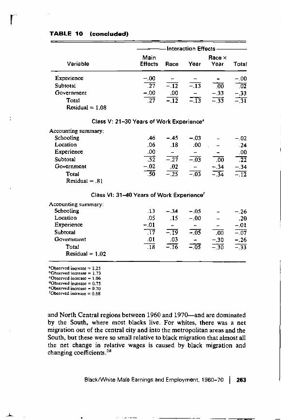
TABLE 10 (concluded)

Interaction Effe

MainVariable Effects Race Year

cts

Race xYear Total

Experience —.00 — —

Subtotal .27 —.12 —.13—

.00—.00

.02Government —.00 .00 — —.33 —.33

Total .27 —.12 —.13 —.33 —.31Residual = 1.08

Class V: 21—30 Years of Work Experiencee

Accounting summary:Schooling .46 —.45 —.03 — —02Location .06 .18 .00 — .24Experience .00 — — — .00Subtotal .52 —.27 —.03 .00 .22Government —.02 .02 —

Total .50 —.25 —.03—.34—.34

—.34—.12

Residual = .81

Class VI: 31—40 Years of Work Experience'

Accounting summary:Schooling .13 —.34 —.05 — —.26Location .05 .15 —.00 — .20Experience —.01 — —

Subtotal .17 —.19 —.05—

.00

—.01—.07

Government .01 .03 — —.30 —.26Total .18 —.16 —.05 —.30 —.33Residual = 1.02

aObserved increase = 2.25bObserved increase 1.73CObserved increase 1.06dObserved increase = 0.75CObserved increase = 0.70'Observed increase = 0.68

and North Central regions between 1960 and 1970—and are dominatedby the South, where most blacks live. For whites, there was a netmigration out of the central city and into the metropolitan areas and theSouth, but these were so small relative to black migration that almost allthe net change in relative wages is caused by black migration andchanging coefficients.28


r

Table 11 summarizes these coefficients, which are our "other thingsequal" estimates of increases in the earnings ratio observed between1960 and 1970 in the South and North Central regions, relative to theNortheastern base.

TABLE 11 Race and Race-Year Interaction Coefficientsfor the South and North Central Regions(t-statistics in

Years ofExperience Race

South

Race-year

—NorthRace

Central—Race-Year

1—5 —.017(0.5)

.152(3.6)

.075(2.4)

.082(1.7)

6—10 —.097(3.7)

.045(1.4)

.141(5.6)

.123(3.2)

11—15 —.158

(6.9).044(1.7)

—

—

—

—

aThe sign of the race-year interaction is from the form described in equation 1. (Race-regioninteraction coefficients are included for reference.)

Between 1960 and 1970 our estimate is that the black/white wage ratioin the South increased by 15.2 percent for those entering the labor marketin 1965—69, in comparison to the wage experienced in 1959 by those whoentered between 1955 and 1959. The insignificant race interaction for theSouth suggests that the 15.6 percent rise for those with 1 to 5 years ofexperience essentially nullified the historically low relative earnings ofblacks in the South. For those with 6 to 10 years of experience, there isevidence of growth during the decade, but the 1970 differential is 10percent below that of the Northeast and Western regions. Theblack/white wage ratio also appears to have increased in North Centralareas during the sixties for younger workers, so that by 1970 blackrelative earnings are higher there than in other regions. The yearinteraction effects described in Table 11 reflect a wage decline in the Westrelative to other regions that apparently occurred during the sixties. Inmost cases reduction in wages in the West effectively increased thenational black/white earnings ratio, which shows only that a largerproportion of whites than blacks live in the West.

In sum, our accounting results for systematic determinants of changesin black/white wage ratios are:

1. Geographic location has the largest and most favorable effect offactors examined here. Locational effects are dominated by

264 Smith and Welch

r

changed earnings ratios within regions, and migration seems ofsecondary importance.

2. Schooling's role is ambiguous. Black and white completion levelsare converging, but returns to grade schooling are less for blacksthan whites. For the first three experience classes, with 15 or feweryears of experience, the effect of converging levels is dominant andschooling seems an important source of growth in relative blackincome. For those with more than 15 years of experience, changedpatterns of school completion between the 1960 and 1970 cohorts.result in predictions of falling relative wages for blacks. Blackschooling gains, as measured by increases in number of yearscompleted, exceed those of whites, but because of differences inreturns, the value of the increased schooling of whites (as aproportion of wages) exceeds the estimated value of the schoolingof blacks.

V. THE ROLE OF GOVERNMENT: A SUMMARYThere is by now a time-honored tradition in empirical analysis of treatingdiscrimination as a residual: if an income difference exists and cannot beexplained by age or schooling, it is "discrimination." It is regrettable thata concept that warrants as much attention as discrimination must berelegated to the "everything else" file in empirical research. Although noreal solution is in sight, the advent of affirmative action does offer someinteresting possibilities.

Throughout this analysis, we have tried to identify government's role inchanging black/white earnings ratios, and were unable to find much of aneffect. In the introduction, we noted that Census data are not well suitedfor this purpose. The data are adequate if one is interested only in thedirect effects on those employed by the federal government or inregulated industries, because industry of employment is known. Theproblems arise in trying to identify effects of government on employmentand wages in the private sector. The only method at our disposal was anindirect one—to focus on industries which supply products to govern-ments. Executive Orders Nos. 11246 and 11375 required that large-scalefederal contractors comply with the 1964 legislation (or at least supplyevidence of why their attempts to comply have failed) or risk losing theircontracts. While it is true that interested parties have legal recourseagainst any firm in violation of civil rights legislation, we felt that theimplied threat of pressures on government contractors for "affirmativeaction" gave us our best chance to observe effects of this legislation.


-J

Adjusting for schooling, experience, and location, white federal em-ployees earn 5 to 8 percent more than other white workers, and thisdifferential doubles late in the work career. In 1970, the premium forblacks was 10 to 15 percent greater than for whites, but this 1970premium for blacks represented a 10 percent drop from that of 1960. Infact, the black/white wage ratio did not change for federal employeesbetween 1960 and 1970. The decline relative to the private sector simplyreflects the approximately 10 percent increase that occurred in theprivate sector.

In our samples, the fraction of all workers employed by the federalgovernment declined slightly between 1960 and 1970. Although blacksare more likely than whites to be federal employees, the proportion ofblacks so employed is falling relative to whites, and the drop is mostpronounced for younger workers.

Employees of regulated industries earn 10 to 12 percent more thanthose in the unregulated private sector. Between 1960 and 1970, blackemployment shares of these industries increased, so that regulatedindustries contributed to rising earnings ratios. Earnings in indirectgovernment employment exceed those of the unregulated private sectorby one-third to one-half.

We expected large wage differentials between white employees offederal contractors and those in the unregulated sector. Where whitesfare well, blacks appear to do even better, conforming to our intuition ofthe effects of "affirmative action." The rub is that in these industriesimplied black/white earnings ratios fall at an average annual rate of 3 to 6percent per year relative to the unregulated private sector (which wasrising at about 1 percent per year). The accounting results suggest thatnone of the government employment variables has an appreciable effect,although the estimated impact of indirect government employment isnegative and dominates effects estimated for direct employment (alsonegative) and for employment in regulated industries (positive).

The Census data indicate that effects of affirmative action during thesixties were probably small. Yet, these data are far from ideal, and wewere unable to perform more exacting tests. For example, we did notknow whether an individual was employed by a large-scale governmentcontractor. If so, how large was it? (There should be scale economies,since prosecution of a large employer affects more employees.) Is itunionized and what is the union's attitude toward affirmative action? Is itgrowing, i.e., would increasing the proportion of minority employeesrequire explicit displacement of others? And, most importantly, howdependent is the firm on sales to governments? This final questionincludes both the government's share of sales and the alternatives avail-able to the firm if the government were not to purchase its product. That

266 Smith and Welch

r

is,. we expect that defense contractors are much more dependent ongovernments than are, say, shoe manufacturers, independent of thefraction of a firm's output of shoes the government happens to buy. Thejudgment on affirmative action will remain in doubt until these questionsare answered.

VI. EARNINGS INEQUALITY

Up to this point, we have concentrated on differences in mean earningsand have ignored other attributes of the full earnings distributions. In thissection, we deal only with the distribution of market earnings, and areignoring all nonlabor income. Although this limits any welfare statementsone may care to make, this restriction was necessary for empirical andtheoretical reasons. It is well known that nonearmngs income is inaccu-rately reported in the Census, so that other data sets are better suited for astudy of total income inequality. Moreover, the determinants of earningsare conceptually distinct from the factors causing dispersion in assetincome. The incentives to save, inter-generational transfers of wealth,and the distribution of government transfer payments are crucial fornonlabor income. Ignoring this income probably leads to an underestima-tion of total income at both the lower and upper tails of the incomedistribution—the lower tail because of government transfers, the uppertail because of nonhuman wealth income. Also, the sample is restricted tonon-self-employed males. Including the self-employed would increaseinequality and impart a more positive skew to the distribution.

If earnings dispersion were similar for blacks and whites, and if dis-persion in 1960 were equal to that of 1970, then an analysis of meanswould fully describe all changes. Yet, using some conventional statistics,Gini coefficients (Appendix Table A-3) or standard deviations of logearnings (Figure 1), black males' earnings are clearly less evenly distri-buted than whites' earnings. In fact, earnings of blacks are so much moredispersed than whites' earnings that variance among blacks exceeds totalearnings variance even when the total is defined to take black/whitedifferences in means into account.29

Lorenz curves for earnings in 1960 and 1970, shown as Figures 2Aand 2B, offer a more complete characterization of the two distributions. 30Although the black curves typically lie outside the ones for whites,indicating greater inequality, they cross in the upper right corner,showing less positive skewness in black distributions. We suspect that it isthis concentration of income in the upper 10 percent for whites and acorresponding high proportion of low-income blacks that leads to manyof the popular conceptions about racial differences in income inequality.


FIGURE 1 Standard Deviations of Log(Base a) Earnings by Age andRace for 1960 and 1970

The crossing of the Lorenz curves means that a unique ranking ofinequality by race is not possible. At some parts of the distribution (lowand middle income), there exists more relative dispersion for blacks. Inthe top tail of the distribution, the relative dispersion of white earnings isgreater. Those summary measures which weight the bottom tail of thedistribution more heavily (i.e., log variances) will tend to rank blacks overwhites in inequality. Other measures (e.g., coefficients of variation) couldproduce the opposite result. Since it has been used frequently by others,we use log variances of earnings as our measure of inequality.

To contrast earnings variance with differences in means, we presentindexes of the degree of overlap in the black and white densities in Table12. These indexes give proportions of blacks whose earnings exceed

268 Smith and Welch

Stondord deviation of log earnings1.20

19 22 25 28 31 34 37 40 43 46 49 52 55 58 61 64Age

•1FIGURE 2A

FIGURE 2B

Lorenz Curves for Black andWhite Earnings. 1960

Lorenz Curves for Black andWhite Earnings, 1970

90 100

Cumulotive percent of earnings

0 10 20 30 40 50 60 70 80Cumulative percent of sample population

Proportions of Blacks with Earnings Greater ThanGeometric Mean Earnings of Whites andProportions of Whites with Earnings Less ThanGeometric Means of Blacks, by Work Experience:1970 and 1960

geometric means for whites and, similarly, proportions of whites whoseearnings fall short of geometric means for blacks. If logarithmic earningsare symmetrically distributed, geometric means are also median earnings.In this case, our indexes of distributional ovcrlap measure the proportionof blacks with earnings greater than that of the "average" white and theproportion of whites with earnings less than that of the "average" black.31The increased overlap observed in 1970 suggests that the story told by theconvergence in means is not negated by movements in other parts of thedistribution (i.e., the decline in variance). Indeed, the increased con-gruency of black and white earnings distributions exhibited in 1970 ascompared to 1960 is additional evidence that the gains achieved by blacksare shared by a sizable fraction of the black population. The observationthat in 1970 at least one-third of the blacks with 1—5 years of experiencehad earnings (measured in terms of annual earnings or weekly wages) inexcess of earnings of the average white is a basis for at least guardedoptimism.

TABLE 12

1970 1960

Blacks Exceeding Whites Falling Blacks Exceeding Whites FallingYears of White Geometric Short of Black White Geometric Short of Black

Experience Mean Geometric Mean Mean Geometric Mean

1—5 .342

I. Annual Earnings

.187 .265 .1506—10 .261 .139 .184 .111

11—15 .193 .110 .161 .08916—20 .190 .133 .141 .09821—30 .187 .109 .174 .102

31—40 .219 .124 .194 .122

1—5 .366

II. Weekly Wages

.200 .234 .1436—10 .269 .139 .185 .10811—15 .203 .127 .147 .093

16—20 .181 .123 .147 .093

21—30 .199 .127 .156 .10831—40 .189 .124 .190 .115

(,

(

(4

270 Smith and Welch

A complete explanation of the greater inequality in black earnings isbeyond the scope of this report, but we can point to some reasons. Recallthat in the estimated earnings equation, the dependent variable is thelogarithm of the weekly wage, defined as earnings last year divided byweeks worked last year. Our estimates, therefore, are precisely those thatwould result if the dependent variable were (the log of) earnings, and (thelog of) weeks worked were introduced as an explanatory variable whosecoefficient is constrained to unity.32

Assume then that equation 1 is written for the individual group withannual earnings as the dependent variable and with weeks workedincluded as an independent variable with unit coefficient

(1') lny=x'f31+uVariance (in ln y) explained by the estimated equation is

(4)

b refers to the estimated parameter vector for the ith group andis the associated variance-covariance matrix of characteristics.

Consider the following partitioning of the vector of characteristics inequation 1'

(5) x' = x'2, x,with

= schooling (years of grade school, years of college);= location (North Central, South West, metropolitan, central city, years in

current residence);x'3 = government employment (federal employee, employee of regulated

industry, federal share of industry, state and local governments' share ofindustry);experience (years of experience, years of experience squared).

and,= weeks worked (log of weeks worked).

Omitting the subscript, i, for the group, the part of earnings varianceattributed to the jth set of explanatory variables is:

(4.i) = b; V(x1)b,

where b1 describes the parameter partition conforming to x•, and V(x1) isthe diagonal block in V(x) describing the variance of x,. Similarly,

(411) = 2bC(x1, Xk)bk

where b1 and bk refer to x, and Xk, and C(x1, Xk) is the covariance of x,, Xk,so that (4.ii) is that part of explained variance attributable to covariancebetween x1 and Xk.


Results of this variance accounting appear in Table A-4. The two mostsalient patterns—the U-shaped career variance profiles and the highervariances for blacks than whites—hold for both predicted earnings orwage variance and for the estimated residual variances. The variances inlog weeks worked have the same U-shaped age or experience profiles aslog earnings. However, in preliminary analysis we find that morecomplete control of employment factors tends to eliminate the U-shapedcharacter of earnings variances and produce instead continuously risingvariance profiles.33 If eventually confirmed, this would be a disturbingfinding because nonmonotonic patterns are more powerful in dis-criminating among alternative hypotheses about sources of incomeinequality over life cycles. For example, Mincer [9] uses U-shapedvariances to refute the stochastic and sorting theories of income distribu-,tion. The common theme of the chance or sorting models is that(proportionate) differences among individuals will emerge and persist,producing rising dispersion in income. Human capital theory canrationalize the initial decline in variances as reflecting a weak correlationbetween earnings capacity and the proportion of earnings invested.

In our measures of explained variance, the partial effect of weeksworked accounts for roughly one-half of all earnings variance.34 With thebusiness-cycle improvement between the decades, the relative roleplayed by employment declined for both races but at a more rapid rate forblacks. We also investigated the distribution of weekly hours. Except fora slight increase at the youngest ages, average weekly hours remainedessentially unchanged between the decades, with whites working abouttwo more hours per week than blacks. The variance in weekly hoursdeclined for black males but showed no trend for whites.35

Because each separately increases earnings, the positive correlationbetween education and weeks worked is another cause of earningsdispersion. Essentially, an elastic labor supply function blesses the sameindividuals with high wages and hours and spreads out the distribution ofincome. Because the schooling coefficients and the covariance betweeneducation and weeks worked decline, this interaction has its primaryinfluence in the earlier experience intervals. Moreover, it usually has aslightly larger effect among whites and thus does not help explain racedifferences.36

Depending upon one's view of the underlying cause of hours variation,it may be preferable, especially for welfare statements, to partition thatpart of total earnings dispersion due to hours worked. If the hoursdecision is voluntary, reflecting the leisure choice of individuals, hoursvariance should be eliminated so that it does not confound the morefundamental inequality in earnings potential. A preferred measure of thevariation in earnings potential would be weekly or hourly wages.

272 Smith and Welch

n-.

Alternatively, if the principal reason for the larger variance among blacksis that they are subjected with greater frequency to random shocks orspells of unemployment, then at least some of the hours effects should beincluded to measure the distribution of well-being. But in any case, solong as leisure time has value, earnings fluctuations resulting fromfluctuations, in time worked should not be viewed as equivalent tovariance associated with wage differentials.

Even though employment instability is an obvious cause of inequality,it is important to note that the interracial differences are not due solely tosuch employment factors. Using the variance in either log weekly orhourly wages as our measure of inequality, the dispersion among blacksstill far exceeds that of whites.

For all but the most recent cohorts, schooling is more unequallydistributed among black males. There exists a clear secular trend for bothraces toward less dispersion in schooling and a narrowing of the differen-tials in variance between races. Combined with estimates of similaraverage returns to education within experience classes, this largervariance in black schooling would imply more black earnings inequality.However, proportionate variation in human capital as measured only byyears of schooling completed accounts for little of the difference ininequality. The variance attributed to schooling declines as one increasesthe experience interval. The lower schooling variances in 1970 also leadto a reduction in inequality for both races.

The regional distribution of blacks, combined with the larger variancein black earnings between geographical units, is a dominant elementexplaining the higher inequality among blacks. The larger contribution ofthese regional characteristics in the older experience intervals reflects thewidening variance in black/white wages. Part of school-ing's contribution to explained variance is captured via covariancebetween schooling and geographic location. This only summarizes whatwe have long known: average school completion levels are higher wherewages are high. Because of stratification by experience, experience per seplays only a small role within each of the groups. Similarly, governmentemployment is relatively unimportant, accounting for about 10 percent ofexplained weekly wage variance.

Two cross sections do not provide enough time-series points to analyzesecular trends in income inequality. The business-cycle improvementduring the decade, by contracting relative wage and employment levels,would alone force one to qualify any statements concerning long-termtrends. For those aged 18 to 65, log variances in weekly or yearly earningsrose for white men but remained relatively constant for black menbetween 1960 and 1970. The lower between-race variance in 1970 wasnot sufficiànt to prevent aggregate inequality from rising.37 For both


1

races, the total variance is dominated by the within-age-cell variances.Seventy percent of the aggregate white variance consists of within-age-cell variance. This reflects less a steeply graduated age earnings profilefor whites. Between-age-cell variance is lower for blacks both absolutelyand as a proportion of total variance. During the sixties, within-age-cellvariance fell, so the overall rise is due to the larger between-age variancesand changing age weights. Using Gini coefficients or log variances,inequality increased at the younger ages for both races. After age 30,earnings inequality decreased within age groups. By and large, anidentical pattern emerges by experience, except that there is no changein inequality during the earliest intervals for blacks.

Secular trends in inequality frequently reflect the delayed conse-quences of past birthrates as differences in birthrates among cohortstransform the observed age distributions. Because of the sharply invertedU-shaped characteristic of within-age-cell variances, aggregate inequal-ity will be most sensitive to any changes in the weights given to younger orolder age groups. Such changes did occur between 1960 and 1970 andthey caused measured inequality to rise. In Table 9, the observedearnings inequality for each sample is contrasted with those that wouldresult with age distributions of the other samples. Table 13 shows the rieffect of the distribution of men by age on earnings inequality.38

=TABLE 13 The Effect of the Distribution of Men by Age on A

Earnings Inequality Ec

V

Age Weights 1960 Whites

Variance in Log Earnings

1960 Blacks 1970 Whites 1970 Blacks

1960 whites .7267 .9374 .7405 .86581960 blacks — .9353 — .86561970 whites — — .8126 .92231970 blacks — — — .9326Uniform .7656 .9762 .7823 .9087Actual within

age cell .5755 .8100 .5524 .7656

Undoubtedly, the most fundamental change involved the replacementof the cohorts of the 1930s by those born in the 1940s. The 21—30 agegroup in 1960 consisted of individuals born during the depression whenbirthrates were low. These cohorts constituted the 31—40 age group in1970 and we note a sharp decline in the relative weight assigned to the31—40 group in 1970. The increased density of the 2 1—30 age interval in1970 is, of course, a consequence of the high birthrates of the 1940s.

274 Smith and Welch

19

1

1

j

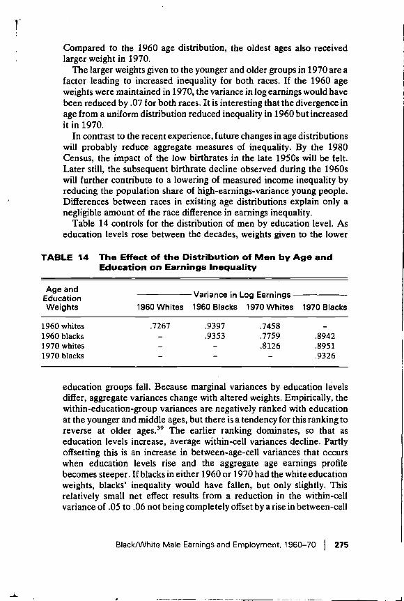
Compared to the 1960 age distribution, the oldest ages also receivedlarger weight in 1970.

The larger weights given to the younger and older groups in 1970 are afactor leading to increased inequality for both races. If the 1960 ageweights were maintained in 1970, the variance in log earnings would havebeen reduced by .07 for both races. It is interesting that the divergence inage from a uniform distribution reduced inequality in 1960 but increasedit in 1970.

In contrast to the recent experience, future changes in age distributionswill probably reduce aggregate measures of inequality. By the 1980Census, the impact of the low birthrates in the late 1950s will be felt.Later still, the subsequent birthrate. decline observed during the 1960swill further contribute to a lowering of measured income inequality byreducing the population share of high-earnings-variance young people.Differences between races in existing age distributions explain only anegligible amount of the race difference in earnings inequality.

Table 14 controls for the distribution of men by education level. Aseducation levels rose between the decades, weights given to the lower

TABLE 14 The Effect of the Distribution of Men by Age andEducation on Earnings Inequality

Age andEducationWeights 1960 Whites

.

Variance in Log Earnings1960 Blacks 1970 Whites 1970 Blacks

1960 whites .7267 .9397 .7458 —

1960 blacks — .9353 .7759 .89421970 whites — — .8126 .89511970 blacks — — — .9326

education groups fell. Because marginal variances by education levelsdiffer, aggregate variances change with altered weights. Empirically, thewithin-education-group variances are negatively ranked with educationat the younger and middle ages, but there is a tendency for this ranking toreverse at older ages.39 The earlier ranking dominates, so that aseducation levels increase, average within-cell variances decline. Partlyoffsetting this is an increase in between-age-cell variances that occurswhen education levels rise and the aggregate age earnings profilebecomes steeper. If blacks in either 1960 or 1970 had the white educationweights, blacks' inequality would have fallen, but only slightly. Thisrelatively small net effect results from a reduction in the within-cellvariance of .05 to .06 not being completely offset by a rise in between-cell


r

Ivariances. Blacks' inequality would have been 4 percent higher in 1970 ifthe 1960 black education weights had been maintained. There was no netchange for whites over time as the reduction in within-cell variance isoffset by higher between-cell variance.

Little is known about the causes of the difference in marginal variancesby education levels. Some of it (especially the high variances for lesseducated males at young ages) is caused by larger employment instability.Variation in schooling quality at different schooling levels and abilityvariation among people completing that level are other explanations.

Because of popular emphasis on between-race differences, there is atendency to neglect the vast disparities that exist within a race. But blacksapparently live in a world in which the pie, albeit a smaller one, isdistributed in a quite uneven manner. In Table A-5 we have listed threeconventional indicators of the economic well-being of blacks andwhites—years of schooling, health status, and quality of schooling. Notsurprisingly, the average levels are lower for blacks. But, the absolute andproportionate variances are hi gher for blacks. Human capital appears to bedistributed more unequally among blacks.

The Census data obviously give a very incomplete explanation for thegreater dispersion in black income. We would like to free ourselves from —

these data constraints and speculate about some of the root causes ofthese differences, but that is a project for another day.

N

S

VII. OCCUPATIONAL AND INDUSTRIALCLASSIFICATIONS

Important changes in occupational and industrial distributions by raceappear to have been in process by 1970. There are always elements ofambiguity in any occupational or industrial classification, so that ourresults can only be viewed as suggestive. Yet, comparisons of this sort L

offer the potential for an insight into the dynamics of race differences in —

economic success that cannot be obtained by reference to earnings alone.Suppose, for example, that the income gains documented in the earliersections had been achieved alongside increasing black-white occupa-tional disparity (segregation) and that blacks were increasingly concen-trated in public sectors of the economy, whereas whites were movingtoward private sectors. In what sense would we be willing to argue that weare moving toward racial parity? Would we be as sanguine about theviability of income gains achieved in this manner as we would in asituation in which black and white income, schooling, occupational, andindustrial distributions were increasingly congruent?

276 Smith and Welch

H

The occupational and industrial classes we use are not standard. Theoccupational classes are deliberately specified to highlight race differ-ences. Subject to a "manageable" number of classes, we combined themore narrowly defined Census groups with an eye to preserving as muchbetween-group wage variance as possible. These combinations were alsodesigned to retain most of the race differences exhibited in narrowerCensus classes in 1960. This procedure permits a simple summary of racedifferences, while preserving the opportunity to observe changes inoccupational congruency between 1960 and 1970.

Table 15 presents 1970 occupational distributions according to tenclasses, separately for blacks who were in the labor market by 1960, for

NOTE: Index of Distributional Congruency(1) x (2) (1)x (3) (2)x (3)

875 .722 .901

black entrants between 1960 and 1969, and for all whites. In recognitionof life-cycle changes in occupational status, the observed distributions forthe first two experience classes have been revised. In examining cohortchanges for whites between 1960 and 1970, there is evidence ofconsiderable occupational change for persons with up to 5 years'experience in 1960.40 There was less dramatic evidence of 1960—70change for those with 6—10 years of experience in 1960, and little change


TABLE 15 Estimatedin 1970(Percent)

Permanent Occupational Distributions

Occupation

Blacks in LaborMarket by 1960

(1)

Blacks Entering1960—69

(2)

AllWhites

(3)

Professors, scientists,artists 2.1 5.2 9.6

Service professionals 1.9 2.1 3.5Managers 2.7 8.4 13.9Skilled clerical and

sales 1.2 5.4 7.3Mechanics, foremen 11.1 12.3 19.4Craftsmen, apprentices 5.0 10.7 5.6Low clerical and sales 8.4 9.0 9.5Operatives 30.9 31.5 19.4Laborers, service

workers 35.3 14.8 10.3Unknown 1.4 0.6 1.5

for those with more than 10 years' work experience. From this, we inferthat although occupational change is often part of the work career, thebulk of this change occurs in the first few years after entering the labormarket. To allow for this career-related change, observed occupationaldistributions for the two cohorts (experience classes 1—5 and 6—10)entering during the sixties are modified according to 1960—70 changes inoccupation observed for the corresponding cohorts a decade earlier. Thisadjustment is given for the jth cohort by

where the index, i, indicates occupation, f* is the adjusted, and f theobserved, proportions of workers in the respective classes.

From Table 15, it is clear that the occupational distribution of blacksentering the labor market in the sixties is sharply different from that ofearlier entrants. We computed an index of congruency to contrast theoccupational distributions in 1970 of blacks who entered the labormarket before 1960 to all whites and to blacks who entered the laborforce between 1960 and 1969. Finally, we compared white to blackentrants during the sixties. The index of congruency between the ith andjth groups is defined as

'ij =

where 1 indexes the occupation and f refers to proportions such that

= =1I I

This index is bounded by 0 (no overlap in distributions) and 1 (completecongruency) and is a first cousin to a simple correlation coefficient. Themain difference is that the denominator is an arithmetic, rather than ageometric, mean.

This index for pre-1960 black entrants and all whites is 0.722. It is0.875 for pre- and post-1960 black entrants and rises to 0.901 for thecomparison of post-1960 blacks to whites. With this measure as ourstandard, the occupational distribution of black entrants during thesixties is more similar to the distribution of whites than it is to otherblacks. We view this as important supplementary evidence of the extentof the gain in relative economic status of blacks realized during the sixties.Table 16 provides black/white indexes of occupational congruency withinschooling and experience classes for 1960 and 1970. It further documentsthe improvement between cohorts exhibited in the earlier wage andearnings comparisons.

278 Smith and Welch

I

TABLE 16 Indexes of Black/White Occupational Congruencyby Schooling and Labor Market Experience, 1960and 1970

Experiencein 1970

—8—11—1970 1960

Years of Schoo

—12——---1970 1960

ling Completed

—13—15—1970 1960

—16+—1970 1960

1—5 .979 — .896 — .874 — .910 —

6—10 .925 — .895 — .816 — .841 —

11—15 .893 .863 .815 .818 .753 .746 .844 .705

16—20 .873 .822 .803 .748 .738 .726 .827 .764

21—25 .871 .819 .774 .755 .735 .714 .832 .850

26—35 .864 .789 .793 .739 .693 .623 .779 .719

Our industrial classes are selected to highlight the potential role ofgovernment in eliminating race differences in wages and employment.Accordingly, there are two categories for direct governmentalemployment—one for the federal government and another for state andlocal governments. An additional two categories refer to aggregates ofindustries regulated by federal and by state and local governments.Finally, there are two classes that we hope measure indirect governmen-tal employment. Assignment to indirect governmental employmentrepresents an attempt to identify the role of governments as consumers ofproducts of private industries. Unfortunately, we do not have dataindicating if an individual works for a firm with government contracts andif this represents an important part of the firm's business. We do,however, have access to data showing government acquisitions byindustry, and we converted these purchases into shares of the respectiveindustry's value added.

When we observe an individual who is not directly employed by agovernment and does not work in a regulated industry, a random numberis drawn from a 0—1 uniform density. If that number is less than thefederal share of the industry's product, the worker is dubbed "indirectfederal employee."4' If the random number lies between the federal andthe aggregate governmental share, the worker is an indirect state andlocal government employee. Otherwise, he "works" in the private(private-private?) sector. This assignment scheme is biased and conser-vative in the sense that black/white changes between 1960 and 1970 areunderstated. In defense, we note only.that we have no clear alternative.We consider it likely that antidiscriminatory legislation is more easilyenforced among firms most dependent on governments for sales. Basedon variation among industries in government revenue shares, we attempt


-J

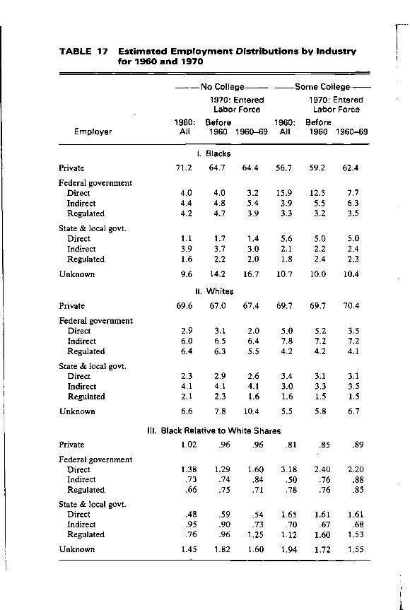
TABLE 17 Estimated Employment Distributions by Industryfor l96Oand 1970

No College —Some College—1970: Entered 1970: Entered

. Labor Force Labor Force

Employer1960:All

Before1960 1960—69

1960:All

Before1960 1960—69

I. Blacks

Private 71.2 64.7 64.4 56.7 59.2 62.4

Federal governmentDirect 4.0 4.0 3.2 15.9 12.5 7.7Indirect 4.4 4.8 5.4 3.9 5.5 6.3Regulated 4.2 4.7 3.9 3.3 3.2 3.5

State & local govt.Direct 1.1 1.7 1.4 5.6 5.0 5.0Indirect 3.9 3.7 3.0 2.1 2.2 2.4Regulated 1.6 2.2 2.0 1.8 2.4 2.3

Unknown 9.6 14.2 16.7 10.7 10.0 10.4

II. Whites

Private 69.6 67.0 67.4 69.7 69.7 70.4

Federal governmentDirect 2.9 3.1 2.0 5.0 5.2 3.5Indirect 6.0 6.5 6.4 7.8 7.2 7.2Regulated 6.4 6.3 5.5 4.2 4.2 4.1

State & local govt.Direct 2.3 2.9 2.6 3.4 3.1 3.1Indirect 4.1 4.1 4.1 3.0 3.3 3.5Regulated 2.1 2.3 1.6 1.6 1.5 1.5

Unknown 6.6 7.8 10.4 5.5 5.8 6.7

Ill. Black Relative to White Shares

Private 1.02 .96 .96 .81 .85 .89

Federal governmentDirect 1.38 1.29 1.60 3.18 2.40 2.20Indirect .73 .74 .84 .50 .76 .88Regulated .66 .75 .71 .78 .76 .85

State & local govt.Direct .48 .59 .54 1.65 1.61 1.61Indirect .95 .90 .73 .70 .67 .68Regulated .76 .96 1.25 1.12 1.60 1.53

Unknown 1.45 1.82 1.60 1.94 1.72 1.55

to estimate age and schooling distributions by race among employees offirms whose product is produced for governments, in contrast to age-schooling employment distributions among firms whose product is pro-duced for use in the private sector.

Table 17 summarizes our information of changes in industrial distribu-tions. Employment shares by industrial group are given for blacks (panelI), whites (panel II) and for blacks relative to whites (panel III) as of1960, and in 1970 for pre- and post-1960 entrants separately for thosewho had no more than twelve years of schooling and for the combined13—15 and 16+ classes. The most notable change occurred for those whohad some college education. The relative black share dropped sharplybetween 1960 and 1970 in direct federal employment (where 16 percentof all blacks who had attended college were employed in 1960, incomparison to 5 percent of whites). The most pronounced increase inemployment shares of blacks who had attended college between 1960and 1970 was in the private-private and the indirect federal sectors. Thedrop in direct federal employment shares for blacks accompanied a(somewhat less pronounced) drop for whites and suggests that at least forthose who have attended college, the federal government is less of a"growth industry" than many would imagine. The increase in the privatesector employment of blacks who have attended college would seem to bereason for optimism, although the more-than-proportionate increase inthat part of the private sector whose product is purchased by the federalgovernment suggests that this change may have been associated, in part,with some "arm twisting."

VIII. CONCLUSION

There are many ways of slicing up data, but whatever one's angle ofvision, the improvement in the relative income of black males during the1960s is impressive. Equally eye-catching is the universal sharing of thesegains across experience and schooling classes. Those whose relativeposition improved most are more likely to be the most educated and themore recent entrants into the labor market.

We feel the data summarized offer a mildly optimistic picture for blackrelative wages. First, the most pronounced gains in earnings ratios areassociated with increased schooling levels, and black school completioncontinues to rise relative to white levels. Second, younger cohorts farebetter than their older peers. Whatever the cause of the inter-cohortdifferentials exhibited in 1970, if the experience of the sixties is a basis forprediction, wage ratios within cohorts will not decline as time passes, atleast, not by very much.


Viewed from the historical perspective of relatively constant ordeteriorating black/white wages, the experience of the sixties isencouraging. It is still important to note that although the patterns ofgains found between 1960 and 1970 suggest that earnings will rise forblacks relative to whites, the rate of increase is likely to be slow. Amongthose who were in the work force in both years, 1960 and 1970, blackrelative earnings increased from 0.57 to 0.62. The aggregate ratio in 1970is roughly 0.64 when the higher earnings of new entrants are taken intoaccount.

If the most optimistic view is taken and the relative wage of new blackentrants changes by the same amount (11.8 percent) in each new decadeas it did between 1960 and 1970, and if the within-cohort growthcontinues at 0.04, we shall have to wait until the Census of 2000 beforeparity for new entrants is achieved. Full racial parity would take another40 years, so that few of us will be alive to see it. Since the improvement inthe 1960s was exaggerated by the business-cycle gains, racial incomeequality will probably take a good deal longer and could easily be partlynullified by a two or three percentage point increase in the unemploymentrate.

Many have argued that the rise in black/white wage ratios over thesixties is the effect of enforced compliance to fair employment legislationof what is popularly known as affirmative action. While this issue is notaddressed directly, we have compiled some indirect evidence that theeconomic impact of this legislation is probably overrated. Based on ourwork, the largest gains in black/white wage ratios have occurred inindustries least vulnerable to federal or local government "arm twisting."

APPENDIXTABLE A-i Proportion with Zero Earnings

Years ofExperience

Ed

8

White 1960:ucation Gro

12 16

up

AU

Ed

8

Black 1960:ucation Gro

12 16

up

All

1—5 .179 .030 .021 .058 .273 .101 .046 .1866—10 .083 .013 .007 .029 .120 .066 .009 .109

11—15 .022 .015 .005 .025 .099 .065 .039 .08416—20 .033 .099 .008 .027 .109 .052 — .08821—30 .038 .018 .015 .032 .097 .069' .036 .08731—40 .053 .051 .105 .059 .112 .087 .105 .111

282 Smith and Welch

4.

TA

BLE

A-2

Reg

ress

ion

Res

ults

for

Com

bine

d S

ampl

es o

f Bla

ck a

nd W

hite

Mal

es in

196

0 an

d 19

70, b

yY

ears

of W

ork

Exp

erie

nce'

Exp

erie

nce

Cla

ss

—1

to5

Yea

rs—

—6

to10

Yea

rs—

—11

to15

Yea

rs—

—16

to20

Yea

rs—

—21

1030

Yea

rs—

—31

to40

Yea

rs—

Ful

lC

on-

Ful

lC

on-

Ful

lC

on-

Ful

lC

on-

Ful

lC

on-

Ful

lC

on-

Inte

r-st

rain

edIn

ter-

stra

ined

Inte

r-st

rain

edIn

ter-

stra

ined

Inte

r-st

rain

edin

ter-

stra

ined

Inte

ract

ion

actio

nE

stim

ates

actio

nE

stim

ates

actio

nE

stim

ates

actio

nE

stim

ates

actio

nE

stim

ates

actio

nE

stim

ates

I. S

choo

ling

A.

Gra

de sc

hool

.137

6.1

434

.107

5.1

006

.066

6.0

687

.061

4.0

623

.057

8.0

585

.046

6.0

495

(18.

86)

(27.

56)

(21.

38)

(28.

34)

(14.

58)

(22.

69)

(13.

91)

(22.

10)

(19.

89)

(29.

35)

(15.

26)

(22.

45)

Rac

e—

.045

7—.0460

—.0148

—.0176

—.0134

—.0151

—.0164

—.0187

—.0279

—.0269

—.0188

—.0234

(4.79)

(6.91)

(2.29)

(3.96)

(2.28)

(3.9

6)(2.84)

(5.24)

(7.2

9)(10.65)

(4.6

5)(8

.28)

Year

.011

5—

—.0

119

—.0

044

—.0

021

—.0

013

—.0

066

—

(1.1

0)—

(1.6

5)—

/(.

71)

—(.

36)

—(.

32)

—(1

.46)

—

Rac

e-ye

ar—

.004

5—

—.0

113

——

.004

5—

—.0

042

—.0

007

——

.011

5—

(.34

)—

(1.2

3)—

(.56

)—

(.55

)—

(.13

)—

(1.9

5)—

B.

Col

lege

.122

5.1

237

.088

0.0

927

.090

1.0

920

.088

2.0

881

.075

7.0

773

.074

4.0

744

(24.

98)

(28.

87)

(20.

86)

(26.

01)

(21.

88)

(26,

96)

(19.

58)

(23.

81)

(20.

23)

(24.

39)

(13.

27)

(15.

25)

Rac

e.0

390

.033

6.0

117

—.0

070

——

.000

7—

.008

9—

.000

6—

(3.8

4)(4

.25)

(1.4

2)—

(.89

)—

(.09

)—

(1.1

7)—

(.05

)—

Yea

r—.0241

—.0243

—.0078

—.0107

—.0108

—.0135

—.0200

—.0233

—.0038

—.0076

—.0254

—.0244

(3.13)

(3.7

5)(1

.18)

(1.9

9)(1

.64)

(2.5

6)(2

.79)

(3.9

7)(.6

4)(1

.51)

(2.5

9)(2

.94)

Rac

e-ye

ar—

.005

5—

—.0

079

——

.011

2—

—.0

126

——

.021

0—

—.0

018

—

(.34

)—

(.62

)—

(.89

)—

(.91

)—

(1.6

9)—

(.08

)—

ii. L

ocat

ion

A.

Nor

th C

entra

l—

.022

3—

.021

2—

.006

8.0

307

.015

0.0

366

.037

6.0

510

.035

0.0

474

(.82)

—(.

93)

—(.

31)

(2.5

6)(.6

6)(3

.23)

(2.2

7)(5

.90)

(1.8

2)(4

.57)

Rac

e—

.106

4.0744

.1299

.1410

.0360

—.0

056

—.0

060

—.0

127

—

(2.5

0)(2

.44)

(3.6

9)(5

.56)

(1.0

5)—

(.16

)—

(.23

)—

(.41

)—

Yea

r.0

412

——

.001

8—

.037

0—

.017

4—

.034

3—

—.0

115

—

(1.0

1)—

(.05

)—

(1.1

8)—

(.56

)—

(1.4

6)—

(.41

)—

F

TA

BLE

A-2

(con

tinue

d)

—1

to5

Yea

rs—

—6

to10

Yea

rs—

—11

to

Exp

erie

nc

15 Y

ears

—

e C

lass

—16

to20

Yea

rs—

—21

to30

Yea

rs—

—31

to40

Yea

rs—

Ful

lIn

ter-

Inte

ract

ion

actio

n

Con

-st

rain

edE

stim

ates

Ful

lIn

ter-

actio

n

Con

-st

rain

edE

stim

ates

Ful

lIn

ter-

actio

n

Con

-st

rain

edE

stim

ates

Ful

lIn

ter-

actio

n

Con

-st

rain

edE

stim

ates

Ful

lIn

ter-

actio

n

Con

-st

rain

edE

stim

ates

Ful

lIn

ter-

actio

n

Con

-st

rain

edE

stim

ates

Il. L

ocat

ion

(con

tinue

d)

Rac

e-ye

ar—

.130

8—.0821

—.1281

—.1234

—.0530

—.0

446

——

.029

1—

.055

1

(1.9

6)(1

.66)

(2.4

4)(3

.20)

(1.0

8)—

(.92

)—

(.78

)—

(1.2

2)

B.

Sou

th—

.145

4—

.132

3—

.122

6—

.129

0—

.092

1—

.083

7—

.125

7—

.082

6—

.073

3—

.091

5—

.108

9—

.102

6(5

.31)

(7.7

1)(5

.27)

(8.8

8)(4

.08)

(5.4

8)(5

.33)

(5.5

9)(4

.29)

(8.2

4)(5

.42)

(7.6

3)Race

—.0

178

—.0

169

—.0

897

—.0

970

—.1

553

—.1

580

—.1

768

—.2

008

—.2

249

—.2

110

—.1

777

—.1

985

(.44)

(.54)

(2.65)

(3.7

0)(4

.77)

(6.8

6)(5

.20)

(10.16)

(8.9

4)(1

4.04

)(5

.89)

(11.00)

Yea

r.0

170

.006

3—

.012

1—

.068

5—

—.0

345

——

.002

0—

(.41

)—

(.18

)—

(.37

)—

(2.0

8)—

(1.3

9)—

(.07

)—

Rac

e-ye

ar—

.128

9—

.152

1—

.060

2—

.045

3—

.036

5—

.044

0—

.009

6—

.017

1—

—.0

226

—

(2.0

2)(3

.62)

(1.1

7)(1

.37)

(.77)

(1.6

9)(.2

0)—

(.47

)—

(.51

)—

C.

Wes

t—

.069

3—

.044

1—

.067

7—

.065

1—

.056

8—

.036

9—

.018

6—

.011

7—

—.0

082

—

(2.3

2)(2

.01)

(2.6

1)(3

.46)

(2.3

0)(1

.95)

(.72)

—(.

61)

—(.

36)

—

Rac

e.0

454

—.0

406

—.0

369

—.0

066

——

.030

7—

—.0

374

—

(.86

)—

(.92

)—

(.85

)—

(.15

)—

(.90

)—

(.89

)—

Yea

r.0

802

.042

3.0

896

.078

0.1

359

—.0

988

.027

8.0

138

.029

3.0

461

.055

2.0

516

(1.7

1)(1

.23)

(2.3

3)(2

.77)

(3.7

5)(3.77)

(.77)

(.72)

(1.0

5)(2

.96)

(1.6

3)(2

.67)

Rac

e-ye

ar—

.061

9—

—.0

229

——

.087

5—

.044

4—

.052

1—

.050

0—

(.72

)—

(.34

)—

(1.3

5)—

(.70

)—

(1.0

4)—

—

D.

Met

ropo

litan

.035

7.0

192

.109

2.0

966

.169

8.1

387

.172

8.1

467

.185

0.1

693

.218

5.1

905

(1.6

0)(.9

6)(5

.80)

(5.7

6)(9

.21)

(8.5

2)(8

.96)

(8.8

7)(1

3.09

)(1

3.79

)(1

3.07

)(1

3.11

)R

ace

—.0

211

.001

3—

.047

7—

.016

1—

.117

5—

.044

9—

.073

5—

.031

3—

.095

0—

.070

2—

.075

0—

.038

5(.5

6)(.0

4)(1

.44)

(.65)

(3.6

9)(1

.95)

(2.1

9)(1

.35)

(3.9

0)(4

.00)

(2.6

4)(1

.86)

Yea

r.1

293

.166

3.0

524

.075

5—

.006

0.0

566

.026

3.0

823

.036

7.0

669

.041

0.1

048

(3.7

1)(6

.79)

(1.8

3)(3

.72)

(.22)

(2.9

6)(.9

6)(4

.44)

(1.7

6)(4

.81)

(1.6

2)(6

.43)

Rac

e

Yea

r

Rac

e-ye

ar

H

Rac

e-ye

ar.0

330

(.54)

— —

.066

3(1

.33)

— —

.1473

—.0

861

(3.1

9)—

(1.8

5)— —

0489

(1.3

9)— —

.084

3(2

.02)

E.C

entra

l city

—.0

379

(1.6

5).0

517

(1.4

6)—

.039

0(1

.08)

.170

5(2

.96)

—.0

555

(3.1

4).1

138

(4.0

9)— — — —

—.0

765

(3.7

9).0

976

(3.18)

.016

0(.5

3).0

094

(.20)

—.0

686

(4.5

9).0

982

(4.25)

— — — —

—.0

922

—.0

942

—.0

999

(4.5

7)(6

.50)

(4.8

1).1

518

.1629

.1042

(5.07)

(7.5

0)(3

.37)

—.0

012

—.0

160

(.04)

—(.

55)

.019

1—

.073

1(.4

4)—

(1.6

9)

—.0

946

(6.5

8).1

437

(6.66)

— — — —

—.0

460

(3.0

7).1

204

(5.31)

—.0

253

(1.1

6).0

411

(1.2

4)

—.0

576

(5.3

1).1

382

(8.38)

— — — —

—.0

554

(3.2

0).1376

(5.15)

.018

3(.7

0).0102

(.26)

F.Y

ears

in c

urre

ntre

side

nce

Rac

e

Yea

r

Rac

e-ye

ar

—.0

158

(9.4

8).0

064

(2.7

2).0

04 1

(1.6

1)—

.001

0(.2

8)

—.0

112

(12.

54)

— — — — — —

—.0

072

(4.4

0)—

.003

4(1

.52)

.000

0(.0

1).0

034

(1.01)

—.0

083

(9.9

9)— — — — — —

—.0

037

—.0

039

—.0

003

(2.3

5)(5

.03)

(.19)

—.0

005

——

.000

1(.2

2)—

(.08

)—

.000

4—

—.0

006

(.20)

—(.

32)

.001

1—

.001

8(.3

7)—

(.64

)

— — — — — — — —

.000

2(.2

0)—

.001

0(.8

2).0

005

(.37)

.0033

(1.8

5)

— — — — — — — —

—.0

006

(.67)

.002

7(2

.21)

.003

6(2

.91)

—.0

020

(1.09)

III.

Gov

ernm

ent E

mpl

oym

ent

A.

Fede

ral e

mpl

oyee

Rac

e

Yea

r

Rac

e-ye

ar

.103

7(1

.59)

.0234

(.28)

—.1035

(1.0

7).2

034

(1.6

3)

.052

2(1

.09)

.0663

(.93)

— —

.112

0(1

.43)

.086

5(1

.77)

.0717

(1.08)

—.0124

(.18)

.102

0(1

.08)

.075

6(2

.14)

.105

4(1.86)

— —

.055

9(.9

0)

.073

7.0

829

.052

8(1

.65)

(2.6

4)(1

.20)

.095

7.0950

.1648

(1.58)

(1.86)

(2.83)

.0235

—.0

180

(.37)

—(.

31)

.079

5.0

920

.043

3(.9

4)(1

.68)

(.55)

.061

2(2

.11)

.148

9(3.15)

— —

.081

8(1

.60)

.083

8(3

.04)

.156

1(4.01)

—.0392

(.94)

.119

2(2

.04)

.066

6(3

.24)

.168

1(4.96)

— —

.092

9(2

.31)

.159

6(4

.53)

.118

8(2.39)

—.0115

(.20)

.067

6(.8

5)

B.

Industry regulated

by

fede

ralg

ovt.b

Rac

e

Yea

r

Rac

e-ye

ar

.1534

(3.34)

.061

9(.8

8)—

.027

7(.3

8).0

350

(.28)

.1694

(6.09)

— — — — — —

.1218

(3.46)

—.0

238

(.42)

.0135

(.25)

.1476

(1.6

5)

.1394

(6.63)

— — — — — —

.0949

.0870

.1364

(2.82)

(4.6

6)(3

.95)

—.0

209

——

.079

0(.40)

—(1

.44)

—.0

162

—.0

202

(.34)

—(.

43)

.046

0—

.016

6(.59)

—(.

22)

.1191

(6.54)

— — — — — —

.1211

(4.93)

—.0

455

(1.1

3).0

044

(.12)

.0441

(.79)

.1148

(8.45)

— — — — — —

.1631

(5.37)

—.1

329

(2.9

0)—

.019

8(.4

6).2

157

(3.3

5)

—.0478

(3.70)

.1411

(7.1

8)

.1584

(5.7

6).1

2 11

(2.7

5)

.0581

(1.0

7).1

447

(9.0

6)

TA

BLE

A-2

(con

clud

ed)

—ito

5 Y

ears

——

6 to

10 Y

ears

——

11 to

Exp

erie

nc

15 Y

ears

—

e C

lass

—16

to20

Yea

rs—

—21

to30

Yea

rs—

—31

to40

Yea

rs—

Ful

lIn

ter-

Inte

ract

ion

actio

n

Con

-st

rain

edE

stim

ates

Ful

lIn

ter-

actio

n

Con

-st

rain

edE

stim

ates

Ful

lIn

ter-

actio

n

Con

-st

rain

edE

stim

ates

Ful

lIn

ter-

actio

n

Con

-st

rain

edE

stim

ates

Ful

lIn

ter-

actio

n

Con

-st

rain

edE

stim

ates

Ful

lIn

ter-

actio

n

Con

-st

rain

edE

stim

ates

Ill. G

over

nmen

t Em

ploy

men

t (co

nclu

ded)

4C

.Fe

dera

l sha

re o

f.3

629

.407

3.2

050

.2997

.2712

.3177

.1976

.2560

.2356

.2833

.2501

.3212

industry

prod

uctc

(4.9

7)(7

.17)

(3.1

4)(6

.53)

(4.2

9)(7

.29)

(3.0

6)(5

.88)

(5.0

3)(8

.33)

(4.5

4)(7

.53)

Race

.242

4.1

754

.096

2.0042

.1410

.0622

.2222

.1658

.2284

.1619

.5248

.4282

(2.10)

(1.6

7)(.9

4)(.05)

(1.3

4)(.6

7)(2

.11)

(1.7

9)(2

.68)

(2.1

0)(5

.05)

(4.48)

Year

.102

9—

.183

6—

.082

9—

.111

1—

.101

4—

.186

2—

(.88

)—

(1.9

9)—

(.95

)—

(1.2

7)—

(1.4

9)—

(2.1

3)—

Rac

e-ye

ar.4

814

.654

9.2343

.401

2.1

863

.320

2.3

757

.4916

.386

6.5

269

.244

6.5

261

(2.1

8)(3

.63)

(1.3

6)(2

.85)

(1.22)

(2.6

4)(2

.48)

(4.0

8)(3

.06)

(5.1

2)(1

.53)

(4.10)

D.

Stat

e an

d lo

cal g

ovt.

.597

3.5

188

.593

8.4

2 10

.544

0.4

423

.403

0.3

760

.500

4.3

938

.387

4.3

583

shar

e of

indu

stry

(4.5

2)(6

.87)

(5.5

2)(7

.08)

(5.5

2)(8

.22)

(3.9

9)(7

.19)

(6.3

8)(9

.80)

(4.2

2)(7

.54)

prod

uctc

Rac

e—

.227

5—

—.3

636

——

.371

7—

.066

0—

—.0

867

—.0

351

(1,0

9)—

(2.1

8)—

(2.4

2)—

(.43

)—

(.76

)—

(.26

)Year

—.2227

——

.179

2—

—.1

039

——

.038

7—

.212

9—

—.0

856

(1.14)

—(1

.13)

—(.

71)

—(.

27)

—(1

.90)

—(.

65)

Race-year

.602

4—

.339

8—

.491

8—

—.1

323

—.1

675

—.0

004

(1.94)

—(1

.41)

—(2

.26)

—(.

63)

—(1

.04)

—(.

00)

IV.

Exp

erie

nce

A.

Years

.2361

.1871

.2111

.1020

.0522

.0593

—.0348

.110

4—.0713

—.0140

.0585

—.0344

(6.69)

(9.43)

(2.66)

(2.40)

(.42)

(.91)

(.19)

(1.2

2)(1

.64)

(.62)

(.82)

(.92)

Rac

e—

.039

0—

—.1

465

——

.220

2—

.129

0—

.047

9—

—.1

553

—

(.75

)—

(1.2

7)—

(1.2

0)—

(.49

)—

(.75

)—

(1.4

9)—

Yea

r—

.036

6—

—.1

357

—.0

975

—.0

082

—.0

953

——

.08

17—

(.68

)—

(1.1

6)—

(.54

)—

(.03

)—

(1.5

3)—

(.82

)—

'S

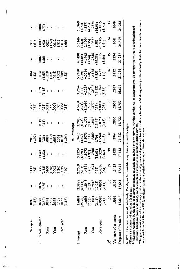
c

Race-year

—.0916

—.1

117

—.2

813

—.3

172

——

.048

4—

.091

1(1.13)

—(.

65)

—(1

.07)

—(.

87)

—(.

53)

—(.

61)

B.

Years

squa

red

—.0

220

—.0156

—.0115

—.0040

—.0012

—.0015

.0013

—.0029

.0014

.0002

—.0009

.0004

(3.80)

(4.86)

(2.32)

(1.52)

(.26)

(.61)

(.25)

(1.15)

(1.65)

(.56)

(.92)

(.77)

Race

.0048

—.0

100

—.0

084

——

.003

8—

—.0

010

—.0

022

—

(.56

)—

(1.3

8)—

(1.1

9)—

(.53

)—

(.82

)—

(1.5

2)—

Yea

r.0035

—.0

092

——

.003

8—

—.0

004

——

.001

8—

.001

2—

(.40

)—

(1.2

6)—

(.56

)—

(.06

)—

(1.5

2)—

(.81

)—

Rac

e-ye

ar.0152

——

.007

5—

—.0

105

——

.008

6—

.000

9—

—.0

014

—

(1.1

6)—

(.70

)—

(1.0

4)—

(.85

)—

(.52

)—

(.66

)—

V. I

nter

cept

Inte

rcep

t2.6091

2.5998

2.7609

3.2324

3.7615

3.7070

4.5404

3.2696

5.2380

4.5490

3.5146

5.0960

(25.20)

(40.13)

(8.07)

(18.91)

(4.47)

(8.76)

(2.9

1)(4

.01)

(9.2

9)(1

5.85

)(7

.70)

Rac

e.2

661

.2043

.4171

—.1072

1.3076

—.1571

—1.1697

—.1227

—.5516

—.0463

2.4904

—.1371

(2.03)

(2.5

9)(.91)

(1.97)

(1.11)

(3.40)

(.50)

(2.84)

(.68)

(1.54)

(1.36)

(4.23)

Year

—.3

411

—.2

818

.347

4—

.260

0—.8809

—.2418

—.2770

—.2308

—1.4538

—.2535

1.0677

—.2

574

(2.4

1)(1

2.08

)(.7

5)(13.65)

(.76)

(13.45)

(.12)

(13.12)

(1.85)

(19.28)

(.58)

(16.66)

Race-year

—.0

393

—.0

962

—.4

336

—.0

620

—1.

9944

—.0

754

—3.

0981

—.1

078

.473

7—

.081

5—1.5005

—.1015

(.21)

(2.4

7)(.6

4)(2

.02)

(1.1

8)(3

.16)

(.95)

(5.5

2)(.4

1)(5

.44)

(.57)

(5.73)

R2

.36

.36

.39

.39

.39

.39

.38

.38

.36

.35

.34

.33

Var

ianc

e of

est

imat

e.5

096

.5 1

03.3

423

.342

8.2

964

.296

5.2

955

.295

7.3

232

.323

4.3

641

.364

9D

egre

esof

free

dom

17,6

1317

,641

17,4

1317

,442

16,7

2216

,722

16,7

5216

,609

31,2

5431

,287

24,8

9924

,932

NO

TE: O

bser

vatio

ns a

re o

f ind

ivid

uals

. The

dep

ende

nt v

aria

ble

is lo

g, b

ase

e,of

wee

kly

wag

es.

ames

e ar

e es

timat

es o

f equ

atio

n 1

inth

e te

xt.

blnd

ustn

esre

gula

ted

by th

efe

dera

l gov

ernm

ent i

nclu

de ra

ilroa

ds a

nd ra

ilway

exp

ress

serv

ice,

truc

king

serv

ice,

wat

er tr

ansp

orta

tion,

air

trans

porta

tion,

radi

o br

oadc

astin

g an

dte

levi

sion

, tel

epho

ne (w

ire a

nd ra

dio)

, and

tele

grap

h an

d m

isce

llane

ous c

omm

unic

atio

n se

rvic

es.

cThe

gove

rnm

ent

shar

e of

the

indu

stry

pro

duct

is th

e ra

tio o

f gov

ernm

ent p

urch

ases

from

the

indu

stry

to v

alue

add

ed o

rigin

atin

g in

the

indu

stry

. Dat

a fo

r the

sew

ere

obta

ined

from

BLS

Bul

letin

197

2;re

sulta

ntsh

ares

are

ava

ilabl

e on

requ

est f

rom

the

auth

ors.

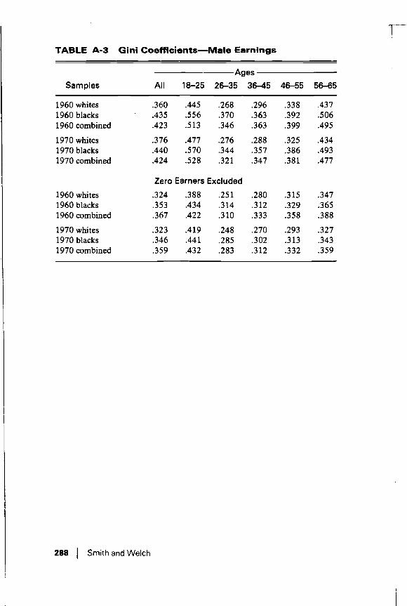
TABLE A-3 Gini Coefficients—Male Earnings T

Ages

Samples All 18—25 26—35 36—45 46—55 56—65

1960 whites .360 .445 .268 .296 .338 .4371960 blacks .435 .556 .370 .363 .392 .5061960 combined .423 .513 .346 .363 .399 .495


Zero Earners Excluded



SdLaGc

SdLaGa

W4

Sd

LaGa

W

SdLaGa

WI

Go

WI

SdLqGa

288 Smith and Welch W

L

TABLE A-4 Explained Variance Summary(o2 = variance in annual earnings; oj = explainedvariance in annual earnings; oj = explained variance inweekly wages)

Whites 1970— —Whites 1960(1) (2) (3) (4) (1) (2) (3) (4)

I. Experience Class, 1—5 Years

a-2— 2857;23932 110

Schooling (1) .040 .004 .003 .035 .054 .010 .003 .064Location (2) .008 .000 .007 .016 .001 .016Government

employment (3) .006 .002 .006 .004Weeksworked(4) .138 .187

Schooling (1)Location (2)Government

employment (3)Weeks worked (4)

Ill. Experience Class, 11—l5Years2370;2070:2031 2397.2 126.2044

.016 .002 .001 .005 .022 .005 .001 .013.007 .000 .001 .012 .001 .002

.004 —.000 .004 —.001.067

IV. Experience Class, 16—20 Years

2419o2077cr2030 a-2— 389o-2= 125a-2 044

Schooling(1) .016 .003 .000 .007 .021 .006 .000 .011Location (2) .008 .000 .002 .013 .001 .003Government

employment (3) .003 —.001 .003 —.000Weeks worked (4) .066

V. Experience Class, 2 1—30 Years

034.017 .003 .000 .006 .020 .007 —.000 .013

.010 .000 .002 .016 .000 .004

.003 —.001 .003 —.001.043

VI. Experience Class, 31—40 Yearsa-2— 535.2 1772 053

.016 .004 .001 .005 .016 .007 —.000 .012

.012 .000 .003 .024 .001 .007

.010 .002 .018 —.001

.105

II. Experience Class, 6—10 Years

2481;2_129;2 .048 2533;2193;2063.030 .003 .001 .018 .036 .006 .002 .029

.007 .000 .002 .012 .001 .005

.004 .000

.058

Schooling (1)Location (�)Government


.004 .001

.093

.034

.039





.085

.064

TABLE A-4 (concluded)

Blacks 1970 Blacks 1960

(1) (2) (3) (4) (1) (2) (3) (4)

I. Experience Class, 1—5Years

21130;24:30;2 090 21187;2591;2206Schooling (1) .030 .008 .003 .041 .056 .041 .009 .037Location (2) .020 .001 .012 .060 .009 .005Government

employment (3) .008 .005 .015 .001Weeks worked (4) .268 .327

II. Experience Class, 6—10 YearsC

.730; .256; .094 u2— .819; .150

Schooling (1) .036 .014 .003 .021 .051 .036 .007 .023Location (2) .034 —.000 .003 .043 .005 .013Government —

employment (3) .004 .001 .008 .001Weeks worked (4) .135 .207 C

Ill. Experience Class, YearsC

g2— .551; .14.8; .064 .695; .117

Schooling(1) .0(8 .010 .002 .006 .025 .023 .005 .011Location (2) .028 .000 .002 .048 .005 .002Government

employment (3) .004 —.000 .010 .002Weeks worked (4) .077 .181

IV. Experience Class, 16—20 Years

a-2— .536; .149; .069 o2= .608; .273; .116

Schooling(1) .013 .011 .002 .004 .019 .022 .004 .010Location (2) .036 .001 .003 .051 .007 .005Government

employment (3) .006 —.000 .013 .002Weeks worked (4) .074 .140

V. Experience Class, 21—30 Years

2555. 2.- 648

Schooling (1) .009 .012 .002 .003 .011 .017 .003 .008Location (2) .043 .002 .003 .057 .007 .001 C

Governmentemployment (3) .006 .001 .014 .001

Weeks worked (4) .083 .168

VI. Experience Class, 31—40 Years

Schooling (1) .007 .012 .002 .004 .007 .016 .002 .006Location(2) .053 .003 .005 .077 .011 .009Government

employment (3) .010 .002 .018 —.001Weeks worked (4) .093 .176

NOTE: In the first experience class, experience accounts for 2.9 so 6.5 percent of explained variance, and thecovariance between experience and weeks worked accounts for 2.5 to 3.8 percent. In other classes, experiencewithin intervals accounted for little wage variation.

TABLE A-5 Measures of Variation in Alternative Indicators ofWell-Being

Measure

Schooling8

Experience Group

1—5 6—10 11—15 16—20 21—30 31—40

Variance 1960 blacks 7.056 10.86 11.7 12.50 13.62 12.7Variance 1960 whites 7.475 9.29 9.71 9.67 10.19 10.0Coefficient of variation

1960 blacks .2070 .2774 .3052 .3322 .3937 .440Coefficient of variation

1960 whites .1889 .2180 .2326 .2399 .2585 .285

Health Statusb

Blacks WhitesMeasure

c.v. Proportion in good health .7895 .7106c.v. Length of latest health

limitation .823 1 .6098

Selected 12-Grade School Characteristicsc

Blacks —Whites---—-—Characteristic Mean S.D. Mean S.D.

Teachers' experience 11.66 3.21 10.72 3.10Quality of teachers' college 6.74 .103 .741 .046Teachers' verbal ability 21.2 2.56 23.1 1.48Teachers' salary (dollars) 6464.8 1494 6745.6 1210Pupil/teacher ratio 25.8 12.1 23.1 8.65Days in session 179.9 4.14 179.4 4.03Attendance (percent) 91.4 3.67 94.3 2.38Library volumes per student 4.65 3.99 5.65 4.01

aus Census.b1966 Surveyof Economic Opportunity data. For derivation, see James P. Smith, "Life Cycle Allocation of Timein a Family Context," Ph.D. dissertation, University of Chicago, 1972.

Ciames S. Coleman et al., Equality of Educational Opportunity, OE 38001, U.S. Office of Education, 1966.

he


NOTES1. This paper is in part a compilation of two earlier papers: "Black/White Wage Ratios:

1960—1970" and "Inequality: Race Differences in the Distribution of Earnings." Itcontains a good deal of additional supporting evidence and a shorter version wasissued as a final report to the Department of Labor by the Rand Corporation. (SeeR-1666, June 1975.)

2. See his Economics of Discrimination, page 140. Becker simply used income byoccupation data in 1940 to weight the occupations. Therefore, a secular increase in hisindex would imply that blacks were moving more rapidly than whites into occupationsthat had high wages in 1940.

3. See James Gwartney [5].4. Before 1965, the Current Population Survey (CPS) did not provide a black/white

income ratio. Because other nonwhites have higher incomes than blacks do, thenonwhite to white income ratio exceeds the ratio of black to white incomes.Fortunately, for an analysis of secular trends the two ratios appear to move together.Therefore, the ratio of nonwhite to white income provides an accurate picture of thelong-term trends in black/white income ratios.

5. As assumed from Table 3:

SCHOOL LEAVING AGE

Schooling level (years) 0—7 8 9—11 12 13—15 16 17 and aboveAge 14 16 18 20 23 25 28

6. Weekly wages are earnings last year divided by weeks worked last year. The averageweekly wage used here is total earnings of all persons divided by total weeks worked,i.e., individual earnings per week are weighted by weeks worked.

7. The sole exception is for weekly wages of elementary school graduates for the cohortwith 31 to 40 years of work experience in 1970.

8. We have also excluded males with zero earnings from this study. Table A-i of theAppendix describes the left-out group.

9. In particular, the recently available 1-in-100 Public Use Samples contain state ofresidence identification, so that these data on wages and weeks worked can be mergedwith other sources which indicate state-specific levels of economic activity.

10. Available evidence of the distribution of cyclic effects refers to employment ratherthan wages (see Kosters and Welch [8] and Kalachek [7]). Yet it is hard to conceive ofa "theory" of wage flexibility that predicts negative correlation between employmentand wage changes.

11. A number of "secondary labor market" hypotheses have been put forward to describeearnings and job progress over working careers. The presumption underlying thesetheories is that some jobs, those dubbed "secondary," are dead-end, with littleprospect for career progress in wages and job status, while other jobs facilitate upwardmobility. Persons who seem likely candidates for secondary careers are disproportion-ately black and less schooled. The observed relative wage performance of blacksduring the sixties is not consistent with these theories.

12. A life-cycle argument has been suggested in Jacob Mincer's work [9]. The observedconvergence in relative wages by skill level could be rationalized in Mincer's humancapital model by a negative correlation between initial postschool earning capacityand the proportion of time spent in job-related investment activities.

13. One interesting possibility is that job markets are less discriminatory than schools, sothat, relative to whites, blacks have a comparative advantage in acquiring skills on thejob rather than in school.

292 Smith and Welch

. . .

14. Degrees of freedom in each of the regressions are large, so that the normal approxima-tion can be used. In the 24 regressions (6 experience classes, 2 races, and 2 years) theabsolute value of the computed f-statistic exceeds 1.96 in 19 of 24 cases, with thelargest calculated value being 7.2 for blacks in 1970 with 2 1—30 years of experience.Exceptions include: (1) blacks 1970, 6—10 years of experience (1:1 = 0.6); (2) whites1960, 6—10 years (JtJ = 1.8); (3) whites 1960, 16—20 years (Jtj = 1.5); (4) whites 1960,31—40 years (Iti = 0.4); and (5) blacks 1960, 31—40 years (fri = 1.4).

15. In preliminary analysis a variable was also included to indicate whether an individualwas an employee of state and local government, and this variable was permitted tointeract with the one denoting Southern residence. Nb consistent pattern emerged,and the variable for employment by state and local governments was deleted insubsequent estimates.

16. If Q1 is the sum of squared residuals for the ith group and df1 is the associated degreesof freedom, then the estimate of residual variance within group is = Q./df1 and forthe pooled sample it is S2 =

17. The potential loss is the bias entailed by incorrect constraints.18. Of the 186 coefficients deleted in constrained estimation, 12 have associated

f-statistics exceeding 2.0 (in absolute value) computed from the fully interactiveequations.

19. The computed F-statistics are:

Experience class= 1—5 6—10 11—15 16—20 21—30 31—40F=1.95 1.92 1.18 1.36 1.51 2.61

Degrees of freedom=28; 17,613 29; 17,413 30; 16,72233; 16,576 33; 31,254 33; 24,899

The associated (0.01) critical value F(30; co) = 1.69.20. See in particular references [10] and [11].21. By statistical "significance" we use the arbitrary rule that a coefficient is significant if

its associated f-statistic is 2.0 or more. Henceforth, the term significant is not placed inquotation marks, but comments about significance should be taken with a grain of salt.

22. For an attempt to disentangle these hypotheses, see Rosen [11].23. The sample is the 1966 Survey of Economic Opportunity; see Welch [15] and [161.24. The relative weight given to characteristic differences and coefficient differences is

somewhat arbitrary. Characteristic differences could just as easily have been weightedby black coefficients if coefficient differences were weighted by white characteristics.This would have reduced the size of the first term relative to the second.

25. For example, if we simply entered years of schooling as our independent variable, themain effect in the 1—5 experience interval would remain essentially unchanged, but therace interaction would be cut by one-third, and the total schooling effect cut byone-half.

26. The following table gives the rise in education between 1960 and 1970 withinexperience classes:

CHANGE IN EDUCATiON LEVEl. BETWEEN 1960 AND 1970 WITHINEXPERIENCE CLASS

Sample 1—5 6—10

Experien11—15

ce Class16—20 21—30 31—40

Blacks .72 1.1 1.51 1.60 1.87 1.52Whites .35 .35 .76 1.02 .98 1,22


j

27. See the papers by Becker [1), Oi [101, and Rosen [11].28. The migration pattern is illustrated as:

MIGRATION PATTERNS OF BLACKS(Change between 1960 and 1970 in the proportion of blacks living Inthese areas)

Areas 1—5 6—10

Experien

11—15

ce Groups

16—20 21—30 31—40

Metropolitan

region .0541 .0665 .0454 .0405 .0521 .0406Central city .0493 .0650 .0426 .0354 .0477 .0446South —.0498 —.0719 —.0395 —.0204 —.0630 —.0459

29. Total earnings variance,

= +f(1 — 52)2

where is earnings variance among blacks, is earnings variance among whites,! isthe proportion of blacks in the population, and and $12 refer to mean earnings forblacks and whites, respectively. Our statement about earnings inequality for blacksrefers to the logarithm of earnings and is a statement that > o.2.

30. The Gim coefficients were computed for the 1960 Census with $100 intervals until$10,000 and $1,000 intervals between $10,000 and $25,000. The midpoints of theseintervals were used and the open-ended interval was assigned a value of $40,000. Forthe 1970 Census, $100 intervals were used and the open-ended category of $50,000and above was assigned $65,000.

31. In each case the base within groups is 0.5, i.e., approximately 50 percent of whites'earnings exceed the white geometric mean.

32. That is, we have imposed the constraint that annual earnings be proportionate toweeks worked.

33. Hourly wage rates are appropriate because of the absence of direct employmentvariation. Unfortunately, the Census does not provide direct measures of hourly rates.An hourly wage could be computed by dividing previous year's earnings by annualhours worked, but employment variation would be reintroduced through the backdoor. In some preliminary work on the SEO, which has better measures of hourlyrates, variances in log hourly wages were upward sloping.

34. Note that the constraint of a unit coefficient for (log) weeks worked implies that thevariance of weeks worked is that part of total earnings variance attributed to weeksworked when all other factors are held constant.

35. The surveying for the 1970 Census occurred during Good Friday week. Unfortu- Fnately, we do not know if people answered the weekly hours question with theirnormal work week or excluded the holiday. One hopeful sign that this may not be asserious a problem as many of us had feared is that in examining the variance among agegroups, the patterns were about as smooth in 1970 as they were in 1960.

36. The effect was also larger in 1960 than 1970, presumably reflecting the more elasticlabor supply functions in recession years.

37. Due no doubt to the aggregate variance being neavily weighted by the white sample.38. Single-year age cells from ages 18—65 were used in Table 13. The total variance

may be expressed as

294 Smith and Welch

r r

where is the proportion of people in age cell i, is the within-cell variance, and d, isthe difference between the within-cell mean and the overall mean. Table 9 results fromvarying the and adjusting the between-cell variances to reflect the new overallmean. For Table 10,7 education cells were used: 0—7,8,9—11, 12, 13—15, 16, and 17+years of schooling completed.

39. For a thorough and illuminating investigation of these within-cell variances, see JacobMincer's Schooling, Experience, and Earnings [9].

40. The extent of the change declines as schooling level rises.41. In the regression analysis, federal and state and local governments' shares of industry

products are entered directly, as explanatory variables. This distinction between thetwo imputation techniques is important. It must be true that government shares ofproducts of individual firms vary considerably within industrial classes. Consider therandom assignment procedure used here under the assumption that by 1970 federalcontractors responding to pressure for affirmative-action recruiting, within a givenindustry, are more likely to employ blacks than are other firms in the industry. Ourprocedure assumes that the government's share of the industry's product is theprobability that a black working in a given industry is an indirect federal employee—aclear understatement. Further, the amount of the understatement depends upon theaverage governmental share and the bias should decline as the governmental sharerises. Not only are these imputations biased, but estimates of change between 1960and 1970 are also biased. If clustering of blacks in firms with government contractt ismore common in 1970 than in 1960—and it should be as a consequence of the 1964legislation and the executive orders that followed—then changes over the decade areunderstated.

In the regression analyses, provisions for race interaction on coefficients forgovernment employment have the potential to compensate for these biases. Assume,for simplicity, that firms specialize by selling either all or none of their product to thegovernment. Assume further that wages in firms with governmental sales exceed thoseof other firms by a given fraction which may or may not depend on race. For whites, theexcess of the mean wage in an industry relative to wages in firms with no governmentalsales will be proportionate to the government's share of the industry'sproduct—assuming that labor/output ratios are constant. If blacks are clustered infirms with sales to the government, then their average wage within the industry willexceed that of whites, and this clustering effect will be reflected in the race interactioncoefficient.

REFERENCES1. Becker, Gary. Human Capital. New York: National Bureau of Economic Research,

1964.2. . Economics of Discrimination. 2d ed. Chicago and London: University of

Chicago Press, 1971.3. Ben-Porath, Yoram. "The Production of Human Capital and the Life Cycle of

Earnings." Journal of Political Economy 75 (July/Aug. 1967): 352—365.4. Freeman, Richard. "TheDecliningEconomic Valueof Education." Processed, 1975.5. Gwartney, James. "Changes in the Nonwhite/White Income Ratios 1939—1967."

American Economic Review 60 (Dec. 1970): 872—883.6. Hanoch, Giora. "Hours and Weeks in the Theory of Labor Supply." The Rand

Corporation, R-1787-HEW (in preparation).


7. Kalachek, E. 'Determinants of Teenage Employment." Journal of Human Resources(Winter 1969): 3—21.

8. Kosters, Marvin, and Welch, Finis. "The Effects of Minimum Wages on theDistribution of Changes in Aggregate Employment." American Economic Review(June 1972): 323—332.

9. Mincer, Jacob. Schooling, Experience, and Earnings. New York: National Bureau ofEconomic Research, 1974.

10. Oi, Walter. "Labor as a Quasi-Fixed Factor." Journal of Political Economy 70 (Oct.1962): 538—555.

11. Rosen, Sherwin. "Short-Run Employment Variation on Class I Railroads in theUnited States, 1947—1963." Econometrica 36 (July/Oct. 1968): 511—529.

12. . "Toward a Theory of Life Cycle Earnings." Processed, 1975.13. Toro-Vizcarrondo, Carlos, and Wallace, T. Dudley. "A Test of the Mean Square

Error Criterion for Restrictions in Linear Regressions." Journal of American Statisti-cal Association 63 (June 1968): 558—572.

14. Wallace, T. Dudley. "Weaker Criteria and Tests for Linear Restrictions in Regres-sions." Econometrica 40 (July 1972): 689—698.

15. Welch, Finis. "Labor Market Discrimination: An Interpretation of Income Differ.ences in the Rural South." Journal of Political Economy 75 (June 1967): 225—240.

16. . "Black-White Returns to Schooling." American Economic Review 63 (Dec.1973): 893—907.

17. . "Education and Racial Discrimination." In Orley Ashenfelter and AlbertRees, eds. Discrimination in Labor Markets. Princeton: Princeton University Press,1973.

COMMENTSOrley AshenfelterPrinceton University

The Smith—Welch paper represents an enormous amount of data collection andanalysis. The results are clearly and faithfully reported, even when they do notseem to support the (perhaps vested) interests (of at least one) of the authors. Icannot imagine a different organization of the data that would be likely to changethe results appreciably. In consequence, those who are interested in the subjectof racial differences in economic success owe a considerable debt to the authorsof this paper. Nevertheless, there is an important sense in which I believe thepaper is largely a failure.

Surely the most important part of the paper is the attempt in the secondsection to provide an accounting, or explanation, of why the ratio of black towhite male earnings increased over the period 1959 to 1969. In principle, thiscould be done very successfully if we could first verify empirically that the effect

296 Comments by Ashenfelter

Tof a unit of a characteristic (such as schooling) on earnings was the same for bothblack and white groups in both 1960 and 1970. Changes in the averagecharacteristics of the black and white populations could then provide anunambiguous accounting of the sources of relative earnings growth, with anyresidual decrease in discrimination affecting the constant terms in the regres-sions. As it turns out, the effects of the characteristics of workers on theirearnings are neither the same by race group or over time. This introducesconsiderable ambiguity into the accounting process. As can be seen from Table6, for example, the accounting process based on observed characteristicsproduces predictions of declines in the relative incomes of blacks in the threehighest experience classes, but increases in the three lower experience classes.Since there were actually increases in the relative earnings of blacks in allexperience classes, objective characteristics are supposed to have helped boostthe relative earnings of younger blacks but to have kept relative earnings fromgoing up even faster among older blacks. And this is true even though the singlemost important objective characteristic, the schooling gap, was narrowing ineach experience class. The upshot is that the 'residual," or component ofgrowth in the relative earnings of blacks not accounted for by objectivecharacteristics, is large and almost identical in every experience class. Thus, wehave failed to 'explain" the cause of the increase in the relative earnings of blackmales.

It is natural to attribute this large residual to a general decline in labor marketdiscrimination during the 1960s. Before doing so, however, itwould beusefultohave at least some direct evidence that nondiscrimination was a factor ofimportance. One way to do this is to search for larger increases in the relativeearnings of black workers in the sectors of the economy where it might plausiblybe argued that antidiscrimination forces would be greater. The authors have triedto do just this, though, as they admit, the Census of Population provides onlyvery crude data for this purpose. In particular, they have examined the change inthe relative earnings of black male workers in sectors which they estimate tohave been affected directly or indirectly by the government, on the presumptionthat government may have been an independent force in the reduction of labormarket discrimination. There are now several studies using microeconomic dataof a different kind that find, as do the authors, little impact that can be attributeddirectly to government action.1

Where does this leave us? In my view, it leaves us with a very considerablepuzzle. To amplify this, Table 1 contains annual data on the relative wage andsalary earnings of black men and women through the most recent year available.These data from the Current Population Survey reports are for year-round,full-time workers and thus provide some control, though not as much as wouldbe desirable, on cyclical changes in annual working hours. These aggregate dataare not entirely comparable to the aggregates that Smith and Welch use, butthey do suggest to me an increase in the relative earnings of black malessometime during the 1960s comparable to the magnitude that Smith and Welchobserve. These data also suggest to me that the relative earnings of black maleswere very stable until around the mid-1960s and that most of the increase thatdid take place may have been completed by the early 1 970s, though it will take


-j

TABLE I Ratios of Nonwhite to WhiteMedian Wage and SalaryEarnings for Year-Round, Full-Time Workers,• 1955—73

Men Women

1955 .64 .571956 .62 .551957 .63 .601958 .65 .621959 .61 .661960 .67 .701961 .66 .671962 .63 .631963 .65 .641964 .66 .691965 .64 .71

1966 .63 .71

1967 .68 .77

1968 .69 .781969 .69 .821970 .70 .851971 .71 .901972 .70 .871973 .72 .88

SOURCE: Various reports from the Current Population Surveys. Fordetails see Ashenfelter [11.

ap, year-round, full-time worker is defined as a worker who worked50-52 weeks per year and 35 or more hours per week.

considerably more experience before this can be confirmed. Perhaps moreimportant, the relative earnings data for black women suggest that there will beno easy resolution of the puzzle. For these data show continuous upwardprogress in the relative earnings of black women until the early 1970s. Thus,attributing the increase in the relative earnings of black males to post-i 964, CivilRights activities requires an explanation for the considerable steady progress ofthe relative earnings of black women in the period before 1964. On the otherhand, attributing the steady increase in the relative earnings of black women tothe gradual relative increase in their skills (as measured, say, by schooling>requires an explanation of why the gradual relative increase in the skills lasmeasured again, say, by schooling) of black men had so little effect on theirrelative earnings before the mid-i 960s.

In sum, this subject clearly will require considerably more effort before wehave a clear empirical picture based on a convincing causal foundation. Smithand Welch have helped to provide a part of this foundation.

I

298 Comments by Ashenfelter

A

r rNOTE

1. See Ashenfelter and Heckman [2] and Goldstein and Smith [3].

REFERENCES1. Ashenfelter, Orley. "Changes in Labor Market Discrimination Over Time." The Journal of Human

Resources 5 (Fall 1970): 403—430.2. Ashenfelter. Orley, and Heckman. James. "Measuring the Effect of an Anti-Discrimination

Program,' In Orley Ashenfelter and James Blum. eds., Evaluating the LaborMarketEffectof SocialPrograms (Princeton: Industrial Relations Section, Princeton University. 1976].

3. Goldstein, Morris, and Smith, Robert S. The Estimated Impact of Antidiscrimination Laws Aimedat Federal Contractors." Industrial and Labor Relations Review )forthcoming).

Alvin MickensNew York University

The paper by Finis Welch and James P. Smith represents an impressive effortin manipulating and analyzing data from the latest decennial Census. The studywill surely be of great value in providing new angles of vision for analyzing therelative progress of blacks and will add fresh material to the growing controversyover the extent and permanence of the apparent improvement in the relativeeconomic status of blacks by experience cohorts.

The Smith and Welch findings of black experience-cohort gains relative towhites' parallel Richard Freeman's results of black progress (Brookings Paperson Economic Activity, 1: 1973) analyzed from the age-cohort approach. Both findthat there have been remarkable gains for black male and female workers, whenmeasured by the more recent age/experience cohorts. Both the Freeman studyand the Smith-Welch paper reach conclusions which challenge the conventionalview that there has been little improvement in black economic status relative towhites in terms of relative incomes and life-cycle labor market activity, especiallywhen cyclical factors are carefully accounted for. I do not so much want to carry abrief for the standard view as to cite some critical limitations to which, I believe:the Smith-Welch paper fails to give adequate consideration. These factors, in myview, mainly center around black interregional migration, southern blackprogress, and overall economic activity.

First, recent studies, including a paper by Wayne Vroman, have shown that thegains in relative income for black males, even in the prosperous decade of the1960s, were pretty much confined to the South and were barely evident in theNortheast and North Central regions. Smith and Welch, too, note that the thirdmost significant argument "explaining" a major part of the relative earnings gainis black migration out of the South and the improvement in earnings of residentsouthern blacks. Since the major strides in educational improvements occurred


mainly among resident southern blacks, I suspect that a certain amount ofintercorrelation here captured some of the importance of the southern-residentand regional variables the authors employ. In fact, Smith and Welch do show thatestimated gains by blacks were reinforced by interregional and metropolitanmigration of the black population.

When Smith and Welch consider the black/white cohort earnings ratiosshown in Tables 3A and 3B, they do not, of course, adequately account for thepeculiar effects of the southern region. Nor do they properly caution that 1969was an incomparably better year than 1959 for overall economic activity.Moreover, the prolonged expansion from 1961 to 1969 exceeded anyexperienced in the postwar period and contrasts dramatically to the stop-and-go, generally stagnant 1950s. Thus, 1960s labor market entrants couldsurely be expected to make spectacular gains relative to 1950s labor marketentrants.

It has been repeatedly documented that (1) the status of black workersimproves relative to whites during expansions, and declines relative to whitesduring contractions, and (2) recent evidence suggests that occupational mobilityand earnings/educational differentials, however measured, are highly elasticwith respect to cyclical activity, In this connection, one might also mention thatthe speed and duration of expansion also affect black employment oppor-tunities.

In spite of the strong emphasis attributed to education and schooling quality asaccounting for the narrowing of the black-white differentials for the 1 960s labormarket entrants, Smith and Welch were not able to isolate fully the pervasiveeffects of the prolonged labor market tightness experienced in that decade fromthe operation of other determinants purporting to measure separately cohortlife-cycle effects, although their employment variables do adjust for some of theexpansionist impact.

The specter that haunts these cross-sectional approaches, which are "snap-shots" of cohort gains at points in time, and which are in sharp contrast to theminimal relative progress of blacks documented in time series, is a reconciliationproblem perhaps similar to that of time series versus cross-section surveys inaggregate consumption studies.

Since the relative gains for the black earnings profiles in 1970 seemed to havebeen registered so widely for practically all the experience cohorts, one mightseek out an argument more compelling than schooling quality or "vintage": andthat is the very distinct possibility that the 1960s expansion, like the 1940-48period, achieved a dramatic one-time gain in black-white earnings ratios, andoverall probably had a more equalizing impact than previous expansions.

This contention also applies to the occupational-industrial analysis in thepaper. While the 1960s black entrants to the labor force may be approachinggreater occupational congruency with whites, available data from another angleof vision using an occupational dissimilarity index approach show that theconcentration of black workers in just three occupations (operatives, laborers,and private households) still accounts for over 40 percent of the black labor force,with little overall change since 1957. Less than 21 percent of white workers areconcentrated in these jobs.

300 Comments by Mickens

rsuggest, moreover, that the pattern of gains in earnings for various

experience cohorts may not square uniformly with the Welch-Smith interpreta-tion of major gains for the latest experience cohorts when we compare cohortgains within occupations.

For example, in professional groups for both sexes, the gains in relativeincomes are shown to be at least as large for many of the 1 950s entrants as theywere for the 1 960s entrants.

If our major argument is that education improvement, in isolation from cyclicalfactors, accounts for the gain in relative incomes for more recent blackexperience cohorts, we might look at black progress in occupations ranging fromones considered more sensitive to cyclical factors to those considered lesssensitive. A category I regard as "less sensitive" is the professional-technicalgroup. My own estimates indicate that the black proportion of total employ-ment in this group increased more during 1957—63 than during 1963—69, and thesame was nearly true for managers and proprietors.

Finally, I want to note some areas to which the cross-sectional approachemployed by Smith and Welch gives inadequate attention. One is the muchhigher unemployment of black high school graduates relative to white highschool dropouts. In every year for which data are available, some 12 to 18 blackgraduates are jobless for every 10 white school dropouts. No such pattern existsbetween white graduates and dropouts. Second, labor force participation ratesfor black males have been experiencing a dramatic decline, a trend that showsup even for men under 45. If anything, this trend accelerated in the latter 1 960s(the reference point where the most recent experience cohort of blacks showdramatic relative gains). Also, if we look at those occupations in which the bulk ofthe black labor force is crowded—operatives, laborers, household workers, andsales-clerical-—we find that real earnings have held constant since 1967.

How are we to reconcile the hopeful "light at the end of the tunnel" emergingfrom cross-sectional studies of this type with the persistent gloomy resultsrevealed in the dark tunnel of time-series studies? Perhaps longitudinalapproaches made possible from Continuous Work History Samples of the SocialSecurity Administration—once this file overcomes problems of incompletecoverage and can account for utilization continuity—may offer the way forovercoming the dissonance of opposite signs portrayed in relative blackeconomic progress emerging from time-series and cross-sectional data.

In the meantime, I feel that more promising avenues for future research inthese areas point in the direction of analysis of labor market segmentation andbarriers to mobility among submarkets.

By using an index of occupational congruency Welch and Smith manage tobias upward the estimated improvement in the distribution of blacks, since theycompare unweighted flows of recent black job market entrants to "stocks" ofthe distribution of occupationally classified whites. Such an index could beexpected to exhibit more "congruency" if the (most recent) distributional flowsof blacks into occupations are considered better educated and trained thanprevious whites—or blacks—already classified in existing jobs in 1960.

If they had compared the flows (1960—70) of new black occupational entrantsto flows of new white occupational entrants for the same period and then asked:


I

How long will it take for blacks in a given occupation to approach parity withwhites? I surmise that the answer that would emerge would put the estimate farenough into the distant long run so that, as Keynes might say, we might all bedeadl

A more appropriate index for gauging this kind of progress would be one ofoccupational dissimilarity. Ron Oaxaca's paper, using such an index, showed noimprovements when occupational comparisons of black-white, male-femalewere made over the years 958—71.

I trust that we do not have to wait for 1980 or 1984, to determine whether ornot the gains that seem to impress the authors, are real.

I am convinced that if the 1970s repeat the 1 950s pattern of "stagflation" andlow overall economic growth, many of the touted gains registered for the 1970cohorts will probably erode and the black-white earnings differential can beexpected to remain relatively constant.

302 Comments by Mickens

this pdf is a selection from an out-of-print volume from ... · volume title: distribution of...

Documents