This article was originally published in Brain Mapping: An Encyclopedic Reference, published by Elsevier, and the attached copy is provided by

Elsevier for the author's benefit and for the benefit of the author's institution, for non-commercial research and educational use including without limitation use in instruction at your institution, sending it to specific colleagues who you

know, and providing a copy to your institution’s administrator.

All other uses, reproduction and distribution, including without limitation

commercial reprints, selling or licensing copies or access, or posting on open internet sites, your personal or institution’s website or repository, are

prohibited. For exceptions, permission may be sought for such use through Elsevier's permissions site at:

http://www.elsevier.com/locate/permissionusematerial

Warfield S.K., and Tomas-Fernandez X. (2015) Lesion Segmentation. In: Arthur

W. Toga, editor. Brain Mapping: An Encyclopedic Reference, vol. 1, pp. 323-332. Academic Press: Elsevier.

Bra

Author's personal copy

Lesion SegmentationSK Warfield and X Tomas-Fernandez, Harvard Medical School, Boston MA, USA

ã 2015 Elsevier Inc. All rights reserved.

GlossaryLesion A lesion is any kind of abnormality in the brain.

Magnetic resonance imaging (MRI) MRI is a type of

imaging that uses nonionizing radio frequency energy to

spatially encode the distribution of tissues in the brain and

body.

Segmentation The delineation of the location and extent of

structures visible in images.

in Mapping: An Encyclopedic Reference http://dx.doi.org/10.1016/B978-0-12-39

Brain Mapping: An Encyclopedic Refere

Introduction

The development of imaging strategies for the optimal detec-

tion and characterization of lesions continues at a rapid pace.

Several modalities are in common use, including magnetic

resonance imaging (MRI), ultrasound, computed technology,

and positron emission tomography (PET). Each modality is

appropriate for certain types of lesions, but MRI is particularly

attractive due to its lack of ionizing radiation and the flexibility

of contrast mechanisms that it provides.

Expert and Interactive Segmentation

In routine clinical practice, the detection of lesions is impor-

tant for diagnosis, directing intervention, and assessing

response to therapy. In clinical trials, it is often important to

have effective measures of the number of lesions, the size of

lesions, and how they change over time. Volumetric assess-

ment of lesions is best carried out by segmentation of the

lesion, in which every voxel that is part of the lesion is delin-

eated. This allows characterization of the entire volume of the

lesion and further measures such as lesion heterogeneity and

lesion shape. Furthermore, it allows the assessment of poten-

tial imaging biomarkers of response to therapy in the lesion,

such as diffusion weighted imaging (DWI) measures of cellu-

larity or perfusion, or PET measures of metabolic activity.

Segmentation is usually carried out by an expert who is

trained to recognize normal anatomy and lesions in a particu-

lar modality or modalities under study. Most commonly, the

expert will delineate the lesion or lesions that they see in the

images interactively. A number of excellent software tools are

available to facilitate the delineation of user-observed regions

of interest.

However, the task of segmentation is challenging for experts

to carry out and leads to segmentations with errors in which

some voxels are incorrectly labeled. Expert segmentations may

have errors due to loss of attention or fatigue, due to changes in

perception over short or long periods of time, or due to sub-

jective differences in judgment in regions in which the correct

decision is unclear. These errors may be well characterized as

locally random mislabeling and by structurally correlated

errors, such as consistent mislocalization of a segment of a

boundary.

Careful management of perception of the boundary can be

a challenge and depends on characteristics of the image such as

display of contrast and the workspace environment. For exam-

ple, a laterality bias in visual perception was identified as the

source of left–right asymmetry in some manual segmentations

and was found to be especially prominent in the hippocampus

(Maltbie et al., 2012). If present, this can be managed by

mirroring the images across the left–right plane of symmetry

and segmenting each structure twice, once appearing on the

left hand side and once on the right hand side, and then

averaging (Thompson et al., 2009). This is time-consuming

and therefore expensive and may be avoided by careful man-

agement of the expert’s perception.

The test–retest reproducibility of interactive segmentation

has been characterized. In general, it has been found that an

expert rater will be more successful when the boundary of the

structure being delineated is readily observed and with a sim-

ple shape. Long and complicated boundaries are more difficult

to segment and lead to a reduction in interrater reliability

(Kikinis et al., 1992). Cortical gray matter, for example, can

be challenging to delineate (Warfield et al., 1995).

Variability in Lesion Segmentation

The interactive detection and delineation of the complete

extent of lesions by experts is very challenging to achieve.

As for normal anatomical structures with long and complex

boundaries, or with heterogeneous tissue contrast, the

test–retest reproducibility of lesion detection and lesion seg-

mentation has been low.

Quantitative assessment inmultiple sclerosis (MS) is critical

both in understanding the natural history of disease and in

monitoring the effects of available therapies. Conventional

MRI-based measures include central nervous system atrophy

(Bermel & Bakshi, 2006), contrast-enhanced lesion count

(Barkhof et al., 2012), and T2w hyperintense lesion count

(Guttmann, Ahn, Hsu, Kikinis, & Jolesz, 1995). Such measures

have served as primary outcome in phase I and II trials and as

secondary outcome in phase III trials (Miller et al., 2004).

However, the quantitative analysis of lesion load is not without

difficulties. Because the natural change in lesion load year to

year is generally small, measurement error or variation in

lesion load assessment must be reduced as far as possible to

maximize the ability to detect progression. Ideally, measure-

ment errors should be significantly less than the natural vari-

ability that occurs in individual patients over time (Wei,

Guttmann, Warfield, Eliasziw, & Mitchell, 2004). Although

7025-1.00302-X 323nce, (2015), vol. 1, pp. 323-332

324 INTRODUCTION TO METHODS AND MODELING | Lesion Segmentation

Author's personal copy

several factors influence lesion load measurements in MS, only

the variability introduced by the human operator who per-

forms the measurements has been studied in detail.

Standard image analysis methods currently utilized in clin-

ical trials are largely manual. Manual segmentation is difficult,

time-consuming, and costly. Errors occur due to low lesion

contrast and unclear boundaries caused by changing tissue

properties and partial volume effects. Segmentation inconsis-

tencies are common even among qualified experts. Many stud-

ies have investigated the wide variability inherent to manual

MS lesion segmentation, finding an interrater volume variabil-

ity of 14% and an intrarater volume variability of 6.5%

(Filippi, Horsfield, Bressi, et al., 1995). Further, other studies

have reported interrater lesion volume differences ranging

from 10% to 68% (Grimaud, Lai, Thorpe, & Adeleine, 1996;

Styne et al., 2008; Zijdenbos, Forghani, & Evans, 2002). Fur-

thermore, during a longitudinal interferon beta-1b study (Paty

& Li, 1993), the authors attributed a significant decrease in MS

lesion volume during the third year of the study due to a

methodological change applied by the single observer who

performed the measurements. Because the same change was

applied consistently to all scans, it did not affect the found

intergroup differences, but it stressed the need for rigorous

quality control checks during long-term studies.

To reduce the intra- and interrater variability inherent in

manual lesion segmentation, many semiautomatic methods

have been proposed. These algorithms require the human

rater to identify the location of each lesion by clicking on the

center of the lesion and then automatically delineate the extent

of the lesion. In this way, the detection of the lesion relies on

the expert judgment, but the extent of the lesion is determined

by an automatic rule. A variety of rules to estimate the bound-

aries of each identified lesion have been investigated, including

the use of a local intensity threshold (Filippi, Horsfield, Tofts,

et al., 1995), region growing (Ashton et al., 2003), fuzzy con-

nectedness (Udupa et al., 1997), intensity gradient (Grimaud

et al., 1996), or statistical shape priors (Shepherd, Prince, &

Alexander, 2012).

Semiautomatic lesion segmentation has demonstrated

reduced intrarater variability, but interrater variability is still

an issue due to the initialization by manual lesion identifica-

tion. Given this, a substantial effort has been devoted to the

development of fully automatic segmentation algorithms capa-

ble of detecting and delineating lesions, especially in MS.

Lesion Segmentation Validation

Validation of segmentation in medical imaging is a challenging

task due to the scarcity of an appropriate reference standard to

which results of any segmentation approach can be compared.

Comparison to histology is helpful, but rarely available for

clinical data, and directly relating histology to MRI can be

difficult (Clarke et al., 1995). Consequently, validation studies

typically rely on expert evaluation of the imaging data. The

intra- and interexpert variability of manual segmentation

makes it challenging to distinguish the dissimilarities between

manual and automatic segmentation methods caused by errors

in the segmentation algorithm from those caused by variability

in the manual segmentation.

Brain Mapping: An Encyclopedic Referen

An excellent approach that overcomes the inter- and intra-

expert reference variability consists in evaluation using syn-

thetic image data (Kwan, Evans, & Pike, 1999). Since the

correct segmentation is known, this allows for direct compar-

ison to the results of automatic segmentation algorithms.

Unfortunately, simulated images may not exhibit the wide

range of anatomy and acquisition artifacts found in clinical

data, and therefore, the conclusions may not generalize to the

broader range found in images of patients.

Given that expert measurements are highly variable, any

validation should always evaluate automatic segmentation

accuracy against a series of repeated measurements by multiple

experts. These multiple expert segmentations can be combined

using STAPLE (Akhondi-Asl & Warfield, 2013; Commowick,

Akhondi-Asl, & Warfield, 2012; Commowick & Warfield,

2010; Warfield, Zou, & Wells, 2004), which provides an opti-

mal weighting of each expert segmentation, based on the com-

parison of each segmentation to a hidden reference standard

segmentation. The confidence of the expert performance esti-

mates can also be estimated, indicating whether or not suffi-

cient data are available to have high confidence in the reference

standard and the expert performance assessments. Ultimately,

the best automated segmentation algorithms should have an

accuracy similar to that of the best expert segmentations, but

with higher reproducibility.

Validation Metrics

Twomain aspects characterize the validation of a segmentation

algorithm: accuracy and reproducibility.

AccuracyThe accuracy of segmentation can be evaluated in many differ-

ent ways. A sensible evaluation criterion depends on the pur-

pose of the segmentation procedure. If the goal is to estimate

the lesion volume, a measure often referred to as total lesion

load (TLL), the volumetric error would be the criteria of choice

(Garcıa-Lorenzo, Prima, Arnold, Collins, & Barillot, 2011;

Shiee et al., 2010; Van Leemput, Maes, Vandermeulen,

Colchester, & Suetens, 2001). The main limitation of such

approach is that it does not provide information regarding

the overlap with the reference segmentation. Thus, segmenta-

tion with exactly the same volume as the reference can be

completely wrong if a voxel by voxel comparison is made. It

has been demonstrated that high TLL correlation can be

achieved while still achieving a poor degree of precise spatial

correspondence. For example, Van Leemput et al. (2001)

reported a high TLL correlation but considerable disagreement

in spatial overlap between expert segmentations and between

expert and automatic measurements.

Commonly, brain segmentation literature describes the

spatial overlap of segmentations by means of the dice similar-

ity coefficient (DSC) (Dice, 1945). The DSC between the auto-

matic and reference segmentation is defined as the ratio of

twice the overlapping area to the sum of the individual areas.

The value of the index varies between 0 (no overlap) and 1

(complete overlap with the reference). This is an excellent

measure if the detection of every voxel of every lesion is critical.

In practice, evaluation of DSC of MS lesion segmentations is

dependent on the TLL of the patients (Zijdenbos, Dawant,

ce, (2015), vol. 1, pp. 323-332

INTRODUCTION TO METHODS AND MODELING | Lesion Segmentation 325

Author's personal copy

Margolin, & Palmer, 1994). This is in part because scans depict-

ing high lesion burden will typically have some lesions with

unambiguous boundaries. Thus, DSC heavily reflects the pres-

ence of lesions with easy to detect boundaries, which are more

likely to be present in patients with an increased lesion burden

and less likely to occur in patients with a lower lesion burden.

The variation in the contrast of the boundaries of different

lesions has led to efforts to find alternative measures of

accuracy.

Given the disagreement in lesion boundaries among man-

ual raters, some authors have proposed to validate lesion seg-

mentation algorithms by reporting the number of correctly

detected lesions (Styne et al., 2008), where a lesion is defined

as detected if it overlaps at all with any lesion present in the

reference. Such a metric has the advantage of being insensitive

to error in the boundary of the lesion localization in the

manual reference standard segmentations. However, such

lesion counting measures cannot give information about the

accuracy of the boundary localization of the lesion. A com-

monly accepted recommendation is that validation measures

should assess both lesion detection and lesion delineation

accuracy (Wack et al., 2012).

ReproducibilityHigh reproducibility, of accurate segmentation, is crucial for

longitudinal trials to ensure that differences in segmentations

obtained over time result from changes in the pathology and

not from the variability of the segmentation approach.

To test interscan variability, MS patients may undergo a

scan–reposition–scan experiment. As scans are obtained

within the same imaging session, it is assumed that the disease

has not evolved during this period. Such an approach was used

in Kikinis et al. (1999) and Wei et al. (2002) where reproduc-

ibility was measured using the coefficient of variation on

the TLL.

Reproducibility is a necessary but not sufficient part of

validation. One still needs to show that the method is accurate

and sensitive to changes in input data. Measuring accuracy

requires an independent estimate of the ground truth, an

often difficult task when using clinical data.

Validation Datasets

In order to provide objective assessments of segmentation

performance, there is a need for an objective reference standard

with associated MRI scans that exhibit the same major segmen-

tation challenges as that of scans of patients. A database of

clinical MR images, along with their segmentations, may pro-

vide the means to measure the performance of an algorithm

by comparing the results against the variability of the expert

segmentations. However, an objective evaluation to systemat-

ically compare different segmentation algorithms also needs

an accurate reference standard.

An example of such a reference standard is the synthetic

brain MRI database provided by the Montreal Neurological

Institute that is a common standard for evaluating the segmen-

tations of MS patients. The synthetic MS brain phantom avail-

able from the McConnell Brain Imaging Centre consists of

T1w, T2w, and proton density MRI sequences with different

acquisition parameters as well as noise and intensity

Brain Mapping: An Encyclopedic Refere

inhomogeneity levels (Kwan et al., 1999). The MS brain phan-

tom was based on the original BrainWeb healthy phantom,

which had been expanded to capture three different MS lesion

loads: mild (0.4 cm3), moderate (3.5 cm3), and severe

(10.1 cm3). Each MS phantom was provided with its own MS

lesion ground truth.

Although the BrainWeb synthetic dataset provides a refer-

ence standard, it presents several limitations. First, the Brain-

Web dataset just provides one brain model, which results in a

poor characterization of the anatomical variability present in

the MS population. Also, although the BrainWeb dataset is

based on real MRI data, the final model is not equivalent to

clinical scans in its contrast, and it produces an easier dataset to

segment than real clinical scans.

To overcome these limitations, most of the lesion segmen-

tation algorithms also evaluate their results in a dataset con-

sisting in clinical scans. Such an approach allows for a better

understanding of the performance of the evaluated algorithms

when faced with real data. Unfortunately, because each seg-

mentation algorithm is validated with different datasets, com-

parison between different methodologies is more difficult.

A recent effort in providing publicly available datasets for

validation of MS lesion segmentation was released at the MS

Segmentation Grand Challenge held during the Medical Imag-

ing Computing and Computer Assisted Intervention (MICCAI

2008) conference (Styne et al., 2008). For this event, the Uni-

versity of North Carolina at Chapel Hill (UNC) and Boston

Children’s Hospital (BCH) released a database of MS MRI

scans that contains anatomical MRI scans from 51 subjects

with MS.

Images were placed into two groups: a 20-subject training

group and a 31-subject testing group, the balance of the orig-

inal 51 subject cohort. MS lesion manual reference data were

only available for those subjects in the training group. Orga-

nizers retained and continue to hold secret the interactively

delineated reference standard lesion segmentations of the test-

ing group. To evaluate the performance of any segmentation

algorithms, researchers may upload their automatic segmenta-

tions of the testing data into the challenge website, where a

number of performance metrics are computed and an overall

performance ranking is provided. Since the competitors do not

have access to the reference standard segmentation, this evalu-

ation of publicly available scans allows for a truly objective

comparison.

Intensity Artifact Compensation, Normalization, andMatching

The MRI intensity scale in conventional structural imaging has

no absolute, physical meaning. Instead, images are formed

with a contrast that is related to spin density, T1 relaxation,

and T2 relaxation, without quantifying the precise value of

these parameters. As a consequence, the image intensities and

contrast are dependent on the particular pulse sequence, static

magnetic field strength, and imaging parameter settings such as

flip angle.

In addition, several phenomena of the physics of acquisi-

tion lead to a spatially varying intensity inhomogeneity,

which may be severe enough in some cases to perturb image

nce, (2015), vol. 1, pp. 323-332

326 INTRODUCTION TO METHODS AND MODELING | Lesion Segmentation

Author's personal copy

segmentation. These intensity nonuniformities arise from

radio frequency coil nonuniformity and coupling with the

patient (de Zwart et al., 2004). They can be compensated for

by measuring the RF receive profiles from a homogeneous

transmit field (Kaza, Klose, & Lotze, 2011). Filtering based on

the concept of separating low-frequency artifact from signal

through homomorphic filtering has also been widely used

(Brinkmann, Manduca, & Robb, 1998; Sled, Zijdenbos, &

Evans, 1998).

For accurate and reproducible segmentation, it is important

that the location of boundaries between structures in the

images be able to be detected despite these potential variations

in signal intensity. This can be facilitated by the creation of new

images in which the intensities are more similar between

subjects.

Nyul and Udupa (1999) proposed a piecewise linear map-

ping that adjusts the intensity histogram of an input image so

it that matches a reference histogram based on a set of prede-

fined landmarks. Similar approaches based on intensity rescal-

ing have been extensively used in MS lesion segmentation

(Anbeek, Vincken, van Osch, Bisschops, & van der Grond,

2004; Datta & Narayana, 2013; Shah et al., 2011).

An adaptive segmentation algorithm was developed that

achieved tissue segmentation and intensity inhomogeneity

compensation with an expectation–maximization (EM) algo-

rithm (Wells, Grimson, Kikinis, & Jolesz, 1996). The intensity

model was learned through supervised classification, requiring

an interactive training for each imaging protocol. Since the

intensity adaptation utilizes the same intensity model for all

subjects, the final intensity-compensated images have the same

range of intensity distributions. This enables compensation for

intersubject and intrasubject intensity inhomogeneities.

In order to avoid interactive training of the intensity distri-

butions, while still achieving intersubject MRI intensity match-

ing, Weisenfeld and Warfield (2004) developed an algorithm

based on finding a smoothly varying intensity modulation

field that minimized the Kullback–Leibler divergence between

pairs of acquisitions. This algorithm was able to simulta-

neously use T1w and T2w images, from pairs of scans of sub-

jects, in order to identify an intensity transformation field that

drove the intensity distribution of the scan of one subject to

closely match the intensity distribution of the scan of the

second subject. This achieved intensity matching across scans.

Automated Lesion Segmentation Algorithms

The challenges of interactive and semiautomated lesion

segmentation have led to the development of fully automated

lesion segmentation algorithms. This workhas grown out of early

efforts to develop segmentation algorithms for normal brain

tissue (Clarke et al., 1995; Vannier, Butterfield, & Jordan, 1985;

Vannier, Butterfield, Jordan, Murphy, Levitt, & Gado, 1985).

Segmentation in healthy brain MRI has been the topic of a

great deal of study, with most successful algorithms employing

voxelwise, intensity feature space-based classification. The

basic strategy is usually based on statistical classification the-

ory. Given a multispectral grayscale MRI (i.e., T1w, T2w, and

fluid attenuated inversion recovery (FLAIR)) formed by a finite

set of N voxels, and the multispectral vector of observed

Brain Mapping: An Encyclopedic Referen

intensities Y¼(y1, . . .,yN) with yi 2m, a statistical classifier

algorithm seeks to estimate Zi, a categorical random variable

referring to tissue class label by maximizing p(Zi|Yi), the prob-

ability of the class from the observed intensity at the given

voxel. A Bayesian formulation of voxelwise, intensity-based

classification can be posed as follows:

p Zij Y ið Þ¼ p Y i

��Zi

� �p Zð ÞPK

j¼0p Y i

��Zi ¼ j� �

p Z¼ jð Þ

The term p(Yi|Z¼ j) is the likelihood of the observed feature

vector Yi and p(Z) is the tissue prior probability. The usefulness

of such a classification scheme was demonstrated in Vannier,

Butterfield, and Jordan (1985) with both a supervised

classification and an unsupervised classification on brain

MRI data.

Tissue segmentation algorithms differ in the estimation of

the likelihood p(Yi|Z¼ j) and the tissue prior models p(Z). In

Wells et al. (1996), an algorithm suitable for images corrupted

by a spatially varying intensity artifact was proposed and

devised as an EM algorithm for simultaneously estimating the

posterior probabilities p(Zi|Yi) and the parameters of a model

of the intensity artifact. They modeled the likelihoods both

parametrically as Gaussians and nonparametrically using Par-

zen windowing. Van Leemput, Maes, Vandermeulen, and

Suetens (1999) extended Wells’ EM scheme to also update

the means and variances of tissue class Gaussians and also to

include both a spatially varying prior and a Markov random

field (MRF) spatial homogeneity constraint, replacing the

global tissue prior with the product of a spatially varying

prior p(Zi) and a prior based on the MRF neighborhood

p@(Zi). Updating the model to include a spatially varying

prior and anMRF prior model results in the following Bayesian

formulation of voxelwise, intensity-based classification:

p Zij Y ið Þ¼ p Y ij Zið Þp Zið Þp@ Zið ÞPKj¼0p Y ij Zi ¼ jð Þp Zi ¼ jð Þp@ Zi ¼ jð Þ

Considering the success of such approach for healthy brain

MRI tissue segmentation, first attempts in MS lesion segmen-

tation automation modified these voxelwise, intensity-based

classifiers to model white matter (WM) lesions on MRI as an

additional tissue class. This first attempts described MS lesion

segmentations burdened with false-positive misclassification

mainly happening in the sulcal GM (Kapouleas, 1989).

Any classification algorithm estimates an optimal boundary

between tissue types on a given feature space. Thus, tissue

classification relies on contrast between tissue types (i.e., WM

and MS lesions) on a particular feature space. However, the MS

lesion intensity distribution overlaps with that from healthy

tissues (Kamber, Louis Collins, Shinghal, Francis, & Evans,

1992; Zijdenbos et al., 1994); thus, an MRI intensity feature

space alone has limited ability to discriminate between MS

lesions and healthy brain tissues. This limitation, in turn,

generally results in lesion segmentation that is inaccurate and

hampered with false-positives.

Attempts to deal with the overlapping intensity range of

healthy tissues and MS lesions led to increased development of

model-based systems, which encoded knowledge of brain

anatomy by means of a digital brain atlas with a priori tissue

probability maps. For instance, Kamber, Shinghal, Collins,

ce, (2015), vol. 1, pp. 323-332

INTRODUCTION TO METHODS AND MODELING | Lesion Segmentation 327

Author's personal copy

Francis, and Evans (1995) proposed amodel that compensated

for the tissue class intensity overlap by using a probabilistic

model of the location of MS lesions. Many MS lesions appear

in the WM but have an intensity profile that includes an

unambiguously bright region and a surrounding region more

similar in intensity to gray matter. By confining the search for

MS lesions to those regions with at least a 50% prior probabil-

ity of being WM, the incorrect classification of gray matter as

MS lesion was greatly reduced. More recently, Shiee et al.

(2010) used a topologically consistent atlas to constrain the

search of MS lesions.

Warfield et al. (1995) used a different approach where the

gray matter was segmented for each patient under analysis,

rather than using a probabilistic model of the average location

of the WM for all patients. By first successfully identifying all of

the gray matter, the segmentation of lesions was then made

possible through an optimal two-class classifier that identified

normal WM and lesions using an optimal minimum distance

classifier. This approach was able to correct for both gray

matter as MS lesion and MS lesion as gray matter classification

errors. Later work by Warfield, Kaus, Jolesz, and Kikinis (2000)

extended the classifier intensity feature space by using a dis-

tance map generated from an aligned template segmentation

and demonstrated the efficacy of iterated segmentation and

nonrigid registration. The algorithm iterated between tissue

classification and elastic registration of the anatomical tem-

plate to the segmentation of the subject generated by the

classifier, which led to an increasingly refined and improved

segmentation of normal anatomical structures and lesions.

An alternative approach attempting to improve lesion seg-

mentation specificity proposed to extend the MRI intensity

feature space by including spatial features. Zijdenbos et al.

(2002) used an MRI intensity feature space that was extended

by the tissue probability of the given voxel based in a probabi-

listic tissue atlas. Instead of using the tissue prior probability,

Anbeek et al. (2004) and Hadjiprocopis and Tofts (2003)

proposed to extend the MRI intensity feature space by means

of the Cartesian and polar voxel coordinates. An alternative

way to encode spatial information was proposed by Younis,

Soliman, Kabuka, and John (2007), where local neighboring

information was included by extending the voxel intensity

feature by including the MRI intensity of the six neighboring

voxels. To account for the MRI intensity variability observed

at different parts of the brain, Harmouche, Collins, Arnold,

Francis, and Arbel (2006) proposed a Bayesian classification

approach that incorporates voxel spatial location in a standard-

ized anatomical coordinate system and neighborhood infor-

mation using MRF.

More recently, some authors instead of relying in a specific

set of features proposed to select the most discriminant features

from large sets including voxel intensities, spatial coordinates,

tissue prior probabilities, shape filters, curvature filters, and

intensity derivatives. For instance, Morra, Tu, Toga, and

Thompson (2008) and Wels, Huber, and Hornegger (2008)

introduced tens of thousands of features in a classification

process using an AdaBoost algorithm with a probabilistic

boosting tree to improve the training process. Another method

(Kroon et al., 2008) employed principal component analysis

to select those features explaining the greatest variability of the

training data, and then a threshold was computed in the new

Brain Mapping: An Encyclopedic Refere

coordinate system to perform the lesion segmentation. An

alternative approach was proposed by Geremia et al. (2011)

who used a feature space composed by local and context-rich

features. Context-rich features compare the intensities of the

voxel of interest with distant regions either in an extended

neighborhood or in the symmetrical counterpart with respect

to the midsagittal plane. This set of features was employed with

a random decision forest classifier to segment MS lesions.

Furthermore, after analysis of the decision forest fitting pro-

cess, the authors reported that the most discriminative features

towards MS lesion segmentation were FLAIR intensities and

the spatial tissue prior probability.

The role of FLAIR was demonstrated by de Boer et al.

(2009), where a model of MS lesions surrounded mostly by

WM voxels was used again. Gray matter, WM, and CSF were

segmented but with false-positives possible due to the intensity

overlap of lesions with normal tissues. An optimal FLAIR

intensity threshold based on the region of gray matter segmen-

tation was then computed, and lesion false-positives were

removed by a heuristic rule of eliminating lesion candidates

outside a region of likely WM. Similarly, Datta and Narayana

(2013) rejected segmented lesions located in the cortical gray

matter or in the choroid plexus by means of the ICBM tissue

atlas. Furthermore, it has been proposed to enhance the

contrast between MS lesions and healthy tissues in FLAIR

scans prior to generate the lesion segmentation by intensity

thresholding (Bijar, Khayati, & Penalver Benavent, 2013;

Souple et al., 2008).

Approaches to reduce the extent of lesion false-positives are

usually based on postprocessing steps, specifically experimen-

tally tuned morphological operators, connectivity rules, and

minimum size thresholds, among others. However, these post-

processing steps may have to be retuned based on individual

features of each case or tailored to different subjects for differ-

ent degrees of lesion burden.

Considering that MS lesions are exhibit by a highly hetero-

geneous appearance, the selection of an appropriately sensitive

and specific classifier feature space has proved to be a daunting

task. Some authors proposed not to model the lesions, but to

consider them as intensity outliers to the normal appearing

brain tissues model. The advantage of such approach is that it

avoids the need to model the heterogeneous intensity,

location, and shape of the lesions.

This approach was examined by Van Leemput et al. (2001),

where lesions were modeled as intensity outliers with respect

of a global Gaussian mixture model (GMM) initialized by an

aligned probabilistic tissue atlas. Similarly, Souple et al. (2008)

used a trimmed likelihood estimator (TLE) to estimate a ten-

component GMM and modeled MS lesions as GM intensity

outliers on an enhanced FLAIR image. Additional methods

further combine a TLE with a mean shift algorithm (Garcıa-

Lorenzo et al., 2011) or a hidden Markov chain (Bricq, Collet,

& Armspach, 2008).

Given the presence of structural abnormalities (i.e., WM

lesions, brain atrophy, and blood vessels) in MS patients,

there is the need of estimation algorithms that are robust in

the presence of outliers. For instance, Prastawa, Bullitt, and Ho

(2004) proposed to edit the training data by means of a

minimum covariance determinant. In Cocosco, Zijdenbos,

and Evans (2003), a clustering solution was proposed based

nce, (2015), vol. 1, pp. 323-332

328 INTRODUCTION TO METHODS AND MODELING | Lesion Segmentation

Author's personal copy

in the geometry of tissue class distributions to reject training

data. Weisenfeld and Warfield (2009) demonstrated a registra-

tion and fusion algorithm that was able to automatically learn

training data of normal tissues for an optimal classifier with an

accuracy indistinguishable from that of the best manual raters,

which provided high accuracy rates.

State-of-the-art lesion segmentation algorithms are primar-

ily based on a patient global MRI intensity feature space, which

have limited sensitivity and specificity for MS lesions and

which require extensive postprocessing to achieve increased

accuracy. This limitation, in turn, results in MS lesion segmen-

tation that is generally inaccurate and burdened with false-

positives. For instance, during the MS Grand Challenge

(Styne et al., 2008), the winning algorithm (Bricq et al.,

2008) reported a lesion false-positive rate (LFPR) of 55% and

a lesion true-positive rate (LTPR) of 42%. That is, of all the

detections of lesions generated by the automatic algorithm,

about half of them are segmentation errors. Furthermore, the

best lesion segmentation algorithm at the Grand Challenge

was able to detect, on average, less than half of the existing

lesions. These results are not as good as the performance of an

average human rater reported by the challenge organizers

(LTPR¼68% and LFPR¼32%).

Model of Population and Subject Intensities

To address these limitations, we have experimented with aug-

menting the imaging data used to identify lesions to include

both an intensity model of the patient under consideration and

a collection of intensity and segmentation templates that pro-

vide a model of normal tissue. We call this combination a

model of population and subject (MOPS) intensities.

Unlike the classical approach where lesions are characterized

by their intensity distribution compared to all brain tissues,

MOPS aims to distinguish locations in the brain with an abnor-

mal intensity level when compared to the expected value in the

same location in a healthy reference population. This is achieved

by a tissue mixture model, which combines the MS patient

global tissue intensity model with a population local tissue

intensity model derived from a reference database of MRI

scans of healthy subjects (Tomas-Fernandez & Warfield, 2012).

Global GMM MRI Brain Tissue Segmentation

Consider a multispectral grayscale MRI (i.e., T1w, T2w, and

FLAIR) formed by a finite set of voxels. Our aim is to assign

each voxel to one of classes (i.e., GM, WM, and CSF) consid-

ering the observed intensities Y¼(Y1, . . .,YN) with yiem. Both

observed intensities and hidden labels are considered to be

random variables denoted, respectively, as Y¼(Y1, . . .,YN) and

Z¼(Z1, . . .,ZN). Each random variable Zi¼ek¼(zi1, . . ., ziK) is a

K-dimensional vector with each component zik being 1 or

0 according whether Yi did or did not arise from the kth class.

It is assumed that the observed data Y are described by the

conditional probability density function f(Y|Z, fY)that incor-

porates the image formation model and the noise model and

depends on some parametersfY. Also, the hidden labels are

assumed to be drawn according to some parametric probability

distribution f(Z|fZ), which depends on parameters fZ.

Brain Mapping: An Encyclopedic Referen

Segmenting the observed image Yis to propose an esti-

mate Z of Z on the basis ofY, to this purpose, the param-

eter c¼(fZ1, . . .,fZK;fY1, . . .,fYK) needs to be estimated

somehow. If the underlying tissue segmentation Z was

known, estimation of the model parameters would be

straightforward. However, only the image Y is directly

observed, making it natural to tackle this problem as one

involving missing data making the EM algorithm the can-

didate for model fitting. The EM algorithm finds the

parameter c that maximizes the complete data log-

likelihood by iteratively maximizing the expected value of

the log-likelihood log(f(Y,Z|c)) of the complete data (Y,

Z), where the expectation is based on the observed data Y

and the estimated parameters cm obtained in the previous

iteration m:

logLC cð Þ¼ log f Y ,Zjcð Þð Þ

¼ logYN

i¼1

XK

k¼1f Zi ¼ ekjfZkð Þf Y ij Zi ¼ ek,fYkð ÞÞ

�

¼XN

i¼1

XK

k¼1zik log f Zi ¼ ekjfZkð Þð

þ log f Y i

����Zi ¼ ek,fYk

� �Þ

E-step : The E-step requires the computation of the condi-

tional expectation of log(Lc(c)) given Y, using cm for c, which

can be written as

Q c;cmð Þ¼ Ecm logLC cð Þ����Y

� �

As the complete data log-likelihood log LC(c), is linear in

the hidden labels zij, the E-step simply requires the calculation

of the current conditional expectation of Zi given the observed

data Y. Then,

Ecm Zi ¼ ejj Y� �¼ f Zi ¼ ejjfm

Zj

� �f Y i

��Zi ¼ ej,fmYj

� �PK

k¼1f Zi ¼ ekjfmZk

� �f Y i

��Zi ¼ ek,fmYk

� �that corresponds to the posterior probability that the ith mem-

ber of the sample belongs to the jth class.

M-step : The M-step on the mth iteration requires the maxi-

mization of Q(c; cm) with respect to c over the parameter

space to give the updated estimate cmþ1. The mixing propor-

tions pk are calculated as follows:

pk ¼ f Zi ¼ ekjfmþ1Zk

� �¼ 1

N

XN

i¼1f Zi ¼ ek

����Y i,cm

� �

The update of fY on the M-step of the (mþ1)th iteration, it

is estimated by maximizing log LC(c) with respect to fY:

XN

i¼1

XK

k¼1f Zi ¼ ekj Y i,c

mð Þ@ log f Y i

��Zi ¼ ek,fYk

� �@fY

¼ 0

Consider that f(Yi|Zi¼ek,fYk) is described by a Gaussian

distribution parameterized by fYk¼(mk,Sk)

f Y ij Zi ¼ ek,fYkð Þ¼ 1

2pð Þ m=2ð Þ Skj j 1=2ð Þ e�1

2 Y i�mkð ÞTS�1k Y i�mkð Þ

with mk and Sk being, respectively, the intensity mean vector

and covariance matrix for tissue k. Thus, the update equations

may be written as

ce, (2015), vol. 1, pp. 323-332

INTRODUCTION TO METHODS AND MODELING | Lesion Segmentation 329

Author's personal copy

mmþ1k ¼

PNi¼1Y if Zi ¼ ek

��Y i,cm

� �PN

i¼1f Zi ¼ ek��Y i,c

m� �

Smþ1k ¼

PNi¼1f Zi ¼ ekj Y i,c

mð Þ Y i�mmk

� �TY i�mm

k

� �PN

i¼1f Zi ¼ ek��Y i,c

m� �

Local Reference Population GMM Intensity Tissue Model

Consider a reference population P formed by R healthy sub-

jects aligned to the MS patient. Each reference subject is com-

posed of a multispectral grayscale MRI V(i.e., T1w, T2w, and

FLAIR scans) and the corresponding tissue segmentation (i.e.,

GM, WM, and CSF); thus, P¼(V,L)¼(V1, . . .,VR;L1, . . .,LR).

Each reference grayscale MRI Vr¼(Vr1, . . .,VrN) is formed by a

finite set of N voxels with V riem. Also, each reference tissue

segmentation Lr¼(Lr1, . . .,LrN) is formed by a finite set of N

voxels where Lri¼ek¼(lri1, . . ., lriK) is a K-dimensional vector

with each component lrik being 1 or 0 according whether Vri

did or did not arise from the kth class.

At each voxel i, the reference population P intensity distri-

bution will be modeled as a GMM parameterized by

ji¼(pPi,mPi,SPi) with pPi, mPi, and SPi, respectively, the pop-

ulation tissue mixture vector, the population mean intensity

vector, and the population intensity covariance matrix at

voxel i.

Because (V,L) are observed variables, ji can be derived

using the following expressions:

pPik ¼ 1

R

XjeNR

p Lij ¼ ek� �

mPik ¼P

jeNRV ijp Lij ¼ ek

� �P

jeNRp Lij ¼ ek� �

SPik ¼P

jeNRV ij�mPik

� �TV ij�mPik

� �p Lij ¼ ek� �

PjeNR

p Lij ¼ ek� �

where p(Lij¼ek) is the probability of voxel i of the jth reference

subject belonging to tissue k given by Lj and NR is the neigh-

borhood centered in voxel i of radius R voxels.

Once the local tissue model is estimated from P, the inten-

sity likelihood of Y can be derived as

f Y ,Zj jð Þ¼YN

i¼1

XK

k¼1

f Zi ¼ ek��jik� �

2pð Þ m=2ð Þ SPikj j m=2ð Þ e�1

2 Y i�mPikð ÞTS�1Pik Y i�mPikð Þ

with f(Zi¼ek|jik)¼pPik.

Combining Global and Local Models

Consider that in addition to the patient scan Y, we observe an

aligned template library of R healthy subjects P¼ (V,L)¼(V1, . . .,VR;L1, . . .,LR).

Since the observed population data P is conditionally inde-

pendent of the observed patient scan Y, the formation model

parametrized by c can be expressed as

Brain Mapping: An Encyclopedic Refere

logLC cð Þ¼ log f Y ,P,Z

����c� �

¼XN

i¼1

XK

k¼1zik log pkf Y ij Zik,ckð Þf Pikj Y i,Zik,ckð Þð Þ

¼XN

i¼1

XK

k¼1zik log pkpPikN Y i

����mk,Sk

� �N Y i

����mPik,SPik

� �� �

Given that the underlying tissue segmentation Z is

unknown, the EM algorithm will be used to find the parame-

ters that maximize the complete log-likelihood.

E-step : The E-step requires the computation of the condi-

tional expectation of log(LC(c)) given (Y,P), using the current

parameter estimate cm:

Q c;cmð Þ¼ Ecm logLC cð Þ����Y ,P

� �

Since the complete log-likelihood is linear in the hidden

labels zij, the E-step requires the calculation of the current

conditional expectation of Zi given the observed data (Y,P):

Ecm Zi ¼ ekj Y ,Pð Þ¼ pkpPikN Yi

��mk,Sk

� �N Yi

��mPik,SPik

� �PK

k0 ¼1pk0 pPik0N Yi

��mk0 ,Sk0� �

N Yi

��mPik0 ,SPik0� �

M-step : Because the local reference population model

parameter j is constant, the Maximization step will consist of

the maximization of Q(c; cm) with respect to c, which results

in the same update equations derived in Wells et al. (1996).

In order to be robust to the presence of outliers, we used a TLE

to estimate c. The TLE was proposed as a modification of the

maximum likelihood estimator in the presence of outliers in the

observed data (Neykov, Filzmoser, Dimova, & Neytchev, 2007).

Using the TLE, the complete log-likelihood can be expressed as

logLC cð Þ¼ logYh

i¼1f Y v ið Þ,Pv ið Þ,Zv ið Þ

����c� �� �

where for a fixed c, f(Yv(1),Pv(1),Zv(1)|c,j1)� . . .� f(Yv(N),Pv

(N),Zv(N)|c,jN) for i¼1, . . .,N with v¼(v(1), . . .,v(N)) being

the corresponding permutation of indices sorted by their prob-

abilityf(Yv(i),Pv(i),Zv(i)|c) and h is the trimming parameter

corresponding to the percentage of values included in the

parameter estimation. In other words, now, the likelihood is

only computed using the voxels that are more likely to belong

to the proposed model.

The TLE was computed using the fast-TLE algorithm, in

which iteratively, the N�h voxels with the highest estimated

likelihood are selected to estimate cmþ1 using the update

equations. These two steps are iterated until convergence.

It follows intuitively that the local intensitymodeldownweighs

the likelihood of those voxels that have an abnormal intensity

given the referencepopulation. SinceMRI structural abnormalities

will show an abnormal intensity level compared to similarly

located brain tissues in healthy subjects, we seek to identify MS

lesions by searching for areas with low likelihood LC(c).

Illustrative Applications of Segmentation with theMOPS Intensities

We evaluated MOPS using the MS Grand Challenge dataset

(Styne et al., 2008). The MS Grand Challenge website accepts

nce, (2015), vol. 1, pp. 323-332

330 INTRODUCTION TO METHODS AND MODELING | Lesion Segmentation

Author's personal copy

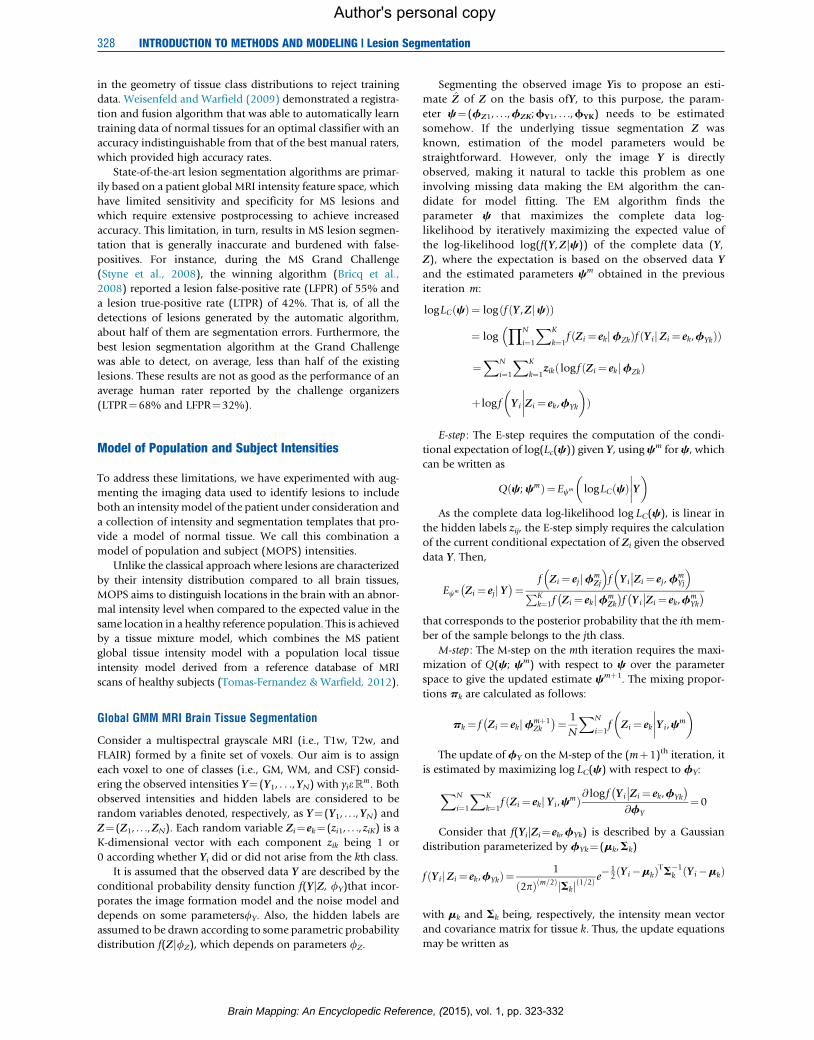
new segmentations and rates themwith a score that summarizes

the performance of the segmentation algorithm. A score of 90

was considered to equal the accuracy of a human rater. MOPS

achieved a score of 84.5, which ranks as the best performing

algorithm over all the 17 lesion segmentation algorithms for

which results have been submitted (Figure 1).

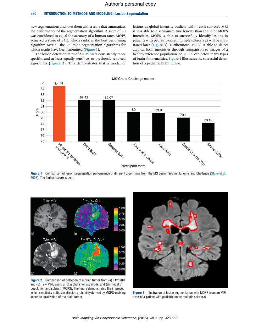
The lesion detection rates of MOPS were consistently more

specific, and at least equally sensitive, to previously reported

algorithms (Figure 2). This demonstrates that a model of

75

Sco

re

Particip

Model of population

and subject

Bricq 2008

Geremia 2011

76

77

78

79

84.46

82.12

MS Grand Ch

82.07

80

81

82

83

84

85

Figure 1 Comparison of lesion segmentation performance of different algor2008). The highest score is best.

1 − f(Yi, Pi, Zi|ψ)

1 − f(Yi, Zi|ψ) T1w MRI

T2w MRI

1.00

0.75

0.50

0.25

0.00

1.00

(a) (c)

(d)(b)

0.75

0.50

0.25

0.00

Figure 2 Comparison of detection of a brain tumor from (a) T1w MRIand (b) T2w MRI, using a (c) global intensity model and (d) model ofpopulation and subject (MOPS). The figure demonstrates the improvedlesion sensitivity of the voxel lesion probability derived by MOPS enablingaccurate localization of the brain tumor.

Brain Mapping: An Encyclopedic Referen

lesions as global intensity outliers within each subject’s MRI

is less able to discriminate true lesions than the joint MOPS

intensities. MOPS is able to successfully identify lesions in

patients with pediatric-onset multiple sclerosis as will be illus-

trated later (Figure 3). Furthermore, MOPS is able to detect

atypical local intensities through comparison to images of a

healthy reference population, so MOPS can detect many types

of brain abnormalities. Figure 4 illustrates the successful detec-

tion of a pediatric brain tumor.

ant team

Souple et al., 2008

Shiee 2010

Garcia-Lorenzo 2011

Anbeek 2004

allenge scores

80 79.979.1

78.19

ithms from the MS Lesion Segmentation Grand Challenge (Styne et al.,

Figure 3 Illustration of lesion segmentation with MOPS from an MRIscan of a patient with pediatric onset multiple sclerosis.

ce, (2015), vol. 1, pp. 323-332

Figure 4 Illustration of tractography of the corticospinal tract in theregion of the brain tumor detected automatically by MOPS. Carefulassessment of the path of the corticospinal tract allows for optimizationof the surgical approach to minimize the risk of loss of function followingsurgery.

INTRODUCTION TO METHODS AND MODELING | Lesion Segmentation 331

Author's personal copy

Conclusion

Lesion segmentation is an important task, regularly carried out

by experts using interactive and semiautomatic segmentation

tools. Automated algorithms for segmentation of lesions have

explored a wide range of techniques and are increasingly effec-

tive for a range of types of pathology. Advances in MS lesion

segmentation enable quantitative and accurate detection of

lesions from high-quality MRI.

See also: INTRODUCTION TO ACQUISITION METHODS:Anatomical MRI for Human Brain Morphometry; Myelin Imaging;INTRODUCTION TO CLINICAL BRAIN MAPPING: DemyelinatingDiseases; MRI in Clinical Management of Multiple Sclerosis;INTRODUCTION TO METHODS AND MODELING: DiffeomorphicImage Registration; Intensity Nonuniformity Correction; NonlinearRegistration Via Displacement Fields; Posterior Probability Maps.

References

Akhondi-Asl, A., & Warfield, S. K. (2013). Simultaneous truth and performance levelestimation through fusion of probabilistic segmentations. IEEE Transactions onMedical Imaging, http://dx.doi.org/10.1109/TMI.2013.2266258.

Anbeek, P., Vincken, K. L., van Osch, M. J., Bisschops, R. H. C., & van der Grond, J.(2004). Automatic segmentation of different-sized white matter lesions by voxelprobability estimation. Medical Image Analysis, 8, 205–215. http://dx.doi.org/10.1016/j.media.2004.06.019.

Ashton, E. A., Takahashi, C., Berg, M. J., Goodman, A., Totterman, S., & Ekholm, S.(2003). Accuracy and reproducibility of manual and semiautomated quantification ofMS lesions by MRI. Journal of Magnetic Resonance Imaging, 17, 300–308. http://dx.doi.org/10.1002/jmri.10258.

Barkhof, F., Simon, J. H., Fazekas, F., Rovaris, M., Kappos, L., de Stefano, N., et al.(2012). MRI monitoring of immunomodulation in relapse-onset multiple sclerosis

Brain Mapping: An Encyclopedic Refere

trials. Nature Reviews. Neurology, 8, 13–21. http://dx.doi.org/10.1038/nrneurol.2011.190.

Bermel, R. A., & Bakshi, R. (2006). The measurement and clinical relevance of brainatrophy in multiple sclerosis. Lancet Neurology, 5, 158–170. http://dx.doi.org/10.1016/S1474-4422(06)70349-0.

Bijar, A., Khayati, R., & Penalver Benavent, A. (2013). Increasing the contrast of thebrain MR FLAIR images using fuzzy membership functions and structural similarityindices in order to segment MS lesions. PloS One, 8, e65469. http://dx.doi.org/10.1371/journal.pone.0065469.

Bricq, S., Collet, C., & Armspach, J. P. (2008). Markovian segmentation of 3D brainMRI to detect multiple sclerosis lesions. In 15th IEEE International Conference onImage Processing (pp. 733–736).

Brinkmann, B. H., Manduca, A., & Robb, R. A. (1998). Optimized homomorphicunsharp masking for MR grayscale inhomogeneity correction. IEEE Transactions onMedical Imaging, 17(2), 161–171. http://dx.doi.org/10.1109/42.700729.

Clarke, L. P., Velthuizen, R. P., Camacho, M. A., Heine, J. J., Vaidyanathan, M.,Hall, L. O., et al. (1995). MRI segmentation: Methods and applications. MagneticResonance Imaging, 13, 343–368.

Cocosco, C. A., Zijdenbos, A. P., & Evans, A. C. (2003). A fully automatic and robustbrain MRI tissue classification method. Medical Image Analysis, 7, 513–527. http://dx.doi.org/10.1016/S1361-8415(03)00037-9.

Commowick, O., Akhondi-Asl, A., & Warfield, S. K. (2012). Estimating a referencestandard segmentation with spatially varying performance parameters: Local MAPSTAPLE. IEEE Transactions on Medical Imaging, 31(8), 1593–1606. http://dx.doi.org/10.1109/TMI.2012.2197406.

Commowick, O., & Warfield, S. K. (2010). Estimation of inferential uncertainty inassessing expert segmentation performance from STAPLE. IEEE Transactions onMedical Imaging, 29(3), 771–780. http://dx.doi.org/10.1109/TMI.2009.2036011.

Datta, S., & Narayana, P. A. (2013). A comprehensive approach to the segmentation ofmultichannel three-dimensional MR brain images in multiple sclerosis.NeuroImage. Clinical, 2, 184–196. http://dx.doi.org/10.1016/j.nicl.2012.12.007.

de Boer, R., Vrooman, H. A., van der Lijn, F., Vernooij, M. W., Ikram, M. A.,van der Lugt, A., et al. (2009). White matter lesion extension to automatic braintissue segmentation on MRI. NeuroImage, 45, 1151–1161.

de Zwart, J. A., Ledden, P. J., van Gelderen, P., Bodurka, J., Chu, R., & Duyn, J. H.(2004). Signal-to-noise ratio and parallel imaging performance of a 16-channelreceive-only brain coil array at 3.0 Tesla. Magnetic Resonance in Medicine, 51(1),22–26. http://dx.doi.org/10.1002/mrm.10678.

Dice, L. R. (1945). Measures of the amount of ecologic association between species.Ecology, 26, 297. http://dx.doi.org/10.2307/1932409.

Filippi, M., Horsfield, M. A., Bressi, S., Martinelli, V., Baratti, C., Reganati, P., et al.(1995). Intra- and inter-observer agreement of brain MRI lesion volumemeasurements in multiple sclerosis. A comparison of techniques. Brain, 118(Pt 6),1593–1600.

Filippi, M., Horsfield, M. A., Tofts, P. S., Barkhof, F., Thompson, A. J., & Miller, D. H.(1995). Quantitative assessment of MRI lesion load in monitoring the evolution ofmultiple sclerosis. Brain, 118(Pt 6), 1601–1612.

Garcıa-Lorenzo, D., Prima, S., Arnold, D. L., Collins, D. L., & Barillot, C. (2011).Trimmed-likelihood estimation for focal lesions and tissue segmentation in multi-sequence MRI for multiple sclerosis. IEEE Transactions on Medical Imaging, 1–13.http://dx.doi.org/10.1109/TMI.2011.2114671.

Geremia, E., Clatz, O., Menze, B. H., Konukoglu, E., Criminisi, A., & Ayache, N. (2011).Spatial decision forests for MS lesion segmentation in multi-channel magneticresonance images. NeuroImage, 57, 378–390.

Grimaud, J., Lai, M., Thorpe, J., & Adeleine, P. (1996). Quantification of MRI lesionload in multiple sclerosis: A comparison of three computer-assisted techniques.Magnetic Resonance Imaging, 14, 495–505.

Guttmann, C. R., Ahn, S. S., Hsu, L., Kikinis, R., & Jolesz, F. A. (1995). The evolution ofmultiple sclerosis lesions on serial MR. AJNR. American Journal of Neuroradiology,16, 1481–1491.

Hadjiprocopis, A., & Tofts, P. (2003). An automatic lesion segmentation method for fastspin echo magnetic resonance images using an ensemble of neural networks.In IEEE XIII workshop on neural networks for signal processing (IEEE Cat.No.03TH8718) (pp. 709–718).

Harmouche, R., Collins, L., Arnold, D., Francis, S., & Arbel, T. (2006). Bayesian MSlesion classification modeling regional and local spatial information. In: Eighteenthinternational conference on pattern recognition (ICPR’06) (pp. 984–987).

Kamber, M., Shinghal, R., Collins, D. L., Francis, G. S., & Evans, A. C. (1995). Model-based 3-D segmentation of multiple sclerosis lesions in magnetic resonance brainimages. IEEE Transactions on Medical Imaging, 14, 442–453. http://dx.doi.org/10.1109/42.414608.

Kamber, M., Louis Collins, D., Shinghal, R., Francis, G. S., & Evans, A. C. (1992).Model-based 3D segmentation of multiple sclerosis lesions in dual-echo MRI data.

nce, (2015), vol. 1, pp. 323-332

332 INTRODUCTION TO METHODS AND MODELING | Lesion Segmentation

Author's personal copy

In: Proceedings of the SPIE: Visualization in biomedical computing 1992, ChapelHill, NJ. vol. 1808 (pp. 590–600).

Kapouleas, I. (1989). Automatic detection of multiple sclerosis lesions in MR brainimages. In: Proceedings of the annual symposium on computer application inmedical care (pp. 739–745).

Kaza, E., Klose, U., & Lotze, M. (2011). Comparison of a 32-channel with a 12-channelhead coil: are there relevant improvements for functional imaging? Journal ofMagnetic Resonance Imaging, 34(1), 173–183. http://dx.doi.org/10.1002/jmri.22614.

Kikinis, R., Guttmann, C. R., Metcalf, D., Wells, W. M., Ettinger, G. J., Weiner, H. L.,et al. (1999). Quantitative follow-up of patients with multiple sclerosis using MRI:Technical aspects. Journal of Magnetic Resonance Imaging, 9, 519–530.

Kikinis, R., Shenton, M. E., Gerig, G., Martin, J., Anderson, M., Metcalf, D., et al. (1992).Routine quantitative analysis of brain and cerebrospinal fluid spaces with MRimaging. Journal of Magnetic Resonance Imaging, 2(6), 619–629.

Kroon, D., Oort, E.V., & Slump, K. (2008). Multiple sclerosis detection in multispectralmagnetic resonance images with principal components analysis. MS LesionSegmentation (MICCAI 2008 Workshop).

Kwan, R. K., Evans, A. C., & Pike, G. B. (1999). MRI simulation-based evaluation ofimage-processing and classification methods. IEEE Transactions on MedicalImaging, 18, 1085–1097. http://dx.doi.org/10.1109/42.816072.

Maltbie, E., Bhatt, K., Paniagua, B., Smith, R. G., Graves, M. M., Mosconi, M. W., et al.(2012). Asymmetric bias in user guided segmentations of brain structures.NeuroImage, 59(2), 1315–1323. http://dx.doi.org/10.1016/j.neuroimage.2011.08.025.

Miller, D. H., Filippi, M., Fazekas, F., Frederiksen, J. L., Matthews, P. M., Montalban, X.,et al. (2004). Role of magnetic resonance imaging within diagnostic criteria formultiple sclerosis. Annals of Neurology, 56, 273–278.

Morra, J., Tu, Z., Toga, A., & Thompson, P. (2008). Automatic segmentation of MSlesions using a contextual model for the MICCAI grand challenge. MS LesionSegmentation, (MICCAI 2008 Workshop).

Neykov, N., Filzmoser, P., Dimova, R., & Neytchev, P. (2007). Robust fitting of mixturesusing the trimmed likelihood estimator. Computational Statistics & Data Analysis,52, 299–308. http://dx.doi.org/10.1016/j.csda.2006.12.024.

Nyul, L. G., & Udupa, J. K. (1999). On standardizing the MR image intensity scale.Magnetic Resonance in Medicine, 42, 1072–1081.

Paty, D. W., & Li, D. K. (1993). Interferon beta-1b is effective in relapsing-remittingmultiple sclerosis. II. MRI analysis results of a multicenter, randomized, double-blind, placebo-controlled trial. UBC MS/MRI Study Group and the IFNB MultipleSclerosis Study Group. Neurology, 43(4), 662–667.

Prastawa, M., Bullitt, E., & Ho, S. (2004). A brain tumor segmentation framework basedon outlier detection. Medical Image Analysis, 8, 275–283.

Shah, M., Xiao, Y., Subbanna, N., Francis, S., Arnold, D. L., Collins, D. L., et al. (2011).Evaluating intensity normalization on MRIs of human brain with multiple sclerosis.Medical Image Analysis, 15(2), 267–282. http://dx.doi.org/10.1016/j.media.2010.12.003, pii: S1361-8415(10)00133-7.

Shepherd, T., Prince, S. J., & Alexander, D. C. (2012). Interactive lesion segmentationwith shape priors from offline and online learning. IEEE Transactions on MedicalImaging, 31, 1698–1712. http://dx.doi.org/10.1109/TMI.2012.2196285.

Shiee, N., Bazin, P. L., Ozturk, A., Reich, D. S., Calabresi, P. A., & Pham, D. L. (2010). Atopology-preserving approach to the segmentation of brain images with multiplesclerosis lesions. NeuroImage, 49, 1524–1535.

Sled, J. G., Zijdenbos, A. P., & Evans, A. C. (1998). A nonparametric method forautomatic correction of intensity nonuniformity in MRI data. IEEE Transactions onMedical Imaging, 17, 87–97. http://dx.doi.org/10.1109/42.668698.

Souple, J., Lebrun, C., Ayache, N., & Malandain, G. (2008) An Automatic Segmentationof T2-FLAIR Multiple Sclerosis Lesions. MS Lesion Segmentation (MICCAI 2008workshop).

Styne, M., Lee, J., Chin, B., Chin, M.S., Commowick, O., Tran, H., et al. (2008). 3DSegmentation in the Clinic: A Grand Challenge II, MS Lesion Segmentation(MICCAI 2008 Workshop).

Thompson, D. K., Wood, S. J., Doyle, L. W., Warfield, S. K., Egan, G. F., & Inder, T. E.(2009). MR-determined hippocampal asymmetry in full-term and preterm neonates.Hippocampus, 19(2), 118–123. http://dx.doi.org/10.1002/hipo.20492.

Tomas-Fernandez, X., & Warfield, S. K. (2012). Population intensity outliers or a newmodel for brain WM abnormalities. In: Ninth IEEE international symposium onbiomedical imaging (ISBI) (pp. 1543–1546), IEEE.

Udupa, J. K., Wei, L., Samarasekera, S., Miki, Y., van Buchem, M. A., & Grossman, R. I.(1997). Multiple sclerosis lesion quantification using fuzzy-connectednessprinciples. IEEE Transactions on Medical Imaging, 16, 598–609. http://dx.doi.org/10.1109/42.640750.

Brain Mapping: An Encyclopedic Referen

Van Leemput, K., Maes, F., Vandermeulen, D., Colchester, A., & Suetens, P. (2001).Automated segmentation of multiple sclerosis lesions by model outlier detection.IEEE Transactions on Medical Imaging, 20, 677–688.

Van Leemput, K., Maes, F., Vandermeulen, D., & Suetens, P. (1999). Automatedmodel-based tissue classification of MR images of the brain. IEEE Transactions onMedical Imaging, 18, 897–908. http://dx.doi.org/10.1109/42.811270.

Vannier, M. W., Butterfield, R. L., Jordan, D., Murphy, W. A., Levitt, R. G., & Gado, M.(1985). Multispectral analysis of magnetic resonance images. Radiology, 154(1),221–224. http://dx.doi.org/10.1148/radiology.154.1.3964938.

Vannier, M. W., Butterfield, R. L., & Jordan, D. (1985). Multispectral analysis ofmagnetic, resonance images. Radiology, 154, 221–224.

Wack, D. S., Dwyer, M. G., Bergsland, N., Di Perri, C., Ranza, L., Hussein, S., et al.(2012). Improved assessment of multiple sclerosis lesion segmentation agreementvia detection and outline error estimates. BMC Medical Imaging, 12, 17. http://dx.doi.org/10.1186/1471-2342-12-17.

Warfield, S. K., Kaus, M., Jolesz, F. A., & Kikinis, R. (2000). Adaptive, templatemoderated, spatially varying statistical classification. Medical Image Analysis, 4,43–55.

Warfield, S., Dengler, J., Zaers, J., Guttmann, C. R., Wells, W. M., 3rd., Ettinger, G. J.,et al. (1995). Automatic identification of gray matter structures from MRI to improvethe segmentation of white matter lesions. Journal of Image Guided Surgery, 1(6),326–338. http://dx.doi.org/10.1002/(SICI)1522-712X.

Warfield, S. K., Zou, K. H., & Wells, W. M. (2004). Simultaneous truth and performancelevel estimation (STAPLE): An algorithm for the validation of image segmentation.IEEE Transactions on Medical Imaging, 23, 903–921. http://dx.doi.org/10.1109/TMI.2004.828354.

Wei, X., Guttmann, C. R., Warfield, S. K., Eliasziw, M., & Mitchell, J. R. (2004). Has yourpatient’s multiple sclerosis lesion burden or brain atrophy actually changed?Multiple Sclerosis, 10, 402–406.

Wei, X., Warfield, S. K., Zou, K. H., Wu, Y., Li, X., Guimond, A., et al. (2002).Quantitative analysis of MRI signal abnormalities of brain white matter with highreproducibility and accuracy. Journal of Magnetic Resonance Imaging, 209,203–209. http://dx.doi.org/10.1002/jmri.10053.

Weisenfeld, N. I., & Warfield, S. K. (2009). Automatic segmentation of newborn brainMRI. NeuroImage, 47, 564–572. http://dx.doi.org/10.1016/j.neuroimage.2009.04.068.

Weisenfeld, N. I., & Warfield, S. K. (2004). Normalization of joint image-intensitystatistics in MRI using the Kullback–Leibler divergence. In Proceedings of the 2004IEEE international symposium on biomedical imaging: From nano to macro,Arlington, VA, April 15–18, 2004.

Wells, W. M., Grimson, W. L., Kikinis, R., & Jolesz, F. A. (1996).Adaptive segmentation of MRI data. IEEE Transactions on Medical Imaging, 15,429–442.

Wels, M., Huber, M., & Hornegger, J. (2008). Fully automated segmentation of multiplesclerosis lesions in multispectral MRI. Pattern Recognition and Image Analysis, 18,347–350. http://dx.doi.org/10.1134/S1054661808020235.

Younis, A. A., Soliman, A. T., Kabuka, M. R., & John, N. M. (2007). MS lesionsdetection in MRI using grouping artificial immune networks. In IEEE 7thinternational symposium on bioinformatics and bioengineering (pp. 1139–1146).

Zijdenbos, A. P., Dawant, B. M., Margolin, R. A., & Palmer, A. C. (1994). Morphometricanalysis of white matter lesions in MR images: Method and validation. IEEETransactions on Medical Imaging, 13, 716–724. http://dx.doi.org/10.1109/42.363096.

Zijdenbos, A. P., Forghani, R., & Evans, A. C. (2002). Automatic ‘pipeline’ analysis of3-D MRI data for clinical trials: Application to multiple sclerosis. IEEE Transactionson Medical Imaging, 21, 1280–1291.

Relevant Websites

http://brainweb.bic.mni.mcgill.ca/brainweb/selection_ms.html – BrainWeb LesionSimulator.

http://www.spl.harvard.edu/publications/item/view/1180 – Warfield/Kaus database.http://crl.med.harvard.edu/software – STAPLE validation software.http://martinos.org/qtim/miccai2013/ – Multimodal Brain Tumor Segmentation.http://www.sci.utah.edu/�prastawa/software.html – Brain Tumor Simulator.http://www.ia.unc.edu/MSseg/ – Multiple Sclerosis Lesion Segmentation Grand

Challenge.

ce, (2015), vol. 1, pp. 323-332