thinning-stable point processes as a model for bursty ...aila/statdas.pdf · stability and discrete...

Stability and discrete stabilityParameter inference

Thinning-stable point processes as a model forbursty spatial data

Sergei Zuyev

Chalmers University of Technology, Gothenburg, Sweden

Smogen, Aug. 29th 2014

Sergei Zuyev Thinning-stable point processes as a model for bursty spatial data


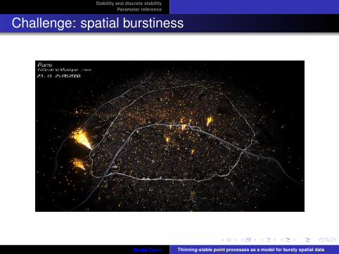
Challenge: spatial burstiness



Stability

DefinitionA random vector ξ (generally, a random element on a convex cone) iscalled strictly α-stable (notation: StαS) if for any t ∈ [0, 1]

t1/αξ′ + (1− t)1/αξ′′D= ξ, (1)

where ξ′ and ξ′′ are independent copies of ξ.

Stability and CLT

Only StαS vectors ξ can appear as a weak limitn−1/α(ζ1 + · · ·+ ζn) =⇒ ξ.



DαS point processes

Definition

A point process Φ (or its probability distribution) is called discreteα-stable or α-stable with respect to thinning (notation DαS), if for any0 ≤ t ≤ 1

t1/α ◦ Φ′ + (1− t)1/α ◦ Φ′′D= Φ ,

where Φ′ and Φ′′ are independent copies of Φ and t ◦ Φ isindependent thinning of its points with retention probability t.



Discrete stability and limit theorems

Let Ψ1,Ψ2, . . . be a sequence of i. i. d. point processes andSn =

∑ni=1 Ψi. If there exists a PP Φ such that for some α we have

n−1/α ◦ Sn =⇒ Φ as n→∞

then Φ is DαS.

CLTWhen intensity measure of Ψ is σ-finite, then α = 1 and Φ is aPoisson processes. Otherwise, Φ has infinite intensity measure –bursty



DαS point processes and StαS random measures

Cox process

Let ξ be a random measure on the space X. A point process Φ on Xis a Cox process directed by ξ, when, conditional on ξ, realisations ofΦ are those of a Poisson process with intensity measure ξ.



Characterisation of DαS PP

TheoremA PP Φ is a (regular) DαS iff it is a Cox process Πξ with a StαSintensity measure ξ, i.e. a random measure satisfying

t1/αξ′ + (1− t)1/αξ′′D= ξ .

Its p.g.fl. is given by

GΦ[u] = E∏xi∈Φ

u(xi) = exp{−∫M1

〈1− u, µ〉ασ(dµ)}, 1− u ∈ BM

for some locally finite spectral measure σ on the set M1 of probabilitymeasures.

DαS PPs exist only for 0 < α ≤ 1 and for α = 1 these are Poisson.



Sibuya point processes

Definition

A r.v. γ has Sibuya distribution, Sib(α), if

gγ(s) = 1− (1− s)α, α ∈ (0, 1) .

It corresponds to the number of trials to get the first success in aseries of Bernoulli trials with probability of success in the kth trialbeing α/k.

Sibuya point processes

Let µ be a probability measure on X. The point process Υ on X iscalled the Sibuya point process with exponent α and parametermeasure µ if Υ(X) ∼ Sib(α) and each point is µ-distributedindependently of the other points. Its distribution is denoted bySib(α, µ).



Examples of Sibuya point processes

Figure : Sibuya processes: α = 0.4, µ ∼ N (0, 0.32I)



DαS point processes as cluster processes

Theorem Davydov, Molchanov & Z’11

Let M1 be the set of all probability measures on X. A regular DαSpoint process Φ can be represented as a cluster process with

Poisson centre process on M1 driven by intensity measure σ;Component processes being Sibuya processes Sib(α, µ),µ ∈M1.



Statistical Inference for DαS processes

We assume the observed realisation comes from a stationary andergodic DαS process without multiple points.

Such processes are characterised by:λ – the Poisson parameter: mean number of clusters per unitvolumeα – the stability parameter

A probability distribution σ0(dµ) on M1 (the distribution of theSibuya parameter measure)



Construction

1 Generate a homogeneous Poisson PP∑

i δyi of centres ofintensity λ;

2 For each yi generate independently a probability measure µi

from distribution σ0;3 Take the union of independent Sibuya clusters Sib(α, µi( • − yi)).



Example of DαS point process

Figure : λ = 0.4, α = 0.6, σ0 = δµ, where µ ∼ N (0, 0.32I)



Estimation of µEstimation of λ and α

Parameters to estimate

Consider the case when all the clusters have the same distribution,so that σ0 = δµ for some µ ∈M1.

We always need to estimate λ and α, often also µ.

We consider three possible cases for µ:µ is already knownµ is unknown but lies in a parametric class (e.g. µ ∼ N (0, σ2I) orµ ∼ U(Br(0)))µ is totally unknown




Estimation of µ

IdeaIdentifying a big cluster in the dataset and using it to estimate µ.

How to distinguish clusters in the configuration? How to identify atleast the biggest clusters?

Interpreting data as a mixture modelExpectation-Maximisation algorithmBayesian Information Criterion




Estimation of µ



Interpreting data as a mixture model

Expectation-Maximisation algorithmBayesian Information Criterion




Estimation of µ



Interpreting data as a mixture modelExpectation-Maximisation algorithm

Bayesian Information Criterion




Estimation of µ



Interpreting data as a mixture modelExpectation-Maximisation algorithmBayesian Information Criterion




Example: gaussian spherical clusters, 2D case

(a) Original process (b) Clustered process

Figure : DαS process with Gaussian clusters: λ = 0.5, α = 0.6, covariancematrix 0.12I. mclust R-procedure with Poisson noise.




Estimation of µ

After we single out one big cluster:

we estimate µ using kernel density or we just use the samplemeasure

if µ is in a parametric class we estimate the parameters




Overlaping clusters - heavy thinning approach

Figure : λ = 0.4, α = 0.6, µx ∼ N (x, 0.52I)




Estimation of λ and α

When µ is known or have already been estimated, we suggest these

Estimation methods for λ and α1 via void probabilities

2 via the p.g.f. of the counts distribution




Estimation of λ and α

When µ is known or have already been estimated, we suggest these

Estimation methods for λ and α1 via void probabilities2 via the p.g.f. of the counts distribution




Void probabilities for DαS point processes

The void probabilities (which characterise the distribution of a simplepoint process) are given by

P{Φ(B) = 0} = exp{− λ

∫Aµ(B)α dx

}.




Estimation of void probabilities

Unbiased estimator for the void probability function

Let {xi}ni=1 ⊆ A a sequence of test points and ri = dist(xi, supp Φ), then

G(r) =1n

n∑i=1

1I{ri>r}

is an unbiased estimator for P{Φ(Br(0)) = 0}.

Then α and λ are estimated by the best fit to this curve.




Example: uniformly distributed clusters, 1D case

Figure : λ = 0.3, α = 0.7, µ ∼ U(B1(0)), |A| = 3000

Estimated values: λ = 0.29, α = 0.68. Requires bigdata!




Void probabilities for thinned processes

p.g.fl. of DαS processes

GΦ[h] = exp{−∫S〈1− h, µ〉ασ(dµ)

}, 1− h ∈ BM(X).

p.g.fl. of a p-thinned point process

Gp◦Φ[h] = exp{−pα

∫S〈1−h, µ〉ασ(dµ)

}, p ∈ [0, 1], 1−h ∈ BM(X).

σ({µ(· − x), x ∈ B}) = λ · |B| =⇒ αnew = α, λnew = λ · pα.




Estimation via thinned processThere is no need to simulate p-thinning!Let rk be the distance from 0 to the k-th closest point in theconfiguration.

r1

r30r2




Estimation via thinned process

P{(p ◦ Φ)(Br(0)) = 0}

=

Φ∑k=1

P{“the closest survived point is the k-th”}P{rk > r}

=

Φ∑k=1

p(1− p)k−1P{rk > r}


Let {xi}ni=1 ⊆ A a sequence of test points and ri,k be the distance from

xi to its k-closest point of supp Φ. Then

G(r) =1n

n∑i=1

∑k=0

p(1− p)k−1 1I{ri,k>r}

is an unbiased estimator for P{Φ(Br(0)) = 0}.




Estimation via thinned process

P{(p ◦ Φ)(Br(0)) = 0}

=

Φ∑k=1

P{“the closest survived point is the k-th”}P{rk > r}

=

Φ∑k=1

p(1− p)k−1P{rk > r}


Let {xi}ni=1 ⊆ A a sequence of test points and ri,k be the distance from

xi to its k-closest point of supp Φ. Then

G(r) =1n

n∑i=1

∑k=0

p(1− p)k−1 1I{ri,k>r}

is an unbiased estimator for P{Φ(Br(0)) = 0}.Sergei Zuyev Thinning-stable point processes as a model for bursty spatial data



Example: uniform clusters, 1D case

Figure : Estimation of v.p. of the thinned process for a process generatedwith λ = 0.3, α = 0.7, µ ∼ U(B1(0)), |A| = 1000

Estimated values: λ = 0.29, α = 0.72Sergei Zuyev Thinning-stable point processes as a model for bursty spatial data



Counts distribution

Putting u(x) = 1− (1− s) 1IB(x) with s ∈ [0, 1], in the p.g.fl. expression,we get the p.g.f. of the counts Φ(B) for any set B:

ψΦ(B)(s) := E[sΦ(B)] = exp{− (1− s)α

∫Sµ(B)ασ(dµ)

}. (2)

It is a heavy-tailed distribution with P{Φ(B) > x} = L(x) x−α, where Lis slowly-varying.




Estimation via counts distribution

The empirical p.g.f. is then

ψnΦ(B)(s) :=

1n

n∑i=1

sΦ(Bi) ∀s ∈ [0, 1],

where Bi, i = 1, . . . , n, are translates of a fixed referece set B and it isan unbiased estimator of ψΦ(B). It is then fitted to (2) for a range of sestimating λ and α.We also tried the Hill plot from extremal distributions inference toestimate α, but the results were poor!




Conclusions

Simulation studies looked at the bias and variance in the extimation ofα, λ in different situations:

Big sample – moderate sampleOverlapping clusters (large λ) – separate clusters (small λ)Heavy clusters (small α) – moderate clusters (α close to 1)




Best methods

The simplest void probabilities method is prefered for largedatasets or for moderate datasets with separated clusters. It bestestimates α, but in the latter case λ is best estimated by countsp.g.f. fitting.

λ is best estimated by void probabilities with thinning methodwhich produces best estimates in all the situations apart frommoderate separated clusters. But it is also more computationallyexpensive.As common in modern Statistics, all methods should be tried andconsistency in estimated values gives more trust to the model.




Best methods

The simplest void probabilities method is prefered for largedatasets or for moderate datasets with separated clusters. It bestestimates α, but in the latter case λ is best estimated by countsp.g.f. fitting.λ is best estimated by void probabilities with thinning methodwhich produces best estimates in all the situations apart frommoderate separated clusters. But it is also more computationallyexpensive.

As common in modern Statistics, all methods should be tried andconsistency in estimated values gives more trust to the model.




Best methods

The simplest void probabilities method is prefered for largedatasets or for moderate datasets with separated clusters. It bestestimates α, but in the latter case λ is best estimated by countsp.g.f. fitting.λ is best estimated by void probabilities with thinning methodwhich produces best estimates in all the situations apart frommoderate separated clusters. But it is also more computationallyexpensive.As common in modern Statistics, all methods should be tried andconsistency in estimated values gives more trust to the model.




Fete de la Musique data

Figure : Estimated α = 0.17− 0.28 depending on the way base stationsrecords are extrapolated to spatial positions of callers




Generalisations

For the Paris data we observed a bad fit of cluster size to Sibuyadistribution. Possible cure:

F-stable point processes when thinning is replaced by more generalsubcritical branching operation. Multiple points are now also allowed.




References

1 Yu. Davydov, I. Molchanov and SZ Stability for randommeasures, point processes and discrete semigroups,Bernoulli, 17(3), 1015-1043, 2011

2 espi, B. Spinelli and SZ Inference for discrete stable pointprocesses (under preparation)

3 G. Zanella and SZ F-stable point processes (underpreparation)




Thank you!

Questions?Sergei Zuyev Thinning-stable point processes as a model for bursty spatial data

thinning-stable point processes as a model for bursty ...aila/statdas.pdf · stability and discrete...

Documents