thinned arrays using genetic algorithms

7/30/2019 Thinned Arrays Using Genetic Algorithms

http://slidepdf.com/reader/full/thinned-arrays-using-genetic-algorithms 1/7

IEEE TRANSACTIONS ON ANTENNAS AND PROPAGATION, VOL. 42, NO. 7, JULY 1994 993

Thinned Arrays Using Genetic AlgorithmsRandy L. Haupt, Senior Member, IEEE

Abstract-Large arrays are difficult to thin in order to ob-

tain low sidelobes. lhditional statistical methods of aperiodicarray synthesis fall far short of optimum configurations. Tradi-

tional optimization methods are not well suited for optimizing a

large number of parameters or discrete parameters. This paper

presents how to optimally thin an array using genetic algorithms.

The genetic algorithm determines which elements are turned off

in a periodic array to yield the lowest maximum relative sidelobe

level. Simulation results for 200 element linear arrays and 200

element planar arrays are shown. The arrays are thinned to

obtain sidelobe levels of less than -20 dB. The linear arrays are

also optimized over both scan angle and bandwidth.

I. INTRODUCTION

PERIODIC arrays generate a low sidelobe amplitudeA aper by strategically positioning equally weighted el-

ements. Simple analytical methods for deriving the element

positions to obtain a desired sidelobe level are not available

[l ]. Instead, most aperiodic array synthesis methods try to

relate the element density at a region of the array to the

amplitude density of a low sidelobe amplitude taper for the

same size aperture [2]. The element density is greatest at the

center of the array and gradually decreases toward the edges. In

general, sidelobes close to the main beam decrease, while those

far from the main beam increase [3] (which is usually quite

acceptable). Aperiodic array synthesis methods either target a

rms sidelobe level or a maximum relative sidelobe level with

a given probability [4].

Thinning an array means turning off some elements in

a uniformly spaced or periodic array to create a desired

amplitude density across the aperture. An element connected

to the feed network is “on”, and an element connected toa matched or dummy load is ‘‘off ’. Thinning an array to

produce low sidelobes is much simpler than the more general

problem of nonuniform spacing the elements. Nonuniform

spacing has an infinite number of possibilities for placement of

the elements. Thinning has 2Q possible combinations, where Q

is the number of array elements. If the array is symmetric, then

the number of possibilities is substantially smaller. Thinning

may also be thought of as a quantized amplitude taper where

the amplitude at each element is represented by one bit.

Thinning a large array for low sidelobes involves checking

a rather large number of possibilities in order to find the best

thinned aperture. Exhaustive checking of all possible element

combinations is only practical for small arrays [5]. Most

optimization methods (including down-hill simplex, Powell’s

method, and conjugate gradient) are not well suited for thin-

Manuscript received September 21, 1993; revised February 14, 1994.

The author is with th e Department of Electrical Engineering, USAF

IEEE Log Number 9402866.

Academy, CO 80840 USA.

ning arrays. They can only optimize a few continuous variables

and get stuck in local minima [6]. Also, these methodswere developed for continuous parameters, whereas the array

thinning problem involves discrete parameters. Dynamic pro-

gramming can optimize a large parameter set (many elements),

but it is vulnerable to local minima [ l l ]

Simulated annealing and genetic algorithms [7] are opti-

mization methods that are well suited for thinning arrays.

There is no limit to the number of variables that can be

optimized. Although quite s low, these algorithms can handle

very large arrays. These methods are global in that they have

random components that test for solutions outside the current

minimum, while the algorithm converges. The global nature of

the algorithms and the lack of derivative information causes

them to converge very slowly compared to other nonglobal

methods.

Ruf used simulated annealing to optimize low-redundancy

linear arrays [8]. These antennas are used in radio astronomy

to estimate scene radiance. Astronomers are interested in

designing arrays that properly sample the spatial distribution

they observe. His approach optimized much larger linear array

configurations than ever before.

The purpose of this paper is to find a thinned array that

produces the lowest maximum relative sidelobe level (rsll). A

genetic algorithm is used to numerically optimize both linear

and planar arrays [9]. Genetic algorithms are modeled after

genetic recombination and evolution. The algorithms encode

parameters in binary strings called genes and perform the ge-

netic operations of reproduction, crossover, natural selection,

and mutation to arrive at the optimum solution. These algo-

rithms arrive at better thinning configurations for arrays thanprevious optimization attempts or statistical attempts. Other

optimization methods cannot be applied to large arrays, while

statistical methods cannot find optimum solutions. Excellent

results are obtained using genetic algorithms to optimize linear

arrays and planar arrays with 200 elements. The linear arrays

can be optimized for maximum relative sidelobe levels less

than -20 dB over a range of scan angles and frequencies.

11. THE GENETIC LGORITHM

The goal of the genetic algorithm is to find a set of

parameters that minimizes the output of a function. Genetic

algorithms differ from most optimization methods, because

they have the following charactreistics [101.

1) They work with a coding of the parameters, not theparameters themselves.

2) They search from many points instead of a single point.

3) They don’t use derivatives.

4) They use random transition rules, not deterministic rules.

0018-926)(/94$04.00 0 1994 IEEE



994

set parameters A

Fig. 1. Flow chart of a genetic algorithm.

Fig. 1 is a flow chart of a genetic algori thm. The fol-

lowing paragraphs describe the details of each step in the

algorithm. Steps are labeled as A through F for easy refer-ence.

Values for all the parameters are represented by a binary

code (step A). Each encoded parameter is placed side by

side to form a long binary string called a gene. Every gene

has an associated output corresponding to the function evalu-

ated at the quantized parameters. Thus, the genetic algorithm

has a finite, but possibly very large, number of parameter

combinations to check. A gene with N ; B-bit parameters

has a total of Z N B possible genes. If the parameters are

continuous, then the genetic algorithm limits performance due

to quantization errors associated with the binary encoding

of the parameters. On the positive side, genetic algorithms

are ideally suited for optimization of functions with discrete

parameters.

A thinned array has discrete parameters. One bit represents

the element state as “on” = 1 or “off” =0. For example,

a six element array may be represented by 101101, where

elements 2 and 5 are turned “off.” Assuming the linear array

is symmetric about its center allows the 2N element array to

be represented by a gene with N bits. Our six-element array

example can then be represented by the gene 101. The fitness

associated with this gene is the maximum relative sidelobe

level (rsll) of its associated far-field pattern. The function in

this paper is the relative far-field pattern of an array of point

sources. Its output to be minimized is the maximum rsll. The

parameters affecting the output are whether an antenna element

is on or off.

Genetic algorithms model genetic recombination and evolu-

tion in nature [lo]. As in nature, the gene is the basic buildingblock. Genetic algorithms start with a random sampling of the

output space. Many of the genes from this list have terrible

maximum rsll’s. Genes that produce a superior output survive,

while genes that produce a weak output die off. For instance,

consider the list of eight randomly generated genes (step B)

in Table I.

IEEE TRANSACTIONS ON ANTENNAS AND PROPAGATION, VOL. 42 , NO . I . JULY 1994

TABLE I

EIGHTRANDOMLYENERATEDENESWITH ASSOCIATEDSLL

Gene Code

1111011001

1111111001

1111011110

1101111 001

1111011101

11101 10010

1111110010

1011110101

Max rsll (dB)

-9.06

-14.08

-12.13

-9.71

-11.09

-7.31

-12.76

-8.70

These genes represent a 20-element array of isotropic pointsources spaced $ apart. Each gene has an associated rsll

calculated from

where

2N = number of elements in the array. K, = amplitude weight of element n =

d = spacing between elements.

4 = angle measured from line passing through antenna

elements.6 = steering phase = -27rdu,.

e l p a t ( u ) = element pattern.

e , = constant.

FF,,, = peak of main beam.

The region of U for which F F is valid excludes the main

beam. The first null for a uniform array occurs at U =A.Thinning an array causes the null to move, so a constant, eo ,

is needed in the formula to adjust for the first null location.

Which of these output values from Table I are fit enough to

survive? First, let’s rank them from best to worst, as shown in

Table I1 (step C). The most common suitability criterion is to

discard (step D) the bottom half and keep the top half of the

list. Note, however, that only gene 2 has a rsll of less than - 3

dB. Another possible criterion is to discard any gene that hasa rsll of less than -13 dB. This limitation speeds convergence

of the algorithm. Since a fully populated array has a rsll of

slightly less than -13 dB, only one of these genes shows any

improvement over a nonthinned array.

After the “natural” selection takes place, the genes mate

(step E) to produce offspring. Mating takes place by pairing

U = cos(4 ) .



HAUPT: THINNED ARRAYS USING GENETIC ALGORITHMS

Code

11111 11*001

1111110*010

111 101111*0

111101110*1

11 111 11*010

1111 10*001

111101 11 1*1

111101 110*0

995

Ma x rsll (dB)

-14.08

-12.76

-12.13

-11.09

-

-

-

-

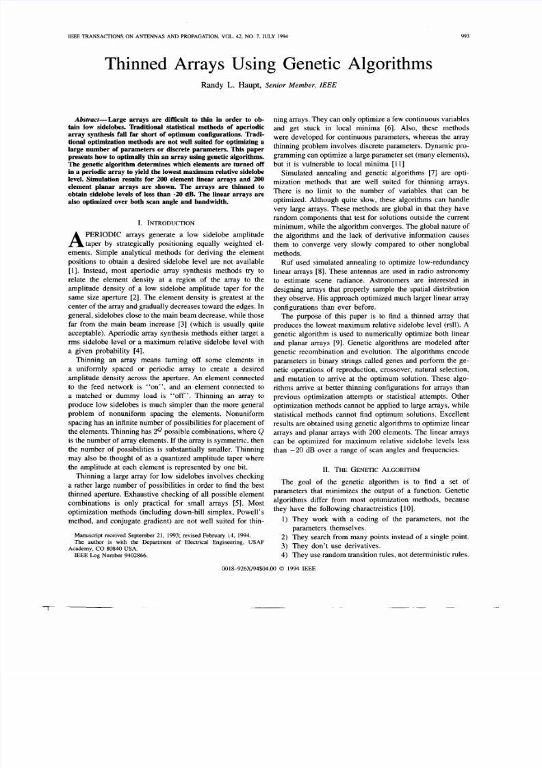
TABLE I1

GENB RANKED ACCORDINGO FITNESS

Gene Code

1111111001

1111110010

1111011110

1111011101

1101111001

1111011001

1011110101

1110110010

Ma x rsll (dB)

-14.08

-12.76

-12.13

-11.09

-9.71

-9.06

-8.70

-7.31

Fig. 2. Two genes mating. A random crossover point is selected for twoparent genes. Offspring are created by swapping the bits to the right of the

crossover point.

the surviving genes. Once paired, their offspring consist of

genetic material from both parents. Fig. 2 shows gene 2 mating

with gene 7 to produce genes 9 and 10.The random crossover

point is between bits selected for each pair of genes. One of

the offspring consists of the bit sequence from the left side

of the crossover point of parent A and the bit sequence from

the right side of the crossover point of parent B. Likewise,

the other offspring consists of the bit sequence from the left

side of the crossover point of parent B and the bit sequence

from the right side of the crossover point of parent A. The top

four genes in Table 111 survived natural selection and became

parents of the bottom four genes. Genes 9 and 10are offspring

of genes 2 and 7, and genes 11 and 12 are offspring of genes

3 and 5.

One last step is to introduce a random mutation in the list

of genes (step F). A mutation changes a zero to a one or a

one to a zero. In this example only one bit in all the genes

is mutated in each iteration. The mutation helps the algorithm

avoid a local minimum.The process starts over again with the parents and the

offspring (step C ).Table IV shows the parents and offspring

(with a mutation) of Table I11 listed in order from best to worst.

Note that bit 6 in gene 10mutated in Table IV. Gene 10 had an

output of -11.73 dB until its sixth bit mutated. The mutation

caused the output to drop to -9.43 dB. Mutation usually

TABLE IU

OFFSPRING2 AND 7 BEGAT AN D 10, AN D 3 AND 5 BEGAT 1 AND 12).THE OP FOUR GENESARE THE PARENTS, AND THE BOTTOMOU R RE THE

TH E OFFSPRING MAXIMUMSLL HAVE NOT YET BEEN EVALUATED.THE *'S INDICATERANDOMCROSSOVER POINTS

Gene

2

7

3

5

9

10

11

12

THESE RE THE PARENTSND OFFSPRINGANKEDAFTERMUTATIONF BlT 6 IN GENE10

Gene

9

2

7

3

11

12

5

10

Code

1111111010

1111111001

1111110010

1111011110

1111011101

1111011100

1111011101

111 1100001

Max rsll (dB)

-14.66

-14.08

-12.76

-12.13

-12.01

-11.89

-11.09

-9.43

doesn't improve the solution. It is a very necessary part of

genetic algorithms, though. Without it, genetic algorithms are

more likely to get stuck in a local minimum. Natural selection,

mating, and mutation will take place with these genes. The

algorithm continues this process until a suitable stopping point

is reached. Eventually, all the genes will be identical except

for the single mutated gene.

The person programming the genetic algorithm has many

variables to control and trade-offs to consider. For instance:

1) Number of bits that represent a parameter. More bits

give greater accuracy but slow convergence. This is

not an issue with array thinning, since each element is



996

-5

-10-mD

C

0 15--m_c_m -20

represented by one bit. A continuous parameter, such as

an element amplitude weight, however, is sensitive to

quantization.

2) Number of genes in the initial random population. More

genes provide a better sampling of the solution space

but slow convergence.

3) Generating the random list . The type of probability

distribution and weighting of the parameters has a sig-

nificant impact on the convergence time.

4) Natural selection. Several methods are available for

deciding which genes to discard.

5) Pairing the genes for mating. Genes may be paired from

top to the bottom of the list, randomly, best with worst,

etc.

6) Number of mutations. Mutations guard against the al-

gorithm getting stuck in a local minimum but slow

convergence.

7) When does the algorithm converge? Determining a stop-

ping point for the algorithm is difficult. Eventually the

natural selection and mating processes will cause all the

genes to be the same, except for the mutated gene.

The above tradeoffs will be referenced by Roman numerals

in the next section. All these considerations and more makegenetic algorithms an interesting numerical method to explore.

In general, I found the genetic algorithm converged well for a

variety of options mentioned in the tradeoffs. The main impact

of the options is on convergence speed.

-

-

111. OPTIMALLYHINNED RRAYS

The previous section gave a step-by-step description of how

the algorithm worked for a small array. Applying genetic

programming to optimizing small arrays is overkill, because

small arrays can be optimized by looking at every possible

thinning combination and selecting the best one. This section

looks at more realistic applications of genetic algorithms to

array thinning. Results for optimizing the rsll of a 200-element

linear array and a 200-element planar array are presented. Itis impractical to optimize these arrays by examining every

possible combination of thinning.

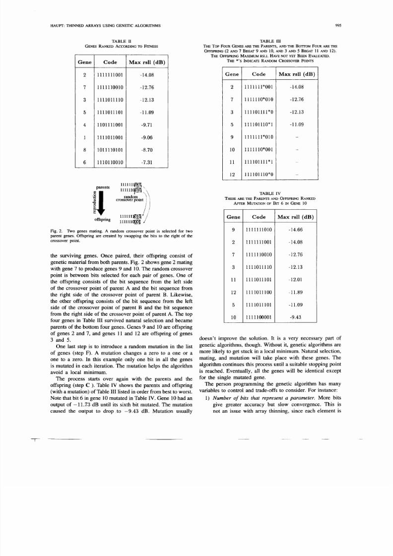
Fig. 3(a) is the far-field pattern of a thinned array of 200

isotropic point sources. The element status (on or om for

half the array is shown at the top of the picture. The top

left 1 is the first element to the right of array center, and the

bottom right 1 is at the right edge. The left side of the array

is the mirror image of the right. In this case a 77% filled

array produced a maximum rsll of -22.09 dB. The aperture

size is approximately lOOX, and the gain is approximately

21.9 dB (gain? NtG,, where MNt =number of elements

turned on and G, =the element gain [111). Only genes with

a maximum rsll of -1 3 dB or better were allowed to survive

(see 4 above). The initial list of 200 random genes (see 2)

was weighted so that the center elements were more likely to

be turned on than the elements towards the edge (see 3 ) . This

weighting significantly speeds convergence of the algorithm.

Several sidelobes distributed throughout the far-field pattern

nearly touch the -22.09 dB maximum rsll. Genes were paired

from best to worst (see 5), and two mutations occurred every

I

IEEE TRANSACTIONS ON ANTENNAS AND PROPAGATION, VOL. 42, NO. 7, JULY 1994

#elements=200

77% illed

isotropic element pattern

max sll=-22.09

d 4 . 5

11111111111111111111111111111111111111111111001111

10011111110111110100001010111001001011100010101101

0

-5

-10-mD

c

a,

0 -15--._L

3 20

#elements=200

sin(phi) element pattern

max sll=-23.69

- 75% filled

d=0.5

-

U

(b )

Fig. 3. (a) F ar-field pattern of a thinned array of 200 isotropic point sources.(b) Far-field pattern of a thinned array of 200 sources having a I sin dl elementpattern.

iteration (see 6). I stopped the algorithm after thirty iterations

(see 7). Statistical aperiodic array theory predicts that over

1000 elements are needed to obtain a -22-dB maximum rsll

with 90% probability for a l OOX aperture [I]. The optimum

array designed here has low sidelobes and high gain, and is

practical to build.

Fig. 3(b) is the far-field pattern of a thinned array of 200

point sources with a I sin q5I element pattern. In this case, a

75% filled array produced a maximum rsll of -23.69 dB.

Optimizing on the array with an element pattern produced

results 1.6 dB better than the isotropic element array. The

thinning for these two examples are quite different even though

both are 200-element arrays.

Thinning the array of directional elements yields better

results at broadside than thinning an array of isotropic point



HAUPT THINNED ARRAYS USING GENETIC ALGORITHMS

-5

-10

mU

.--15--m=

991

-

-

11111111111111111111111111111111111111111111101111

111011010111101001011010101m0101~1011001w10101

-5

-10-

%c

m

0 15 --.-c

z 20*

-

-

#elements=200

75% filled

sin@hi) element pattem

d=0.5

max slk-18.75

-0.5 0 0.5 1U

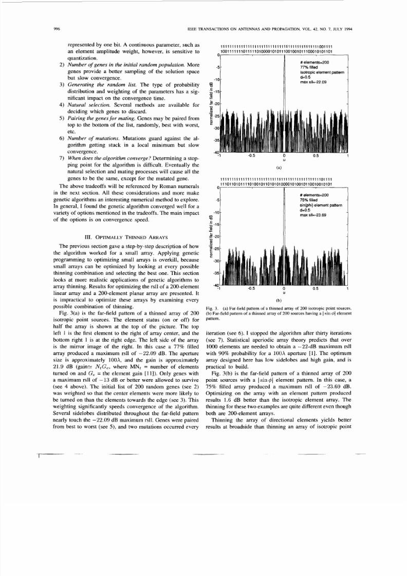
Fig. 4. Far-field pattem in Fig. 3(b) scanned to 120'.

sources of the same size. However, steering the beam away

from broadside causes a significant degradation in the maxi-mum rsll for the array of directional elements.Fig. 4 shows the

antenna pattem in Fig. 3(b) steered to 120'. The maximum rsll

deteriorates to -18.8 dB. The thinned array of isotropic point

sources suffers no sidelobe degradation when the main beam

is steered. Sidelobe degradation for the array of directional

elements may be prevented by optimizing the pattern over the

range of steering angles of the array. For instance, assume

the 200-element array of directional elements steers its beam

between 60' and 120'. The function to be minimized now

retums the maximum rsll over the range of steering angles.

Excellent results are obtained by evaluating the function at

only 120'. The maximum steering angle is the point of

maximum attenuation of the main beam by the element pattern.

Thus, the maximum rsll of all the other steering angles is lower

than at 120'. Fig. 5(a) is the far-field pattern of the 78% filled

200-element array of directional sources at broadside, and

Fig. 5(b) is the pattern when steered to 120'. The maximum

rsll over the scan limits is -22.22 dB. This maximum rsll

is almost the same as that obtained for the array of isotropic

point sources but is less than that obtained in Fig. 3(b).

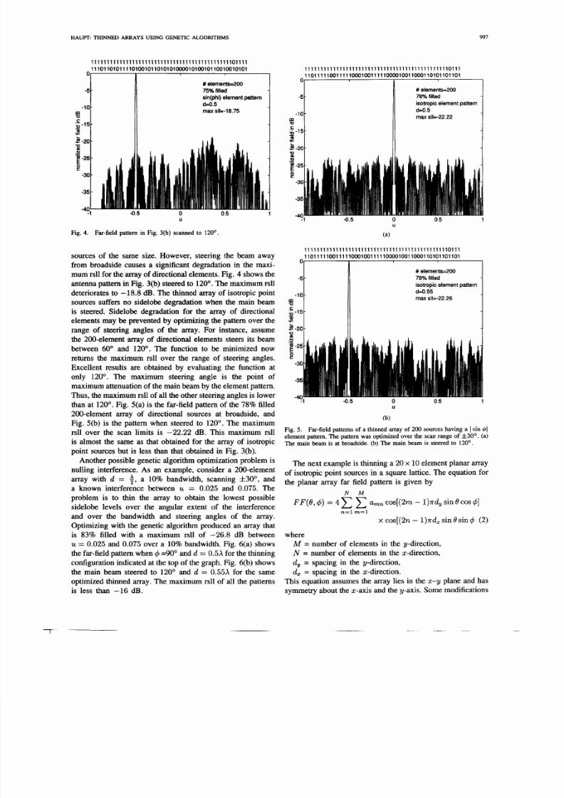
Another possible genetic algorithm optimization problem is

nulling interference. As an example, consider a 200-element

array with d = 4 , a 10% bandwidth, scanning f30', and

a known interference between U = 0.025 and 0.075. The

problem is to thin the array to obtain the lowest possible

sidelobe levels over the angular extent of the interference

and over the bandwidth and steering angles of the array.

Optimizing with the genetic algorithm produced an array that

is 83% filled with a maximum rsll of -26.8 dB betweenU =0.025 and 0.075 over a 10% bandwidth. Fig. 6(a) shows

the far-field pattern when $=90° and d =0.5X for the thinning

configuration indicated at the top of the graph. Fig. 6(b) shows

the main beam steered to 120' and d = 0.55X for the same

optimized thinned array. The maximum rsll of all the patterns

is less than -16 dB.

11111111111111111111111111111111111111111111110111

110111110011111o0o10011111000010011000110101101101

o1I

-5 c

mU

1 - 2 0n

#elements=200

78%filled

isotropic element pattem

max s lb22 .22

d i 0 .5

11111111111111111111111111111111111111111111110111

110111110011111000100111110w010011000110101101101O[ 1

#elements=200

78%filled


max sll=-22.26d=0.55

U

(b)

Fig. 5. Far-field pattems of a thinned array of 200 sources having a I sin 41

element pattem. The pattem was optimized over the scan range of f30'. (a)The main beam is at broadside. (b) The main beam is steered to 120'.

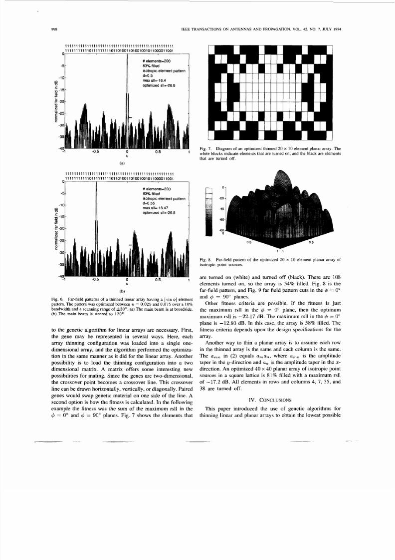
The next example is thinning a 20 x 10 element planar array

of isotropic point sources in a square lattice. The equation for

the planar array far field pattern is given by

N M

FF (B , $ )=4 umncos[(2m - )7rd, sin O cos $1n=l m = l

x cos[(2n- )7rd, sin Osin$ (2)

whereM =number of elements in the y-direction,

N =number of elements in the z-direction,

d , =spacing in the y-direction,

d , = spacing in the z-direction.

This equation assumes the array lies in the E-y plane and has

symmetry about the z-axis and the y-axis. Some modifications



99 8 I€€€ TR

-5

-10-mU

11111111111111111111111111111111111111111111111111

111111111110111111111011010011010010010110000110010

I 1

-

-10-

8c

-15--m._+2 -7n-

-1 5

3 20

#elements=200

83% filled


max sl l=- l6.4

optimized sll=-26.8

d=0.5

-0.5 0U

(a)

0.5 1

11111111111111111111111111111111111111111111111111

11 111111111011111 111101 10100110100100101100001 001

-51

#elements=20083% filled


d=0.55

ma x sll=-l6.47

optimized sll=-26.8

-0.5 0 0.5 1

U

(b)

Fig. 6. Far-field pattems of a thinned linear array having a I sin @ I elementpattem. The pattem was optimized between U =0.025 and 0.0 75 over a 10%

bandwidth and a scanning range of f30'. (a) The main beam is at broadside.(b) The main beam is steered to 120O.

to the genetic algorithm for linear arrays are necessary. First,

the gene may be represented in several ways. Here, each

array thinning configuration was loaded into a single one-

dimensional array, and the algorithm performed the optimiza-

tion in the same manner as it did for the linear array. Another

possibility is to load the thinning configuration into a two

dimensional matrix. A matrix offers some interesting new

possibilities for mating. Since the genes are two-dimensional,

the crossover point becomes a crossover line. This crossover

line can be drawn horizontally, vertically, or diagonally. Paired

genes would swap genetic material on one side of the line. A

second option is how the fitness is calculated. In the following

example the fitness was the sum of the maximum rsll in the

4 = 0" and 4 =90" planes. Fig. 7 shows the elements that

ANSACTIONS ON ANTENNAS AND PROPAGATION, VOL. 42, NO. I, ULY 1994

Fig. 7. Diagram of an optimized thinned 20 x 10 element planar array. Thewhite blocks indicate elements that are turned on, and the black are elementsthat are tumed off.

1 1

Fig. 8.isotropic point sources.

Far-field pattem of the optimized 20 x 10 element planar array of

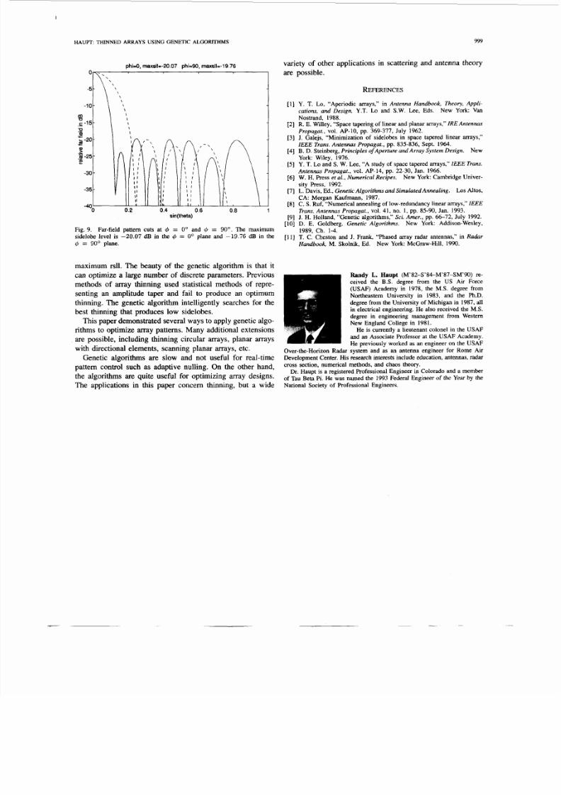
are turned on (white) and turned off (black). There are 108

elements turned on, so the array is 54% filled. Fig. 8 is thefar-field pattern, and Fig. 9 far field pattem cuts in the 4=0"

and 4 = 90" planes.

Other fitness criteria are possible. If the fitness is just

the maximum rsll in the 4 = 0" plane, then the optimum

maximum rsll is -22.17 dB. The maximum rsll in the 4 =0"

plane is -12.93 dB. In this case, the array is 58% filled. The

fitness criteria depends upon the design specifications for the

array.

Another way to thin a planar array is to assume each row

in the thinned array is the same and each column is the same.

The a,, in ( 2 ) equals a,a,, where a,,, is the amplitude

taper in the y-direction and a , is the amplitude taper in the 5 -

direction. An optimized 40 x 40 planar array of isotropic point

sources in a square lattice is 81% filled with a maximum rsll

of -17.2 dB. All elements in rows and columns 4, 7, 35, and

38 are turned off.

IV . CONCLUSIONS

This paper introduced the use of genetic algorithms for

thinning linear and planar arrays to obtain the lowest possible



I

HAUFT THINNED ARRAYS USING GENETIC ALGORITHMS

phi=O, max sll --20.07 phi-90, maxsll =-19.76

0 -.\

sin(theta)

Fig. 9. Far-field pattem cuts at 4 = 0 and 4 = 90”. The maximumsidelobe level is -20.07 dB in the 4 =0 plane and -19.76 dB in the4 =90’ plane.

maximum rsll. The beautyof

the genetic algorithm is that itcan optimize a large number of discrete parameters. Previous

methods of array thinning used statistical methods of repre-

senting an amplitude taper and fail to produce an optimum

thinning. The genetic algorithmintelligently searches for the

best thinning that produces low sidelobes.

This paper demonstrated several ways to apply genetic algo-

rithms to optimize array patterns. Many additional extensions

are possible, including thinning circular arrays, planar arrays

with directional elements, scanning planar arrays, etc.

Genetic algorithms are slow and not useful for real-time

pattern control such as adaptive nulling. On the other hand,

the algorithms are quite useful for optimizing array designs.

The applications in this paper concern thinning, but a wide

999

variety of other applications in scattering and antenna theory

are possible.

REFERENCES

Y. T. Lo, “Aperiodic arrays,” in Antenna Handbook, Theo ry, Appli-cations, and Design, Y.T. Lo and S.W. Lee, Eds. New York VanNostrand, 1988.R. E. Willey, “Space tapering of linear and planar arrays,”IRE Antennas

Propagat.,vol. AP-10, pp. 369-377, July 1962.J. Galejs , “Minimization of sidelobes in space tapered linear arrays,”

IEEE Trans. Antennas Propag at., pp. 835-836, Sept. 1964.B. D. Steinberg, Principles of Aperture and Array System Design. NewYork Wiley, 1976.Y. T. Lo and S. W. Lee, “A study of space tapered arrays,’’ZEEE Trans.Antennas Propagat., vol. AP-14, pp. 22-30, Jan. 1966.W . H. Press et al ., Numerical Recipes. New York: Cambridge Univer-sity Press, 1992.L. Davis, Ed., Generic Algorithms and Simulated Annealing. LosAltos,CA: Morgan Kaufmann, 1987.C. S . Ruf, “Numerical annealing of low-redundancy linear arrays,”ZEEE

Trans. Antennas Pro pagat., vol. 41, no. 1, pp. 85-90, Jan. 1993.J. H. Holland, ”Genetic algorithms,” Sci. Amer., pp. 66-72, July 1992.D. E. Goldberg. Genetic Algorithms. New York Addison-Wesley,

T. C. Cheston and J. Frank, “Phased array radar antennas,” in Radar

Handbook. M. Skolnik, Ed.

1989, Ch. 1-4.

New York McGraw-Hill, 1990.

Randy L. Haupt (M’82-S’84-M’87-SM’90) re-ceived the B.S. degree from the US Air Force(USAF) Academy in 1978, the M.S. degree fromNortheastern University in 1983, and the Ph.D.degree from the University of Michigan in 1987, allin electrical engineering. He also received the M.S.degree in engineering management from WesternNew England College in 1981.

He is currently a lieutenant colonel in the USAFand an Associate Professor at the USAF Academy.He previously worked as an engineer on the USAF

Over-the-Horizon Radar system and as an antenna engineer for Rome AirDevelopment Center. His research interests include education, antennas, radarcross section, numerical methods, and chaos theory.

Dr. Haupt is a registered Professional Engineer in Colorado and a memberof Tau Beta Pi. He was named the 1993 Federal Engineer of the Year by theNational Society of Professional Engineers.

thinned arrays using genetic algorithms

Documents