thickening of mature fine oil sands tailings
TRANSCRIPT
Western University Western University
Scholarship@Western Scholarship@Western
Electronic Thesis and Dissertation Repository
11-25-2014 12:00 AM
Thickening of Mature Fine Oil Sands Tailings Thickening of Mature Fine Oil Sands Tailings
Shriful Islam, The University of Western Ontario
Supervisor: Julie Q Shang, The University of Western Ontario
A thesis submitted in partial fulfillment of the requirements for the Master of Engineering
Science degree in Civil and Environmental Engineering
© Shriful Islam 2014
Follow this and additional works at: https://ir.lib.uwo.ca/etd
Part of the Civil and Environmental Engineering Commons
Recommended Citation Recommended Citation Islam, Shriful, "Thickening of Mature Fine Oil Sands Tailings" (2014). Electronic Thesis and Dissertation Repository. 2566. https://ir.lib.uwo.ca/etd/2566
This Dissertation/Thesis is brought to you for free and open access by Scholarship@Western. It has been accepted for inclusion in Electronic Thesis and Dissertation Repository by an authorized administrator of Scholarship@Western. For more information, please contact [email protected].
THICKENING OF MATURE FINE OIL SANDS TAILINGS
(Thesis format: Monograph)
by
Shriful Islam
Graduate Program in Civil and Environmental Engineering
A thesis submitted in partial fulfillment of the requirements for the degree of
Master of Engineering Science
The School of Graduate and Postdoctoral Studies The University of Western Ontario
London, Ontario, Canada
© Shriful Islam 2015

ii
ABSTRACT
The mature fine oil sands tailings (MFT) remain suspended in tailings disposal pond for
decades because of the low sedimentation/consolidation rate. This study investigates the
application of coagulation and electrokinetics to thicken, i.e., to increase the solid
content of the MFT suspension. At first, the optimal ferric chloride concentration is
identified as 350 mg/l in jar tests, under which the best thickening result is only 6.48%
from an initial of 5% after 4 hours in cylinder coagulation tests. The electrokinetic
thickening under an applied voltage gradient of 219 V/m reaches the final solid content
of 18.75% after 7 hours. The combined coagulation (350 mg/l ferric chloride) and
electrokinetic thickening under a continuous applied voltage gradient (219 V/m) is the
most effective approach, which reaches the final solid content of 23.74%. The
sedimentation theories in the free settling and hindered settling stages are validated
using the experimental results, which is one of the major contributions of this research.
The turbidity of the supernatant ranges between 4.8 NTU and 31 NTU in all treatments.
Two regression models for the electrokinetic and the combined application of
coagulation and electrokinetic tests are developed to relate the final solid content and
the applied voltage gradient. The models and the independent variables are statistically
significant at 95% confidence level based on F-test and t-test results, respectively.
Keywords: electrophoresis, thickening, sedimentation, coagulation, mature fine oil
sands tailings.

iii
DEDICATION
Dedicated to
My Family and The Memory of My Father

iv
ACKNOWLEDGEMENTS
I would like to gratefully thank my supervisor, Dr. Julie Q. Shang, for her invaluable
guidance, assistance, and encouragement throughout my MESc. Her help is not only
important for my study, but also for my life, especially when I was extremely sick.
Working in her group offered me the chance to work on an attractive area of research.
Gratitude and appreciation is expressed to the faculty and staff in the Faculty of
Engineering at Western University, especially to Mr. Tim Stephens, Ms. Melodie
Richards, Ms. Whitney Barrett, Ms. Stephanie Lawrence, and Ms. Cynthia Quintus. The
grateful thanks to Raquibul Alam, Yu Guo, Dr. Saidur Chowdhury, Adnan H Khan,
Shahadat Hossan and other friends for their support, advice and assistance during my
study.
Special thanks to my wife, mother and brothers for supporting and encouraging me
during my study.

v
TABLE OF CONTENTS
CERTIFICATE OF EXAMINATION ................................................. ii
ABSTRACT.......................................................................................... iii
DEDICATION ..................................................................................... iv
ACKNOWLEDGEMENTS ................................................................. v
TABLE OF CONTENTS ..................................................................... vi
LIST OF TABLES ............................................................................... xi
LIST OF FIGURES .............................................................................. xiv
LIST OF SYMBOLS AND ABBREVIATIONS ................................. xix
CHAPTER 1 INTRODUCTION ......................................................................... 1
1.1 General …...................................................................................................... 1
1.2 Research Objectives ……............................................................................. 2
1.3 Thesis Outline ……....................................................................................... 3
1.4 Original Contributions .................................................................................. 4

vi
CHAPTER 2 LITERATURE REVIEW ............................................................. 5
2.1 Introduction ….............................................................................................. 5
2.2 Basic Properties of Oil Sands Tailings ......................................................... 6
2.3 Technologies/Methods for the Treatment of Oil Sands Tailings ................. 8
2.3.1 Physical/Mechanical Process .................................................................. 8
2.3.2 Natural Process ....................................................................................... 9
2.3.3 Chemical Treatment ............................................................................... 10
2.3.4 Mixture/Co-disposal Process .................................................................. 11
2.4 Coagulation ................................................................................................... 11
2.5 Electrokinetics .............................................................................................. 12
2.5.1 Effectiveness of Electrokinetics ............................................................. 13
2.5.2 Effect of Intermittent Current in Electrokinetics .................................... 15
2.6 Theory of Sedimentation/Thickening ........................................................... 15
2.7 Case Study involving Combined Effect of Electrokinetics and Coagulation
....................................................................................................................... 20
2.8 Summary ....................................................................................................... 21
vii
CHAPTER 3 COAGULATION AND ELECTROKINETIC THICKENING
TESTS ON MATURE FINE OIL SANDS TAILINGS ..................................... 23
3.1 Introduction ….............................................................................................. 23
3.2 Properties of Mature Fine Oil Sands Tailings .............................................. 24
3.3 Preparation of MFT Suspensions ................................................................. 26
3.4 Jar Tests for Selection of Coagulant and Optimum Dosage ......................... 27
3.4.1 Experimental Set-up and Procedure ....................................................... 27
3.4.2 Results and Discussion ........................................................................... 28
3.5 Cylinder Coagulation Tests .......................................................................... 30
3.5.1 Experimental Procedure ......................................................................... 30
3.5.2 Results and Discussion ........................................................................... 30
3.5.2.1 Effect of Coagulant Dose ................................................................. 30
3.5.2.2 Effect of pH ...................................................................................... 33
3.6 Electrokinetic Thickening Tests ................................................................... 35
3.6.1 Experimental Set-up ............................................................................... 35
3.6.2 Testing Procedure ................................................................................... 36
3.6.3 Results and Discussion ........................................................................... 37
3.6.3.1 Effect of Initial Solid Content and Applied Voltage Gradient ......... 37
3.6.3.2 Validation of Electrokinetic Sedimentation Theory ......................... 39
3.6.3.3 Power Consumption ......................................................................... 41

viii
3.6.3.4 Zeta Potential of Particles, Water pH, Temperature, and Turbidity
after Electrokinetic Thickening ........................................................ 43
3.6.3.5 Water pH Effect on Final Solid Content .......................................... 44
3.7 Summary ....................................................................................................... 45
CHAPTER 4 COMBINED APPLICATION OF COAGULATION AND
ELECTROKINETIC THICKENING AND OPTIMIZATION OF
RESULTS BY ANOVA ........................................................................................ 79
4.1 Introduction ….............................................................................................. 79
4.2 Combined Application of Coagulation and Electrokinetic Thickening ........ 80
4.2.1 Testing Procedure ................................................................................... 80
4.2.2 Results and Discussion ........................................................................... 81
4.2.2.1 Effect of Applied Voltage Gradient .................................................. 81
4.2.2.2 Power consumption .......................................................................... 83
4.2.2.3 Zeta Potential of Particles and Turbidity of Supernatant after
Combined Tests ................................................................................ 84
4.3 Application of Intermittent Voltage Gradient Combined with Coagulant ... 85
4.3.1 Testing Procedure ................................................................................... 85
4.3.2 Results and Discussion ........................................................................... 86
4.4 Comparison of Thickening Effect by Coagulation, Electrokinetics and
Combined Tests ............................................................................................ 88
ix
4.5 Response Surface Methodology for Regression Model Development ......... 89
4.5.1 Development of Regression Model for Electrokinetic Thickening ........ 90
4.5.2 Development of Regression Model for Combined Coagulation and
Electrokinetic Thickening ....................................................................... 92
4.6 Summary ....................................................................................................... 93
CHAPTER 5 CONCLUSIONS AND RECOMMENDATIONS ...................... 113
5.1 Summary …................................................................................................... 113
5.2 Conclusions ………….................................................................................. 114
5.3 Recommendations for Future Research Work ……...................................... 116
BIBLIOGRAPHY.................................................................................................. 118
APPENDIX............................................................................................................. 125
CURRICULUM VITAE........................................................................................ 126
x
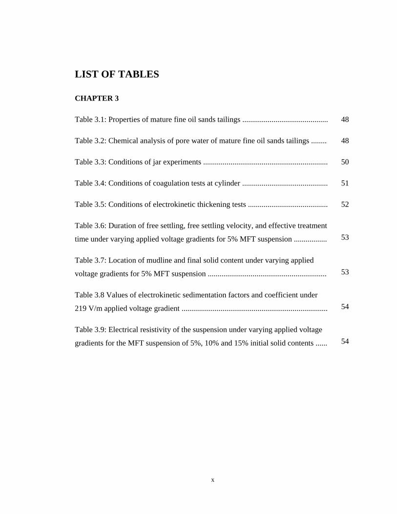
LIST OF TABLES
CHAPTER 3
Table 3.1: Properties of mature fine oil sands tailings ............................................ 48
Table 3.2: Chemical analysis of pore water of mature fine oil sands tailings ........ 48
Table 3.3: Conditions of jar experiments ................................................................ 50
Table 3.4: Conditions of coagulation tests at cylinder ............................................ 51
Table 3.5: Conditions of electrokinetic thickening tests ......................................... 52
Table 3.6: Duration of free settling, free settling velocity, and effective treatment
time under varying applied voltage gradients for 5% MFT suspension ................. 53
Table 3.7: Location of mudline and final solid content under varying applied
voltage gradients for 5% MFT suspension ............................................................. 53
Table 3.8 Values of electrokinetic sedimentation factors and coefficient under
219 V/m applied voltage gradient ........................................................................... 54
Table 3.9: Electrical resistivity of the suspension under varying applied voltage
gradients for the MFT suspension of 5%, 10% and 15% initial solid contents ...... 54

xi
CHAPTER 4
Table 4.1: Conditions of combined coagulation and electrokinetic thickening
tests .......................................................................................................................... 96
Table 4.2: Duration of free settling, free settling velocity and effective treatment
time under combined electrokinetics and coagulation tests for MFT suspension .. 97
Table 4.3: Electrical resistivity of the MFT suspension under varying applied
voltage gradient combined with ferric chloride ...................................................... 97
Table 4.4: Duration of free settling, free settling velocity and effective treatment
time under combined applied voltage gradient and 350 mg/l ferric chloride for
MFT suspension ...................................................................................................... 98
Table 4.5: Comparison of thickening results by coagulation, electrokinetics and
their combined application ...................................................................................... 98
Table 4.6: Factors and levels used in the full three level factorial designs in
electrokinetic thickening ......................................................................................... 99
Table 4.7: Analysis of variance for the final solid content in electrokinetic
thickening ................................................................................................................ 99
Table 4.8: Analysis of variance for the increase in solid content in electrokinetic
thickening ................................................................................................................ 99
Table 4.9: Regression coefficients of full polynomial model for the final solid
content (in coded units) ........................................................................................... 100
Table 4.10: Regression coefficients of full polynomial model for the increase in
solid content (in coded units) .................................................................................. 100
Table 4.11: Factors and levels used in the full three level factorial designs in
combined coagulation and electrokinetic thickening .............................................. 100

xii
Table 4.12: Final solid content of 5% MFT at varying operational condition ........ 101
Table 4.13: Analysis of variance for the final solid content in combined tests ...... 101
Table 4.14: Regression coefficients of full polynomial model for the final solid
content in combined coagulation and electrokinetic thickening ............................. 101
xiii
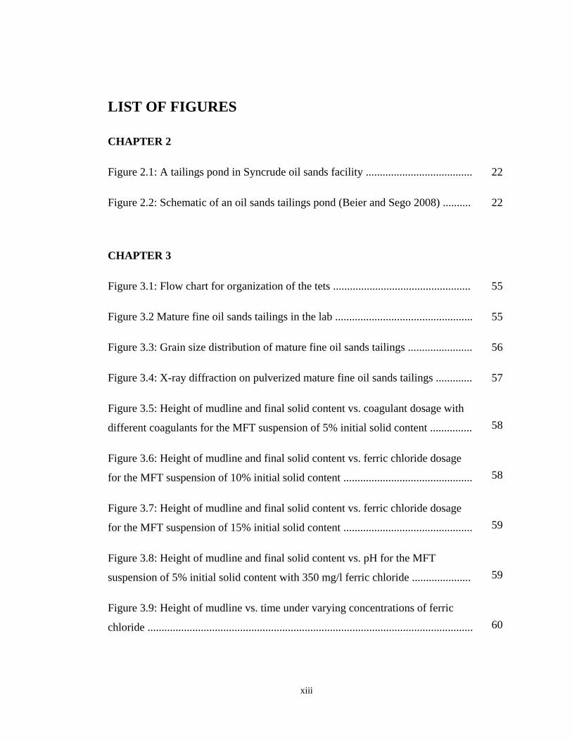
LIST OF FIGURES
CHAPTER 2
Figure 2.1: A tailings pond in Syncrude oil sands facility ...................................... 22
Figure 2.2: Schematic of an oil sands tailings pond (Beier and Sego 2008) .......... 22
CHAPTER 3
Figure 3.1: Flow chart for organization of the tets ................................................. 55
Figure 3.2 Mature fine oil sands tailings in the lab ................................................. 55
Figure 3.3: Grain size distribution of mature fine oil sands tailings ....................... 56
Figure 3.4: X-ray diffraction on pulverized mature fine oil sands tailings ............. 57
Figure 3.5: Height of mudline and final solid content vs. coagulant dosage with
different coagulants for the MFT suspension of 5% initial solid content ............... 58
Figure 3.6: Height of mudline and final solid content vs. ferric chloride dosage
for the MFT suspension of 10% initial solid content .............................................. 58
Figure 3.7: Height of mudline and final solid content vs. ferric chloride dosage
for the MFT suspension of 15% initial solid content .............................................. 59
Figure 3.8: Height of mudline and final solid content vs. pH for the MFT
suspension of 5% initial solid content with 350 mg/l ferric chloride ..................... 59
Figure 3.9: Height of mudline vs. time under varying concentrations of ferric
chloride .................................................................................................................... 60

xiv
Figure 3.10: Settling velocity vs. time under varying concentrations of ferric
chloride .................................................................................................................... 61
Figure 3.11: log(vh/vf) vs. log(n) for the MFT suspension of 5% initial solid
content ..................................................................................................................... 62
Figure 3.12: Final solid content and increase in solid content vs. ferric chloride
dosage ...................................................................................................................... 62
Figure 3.13: Turbidity of supernatant at the top of cylinder for different ferric
chloride dosage ....................................................................................................... 63
Figure 3.14: Total solids of supernatant at the top of cylinder for different ferric
chloride dosage ....................................................................................................... 63
Figure 3.15: Electric conductivity and zeta potential vs. varying dosage of ferric
chloride .................................................................................................................... 64
Figure 3.16: Height of mudline vs. time under varying pH of MFT suspension of
5% initial solid content ........................................................................................... 65
Figure 3.17: Electric conductivity and zeta potential vs. pH of the MFT
suspension of 5% initial solid content ..................................................................... 66
Figure 3.18: Turbidity vs. pH of supernatant at the top of cylinder for 5% MFT .. 66
Figure 3.19: Schematic of Electrokinetic Thickening Column ............................... 67
Figure 3.20: Final location of mudline in an electrokinetic test with control test .. 67
Figure 3.21: Height of mudline vs. time for the MFT suspension of 5% initial
solid content under varying applied voltage gradients ............................................ 68
Figure 3.22: Height of mudline vs. time for the MFT suspension of 10% initial
solid content under varying applied voltage gradients ..............................…...…... 69

xv
Figure 3.23: Height of mudline vs. time for the MFT suspension of 15% initial
solid content under varying applied voltage gradients ............................................ 70
Figure 3.24: Final solid content and increase in solid content vs. applied voltage
gradient for the MFT suspension of 5% initial solid content .................................. 71
Figure 3.25: Final solid content and increase in solid content vs. applied voltage
gradient for the MFT suspension of 10% initial solid content ................................ 71
Figure 3.26: Final solid content and increase in solid content vs. applied voltage
gradient for the MFT suspension of 15% initial solid content ................................ 72
Figure 3.27: Settling velocity vs. time for the MFT suspension of 5% initial solid
content under varying applied voltage gradients .................................................... 73
Figure 3.28: Relationship between free settling velocity and applied voltage
gradient for 5% MFT .............................................................................................. 74
Figure 3.29: log(vh-ek/vf-ek) vs. log(nek) for 5% MFT under 219 V/m applied
voltage gradient ....................................................................................................... 74
Figure 3.30: Effective voltage gradient and voltage efficiency between anode
and cathode vs. applied voltage gradient for 5% MFT ........................................... 75
Figure 3.31: Current density vs. applied voltage gradient for 5% MFT ................. 75
Figure 3.32: Power consumption vs. applied voltage gradient for 5% MFT .......... 76
Figure 3.33: Final zeta potential of particles vs. applied voltage gradient for 5%
MFT ........................................................................................................................ 76
Figure 3.34: Final water pH vs. applied voltage gradient for the MFT suspension
of 5% initial solid content after 7 hours thickening ................................................ 77
Figure 3.35: Final temperature vs. applied voltage gradient for 5% MFT ............. 77

xvi
Figure 3.36: Relationship between turbidity of supernatant and applied voltage
gradient for 5% MFT .............................................................................................. 78
Figure 3.37: Height of mudline and final solid content vs. pH of MFT suspension
at the end of 7 hours thickening tests ...................................................................... 78
CHAPTER 4
Figure 4.1: Height of mudline vs. time under the combined application of applied
voltage gradient and ferric chloride ........................................................................ 102
Figure 4.2: Final solid content and increase in solid content vs. combined applied
voltage gradient and 350 mg/l ferric chloride ......................................................... 103
Figure 4.3: Settling velocity vs. time under the combined applied voltage
gradient and ferric chloride ..................................................................................... 104
Figure 4.4: Effective voltage gradient and voltage efficiency between anode and
cathode vs. applied voltage gradient combined with ferric chloride ...................... 105
Figure 4.5: Current density vs. applied voltage gradient combined with ferric
chloride .................................................................................................................... 105
Figure 4.6: Power consumption vs. applied voltage gradient combined with ferric
chloride .................................................................................................................... 106
Figure 4.7: Final zeta potential of particles vs. applied voltage gradient under the
combined application of electrokinetics and coagulation ....................................... 106
Figure 4.8: Turbidity of supernatant under varying applied voltage gradient
combined with ferric chloride at the end of the tests .............................................. 107
Figure 4.9: Height of mudline vs. time under the combined application of
intermittent applied voltage gradient and ferric chloride ……….…………….….. 108
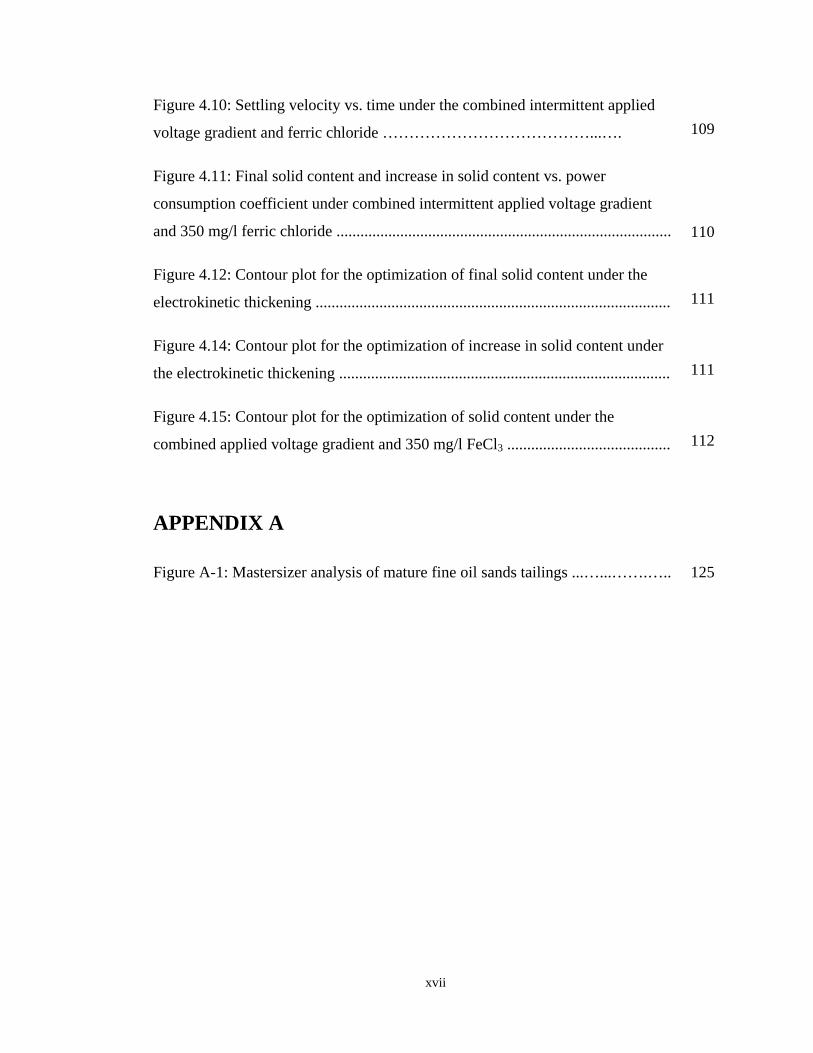
xvii
Figure 4.10: Settling velocity vs. time under the combined intermittent applied
voltage gradient and ferric chloride …………………………………...…. 109
Figure 4.11: Final solid content and increase in solid content vs. power
consumption coefficient under combined intermittent applied voltage gradient
and 350 mg/l ferric chloride .................................................................................... 110
Figure 4.12: Contour plot for the optimization of final solid content under the
electrokinetic thickening ......................................................................................... 111
Figure 4.14: Contour plot for the optimization of increase in solid content under
the electrokinetic thickening ................................................................................... 111
Figure 4.15: Contour plot for the optimization of solid content under the
combined applied voltage gradient and 350 mg/l FeCl3 ......................................... 112
APPENDIX A
Figure A-1: Mastersizer analysis of mature fine oil sands tailings ...…...…….….. 125
xviii
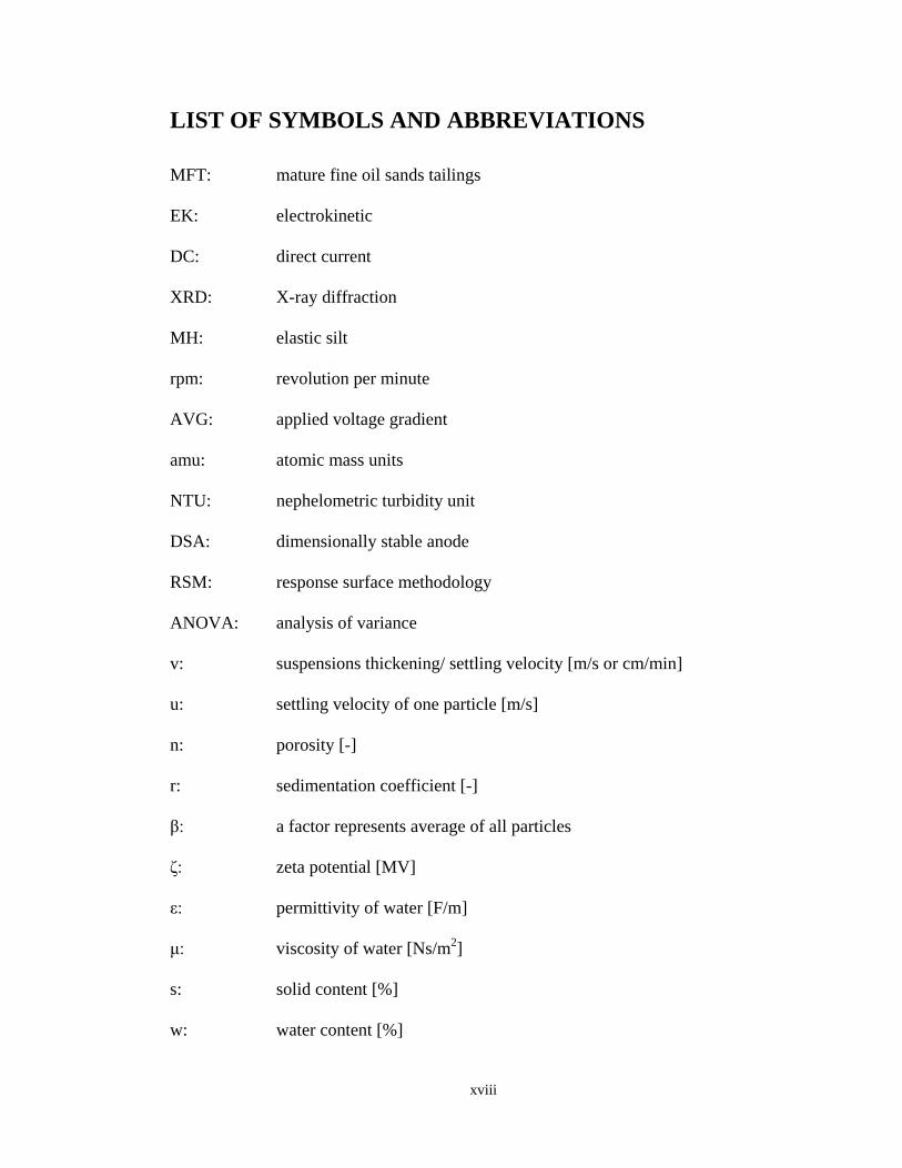
LIST OF SYMBOLS AND ABBREVIATIONS
MFT: mature fine oil sands tailings
EK: electrokinetic
DC: direct current
XRD: X-ray diffraction
MH: elastic silt
rpm: revolution per minute
AVG: applied voltage gradient
amu: atomic mass units
NTU: nephelometric turbidity unit
DSA: dimensionally stable anode
RSM: response surface methodology
ANOVA: analysis of variance
v: suspensions thickening/ settling velocity [m/s or cm/min]
u: settling velocity of one particle [m/s]
n: porosity [-]
r: sedimentation coefficient [-]
β: a factor represents average of all particles
ζ: zeta potential [MV]
ε: permittivity of water [F/m]
μ: viscosity of water [Ns/m2]
s: solid content [%]
w: water content [%]
xix
Gs: specific gravity [-]
LL: liquid limit [%]
PL: plastic limit [%]
PI: plasticity index [%]
EC: electrical conductivity [mS/cm]
H: height of mudline [cm]
t: time [min]
U: voltage [V]
E: voltage gradient [V/m]
I: electric current [A]
A: cross-section area [m2]
j: current density [A/m2]
ρ: electrical resistivity [Ω-m]
ρs: density of MFT solids [kg/m3]
ρf: density of MFT fluids [kg/m3]
V: volume of MFT [m3]
P: power consumption [W/m3]
T: temperature [0C]
χ: power consumption coefficient [%]
α1/α2/α3: coefficient of regression models
y: response variable in regression model
x1/x2/x3: independent variables in regression model

1
CHAPTER 1 INTRODUCTION
1.1 General
Oil sands tailings are the end by-products of oil sands processing, which are discharged
as slurry containing low percentage of solids. Mine tailings have potential impacts to the
environment such as water pollution, solid waste, land use and reclamation, and air
pollution. After releasing to a disposal pond, the coarse solids in tailings settle quickly,
and the water rises to the top. However fine solids, namely the mature fine oil sands
tailings (MFT), contain clay materials and fine sands, remain suspended in water for long
time. It takes a few years for some MFT to reach solids contents of 30-35% (Beier and
Sego 2008, Scott 1985) by gravity alone. The oil sand industries use huge amount of
water to extract bitumen from oil sands. The slow settling of fine particles and large
portion of standing water in tailings are challenging to the management of containment
facilities for a long time beyond the mine closure. Active researches are undertaking in an
effort to increase the solid contents of mature fine oil sands tailings in the underflow and
to accelerate water recycling through the overflow of the system, which is known as
thickening (Concha and Burger 2003).
Thickening is a preliminary method to produce high solid slurries (Gladman et al. 2006),
which will ease further dewatering. The operation of a sedimentation unit is categorized
as thickening and clarification (Jewell and Fourie 2006). The aim of clarification is to
produce an overflow of water with few or no solid particles present, while the objective
of thickening is to generate an underflow with high solids concentration. Thickening by

2
gravity depends on the difference of densities between the solid and liquid phases. It
becomes slower with time when the solid concentration of the slurry increases. Moreover,
the self-weight consolidation is very slow for the fine tailings produced in the oil sands
industries. So the mature fine oil sands mine tailings require additional treatment (such as
coagulant, flocculants, filtration, vacuum, electrokinetics, etc.) to enhance thickening
process. The filtration technology is not favorable due to presence of high percentage of
fines in the tailings (Xu et al. 2008). The polymer flocculants may create environmental
problem. The applicability of vacuum technology in huge oil sands fields is a concern. So
in this study, coagulation, electrokinetics, and combined coagulation and electrokinetics
are selected to thicken the MFT suspension to increase the solid concentration of the
underflow. Coagulation-electrokinetic combined treatment is based on making larger
flocs of particle in the suspensions with coagulants and then generating movement of
solids by a direct current (DC). This study is limited in laboratory scale and so some real
field factors such as solid content variation, effect of wind and temperature variation,
flow conditions are missed out.
1.2 Research Objectives
The overall objective of this research is to thicken the mature fine oil sands tailings by
combined chemical coagulants and electrokinetics. The specific objectives are:
• Measure the properties of mature fine oil sands mine tailings;
3
• Optimize coagulant doses in jars and study the coagulation effect in cylinders in
thickening the suspension of MFT;
• Optimize the voltage gradient in achieving highest the solid content of the
sediment;
• Attain the possible maximum solid content of the sediment in the combined
application of coagulant and electric current;
• Study characteristics of water and solids after treatment;
• Develop regression models to determine the final solid content of MFT.
1.3 Thesis Outline
The thesis consists of five chapters. Chapter 1 contains an introduction of the thesis
including the research objectives, outline and original contributions.
Chapter 2 presents a literature review related to the properties of mature fine oil sands
tailings, treatment technologies of oil sands tailings, and principles and applications of
electrokinetics and chemical coagulation.
Chapter 3 is comprised of geotechnical and chemical properties of mature fine oil sands
tailings used in this study, optimization of coagulant and coagulant doses, testing
procedures and results of coagulation and electrokinetic thickening.
Chapter 4 presents the operation, results and discussion of combined coagulant and
electrokinetic thickening tests, including the development of regression models for

4
electrokinetic thickening, and combined application of coagulation and electrokinetic
thickening.
Chapter 5 includes the summery of this study as well as conclusions and
recommendations for further research.
1.4 Original Contributions
The original contributions of this study are:
• Original results of experiments on electrokinetic thickening of mature fine oil
sands tailings;
• The equations of settling velocity in the free settling and hindered settling stages
are validated using the experimental data;
• Original results of experiments on combined coagulation and electrokinetic
thickening;
• Regression models for the final solid content generated by the electrokinetic
thickening as well as by the combined coagulation and electrokinetic thickening.
5
CHAPTER 2 LITERATURE REVIEW
2.1 Introduction
A review for common properties of oil sands tailings is presented and discussed in this
chapter, including principles and applications of coagulation and electrokinetics. A case
relevant to the present research is also assessed in brief.
The mature fine oil sands tailings have solids mostly less than 44 µm in sizes (called
fines in oil sands industries). Without treatment the full consolidation of MFT may take
few decades because of the low settlement or consolidation rate. It is crucial to increase
the rate of thickening process for tailings disposal. Chemical coagulation and
electrokinetics can be applied to accelerate the rate of thickening. Coagulants have been
used in settling of river sediment (Buckland et al. 2000), waste water treatment
(Genovese and Gonzalez 1998) and treatment of collected water from oil sands
processing system (Pourrezaei and El-Din 2008). Research and field applications have
been carried out using electrokinetics to settle, dewater and consolidate soft clays and
mine tailings (Sprute and Kelsh 1980, Lockhart and Stickland 1984, Mohamedelhassan
2008, Guo and Shang 2014). Polymers are also used to flocculate the oil sands tailings to
enhance the separation (Wang et al. 2010). However, the polymer flocculants have
unpredictable performance due to tailings variability and may generate detrimental
effects on recycle water quality (BGC 2010). Moreover, some polymer flocculants are
temperature sensitive.

6
In open pit mining, the oil sands industries use hot water for extraction bitumen from oil
sands and the extracted tailings (by product) stored in the tailings pond. About 750
million cubic metres of MFT was placed in tailings ponds as of 2008 (BGC 2010). The
inventory of fine tailings is predicted to reach one billion cubic metres in 2014 and two
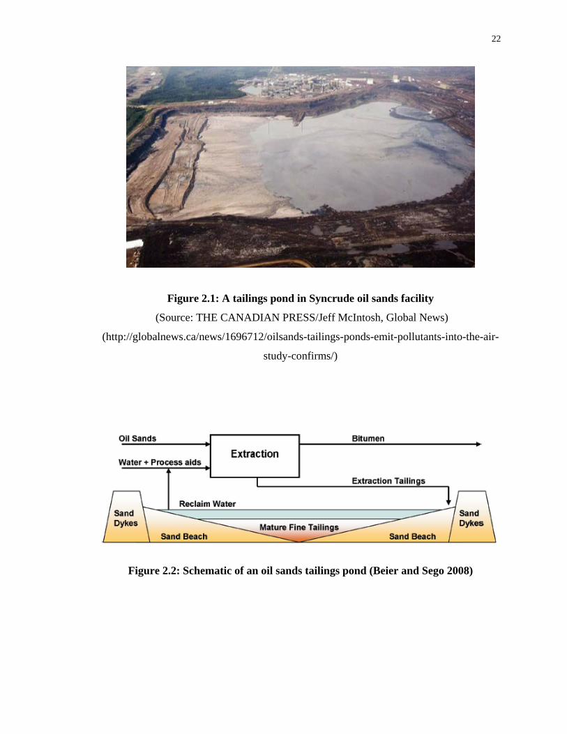
billion in 2034 (Houlihan and Haneef 2008). A photograph of tailings pond in Syncrude
oil sands facility is shown in Fig. 2.1. Eight tailings ponds in Suncor cover a total area of
3,154 hectares and depths are mostly 45.7 metres (Suncor 2010). At the end of 2009,
tailings ponds cover more than 130 square kilometers in the oil sands region
(Government of Alberta 2010) and it is forecasted that it will reach about 250 square
kilometers by 2020. Many mine companies dispose their waste repeatedly on highly
constraint areas due to their abundance of deposits. They need to compete for limited
space for tailings ponds, overburden dumps, lift dewatering area, and other disposal
facilities. So it is crucial to reduce the volume of oil sands tailings and environmental
concern for the sustainable development of oil sands industries and economy. The
electrophoresis can be applied to increase the solid content of the slurry when initial solid
content of MFT is low and then further dewatering to consolidate the thickened MFT.
2.2 Basic Properties of Oil Sands Tailings
Oil sands tailings are the byproduct from the extraction of bitumen from oil sands ore.
Most of the oil sands industries are situated in northern Alberta where the oil sands
deposits contain approximately 1.6 trillion barrels of bitumen. According to Kasperski

7
(1992) oil sands tailings compositions vary considerably; however the following
discussion represents an overview about it.
Athabasca oil sands, the largest oil sands reserve, are composed of 0~17 wt% bitumen,
84~86 wt% minerals (such as quartz, silts, clay) and 3~6 wt% water. Kaolinite (40~70
wt%), illite (28~45 wt%) and trace montmorillonite are the major clay minerals
(Chalaturnyk et al. 2002). The oil sands tailings in northern Alberta contain water
(58~62%), solids (sand and clays, 37%) and a small amount of uncovered bitumen
(1~5%) (Cabrera et al. 2009). It is reported that the MFT has an average solid content of
about 33%, average void ratio of 5, hydraulic conductivity from 1×10⁻⁶ to 1×10⁻⁹ m/s,
liquid and plastic limits ranging from 40% to 75% and 10% to 20%, respectively, and the
shear strength less than 1 kPa. The average particle size of MFT ranges between 5 μm
and 10 μm (FTFC 1995).
The majority of clay minerals in the tailings come from the clay shale, discontinuous
seams and layers since these are broken up during the mining extraction process (Scott et
al. 2008). The fine tailings of Syncrude’s caustic extraction process consists of 94%
fines, 76% clay minerals (55% kaolinite, 20% illite, and 1% mixed layers) and 24% rock-
forming minerals (19% quartz, 3% siderite, 1% plagioclase, and 1% K-feldspar). The
water pH is 8.2. The water of fine oil sands tailings mainly contains five cations and four
anions which are: Na+ (258 mg/l), NH4+ (8.8 mg/l), K+ (7.8 mg/l), Ca2+ (5.9 mg/l), Mg2+
(4.1 mg/l), HCO3– (846 mg/l), Cl– (94 mg/l), F– (8.2 mg/l), and SO4
2– (4.8 mg/l) (Scot et
al. 2008). The coarse grained particles in the tailings settle faster than the fines and settle
quickly at the edge of the tailings pond. The fines accumulate at the center of the pond, as
shown in Fig. 2.2 and remain suspended for more than a decade without any treatment.
8
2.3 Technologies/Methods for the Treatment of Oil Sands
Tailings
The major technologies that have been implemented or have the potential of application
for the treatment of oil sands tailings are as follows (BGC 2010):
Physical/Mechanical Process
Natural Process
Chemical Treatment
Mixture/Co-disposal
2.3.1 Physical/Mechanical Process
Filtration is one of the conventional methods used in industries to separate solid-liquid
from mixtures. In the 1990s, Alberta’s oil sands industry conducted pilot-scale tests on
different bitumen extraction process (FTFC 1995). These tests were failed because coarse
particles settled quickly and made a bulky permeable filter cake; however, the fines settle
slowly onto the surface of this cake and blind it, and shutting off filtration. Xu et al.
(2008) carried out laboratory-scale experiments and found that filtration is not realistic to
filter the original tailings with more than 4% fines without using flocculant, while the
mean fines content of the whole tailings stream is about 18%.

9
Solid-liquid separation by centrifuge applies up to thousands of times the force of gravity
to extract fluid, which can increase the solid content to about 60%. Mikula et al. (2009)
developed centrifuge technology at bench scale at Canada Centre for Mineral and Energy
Technology (CANMET) on Athabasca oil sands fluid fine tailings. More research work is
needed to evaluate this technology in field application due to their high capital and
operating cost, and some knowledge gaps.
Electrical treatment applies a direct current (DC) to MFT through electrodes. The
charged clay particles moves to anode (soil in water system), resulting in accelerated
sedimentation and in some cases water flows from an anode to cathode in porous media
(water in a soil system), resulting in dewatering and consolidation of MFT induced by a
DC electric field. A detailed review of electrokinetics is presented in Section 2.5.
2.3.2 Natural Process
The freeze-thaw technology involves the MFT freezing first, then the frozen mass is
permitted to thaw in the following summer (BGC 2010). A significant amount of water is
released when 5 cm to 15 cm thin layers of MFT are subjected to freeze-thaw cycles
(Dawson and Sego 1993). At the end of the tests, the solids content increased from 35%
to 56%. But this process depends on the weather conditions of the region.
Sedimentation and consolidation use the force of gravity to separate the solids from the
tailings stream. This technique has been used for 40 years in oil sands, but despite tens of
10
millions of dollars of research, perceptive of the basics of densification of MFT remains
intangible (BGC 2010).
Dewatering by plant is another method to dewater MFT by selecting suitable plant
species growing on tailings, which can dewater tailings by transpiration through their
leaves and associated root systems (Silva 1999). Silva (1999) shows that appropriate
plant species growing in composite tailings have the ability to take out the water through
evapotranspiration that increase the undrained shear strength and bearing capacity within
the root zone. The plant root system also provides fiber reinforcement and contributes to
the increase in the bearing capacity of the rooted tailings. The main problem in this
technique is high alkalinity and salinity of tailings pore water, which restricts the
establishment of vegetation.
2.3.3 Chemical Treatment
Coagulants and flocculants are widely used in water treatment, which can efficiently
settle the fine particle in tailings. When fine tailings are mixed with these chosen
chemicals, the time of settling can be reduced, and comparatively high solid content can
be attained (Jeeravipoolvarn 2010). The technology is still in applied research and
demonstration level (BGC 2010). The process of coagulation will be reviewed in detail in
the next section of this chapter.
11
2.3.4 Mixture/Co-disposal Process
Composite tailings (CT) process was developed at the University of Alberta (Caughill et
al. 1993), which involves mixing dense extraction tailings (coarse sand) and MFT at 4:1
sand to fine ratio with an amendment (typically gypsum) to create non-segregating slurry.
Syncrude implemented the CT process on a commercial basis in 2000 (Fair 2008). More
works are needed to produce less energy consuming, more environment friendly, and
more qualified CT.
2.4 Coagulation
Coagulation is a common technique in water and wastewater treatment to enhance
sedimentation. Jar test is universally used to assess the optimum dosage for coagulation
in a given medium. Various types of coagulants are used in thickening or dewatering of
mine tailings. Among all Al3+ and Fe+3 salts are most commonly used as coagulants
(Jewell and Fourie 2006) since trivalent ions are more effective than monovalent or
divalent ions as coagulant.
A research was performed by Genovese and Gonzalez (1998) on solids removal from
fisheries wastewaters using coagulants. The tests were executed in batch approach using
1 L flasks. The maximum removal of solid content was 30.5% with 60 mg/l ferric
chloride (FeCl3) as coagulant at pH 5.5. Pourrezaei and El-Din (2008) used alum
(Al2(SO4)3.18H2O) as coagulant to treat oil sands processing water. Ferric chloride has
12
been used as an effective coagulant for the sedimentation of contaminated Welland River
sediment (Buckland et al. 2000).
In this research three common inorganic salts, i.e. ferric chloride, aluminum sulphate and
aluminum chloride, are examined as coagulants to thicken the mature fine oil sands
tailings. These coagulants work well due to the high valence of Fe3+ and Al3+, which are
attracted strongly to the particles of the suspension reducing the thickness of double
layer. At higher coagulant doses (>5mg/l) the coagulant acts by making sweep-floc along
with destabilization. The effectiveness of different coagulants is evaluated at different
coagulant dosage and pH to find the optimal operational conditions to thicken the MFT
suspensions.
2.5 Electrokinetics
Electrokinetics is the movement of ions, water or charged solid particles towards the
electrodes under the influence of an electric field. The US Bureau of Mining carried out
the research on electrokinetic dewatering of tailings from coal preparation and mineral
processing in the 1960s (Stanczyk and Feld 1964). In the 1970s, the CSIRO of Australia
started research on electrokinetic dewatering of tailings (Lockhart 1986). The principle of
electrokinetic sedimentation of clay suspension is discussed by Shang (1997). The
suspended solids are negatively charged in water; hence when they approach to other the
negative charges on the solids causes them to repel. Since the attractive force between the
particles is less than the repulsive force, the suspension remains stable without significant

13
settlement for a long time. When the suspension is subjected to an external electric field,
the negatively charged particles move towards the positively charged anodes. This
phenomenon is known as electrophoresis, which can enhance the sedimentation process.
The mechanism of electrophoresis has been applied to accelerate sedimentation of river
sediments (Buckland et al. 2000) and cohesive soils (Kim et al. 2008).
When a direct current is passing from anode (+Ve) to cathode (−Ve) in water, oxidation
and reduction happens at anode and cathode, respectively. The electrochemical reactions
in anode and cathode release oxygen and hydrogen gas, respectively (Mitchell 1993)
from electrolysis of water which are:
2H2O − 4e−→ O2 + 4H+ (at anode)
4H2O + 4e−→2H2 + 4OH− (at cathode)
The electrophoresis technique will be used by applying DC electric current through the
electrodes to thicken the MFT suspensions.
2.5.1 Effectiveness of Electrokinetics
Researches indicate that electrokinetics is effective in materials containing 30% or more
solids finer than 2 micrometer. The effectiveness of electrokinetics changes with pH
because the electrical charges of colloidal particle are pH dependent. The surface charges
reverse polarity with low pH. The electrokinetic sedimentation of soil-water suspension
has been successful in pH 6-8.5 (Kim et al. 2008) and pH 7.5 (Buckland et al. 2000). The

14
selection of electrode is another important element for the effectiveness of electrokinetic
process. The common problem of using metal electrodes is the high corrosion rate at the
anodes due to decrease in pH, and voltage loss at the electrodes and water interface.
Corrosion of metal (steel mesh) anode has been reported in previous a study as 1.1 kg/dry
tonne of coal washery tailings (Lockhart and Stickland 1984). Different combinations of
anode-cathode (carbon-carbon, carbon-steel, carbon-copper, steel-steel, steel-carbon and
copper-copper) have been tried in marine sediment recovery and found large voltage drop
for carbon-coated electrodes (Mohamedelhassan and Shang 2001). However, Buckland et
al. (2000) used graphite electrode as both anode and cathode in electrokinetic
sedimentation of contaminated Welland River sediment, and found a good result in
voltage efficiency (93-95%) and percentage increase (39-62%) in solid content. More
recently dimensionally stable anode (DSA) mesh (made of titanium coated with iridium
oxide (Ti/IrOx) has been developed, which can serve for a long time compared to other
metals. Stainless steel mesh (type SS316) is found well as cathode material for its
excellent resistance to natural corrosion. Guo and Shang (2014) used Ti/IrOx-SS316
anode-cathode combination in electrokinetic dewatering of oil sands tailings and got
good results in terms of increment in undrained shear strength and reductions in water
content of MFT. In this research Ti/IrOx and SS316 mesh electrodes are selected as
anode and cathode, respectively to thicken the MFT suspensions.

15
2.5.2 Effect of Intermittent Current in Electrokinetics
Current intermittence is a process in which the electric current is applied periodically at
predetermined time interval during the tests. The intermittent voltage (or current) reduces
the power consumption, and possibly enhances the electrokinetic process as reported by
Shang and Lo (1997) and Rabie et al. (1994). The contradictory results are found in
different literature regarding the effectiveness of intermittent voltage to the electrokinetic
processes in soil-water system. The enhanced results were found from the use of
intermittent current on consolidated marine sediment by Shang and Lo (1997), whereas
Buckland et al. (2000) found the best sedimentation effect with continuous electric
current compared with those of intermittent current. The soil and water properties of the
samples might lead to the conflicting results. The effect of intermittent applied voltage
gradient combined with coagulant will be studied to examine the effect of intermittent
voltage on thickening of MFT suspension.
2.6 Theory of Sedimentation/Thickening
The separation of solid particles and liquids by settling under gravity is termed as
sedimentation. Many parameters (particle size and shape, specific gravity, fluid viscosity,
solid concentration, and interaction between particles) can affect the settling velocity
(Svarovsky 1990). The sedimentation velocity of suspensions decreases with the increase
in particles interactions and solid concentrations.

16
The sedimentation velocity of a suspension with low solid concentration can be measured
from Stokes law that follows free settling and can be written as:
( )µρρ
18
2dgu fs −= (2.1)
Where u is the particle settling velocity (m/s), g is the gravitational acceleration (m/s2), ρs
and ρf are the densities of MFT solids and fluid (kg/m3), respectively, d is the diameter of
particle (m), and μ is the viscosity of fluid (N.s/m2).
Kynch (1952) found Stokes law is inadequate for a suspension of high concentration and
developed the Hindered settling theory. According to Kynch’s theory, the sedimentation
velocity decreases as the solid concentration of suspension increases. Jeeravipoolvarn
(2010) studied the oil sands tailings, and showed that the sedimentation followed the
Kynch’s theory with initial solid contents of 10%, 12.5% and 17.5%. Richardson and
Zaki (1954) showed from experimental work that suspension velocity of particles
(spherical shape) depends upon solid concentration and proposed the equation of
suspension velocity which is:
rnuv .= (2.2)
Where v is the suspensions sedimentation velocity, n represents the porosity, and r is the
sedimentation coefficient.
McRoberts and Nixon (1976) showed that the sedimentation velocity decreased with the
increase in initial solid concentration for soil-water mixtures of varying concentration.
However, a transition stage between constant velocity and consolidation was observed for
17
fine-grained soil. This stage is known as hindered settling stage and gave a non-linear
decrease in mudline with time. The hindered settling for the slurry with fine particles are
well established when the porosity of slurry well below unity. Few researchers have
modified the Richardson and Zaki’s sedimentation theory by changing the function of
porosity (Souslby 1997 and Dankers and Winterwerp 2007).
The theory of sedimentation developed by Richardson and Zaki (1954) is applicable for
the suspension of particles size more than 100 μm. Reynolds number is also considered in
many studies which characterizes the flow regime around a settling particle (Camenen
and Bang 2011). In this study the experiment is started when the suspension is stable
initially (without turbulence). A factor (β) is incorporated in the sedimentation equation
of Richardson and Zaki (1954) relating the terminal settling velocity of particles and
sedimentation velocity of the suspension which is due to the effect of flow regime and the
existence of high percentage of fine particles in the slurry. So the Equation 2.2 for free
settling and hindered settling (gravitational) settling stages for fine particles, following
the work of Buckland et al. (2000), can be expressed as:
rnuv ..β= (2.3)
Where β is a factor that relates the particle’s terminal velocity and suspensions thickening
velocity. The sedimentation velocity would constant for an infinitely dilute solution,
indicating the free settling stage and the equation becomes:
uv ff .β= (2.4)

18
Where the subscript f stands for free settling. When the particle interaction increased, the
free settling stage disappears at the critical sedimentation point and changes to hindered
settling stage, and hence, the velocity of the sediment is decreased. The sedimentation
velocity during this stage can be presented as:
rhh nuv ..β= (2.5)
Where the subscript h denotes hindered settling. As the velocity of the suspension
diminished, the sedimentation velocity becomes zero, and the hindered settling is
completed.
The sedimentation coefficient for gravitational settling, r, can be found by combining
Equations 2.4 and 2.5:
nrvv
f
h loglog +=
γ (2.6)
Where
=
f
h
ββ
γ log
Shang (1997) has developed the equations for electrokinetic sedimentation velocity
created by DC electric field with the arrangement of cathode at the top and anode at the
bottom of the electrokinetic column. The equations for free and hindered settling stages
are as follows:
ekekfekf uv .−− = β (2.7)
ekrekekekhekh nuv ..−− = β (2.8)
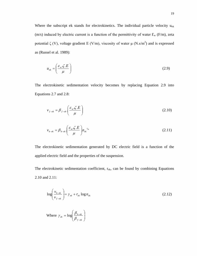
19
Where the subscript ek stands for electrokinetics. The individual particle velocity uek
(m/s) induced by electric current is a function of the permittivity of water Ɛw (F/m), zeta
potential ζ (V), voltage gradient E (V/m), viscosity of water μ (N.s/m2) and is expressed
as (Russel et al. 1989):
=
µζε E
u wek
.. (2.9)
The electrokinetic sedimentation velocity becomes by replacing Equation 2.9 into
Equations 2.7 and 2.8:
= −− µ
ζεβ
Ev w
ekfekf..
. (2.10)
ekrek
wekhekh n
Ev .
...
= −− µ
ζεβ (2.11)
The electrokinetic sedimentation generated by DC electric field is a function of the
applied electric field and the properties of the suspension.
The electrokinetic sedimentation coefficient, rek, can be found by combining Equations
2.10 and 2.11:
ekekekekf
ekh nrvv
loglog +=
−
− γ (2.12)
Where
=
−
−
ekf
ekhek β
βγ log

20
The theories described in this section will be validated using the experimental results in
the next chapter. In the experimental study it will be assumed that there is no turbulence
of suspension in the column.
2.7 Case Study involving Combined Effect of Electrokinetics and
Coagulation
A case on the sedimentation of Welland River sediment using coagulant enhanced
electrokinetics is discussed in this section because of its relevance with the present
research. Buckland et al. (2000) carried out an experimental study on the sedimentation
of contaminated sediment dredged from the Welland River, Ontario, Canada. In the
electrokinetic columns, the anode was placed at the bottom and cathode at the top. The
electrodes (anode and cathode), made of copper, were connected with a DC power
supply. The maximum electric field intensity applied was 150 V/m. The optimum
electrokinetic sedimentation was found from the slurry with the initial solid concentration
of 14.4% and the final solid concentration reached 51%. The maximum decrease of
overall sedimentation time was about 50% compared to the control test. The best result
was found for an electric field intensity of 150 V/m with a voltage efficiency of 91.3%.
From a series of jar tests, 40 mg/l ferric chloride was found to be the most effective
coagulant. The electrokinetic sedimentation was more effective than that of ferric
chloride in terms of increasing the final solid content. The combined action of
electrokinetics and coagulant produced the best sedimentation for the Welland River

21
sediment. The final solid concentration reached 61% from the initial concentration of
14.4% in the combined study. The pH changes due to the application of electrokinetics
were observed at the anode and cathode and were found to be above 6 and below 9.4,
respectively.
2.8 Summary
A review of properties with treatment technologies of oil sands tailings are presented in
this chapter. The effectiveness of coagulation and electrokinetics, and the theory of
electrokinetics and applications are discussed. The materials discussed in literature/case
provide encouraging background for the present study on thickening of mature fine oil
sands tailings. The theory discussed in this chapter will be validated by using the
experimental data found in this research. The coefficients of sedimentation will also be
determined.
22
Figure 2.1: A tailings pond in Syncrude oil sands facility
(Source: THE CANADIAN PRESS/Jeff McIntosh, Global News)
(http://globalnews.ca/news/1696712/oilsands-tailings-ponds-emit-pollutants-into-the-air-
study-confirms/)
Figure 2.2: Schematic of an oil sands tailings pond (Beier and Sego 2008)
23
CHAPTER 3 COAGULATION AND ELECTROKINETIC
THICKENING TESTS ON MATURE FINE OIL SANDS
TAILINGS
3.1 Introduction
The properties of mature fine oil sands tailings (MFT), and results of coagulation and
electrokinetic tests are analyzed and presented in this chapter. Detailed discussion
includes the testing procedures of coagulation and electrokinetic thickening, selection of
coagulants, optimization of coagulant dosage, results, analysis and comparison of
coagulation and electrokinetic thickening tests. Moreover, the theories of sedimentation
velocity are validated using the experimental data.
The characterization of MFT consists of geotechnical properties of tailings (specific
gravity, particle size analysis, Atterberg limits, etc.), X-ray diffraction (XRD) of solids,
and chemical analysis of the pore water. The coagulation tests are carried in jars to find
out the suitable coagulants and optimal dosage among alum (Al2(SO4)3.18H2O),
aluminum chloride (AlCl3) and ferric chloride (FeCl3).
In the 2nd phase of study, coagulation tests are carried on in graduated cylinders to
thicken the MFT suspension. The results are discussed in terms of the mudline (interface
between solids and water) position and final solid content of the thickened tailings. The
suspensions settling velocity and turbidity of the supernatant are measured.
24
The 3rd phase of study involves the electrokinetic thickening tests on the MFT suspension
in the electrokinetic column. The results are monitored with real time in terms of the
mudline position and the final solid contents. The parameters such as the effective
voltage, power consumption, water pH, temperature and turbidity of supernatant are
examined. The theory of electrokinetic sedimentation velocity is validated using the
results of the tests.
The organization of the tests is shown in Fig. 3.1. The jar experiments are designed to
select the suitable coagulant and optimal dosage for the most effective sedimentation.
Then the coagulation tests in the cylinder are carried out to thicken the suspension of
mature fine oil sands tailings. Finally, electrokinetic thickening tests are conducted by
applying a DC electric current.
3.2 Properties of Mature Fine Oil Sands Tailings
The mature fine oil sands tailings used in this research were collected from the disposal
pond in Fort McMurray, Alberta, Canada. Three barrels MFT were provided, courtesy of
Syncrude Canada Ltd. and Imperial Oil Canada. The photograph of mature fine oil sands
tailings in a small tray in the lab is shown in Fig. 3.2. The tailings are dark grey color
with a strong odor and have a natural water content1 of 158%. The specific gravity of
solids is 2.58. The amount of oil and grease in MFT is 1.67 g/l (ASTM D7575). The
organic content of MFT is determined by burning the dried pulverized MFT in muffle
1 Water content (%) = (mass of water / mass of solids)*100
25
furnace at 440 0C for overnight and it is 17.9%. The carbonate determined by Chittick
appararus is not significant (<1%) in dried pulverized whole MFT.
The zeta potential of MFT solids was measured by zeta potential analyzer (ZetaPlus,
Brookhaven Instruments Corporation). The sample was diluted by mixing with deionized
so that the light can pass through this suspension. The sample was injected in the small
cell and the electrode assembly of the zeta potential analyzer was inserted into the cell
filled with sample and fitted properly. This assembly was placed in the chamber of the
analyzer and the chamber was closed. The zeta potential analyzer was operated for 10
times and the mode of these several runs were taken as the result. The mean zeta potential
of the MFT particles was found as -52.6 mV. The value of zeta potential is suitable for
electrokinetic sedimentation.
The particle size analysis was done with a laser particle size analyzer (Mastersizer 2000,
Malvern Instruments Ltd., UK), and the results are shown in Fig. 3.3. The MFT contains
82.5% silt and 17.5% clay-sized solids. The properties of the tailings are summarized in
Table 3.1. The MFT has the plastic and liquid limits of 36% and 54.4%, respectively and
hence a plasticity index of 18.4%, which is typical of medium plasticity (Sowers 1979).
The tailings can be classified as elastic silt (MH) based on the Unified Soil Classification
System (USCS). Electrokinetic treatment has been reported effective on geomaterial with
similar properties (Lockhart 1983b).
X-ray diffraction was conducted on MFT solids using Rigaku-MiniFlex II, powder
diffractometer. The solids were first air dried for 7 days and then pulverized. The solids
26
for analysis were passed through #200 sieve (74 microns), and the result is shown in Fig.
3.4. As shown the mature fine oil sands tailings contain quartz, illite, and kaolinite.
The results of pore water chemical analyses are shown in Table 3.2. The pH of pore water
is 8.19. At this pH electrokinetic treatment is effective for most geomaterials (Lockhart
1983a). The electrical conductivity (EC) of the pore water is 3.51 mS/cm. It is observed
that the EC of the MFT suspension is a function of the initial solid content, as shown in
Table 3.2. The cations present in the pore water of mature fine oil sands tailings were
determined by Inductively Coupled Plasma Optical Emission Spectroscopy (ICP-OES,
Varian Vista Pro), and the results are summarized in Table 3.2. The concentrations of
chloride and sulphate were determined by gravimetric analysis using silver nitrate
(AgNO3) and barium chloride (BaCl2) as reagent, respectively. The nitrate test was done
using Hach DR 3900 Spectrophotometer and the result is presented in Table 3.2.
3.3 Preparation of MFT Suspensions
The suspensions of mature fine oil sands tailings were prepared in three large containers
by mixing MFT and deionized water to solid concentrations of 5%, 10%, and 15%
(mass/mass). The mixture was sealed and stored in room temperature. For every test, the
MFT suspension was taken from the containers after mixing thoroughly. The
suspensions’ solid contents were checked randomly to ensure they matched the
predetermined values of 5%, 10%, and 15%. The results show the deviation was within
27
±0.05%. The pH values of the MFT suspensions of 5%, 10%, and 15% initial solid
contents were 7.25, 7.47, and 7.72, respectively.
3.4 Jar Tests for Coagulant Selection and Optimum Dosage
3.4.1 Experimental Set-up and Procedure
Jar tests were carried out to select the most effective coagulant and its optimal dosage for
thickening the MFT suspension. The jar tests were performed using alum
(Al2(SO4)3.18H2O), aluminum chloride (AlCl3) and ferric chloride (FeCl3) solutions as
coagulants. The conditions for jar test are summarized in Table 3.3. The mixing paddles
were placed in Six 500 ml beakers. Each beaker was filled with the suspension of MFT.
The prepared stock coagulant solutions (10 g/l concentration) were added by titration to
the beakers to reach concentrations of 100 mg/l, 200 mg/l, 300 mg/l, 350 mg/l, and 400
mg/l, respectively. A blank sample was kept in a beaker as the control test, in which no
coagulant was added. All Jar tests were performed in 3 steps, i.e. 2 min mixing at 100
rpm (revolution per minute), 20 min mixing at 20 rpm and 60 min settlement. The rapid
mixing stage (100 rpm) dispersed alum solution and mixed with the particles of MFT
suspension. In the slow mixing stage (20 rpm) the destabilized particles were mixed
slowly and came to collide, forming larger agglomerates (floc). Finally, the flocs settled
by gravity to form sediment at the bottom of the jar in the settlement phase. All the jar
tests were conducted at room temperature (20 to 22°C). At the end of each jar test, the
height of mudline (solids-water interface) from the bottom of the beaker and the final
28
solid content (average) were measured. The sediment was collected from the bottom of
the beaker to test the final solid content.
3.4.2 Results and Discussion
Fig. 3.5 shows the height of mudline and final solid content vs. coagulant dosage for the
MFT suspension of 5% initial solid content with different coagulants. Without coagulant
no settling is observed and the solid contents of suspensions remain constant over the
testing period. Ferric chloride generates the maximum sedimentation at 350 mg/l (2.16
mM) concentration, showing a mudline of 7.6 cm from the bottom of the beaker. The
final solid content is calculated from the height of mudline and volume since there is
possibility of error in real solid content measurement because of very low difference in
the measured value. The final solid content reaches 6.06% from an initial of 5% at the
end of the test. The results show that ferric chloride works better as coagulant than alum
and aluminum chloride in terms of accelerating the sedimentation of MFT suspensions.
The reason behind this is the differences in the electro-negativity2 and atomic mass
between iron (Fe) and aluminum (Al). The electro-negativity of Fe3+ and Al3+ is 1.83 and
1.61 (The Pauling scale), respectively, which means Fe ion attracts negatively charged
clay particles more strongly than that of Al. In addition the flocs of ferric chloride
compound are heavier than those of aluminum salts because the atomic mass of Fe and
Al is 55.8 amu and 27 amu, respectively; hence the former settles more quickly than the
later. Amokrane et al. (1997) also reported that iron (Fe) salts seem to be more efficient
29
than that of aluminum as coagulant on landfill leachate in removing turbidity. The result
is also consistent with a previous study on the river sediment (Buckland et al. 2000).
Therefore, ferric chloride is selected as the coagulant for thickening of MFT suspension.
Figs. 3.6 and 3.7 show the height of mudline and final solid content vs. ferric chloride
dosage to MFT suspensions of 10% and 15% initial solid contents, respectively. It is
evident from the observations that the effectiveness of chemical coagulation reduces with
increasing suspension solid content.
Additional jar tests are carried out on the suspension of 5% initial solid content, using
ferric chloride as coagulant under different suspensions pH. It is reported in the literature
that ferric chloride works best at pH 4-7; hence the suspension pH is adjusted by titration
using 0.1MHCl and 0.1MNaOH. The final solid content increases with the increase in pH
from 4 to 6, attributes to the presence of sufficient hydrogen (H+) ions at pH 6 (slightly
low acidic medium), which neutralizes the particle charge. The presence of excess
hydrogen ions creates ionic clouds, which hinders the settlement of solids at very low pH.
The final solid content decreases with the rise in pH when the suspension pH is more than
6. The zeta potential of particles turns more negative in this case due to presence of
excess anions (OH−) that stabilizes the suspension and reduces the rate of settling. Fig.
3.8 shows the plot of the final mudline height and solid content vs. pH on 5% MFT
suspension using the ferric chloride at dosage 350 mg/l. The plot is showing around pH
5.9 is optimum which is found from excel trends.
2 Electro-negativity means the ability of a cations to attract oppositely charged particles or electrons
30
3.5 Cylinder Coagulation Tests
3.5.1 Experimental Procedure
Based on the results of jar tests, the cylinder tests were conducted using ferric chloride in
the MFT suspension of 5% initial solid content. The main task of the tests was to observe
the settling behavior via observation of the mudline. Seven graduated cylinders of 1 L
volume (35 cm height, 6.03 cm diameter, made of borosilicate glass) were used in the
tests, with conditions summarized in Table 3.4. The cylinders were filled with the
suspension of MFT. The stock solutions of ferric chloride were added by titration to the
cylinders in varying concentrations, as shown in Table 3.4. The tests were conducted at
the room temperature (20 to 22°C). The turbidity and total solids3 of clear water at the
top, and the final solid content of the sediment were measured at the end of the tests.
3.5.2 Results and Discussion
3.5.2.1 Effect of Coagulant Dose
Fig. 3.9 shows the height of mudline vs. time under different ferric chloride
concentrations at pH 7.25 (suspension pH). No settling was observed in the control test
during the test duration of 4 hours, indicating the gravitational setting is very slow, which
is consistent with a previous study on MFT (Alam et al. 2014). The trend lines are
similar, i.e. initially a steep straight line (free settling), followed by a parabolic shaped
31
line (hindered settling) and finally a flat straight line (end of settling and start of
consolidation). As shown in the figure 350 mg/l of ferric chloride dosage produces the
best result in the test series.
The average settling velocity4 is the first derivative of mudline vs. time plot and can be
expressed as:
=
dtdHv (3.1)
Where v is the suspension's settling velocity, H is the height of mudline, and t is the time.
Since there is no gravitational settling registered without coagulants added over the
testing period, as shown in Fig. 3.9, the measured thickening velocity is solely attributed
to coagulation. Fig. 3.10 shows the plot of settling velocity vs. time for different ferric
chloride concentrations. The initial flat lines are free settling followed by hindered
settling stage and finally reached to a plateau of start of consolidation zone. At the
beginning of two trend line (100 mg/l and 200 mg/l) having experimental issues
(probably suspensions stabilization problem) goes up indicating sedimentation velocity
increasing rather than constant or decreasing trend. The free settling velocity under 350
mg/l ferric chloride is 0.067 cm/min (1.17*10-5 m/s).
The mathematical expression of Stokes law (Equation 2.1) is applied to find the particle
settling velocity. The following parameters are used in the calculation:
3 Amount of solids per unit volume of water 4 Indicates mudline decomposition velocity
32
g = 9.81 m/s2, ρs = 2580 kg/m3, ρf = 1000 kg/m3, d = d50 = 8.03*10-6 m, and μ =
2.6*10-3 N.s/m2
and the particle settling velocity from the Stokes law is calculated as 2.08*10-4 m/s.
Substituting above parameters into Equation 2.4,
054.0
10*08.2*10*17.1 45
=∴
= −−
f
f
β
β
Based on the experimental data, the free settling equation for the MFT suspension of 5%
initial solid content under 350 mg/l ferric chloride can be expressed as,
uv f 054.0= (3.2)
Where vf is free settling velocity (m/s), and u is the particle settling velocity (m/s).
Fig. 3.11 shows the ratio of hindered settling velocity and free settling velocity in log
scale, log(vh/vf), vs. the porosity of the sediments in log scale, log(n), for 5% MFT
suspension under 350 mg/l ferric chloride. The value of sedimentation coefficient, r and
sedimentation factor, βh is found as 108 and 0.565, respectively. The hindered settling
velocity can be expressed as,
108.565.0 nuvh = (3.3)
Where vh is the hindered settling velocity (m/s), u is the particle settling velocity (m/s), n
is the porosity (-).

33
The plot of the final solid content and increase in the solid content vs. ferric chloride
concentration is shown in Fig. 3.12. With the most effective ferric chloride dose of 350
mg/l, the final solid content is 6.48% after 4- hours, indicates a 29.6% increase.
Figs. 3.13 and 3.14 show the turbidity and total solids of the supernatants after 4 hours
settling tests. It shows that the sample with 350 mg/l of ferric chloride concentration
yields the best results. The lower dosage could not completely destabilize the particles
and didn’t create enough effective collision between particles to form flocs. The higher
dosage may reverse the electrostatic charge on particles and destabilize the colloidal
particles (Yukselen and Gregory 2004, and Shen 2005), and form extra clouds due to the
presence of excess ions from the coagulant.
The electrical conductivity increases linearly with the increase in the concentration of
ferric chloride in the MFT suspensions (Fig. 3.15), which is consistent with a study on
water treatment using ferric chloride (Malakootian and Fatehizadeh 2010). This is
attributed to the addition of ferric chloride that increased the ionic concentration in the
suspension. On the other hand, the magnitude of zeta potential of the particles decreased
proportionally with the increase in the ferric chloride dose (Fig. 3.15), which is attributed
to the compressing of the double layer and charge neutralization.
3.5.2.2 Effect of pH
The effect of suspension pH is observed in cylinder tests in terms of the final mudline.
The pH of the suspensions is adjusted by titration using 0.1MHCl and 0.1MNaOH. Fig.
34
3.16 shows the trends of mudline under the optimum ferric chloride dose of 350 mg/l.
The settling curves show similar trends, i.e. starting with free settling, followed by
hindered settling and beginning of consolidation. The final height of mudline decreases
with the increase in pH (4 to 6). This can be attributed to the presence of hydrogen ions
that neutralizes the particle charge and enhances sedimentation. Then the height of
mudline increases with the rise in pH at the suspension pH above 6, which may be
interpreted as the increased negative surface charge of particles. The results are consistent
with Baghvand et al. (2010), who reported the optimum water pH in removing turbidity
was 5-6.
The changes in the water electrical conductivity and zeta potential of the particles are
monitored at the end of the tests with varying pH of the suspension. The electric
conductivity decreases with increasing pH of the MFT suspensions (Fig. 3.17). On the
other hand, the absolute value of zeta potential increases with increasing pH of the MFT
suspensions (Fig. 3.16), which is consistent with a previous study (Guo and Shang 2014).
The turbidity of supernatant is measured at the end of 4-hour test. The lowest turbidity of
water is 4.8 NTU at pH 6, as shown in Fig. 3.18. The high pH means the presence of
excess hydroxide (OH−) ions while low pH indicates the abundance of hydrogen (H+)
ions, both form extra clouds.
It is observed that thickening of the MFT suspension lasted up to 4 hours from the start.
The free settling velocity of 0.067 cm/min continues only 0.75 hour with 350 mg/l ferric
chloride, and the coefficient of sedimentation (Equation 3.3) is 108. The solid content
reaches 6.48% from an initial of 5% under 350mg/ferric chloride without pH adjustment.

35
The turbidity of supernatant is 14.4 NTU, and the average zeta potential of particles is -
22.6 mV at the end of the test.
3.6 Electrokinetic Thickening Tests
3.6.1 Experimental Set-up
Two identical columns are designed and constructed for electrokinetic thickening tests. A
schematic of the column is shown in Fig. 3.19. The conditions of electrokinetic
thickening tests are summarized in Table 3.5. The columns are made of 6 mm thick
plexiglass (an electrically insulating material), 16.8 cm in height with an inside diameter
of 8.9 cm. Two electrodes (anode and cathode) are used to apply the DC electric current
through the MFT suspension in the column. The vertical distance between electrodes is
16 cm; the anode is kept at the bottom of the column and cathode at the top. The
placement of electrodes allows the negatively charged particles to settle by gravity and
electrophoresis. The anode is made of dimensionally stable (DSA) mesh (titanium coated
with iridium oxide (Ti/IrOx), 0.063 ̋ in thickness and 30% in open area), whereas the
cathode is made of woven wire stainless steel mesh (SS316, 0.063 ̋ in wire diameter and
30% in open area). The electrodes are connected to a DC power supply (Hewlett Packard
6545-J05). The mesh electrodes allow the hydrogen and oxygen gases formed at the
cathode and anode, respectively, to escape from the system. Further, the mesh anode
allows sample collection at the bottom of the column. The electrodes are arranged in
36
parallel to generate a uniform electric field along the axis of the column. Two voltage
cables are attached on the electrodes to measure the applied voltage by a multimeter.
3.6.2 Testing Procedure
The suspension of mature fine oil sands tailings (MFT) was poured into the testing
column. The initial solid contents of the suspension were 5%, 10%, and 15% (mass/mass)
in electrokinetic thickening tests. Table 3.5 summarizes the test conditions. At first the
effect of initial solid content was studied, and the most effective solid content was used in
all electrokinetic tests. All tests lasted for 7 hours because within this time the
sedimentation is completed in all the tests series and the system enter in consolidation
stage. The following parameters were measured with time in all tests: the solid-liquid
interface of the settling suspension (mudline), effective voltage gradient between the
anode and cathode, electric current, and temperature. At the end of each test, the water
sample was collected from the top of the column (cathode), and the sediment sample was
taken from the drainage valve at the bottom of the column (anode). The water sample was
used to measure pH and turbidity, and the sediment sample was used to measure pH, zeta
potential and final solid concentration.
37
3.6.3 Results and Discussion
3.6.3.1 Effect of Initial Solid Content and Applied Voltage
Gradient
There is no gravitational settling observed in electrokinetic during the testing period (Fig.
3.20). The results of electrokinetic thickening tests (height of mudline vs. time plot under
different applied voltage gradients) for 5%, 10%, and 15% initial solid contents are
shown in Figs. 3.21, 3.22, and 3.23, respectively. For all MFT suspensions, the increase
in the applied voltage gradient decreases the height of mudline from the bottom of the
column. The linear initial decrease in the mudline with time at the initial stage of the test
is the free settling stage. As the interaction between particles increases, the suspension
enters the hindered settling stage. The hindered settling stage ends when the mudline
stabilizes, which marks the beginning of self-weight consolidation. The trend lines are
similar to the results of electrokinetic sedimentation of Welland river sediment (Buckland
et al. 2000).
Figs. 3.24, 3.25 and 3.26 show the final solid content and increase in the solid content vs.
applied voltage gradients for the suspension of 5%, 10%, and 15% initial solid contents,
respectively. The final solid content reaches 18.75% from the initial of 5% after 7 hours
under the applied voltage gradient of 219 V/m. When the applied voltage gradient is
higher than 219 V/m, the final solid content would not further increase. The higher
electric current generates excess H2 and O2 gases (gas bubbles), which hinder the
thickening process. For MFT suspensions of 10% and 15% initial solid contents, the final
38
solid contents are 22% and 24.2%, respectively under the applied voltage gradient of 250
V/m. The final solid content did not further increase when the applied voltage gradients
exceeding 250 V/m. The results show that electrokinetic thickening is more effective
under a low solid content, similar to thickening by coagulant, and it may be attributed to
increase in electrical resistivity of suspension with the increase in initial solid content.
Since there is no obvious gravitational settling registered (Fig. 3.20), it is expected that
the thickening velocity measured in electrokinetic tests is attributed predominantly to
electrophoresis. The average settling velocity is calculated for the 5% MFT suspension
using Equation 3.1, as shown in Fig. 3.21. Fig. 3.27 shows the plot of settling velocity vs.
time for the MFT of 5% initial solid content. The free settling stage (constant settling
velocity), hindered settling stage (decreasing settling velocity) and the start of
consolidation (velocity ≈ 0) are clearly shown.
The details of free settling velocity, duration of free settling and the time to reach the start
of consolidation are summarized in Table 3.6. It shows the increase in the applied voltage
gradient increases the free settling velocity and decreases the free settling duration. This
is attributed to the increased particle interactions under higher voltage gradient.
Moreover, consolidation of MFT suspension starts more quickly under a higher applied
voltage. After the effective treatment time the efficiency of thickening became very low.
Fig. 3.21 shows when the applied voltage gradient is above 219 V/m, the height of final
mudlines remains almost the same. The results are verified via the final solid contents
(Fig. 3.24 and Table 3.7). Hence the threshold applied voltage gradient is identified as
219 V/m for the 5% MFT suspension.

39
3.6.3.2 Validation of Electrokinetic Sedimentation Theory
The relationship between applied voltage gradient and free settling velocity is linear with
R2 = 0.995 (Fig. 3.28, 5% initial solid content) and can be expressed as,
0.0097 0.0002E v ek-f += (3.4)
In which vf-ek is the free settling velocity for electrokinetics (cm/min), and E is the
applied voltage gradient (V/m).
This linear relation is in general agreement with Equation 2.10, whereas 0.0097 cm/min
represents the free settling velocity by gravity. This free settling velocity without
electrokinetics is not observed in the experiments, which could be attributed to the
limitation of monitoring in the experiments. Equation 2.10 is used to calculate the factor,
βf-ek that relates the free settling velocity and particle settling velocity under electrokinetic
treatment and can be rearranged as,
ζεµβ.
.E
v ek-f
ek-fw
= (3.5)
The following parameters are used for the calculations of βf-ek:
vf-ek/E = slope of vf-ek vs. E plot = 2*10-4 cm-m/V-min = 3.33*10-8 m2/V-s (Fig.
3.28)
μ = viscosity of 5% MFT suspension at 200C = 2.6*10-3 N.s/m2
ζ = absolute value of zeta potential = 0.052 V

40
Ɛw = permittivity of water at 200C at visible light = 80.1 F/m
Substituting above parameters into Equation 3.5 the value of βf-ek is 2.08*10-11. Based on
the experimental results, the free settling equation for the MFT suspension of 5% initial
solid content under electric current can be expressed as
= −
− µζε E
v wekf
...10*08.2 11 (3.6)
Where vf-ek is the free settling velocity under electrokinetics (m/s), Ɛw is the permittivity
of water (F/m), ζ is the absolute value of zeta potential (V), E is the applied voltage
gradient (V/m), and μ is the viscosity of the suspensions fluid (N.s/m2).
The electrokinetic sedimentation factor in the free settling stage, βf-ek, for the MFT
suspension of 5%, 10%, and 15% initial solid content are presented in Table 3.8.
The porosity of the sediment with time for 219 V/m applied voltage gradient is calculated
from height of mudline (Fig. 3.21) and volume of suspension. Fig. 3.29 shows the ratio of
hindered settling velocity and free settling velocity in log scale, log(vh-ek/vf-ek), vs. the
porosity of the sediments in log scale, log(nek), for the MFT suspension of 5% initial solid
content under 219 V/m applied voltage gradient. The slope of the plot is the
electrokinetic sedimentation coefficient, rek (Equation 2.12), which is 39.6. From the
intercept of Fig. 3.28, the value of γek is 0.578 and βh-ek is calculated as 7.87*10-11.
Based on the experimental results, the hindered settling equation for the MFT suspension
of 5% initial solid content under the optimal applied voltage gradient, 219 V/m, can be
expressed as,
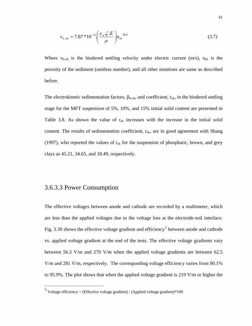
41
6.3911 ...
.10*87.7 ekw
ekh nE
v
= −
− µζε
(3.7)
Where vh-ek is the hindered settling velocity under electric current (m/s), nek is the
porosity of the sediment (unitless number), and all other notations are same as described
before.
The electrokinetic sedimentation factors, βh-ek, and coefficient, rek, in the hindered settling
stage for the MFT suspension of 5%, 10%, and 15% initial solid content are presented in
Table 3.8. As shown the value of rek increases with the increase in the initial solid
content. The results of sedimentation coefficient, rek, are in good agreement with Shang
(1997), who reported the values of rek for the suspension of phosphatic, brown, and grey
clays as 45.21, 34.65, and 18.49, respectively.
3.6.3.3 Power Consumption
The effective voltages between anode and cathode are recorded by a multimeter, which
are less than the applied voltages due to the voltage loss at the electrode-soil interface.
Fig. 3.30 shows the effective voltage gradient and efficiency5 between anode and cathode
vs. applied voltage gradient at the end of the tests. The effective voltage gradients vary
between 56.3 V/m and 270 V/m when the applied voltage gradients are between 62.5
V/m and 281 V/m, respectively. The corresponding voltage efficiency varies from 90.1%
to 95.9%. The plot shows that when the applied voltage gradient is 219 V/m or higher the
5 Voltage efficiency = (Effective voltage gradient) / (Applied voltage gradient)*100
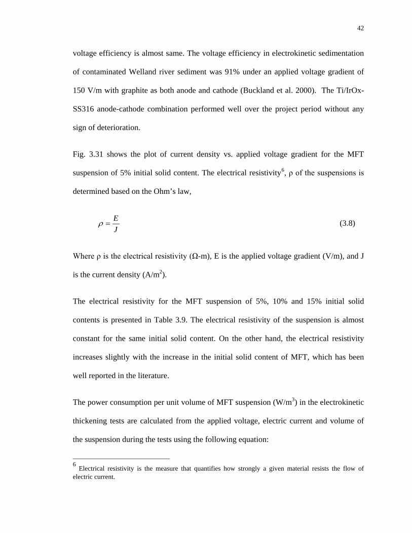
42
voltage efficiency is almost same. The voltage efficiency in electrokinetic sedimentation
of contaminated Welland river sediment was 91% under an applied voltage gradient of
150 V/m with graphite as both anode and cathode (Buckland et al. 2000). The Ti/IrOx-
SS316 anode-cathode combination performed well over the project period without any
sign of deterioration.
Fig. 3.31 shows the plot of current density vs. applied voltage gradient for the MFT
suspension of 5% initial solid content. The electrical resistivity6, ρ of the suspensions is
determined based on the Ohm’s law,
JE
=ρ (3.8)
Where ρ is the electrical resistivity (Ω-m), E is the applied voltage gradient (V/m), and J
is the current density (A/m2).
The electrical resistivity for the MFT suspension of 5%, 10% and 15% initial solid
contents is presented in Table 3.9. The electrical resistivity of the suspension is almost
constant for the same initial solid content. On the other hand, the electrical resistivity
increases slightly with the increase in the initial solid content of MFT, which has been
well reported in the literature.
The power consumption per unit volume of MFT suspension (W/m3) in the electrokinetic
thickening tests are calculated from the applied voltage, electric current and volume of
the suspension during the tests using the following equation:
6 Electrical resistivity is the measure that quantifies how strongly a given material resists the flow of electric current.
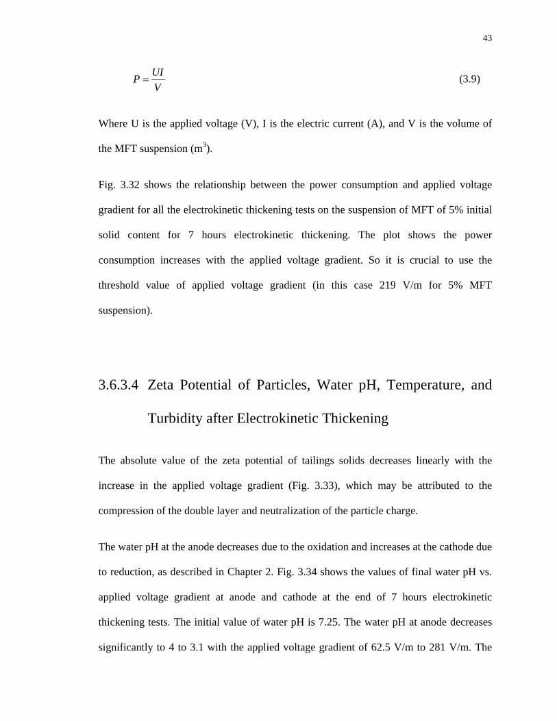
43
VUIP = (3.9)
Where U is the applied voltage (V), I is the electric current (A), and V is the volume of
the MFT suspension (m3).
Fig. 3.32 shows the relationship between the power consumption and applied voltage
gradient for all the electrokinetic thickening tests on the suspension of MFT of 5% initial
solid content for 7 hours electrokinetic thickening. The plot shows the power
consumption increases with the applied voltage gradient. So it is crucial to use the
threshold value of applied voltage gradient (in this case 219 V/m for 5% MFT
suspension).
3.6.3.4 Zeta Potential of Particles, Water pH, Temperature, and
Turbidity after Electrokinetic Thickening
The absolute value of the zeta potential of tailings solids decreases linearly with the
increase in the applied voltage gradient (Fig. 3.33), which may be attributed to the
compression of the double layer and neutralization of the particle charge.
The water pH at the anode decreases due to the oxidation and increases at the cathode due
to reduction, as described in Chapter 2. Fig. 3.34 shows the values of final water pH vs.
applied voltage gradient at anode and cathode at the end of 7 hours electrokinetic
thickening tests. The initial value of water pH is 7.25. The water pH at anode decreases
significantly to 4 to 3.1 with the applied voltage gradient of 62.5 V/m to 281 V/m. The
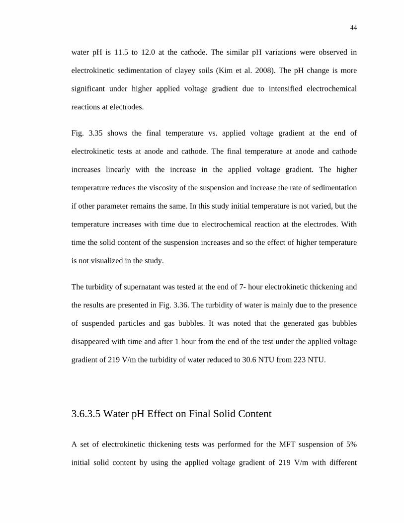
44
water pH is 11.5 to 12.0 at the cathode. The similar pH variations were observed in
electrokinetic sedimentation of clayey soils (Kim et al. 2008). The pH change is more
significant under higher applied voltage gradient due to intensified electrochemical
reactions at electrodes.
Fig. 3.35 shows the final temperature vs. applied voltage gradient at the end of
electrokinetic tests at anode and cathode. The final temperature at anode and cathode
increases linearly with the increase in the applied voltage gradient. The higher
temperature reduces the viscosity of the suspension and increase the rate of sedimentation
if other parameter remains the same. In this study initial temperature is not varied, but the
temperature increases with time due to electrochemical reaction at the electrodes. With
time the solid content of the suspension increases and so the effect of higher temperature
is not visualized in the study.
The turbidity of supernatant was tested at the end of 7- hour electrokinetic thickening and
the results are presented in Fig. 3.36. The turbidity of water is mainly due to the presence
of suspended particles and gas bubbles. It was noted that the generated gas bubbles
disappeared with time and after 1 hour from the end of the test under the applied voltage
gradient of 219 V/m the turbidity of water reduced to 30.6 NTU from 223 NTU.
3.6.3.5 Water pH Effect on Final Solid Content
A set of electrokinetic thickening tests was performed for the MFT suspension of 5%
initial solid content by using the applied voltage gradient of 219 V/m with different
45
suspension pH. The pH of the suspensions was adjusted by titration using 0.1MHCl and
0.1MNaOH. Fig. 3.37 shows the plot of height of mudline and final solid content vs.
suspension pH at the end of 7 hours testing under an applied voltage gradient of 219 V/m.
At the end of the tests, the final solid content at pH 7.25 (MFT suspension pH without
adjustment) was 18.75% while at pH 5 and 10.5 the solid content reached 16.79% and
19.2%, respectively. The effect of thickening is the best at higher suspensions pH, which
is attributed to the higher values of zeta potential.
It is observed that thickening of the MFT suspension lasted up to 4 hours from the start
and the final solid content reached 6.48% under 350 mg/l ferric chloride as the coagulant.
On the other hand, thickening by electrokinetics continued up to around 7 hours, and the
final solid content was 18.75% under the applied voltage gradient of 219 V/m. In
conclusion the electrokinetic thickening is 3 times more effective than coagulation in
terms of the final solid content of MFT.
3.7 Summary
In this chapter the mature fine oil sands tailings (MFT) is characterized for the physical,
chemical and geological properties, followed by description of detailed testing
procedures, as well as results and discussions of jar tests and cylinder coagulation tests.
The key investigation in this chapter is the electrokinetic thickening of MFT suspension.
The results of coagulation and electrokinetic thickening tests are presented, analyzed and
compared. The main findings are as follows:
46
a) The mature fine oil sands tailings contain 82.5% silt and 17.5% clay-sized solids
and have a natural water content of 158%. The plasticity index of MFT was 18.4%, and
hence it is categorized as elastic silt. The major minerals in the mature fine oil sands
tailings are found to be quartz, illite, and kaolinite. The pore water pH and electrical
conductivity (EC) are found as 8.19 and 3.51 mS/cm, respectively.
b) In the series of jar experiments, ferric chloride at 350 mg/l generated the best
coagulation effect in terms of the final position of mudline and final solid content among
different coagulants studied.
c) Ferric chloride produced the best settling effect in the MFT suspensions at 350
mg/l concentration, and the final solid content was 6.48% for the MFT suspension of 5%
initial solid content after 4 hours in cylinder coagulation tests.
d) In electrokinetic thickening test, the final solid content reached 18.75% from 5%
initial solid content of the MFT suspension under the applied voltage gradient of 219 V/m
after 7 hours. The increase in the applied voltage gradient increased the final solid
content, and free settling velocity, and reduced the duration of free settling.
e) The equations of sedimentation velocity in the free settling and hindered settling
stages are validated using the experimental data.
f) The voltage efficiency ranges from 90.1% to 95.9% under the applied voltage
gradient of 62.5 V/m to 281 V/m, respectively, for the MFT suspension of 5% initial
solid content. The power consumption in the electrokinetic tests varies from 0.271
KW/m3 to 6.15 KW/m3. The electrical resistivity of the suspension is almost constant for
the same initial solid content and increases slightly with the increase in the initial solid
content of the suspension.
47
g) The final turbidity (without pH adjustment) of the supernatant is 14.4 NTU and
30.6 NTU under coagulation and electrokinetics, respectively and the corresponding zeta
potential of particles is -22.6 mV and -14.7 mV.
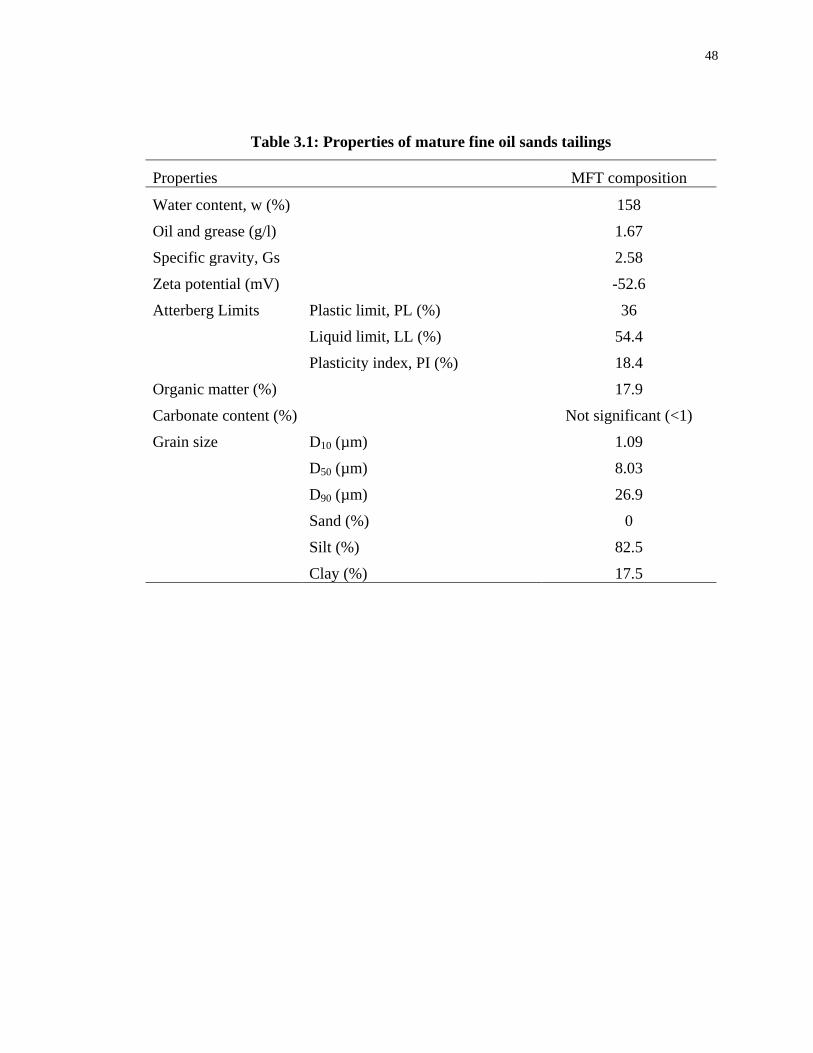
48
Table 3.1: Properties of mature fine oil sands tailings
Properties MFT composition
Water content, w (%) 158
Oil and grease (g/l) 1.67
Specific gravity, Gs 2.58
Zeta potential (mV) -52.6
Atterberg Limits Plastic limit, PL (%) 36
Liquid limit, LL (%) 54.4
Plasticity index, PI (%) 18.4
Organic matter (%) 17.9
Carbonate content (%) Not significant (<1)
Grain size D10 (µm) 1.09
D50 (µm) 8.03
D90 (µm) 26.9
Sand (%) 0
Silt (%) 82.5
Clay (%) 17.5

49
Table 3.2: Chemical analysis of pore water of mature fine oil sands tailings
Cations Concentrations (mg/l)
Na 600
Mg 9.03
K 19.7
Ca 9.74
Al 0.04
V 0.01
Fe 0.02
Ni 0.01
Cu 0.13
Zn 0.01
Rb 0.08
Sr 0.35
Ba 0.1
Pb 0.01
Anions Concentrations (mg/l)
Cl– 279
SO42– 29.1
NO3– 2.6
OH– 0.026
Water pH 8.19
EC of MFT (mS/cm) 3.51
EC of MFT suspension (µS/cm):
5% initial solid content
10% initial solid content
15% initial solid content
511
751
997

50
Table 3.3: Conditions of jar experiments
Conditions
No. of beakers 6
Size of beakers 500 ml
9 cm height
Beaker making material Borosilicate glass
No. of mixing blades 6
Revolution of mixing blades 100 rpm (rapid mixing)
20 rpm (slow mixing)
Mixing periods 2 min (rapid mixing)
20 min (slow mixing)
Settlement period 60 min
Variables in tests Initial solid content
Coagulants
Coagulant dosage
pH
Initial solid content 5%, 10%, 15%
Types of coagulants Alum (Al2(SO4)3.18H2O)
Aluminum chloride (AlCl3)
Ferric chloride (FeCl3)
Method of coagulants mixing By syringe
Coagulant dosage in the suspension Varies between 0 and 700 mg/l
Recorded room temperature during tests 20 to 22 °C
Observation tools Height of mudline from the bottom of the beaker
Final solid content

51
Table 3.4: Conditions of coagulation tests at cylinder
Conditions
No. of cylinders 7
Size of cylinders 1 L
35 cm height
Cylinder making material Borosilicate glass
Thickening period 4 hr
Initial solid content 5%
Type of coagulant Ferric chloride (FeCl3)
Method of coagulants mixing By syringe
Coagulant dosage in the suspension 0, 100 mg/l, 200 mg/l, 300 mg/l, 350 mg/l, 400 mg/l, and 450 mg/l
Recorded room temperature during tests 20 to 22 °C
Observation tools Height of mudline from the bottom of the beaker
Turbidity of clear water at the top
Final solid content of the sediment at the bottom
Zeta potential (with varying pH only)
Electric conductivity (with varying pH only)

52
Table 3.5: Conditions of electrokinetic thickening tests
Conditions
Size of electrokinetic thickening column 1 L
16.8 cm height
8.9 cm inside diameter
Column making materials Plexiglass
Type of electrodes Anode (titanium coated with iridium oxide)
Cathode (stainless steel mesh)
0.063 ̋ in thickness and 30% in open area (both electrode)
Vertical distance between electrodes 16 cm
Power supply DC power supply (Hewlett Packard 6545-J05)
Variables in tests Initial solid content
Applied voltage
Initial solid content 5%, 10%, 15%
Applied voltage 0, 10 V, 20 V, 30 V, 35 V, 40 V, 45 V
Thickening period 7 hr
Recorded room temperature during tests 16.5 to 18 °C
Observation tools Height of mudline from the bottom of the beaker
Turbidity of supernatant at the top
Final solid content of the sediment at the bottom
Electric current
Change of pH at anode and cathode
Change of temperature at anode and cathode
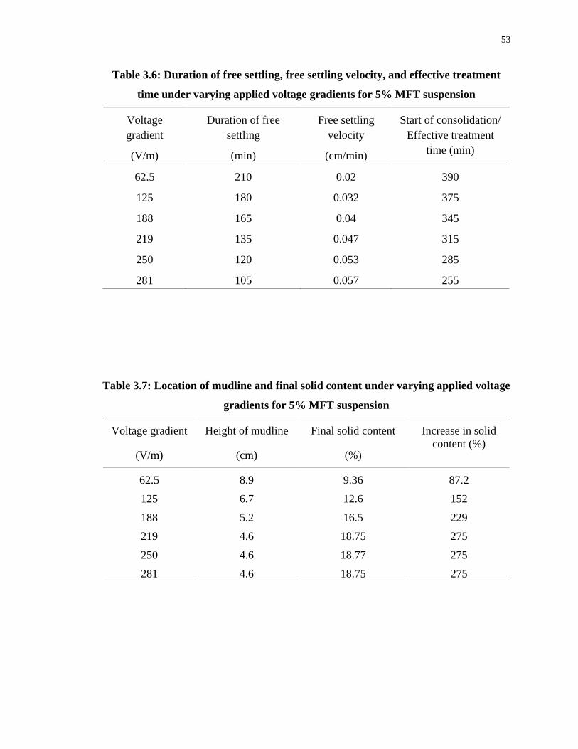
53
Table 3.6: Duration of free settling, free settling velocity, and effective treatment
time under varying applied voltage gradients for 5% MFT suspension
Voltage gradient
(V/m)
Duration of free settling
(min)
Free settling velocity
(cm/min)
Start of consolidation/ Effective treatment
time (min)
62.5 210 0.02 390
125 180 0.032 375
188 165 0.04 345
219 135 0.047 315
250 120 0.053 285
281 105 0.057 255
Table 3.7: Location of mudline and final solid content under varying applied voltage
gradients for 5% MFT suspension
Voltage gradient
(V/m)
Height of mudline
(cm)
Final solid content
(%)
Increase in solid content (%)
62.5 8.9 9.36 87.2
125 6.7 12.6 152
188 5.2 16.5 229
219 4.6 18.75 275
250 4.6 18.77 275
281 4.6 18.75 275
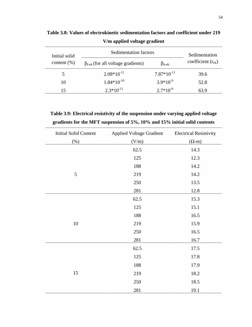
54
Table 3.8: Values of electrokinetic sedimentation factors and coefficient under 219
V/m applied voltage gradient
Initial solid content (%)
Sedimentation factors Sedimentation coefficient (rek) βf-ek (for all voltage gradients) βh-ek
5 2.08*10-11 7.87*10-11 39.6
10 1.84*10-10 3.9*10-9 52.8
15 2.3*10-11 2.7*10-9 63.9
Table 3.9: Electrical resistivity of the suspension under varying applied voltage
gradients for the MFT suspension of 5%, 10% and 15% initial solid contents
Initial Solid Content
(%)
Applied Voltage Gradient
(V/m)
Electrical Resistivity
(Ω-m)
5
62.5 14.3
125 12.3
188 14.2
219 14.2
250 13.5
281 12.8
10
62.5 15.3
125 15.1
188 16.5
219 15.9
250 16.5
281 16.7
15
62.5 17.5
125 17.8
188 17.9
219 18.2
250 18.5
281 19.1
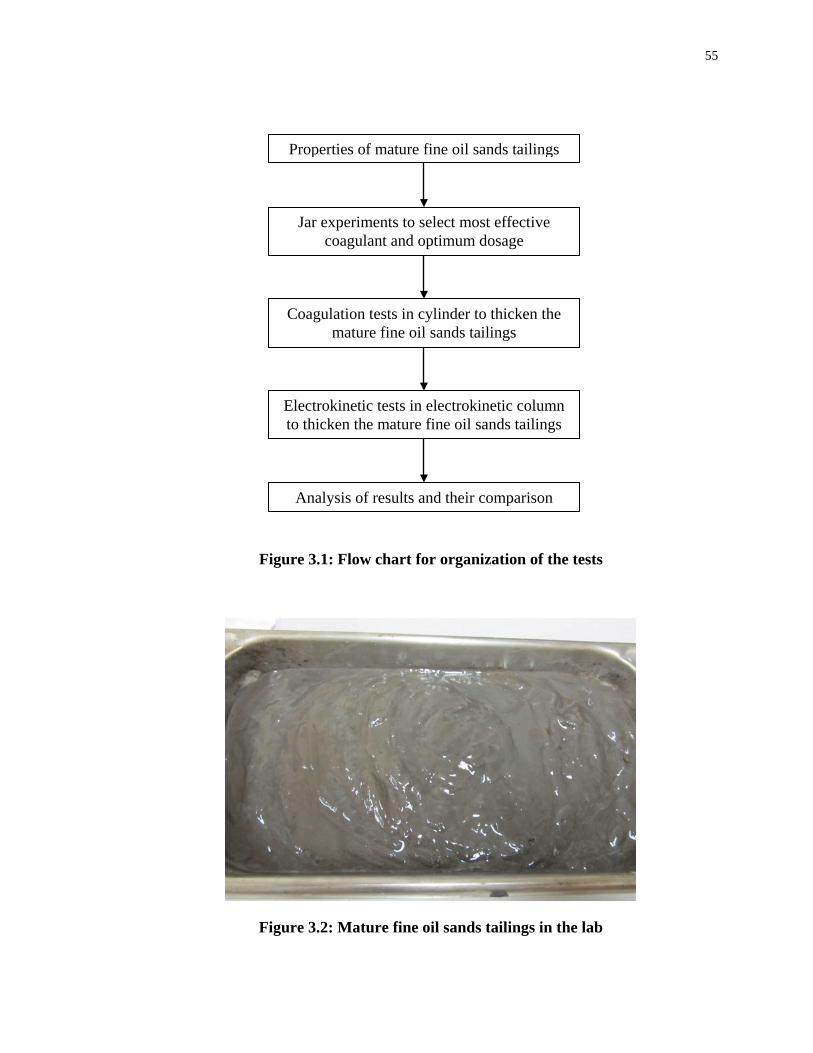
55
Figure 3.1: Flow chart for organization of the tests
Figure 3.2: Mature fine oil sands tailings in the lab
Properties of mature fine oil sands tailings
Jar experiments to select most effective coagulant and optimum dosage
Coagulation tests in cylinder to thicken the mature fine oil sands tailings
Electrokinetic tests in electrokinetic column to thicken the mature fine oil sands tailings
Analysis of results and their comparison
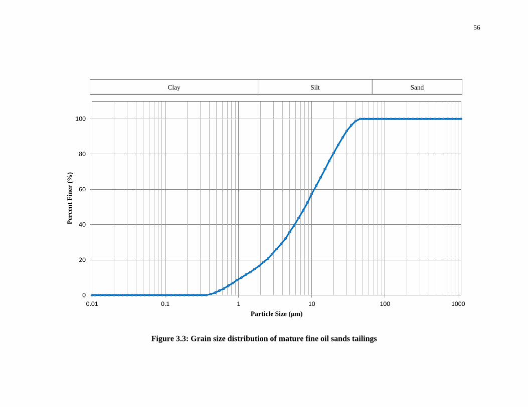
56
Clay Silt Sand
0
20
40
60
80
100
0.01 0.1 1 10 100 1000
Perc
ent F
iner
(%)
Particle Size (μm)
Figure 3.3: Grain size distribution of mature fine oil sands tailings

57
0
1000
2000
3000
4000
5000
6000
7000
0 10 20 30 40 50 60 70
Cou
nts
Degrees (2θ)
Illite K
aolin
ite
Qua
rtz
Qua
rtz
Qua
rtz/Il
lite
Kao
linite
Qur
atz
Figure 3.4: X-ray diffraction on pulverized mature fine oil sands tailings
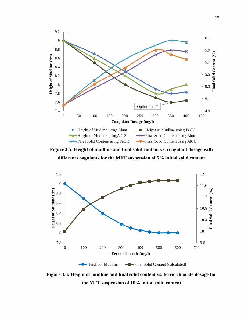
58
4.9
5.1
5.3
5.5
5.7
5.9
6.1
7.4
7.6
7.8
8
8.2
8.4
8.6
8.8
9
9.2
0 50 100 150 200 250 300 350 400 450
Fina
l Sol
id C
onte
nt (
%)
Hei
ght o
f Mud
line
(cm
)
Coagulant Dosage (mg/l)
Height of Mudline using Alum Height of Mudline using FeCl3Height of Mudline usingAlCl3 Final Solid Content using AlumFinal Solid Content using FeCl3 Final Solid Content using AlCl3
Optimum
Figure 3.5: Height of mudline and final solid content vs. coagulant dosage with
different coagulants for the MFT suspension of 5% initial solid content
9.6
10
10.4
10.8
11.2
11.6
12
7.8
8
8.2
8.4
8.6
8.8
9
9.2
0 100 200 300 400 500 600 700
Fina
l Sol
id C
onte
nt (%
)
Hei
ght o
f Mud
line
(cm
)
Ferric Chloride (mg/l)
Height of Mudline Final Solid Content (calculated)
Figure 3.6: Height of mudline and final solid content vs. ferric chloride dosage for
the MFT suspension of 10% initial solid content
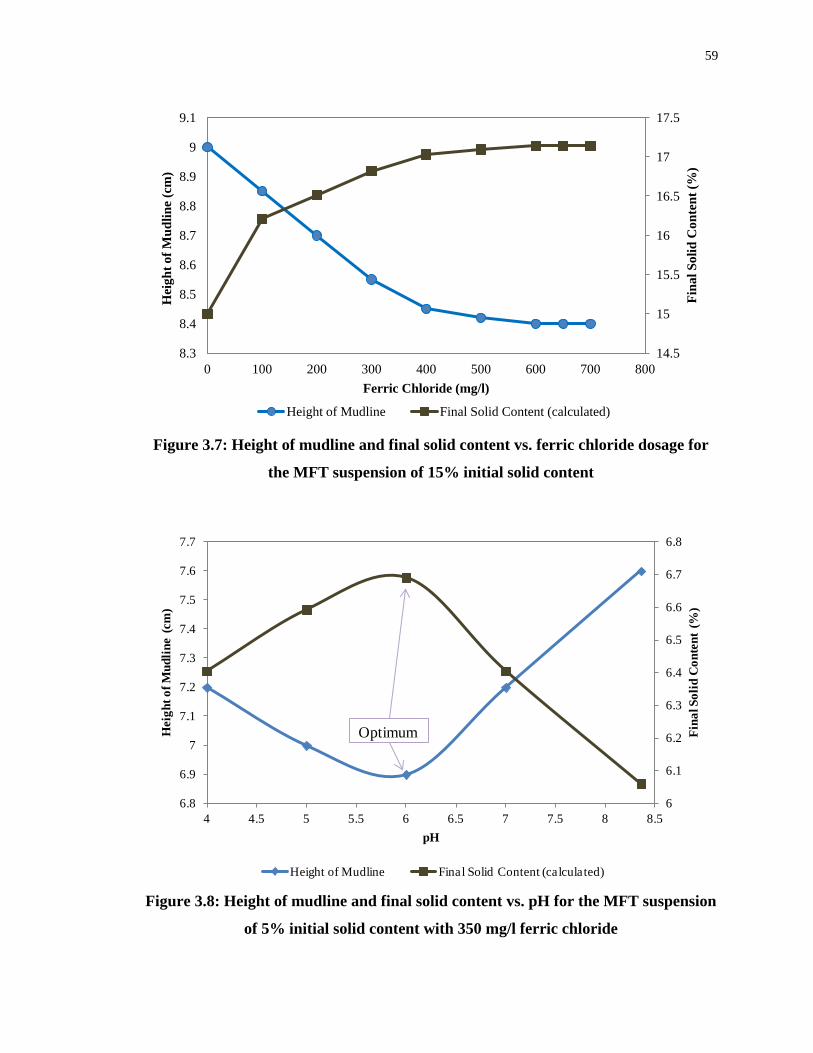
59
14.5
15
15.5
16
16.5
17
17.5
8.3
8.4
8.5
8.6
8.7
8.8
8.9
9
9.1
0 100 200 300 400 500 600 700 800
Fina
l Sol
id C
onte
nt (%
)
Hei
ght o
f Mud
line
(cm
)
Ferric Chloride (mg/l)
Height of Mudline Final Solid Content (calculated)
Figure 3.7: Height of mudline and final solid content vs. ferric chloride dosage for
the MFT suspension of 15% initial solid content
6
6.1
6.2
6.3
6.4
6.5
6.6
6.7
6.8
6.8
6.9
7
7.1
7.2
7.3
7.4
7.5
7.6
7.7
4 4.5 5 5.5 6 6.5 7 7.5 8 8.5
Fina
l Sol
id C
onte
nt (
%)
Hei
ght o
f Mud
line
(cm
)
pH
Height of Mudline Final Solid Content (calculated)
Optimum
Figure 3.8: Height of mudline and final solid content vs. pH for the MFT suspension
of 5% initial solid content with 350 mg/l ferric chloride

60
27
29
31
33
35
37
0 30 60 90 120 150 180 210 240
Hei
ght o
f Mud
line
(cm
)
Time (minute)
0 (Control)
100 mg/l
200 mg/l
300 mg/l
350 mg/l
400 mg/l
450 mg/l
Figure 3.9: Height of mudline vs. time under varying concentrations of ferric chloride

61
0
0.01
0.02
0.03
0.04
0.05
0.06
0.07
0.08
0 50 100 150 200 250
Settl
ing
Vel
ocity
(cm
/min
)
Time (min)
0 (Control)
100 mg/l FeCl3
200 mg/l FeCl3
300 mg/l FeCl3
350 mg/l FeCl3
400 mg/l FeCl3
450 mg/l FeCl3
Free Settling Hindered Settling Start of Consolidation
(For 350 mg/l FeCl3)
Figure 3.10: Settling velocity vs. time under varying concentrations of ferric chloride
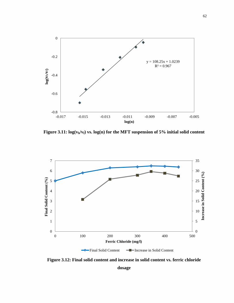
62
y = 108.25x + 1.0239R² = 0.967
-0.8
-0.6
-0.4
-0.2
0
-0.017 -0.015 -0.013 -0.011 -0.009 -0.007 -0.005
log(
vh/v
f)
log(n)
Figure 3.11: log(vh/vf) vs. log(n) for the MFT suspension of 5% initial solid content
0
5
10
15
20
25
30
35
0
1
2
3
4
5
6
7
0 100 200 300 400 500
Incr
ease
in S
olid
Con
tent
(%)
Fina
l Sol
id C
onte
nt (%
)
Ferric Chloride (mg/l)
Final Solid Content Increase in Solid Content
Figure 3.12: Final solid content and increase in solid content vs. ferric chloride
dosage

63
0
5
10
15
20
25
30
35
100 200 300 350 400 450
Tur
bidi
ty (N
TU
)
Ferric Chloride (mg/l)
Figure 3.13: Turbidity of supernatant at the top of cylinder for different ferric
chloride dosage
0
200
400
600
800
1000
100 200 300 350 400 450
Tot
al S
olid
s (m
g/l)
Ferric Chloride (mg/l)
Figure 3.14: Total solids of supernatant at the top of cylinder for different ferric
chloride dosage
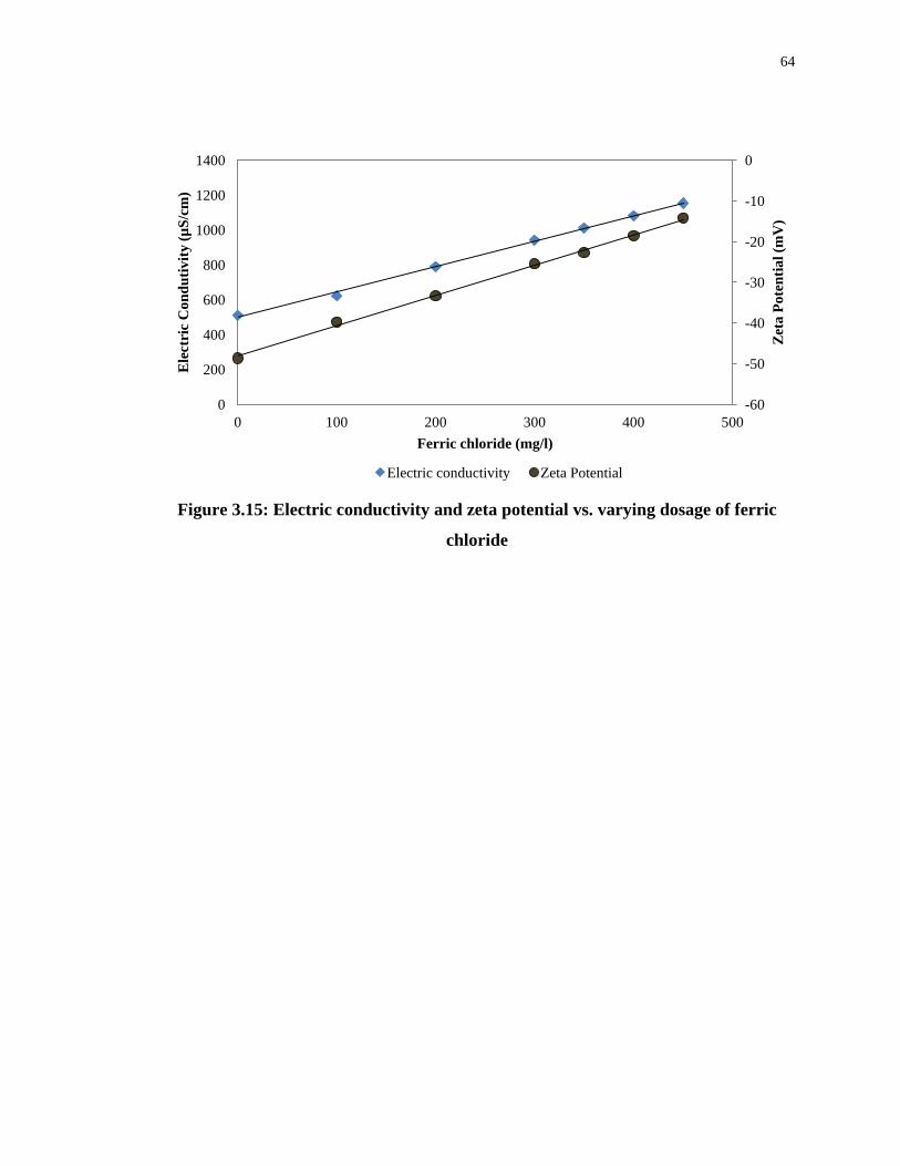
64
-60
-50
-40
-30
-20
-10
0
0
200
400
600
800
1000
1200
1400
0 100 200 300 400 500
Zeta
Pot
entia
l (m
V)
Ele
ctri
c C
ondu
tivity
(µS/
cm)
Ferric chloride (mg/l)
Electric conductivity Zeta Potential
Figure 3.15: Electric conductivity and zeta potential vs. varying dosage of ferric
chloride

65
25
27
29
31
33
35
37
0 50 100 150 200 250
Hei
ght o
f Mud
line
(cm
)
Time (min)
pH 4
pH 5
pH 6
pH 7.25
pH 8.36
Figure 3.16: Height of mudline vs. time under varying pH of MFT suspension of 5% initial solid content
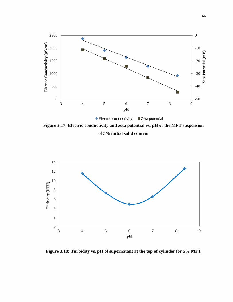
66
-50
-40
-30
-20
-10
0
0
500
1000
1500
2000
2500
3 4 5 6 7 8 9
Zeta
Pot
entia
l (m
V)
Elec
tric
Con
cuct
ivity
(µS/
cm)
pH
Electric conductivity Zeta potential
Figure 3.17: Electric conductivity and zeta potential vs. pH of the MFT suspension
of 5% initial solid content
0
2
4
6
8
10
12
14
3 4 5 6 7 8 9
Tur
bidi
ty (N
TU
)
pH
Figure 3.18: Turbidity vs. pH of supernatant at the top of cylinder for 5% MFT
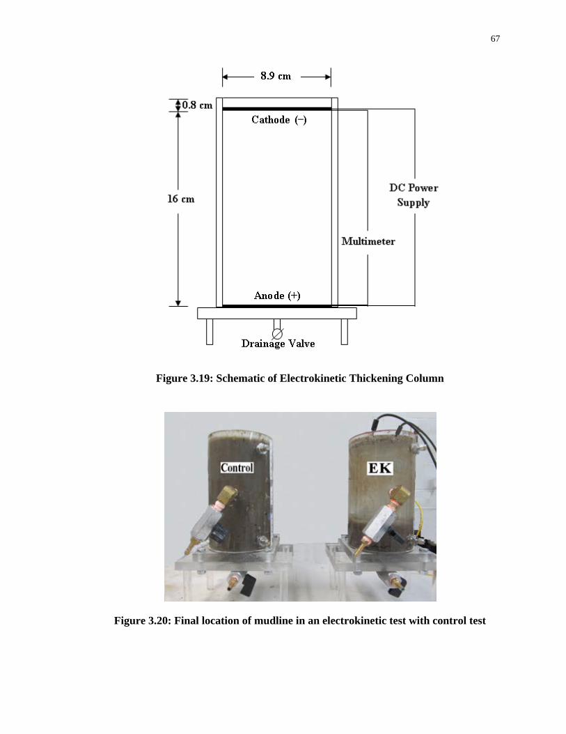
67
Figure 3.19: Schematic of Electrokinetic Thickening Column
Figure 3.20: Final location of mudline in an electrokinetic test with control test

68
2
4
6
8
10
12
14
16
18
0 50 100 150 200 250 300 350 400 450
Hei
ght o
f mud
line
(cm
)
Time (min)
0 V/m (Control)
62.5 V/m
125 V/m
188 V/m
219 V/m
250 V/m
281 V/m
Figure 3.21: Height of mudline vs. time for the MFT suspension of 5% initial solid content under varying applied voltage
gradients

69
6
8
10
12
14
16
18
0 50 100 150 200 250 300 350 400 450
Hei
ght o
f mud
line
(cm
)
Time (min)
0 V/m (Control)
62.5 V/m
125 V/m
188 V/m
219 V/m
250 V/m
281 V/m
Figure 3.22: Height of mudline vs. time for the MFT suspension of 10% initial solid content under varying applied voltage
gradients
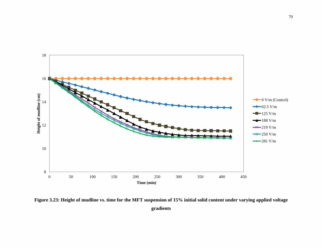
70
8
10
12
14
16
18
0 50 100 150 200 250 300 350 400 450
Hei
ght o
f mud
line
(cm
)
Time (min)
0 V/m (Control)
62.5 V/m
125 V/m
188 V/m
219 V/m
250 V/m
281 V/m
Figure 3.23: Height of mudline vs. time for the MFT suspension of 15% initial solid content under varying applied voltage
gradients
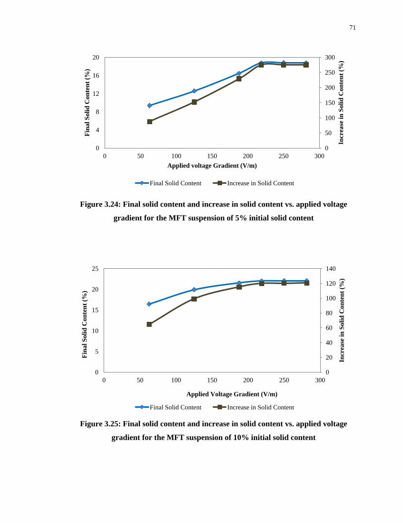
71
0
50
100
150
200
250
300
0
4
8
12
16
20
0 50 100 150 200 250 300
Incr
ease
in S
olid
Con
tent
(%)
Fina
l Sol
id C
onte
nt (%
)
Applied voltage Gradient (V/m)
Final Solid Content Increase in Solid Content
Figure 3.24: Final solid content and increase in solid content vs. applied voltage
gradient for the MFT suspension of 5% initial solid content
0
20
40
60
80
100
120
140
0
5
10
15
20
25
0 50 100 150 200 250 300
Incr
ease
in S
olid
Con
tent
(%)
Fina
l Sol
id C
onte
nt (%
)
Applied Voltage Gradient (V/m)
Final Solid Content Increase in Solid Content
Figure 3.25: Final solid content and increase in solid content vs. applied voltage
gradient for the MFT suspension of 10% initial solid content

72
10
20
30
40
50
60
70
80
0
5
10
15
20
25
30
0 50 100 150 200 250 300
Incr
ease
in S
olid
Con
tent
(%)
Fina
l Sol
id C
onte
nt (%
)
Applied Voltage Gradient (V/m)
Final Solid Content Increase in Solid Content
Figure 3.26: Final solid content and increase in solid content vs. applied voltage
gradient for the MFT suspension of 15% initial solid content

73
0
0.01
0.02
0.03
0.04
0.05
0.06
0 50 100 150 200 250 300 350 400 450
Settl
ing
Vel
ocity
(cm
/min
)
Time (min)
188 V/m
219 V/m
250 V/m
281 V/m
Free Settling
Hindered Settling Start of Consolidation(For 219 V/m)
Figure 3.27: Settling velocity vs. time for the MFT suspension of 5% initial solid content under varying applied voltage
gradients

74
vf-ek = 0.0002E + 0.0097R² = 0.995
0
0.01
0.02
0.03
0.04
0.05
0.06
0.07
0 50 100 150 200 250 300
Free
Set
tling
Vel
ocity
(cm
/min
)
Applied Voltage Gradient (V/m)
Figure 3.28: Relationship between free settling velocity and applied voltage gradient
for 5% MFT
y = 39.601x + 0.578R² = 0.9899
-0.4
-0.35
-0.3
-0.25
-0.2
-0.15
-0.1
-0.05
0
-0.026 -0.024 -0.022 -0.02 -0.018 -0.016 -0.014 -0.012 -0.01
log
(vh-
ek/v
f-ek
)
log (nek)
Figure 3.29: log (vh-ek/vf-ek) vs. log (nek) for 5% MFT under 219 V/m applied voltage
gradient
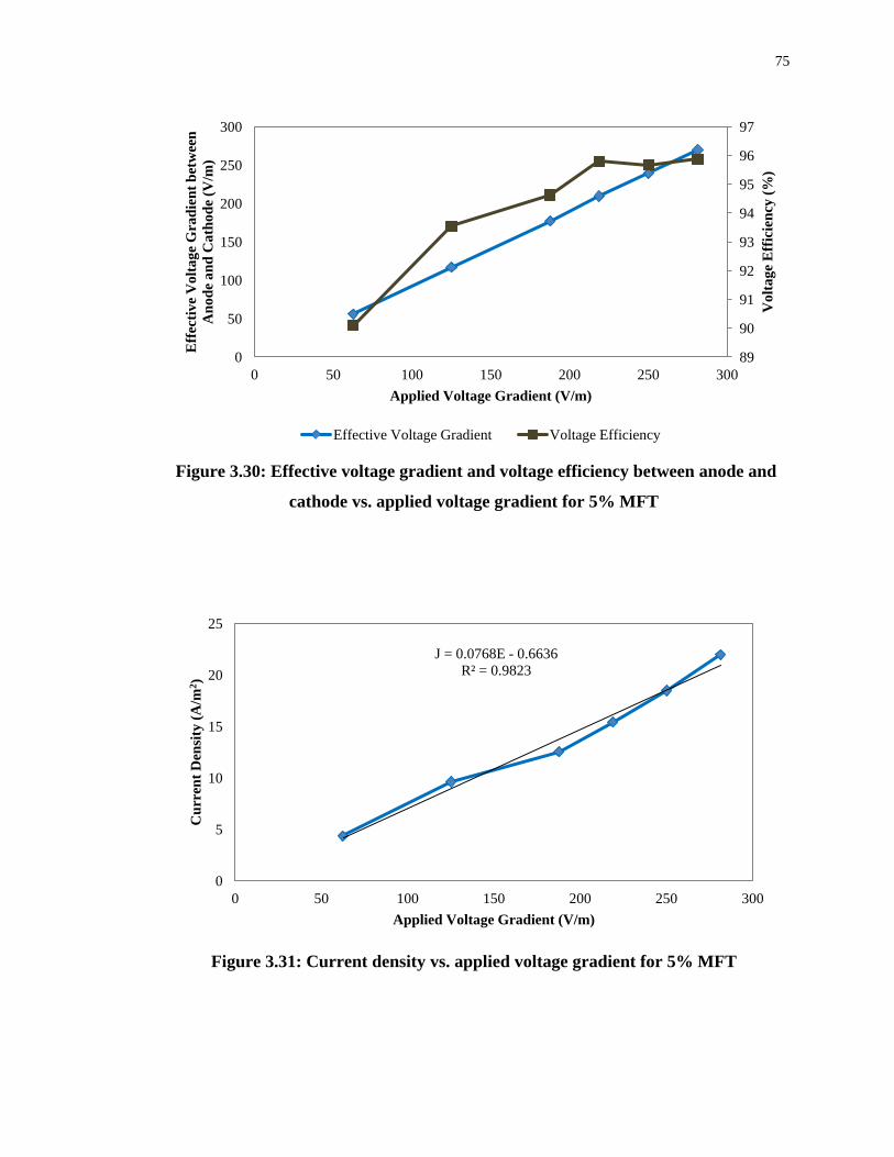
75
89
90
91
92
93
94
95
96
97
0
50
100
150
200
250
300
0 50 100 150 200 250 300
Vol
tage
Eff
icie
ncy
(%)
Eff
ectiv
e V
olta
ge G
radi
ent b
etw
een
Ano
de a
nd C
atho
de (V
/m)
Applied Voltage Gradient (V/m)
Effective Voltage Gradient Voltage Efficiency
Figure 3.30: Effective voltage gradient and voltage efficiency between anode and
cathode vs. applied voltage gradient for 5% MFT
J = 0.0768E - 0.6636R² = 0.9823
0
5
10
15
20
25
0 50 100 150 200 250 300
Cur
rent
Den
sity
(A/m
2 )
Applied Voltage Gradient (V/m)
Figure 3.31: Current density vs. applied voltage gradient for 5% MFT

76
0
1
2
3
4
5
6
7
0 50 100 150 200 250 300
Pow
er C
onsu
mpt
ion
(KW
/m3 )
Applied Voltage Gradient (V/m)
Figure 3.32: Power consumption vs. applied voltage gradient for 5% MFT
-35
-30
-25
-20
-15
-10
-50 50 100 150 200 250 300
Zeta
Pot
entia
l (m
V)
Applied Voltage Gradient (V/m)
Figure 3.33: Final zeta potential of particles vs. applied voltage gradient for 5%
MFT
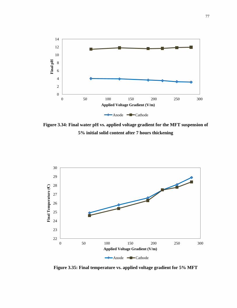
77
0
2
4
6
8
10
12
14
0 50 100 150 200 250 300
Fina
l pH
Applied Voltage Gradient (V/m)
Anode Cathode
Figure 3.34: Final water pH vs. applied voltage gradient for the MFT suspension of
5% initial solid content after 7 hours thickening
22
23
24
25
26
27
28
29
30
0 50 100 150 200 250 300
Fina
l Tem
pera
ture
(ͦͦC)
Applied Voltage Gradient (V/m)
Anode Cathode
Figure 3.35: Final temperature vs. applied voltage gradient for 5% MFT
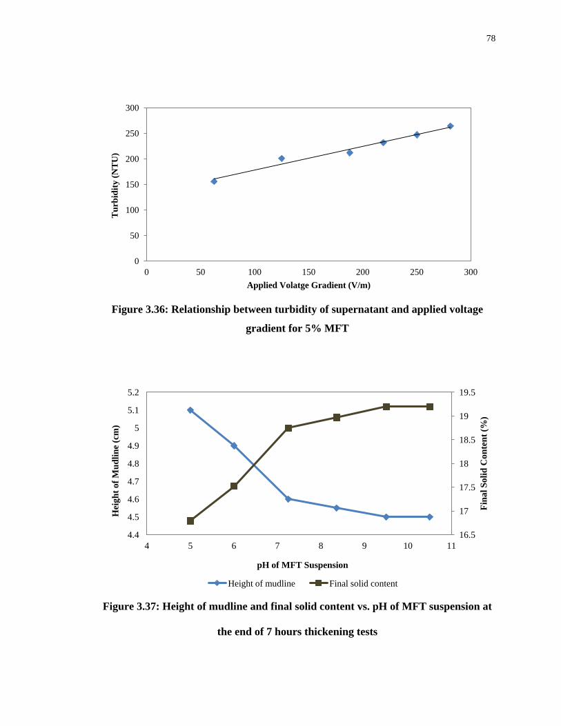
78
0
50
100
150
200
250
300
0 50 100 150 200 250 300
Tur
bidi
ty (N
TU
)
Applied Volatge Gradient (V/m)
Figure 3.36: Relationship between turbidity of supernatant and applied voltage
gradient for 5% MFT
16.5
17
17.5
18
18.5
19
19.5
4.4
4.5
4.6
4.7
4.8
4.9
5
5.1
5.2
4 5 6 7 8 9 10 11
Fina
l Sol
id C
onte
nt (%
)
Hei
ght o
f Mud
line
(cm
)
pH of MFT Suspension
Height of mudline Final solid content
Figure 3.37: Height of mudline and final solid content vs. pH of MFT suspension at
the end of 7 hours thickening tests

79
CHAPTER 4 COMBINED APPLICATION OF COAGULATION
AND ELECTROKINETIC THICKENING AND
OPTIMIZATION OF RESULTS BY ANOVA
4.1 Introduction
The study on the combined effects of coagulation and electrokinetic thickening is
presented in this chapter. It is found in chapter 3 that the thickening with both coagulation
and electrokinetics are the most effective on the suspension of low initial solid content
(5%). This combined study consists of two phases: (a) study the combined effect of a
continuous electric voltage gradient and coagulant (350 mg/l ferric chloride), and (b)
study the effect of an intermittent voltage in combination with ferric chloride. Finally
regression models are developed to relate applied voltage gradient and final solid content
for electrokinetic thickening and combined study.
The purpose of this study is to observe the effect of these parameters on increasing the
final solid content of MFT. The mudline position, effective voltage gradient and voltage
efficiency, power consumption, effective treatment time, the zeta potential of particles,
and turbidity of supernatant are examined. The results of the combined tests are
compared with that of the electrokinetic thickening. The study of the intermittent applied
voltage gradient with ferric chloride focuses on the settling velocity and final solid
content.

80
The regression models using response surface method are developed for electrokinetic
thickening and combined application of coagulation and electrokinetic thickening, and
their significance are examined by F-test. Moreover, the significance of independent
process variables on the models is also judged using t-test values. The outcomes of the
models are presented in contour plots showing the influences of independent variables on
the optimization of response variables.
4.2 Combined Application of Coagulation and Electrokinetic
Thickening
4.2.1 Testing Procedure
The same columns for electrokinetic thickening described in Chapter 3 are used for
combined coagulation and electrokinetic tests. The coagulation and electrophoresis are
applied simultaneously to counteract the reduction of zeta potential as possible by
coagulant. The conditions of combined tests are summarized in Table 4.1. The prepared
MFT suspension of 5% initial solid content is used for the combined tests. Ferric chloride
at 350 mg/l is found as the optimal coagulant in jar and cylinder coagulation tests
(Chapter 3). Hence, the combined coagulation and electrokinetic tests are carried out
using 350 mg/l ferric chloride and application of an applied voltage gradient for 7 hours.
The MFT suspension is poured into the testing column. The applied voltages gradients
vary between 0 and 281 V/m, as presented in Table 4.1. In all tests the location of
mudline, effective voltage gradient between the anode and cathode, and electric current
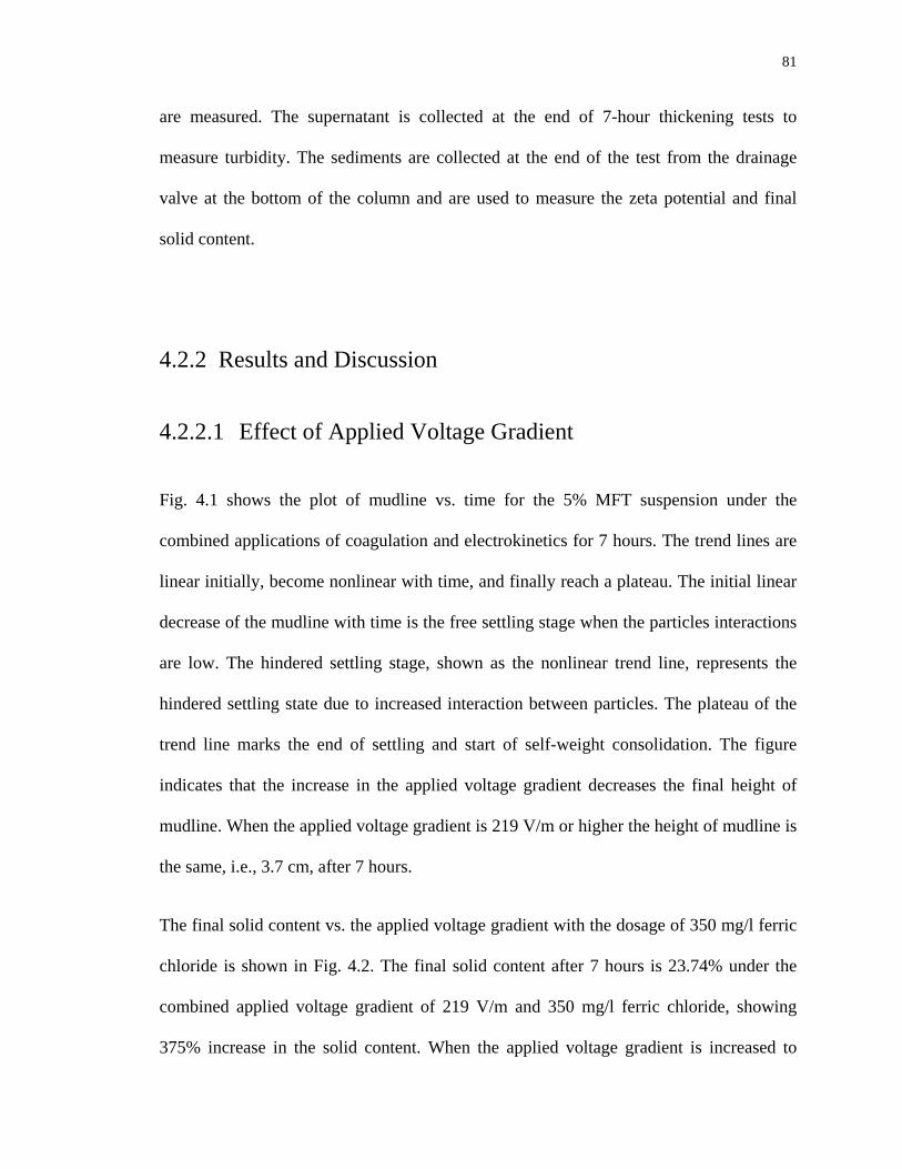
81
are measured. The supernatant is collected at the end of 7-hour thickening tests to
measure turbidity. The sediments are collected at the end of the test from the drainage
valve at the bottom of the column and are used to measure the zeta potential and final
solid content.
4.2.2 Results and Discussion
4.2.2.1 Effect of Applied Voltage Gradient
Fig. 4.1 shows the plot of mudline vs. time for the 5% MFT suspension under the
combined applications of coagulation and electrokinetics for 7 hours. The trend lines are
linear initially, become nonlinear with time, and finally reach a plateau. The initial linear
decrease of the mudline with time is the free settling stage when the particles interactions
are low. The hindered settling stage, shown as the nonlinear trend line, represents the
hindered settling state due to increased interaction between particles. The plateau of the
trend line marks the end of settling and start of self-weight consolidation. The figure
indicates that the increase in the applied voltage gradient decreases the final height of
mudline. When the applied voltage gradient is 219 V/m or higher the height of mudline is
the same, i.e., 3.7 cm, after 7 hours.
The final solid content vs. the applied voltage gradient with the dosage of 350 mg/l ferric
chloride is shown in Fig. 4.2. The final solid content after 7 hours is 23.74% under the
combined applied voltage gradient of 219 V/m and 350 mg/l ferric chloride, showing
375% increase in the solid content. When the applied voltage gradient is increased to

82
higher than 219 V/m, the final solid contents do not further increase. The individual
application of coagulation and electrokinetics reaches the final solid content of MFT
suspension to 6.48% and 18.75%, respectively, from an initial of 5% (discussed in
Chapter 3). The combined application of electrokinetics and coagulation produces 1.3
times and 3.7 times more concentrated sediments than that of the individual application
of electrokinetics and coagulation, respectively. The results are consistent with the results
of Buckland et al. (2000) who reported the combined application of 150 V/m applied
voltage gradient and 40 mg/l ferric chloride yielded 1.2 times and 1.3 times more
concentrated sediment than those of their individual effect.
The average settling velocity is calculated using Equation 3.1 in Fig. 4.1. Fig. 4.3 shows
the settling velocity vs. time under the combined coagulation and electrokinetic
thickening. The settling velocity is constant in the free settling stage, and the zero settling
velocity at the end indicates the start of self weight consolidation. The details of free
settling velocity are summarized in Table 4.2. The free settling velocity increases with
the increase in the applied voltage gradient. On the other hand, an increase in the applied
voltage gradient reduces the time of free settling, leading to the earlier start of the self-
weight consolidation. The average free settling velocity of the suspension under the ferric
chloride only (control test) is 0.02 cm/min, while with the applied voltage gradient of 219
V/m, the free settling velocity is 0.06 cm/min. The increase in free settling velocity is
attributed to the applied voltage gradient. The similar result of electrokinetic thickening
velocity (0.047 cm/min) was found in Chapter 3 under the electric current only. The
effective treatment time for different applied voltage gradients combined with 350 mg/l
of ferric chloride is presented in Table 4.2, and the effective thickening time decreases

83
with the increase in the applied voltage gradient. The settling under combined
application is more rapid comparing to that of the lone effect of electrophoresis. In
conclusion, electrokinetic thickening combined with coagulation can reduce the treatment
time, which saves energy.
4.2.2.2 Power Consumption
The effective voltage gradients between the anode and cathode are recorded from the
multimeter. The plot of the effective voltage gradient and voltage efficiency vs. the
applied voltage gradient is shown in Fig. 4.4. The effective voltage gradient increases
linearly with the rise in applied voltage gradient. The voltage efficiency increases with
increasing the applied voltage gradients (up to 219 V/m) combined with 350 mg/l ferric
chloride, ranging from 92.4% to 97%. The voltage efficiency varied between 90.1% and
95.9% under the application of applied voltage gradient only, discussed in Chapter 3,
which demonstrates that the Ti/IrOx-SS316 anode-cathode combination performs well in
the presence of ferric chloride. It is also noticed from the plot that the voltage efficiency
is almost constant when the applied voltage gradient is 219 V/m or higher.
The electric current through the MFT suspension is recorded. The current density varies
linearly with the change in applied voltage gradient and the results are plotted in Fig. 4.5.
The electrical resistivity, ρ of the suspensions containing 5% initial solid content under
different applied voltage gradients combined with ferric chloride is determined from
applied voltage gradient, E and current density, J using Equation 3.2 and the results are
84
summarized in Table 4.3. It shows the suspensions electrical resistivity is almost constant
with varying applied voltage gradient. The electrical resistivity of the suspension is 13.6
Ω-m, which is marginally lower than that suspension without coagulant (14.16 Ω-m).
The power consumption (W/m3) of the combined coagulation and electrokinetic
thickening tests are calculated from the volume of MFT suspension (m3), applied voltage
(V) and electric current (A) during the tests using Equation 3.9. The plot of power
consumption vs. applied voltage gradient combined with 350 mg/l ferric chloride for 7
hours electrokinetic thickening is shown in Fig. 4.6. The power consumption increases
with the increase in applied voltage gradient. The power consumption in the combined
coagulation electrokinetic thickening is higher than that of electrokinetics only. The
increased electrical conductivity due to the addition of ferric chloride increases the flow
of electric current and the power consumption is proportional to the electric flow. At the
end of 7 hours thickening test the lone application of 219 V/m applied voltage gradient
reaches the final solid of 18.75% with the power consumption of 3.36 KW/m3. On the
other hand the solid content reaches 23.74% consuming a power of 3.51 KW/m3 under
the combined application.
4.2.2.3 Zeta Potential of Particles and Turbidity of Supernatant
after Combined Tests
The negative value of zeta potential decreases linearly with the increase in the applied
voltage gradient combined with 350 mg/l ferric chloride (Fig. 4.7). The zeta potential of
particles is –14.7 mV under the applied voltage gradient of 219 V/m in combination with

85
ferric chloride dose of 350 mg/l at the end of 7 hours tests. The original zeta potential of
the particle in the suspension is –52.6 mV. The zeta potential of the particles in the
sediment under the individual application of electrokinetics and coagulant was –16.3 mV
and –22.7, respectively.
The turbidity of supernatant is tested at the end of 7 hours combined tests. The water
turbidity at different applied voltage gradients combined with ferric chloride dosage of
350 mg/l is shown in Fig. 4.8. With the applied voltage gradient of 219 V/m combined
with 350 mg/l ferric chloride the turbidity of water is 203 NTU just after the end of the
test. It is noticed that the turbidity of water decreases to 22.7 NTU after 1 hour from the
end of the test, which was 30.6 NTU under same applied voltage gradient only (Chapter
3). The combined application of electrokinetics and coagulant produces better quality
water in terms of final turbidity than that of electrokinetics only.
4.3 Application of Intermittent Voltage Gradient Combined with
Coagulant
4.3.1 Testing Procedure
The intermittent current is applied through the electrodes of the electrokinetic column
(described in Chapter 3) in combination with 350 mg/l ferric chloride. The prepared 5%
MFT suspension is used, and the combined coagulation and intermittent electrokinetic
tests are done under 350 mg/l ferric chloride and 219 V/m applied voltage gradient with
86
varying power consumption coefficients (χ). However, some experiments are executed
with applied voltage gradient of 94 V/m and 156 V/m combined with ferric chloride for
regression model development. The other tests conditions of combined intermittent
applied voltage gradient and 350 mg/l ferric chloride are same as that of Table 4.1. Seven
series of tests are carried out to observe the effect of intermittent applied voltage gradient:
one with 350 mg/l ferric chloride only (Control, without applied voltage gradient, χ = 0),
five tests with intermittent current (χ = 50%, 60%, 70%, 80%, and 90%) and another with
continuous applied voltage gradient (χ = 100%) combined with 350 mg/l ferric chloride.
In five intermittent electrokinetic tests the power on time is kept as 10 min (constant) and
power off time are 10 min, 6.67 min, 4.29 min, 2.5 min, and 1.11 min to maintain the
predetermined power consumption coefficient of 50%, 60%, 70%, 80%, and 90%,
respectively. There is no power off time in case of continuous applied voltage gradient (χ
= 100%) and no power on time when only ferric chloride is applied (χ = 0). The
combined tests under intermittent applied voltage gradient of 219 V/m and coagulant are
carried out for 7 hours. The height of mudline from the bottom of the column throughout
the testing period, and final solid content of the sediments at anode are tested.
4.3.2 Results and Discussion
The mudline vs. time plot for seven tests, i.e. only 350 mg/l ferric chloride (Control), six
tests under 219 V/m applied voltage gradient with varying power consumption
coefficient, are presented in Fig. 4.9. Within the tests subjected to intermittent applied
voltage gradient (χ = 50% to 90%) the height of mudline decreases with the increase in

87
the power consumption coefficient. The continuous applied voltage gradient (χ = 100%)
generates better thickening effect than the tests using intermittent current for the same
applied voltage gradient combined with 350 mg/l ferric chloride. The results are
consistent with a previous study on the river sediment (Buckland et al. (2000).
The average settling velocity of the suspension is evaluated using Equation 3.1 in Fig. 4.9
for the combined intermittent applied voltage gradient and 350 mg/l ferric chloride. The
plot of settling velocity vs. time under the combined intermittent applied voltage gradient
and 350 mg/l ferric chloride is shown in Fig. 4.10. The trend lines are similar to that of
thickening by coagulation in cylinder, electrokinetic thickening, and combined
applications of continuous applied voltage gradient and coagulant. The details of free
settling velocity are summarized in Table 4.4. The free settling velocity increases with
the increase in power consumption coefficient though the ferric chloride dose and applied
voltage gradient remain unchanged. With higher power consumption coefficient the
consolidation of particles began more quickly, which reduces effective treatment time.
The final solid content vs. power consumption coefficient to the applied voltage of 219
V/m combined with 350 mg/l ferric chloride is shown in Fig. 4.11. The final solid content
increases with the increase in power consumption coefficient. The percentage increase in
final solid content varies between 289% and 375% for the power consumption coefficient
of 50% to 100% under the applied voltage of 219 V/m combined with 350 mg/l ferric
chloride. The continuous applied voltage gradient shows the best thickening effect though
power consumption is high. In the economic perspective the intermittent current with
60% power consumption coefficient produces an acceptable result of final solid content
(20.8%) which saves the power consumption by 40%.

88
4.4 Comparison of Thickening Effect by Coagulation,
Electrokinetics and Combined Tests
The comparison of optimum thickening effect by coagulation, electrokinetics and
combined application of coagulation and electrophoresis (both continuous and
intermittent current) are tabulated in Table 4.5. It is observed that thickening of the MFT
suspension lasted up to 4 hours from the start and the final solid content reached 6.48%
under 350 mg/l ferric chloride as the coagulant. On the other hand, thickening by
electrokinetics continued up to around 7 hours, and the final solid content was 18.75%
under the applied voltage gradient of 219 V/m. After 7 hr combined tests, the final solid
content was 23.75% and 21.57% under continuous (χ = 100%) and intermittent (χ =
70%), respectively. It is evident that electrokinetic thickening works more effectively
than coagulants, while the combined continuous mode provides the best sedimentation
result. The intermittent electric current with ferric chloride generates an acceptable final
solid content of MFT with 30% save in power consumption compared with continuous
current. The duration of free settling under coagulation and electrokinetic thickening are
0.75 hour and 2 hours, respectively, however the free settling velocity was highest for
coagulation; this is because of long (35 cm) cylinder used in cylinder coagulation tests.
The final turbidity of supernatant was 14.4 NTU, 30.6 NTU and 22.7 under thickening by
coagulation, electrokinetics, and combined application, respectively, while the
corresponding zeta potentials of particles were -22.6 mV, -14.7 mV, and -16.3 mV
without suspensions pH adjustment.
89
4.5 Response Surface Methodology for Regression Model
Development
Response Surface Methodology (RSM) explores the relationships between explanatory
(independent) variable and response (dependent) variable. This method is used for the
modeling of experimental responses (Box and Draper 1987) and analysis of problems in
which a response depends on more than one variable. The RSM is applied to see the
significance of two most influencing factors of electrokinetic thickening, i.e. the initial
solid content (%) and applied voltage gradient (V/m), based on the response of final solid
content (%) and increase in solid content of MFT in electrokinetic thickening. Among
different factorials level, a full three-level factorial design is carried out as shown in
Table 4.6.
The response variable is a function of independent process variables according to
response surface quadratic model (Montgomery 2001) and can be expressed as,
2222
2111211222110 xxxxxxy αααααα +++++= (4.1)
Where, y is the response variable, x1 and x2 are the independent variables, and α0, α1, α2,
α12, α11, and α 2 are the regression coefficients for the model.
The regression analysis of the model is carried out by using the statistical software
MINITAB 15. Analysis of variance (ANOVA) (F-test and P-values) is employed to
check the significance of influencing factors of the quadratic equation based on the
response variables with 95% confidence level.

90
4.5.1 Development of Regression Model for Electrokinetic
Thickening
The final solid content (%) and increase in solid content (%) are correlated with the most
important factors of the electrokinetic thickening process, i.e. the initial solid content and
applied voltage gradient, using Equation 4.1. The experimental conditions of ANOVA
are shown in Table 4.6. From the experimental results plotted in Fig. 3.22, 3.23, and 3.24,
the following regression models can be obtained.
Final Solid Content (%) = 21.5 + 3.85x1 + 1.62x2 - 1.2x1x2 - 1.36x12 - 0.545x2
2 (in
coded units) or, - 8.55 + 2.58x1 + 0.116x2 - 0.004x1x2 - 0.054x12 - 0.0001x2
2
(in uncoded units) (4.2)
(R-Sq = 99.1%, R-Sq (adj) = 97.7%)
Increase in Solid Content (%) = 117 - 80.6x1 + 25.7x2 - 28.6x1x2 - 26.7x12 -
7.57x22 (in coded units) or, 67.3 - 20.3x1 + 2.06x2 - 0.091x1x2 - 1.07x1
2 -
0.002x22 (in uncoded units) (4.3)
(R-Sq = 98.5%, R-Sq (adj) = 95.9%)
Where x1 is the initial solid content (%), and x2 is the applied voltage gradient (V/m).
Since the R-Sq (adj) values are 97.7% and 95.9% for the final solid content and increase
in solid content, the data fit well in the regression models. These models are analyzed by
Fisher’s test (F-test) for ANOVA. The ANOVA results for the final solid content and
increase in solid content are shown in Table 4.7 and 4.8. A model is considered to be
91
statistically significant when P-value is lower than 0.05 (Jaikumar and Ramamurthi
2009). Tables 4.7 and 4.8 indicate the regression models of the final solid content and
increase in solid content are significant at 95% confidence level as the P-values are less
than 0.05.
The relative significance of initial solid content and applied voltage gradient is analyzed
by Student’s t-test results. The t-test results shown in Table 4.9 and 4.10 reveal that both
the initial solid content and applied voltage gradient have a strong effect on the responses
of final solid content and increase in solid content as the P-value is less than 0.05. The
interaction effects of these two variables are also significant. However, P-values of the
coefficients in the quadratic term for the initial solid content are less than that for the
applied voltage gradient, and the former has more effect on the outcome of the response
variables.
Fig. 4.12 and 4.13 show the contour plots for optimization of response variables based on
the developed models to illustrate the influence of initial solid content and applied
voltage gradient. Fig. 4.12 shows that the final solid content increases with increasing
initial solid content and/or applied voltage gradient and maximum final solid content has
been obtained with high initial solid content and high applied voltage gradient. Fig. 4.13
depicts that both the initial solid content and applied voltage gradient have effect on
increase in final solid content, but the low initial solid content has much more strong
effect on increase in solid content, and higher initial solid content has a diminishing
effect on increase in solid content of MFT. The highest increase in solid content (275%)
was found in low initial solid content (5%).
92
4.5.2 Development of Regression Model for Combined
Coagulation and Electrokinetic Thickening
In the combined application of coagulation and electrokinetic thickening of MFT, the
final solid content is correlated with the applied voltage gradient and power consumption
coefficient keeping the ferric chloride dose as constant (350 mg/l). Using the
experimental conditions of ANOVA shown in Table 4.11 and experimental results
tabulated in Table 4.12, the following regression model is obtained.
Final Solid Content (%) = 17.4 + 5.06x2 + 1.13x3 - 0.318x2x3 - 0.002x22 - 0.153x3
2
(in coded units) or, 0.917 + 0.061x2 + 0.078x3 + 0.0003x2x3 - 0.0004x32
(in uncoded units) (4.4)
(R-Sq = 100%, R-Sq (adj) = 99.9%)
Where x2 is the applied voltage gradient (V/m), and x3 is the power consumption
coefficient (%).
The data fit well in the regression model for the final solid content as R-Sq (adj) value is
99.9%. The analysis of variance is done using F-test to judge the statistical significance
of the model and the results are presented in Table 4.13. The quadratic regression model
of the final solid content is statistically significant at 95% confidence level since the P-
value is less than 0.05.
The t-test is carried out to analyze the relative significance of applied voltage gradient
and power consumption coefficient for the optimization of final solid content in
combined coagulation and electrokinetic thickening test. The t-test results are presented

93
in Table 4.14 which shows that the applied voltage gradient and power consumption
coefficient are equally statistically significant as the P-value is 0 (<0.05).
The contour plot based on the model developed are shown in Fig. 4.14 to illustrate the
influence of applied voltage gradient and power consumption coefficient on the final
solid content in the combined test. The final solid content increases with the increase
applied voltage gradient and/or power consumption coefficient. The highest final solid
content is observed with high applied voltage gradient and high power consumption
coefficient (continuous applied voltage gradient).
4.6 Summary
The combined coagulation and electrokinetic thickening tests are conducted, and the
results are analyzed in this chapter. The electric current and coagulant are applied
together to accelerate sedimentation. The electric current is applied in two modes:
continuous applied voltage gradient and intermittent applied voltage gradient. The main
results and conclusions are summarized as follows:
a) The final solid content after 7 hours is 23.74% from an initial of 5% under the
combined applied voltage gradient of 219 V/m and 350 mg/l ferric chloride which shows
375% increase in the solid content compared to initial solid content.
b) The combined application of applied voltage gradient and coagulant generates
higher free settling velocity compared to electrokinetics only. The effective treatment
time before the start of consolidation is lower under the combined application than that of
94
electrokinetics. The addition of coagulant leads to slight decrease the electrical resistivity
of suspensions.
c) The zeta potential of the particles in the thickened MFT after combined
application is the lowest. The turbidity of the supernatant is 22.7 NTU under the
combined application of 219 V/m applied voltage gradient and 350 mg/l ferric chloride
when the gas bubbles disappear after 1 hour from the end of the test.
d) Within the tests subject to combined intermittent applied voltage gradient and
coagulant the thickening rate increases with the increase in the power consumption
coefficient, and the continuous applied voltage gradient generates the best thickening
effect. The final solid content due to the application of intermittent applied voltage
gradient combined with 350 mg/l ferric chloride increases with the increase in power
consumption coefficient.
e) The developed regression models to relate the final solid content and increase in
the solid content based on experimental data of the initial solid content and applied
voltage gradient under the electrokinetic thickening are statistically significant at 95%
confidence level, and fit well. The initial solid content and applied voltage gradient have
strong influence on the final solid content, but the low initial solid content has stronger
responses on the increase in solid content.
f) The regression model that correlates the final solid content with the applied
voltage gradient and power consumption coefficient under combined application of
coagulation and electrokinetic thickening fits well with the experimental data. The
95
maximum final solid content is observed with the high applied voltage gradient and high
power consumption coefficient.

96
Table 4.1: Conditions of combined coagulation and electrokinetic thickening tests
Conditions
Size of electrokinetic thickening column 1 L
16.8 cm height
8.9 cm inside diameter
Column making material Plexiglass
Type of electrodes:
Anode
Cathode
Titanium coated with iridium oxide
Stainless steel mesh
Vertical distance between electrodes 16 cm
Power supply DC power supply (Hewlett Packard 6545-J05)
Initial solid content 5%
Applied voltage 0, 10 V, 15 V, 20 V, 25 V, 30 V, 35 V, 40 V, 45 V
Coagulant dosage 350 mg/l ferric chloride
Thickening period 7 hr
Recorded room temperature during tests 16.5 to 18 °C
Observation tools Height of mudline from the bottom of the beaker
Final solid content of thickened MFT suspension
Turbidity of clear water at the top

97
Table 4.2: Duration of free settling, free settling velocity and effective treatment
time under combined electrokinetics and coagulation for MFT suspension
Voltage gradient
(V/m)
Ferric chloride dose
(mg/l)
Duration of free settling
(min)
Free settling velocity
(cm/min)
Start of consolidation/
Effective treatment time
(min)
0 350 225 0.02 390
62.5 350 285 0.023 345
94 350 270 0.03 345
125 350 240 0.033 375
156 350 210 0.04 330
188 350 180 0.047 285
219 350 120 0.06 255
250 350 105 0.067 240
281 350 105 0.073 225
Table 4.3: Electrical resistivity of the MFT suspension under varying applied
voltage gradient combined with ferric chloride
Applied Voltage Gradient
(V/m)
Electrical Resistivity
(Ω-m)
62.5 13.5
94 12.2
125 12.4
156 13
188 13.6
219 13.6
250 13.2
281 12.6
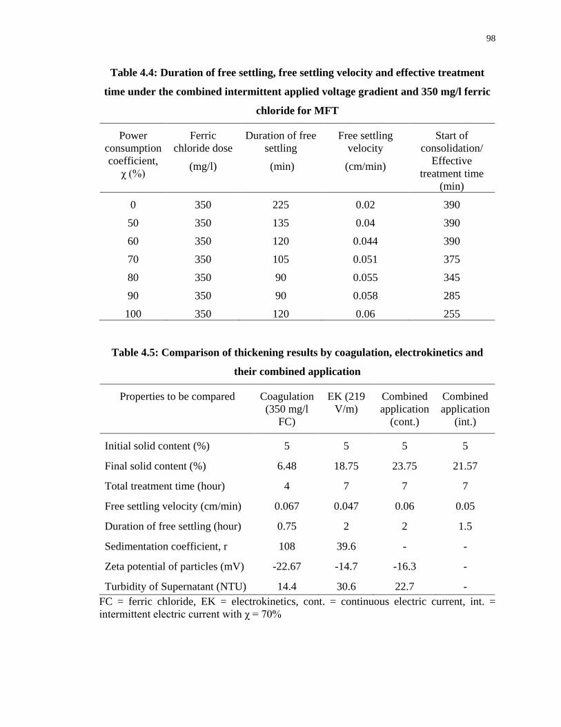
98
Table 4.4: Duration of free settling, free settling velocity and effective treatment
time under the combined intermittent applied voltage gradient and 350 mg/l ferric
chloride for MFT
Power consumption coefficient,
χ (%)
Ferric chloride dose
(mg/l)
Duration of free settling
(min)
Free settling velocity
(cm/min)
Start of consolidation/
Effective treatment time
(min)
0 350 225 0.02 390
50 350 135 0.04 390
60 350 120 0.044 390
70 350 105 0.051 375
80 350 90 0.055 345
90 350 90 0.058 285
100 350 120 0.06 255
Table 4.5: Comparison of thickening results by coagulation, electrokinetics and
their combined application
Properties to be compared Coagulation (350 mg/l
FC)
EK (219 V/m)
Combined application
(cont.)
Combined application
(int.)
Initial solid content (%) 5 5 5 5
Final solid content (%) 6.48 18.75 23.75 21.57
Total treatment time (hour) 4 7 7 7
Free settling velocity (cm/min) 0.067 0.047 0.06 0.05
Duration of free settling (hour) 0.75 2 2 1.5
Sedimentation coefficient, r 108 39.6 - -
Zeta potential of particles (mV) -22.67 -14.7 -16.3 -
Turbidity of Supernatant (NTU) 14.4 30.6 22.7 - FC = ferric chloride, EK = electrokinetics, cont. = continuous electric current, int. = intermittent electric current with χ = 70%
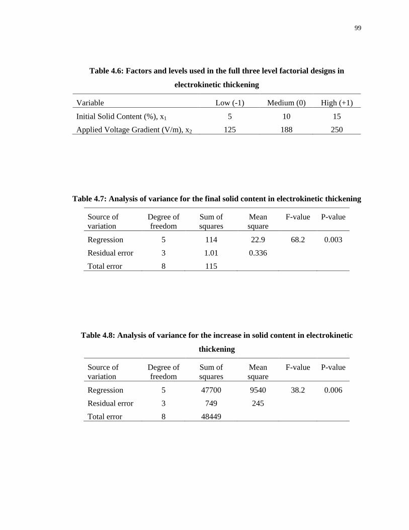
99
Table 4.6: Factors and levels used in the full three level factorial designs in
electrokinetic thickening
Variable Low (-1) Medium (0) High (+1)
Initial Solid Content (%), x1 5 10 15
Applied Voltage Gradient (V/m), x2 125 188 250
Table 4.7: Analysis of variance for the final solid content in electrokinetic thickening
Source of variation
Degree of freedom
Sum of squares
Mean square
F-value P-value
Regression 5 114 22.9 68.2 0.003
Residual error 3 1.01 0.336
Total error 8 115
Table 4.8: Analysis of variance for the increase in solid content in electrokinetic
thickening
Source of variation
Degree of freedom
Sum of squares
Mean square
F-value P-value
Regression 5 47700 9540 38.2 0.006
Residual error 3 749 245
Total error 8 48449
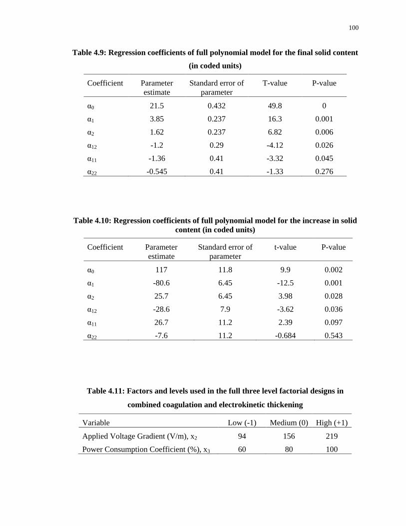
100
Table 4.9: Regression coefficients of full polynomial model for the final solid content (in coded units)
Coefficient Parameter estimate
Standard error of parameter
T-value P-value
α0 21.5 0.432 49.8 0
α1 3.85 0.237 16.3 0.001
α2 1.62 0.237 6.82 0.006
α12 -1.2 0.29 -4.12 0.026
α11 -1.36 0.41 -3.32 0.045
α22 -0.545 0.41 -1.33 0.276
Table 4.10: Regression coefficients of full polynomial model for the increase in solid content (in coded units)
Coefficient Parameter estimate
Standard error of parameter
t-value P-value
α0 117 11.8 9.9 0.002
α1 -80.6 6.45 -12.5 0.001
α2 25.7 6.45 3.98 0.028
α12 -28.6 7.9 -3.62 0.036
α11 26.7 11.2 2.39 0.097
α22 -7.6 11.2 -0.684 0.543
Table 4.11: Factors and levels used in the full three level factorial designs in
combined coagulation and electrokinetic thickening
Variable Low (-1) Medium (0) High (+1)
Applied Voltage Gradient (V/m), x2 94 156 219
Power Consumption Coefficient (%), x3 60 80 100
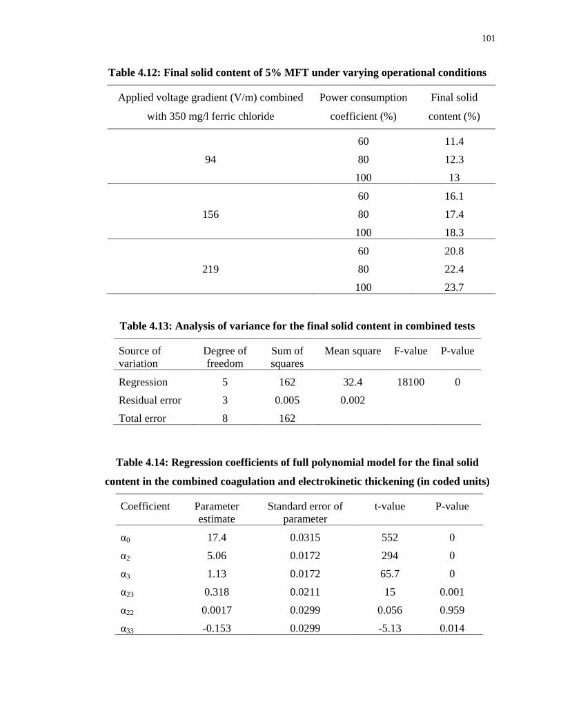
101
Table 4.12: Final solid content of 5% MFT under varying operational conditions
Applied voltage gradient (V/m) combined
with 350 mg/l ferric chloride
Power consumption
coefficient (%)
Final solid
content (%)
60 11.4
94 80 12.3
100 13
60 16.1
156 80 17.4
100 18.3
60 20.8
219 80 22.4
100 23.7
Table 4.13: Analysis of variance for the final solid content in combined tests
Source of variation
Degree of freedom
Sum of squares
Mean square F-value P-value
Regression 5 162 32.4 18100 0
Residual error 3 0.005 0.002
Total error 8 162
Table 4.14: Regression coefficients of full polynomial model for the final solid
content in the combined coagulation and electrokinetic thickening (in coded units)
Coefficient Parameter estimate
Standard error of parameter
t-value P-value
α0 17.4 0.0315 552 0
α2 5.06 0.0172 294 0
α3 1.13 0.0172 65.7 0
α23 0.318 0.0211 15 0.001
α22 0.0017 0.0299 0.056 0.959
α33 -0.153 0.0299 -5.13 0.014
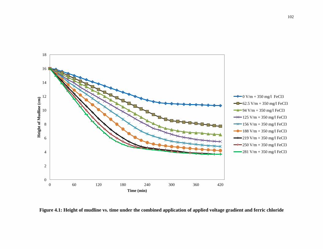
102
0
2
4
6
8
10
12
14
16
18
0 60 120 180 240 300 360 420
Hei
ght o
f Mud
line
(cm
)
Time (min)
0 V/m + 350 mg/l FeCl3
62.5 V/m + 350 mg/l FeCl3
94 V/m + 350 mg/l FeCl3
125 V/m + 350 mg/l FeCl3
156 V/m + 350 mg/l FeCl3
188 V/m + 350 mg/l FeCl3
219 V/m + 350 mg/l FeCl3
250 V/m + 350 mg/l FeCl3
281 V/m + 350 mg/l FeCl3
Figure 4.1: Height of mudline vs. time under the combined application of applied voltage gradient and ferric chloride

103
0
50
100
150
200
250
300
350
400
0
5
10
15
20
25
0 50 100 150 200 250 300
Incr
ease
in S
olid
Con
tent
(%)
Fina
l Sol
id C
onte
nt (%
)
Applied Voltage Gradient (V/m) combined with 350 mg/l Ferric Chloride
Final Solid Content Increase in Solid Content
Figure 4.2: Final solid content and increase in solid content vs. combined applied voltage gradient and 350 mg/l ferric chloride
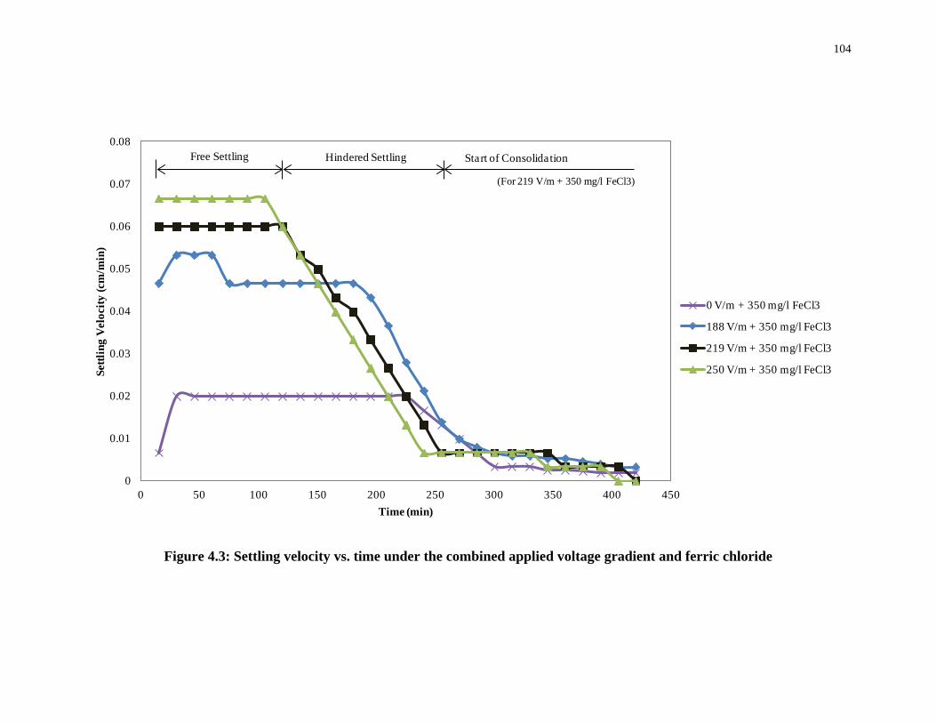
104
0
0.01
0.02
0.03
0.04
0.05
0.06
0.07
0.08
0 50 100 150 200 250 300 350 400 450
Settl
ing
Vel
ocity
(cm
/min
)
Time (min)
0 V/m + 350 mg/l FeCl3
188 V/m + 350 mg/l FeCl3
219 V/m + 350 mg/l FeCl3
250 V/m + 350 mg/l FeCl3
Free Settling Hindered Settling Start of Consolidation
(For 219 V/m + 350 mg/l FeCl3)
Figure 4.3: Settling velocity vs. time under the combined applied voltage gradient and ferric chloride

105
92
93
94
95
96
97
98
0
50
100
150
200
250
300
0 50 100 150 200 250 300
Vol
tage
Eff
icie
ny (%
)
Eff
ectiv
e V
olta
ge G
radi
ent b
etw
een
anod
e an
d ca
thod
e (V
/m)
Applied Voltage Gradient (V/m) combined with 350 mg/l Ferric Chloride
Effective Voltage Gradient Voltage Effiecieny
Figure 4.4: Effective voltage gradient and voltage efficiency between anode and
cathode vs. applied voltage gradient combined with ferric chloride
y = 8E-06x + 9E-06R² = 0.992
0
0.0005
0.001
0.0015
0.002
0.0025
0 50 100 150 200 250 300
Cur
rent
Den
sity
(A/m
2 )
Applied Volatge Gradient (V/m) combined with 350 mg/l Ferric Chloride
Figure 4.5: Current density vs. applied voltage gradient combined with ferric
chloride

106
0
1
2
3
4
5
6
7
0 50 100 150 200 250 300
Pow
er C
onsu
mpt
ion
(KW
/m3 )
Applied Voltage Gradient (V/m) combined with 350 mg/l FeCl3
Figure 4.6: Power consumption vs. applied voltage gradient combined with ferric
chloride
-35
-30
-25
-20
-15
-10
-50 50 100 150 200 250 300
Zeta
Pot
entia
l (m
V)
Applied Voltage Gradient (V/m) combined with 350 mg/l FeCl3
Figure 4.7: Final zeta potential of particles vs. applied voltage gradient under the
combined application of electrokinetics and coagulation
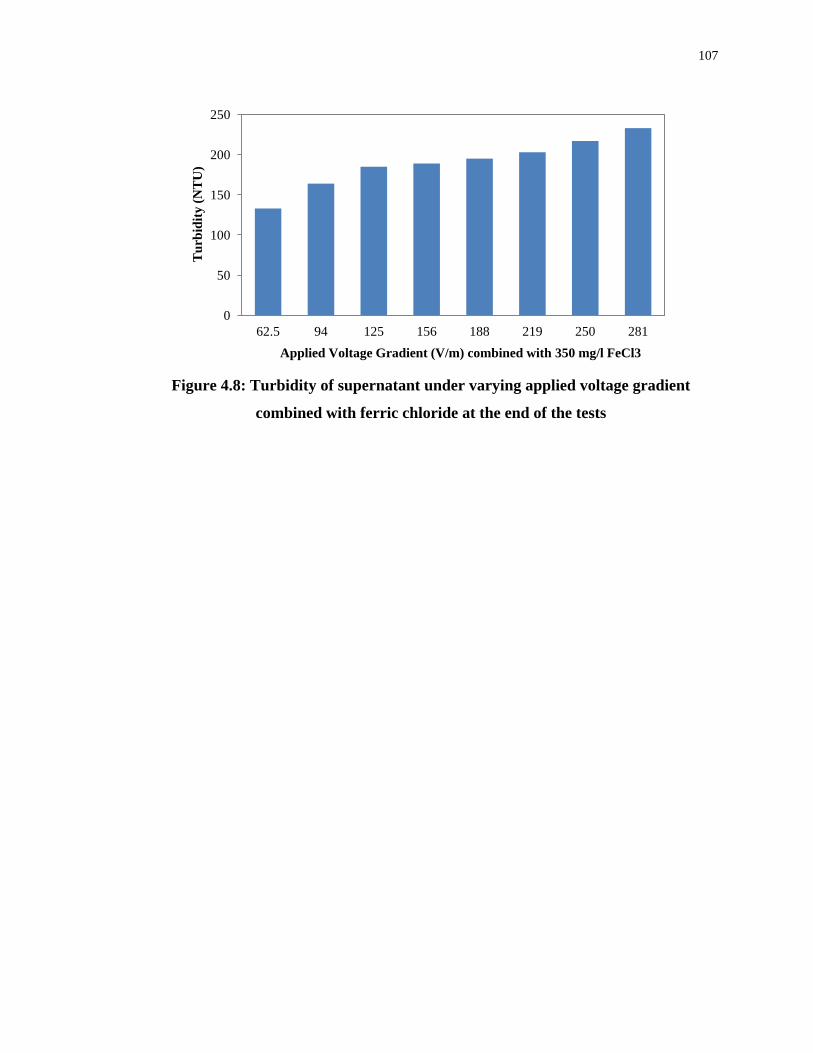
107
0
50
100
150
200
250
62.5 94 125 156 188 219 250 281
Tur
bidi
ty (N
TU
)
Applied Voltage Gradient (V/m) combined with 350 mg/l FeCl3
Figure 4.8: Turbidity of supernatant under varying applied voltage gradient
combined with ferric chloride at the end of the tests
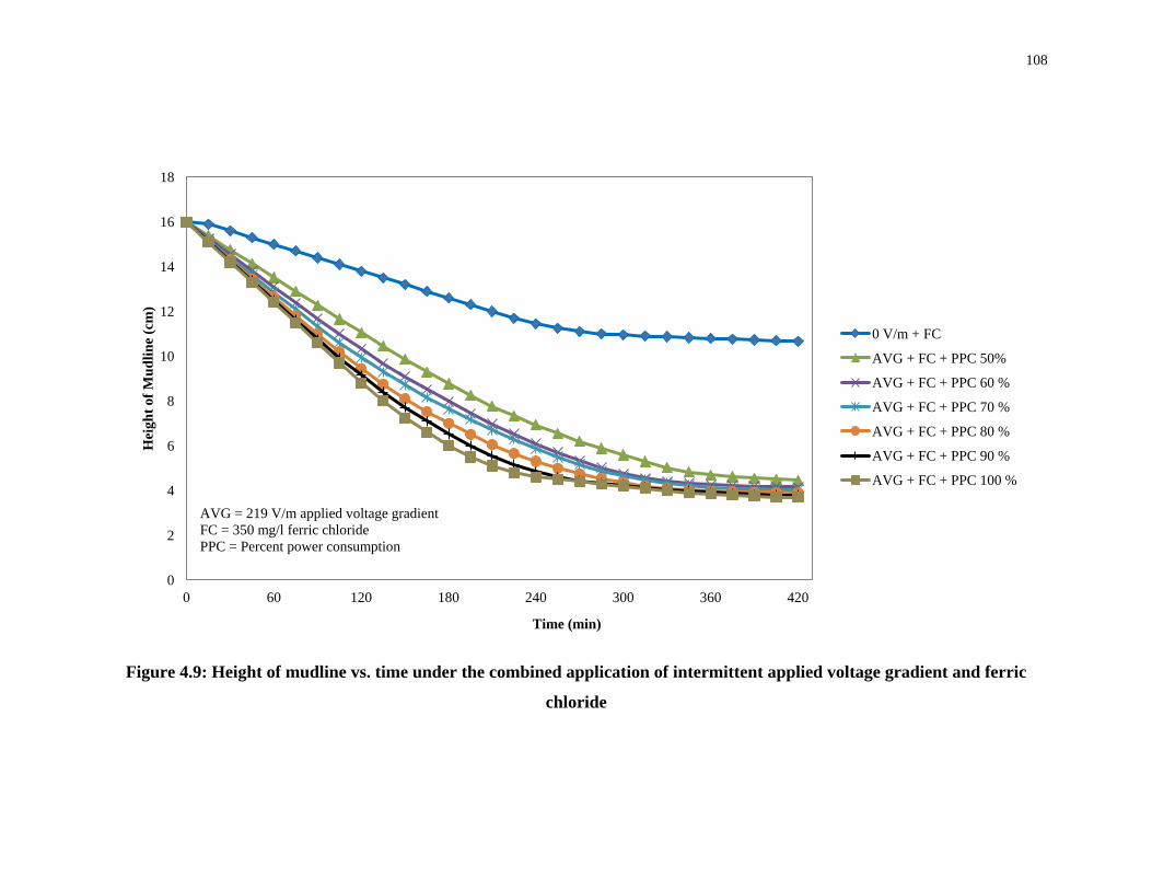
108
0
2
4
6
8
10
12
14
16
18
0 60 120 180 240 300 360 420
Hei
ght o
f Mud
line
(cm
)
Time (min)
0 V/m + FC
AVG + FC + PPC 50%
AVG + FC + PPC 60 %
AVG + FC + PPC 70 %
AVG + FC + PPC 80 %
AVG + FC + PPC 90 %
AVG + FC + PPC 100 %
AVG = 219 V/m applied voltage gradientFC = 350 mg/l ferric chloridePPC = Percent power consumption
Figure 4.9: Height of mudline vs. time under the combined application of intermittent applied voltage gradient and ferric
chloride
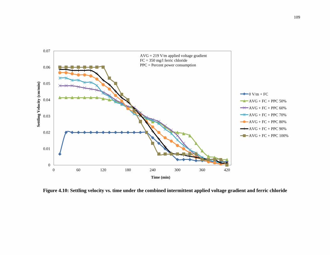
109
0
0.01
0.02
0.03
0.04
0.05
0.06
0.07
0 60 120 180 240 300 360 420
Sett
ling
Vel
ocity
(cm
/min
)
Time (min)
0 V/m + FC
AVG + FC + PPC 50%
AVG + FC + PPC 60%
AVG + FC + PPC 70%
AVG + FC + PPC 80%
AVG + FC + PPC 90%
AVG + FC + PPC 100%
AVG = 219 V/m applied voltage gradientFC = 350 mg/l ferric chloridePPC = Percent power consumption
Figure 4.10: Settling velocity vs. time under the combined intermittent applied voltage gradient and ferric chloride

110
0
50
100
150
200
250
300
350
400
0
5
10
15
20
25
0 20 40 60 80 100
Incr
ease
in S
olid
Con
tent
(%)
Fina
l Sol
id C
onte
nt (%
)
Power Consumption Coefficient, χ (%) combined with Ferric Chloride
Final Solid Content Increase in Solid Content
Figure 4.11: Final solid content and increase in solid content vs. power consumption coefficient under the combined
intermittent applied voltage gradient and 350 mg/l ferric chloride
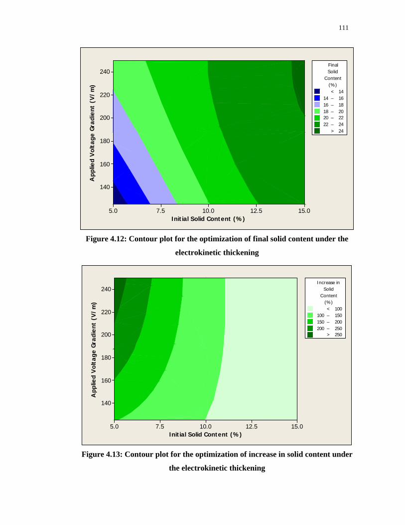
111
Initial Solid Content (%)
App
lied
Vol
tage
Gra
dien
t (V
/m)
15.012.510.07.55.0
240
220
200
180
160
140
> – – – – – < 14
14 1616 1818 2020 2222 24
24
(%)Content
SolidFinal
Figure 4.12: Contour plot for the optimization of final solid content under the
electrokinetic thickening
Initial Solid Content (%)
App
lied
Vol
tage
Gra
dien
t (V
/m)
15.012.510.07.55.0
240
220
200
180
160
140
> – – – < 100
100 150150 200200 250
250
(%)Content
SolidIncrease in
Figure 4.13: Contour plot for the optimization of increase in solid content under
the electrokinetic thickening
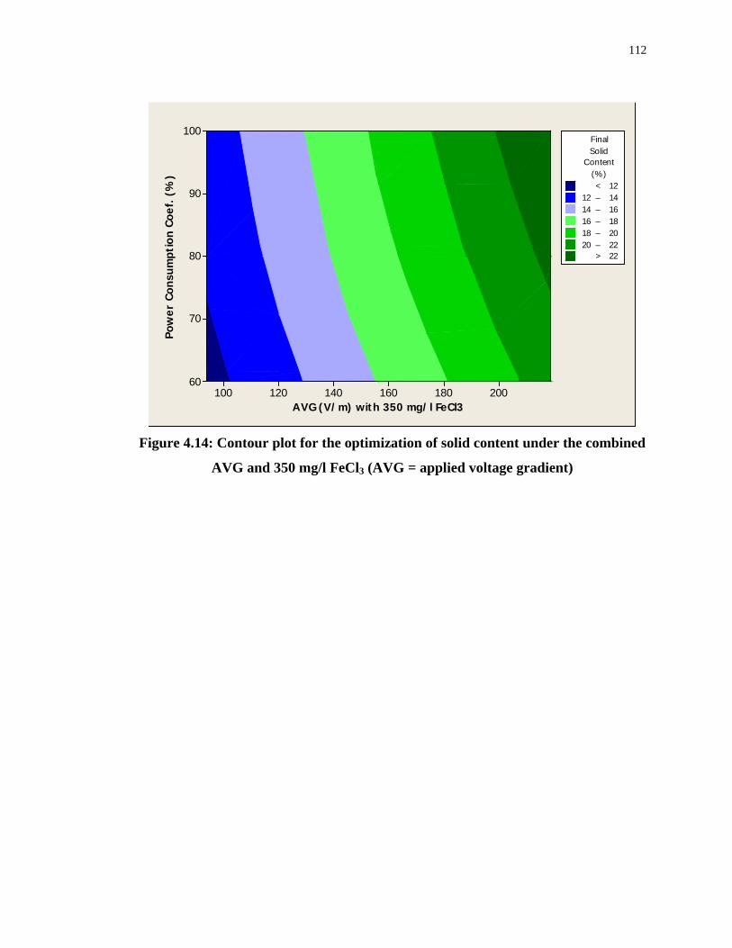
112
AVG (V/m) with 350 mg/l FeCl3
Pow
er C
onsu
mpt
ion
Coef
. (%
)
200180160140120100
100
90
80
70
60
> – – – – – < 12
12 1414 1616 1818 2020 22
22
(%)Content
SolidFinal
Figure 4.14: Contour plot for the optimization of solid content under the combined
AVG and 350 mg/l FeCl3 (AVG = applied voltage gradient)

113
CHAPTER 5 CONCLUSIONS AND RECOMMENDATIONS
5.1 Summary
A broad study on thickening of mature fine oil sands tailings by coagulation and
electrokinetics was conducted in this thesis. The geotechnical and mineralogical
properties of the solids and chemical properties of the pore water of MFT were
examined before the thickening tests on MFT suspensions. The study was divided
basically into two parts: (a) thickening of MFT suspensions by coagulation and
electrokinetics separately, and (b) combined application of coagulation and
electrokinetics to thicken the MFT suspensions. Coagulation tests were conducted into
jar apparatus to find out the optimum coagulant and coagulant dosage by observing the
location of mudline and final solid content of MFT. The coagulation tests in graduated
cylinder were carried out to thicken the MFT suspension and the results are examined in
terms of the mudline position, thickening velocity, final solid content of MFT and
turbidity of supernatant after settling. In electrokinetic thickening tests the most
effective initial solid content was determined first and then the final solid content of the
sediments, thickening velocity, power consumption, and turbidity of the supernatant
during and/or at the of the tests were measured on the MFT suspensions of 5% initial
solid content. The combined thickening tests contained two phases which are: (a) the
combined effect of the electric voltage gradient and 350 mg/l ferric chloride, and (b) the
combined effect of intermittent current in providing the threshold applied voltage
gradient of 219 V/m and 350 mg/l ferric chloride as coagulant.
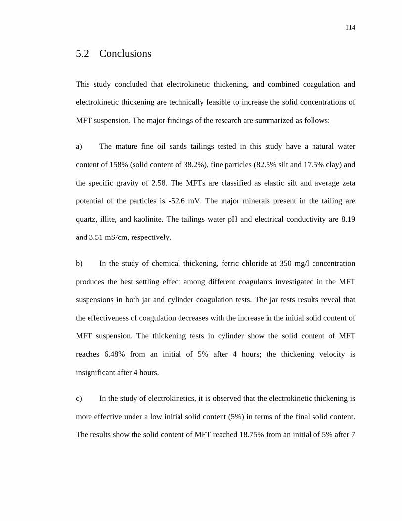
114
5.2 Conclusions
This study concluded that electrokinetic thickening, and combined coagulation and
electrokinetic thickening are technically feasible to increase the solid concentrations of
MFT suspension. The major findings of the research are summarized as follows:
a) The mature fine oil sands tailings tested in this study have a natural water
content of 158% (solid content of 38.2%), fine particles (82.5% silt and 17.5% clay) and
the specific gravity of 2.58. The MFTs are classified as elastic silt and average zeta
potential of the particles is -52.6 mV. The major minerals present in the tailing are
quartz, illite, and kaolinite. The tailings water pH and electrical conductivity are 8.19
and 3.51 mS/cm, respectively.
b) In the study of chemical thickening, ferric chloride at 350 mg/l concentration
produces the best settling effect among different coagulants investigated in the MFT
suspensions in both jar and cylinder coagulation tests. The jar tests results reveal that
the effectiveness of coagulation decreases with the increase in the initial solid content of
MFT suspension. The thickening tests in cylinder show the solid content of MFT
reaches 6.48% from an initial of 5% after 4 hours; the thickening velocity is
insignificant after 4 hours.
c) In the study of electrokinetics, it is observed that the electrokinetic thickening is
more effective under a low initial solid content (5%) in terms of the final solid content.
The results show the solid content of MFT reached 18.75% from an initial of 5% after 7

115
hours treatment under the applied voltage gradient of 219 V/m, which is significantly
better than the chemical coagulation.
d) The theory of sedimentation velocity in the free settling and hindered settling
stages was validated using the results of this research.
e) The final solid content of MFT after 7 hours of thickening is 23.74% from the
initial of 5% under the voltage gradient of 219 V/m and 350 mg/l ferric chloride, further
enhances thickening results. The intermittent application of electric current decreases
the final solid content of MFT compared to the treatment with continuous electric
current.
f) Under the optimized treatment of combined application, the zeta potential of the
tailings particles after the thickening test is the lowest in all treatments, including
coagulation, electrokinetics, and combined application. The corresponding turbidity of
the supernatant is 14.4 NTU, 30.6 NTU, and 22.7 NTU after 1 hour from the end of the
tests.
g) The developed regression models for electrokinetic thickening and combined
application of coagulation and electrokinetic thickening fit well with the experimental
data and statistically significant.

116
5.3 Recommendations for Future Research Work
The results of this research reveal that coagulant assisted electrokinetic thickening of
mature fine oil sands tailings is effective. With knowledge gained from this research, a
number of recommendations could be made for future studies:
• In this study the vertical distance between electrodes was constant and voltage
gradient was varied by changing the applied voltage. The vertical distance should be a
key variable in further study. The vertical distance may also be changed by using
movable cathode.
• The viscosity of tailings water may have strong effect on thickening of oil sands
tailings. It is recommended to examine the efficiency of electrokinetic thickening by
reducing the viscosity of water at higher temperature.
• The opening (aperture size) of electrodes should be optimized in future study to
thicken MFT suspension.
• The property of MFT solids might be changed due to electrochemical reaction at
anode. So the tailings solids property should be analyzed whether it meet the
regulatory standards for dumping.
• A field scale tests on thickening of MFT should be developed to further
investigate the effects of combined coagulation and electrokinetic thickening,
including the development of a detailed field scale implementation scheme.

117
• The current study did not focus on the technical issues and so cost-benefit
analysis of this technology should be carried out to provide more practical information
to the owner.
118
BIBLIOGRAPHY
Alam, R., Shang, J.Q., and Islam, S. (2014). Electrokinetic sedimentation of mature oil
sands mine tailings. 67th Canadian Geotechnical Conference, Regina,
Saskatchewan.
Amokrane, A., Comel, C., and Veron, J. (1997). Landfill leachates pre-treatment by
coagulation flocculation. Water Research, Vol. 31, No. 11, pp. 2775-2782.
Baghvand, A., Zand, A.D., Mehrdadi, N., and Karbassi, A. (2010). Optimizing
coagulation process for low to high turbidity waters using aluminum and iron
salts. American Journal of Environmental Sciences, Vol. 6, No. 5, pp. 442-448.
Beier, N., and Sego, D. (2008). The oil sands tailings research facility. Geointerest,
Geotechnical News.
BGC Engineering Inc. (2010). Oil sands tailings technology review. Oil Sands Research
and Information Network, University of Alberta, School of Energy and the
Environment, Edmonton, Alberta, OSRIN Report No. TR-1.
Box, G.E.P., and Draper, N.R. (1987). Empirical model-building and response surface,
Wiley, New York.
Buckland, D.G., Shang, J.Q., and Mohamedelhassan, E. (2000). Electrokinetic
sedimentation of contaminated Welland river sediment. Canadian Geotechnical
Journal, Vol. 37, pp. 735-747.
119
Camenen, B., and Bang, D.P.V. (2011). Modelling the settling of suspended sediments
for concentrations close to the gelling concentration. Continental Shelf
Research, Vol. 31, No. 10, pp. 106 -111.
Cabrera, S.C.M., Bryan, J., Komishke, B., and Kantzas, A. (2009). Study of the settling
characteristics of tailings using nuclear magnetic resonance technique.
International Journal of Mining, Reclamation and Environment, Vol. 23, No. 1,
pp. 33–50.
Caughill, D.L., Morgenstern, N.R., and Scott, J.D. (1993). Geotechnics of
nonsegregating oil sands tailings. Canadian Geotechnical Journal, Vol. 30, No.
5, pp. 801-811.
Chalaturnyk, R.J., Scott, J.D., and Ozum, B. (2002). Management of oil sands tailings.
Petroleum Science & Technology, Vol. 20, No.9, pp. 1025.
Concha, F., and Burger, R. (2003). Thickening in the 20th Century: a historical
perspective. Mineral & Metallurgical Processing, Vol. 20, pp. 57- 67.
Dankers, P., and Winterwerp, J. (2007). Hindered settling of mud flocs: theory and
validation. Continental Shelf Research, Vol. 27, pp. 1893-1907.
Dawson, R.F. and Sego, D.C. (1993). Design concepts for thin layered freeze-thaw
dewatering systems. Proceedings of the 46th Canadian Geotechnical Conference,
Saskatoon, pp. 283-288.
Fair, A. (2008). The Past, Present and Future of Tailings at Syncrude. International Oil
Sands Tailings Conference, Edmonton, Alberta.
120
FTFC- Fine Tailings Fundamentals Consortium. (1995). Advances in Oil Sands
Tailings Research, Alberta Department of Energy, Oil Sands and Research
Division, Alberta.
Genovese, C.V., and Gonzalez, J. F. (1998). Solids Removal by Coagulation from
Fisheries Wastewaters, Water SA, Vol. 24, No. 4, pp. 371-372.
Gladman, B.J., Usher, S.P., and Scales, P.J. (2006). Understanding the thickening
process. IN: Jewell, R.J., Lawson, S., and Newman, P. (eds), Paste- 2006,
Australian Centre for Geomechanics, Perth.
Government of Alberta. (2010). Alberta's Oil Sands. Fact Sheets - Tailings management.
Government of Alberta, Edmonton, Alberta.
Guo, Y., and Shang, J.Q. (2014). A study on electrokinetic dewatering of oil sands
tailings. Environmental Geotechnics, Vol. 1, No. EG2, pp 121-134.
Houlihan, R. and Haneef, M. (2008). Oil Sands Tailings: Regulatory Perspective.
International Oil Sands Tailing Conference, Edmonton, Alberta.
Jaikumar, V., and Ramamurthi, V. (2009). Statistical analysis and optimization of acid
dye biosorption by brewery waste biomass using response surface methodology.
Modern Applied Science, Vol. 3, No. 4, pp 71-84.
Jeeravipoolvarn, S. (2010). Geotechnical behaviour of in-line thickened oil sands
tailings. PhD thesis, University of Alberta, Edmonton, Alberta.
Jewell, R.J., and Fourie, A.B. (2006). Paste and Thickened tailings- a guide. 2nd ed.,
Australian Centre for Geomechanics, The University of Western Australia,
Nedlands, Western Australia.
121
Kasperski, K.L. (1992). A review of properties and treatment of oil sands tailings.
AOSTRA Journal of Research, Vol. 8, pp. 11-53.
Kim, S.S., Lee, M., and Kim, D.H. (2008). Electrokinetic settling and sedimentation
behavior of cohesive soils in dilute suspension. Journal of Environmental
Science and Health, Vol. 43 (Part A), pp. 975-984.
Kynch, G.J. (1952). A theory of sedimentation, Trans. Faraday Soc., Vol. 48, pp. 166-
167.
Lockhart, N.C. (1983a). Electro-osmotic dewatering of clays, II. Influence of salts,
acids and flocculants. Colloids and Surface, Vol. 6, No. 3, pp. 239-251.
Lockhart, N.C. (1983b). Electro-osmotic dewatering of clays, III. Influence of clay
types, exchangeable cations and electrode materials. Colloids and Surface, Vol.
6, No. 3, pp. 253-269.
Lockhart, N.C., and Stickland, R.E. (1984). Dewatering coal washery tailings ponds by
electroosmosis. Powder Technology, Vol. 40, pp. 215-221.
Lockhart, N.C. (1986). Electro-dewatering of fine suspensions. In: Muralidhra, H.S.
(ed), Advances in solid-liquid separation, Battelle Press, Columbus, Ohio, pp.
241-274.
Lo, K.Y., and Shang, J.Q. 1995. Applications of electrokinetics in mine reclamation.
Proceedings of the 1st SCH-CORE Workshop, Beijing, China.
Malakootian, M., and Fatehizadeh, A. (2010). Color removal from water by
coagulation/ caustic soda and lime. Iranian Journal of Environmental Health
Science and Engineering, Volume 7. No. 3, pp. 267-272.
122
McRoberts, E.C., and Nixon, J.F. (1976). A theory of soi1 sedimentation. Canadian
Geotechnical Journal, Vol. 13, pp. 294-3 10.
Mikula, R.J., Munoz, V.A., and Omotosa, O. (2009). Centrifuge options for production
of dry stakeable tailings in surface mined oil sands tailings management. Journal
of Canadian Petroleum Technology, Vol. 48, No. 9, pp. 19-23.
Mitchell, J.K. (1993). Fundamentals of soil behaviour, 2nd ed., John Wiley and Sons,
New York.
Mohamedelhassan, E. (2008). Electrokinetic sedimentation and dewatering of clay
slurries. Proceedings of the First International Conference on Oil Sands Tailings,
Edmonton, Canada, December 2008, pp. 153-160.
Mohamedelhassan, E., and Shang, J.Q. (2001). Effects of electrode materials and
current intermittence in electroosmosis. Ground Improvement, Vol.5, No.1, pp.
3-11.
Montgomery, D.C. (2001). Design and analysis of experiments. 5th ed., John Wiley and
Sons, New York, USA.
Pourrezaei, P., and El-Din, M.G. (2008). Coagulation-flocculation pre-treatment of oil
sands process affected water. 1st International oil sands tailings conference
(IOSTC), Edmonton, Alberta, Canada.
Rabie, H.R., Munjumder, A. S., and Webberss, M.E. (1994). Interrupted electro-
osmotic dewatering of clay suspensions. Separations Technology, Vol. 4, pp.
38-46.

123
Richardson, V.F., and Zaki, W.N. (1954). Sedimentation and fluidization, Part 1, Tnans.
Int. Chem. Eng., Vol. 32, pp. 35-53.
Russel, W.B., Saville, D.A., and Schowalter, W.R. (1989). Colloidal dispersions,
Cambridge University Press, Cambridge, UK.
Scott, J.D., Dusseault, M.B., and Carrier III, W.D. (1985). Behavior of the clay/
bitumen/ water sludge system from oil sands extraction plants. Applied Cllay
Science, Vol. 1, pp. 207-218.
Scott, J.D., Jeeravipoolvarn, S., Donahue, R., and Ozum, B. (2008). Characterization of
oil sands thickened tailings. International Oil Sands Tailings Conference,
Geotechnical Centre, University of Alberta, Canada.
Shang, J.Q. (1997). Electrokinetic sedimentation: a theoretical and experimental study.
Canadian Geotechnical Journal, Vol. 34, No. 2, pp. 305-314.
Shang, J.Q., and Lo, K.Y. (1997). Electrokinetic dewatering of a phosphate clay.
Journal of Hazardous Material, Vol. 55, pp. 117-133.
Shen, Y.H. (2005). Treatment of low turbidity water by sweep coagulation using
bentonite. J. Chem. Technol. Biot., Vol. 80, pp. 581-586.
Silva, M.J. (1999). Plant dewatering and strengthening of mine waste tailings. PhD
thesis, University of Alberta, Edmonton, Alberta.
Soulsby, R. (1997). Dynamics of marine sands, a manual for practical applications.
Thomas Telford, London, UK, ISBN 0-7277-2584X.
Sowers, G.F. (1979). Introductory soil mechanics and foundations: Geotechnical
engineering, 4th ed., Macmillan, New York.

124
Sprute, R.H., and Kelsh, D.J. (1980). Dewatering fine particle suspensions with direct
current. Proceedings of International Symposium on Fine Particle Processes,
Vol. 2, Las Vegas, Nevada, pp. 1828-1844.
Stanczyk, M.H., and Feld, I.L. (1964). Electro-dewatering tests of Florida phosphate
rock slime. Vol. 6451 of Report of Investigations, Department of the Interior,
U.S. Bureau of Mines, pp. 1-19.
Svarovsky, L. (1990). Solid-liquid separationion, 3rd ed., Butterworth-Heihnemann Ltd.,
London.
Suncor (2010). Report on sustainability, Suncor energy, Suncor Inc.
(http://sustainability.suncor.com/2010/en/responsible/1779.aspx)
Wang, X., Feng, X., Xu, Z., and Masliyah, J.H. (2010). Polymer aids in settling and
filtration of oil sands tailings. The Canadian Journal of Chemical Engineering.
Vol. 88, No. 3, pp. 403-410.
Xu, Y., Dabros, T., and Kan, J. (2008). Filterability of oil sands tailings. Process Safety
and Environmental Protection, Vol. 86, No. 4, pp. 268-276.
Yukselen, M.A., and Gregory, J. (2004). The effect of rapid mixing on the break-up and
re-formation of flocs. J. Chem. Technol. Biot., Vol. 79, pp. 782-788.
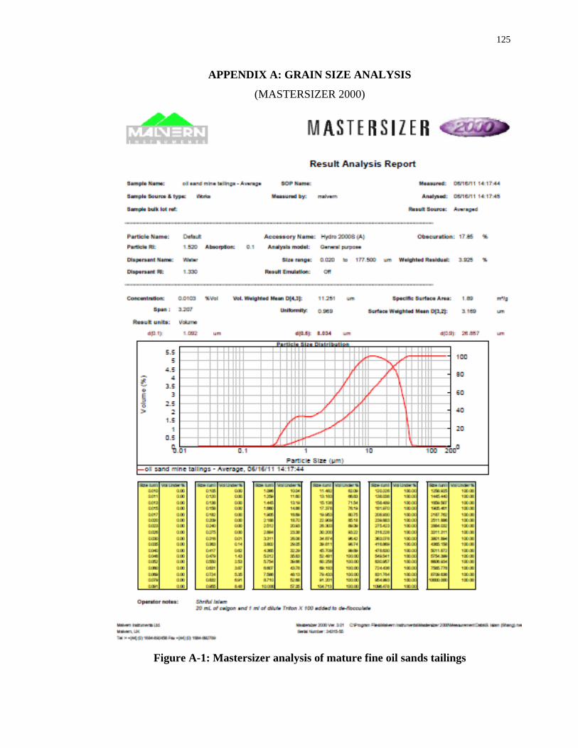
125
APPENDIX A: GRAIN SIZE ANALYSIS
(MASTERSIZER 2000)
Figure A-1: Mastersizer analysis of mature fine oil sands tailings
126
CURRICULUM VITAE
Name: Shriful Islam
Education: 2011-2014 M.E.Sc.
Department of Civil and Environmental Engineering
Western University, London, Ontario, Canada
2003-2009 B.Sc. Eng.
Department of Civil and Environmental Engineering
Shahjalal University of Science and Technology, Sylhet,
Bangladesh
Honours and
Awards:
2012
The R.M. Quigey Award
Geotechnical Research Centre (GRC)
2004-2008
University Scholarship
Shahjalal University of Science and Technology
1998-1999
Junior School Scholarship
Education Board, Bangladesh
Related Work
Experience
2011-2012, 2014-2014
Research Assistant
Department of Civil and Environmental Engineering
Western University, London, ON
2011-2012, 2014-2014
Teaching Assistant
Department of Civil and Environmental Engineering
Western University, London, ON

127
2013 - to date
Lecturer, Department of Civil and Environmental Engineering
Shahjalal University of Science and Technology, Bangladesh
2009-2011
Lecturer, Department of Civil Engineering
Int. University of Buss Agri and Tech., Bangladesh.
Selected
Publications:
Alam, R., Shang, J.Q., and Islam, S. (2014). Electrokinetic
Sedimentation of Mature Oil Sand Mine Tailings. GEO Regina
2014- 67th Canadian Geotechnical Conference, Regina,
Saskatchewan, Sep 28 – Oct 01, 2014.
S. Islam, and Shang, J.Q. Electrokinetic Thickening of Mature
Fine Oil Sands Tailing. (Under Preparation)
Islam, M.A., Rahman, M.S., Islam, S., Zakaria, A.N.M. and
Islam, K.M.R. (2012). A study on Arsenic Uptaking Capacity of
Water Hyacinth, Asian Journal of Water Environment and
Pollution, Vol. 9, No. 1, pp. 25-29.
Islam, S., Rasul, M.T., Alam, M.J.B., and Haque. M.A. (2011).
Evaluation of Water Quality of the Titas River Using NSF Water
Quality Index, Journal of Scientific Research, Vol. 3, No. 1, pp.
151-159.