The Structure of Political Choices: DistinguishingBetween Constraint and Multidimensionality*

William Marble† Matthew Tyler‡

June 18, 2018Click here for most recent version.

Abstract

In the literatures on public opinion and legislative behavior, there are debates overboth how constrained preferences are and whether they are best summarized on asingle left-right spectrum or are multidimensional. However, insufficient formalizationhas led to conflation between lack of constraint and multidimensionality. In this paper,we clarify these concepts in a formal framework, highlighting that they play differentroles in making political choices. We use this discussion to motivate cross-validationestimators that measure constraint and dimensionality in the context of canonical idealpoint models. Using data from the public and politicians, we find that American politi-cal preferences are homogeneously unidimensional, but there is more constraint amongpoliticians than the mass public. Further, we show that differences between politiciansand the public cannot be attributed to differences in agendas or the incentives faced bythe actors.

Word Count: 8,520

*For helpful discussions and comments, we thank Adam Bonica, David Broockman, Justin Grimmer, AndyHall, and Jonathan Rodden. We also thank AdamBonica for sharing NPAT data. We are grateful to participantsat the Political Economy Breakfast and theWorkshop for Empirical American Politics at Stanford. An R packagefor implementing the MultiScale algorithm is available at https://github.com/matthewtyler/MultiScale.

†Ph.D. Candidate, Department of Political Science, Stanford University. wpmarble@stanford.edu‡Ph.D. Candidate, Department of Political Science, Stanford University. mdtyler@stanford.edu

Ideological scaling methods have long been a mainstay in legislative studies, and schol-

ars are increasingly applying these methods to disparate sources of data beyond roll-call

votes. The goal is to extract a simple, low-dimensional summary measure of ideology from

votes, survey responses, or other types of political data.¹ Typically, researchers seek to align

political actors on a simple left-right political spectrum, which can be used to characterize

public opinion and to study representation. Despite the prevalence of ideological scaling

methods, there remain unresolved debates about how to interpret the resulting estimates

— especially when applied to non-institutional actors such as survey respondents.

First, there is debate over the dimensionality of political conflict. In the study of

American politics, the default setting is to estimate a one-dimensional model, in line with

conventional wisdom about the dimensionality of Congress (cf. Poole and Rosenthal, 1997).

However, some researchers suggest as many as eight dimensions are needed to explain

Congressional voting patterns (Heckman and Snyder, 1997), and recent empirical work has

emphasized the importance of including more dimensions in ideal point estimates for the

public (Ansolabehere, Rodden and Snyder, 2008; Treier and Hillygus, 2009).

Second, there is debate over how constrained attitudes are in the public, which deter-

mines the interpretability of ideal point estimates. Some authors claim that most citizens

do not have well-formed political opinions, let alone opinions that can be meaningfully

described by a low-dimensional summary (e.g., Converse, 1964; Campbell et al., 1960; Kuk-

linski and Quirk, 2000; Kinder, 2003). In an extreme view, policy attitudes are unstable and

entirely idiosyncratic, meaning that scaling methods have little hope of recovering a useful

estimate of ideology. A slightly weaker formulation is that citizen preferences are somewhat

constrained, but that they are not amenable to a low-dimensional summary (Broockman,

2016; Lauderdale, Hanretty and Vivyan, 2017). In this case, only a small portion of variance

¹Foundational work in scaling roll-call votes includes Poole and Rosenthal (1997), Clinton, Jackman andRivers (2004), and Heckman and Snyder (1997). More recent studies applying similar methods to surveyresponses include Tausanovitch and Warshaw (2013), Pan and Xu (2018), and Jessee (2009). Bonica (2013)extends these methods to campaign finance data, while Barberá (2015) and Bond and Messing (2015) applythem to social media data.

1

in survey responses can be explained by a single dimension.

A common sentiment is that public opinion is multidimensional, while political conflict

among the parties is unidimensional. A natural implication is that a higher-dimensional

model should better describe public opinion data. Under this view, low constraint and

multidimensionality are synonyms.

In this paper, we seek to distinguish between these two notions, dimensionality and

constraint, in the context of ideal point models. Briefly, dimensionality refers to the number

of distinct (spatial) issues that are commonly understood and acted upon by all voters. In the

language of Heckman and Snyder (1997), the dimensionality is the number of “attributes”

of policy choices that are needed to rationalize votes. Constraint, in contrast, refers to how

much political actors rely on these attributes in forming opinions on particular policies. In

a highly constrained population of actors, knowing an actors’ opinions on one set of issues

should enable accurate prediction of further opinions, relative to an appropriately chosen

null model. In an unconstrained population, most policy attitudes are idiosyncratic and

unrelated to each other.

From this perspective, constraint and dimensionality are orthogonal concepts. Theoret-

ically, any population can exhibit any level of constraint with any level of dimensionality.

Whether any given population has low constraint while being multidimensional is an em-

pirical question.

Drawing on this theoretical discussion, we propose an out-of-sample model validation

procedure for ideal point models that enables us to estimate the dimensionality of political

choices and the associated level of constraint. In contrast, extant model validation efforts

in the literature have focused on in-sample fit or ad-hoc measures of out-of-sample fit.

We document evidence of significant overfitting in ideal point models, illustrating the

importance of a theoretically motivated out-of-sample validation strategy.

Using newly developed software, we apply the validation procedure to the workhorse

2

quadratic-utility ideal point model commonly used to estimate ideal points.² With an array

of data sets that encompass both politicians and the public, we draw three main empirical

conclusions.

First, we investigate claims in the literature that the structure of political conflict is best

characterized using higher-dimensional models. We find no evidence that multidimensional

models of ideal points explain preferences better than unidimensional models — in fact,

due to overfitting, higher dimensional models can perform worse than a model that does

not estimate ideal points at all. Second, we find that ideal point models are considerably

less powerful when applied to the public. In contrast with politicians, voter responses

are dominated by idiosyncratic, rather than ideological, preferences. This suggests the

public has low constraint, relative to politicians. Third, we decompose this difference in

model performance between the public and politicians. We find that nearly all of the

divergence can be attributed to differences in the constraint of the actors, rather than

different measurement tools or disparate incentives faced by the actors. When applied to

high-quality survey data of politicians, scaling methods perform nearly as well as when

applied to roll-call votes. We also take advantage of paired data sources of politicians and

the public to show that this conclusion is not driven by differences in the agenda or survey

design.

These results suggest caution in applying ideal point estimation methods to surveys in

the mass public. The resulting estimates do indeed explain some of the variation in stated

preferences. However, the variance in preferences for particular policies that is explained

by ideal points is considerably lower than for politicians. Idiosyncratic preferences —

rather than spatial preferences — tend to dominate voter attitudes. These results suggest

that scholars should employ measures of both spatial and idiosyncratic preferences when

studying political attitudes in the mass public.

²The software, called MultiScale and described in more detail below, enables fast estimation ofhigh-dimensional ideal point models with substantial amounts of missing data in R, enabling us to quicklyre-estimate ideal point models hundreds of times. It is available for download athttps://github.com/matthewtyler/MultiScale.

3

The rest of the paper is structured as follows. First, we describe the differences between

dimensionality and constraint and derive empirical implications. Then, we propose out-

of-sample validation procedures to measure them. Next, we address the debate about the

dimensionality of political conflict. Finally, we examine differences in constraint across pop-

ulations and contexts, while addressing possible explanations for the divergence between

elites and the mass public.

1 Multidimensionality and Constraint in a Theory of Choices

At least as far back as Campbell et al. (1960) and Converse (1964), scholars of public opinion

have been aware of the fact that American voters do not fit as cleanly inside ideological lines

as, say, members of Congress or state legislators. A common sentiment in this literature is

that voters’ policy attitudes are not derived from a coherent ideological framework. Instead,

attitudes are idiosyncratic or at least not structured in the same way as politicians’. This

perspective emphasizes a notion of ideology as constraint. Constraint here refers to the

degree to which policy attitudes on some issues are predictive of policy attitudes on other

issues. For example, if there is high degree of ideological constraint in the population, then

knowing a voter’s preferences for welfare spending should allow one to infer her preferred

tax rate. If there is a low degree of constraint, then knowing the voter’s preference about

the welfare spending tells us little about her preferred tax rate.

The primary evidence for the lack of constraint comes from the low inter-item correla-

tions between survey responses (Converse, 1964; Achen, 1975) and lack of knowledge about

which issues “go together” (Freeder, Lenz and Turney, Forthcoming). Summarizing one

view, Kinder (2003, 16) writes that “Converse’s original claim of ideological naïveté stands

up quite well, both to detailed reanalysis and to political change.”

This view implies that a unidimensional spatial model, as conceptualized by Downs

(1957) and others, is simply not useful for understanding public opinion. In contrast,

4

some scholars have attempted to salvage the idea of constrained voters by arguing that

a multidimensional model provides a more reasonable picture of how voters perceive pol-

itics (Marcus, Tabb and Sullivan, 1974). For example, Treier and Hillygus (2009) write

that “Our analysis documents the multidimensional nature of policy preferences in the

American electorate. . . [F]ailing to account for the multidimensional nature of ideological

preferences can produce inaccurate predictions of voting behavior.” Similarly, Barber and

Pope (2016) argue, “Voter attitudes should be seen as complex (multi-dimensional), in con-

trast with elites where similar measures indicate a much simpler (unidimensional) space

that describes virtually all of their attitudes.” In many of these arguments, the additional

dimensions are considered to be just as important as the first. For instance, Lauderdale,

Hanretty and Vivyan (2017) claim that including a second dimension nearly doubles how

much variance in stated preferences is attributable to ideology.³ An implied sentiment

is that observed levels of constraint increase with a more flexible notion of ideology that

encompasses multiple dimensions.

The goal of this paper is to distinguish between these two notions, constraint and

multidimensionality, and to provide rigorous measures of them. The dimensionality of

policy attitudes refers to the number of distinct underlying issues that are common to

all people responding to the survey (or voting on roll-call votes). For example, we may

think of policies as occupying a space with both “economic” and “moral” issue dimensions

that are understood in the same way by all political actors. Multidimensionality simply

refers to the presence of multiple such issues. The level of constraint, in contrast, refers to

how much knowledge of someone’s policy attitudes on some issues helps us predict their

policy attitudes on other issues through the common policy space. There may be many

idiosyncratic factors affecting individuals’ policy attitudes that have nothing to do with the

common policy space. The level of constraint refers to how much variance the common

³The stated predictive power of multiple dimensions varies greatly from study to study. For instance,Ansolabehere, Rodden and Snyder (2006) posit the existence of both an economic and a moral dimension,but downplay the importance of the moral dimension for explaining vote choice.

5

policy space explains relative to the idiosyncratic components.

There are no trade-offs between constraint and multidimensionality: either can appear

with or without the other. Whether or not voters are multidimensional has little to do with

whether or not they are more or less constrained. A natural implication of this discussion is

that there is a limit to how well we can predict political attitudes from other attitudes, since

modeling additional dimensions of ideology has diminishing (and, as we later document,

negative) returns.

1.1 Formalizing Constraint and Multidimensionality

The goal of this section is to make our ideas of constraint and multidimensionality concrete

in the context of canonical ideal point models. This formalization will allow us to derive

explicit observable implications, which we can use to empirically identify the presence or

lack of constraint and multidimensionality with data on political choices.

Many readers will be familiar with the quadratic utility spatial voting model used

in Clinton, Jackman and Rivers (2004, hereafter CJR); we couch our discussion in this

framework.⁴ Specifically, we will suppose the political actors we are studying — whether

they be members of Congress, survey respondents, etc. — have an ideal policy γi located

in some common Euclidean space. When considering two policy proposals, a yea policy

located at point ζj and a nay policy located at ψj , we model the actor as having a quadratic

utility function. With a slight abuse of notation, we formally write the utilities,

Ui (ζj ) = −||γi − ζj | |2 + ηi j (1)

Ui (ψj ) = −||γi − ψj | |2 + νi j, (2)

where Ui (·) denotes the utility of actor i under the specific policy proposal, | | · | |2 denotes

⁴In this article, we are agnostic as to whether or not the assumptions behind the CJR model are “correct” orcan be interpreted as structural. For our purposes, it is enough that the models predict or describe behavior.So, for instance, we are interested in these models even if the ideal points being measured are actually somereduced form combination of ideological, partisan, and constituent incentives.

6

the squared Euclidean distance (i.e., | |a | |2 = a′a), and ηi j and νi j are idiosyncratic com-

ponents not explained by Euclidean distance from the ideal policy γi . These idiosyncratic

components are treated as unobserved random variables. This utility specification makes

precise the various incentives the actor is facing: the spatial component of the utility func-

tion is meant to capture the idea that the actor prefers certain kinds of policy locations in

the common policy space over others (e.g., conservative policies), while the idiosyncratic

components capture the actor’s preferences that don’t fit neatly into the common policy

space (e.g., region-specific priorities).

It is convenient to denote the voter surplus (utility difference) of the yea policy proposal

over the nay policy proposal as si j = Ui (ζj )−Ui (ψj ). Actor i chooses the yea policy instead of

the nay policy if and only if the surplus for the policy is positive: si j > 0. We store the votes

of N actors on J pairs of policy proposals in the binary matrix Y , where yi j = I (si j > 0).

If we assume that the differences in idiosyncratic terms ηi j − νi j follow independent

mean zero normal distributions with variance σ2, then CJR show that the probability

of a yea vote, yi j = 1, is equal to Φ(αj + β′jγi ), where Φ(·) is the standard normal cdf,

αj = (| |ψj | |2 − ||ζj | |

2)/σ, and βj = 2(ζj − ψj )/σ. The probability of a nay vote, yi j = 0,

is given by 1 − Φ(αj + β′jγi ). These results in hand, we can derive the log likelihood and

estimate the parameters through some simulation or iterative method (e.g., Imai, Lo and

Olmsted, 2016).

With a formal model in place, we return to characterizing the distinction between

multidimensionality and constraint. Implicit in the model above is the dimensionality of the

common policy space. The parameters γi and βj lie in some D-dimensional Euclidean space

RD representing the space of possible policies. For instance, Ansolabehere, Rodden and

Snyder (2006) consider a 2-dimensional policy space to reflect economic and moral issues.

We might label the positive end of this space in both directions to refer to “conservative”

policies, so an actor with γi = (−1.5, 3.2) would prefer “liberal” economic policies and

“conservative” moral policies.

7

To further unpack this, we note the expected surplus of yea for actor i on proposal j is

E (si j ) = αj + β′jγi (3)

= αj +

D∑D=1

βjdγid . (4)

Equation 3 suggests that the yea surplus for choice j is analogous to a linear regression.

The “intercept” αj and “coefficients” βj change from choice to choice depending on the

alternatives on offer, but the “covariates” γi stay the same for actor i across choices. For

instance, the mapping from economic and moral preferences to a tax policy question will

differ from how those same preferences map onto an immigration policy question (different

intercepts and slopes), but the underlying economic andmoral preferences (covariates) stay

the same.

Thus, we can think of the dimensionality D as the number of underlying preferences

needed to explain expected surpluses. When D is small, there are only a few key attributes

that meaningfully distinguish between policies in expectation — all of the other variables

that determine utilities are too idiosyncratic to be organized into a common policy space.

However, when D is large, there is a greater variety of systematic political conflict. The

residual incentives for voting yea or nay are still idiosyncratic, but the systematic component

of surpluses are much more complex and involve a higher number of trade-offs between

issue dimensions. With high dimensionality, actors might be balancing preferences along,

say, tax policy, morality policy, immigration policy, foreign policy, etc.⁵

If multidimensionality is the correct number of covariates needed to model expected

surpluses, then constraint is the amount of variation those covariates can explain. As we

alluded to previously, constraint captures the idea that knowing an actor’s ideal policy,

γi , improves our ability to predict their choices. As a matter of course, this definition

⁵Just like multicollinearity in a linear regression, if the agenda or population of actors are such that thepolicy domains are highly correlated across choices, then one dimension will often be sufficient to explainmost variation — even if the underlying utility functions are multidimensional.

8

is conditional on the structure of the common policy space being in place. In the linear

regression analogy, constraint is how much better we do in prediction after conditioning on

the “covariates,” γi .

To see precisely how knowledge of γi might improve our ability to predict choices, recall

that the probability of a yea vote conditional on γi is given by

P (yi j = 1 | αj, βj, γi ) = Φ(αj + β′jγi ). (5)

How does the probability of a yea vote change if we don’t have knowledge of the ideal point

γi? To compute this, we must imagine drawing an actor at random, which means we must

draw a value of their ideal point from the population distribution. For illustration, suppose

we draw the ideal points from a standard multivariate normal: γi ∼ N (0, ID ). Then the

population average probability of a yea vote is given by

P (yi j = 1 | αj, βj ) = Φ©­­«

αj√1 + | | βj | |

2

ª®®¬ , (6)

which is essentially an intercept-only probit model Φ(δj ) for a suitable reduced form inter-

cept δj .⁶

Equation 6 is the appropriate null model for understanding to what extent ideal policy

preferences explain choices. When equations 5 and 6 are different, then knowledge of an

actor’s ideal policy helps explain their choices. Before knowing someone’s ideal policy, the

prediction for their choice should be the same for everyone, equation 6. However, once we

know an actor’s ideal policy, and there is a high degree of constraint, our prediction for their

choice should alter dramatically as we go from P (yi j = 1 | αj, βj ) to P (yi j = 1 | αj, βj, γi ). If

choices are unconstrained, then the idiosyncratic components determine choices and ideal

⁶The population average in equation 6 is found by observing that εi j − β′jγi follows a N (0, 1 + | | βj | |2)

distribution. We note that our definition of constraint does not depend on our choice of distribution for γi .If γi has density h, then P (yi j = 1 | αj , βj ) =

∫Φ(αj + β′jγ)h(γ)dγ, which in reduced form is still just an

intercept-only model for each choice j .

9

policy should be uninformative. This corresponds to equation 5 being equal to equation 6.⁷

Our discussion of constraint above was specific to the individual actor i . To get a

population measure of constraint, we can average over the population how much our

predictions improve. This gives us the expected predictive power of ideal points.

To summarize our discussion, multidimensionality is a property of the agenda and

how preferences are organized among the population as a whole. It is analogous to the

(correct) number of covariates in a linear regression model. In contrast, constraint is

how much individuals use these organized preferences to select the choices on offer. If

the organized preferences matter, and we know actors’ ideal policies, we will make much

different predictions than we would without that structure. Consequently, under high

constraint, ideal points explain a large amount of variation in choices, while under low

constraint ideal points are only mildly predictive of choices. Critically, multidimensionality

and constraint are not mutually exclusive: any population/agenda combination can have

high or low dimensionality and high or low constraint. There are no trade-offs between

constraint and multidimensionality, and whether or not voters are multidimensional does

not determine with whether or not they are constrained.

1.2 Empirical Implications

Having clarified the distinction between multidimensionality and constraint, we look to-

wards measuring these concepts in common data on political choices, such as surveys and

roll-call votes.

First, we treated the dimensionality D as a fixed number in our theoretical discussion.

Indeed, when fitting the ideal point model laid out above, we must make a choice about

the dimensionality of the model we wish to fit. However, we do not know the true D a

priori, so it makes sense to think about D as a parameter we can infer. Measuring the

⁷Note that the unconditional probability P (yi j = 1 | αj , βj ) and the conditional probability for γi = 0 givenby P (yi j = 1 | αj , βj , γi = 0) are different so long as βj , 0. Therefore, constraint is a meaningful concept formoderates just as much as extremists.

10

dimensionality is therefore tantamount to learning the value of D ∈ {1, 2, . . . } that leads

to the best approximation of the true data-generating process.

Crucially, the fact that there are idiosyncratic components of the surplus implies that

larger values of D will not necessarily fit the data better. Just as fitting a more flexible

linear regression model that contains many higher-order polynomial or interaction terms

may result in overfitting, high-dimensional ideal point models are also at risk of overfitting

noise in the sample of data used to estimate the model. As a result, setting D to a large

value will not necessarily produce estimates that better describe political choice-making.

The empirical implication is that the best-fitting dimensionality may not be large at all.

We outline a procedure in section 2 that identifies which value of D best explains political

choices after accounting for overfitting.

After learning the best-fitting dimensionality, we can assess the level of constraint by

comparing the fraction of choices predicted by our fitted model to the fraction of choices

predicted by the fitted null model that does not include ideal points. In a highly constrained

population, nearly all of the variation that cannot be explained by the null model will be

explained by the best-fitting ideal point model. However, in an unconstrained population,

the best-fitting ideal point model will explain only slightly more variation than the null

model. This perspective highlights that constraint is not binary, but is a matter of degree.

Idiosyncratic preferences surely exist; the question is how important those preferences are

in comparison to the systematic components determining political choices. In section 2 we

describe our method for estimating this degree of constraint in any particular population-

agenda combination.

2 Out-of-Sample Validation for Ideal Point Models

Our plan to measure dimensionality and constraint relies on estimating the predictive

performance of fitted ideal point models. The goal of this section is to (1) explain why

11

performance should bemeasured out-of-sample, rather than in-sample, for both substantive

and methodological reasons and (2) explain how we intend to estimate out-of-sample

performance. By in-sample we mean fitting and evaluating a model with the same choices.

By out-of-sample we mean first fitting an ideal point model and then evaluating how well

it predicts choices not used in fitting.

2.1 Arguments for Out-of-Sample Validation

First, out-of-sample prediction is more directly aligned with the original definitions of

constraint. For instance, Converse (1964) clearly had out-of-sample prediction in mind,

even if such notions were not well understood at the time of his writing:

Constraint may be taken to mean the success we would have in predicting,

given initial knowledge that an individual holds a specified attitude, that he

holds certain further ideas and attitudes (Converse, 1964).

In other words, given some choices A, constraint is our ability to predict other choices B.

It would not make sense to be given choices A and measure constraint as our ability to

predict A.⁸ An out-of-sample measure of constraint is more consistent with the notion that

belief systems and ideologies are bundles of ideas, structured together through the common

policy space.

Second, on methodological grounds, in-sample estimates of fit are biased towards mea-

suring higher constraint and higher dimensionality. More complex models tend to overfit

to training data, because they try to find structure in noise that just isn’t there (Hastie,

Tibshirani and Friedman, 2009). We contend that the assumed dimensionality of ideal

point models is just another form of model complexity, and so higher-dimensional ideal

point models will tend to overfit to the idiosyncratic components of the decision process. If

the true decision process actually has a low-dimensional common policy space, then higher-

dimensional ideal point models will tend to overfit to the idiosyncrasies in the training data

⁸Although this may be useful for measuring stability of preferences over time (Achen, 1975).

12

Original Vote Matrix Y

1 0 0 0 00 1 1 0 10 1 0 1 01 0 1 0 00 1 1 1 11 0 0 1 01 0 1 0 10 1 0 1 1

Training Set

1 0 0 0 00 1 0 10 1 0 11 0 1 0 00 1 1 1 11 0 1 01 0 1 0 10 1 0 1

Test Set

10

0

1

90%

10%

Figure 1: An illustration of our out-of-sample validation strategy with N = 8 actors andJ = 5 votes. Cells are randomly sampled to be in the test set.

used for fitting the model. They will thus always look better based on in-sample fit as

we increase the dimensionality of the model, even if the true data generating process is

low-dimensional.

Conveniently, out-of-sample data will have the same low-dimensional structure we are

trying to estimate but with different idiosyncratic components. Therefore, we will know

when any particular D-dimensional ideal point model is overfitting, because it will start to

perform much worse on out-of-sample data relative to in-sample data.

The bias of in-sample measure of fit and the possibility of overfitting are not just statis-

tical curiosities: we present evidence of these phenomena occurring in ideal point models

in section 4.

13

2.2 A Method for Out-of-Sample Validation in Ideal Point Models

To measure out-of-sample predictive power, we must have some data that is not in the

sample used to fit the ideal point model parameters. A natural first reaction would be

to simply drop some actors or some votes from the analysis, and then predict choices for

those actors or votes. However, every actor and every vote in the ideal point model has a

parameter that must bemodeled—namely, αj, βj for votes and γi for actors— sowe cannot

exclude whole actors (rows) or whole votes (columns) from the model fitting process.

Our proposed validation scheme gets around this obstacle by randomly selecting actor-

vote pairs, corresponding to individual cells the in data matrix Y , and hiding them from

estimation. If we only randomly remove a few cells, say, 10% of the matrix Y , then almost

all of any particular actor’s other choices will still be available for learning γi . Similarly,

we will still have roughly 90% of the choices for vote j , so the vote parameters αj, βj can

still be estimated well. With estimates of these parameters in hand, we can go back and

evaluate how well the ideal point model can explain the held-out choices (cells). Figure 1

illustrates the hold-out strategy.

Below, we implement two versions of this cell hold-out strategy to perform out-of-sample

validation of ideal point models. The first approach is the simple train-test split we described

above: one training sample is used to fit the model with 90% of the cells observed and a

performance is evaluated on a test sample with the 10% of cells that were randomly held

out. A second strategy is a cross-validation approach where we randomly divide all the

cells into 10 groups and treat each of the 10 groups as a test sample in 10 different model

fits. For each of these 10 model fits, we use the other 9 non-test groups as the training

sample.⁹ This second approach uses all of the data to estimate out-of-sample performance,

since each cell appears exactly once in a test sample. We favor the simple train-test split

strategy when we have a plethora of data and need only a low precision, and we favor the

⁹Chapter 7 of Hastie, Tibshirani and Friedman (2009) describes cross-validation in greater depth.

14

cross-validation approach when we have less data and need a higher precision.¹⁰

We show in a small simulation study, reported in the Supplementary Materials, that the

proposed strategy can accurately recover the true dimensionality of the data-generating

process with data sets similar in size to those used in this paper.

This procedure is related to several model validation efforts in the literature. The most

common strategy has been to focus entirely on in-sample measures of fit. For example,

in their work on congressional roll-call voting, Poole and Rosenthal (1997) report that in-

sample accuracy does not increase beyond two dimensions. Similarly, Jackman (2001) finds

that classification accuracy of roll-call votes does not increase much beyond a single dimen-

sion. Jessee (2009) and Tausanovitch and Warshaw (2013) both make similar statements

to justify the use of a unidimensional model.

Barber and Pope (2016) adopt an out-of-sample validation technique that involves esti-

mating ideal points with one set of survey questions, then regressing responses to a hold-out

set on the ideal point estimates. They find that inclusion of the ideal points in subsequent

logit models increases the accuracy beyond an intercept-only model. The main difference

between their method and ours is that they estimate the parameters of the second-stage

model separately, and the hold-out questions do not enter estimation of the ideal points

at all. In contrast, by holding out individual cells we estimate the item parameters in the

training step and then use the estimated parameters directly in the test step.

Finally, some researchers have focused on externally validating ideal point measures by

comparing them to other behavior. For example, Ansolabehere, Rodden and Snyder (2008)

show that there is a significant correlation between vote choice and their two-dimensional

ideal point estimates. Similarly, in their critique of campaign finance-based measures of

ideology, Tausanovitch and Warshaw (2017) regress roll-call vote outcomes on ideology

¹⁰We note that both strategies are only estimating ideal point parameters with 90% of the data available,as opposed to using 100%. Under the assumption that more data leads to better predictions, this necessarilybiases us towards finding weaker out-of-sample performance across all model specifications. However, basedon simulations and experiments where we apply the method to even smaller training samples, we do not findthe loss of the first 10% of cells to matter in any meaningful way.

15

estimates. In contrast, we focus here on internal validation of ideal point models.

2.3 Estimating Ideal Point Models

Our proposed cross-validation approach requires re-fitting the model on each data set

10 separate times. The computational burden multiplies as we fit more data sources to

compare constraint across different populations. Estimating the models via commonly

employed Markov Chain Monte Carlo (MCMC) methods can take hours for each data set,

making such estimators impractical for our purposes. Fortunately, recent methodological

advances have made ideal point estimation computationally trivial, even for the largest data

sets. Imai, Lo and Olmsted (2016) recently developed an iterative method for fitting ideal

point models and demonstrated that it recovers essentially identical results as produced by

MCMC. Because of its focus on point estimation rather than faithfully characterizing the

entire posterior distribution, their iterative algorithm fits the statistical model in seconds,

rather than hours.

For the purposes of this paper, the iterative algorithm of Imai, Lo and Olmsted (2016)

needs to be modified. First, while their estimator was analytically derived in terms of a

multidimensional model (i.e., D ≥ 2), the associated software package emIRT is, at the time

of writing, only functional for unidimensional models (i.e., D = 1). Second, our experiences

attempting to apply the emIRT package suggest that their algorithm is not robust to large

amounts of missing data.¹¹ In addition to our plan to induce missing choices, many vote

matrices of interest have high degrees of missingness. For example, the Political Courage

Test (formerly the National Political Awareness Test, or NPAT), may have, depending on

how the data is arranged, missing values for more than 80% of its entries. Our attempts to

apply the emIRT package to the NPAT survey have returned parameter estimates that appear

¹¹Imai, Lo and Olmsted (2016) use the log likelihood of both the observed and missing cells (see theirequation 5). The resulting estimator thus uses the complete-data likelihood, rather than just the observed-data likelihood. As discussed by Little and Rubin (2014, section 6.3), it is preferable to use the observed-datalikelihood. See also Little and Rubin (1983).

16

nonsensical and do not correlate with other measures of ideology, such as partisanship.

Our software, MultiScale, was designed to overcome these obstacles. It is described in

detail in the Supplementary Materials and is available online. We briefly outline it here.

First, we directly implemented the multidimensional version of the Imai, Lo and Olmsted

(2016) algorithm, so we can estimate ideal point models with D ≥ 2. Second, we derive

the Imai, Lo and Olmsted (2016) algorithm using only the observed-data likelihood, rather

than the complete-data likelihood.¹² This change is sufficient to solve the aforementioned

missing data computation woes.

The resulting algorithm is fast enough to fit high-dimensional spatial voting models to

massive data sets that have seemingly-insurmountable missing data problems. All models

estimated in this paper use the MultiScale software.

Before proceeding, wemention a fewmore technical details. Just like emIRT, the iterative

algorithm used by MultiScale takes a Bayesian approach to estimation and therefore posits

a prior distribution one the parameters. We use the same software-default priors as emIRT;

that is, αjind.∼ N (0, 52), βj

ind.∼ N (0, 52ID ), γi

ind.∼ N (0, ID ). Finally, we place no point

identification restrictions on the parameters being estimated. Therefore, the models being

applied in this paper are only identified up to a set with the same likelihood (i.e., partial

identification). This has no practical effect on the estimated predictive performance of

models being fitted since, by definition, all parameters in the identified set share the same

likelihood.¹³

In the Supplementary Materials, we validate the ideal point estimates generated by

MultiScale against other commonly used measures of ideology, including DIME scores,

¹²Like Imai, Lo and Olmsted (2016), we still require that cells are missing at random (MAR). Using justthe observed-data likelihood does not mean that we are requiring choices be missing completely at random(MCAR); see Little and Rubin (2014, chapter 6). Note also that since choices given the parameters α, β, γ areconsidered independent, the observed-data likelihood does not require integrating over the missing choices.

¹³The parameter restrictions needed to attain point (rather than set) identification in higher-dimensionalspatial voting models are more demanding than in unidimensional models. For instance, one possiblerestriction would require us to find d + 1 actors with non-collinear ideal points (Rivers, 2003). We chose toignore point-identification restrictions rather than make a possibly incorrect assumption, since, as we said inthe main text, all models in the identified set have equal likelihood by definition. Since our goal is prediction,we do not need identified parameters.

17

Shor-McCarty scores, NOMINATE, and partisanship.

3 Data Sources

We use several sources of data to evaluate the performance of ideal point models. These

data sets are drawn from typical uses in the literature on scaling and cover both politicians

and the mass public. For survey questions with more than two ordered response options,

we binarize the answers by classifying whether the answer is greater than or equal to the

mean. The Supplementary Materials further describe the variables used in the analysis.

Senate Voting Data. As a benchmark, we use roll-call votes from the 109th Senate

(2005-2007). These data are included in the R package pscl, and contain 102 actors voting

on 645 roll calls. About 4 percent of the roll call matrix is missing.

NPAT. As a source of survey data among elites, we use data from Project Votesmart’s

National Political Courage Test, formerly known as the National Political Awareness Test

(NPAT). The NPAT is a survey that candidates take. The goal of the survey is to have

candidates publicly commit to positions before they are elected. For political scientists,

the data are useful because they provide survey responses to similar questions across

institutions. As such, one prominent use of the NPAT data is to place legislators from

different states on a common ideological scale (Shor and McCarty, 2011).

While there are some standardized questions, question wordings often change over

time and across states, requiring researchers to merge together similar questions.¹⁴ The

full matrix we observe has 12,794 rows and 225 columns. Unlike the roll-call data, however,

there is a high degree of missingness: 79 percent of the response matrix is missing.

State Legislator Survey. We additionally use Broockman’s (2016) survey of sitting state

legislators. This survey contains responses from 225 state legislators on 31 policy questions.

Question topics include Medicare, immigration, gun control, tax policy, gay marriage, and

¹⁴We thank Adam Bonica for sharing cleaned and standardized NPAT data.

18

medical marijuana, among others. Only about 5 percent of the response matrix is missing.

Additionally, we use a paired survey of the public that is also reported in Broockman (2016).

A subset of the questions are identical to those asked of state legislators. We only use the

first wave of the survey, in which there are 997 respondents and no missing data.

2012 ANES. We use questions from the 2012 American National Election Studies Time

Series File, drawn from the replication material of Hill and Tausanovitch (2015). There

are 2,054 respondents and 28 questions. These questions cover as broad swath of po-

litically salient topics, including health insurance, affirmative action, defense spending,

immigration, welfare, and LGBT rights, as well as more generic questions about the role of

government. About 10 percent of the response matrix is missing. To investigate ideological

constraint among a likely case, we also subset the ANES to people who self-identify as

ideological — that is, people who place themselves at 1, 2, 6, or 7 on a 7-point liberal-

conservative scale (“ANES Ideologues”). This subset includes 569 respondents.

2012 CCES. Finally, we use data from the 2012 Cooperative Congressional Election

Survey. In particular, we focus on the “roll call” questions, where respondents are asked

how they would vote on a series of bills that Congress also voted on. These data have

been used to jointly scale Congress and the public (Jessee, 2009; Bafumi and Herron,

2010). There are 54,068 respondents, answering 10 such questions on the 2012 CCES. The

questions cover bills such as repealing the Affordable Care Act, ending Don’t Ask Don’t Tell,

and authorization of the Keystone XL pipeline. Only about 3 percent of the response matrix

is missing.

We also match these survey responses to the corresponding roll-call votes in the Senate.

These votes took place in the 111th, 112th, and 113th Congresses. We are able to match

9 questions to roll-call votes.¹⁵ A full list of the votes used for scaling is available in the

Supplementary Materials.

¹⁵We could not match the Bowles-Simpson budget question to a roll call vote, because it never got a floorvote in Congress.

19

4 Evidence on Dimensionality

In this section we have two goals: first, to demonstrate the existence of overfitting in

higher-dimensional ideal point models. Second, we wish to test for which dimensionality

actually best explains variation in political choices. We focus on two sets of data: the

109th Senate (2005 - 2007) as a sample of political elites and the 2012 American National

Election Study (ANES) as a sample of the mass public. We estimate the ideal point models

for these data sets separately for D ∈ {0, 1, . . . , 25} dimensions. A D = 0 dimensional

model only includes an intercept term for each vote. As a measure of model fit, we focus on

the estimated accuracy — i.e., the proportion of responses for which the observed choices

is most likely according to the model fit. We use the simple 90/10 training/test split we

described above. The difference between the accuracy in the training and test sets conveys

the degree to which overfitting occurs at that dimensionality.

Figure 2 displays the results. For both populations, overfitting occurs within a few

dimensions, suggesting that there is actually quite a bit of harm in attempting to model

idiosyncrasy with additional dimensions. In the public, statistically significant overfitting

occurs even after using just one dimension. In an effort to accommodate a low-dimensional

structure model of policy preferences, the fitted model starts to find connections between

idiosyncratic preferences that do not generalize beyond the training data. When these

connections are applied to the data in the test set, the model is overconfident in its ability

to explain idiosyncratic responses that are actually impossible to predict — resulting in a

decrease in accuracy relative to the training set. It is clear from this figures that it would

be a mistake to compute accuracy only using the training set, since doing so over-estimates

the generalizability of the model.

The conclusion from these figures is that the best-fitting model is very low dimensional.

In the public, model fit decreases beyond a single dimension. In the Senate, there are

only very modest gains to predictive performance up to three dimensions, beyond which

overfitting begins to degrade model performance. In contrast to the conjectures offered

20

0.7

0.8

0.9

1.0

0 5 10 15 20 25

Dimensions

Est

imat

ed A

ccur

acy

Set Test Training

Evidence of Overfitting in Higher Dimensions: 109th Senate

0.5

0.6

0.7

0.8

0.9

1.0

0 5 10 15 20 25

Dimensions

Est

imat

ed A

ccur

acy

Set Test Training

Evidence of Overfitting in Higher Dimensions: ANES 2012

Figure 2: Estimated accuracy within the training and test sets for models fit with latentdimensions D ∈ {0, 1, . . . , 25}. Model fit deteriorates after three dimensions for the Senatedata and after one dimension for the ANES data. Error bars show 95% confidence intervals,clustered at the respondent level.

in the literature on political attitudes, the overfitting problem is much more severe in the

ANES than in the Senate.

It is tempting to think that these results are a property of the statistical model being

applied, rather than a feature of the political actors in these data sets. However, when these

same ideal point models are applied to, say, consumer reviews of movies on Netflix, the

negative consequences of overfitting do not present themselves until after 30 dimensions

of movie preferences are assumed (Mnih and Salakhutdinov, 2008; Salakhutdinov and

21

Mnih, 2008).¹⁶ It is hard to interpret overfitting results in political data as artifacts of the

statistical model being used when those same models can uncover higher dimensions of

latent structure in other choice settings. As a whole, the public appears to discriminate over

many more attributes when making entertainment choices than when answering questions

about politics and policy. This fact should not be too surprising, given that the parties

neatly organize policies into two competing bundles. The entertainment market is much

more fragmented.

We delve deeper into the differences between political elites and the mass public in

the next section. For now, we summarize our discussion so far. First, it is not true

that if a unidimensional model performs poorly then a more complex model with enough

dimensions must eventually perform better. If the true underlying structure is actually low-

dimensional, then using models with more dimensions will at best add nothing. Second, we

gave evidence of overfitting in higher dimensions for the ideal point models most commonly

used in the empirical literature. There seems to be no need to go beyond one dimension

in either the 109th Senate or 2012 ANES. If a particular task demands high-precision,

then it may be worth going up to a second or third dimension — but we make even that

recommendation half-heartedly. Indeed, given the volume of work on the topic, the benefits

of multi-dimensional conceptions of ideology in the American public are greatly exaggerated

— and, if anything, multidimensionality is slightly more justifiable among political elites.

5 Evidence on Constraint

Using the same framework, we now turn to a systematic investigation of ideological con-

straint. As noted above, we conceptualize constraint as how much better we can predict

one set of policy opinions if we know another set of policy opinions, compared to an ap-

propriately chosen null model. In the context of the item-response theory model, this

¹⁶The Netflix studies do not use binary data, but they use analogous ideal point techniques to uncoverlatent structure in movie choice data.

22

corresponds to a comparison of the performance of of an ideal point model, which allows

responses to vary depending on an actor’s ideal point, to an intercept-only model, in which

predicted responses do not depend on the actor’s ideal point. In the extreme case of no

constraint, the predictive performance will be identical, and the difference between a one-

dimensional model and a intercept-only model will be negligible. At the other extreme of

perfect constraint, a model that includes ideal points will dramatically improve upon the

intercept-only model.

The literature suggests that we should expect higher levels of constraint among politi-

cians than among the mass public. We use a number of data sources from both of these

populations, which enables a direct test of this hypothesis and allows us to estimate just

how much more constrained politicians are than citizens. Our analysis is a “difference-in-

differences” approach that compares the improvement in predictive performance among

politicians to the improvement among the public. We are therefore interested in higher-

precision estimates of predictive performance, so we turn to 10-fold cross validation as

outlined in Section 2.

For each data set, we estimate models with D ∈ {0, . . . , 5} dimensions, 10 times each,

holding out a 10% sample each time to be used as a test set. For each holdout response, we

calculate the likelihood, given the estimated model parameters, of the observed response,

and classify its accuracy based on whether the likelihood is greater than 0.5. We then

calculate the average accuracy across all holdout responses for eachmodel. Given the results

in the previous section indicating that responses are best described as one-dimensional, our

key measure of constraint is the increase in accuracy moving from the D = 0 intercept-only

model to the D = 1 one-dimensional model.¹⁷

¹⁷We use accuracy as the measure of model fit in this section to keep in line with the existing literatureand for ease of interpretation. However, the substantive conclusions drawn in this section are not sensitive tothis choice. The Supplemental Materials show the same results using the likelihood of the observed hold-outresponses as the measure of model fit.

23

5.1 Constraint Among Elites and the Public

The main results are shown in Figure 3. The left-hand panel plots the average cross-

validation accuracy for each data set. The right-hand panel plots the increase in accuracy

for D ∈ {1, . . . , 5} compared to the intercept-only model.

Beginning at the top of the figures, the solid squares show the cross-validation accuracy

of ideal point models for roll-call votes in the 109th Senate. The left-hand panel shows that

nearly 90 percent of votes are correctly classified by a unidimensional ideal point model.

The right-hand panel shows that this is about a 20 percentage point increase over the

intercept-only model. As discussed in the previous section, there is little additional gain in

accuracy for the Senate data moving beyond a single dimension, though the out of sample

performance does not degrade either.

Next, the hollow square shows the results when applied to data from Broockman’s

(2016) survey of state legislators. A unidimensional model can accurately classify roughly

83 percent of responses. Again, this is an increase of over 20 percentage points compared

to the intercept-only model. Here, the performance of the model begins to decay once we

estimatemore than a single dimension. This result again underscores the unidimensionality

of political constraint among political elites.

The unidimensional model performs less well when applied to the NPAT data, as illus-

trated by the solid diamonds. A unidimensional model correctly classifies only about 75

percent of responses — an increase of less than 10 percentage points over the intercept-only

model. This increase is less than half of the gain achieved with the other two sources of

elite data. There is a mild increase in accuracy associated with a second dimension, though

the increase is only about 2 percentage points.¹⁸

Notwithstanding the NPAT results, the picture that emerges from this exercise confirms

¹⁸Our suspicion for why the NPAT results differ is data quality. The NPAT data are highly non-standardized,with question wordings varying across time and space. These peculiarities require researchers to combinesimilar questions. However, this data cleaning may undermine the assumption of a commonly understoodpolicy space. There is also a high degree of missingness in this data set, which may violate the ignorabilityassumptions necessary for estimation with missing data.

24

●

● ● ● ● ●

●

● ●●

●●

0.6

0.7

0.8

0.9

1.0

0 1 2 3 4 5Dimensions

Hol

dout

Acc

urac

y

●

●

109th Senate

State Leg. (Broockman)

NPAT

ANES (Ideologues)

ANES (Full)

CCES Roll Calls

(a) CV accuracy

●

● ● ● ●●

●

●●

●

●

●

0.00

0.05

0.10

0.15

0.20

0.25

0 1 2 3 4 5Dimensions

Diff

eren

ce fr

om In

terc

ept−

Onl

y M

odel

●

●

109th Senate

State Leg. (Broockman)

NPAT

ANES (Ideologues)

ANES (Full)

CCES Roll Calls

(b) CV accuracy compared to intercept-onlymodel

Figure 3: (Left) Cross-validation accuracy for intercept-only models, up to models thatinclude D = 5 dimensions. (Right) Increase in percent of accurately classified votes com-pared to an intercept-only model. Error bars show 95% confidence intervals, clustered atthe respondent level. Modeling ideal points leads to a large increases in cross-validationaccuracy for politicians, but much smaller increases among the mass public.

the conventional wisdom that politicians — at both the national and state level — are

highly constrained in their preferences. Two-thirds of inexplicable votes under the null

model are now predictable due to the inclusion of a unidimensional ideal point.

Such a dramatic increase does not hold for the public. As noted above, we use data

from the 2012 ANES and CCES. The nature of the questions included differs between these

sources. For the ANES, the questions are typical of public opinion research. The CCES

questions, however, ask respondents how they would vote on particular roll-call votes

that were actually voted on in Congress. Despite the differences in question format, our

substantive conclusions are identical for both data sets.

Consider the solid circles in Figure 3, which correspond to the full sample of ANES re-

spondents. The left-hand side shows that an intercept-only model correctly classifies about

62 percent of responses. Adding a unidimensional ideal point increases this classification

25

accuracy to about 69 percent. Similarly, an intercept-only model correctly classifies about

63 percent of CCES roll call responses, compared to 71 percent accuracy for the unidimen-

sional model. In both cases, additional dimensions do not increase the performance of the

models, and, in the case of the CCES, degrades the performance.

These results suggest that classification accuracy increases by about 12 percent in a

unidimensional model compared to an intercept-only model.¹⁹ Despite using a different

methodology, Lauderdale, Hanretty and Vivyan (2017) come to a similar conclusion; they

report that about 1/7th of the variation in survey responses can be explained by a unidi-

mensional ideal point, while the rest they attribute to idiosyncratic or higher-dimensional

preferences.

Of course, there is heterogeneity in the level of constraint in the public, and the overall

results may mask constraint among a meaningful subset of the public. To investigate this

possibility, we re-run the ANES analysis after subsetting to people who say self-identify as

ideological (i.e., answer 1, 2, 6, or 7 on a 7-point ideology scale). This group of people

is likely to have better-formed opinions about political issues and to perceive a common

policy space, implying that we may observe more constraint in this population. These

results are shown in the solid triangles in Figure 3. As expected, ideal point models have

higher accuracy among this subset than among the ANES respondents as a whole. A

unidimensional model can correctly classify 73 percent of responses among this subset,

compared to only 60 percent that are correctly classified by the intercept-only model. The

right-hand panel also shows that the absolute increase in accuracy is actually larger than

the increase for the NPAT. Still, compared to the Senate roll-call votes or the state legislator

survey, the increase in accuracy is relatively small, again highlighting the higher level of

constraint among elites than the public.

Overall, we take these results to mean that there is some constraint in the public,

with the caveat that the relationship between the estimated ideal points and the survey

¹⁹Relative to the baseline, there is an 11% increase in accuracy for the ANES ([69 − 62]/62 = .11) and a12% increase for the CCES ([71 − 63]/63 = .12).

26

responses is much noisier among the public than it is among elites. For the ANES and CCES,

a unidimensional ideal point model only increases classification accuracy by about 7 or 8

percentage points compared to an appropriate null model. Only about 20% of unpredictable

votes under the null model are now predictable using ideal point models. This number is

only slightly higher, 33%, among people who claim to be ideologically conservative or

ideologically liberal. Both of these pale in comparison to the 67% of inexplicable-turned-

predictable votes for the national and state political elites.

5.2 Tests of Alternative Explanations

The results above suggest that ideal point estimates are extracting relatively little informa-

tion from survey responses of the mass public. We suspect that many readers will not find

this conclusion all that surprising, but we would like to further unpack why this is the case.

Our preferred interpretation is that the public simply has a lower degree of ideological

constraint than political elites. But there are at least two alternative explanations.

The first is that surveys and roll-call votes are very different environments. Survey

respondents face few incentives to thoughtfully consider their responses before answering,

which may lead to an increased amount of noise in their responses. Additionally, survey

respondents may engage in expressive reporting rather than revealing their true prefer-

ences.²⁰ This scenario could introduce noise into the correlation structure of responses,

leading to degraded accuracy. In contrast, roll-call votes in Congress are “real-world” actions

that provide obvious incentives to vote in particular ways — for example, position-taking

incentives and log-rolling.

Second, even if one grants that survey respondents reveal genuine preferences, one

might object on the grounds that the set of topics covered in the data sets presented above

varies across actors. As we discussed in Section 1, constraint can only be defined with

²⁰For example, see Schaffner and Luks (2018) and Bullock et al. (2015). Berinsky (2017) argues that theextent of expressive reporting is limited.

27

respect to the particular agenda that actors are faced with. If roll-call votes in Congress

are simply better tools for discriminating ideology than survey questions, we would over-

estimate the degree of constraint in Congress relative to the public.

To address these concerns, we take advantage of two sets of paired data that hold the

agenda fixed across types of respondents. Recall that the CCES questions correspond to

roll-call votes that were recently held in Congress. This feature allows us to compare the

performance of scaling methods using the exact same set of issues in Congress and on the

CCES. If differing agendas are the cause of the divergent results above, then we should see

the divergence in constraint between the public and political elites shrink when restricting

ourselves to a common agenda.

If, returning now to the first objection, there are different incentives created by the roll-

call context, we might still observe differences. To probe this question, we take advantage

of a parallel survey of the mass public that Broockman (2016) conducted along with the state

legislator survey. Here, legislators’ responses were anonymous, so the incentive structure

inherent to survey-taking is the same for both the mass public and elites.

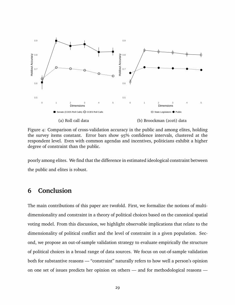
These two comparisons are shown in Figure 4. The pattern is the same in both: the ideal

point models perform much better among elites than they do in the public. The left-hand

side of the plot shows the roll-call measures for the Senate and the CCES. Despite including

only 8 roll-call votes in the Senate, a unidimensional model accurately classifies nearly

90 percent of votes — compared to less than 60 percent in the intercept-only model. In

contrast, the accuracy among the public on the exact same questions goes from 63 percent

to 71 percent. The right-hand panel tells a similar story for when the survey context is held

fixed.

These results suggest that the driving force behind the divergent performance of ideal

point models in the public relative to elites is primarily the differing levels of constraint

— not a different agenda, nor different incentives faced by actors operating in public and

private. If surveys are in fact poor tools for measuring opinion, they should also perform

28

●

● ●●

●●

0.5

0.6

0.7

0.8

0.9

0 1 2 3 4 5Dimensions

Hol

dout

Acc

urac

y

●Senate (CCES Roll Calls) CCES Roll Calls

(a) Roll call data

●

● ● ● ● ●

0.5

0.6

0.7

0.8

0.9

0 1 2 3 4 5Dimensions

Hol

dout

Acc

urac

y

●State Legislators Public

(b) Broockman (2016) data

Figure 4: Comparison of cross-validation accuracy in the public and among elites, holdingthe survey items constant. Error bars show 95% confidence intervals, clustered at therespondent level. Even with common agendas and incentives, politicians exhibit a higherdegree of constraint than the public.

poorly among elites. We find that the difference in estimated ideological constraint between

the public and elites is robust.

6 Conclusion

The main contributions of this paper are twofold. First, we formalize the notions of multi-

dimensionality and constraint in a theory of political choices based on the canonical spatial

voting model. From this discussion, we highlight observable implications that relate to the

dimensionality of political conflict and the level of constraint in a given population. Sec-

ond, we propose an out-of-sample validation strategy to evaluate empirically the structure

of political choices in a broad range of data sources. We focus on out-of-sample validation

both for substantive reasons — “constraint” naturally refers to how well a person’s opinion

on one set of issues predicts her opinion on others — and for methodological reasons —

29

in-sample measures of model fit are biased towards finding more dimensions and more

constraint than are actually present.

The importance of out-of-sample validation is apparent from our empirical results: we

find that ideal point models that contain more than a single dimension tend to search for

patterns in noise that makes it appear that there is more structure in the data than there

actually is. Political choices in the the United States, whether by survey respondents or

Senators, are best approximated as unidimensional.

In the Senate, this result is unsurprising. However, conventional wisdom holds that

political opinions among the mass public may be more nuanced than a single left-right

scale, implying that a higher-dimensional structure may exist. We find no evidence of such

a higher-dimensional structure. If anything, moving beyond a single dimension tends to

produce worse inferences in the public than among politicians.

Next, we turn to the issue of constraint. We operationalize constraint as the increase

in predictive performance that can be achieved by a model that explicitly incorporates an

actor’s ideal point, relative to an appropriately chosen null model. Using cross-validation,

we show that political elites are highly constrained, while members of the mass public

are relatively unconstrained. About 2/3 of the choices among politicians that cannot be

predicted by an intercept-only model can be predicted when we estimate a model with a

unidimensional ideal point. In contrast, only about 20% of survey responses in the mass

public that are unpredictable in an intercept-only model become predictable when the

model includes an ideal point.

Using a series of paired data sets, we show that this difference in predictive performance

cannot be attributed to the survey instrument, nor to differences in the agenda, nor to

differing incentives faced by politicians and regular citizens. The most likely explanation,

in our view, is the most simple: politicians organize politics in a more systematic way than

most citizens. This conclusion is further bolstered by the fact that at least one subset of the

public — people who identify as liberal or conservative— show evidence of more constraint

30

than other members of the public. Certainly other, more politically-engaged subgroups of

the public (e.g., donors) would also demonstrate higher levels of constraint.

Substantively, these results suggest caution when applying ideal point models to survey

responses from the mass public. While the public is best approximated as having unidimen-

sional ideal points, this ideal point does not predict attitudes on any given issue particularly

well. In the public, it appears that idiosyncratic, rather than ideological, preferences explain

the majority of voter attitudes. Our work suggests that scholars of public opinion should

pay heed to both ideological and idiosyncratic portions of policy attitudes.

31

References

Achen, Christopher H. 1975. “Mass Political Attitudes and the Survey Response.” American

Political Science Review 69(4):1218–1231.

Ansolabehere, Stephen, Jonathan Rodden and James M Snyder. 2006. “Purple America.”

Journal of Economic Perspectives 20(2):97–118.

Ansolabehere, Stephen, Jonathan Rodden and James M. Snyder. 2008. “The Strength of

Issues: Using Multiple Measures to Gauge Preference Stability, Ideological Constraint,

and Issue Voting.” American Political Science Review 102(02):215–232.

Bafumi, Joseph and Michael C. Herron. 2010. “Leapfrog Representation and Extremism: A

Study of American Voters and Their Members in Congress.” American Political Science

Review 104(03):519–542.

Barber, Michael and Jeremy C Pope. 2016. “Lost in Issue Space? Measuring Levels of

Ideology in the American Public.”.

URL: https://apw.polisci.wisc.edu/APW_Papers/scalingvoters_1.pdf

Barberá, Pablo. 2015. “Birds of the Same Feather Tweet Together: Bayesian Ideal Point

Estimation Using Twitter Data.” Political Analysis 23:76–91.

Berinsky, Adam J. 2017. “Telling the Truth about Believing the Lies? Evidence for the

Limited Prevalence of Expressive Survey Responding.” Journal of Politics 80(1):211–224.

Bond, Robert and Solomon Messing. 2015. “Quantifying Social Media’s Political Space:

Estimating Ideology from Publicly Revealed Preferences on Facebook.” American Political

Science Review 109(1):62–78.

Bonica, Adam. 2013. “Ideology and Interests in the Political Marketplace.” American

Journal of Political Science 57(2):294–311.

Broockman, David E. 2016. “Approaches to Studying Policy Representation.” Legislative

Studies Quarterly 41(1):181–215.

Bullock, John G., Alan S. Gerber, Seth J. Hill and Gregory A. Huber. 2015. “Partisan Bias in

Factual Beliefs about Politics.” Quarterly Journal of Political Science 10(4):519–578.

32

Campbell, Angus, Phillip Converse, Warren Miller and Donald Stokes. 1960. The American

Voter. Chicago: Chicago University Press.

Clinton, Joshua D, Simon Jackman and Douglas Rivers. 2004. “The Statistical Analysis of

Roll Call Data.” American Political Science Review 98(2):355–370.

Converse, Philip E. 1964. The Nature of Belief Systems in Mass Publics. In Ideology and

Discontent, ed. David Apter. New York: The Free Press pp. 206–261.

Downs, Anthony. 1957. An Economic Theory of Democracy. New York: Columbia University

Press.

Freeder, Sean, Gabriel S Lenz and Shad Turney. Forthcoming. “The Importance of

Knowing ‘What Goes With What’: Reinterpreting the Evidence on Policy Attitude

Stability.” Journal of Politics .

Hastie, Trevor, Robert Tibshirani and Jerome Friedman. 2009. Elements of Statistical

Learning: Data Mining, Inference, and Prediction. 2 ed. New York: Springer.

Heckman, James J. and James M. Snyder. 1997. “Linear Probability Models of the Demand

for Attributes with an Empirical Application to Estimating the Preferences of

Legislators.” The RAND Journal of Economics 28(0):S142–S189.

Hill, Seth J and Chris Tausanovitch. 2015. “A Disconnect in Representation? Comparison

of Trends in Congressional and Public Polarization.” Journal of Politics 77(4):1058–1075.

Imai, Kosuke, James Lo and Jonathan Olmsted. 2016. “Fast Estimation of Ideal Points with

Massive Data.” American Political Science Review 110(4):1–20.

Jackman, Simon. 2001. “Multidimensional Analysis of Roll Call Data via Bayesian

Simulation: Identification, Estimation, Inference, and Model Checking.” Political

Analysis 9(3):227–241.

Jessee, Stephen A. 2009. “Spatial Voting in the 2004 Presidential Election.” American

Political Science Review 103(01):59.

Kinder, Donald R. 2003. Belief Systems After Converse. In Electoral Democracy, ed.

Michael MacKuen and George Rabinowitz. Ann Arbor: University of Michigan Press.

33

Kuklinski, James H. and Paul J. Quirk. 2000. Reconsidering the Rational Public:

Cognition, Heuristics, and Mass Opinion. In Elements of Reason: Cognition, Choice, and

the Bounds of Rationality, ed. Arthur Lupia, Matthew D. McCubbins and Samuel L.

Popkin. Cambridge University Press.

Lauderdale, Benjamin E., Chris Hanretty and Nick Vivyan. 2017. “Decomposing Public

Opinion Variation into Ideology, Idiosyncrasy and Instability.” Journal of Politics pp. 1–9.

Little, Roderick J A and Donald B Rubin. 1983. “On Jointly Estimating Parameters and

Missing Data by Maximizing the Complete-Data Likelihood.” Journal of the American

Statistical Assocation 37(3):218–220.

Little, Roderick J A and Donald B Rubin. 2014. Statistical Analysis with Missing Data. 2nd

ed. Hoboken, NJ: John Wiley & Sons.

Marcus, George E, David Tabb and John L Sullivan. 1974. “The Application of Individual

Differences Scaling to the Measurement of Political Ideologies.” American Journal of

Political Science 18(2):405–420.

Mnih, Andriy and Ruslan R Salakhutdinov. 2008. Probabilistic matrix factorization. In

Advances in neural information processing systems. pp. 1257–1264.

Pan, Jennifer and Yiqing Xu. 2018. “China’s Ideological Spectrum.” Journal of Politics

80(1):254–273.

Poole, Keith T. and Howard Rosenthal. 1997. Congress: A Political-Economic History of Roll

Call Voting. Oxford University Press.

Rivers, Douglas. 2003. “Identification of Multidimensional Spatial Voting Models.”.

Salakhutdinov, Ruslan and Andriy Mnih. 2008. Bayesian probabilistic matrix factorization

using Markov chain Monte Carlo. In Proceedings of the 25th international conference on

Machine learning. ACM pp. 880–887.

Schaffner, Brian F and Samantha Luks. 2018. “Misinformation or Expressive Responding?

What an Inauguration Crowd Can Tell Us About the Source of Political Misinformation

in Surveys.” Public Opinion Quarterly .

34

Shor, Boris and Nolan M. McCarty. 2011. “The Ideological Mapping of American

Legislatures.” American Political Science Review 105(3):530–551.

Tausanovitch, Chris and Christopher Warshaw. 2013. “Measuring Constituent Policy

Preferences in Congress, State Legislatures, and Cities.” Journal of Politics

75(02):330–342.

Tausanovitch, Chris and Christopher Warshaw. 2017. “Estimating Candidate Positions in a

Polarized Congress.” Political Analysis .

Treier, S. and D. S. Hillygus. 2009. “The Nature of Political Ideology in the Contemporary

Electorate.” Public Opinion Quarterly 73(4):679–703.

35

Supplementary Materials

Table of ContentsA Technical Appendix: MultiScale Algorithm 2

B External Validation for the MultiScale Algorithm 4

C Simulation Study of Cross-Validation Estimator 6

D Data Appendix 8

E Alternative Measure of Fit 12

1

A Technical Appendix: MultiScale Algorithm

The Parametric Model

N voters and J binary questions to vote on. The vote matrix is Y ∈ {0, 1}N× J . For someD ∈ N, Let αj ∈ R, βj ∈ R

D and γi ∈ RD for each j = 1, . . . , J and i = 1, . . . , N . We assume

the following latent variable model generates the binary vote matrix Y .

yi j = I (si j > 0)

si j = αj + β′jγi + εi j, εi j

ind.∼ N (0, 1),

wherewe have assumedσ = 1, since it is not identified. Note that for θ = ({αj }Jj=1, {βj }

Jj=1, {γi }

Ni=1),

this implies the reduced form likelihood

p(Y | θ) =N∏

i=1

J∏j=1

[Φ(αj + β

′jγi )

]yi j[1 − Φ(αj + β

′jγi )

]1−yi j

.

Let R ∈ {0, 1}N× J denote the matrix of observation statuses. That is ri j = 1, if the (i, j )thcell ofY is observed and ri j = 0 if it is missing. We assume the data are missing at random,P (R | Yobs, Ymis, θ, ω) = P (R | Yobs, θ, ω), and that the parameters ω that determine R aredistinct from the structural voting parameters θ, meaning that we can ignore the likelihoodof R (section 6.2, Little and Rubin, 2014). The resulting (ignorable) likelihood is

p(Yobs | θ) =

N∏i=1

J∏j=1

{[Φ(αj + β

′jγi )

]yi j[1 − Φ(αj + β

′jγi )

]1−yi j}ri j

.

We assume standard priors on θ; specifically,

ξ(θ) =

J∏j=1

N

( [αj

βj

]; µab, Σab

) N∏i=1

N(γi ; µγ, Σγ

),

where µab ∈ RD+1, µγ ∈ Rd and Σab ∈ R

(D+1)×(D+1), Σγ ∈ RD×D are positive definite matrices.

The Algorithm

We consider just the log likelihood to illustrate how we extend the algorithm of Imai, Loand Olmsted (2016). Let mi j = αj + β

′jγi and Sobs be the values of S that correspond to the

Y observed values Yobs. The complete-data (complete here is with respect to Sobs, not the

2

values of Y for which ri j = 0) log likelihood is given by

log p(Yobs, Sobs | θ)

= logN∏

i=1

J∏j=1

[N (si j | mi j, 1)

]ri j

(I (yi j=1)I (si j≥0)+I (yi j=0)I (si j<0)

)

=

N∑i=1

J∑j=1

ri j

(I (yi j = 1)I (si j ≥ 0) + I (yi j = 0)I (si j < 0)

)logN (si j ;mi j, 1).

But this is the same complete-data log likelihood found in Imai, Lo and Olmsted (2016,Appendix A), except for the insistence on only using the observed data as observations.Therefore we can take their update equations and restrict ourselves to only using observeddata. Specifically, iterate between

si j ← mi j + (2yi j − 1)φ(mi j )

Φ((2yi j − 1)mi j

)γi ←

©­«Σ−1γ +J∑

j=1

ri j βj β′jª®¬−1 ©­«Σ−1γ µγ +

J∑j=1

ri j βj (si j − αj )ª®¬

[αj

βj

]←

(Σ−1ab +

N∑i=1

ri j

[1γi

] [1γi

]′)−1 (Σ−1ab µab +

N∑i=1

ri j si j

[1γi

]).

3

B External Validation for the MultiScale Algorithm

In the following figures, we plot several validation measure for the MultiScale algorithm.They show that for several data sources, the MultiScale estimates correlate highly withother measures of ideology.

0

1

2

−1.0 −0.5 0.0 0.5 1.0

1D MultiScale 109th Senate Score

Den

sity

Democrats Republicans

MultiScale Score by Party, 109th Senate

(a)

●

●

●

●

●

●

●

●

●

●

●

●

● ●●

●

●

●

●

●

●

●

●

●

●●

●●

●

●

●

●

●

●

●

●

●

●

●

●

●

●

●

●

●

●

● ●

●

●

●

●

●

●

●

●

●

●●

●

●

●

● ●

●

●

●

●

●

●

●

●

●

●●

●

●

●

●

●

●

●

●●

●

●

●

●

●

●

●

●

●

●

●●

r = 0.97

−1.0

−0.5

0.0

0.5

1.0

−0.50 −0.25 0.00 0.25 0.50

DWNOMINATE

1D M

ultiS

cale

109

th S

enat

e S

core

MultiScale Score vs. DWNOMINATE, 109th Senate

(b)

Figure 1: Comparison of MultiScale ideal points among Senators in the 109th Congress.The left-hand side shows that Democrats are almost universally to the left of Republi-cans. The right-hand side shows that MultiScale scores are highly correlated with DW-NOMINATE scores.

0.00

0.25

0.50

0.75

1.00

−1 0 1

1D MultiScale NPAT Score

Den

sity

Democrats Republicans

MultiScale Score by Party, NPAT Data

(a)

●

●

●

●

●

●

●

●

●

●

●

●

●

●

●

●

●

●

●

●

●

●

●

●

●

●

●

●

●

●

●

●

●

●

●

●

●

●

●

●

●

●

●

●

●

●

●

●

●

●

●

●

●

●

●

●

●

●

●

●

●

●

●

●

●

●

●

●

●

●

●

●

●

●

●

●

●

●

●

●

●

●

●

●

●

●

●

●

●

●

●

●

●

●

●

●

●

●

●

●

●

●

●

●

●

●

●●

●

●

●

●

●

●

●

●

●

●

●

●

●

●

●

●

●

●

●

●

●

●

●

●

●

●

●

●

●

●

●

●

●

●

●

●

●

●

●

●

●

●

●

●

●

●

●

●

●

●

●

●

●

●

●

●

●

●

●

●

●

●

●

●

●

●

●

●

●

●

●

●

●

●

●

●

●

●

●

●

●

●

●

●

●

●

●

●

●

●

●

●

●

●●

●

●

●

●

●

●

●

●

●

●

●

●

●

●

●

●

●

●

●

●

●

●

●

●

●

●

●

●

●

●

●

●

●

●●

● ●●

●

●

●

●●

●

●

●

●

●

●

●

●

●

●

●

●

●

●

●

●

●

●

●

●

●

●

●

●

●

●

●

●

●●

●●

●

●

●

●

●

●

●

●

●

●

●

●

●

●

●

●●

●

●

●

●

●

●

●

●

●

●

●

●

●

●●

● ●

●

●

●

●

●

●

●

●

●

●

●

●

●

●

●

●

●

●

●

●

●

●

●

●

●

●

●

●

●

●

●

●

●

●

●

●

●

●●

●

●

●

●

●

●

●

●

●

●

●

●●

●

●

●

●

●

●

●

●

●

●

●

●

●

●

●

●

●

●

●●

●

●

●

●

●

●

●

●

●

●

●

●

●

●

●

●

●

●

●

●

●

●

●

●

●

●

●

●

●

●

●

●

●

●

●

●

●

●

●

●

●

●

●

●

●

●

● ●

●

●

●

●

●

●

●

●

●

●

●

●

●

●

●

●

●

●

●

●

●

●

●

●

●

●

●

●

●

●

●

●

●

●

●

●

●

●

●

●

●

●

●

●

●

●

●

●

●

●

●

●

●

●

●

●

●

●

●

●

●

●

●

●

●

●

●

●

●

●

●

●●

●

●

●

●

●

●

●

●

●

●●

●

●

●

●

●

●

●

●

●

●

●

●

●

●

●

●

●

●

●

●

●

●

●

●

●

●

●

●

●

●

●

●

●

●

●

●●

●

●

●

●

●

●

●

●

●

●

●

●

●

●

●

●

●

●

●

●

●

●

●

●

●

●

●

●

●

●

●

●

●

●

●

●

●

●●

●

●

●

●

●

●

●

●

●

●

●

●

●

●

●

●

●

●

●

●

●

●

●

●

●

●

●

●

●

●

●

●

●

●

●

●

●

●

●

●

●

●

●

●

● ●

●

●

●

●

●

●

●

●

●

●

●

●

●

●

●

●

●

●

●

●

●

●

●

●

●

●

●

●

●

●

●

●

●

●

●

●

●

●

●

●

●

●

●

●

●

●●

●

●

●

●

●

●

●

●

●

●

●

●

●

●●

●

●

●

●

●

●

●

●

●

●

●

●

●

●

●

●

●

●

●

●

●

●

●

●

●

●

●

●

●

●

●

●

●

●

●

●

●

●

●

●

●

●

●

●

●

●

●

●

●

●

●

●

●

●

●

●

●

●

●

●

●

●

●

●

●

●

●

●

●

●

●

●

●

●

●

●

●

●

●

●

●

●

●

●

●

●

●●

●

●

●

●

●

●

●

●

●

●

●

●

●

●

●

●

●

●

●

●

●

●

●

●

●

●

●

●

●

●

●

●

●

●

●

●

●

●

●

●

●

●

●

●

●

●

●

●

●

●

●

●

●

●

●

●

●

●

●

●

●

●

●

●

●

●

●

●

●

●

●

●

●

●

●

●●

●

●

●

●

●

●

●

●

●

●

●

●

●

●

●

●

●●

●

●

●

●

●

●

●

●

●

●

●

●

●

●

●

●

●

●

●

●

●

●

●

●

●

●

●

●

●

●

●

●

●

●

●

●

●

●

●

●

●

●

●

●

●

●

●

●

●

●

●

●

●

●

●

●

●

●

●

●

●

●

●

●

●

●

●

●

●

●

●

●

●

●

●

●

●

●

●

●

●

●

●

●

●

●

●

●

●

●

●

●

●

●

●

●

●

●

●

●

●

●

●

●

●

●

●

●

●

●

●

●

●

●

●

●

●

●

●

●

●

●

●

●

●

●

●

●

●

●

●

●

●

●

●

●

●

●

●

●

●

●

●

●

●

●

●

●

●●

●

●

●

●

●

●

●

●

●

●

●

●

●

●

●

●

●

●

● ●

●

●

●

●

●

●

●

●

●●

●

●

●

●

●

●

●

●

●

●●

●●

●

●

●

●

●

●

●

●

●

●

●

●

●

●

●

●

●

●

●

●

●

●

●

●

●

●

●

●

●

●

●

●

●

●

●

●

●

●

●

●

●

●

●

●

●

●

●

●

●

●

●

●

●

●

●

●

●

●

●

●

●

●

●

●

●

●

●

●

●

●

●

●

●

●

●

●

●

●

●

●

●●

●

●

●

●

●

●

●

●

●

●

●

●

●

●

●

●

●

●

●

●

●

●

●

●

●

● ●

●

●

●

●

●

●●

●

●

●

●

●●

●

●

●

●

●

●

●

●

●

●

●

●

●

●

●

●

●

●●

●

●●

●

●

●

●

●

●

●

●

●

●

●

●

●

●

●

●

● ●

●

●

●

●●

●

●

●●

●

●

●

●

●

●

●

●

●

●

●

●

●

●

●

●

●

●

●

●

●

●

●

●

●

●

●

●

●

●

●

●

●

●

●

●

●

●

●

●

●

●

●

●

●

●

●

●

●

●

●

●

●

●

●

●

●

●

●

●

●

●

●

●

●

●

●

●

●

●

●

●

●

●

●

●

●

●

●

●

●

●

●

●

●

●

●

●

●

●

●

●

●

●

●

● ●

●

●

●

●

●

●

●

●

●

●

●

●

●

●

●

●

●

●

●

●

●

●

●

●

●

●

●

●

●

●

●

●

●

●

●

●

●

●

●

●

●

●

●

●

●

●

●

●

●

●

●

●

●

●

●

●

●

●

●

●

●

●

●

●

●

●

●

●

●

●

●

●

●

●

●

●

●

●

●

●

●

●

●

●

●

●

●

●

●

●

●

●

●

●

●

●

●

●

●

●

●

●

●

●

●

●

●

●

●

●

●

●

●

●

●

●

●

●

●

●

●

●

●

●

●

●

●

●

●

●

●

●

●

●

●

●

●●

●

●

●

●

●

●

●

●●

●

●

●

●

●

●

●

●

●

●

●

●

●

●

●

●

●

●

●

●

●

●

●

●

●

●

●

●

●

●

●

●

●

● ●

●

●

●

●

●

●

●

●

●

●

●

●

●

●

●

●

●

●

●

●

●

●

●

●

●

●

●

●

●

●

●

●

●

●

●●

●

●

●

●

●

●

●

●

●

●

●

●

●

●

●

●

●

●

●

●

●

●

●

●

●

●

●

●

●

●

●

●

●

●

●

●

●

●

●

●

●

●

●

●

●

●

●

●

●

●

●

●

●

●

●

●

●

●

●

●

●

●

●

●●

●

●

●

●

●

●

●

●

●

●

●

●

●

●

●

●

●

●

●

●

●

●

●

●

●

●

●

●

●

●

●

●●

●

●

●

●

●

●

●

●

●

●

●

●

●

●

●

●

●

●

●

●

●

●

●

●

●

●

●

●

●

●

●

●

●

●

●

●

●

●

●

●●

●

●

●

●

●

●

●

●

●

●

●

●

●

●

● ●

●

●

●

●

●

●

●

●

●

●

●

●

●

●

●

●

●

●

●

●

●

●

●

●

●

●

●

●●

●

●

●

●

●

●

●

●●

●

●

●

●

●

●

●

●

●

●

●●

●

●

●

●

●

●

●

●

●

●

●

●

●

●

●

●

●

●

●

●

●

●

●

●

●

●

●

●

●

●

●

●

●

●

●

●

●

●

●

●

●

●

●

●

●

●

●

●

●

●

●

●

●

●

●

●

●

●

●

●

●

●

●

●

●

●

●

●

●

●

●

●

●

●

●

●

●

●

●

●

●

●

●

●

●

●

●

●

●

●

●● ●

●

●

●

●

●

●

●

●

●

●

●

●

●

●

●

●

●●

●

●

●

●

●

●

●

●

●

●

●

●

●

●

●

●

●

●

●

●

●

●

●

●

●

●

●

●

●

●

●

●

●

●

●

●

●

●

●

●

●

●

●

●

●

●

●

●

●

●

●

●

●

●

●

●

●

●

●

●

●

●

●

●

●

●

●

●

●

●

●

●

●

●

●

●

●

●

●

●

●

●

●

●

●

●

●

●

●●

●●

●

●

●

●

●

●

●

●

●

●

●

●

●

●

●

●

●

●

● ●

●

●

●

●

●

●

●

●

●

●

●

●

●

●

●

●

●

●

●

●

●

●

●

●

●

●

●

●

●

●

●

●

●

●

●

●●

●

●

●

●

●

●

●

●

●●

●

●

●

●

●●

●

●

●

●

●●

●

●

●

●

●

●

●

●

●

●

●

●

●

●

●

●

●

●

●

●

●

●

●

●

●

●

●

●

●

●

●

●

●

●

●

●

●

●●

●

●

●

●

●●

●

●

●

●

●

●

●

●

●

●

●

●

●●

●

●

●

●

●

●

●

●

●

●

●

●

●

●

●

●

●

●

●

●

●

●

●

●

●

●

●

● ●

●

●

●

●

●

●

●

●

●

●

●

● ●

●

●

●

●

●

●

●

●

●

●

●

●

●

●

●

●

●

●

●

●

●

●

●

●

●

●

●

●●

●

●

●

●

●

●

●

●

●

●

●

●

●

●

●

●

●

●

●

●

●●

●

●

●

●

●

●

●●

●

●

●

●

●●

●

●

●

●

●

●

●

●

●

●

●

●

●

●

●

●

●

●

●

●

●

●

●

●

●

●

●

●

●

●

●

●

●

●

●

●

●

●

●

●

●

●

●

●

●

●

●

●

●

●

●

●

●

●

●

●

●

●

●

●

●

●

●

●

●

●

●

●

●

●

●

●

●

●

●

●

●

●

●

●

●

●

●

●

●

●

●

●

●

●

●

●

●

●

●

●

●

●

●

●

●

●

●

●

●

●

●

●

●

●

●

●

●

●

●

●

●

●

●

●

●

●

●

●

●

●

●

●

●

●

●

●

●● ●

●

●

●

●

●

●

●

●

●

●

●

●

●

●

●

●

●

●

●

●

●

●

●

●

●

●

●

●

●

●

●

●

●

●

●

●

●

●

●

●

●

●

●

●

● ●

●

●

●

●

●

●

●

●

●

●

●

●

●

●

●

●

●

●

●

●

●

●

●

●

●

●

●

●

●

●

●

●

●

●

●

●

●●

●

●

●

●

●

●

●

●

●

●

●

●

●

●

●

●

●

●

●

●

●

●

●

●

●

●

●

●

●

●

●

●

●

●

●

●

●

●

●

●

●

●

●

●

●

●

●

●

●

●

●

●

●

●

●

●

●

●

●

●

●

●

●

●

●

●

●

●

●

●

●

●

●

●●

●

●

●

● ●

●

●

●

●●

●

●

●

●

●

●

●

●

●

●

●

●

●

●

●

●

●

●

●

●

●

●

●

●

●

●

●

●

●

●●

●

●

●

●

●

●●

●

●

●

●

●

●

●

●

●

●

●

●

●

●

●

●

●

●

●

●

●

●

●

●

●

●

●

●

●

●

●

●

●

●

●

●

●

●

●

●

●

●

●

●

●

●

●

●

●

●

●

●

●

●

●

●

●

●

●

●

●

●

●

●

●

●

●

●

●

●●

●

●●

●

●

●

●

●

●

●

●

●

●

●

●

●

●

●

●

●

●

●

●

●

●

●

●

●

●

●

●

●

●

●

●

●

●

●

●

●

●

●

●

●

●

●

●

●

●

●

●

●

●

●

●

●

●

●

●

●

●

●

●

●

●

●

●

●

●

●

●

●●

●

●

●

●

●

●

●

●

●

●

●●

●

●

●

●

●

●

●

●

●

●

●

●

●●

●

●

●

●

●

●

●

●

●

●

●

●

●

●

●

●

●

●

●

●

●

●

●

●

●

●

●

●

●

●

●

●

●

●

●

●

●

●

●

●

●

●

●

●

●

●

●

●

●

●

●

●

●

●

●

●

●

●

●

● ●

●

●

●

●

●

●

●

●

●

●

●

●

●

●

●

●

●

●

●

●

●

●

●

●

●

●

●

●

●

●

●

●

●

●

●

●

●

●

●

●

●

●

●

●

●

●

●

●

●

●

●

●

●

●

●

●

●

●●

●

●

●

●

●

●

●

●

●

●

●

●

●

●

●

●

●

●

●

●

●

●

●

●

●

●

●

●

●

●

●●

●

●

●

●

●

●

●

●

●

●

●

●

●

●

●

●

●

●

●

●

●●

●

●

●

●

●

●

●

●

●

●

●

●

●

●●

●

●

●●

●

●

●

●

●

●

●

●

●

●

●

●

●

●

●

●

●

●

●

●

●

●

●

●

●

●

●

●

●●

●

●

●

●

●

●

●

●

●

●

●

●

●

●

●

●

●

●

●

●

●

●

●

●

●

●

●

●

●

●

●

●

●

●

●

●

●

●

●

●

●

●

●

●

●

●●

●●

●

●

●

●

● ●

●

●

●●

●

●

●

●

●

●

●

●

●

●

●

●

●

●

●

●

●

●

●

●

●

●●

●

●

●

●

●

●

●

●

●

●

●

●

●

●

●

●

●

●

●

●

●

●

●

●

●●

●

●

●

●

●

●

●

●

●

●

●

●

●

●

●

●

●

●

●

●

●

●

●

●

●

●

●

●

●

●

●

●

●

●

●

●

●●

●

●

●

●

●

●

●

●

●

●

●

●

●

●

●

●

●

●

●

●

●

●

●

●

●●

●

●

●

●

●●

●

●

●

●

●

●

●

●

●

●

●

●

●

●

●

●

●

●

●

●

●

●

●

●

●

●

●

●

●

●

●

●

●

●

●●

●

●

●

●

●

●

●

●

●

●

●

●

●

●

●

●

●

●

●

●

●

●

●

●

●

●●

●

●

●

●

●

●

●

●

●

●

●

●

●

●

●

●

●

●

●

●

●

●

●

●

●●

●

●

●

●

●

●

●

●

●

●

●

●

●

● ●

●

●

●●

●

●

●

●

●

●

●

●

●

●

●

●●

●

●

●

●

●

●

●

●

●

●

●

●

●

●

●

●

●

●

●

●

●

●

●

●

●

●

●

●

●

●

●

●

●

●

●

●●

●

●

●

●

●

●

●

●

●

●

●

●

●

●

●

●

●

●

●

●●

●

●

●

●●

●

●

●

●

●

●

●●

●

●

●

●

●

●

●

●

●

●

●

●

●

●

●

●

●

●

●

●

●

●

●

●

●

●

●

●

●

●

●

●

●

●

●

●

●

●

●

●

●

●

●

●

●

●

●

●

●

●

●

●

●

●

●

●

●

●●

●

●

●

●

●

●

●

●

●

●

●

●

●

●

●

●

●

●

●

●

●

●

●

●

●

●

●

●

●

●

●

●

●

●

●

●

●

●

●●

●

● ●

●

●

● ● ●●

●

●

●

●

●

●

●

●

●

●

●

●

●

●

●

●

●

●

●

●

●

●

●

●●

●

●

●

●

●

●

●

●

●

●

●

●

●

●

●

●

●

●

●

●

●

●

●

●

●

●

●

●

●

●

●

●

●

●

● ●

●

●

●

●

●

●

●

●

●

●

●

●

●

●

●

●

●

●

●

●

●

●

●

●

●

●

●

●

●

●

●

●

●

●

●

●

●

●

●

●

●

●

●

●

●

●

●

●

●

●

●

●

●

●

●

●

●

●

●

●

●

●

●

●

●

●

●

●

●

●

●

●

●●

●

●

●

●

●

●

●

●

●

●

●

●

●

●

●

●●

●

●

●●

●

●

●

●

●●

●

●

●

●

●

●

●

●

●

●

●

●

●

●

●

●

●

●

●

●

●

●

●

●

●

●

●

●

●

●

● ●

●

●

●

●

●

●

●

●

●

●

●

●

●

●

●

●

●

●

●

●

●

●

●

●

●

●

●

●

●

●

●

●

●

●

●

●

●

●

●

●

●

●

●

●

●

●

●

●

●

●

●

●

●

●

●●

●

●

●

●

●

●

●

●

●

●

●

●●

●

●

●

●

●

●

●

●

●

●

●

●

●

●

●

●●

●

●

●●

●

●

●

●

●

●

●

●

●

●

●

●

●

●

●

●

●

●

●

●

●

●

●

●

●

●

●

●

●

●

●

●

●

●

●

●

●

●

●

●

●

●

●

●

●

●

●

●

●

●

●

●

●

●

●

●

●

●

●

●

●

●

●

●

●

●

●

●

●

●

●

●

●

●

●

●

●

●

●

●

●

●

●

●●

●

●

●

●

●

●

●

●

●

●

●

●

● ●

●

●

●

●

●

●

●

●

●

● ●

●

●

●

●

●●

●

●

●

●

●

●

●

●

●

●

●

●

●

●

●

●

●

●

●

●

●

●

●

●

●

●

●

●

●●

●

●

●

●

●

●

●

●●

●

●

●

●

●

●

●

●

●

●

●

●

●

●

●●

●

●

●

●

●

●

●

●

●

●

●

●

●

●

●

●

●

●

●

●

●

●

●

●

●

●

●

●

●●

●

●

●

●

●

●

●

●

●

●

●

●

●

●

●●

●

●

●

●

●

●

●

●

●

●

●

●

●

●

●

●

●

●

●

●

●

●

●

●

●

●

●●

●

●

●

●

●

●

●

●

●●

●

●

●

●

●

●

●

●

●

●

●

●

●

●

●

●

●

●

●

●

●

●

●

●

●

●

●

●

●

●

●

●

●

●

●

●

●

●

●

●

●

●

●

●

●

●

●

●

●

●

●

●

●

●

●

●

●

●

●

●

●

●

●

●

●

●

●

●

●●

●

●

●

●

●

●

●

●

●

●

●

●

●

●

●

●

●

●

●

●

●

●

●

●

●

●

●

●

●

●

●

●

●

●

●●

●

●

●

●●

●

●

●

●

●

●

●

●

●

●

●

●

●

●

●

●

●

●

●

●

●

●

●

●

●

●

●

●

●

●

●

●

●

●

●

●

●

● ●

●

●

●

●

●

●

●

●

●

●

●

●

●

●

●

●

●

●

●

●

●

●

●

●

●

●

●

●

●

●

●

●

●

●

●

●

●

●●

●

●

●

●

●

●

●

●

●

●

●

●

●

●

●

●

●

●

●

●

●

●

●

●

●

●

●

●

●

●

●

●

●

●

●

●

●

●

●

●

●●

●

●

●

●

●

●

●

●

●

●

●

●

●

●

●

●

●

●

●

●

●

●

●

●

●

●

● ●

●

●

●

●

●

●

●

●

●

●

●

●

●

●

●

●

●

●

●

●

●

●

●

●

●

●

●

●

●

●

●

●

●

●●

●

●

●

●

●

●

●

●

●

●

●

●

●

●

●

●

●

●

●

●

●

●

●

●

●

●

●

●

●

●

●

●

●

●

●

●

●

●

●

●

●

●

●

●

●

●

●

●

●

●

●

●

●

●

●

●

●

●

●

●

●

●

●

r = 0.86

−1

0

1

−2 0 2

Shor−McCarty NPAT Score

1D M

ultiS

cale

NPA

T S

core

MultiScale Score vs. Shor−McCarty NPAT Score, Full Data

(b)

Figure 2: Comparison of MultiScale ideal points among politicians using NPAT data. Theleft-hand side shows that Democrats are consistently to the left of Republicans. The right-hand panel shows the correlation between MultiScale scores estimated with the NPAT datato the Shor-McCarty NPAT scores.

4

0.0

0.4

0.8

1.2

−1 0 1

1D MultiScale ANES 2012 Scores

Den

sity

Democrat Independent Republican

MultiScale Score by Party, ANES 2012

Figure 3: Comparison of MultiScale ideal points from the ANES by party.

5

● ● ● ● ● ●

●

●

● ● ● ●

●

●

●

●

● ●

●

● ● ● ● ●

●

●

●

● ● ●

●

●

●

●

●

●

True Dimensions: 4 True Dimensions: 5

True Dimensions: 2 True Dimensions: 3

True Dimensions: 0 True Dimensions: 1

0 1 2 3 4 5 0 1 2 3 4 5

0.6

0.7

0.8

0.9

0.6

0.7

0.8

0.9

0.6

0.7

0.8

0.9

Assumed Dimensionality

Acc

urac

yN = 102, J = 645

● ●● ● ●

●

●

●

●●

●●

●

●

●

●

●●

●

● ●●

●●

●

●

●

●●

●

●

●

●

●

●●

True Dimensions: 4 True Dimensions: 5

True Dimensions: 2 True Dimensions: 3

True Dimensions: 0 True Dimensions: 1

0 1 2 3 4 5 0 1 2 3 4 5

0.5

0.6

0.7

0.8

0.9

0.5

0.6

0.7

0.8

0.9

0.5

0.6

0.7

0.8

0.9

Assumed Dimensionality

Acc

urac

y

N = 1000, J = 20

Figure 4: Simulation results. Left-hand panel shows Senate-sized data; right-hand panelshows ANES-sized data. Dotted vertical lines indicate the dimensionality of the true data-generating process.

C Simulation Study of Cross-Validation Estimator

To illustrate that our proposed method of out-of-sample validation can accurately recoverthe latent dimensionality of political choices, we conduct a small simulation study.

We simulate data sets according to the spatial voting model laid out in Section 1 inthe main text. First, we fix the number of actors and choices (N and J , in the notationof the paper). Then, we simulate a series of choice matrices Y D generated according to aD ∈ {0, . . . , 5} dimensional ideal point model. In particular, the voter surplus for voter i onchoice j is modeled as

si j = αj + βDj′γD

i + εi j (7)

εi jind.∼ N (0, 1) (8)

Y Di j = I (si j > 0), (9)

where we explicitly denote the dimensionality with superscripts. We draw αj independentstandard normal (separately for each dimension) and γD

i from a multivariate standardnormal. To ensure that all D dimensions are in fact relevant to the choice, we restrict eachelement of βD

j to be either −1 or 1, chosen randomly.For each simulated data set, we run the cross-validation procedure outlined in the text.

We estimate the predictive error associated with estimating models that assume 0 to 5dimensions. If the cross-validation procedure can correctly measure the dimensionality ofthe data, the accuracy should be maximized when we estimate a model that assumes thesame dimensionality that the data were generated with.

6

We repeat this exercise twice. First, we simulate data sets that are approximately thesame size as the Senate data used in the main text, with N = 102 and J = 645. Second, wesimulate data sets approximately the same size as the ANES, with N = 1, 000 and J = 20.

The results are shown in Figure 4. The left-hand panel shows the results for the Senate-sized data and the right-hand panel shows the results for the ANES-sized data. In all cases,the estimated dimensionality is the same as the true dimensionality, providing evidencethat the validation strategy proposed in the paper can accurately recover the dimensionalityof the data-generating process.

7

D Data Appendix

Broockman (2016) State Legislator Variables

Variable Description

iq_vouchers The government should provide parents with vouchersto send their children to any school they choose, be itprivate, public, or religious. (Binary)

iq_medicalpot Allow doctors to prescribe marijuana to patients. (Bi-nary)

iq_taxesover250k Increase taxes for those making over $250,000 per year.(Binary)

iq_overturnroe Overturn Roe v. Wade. (Binary)iq_privitsocialsec Allow workers to invest a portion of their payroll tax

in private accounts that they can manage themselves.(Binary)

iq_gaymarriage Same-sex couples should be allowed to marry. (Binary)iq_unihealth Implement auniversal health care program to guarantee

coverage to all Americans, regardless of income. (Bi-nary)

iq_medlawsuits Limit the amount of punitive damages that can beawarded in medical malpractice lawsuits. (Binary)

iq_guncontrol There should be strong restrictions on the purchase andpossession of guns. (Binary)

iq_illegalim Illegal immigrants should not be allowed to enroll ingovernment food stamp programs. (Binary)

iq_enda Include sexual orientation in federal anti-discriminationlaws. (Binary)

iq_affaction Prohibit the use of affirmative action by state collegesand universities. (Binary)

iq_unfunding The US should contribute more funding and troops toUN peacekeeping missions. (Binary)

iq_fundarts The government should not provide any funding to thearts. (Binary)

iq_dealthpenalty I support the death penalty in my state. (Binary)iq_repealcapgainstax Repeal taxes on interest, dividends, and capital gains.

(Binary)iq_epaprohibit Prohibit the EPA from regulating greenhouse gas emis-

sions. (Binary)iq_birthcontrolmandate Health insurance plans should be required to fully cover

the cost of birth control. (Binary)iq_subsidizeloans The federal government should subsidize student loans

for low income students. (Binary)

8

eq_guns Which statement comes closest to describing your viewson gun control? (1-7 scale)

eq_health Which statement comes closest to describing your viewson the issue of health care? (1-7 scale)

eq_immigration Which statement comes closest to describing your viewson immigration? (1-7 scale)

eq_taxes Which statement comes closest to describing your viewson taxes? (1-7 scale)

eq_abortion Which statement comes closest to describing your viewson abortion? (1-7 scale)

eq_environment Which statement comes closest to describing your viewson pollution and the environment? (1-7 scale)

eq_medicare Which statement comes closest to describing your viewson Medicare, the government’s program for covering theelderly’s health care costs? (1-7 scale)

eq_gays Which statement comes closest to describing your viewson rights for gays and lesbians? (1-7 scale)

eq_affirmativeaction Which statement comes closest to describing your viewson affirmative action in higher education? (1-7 scale)

eq_unions Which statement comes closest to describing your viewson unions? (1-7 scale)

eq_education Which statement comes closest to describing your viewson public funding for private school education? (1-7scale)

eq_contraception_version2 Which statement comes closest to describing your viewson birth control? (1-7 scale)

9

2012 ANES Variables, from Hill and Tausanovitch (2015)

Variable Description

VCF0806 R Placement: Government Health Insurance ScaleVCF0809 R Placement: Guaranteed Jobs and Income ScaleVCF0823 R Opinion: Better off if U.S. Unconcerned with Rest of WorldVCF0830 R Placement: Aid to Blacks ScaleVCF0838 R Opinion: By Law, When Should Abortion Be AllowedVCF0839 R Placement: Government Services/Spending ScaleVCF0843 R Placement: Defense Spending ScaleVCF0867a R Opinion: Affirmative Action in Hiring/Promotion [2 of 2]VCF0876a R Opinion Strength: Law Against Homosexual DiscriminationVCF0877a R Opinion Strength: Favor/Oppose Gays in MilitaryVCF0878 R Opinion: Should Gays/Lesbians Be Able to Adopt ChildrenVCF0879a R Opinion: U.S. Immigrants Should Increase/Decrease [2 of 2]VCF0886 R Opinion: Federal Spending- Poor/Poor PeopleVCF0887 R Opinion: Federal Spending- Child CareVCF0888 R Opinion: Federal Spending- Dealing with CrimeVCF0889 R Opinion: Federal Spending- Aids Research/Fight AidsVCF0894 R Opinion: Federal Spending- Welfare ProgramsVCF9013 R Opinion: Society Ensure Equal Opportunity to SucceedVCF9014 R Opinion: We Have Gone Too Far Pushing Equal RightsVCF9015 R Opinion: Big Problem that Not Everyone Has Equal ChanceVCF9037 R Opinion: Government Ensure Fair Jobs for BlacksVCF9040 Blacks Should Not Have Special Favors to SucceedVCF9047 R Opinion: Federal Spending- Improve/Protect EnvironmentVCF9048 R Opinion: Federal Spending- Space/Science/TechnologyVCF9049 R Opinion: Federal Spending- Social SecurityVCF9131 R Opinion: Less Government Better OR Government Do MoreVCF9132 R Opinion: Govt Handle Economy OR Free Market Can HandleVCF9133 R Opinion: Govt Too Involved in Things OR Problems Require

10

2012 CCES Variables

Variable Description

CC332A roll-call votes - Ryan Budget BillCC332B roll-call votes - Simpson-Bowles Budget PlanCC332C roll-call votes - Middle Class Tax Cut ActCC332D roll-call votes - Tax Hike Prevention ActCC332E roll-call votes - Birth Control ExemptionCC332F roll-call votes - U.S.-Korea Free Trade AgreementCC332G roll-call votes - Repeal Affordable Care ActCC332H roll-call votes - Keystone PipelineCC332I roll-call votes - Affordable Care Act of 2010CC332J roll-call votes - End DonâĂŹt Ask, Don’t Tell

Matched roll-call votes, Senate

roll-call votes are on final passage, where applicable. In the case of issues that were votedon multiple times, we take the vote closest to the 2012 election. Roll call vote data wereobtained from voteview.com.

Issue Congress Vote Number

Affordable Care Act 111th 396Repeal Don’t Ask, Don’t Tell 111th 281Tax Hike Prevention Act 111th 276Ryan budget 112th 277Middle Class Tax Cut Act 112th 184US-Korea Free Trade Agreement 112th 161Affordable Care Act Repeal 112th 9Birth Control Exemption 112th 24Keystone Pipeline 113th 280

11

E Alternative Measure of Fit

In this appendix we replicate the plots from the main text, except instead of accuracy we usethe average likelihood of the observed responses. Working with the likelihood is slightlyless interpretable, but has the advantage of being able to distinguish between correctclassifications that are “just barely” correct (e.g., 51% likelihood of observed response)and correct classifications that have a higher degree of confidence (e.g., 95% likelihood ofobserved response).²¹ The substantive conclusions remain unchanged.

●

●

●

● ● ●

●

●● ●

●

●

0.00

0.05

0.10

0.15

0.20

0.25

0 1 2 3 4 5Dimensions

Diff

eren

ce fr

om In

terc

ept−

Onl

y M

odel

●

●

109th Senate

State Leg. (Broockman)

NPAT

ANES (Ideologues)

ANES (Full)

CCES Roll Calls

Increase in Arithmetic Mean LikelihoodCompared to Intercept−Only Model

Figure 5: Increase in average cross-validation likelihood of observed response over anintercept-only model. Error bars show 95% confidence intervals clustered by respondent.

²¹Technically, the likelihood is a proper scoring rule while accuracy is not, meaning that the likelihood ismaximized by the true model. Given that the substantive conclusions drawn are not sensitive to the use ofaccuracy, we focus on that in the main text.

12

●

●

●● ● ●

●

● ● ●●

●

0.5

0.6

0.7

0.8

0.9

0 1 2 3 4 5Dimensions

Hol

dout

Arit

hmet

ic M

ean

Like

lihoo

d

Data

●

●

109th Senate

State Leg. (Broockman)

NPAT

ANES (Ideologues)

ANES (Full)

CCES Roll Calls

Cross−Validation Arithmetic Mean Likelihood

Figure 6: Average cross-validation likelihood of observed response. Error bars show 95%confidence intervals clustered by respondent.

13