arX

iv:1

607.

0069

9v1

[st

at.M

E]

3 J

ul 2

016

The State of Applied Econometrics - Causality and Policy

Evaluation ∗

Susan Athey† Guido W. Imbens‡

July 2016

Abstract

In this paper we discuss recent developments in econometrics that we view as important

for empirical researchers working on policy evaluation questions. We focus on three main

areas, where in each case we highlight recommendations for applied work. First, we dis-

cuss new research on identification strategies in program evaluation, with particular focus

on synthetic control methods, regression discontinuity, external validity, and the causal

interpretation of regression methods. Second, we discuss various forms of supplementary

analyses to make the identification strategies more credible. These include placebo anal-

yses as well as sensitivity and robustness analyses. Third, we discuss recent advances in

machine learning methods for causal effects. These advances include methods to adjust for

differences between treated and control units in high-dimensional settings, and methods

for identifying and estimating heterogenous treatment effects.

JEL Classification: C14, C21, C52

Keywords: Causality, Supplementary Analyses, Machine Learning, Treatment

Effects, Placebo Analyses, Experiments

∗We are grateful for comments .†Graduate School of Business, Stanford University, and NBER, athey@stanford.edu.‡Graduate School of Business, Stanford University, and NBER, imbens@stanford.edu.

[1]

1 Introduction

This article synthesizes recent developments in econometrics that may be useful for researchers

interested in estimating the effect of policies on outcomes. For example, what is the effect of the

minimum wage on employment? Does improving educational outcomes for some students spill

over onto other students? Can we credibly estimate the effect of labor market interventions with

observational studies? Who benefits from job training programs? We focus on the case where

the policies of interest had been implemented for at least some units in an available dataset,

and the outcome of interest is also observed in that dataset. We do not consider here questions

about outcomes that cannot be directly measured in a given dataset, such as consumer welfare

or worker well-being, and we do not consider questions about policies that have never been

implemented. The latter type of question is considered in a branch of applied work referred to

as “structural” analysis; the type of analysis considered in this review is sometimes referred to

as “reduced-form,” or “design-based,” or “causal” methods.

The gold standard for drawing inferences about the effect of a policy is the randomized

controlled experiment; with data from a randomized experiment, by construction those units

who were exposed to the policy are the same, in expectation, as those who were not, and it

becomes relatively straightforward to draw inferences about the causal effect of a policy. The

difference between the sample average outcome for treated units and control units is an unbiased

estimate of the average causal effect. Although digitization has lowered the costs of conducting

randomized experiments in many settings, it remains the case that many policies are expensive to

test experimentally. In other cases, large-scale experiments may not be politically feasible. For

example, it would be challenging to randomly allocate the level of minimum wages to different

states or metropolitan areas in the United States. Despite the lack of such randomized controlled

experiments, policy makers still need to make decisions about the minimum wage. A large share

of the empirical work in economics about policy questions relies on observational data–that is,

data where policies were determined in a way other than random assignment. But drawing

inferences about the causal effect of a policy from observational data is quite challenging.

To understand the challenges, consider the example of the minimum wage. It might be the

case that states with higher costs of living, as well as more price-insensitive consumers, select

higher levels of the minimum wage. Such states might also see employers pass on higher wage

[1]

costs to consumers without losing much business. In contrast, states with lower cost of living

and more price-sensitive consumers might choose a lower level of the minimum wage. A naive

analysis of the effect of a higher minimum wage on employment might compare the average

employment level of states with a high minimum wage to that of states with a low minimum

wage. This difference is not a credible estimate of the causal effect of a higher minimum wage:

it is not a good estimate of the change in employment that would occur if the low-wage state

raised its minimum wage. The naive estimate would confuse correlation with causality. In

contrast, if the minimum wages had been assigned randomly, the average difference between

low-minimum-wage states and high-minimum-wage states would have a causal interpretation.

Most of the attention in the econometrics literature on reduced-form policy evaluation focuses

on issues surrounding separating correlation from causality in observational studies, that is,

with non-experimental data. There are several distinct strategies for estimating causal effects

with observational data. These strategies are often referred to as “identification strategies,” or

“empirical strategies” (Angrist and Krueger [2000]) because they are strategies for “identifying”

the causal effect. We say that a causal effect is “identified” if it can be learned when the data

set is sufficiently large. Issues of identification are distinct from issues that arise because of

limited data. In Section 2, we review recent developments corresponding to several different

identification strategies. An example of an identification strategy is one based on “regression

discontinuity.” This type of strategy can be used in a setting when allocation to a treatment

is based on a “forcing” variable, such as location, time, or birthdate being above or below a

threshold. For example, a birthdate cutoff may be used for school entrance or for the decision

of whether a child can legally drop out of school in a given academic year; and there may be

geographic boundaries for assigning students to schools or patients to hospitals. The identifying

assumption is that there is no discrete change in the characteristics of individuals who fall on

one side or the other of the threshold for treatment assignment. Under that assumption, the

relationship between outcomes and the forcing variable can be modeled, and deviations from the

predicted relationship at the treatment assignment boundary can be attributed to the treatment.

Section 2 also considers other strategies such as synthetic control methods, methods designed

for networks settings, and methods that combine experimental and observational data.

In Section 3 we discuss what we refer to in general as supplementary analyses. By supple-

mentary analyses we mean analyses where the focus is on providing support for the identification

[2]

strategy underlying the primary analyses, on establishing that the modeling decisions are ade-

quate to capture the critical features of the identification strategy, or on establishing robustness

of estimates to modeling assumptions. Thus the results of the supplementary analyses are in-

tended to convince the reader of the credibility of the primary analyses. Although these analyses

often involve statistical tests, the focus is not on goodness of fit measures. Supplementary anal-

yses can take on a variety of forms, and we discuss some of the most interesting ones that have

been proposed thus far. In our view these supplementary analyses will be of growing impor-

tance for empirical researchers. In this review, our goal is to organize these analyses, which may

appear to be applied unsystematically in the empirical literature, or may have not received a

lot of formal attention in the econometrics literature.

In Section 4 we discuss briefly new developments coming from what is referred to as the

machine learning literature. Recently there has been much interesting work combining these

predictive methods with causal analyses, and this is the part of the literature that we put

special emphasis on in our discussion. We show how machine learning methods can be used to

deal with datasets with many covariates, and how they can be used to enable the researcher to

build more flexible models. Because many common identification strategies rest on assumptions

such as the ability of the researcher to observe and control for confounding variables (e.g. the

factors that affect treatment assignment as well as outcomes), or to flexibly model the factors

that affect outcomes in the absence of the treatment, machine learning methods hold great

promise in terms of improving the credibility of policy evaluation, and they can also be used to

approach supplementary analyses more systematically.

As the title indicates, this review is limited to methods relevant for policy analysis, that is,

methods for causal effects. Because there is another review in this issue focusing on structural

methods, as well as one on theoretical econometrics, we largely refrain from discussing those ar-

eas, focusing more narrowly on what is sometimes referred to as reduced-form methods, although

we prefer the terms causal or design-based methods, with an emphasis on recommendations for

applied work. The choices for topics within this area is based on our reading of recent research,

including ongoing work, and we point out areas where we feel there are interesting open research

questions. This is of course a subjective perspective.

[3]

2 New Developments in Program Evaluation

The econometric literature on estimating causal effects has been a very active one for over three

decades now. Since the early 1990s the potential outcome, or Neyman-Rubin Causal Model,

approach to these problems has gained substantial acceptance as a framework for analyzing

causal problems. (We should note, however, that there is a complementary approach based on

graphical models (e.g., Pearl [2000]) that is widely used in other disciplines, though less so in

economics.) In the potential outcome approach, there is for each unit i, and each level of the

treatment w, a potential outcome Yi(w), that describes the level of the outcome under treatment

level w for that unit. In this perspective, causal effects are comparisons of pairs of potential

outcomes for the same unit, e.g., the difference Yi(w′) − Yi(w). Because a given unit can only

receive one level of the treatment, say Wi, and only the corresponding level of the outcome,

Y obsi = Yi(Wi) can be observed, we can never directly observe the causal effects, which is what

Holland [1986] calls the “fundamental problem of causal inference.” Estimates of causal effects

are ultimately based on comparisons of different units with different levels of the treatment.

A large part of the causal or treatment effect literature has focused on estimating average

treatment effects in a binary treatment setting under the unconfoundedness assumption (e.g.,

Rosenbaum and Rubin [1983a]),

Wi ⊥⊥(

Yi(0), Yi(1))∣

∣

∣Xi.

Under this assumption, associational or correlational relations such as E[Y obsi |Wi = 1, Xi =

x] − E[Y obsi |Wi = 0, Xi = x] can be given a causal interpretation as the average treatment

effect E[Yi(1) − Yi(0)|Xi = x]. The literature on estimating average treatment effects under

unconfoundedness is by now a very mature literature, with a number of competing estima-

tors and many applications. Some estimators use matching methods, some rely on weighting,

and some involve the propensity score, the conditional probability of receiving the treatment

given the covariates, e(x) = pr(Wi = 1|Xi = x). There are a number of recent reviews of

the general literature (Imbens [2004], Imbens and Rubin [2015], and for a different perspective

Heckman and Vytlacil [2007a,b]), and we do not review it in its entirety in this review. However,

one area with continuing developments concerns settings with many covariates, possibly more

than there are units. For this setting connections have been made with the machine learning and

[4]

big data literatures. We review these new developments in Section 4.2. In the context of many

covariates there has also been interesting developments in estimating heterogenous treatment

effects; we cover this literature in Section 4.3. We also discuss, in Section 2.3, settings with

unconfoundedness and multiple levels for the treatment.

Beyond settings with unconfoundedness we discuss issues related to a number of other iden-

tification strategies and settings. In Section 2.1, we discuss regression discontinuity designs.

Next, we discuss synthetic control methods as developed in the Abadie et al. [2010], which we

believe is one the most important development in program evaluation in the last decade. In

Section 2.4 we discuss causal methods in network settings. In Section 2.5 we draw attention to

some recent work on the causal interpretation of regression methods. We also discuss external

validity in Section 2.6, and finally, in Section 2.7 we discuss how randomized experiments can

provide leverage for observational studies.

In this review we do not discuss the recent literature on instrumental variables. There

are two major strands of that by now fairly mature literature. One focuses on heterogenous

treatment effects, with a key development the notion of the local average treatment effect

(Imbens and Angrist [1994], Angrist et al. [1996]). This literature has recently been reviewed in

Imbens [2014]. There is also a separate literature on weak instruments, focusing on settings with

a possibly large number of instruments and weak correlation between the instruments and the

endogenous regressor. See Bekker [1994], Staiger and Stock [1997], Chamberlain and Imbens

[2004] for specific contributions, and Andrews and Stock [2006] for a survey. We also do not

discuss in detail bounds and partial identification analyses. Since the work by Manski (e.g.,

Manski [1990]) these have received a lot of interest, with an excellent recent review in Tamer

[2010].

2.1 Regression Discontinuity Designs

A regression discontinuity design is a research design that exploits discontinuities in incentives

to participate in a treatment to evaluate the effect of these treatment.

2.1.1 Set Up

In regression discontinuity designs, we are interested in the causal effect of a binary treatment or

program, denoted by Wi. The key feature of the design is the presence of an exogenous variable,

[5]

the forcing variable, denoted by Xi, such that at a particular value of this forcing variable, the

threshold c, the probability of participating in the program or being exposed to the treatment

changes discontinuously:

limx↑c

pr(Wi = 1|Xi = x) 6= limx↓c

pr(Wi = 1|Xi = x).

If the jump in the conditional probability is from zero to one, we have a sharp regression

discontinuity (SRD) design; if the magnitude of the jump is less than one, we have a fuzzy

regression discontinuity (FRD) design. The estimand is the discontinuity in the conditional

expectation of the outcome at the threshold, scaled by the discontinuity in the probability of

receiving the treatment:

τ rd =limx↓c E[Yi|Xi = x]− limx↑c E[Yi|Xi = x]

limx↓c E[Wi|Xi = x]− limx↑c E[Wi|Xi = x].

In the SRD case the denominator is equal to one, and we just focus on the discontinuity of the

conditional expectation of the outcome given the forcing variable at the threshold. In that case,

under the assumption that the individuals just to the right and just to the left of the threshold

are comparable, the estimand has an interpretation as the average effect of the treatment for

individuals close to the threshold. In the FRD case, the interpretation of the estimand is the

average effect for compliers at the threshold (i.e., individuals at the threshold whose treatment

status would have changed had they been on the other side of the threshold) [Hahn et al., 2001].

2.1.2 Estimation and Inference

In the general FRD case, the estimand τ rd has four components, each of them the limit of the

conditional expectation of a variable at a particular value of the forcing variable. We can think of

this, after splitting the sample by whether the value of the forcing variable exceeds the threshold

or not, as estimating the conditional expectation at a boundary point. Researchers typically wish

to use flexible (e.g., semiparametric or nonparametric) methods for estimating these conditional

expectations. Because the target in each case is the conditional expectation at a boundary point,

simply differencing average outcomes close to the threshold on the right and on the left leads to

an estimator with poor properties, as stressed by Porter [2003]. As an alternative Porter [2003]

suggested “local linear regression,” which involves estimating linear regressions of outcomes on

the forcing variable separately on the left and the right of the threshhold, weighting most heavily

[6]

observations close to the threshold, and then taking the difference between the predicted values

at the threshold. This local linear estimator has substantially better finite sample properties

than nonparametric methods that do not account for threshold effects, and it has become the

standard. There are some suggestions that using local quadratic methods may work well given

the current technology for choosing bandwidths (e.g., Calonico et al. [2014a]). Some applications

use global high order polynomial approximations to the regression function, but there has been

some criticism of this practice. Gelman and Imbens [2014] argue that in practice it is difficult

to choose the order of the polynomials in a satisfactory way, and that confidence intervals based

on such methods have poor properties.

Given a local linear estimation method, a key issue is the choice of the bandwidth, that is,

how close observations need to be to the threshold. Conventional methods for choosing optimal

bandwidths in nonparametric estimation, e.g., based on cross-validation, look for bandwidths

that are optimal for estimating the entire regression function, whereas here the interest is solely

in the value of the regression function at a particular point. The current state of the literature

suggests choosing the bandwidth for the local linear regression using asymptotic expansions of

the estimators around small values for the bandwidth. See Imbens and Kalyanaraman [2012]

and Cattaneo [2010] for further discussion.

In some cases, the discontinuity involves multiple exogenous variables. For example, in

Jacob and Lefgren [2004] and Matsudaira [2008], the focus is on the causal effect of attending

summer school. The formal rule is that students who score below a threshold on either a language

or a mathematics test are required to attend summer school. Although not all the students who

are required to attend summer school do so (so that this a fuzzy regression discontinuity design),

the fact that the forcing variable is a known function of two observed exogenous variables makes

it possible to estimate the effect of summer school at different margins. For example, one can

estimate of the effect of summer school for individuals who are required to attend summer school

because of failure to pass the language test, and compare this with the estimate for those who

are required because of failure to pass the mathematics test. Even more than the presence

of other exogenous variables, the dependence of the threshold on multiple exogenous variables

improves the ability to detect and analyze heterogeneity in the causal effects.

[7]

2.1.3 An Illustration

Let us illustrate the regression discontinuity design with data from Jacob and Lefgren [2004].

Jacob and Lefgren [2004] use administrative data from the Chicago Public Schools which in-

stituted in 1996 an accountability policy that tied summer school attendance and promotional

decisions to performance on standardized tests. We use the data for 70,831 third graders in years

1997-99. The rule was that individuals score below the threshold (2.75 in this case) on either

a reading or mathematics score before the summer were required to attend summer school. It

should be noted that the initial scores range from 0 to 6.8, with increments equal to 0.1. The

outcome variable Y obsi is the math score after the summer school, normalized to have variance

one. Out of the 70,831 third graders, 15,846 score below the threshold on the mathematics test,

26,833 scored below the threshold on the reading test, 12,779 score below the threshold on both

tests, and 29,900 scored below the threshold on at least one test.

Table 1 presents some of the results. The first row presents an estimate of the effect on

the mathematics test, using for the forcing variable the minimum of the initial mathematics

score and the initial reading score. We find that the program has a substantial effect. Figure

1 shows which students contribute to this estimate. The figure shows a scatterplot of 1.5% of

the students, with uniform noise added to their actual scores to show the distribution more

clearly. The solid line shows the set of values for the mathematics and reading scores that would

require the students to participate in the summer program. The area enclosed by the dashed

line contains all the students within the bandwidth from the threshold.

We can partition the sample into students with relatively high reading scores (above the

threshold plus the Imbens-Kalyanaraman bandwidth), who could only be in the summer program

because of their mathematics score, students with relatively high mathematics scores (above the

threshold plus the bandwidth) who could only be in the summer program because of their

reading score, and students with low mathematics and reading scores (below the threshold plus

the bandwidth). Rows 2-4 present estimates for these separate subsamples. We find that there

is relatively little evidence of heterogeneity in the estimates of the program.

The last row demonstrates the importance of using local linear rather than standard kernel

(local constant) regressions. Using the same bandwidth, but using a weighted average of the

outcomes rather than a weighted linear regression, leads to an estimate equal to -0.15: rather

[8]

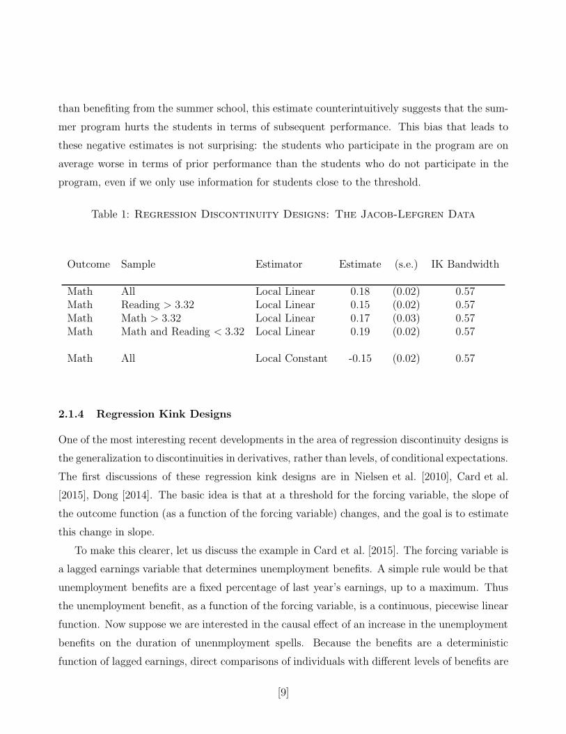
than benefiting from the summer school, this estimate counterintuitively suggests that the sum-

mer program hurts the students in terms of subsequent performance. This bias that leads to

these negative estimates is not surprising: the students who participate in the program are on

average worse in terms of prior performance than the students who do not participate in the

program, even if we only use information for students close to the threshold.

Table 1: Regression Discontinuity Designs: The Jacob-Lefgren Data

Outcome Sample Estimator Estimate (s.e.) IK Bandwidth

Math All Local Linear 0.18 (0.02) 0.57Math Reading > 3.32 Local Linear 0.15 (0.02) 0.57Math Math > 3.32 Local Linear 0.17 (0.03) 0.57Math Math and Reading < 3.32 Local Linear 0.19 (0.02) 0.57

Math All Local Constant -0.15 (0.02) 0.57

2.1.4 Regression Kink Designs

One of the most interesting recent developments in the area of regression discontinuity designs is

the generalization to discontinuities in derivatives, rather than levels, of conditional expectations.

The first discussions of these regression kink designs are in Nielsen et al. [2010], Card et al.

[2015], Dong [2014]. The basic idea is that at a threshold for the forcing variable, the slope of

the outcome function (as a function of the forcing variable) changes, and the goal is to estimate

this change in slope.

To make this clearer, let us discuss the example in Card et al. [2015]. The forcing variable is

a lagged earnings variable that determines unemployment benefits. A simple rule would be that

unemployment benefits are a fixed percentage of last year’s earnings, up to a maximum. Thus

the unemployment benefit, as a function of the forcing variable, is a continuous, piecewise linear

function. Now suppose we are interested in the causal effect of an increase in the unemployment

benefits on the duration of unenmployment spells. Because the benefits are a deterministic

function of lagged earnings, direct comparisons of individuals with different levels of benefits are

[9]

confounded by differences in lagged earnings. However, at the threshold, the relation between

benefits and lagged earnings changes. Specifically, the derivative of the benefits with respect

to lagged earnings changes. If we are willing to assume that in the absence of the kink in the

benefit system, the derivative of the expected duration would be smooth in lagged earnings,

then the change in the derivative of the expected duration with respect to lagged earnings is

informative about the relation between the expected duration and the benefit schedule, similar

to the identification in a regular regression discontinuity design.

To be more precise, suppose the benefits as a function of lagged earnings satisfy

Bi = b(Xi),

with b(x) known and continuous, with a discontinuity in the first derivative at x = c. Let b′(v)

denote the derivative, letting b′(c+) and b′(c−) denote the derivatives from the right and the

left at x = c. If the benefit schedule is piecewise linear, we would have

Bi = β0 + β1− · (Xi − c), Xi < c,

Bi = β0 + β1+ · (Xi − c), Xi ≥ c.

This relationship is deterministic, making this a sharp regression kink design. Here, as before, c

is the threshold. The forcing variable Xi is lagged earnings, Bi is the unemployment benefit that

an individual would receive. As a function of the benefits b, the logarithm of the unemployment

duration, denoted by Yi, is assumed to satisfy

Yi(b) = α + τ · ln(b) + εi.

Let g(x) = E[Yi|Xi = x] be the conditional expectation of Yi given Xi = x, with derivative g′(x).

The derivative is assumed to exist everywhere other than at x = c, where the limits from the

right and the left exist. The idea is to characterize τ as

τ =limx↓c g

′(x)− limx↑c g′(x)

limx↓c b′(x)− limx↑c b′(x).

Card et al. [2015] propose estimating τ by first estimating g(x) by local linear or local quadratic

regression around the threshold. We then divide the difference in the estimated derivative from

the right and the left by the difference in the derivatives of b(x) from the right and the left at

the threshold.

[10]

In some cases, the relationship between Bi and Xi is not deterministic, making it a fuzzy

regression kink design. In the fuzzy version of the regression kink design, the conditional expec-

tation of Bi given Xi is estimated using the same approach to get an estimate of the change in

the derivative at the threshold.

2.1.5 Summary of Recommendations

There are some specific choices to be made in regression discontinuity analyses, and here we pro-

vide our recommendations for these choices. We recommend using local linear or local quadratic

methods (see for details on the implementation Hahn et al. [2001], Porter [2003], Calonico et al.

[2014a]) rather than global polynomial methods. Gelman and Imbens [2014] present a detailed

discussion on the concerns with global polynomial methods. These local linear methods require

a bandwidth choice. We recommend the optimal bandwidth algorithms based on asymptotic ar-

guments involving local expansions discssed in Imbens and Kalyanaraman [2012], Calonico et al.

[2014a]. We also recommend carrying out supplementary analyses to assess the credibility of the

design, and in particular to test for evidence of manipulation of the forcing variable. Most impor-

tant here is the McCrary test for discontinuities in the density of the forcing variable (McCrary

[2008]), as well as tests for discontinuities in average covariate values at the threshold. We

discuss examples of these in the section on supplementary analyses (Section 3.4). We also rec-

ommend researchers to investigate external validity of the regression discontinuity estimates by

assessing the credibility of extrapolations to other subpopulations (Bertanha and Imbens [2015],

Angrist and Rokkanen [2015], Angrist and Fernandez-Val [2010], Dong and Lewbel [2015]). See

Section 2.6 for more details.

2.1.6 The Literature

Regression Discontinuity Designs have a long history, going back to work in psychology in the

fifties by Thistlewaite and Campbell [1960], but the methods did not become part of the main-

stream economics literature until the early 2000s (with Goldberger [1972, 2008] an exception).

Early applications in economics include Black [1999] Angrist and Lavy [1999], Van Der Klaauw

[2002], Lee [2008]. Recent reviews include Imbens and Lemieux [2008], Lee and Lemieux [2010],

Van Der Klaauw [2008], Skovron and Titiunik [2015]. More recently there have been many ap-

plications (e.g., Edenstein et al. [2016]) and a substantial amount of new theoretical work which

[11]

has led to substantial improvements in our understanding of these methods.

2.2 Synthetic Control Methods and Difference-In-Differences

Difference-In-Differences (DID) methods have become an important tool for empirical researchers.

In the basic setting there are two or more groups, at least one treated and one control, and we

observe (possibly different) units from all groups in two or more time periods, some prior to

the treatment and some after the treatment. The difference between the treatment and control

groups post treatment is adjusted for the difference between the two groups prior to the treat-

ment. In the simple DID case these adjustments are linear: they take the form of estimating the

average treatment effect as the difference in average outcomes post treatment minus the differ-

ence in average outcomes pre treatment. Here we discuss two important recent developments,

the synthetic control approach and the nonlinear changes-in-changes method.

2.2.1 Synthetic Control Methods

Arguably the most important innovation in the evalulation literature in the last fifteen years is

the synthetic control approach developed by Abadie et al. [2010, 2014b] and Abadie and Gardeazabal

[2003]. This method builds on difference-in-differences estimation, but uses arguably more at-

tractive comparisons to get causal effects. We discuss the basic Abadie et al. [2010] approach,

and highlight alternative choices and restrictions that may be imposed to further improve the

performance of the methods relative to difference-in-differences estimation methods.

We observe outcomes for a number of units, indexed by i = 0, . . . , N , for a number of

periods indexed by t = 1, . . . , T . There is a single unit, say unit 0, who was exposed to the

control treatment during periods 1, . . . , T0 and who received the active treatment, starting in

period T0 + 1. For ease of exposition let us focus on the case with T = T0 + 1 so there is only

a single post-treatment period. All other units are exposed to the control treatment for all

periods. The number of control units N can be as small as 1, and the number of periods T can

be as small as 2. We may also observe exogenous fixed covariates for each of the units. The

units are often aggregates of individuals, say states, or cities, or countries. We are interested in

the causal effect of the treatment for this unit, Y0T (1)− Y0T (0).

The traditional DID approach would compare the change for the treated unit (unit 0) between

periods t and T , for some t < T , to the corresponding change for some other unit. For example,

[12]

consider the classic difference-in-differences study by Card [1990]. Card is interested in the

effect of the Mariel boatlift, which brought Cubans to Miami, on the Miami labor market, and

specifically on the wages of low-skilled workers. He compares the change in the outcome of

interest, for Miami, to the corresponding change in a control city. He considers various possible

control cities, including Houston, Petersburg, Atlanta.

The synthetic control idea is to move away from using a single control unit or a simple

average of control units, and instead use a weighted average of the set of controls, with the

weights chosen so that the weighted average is similar to the treated unit in terms of lagged

outcomes and covariates. In other words, instead of choosing between Houston, Petersburg or

Atlanta, or taking a simple average of outcomes in those cities, the synthetic control approach

chooses weights λh, λp, and λa for Houston, Petersburg and Atlanta respectively, so that λh ·

Yht + λp · Ypt + λa · Yat is close to Ymt (for Miami) for the pre-treatment periods t = 1, . . . , T0,

as well as for the other pretreatment variables (e.g., Peri and Yasenov [2015]). This is a very

simple, but very useful idea. Of course, if pre-boatlift wages are higher in Houston than in

Miami, and higher in Miami than in Atlanta, it would make sense to compare Miami to the

average of Houston and Atlanta rather than to Houston or Atlanta. The simplicity of the idea,

and the obvious improvement over the standard methods, have made this a widely used method

in the short period of time since its inception.

The implementation of the synthetic control method requires a particular choice for estimat-

ing the weights. The original paper Abadie et al. [2010] restricts the weights to be non-negative

and requires them to add up to one. Let K be the dimension of the covariates Xi, and let Ω be

an arbitrary positive definite K ×K matrix. Then let λ(Ω) be the weights that solve

λ(Ω) = argminλ

(

X0 −N∑

i=1

λi ·Xi

)′

Ω

(

X0 −N∑

i=1

λi ·Xi

)

.

Abadie et al. [2010] choose the weight matrix Ω that minimizes

T0∑

t=1

(

Y0t −N∑

i=1

λi(Ω) · Yit

)2

.

If the covariatesXi consist of the vector of lagged outcomes, this estimate amounts to minimizing

T0∑

t=1

(

Y0t −

N∑

i=1

λi · Yit

)2

,

[13]

subject to the restrictions that the λi are non-negative and summ up to one.

Doudchenko and Imbens [2016] point out that one can view the question of estimating the

weights in the Abadie-Diamond-Hainmueller synthetic control method differently. Starting with

the case without covariates and only lagged outcomes, one can consider the regression function

Y0t =

N∑

i=1

λi · Yit + εt,

with T0 units and N regressors. The absence of the covariates is rarely important, as the fit

typically is driven by matching up the lagged outcomes rather than matching the covariates.

Estimating this regression by least squares is typically not possible because the number of

regressors N (the number of control units) is often larger than, or the same order of magnitude

as, the number of observations (the number of time periods T0). We therefore need to regularize

the estimates in some fashion or another. There are a couple of natural ways to do this.

Abadie et al. [2010] impose the restriction that the weights λi are non-negative and add up

to one. That often leads to a unique set of weights. However, there are alternative ways to

regularize the estimates. In fact, both the restrictions that Abadie et al. [2010] impose may

hurt performance of the model. If the unit is on the extreme end of the distribution of units,

allowing for weights that sum up to a number different from one, or allowing for negative weights

may improve the fit. We can do so by using alternative regularization methods such as best

subset regression, or LASSO (see Section 4.1.1 for a description of LASSO) where we add a

penalty proportional to the sum of the weights. Doudchenko and Imbens [2016] explore such

approaches.

2.2.2 Nonlinear Difference-in-Difference Models

A commonly noted concern with difference-in-difference methods is that functional form as-

sumptions play an important role. For example, in the extreme case with only two groups and

two periods, it is not clear whether the change over time should be modeled as the same for the

two groups in terms of levels of outcomes, or in terms of percentage changes in outcomes. If the

initial period mean outcome is different across the two groups, the two different assumptions

can give different answers in terms of both sign and magnitude. In general, a treatment might

affect both the mean and the variance of outcomes, and the impact of the treatment might vary

across individuals.

[14]

For the case where the data includes repeated cross-sections of individuals (that is, the data

include individual observations about many units within each group in two different time periods,

but the individuals can not be linked across time periods or may come from a distinct sample),

Athey and Imbens [2006] propose a non-linear difference-in-difference model which they refer to

as the changes-in-changes model that does not rely on functional form assumptions.

Modifying the notation from the last subsection, we now imagine that there are two groups,

g ∈ A,B, where group A is the control group and group B is the treatment group. There are

many individuals in each group with potential outcomes denoted Ygti(w). We observe Ygti(0)

for a sample of units in both groups when t = 1, and for group A when t = 2; we observe

Ygti(1) for group B when t = 2. Denote the distribution of the observed outcomes in group g

at time t by Fgt(·). We are interested in the distribution of treatment effects for the treatment

group in the second period, YB2i(1)− YB2i(0). Note that the distribution of YB2i(1) is directly

estimable, while the counterfactual distribution of YB2i(0) is not, so the problem boils down to

learning the distribution of YB2i(0), based on the distributions of YB1i(0), YA2i(0), and YA1i(0).

Several assumptions are required to accomplish this. First is that the potential outcome in

the absence of the treatment can be written as a monotone function of an unobservable Ui and

time: Ygti(0) = h(Ui, t). Note that the function does not depend directly on g, so that differences

across groups are attributed to differences in the distribution of Ui across groups. Second, the

function h is strictly increasing. This is not a restrictive assumption for a single time period,

but it is restrictive when we require it to hold over time, in conjunction with a third assumption,

namely that the distribution of Ui is stable over time within each group. The final assumption

is that the support of Ui for the treatment group is contained in the support of Ui for the control

group. Under these assumptions, the distribution of YB2i(0) is identified, with the formula for

the distribution given as follows:

Pr(YB2i(0) ≤ y) = FB1(F(−1)A1 (FA2(y))).

Athey and Imbens [2006] show that an estimator based on the empirical distributions of the

observed outcomes is efficient and discuss extensions to discrete outcome settings.

The nonlinear difference-in-difference model can be used for two distinct purposes. First,

the distribution is of direct interest for policy, beyond the average treatment effect. Further, a

number of authors have used this approach as a robustness check, i.e., a supplementary analysis

[15]

in the terminology of Section 3, for the results from a linear model.

2.3 Estimating Average Treatment Effects under Unconfoundedness

in Settings with Multivalued Treatments

Much of the earlier econometric literature on treatment effects focused on the case with binary

treatments. For a textbook discussion, see Imbens and Rubin [2015]. Here we discuss the results

of the more recent multi-valued treatment effect literature. In the binary treatment case, many

methods have been proposed for estimating the average treatment effect. Here we focus on

two of these methods, subclassification with regression and and matching with regression, that

have been found to be effective in the binary treatment case (Imbens and Rubin [2015]). We

discuss how these can be extended to the multi-valued treatment setting without increasing the

complexity of the estimators. In particular, the dimension reducing properties of a generalized

version of the propensity score can be maintained in the multi-valued treatment setting.

2.3.1 Set Up

To set the stage, it is useful to start with the binary treatment case. The standard set up

postulates the existence of two potential outcomes, Yi(0) and Yi(1). With the binary treatment

denoted by Wi ∈ 0, 1, the realized and observed outcome is

Y obsi = Yi(Wi) =

Yi(0) if Wi = 0,Yi(1) if Wi = 1.

In addition to the treatment indicator and the outcome we may observe a set of pretreatment

variables denoted by Xi. Following Rosenbaum and Rubin [1983a] a large literature focused on

estimation of the population average treatment effect τ = E[Yi(1) − Yi(0)], under the uncon-

foundedness assumption that

Wi ⊥⊥(

Yi(0), Yi(1))∣

∣

∣Xi.

In combination with overlap, requiring that the propensity score e(x) = pr(Wi = 1|Xi = x),

is strictly between zero and one, the researcher can estimate the population average treatment

effect by adjusting the differences in outcomes by treatment status for differences in the pre-

treatment variables:

τ = E

[

E[Y obsi |Xi,Wi = 1]− E[Y obs

i |Xi,Wi = 0]]

.

[16]

In that case many estimation strategies have been developed, relying on regression Hahn [1998],

matching Abadie and Imbens [2006], inverse propensity weighting Hirano et al. [2001], subclassi-

fication Rosenbaum and Rubin [1983a], as well as doubly robust methods Robins and Rotnitzky

[1995], Robins et al. [1995]. Rosenbaum and Rubin [1983a] established a key result that under-

lies a number of these estimation strategies: unconfoundedness implies that conditional on the

propensity score, the assignment is independent of the potential outcomes:

Wi ⊥⊥(

Yi(0), Yi(1))∣

∣

∣e(Xi).

In practice the most effective estimation methods appear to be those that combine some covari-

ance adjustment through regression with a covariate balancing method such as subclassification,

matching, or weighting based on the propensity score (Imbens and Rubin [2015]).

Substantially less attention has been paid to the case where the treatment takes on multiple

values. Exceptions include Imbens [2000], Lechner [2001], Imai and Van Dyk [2004], Cattaneo

[2010], Hirano and Imbens [2004] and Yang et al. [2016]. Let W = 0, 1, . . . , T be the set of

values for the treatment. In the multivalued treatment case, one needs to be careful in defining

estimands, and the role of the propensity score is subtly different. One natural set of estimands

is the average treatment effect if all units were switched from treatment level w1 to treatment

level w2:

τw1,w2= E[Yi(w2)− Yi(w1)]. (2.1)

To estimate estimands corresponding to uniform policies such as (2.1), it is not sufficient to

take all the units with treatment levels w1 or w2 and use methods for estimating treatment

effects in a binary setting. The latter strategy would lead to an estimate of τ ′w1,w2= E[Yi(w2)−

Yi(w1)|Wi ∈ w1, w2], which differs in general from τw1,w2because of the conditioning. Focusing

on unconditional average treatment effects like τw1,w2maintains transitivity: τw1,w2

+ τw2,w3=

τw1,w3, which would not necessarily be the case for τ ′w1,w2

. There are other possible estimands,

but we do not discuss alternatives here.

A key first step is to note that this estimand can be written as the difference in two marginal

expectations: τw1,w2= E[Yi(w2)] − E[Yi(w1)], and that therefore identification of marginal ex-

pectations such as E[Yi(w)] is sufficient for identification of average treatment effects.

[17]

Now suppose that a generalized version of unconfoundedness holds:

Wi ⊥⊥(

Yi(0), Yi(1), . . . , Yi(T ))∣

∣

∣Xi.

There is no scalar function of the covariates that maintains this conditional independence re-

lation. In fact, with T treatment levels one would need to condition on T − 1 functions of the

covariates to make this conditional independence hold. However, unconfoundedness is in fact

not required to enjoy the benefits of the dimension-reducing property of the propensity score.

Imbens [2000] introduces a concept, called weak unconfoundedness, which requires only that the

indicator for receiving a particular level of the treatment and the potential outcome for that

treatment level are conditionally independent:

1Wi=w ⊥⊥ Yi(w)∣

∣

∣Xi, for all w ∈ 0, 1, . . . , T.

Imbens [2000] shows that weak uncnfoundedness implies similar dimension reduction proper-

ties as are available in the binary treatment case. He further introduced the concept of the

generalized propensity score:

r(w, x) = pr(Wi = w|Xi = x).

Weak unconfoundedness implies that, for all w, it is sufficient for the removal of systematic

biases to condition on the generalized propensity score for that particular treatment level:

1Wi=w ⊥⊥ Yi(w)∣

∣

∣r(w,Xi).

This in turn can be used to develop matching or propensity score subclassification strategies as

outlined in Yang et al. [2016]. This approach relies on the equality E[Yi(w)] = E

[

E[Y obsi |Xi,Wi =

w]]

. As shown in Yang et al. [2016], it follows from weak unconfoundedness that

E[Yi(w)] = E

[

E[Y obsi |r(w,Xi),Wi = w]

]

.

To estimate E[Yi(w)], divide the sample into J sublasses based on the value of r(w,Xi), with

Bi ∈ 1, . . . , J denoting the subclass. We estimate µj(w) = E[Yi(w)|Bi = j] as the average

of the outcomes for units with Wi = w and Bi = j. Given those estimates, we estimate

µ(w) = E[Yi(w)] as a weighted average of the µj(w), with weights equal to the fraction of units

[18]

in subclass j. The idea is not to find subsets of the covariate space where we can interpret the

difference in average outcomes by all treatment levels as estimates of causal effects. Instead we

find subsets where we can estimate the marginal average outcome for a particular treatment

level as the conditional average for units with that treatment level, one treatment level at a

time. This opens up the way for using matching and other propensity score methods developed

for the case with binary treatments in settings with multivalued treatments, irrespective of the

number of treatment levels.

A separate literature has gone beyond the multi-valued treatment setting to look at dy-

namic treatment regimes. With few exceptions most of these studies appear in the biostatistical

literature: see Hernan and Robins [2006] for a general discussion.

2.4 Causal Effects in Networks and Social Interactions

An important area that has seen much novel work in recent years is that on peer effects and

causal effects in networks. Compared to the literature on estimating average causal effects

unconfoundedness without interference, the literature has not focused on a single setting; rather,

there are many problems and settings with interesting questions. Here, we will discuss some

of the settings and some of the progress that has been made. However, this review will be

brief, and incomplete, because this continues to be a very active area, with work ranging from

econometrics (Manski [1993]) to economic theory (Jackson [2010]).

In general, the questions in this literature focus on causal effects in settings where units, often

individuals, interact in a way that makes the no-interference or sutva (Rosenbaum and Rubin

[1983a], Imbens and Rubin [2015]) assumptions that are routinely made in the treatment effect

literature implausible. Settings of interest include those where the possible interference is simply

a nuisance, and the interest continuous to be in causal effects of treatments assigned to a

particular unit on the outcomes for that unit. There are also settings where the interest is in

the magnitude of the interactions, or peer effects, that is, in the effects of changing treatments

for one unit on the outcomes of other units. There are settings where the network (that is,

the set of links connecting the individuals) is fixed exogenously, and some where the network

itself is the result of a possibly complex set of choices by individuals, possibly dynamic and

possibly affected by treatments. There are settings where the population can be partitioned into

subpopulations with all units within a subpopulation connected, as, for example, in classroom

[19]

settings (e.g., Manski [1993], Carrell et al. [2013]), workers in a labor market (Crepon et al.

[2013]) or roommates in college (Sacerdote [2001]), or with general networks, where friends of

friends are not necessarily friends themselves (Christakis and Fowler [2007]). Sometimes it is

more reasonable to think of many disconnected networks, where distributional approximations

rely on the number of networks getting large, versus a single connected network such as Facebook.

It maybe reasonable in some cases to think of the links as undirected (symmetric), and in others

as directed. These links can be binary, with links either present or not, or contain links of

different strengths. This large set of scenarios has led to the literature becoming somewhat

fractured and unwieldy. We will only touch on a subset of these problems in this review.

2.4.1 Models for Peer Effects

Before considering estimation strategies, it is useful to begin by considering models of the out-

comes in a setting with peer effects. Such models have been proposed in the literature. A

seminal paper in the econometric literature is Manski’s linear-in-means model (Manski [1993],

Bramoulle and Fortin [2009], Goldsmith-Pinkham and Imbens [2013]). Manski’s original paper

focuses on the setting where the population is partioned into groups (e.g., classrooms), and peer

effects are constant within the groups. The basic model specification is

Yi = β0 + βY · Y i + β ′XXi + β ′

XX i + β ′

ZZi + εi,

where i indexes the individual. Here Yi is the outcome for individual i, Y i is the average outcome

for individuals in the peer group for individual i, Xi is a set of exogenous characteristics of

individual i, X i is the average value of the characteristics in individual i’s peer group, and Zi

are group characteristics that are constant for all individuals in the same peer group. Manski

considers three types of peer effects. Outcomes for individuals in the same group may be

correlated because of a shared environment. These effects are called correlated peer effects, and

captured by the coefficient on Zi. Next are the exogenous peer effects, captured by the coefficient

on the group average Xi of the exogenous variables. The third type is the endogenous peer

effect, captured by the coefficient on the group average outcomes Y i. Manski concludes that

identification of these effects, even in the linear model setting, relies on very strong assumptions

and is unrealistic in many settings. In subsequent empirical work, researchers have often ruled

out some of these effects in order to identify others.

[20]

Graham [2008] focuses on a setting very similar to that of Manski’s linear-in-means model.

He considers restrictions on the covariance matrix within peer groups implied by the model

assuming homoskedasticity at the individual level. Bramoulle and Fortin [2009] allows for a more

general network configuration than Manski, and investigate the benefits of such configurations

for identification in the Manski-style linear-in-means model. Hudgens and Halloran [2008] start

closer to the Rubin Causal Model or potential outcome setup. Like Manski they focus on a

setting with a partitioned network. Following the treatment effect literature they focus primarily

on the case with a binary treatment. Let Wi denote the treatment for individual i, and let Wi

denote the vector of treatments for the peer group for individual i. The starting point in the

Hudgens and Halloran [2008] set up is the potential outcome Yi(w), with restrictions placed on

the dependence of the potential outcomes on the full treatment vector w. Aronow and Samii

[2013] allow for general networks and peer effects, investigating the identifying power from

randomization.

2.4.2 Models for Network Formation

Another part of the literature has focused on developing models for network formation. Such

models are of interest in their own right, but they are also important for deriving asymptotic

approximations based on large samples. Such approximations require the researcher to specify

in what way the expanding sample would be similar to or different from the current sample. For

example, it would require the researcher to be specific in the way the additional units would be

linked to current units or other new units.

There is a wide range of models considered, with some models relying more heavily on opti-

mizing behavior of individuals, and others using more statistical models. See Goldsmith-Pinkham and Imbens

[2013], Christakis et al. [2010], Mele [2013], Jackson [2010], Jackson and Wolinsky [1996] for

such network models in economics, and Holland and Leinhardt [1981] for statistical models.

Chandrasekhar and Jackson develops a model for network formation and develops a correspond-

ing central limit theorem in the presence of correlation induced by network links. Chandrasekhar

surveys the econometrics of network formation.

[21]

2.4.3 Exact Tests for Interactions

One challenge in testing hypotheses about peer effects using methods based on standard asymp-

totic theory is that when individuals interact (e.g., in a network), it is not clear how interactions

among individuals would change as the network grows. Such a theory would require a model

for network formation, as discussed in the last subsection. This motivates an approach that

allows us to test hypotheses without invoking large sample properties of test statistics (such as

asymptotic normality). Instead, the distributions of the test statistics are based on the random

assignments of the treatment, that is, the properties of the tests are based on randomization in-

ference. In randomization inference, we approximate the distribution of the test statistic under

the null hypothesis by re-calculating the test statistic under a large number of alternative (hypo-

thetical) treatment assignment vectors, where the alternative treatment assignment vectors are

drawn from the randomization distribution. For example, if units were independently assigned

to treatment status with probability p, we re-draw hypothetical assignment vectors with each

unit assigned to treatment with probability p. Of course, re-calculating the test statistic requires

knowing the values of units’ outcomes. The randomization inference approach is easily applied

if the null hypothesis of interest is “sharp”: that is, the null hypothesis specifies what outcomes

would be under all possible treatment assignment vectors. If the null hypothesis is that the

treatment has no effect on any units, this null is sharp: we can infer what outcomes would have

been under alternative treatment assignment vectors, in in particular, outcomes would be the

same as the realized outcomes under the realized treatment vector.

More generally, however, randomization inference for tests for peer effects is more compli-

cated than in settings without peer effects because the null hypotheses are often not sharp.

Aronow [2012], Athey et al. [2015] develop methods for calculating exact p-values for general

null hypotheses on causal effects in a single connected network, allowing for peer effects. The

basic case Aronow [2012], Athey et al. [2015] consider is that where the null hypothesis rules out

peer effects but allows for direct (own) effects of a binary treatment assigned randomly at the

individual level. Given that direct effects are not specified under the null, individual outcomes

are not known under alternative treatment assignment vectors, and so the null is not sharp. To

address this problem, Athey et al. [2015] introduce the notion of an artificial experiment that

differs from the actual experiment. In the artificial experiment, some units have their treatment

[22]

assignments held fixed, and we randomize over the remaining units. Thus, the randomization dis-

tribution is replaced by a conditional randomization distribution, where treatment assignments

of some units are re-randomized conditional on the assignment of other units. By focusing on

the conditional assignment given a subset of the overall space of assignments, and by focusing on

outcomes for a subset of the units in the original experiment, they create an artificial experiment

where the original null hypothesis that was not sharp in the original experiment is now sharp.

To be specific, the artificial experiments starts by designating an arbitrary set of units to be

focal. The test statistics considered depend only on outcomes for these focal units. Given the

focal units, the set of assignments that, under the null hypothesis of interest, does not change

the outcomes for the focal units is derived. The exact distribution of the test statistic can then

be inferred for such test statistics under that conditional randomization distribution under the

null hypothesis considered.

Athey et al. [2015] extend this idea to a large class of null hypotheses. This class includes

hypotheses restricting higher order peer effects (peer effects from friends-of-friends) while allow-

ing for the presence of peer effects from friends. It also includes hypotheses about the validity of

sparsification of a dense network, where the question concerns peer effects of friends according

to the pre-sparsified network while allowing for peer effects of the sparsified network. Finally,

the class also includes null hypotheses concerning the exchangeability of peers. In many models

peer effects are restricted so that all peers have equal effects on an individual’s outcome. It

may be more realistic to allow effects of highly connected individuals, or closer friends, to be be

different from those of less connected or more distant friends. Such hypotheses can be tested in

this framework.

2.5 Randomization Inference and Causal Regressions

In recent empirical work, data from randomized experiments are often analyzed using conven-

tional regression methods. Some researchers have raised concerns with the regression approach in

small samples (Freedman [2006, 2008], Young [2015], Athey and Imbens [2016], Imbens and Rubin

[2015]), but generally such analyses are justified at least in large samples, even in settings with

many covariates (Bloniarz et al. [2016], Du et al. [2016]). There is an alternative approach to

estimation and inference, however, that does not rely on large sample approximations, using

approximations for the distribution of estimators induced by randomization. Such methods,

[23]

which go back to Fisher [1925, 1935], Neyman [1923/1990, 1935], clarify how the act of random-

ization allows for the testing for the presence of treatment effects and the unbiased estimation of

average treatment effects. Traditionally these methods have not been used much in economics.

However, recently there has been some renewed interest in such methods. See for example

Imbens and Rosenbaum [2005], Young [2015], Athey and Imbens [2016]). In completely ran-

domized experiments these methods are often straightforward, although even there analyses

involving covariates can be more complicated.

However, the value of the randomization perspective extends well beyond the analysis of

actual experiments. It can shed light on the interpretation of observational studies and the

complications arising from finite population inference and clustering. Here we discuss some of

these issues and more generally provide an explicitly causal perspective on linear regression.

Most textbook discussions of regression specify the regression function in terms of a dependent

variable, a number of explanatory variables, and an unobserved component, the latter often

referred to as the error term:

Yi = β0 +

K∑

k=1

βk ·Xik + εi.

Often the assumption is made that in the population the units are randomly sampled from,

the unobserved component εi is independent of, or uncorrelated with, the regressors Xik. The

regression coefficients are then estimated by least squares, with the uncertainty in the estimates

interpreted as sampling uncertainty induced by random sampling from the large population.

This approach works well in many cases. In analyses using data from the public use surveys

such as the Current Population Survey or the Panel Study of Income Dynamics it is natural

to view the sample at hand as a random sample from a large population. In other cases this

perspective is not so natural, with the sample not drawn from a well-defined population. This

includes convenience samples, as well as settings where we observe all units in the population.

In those cases it is helpful to take an explictly causal perspective. This perspective also clarifies

how the assumptions underlying identification of causal effects relate to the assumptions often

made in least squares approaches to estimation.

Let us separate the covariates Xi into a subset of causal variables Wi and the remainder,

viewed as fixed characteristics of the units. For example, in a wage regression the causal variable

may be years of education and the characteristics may include sex, age, and parental background.

[24]

Using the potential outcomes perspective we can interpret Yi(w) as the outcome corresponding to

a level of the treatment w for unit or individual i. Now suppose that for all units i the function

Yi(·) is linear in in its argument, with a common slope coefficient, but a variable intercept,

Yi(w) = Yi(0) + βW · w. Now write Yi(0), the outcome for unit i given treatment level 0 as

Yi(0) = β0 + β ′ZZi + εi,

where β0 and βZ are the population best linear predictor coefficients. This representation of

Yi(0) is purely definitional and does not require assumptions on the population. Then we can

write the model as

Yi(w) = β0 + βW · w + β ′ZZi + εi,

and the realized outcome as

Yi = β0 + βW ·Wi + β ′ZZi + εi.

Now we can investigate the properties of the least squares estimator βW for βW , where the

distribution of βW is generated by the assignment mechanism for the Wi. In the simple case

where there are no characteristics Zi and the cause Wi is a binary indicator, the assumption

that the cause is completely randomly assigned leads to the conventional Eicker-Huber-White

standard errors (Eicker [1967], Huber [1967], White [1980]). Thus, in that case viewing the

randomness as arising from the assignment of the causes rather than as sampling uncertainty

provides a coherent way of interpreting the uncertainty.

This extends very easily to the case where Wi is binary and completely randomly as-

signed but there are other regressors included in the regression function. As Lin [2013] and

Imbens and Rubin [2015] show there is no need for assumptions about the relation of those

regressors to the outcome, as long as the cause Wi is randomly assigned. Abadie et al. [2014a]

extend this to the case where the cause is multivalued, possibly continuous, and the charac-

teristics Zi are allowed to be generally correlated with the cause Wi. Aronow and Samii [2013]

discuss the interpretation of the regression estimates in a causal framework. Abadie et al. [2016]

discuss extensions to settings with clustering where the need for clustering adjustments in stan-

dard errors arises from the clustered assignment of the treatment rather than through clustered

sampling.

[25]

2.6 External Validity

One concern that has been raised in many studies of causal effects is that of external validity.

Even if a causal study is done carefully, either in analysis or by design, so that the internal

validity of such a study is high, there is often little guarantee that the causal effects are valid

for populations or settings other than those studied. This concern has been raised particularly

forcefully in experimental studies where the internal validity is guaranteed by design. See for

example the discussion in Deaton [2010], Imbens [2010] and Manski [2013]. Traditionally, there

has been much emphasis on internal validity in studies of causal effects, with some arguing for

the primacy of internal validity. Some have argued that without internal validity, little can be

learned from a study (Shadish et al. [2002], Imbens [2015a]). Recently, however, Deaton [2010],

Manski [2013], Banerjee et al. [2016] have argued that external validity should receive more

emphasis.

Some recent work has taken concerns with external validity more seriously, proposing a

variety of approaches that directly allow researchers to assess the external validity of esti-

mators for causal effects. A leading example concerns settings with instrumental variables

with heterogenous treatment effects (e.g., Angrist [2004], Angrist and Fernandez-Val [2010],

Dong and Lewbel [2015], Angrist and Rokkanen [2015], Bertanha and Imbens [2015], Kowalski

[2015], Brinch et al. [2015]). In the modern literature with heterogenous treatment effects the

instrumental variables estimator is interpreted as an estimator of the local average treatment

effect, the average effect of the treatment for the compliers, that is, individuals whose treatment

status is affected by the instrument. In this setting, the focus has been on whether the instru-

mental variables estimates are relevant for the entire sample, that is, have external validity, or

only have local validity for the complier subpopulation.

In that context, Angrist [2004] suggests testing whether the difference in average outcomes

for always-takers and never-takers is equal to the average effect for compliers. In this context,

a Hausman test [Hausman, 1978] for equality of the ordinary least squares estimate and an

instrumental variables estimate can be interpreted as testing whether the average treatment

effect is equal to the local average treatment effect; of course, the ordinary least squares es-

timate only has that interpretation if unconfoundedness holds. Bertanha and Imbens [2015]

suggest testing a combination of two equalities, first that the average outcome for untreated

[26]

compliers is equal to the average outcome for never-takers, and second, that the average out-

come for treated compliers is equal to the average outcome for always-takers. This turns out

to be equivalent to testing both the null hypothesis suggested by Angrist [2004] and the Haus-

man null. Angrist and Fernandez-Val [2010] consider extrapolating local average treatment

effects by exploiting the presence of other exogenous covariates. The key assumption in the

Angrist and Fernandez-Val [2010] approach, “conditional effect ignorability,” is that conditional

on these additional covariates the average effect for compliers is identical to the average effect

for never-takers and always-takers.

In the context of regression discontinuity designs, and especially in the fuzzy regression

discontinuity setting, the concerns about external validity are especially salient. In that set-

ting the estimates are in principle valid only for individuals with values of the forcing variable

equal to, or close to, the threshold at which the probability of receipt of the treatment changes

discontinuously. There have been a number of approaches to assess the plausibility of gener-

alizing those local estimates to other parts of the population. The focus and the applicability

of the various methods to assess external validity varies. Some of them apply to both sharp

and fuzzy regression discontinuity designs, and some apply only to fuzzy designs. Some require

the presence of additional exogenous covariates, and others rely only on the presence of the

forcing variable. Dong and Lewbel [2015] observe that in general, in regression discontinuity

designs with a continuous forcing variable, one can estimate the magnitude of the discontinuity

as well as the magnitude of the change in the first derivative of the regression function, or even

higher order derivatives. Under assumptions about the smoothness of the two conditional mean

functions, knowing the higher order derivatives allows one to extrapolate away from values of

the forcing variable close to the threshold. This method apply both in the sharp and in the

fuzzy regression discontinuity design. It does not require the presence of additional covariates.

In another approach, Angrist and Rokkanen [2015] do require the presence of additional ex-

ogenous covariates. They suggest testing whether whether conditional on these covariates, the

correlation between the forcing variable and the outcome vanishes. This would imply that the

assignment can be thought of as unconfounded conditional on the additional covariates. Thus

it would allow for extrapolation away from the threshold. Like the Dong-Lewbel approach, the

Angrist-Rokkanen methods apply both in the case of sharp and fuzzy regression discontinuity

designs. Finally, Bertanha and Imbens [2015] propose an approach requiring a fuzzy regression

[27]

discontinuity design. They suggest testing for continuity of the conditional expectation of the

outcome conditional on the treatment and the forcing variable, at the threshold, adjusted for

differences in the covariates.

2.7 Leveraging Experiments

Randomized experiments are the most credible design to learn about causal effects. However,

in practice there are often reasons that researchers cannot conduct randomized experiments to

answer the causal questions of interest. They may be expensive, or they may take too long to

give the researcher the answers that are needed now to make decisions, or there may be ethical

objections to experimentation. As a result, we often rely on a combination of experimental

results and observational studies to make inferences and decisions about a wide range of ques-

tions. In those cases we wish to exploit the benefits of the experimental results, in particular

the high degree of internal validity, in combination with the external validity and precision from

large scale representative observational studies. At an abstract level, the observational data

are used to estimate rich models that allow one to answer many questions, but the model is

forced to accommodate the answers from the experimental data for the limited set of questions

the latter can address. Doing so will improve the answers from the observational data without

compromising their ability to answer more questions.

Here we discuss two specific settings where experimental studies can be leveraged in combina-

tion with observational studies to provide richer answers than either of the designs could provide

on their own. In both cases, the interest is in the average causal effect of a binary treatment

on a primary outcome. However, in the experiment the primary outcome was not observed and

so one cannot directly estimate the average effect of interest. Instead an intermediate outcome

was observed. In a second study, both the intermediate outcome and the primary outcome were

observed. In both studies there may be additional pretreatment variables observed and possibly

the treatment indicator.

These two examples do not exhaust the set of possible settings where researchers can leverage

experimental data more effectively, and this is likely to be an area where more research is fruitful.

[28]

2.7.1 Surrogate Variables

In the first setting, studied in Athey et al. [2016b], in the second sample the treatment indicator

is not observed. In this case researchers may wish to use the intermediate variable, denoted Si, as

a surrogate. Following Prentice [1989], Begg and Leung [2000], Frangakis and Rubin [2002], the

key condition for an intermediate variable to be a surrogate is that in the experimental sample,

conditional the surrogate and observed covariates, the (primary) outcomes and the treatment

are independent: Yi ⊥⊥ Wi|(Si, Xi). There is a long history of attempts to use intermediate

health measures in medical trials as surrogates (Prentice [1989]). The results are mixed, with

the condition often not satisfied in settings where it could be tested. However, many of these

studies use low-dimensional surrogates. In modern settings there is often a large number of

intermediate variables recorded in administrative data bases that lie on or close to the causal

path between the treatment and the primary outcome. In such cases it may be more plausible

that the full set of surrogate variables satisfies at least approximately the surrogacy condition.

For example, suppose an internet company is considering a change to the user experience on

the company’s website. They are interested in the effect of that change on the user’s engagement

with the website over a year long period. They carry out a randomized experiment over a

month, where they measure details about the user’s engagement, including the number of visits,

webpages visited, and the length of time spent on the various webpages. In addition, they may

have historical records on user characteristics including past engagement, for a large number of

users. The combination of the pretreatment variables and the surrogates may be sufficiently rich

so that conditional on the combination the primary outcome is independent of the treatment.

Given surrogacy, and given comparability of the observational and experimental sample

(which requires that the conditional distribution of the primary outcome given surrogates and

pretreatment variables is the same in the experimental and observational sample), Athey et al.

[2016b] develop two methods for estimating the average effect. The first corresponds to estimat-

ing the relation between the outcome and the surrogates in the observational data and using

that to impute the missing outcomes in the experimental sample. The second corresponds to

estimating the relation between the treatment and the surrogates in the experimental sample

and use that to impute the treatment indicator in the observational sample. They also derive

the biases from violations of the surrogacy assumption.

[29]

2.7.2 Experiments and Observational Studies

In the second setting, studied in Athey et al. [2016a], the researcher again has data from a ran-

domized experiment containing information on the treatment and the intermediate variables, as

well as pretreatment variables. In the observational study the researcher now observes the same

variables plus the primary outcome. If in the observational study unconfoundedness (selection-

on-observables) were to hold, the researcher would not need the experimental sample, and could

simply estimate the average effect of the treatment on the primary outcome by adjusting for dif-

ferences between treated and control units in pretreatment variables. However, one can compare

the estimates of the average effect on the intermediate outcomes based on the observational sam-

ple, after adjusting for pretreatment variables, with those from the experimental sample. The

latter are known to be consistent, and so if one finds substantial and statistically significant

differences, unconfoundedness need not hold. For that case Athey et al. [2016a] develop meth-

ods for adjusting for selection on unobservables exploiting the observations on the intermediate

variables.

2.7.3 Multiple Experiments

An issue that has not received as much attention, but provides fertile ground for future work

concerns the use of multiple experiments. Consider a setting where a number of experiments were

conducted. The experiments may vary in terms of the population that the sample is drawn from,

or in the exact nature of the treatments included. The researcher may be interested in combining

these experiments to obtain more efficient estimates, predicting the effect of a treatment in

another population, or estimating the effect of a treatment with different characteristics. Such

inferences are not validated by the design of the experiments, but the experiments are important

in making such inferences more credible. These issues are related to external validity concerns,

but include more general efforts to decompose experimentally estimated effects into components

that can inform decisions on related treatments. In the treatment effect literature aspects of

these problems have been studied in Hotz et al. [2005], Imbens [2010], Allcott [2015]. They have

also received some attention in the literature on structural modeling, where the experimental

data are used to anchor aspects of the structural model, e.g., Todd and Wolpin [2003].

[30]

3 Supplementary Analyses

One common feature of much of the empirical work in the causal literature is the use of what

we call here supplementary analyses. We want to contrast supplementary analyses with primary

analyses whose focus is on point estimates of the primary estimands and standard errors thereof.

Instead, the point of the supplementary analyses is to shed light on the credibility of the primary

analyses. They are intended to probe the identification strategy underlying the primary analyses.

The results of these supplementary analyses is not to end up with a better estimate of the effect

of primary interest. The goal is also not to directly select among competing statistical models.

Rather, the results of the supplementary analyses either enhance the credibility of the primary

analyses or cast doubts on them, without necessarily suggesting alternatives to these primary

analyses (although sometimes they may). The supplementary analyses are often based on careful

and creative examinations of the identification strategy. Although at first glance, this creativity

may appear application-specific, in this section we try to highlight some common themes.

In general, the assumptions behind the identification strategy often have implications for the

data beyond those exploited in the primary analyses, and these implications are the focus of

the supplementary analyses. The supplementary analyses can take on a variety of forms, and

we are currently not aware of a comprehensive survey to date. Here we discuss some examples

from the empirical and theoretical literatures and draw some general conclusions in the hope of

providing some guidance for future work. This is a very active literature, both in theoretical and

empirical studies, and it is likely that the development of these methods will continue rapidly.

The assumptions underlying identification strategies can typically be stated without reference

to functional form assumptions or estimation strategies. For example, unconfoundedness is a

conditional independence assumption. There are variety of estimation strategies that exploit the

unconfoundedness assumption. Supplementary analyses may attempt to establish the credibility

of the underlying independence assumption; or, they may jointly establish the credibility of the

underlying assumption and the specific estimation approach used for the primary analysis.

In Section 3.1 we discuss one of the most common forms of supplementary analyses, placebo

analysis, where pseudo causal effects are estimated that are known to be equal to zero. In Section

3.2 we discuss sensitivity and robustness analyses that assess how much estimates of the primary

estimands can change if we weaken the critical assumptions underlying the primary analyses.

[31]

In Section 3.3 we discuss some recent work on understanding the identification of key model

estimates by linking model parameters to summary statistics of the data. In Section 3.4 we disuss

a particular supplementary analysis that is specific to regression discontinuity analyses. In this

case the focus is on the continuity of the density of an exogenous variable, with a discontinuity

as the threshold for the regression discontinuity analyses evidence of manipulation of the forcing

variable.

3.1 Placebo Analyses

The most widely used of the supplementary analyses is what is often referred to as a placebo

analysis. In this case the researcher replicates the primary analysis with the outcome replaced

by a pseudo outcome that is known not to be affected by the treatment. Thus, the true value

of the estimand for this pseudo outcome is zero, and the goal of the supplementary analysis is

to assess whether the adjustment methods employed in the primary analysis when applied to

the pseudo outcome lead to estimates that are close to zero, taking into account the statistical

uncertainty. Here we discuss some settings where such analyses, in different forms, have been

applied, and provide some general guidance. Although these analyses often take the form of

estimating an average treatment effect and testing whether that is equal to zero, underlying the

approach is often conditional independence relation. In this review we highlight the fact that

there is typically more to be tested than simply a single average treatment effect.

3.1.1 Lagged Outcomes

One type of placebo test relies on treating lagged outcomes as pseudo outcomes. Consider, for

example, the lottery data set assembled by Imbens et al. [2001], which studies participants in

the Massachusetts state lottery. The treatment of interest is an indicator for winning a big prize

in the lottery (with these prizes paid out over a twenty year period), with the control group

consisting of individuals who won one small, one-time prizes. The estimates of the average

treatment effect rely on an unconfoundedness assumption, namely that the lottery prize is as

good as randomly assigned after taking out associations with some pre-lottery variables:

Wi ⊥⊥(

Yi(0), Yi(1))∣

∣

∣Xi. (3.1)

[32]

Table 2: Lagged as Pseudo-Outcomes in the Lottery Data

Outcome est (s.e.)

Pseudo Outcome: Y−1,i -0.53 (0.78)

Actual Outcome: Y obsi -5.74 (1.40)

The pre-treatment variables include six years of lagged earnings as well as six individual charac-

teristics (including education measures and gender). Unconfoundedness is plausible here because

which ticket wins the lottery is random, but because of a 50% response rate, as well as differences

in the rate at which individuals buy lottery tickets, there is no guarantee that this assumption

holds. To assess the assumption it is useful to estimate the same regression function with pre-

lottery earnings as the outcome, and the indicator for winning on the right hand side with the

same set of additional exogenous covariates. Formally, we partition the vector of covariates Xi

into two parts, a (scalar) pseudo outcome, denoted by Xpi , and the remainder, denoted by Xr

i ,

so that Xi = (Xpi , X

ri ). We can then test the conditional independence relation

Wi ⊥⊥ Xpi

∣

∣

∣Xr

i . (3.2)

Why is testing this conditional independence relation relevant for assessing unconfoundedness

in (3.1)? There are two conceptual steps. One is that the pseudo outcome Xpi is viewed as

a proxy for one or both of the potential outcomes. Second, it relies on the notion that if

unconfoundedness holds given the full set of pretreatment variables Xi, it is plausible that it

also holds given the subset Xri . In the lottery application, taking Xp

i to be earnings in the

year prior to winning or not, both steps appear plausible. Results for this analysis are in Table

2. Using the actual outcome we estimate that winning the lottery (with on average a $20,000

yearly prize), reduces average post-lottery earnings by $5,740, with a standard error of $1,400.

Using the pseudo outcome we obtain an estimate of minus $530, with a standard error of $780.

In Table 3, we take this one step further by testing the conditional independence relation

in (3.2) more fully. We do this by testing the null of no average difference for two functions

of the pseudo-outcome, namely the actual level and an indicator for the pseudo-outcome being

[33]

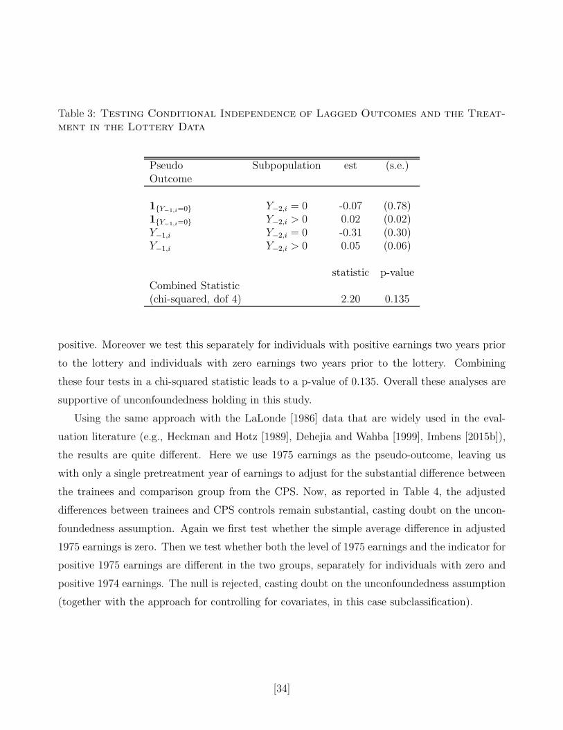
Table 3: Testing Conditional Independence of Lagged Outcomes and the Treat-

ment in the Lottery Data

Pseudo Subpopulation est (s.e.)Outcome

1Y−1,i=0 Y−2,i = 0 -0.07 (0.78)

1Y−1,i=0 Y−2,i > 0 0.02 (0.02)

Y−1,i Y−2,i = 0 -0.31 (0.30)Y−1,i Y−2,i > 0 0.05 (0.06)

statistic p-valueCombined Statistic(chi-squared, dof 4) 2.20 0.135

positive. Moreover we test this separately for individuals with positive earnings two years prior

to the lottery and individuals with zero earnings two years prior to the lottery. Combining

these four tests in a chi-squared statistic leads to a p-value of 0.135. Overall these analyses are

supportive of unconfoundedness holding in this study.

Using the same approach with the LaLonde [1986] data that are widely used in the eval-

uation literature (e.g., Heckman and Hotz [1989], Dehejia and Wahba [1999], Imbens [2015b]),

the results are quite different. Here we use 1975 earnings as the pseudo-outcome, leaving us

with only a single pretreatment year of earnings to adjust for the substantial difference between

the trainees and comparison group from the CPS. Now, as reported in Table 4, the adjusted

differences between trainees and CPS controls remain substantial, casting doubt on the uncon-

foundedness assumption. Again we first test whether the simple average difference in adjusted

1975 earnings is zero. Then we test whether both the level of 1975 earnings and the indicator for

positive 1975 earnings are different in the two groups, separately for individuals with zero and

positive 1974 earnings. The null is rejected, casting doubt on the unconfoundedness assumption

(together with the approach for controlling for covariates, in this case subclassification).

[34]

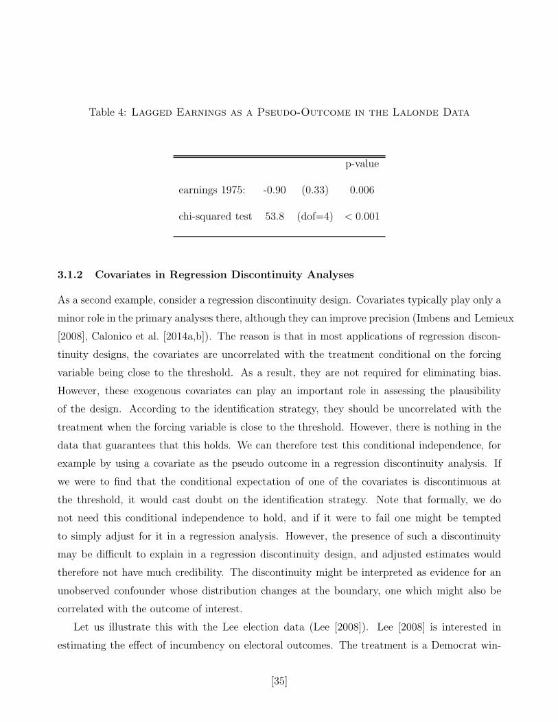
Table 4: Lagged Earnings as a Pseudo-Outcome in the Lalonde Data

p-value

earnings 1975: -0.90 (0.33) 0.006

chi-squared test 53.8 (dof=4) < 0.001

3.1.2 Covariates in Regression Discontinuity Analyses

As a second example, consider a regression discontinuity design. Covariates typically play only a

minor role in the primary analyses there, although they can improve precision (Imbens and Lemieux

[2008], Calonico et al. [2014a,b]). The reason is that in most applications of regression discon-

tinuity designs, the covariates are uncorrelated with the treatment conditional on the forcing

variable being close to the threshold. As a result, they are not required for eliminating bias.

However, these exogenous covariates can play an important role in assessing the plausibility

of the design. According to the identification strategy, they should be uncorrelated with the

treatment when the forcing variable is close to the threshold. However, there is nothing in the

data that guarantees that this holds. We can therefore test this conditional independence, for

example by using a covariate as the pseudo outcome in a regression discontinuity analysis. If

we were to find that the conditional expectation of one of the covariates is discontinuous at

the threshold, it would cast doubt on the identification strategy. Note that formally, we do

not need this conditional independence to hold, and if it were to fail one might be tempted

to simply adjust for it in a regression analysis. However, the presence of such a discontinuity

may be difficult to explain in a regression discontinuity design, and adjusted estimates would

therefore not have much credibility. The discontinuity might be interpreted as evidence for an

unobserved confounder whose distribution changes at the boundary, one which might also be

correlated with the outcome of interest.

Let us illustrate this with the Lee election data (Lee [2008]). Lee [2008] is interested in

estimating the effect of incumbency on electoral outcomes. The treatment is a Democrat win-

[35]

ning a congressional election, and the forcing variable is the Democratic vote share minus the

Republication vote share in the current election. We look at an indicator for winning the next

election as the outcome. As a pretreatment variable, we consider an indicator for winning the

previous election to the one that defines the forcing variable. Table 5 presents the results, based

on the Imbens-Kalyanaraman bandwidth, where we use local linear regression (weighted with a

triangular kernel to account for boundary issues). The estimates for the actual outcome (win-

Table 5: Winning a Previous Election as a Pseudo-Outcome in Election Data

Democrat Winning Next Election 0.43 (0.03) 0.26

Democrat Winning Previous Election 0.03 (0.03) 0.19

ning the next election) are substantially larger than those for the pseudo outcome (winning the

previous election), where we cannot reject the null hypothesis that the effect on the pseudo

outcome is zero.

3.1.3 Multiple Control Groups

Another example of the use of placebo regressions is Rosenbaum et al. [1987] (see also Heckman and Hotz

[1989], Imbens and Rubin [2015]). Rosenbaum et al. [1987] is interested in the causal effect of a

binary treatment and focuses on a setting with multiple comparison groups. There is no strong

reason to believe that one of the comparison groups is superior to another. Rosenbaum et al.

[1987] proposes testing equality of the average outcomes in the two comparison groups after

adjusting for pretreatment variables. If one finds that there are substantial differences left after

such adjustments, it shows that at least one of the comparison groups is not valid, which makes

the use of either of them less credible. In applications to evaluations of labor market programs

one might implement such methods by comparing individuals who are eligible but choose not to

participate, to individuals who are not eligible. The biases from evaluations based on the first

[36]

control group might correspond to differences in motivation, whereas evaluations based on the

second control group could be biased because of direct associations between eligibility criteria

and outcomes.

Note that one can also exploit the presence of multiple control groups by comparing esti-

mates of the actual treatment effect based on one comparison group to that based on a second

comparison group. Although this approach seems appealing at first glance, it is in fact less

effective than direct comparisons of the two comparison groups because comparing treatment

effect estimates involves the data for the treatment group, whose outcomes are not relevant for

the hypothesis at hand.

3.2 Robustness and Sensitivity

Another form of supplementary analyses focuses on sensitivity and robustness measures. The

classical frequentist statistical paradigm suggests that a researcher specifies a single statistical

model. The researcher then estimates this model on the data, and reports estimates and standard

errors. The standard errors and the corresponding confidence intervals are valid given under

the assumption that the model is correctly specified, and estimated only once. This is of course

far from common practice, as pointed out, for example, in Leamer [1978, 1983]. In practice

researcher consider many specifications and perform various specification tests before settling

on a preferred model. Not all the intermediate estimation results and tests are reported.

A common practice in modern empirical work is to present in the final paper estimates of the

preferred specification of the model, in combination with assessments of the robustness of the

findings from this preferred specification. These alternative specifications are not intended to be

interpreted as statistical tests of the validity of the preferred model, rather they are intended to

convey that the substantive results of the preferred specification are not sensitive to some of the

choices in that specification. These alternative specifications may involve different functional

forms of the regression function, or different ways of controlling for differences in subpopulations.

Recently there has been some work trying to make these efforts at assessing robustness more

systematic.

Athey and Imbens [2015] propose an approach to this problem. We can illustrate the ap-

proach in the context of regression analyses, although it can also be applied to more complex

nonlinear or structural models. In the regression context, suppose that the object of interest is

[37]

a particular regression coefficient that has an interpretation as a causal effect. For example, in

the preferred specification

E[Yi|Xi, Zi] = β0 + βW ·Wi + β ′ZZi,

the interest may be in βW , the coefficient on Wi. They then suggest considering a set of different

specifications based on splitting the sample into two subsamples, with Xi ∈ 0, 1 denoting the

subsample, and in each case estimating

E[Yi|Wi, Zi, Zi = z] = β0x + βWx ·Wi + β ′ZxZi.

The original causal effect is then estimated as βW = X · βW1 + (1 − X) · βW0. If the original

model is correct, the augmented model still leads to a consistent estimator for the estimand.

Athey and Imbens [2015] suggest splitting the original sample once for each of the elements of the

original covariate vector Zi, and splitting at a threshold that optimizes fit by minimizing the sum

of squared residuals. Note that the focus is not on finding an alternative specification that may

provide a better fit; rather, it is on assessing whether the estimate in the original specification

is robust to a range of alternative specifications. They suggest reporting the standard deviation

of the βW over the set of sample splits, rather than the full set of estimates for all sample splits.

This approach has some weaknesses, however. For example, adding irrelevant covariates to the

procedure might decrease the standard deviation of estimates. If there are many covariates,

some form of dimensionality reduction may be appropriate prior to estimating the robustness

measure. Refinements and improvements on this approach is an interesting direction for future

work.

Another place where it is natural to assess robustness is in estimation of average treatment

effects E[Yi(1)− Yi(0)] under unconfoundedness or selection on observables,

Wi ⊥⊥(

Yi(0), Yi(1))∣

∣

∣Xi.

The theoretical literature has developed many estimators in the setting with unconfoundedness.

Some rely on estimating the conditional mean, E[Yi|Xi,Wi], some rely on estimating the propen-

sity score E[Wi|Xi], while others rely on matching on the covariates or the propensity score. See

Imbens and Wooldridge [2009] for a review of this literature. We believe that researchers should

[38]

not rely on a single method, but report estimates estimation based on a variety of methods to

assess robustness.

Arkhangelskiy and Drynkin [2016] studies sensitivity of the estimates of the parameters of

interest to misspecification of the model governing the nuisance parameters. Another way

to assess robustness is to use the partial indentification or bounds literature originating with

Manski [1990]. See Tamer [2010] for a recent review. In combination with reporting estimates

based on the preferred specification that may lead to point identification, it may be useful to

combine that with reporting ranges based substantially weaker assumptions. Coming at the

same problem as the bounds approach, but from the opposite direction, Rosenbaum and Rubin

[1983b], Rosenbaum [2002] suggest sensitivity analyses. Here the idea is to start with a re-

strictive specification, and to assess the changes in the estimates that result from small to

modest relaxations of the key identifying assumptions such as unconfoundedness. In the con-

text Rosenbaum and Rubin [1983b] consider, that of estimating average treatment effects under

selection on observables, they allow for the presence of an unobserved covariate that should

have been adjusted for in order to estimate the average effect of interest. They explore how

strong the correlation between this unobserved covariate and the treatment and the correlation

between the unobserved covariate and the potential outcomes would have to be in order the

substantially change the estimate for the average effect of interest. A challenge is how to make a

case that a particular correlation is substantial or not. Imbens [2003] builds on the Rosenbaum

and Rubin approach by developing a data-driven way to obtain a set of correlations between

the unobserved covariates and treatment and outcome. Specifically he suggests relating the

explanatory power of the unobserved covariate to that of the observed covariates in order to

calibrate the magnitude of the effects of the unobserved components.

Altonji et al. [2008] and Oster [2015] focus on the correlation between the unobserved com-

ponent in the relation between the outcome and the treatment and observed covariates, and the

unobserved component in the relation between the treatment and the observed covariates. In

the absence of functional form assumptions this correlation is not identified. Altonji et al. [2008]

and Oster [2015] therefore explore the sensitivity to fixed values for this correlation, ranging from

the case where the correlation is zero (and the treatment is exogenous), to an upper limit, chosen

to match the correlation found between the observed covariates in the two regression functions.

Oster [2015] takes this further by developing estimators based on this equality. What makes

[39]

this approach very useful is that for a general set of models it provides the researcher with a

systematic way of doing the sensitivity analyses that are routinely, but often in an unsystematic

way, done in empirical work.

3.3 Identification and Sensitivity

Gentzkow and Shapiro [2015] take a different approach to sensitivity. They propose a method

for highlighting what statistical relationships in a dataset are most closely related to parameters

of interest. Intuitively, the idea is that covariation between particular sets of variables may deter-

mine the magnitude of model estimates. To operationalize this, they investigate in the context

of a given model, how the key parameters relate to a set of summary statistics. These summary

statistics would typically include easily interpretable functions of the data such as correlations

between subsets of variables. Under mild conditions, the joint distribution of the model param-

eters and the summary statistics should be jointly normal in large samples. If the summary

statistics are in fact asymptotically sufficient for the model parameters, the joint distribution

of the parameter estimates and the summary statistics will be degenerate. More typically the

joint normal distribution will have a covariance matrix with full rank. Gentzkow and Shapiro

[2015] discuss how to interpret the covariance matrix in terms of sensitivity of model parameters

to model specification. Gentzkow and Shapiro [2015] focus on the derivative of the conditional

expectation of the model parameters with respect to the summary statistics to assess how impor-

tant particular summary statistics are for determining the parameters of interest. More broadly,

their approach is related to proposals by Conley et al. [2012], Chetty [2009] in different settings.

3.4 Supplementary Analyses in Regression Discontinuity Designs

One of the most interesting supplementary analyses is the McCrary test in regression disconti-

nuity designs (McCrary [2008], Otsu et al. [2013]). What makes this analysis particularly inter-

esting is the conceptual distance between the primary analysis and the supplementary analysis.

The McCrary test assesses whether there is a discontinuity in the density of the forcing variable

at the threshold. If the forcing variable is denoted by Xi, with density fX(·), and the threshold

c, the null hypothesis underlying the McCrary test is

H0 : limx↑c

fX(x) = limx↓c

fX(x),

[40]

with the alternative hypothesis that there is a discontinuity in the density of the forcing variable

at the threshold. In a conventional analysis, it is unusual that the marginal distribution of a

variable that is assumed to be exogenous is of any interest to the researcher: often the entire

analysis is conducted conditional on such regressors.

Why is this marginal distribution of interest in this setting? The reason is that the identi-

fication strategy underlying regression discontinuity designs relies on the assumption that units

just to the left and just to the right of the threshold are comparable. The assumption underling

regression discontinuity designs is that it was as good as random on which side of the threshold

the units were placed, and implicitly, that there is nothing special about the threshold in that

regard. That argument is difficult to reconcile with the finding that there are substantially

more units just to the left than just to the right of the threshold. Again, even though such an

imbalance is easy to take into account in the estimation, it is the very presence of the imbalance

that casts doubt on the entire approach. In many cases where one would find such an imbal-

ance it would suggest that the forcing variable is not a characteristic exogenously assigned to

individuals, rather that it is something that is manipulated by someone with knowledge of the

importance of the value of the forcing variable for the treatment assignment.

The classic example is that of an educational regression discontinuity design where the forcing

variable is a test score. If the teacher or individual grading the test is aware of the importance

of exceeding the threshold, they may assign scores differently than if there were not aware of

this. If there was such manipulation of the score, there would likely be a discontinuity in the

density of the forcing variable at the threshold: there would be no reason to change the grade

for an individual scoring just above the threshold.

Let us return to the Lee election data to illustrate this. For these data the estimated

difference in the density at the threshold is 0.10 (with the level of the density around 0.90), with

a standard error of 0.08, showing there is little evidence of a discontinuity in the density at the

threshold.

4 Machine Learning and Econometrics

In recent years there have been substantial advances in flexible methods for analyzing data in

computer science and statistics, a literature that is commonly referred to as the “machine learn-

[41]

ing” literature. These methods have made only limited inroads into the economics literature,

although interest has increased substantially very recently. There are two broad categories of

machine learning, “supervised” and “unsupervised” learning. “Unsupervised learning” focuses

on methods for finding patterns in data, such as groups of similar items. In the parlance of this

review, it focuses on reducing the dimensionality of covariates in the absence of outcome data.

Such models have been applied to problems like clustering images or videos, or putting text

documents into groups of similar documents. Unsupervised learning can be used as a first step

in a more complex model. For example, instead of including as covariates indicator variables

for whether a unit (a document) contains each of a very large set of words in the English lan-

guage, unsupervised learning can be used to put documents into groups, and then subsequent

models could use as covariates indicators for whether a document belongs to one of the groups.

The number of groups might be much smaller than the number of words that appears in all of

the documents, and so unsupervised learning is a method to reduce the dimensionality of the

covariate space. We do not discuss unsupervised learning further here, beyond simply noting

that the method can potentially be quite useful in applications involving text, images, or other

very high-dimensional data, even though they have not had too much use in the economics

literature so far (for an exception, see Athey et al. [2016d] for an example where unsupervised

learning is used to put newspaper articles into topics). The unsupervised learning literature

does have some connections with the statistics literature, for example, for estimating mixture

distributions; principal-components analysis is another method that has been used in the social

sciences historically, and that falls under the umbrella of unsupervised learning.

“Supervised” machine learning focuses primarily on prediction problems: given a “training

dataset” with data on an outcome Yi, which could be discrete or continuous, and some covariates

Xi, the goal is to estimate a model for predicting outcomes in a new dataset (a “test” dataset)

as a function of Xi. The typical assumption in these methods is that the joint distribution of Xi

and Yi is the same in the training and the test data. Note that this differs from the goal of causal

inference in observational studies, where we observe data on outcomes and a treatment variable

Wi, and we wish to draw inferences about potential outcomes. Implicitly, causal inference has

the goal of predicting outcomes for a (hypothetical, or counterfactual) test dataset where, for

example, the treatment is set to 1 for all units. Letting Y obsi = Yi(Wi), by construction, the

joint distribution of Wi and Y obsi in the training data is different than what it would be in a test

[42]

dataset where Wi = 1 for all units. Kleinberg et al. [2015] argue that many important policy

problems are fundamentally prediction problems; see also the review article in this volume. In

this review, we focus primarily on problems of causal inference, showing how supervised machine

learning methods can be used to improve the performance of causal analysis, particularly in cases

with many covariates.

We also highlight a number of differences in focus between the supervised machine learning

literature and the econometrics literature on nonparametric regression. A leading difference is

that the supervised machine learning literature focuses on how well a prediction model does in

minimizing the mean-squared error of prediction in an independent test set, often without much

attention to the asymptotic properties of the estimator. The focus on minimizing mean-squared

error on a new sample implies that predictions will make a bias-variance tradeoff; successful

methods allow for bias in estimators (for example, by dampening model parameters towards

the mean) in order to reduce the variance of the estimator. Thus, predictions from machine

learning methods are not typically unbiased, and estimators may not be asymptotically normal

and centered around the estimand. Indeed, the machine learning literature places much less

(if any) emphasis on asymptotic normality, and when theoretical properties are analyzed, they

often take the forms of worst-case bounds on risk criteria.

A closely related difference between many (but not all) econometric approaches and super-

vised machine learning is that many supervised machine learning methods rely on data-driven

model selection, most commonly through cross-validation, to choose “tuning” parameters. Tun-

ing parameters may take the form of a penalty for model complexity, or in the case of a kernel

regression, a bandwidth. For the supervised learning methods typically the sample is split into

two samples, a training sample and a test sample, where for example the test sample might have

10% of observations. The training sample is itself partitioned into a number of subsamples,

or cross-validation samples, say m = 1, ..,M , where commonly M = 10. For each subsample

m = 1, . . . ,M , the cross-validation sample m is set aside. The remainder of the training sample

is used for estimation. The estimation results are then used to predict outcomes for the left-out

subsample m. The sum of squared residuals for these M subsamples sample are added up. Keep-

ing fixed the partition, the process is repeated for many different values of a tuning parameter.

The final choice of tuning parameter is the one that minimizes the sum of the squared residuals

in the cross-validation samples. Cross-validation has been used for kernel regressions within the

[43]

econometrics literature; in that literature, the convention is often to set M equal to the size

of the training sample minus one; that is, researchers often do “leave-one-out” cross-validation.

In the machine learning literature, the sample sizes are often much larger and estimation may

be more complex, so that the computational burden of leave-one-out may be too high. Thus,

the convention is to use 10 cross-validation samples. Finally, after the model is “tuned” (that

is, the tuning parameter is selected), the researcher re-estimates the model using the chosen

tuning parameter and the entire training dataset. Ultimate model performance is assessed by

calculating the mean-squared error of model predictions (that is, the sum of squared residuals)

on the held-out test sample, which was not used at all for model estimation or tuning. This

final step is uncommon in the traditional econometrics literature, where the emphasis is more

on efficient estimation and asymptotic properties.

One way to think about cross-validation is that it is tuning the model to best achieve its

ultimate goal, which is prediction quality on a new, independent test set. Since at the time

of estimation, the test set is by definition not available, cross-validation mimics the process of

finding a tuning parameter which maximizes goodness of fit on independent samples, since for

each m, a model is trained on one sample and evaluated on an independent sample (sample m).

The complement of m in the training sample is smaller than the ultimate training sample will

be, but otherwise cross-validation mimics the ultimate exercise. When the tuning parameter

represents model complexity, cross-validation can be thought of as optimizing model complexity

to balance bias and variance for the estimator. A complex model will fit very well on the sample

used to estimate the model (good in-sample fit), but possibly at the cost of fitting poorly on

a new sample. For example, a linear regression with as many parameters as observations fits

perfectly in-sample, but may do very poorly on a new sample, due to what is referred to as

“over-fitting.”

The fact that model performance (in the sense of predictive accuracy on a test set) can be

directly measured makes it possible to meaningfully compare predictive models, even when their

asymptotic properties are not understood. It is perhaps not surprising that enormous progress

has been made in the machine learning literature in terms of developing models that do well

(according to the stated criteria) in real-world datasets. Here, we briefly review some of the

supervised machine learning methods that are most popular and also most useful for causal

inference, and relate them to methods traditionally used in the economics and econometrics

[44]

literatures. We then describe some of the recent literature combining machine learning and

econometrics for causal inference.

4.1 Prediction Problems

The first problem we discuss is that of nonparametric estimation of regression functions. The

setting is one where we have observation for a number of units on an outcome, denoted by Yi for

unit i, and a vector of features, covariates, exogenous variables, regressors or predictor variables,

denoted by Xi. The dimension of Xi may be large, both relative to the number of units and in

absolute terms. The target is the conditional expectation

g(x) = E[Yi|Xi = x].

For this setting, the traditional methods in econometrics are based on kernel regression or

nearest neighbor methods (Hardle [1990], Wasserman [2007]). In “K-nearest-neighbor” or KNN

methods, g(x) is the sample average of the K nearest observations to x in Euclidean distance.

K is a tuning parameter; when applied in the supervised machine learning literature, K might

be chosen through cross-validation to minimize mean-squared error on independent test sets. In

economics, where bias-reduction is often paramount, it is more common to use a small number

for K. Kernel regression is similar, but a weighting function is used to weight observations

nearby to x more heavily than those far away. Formally, the kernel regression the estimator

g(x) has the form

g(x) =

N∑

i=1

Yi ·K

(

Xi − x

h

)

/

N∑

i=1

K

(

Xi − x

h

)

,

for some kernel function K(·), sometimes a normal kernel K(x) = exp(−x2/2), or bounded

kernel such as the uniform kernel K(x) = 1|x|≤1. The properties of such kernel estimators are

well established, and known to be poor when the dimension of Xi is high. To see why, note that

with many covariates, the nearest observations across a large number of dimensions may not be

particularly close in any given dimension.

Other alternatives for nonparametric regression include series regression where g(x) is ap-

proximated by the sum of a set of basis functions, g(x) =∑K

k=0 βk · hk(x), for example polyno-

mial basis functions, hk(x) = xk (although the polynomial basis is rarely an attractive choice

[45]

in practice). These methods do have well established properties (Newey and McFadden [1994]),

including asymptotic normality, but they do not work well in high-dimensional cases.

4.1.1 Penalized Regression

One of the most important methods in the supervised machine learning literature is the class

of penalized regression models, where one of the most popular members of this class is LASSO

(Least Absolute Shrinkage and Selection Operator, Tibshirani [1996], Hastie et al. [2009, 2015]).

This estimator imposes a linear model for outcomes as a function of covariates and attempts to

minimize an objective that includes the sum of square residuals as in ordinary least squares, but

also adds on an additional term penalizing the magnitude of regression parameters. Formally,

the objective function for these penalized regression models, after demeaning the covariates and

outcome, and standardizing the variance of the covariates, can be written as

minβ1,...,βK

N∑

i=1

(

Yi −K∑

k=1

βk ·Xik

)2

+ λ · ‖β‖ , (4.1)

where ‖·‖ is a general norm. The standard practice is to select the tuning parameter λ through

cross-validation. To interpret this, note that if we take λ = 0, we are back in the least squares

world, and obtain the ordinary least squares estimator. However, the ordinary least squares

estimator is not unique if there are more regressors than units, K > N . Positive values for λ

regularize this problem, so that the solution to the LASSO minimization problem is well defined

even if K > N . With a positive value for λ, there are a number of interesting choices for the

norm. A key feature is that for some choices of the norm, the algorithm leads to some of the

βk to be exactly zero, leading to a sparse model. For example, the L0 norm ‖β‖ =∑K

k=1 1βk 6=0

leads to optimal subset selection: the estimator selects some of the βk to be exactly zero, and

estimates the remainder by ordinary least squares. Another interesting choice is the L2 norm,

‖β‖ =∑K

k=1 β2k , which leads to ridge regression: all βk are shrunk smoothly towards zero, but

none are set equal to zero. In that case there is a very close connection to Bayesian estimation.

If we specify the prior distribution on the βk to be Gaussian centered at zero, with variance equal

to λ, the estimator for β is equal to the posterior mean. Perhaps the most important case is

‖β‖ =∑K

k=1 |βk|. In that case some of the βk will be estimated to be exactly equal to zero, and

the remainder will be shrunk towards zero. This is the LASSO (Tibshirani [1996], Hastie et al.

[2009, 2015]). The value of the tuning parameter λ is typically choosen by cross-validation.

[46]

Consider the choice between LASSO and ridge regression. From a Bayesian perspective,

both can be interpreted as putting independent prior distributions on all the βk, with in one

case the prior distributions being normal and in the other case the prior distributions being

Laplace. There appears to be little reason to favor one rather than the other conceptually.

Tibshirani [1996] in the original LASSO paper discusses scenarios where LASSO performs better

(many of the βk equal or very close to zero, and a few that are large), and some where ridge

regression performs better (all βk small, but not equal to zero). The more important difference

is that LASSO leads to a sparse model. This can make it easier to interpret and discuss

the estimated model, even if it does not perform any better in terms of prediction than ridge

regression. Researchers should ask themselves whether the sparsity is important in their actual

application. If the model is simply used for prediction, this feature of LASSO may not be of

intrinsic importance. Computationally effective algorithms have been developed that allow for

the calculation of the LASSO estimates in large samples with many regressors.

One important extension that has become popular is to combine the ridge penalty term that

is proportional to (∑K

k=1 |βk|2) with the LASSO penalty term that is proportional to

∑Kk=1 |βk|

in what is called an elastic net (Hastie et al. [2009, 2015]). There are also many extensions of

the basic LASSO methods, allowing for nonlinear regression (e.g., logistic regression models) as

well as selection of groups of parameters, see Hastie et al. [2009, 2015].

Stepping back from the details of the choice of norm for penalized regression, one might

consider why the penalty term is needed at all outside the case where there are more covariates

than observations. For smaller values of K, we can return to the question of what the goal

is of the estimation procedure. Ordinary least squares is unbiased; it also minimizes the sum

of squared residuals for a given sample of data. That is, it focuses on in-sample goodness-

of-fit. One can think of the term involving the penalty in (4.1) as taking into account the

“over-fitting” error, which corresponds to the expected difference between in-sample goodness

of fit and out-of-sample goodness of fit. Once covariates are normalized, the magnitude of β

is roughly proportional to the potential of the model to over-fit. Although the gap between

in-sample and out-of-sample fit is by definition unobserved at the time the model is estimated,

when λ is chosen by cross-validation, its value is chosen to balance in-sample and out-of-sample

prediction in a way that minimizes mean-squared error on an independent dataset.

Unlike many supervised machine learning methods, there is a large literature on the formal

[47]

asymptotic properties of the LASSO; this may make the LASSO more attractive as an empirical

method in economics. Under some conditions standard least squares confidence intervals based

ingoring the variable selection feature of the LASSO are valid. The key condition is that the

true value for many of the regressors is in fact exactly equal to zero, with the number of non-zero

parameter values increasing very slowly with the sample size. See Hastie et al. [2009, 2015]. This

condition is of course unlikely to hold exactly in applications. LASSO is doing data-driven model

selection, and ignoring the model selection for inference as suggested by the theorems based on

these sparsity assumptions may lead to substantial under-coverage for confidence intervals in

practice. In addition, it is important to recognize that regularized regression models reward

parsimony: if there are several correlated variables, LASSO will prefer to put more weight on

one and drop the others. Thus, individual coefficients should be interpreted with caution in

moderate sample sizes or when sparsity is not known to hold.

4.1.2 Regression Trees

Another important class of methods for prediction that is only now beginning to make inroads

into the economics literature is regression trees and its generalizations. The classic reference for

regression trees is Breiman et al. [1984]. Given sample with N units and a set of regressors Xi,

the idea is to sequentially partition the covariate space into subspaces in a way that reduces the

sum of squared residuals as much as possible. Suppose, for example, that we have two covariates

Xi1 and Xi2. Initially the sum of squared residuals is∑N

i=1(Yi−Y )2. We can split the sample by

Xi1 < c versus Xi1 ≥ c, or we can split it by Xi2 < c versus Xi2 ≥ c. We look for the split (either

splitting by Xi1 or by Xi2, and the choice of c) that minimizes the sum of squared residuals.

After the first split we look at the two subsets (the two leaves of the tree), and we consider the

next split for each of the two subsets. At each stage there will be a split (typically unique) that

reduces the sum of squared residuals the most. In the simplest version of a regression tree we

would stop once the reduction in the sum of squared residuals is below some threshold. We can

think of this as adding a penalty term to the sum of squared residuals that is proportional to

the number of leaves. A more sophisticated version of the regression trees first builds (grows) a

large tree, and then prunes leaves that have little impact on the sum of squared residuals. This

avoids the problem that a simple regression tree may miss splits that would lead to subsequent

profitable splits if the initial split did not improve the sum of squared residuals sufficiently. In

[48]

both cases a key tuning parameter is the penalty term on the number of leaves. The standard

approach in the literature is to choose that through crossvalidation, similar to that discussed in

the LASSO section.

There is relatively little asymptotic theory on the properties of regression trees. Even estab-

lishing consistency for the simple version of the regression tree, let alone inferential results that

would allow for the construction of confidence intervals is not straightforward. A key problem

in establishing such properties is that the estimated regression function is a non-smooth step

function.

We can compare regression trees to common practices in applied work of capturing nonlin-

earities in a variable by discretizing the variable, for example, by dividing it into deciles. The

regression tree uses the data to determine the appropriate “buckets” for discretization, thus po-

tentially capturing the underlying nonlinearities with a more parsimonious form. On the other

hand, the regression tree has difficulty when the underlying functional form is truly linear.

Regression trees are generally dominated by other, more continuous models when the only

goal is prediction. Regression trees are used in practice due to their simplicity and interpretabil-

ity. Within a partition, the prediction from a regression tree is simply a sample mean. Simply

by inspecting the tree (that is, describing the partition), it is straightforward to understand why

a particular observation received the prediction it did.

4.1.3 Random Forests

Random forests are one of the most popular supervised machine learning methods, known for

their reliable “out-of-the-box” performance that does not require a lot of model tuning. They

perform well in prediction contests; for example, in a recent economics paper (Glaeser et al.

[2016]) on crowd-sourcing predictive algorithms for city governments through contests, the win-

ning algorithm was a random forest.

One way to think about random forests is that they are are an example of “model averaging.”

The prediction of a random forest is constructed as the average of hundreds or thousands of

distinct regression trees. The regression trees differ from one another for several reasons. First,

each tree is constructed on a distinct training sample, where the samples are selected by either

bootstrapping or subsampling. Second, at each potential split in constructing the tree, the

algorithm considers a random subset of covariates as potential variables for splitting. Finally,

[49]

each individual tree is not pruned, but typically is “fully grown” up to some minimum leaf size.

By averaging distinct predictive trees, the discontinuities of regression trees are smoothed out,

and each unit receives a fully personalized prediction.

Although the details of the construction of random forests are complex and look quite dif-

ferent than standard econometric methods, [Wager and Athey, 2015] argue that random forests

are closely related to other non-parameteric methods such as k-nearest-neighbor algorithms and

kernel regression. The prediction for each point is a weighted average of nearby points, since

each underlying regression tree makes a prediction based on a simple average of nearby points,

equally weighted. The main conceptual difference between random forests and the simplest ver-

sions of nearest neighbor and kernel algorithms is that there is a data-driven approach to select

which covariates are important for determining what data points are “nearby” a given point.

However, using the data to select the model also comes at a cost, in that the predictions of the

random forest are asymptotically bias-dominated.

Recently, Wager and Athey [2015] develop a modification of the random forest where the

predictions are asymptotically normal and centered around the true conditional expectation

function, and also propose a consistent estimator for the asymptotic variance, so that confidence

intervals can be constructed. The most important deviation from the standard random forest is

that two subsamples are used to construct each regression tree, one to construct the partition of

the covariate space, and a second to estimate the sample mean in each leaf. This sample splitting

approach ensures that the estimates from each component tree in the forest are unbiased, so that

the predictions of the forest are no longer asymptotically bias-dominated. Although asymptotic

normality may not be crucial for pure prediction problems, when the random forest is used as

a component of estimation of causal effects, such properties play a more important role, as we

show below.

4.1.4 Boosting

A general way to improve simple machine learning methods is boosting. We discuss this in the

context of regression trees, but its application is not limited to such settings. Consider a very

simple algorithm for estimating a conditional mean, say a tree with only two leaves. That is, we

only split the sample once, irrespective of the number of units or the number of features. This

is unlikely to lead to a very good predictor. The idea behind boosting is to repeatedly apply

[50]

this naive method. After the first application we calculate the residuals. We then apply the

same method to the residuals instead of the original outcomes. That is, we again look for the

sample split that leads to the biggest reduction in the sum of squared residuals. We can repeat

this many times, each time applying the simple single split regression tree to the residuals from

the previous stage.

If we apply this simple learner many times, we can approximate the regression function in a

fairly flexible way. However, this does not lead to an accurate approximation for all regression

functions. By limiting ourselves to a naive learner that is a single split regression tree we can only

approximate additive regression functions, where the regression function is the sum of functions

of one of the regressors at a time. If we want to allow for interactions between pairs of the basic

regressors we need to start with a simple learner that allows for two splits rather than one.

4.1.5 Super Learners and Ensemble methods

One theme in the supervised machine learning literature is that model averaging often performs

very well; many contests such as those held by Kaggle are won by algorithms that average many

models. Random forests use a type of model averaging, but all of the models that are averaged

are in the same family. In practice, performance can be better when many different types of

models are averaged. The idea of Super Learners in Van der Laan et al. [2007] is to use model

performance to construct weights, so that better performing models receive more weight in the

averaging.

4.2 Machine Learning Methods for Average Causal Effects

There is a large literature on estimating treatment effects in settings with selection on observ-

ables, or unconfoundedness. This literature has largely focused on the case with a fixed and

modest number of covariates. In practice, in order to make the critical assumptions more plausi-

ble, the number of pretreatment variables may be substantial. In recent years, researchers have

introduced machine learning methods into this literature to account for the presence of many

covariates. In many cases, the newly proposed estimators closely mimic estimators developed

in the literature with a fixed number of covariates. From a conceptual perspective, being able

to flexibly control for a large number of covariates may make an estimation strategy much more

convincing, particularly if the identification assumptions are only plausible once a large number

[51]

of confounding variables have been controlled for.

4.2.1 Propensity Score Methods

One strand of the literature has focused on estimators that directly involve the propensity score,

either through weighting or matching. Such methods had been shown in the fixed number of

covariates case to lead to semiparametrically efficient estimators for the average treatment effect,

e.g., Hahn [1998], Hirano et al. [2001]. The specific implementations in those papers, relying on

kernel or series estimation of the propensity score, would be unlikely to work in settings with

many covariates.

In order to deal with many covariates, researchers have proposed estimating the propensity

score using random forests, boosting, or LASSO, and then use weights based on those esti-

mates following the usual approaches from the existing literature (e.g., McCaffrey et al. [2004],

Wyss et al. [2014]). One concern with these methods is that even in settings with few covari-

ates the weighting and propensity matching methods have been found to be sensitive to the

implementation of the propensity score estimation. Minor changes in the specification, e.g.

using logit models versus probit models, can change the weights substantially for units with

propensity score values close to zero or one, and thus lead to estimators that lack robustness.

Although the modern nonparametric methods may improve the robustness somewhat compared

to previous methods, the variability in the weights is not likely to improve with the presence of

many covariates. Thus, procedures such as “trimming” the data to eliminate extreme values of

the estimated propensity score (thus changing the estimand as in [Crump et al., 2009]) remain

important.

4.2.2 Regularized Regression Methods

Belloni et al. [2014a,b, 2013] focus on regression estimators for average treatment effects. For

ease of exposition, suppose one is interested in the average effect for the treated, and so the

problem is to estimate E[Y (0)|Wi = 1]. Under unconfoundedness this is equal to E[E[Y obsi |Wi =

0, Xi]|Wi = 1]. Suppose we model E[Y obsi |Xi = x,Wi = 0] as x′βc. Belloni et al. [2014a] point

out that estimating βc using lasso leads to estimators for average treatment effects with poor

properties. Their insight is that the objective function for LASSO (which is purely based on

predicting outcomes) leads the LASSO to select covariates that are highly correlated with the

[52]

outcome; but the objective fails to prioritize covariates that are highly correlated with the treat-

ment but only weakly correlated with outcomes. Such variables are potential confounders for the

average treatment effect, and omitting them leads to bias, even if they are not very important

for predicting unit-level outcomes. This highlights a general issue with interpreting individual

coefficients in a LASSO: because the LASSO objective focuses on prediction of outcomes rather

than unbiased estimation, individual parameter estimates should be interpreted with caution.

LASSO penalizes the inclusion of covariates, and some will be omitted in general; LASSO will

favor a more parsimonious functional form, where if two covariates are correlated, only one will

be included, and its parameter estimate will reflect the effects of both the included and omitted

variables. Thus, in general LASSO coefficients should not be given a causal interpretation.

Belloni et al. [2013] propose a modification of the LASSO that addresses these concerns and

restores the ability of LASSO to produce valid causal estimates. They propose a double selection

procedure, where they use LASSO first to select covariates that are correlated with the outcome,

and then again to select covariates that are correlated with the treatment. In a final ordinary

least squares regression they include the union of the two sets of covariates, greatly improving

the properties of the estimators for the average treatment effect. This approach accounts for

omitted variable bias that would otherwise appear in a standard LASSO. Belloni et al. [2014b]

illustrate the magnitude of the bias that can occur in real-world datasets from failing to account

for this issue. More broadly, these papers highlight the distinction between predictive modeling

and estimation of causal effects.

4.2.3 Balancing and Regression

An alternative line of research has focused on finding weights that directly balance covariates

or functions of the covariates between treatment and control groups, so that once the data has

been re-weighted, it mimics more closely a randomized experiment. In the earlier literature

with few covariates, this approach has been developed in Hainmueller [2012], Graham et al.

[2012, 2016]. More recently these ideas have also been applied to the many covariates case in

Zubizarreta [2015], Imai and Ratkovic [2014]. Athey et al. [2016c] develop an estimator that

combines the balancing with regression adjustment, in the spirit of the double robust estimators

proposed by Robins and Rotnitzky [1995], Robins et al. [1995], Kang and Schafer [2007]. The

idea is that, in order to predict the counterfactual outcomes that the treatment group would have

[53]

had in the absence of the treatment, it is necessary to extrapolate from control observations. By

rebalancing the data, the amount of extrapolation required to account for differences between

the two groups is reduced. To capture remaining differences, regularized regression can be used

to model outcomes in the absence of the treatment.

The general form of the Athey et al. [2016c] estimator for the expected control outcome for

the treated, that is, µc = E[Yi(0)|Wi = 1] = E[Yi|Xi = x,Wi = 0], is

µc = Xt · βc +∑

i:Wi=0

γi

(

Y obsi −Xi · βc

)

.

They suggest estimating βc using LASSO or elastic net, in a regression of Y obsi on Xi using the

control units. They suggest choosing the weights γi as the solution to

γ = argminγ

(1− ζ) ‖γ‖22 + ζ∥

∥Xt −X⊤c γ∥

∥

2

∞subject to

∑

γi = 1, γi ≥ 0.

This objective function balances the bias coming from imbalance between the covariates in the

treated subsample and the weighted control subsample and the variance from having excessively

variable weights. They suggest using ζ = 1/2. Unlike methods that rely on directly estimating

the treatment assignment process (e.g. the propensity score), the method controls bias even

when the process determining treatment assignment cannot be represented with a sparse model.

4.3 Heterogenous Causal Effects

A different problem is that of estimating the average effects of the treatment for each value

of the features, that is, the conditional average treatment effect (CATE) τ(x) = E[Yi(1) −

Yi(0)|Xi = x]. This problem is highly relevant as a step towards assigning units to optimal

treatments. If all costs and benefits of the treatment are incorporated in the measured outcomes,

understanding the set of covariates where CATE is positive all that matters for determining

treatment assignment; in contrast, if the policy might be applied in different settings with

additional costs or benefits that might be different than those in the training data, or if the

analyst wants to also gain insight about treatment effect heterogeneity,

The concern is that searching over many covariates and subsets of the covariate space may

lead to spurious findings of treatment effect differences. Indeed, in medicine (e.g. for clinical

trials), pre-analysis plans must be registered in advance to avoid the problem that researchers

[54]

will be tempted to search for heterogeneity, and may instead end up with spurious findings.

This problem is more severe when there are many covariates.

4.3.1 Multiple Hypothesis Testing

One approach to this problem is to exhaustively search for treatment effect heterogeneity and

then correct for issues of multiple testing. By multiple testing, we mean the problem that arises

when a researcher considers a large number of statistical hypotheses, but analyzes them as if

only one had been considered. This can lead to “false discovery,” since across many hypothesis

tests, we expect some to be rejected even if the null hypothesis is true.

To address this problem, List et al. [2016] propose to discretize each covariate, and then loop

through the covariates, testing whether the treatment effect is different when the covariate is low

versus high. Since the number of covariates may be large, standard approaches to correcting

for multiple testing may severely limit the power of a (corrected) test to find heterogeneity.

List et al. [2016] propose an approach based on bootstrapping that accounts for correlation

among test statistics; this approach can provide substantial improvements over standard multiple

testing approaches when the covariates are highly correlated, since dividing the sample according

to each of two highly correlated covariates results in substantially the same division of the data.

A drawback of this approach is that the researcher must specify in advance all of the hy-

potheses to be tested; alternative ways to discretize covariates, and flexible interactions among

covariates, may not be possible to fully explore. A different approach is to adapt machine

learning methods to discover particular forms of heterogeneity, as we discuss in the next section.

4.3.2 Subgroup Analysis

In some settings, it is useful to identify subgroups that have different treatment effects. One

example is where eligibility for a government program is determined according to various criteria

that can be represented in a decision tree, or when a doctor uses a decision tree to determine

whether to prescribe a drug to a patient. Another example is when an algorithm uses a simple

lookup table to determine which type of user interface, offer, email solicitation, or ranking of

search results to provide to a user. Subgroup analysis has long been used in medical studies

([Foster et al., 2011]), but it is often subject to criticism due to concerns of multiple testing

([Assmann et al., 2000]).

[55]

Athey and Imbens [forthcoming] develops a method that they call “causal trees.” The

method is based on regression trees, and its goal is to identify a partition of the covariate

space into subgroups based on treatment effect heterogeneity. The output of the method is a

treatment effect and a confidence interval for each subgroup. The approach differs from standard

regression trees in several ways. First, it uses a different criterion for building the tree: rather

than focusing on improvements in mean-squared error of the prediction of outcomes, it focuses

on mean-squared error of treatment effects. Second, the method relies on “sample splitting” to

ensure that confidence intervals have nominal coverage, even when the number of covariates is

large. In particular, half the sample is used to determine the optimal partition of the covariates

space (the tree structure), while the other half is used to estimate treatment effects within the

leaves.

Athey and Imbens [forthcoming] highlight the fact that the criteria used for tree construction

and cross-validation should differ when the goal is to estimate treatment effect heterogeneity

rather than heterogeneity in outcomes; the factors that affect the level of outcomes might be

quite different from those that affect treatment effects. To operationalize this, the criteria used

for sample splitting and cross-validation must confront two problems. First, unlike individual

outcomes, the treatment effect is not observed for any individual in the dataset. Thus, it is not

possible to directly calculate a sample average of the mean-squared error of treatment effects,

as this criterion is infeasible:

−1

N

N∑

i=1

(

τi − τ (Xi))2

. (4.2)

However, the approach exploits the fact that the regression tree makes the same prediction

within each leaf. Thus, the estimator τ is constant within a leaf, and so the infeasible mean-

squared error criterion can be estimated, since it depends only on averages of τi within leaves.

The second issue is that the criteria are adapted to anticipate the fact that the model will be re-

estimated with an independent data set. The modified criterion rewards a partition that creates

differentiation in estimated treatment effects, but penalizes a partition where the estimated

treatment effects have high variance, for example due to small sample size.

Although the sample-splitting approach may seem extreme–ultimately only half the data

is used for estimating treatment effects–it has several advantages. One is that the confidence

intervals are valid no matter how many covariates are used in estimation. The second is that

[56]

the researcher is free to estimate a more complex model in the second part of the data–the

partition can be used to create covariates and motivate interactions in a more complex model,

for example if the researcher wishes to include fixed effects in the model, or model different

types of correlation in the error structure.

Other related approaches include Su et al. [2009] and Zeileis et al. [2008], who propose statis-

tical tests as criteria in constructing partitions. Neither of these approaches address the issue of

constructing valid confidence intervals using the results of the partitions, but Athey and Imbens

[forthcoming] combines their approaches with sample splitting in order to obtain valid confi-

dence intervals on treatment effects. The approach of Zeileis et al. [2008] is more general than

the problem of estimating treatment effect heterogeneity: this paper proposes estimating a po-

tentially rich model within each leaf of the tree, and the criterion for splitting a leaf of the tree

is a statistical test based on whether the split improves goodness of fit of the model.

4.3.3 Personalized Treatment Effects

Wager and Athey [2015] propose a method for estimating heterogeneous treatment effects based

on random forests. Rather than rely on the standard random forest model, which focuses on

prediction, Wager and Athey [2015] build random forests where each component tree is a causal

tree [Athey and Imbens, forthcoming]. Relative to a causal tree, which identifies a partition and

estimates treatment effects within each element of the partition, the causal forest leads to smooth

estimates of τ(x). This type of method is more similar to a kernel regression, nearest-neighbor

matching, or other fully non-parametric methods, in that a distinct prediction is provided for

each value of x. Building on their work for prediction-based random forests, Wager and Athey

[2015] show that the predictions from causal forests are asymptotically normal and centered on

the true CATE for each x, since causal trees make use of sample splitting. They also propose

an estimator for the variance, so that confidence intervals can be obtained. Relative to existing

methods from econometrics, the random forest has been widely documented to perform well (for

prediction problems) in a variety of settings with many covariates; and a particular advantage

over methods such as nearest neighbor matching is that the random forest is resilient in the face

of many covariates that have little effect. These covariates are simply not selected for splitting

when determining the partition. In contrast, nearest neighbor matching deteriorates quickly

with additional irrelevant covariates.

[57]

An alternative approach, closely related, is based on Bayesian Additive Regression Trees

(BART) [Chipman et al., 2010]. Hill [2011] and Green and Kern [2012] apply these methods to

estimate heterogeneous treatment effects. BART is essentially a Bayesian version of random

forests. Large sample properties of this method are unknown, but it appears to have good

empirical performance in applications.

Another approach is based on the LASSO [Imai and Ratkovic, 2013]. This approach esti-

mates a LASSO model with the treatment indicator interacted with covariates, and uses LASSO

as a variable selection algorithm for determining which covariates are most important. In order

for confidence intervals to be valid, the true model must be assumed to be sparse. It may be

prudent in a particular datset to perform some supplementary analysis to verify that the method

is not over-fitting; for example, one could test the approach by using only half of the data to es-

timate the LASSO, and then comparing the results to an ordinary least squares regression with

the variables selected by LASSO in the other half of the data. If the results are inconsistent,

it could simply indicate that using half the data is not good enough; but it also might indicate

that sample splitting is warranted to protect against over-fitting or other sources of bias that

arise when data-driven model selection is used.

A natural application of personalized treatment effect estimation is to estimating optimal pol-

icy functions. A literature in machine learning considers this problem ([Beygelzimer and Langford,

2009]; [Dudık et al., 2011]); some open questions include the ability to obtain confidence intervals

on differences between policies obtained from these methods. The machine learning literature

tends to focus more on worst-case risk analysis rather than confidence intervals.

4.4 Machine Learning Methods with Instrumental Variables

Another setting where high-dimensional predictive methods can be useful is in settings with

instrumental variables. The first stage in instrumental variables is typically purely a predic-

tive exercise, where the conditional expectation of the endogenous variables is estimated using

all the exogenous variables and excluded instruments. If there are many instruments, and

these can arise from a few instruments interacted with indicators for subpopulations, or from

other flexible transformations of the basic instrument, standard methods are known to have

poor properties (Staiger and Stock [1997]). Alternative methods have focused on asymptotics

based on many instruments (Bekker [1994]), or hierarchical Bayes or random effects methods

[58]

(Chamberlain and Imbens [2004]). It is possible to interpret the latter approach as instituting

a form of “shrinkage” similar to ridge.

Belloni et al. [2013] develop LASSO methods to estimate the first (as well as second) stage

in such settings, providing conditions under which valid confidence intervals can be obtained.

In a different setting Eckles and Bakshy [forthcoming] study the use of instrumental variables

in network settings. Encouragement to take particular actions that affects friends an individual

is connnected to is randomized at the individual level. These then generate many instruments

that each only weakly affect a particular individual.

5 Conclusion

This review has covered selected topics in the area of causality and policy evaluation. We have

attempted to highlight recently developed approaches for estimating the impact of policies.

Relative to the previous literature, we have tried to place more emphasis on supplementary

analyses that help the analyst assess the credibility of estimation and identification strategies.

We further review recent developments in the use of machine learning for causal inference;

although in some cases, new estimation methods have been proposed, we also believe that the

use of machine learning can help buttress the credibility of policy evaluation, since in many

cases it is important to flexibly control for a large number of covariates as part of an estimation

strategy for drawing causal inferences from observational data. We believe that in the coming

years, this literature will develop further, helping researchers avoid unnecessary functional form

and other modeling assumptions, and increasing the credibility of policy analysis.

References

Alberto Abadie and Javier Gardeazabal. The economic costs of conflict: A case study of the

basque country. American Economic Review, 93(-):113–132, 2003.

Alberto Abadie and Guido W Imbens. Large sample properties of matching estimators for

average treatment effects. Econometrica, 74(1):235–267, 2006.

Alberto Abadie, Alexis Diamond, and Jens Hainmueller. Synthetic control methods for com-

[59]

parative case studies: Estimating the effect of californias tobacco control program. Journal

of the American Statistical Association, 105(-):493–505, 2010.

Alberto Abadie, Susan Athey, Guido W Imbens, and Jeffrey M Wooldridge. Finite population

causal standard errors. Technical report, National Bureau of Economic Research, 2014a.

Alberto Abadie, Alexis Diamond, and Jens Hainmueller. Comparative politics and the synthetic

control method. American Journal of Political Science, pages 2011–25, 2014b.

Alberto Abadie, Susan Athey, Guido Imbens, and Jeffrey Wooldrige. Clustering as a design

problem. 2016.

Hunt Allcott. Site selection bias in program evaluation. Quarterly Journal of Economics, pages

1117–1165, 2015.

Joseph G Altonji, Todd E Elder, and Christopher R Taber. Using selection on observed variables

to assess bias from unobservables when evaluating swan-ganz catheterization. The American

Economic Review, 98(2):345–350, 2008.

Donald Andrews and James H. Stock. Inference with weak instruments. 2006.

Joshua Angrist and Ivan Fernandez-Val. Extrapolate-ing: External validity and overidentifica-

tion in the late framework. Technical report, National Bureau of Economic Research, 2010.

Joshua Angrist and Alan Krueger. Empirical strategies in labor economics. Handbook of Labor

Economics, 3, 2000.

Joshua D Angrist. Treatment effect heterogeneity in theory and practice. The Economic Journal,

114(494):C52–C83, 2004.

Joshua D Angrist and Victor Lavy. Using maimonides’ rule to estimate the effect of class size

on scholastic achievement. The Quarterly Journal of Economics, 114(2):533–575, 1999.

Joshua D Angrist and Miikka Rokkanen. Wanna get away? regression discontinuity estimation

of exam school effects away from the cutoff. Journal of the American Statistical Association,

110(512):1331–1344, 2015.

[60]

Joshua D Angrist, Guido W Imbens, and Donald B. Rubin. Identification of causal effects using

instrumental variables. Journal of the American Statistical Association, 91:444–472, 1996.

Dmitry Arkhangelskiy and Evgeni Drynkin. Sensitivity to model specification. 2016.

Peter Aronow. A general method for detecting interference between units in randomized exper-

iments. Sociological Methods & Research, 41(1):3–16, 2012.

Peter M. Aronow and Cyrus Samii. Estimating average causal effects under interference between

units, 2013.

Susan F Assmann, Stuart J Pocock, Laura E Enos, and Linda E Kasten. Subgroup analysis and

other (mis) uses of baseline data in clinical trials. The Lancet, 355(9209):1064–1069, 2000.

Susan Athey and Guido Imbens. Identification and inference in nonlinear difference-in-differences

models. Econometrica, 74(2):431–497, 2006.

Susan Athey and Guido Imbens. A measure of robustness to misspecification. The American

Economic Review, 105(5):476–480, 2015.

Susan Athey and Guido Imbens. The econometrics of randomized experiments. arXiv preprint,

2016.

Susan Athey and Guido Imbens. Recursive partitioning for estimating heterogeneous causal

effects. Proceedings of the National Academy of Science, forthcoming.

Susan Athey, Dean Eckles, and Guido Imbens. Exact p-values for network interference, 2015.

Susan Athey, Raj Chetty, and Guido Imbens. Combining experimental and observational data:

internal and external validity. arXiv preprint, 2016a.

Susan Athey, Raj Chetty, Guido Imbens, and Hyunseung Kang. Estimating treatment effects

using multiple surrogates: The role of the surrogate score and the surrogate index, 2016b.

Susan Athey, Guido Imbens, and Stefan Wager. Efficient inference of average treatment effects in

high dimensions via approximate residual balancing. arXiv preprint arXiv:1604.07125, 2016c.

[61]

Susan Athey, Markus Mobius, and Jeno Pal. The effect of aggregators on news consumption.

working paper, 2016d.

Abhijit Banerjee, Sylvain Chassang, and Erik Snowberg. Decision theoretic approaches to exper-

iment design and external validity. Technical report, National Bureau of Economic Research,

2016.

Colin B Begg and Denis HY Leung. On the use of surrogate end points in randomized trials.

Journal of the Royal Statistical Society: Series A (Statistics in Society), 163(1):15–28, 2000.

Paul A. Bekker. Alternative approximations to the distribution of instrumental variable esti-

mators. Econometrica, 62(3):657–681, 1994.

Alexandre Belloni, Victor Chernozhukov, Ivan Fernandez-Val, and Christian Hansen. Program

evaluation with high-dimensional data. Preprint, arXiv:1311.2645, 2013.

Alexandre Belloni, Victor Chernozhukov, and Christian Hansen. Inference on treatment effects

after selection among high-dimensional controls. The Review of Economic Studies, 81(2):

608–650, 2014a.

Alexandre Belloni, Victor Chernozhukov, and Christian Hansen. High-dimensional methods and

inference on structural and treatment effects. Journal of Economic Perspectives, 28(2):29–50,

2014b.

Marinho Bertanha and Guido Imbens. External validity in fuzzy regression discontinuity designs.

2015.

Alina Beygelzimer and John Langford. The offset tree for learning with partial labels. In

Proceedings of the 15th ACM SIGKDD international conference on Knowledge discovery and

data mining, pages 129–138. ACM, 2009.

Sandra Black. Do better schools matter? parental valuation of elementary education. Quarterly

Journal of Economics, 114, 1999.

A Bloniarz, H Liu, Zhang C, Sekhon Jasjeet, and Bin Yu. Lasso adjustments of treatment effect

estimates in randomized experiments. To Appear: Proceedings of the National Academy of

Sciences, 2016.

[62]

H. Djebbaria Bramoulle, Y. and B. Fortin. Identification of peer effects through social networks.

Journal of Econometrics, 150(1):41–55, 2009.

Leo Breiman, Jerome Friedman, Charles J Stone, and Richard A Olshen. Classification and

Regression Trees. CRC press, 1984.

Christian Brinch, Magne Mogstad, and Matthew Wiswall. Beyond late with a discrete instru-

ment: Heterogeneity in the quantity-quality interaction in children. 2015.

S. Calonico, Matias Cattaneo, and Rocio Titiunik. Robust nonparametric confidence intervals

for regression-discontinuity designs. Econometrica, 82(6), 2014a.

S. Calonico, Matias Cattaneo, and Rocio Titiunik. Robust data-driven inference in the

regression-discontinuity design. Stata Journal, 2014b.

David Card. The impact of the mariel boatlift on the miami labor market. Industrial and Labor

Relation, 43(2):–, 1990.

David Card, David Lee, Z Pei, and Andrea Weber. Inference on causal effects in a generalized

regression kink design. Econometrica, 83(6), 2015.

Scott Carrell, Bruce Sacerdote, and James West. From natural variation to optimal policy? the

importance of endogenous peer group formation. Econometrica, 81(3), 2013.

Mattias Cattaneo. Efficient semiparametric estimation of multi-valued treatment effects under

ignorability. Journal of Econometrics, 155(2):138–154, 2010.

Gary Chamberlain and Guido Imbens. Random effects estimators with many instrumental

variables. Econometrica, 72(1):295–306, 2004.

Arun Chandrasekhar.

Arun Chandrasekhar and Matthew Jackson. Technical report.

Raj Chetty. Sufficient statistics for welfare analysis: A bridge between structural and reduced-

form methods. Annual Review of Economics, 2009.

[63]

Hugh A Chipman, Edward I George, and Robert E McCulloch. BART: Bayesian additive

regression trees. The Annals of Applied Statistics, 4(1):266–298, 2010.

Nicholas Christakis and James Fowler. The spread of obesity in a large social network over 32

years. The New England Journal of Medicine, (357):370–379, 2007.

Nicholas A Christakis, James H Fowler, Guido W Imbens, and Karthik Kalyanaraman. An em-

pirical model for strategic network formation. Technical report, National Bureau of Economic

Research, 2010.

Timothy Conley, Christian Hansen, and Peter Rossi. Plausibly exogenous. Review of Economics

and Statistics, 94(1), 2012.

Bruno Crepon, Esther Duflo, M. Gurgand, R. Rathelot, and P. Zamora. Do labor market policies

have displacement effects? evidence from a clustered randomized experiment. Quarterly

Journal of Economics, 128(2), 2013.

Richard K Crump, V Joseph Hotz, Guido W Imbens, and Oscar A Mitnik. Dealing with limited

overlap in estimation of average treatment effects. Biometrika, page asn055, 2009.

Angus Deaton. Instruments, randomization, and learning about development. Journal of

economic literature, 48(2):424–455, 2010.

Rajeev H Dehejia and Sadek Wahba. Causal effects in nonexperimental studies: Reevaluating

the evaluation of training programs. Journal of the American statistical Association, 94(448):

1053–1062, 1999.

Ying Dong and Arthur Lewbel. Identifying the effect of changing the policy threshold in regres-

sion discontinuity models. Review of Economics and Statistics, 2015.

Yingying Dong. Jump or kink? identification of binary treatment regression discontinuity design

without the discontinuity. Unpublished manuscript, 2014.

Nikolay Doudchenko and Guido Imbens. Balancing, regression, difference-in-differences and

synthetic control methods: A synthesis. 2016.

[64]

Wenfei Du, Jonathan Taylor, Robert Tibshirani, and Wager Stefan. High-dimensional regression

adjustments in randomized experiments. arXiv preprint, 2016.

Miroslav Dudık, John Langford, and Lihong Li. Doubly robust policy evaluation and learning.

In Proceedings of the 28th International Conference on Machine Learning, pages 1097–1104,

2011.

Kizilcec R. Eckles, D. and E. Bakshy. Estimating peer effects in networks with peer encourage-

ment designs. Proceedings of the National Academy of Sciences, forthcoming.

Avraham Edenstein, Maoyong Fan, Michael Greenstone, Guojun He, and Maigeng Zhou. The

impact of sustained exposure to particulate matter on life expectancy: New evidence from

china’s huai river policy. 2016.

Friedhelm Eicker. Limit theorems for regressions with unequal and dependent errors. In

Proceedings of the fifth Berkeley symposium on mathematical statistics and probability, vol-

ume 1, pages 59–82, 1967.

Ronald Fisher. Statistical Methods for Research Workers. Oliver and Boyd, London, 1925.

Ronald Fisher. Design of Experiments. Oliver and Boyd, London, 1935.

Jared C Foster, Jeremy MG Taylor, and Stephen J Ruberg. Subgroup identification from

randomized clinical trial data. Statistics in medicine, 30(24):2867–2880, 2011.

Constantine E Frangakis and Donald B Rubin. Principal stratification in causal inference.

Biometrics, 58(1):21–29, 2002.

David Freedman. Statistical models for causality: What leverage do they provide. Evaluation

Review, 30(0):691–713, 2006.

David Freedman. On regression adjustmens to experimental data. Advances in Applied

Mathematics, 30(6):180–193, 2008.

Andrew Gelman and Guido Imbens. Why high-order polynomials should not be used in regres-

sion discontinuity designs. 2014.

[65]

Matthew Gentzkow and Jesse Shapiro. Measuring the sensitivity of parameter estimates to

sample statistics. 2015.

Edward L Glaeser, Andrew Hillis, Scott Duke Kominers, and Michael Luca. Predictive cities

crowdsourcing city government: Using tournaments to improve inspection accuracy. The

American Economic Review, 106(5):114–118, 2016.

Arthur Goldberger. Selection bias in evaluating treatment effects: Some formal illustrations.

Discussion Paper 129-72, 1972.

Arthur Goldberger. Selection bias in evaluating treatment effects: Some formal illustrations.

Advances in Econometrics, 2008.

Paul Goldsmith-Pinkham and Guido W Imbens. Social networks and the identification of peer

effects. Journal of Business & Economic Statistics, 31(3):253–264, 2013.

Bryan Graham, Christine Pinto, and Daniel Egel. Inverse probability tilting for moment condi-

tion models with missing data. Review of Economic Studies, pages 1053–1079, 2012.

Bryan Graham, Christine Pinto, and Daniel Egel. Efficient estimation of data combination

models by the method of auxiliary-to-study tilting (ast). Journal of Business and Economic

Statistics, pages –, 2016.

Bryan S Graham. Identifying social interactions through conditional variance restrictions.

Econometrica, 76(3):643–660, 2008.

Donald P Green and Holger L Kern. Modeling heterogeneous treatment effects in survey ex-

periments with bayesian additive regression trees. Public opinion quarterly, 76(3):491–511,

2012.

Jinyong Hahn. On the role of the propensity score in efficient semiparametric estimation of

average treatment effects. Econometrica, pages 315–331, 1998.

Jinyong Hahn, Petra Todd, and Wilbert Van der Klaauw. Identification and estimation of

treatment effects with a regression-discontinuity design. Econometrica, 69(1):201–209, 2001.

[66]

Jens Hainmueller. Entropy balancing for causal effects: A multivariate reweighting method to

produce balanced samples in observational studies. Political Analysis, 20(1):25–46, 2012.

Wolfgang Hardle. Applied nonparametric regression. Cambridge University Press, 1990.

Trevor Hastie, Robert Tibshirani, and Jerome Friedman. The Elements of Statistical Learning.

New York: Springer, 2009.

Trevor Hastie, Robert Tibshirani, and Martin Wainwright. Statistical Learning with Sparsity:

The Lasso and Generalizations. CRC Press, 2015.

Jerry A Hausman. Specification tests in econometrics. Econometrica: Journal of the

Econometric Society, pages 1251–1271, 1978.

James J Heckman and V Joseph Hotz. Choosing among alternative nonexperimental methods

for estimating the impact of social programs: The case of manpower training. Journal of the

American statistical Association, 84(408):862–874, 1989.

James J. Heckman and Edward Vytlacil. Econometric evaluation of social programs, causal

models, structural models and econometric policy evaluation. Handbook of Econometrics,

2007a.

James J. Heckman and Edward Vytlacil. Econometric evaluation of social programs, part ii:

Using the marginal treatment effct to organize alternative econometric estimators to evaluate

social programs, and to forecast their effects in new environments. Handbook of Econometrics,

2007b.

Miguel Hernan and James Robins. Estimating causal effects from epidemiology. Journal of

Epidemiology and Community Health, 60(1):578–586, 2006.

Jennifer L Hill. Bayesian nonparametric modeling for causal inference. Journal of Computational

and Graphical Statistics, 20(1), 2011.

Keisuke Hirano and Guido Imbens. The propensity score with continuous treatments. Applied

Bayesian Modelling and Causal Inference from Missing Data Perspectives, 2004.

[67]

Keisuke Hirano, Guido Imbens, Geert Ridder, and Donald Rubin. Combining panels with

attrition and refreshment samples. Econometrica, pages 1645–1659, 2001.

P. Holland and S. Leinhardt. An exponential family of probability distributions for directed

graphs. Journal of the American Statistical Association, 76(373):33–50, 1981.

Paul Holland. Statistics and causal inference. Journal of the American Statistical Association,

81:945–970, 1986.

V Joseph Hotz, Guido W Imbens, and Julie H Mortimer. Predicting the efficacy of future

training programs using past experiences at other locations. Journal of Econometrics, 125(1):

241–270, 2005.

Peter J Huber. The behavior of maximum likelihood estimates under nonstandard conditions.

In Proceedings of the fifth Berkeley symposium on mathematical statistics and probability,

volume 1, pages 221–233, 1967.

Michael Hudgens and Elizabeth Halloran. Toward causal inference with interference. Journal

of the American Statistical Association, pages 832–842, 2008.

Kosuke Imai and Marc Ratkovic. Estimating treatment effect heterogeneity in randomized

program evaluation. The Annals of Applied Statistics, 7(1):443–470, 2013.

Kosuke Imai and Marc Ratkovic. Covariate balancing propensity score. Journal of the Royal

Statistical Society: Series B (Statistical Methodology), 76(1):243–263, 2014.

Kosuke Imai and David Van Dyk. Causal inference with general treatment regimes: generalizing

the propensity score. Journal of the American Statistical Assocation, 99, 2004.

Guido Imbens. The role of the propensity score in estimating dose–response functions.

Biometrika, 2000.

Guido Imbens. Nonparametric estimation of average treatment effects under exogeneity: A

review. Review of Economics and Statistics, 2004.

Guido Imbens. Better late than nothing: Some comments on deaton (2009) and heckman and

urzua (2009). Journal of Economic Literature, 2010.

[68]

Guido Imbens. Instrumental variables: An econometricians perspective. Statistical Science,

2014.

Guido Imbens. Book review. Economic Journal, 2015a.

Guido Imbens and Karthik Kalyanaraman. Optimal bandwidth choice for the regression dis-

continuity estimator. Review of Economic Studies, 79(3), 2012.

Guido Imbens and Thomas Lemieux. Regression discontinuity designs: A guide to practice.

Journal of Econometrics, 142(2), 2008.

Guido Imbens and Paul Rosenbaum. Randomization inference with an instrumental variable.

Journal of the Royal Statistical Society, Series A, 168(1), 2005.

Guido Imbens and Jeffrey Wooldridge. Recent developments in the econometrics of program

evaluation. Journal of Economic Literature, 2009.

Guido W Imbens. Sensitivity to exogeneity assumptions in program evaluation. The American

Economic Review, Papers and Proceedings, 93(2):126–132, 2003.

Guido W Imbens. Matching methods in practice: Three examples. Journal of Human Resources,

50(2):373–419, 2015b.

Guido W Imbens and Joshua D Angrist. Identification and estimation of local average treatment

effects. Econometrica, 61, 1994.

Guido W Imbens and Donald B Rubin. Causal Inference in Statistics, Social, and Biomedical

Sciences. Cambridge University Press, 2015.

Guido W Imbens, Donald B Rubin, and Bruce I Sacerdote. Estimating the effect of unearned

income on labor earnings, savings, and consumption: Evidence from a survey of lottery players.

American Economic Review, pages 778–794, 2001.

Matthew Jackson. Social and Economic Networks. Princeton University Press, 2010.

Matthew Jackson and Asher Wolinsky. A strategic model of social and economic networks.

Journal of Economic Theory, 71(1), 1996.

[69]

B Jacob and L Lefgren. Remedial education and student achievement: A regression-discontinuity

analysis. Review of Economics and Statistics, 68, 2004.

Joseph Kang and Joseph Schafer. Demystifying double robustness: A comparison of alternative

strategies for estimating a population mean from incomplete data. Statistical Science, 22(4):

523–529, 2007.

Jon Kleinberg, Jens Ludwig, Sendhil Mullainathan, and Ziad Obermeyer. Prediction policy

problems. The American economic review, 105(5):491–495, 2015.

Amanda Kowalski. Doing more when you’re running late: Applying marginal treatment effect

methods to examine treatment effect heterogeneity in experiments. 2015.

Robert J LaLonde. Evaluating the econometric evaluations of training programs with experi-

mental data. The American economic review, pages 604–620, 1986.

Edward Leamer. Specification Searches. Wiley, 1978.

Edward E Leamer. Let’s take the con out of econometrics. The American Economic Review,

73(1):31–43, 1983.

Michael Lechner. Identification and estimation of causal effects of multiple treatments under

the conditional independence assumption. Econometric Evaluations of Active Labor Market

Policies in Europe, 2001.

David Lee. Randomized experiments from non-random selection in u.s. house elections. Journal

of Econometrics, 142(2), 2008.

David Lee and Thomas Lemieux. Regression discontinuity designs in economics. Journal of

Economic Literature, 48, 2010.

Winston Lin. Agnostic notes on regression adjustments for experimental data: Reexamining

freedman’s critique. The Annals of Applied Statistics, 7(1), 2013.

John A List, Azeem M Shaikh, and Yang Xu. Multiple hypothesis testing in experimental

economics. Technical report, National Bureau of Economic Research, 2016.

[70]

Charles Manski. Identification of endogenous social effects: The reflection problem. Review of

Economic Studies, 60(3), 1993.

Charles F Manski. Nonparametric bounds on treatment effects. The American Economic Review,

80(2):319–323, 1990.

Charles F Manski. Public policy in an uncertain world: analysis and decisions. Harvard Uni-

versity Press, 2013.

J Matsudaira. Mandatory summer school and student achievement. Journal of Econometrics,

142(2), 2008.

Daniel F McCaffrey, Greg Ridgeway, and Andrew R Morral. Propensity score estimation

with boosted regression for evaluating causal effects in observational studies. Psychological

Methods, 9(4):403, 2004.

Justin McCrary. Testing for manipulation of the running variable in the regression discontinuity

design. Journal of Econometrics, 142(2), 2008.

Angelo Mele. A structural model of segregation in social networks. Available at SSRN 2294957,

2013.

Whitney K Newey and Daniel McFadden. Large sample estimation and hypothesis testing.

Handbook of econometrics, 4:2111–2245, 1994.

Jerzey Neyman. On the application of probability theory to agricultural experiments. essay on

principles. section 9. Statistical Science, pages –, 1923/1990.

Jerzey Neyman. Statistical problems in agricultural experimentation ”(with discussion). Journal

of the Royal Statistal Society, Series B, 0(2):107–180, 1935.

Helena Skyt Nielsen, Torben Sorensen, and Christopher Taber. Estimating the effect of stu-

dent aid on college enrollment: Evidence from a government grant policy reform,. American

Economic Journal: Economic Policy, 2(2):185215, 2010.

Emily Oster. Diabetes and diet: Behavioral response and the value of health. Technical report,

National Bureau of Economic Research, 2015.

[71]

Taisuke Otsu, Xu Ke-Li, and Yukitoshi Matsushita. Estimation and inference of discontinuity

in density. Journal of Business and Eonomic Statistics, 2013.

Judea Pearl. Causality: Models, Reasoning, and Inference. Cambridge University Press, New

York, NY, USA, 2000. ISBN 0-521-77362-8.

Giovanni Peri and Vasil Yasenov. The labor market effects of a refugee wave: Applying the syn-

thetic control method to the mariel boatlift. Technical report, National Bureau of Economic

Research, 2015.

Jack Porter. Estimation in the regression discontinuity model. 2003.

Ross L Prentice. Surrogate endpoints in clinical trials: definition and operational criteria.

Statistics in medicine, 8(4):431–440, 1989.

James Robins and Andrea Rotnitzky. Semiparametric efficiency in multivariate regression mod-

els with missing data. Journal of the American Statistical Association, 90(1):122–129, 1995.

James Robins, Andrea Rotnitzky, and L.P. Zhao. Analysis of semiparametric regression models

for repeated outcomes in the presence of missing data. Journal of the American Statistical

Association, 90(1):106–121, 1995.

Paul R Rosenbaum. Observational studies. In Observational Studies. Springer, 2002.

Paul R Rosenbaum and Donald B Rubin. The central role of the propensity score in observational

studies for causal effects. Biometrika, 70(1):41–55, 1983a.

Paul R Rosenbaum and Donald B Rubin. Assessing sensitivity to an unobserved binary covariate

in an observational study with binary outcome. Journal of the Royal Statistical Society. Series

B (Methodological), pages 212–218, 1983b.

Paul R Rosenbaum et al. The role of a second control group in an observational study. Statistical

Science, 2(3):292–306, 1987.

Bruce Sacerdote. Peer effects with random assignment: results for dartmouth roommates.

Quarterly Journal of Economics, 116(2):681–704, 2001.

[72]

William R Shadish, Thomas D Cook, and Donald T Campbell. Experimental and

quasi-experimental designs for generalized causal inference. Houghton, Mifflin and Company,

2002.

Christopher Skovron and Rocıo Titiunik. A practical guide to regression discontinuity designs

in political science. American Journal of Political Science, 2015.

Douglas Staiger and James H Stock. Instrumental variables regression with weak instruments.

Econometrica, 65(3):557–586, 1997.

Xiaogang Su, Chih-Ling Tsai, Hansheng Wang, David M Nickerson, and Bogong Li. Subgroup

analysis via recursive partitioning. The Journal of Machine Learning Research, 10:141–158,

2009.

Elie Tamer. Partial identification in econometrics. Annual Review of Economics, 2(1):167–195,

2010.

D Thistlewaite and Donald Campbell. Regression-discontinuity analysis: An alternative to the

ex-post facto experiment. Journal of Educational Psychology, 51, 1960.

Robert Tibshirani. Regression shrinkage and selection via the lasso. Journal of the Royal

Statistical Society. Series B (Methodological), pages 267–288, 1996.

Petra Todd and Kenneth I Wolpin. Using a social experiment to validate a dynamic behavioral

model of child schooling and fertility: Assessing the impact of a school subsidy program in

mexico. 2003.

Wilbert Van Der Klaauw. Estimating the effect of financial aid offers on college enrollment: A

regression-discontinuity approach. International Economic Review, 43, 2002.

Wilbert Van Der Klaauw. Regression-discontinuity analysis: A survey of recent developments

in economics. Labour, 22(2):219–245, 2008.

Mark J Van der Laan, Eric C Polley, and Alan E Hubbard. Super learner. Statistical applications

in genetics and molecular biology, 6(1), 2007.

Stefan Wager and Susan Athey. Causal random forests. arXiv preprint, 2015.

[73]

Lawrence Wasserman. All of nonparametric statistics. Springer, 2007.

Halbert White. A heteroskedasticity-consistent covariance matrix estimator and a direct test

for heteroskedasticity. Econometrica, 48(1):817–838, 1980.

Richard Wyss, Allan Ellis, Alan Brookhart, Cynthia Girman, Michele Jonsson Funk, Robert

LoCasale, and Til St urmer. The role ofprediction modeling in propensity score estimation: An

evaluationof logistic regression, bcart, and the covariate-balancing propensity score. American

Journal of Epidemiology, 180(6):645–655, 2014.

Shu Yang, Guido Imbens, Zhanglin Cui, Douglas E. Faries, and Zbigniew Kadziola. Propen-

sity score matching and subclassification in observational studies with multi-level treatments.

Biometrics, 0(0):–, 2016.

Alwyn Young. Channelling fisher: Randomization tests and the statistical insignificance of

seemingly significant experimental results. E, 0:0–0, 2015.

Achim Zeileis, Torsten Hothorn, and Kurt Hornik. Model-based recursive partitioning. Journal

of Computational and Graphical Statistics, 17(2):492–514, 2008.

Jose R Zubizarreta. Stable weights that balance covariates for estimation with incomplete

outcome data. Journal of the American Statistical Association, 110(511):910–922, 2015.

[74]