SOLAR WATER HEATING IN THE CANADIAN CLIMATE

GRAEME DOYLE

A THESIS SUBMITTED IN PARTIAL FULFILMENT FOR THE REQUIREMENTS FOR THE DEGREE OF

BACHELOR OF APPLIED SCIENCE

FACULTY ADVISOR: PROFESSOR J.S. WALLACE UNIVERSITY OF TORONTO

DEPARTMENT OF MECHANICAL AND INDUSTRIAL ENGINEERING MARCH, 2007

I

ABSTRACT

This project aimed to complete two goals: document a methodology for designing a

large scale Solar Water Heating (SWH) system. and study the economic feasibility

these systems in the Canadian climate. The complete design proposal for the

installation of a SWH system in an existing TDSB school building was developed. An

economic analysis was performed on the designed system in order to gain insight into

the economics of SWH systems. The system was analyzed at different values of energy

cost inflation rates, debt ratios, and availability of subsidies. A sensitivity analysis was

performed on the initial costs. The financial feasibility of the SWH system was found to

increase with the availability of a subsidy, increasing energy cost inflation rate, and

decreasing debt ratio. A specific case was examined where the addition of the SWH

system allowed a summer boiler to be undersized, resulting in savings for the SWH

project and a boosted financial feasibility.

II

Acknowledgements

I would like to thank

Professor J. S. Wallace for his insight and guidance;

Mr. Eric Steen and the TDSB for their time and support;

and

Kristina and Finn for their love and care.

III

TABLE OF CONTENTS

1. LIST OF SYMBOLS ________________________________________ IV

1. LIST OF FIGURES _________________________________________ VII

2. PROJECT OVERVIEW _______________________________________ 1

3. INTRODUCTION TO SOLAR WATER HEATING SYSTEMS _______________ 3

4. DESIGN METHODOLOGY _____________________________________ 5

4.1. OVERVIEW _____________________________________________________ 5

4.2. SITE SELECTION _________________________________________________ 5

4.3. PERFORMANCE ESTIMATION ________________________________________ 7

4.4. COST ESTIMATION ______________________________________________ 12

5. DESIGN RESULTS ________________________________________ 15

5.1. OVERVIEW ____________________________________________________ 15

5.2. SITE SELECTION ________________________________________________ 15

5.3. SYSTEM DESIGN________________________________________________ 16

5.4. COMPONENT DESIGN ____________________________________________ 19

5.5. PERFORMANCE RESULTS _________________________________________ 23

6. FINANCIAL FEASIBILITY ____________________________________ 24

6.1. EVALUATION METHODOLOGY _______________________________________ 24

6.2. ECONOMIC ANALYSIS ____________________________________________ 27

6.3. SENSITIVITY ANALYSIS ___________________________________________ 28

6.4. DISCUSSION ___________________________________________________ 28

7. CONCLUSION ___________________________________________ 31

8. REFERENCES ___________________________________________ 32

9. APPENDIX A: PERFORMANCE ESTIMATION DETAILS ________________ 33

10. APPENDIX B: SYSTEM DRAWINGS _____________________________ 38

IV

1. LIST OF SYMBOLS

AT, total storage tank surface area [m]

Cs, storage capacity ratio [L/m2]

Ca, antifreeze heat capacity [J/kg˚C]

d, pipe diameter [m]

FR, collector heat removal factor

ƒ, solar fraction, friction factor

g, acceleration due to gravity [m/s2]

Hd/H, the fraction of diffuse radiation to total radiation

Ho, monthly average extraterrestrial solar irradiation [W/m2]

HH, monthly average solar irradiation on a horizontal surface [W/m2]

HT, monthly average solar irradiation on a tilted surface [W/m2]

h, average number of hours of bright sunlight [hours/year]

hf, friction head loss [m]

hs, static head [m]

IT, solar irradiation on a tilted surface [W/m2]

ITc, critical level of solar irradiation on a tilted surface [W/m2]

KT, average clearness index

L, longitude [degrees]

L, heating load [MJ], length of pipe [m]

, solar loop mass flow rate [kg/s]

N, number of days in a particular month [days]

P, pumping power [W]

V

Q, volume flow rate [m3/s]

Qu, solar energy gain [MJ]

rt,n, the ratio of hourly total to daily total radiation at noon

rd,n, the ratio of hourly total to daily diffuse radiation at noon

Rb. the ratio of beam radiation on the tilted surface to that on a horizontal surface

Rb,n. the ratio of beam radiation on the tilted surface to that on a horizontal surface at solar noon Red, Reynolds number for duct flow R. the ratio of radiation on the tilted surface to that on a horizontal surface

Rn, the ratio for the hour centred at noon of radiation on the tilted surface to that on a horizontal surface for an average day of the month Rs, ratio of the standard storage heat capacity per unit collector area of 350 [kJ/m2˚C] Ti, collector fluid inlet temperature [˚C] Ta, ambient temperature [˚C]

To, collector fluid outlet temperature [˚C]

Tm, minimum useful temperature [˚C]

UL, collector functional heat loss coefficient

V, fluid velocity [m/s]

Xc, dimensionless critical radiation level

β, collector slope [degrees]

δ, Solar Declination [degrees]

γ, collector azimuth [degrees]

ΔT, change in fluid temperature as it passes through solar array [˚C]

Δt, total number of seconds in a month [seconds]

VI

ε, pipe roughness [m]

εHX, heat exchanger effectiveness

Φ, utilizability

η, pump efficiency

φ, latitude [degrees]

ρ, ground reflectivity

(τα), collector functional transmittance absorbptance product

ν, dynamic viscosity [Pa s]

ωs, Sunset Hour Angle

ωn, Solar noon Hour Angle

VII

1. LIST OF FIGURES

Figure 1: Collector efficiency vs. ΔT ________________________________________ 4

Figure 2: System input parameters used in the performance estimation model _______ 9

Figure 3: Pre-tax initial cost sensitivity _____________________________________ 13

Figure 4: Initial, Annual, and Period cost estimation __________________________ 14

Figure 5: Simplified schematic diagram for the service hot water system __________ 16

Figure 6: Closed and open collector loop designs ____________________________ 17

Figure 7: System design schematic _______________________________________ 18

Figure 8: Characteristics of selected solar collectors __________________________ 19

Figure 9: Results of comparison analysis, total array size = 70 [m2] ______________ 19

Figure 10: Fraction of the heating load supplied by solar energy _________________ 23

Figure 11: Case 1 – standard initial cost, 100% debt ratio ______________________ 27

Figure 12: Case 2 – standard initial cost, 50% debt ratio _______________________ 27

Figure 13: Case 3 – standard initial cost, 0% debt ratio ________________________ 27

Figure 14: Undersize boiler replacement, $30,000 savings in year 0, 100% debt ratio 27

Figure 15: Best case scenario – low initial costs, 0% debt ratio __________________ 28

Figure 16: Worst case scenario – high initial costs, 100% debt ratio ______________ 28

1

2. PROJECT OVERVIEW

Solar energy, though it is the source of all energy on Earth, is not what is considered

a conventional energy resource. The technology needed to exploit its undepletable

energy has been available for centuries, but does not exist in the mainstream of human

energy technologies. As a result, there is much less knowledge and experience in

dealing with the technology needed to tap the sun’s power. The intent of this project is

twofold: to document a methodology for designing a large scale solar water heating

system. and to study the economic feasibility these systems in the Canadian climate.

This project will consider the installation of Solar Water Heating (SWH) systems in

existing buildings. It aims to develop a complete design proposal for the installation of a

retrofit SWH system for a large building. The project will be conducted on a real building

in the Toronto area. The Toronto District School Board (TDSB) has graciously agreed to

supply the author with all necessary data on a school in order to complete the design

proposal. The TDSB has requested that the school’s name or location not be disclosed

in this report for confidentiality reasons. Upon completion of the project, the TDSB will

be presented with a copy of this design proposal.

Although performed as a case study on a particular building application, the results

of the project will be generalized such that they will give an indication of the economics

of these systems. This project will serve to document the design process for developing

a technically and economically feasible solar water heating system.

Chapter 4 gives an introduction to Solar Water Heating technology. The goal of

this passage is to familiarize the reader with the two main solar collector technologies,

2

Glazed Flat Panel collectors and Evacuated Tube collectors. A brief discussion about

the operating efficiency of these technologies concludes that discussion.

Chapter 5 discusses the design methodology used throughout this project. A

rationale used to select the building is described, and a description of the parameters

used in the performance estimation model is given. Readers who would like more detail

about the performance estimation calculations are referred to Appendix A. The chapter

closes with the presentation of the cost estimate and a sensitivity analysis of its

assumptions.

Chapter 6 describes the final design of the SWH system. A qualitative and

quantitative report of the aspects of the overall system design as well as the individual

component design proceeds, followed by a presentation of the final performance model

results.

Chapter 7 analyzes the financial feasibility of the project. An explanation of the

evaluation methodology is followed by the results of the economic and sensitivity

analyses. Finally the findings and implications these results are discussed.

Chapter 8 concludes the report and formalizes its findings.

3

3. INTRODUCTION TO SOLAR WATER HEATING SYSTEMS

A glazed flat panel collector consists of a shallow rectangular box with a flat black

plate behind a glass cover. The plate is attached to a series of parallel tubes through

which a heat transfer fluid passes. As the liquid circulates through the system, it absorbs

energy from sunlight falling on the collectors and heats up. The heated liquid then

enters a heat exchanger or is added directly to the conventional system. The heated

water flows to a storage tank that is connected to the conventional service water heating

system. Glazed flat panel solar collectors are insulated behind the absorber plate, but

nonetheless, they are much less efficient in cold weather than in warm, though they can

still generate a net energy gain during the winter. These systems are best suited to

applications that require medium to high temperatures (1 p. 8).

Evacuated tube collectors absorb solar energy in much the same manner that

glazed panels do. An evacuated tube collector contains several individual glass tubes,

each containing an absorber plate bonded to a heat pipe and suspended in a vacuum.

The heat pipe transfers the heat to a condenser through the top of the tube. The

condensers are clamped to heat exchange blocks in a well-insulated manifold. The

collector plate absorbs radiation and transfers it to the condenser as heat. The heat

transfer fluid passes through the manifold, collects the heat from the condensers and

transfers it to a heat exchanger in a hot water tank. Cold weather and high water

temperatures have little effect on evacuated tube collectors, since the collectors are so

well insulated. However, they absorb less energy than glazed collectors because curved

glass sheath offers a lower transmittance factor than glazed collectors. These systems

are best suited to applications that require high to very high temperatures (1 p. 11).

4

In general, collector conversion efficiency, the fraction of impinging solar energy that

can be converted into useful energy, is a function of the difference between fluid inlet

temperature and the ambient temperature, ΔT. Glazed flat panel collectors start their

efficiency curve higher when there is a smaller temperature difference, but loose their

efficiency very quickly when ΔT is larger. Evacuated tube collectors start their efficiency

curve lower but maintain that efficiency better as ΔT gets larger. This behavior is

summarized in

Figure 1.

Figure 1: Collector efficiency vs. ΔT

η,

Colle

cto

r E

ffic

ien

cy Evacuated Panel

Glazed Panel

ΔT, Difference between collector inlet temp and ambient temp

5

4. DESIGN METHODOLOGY

4.1. OVERVIEW

The design process followed in this project proceeded in two distinct phases: the

system design phase and the component design phase. In the system design phase,

the designer was concerned with what type of system and components will be

implemented and how to properly make this decision. A suitable building was selected

using the criteria developed below, and emphasis was put on qualitatively evaluating

the system design and ensuring that it will work with the building and its occupants. In

the component design phase, the designer determines the proper sizing of individual

system components with the aid of performance estimation techniques. A mathematical

model was used to describe the system’s thermal performance and installed cost was

estimated based on the sizing of system components.

4.2. SITE SELECTION

Unlike most solar water heating retrofit projects, the designer had the luxury of

selecting an appropriate site to consider. The TDSB operates 558 schools in the

Greater Toronto Area, so a wide variety of building layouts were available to choose

from. In order to facilitate the selection of an appropriate building, a set of criteria which

can be used to determine a suitable solar water heating candidate were developed. The

attributes of buildings which determine whether a SWH project will be feasible or not

were identified as follows: heating load profile, type of existing heating system, and the

availability of rooftop mounting space with adequate structural support.

6

The first criterion identified was a large service hot water demand during the

summer months. A high summer service hot water load is beneficial to the economics of

a solar heating project because it allows for the design of a larger system that can be

utilized during the summer when the load is at its lowest. During the summer months

the only demands on the service hot water system come from domestic hot water use

(kitchens and showers are the largest uses) and from pool heating. Therefore, schools

with pools, showers, and kitchens were identified as key candidates.

The second criterion identified as essential for a solar heating system was the

technical and economic feasibility of integrating the system into the existing heating

system. The heating system should also be of a type which can be easily interfaced with

a solar water heating system. For example, a heating system consisting of distributed

gas-fired or electric unit heaters would require a major renovation to the heating system

and would likely cause the project to be economically infeasible. It is desirable to select

a building with a heating system which would require very little modification in the

installation of a solar heating system. If the existing heating system is reaching the end

of its useful lifecycle and is in need of replacement, savings can be generated for the

SWH design by allowing the replacement heating system to be downsized.

The third criterion was identified as the availability of rooftop mounting space with

adequate structural support. Solar heating systems require a large rooftop area with an

unobstructed southerly exposure for mounting the solar collectors. The ability of the

structural roof elements to accept a heavy load is also a key consideration, requiring the

approval of a structural engineer prior to installation. The rooftop mounting area should

also be close to the mechanical room where the service hot water equipment is kept in

7

order to minimize the amount of exposed solar loop piping which would add to the

system’s heat loss. Adequate space in the mechanical room is required for the

installation of the large solar thermal storage tank. Depending on the design this may

range from a very large volume of space to no space at all, as in the case where no

solar thermal storage tank is designed.

In addition to these criteria, it is desired to select a building for which complete,

accurate, and long-term data on the energy consumption of only the service hot water

system is available. Since the energy consumption data supplied by the TDSB is in the

form of monthly natural gas or electricity consumption for the entire school, it is

desirable to select a building where the only equipment consuming natural gas is the

service hot water system.

4.3. PERFORMANCE ESTIMATION

In the component design phase, the total energy delivered by the system over its

lifetime is estimated based on the selection of design variables. Estimations fall into two

broad categories: detailed simulations and design methods. Detailed simulations utilize

computational methods to solve a large set of differential equations which describe the

thermal characteristics of the system. This type of estimation is quite detailed and

complex, so it is typically used to simulate experimental or one-of-a-kind systems.

Design methods, on the other hand, are models that correlate the results from hundreds

of detailed simulations to provide an empirical procedure for estimating the system’s

performance. They were developed to allow designers to estimate a system’s

8

performance quickly and easily. This project employed the Φ,ƒ-Chart design method to

estimate the system’s long-term performance.

The Φ,ƒ-Chart method was developed to study the long-term performance of

closed-loop solar energy systems by Klein and Beckman in 1979 (1). It combines the

strengths and weaknesses of the Utilizability (Φ) and ƒ-Chart methods to produce a

correlation that has proven to be more accurate and versatile than both those methods.

Details of the performance estimation calculations can be found in Appendix A.

The accuracy of the performance estimation depends on the accuracy of the

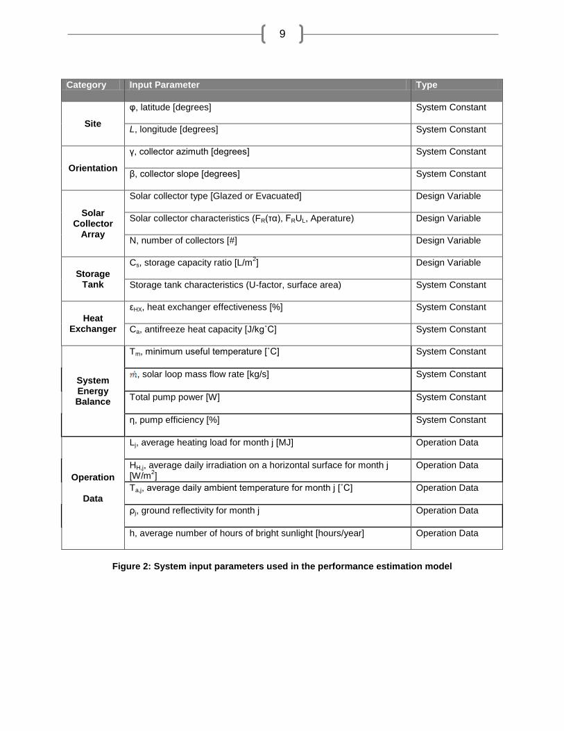
parameters used to define the system. The model parameters can be broken down into

three categories: design variables, system constants, and operation data. Design

variables are the main parameters that define the system. They are the variables that

are varied in the system analysis in order to find their optimum sizing. System constants

represent parameters that are either set at the beginning of the design or are

proportional to a design variable and so are not varied in the system analysis. Operation

data is required information necessary for calculations on the conditions under which

the system will be operating. Figure 2 lists the system parameters used in the

performance estimation model, and is followed by a brief description of each parameter.

9

Category Input Parameter Type

Site

φ, latitude [degrees] System Constant

L, longitude [degrees] System Constant

Orientation

γ, collector azimuth [degrees] System Constant

β, collector slope [degrees] System Constant

Solar Collector

Array

Solar collector type [Glazed or Evacuated] Design Variable

Solar collector characteristics (FR(τα), FRUL, Aperature) Design Variable

N, number of collectors [#] Design Variable

Storage Tank

Cs, storage capacity ratio [L/m2] Design Variable

Storage tank characteristics (U-factor, surface area) System Constant

Heat Exchanger

εHX, heat exchanger effectiveness [%] System Constant

Ca, antifreeze heat capacity [J/kg˚C] System Constant

System Energy Balance

Tm, minimum useful temperature [˚C] System Constant

, solar loop mass flow rate [kg/s] System Constant

Total pump power [W] System Constant

η, pump efficiency [%] System Constant

Operation

Data

Lj, average heating load for month j [MJ] Operation Data

HH,j, average daily irradiation on a horizontal surface for month j [W/m

2]

Operation Data

Ta,j, average daily ambient temperature for month j [˚C] Operation Data

ρj, ground reflectivity for month j Operation Data

h, average number of hours of bright sunlight [hours/year] Operation Data

Figure 2: System input parameters used in the performance estimation model

10

SITE

The longitude, φ, and latitude, L, of the site affect the relation of the sun to the site.

The official Toronto values given by Environment Canada were used (2).

ORIENTATION

The slope, β, is the angle that the plane of the collector makes with the ground. This

changes the angle of solar irradiation falling in the plane of the collector. Increasing the

slope increases the amount of irradiation on the collector during the winter and

decreases it during the summer. For maximum solar gain the rule of thumb is to set the

slope equal to the latitude ± 10 [degrees] (3 p. 157). In order to increase winter energy

generation when the demand is high at the expense of summer capacity when the

demand is low, a slope greater than the latitude was used. A slope of 50 degrees was

selected in order to simplify the mounting procedure.

Azimuth, L, is the angle between due south and the direction that the collector is

facing. The azimuth angle is set to zero for optimum solar energy gain (3 p. 158).

SOLAR COLLECTOR ARRAY

The solar collector array is the defining component of the SWH system. Its design

involves deciding upon the main design variables: collector type, collector product

model, and array size.

For this study two collector technologies were considered: Glazed Flat Panel and

Evacuated Tube. Suitable product models for each type of panel were identified based

on cost and performance. The performance estimation model was then used to

compare the performance of each of the collector types. This analysis resulted in the

11

selection of the Solarco SC-22 glazed flat panel as the collector product model. The

results of this analysis can be found in section 5.3.

The other key design variable in the solar collector array is the overall sizing of the

array. Using the performance estimation model, the number of panels needed to meet

the summer baseload was determined to be 55 panels for a total array area of 109.5

[m2].

STORAGE TANK

A thermal storage capacity ratio of 50 [L/m2] of collector area was considered for the

performance estimation. An insulated steel tank storage tank measuring 1.50 [m] in

diameter by 3.10 [m] in height with a U-factor of 0.3 [W/m2˚C] was selected.

HEAT EXCHANGER

An external shell and tube type heat exchanger with an effectiveness of 95% was

considered for the performance estimation.

The solar antifreeze fluid considered was a 50-50 propylene glycol / water mix with a

heat capacity of 5843 [J/kg˚C].

SYSTEM ENERGY BALANCE

The Φ,ƒ-Chart method requires the specification of a minimum temperature, Tm, that

must be surpassed for the solar fluid at the collector outlet to add energy to the system.

This minimum temperature was set as the expected return temperature of the service

hot water loop, which was estimated to be at 40 [˚C].

The mass flow rate of the solar loop, , was selected as the median of the range of

typical values described by Duffie and Beckman (4 p. 514). The mass flow rate used in

the performance estimation model was 1.64 [kg/s].

12

The total system pump power was roughly estimated by calculating the static head

and head loss experienced by the system. The total system pumping power was

estimated to be 2096 [W], assuming a pump efficiency of 85%. Details on this

calculation can be found in Appendix A.

OPERATION DATA

The time scale of the available radiation, temperature, and load data determines the

time scale of the estimation. Monthly average data was used in the performance

estimation, and is the most common time scale available. Since climatic conditions vary

greatly from year to year, it is beneficial to use data that has been normalized over a

number of years. Climatic data was provided by Environment Canada in the form of 30

year monthly average radiation and ambient temperature data (2). Load data was

provided by the TDSB in the form of 6 year monthly average normalized natural gas

consumption data for the boiler plant (5).

4.4. COST ESTIMATION

A comprehensive accounting of all the expected costs for the installation of the

system was performed in order to estimate the initial, annual, and periodic costs

associated with the project. This is presented in Figure 4.

Difficulty obtaining precise figures for worker wages, billable hours, and equipment

costs means that the cost estimation relies on assumptions made about these costs.

These assumptions present a degree of uncertainty into the cost estimation. In order to

estimate that degree of uncertainty, a range of values was used for each cost

13

assumption in order to generate a high and low cost estimate. These results are

presented below.

Estimate Selected High Low

Cost $86,434 $107,271 $68,426

Difference $20,837 -$18,007

± Percent 24% -21%

Figure 3: Pre-tax initial cost sensitivity

14

Figure 4: Initial, Annual, and Period cost estimation

Initial Costs Unit Quantity Unit Cost Amount Source

Design and Development

Permits project 1 318$ 318$ City of Toronto Permit Fee Schedule

Approvals p-h 5 70$ 350$ Estimate

Project management p-h 25 70$ 1,750$ Estimate

SWH system design p-h 18 70$ 1,225$ Estimate

Structural design p-h 6 70$ 420$ Estimate

Tenders and contracting p-h 10 70$ 700$ Estimate

Commissioning p-h 10 70$ 700$ Estimate

Construction supervision p-h 10 70$ 700$ Estimate

Sub-total : 6,163$

Equipment

Solar collectors # 55 750$ 41,250$ Quote from supplier

Collector support structure m² 109.5 135$ 14,776$ RETscreen user manual

Solar storage tank L 5500 2.13$ 11,688$ RETscreen user manual

Heat Exchanger kW 66 9.50$ 624$ RETscreen user manual

Piping materials m 48 25$ 1,200$ Cost survey

Auxiliary equipment project 1 300$ 300$ Cost survey/Estimate

Circulating pump(s) W 2,096 2.9$ 6,021$ Cost survey

Controls project 1 750$ 750$ Cost survey

Antifreeze L 78 7$ 543$ Quote from supplier

Sub-total : 77,151$

Installation

Roof mounting installation p-h 15 40$ 600$ Estimate

Solar Collector installation p-h 25 40$ 1,000$ Estimate

Plumbing installation p-h 20 40$ 800$ Estimate

Electrical installation p-h 15 40$ 600$ Estimate

Sub-total : 3,000$

Miscellaneous

Training p-h 4 30$ 120$ Estimate

Sub-total : 120$

Initial Costs - Sub-total : 86,434$

Initial Costs - Taxes : 12,101$

Initial Costs - Total 98,534$

Annual Costs Unit Quantity Unit Cost Amount Source

O&M

O&M labour p-h 2 30$ 60$ Estimate

Electricity kWh 5,613 0.10$ 561$ Estimate

Annual Costs - Total -$ 621$

Periodic Costs Period Unit Cost Amount Source

Replace Fittings 10 yr 300$ 300$ RETscreen user manual

Replace Antifreeze 10 yr 543$ 543$ Estimate

15

5. DESIGN RESULTS

5.1. OVERVIEW

Of all the system design considerations to take into account, the most important is to

select a design that is a suitable match for the building. In the system design phase,

suitable designs are identified and compared against each other on a qualitative basis.

The best designs are then passed on to the component design phase, where the

designs are compared on a quantitative basis.

5.2. SITE SELECTION

Using the site selection criteria, a suitable building was chosen for this feasibility

study. The facility is a 2 storey structure of masonry construction without a basement.

The original building was constructed in 1958 and has received major additions on

several occasions. The heated floor area measures 11,532 square metres, but the roof

area is 9,226 square metres, indicating that the approximately 80% of the floor area is

one storey. It is equipped with a cafeteria kitchen, full-size pool with showers, and is

host to various camp activities during the summer break.

The service hot water system for the school provides all the energy for space

heating, domestic hot water, and pool heating. It consists of 2 large winter boilers and

one smaller summer boiler. All of the boilers are reaching the end of their useful life and

will need to be replaced within the next 5 years, according to a site assessment

performed by the TDSB (6). As stated earlier, if the replacement equipment can be

downsized because of the installation of a SWH system, then savings may be assigned

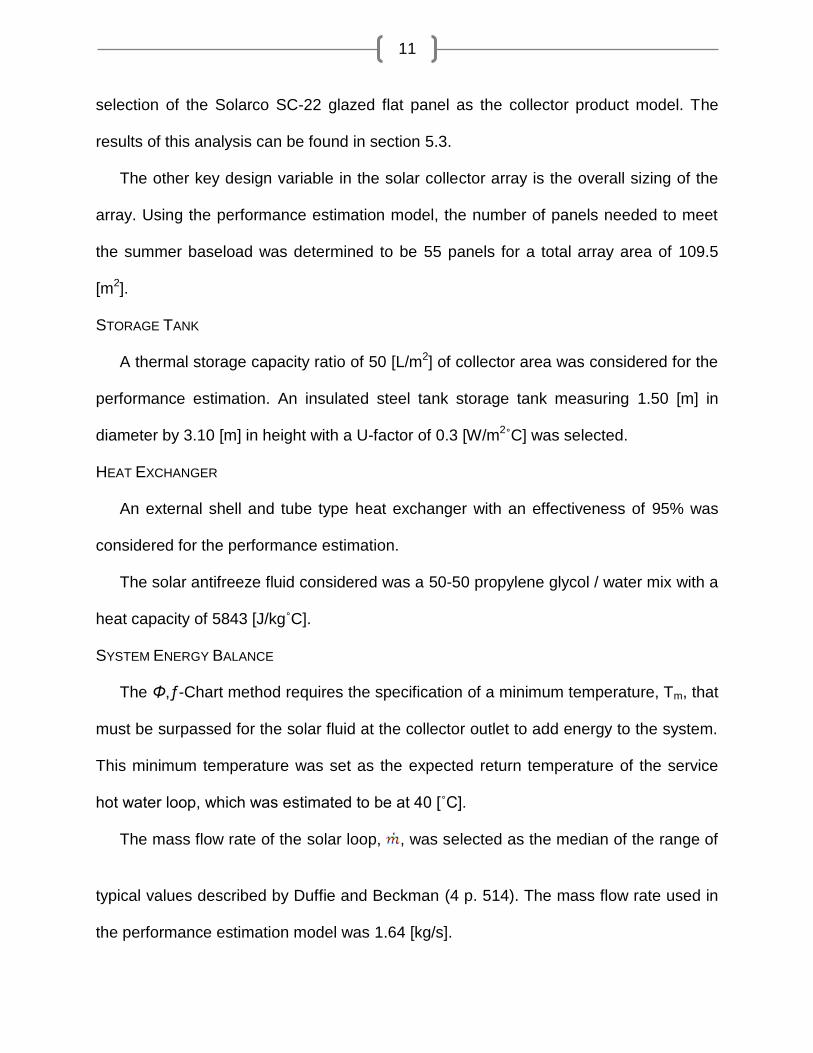
to the SWH system. A simplified diagram depicting the system is shown in Figure 5. For

16

these systems, the service hot water system operates on a closed loop. Heat is added

to the loop by the boiler plant and is removed by heat exchangers connected to the

loads. This system layout is very favourable to the addition of a solar water heating

system.

DHW Storage Tank

Boiler Plant

Pool

Radiators

and

Fan Coils

Natural Gas

To School From water

main

Figure 5: Simplified schematic diagram for the service hot water system

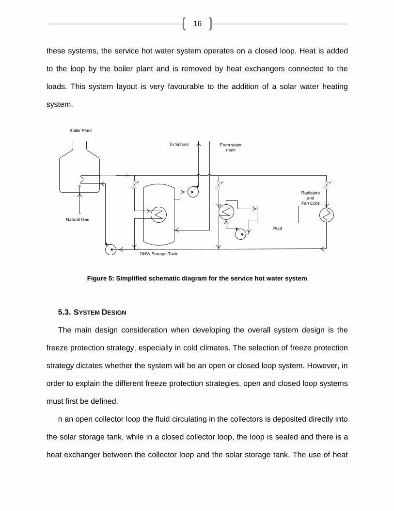
5.3. SYSTEM DESIGN

The main design consideration when developing the overall system design is the

freeze protection strategy, especially in cold climates. The selection of freeze protection

strategy dictates whether the system will be an open or closed loop system. However, in

order to explain the different freeze protection strategies, open and closed loop systems

must first be defined.

n an open collector loop the fluid circulating in the collectors is deposited directly into

the solar storage tank, while in a closed collector loop, the loop is sealed and there is a

heat exchanger between the collector loop and the solar storage tank. The use of heat

17

exchangers, which cannot perfectly convey all the heat from the hot water loop to the

load, reduces the amount of usable energy that can be drawn from the system. Figure 6

depicts the two system designs.

Figure 6: Closed and open collector loop designs

One of the main issues faced by solar water heating systems in an extreme

climate like Canada’s, is the possibility of freezing temperatures. If proper precautions

are not taken to ensure that water in the collectors or exposed piping does not freeze,

serious damage to the system can result. Two design strategies have been developed

to safeguard a system from possible freeze damage. The first design strategy is called a

draindown system, where electric or pressure actuated valves drain the fluid in the

collectors and exposed piping back into a storage tank while filling the collectors with

air. This design incorporates an open collector loop solar storage tank, and so is only

suitable in systems with this design. A concern with this freeze protection strategy is the

reliability of the of the draindown valve itself. Electrically actuated valves will not protect

the system in the event of a power failure, and pressure actuated valves are susceptible

to freezing shut in cold weather.

Hot Water Loop Supply

Solar Collector

Collector

Loop Pump

Hot Water Loop

Return

Hot Water

Loop

Storage

Hot Water Loop

Supply

Solar Collector

Collector

Loop Pump

Hot Water Loop

Return

Solar Collector

and Hot Water

Loop Storage

Closed Collector Loop Design Open Collector Loop Design

18

The second freeze protection design strategy uses a fluid with a very low freezing

point (antifreeze) as the collector fluid. This eliminates all risk of freeze damage in the

system, but due to the high cost of antifreeze, a closed collector loop with a heat

exchanger must be used. This again puts a constraint on the system design and

reduces the efficiency of the system, as described above.

The existing service hot water system in the school is a closed loop design which

serves the various loads through heat exchangers. This system is very easily modified

to incorporate a solar water heater loop in a boiler preheating configuration. This design

is beneficial because small temperature increases generated by the SWH loop can

reduce the fuel consumed by the boiler substantially. A closed collector loop design was

selected in order to facilitate the use of antifreeze as the collector fluid. The expense of

reduced performance and extra cost is justified, because in the Canadian climate robust

freeze protection is a must. This design was chosen because it offers the most reliable

and simple freeze protection. A diagram of the system design is shown in Figure 7.

Pool

Radiators

and

Fan Coils

Natural Gas

To School

From water

main

Boiler

Plant

DHW

Storage

Tank

HX

Solar Collector

Hot Water

Loop

Storage

Tank

HX

Figure 7: System design schematic

19

5.4. COMPONENT DESIGN

SOLAR COLLECTOR ARRAY

The solar collector array is the defining component of the SWH system. Its design is

the single most influential aspect of the system performance, both thermally and

economically. The design of the solar collector array involves deciding upon the main

design variables: collector type, collector model, and array size.

For this study two collector technologies were considered: Glazed Flat Panel and

Evacuated Tube. Suitable product models for each type of panel were identified based

on cost and performance. The selected panel models are manufactured by Solarco

Manufacturing Inc., a Toronto area company. Local sourcing reduces the expense

incurred when transporting the panels from their supplier. The performance estimation

model was used to compare the performance of each of the collector types. The results

of this analysis are given below.

Collector Type Model FR(τα) FRUL Aperature [m2/panel] Cost [$/panel]

Glazed SC-22 0.79 3.25 1.99 $ 750

Evacuated VCR-16 0.47 1.05 0.80 $ 900

Figure 8: Characteristics of selected solar collectors

Collector Number of Panels Total System Cost Energy Gain [MJ/year]

Tm = 40˚C Tm = 70˚C Tm = 100˚C

SC-22 (Glazed) 35 $ 59,235 141,661 84,545 38,906

VCR-16 (Evacuated) 87 $ 118,826 106,599 81,957 58,426

Figure 9: Results of comparison analysis, total array size = 70 [m2]

The results of this analysis provide an insight into the operation of the two collector

technologies. At lower minimum useful temperatures (Tm) the glazed collector is more

effective at collecting energy, while at higher temperature the evacuated collector is

more effective. This result agrees with the general collector efficiency graph shown in

20

Figure 1. Since the SWH system in this project is serving as a boiler preheater, high

temperatures are not required, so the benefits of the evacuated collector are lost. Also,

for the same area an evacuated collector array would cost nearly twice as much as a

glazed collector array, so the Solarco SC-22 glazed flat panel collector was selected for

use in this project.

The other key design variable in the solar collector array is the overall sizing of

the array. The number of panels and size of the array proportionally affect the amount of

energy generated by the system. The methodology for sizing the solar collector array is

to provide enough energy to just meet the summer baseload. Sizing the system for the

baseload demand is a good strategy to ensure that the system is never underutilized.

Also, a system which generates large amounts of unused energy during the summer

poses a danger to itself as it needs to vent the excess energy in a suitable fashion. If

pressure relief valves malfunction and the system heats up too quickly the pressure in

the solar loop can build up and cause a catastrophic failure, damaging the system and

endangering building occupants. Using the performance estimation model, the number

of panels needed to meet the summer baseload was determined to be 55 panels for a

total array area of 109.5 [m2].

THERMAL STORAGE

Thermal storage in SWH affects system performance in two ways. Firstly, it allows

solar energy to be saved for use at night or during periods of prolonged cloudiness.

Secondly, it increases the efficiency of the system by allowing the solar loop to dump its

energy even when the load is small. The storage tank was sized mainly considering

cost, constraining the selection within the acceptable range of storage capacity ratios

21

described by Duffie and Beckman (4 p. 540). A thermal storage capacity ratio of 50

[L/m2] of collector area was selected, yielding a total storage tank capacity of 5500 [L].

The size of an individual thermal storage tank is limited by the size of the door to the

boiler room. Fortunately, the boiler room of the selected school has a double door

opening to outside which could facilitate a maximum tank diameter of approximately 1 to

1.5 [m]. A storage tank measuring 1.50 [m] in diameter by 3.10 [m] in height was

selected. In terms of the storage tank construction, an insulated steel tank with a U-

factor of 0.3 [W/m2˚C] was selected. Steel tank construction was favoured over

fibreglass design due to the need for pressurization in the service hot water loop.

HEAT EXCHANGER

The closed collector loop design necessitates the use of a heat exchanger to

transfer heat from the solar antifreeze fluid to the service hot water fluid. In order to

achieve a high heat exchanger effectiveness, an external shell and tube type heat

exchanger has been selected. This requires pumps on both the solar fluid and service

fluid sides to circulate the fluids through the heat exchanger, which increases the

parasitic losses. The extra expense in equipment and operational costs is justified by

the increased ability to extract useful heat from the solar fluid. The external heat

exchanger configuration also facilitates easy maintenance and repair.

A 50-50 propylene glycol / water mix was selected for the solar antifreeze fluid due

to its low toxicity and effectiveness as a heat transfer fluid and antifreeze. The low

toxicity of propylene glycol is important in order to avoid the need for a double walled

heat exchanger. Double walls are often required as a safety measure in case of leaks,

helping ensure that the antifreeze does not mix with the potable water supply (6 p. 416).

22

It is to be expected that the existing domestic hot water heat exchanger is double

walled, since the service hot water loop likely contains bacterial inhibitor chemicals.

However, due to the age and condition of the existing equipment, it was decided to err

on the side of caution and select a non-toxic antifreeze fluid.

CONTROL SYSTEM

On/off operation of a fixed flow rate collector pump is the most widely used pump

and system control configuration (7 p. 101). Power switching controllers employ simple

electromechanical relays which are cheap, reliable, and familiar to installers. This

simple control scheme is possible because more complicated control points such as the

boiler control already have installed control mechanisms which react to the temperature

of the service hot water loop, irrespective of the SWH system.

The control system operates by measuring the difference between the collector

inlet temperature and the collector outlet temperature, ΔT. The system collects solar

energy by turning the pump on whenever ΔT reaches a preset amount, ΔTon. The

controller turns the pump off whenever ΔT drops to another preset amount, ΔToff. The

value of ΔToff is typically 0.5 – 1 ˚C and the value of ΔTon typically 4 – 6 times ΔToff (7 p.

102). Selection of these constants is important in order to reduce the frequency of

cycling that the will system experiences, which increases the parasitic losses incurred

by the pump.

23

5.5. PERFORMANCE RESULTS

The final system design was evaluated using the performance estimation model.

The resulting energy gains represent the performance of the system in a typical year.

The annual net solar energy delivered by the system was estimated to be 241,459 [MJ],

displacing 10,835 [m3] of natural gas. Parasitic pumping losses consumed 5,613 [kWh]

of electrical energy. Therefore the system generated 11.95 times more energy than it

consumed. The overall fraction of the total heating load supplied by the SWH system

was 2.69%, while the monthly solar fraction during July and August was 100%. Figure

10 charts the solar fraction as well as the total solar energy gain in [MJ].

Figure 10: Fraction of the heating load supplied by solar energy

Jan Feb Mar Apr May Jun Jul Aug Sep Oct Nov Dec

Energy Gain 9,024 14,300 22,017 25,719 28,919 29,430 28,658 27,615 28,863 20,680 5,775 2,853

Solar Fraction 0.0058 0.0105 0.0178 0.0370 0.0728 0.3296 1.0000 1.0000 0.1998 0.0379 0.0060 0.0019

0.0

0.1

0.2

0.3

0.4

0.5

0.6

0.7

0.8

0.9

1.0

0

5,000

10,000

15,000

20,000

25,000

30,000

35,000

Sola

r Fr

acti

on

Ene

rgy

Gai

n [

MJ]

24

6. FINANCIAL FEASIBILITY

6.1. EVALUATION METHODOLOGY

The economics of the project depend on several key financial factors: the availability

of a government subsidy, the energy cost escalation rate, the debt ratio and interest

rate, and the discount rate. The following section will describe the selection of those

factors as well as the economic indicators that will be used to evaluate the project.

GOVERNMENT SUBSIDY

Solar water heating installations are generally characterized by high initial costs and

low operating costs. Thus the basic economic problem is one of comparing an initial

known cost with estimated future operating costs. Reducing the initial cost can

substantially benefit the economics of a project, especially if debt is taken on for

financing. Many governments offer subsidies to renewable energy installation projects

to help offset costs and give the emerging technology a boost. The Government of

Ontario currently offers a rebate on the provincial sales tax for residential SWH

systems, however, a building such as the school considered in this project would not

qualify. Since 1998, the Canadian Federal Government has offered substantial rebates

through its Renewable Energy Deployment Initiative (REDI) program. The program

provides a refund of 25 percent of the purchase and installation costs of qualifying

renewable energy systems, to a maximum refund of $80,000 per installation (8). On

January 19th, 2007 Prime Minister Stephen Harper announced the cancellation of the

REDI program, and beginning of the the ecoENERGY program that will replace it. The

ecoENERGY for Renewable Heat program, will ―provide $36 million over four years to

increase the adoption of clean renewable thermal technologies for water heating and

25

space heating and cooling‖ (9). However, there has been no information made public

about the details of this program. For the purposes of this project, the assumption will

be made that the two programs are equivalent in their rebates. In order to gain insight

into the effect of government subsidies on the economics of SWH projects, the project

will be evaluated with and without this subsidy.

ENERGY COST INFLATION RATE

The energy cost inflation rate is that rate at which the price of energy is expected to

increase in the future. Selecting a suitable rate is difficult given the high degree of price

volatility that the energy market experiences. The methodology used in this analysis

was to use both the historic data and future projections. The historic 25 year overall rate

of increase in US natural gas prices was estimated at 43%, based on records from the

Energy Information Administration (EIA) (10). However, forecasts by the EIA predict that

natural gas prices will have declined by -0.7% by the year 2030 (11). Both figures have

discounted increases due to general inflation. Since it is likely that the true energy cost

inflation rate will fall within this range, the project will be evaluated at 0%, 20%, and 40%

overall 25 year energy cost inflation rates. This rate will be applied on top of a flat

general inflation rate of 2.0% based on current Canadian trends (12).

DEBT RATIO AND INTEREST RATE

The debt ratio is the percentage of the initial costs that were borrowed to finance the

project. This ratio changes the project economics because with increasing debt ratio

there will be increasing interest paid. The project will be evaluated at debt ratios of

100%, 50%, and 0% in order to examine its effect. The interest rate paid on debt was

26

selected at 6.0%, based roughly on the current (March 2007) prime rates for long term

closed loans (13).

DISCOUNT RATE

The discount rate represents an investor’s minimum acceptable rate of return on

investment, or in other words, the rate of return that would be earned had the money be

put into an alternate investment. The discount rate was selected at 4.0%, roughly based

on the current rate on long term government bonds in Canada (13).

ECONOMIC INDICATORS

Net Present Value (NPV) is defined as the present value of a series of cash flows,

evaluated at the discount rate. It is an indication of the profitability of an investment

minus the opportunity cost of an alternative investment returning at the discount rate (14

p. 152).

Simple Payback (SPB) is the amount of time it takes to recover the initial costs, not

taking into account the time value of money. It is simply the initial costs divided by the

income generated per year. It is a highly popular indicator due to its lack of dependence

on variables such as discount and interest rates, however, it is suggested not to rely

completely on this indicator since the timing of cash flows and duration of the project are

ignored (14 p. 155).

Discounted Payback (DPB), similar to simple payback, is the amount of time it takes

to recover the initial costs of a project. The discounted payback, however, takes into

consideration the time value of money. It is considered a more realistic indicator than

simple payback (4 p. 467).

27

6.2. ECONOMIC ANALYSIS

The economic analysis of the project was evaluated at differing values of three key

factors: the availability of a government subsidy, the energy cost escalation rate, and

the debt ratio. The project was evaluated over an expected lifetime of 25 years. The

results of these evaluations are given below.

Energy Cost Inflation Rate

No Subsidy With Subsidy

NPV SPB DPB NPV SPB DPB

0% -$44,573 25.22 Never -$14,768 18.92 Never

20% -$36,848 25.22 Never -$7,043 18.92 Never

40% -$28,127 25.22 Never $1,678 18.92 21

Figure 11: Case 1 – standard initial cost, 100% debt ratio

Energy Cost Inflation Rate

No Subsidy With Subsidy

NPV SPB DPB NPV SPB DPB

0% -$33,741 25.22 Never -$6,644 18.92 21

20% -$26,016 25.22 Never $1,081 18.92 18

40% -$17,296 25.22 23 $9,801 18.92 16

Figure 12: Case 2 – standard initial cost, 50% debt ratio

Energy Cost Inflation Rate

No Subsidy With Subsidy

NPV SPB DPB NPV SPB DPB

0% -$22,909 25.22 21 $1,480 18.92 17

20% -$15,184 25.22 20 $9,205 18.92 16

40% -$6,464 25.22 18 $17,925 18.92 15

Figure 13: Case 3 – standard initial cost, 0% debt ratio

Energy Cost Inflation Rate

No Subsidy With Subsidy

NPV SPB DPB NPV SPB DPB

0% -$9,321 17.76 Never $20,494 11.46 N/A

20% -$1,596 17.76 23 $28,219 11.46 N/A

40% $7,124 17.76 18 $36,939 11.46 N/A

Figure 14: Undersize boiler replacement, $30,000 savings in year 0, 100% debt ratio

28

6.3. SENSITIVITY ANALYSIS

The range of initial costs given in Figure 3 was used to perform a sensitivity analysis

on the cost estimation. The best case scenario (low cost estimation, 0% debt ratio) and

the worst case scenario (high cost estimation, 100% debt ratio) are presented below.

Energy Cost Inflation Rate

No Subsidy With Subsidy

NPV SPB DPB NPV SPB DPB

0% -$1,806 19.77 17 $17,307 14.82 14

20% $5,919 19.77 16 $25,033 14.82 13

40% $14,640 19.77 15 $33,753 14.82 12

Figure 15: Best case scenario – low initial costs, 0% debt ratio

Energy Cost Inflation Rate

No Subsidy With Subsidy

NPV SPB DPB NPV SPB DPB

0% -$73,873 31.42 Never -$36,743 23.57 Never

20% -$66,148 31.42 Never -$29,018 23.57 Never

40% -$57,427 31.42 Never -$20,297 23.57 Never

Figure 16: Worst case scenario – high initial costs, 100% debt ratio

6.4. DISCUSSION

The results of the economic analysis presented above gives an insight into the

economics of SWH systems. As was expected, financial feasibility increased with the

availability of a subsidy, increasing energy cost inflation rate, and decreasing debt ratio.

The most obvious trend in the economic analysis was the benefit of a government

subsidy towards the economics of the project. Under standard initial costing, no case

had a positive NPV without the aid of the subsidy. However, with the subsidy, all three

cases had the possibility of returning a positive NPV. The best case scenario (low initial

cost, 0% debt ratio) had a positive NPV without subsidy, indicating that if initial costs

could be lowered then financial feasibility without subsidy might be reached.

29

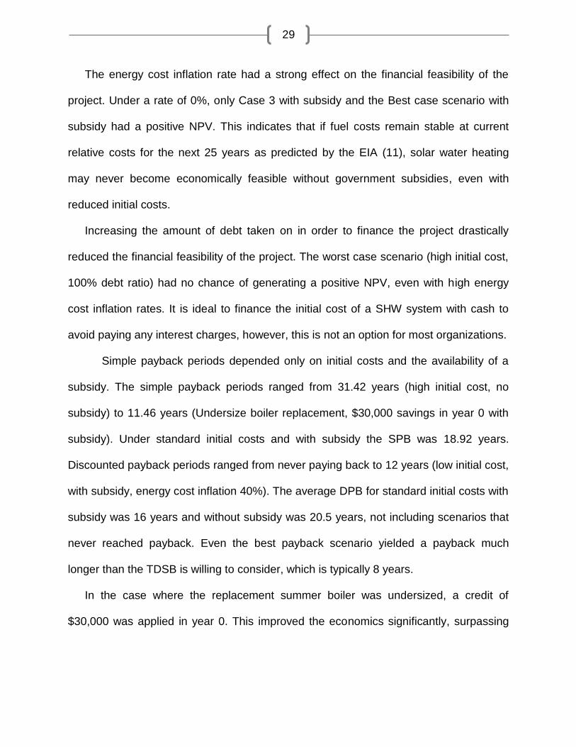
The energy cost inflation rate had a strong effect on the financial feasibility of the

project. Under a rate of 0%, only Case 3 with subsidy and the Best case scenario with

subsidy had a positive NPV. This indicates that if fuel costs remain stable at current

relative costs for the next 25 years as predicted by the EIA (11), solar water heating

may never become economically feasible without government subsidies, even with

reduced initial costs.

Increasing the amount of debt taken on in order to finance the project drastically

reduced the financial feasibility of the project. The worst case scenario (high initial cost,

100% debt ratio) had no chance of generating a positive NPV, even with high energy

cost inflation rates. It is ideal to finance the initial cost of a SHW system with cash to

avoid paying any interest charges, however, this is not an option for most organizations.

Simple payback periods depended only on initial costs and the availability of a

subsidy. The simple payback periods ranged from 31.42 years (high initial cost, no

subsidy) to 11.46 years (Undersize boiler replacement, $30,000 savings in year 0 with

subsidy). Under standard initial costs and with subsidy the SPB was 18.92 years.

Discounted payback periods ranged from never paying back to 12 years (low initial cost,

with subsidy, energy cost inflation 40%). The average DPB for standard initial costs with

subsidy was 16 years and without subsidy was 20.5 years, not including scenarios that

never reached payback. Even the best payback scenario yielded a payback much

longer than the TDSB is willing to consider, which is typically 8 years.

In the case where the replacement summer boiler was undersized, a credit of

$30,000 was applied in year 0. This improved the economics significantly, surpassing

30

even the best case scenario. However, a positive NPV was still only reached with the

availability of a government subsidy, or a high energy inflation rate.

31

7. CONCLUSION

The financial feasibility of a SWH project was found to be highly dependant on initial

costs, energy cost inflation rates, and debt ratios. This study found that under the right

conditions, such as utilizing an available subsidy, a high energy cost inflation rate, or a

low debt ratio, the installation of a SWH system could have a positive net present value,

indicating that the investment would a good one. However, many of the results of the

scenarios analyzed in this study found that under unfavourable conditions, such as the

opposite of those mentioned above, the system caused a net economic loss.

A specific case was examined where the addition of the SWH system allowed a

summer boiler to be undersized, resulting in savings for the SWH project and a boosted

financial feasibility. More research should be done into finding such niche applications

that maintain an acceptable level of comfort for the buildings occupants, but allow the

SWH system to fit into construction budgets.

The economic analysis indicated that if fuel costs remain stable at current relative

costs for the next 25 years as predicted by the EIA (11), large solar water heating

systems may never become economically feasible without government subsidies, even

with reduced initial costs.

Currently solar water heating systems seem to be poised right on the line between

profits and losses. It is up to the design team to create a system that is cost effective,

yet robust enough to provide free solar energy to its building for years to come.

32

8. REFERENCES

1. Andren, L. Solar Installations: Practical Applications for the Built Environment. London : The Cromwell Press, 2003. 2. A General Design Method for Closed-Loop Solar Energy Systems. Klein, S. A. and Beckman, W. A. 1979, Solar Energy, Vol. 22, pp. 269-282. 3. Environment Canada. Canadian Climate Normals 1971-2000 (Toronto, Ontario). National Climate Data and Information Archive. [Online] http://climate.weatheroffice.ec.gc.ca/. 4. Morehouse, J. Optimum System Design Techniques. [ed.] G. Lőf. Active Solar Systems. Cambridge : The MIT Press, 1993, pp. 152-180. 5. Duffie, J. A and Beckman, W. A. Solar Engineering of Thermal Processes. Hoboken : John Wiley & Sons, 2006. 6. Toronto District School Board. Internal Records. 7. Karaki, S. Space Heating: System Concepts and Design. [ed.] G. Lőf. Active Solar Systems. Cambridge : The MIT Press, 1993, pp. 411-463. 8. Bryon Winn, C. Controls in Active Solar Energy Systems. [ed.] G. Lőf. Active Solar Systems. Cambridge : The MIT Press, 1993, pp. 81-149. 9. Natural Resources Canada. Renewable Energy Deployment Initiative (REDI). Natural Resources Canada web site. [Online] Mar 2007. http://www2.nrcan.gc.ca/es/erb/erb/english/View.asp?x=692. 10. —. ecoENERGY Efficiency Initiative. Natural Resources Canada web site. [Online] http://www2.nrcan.gc.ca/es/erb/erb/english/View.asp?x=698. 11. Energy Information Administration. U.S. Natural Gas Prices. EIA web site. [Online] http://tonto.eia.doe.gov/dnav/ng/hist/n3020us3A.htm. 12. —. Forecasts and Analysis of Energy Data - Natural Gas Prices AEO. EIA web site. [Online] http://www.eia.doe.gov/oiaf/forecasting.html. 13. Statistics Canada. Latest Release from the Consumer Price Index. Statistics Canada web site. [Online] http://www.statcan.ca/english/Subjects/Cpi/cpi-en.htm. 14. Bank of Canada. Rates and Statistics. Bank of Canada web site. [Online] http://www.bankofcanada.ca/en/rates/index.html. 15. Szonyi, A. J., et al. Principles of Engineering Economic Analysis. Toronto : Wall & Emerson, Inc., 2003. 16. Klein, S. A. Design Methods for Active Solar Systems. [ed.] G. Lőf. Active Solar Systems. Cambridge : The MIT Press, 1993, pp. 39-76. 17. White, F. M. Fluid Mechanics. New York : McGraw-Hill, 2003. 18. City of Toronto. Building Permit Fee Schedule. City of Toronto web site. [Online] 2007. http://www.toronto.ca/building/fee_schedule.htm. 19. RETScreen International. RETScreen Software Online User Manual, Solar Water Heating Project Model. RETScreen International web site. [Online] 2005. www.retscreen.net.

33

9. APPENDIX A: PERFORMANCE ESTIMATION DETAILS

Φ,ƒ-CHART CALCULATION DETAILS

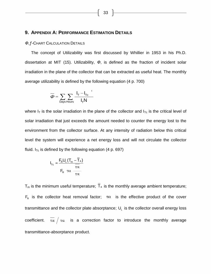
The concept of Utilizability was first discussed by Whillier in 1953 in his Ph.D.

dissertation at MIT (15). Utilizability, Φ, is defined as the fraction of incident solar

irradiation in the plane of the collector that can be extracted as useful heat. The monthly

average utilizability is defined by the following equation (4 p. 700)

T Tc

Days Hours T

I I

I N

where IT is the solar irradiation in the plane of the collector and ITc is the critical level of

solar irradiation that just exceeds the amount needed to counter the energy lost to the

environment from the collector surface. At any intensity of radiation below this critical

level the system will experience a net energy loss and will not circulate the collector

fluid. ITc is defined by the following equation (4 p. 697)

aR L mTc

R

F U (T T )I

F

Tm is the minimum useful temperature; aT is the monthly average ambient temperature;

RF is the collector heat removal factor; is the effective product of the cover

transmittance and the collector plate absorptance; LU is the collector overall energy loss

coefficient. is a correction factor to introduce the monthly average

transmittance-absorptance product.

34

As can be seen from the above equations, Utilizability is a function of climatic conditions

such as ambient temperature, collector fluid inlet temperature, and irradiation level, as

well as energy transfer characteristics of the chosen collector.

Due to the transient nature of these climatic conditions, however, the monthly

average utilizability, , cannot be approximated by substituting monthly average

climatic data into the equations above. Instead, it must be approximated through a

dimensionless correlation. cX Is the dimensionless critical radiation level, defined by (4

p. 700)

aR L mTc

c

T ot,n n R t,n n

F U T TIX

r R H F r R K H

The monthly average utilizability is calculated by the following correlation (4 p. 701)

2n

c cR

exp a b X cXR

2

T T

2

T T

2

T T

a 2.943 9.271K 4.031K

b 4.345 8.853K 3.602K

c 0.170 0.3061K 2.936K

The Φ,ƒ-Chart variables are then calculated as such (4 p. 704)

Tc RA F H NY

L

c R LA F U 100 tX'

L

The solar fraction can then be solved for numerically from (4 p. 707)

35

0.76

sY 0.015 exp 3.85 1 1 exp 0.15X' R

Where Rs is the ratio of the standard storage heat capacity per unit collector area of 350

[kJ/m2˚C]. ƒ is found for each month separately and multiplied by the monthly heating

load, L, to arrive at the monthly solar energy gain, Qu.

The following parameters need to be solved for previous to the above calculation.

δ , Solar Declination (4 p. 14)

284 n23.45sin 360

365

ωs , Sunset Hour Angle (4 p. 17)

s

sin sintan tan

cos cos

ωn , Solar noon Hour Angle (4 p. 17)

n 0

KT, Average Clearness Index: ratio of the monthly average radiation on a horizontal

surface to the extraterrestrial radiation (4 p. 72)

T

O

HK

H

rt,n, the ratio of hourly total to daily total radiation at noon (4 p. 82)

n st,n n

ss s

cos cosr a bcos

24sin cos

180

s

s

a 0.409 .5016sin 60

b .6609 .4767sin 60

36

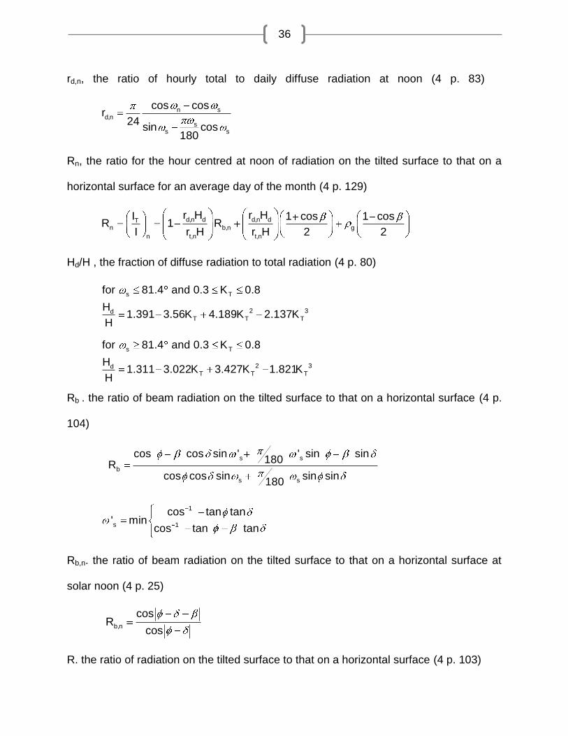
rd,n, the ratio of hourly total to daily diffuse radiation at noon (4 p. 83)

n sd,n

ss s

cos cosr

24sin cos

180

Rn, the ratio for the hour centred at noon of radiation on the tilted surface to that on a

horizontal surface for an average day of the month (4 p. 129)

d,n d d,n dTn b,n g

t,n t,nn

r H r HI 1 cos 1 cosR 1 R

I r H r H 2 2

Hd/H , the fraction of diffuse radiation to total radiation (4 p. 80)

s T

2 3dT T T

for 81.4 and 0.3 K 0.8

H1.391 3.56K 4.189K 2.137K

H

s T

2 3dT T T

for 81.4 and 0.3 K 0.8

H1.311 3.022K 3.427K 1.821K

H

Rb . the ratio of beam radiation on the tilted surface to that on a horizontal surface (4 p.

104)

s s

b

s s

cos cos sin ' ' sin sin180

Rcos cos sin sin sin

180

1

s 1

cos tan tan' min

cos tan tan

Rb,n. the ratio of beam radiation on the tilted surface to that on a horizontal surface at

solar noon (4 p. 25)

b,n

cosR

cos

R. the ratio of radiation on the tilted surface to that on a horizontal surface (4 p. 103)

37

d dTb g

H HH 1 cos 1 cosR 1 R

H H H 2 2

PUMPING POWER CALCULATION DETAILS

The first step is to calculate the pipe flow Reynolds number from (16 p. 353)

d

4QRe

d

If Red <= 2300 then the flow is laminar. Use the following equation to calculate the

friction factor (16 p. 353)

lam

d

64

Re

If Red >> 2300 then the flow is turbulent. Use the following equation to calculate the

friction factor (16 p. 366)

1.11

.5

tur d

1 6.91.8log

Re 3.7d

Now calculate the head loss using (16 p. 352)

2LVh

d2g

The required pumping power is then (16 p. 751)

s fgQ h hP

38

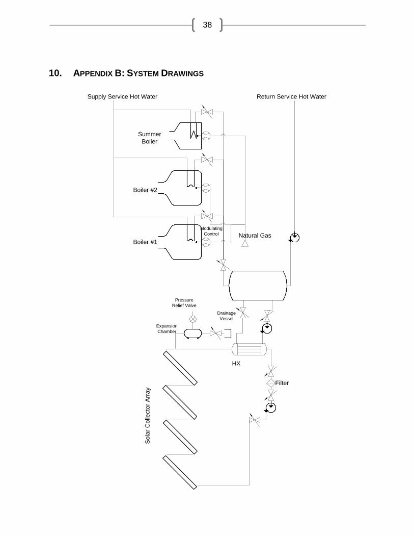
10. APPENDIX B: SYSTEM DRAWINGS

Boiler #1

Sola

r C

olle

cto

r A

rra

y

HX

Boiler #2

Summer

Boiler

Supply Service Hot Water

Expansion

Chamber

Natural Gas

Filter

Drainage

Vessel

Pressure

Relief Valve

Modulating

Control

Return Service Hot Water