thesis joe paton - white rose university...

ENERGY UTILISATION IN

COMMERCIAL BREAD BAKING

by

JOE BRAMWELL PATON

Submitted in accordance with the requirements for the degree of

Doctor of Philosophy

The University of Leeds

School of Mechanical Engineering

February 2013

Work Formed from Jointly Authored Publications

The candidate confirms that the work submitted is his own, except where work

which has formed part of jointly authored publications has been included. The

contribution of the candidate and the other authors to this work has been explicitly

indicated below. The candidate confirms that appropriate credit has been given

within the thesis where reference has been made to the work of others.

Chapter 5 is an extension of a conference paper that was presented at the 2012

EFFoST Annual Meeting (Paton et al., 2012a). The candidate conducted all the

experimental and computational analysis of bread provers that is presented in this

paper. The work was prepared under the guidance of all co-authors.

Chapter 6 is based on research that formed a journal paper published in Applied

Thermal Engineering (Paton et al., 2012b). A similar paper was also presented at

the Sustainable Thermal Energy Management International Conference 2011

(Paton et al., 2011). The system-level thermodynamic analysis methodology for a

commercial bread baking oven that is described in this paper was designed solely

by the candidate. The experiments conducted were also performed solely by the

candidate. The computational analysis presented in this paper was conducted by Dr

Khatir and forms no part of this thesis. The manuscript was prepared under the

guidance of all co-authors.

The oven temperature and velocity profiles presented in Chapter 6 have been

published in Applied Energy (Khatir et al., 2012c). This paper was previously

presented at the Sustainable Thermal Energy Management Conference 2010

(Khatir et al., 2010). The candidate conducted all the experiments and experimental

data processing for this paper. Dr Khatir conducted the computational simulations

which are not presented in this thesis. The manuscript was prepared under the


The experimental work in Chapter 7 has been used in Computational Fluid

Dynamics optimisation studies; published in Applied Energy in 2013 (Khatir et al.,

2013) and previously presented at the International Conference of Applied Energy

2012 (Khatir et al., 2012b). The candidate conducted all the experimental work

contained within these papers, including the graphs showing the optimum heat

transfer coefficient, which is also reproduced in Chapter 7 this thesis. Dr Khatir

completed the computational modelling work, none of which forms part of this

thesis. Furthermore, these same experimental results have been presented at the

2012 EFFoST Annual Meeting as part of a journal paper discussing oven

optimisation (Khatir et al., 2012a). These manuscripts were prepared under the


This copy has been supplied on the understanding that it is copyright material and

that no quotation from the thesis may be published without proper

acknowledgement.

© 2013 The University of Leeds and Joe Bramwell Paton

- ii -

Acknowledgements

Firstly, I would like to acknowledge my academic supervisors, Professor Nik

Kapur, Professor Harvey Thompson and Dr Malcolm Lawes. They have been a

constant source of encouragement and support and I wish to sincerely thank them

for their fantastic supervision and input. Special thanks also go to Dr Zinedine

Khatir, for his informal supervision. He has shared his experience and enthusiasm

with me throughout this project. I would also like to acknowledge Professor Vassili

Toropov for his input over the duration of this project. These colleagues have made

this PhD a joy and a privilege to complete.

It would not have been possible to complete this thesis without the help of a great

number of supportive industrial partners. From Warburtons: Colin Kelly, Trevor

Oakley and Sean Wincote assisted by giving the work a commercial perspective,

assisting with experimentation on commercial ovens and supplying historic data.

From Spooner Industries: Steve Newell, Dr Andrew Marson and Dan Kirk were

able to help me with contributing design details, advice on measurement techniques

and generous use of their excellent range of pilot oven facilities. Dr Patrick Horne

and Jacquie Quinton of SKM Enviros were helpful in extracting and manipulating

historic metering data from industrial bakeries.

My parents and family have been a tremendous source of love and support over the

years. Their interest in all things bread since I started this project has amused me,

as has their commitment to making sure their friends buy Warburtons bread over

the past three years. Thank you to each and every one of you.

There are a number of friends, whom I wish to thank for their assistance in

preparing this thesis – particularly their thoughts in discussing and proofreading

this work, including: Anthony McAndrew, Martin Quinn, Sam O’Sullivan, Richard

Mycroft, Gary Beahan and David Dollman.

Finally I would like to thank my partner, Lucy, whose love, patience and

motivation has helped me succeed. I especially thank her for putting up with me

over the last few years, through the hard times and the good.

- iii -

Abstract

The aim of this project was to benchmark energy utilisation of bread manufacturing

and to provide methodologies and results with the aim of improving efficiency in

commercial bakeries. The bread industry is an important provider of staple food

products across the world. Owing to the large energy use in bread manufacturing,

bakeries have come under increased scrutiny to reduce their environmental impact.

The proving process exposes dough to heat and humidity in order to encourage

yeast activation. Provers (responsible for 5 % of carbon emissions in bakeries) are

over-engineered to the extent that energy costs impact upon performance. The

industry standard practices that use large volumes of airflow to maintain food

safety have not been scientifically justified. Experimentally validated

Computational Fluid Dynamics (CFD) simulations showed the residence time

distribution profiles for different numbers of air changes. The results have indicated

that it is possible to reduce airflow by 33 % and electricity demand by over 70 %.

A system-level thermodynamic analysis was developed in order to measure and

model heat streams in industrial bread ovens. The model was subjected to a

sensitivity analysis to ensure the calculations could be trusted to give suitably

accurate results. A number of measurement techniques were employed and the

methodology was designed to increase the potential for industry-wide use to assess

the efficiency of ovens. The results showed that between 40 and 49 % of heat is

wasted in industrial ovens. The model has been successfully distributed to industry.

Experimental measurements of heat transfer for a range of regimes used in baking

ovens were undertaken. The results were validated by previous correlations

published in literature. Investigation focussed on three particular novel research

areas. Firstly, comparisons between nozzle types showed that rows of circular jets

could be approximated as slot nozzles for mean heat transfer. Secondly, the ratio of

convective to radiative heat transfer was investigated. Thirdly, the prevalence of

secondary peaks in local heat flux profiles was compared for two nozzle sets. These

unique results can be used to help design baking ovens with energy efficient

operating conditions.

- iv -

Table of Contents

Work Formed from Jointly Authored Publications .......................... 2

Acknowledgements ............................................................................... ii

Abstract ................................................................................................ iii

Table of Contents ................................................................................. iv

Figures .................................................................................................... x

Tables ................................................................................................ xvii

Nomenclature ................................................................................... xviii

Chapter 1 Introduction ..................................................................... 1

1.1 The Modern Bread Industry .................................................................... 1

1.2 The Global Energy Setting ....................................................................... 3

1.3 Principles of Bread Production ................................................................ 5

1.3.1 Formation of Dough ............................................................................ 6

1.3.2 Dough Proving ..................................................................................... 7

1.3.3 Bread Baking ....................................................................................... 8

1.3.4 Cooling .............................................................................................. 10

1.3.5 Slicing, Packaging and Distribution .................................................. 11

1.4 Research Aims and Objectives ............................................................... 12

1.5 Outline of Thesis ...................................................................................... 13

Chapter 2 Energy Use in the Baking Industry ............................. 14

2.1 Previous Studies ...................................................................................... 14

2.1.1 Bakery Energy Audits ........................................................................ 15

2.1.2 Life Cycle Assessments ..................................................................... 19

2.1.3 Baking Oven Energy Audits .............................................................. 21

2.1.4 Other Bakery Equipment ................................................................... 24

- v -

Chapter 3 Heat Transfer in the Bread Industry .......................... 27

3.1 Heat Transfer Fundamentals ................................................................. 27

3.1.1 Conduction ......................................................................................... 28

3.1.2 Convection ......................................................................................... 29

3.1.3 Thermal Radiation ............................................................................. 30

3.2 Jet Impingement Heat Transfer ............................................................ 32

3.2.1 Impingement Nozzles ........................................................................ 32

3.2.2 Air Jet Impingement in the Baking Industry ..................................... 34

3.3 Fluid Flow ................................................................................................ 37

3.4 Heat Flux Measurement ......................................................................... 38

3.4.1 Published Values for Convective Heat Transfer Coefficient ............ 39

3.5 Mass Transfer .......................................................................................... 41

3.5.1 Vaporisation and Evaporation ........................................................... 42

3.6 Thermal Imaging ..................................................................................... 42

Chapter 4 Computational Fluid Dynamics ................................... 45

4.1 Background .............................................................................................. 46

4.2 CFD in the Food Industry ...................................................................... 47

4.2.1 CFD in the Bread Industry ................................................................. 48

4.3 CFD Methodology ................................................................................... 52

4.4 Discretisation ........................................................................................... 53

4.4.1 The Finite Element Method ............................................................... 54

4.4.2 The Finite Difference Method ........................................................... 54

4.4.3 The Finite Volume Method ............................................................... 54

4.4.4 Mesh Generation ................................................................................ 55

4.5 Governing Flow Equations ..................................................................... 56

4.6 Boundary Conditions .............................................................................. 57

4.7 Turbulence Modelling ............................................................................. 59

- vi -

4.8 Validation and Verification .................................................................... 61

4.9 Summary .................................................................................................. 62

Chapter 5 An Experimental and Numerical Investigation of Industrial Bread Proving .................................................................... 64

5.1 Industrial Bread Provers ........................................................................ 65

5.2 Energy Use of Industrial Provers .......................................................... 67

5.2.1 Gas Consumption Trends .................................................................. 68

5.2.2 Air Handling Unit Electricity Consumption Trends .......................... 70

5.2.3 Steam Consumption ........................................................................... 72

5.2.4 Overall Energy Usage ........................................................................ 73

5.3 Problem Formulation ............................................................................. 74

5.4 Computational Fluid Dynamics (CFD) Model Design ......................... 75

5.4.1 Geometry ........................................................................................... 76

5.4.2 Turbulence Model Selection .............................................................. 77

5.4.3 Boundary Conditions ......................................................................... 77

5.4.4 CFD Solution Process ........................................................................ 79

5.5 Theory of Residence Time Distribution Analysis ................................. 79

5.6 Verification and Validation of Computational Model ......................... 82

5.6.1 Verification of Mesh Generation ....................................................... 82

5.6.2 Experimental Validation .................................................................... 83

5.7 Results ...................................................................................................... 84

5.7.1 Plots of Velocity Distribution ............................................................ 84

5.7.2 Numerical Results .............................................................................. 88

5.8 Residence Time Distribution Curves ..................................................... 89

5.9 Energy Savings ........................................................................................ 92

5.10 Summary .................................................................................................. 93

- vii -

Chapter 6 System-Level Thermodynamic Analysis of Commercial Bread Baking Ovens ..................................................... 95

6.1 Oven Configurations ............................................................................... 95

6.2 System-Level Energy Modelling ............................................................ 97

6.3 Theory of Energy Audits ........................................................................ 98

6.4 System-Level Model of a Commercial Baking Oven ......................... 100

6.4.1 Heat in via Gas Burner .................................................................... 102

6.4.2 Heat in via Steam Injection .............................................................. 102

6.4.3 Heat Required to Cook the Dough ................................................... 103

6.4.4 Heat Required for Moisture Evaporation ........................................ 104

6.4.5 Heat Uptake of the Tins and Lids .................................................... 104

6.4.6 Heat Uptake of the Oven Conveyor ................................................. 105

6.4.7 Heat in the Flue Gas ........................................................................ 105

6.4.8 Heat Loss from Oven Walls and Roof ............................................. 106

6.4.9 Total Heat Utilisation ...................................................................... 107

6.4.10 System-Level Thermodynamic Analysis Tool ................................ 107

6.5 Thermal Imaging ................................................................................... 109

6.6 Sensitivity Analysis of System-Level Model ....................................... 111

6.7 Sample Results ....................................................................................... 114

6.8 Opportunities for Energy Savings ....................................................... 115

6.8.1 Oven Insulation ................................................................................ 116

6.8.2 Conveyors ........................................................................................ 116

6.8.3 Tins and Lids ................................................................................... 116

6.8.4 Heat Recovery ................................................................................. 117

6.9 Temperature and Velocity Profiles in a Pilot Oven ........................... 118

6.9.1 Temperature Profiles ....................................................................... 118

6.9.2 Velocity Profiles .............................................................................. 121

- viii -

6.10 Summary ................................................................................................ 125

Chapter 7 Experimental Measurements of Local and Global Heat Transfer Characteristics ......................................................... 127

7.1 Background ............................................................................................ 127

7.2 Experimental Apparatus ...................................................................... 128

7.2.1 The Pilot Oven ................................................................................. 129

7.2.2 Nozzle Types ................................................................................... 131

7.2.3 The Heat Transfer Sensor ................................................................ 133

7.3 Methodology .......................................................................................... 135

7.4 Validation of Experiments .................................................................... 137

7.4.1 Repeatability .................................................................................... 137

7.4.2 Heat Flux Symmetry about Nozzle Centre ...................................... 139

7.4.3 Nusselt Number Correlations Compared with Literature ................ 140

7.5 Mean Heat Transfer Measurements ................................................... 143

7.5.1 Correlation of Nusselt Number with Reynolds Number ................. 143

7.5.2 Variation of Heat Transfer with Nozzle-to-Surface Distance ......... 144

7.5.3 Mean Proportion of Radiation and Convection ............................... 146

7.6 Local Heat Transfer Measurements .................................................... 148

7.6.1 Local Profiles of Nusselt Number with Reynolds Number ............. 148

7.6.2 Local Profiles of Nusselt Number with Dimensionless Nozzle-to-Surface Distance ........................................................................................... 150

7.7 Optimisation of Heat Transfer Coefficient for Energy Savings ....... 152

7.8 Summary ................................................................................................ 154

Chapter 8 Conclusions and Further Work ................................. 156

8.1 Conclusions and Main Contributions to Scientific Understanding .. 156

8.1.1 Computational Fluid Dynmanic Analysis of Bread Provers ........... 156

8.1.2 System-Level Modelling of Industrial Bread Baking Ovens .......... 157

- ix -

8.1.3 Experimental Measurements for Air Jet Impingement Heat Transfer for Regimes Relevant to Bread Baking ........................................................ 159

8.2 Future Work .......................................................................................... 160

8.2.1 Prover ............................................................................................... 160

8.2.2 Oven ................................................................................................. 162

8.2.3 Other Bakery Equipment ................................................................. 164

8.3 Summary ................................................................................................ 165

References .......................................................................................... 168

- x -

Figures

Figure 1.1 – Bar chart illustrating market segmentation of the worldwide and UK

bread industries (Datamonitor, 2011b, Datamonitor, 2011a) .................................... 3

Figure 1.2 – Graph of UK GHG emissions by source between 1990 and 2011

(Department of Energy and Climate Change, 2012) ................................................. 4

Figure 1.3 – Schematic diagram of the bread baking process ................................... 6

Figure 1.4 – Photograph of an industrial bread prover located above an industrial

oven (Warburtons Limited and Spooner Industries Ltd.) .......................................... 8

Figure 1.5 – Photographs of an industrial oven: (a) side view along oven length and

(b) view showing oven exit (Warburtons Limited and Spooner Industries Ltd.) ...... 9

Figure 1.6 – Photograph of the inside of a spiral bread cooler (Spooner Industries

Ltd.) ......................................................................................................................... 11

Figure 2.1 – Pie chart showing energy utilisation in a US bakery (Thumann and

Mehta, 2008) ............................................................................................................ 18

Figure 2.2 – Graph of heat distribution in commercial ovens from literature

(Johnson and Hoover, 1977, Whiteside, 1982) ........................................................ 22

Figure 3.1 – Graph of the thermal conductivity of bread as a function of

temperature (Monteau, 2008, Unklesbay et al., 1981, Wong et al., 2007) .............. 29

Figure 3.2 – Diagram of the flow field of an impingement jet ................................ 33

Figure 3.3 – Diagram of air impingement nozzles in a baking oven ....................... 35

Figure 3.4 – Dimensions of an ASME standard nozzle ........................................... 37

Figure 4.1 – Diagram of two-dimensional meshes: (a) structured and (b)

unstructured ............................................................................................................. 55

Figure 4.2 – Three-dimensional elements commonly used for mesh generation: (a)

hexahedra, (b) tetrahedra, (c) extruded triangles and (d) pyramids ......................... 56

- xi -

Figure 5.1 – Diagram showing the shape and dimensions of an L-type prover ...... 66

Figure 5.2 – Screenshot of online energy metering system for an industrial bakery

................................................................................................................................. 67

Figure 5.3 – Hourly gas use of a prover over the period of one week with mean

hourly gas use (4.1 m3) shown by red dashed line and the range of values within 1

standard deviation shown by blue dashed line ........................................................ 68

Figure 5.4 – Weekly gas use of an industrial prover over a period of one calendar

year with mean weekly gas use (633.4 m3) shown by red dashed line and the range

of values within 1 standard deviation shown by blue dashed line ........................... 69

Figure 5.5 – Hourly electricity use of a prover AHU over the period of one week

with mean hourly electricity use (23.4 kWh) shown by red dashed line and the

range of values within 1 standard deviation shown by blue dashed line ................. 71

Figure 5.6 – Weekly electricity use of a prover AHU over a period of one calendar

year with mean weekly electricity use (3,747 kWh) shown by red dashed line and

the range of values within 1 standard deviation shown by blue dashed line ........... 71

Figure 5.7 – Energy utilisation profile of an industrial bread prover ...................... 73

Figure 5.8 – CO2 emissions profile of an industrial bread prover ........................... 74

Figure 5.9 – Geometry for prover CFD model generated with assistance from

Spooner Industries Ltd. (Kirk, 2011) ....................................................................... 76

Figure 5.10 – Cross section diagram of prover showing the air ducting

arrangement, location of straps of tins and blue arrows illustrating the path of

airflow ...................................................................................................................... 77

Figure 5.11 – Partial view of prover CFD solution domain showing boundary

conditions and symmetry plane ............................................................................... 78

Figure 5.12 – Diagram of a mixing tank showing the concentration of the particles

injected at the inlet (A) at the outlet (B) with respect to time ................................. 80

- xii -

Figure 5.13 – C-diagrams as described by Danckwerts (1953) for: (a) piston flow

(b) piston flow with longitudinal mixing (c) complete mixing and (d) dead water. 81

Figure 5.14 – Velocity profile across a single prover vent, the second closest to the

loading/ unloading end, for five different mesh sizes/ numbers of elements .......... 82

Figure 5.15 – Pearson’s r correlation showing correlation with the finest mesh case

(1.39 million cells) for velocity profile across a single prover vent ........................ 83

Figure 5.16 – Validation of velocity profile along prover length with error bars

representing the experimental error relating to the apparatus used ......................... 84

Figure 5.17 – Isometric view contour plot of air velocity illustrating air distribution

throughout the prover volume ................................................................................. 85

Figure 5.18 – Angled top view contour plot of air velocity showing air distribution

down the prover length ............................................................................................ 86

Figure 5.19 – Velocity vector plot of air velocity showing flow paths of air through

a prover vent and around the product for the 13th plane parallel to a vent from the

loading end ............................................................................................................... 87

Figure 5.20 – End-on view contour plot of air velocity showing airflow distribution

around the tins for (a) the plane closest to the loading end, and (b) the 13th plane

from the loading end ................................................................................................ 88

Figure 5.21 – Prover section view from perpendicular to the xy-plane with red line

passing through the centre of the air vents offset in the z-direction by 5 mm ......... 89

Figure 5.22 – CFD predictions showing the air velocity profile along the prover

length for the red line shown in Figure 5.21 ............................................................ 89

Figure 5.23 – Residence time distribution for 2,469 particles ................................. 90

Figure 5.24 – Mean particle residence time as a function of the number of air

changes for both analytical and computational solutions ........................................ 91

Figure 5.25 – Percentage of particles not escaped the prover cavity after 360 s

residence time for each case .................................................................................... 92

- xiii -

Figure 6.1 – Schematics of two different oven designs: (a) direct-fired forced

convection and (b) indirect-fired radiant ................................................................. 96

Figure 6.2 – Diagram showing heat and mass flows within an industrial bread oven,

as detailed in Table 6.1 .......................................................................................... 101

Figure 6.3 – Input screenshot of oven thermodynamic energy analysis tool ........ 108

Figure 6.4 – Results screenshot of oven thermodynamic energy analysis tool ..... 108

Figure 6.5 – Thermal images of the roofs of two industrial bread baking ovens

showing the maximum (white text) and mean (green text) temperatures (°C) for

two ovens: (a) oven A and (b) oven B ................................................................... 110

Figure 6.6 – Thermal images of the outer walls of two industrial ovens: (a) oven A

and (b) oven B ....................................................................................................... 111

Figure 6.7 – Sensitivity analysis showing the effect on outputs based on a 10 %

change of each input variable ................................................................................ 112

Figure 6.8 – Compound sensitivity analysis based on changing each input variable

by the expected precision of the measurement and the instrument accuracy supplied

by the manufacturer ............................................................................................... 113

Figure 6.9 – Sample results of heat distributions obtained by system-level model

for two commercial baking ovens .......................................................................... 115

Figure 6.10 – Location of thermocouples across the oven width for a strap of five

tins .......................................................................................................................... 119

Figure 6.11 – Graph of temperature profile through a pilot oven for different

distances underneath the top nozzles: 20, 40, 60, 80 and 100 mm compared with

burner set point temperature (solid red line) .......................................................... 120

Figure 6.12 – Time averaged velocity profile of the top nozzles for three positions:

A – closest to the burner and C – furthest from the burner ................................... 122

Figure 6.13 – Time averaged velocity profile of the bottom nozzles for three

positions: D – closest to the burner and F – furthest from the burner ................... 123

- xiv -

Figure 6.14 – Three-dimensional profile of velocity through a pilot oven for top

nozzles: A – closest to the burner and C – furthest from the burner ..................... 124

Figure 6.15 – Three-dimensional profile of velocity through a pilot oven for bottom

nozzles: D – closest to the burner and F – furthest from the burner ...................... 124

Figure 7.1 – Partially labelled photograph of the pilot oven used for heat transfer

experiments ............................................................................................................ 129

Figure 7.2 – Schematic of the pilot oven used for heat transfer experiments ....... 130

Figure 7.3 – ASN arrangement for heat transfer experiments ............................... 132

Figure 7.4 – ARN arrangement for heat transfer experiments .............................. 132

Figure 7.5 – Photograph of Hukseflux RC01 heat flux sensor (Hukseflux Thermal

Sensors, c. 2010) .................................................................................................... 133

Figure 7.6 – Diagram of heat flux sensor (Hukseflux Thermal Sensors, c. 2010) 134

Figure 7.7 – Diagram showing minimum traverse range (P) of heat flux sensor .. 137

Figure 7.8 – Heat transfer graph indicating the degree of repeatability of the heat

flux profile measurements ..................................................................................... 138

Figure 7.9 – Dimensionless heat transfer coefficient of three nozzle profiles

overlaid on each other showing the degree of repeatability of the heat flux sensor

............................................................................................................................... 139

Figure 7.10 – Graph showing the degree of symmetry of heat flux measurements

about the nozzle centre .......................................................................................... 140

Figure 7.11 – Graph of Reynolds number against mean Nusselt number for ASN

experimental results and correlations reported in literature ................................... 141

Figure 7.12 – Graph of Reynolds number against mean Nusselt number for ARN

experimental results and correlations reported in literature ................................... 142

Figure 7.13 – Graph showing Nusselt number correlations for ASN and ARN ... 143

- xv -

Figure 7.14 – Regression plot to measure R2 value of data sets compared with

correlation .............................................................................................................. 144

Figure 7.15 – Martin (1977) correlations for dimensionless nozzle-to-surface

distance (H/d) against Nusselt number for ASN and ARN ................................... 145

Figure 7.16 – Comparison of experimental mean Nusselt number results for ARN

at varying H/d ratio with Martin (1977) ASN correlations ................................... 146

Figure 7.17 – Graph of Reynolds number against mean percentage of heat transfer

due to radiation for ASN ........................................................................................ 147

Figure 7.18 – Graph of Reynolds number against mean percentage of heat transfer

due to radiation for ARN ....................................................................................... 148

Figure 7.19 – Graph of local Nusselt number against dimensionless distance from

the centre of the nozzle jet (x/d) for ASN for five different Reynolds numbers

between 3,221 and 10,902 ..................................................................................... 149


the centre of the nozzle jet (x/d) for ARN for five different Reynolds numbers

between 3,771 and 11,801 ..................................................................................... 150


the centre of the nozzle jet (x/d) for two different nozzle types and H/d values ... 151


the centre of the nozzle jet (x/d) for different values of H/d for ARN .................. 151

Figure 7.23 – Predicted specific oven gas and electricity use as a function of heat

transfer coefficient ................................................................................................. 153

Figure 7.24 – Predicted bread baking carbon emissions equivalent per kg as a

function of heat transfer coefficient ....................................................................... 154

Figure 8.1 – Example of a Pareto front showing competing objectives: the objective

function, minimising cost (blue) and a critical quality objective (red) .................. 161

- xvi -

Figure 8.2 – Surface response of CFD optimisation study for optimising airflow in

and industrial bread oven (Khatir et al., 2013, Khatir et al., 2012d) ..................... 162

- xvii -

Tables

Table 3.1 – Emissivity values for materials relevant to bread manufacturing

equipment ................................................................................................................ 31

Table 3.2 – Emissivity values reported for bread from literature over a range of

temperatures (* temperature not given) ................................................................... 31

Table 5.1 – Equivalent carbon impact conversion factors for electricity and natural

gas (Carbon Trust, 2009) ......................................................................................... 73

Table 5.2 – Inlet boundary conditions for prover CFD model ................................ 78

Table 6.1 – List and explanation of energy flow streams for a typical commercial

baking oven (see Figure 6.2) ................................................................................. 101

Table 6.2 – Data statistics showing the variation of temperature in comparison with

burner set points for each oven zone ..................................................................... 121

Table 7.1 – Description of features of pilot oven .................................................. 131

Table 7.2 – Dimensions and specifications for the nozzle configurations

investigated ............................................................................................................ 133

Table 7.3 – Range of conditions for correlations between Reynolds number and

Nusselt number ...................................................................................................... 140

Table 7.4 – Changes to dimensions for correlating the asymmetric ARN as an ASN

............................................................................................................................... 142

- xviii -

Nomenclature

Abbreviations

AFR Air-fuel ratio

AHU Air handling unit

ARN Array of round nozzles

ASN Array of slot nozzles

BC Boundary condition

CAD Computer-aided design

CBP Chorleywood Bread Process

CFD Computational Fluid Dynamics

CIP Clean-in-place

EPSRC Engineering and Physical Sciences Research Council

FDM Finite Difference Method

FEM Finite Element Method

FVM Finite Volume Method

GHG Greenhouse gases

LCA Life Cycle Assessment

OEM Original equipment manufacturer

PID Proportional-integral-derivative

RANS Reynolds-Averaged Navier-Stokes

RCUK Research Councils UK

RHM Rank Hovis McDougall

RKE Realisable k-ε

RNG Re-normalisation group

SRN Single round nozzle

SSN Single slot nozzle

SST Shear-stress transport

TSB Technology Strategy Board

VSD Variable-speed drive

- xix -

Symbols

A Area m2

c Concentration mol/m3

cP Specific heat capacity J/(kg·K)

C Concentration of injected particles at outlet -

CV Calorific value J/m3

Cμ Variable used in the realisable k-ε turbulence model -

d Nozzle diameter (holes), nozzle width (slot) m

D Diffusion coefficient m2/s

E Energy J

Power W

Ea Activation energy J/kg

Esen Calibration factor of sensor V·m2/W

E(t) Exit age residence time function /s

f Relative nozzle area -

f0 Variable used in jet impingement correlations -

F Fraction of the fluid flow that is mixed at outlet -

g Acceleration due to gravity m/s2

h Heat transfer coefficient W/(m2·K)

h Height m

H Nozzle-to-surface distance m

Heat flow W

Hy Prover thickness in the y-direction m

J Diffusion flux mol/(m2·s)

k Turbulence kinetic energy m2/s2

K0 Pre-exponential factor /s

Kr Reaction rate -

L Length m

Le Latent heat of evaporation J/kg

Mass flow rate kg/s

- xx -

N Number of air changes per hour /hr

P Pitch between two sets of nozzles in the x-direction m

P Pressure Pa

q Heat flux W/m2

r Pearson Product-Moment Correlation -

R Universal gas constant J/(kg·K)

RH Relative humidity -

S Spacing between two round nozzles in the z-direction m

S Source term in the Navier-Stokes equations -

t Time s

Mean residence time s

T Temperature K

u Velocity vector m/s

u,v,w Velocity in the x, y and z-directions respectively m/s

V Volume m3

Volumetric flow rate m3/s

Vsen Voltage signal at sensor V

W Width m

x Distance from nozzle centre m

Greek symbols

α Degree of starch gelatinisation -

αk Thermal diffusivity as a function of temperature m2/s

β Volumetric thermal expansion coefficient /K

σ Stefan-Boltzmann constant W/(m2·K4)

σ Uniformity -

ε Rate of dissipation of turbulence kinetic energy m2/s3

εA Emissivity -

μ Dynamic viscosity W/(m2·K4)

ω Turbulence frequency -

- xxi -

λ Thermal conductivity W/(m·K)

ρ Density kg/m3

υ Kinematic viscosity m2/s

ϕ Interchangeable scalar variable for RANS equation -

ΓM Fluid viscosity Pa·s

ΓT Thermal conductivity in Navier-Stokes equation W/(m·K)

Subscripts

air Air

amb Ambient

atm Atmospheric

bread Bread

c Characteristic

cen Centre nozzle

crit Critical value

D Dynamic

e Evaporation

elec Electricity

gel Gelatinisation

in Inlet

l Lids

Mx, My, Mz Momentum equation in the x, y and z directions

noz Nozzle

P Constant pressure

s Surface of oven walls

sen Sensor

t Tins

T Total

w Water

wall Oven wall

- xxii -

x, y, z Position in the x, y and z direction

z1, z2, z3 Oven zones 1, 2 and 3

Dimensionless groups

Grashof number:

∆ for flat vertical plates

Δ

for horizontal flat plates

Nusselt number:

Prandtl number:

Rayleigh number:

∙

Reynolds number:

- 1 -

Chapter 1

Introduction

Bread is one of the oldest known and most important food products, having been

consumed worldwide for many millennia. The origins of bread can be traced back

as far as the Palaeolithic Period (c. 30,000 BC), as evidence of processing starch

has been has been found on ancient grindstones; it is thought bread was used as a

travelling food for wandering nomads and thus helped to populate the earth

(Revedin et al., 2010). It is believed that leavened (expanded dough produced by

yeast fermentation) bread was probably not consumed until Neolithic times (the

‘New Stone era’, c. 10,000 BC) when the chemical power of yeast was discovered

(Kent, 2012). By around 3,000 BC, bread became part an Ancient Egyptian’s staple

diet along with beer (Tannahill, 2002), and latterly became ubiquitous across the

world in Roman times. In modern times, it is one of few food products consumed

across both the developed and developing world and spans almost every culture.

Perhaps the most comprehensive description of the history of bread is given in the

book ‘Six Thousand Years of Bread, Its Holy and Unholy History’ that recalls the

social and political importance of bread over the years (Jacob et al., 1944). The

impact of bread upon society has been diverse; through religion: “Give us today

our daily bread”, politics – not least in early 19th century Britain where the

abolition of British corn laws made way for an international trade system (Kadish,

1996) – and in everyday colloquialisms: “The best thing since sliced bread”,

“Bread and butter”, “Bread-winner”, “Putting bread on the table”, “Dough”, etc.

1.1 The Modern Bread Industry

Commercial bread production occurs on a number of different scales, from artisan

bakeries serving the local community, to the large commercial bakeries serving

entire nations, as well as in-store/ supermarket bakeries, small chain outlets and

other sized bakeries in between. The focus of this thesis is large commercial

- 2 -

bakeries; i.e. bakeries producing bread at a rate of several tonnes of finished

product per hour on a continuous production process. The typical distribution range

of a commercial bakery of this magnitude can be up to hundreds of miles.

Although the core ingredients of bread are: flour, water, yeast, fat and salt, bread as

a product varies vastly depending on the ratio of these ingredients, additional

ingredients and production methods. The variations in taste and texture are

particularly noticeable across country borders. For example the British standard

loaf is largely unavailable in France, where the baguette is the mainstay product,

and in Germany (one of the highest consumers per capita); where darker, denser

products are often preferred. Further afield, Mediterranean bread is often

influenced by olive flavours, Middle-Eastern and Asian cultures typically consume

flat-bread type products whilst Latin-American countries consume more corn/

tortilla style baked products.

In 2010, the global bread and rolls industry was worth US $168.9 billion (£106.8

billion) per year and market value has been growing steadily by 2.2 to 2.4 % per

year since 2006. Annually, 93 million tonnes of bread are manufactured across the

world, of which 38 % is produced on an industrial scale, 48 % by artisan bakers, 9

% in-store and 5 % tortilla production (Datamonitor, 2011b).

The UK bread and rolls industry was worth US $4.9 billion (£3.1 billion) per year

in 2010 and market value has been growing marginally above average when

compared with global trends, at 2.4 to 2.6 % per year. Each year over 2.8 million

tonnes of baked goods are produced in the UK. Contrary to the global market

segmentation, a much higher proportion is produced in industrial bakeries (78 %),

with a smaller section of production in-store (16 %), with artisan production (4 %)

and tortilla production (2 %) making up the remainder (Datamonitor, 2011a). In

terms of the importance of the bread industry to economic prosperity, a 2010 report

stated that over 20,000 people are currently employed in UK bakeries (The

- 3 -

Federation of Bakers, 2010). Figure 1.1 shows graphically the difference between

the market segmentation of the UK and worldwide bread industries.

Figure 1.1 – Bar chart illustrating market segmentation of the worldwide and UK bread industries (Datamonitor, 2011b, Datamonitor, 2011a)

The baking industry has historically put little effort into monitoring or reducing

energy usage. However, with pressure mounting for industry as a whole to reduce

carbon emissions, use of fossil fuels and environmental impact, it is important that

commercial bakeries look to improve energy efficiency measures.

1.2 The Global Energy Setting

The global shortage of fossil fuels for energy generation and the harmful effects of

greenhouse gas (GHG) emissions on the environment are well documented. This

has forced policy-makers worldwide to devise strategies for reducing the

environmental impact of the human race. The distribution of GHG emissions across

all sectors in the UK is shown by Figure 1.2. Industrial processes have been

responsible for between 2.9 and 4.8 % of emissions between 1990 and 2011. In this

same period, industry reduced emissions by 47 % from 16.3 to 8.7 MTCO2e, whilst

total UK emissions (excluding power generation) have decreased by 19.4 % from

343.5 to 276.7 MTCO2e.

0%

10%

20%

30%

40%

50%

60%

70%

80%

Industrial Artisan bakers In-store Tortilla

Per

cen

tage

of

mar

ket

val

ue

Worldwide

UK

- 4 -

Figure 1.2 – Graph of UK GHG emissions by source between 1990 and 2011 (Department of Energy and Climate Change, 2012)

The member nations of the European Union and a host of other countries

worldwide are committed to reducing carbon emissions over the next few decades

as part of the Kyoto Protocol. The Kyoto Protocol was agreed in 1997 and is an

important addition to the United Nations Framework Convention on Climate

Change (UNFCCC) of 1994. As of June 2012, the Kyoto Protocol has been signed

and ratified by 191 States worldwide – most notably excluding the United States of

America and China. The Kyoto Protocol committed Annex I nations (including the

UK) to reduce GHG emissions by 5.2 % before 2012, based on 1990 base levels.

Furthermore, the UK Climate Change Act (2008) legally binds the UK government

to reduce carbon emissions by 80 % by 2050 based on 1990 base levels. In order

for these targets to be met, schemes such as the Climate Change Levy and the EU

Emissions Trading Scheme put financial pressure on, or offer incentives to,

industrial manufacturing sites to reduce carbon emissions. In addition to legislation,

soaring energy prices and diminishing fossil fuel reserves are encouraging industry

to reduce the amount of energy they use in order to cut costs and become more

environmentally responsible in the medium to long-term future. For these reasons,

0

50

100

150

200

250

300

350

400

1990

1991

1992

1993

1994

1995

1996

1997

1998

1999

2000

2001

2002

2003

2004

2005

2006

2007

2008

2009

2010

2011

GH

G e

mis

sion

s w

eigh

ted

by

glob

al

war

min

g p

oten

tial

(M

TC

O2e

)

Year

Industrial process Agriculture ResidentialPublic Transport Business

- 5 -

bakeries are one area of industry that has recently focussed efforts on energy

management.

1.3 Principles of Bread Production

Bread production encompasses a number of fundamental biochemical, chemical

and physical processes, such as: evaporation of water, volume expansion,

gelatinization of starch, protein denaturation, crust formation, carbon dioxide

production, formation of a porous structure and browning reactions (Purlis and

Salvadori, 2009a). Bread production on a commercial scale is frequently a

continuous manufacturing process, with short shutdown periods occurring on a

weekly basis to allow equipment to be cleaned and maintained. Several

engineering/ manufacturing issues in a commercial bakery need to be tightly

controlled in order for it to be commercially successful. First and foremost, product

quality is non-negotiable – this includes food safety, consistency of produce, taste,

texture, appearance and shelf-life. Furthermore, other factors such as minimising

interruptions to the manufacturing process to avoid wastage and keeping the

production time at a minimum are important to keep financial costs low. Energy

use is an increasingly important concern for commercial bakeries.

Bread is produced in five key stages:

1. Formation of dough: mixing and binding of raw ingredients and

shaping the dough pieces.

2. Proving: supplying the dough with heat and humidity to encourage the

yeast to ferment and the dough to rise.

3. Baking: heating the dough at high temperature to evaporate moisture

and convert fragile dough to stable bread.

4. Cooling: lowering the temperature of the bread to ambient.

5. Slicing, packaging and distribution: the final preparations are made

before the bread is delivered to the customer.

- 6 -

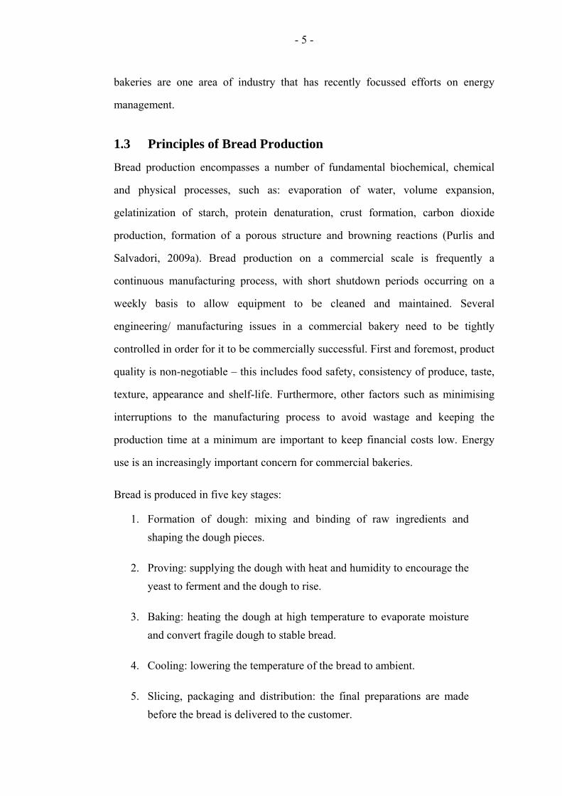
The manufacturing process, which typically takes around 4 hours, is shown

diagrammatically by Figure 1.3:

Figure 1.3 – Schematic diagram of the bread baking process

1.3.1 Formation of Dough

A typical bread recipe consists of flour, water, yeast, fat and salt. Mixing forms

these raw ingredients together into a dough-piece through the following processes:

Moistening: the surface of the bread is coated in liquid (often brine) to

prevent blistering.

Solubilisation: gluten proteins within the bread are dissolved into the dough

structure.

Swelling: the starch structure created by the gluten proteins begins to absorb

moisture and increase in volume.

Gluten formation: links between the proteins are formed which helps to

dictate the crumb structure of the loaf.

At this point the yeast begins to ferment which causes carbon dioxide gas cells to

form and creates an aroma (Stear, 1990).

All the major UK bread producers use the Chorleywood Bread Process (CBP) (or

the Chorleywood Method), which is a dough preparation technique developed in

Dough formation

Proving

Baking

Cooling

Slicing, packaging and

distribution

- 7 -

1961 by British Baking Industries Research Association (Beech, 1980). The

principle of the CBP is to ensure a set amount of mechanical energy is put into each

batch of dough in the mixing process at a much higher rate than historically used

(Cauvain and Young, 2006); typically this is 44.6 kJ/kg (Stear, 1990). Mechanical

energy is forced into the dough using large spiral mixers which allows the chemical

binding processes to initiate faster, subsequently causing the dough temperature to

increase. This temperature rise is not necessarily desirable in terms of nutrition;

therefore some critics favour traditional techniques which allow the dough to

develop more naturally with a much reduced energy requirement. Traditional

techniques are particularly favourable in terms of reduced salt content (Blanchard,

1965), which has led in part to the recent popularisation of artisan bread-making

(Owen, 2012). Two alternatives to the CBP are bulk fermentation and continuous

liquid fermentation (Fellows, 2009).

Once mixed, the dough is formed into individual pieces which will eventually form

the baked loaf. Depending on the product, the dough is either shaped using ‘4-

piece’ or ‘2-piece’ machining which affects product aesthetics, predominantly the

position and alignment of the gas cells within the structure and therefore the

direction of the crumb pattern – either across the width or height of a slice of bread.

1.3.2 Dough Proving

The proving (occasionally referred to as ‘proofing’) process prepares the dough for

baking by subjecting it to an elevated temperature and a high level of humidity in a

controlled environment. This process can take between as little as half an hour and

as much as half a day. During proving, yeast in the dough fermentation produces

carbon dioxide gas, thus expanding the size of the dough to roughly twice its

original size (Stear, 1990). The dough temperature is typically raised from

approximately 30 to 40 °C. Enzyme activity within the dough rapidly increases

once the temperature reaches 35 °C, therefore it is beneficial to increase the dough

temperature relatively rapidly to maximise the initial impact of the proving process.

- 8 -

Industrial provers can be up to 40 m in length. Provers in commercial bakeries are

often located in the space above a bread oven in order to use bakery space

efficiently and to indirectly recover heat from the oven roof, as indicated by Figure

1.4. Pre-heating technology has been trialled to raise the dough temperature before

the bread enters the prover, and thus reduce the energy load of the prover, however

the success reported has been limited (Cauvain and Young, 1998).

After proving the dough is in a fragile state as the carbon dioxide gas produced is

retained within a skin that forms on the surface of the dough. Until this skin is set

to become a crust (in the baking oven), the dough requires careful handling as any

disturbance can cause the structure to collapse.

Figure 1.4 – Photograph of an industrial bread prover located above an industrial oven (Warburtons Limited and Spooner Industries Ltd.)

1.3.3 Bread Baking

Baking encompasses a range of complex processes of simultaneous heat, water and

water vapour transport within the product as dough is transformed into bread. In

addition to dry heat, steam can also be used at the start of the baking process in

order to increase glossiness on the bread surface (Altamirano-Fortoul et al., 2012).

The main portion of the bake cycle subjects the dough to high temperatures in order

to initially deactivate the yeast and form a skin on the product surface. It has been

Prover

Oven

- 9 -

suggested that the complexity of the process is due to the comparatively high

temperature gradient and fast bake time in comparison with other drying processes

(Marcotte and Grabowski, 2008). Due to this complexity, there is a careful balance

throughout all parts of the manufacturing cycle to ensure that each process occurs

in synchronisation in order to produce a consistent and satisfactory loaf of bread.

Commercial bread ovens are typically tunnel-type ovens that can be up to 30 to 40

m long. The oven is often split into three zones so the baker can alter the profile of

conditions within the chamber, such as bake time, air velocity, air temperature and

steam injection. The baking profiles are dependent on the type of product that the

bakery is producing. Anecdotal evidence and experimentation has allowed

experienced oven operators to set baking conditions depending on factors such as

the ingredients, flavour/ texture required and expected weight loss. Photographs of

a commercial oven are shown by Figure 1.5:

(a)

(b)

Figure 1.5 – Photographs of an industrial oven: (a) side view along oven length and (b) view showing oven exit (Warburtons Limited and Spooner Industries Ltd.)

- 10 -

The main purpose of baking is to remove moisture from the dough, thus drying the

surface and forming a crust, resulting in significant mass transfer in the oven

(Klemes et al., 2008). Legislation for weight constraints for bread are tight

(typically ± 50 g for an 800 g loaf (Cauvain and Young, 1998)), so control of

moisture loss in the oven is critical. Excessive moisture loss from the product is

undesirable as this requires an increase in the quantity of raw materials at the start

of the manufacturing process and results in a higher energy demand to evaporate

the water content in the oven. In addition, decreased moisture loss often results in a

softer crumb and increased shelf life – two highly valued product characteristics

(Ovadia and Walker, 1998).

Once the dough temperature reaches 74 °C the gluten structure is set, therefore

carbon dioxide gas cells are retained in place within the bread, ensuring a porous

product (Fellows, 2009). Most academic researchers and industrialists agree that

bread is cooked once the core temperature reaches 96 to 98 °C (Ahrne et al., 2007,

Price, 2012, Purlis, 2011, Therdthai et al., 2002).

1.3.4 Cooling

The purpose of cooling is to lower the temperature of the bread in preparation for

slicing, packaging and distribution. As this is often the most time consuming

process in a bakery, coolers require a large quantity of physical space.

Bread is cooled in a humid environment (RH > 75 %) to minimise moisture

evaporation and the subsequent loss in mass. Due to this high level of humidity, it

is critical to monitor the air quality for bacteria to ensure food safety in line with

regulations. Product quality dictates that bread is usually cooled at atmospheric

temperature using no additional refrigeration or chilling load – this process can take

between 2 and 24 hours.

Coolers can be of a tunnel-type or a spiral conveyor; the inside of a spiral conveyor

cooler is shown by Figure 1.6. The bread travels on a conveyor in a helical motion,

- 11 -

often from bottom to top with the air flowing from top to bottom. This ensures a

more uniform temperature gradient between the bread and the air, thus increasing

the efficiency of the cooling process.

Figure 1.6 – Photograph of the inside of a spiral bread cooler (Spooner Industries Ltd.)

Typical conditions within a cooler are air temperature, Tair = 20 °C and air inlet

velocity, uin = 1 m/s (Cauvain and Young, 1998). More radical technologies, such

as vacuum cooling and active cooling (where the air temperature is chilled to below

ambient) exist in the food industry; however, due to the traditional nature of bread-

making bakeries have not widely adopted these to date.

Freezing of bread is possible, though it is well documented that this can have a

negative effect on the crumb structure, which can be negated by including additives

in the recipe (Ribotta et al., 2001). Food manufacturers are increasingly reluctant to

use additives as they are unpopular with consumers and can impact upon other

processes within the manufacturing cycle.

1.3.5 Slicing, Packaging and Distribution

The slicing, packaging and distribution phases of bread production make the bread

ready for consumption. Mechanical slicing machines ensure uniform width of

bread slices, depending on the product type, after which the loaf is placed into a

- 12 -

plastic bag or wax wrapped as appropriate and then it can be stored. Due to the

very short shelf-life of many baked products (typically less than 2 weeks),

production is very much governed on a supply-demand basis and very short stock

is held. Where stock is held it is often for smaller products (for example burger

rolls) and held in a freezer in anticipation of a production spike – which can occur

on a public holiday or during extreme weather. Distribution networks for

commercial bakeries can be vast (up to hundreds of miles), meaning delivery costs

are high. These costs can be variable due to fluctuations in oil prices, as the

majority of bread is delivered by road. Though this thesis does not address the

energy costs of product distribution logistics, it is an area of increasing concern for

bakeries for financial cost and environmental reasons.

1.4 Research Aims and Objectives

The aim of this study was to quantify the energy use in the proving and baking

processes of bread production and to investigate methods and technologies that

could be used to improve energy utilisation in the manufacture of bread on a

commercial scale.

The specific objectives of this research project were:

To understand the fundamental principles of heat and mass transfer, fluid

flow, industrial instrumentation and Computational Fluid Dynamics (CFD)

so that these analysis methods could be applied to investigate energy use in

the bread baking industry.

To analyse current prover energy consumption and to provide scientific

justification for quantifying the minimum number of air changes for a range

of provers, thereby directly reducing the energy demand and carbon

emissions of commercial bread proving.

To investigate the thermal energy efficiency of a variety of bread ovens and

generate a system-level thermodynamic analysis model that could be

- 13 -

applied to commercial bread ovens by use of non-invasive measurement

techniques to visualise opportunities for energy savings.

To conduct pilot-scale experimental heat transfer experiments to help

identify an optimum set of conditions for jet impingement heat transfer with

respect to energy usage that are practical for industrial bread baking ovens.

This work has been conducted through the use of both experimental and numerical

techniques to influence the engineering design and operational conditions of

industrial process equipment, with the overarching aim of reducing the energy

consumption and carbon emissions of the bread manufacturing process.

1.5 Outline of Thesis

This thesis addresses a number of key issues relating to energy use in bread baking.

The background of energy consumption in relation to bread manufacturing on

different scales is addressed in Chapter 2. Heat transfer as a general phenomenon is

discussed in Chapter 3, which also goes into detail on how this relates to bread

manufacture. Chapter 4 discusses the theoretical background of CFD and identifies

how best to utilise these tools in the analysis of process equipment. Chapter 5

presents an experimental and computational analysis of the energy consumption of

an industrial bread prover. A system-level thermodynamic analysis model for

baking ovens is described in Chapter 6. The methodology for, and results of, heat

flux experimentation for conditions relating to industrial baking are carried out in

Chapter 7. Finally, Chapter 8 discusses the implications of the work produced in

this project and concludes this thesis with some suggestions for further work.

- 14 -

Chapter 2

Energy Use in the Baking Industry

Bread production is considered to be an energy intensive process (Klemes et al.,

2008). There are a range of issues that have historically prevented the adoption of

energy efficient technologies in the baking industry, including: product quality,

hygiene fears, resistance to change, lack of capital investment and insufficient

resources to enable technologies to be trialled.

The current global political climate represents an opportunity for bakeries to make

step changes to lower the energy demand of baking bread. For instance, there are

funding opportunities in the UK through organisations such as: the Carbon Trust,

the Technology Strategy Board (TSB), the Engineering and Physical Sciences

Research Council (EPSRC) and the Research Councils UK (RCUK) Energy

Programme to both develop fundamental understanding and move innovations up

the ‘technology readiness levels’. Within the EU there are also grants that can

address these issues.

2.1 Previous Studies

A number of authors have addressed the issue of energy use in the baking industry.

These vary from detailed analyses of process equipment (Carvalho and Nogueira,

1997, Fuhrmann et al., 1984), to more general Life Cycle Assessments (LCAs) of

the environmental impact of producing and distributing baked goods (Andersson

and Ohlsson, 1999, Braschkat et al., 2003, Holderbeke et al., 2003).

The 1973 oil crisis in the US meant that energy use in process industries was a high

priority research area in the 1970s and early 1980s (Johnson and Hoover, 1977),

hence, a number of energy audits of bakeries were published between 1977 and

1984 (Beech, 1980, Casper, 1977, Christensen and Singh, 1984, Johnson and

Hoover, 1977, Laukkanen, 1984, Whiteside, 1982). After the resolution of the oil

- 15 -

crisis, energy supply had become less of a global concern and research into this

field appeared to decline. The recent intensification of research relating to energy

use in the process industries is due to environmental concerns and rising energy

costs. Bread ovens (and indeed other pieces of bakery equipment) have historically

been designed with little regard to energy use, with the main focus being on

product quality and production rates (Klemes et al., 2008).

There is a moderate amount of published research in the area of energy use in the

bread industry. Sections 2.1.1 to 2.1.4 summarise the findings of this published

literature and to critically analyse the contributions and disagreements between

authors in this field. As many of the most rigorous published methodologies and

datasets are over 20 years old, part of this thesis updates findings previously

reported for a modern industrial baking process. Although the principles of baking

have not changed significantly, the progressive changes in processing equipment

have had an impact on energy usage.

The following literature review categorises the previous research under the general

headings of: bakery energy audits, life cycle assessments, baking oven energy

audits and other equipment.

2.1.1 Bakery Energy Audits

Johnson and Hoover (1977) conducted an audit of a large industrial bakery in the

USA – this paper was published at the height of the oil crisis in the 1970s. The

authors gave mean energy use as 7.36 MJ/kg bread; which (in 1977) equated to 3.7

% of the product monetary value (US $0.0192/kg). As a proportion of the calorific

energy content of bread, four times the electricity and heat energy is required in

production. The recommendations presented in this report are generic, for example:

“unconventional ovens, such as steam and microwave, should be examined”, but no

specific improvements to process equipment were proposed. The suggestions for

further research of interest included: redesigning the shape of tunnel ovens,

- 16 -

recovering heat from flue gases and further analysis into the dough mixing

procedure.

Beech (1980) quantified energy use in three Rank Hovis McDougall (RHM) (Hovis

brand – now owned by Premier Foods) UK industrial bread plants, and compared

the primary energy use with that of home baking. It was reported the average

energy use in the bakeries was 6.99 MJ/kg, though the total energy use was 14.80

MJ/kg when the analysis included all processes from the growing of the wheat to

delivery to the consumer – i.e. the bakery processes accounted for 47.2 % of the

total energy used to produce a loaf of bread. Home baking with a gas oven used a

similar amount of energy, 7.84 MJ/kg, and with an electric oven 20.01 MJ/kg. The

figures for home baking depend largely on the method used – for example batch

size. This paper was critical of previous reports by Leach (1975) and Chapman

(1975), pointing out that there were very large differences in their results due to the

generalisations made by averaging out total energy use in the UK rather than

conducting a full on-plant energy audits.

Whiteside (1982) conducted energy audits of two bakeries in the USA. The specific

energy consumption of each was 1.89 and 4.16 MJ/kg and heat accounted for 80 to

82 % of the total energy. Although this report focussed mainly on the savings

possible by optimising process equipment within the bakery, opportunities for

energy savings were identified in the transportation of product. It is clear from

studying this report that the baking industry has become more automated since

1982 – for example the author makes reference to aligning processes according to

operator shift patterns, however due to use of automated machinery, shift patterns

no longer dictate production scheduling. The most pertinent energy saving

initiative outlined was to recover heat from the oven flue gas for use in the prover

via an air-to-air heat exchanger. The heating load of the prover and the amount of

heat rejected by the oven is similar and both pieces of equipment are at a fairly

constant heat load for the entire year. The idea is particularly feasible because of

- 17 -

the close proximity of the two units; therefore this solution is well suited for heat

recovery.

Laukkanen (1984) audited the energy use of 12 bakeries in Finland. The author

found that specific energy consumption varied between 3.2 and 11.5 MJ per kg of

bread produced (mean energy use was 6.5 MJ/kg). Energy costs in the bakeries

were between 1.5 and 3.7 % of turnover (in 1984). The mean production across all

bakeries was 1,220 tonnes per year for a range of production rates of between 88

and 7,740 tonnes per year. For each bakery, electricity accounted for approximately

a quarter of energy use, whilst the remaining fuel supply was light fuel oil. The

author agreed with other publications that ovens accounted for around half the

bakery energy use and further investigation on three different types of oven was

pursued. The other main energy uses were found to be for boilers and refrigerators.

It was reported that combustion in the ovens was inefficient because of air leaks to

the burners. The main suggestion for improvement was to recover heat from the

exhaust air; the danger of this is that the dust, flour and grease in the air could

cause damage to the heat exchanger equipment. Suggested use of the waste heat

included preheating supply air, using a heat pump to store the waste energy and

heating of service water or domestic hot water. The proposals outlined resulted in

potential 10 to 20 % reduction in energy consumption with payback periods of

between three and six years.

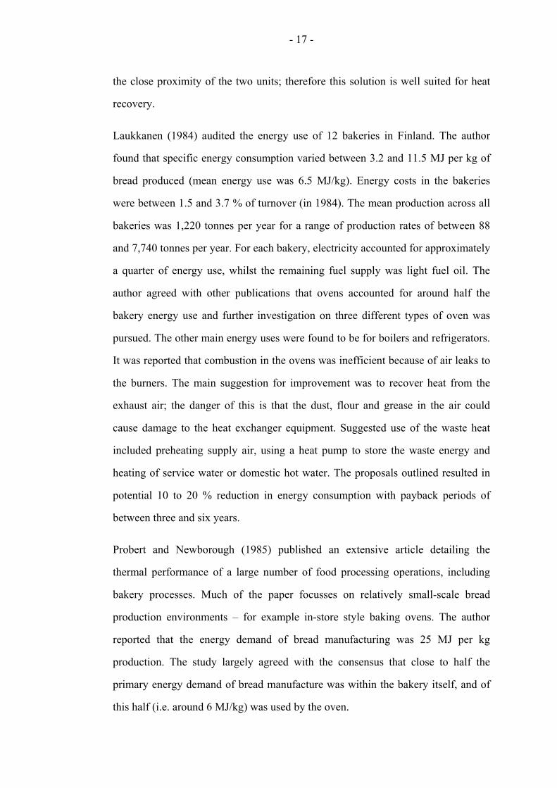
Probert and Newborough (1985) published an extensive article detailing the

thermal performance of a large number of food processing operations, including

bakery processes. Much of the paper focusses on relatively small-scale bread

production environments – for example in-store style baking ovens. The author

reported that the energy demand of bread manufacturing was 25 MJ per kg

production. The study largely agreed with the consensus that close to half the

primary energy demand of bread manufacture was within the bakery itself, and of

this half (i.e. around 6 MJ/kg) was used by the oven.

- 18 -

Kannan and Boie (2003) have outlined management practices for small sized

bakeries in Germany to reduce energy usage. Over 80 % of bakery produce is

manufactured in small local bakeries in Germany, in contrast with many

(particularly English-speaking) nations, where large industrial factories dominate

the bread industry – as illustrated by Figure 1.1. The baking process itself

accounted for 73 % of the total energy consumption, and 85 % was thermal energy.

Hot water generation to 70 °C was possible through heat recovery off the flue gas

from the oven, which improved efficiency by 10 to 15 %. It was also possible to

pre-heat burner combustion air which saved energy, reduced moisture content of

the air and reduced maintenance costs due to less tar build-up in the oil burners.

Energy reduction was expected to be 6.5 %, though doubt was raised as to whether

these cost savings were worthwhile as the capital cost was much greater than the

energy cost, given they are on a small-scale.

As part of a popular guide to energy auditing, an energy study on a US bakery was

produced (Thumann and Mehta, 2008). Having surveyed the literature, the numbers

presented in this book are in approximate agreement with the consensus, therefore

Figure 2.1 shows a graphical breakdown of the data:

Figure 2.1 – Pie chart showing energy utilisation in a US bakery (Thumann and Mehta, 2008)

21.5%

1.6%

1.4%

1.8%

10.6%

4.1%3.3%

3.0%1.8%1.8%1.1%

49.0%

Space heating

Air conditioning

Lighting

Domestic hot water

Pan washing

Mixers

Freezers

Cooking

Fryers

Proof boxes

Other bakery equipment

Baking ovens

- 19 -

Although a full detailed audit is not given, a breakdown of energy consumption

shows the primary energy user is the oven, consuming 49.0 % of the total bakery

use. Overall process energy totalled 73.7 % and domestic energy 26.3 %. Over a

fifth of the domestic energy use was “space heating” – though this is not a large

energy requirement in many bakeries located in milder climates.

The UK-based government organisation, the Carbon Trust, initiated a project in

2009 titled “Industrial Energy Efficiency Accelerator” (Carbon Trust, 2010). This

project focussed on giving UK bakeries a forum to collaborate on energy savings

ideas and to bring together research to improve process efficiency. This project

encompassed the three main commercial bakers in the UK: Warburtons, Allied

Bakeries (Kingsmill and Allinson brands), and Premier Foods (Hovis brand),

alongside smaller bakeries, equipment suppliers, academics and environmental

consultants. The initial report gave a solid overview of the UK baking industry. It

was reported that the total energy consumption was 2,000 GWh and emissions

were 570,000 TCO2/year. The breakdown of energy supply forms was: 560 GWh

electricity, 1,400 GWh natural gas and 40 GWh fuel oil. When the cost differential

between the three energy supply forms is taken into account, data for which is

supplied by the Department for Energy and Climate Change (DECC) (Carbon

Trust, 2012b) in the UK on a quarterly basis, this translates to energy cost of £38.2

million electricity, £44.7 million natural gas and £2.38 million fuel oil. These

numbers are is close agreement to the numbers discussed with technical

management of industrial bakeries (Oakley, 2009).

2.1.2 Life Cycle Assessments

Life Cycle Assessment (also known as: life cycle analysis, cradle-to-grave analysis,

integrated impact assessment or full cycle analysis) is a formal technique that

measures the environmental, health and resource impact of the material extraction,

production, use, recycle and disposal phases of a product (European Commission

Joint Research Centre: Institute for Environment and Sustainability, 2010). The aim

- 20 -

of a LCA is “to enable the incorporation of environmental and social impacts into

decision-making processes” (Sørensen, 2011). LCA principles, frameworks,

requirements and guidelines are governed by two international standards: ISO

14040 (International Organization for Standardization, 2006b) and ISO 14044

(International Organization for Standardization, 2006a). LCAs typically result in a

number of impact measurements, including: energy consumption, hazardous waste,

industrial waste, water waste, air emissions, noise, radiation and consumption of

raw materials (Rebitzer et al., 2004).

Andersson and Ohlsson (1999) aimed to establish the environmental effects of

producing bread on different scales in Sweden by use of LCA, by looking at home

baking, a local bakery and baking on an industrial scale. The impact of each has

been measured to include all processes from agricultural production, through to

flour milling, bakery processes, packaging and distribution. It was found that a

‘large’ industrial bakery (30,800 tonnes/year) had the highest carbon emissions and

used the most primary energy, 22 MJ/kg – though it should be noted that a large

industrial bakery in the UK may produce upwards of 200,000 tonnes/year. A

smaller industrial bakery, producing 12,800 tonnes/year, had similar performance

with relation to global warming, acidification and eutrophication as both home

baking and a local bakery – the primary energy usage was 14 MJ/kg. The reason

provided for the larger bakery using more specific energy was due to the large

distribution area – as the analysis included both delivery of raw materials to the

bakery and the delivery of the final product to the retail outlets and customers. In

terms of the baking processes, the economies of scale allowed the actual baking

process to be more efficient for the larger bakery. The authors suggested there was

a balance between the size of the bakery and distribution area which would give the

smallest possible environmental impact – the model for this would need to consider

factors such as population density, transportation method and positioning of

bakeries.

- 21 -

Three further LCA based papers were presented at the 4th International Conference

on “Life Cycle Assessment in the Agri-food sector” in 2003, and were published in

its proceedings (Braschkat et al., 2003, Holderbeke et al., 2003, Rosing and

Nielsen, 2003). Braschkat et al. (2003) reported that a ‘large’ bread factory used

around half the energy requirement of a bakery or home-production, however no

definition of ‘large’ was given. Rosing and Nielsen (2003) looked at the

environmental impact of different ways of making the holes in French bread for

hotdogs – concluding that any environmental concern was less important than

retaining the product brand and appearance. The study accounted for global

warming, acidification, eutrophication and nature occupation from storage of

ingredients to the storage of the finished product – thus, the processing and

transport of the ingredients, and the distribution of the finished product is not

included. Holderbeke et al. (2003), meanwhile reported that in the 19th century the

environmental impact of bread production was up to four times worse, due to

inefficient processes and the lack of quality fuels.

2.1.3 Baking Oven Energy Audits

As ovens have been shown to be the major energy users in bakeries, conducting an

energy audit would be the natural starting point for analysing energy utilisation in

the baking industry. Use of a rigorous scientific framework to measure energy

streams can help quantify the energy (both heat and electrical) that is useful to the

process and the energy wasted. Identifying waste energy streams and considering

ways to reduce waste is often a natural starting point for companies to audit

industrial equipment such as bread ovens.

Two historical energy audits presented here, from 1977 and 1982, give a good

baseline breakdown of heat distribution in industrial bread ovens. Although these

reports are not recent, this data is helpful to compare current technology and to give

an initial idea of thermal energy utilisation of commercial bread baking ovens.

Firstly, Johnson and Hoover (1977) reported that the baking process accounted for

- 22 -

28 % of the total energy usage of the entire manufacturing process. Of the oven

heat losses, 27 % was in flue gas and 10 % was through wall conduction. Only 15

% of the heat went into directly heating the bread whilst a large bulk, 40 %, of heat

was used to evaporate water from the dough. Whiteside (1982), however,

calculated that between 61 and 62 % of the energy use of the two ovens was

required for baking processes. Wall losses accounted for just 3 % whereas the

largest losses were stack losses (24 %). Figure 2.2 graphically compares these two

previous oven audits:

Figure 2.2 – Graph of heat distribution in commercial ovens from literature (Johnson and Hoover, 1977, Whiteside, 1982)

Christensen and Singh (1984) provided a review on advances in energy

technologies in the baking industry with reference to ovens manufactured by

Werner and Pfleiderer, Germany (now merged with Baker Perkins, UK) and more

generally, the Swedish baking industry. For this reason, there is the potential for the

report to have bias, particularly since it makes reference to an internal report by the

oven manufacturers. Despite this, there is a good explanation of methods used for

taking measurements and analysis. Mean specific energy use of the ovens was

0.898 MJ/kg for baking bread without lids, with lids this figure increased to 1.098

0

50

100

150

200

250

300

350

400

450

Heat to dough Moistureevaporation

StarchGelatinization

Flue losses Wall losses Heat to tinsand lids

Start up losses

Ove

n h

eat

flow

per

kg

bre

ad (

kJ/

kg)

Whiteside (1982) A

Whiteside (1982) B

Johnson & Hoover (1977)

- 23 -

MJ/kg. 44 % of heat input is lost through exhaust gas, ventilation and evaporation

of moisture from the dough. Only 19 % of the heat was transferred to the bread.

Heating of lids and pans was responsible for 17 % of the heat losses. Three main

suggestions were made to improve energy efficiency: (i) optimise the ventilation of

the ovens, (ii) review the materials used to manufacture pans and lids, and (iii)

recover heat from flue gases. No detailed explanation is given on how best to

approach realising these improvements.

Fuhrmann et al. (1984) reported on energy optimisation of heat streams by

recirculating hot air between different processes for a European-style baking

process. This research was also commissioned by Werner and Pfleiderer, indicating

potential for partiality. The innovation was centred on heat recovery; coupling the

high temperature exhaust of the prebaking oven with the lower temperature baking

oven. The authors suggested that heat recovery would make the bakery 3.7 % more

efficient. There are thorough explanations of methods used and how the

improvements were installed. The cost of making these improvements could only

be justified if energy costs were suitably high.

Carvalho and Nogueira (1997) analysed energy efficiency of furnaces, kilns and

baking ovens. There is a particular focus on free/ forced convection techniques and

variation in temperature profiles in these heating processes, thereby measuring heat

flux to the bread. Although the title of the paper implies that it is optimising energy

efficiency, the research focusses predominantly on global heat flux measurement in

baking ovens, a topic that is discussed in further in section 3.4.

Klemes et al. (2008) stated that baking is a large energy user in comparison to other

similar drying operations, such as preservation of fruit and vegetables. This is

because the thermal conductivity of bread is comparatively low and a large amount

of heat is needed to evaporate a significant fraction of moisture from the product.

The best measurement to gauge performance of baking ovens was reported to be

- 24 -

heat flux, which is dependent on the temperature gradient, air velocity and flow

characteristics. Heat flux can be measured with local sensors which are becoming

more commercially available and cost effective. Aside from offering opinions on

heat recovery, the authors also suggest that significant energy savings can be made

by optimising convective heat transfer within the ovens as this would reduce

baking time. Design of strategically placed nozzles allows the baker to remove

stagnant air from around the product and hence increase the rate of heat transfer.

Suggested improvements are low investment and it was suggested that they could

result in up to 20 % energy savings, however research is required to experimentally

(or otherwise) identify optimum conditions for heat transfer.

2.1.4 Other Bakery Equipment

Aside from general bakery audits and specific investigations on bread ovens, there

are other processes in bread manufacturing that have received little attention but

which offer the potential for energy savings.

Frank (2009) described recent attempts to reduce the energy consumption of the

baking industry in a commercial periodical “Baking Management”. In addition to

covering the widely-used industry techniques such as; boiler improvements, new

chillers, correctly sized and routed pumps/ pipes, lighting and other domestic

opportunities, interesting recent developments in the mixing process have been

outlined. An American machinery manufacturer appears to have invested heavily in

computational techniques to improve the mixing process by improving the cooling

effect and altering the shape of the mixing bowl. The results to show that use of a

variable-speed drive (VSD) to better control the mixing process can reduce energy

use and improve product quality. Heat recovery was also listed as an area for

further research, where a reduction of around 25 % of heat input can be realised.

There has been very little published research relating to energy use in the proving

process. Despite this, there is significant scope for reducing the energy use of

- 25 -

commercial bread provers, as shown by Paton et al. (2012a) and investigated in

Chapter 5. Much of the research into industrial bread proving is focussed on the

macroscopic changes to the dough structure as gas cells develop (Chiotellis and

Campbell, 2003b, Chiotellis and Campbell, 2003a, Cordoba, 2010, Grenier et al.,

2003, Grenier et al., 2010). Considering proving is responsible for upwards of 5 %

of the energy consumed in a bakery (Carbon Trust, 2010), the lack of scientific

research in this area is deterring bakeries from taking proactive measures to

optimise the process.

Cooling of food products can be an energy intensive process, particularly if the

temperature of a product needs to be reduced by a large amount, for example in the

freeze drying of foods such as ready meals (Pimentel and Pimentel, 2008). The

temperature gradient of cooling bread is comparatively large, and thermal

conductivity is typically low due to the porous nature of bread, which would

normally result in a high energy cost for cooling. However, the energy demand of

cooling bread is surprisingly low, since food quality/ safety dictates that there is no

requirement to cool bread quickly, nor is there a need to keep bread refrigerated or

frozen. For this reason, bread can be cooled over a longer period of time at ambient

temperature, resulting in a minimal energy demand. Despite this, in certain

circumstances, energy intensive cooling processes can be appealing to bakeries due

to the decreased cooling time and therefore potential to increase production rate

causing a reduction in the physical space the cooler occupies in a bakery. The two

most prominent alternative technologies to conventional methods are refrigerated

cooling and vacuum cooling.

Refrigerated cooling can be effective when the temperature difference between the

product and the ambient temperature is low (i.e. around 30 to 40 °C). Refrigeration

can significantly increase the temperature gradient and thus increase the cooling

rate. When the temperature difference between the product and ambient is large,

however, refrigeration does not increase the temperature gradient to a level where

- 26 -

the additional energy makes an impact to the cooling time. For this reason, two-

stage cooling has been recommended to initially reduce the temperature via

ambient cooling and finish the cooling process through refrigeration (James and

James, 2011).

Although vacuum cooling has been used since the 1950s in the horticultural

industry, much of the food industry has been reluctant to adopt vacuum coolers in a

production environment, mainly due to technological barriers (McDonald and Sun,

2000). The main benefits of vacuum cooling are: increased hygiene, improved food

safety, low weight loss, quicker cooling times, and the consequent potential

benefits of increased energy efficiency and a reduction in the size of machinery

required (Wang and Sun, 2001).

- 27 -

Chapter 3

Heat Transfer in the Bread Industry

As with most food production operations, transfer of heat in bread manufacturing is

of paramount importance to the success of the production process. Within the

bakery, the raw ingredients must be mixed together at ambient temperature,

exposed to humid conditions to encourage yeast fermentation, heated to

approximately 100 °C, and cooled again to ambient temperature within a confined

period of time, often in a continuous manufacturing environment. The major

characteristic of bread production, when compared to other heating processes, is

the porous nature of the product. Porosity is increased particularly during the

proving phase, when the bread expands and density decreases – this means that

thermal conductivity within the product is lower than many comparable heating

operations involving solids and liquids, meaning control of heat transfer becomes

critical. Many other physical changes in bread occur during the manufacturing

process that make measuring the heat demand a challenging task, for example

during proving the volume expands, during baking and cooling the moisture

content decreases and during mixing the dough rheology is constantly evolving.

3.1 Heat Transfer Fundamentals

There are several established textbooks that explain the main aspects of heat

transfer (Eckert, 1959, Incropera and DeWitt, 2007, Rohsenow et al., 1998, Russell

et al., 2008). The three fundamental forms of heat transfer are conduction,

convection and radiation – these are summarised in the following sections 3.1.1 to

3.1.3. Due to the complex nature of heat and mass interactions in real systems, heat

transfer is very rarely a result of just one of these three forms, although it is not

uncommon to have an overriding mode of heat transfer which deems the other

sources negligible. All three aforementioned modes have specific relevance to

bread production. For example in a baking oven, heat is transferred to the bread

- 28 -

through a combination of convection and radiation, and then heat is conducted

from the surface (crust) to the core of the crumb.

3.1.1 Conduction

Conduction is the transfer of heat from higher temperature to lower temperature

through the vibration of molecules. For most simple applications of conduction,

Fourier’s Law can be used. Fourier’s Law defines the rate of heat transfer as being

proportional to the temperature gradient across a material, dT/dx, shown in one-

dimension by Eq. (3.1):

(3.1)

where q is heat flux (W/m2), λ is thermal conductivity (W/(m·K)), A is surface area

(m2) and T is temperature (K).

Heat conduction is usually most effective in solids, in particular metals, due to the

molecular structure that allows a large number of electrons to vibrate and therefore

transfer heat. Thermal conductivity is a material specific property that is dependent

on factors such as temperature, phase and material structure.

Midden (1995), described the success of a baking operation as being dependent on

“the ability of the product to transfer heat from its outer surface to its center” i.e.

the rate at which conduction occurs from crust to crumb. As the temperature at the

core of the dough/ bread needs to be raised from ambient to approximately 100 °C,

conduction within the bread has a great effect on the energy requirement of both

the prover and oven.

Bread is a poor conductor of heat due to the cellular structure of gas cells trapped

within the dough/ bread. The thermal conductivity of dough/ bread varies with

temperature due physical changes in the material structure, i.e. volume expansion,

increase in porosity, decrease in density and moisture loss. Published temperature

dependent values of thermal conductivity for white sandwich bread vary between

- 29 -

0.11 and 0.85 W/(m·K) (Monteau, 2008, Unklesbay et al., 1981, Wong et al.,

2007). A summary of these studies is shown graphically by Figure 3.1. As with

other information presented in literature relating to the bread industry, the

variability across different studies means that the reliability of using any of the

reported data is compromised, therefore, for this study thermal conductivity values

taken from literature have been corroborated with industry to check the reliability.

Figure 3.1 – Graph of the thermal conductivity of bread as a function of temperature (Monteau, 2008, Unklesbay et al., 1981, Wong et al., 2007)

3.1.2 Convection

Convective heat transfer occurs when the movement of fluids causes momentum,

energy and mass transfer (Bacon, 1989). Two types of convection are frequently

discussed: free (or natural) convection and forced convection. Free convection is

typically driven by buoyancy forces, for example when hot air molecules rise

above cooler air due to temperature and density variations in an enclosed volume.

Forced convection requires an external force to encourage the fluid flow, for

example a pump forcing fluid to flow through a pipe or duct. The rate of convective

heat transfer is given by Newton’s Law of Cooling, Eq. (3.2):

(3.2)

0.0

0.2

0.4

0.6

0.8

1.0

0 50 100 150 200 250

Th

erm

al c

ond

uct

ivit

y (W

/(m

·K))

Mean internal bread temperature (°C)

Monteau (2008)

Unklesbay et al. (1981)

Wong et al. (2007)

- 30 -

where the convective heat transfer coefficient, hc, is dependent on a number of

physical characteristics of the fluid and flow parameters, thus, it is a difficult value

to determine numerically or theoretically. Two methods are frequently used to

calculate values – for simple flow problems it may be obtained by solving

boundary layer equations, or for complex flow it can be correlated using

experimental results (Incropera and DeWitt, 2007).

Values of heat transfer coefficient for gases in free convection regimes are typically

between 0.5 and 500 W/(m2·K), and for forced convection between 10 and 700

W/(m2·K). Section 3.4.1 gives a full review of published values for hc for bread

baking applications. For applications that use high velocity fluid flow and fluid

temperatures less than 400 °C, convection is often the dominant mode of heat

transfer.

3.1.3 Thermal Radiation

Thermal radiation is often considered the most complex mode of heat transfer

(Turner, 1993) and occurs when high energy photons are emitted from a hot body

in the form of electromagnetic waves. Unlike convection and conduction, no

particles are involved in the transfer of heat. Every object that has a temperature

greater than absolute zero (T = 0 K = -273.15 °C) will emit thermal radiation. A

‘black body’ is described as an object that will absorb radiation from every

wavelength and angle. The Stefan-Boltzmann Law (Eq. (3.3)) describes the heat

flux of a black body as the energy being proportional to temperature to the power

of four and shows that hotter and object is the more thermal radiation is emitted:

(3.3)

where the Stefan-Boltzmann constant, σ, is equal to 5.670 x 10-8 W/(m2·K4).

However, in reality objects will only absorb some of the heat available – these are

termed ‘grey bodies’. In order to apply Eq. (3.3) to a grey body, the emissivity, εA,

must be factored in and Eq. (3.4) is used:

- 31 -

(3.4)

Earle (2004) used this theory to estimate the heat transfer to a loaf of bread using a

value for total radiation as shown by Eq. (3.5):

1

1 1 1 (3.5)

The results showed that the heat transfer from the oven walls to the surface of the

bread was between 67.4 and 68.0 W (Earle, 2004). Table 3.1 shows emissivity

values for some relevant metals at bread baking temperatures (200 to 232 °C):

Material Temperature, T (°C) Emissivity, εA Reference

Aluminium:

smooth polished 227 0.05 (Brewster, 1992)

smooth oxidised 227 0.12 (Brewster, 1992)

rough oxidised 227 0.3 (Brewster, 1992)

Gold:

highly polished 200 0.03 (Aksyutov, 1974)

Stainless steel:

type 316 polished 232 0.57 (Cverna, 2002)

type 321 polished 149 to 815 0.18 to 0.49 (Cverna, 2002)

Table 3.1 – Emissivity values for materials relevant to bread manufacturing equipment

Values reported in literature generally agree on emissivity values for bread of

between 0.74 and 0.9, as shown by Table 3.2:

Temperature, T (°C) Emissivity, εA Reference

150 0.9 (Yanniotis, 2008)

* 0.9 (Hamdami et al., 2004)

* 0.9 (Purlis and Salvadori, 2009b)

177 0.85 (Earle, 2004)

* 0.9 (Sablani et al., 1998)

50 and 70 0.95 (Roberts et al., 2002)

80, 82 and 84 0.82, 0.79 and 0.76 (Gupta, 2001)

150 to 210 0.8 (Kress-Rogers and Brimelow, 2001)

Table 3.2 – Emissivity values reported for bread from literature over a range of temperatures (* temperature not given)

- 32 -

3.2 Jet Impingement Heat Transfer

Jet impingement heat transfer relies on fluid through an orifice (such as a nozzle) at

high velocity onto a surface. Fluid jet impingement is a technique widely used

across industry for drying, heating and cooling. Products manufactured using fluid

jet impingement include: plasterboard, foodstuffs, metal, paper, thin films, coatings

and packaging. High air velocity is used to increase heat and mass transfer rates,

often at the expense of increased capital and operating cost of equipment. Due to

this, impingement drying is only recommended for operations where a major

proportion of moisture is being removed (Mujumdar, 2007).

Jet impingement is an established technology in the food industry and has been

used in baking operations worldwide for several decades. The advantage of fluid jet

impingement is that the static boundary layer between the fluid and product is

reduced in size, which reduces the insulating effect between the hot bulk fluid and

cold surface and therefore allows higher rates of heat transfer. Moreira (2002)

noted that impingement nozzles ensured that convection is the dominant form of

heat transfer at the product surface.

3.2.1 Impingement Nozzles

Temperatures for applications of jet impingement have historically varied from -50

to 400 °C. Air jet impingement is characterised by sets of nozzles discharging air at

high velocity, typically between 10 and 50 m/s. It has been proved that for each

system there is a limiting velocity beyond which the boundary layer does not

decrease further, therefore heat transfer does not increase and using greater fluid

velocities would have no effect (Erdoğdu and Anderson, 2010).

The development of flow from a jet is of particular importance when designing an

impingement heating or cooling device. There are four characteristic regions of

flow of an impinging jet of air: the potential core, the free jet region, the

impingement region and the wall jet region – see Figure 3.2. There are two

- 33 -

important dimensionless ratios to consider when designing impingement nozzles:

dimensionless nozzle-to-surface distance, H/d, and dimensionless distance between

the nozzles, P/d and S/d (P is the pitch between two nozzle sets in the x-direction,

as shown in Figure 3.3 and S is the spacing between two round nozzles in the z-

direction). In addition, other geometric factors such as the nozzle shape contribute

to the rate of heat transfer.

Figure 3.2 – Diagram of the flow field of an impingement jet

Jet impingement nozzles commonly use either arrays of round nozzles (ARN) or

arrays of slot nozzles (ASN), although some applications may use a single slot

nozzle (SSN) or a single round nozzle (SRN). Martin (1977) developed a universal

set of correlations for all the aforementioned types of impingement nozzle. The two

important correlations for this study – ASN and ARN, are given by Eq. (3.6) and

Eq. (3.8) respectively. These equations use dimensionless numbers to calculate heat

transfer from air velocity. Dimensionless heat transfer is displayed as Nusselt

number, Nu and dimensionless air velocity is displayed as Reynolds number, Re.

.

23

. 2⁄ /

⁄

(3.6)

where f is relative nozzle area the variable f0 is defined by Eq. (3.7):

d

H

Potential core

Free jet region

Impingement region

Wall jet region

- 34 -

1

60 4 2⁄ 2 (3.7)

The correlation shown in Eq. (3.6) is valid for the below set of conditions:

1,500 ≤ Re ≤ 40,000

0.008 ≤ f ≤ 2.5·f0

1 ≤ H/d ≤ 40

. ⁄ , ∙1 2.2

1 0.2 ⁄ 6⁄ (3.8)

where K(H/d, f) is a variable defined by Eq. (3.9):

⁄ , 1/

0.6/

.

(3.9)

The above correlation is valid for the below set of conditions:

2,000 ≤ Re ≤ 100,000

0.004 ≤ f ≤ 0.04

2 ≤ H/d ≤ 12

3.2.2 Air Jet Impingement in the Baking Industry

In baking, air jet impingement is generally directed from both the top and the

bottom of the oven chamber onto the surface of the bread or tin, see Figure 3.3.

Ovadia and Walker (1998) described impingement technology as having

“revolutionised certain sectors of the baking industry”. At the time of the study it

was estimated that some 100,000 impingement ovens were in use. Two types of

impingement nozzles were described; short nozzles (orifices) and long thin nozzles

(jet tubes). The advantage of jet tubes is that there is a greater pressure drop across

the tube which increases airflow uniformity across an array of nozzles. Short

nozzles take up less space so are commonly used in smaller plants, for example

restaurants or in-store bakeries. Due to a smaller pressure drop, a more complex

design is necessary to maintain uniform air distribution across a bank of nozzles.

Yeast activation within the dough causes dough-based products to expand with

- 35 -

time (along the length of the oven). Due to this, the top surface of the bread rises

and therefore the distance between the air jets and the top surface of the product, H,

decreases. In some cases this is taken into account and the nozzle-to-surface

distance down the length of the oven is gradually increased to maintain optimum

H/d.

Figure 3.3 – Diagram of air impingement nozzles in a baking oven

A study by Sarkar and Singh (2004) considers factors such as hygiene and product

quality when assessing the suitability of jet impingement heat transfer in the food

industry. The authors note that jet impingement can often result in hot and cold

spots on the food if not correctly designed. In order to avoid this, the H/d ratio must

be carefully considered – it must be large enough to give an even distribution of air

across the product and small enough to give optimum heat transfer rates for quality

and efficiency purposes.

The effect of jet impingement for both heating and cooling of food is investigated

by Olsson and Trägårdh (2007), where CFD and experimental results were

compared. The importance of ensuring that the interaction between multiple jets is

modelled and validated experimentally is emphasised – as this has a significant

d Direction of product

Nozzle orifices Airflow

Product

P

- 36 -

effect on the flow field and heat transfer to the product. The same authors presented

two further CFD studies on heat transfer from impinging air jets onto cylinders

(Olsson et al., 2004, Olsson et al., 2005). The cylinders have a diameter of 35 mm

and were given the properties of a generic food product to represent the baking

process. The jets investigated were slot jets with a width of 30 mm. The effect of a

single jet, two jets and three jets were investigated, by varying the Reynolds

number, distance between nozzles and exhaust opening area. It was found that there

was a slight increase in heat transfer with a H/d ratio of 2 compared with H/d = 8,

and there was a significant increase in heat transfer for higher Reynolds numbers –

the correlation derived for Nusselt number was in the form of Reynolds number to

the exponent 0.59. Larger exhaust openings resulted in significantly lower heat

transfer.

A number of authors describe the relation between nozzle parameters and heat

transfer in technical detail (Das et al., 1985, Gardon and Akfirat, 1966, Lytle and

Webb, 1994, Martin, 1977). Different spatial arrangements of jets, and distances

between them can create stagnation points which will negatively affect heat

transfer. The key parameters for ensuring efficiency of heat transfer are: fluid flow

rate, nozzle diameter, nozzle spacing and the nozzle-to-surface distance. The

relevance of this highly academic literature to industry is questioned by Marson

(1999), who states that much of the derived correlations are for a single slot nozzle

or a single round nozzle, whereas in reality industry uses arrays of nozzles for the

vast majority of drying applications.

In addition, ‘ASME Standard’ nozzles are almost always used for these

experiments, which use geometries that are specifically designed to give very high

discharge coefficients (close to unity) to generate flow streams close to

theoretically calculated conditions. However, in reality nozzles can rarely be

manufactured cost-effectively to this standard, in which case the flow

characteristics used in commercial dryers are significantly different to those

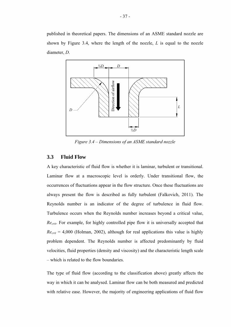
- 37 -

published in theoretical papers. The dimensions of an ASME standard nozzle are

shown by Figure 3.4, where the length of the nozzle, L is equal to the nozzle

diameter, D.

Figure 3.4 – Dimensions of an ASME standard nozzle

3.3 Fluid Flow

A key characteristic of fluid flow is whether it is laminar, turbulent or transitional.

Laminar flow at a macroscopic level is orderly. Under transitional flow, the

occurrences of fluctuations appear in the flow structure. Once these fluctuations are

always present the flow is described as fully turbulent (Falkovich, 2011). The

Reynolds number is an indicator of the degree of turbulence in fluid flow.

Turbulence occurs when the Reynolds number increases beyond a critical value,

Recrit. For example, for highly controlled pipe flow it is universally accepted that

Recrit = 4,000 (Holman, 2002), although for real applications this value is highly

problem dependent. The Reynolds number is affected predominantly by fluid

velocities, fluid properties (density and viscosity) and the characteristic length scale

– which is related to the flow boundaries.

The type of fluid flow (according to the classification above) greatly affects the

way in which it can be analysed. Laminar flow can be both measured and predicted

with relative ease. However, the majority of engineering applications of fluid flow

L

D ¾D

D

½D

Dir

ectio

n of

air

flow

- 38 -

result in some degree of transitional or turbulent flow, which can make measuring

of predicting the flow characteristics more challenging. Experimental measurement

of turbulent flow can result in unstable readings and whilst numerical predictions

can be accurate on an overall basis, they are often unable to convey the degree of

instability of the flow.

The Euler equations are used as governing equations for fluid motion. The

Bernoulli Equation is a common way to display the momentum part of the Euler

equations, and is suitable for analysis of non-viscous, incompressible flow. Derived

in the 18th Century by the Swiss scientist Daniel Bernoulli, Bernoulli’s Equation is

useful for analysing flow as a function of pressure difference. Eq. (3.10) gives

Bernoulli’s equation in one-dimensional format assuming no frictional losses and

for incompressible, smooth fluid flow.

12

12

(3.10)

where P is total pressure (Pa), u is fluid velocity (m/s) and h is height (m).

The Navier-Stokes Equations are again derived from the Euler Equations and

define mass, momentum and energy conservation of fluid flow, and are used

extensively in numerical modelling. Notably difficult to solve analytically, the

equations become useful when predicting local properties of fluid within a domain

and are discussed further in Chapter 4.

3.4 Heat Flux Measurement

Childs et al. (1999) discussed a number of techniques that can be used to determine

the heat transfer to an object in a seminal paper on heat flux measurement. The

methods vary in ease and intrusiveness to the process. The four methods discussed

were: differential temperature, calorimetric methods, energy supply/ removal and

mass transfer analogy. Differential temperature is the use of thermopiles to

accurately measure the conduction of heat across a material. Calorimetric methods

- 39 -

use time-averaged measurements of temperature to conduct a heat balance by

calculating the rate of change of thermal energy of a material. Energy supply or

removal is when a known quantity of heat is transferred to or from the sample

surface to create a thermal equilibrium to measure the heat flux. Finally, it is

possible to measure mass transfer and relate this to heat transfer using

mathematical relationships between the two related principles. The most suitable in

the scope of this project was the differential temperature method as heat flux

sensors using this theory are commercially available. This technique uses principles

of Fourier’s Law, “temperature differential across a spatial distance within a

medium”, which can infer heat flux by measuring the temperature gradient across a

material with a known thermal conductivity.

Carvalho and Nogueira (1997) analysed heat flux in bread baking ovens. In their

study, radiation was found to be more significant as a mode of heat transfer than

convection. Radiation was at least 57 % of the heat transfer, but was measured to

be as high as 91 % for some sets of conditions. The high degree of radiation can be

attributed to the comparatively low air velocity of 0.6 m/s. There were large

differences in the heat flux profile between the top, bottom and sides of the loaves.

Unfortunately, this report contains little detail on the methodology used to measure

heat flux or how the results were obtained. The paper recommended further heat

flux measurements, instead of measuring temperature profiles. For this study, there

was a difference between experimental and numerical results of less than 15 %.

3.4.1 Published Values for Convective Heat Transfer Coefficient

The convective heat transfer coefficient, hc, determines the rate of convective heat

transfer from the air to the product surface inside a baking oven. Due to the scope

for large variations in conditions in which bread is baked, values for hc vary

considerably for different studies. A summary of the values reported in literature is

given below.

- 40 -

For the bread industry, the value of hc = 10 W/(m2·K) was first quoted by

Rohsenow et al. (1998) and subsequently used by Zhang and Datta (2006). A

further value of convective heat transfer coefficient of 100 W/(m2·K) was initially

estimated by Therdthai et al. (2003) and subsequently quoted by Wong et al.

(2007). Another study used a value of 14 W/(m2·K) for forced convection ovens

with air velocities between 1.5 and 2.5 m/s (Monteau, 2008). Hamdami et al.

(2004) and Zanoni et al. (1995a) quoted values of 17.53 and 20 W/(m2·K)

respectively for bread baking applications but no details of how these values were

obtained were given for either study. Šeruga et al. (2007) determined heat transfer

coefficients for baking Croatian flat bread by correlating dimensionless Nusselt

number, Grashof number and Prandtl number. The value of heat transfer coefficient

calculated for free convection was 9.756 W/(m2·K)

A number of authors have measured the convective heat transfer coefficient for the

baking of cakes and biscuits, for which similar oven technologies are used for

cooking batter, rather than dough. The most thorough of these studies was

published by Baik et al. (1999), who produced a heat flux profile through a 25 m

long oven, which showed heat flux to vary considerably (between 20 and 48

W/(m2·K) along the length of the oven). Lower values, between 2 and 21

W/(m2·K), were given for velocities of between 0.5 and 2 m/s (Sato et al., 1987) –

this methodology was also used by Shibukawa et al. (1989) who reported the value

of 29 W/(m2·K). Further heat transfer coefficient values measured in the cake

industry are 20 and 40 W/(m2·K) for air velocities of 2.5 and 10.0 m/s respectively

(Sumnu and Sahin, 2008). Nitin and Karwe (2001) measured heat transfer in a

cookie oven and reported much higher values of between 100 and 225 W/(m2·K)

for jet velocities of between 18 and 44 m/s.

Due to the variation of the conditions in which they are measured, the convective

heat transfer coefficient values published in relevant literature cannot be reliably

applied to this study. This makes it necessary to determine the heat transfer

- 41 -

coefficients for the conditions relevant to this study experimentally, which is

discussed in Chapter 7.

3.5 Mass Transfer

Mass transfer is the net movement of matter from one location to another. Mass

transfer can occur within a medium or across a boundary – for example in bread

baking the evaporation of moisture from within the dough, through the crust, to

atmosphere, which dries the crumb of the loaf. As mass transfer is a vast and

complex field, only the basic principles are discussed here, but a number of sources

discuss the topic in greater detail (Baehr and Stephan, 1998, Eckert, 1959,

Incropera and DeWitt, 2007).

The transfer of mass occurs due to a gradient in concentration, pressure or

temperature and can be diffusive or convective in nature. Convective mass transfer

occurs in moving fluids (Nellis and Klein, 2009), and is synonymous to convective

heat transfer in that is can be correlated for different flow regimes (Martin, 1977).

Mass diffusion occurs due to concentration gradients and is caused by the

macroscopic average movement of fluid molecules. Fick’s First Law, Eq. (3.11),

describes mass diffusion in one dimension in a similar manner to Fourier’s Law of

conduction (which is discussed previously in section 3.1.1):

(3.11)

where JA is the diffusion flux of A in B (mol/(m2·s)), DAB is the diffusion coefficient

(m2/s) and cA is the concentration of A (mol/m3).

Mass transfer and heat transfer often occur simultaneously – indeed many practical

heat transfers occur predominantly due to the transfer of mass (and vice versa) and

combining the two processes can substantially increase the efficacy of both heat

and mass transfer and thus energy efficiency – for example heat pipes which utilise

phase changes of fluids to recover heat of flue gas exhausts – heat pipe heat

- 42 -

exchangers are increasingly being used in the process industries. Mass can

commonly be transferred by physical processes such as: absorption, evaporation,

distillation etc. Of these, moisture evaporation (a form of vaporisation) from the

dough surface is the characteristic process required for bread baking.

3.5.1 Vaporisation and Evaporation

Vaporisation is the change in state of a fluid from liquid to gas, which as previously

discussed occurs in baking ovens when the loaf is dried. More specifically,

evaporation is the vaporisation of fluid from a surface. In order to instigate mass

transfer in the form of evaporation, two forms of energy are required – the energy

required to increase the fluid temperature to a point at which a phase change can

take place, termed sensible heat, and the energy required to cause the phase change

of the fluid from liquid to gas, termed latent heat of evaporation/ vaporisation. For

water, the latent heat of evaporation at atmospheric pressure, Lew, is 2,260 kJ/kg at

100 °C (Bird and Ross, 2012). This latent heat, which is required to generate steam

at atmospheric pressure, is much larger than the sensible heat required to raise the

bulk temperature of water from ambient to boiling point, as the specific heat

capacity, cPw, is between 4.186 and 4.219 kJ/(kg·K) in the temperature region 20 to

100 °C (Serway and Jewett, 2010). This is an important consideration for assessing

the energy demand of baking bread. Steam tables and Mollier Diagrams help to

calculate the required energy for vaporisation.

3.6 Thermal Imaging

Thermal imaging (or thermography) devices measure the temperature of an object

by detecting the amount of infrared radiation being emitted from a surface.

Thermal imaging cameras are highly specialist devices that include either cooled or

uncooled sensors. These sensors have materials imbedded that are sensitive to

infrared radiation. The temperature of the object is then inferred by measurement of

the wavelength of the radiation received at the detector (Maldague, 2001).

- 43 -

Uncooled sensors operate at close to the lens temperature, whereas cooled sensors

are cryogenically cooled devices that can operate at close to absolute zero. Cooled

sensors are typically more expensive but typically have a wider spectral response

and due to the large temperature difference are much more efficient at filtering out

background noise.

By providing the camera with surface information of the material being analysed

(i.e. emissivity), internal software within the camera creates an image which

graphically displays temperature distribution through use of isothermal contour

lines. Thermal imaging cameras can typically map temperature changes of 0.1 °C

and can operate in the temperature region of -40 to 2,000 °C and above (Thumann

and Mehta, 2008). Accuracy is variable depending on the device used, but is

typically within ± 2 °C.

Thermal imaging is a non-destructive, non-invasive method, which is advantageous

in a continuous manufacturing environment since analysis can be conducted

without affecting production. Historically, a common use of thermography has

been to detect faults, for example cracks in buildings, blockages in pipes and faults

in electrical circuits. Additionally it has use for non-engineering tasks, such as

marine navigation, security systems and for people or building detection by armed

forces or police aircraft.

Since 1970 thermal imaging cameras have become easier to use, more affordable

and more precise when giving quantitative results, hence they have become suitable

for use in thermodynamic analyses (Ingold, 2008). Ibarra-Castanedo et al. (2004)

discuss analysis techniques of thermography – focussing on pre-processing and

post-processing to ensure that defects in the image are detected. Use of thermal

imaging for estimating heat transfer from a surface is described by Stafford et al.

(2009) where the theory of energy conservation is used to estimate convective heat

transfer using a heated thin foil surface. The method resulted in uncertainties in the

- 44 -

accuracy of heat flux measurement, particularly for high values of heat transfer

coefficient. However, the results showed good accuracy (within ± 13 %) when

secondary heat transfer mechanisms were accounted for – natural convection,

conduction and radiation.

- 45 -

Chapter 4

Computational Fluid Dynamics

Assessing the energy efficiency of bakery equipment cannot be tackled by a single

approach. The use of both computational methods and experimentation in

situations where most appropriate can benefit industrial manufacturing, particularly

in analysing energy use of process equipment. This chapter addresses the theory

behind an important numerical method, Computational Fluid Dynamics (CFD),

which is a computing tool used to predict fluid flow.

CFD creates discretised forms of partial differential equations for fluid flow to

solve the governing equations algebraically at a predetermined number of points

that are specified by a grid of elements formed within a geometric boundary. CFD

is described as “the analysis of systems involving fluid flow, heat transfer and

associated phenomena such as chemical reactions by a means of computer-based

simulation” (Versteeg and Malalasekera, 2007). It is a technique that has been used

across a wide variety of industries since around the 1960s – most notably the

aerospace industry.

The advantages of using CFD techniques are numerous. Predominantly, it can

result in time and cost savings in engineering design, but it is also used for

addressing operational issues with equipment, conducting parametric studies,

predicting flow in regions inaccessible to experimental measurements, and

visualising flow fields (Donald F. Young et al., 2010). CFD is an analysis

mechanism that should be used in conjunction with, rather than instead of

experimental measurement.

The proving, baking and cooling stages of commercial bread production all use

airflow to transfer heat and/ or mass to/ from the product, making the application of

CFD an appropriate method for analysing all three processes with respect to

- 46 -

energy. Bread manufacturing plants are highly automated and therefore access to

operating equipment is severely restricted, making it intrinsically difficult to

conduct experimental measurements. Strict rules regarding unnecessary use of

instrumentation in the vicinity of ingestible food products limit opportunities to

conduct experimental measurements on functioning machinery (Kress-Rogers and

Brimelow, 2001). These factors, coupled with the reluctance of bakeries to

shutdown plants due to the adverse economic impact of doing so, mean that often a

non-invasive form of measurement is more suitable for analysis. CFD is a good

example of a non-invasive analysis technique.

4.1 Background

The history of CFD can be traced back to the early part of the 20th century, when

Richardson (1910) used hand calculations by workers performing up to 2,000

operations per week to analyse the structural integrity of a 6 m high masonry dam.

This is the first recorded instance of a scientist/ researcher dividing an object into

cells and performing individual calculations at a predefined number of point to

estimate local stress distribution properties. The same author went on to later use

the same methodology on fluid flow to attempt to predict the weather (Richardson,

1922).

Many consider the first rigorous numerical simulation of fluid flow as the

prediction of a flow field around a two-dimensional cylinder for Reynolds numbers

of 10 and 20 (Thom, 1933). This study used an iterative series of hand calculations

at a set number of points on a square grid to produce a visualisation of streamlines

of equal velocity. Kawaguti (1953) notably spent 18 months with a hand calculator

for 20 hours per week for a similar study on a cylinder for a higher Reynolds

number, Re = 40. It was around this time that the early forms of computers were in

development and so the prospect of more complex problems (for example three-

dimensional flow, non-uniform geometries etc.) could be envisaged.

- 47 -

The next major breakthrough in development of CFD was when the “Marker-and-

cell method” was developed in the 1960s. This allowed computers to graphically

display fluid simulations – a method that has remained in use since (Harlow and

Welch, 1965). The arbitrary Lagrangian-Eulerian methods were developed around

the same time and combined the Lanrangian and Eulerian equations to increase the

efficiency of the calculations being performed. This also allowed more parameters

to be accurately predicted, such as heat transfer and interactions between fluids and

solids. A key step in CFD development came with the invention of the k-ε

turbulence model (Harlow and Nakayama, 1967); these equations were eventually

standardised by Launder and Spalding (1974) and have been widely used since.

The influential group of scientists from Imperial College London, which included

Professor Brian Spalding, Professor Suhas Patankar and Professor Brian Launder,

continued to work on a range of improvements to CFD methods, most notably the

Semi-Implicit Method for Pressure-Linked Equations (SIMPLE) algorithm

(Patankar and Spalding, 1972), which has become ubiquitous in commercial

software ever since.

Over the past four decades computer hardware has advanced technologically and

software has evolved to become more user-friendly and efficient. Thus, the

application of computational techniques to engineering challenges has become

more widespread in diverse industries such as the food sector and is increasingly

being used in the design of machinery, products and processes (Norton and Sun,

2006).

4.2 CFD in the Food Industry

CFD has been successfully applied to many parts of the food industry, for example

optimisation of the airflow distribution for chilling meat (Kondjoyan and Daudin,

1997), analysis of airflow in sausage dryers (Mirade and Daudin, 2000),

improvement in product quality in sterilisation of canned foods (Ghani et al.,

- 48 -

1999b, Ghani et al., 1999a) and controlling the temperature profile in the

pasteurisation of beer (Augusto et al., 2010). A number of review papers have

summarised recent CFD studies in the food industry (Kaushal and Sharma, 2012,

Norton and Sun, 2006, Norton and Sun, 2007, Scott and Richardson, 1997, Sun,

2007, Wang and Sun, 2003).

4.2.1 CFD in the Bread Industry

This section reviews a cross section of papers that utilise CFD methods for problem

solving in the bread industry, looking predominantly at airflow distribution and

heat transfer characteristics in baking ovens. The main findings are summarised for

comparison and critical analysis is given to a number of examples where CFD or

experimental validation has been used inappropriately or inadequately. The list is

not exhaustive, as there are in excess of 100 papers on the subject, but the most

relevant and interesting studies are discussed here.

In the bread industry, CFD has been used predominantly for analysis of airflow

within baking ovens. For industrial ovens air distribution, air temperature and air

velocity are all important factors to maximise heat transfer. Several CFD studies of

baking ovens have been previously published, however there are significant issues

affecting the accuracy of the results published in literature. Some of the differences

in the results can be attributed to varying oven designs, operating conditions and

product types. In addition there is also an issue regarding the type of modelling that

has previously been used. Much of the modelling has assumed turbulent flow,

however in reality, for these types of problems the flow can be transitional which

complicates the set of solving equations. Laminar, turbulent and transitional flow

regimes have been discussed in section 3.3. For much of the published material

little or no effort is made to experimentally validate the results via accurate

experimentation, for example by measurement of physical parameters such as air

velocity at predetermined points within the baking chamber and comparison with

predicted values.

- 49 -

A single zone batch pilot oven has been analysed using CFD and investigates the

effect of inside wall temperature on radiant heat transfer (Boulet et al., 2010). The

results were validated by using measurements taken with a commercially available

heat transfer monitor and showed good agreement to the numerical predications.

The results show that for the geometry analysed with low air velocity, radiation

accounts for between 80 to 99 % of the total heat flux. Heat flux to the bread is

highest at the start of the process when the temperature difference between the

dough and oven is greatest, and at a minimum near the end of the oven cycle when

the temperature difference is least.

A study was conducted which investigated the effect of changing the location of

the electrical heaters in a buoyancy-driven convection oven, similar to those found

within in-store bakeries (Navaneethakrishnan et al., 2007). The aim was to find

most efficient heater location for uniformity of temperature distribution and air

circulation. It was found that heating from the bottom of the oven provided the

highest degree of air circulation, however the most uniform heat distribution

occurred with the heaters at the top of the oven.

Two papers were published that study, via use of an experimentally validated CFD

model, airflow in an electrically powered forced convection batch-scale oven. The

results show the variation in both air velocity and temperature distribution fields for

different positions within the oven. Oven velocity was in the region of 0 to 6 m/s

and maximum air temperature was less than 240 °C. Validation was conducted

through velocity measurement using hot-wire anemometry which gave an average

22 % calculation error (Verboven et al., 2000a, Verboven et al., 2000b).

Wall temperature, air temperature and air velocity profiles were estimated using

CFD for a low-velocity industrial biscuit oven. The air temperature in the oven

reached a peak of 245 °C towards the centre of the oven. Temperature profile

results correlated closely with experimental ones, however velocity profiles were

- 50 -

more difficult to validate as velocity sensors for hot conditions were not easily

available (Mirade et al., 2004). Although direct velocity measurement of hot gases

is often difficult, it is possible to infer the values through pressure measurements,

for example through use of a pitot tube and manometer. It is also possible to use

specialised hot-wire anemometers for velocity measurement in baking ovens

(Therdthai et al., 2004b).

Time dependent bake and broil (or grill) cycles in domestic ovens were studied,

showing temperature profiles and heat distribution after 6 and 15 minutes.

Temperatures were in the region of 275 °C and natural convection was dominant

for driving airflow. There was a more uniform temperature distribution during the

bake cycle due to increased convection. Results were accurate compared to

experimental trials – within 4 % for the bake cycle and 10 % for the broil cycle

(Mistry et al., 2006).

Two journal papers and a section of a book are dedicated to the analysis of a four

zone U-shaped indirect-fired industrial bread oven. The papers used both two-

dimensional and three-dimensional geometries to investigate airflow within the

oven. The air velocity within the oven was typically less than 1 m/s. The two-

dimensional analysis found that by altering the temperature profiles across the

zones the shape and colour of the bread could be improved (Therdthai et al., 2003).

The three-dimensional studies assessed the impact of the baking load on quality

attributes such as weight-loss, core temperature and crust colour (Therdthai et al.,

2004a). Whilst these quality attributes were not directly predicted by CFD, a range

of empirical relationships were formed from experimental measurements conducted

in a baking oven operating under 125 different temperature profiles (Therdthai et

al., 2002). The results of the CFD analysis showed that energy use can be reduced

by 1.4 % and air velocity increased to generate an improved bake profile (Zhou and

Therdthai, 2007). A similar oven configuration was analysed, again in two

dimensions, which predicted air temperature and velocity profiles of airflow. The

- 51 -

computational simulations correlated closely with experimental results. The

internal product core temperature profile was modelled and was found to be

approximately linear, however, an ‘s-curve’ (characterised by a large temperature

increase in the middle section of the oven and little temperature change in the first

and last portion of the baking process) was measured experimentally (Wong et al.,

2007).

Ousegui et al. (2010) developed a computational model of the baking process

which found that convection was the main source of heat transfer for baking bread

– a claim disputed by other authors. This model was able to compute moisture

content and temperature. Validation was performed by comparing results with

published experimental data collected from other authors. The focus of this study

was the heating process of the product itself and the main difference between this

paper and other related research papers is the author takes into account the porous

nature of the bread. It is not practical to model porous dough/ bread fully as

development of pore size and location cannot be predicted due to the random

distribution of gas cells as they are generated during yeast fermentation, which is

largely dependent on the dough formation stage.

A specialised application of CFD modelling is design optimisation; whereby design

variables and constraints are identified and software simulates a series of solutions

based on these factors. The best solution that is generated in terms of an objective

function can then be used to enhance the design of equipment. CFD optimisation is

a rapidly growing research area. Therdthai et al. (2002) had previously performed

an experimental optimisation of temperature profile for the least amount of weight

loss (7.88 %) whilst maintaining other quality attributes, such as crust colour.

Design optimisation of bread ovens using CFD has been carried out for temperature

uniformity to achieve smaller baking times and minimise energy consumption

(Khatir et al., 2012a, Khatir et al., 2010, Khatir et al., 2011a, Khatir et al., 2011b,

Khatir et al., 2012d).

- 52 -

4.3 CFD Methodology

In order to formulate a CFD analysis three common steps are used: (i) pre-

processing (ii) solving and (iii) post-processing.

Pre-processing allows the user to define a problem for analysis and to design a set

of conditions for which computer analysis is required to solve. The first step of pre-

processing is to define a geometry, which can be one, two or three-dimensional in

nature. Geometries can often be imported from computer-aided design (CAD) tools

or generated using specialised pre-processing software. From this, the solution

domain can be created – this is the area in which fluid flow occurs and the

boundary walls prevent flow outwards. A mesh (or grid) is generated from the

solution domain, where the volume is divided into smaller shapes, or elements. The

solving parameters are set for the problem which affects both the accuracy and

processing time of the solution. Finally, boundary conditions (BCs) are applied at

the open faces of the volume. BCs are often applied at inlets, outlets, walls and

symmetry planes.

A CFD solver firstly checks the pre-processing steps are compatible with the

operations and equations that have been applied. The choice of turbulence model is

made – turbulence models are sets of equations that have been devised to estimate

flow characteristics of unpredictable three-dimensional fluid flow. Turbulence

modelling is described in depth in section 4.7. The solution generated will never be

exact – the residuals (degree of error) converge to approach the exact solution with

an iterative approach. The computing part of the solving phase can use

considerable time and resources, depending on: the parameters selected in the pre-

processing stage, the quantity and quality of the processor(s) used and the degree of

convergence or stability required for the problem to be considered solved.

Post-processing allows interpretation of results. Due to the magnitude of data that

CFD solutions generate, post-processing requires careful thought and

- 53 -

understanding to display results in the most informative format. Results can be

displayed in visualised format, numerical results, or graphically. The most common

options to display results include:

Geometry or mesh

Vector plots

Contour plots

Surface or planar plots and x-y plots or graphs

Particle tracking

Depending upon the problem specified in the pre-processing phase, outputs would

usually be flow characteristics such as: pressure, velocity, heat transfer, lift, drag,

or many other forces and fluxes.

4.4 Discretisation

Discretisation of the flow domain is necessary to solve the governing equations.

Discretisation is used to divide the flow domain into many smaller volumes, which

generates a mesh (or grid). Flow domain discretisation and mesh generation is an

important part of CFD problem formulation as it determines exactly how many

calculation points there will be and therefore the computational demand of the

solution process. Mesh refinement at the proximity of the nodes affects the

accuracy of the interpolation equations used to approximate the governing

differential equations. Generally speaking, regimes of complex flow require fine

grids to adequately resolve the large flow gradients associated with rapidly varying

flow fields.

Meshes can be one, two or three-dimensional, depending upon the nature of the

flow problem. The mesh is made up of cells containing nodes at which the flow

variables of interest will be determined. Solving discretised forms of the governing

flow equations at each of these nodes allows the flow variables (for example

velocity, pressure etc.) to be approximated. Interpolation between each node then

allows surface plots of the flow variables to be generated. Depending on the

- 54 -

discretisation method chosen, the governing equations must be expressed in either

integral or differential form. The three main discretisation methods are the Finite

Difference Method (FDM), the Finite Volume Method (FVM) and the Finite

Element Method (FEM).

4.4.1 The Finite Element Method

The FEM is often used in structural engineering or fluid dynamics problems where

the fluid is interacting with a solid medium. The method uses shape functions to

divide the geometry into a fixed number of elements (Zienkiewicz et al., 2005).

The discretised equations of fluid flow are interpolated across each element to

approximate a solution for nodes – this approximated solution is in the form of a

set of algebraic equations which then require solving to determine the solution

across the fluid volume. Commercial analysis software codes that use FEM include

COMSOL (COMSOL, 2012).

4.4.2 The Finite Difference Method

The FDM is the oldest discretisation method and is typically best suited to

structured meshes where the elements are less irregular. The method uses Taylor

series expansion to approximate the finite differences using the governing

equations (Tu et al., 2008). The FDM is generally only used for specialist CFD

problems and is not frequently used in commercial software.

4.4.3 The Finite Volume Method

The FVM is the most popular method used in general purpose CFD packages. The

geometry is divided into a series of cell volumes and the flow variables are applied

to the centre of each element (nodal point) (Versteeg and Malalasekera, 2007).

Integral forms of the governing flow equations are solved across each element. The

FVM is used in software applications such as ANSYS Fluent and OpenFOAM

(ANSYS Inc., 2009, OpenCFD Ltd., 2012) and is the most popular discretisation

method as it conserves mass, energy and momentum at a cell level, which ensures

- 55 -

that these same three quantities are also consistently conserved for any given

control volume.

4.4.4 Mesh Generation

The quality and efficiency of a mesh is highly dependent on the meshing software

used and the skill of the operator generating the mesh. Meshes can be broadly

categorised as ‘structured’, ‘unstructured’ or ‘hybrid’. Structured meshes, see

Figure 4.1 (a), have uniformly-shaped elements applied across a volume, which

simplifies the calculation matrices as better approximations to derivative terms in

the governing flow equations allow for quicker and more accurate results.

Unstructured meshes, see Figure 4.1 (b) are created out of different sized shapes

fitted together and can be applied with greater ease to geometries with step

changes. Structured meshes are more accurate but less geometrically flexible and

vice versa for unstructured meshes. Hybrid meshes combine both structured and

unstructured methods to allow the user to select an area to have either uniform or

non-uniform elements which are combined together computationally into a single

mesh (Thompson et al., 1999).

Figure 4.1 – Diagram of two-dimensional meshes: (a) structured and (b) unstructured

Three-dimensional meshes can be created using a variety of different element

shapes depending on the relevance to the geometry in question – a selection of the

types of shape that could be used are shown by Figure 4.2. Different mesh

generation techniques may result in use of any type of polyhedral element.

(a) (b)

- 56 -

Figure 4.2 – Three-dimensional elements commonly used for mesh generation: (a) hexahedra, (b) tetrahedra, (c) extruded triangles and (d) pyramids

4.5 Governing Flow Equations

CFD software uses algorithms to solve discretised forms of the governing

equations of fluid flow for a designated geometry and set of BCs. The governing

equations relate to three fundamental principles of fluid flow:

Conservation of Mass: states that the rate of change of mass is equal to the

net inflow of mass.

Newton’s Second Law: states that momentum is conserved.

The First Law of Thermodynamics: states that energy is conserved in a

closed system.

Explicitly, the Navier-Stokes flow equations for a compressible Newtonian fluid

are expressed below in Eq. (4.1) to (4.5) for mass, x, y and z momentum and

energy:

Mass: 0 (4.1)

where u is a velocity vector (m/s).

x-momentum: Γ (4.2)

where u is velocity in the x-direction (m/s), ΓM is fluid viscosity (Pa·s) and S is the

source term.

(a) (b) (c) (d)

- 57 -

y-momentum: Γ (4.3)

where v is velocity in the y-direction (m/s).

z-momentum: Γ (4.4)

where w is velocity in the z-direction (m/s).

Energy: Γ S (4.5)

where ΓT is thermal conductivity (W/(m·K)).

The conservative form of the Navier-Stokes equations relating to the three

fundamental principles of conservation of mass, momentum and energy is shown in

vector form by Eq. (4.6), where the application of the scalar variable, ϕ, is

interchanged depending on the principle applied.

Γ (4.6)

For application of Eq. (4.6) to Eq. (4.1) to (4.5), ϕ is substituted by 1, u, v, w and T

respectively. The conservative transport equation is taken from Versteeg and

Malalasekera (2007), who also describe the equation in words:

4.6 Boundary Conditions

BCs are applied at flow domain boundaries to give the solver start and end

conditions that are necessary to compute the flow parameters within the

computational domain. The importance of setting realistic BCs should not be

underestimated – BCs that do not accurately represent the engineering problem

Net rate of flow of ϕ out of fluid

element

Rate of increase of ϕ of fluid element

Rate of increase of ϕ due to diffusion

+ = Rate of increase

of ϕ due to sources

+

- 58 -

being analysed are highly unlikely to give results that can be experimentally

validated.

The standard BCs available in most commercial CFD codes are listed below:

Inlet: velocity, pressure, mass flow rate

Outlet: velocity, pressure

Wall

Symmetry

The above selection of BCs will be suitable for the vast majority of CFD studies;

indeed most problems will only have inlets, outlets and walls, with symmetry

planes where applicable.

The magnitude and direction of flow at the inlet are the two key factors when

specifying an inlet BC. Inlet BCs should be set so that the profile across a surface

or edge is reflective of reality, for example some inlets may have uniform

magnitude across a surface, whereas others may vary across a face (2 dimensions)

or edge (1 dimension). The level of turbulence should also be quantified at the inlet

BC. The presence of an inlet BC suggests mass flux into the fluid domain;

therefore for steady state simulations, in order to comply with conservation of

mass, an outlet BC must also be located within the fluid domain to expel an equal

amount of fluid.

Positioning of outlet BCs can have an important influence on the results of the

computational model – this is classically illustrated by “a backward-facing step

flow problem” study where a velocity inlet was placed opposite a pressure outlet,

the study was repeated for three different distances between the step and the outlet

(Tu et al., 2008). The author described the three scenarios, from the outlet being

closest to the step to the outlet being furthest from the step: (i) unrealistic (ii) poor

accuracy and (iii) good accuracy – where for good accuracy the distance between

the step and outlet was greater than 10 times the step height (Tu et al., 2008).

- 59 -

4.7 Turbulence Modelling

Turbulent flow is described as “unsteady irregular, seemingly random and chaotic”

(Pope, 2000). Modelling turbulent flow is conducted by application of simplified

equations that model the effect of turbulence in an average flow field, which are

used in conjunction with the Navier-Stokes governing equations outlined in section

4.5. The choice of turbulence model affects the accuracy of results and processing

time.

The majority of turbulence models use the RANS method to investigate turbulent

effects on the average flow field. RANS equations are time-averaged (steady state)

and are used in conjunction with a turbulence model in order to compute turbulent

flow characteristics. Models that use RANS equations and are discussed below are:

the standard k-ε model (Launder and Spalding, 1974), the Re-Normalisation Group

(RNG) k-ε model (Yakhot et al., 1992), the realisable k-ε (RKE) model (Durbin,

1996), and the k-ω model (Wilcox, 1988), all of which are two-equation models.

RANS models can only be used for fully turbulent flow.

The standard k-ε model (Launder and Spalding, 1974) was mentioned in section 4.1

as a breakthrough in CFD development. Turbulence is described with two

variables: k (turbulent kinetic energy) and ε (turbulent dissipation rate), which

enables computation of both turbulent stress and the turbulent viscosity. The k

equation is an exact definition, whereas the equation for turbulent dissipation rate is

derived experimentally from correlations. It is the one of the simplest turbulence

models to implement and has been widely applied to industrial applications,

including instances of both confined and free-flow for low pressure gradients. It is

considered by most to be the most established and validated CFD turbulence

model. Occasions where this model has been previously found to be lacking in

accuracy include unconfined flow with large pressure gradients (such as

compressors), and when coarse meshes are specified in the near-wall region

(Bardina et al., 1997).

- 60 -

Despite the advantages of the standard k-ε model, it is not recommended for cases

with flow impinging on surfaces, since the turbulence energy may be over-

predicted at the stagnation point (Durbin, 1996). An improvement for such flows is

the RKE model since it can be used for high Reynolds number flows in complex

geometries (Shih et al., 1995). The RKE model can also be used for flow through

round jets. There are two key differences between the standard and realisable

models: (i) changes to the definition of dissipation rate, ε, which improves the

predictions of energy transfer and (ii) a new formulation for variable eddy-viscosity

via the addition of a variable, Cμ. The model has been substantially validated for

most flow regimes; the main drawback of the RKE model when compared with the

standard model is that it the solution is considered less stable (Andersson, 2012).

The RNG k-ε model is a variation of the standard k-ε model which accounts for the

effect of both small and large scale turbulence (Yakhot et al., 1992). The

mathematical algorithms incorporated into the RNG method varies the length scale

in the turbulent dissipation equation, thus allowing both small and large scale

eddies to be predicted, which gives better approximations for swirling flows. The

RNG model can also be used for flow regimes with lower Reynolds numbers;

however caution is advised when doing so, due to near wall effects. However,

unlike the RKE model there is no improvement on the standard model for flow

approximation for impinging fluid jets (Andersson, 2012).

For turbulent flow with low Reynolds numbers the k-ω model is most suited, where

ω is turbulence frequency (Wilcox, 1988). This model was predominantly

developed as a way to predict shear dominated flows – particularly for fluid jet

configurations. The k-ω model also has good accuracy at high Reynolds numbers

and has a similar processing time as the other RANS turbulence models described

above. The main disadvantage of this model is that for reliable results the mesh

needs to be fine due to the lack of any wall function. The shear-stress transport

(SST) k-ω model, developed by Menter (1994), is similar to the standard k-ω

- 61 -

model but includes elements of the k-ε model to simulate flow in the free-stream

region of the fluid flow. This gives the advantages of both aforementioned

methods, however it has a tendency to over-predict turbulence at stagnation regions

(Andersson, 2012). This important for modelling the manufacturing of bread as

frequently impinging jets are used to process bread in both the proving and baking

phases.

4.8 Validation and Verification

It is important for the user of CFD models to realise that any results obtained

contain a degree of error and uncertainty, and a crucial part of CFD is recognising

the degree of both error and uncertainty before using or presenting the results.

Uncertainty is related to deficiencies due to lack of knowledge, whereas error is not

(Versteeg and Malalasekera, 2007). Validation and verification are two techniques

that help quantify the error and uncertainty in a computational model, without

which results of a CFD study cannot be relied upon for either quantitative or

qualitative results. The European Research Community on Flow Turbulence and

Combustion (Casey and Wintergerste, 2000) and American Institute of Aeronautics

and Astronautics (AIAA, 1998) provide guidelines that are widely accepted

standards for verification and validation of computational modelling.

Validation is the process that confirms whether or not the problem identified can be

solved by use of the stipulations specified by the user and that the flow model

captures the correct physics, this therefore determines the accuracy of the model.

Verification addresses the mathematical legitimacy of the model itself and the

degree of accuracy of the solution of the governing equations. The difference

between validation and verification was described succinctly by Roache (1998),

who used the famous phrase that validation is “solving the right equations”,

whereas verification is “solving the equations right”. The types of error that can be

expected in CFD analysis are generally classified as: numerical (for example

- 62 -

rounding, discretisation), coding or user errors. Uncertainty can be classified by

input (for example BCs or fluid properties) or physical model uncertainties (for

example simplifying assumptions).

Validation of a model can be conducted by comparing results to an analytical

solution or, where this is not possible, comparison with experimental data. As it is

not possible to experimentally measure an entire flow field (hence the application

of CFD to do this), validation is often conducted by comparing experimental results

at particular points in the flow with the equivalent characteristics computed by the

model. Often the most logical way to do this is to measure air velocity or pressure

at a series of points and compare this with the computational results.

Verification is more difficult to characterise, as each computational model differs

with varying geometries, discretisation methods, turbulence modelling equations,

BCs etc. Verification should usually be conducted early in the CFD study cycle –

in order to ensure that the problem defined is suitable for the accuracy desired

(Oberkampf and Trucano, 2002). One essential part of verification is to conduct

convergence studies which assess the suitability of assumptions made, for example

the difference between different turbulence models or the sensitivity of changing an

inlet BC. One such type of convergence study that is almost always applied to CFD

models is a mesh sensitivity analysis. Mesh sensitivity allows the user to analyse

the effect of coarser or finer meshes on results, with the aim to reduce the number

of elements (and therefore the compute time) whilst retaining as much accuracy as

possible. The Grid Convergence Index was suggested as a standardised method for

ensuring suitability of mesh selection (Roache, 1994).

4.9 Summary

CFD is an increasingly popular method for predicting fluid flow in industrial

applications such as bread manufacturing. It is a powerful tool that can be used for

both qualitative analysis of airflow distribution and quantitative interpretation of

- 63 -

results to assess performance in terms of engineering efficacy, product quality and

energy efficiency.

The range of industries in which CFD has been applied has diversified enormously

since the 1960s, when aerospace companies and academics were developing the

first useful CFD studies for analysing aircraft design. The increase in efficiency

and usability of CFD techniques, combined with the exponential improvement in

personal and cluster-based computing capabilities has meant that in many cases it

has become easier and cheaper to analyse using CFD modelling than by manual

experimentation. CFD techniques have been shown to provide process

improvement in the food industry (Norton and Sun, 2007), as CFD makes it

possible to investigate a far wider range of design scenarios than is possible with

the traditional build-and-test approach, resulting in significant performance gains

(Marcotte and Grabowski, 2008).

The outputs of CFD can be used to drive design and/ or operation of engineering

systems with potentially significant benefits in: energy efficiency, reliability,

manufacturability or operational quality. Despite the obvious advantages of CFD to

applications such as energy efficiency in food processing, care must be taken to

ensure that the results generated are applicable to the physical problem identified.

A level of attention must be exercised during the problem formulation to ensure

that the solution methods chosen are suitable for the practical problem identified –

this includes correct selection of turbulence model, BCs and convergence criteria.

The final stage of CFD is to ensure the results obtained are representative of the

solution desired – this is done by thorough experimental validation and verification,

which ensure that: (i) the results bear resemblance to what is expected, and (ii) the

methodologies used stand up to theoretical scrutiny. Without thorough validation

and verification, the results cannot be relied upon.

- 64 -

Chapter 5

An Experimental and Numerical

Investigation of Industrial Bread Proving

As discussed in section 1.3.2, proving is the second key process in bread

manufacture and occurs after the dough is mixed and shaped. Although bread

provers (also known as ‘proofers’ in some regions) come in a variety of

configurations, the overall principle of introducing heat and humidity to the air that

surrounds the product remains constant across all designs. The British standard loaf

is larger and less dense than many of its foreign counterparts; thus, it contains a

larger quantity of yeast and requires a higher degree of fermentation (i.e. more time

and more energy). Therefore, the scale of the proving process is larger and more

critical than elsewhere.

Provers have a heat supply (either by electrical air heaters or gas-fired burners) and

a steam supply (either produced by local steam generation units or via a steam ring

main and a centralised boiler plant). High flow rates of air are used to distribute

heat and humidity to the product, which requires an electrical load to power

centrifugal air circulation fans. During the proving process the dough changes in

size, density and porosity, although the mass remains approximately constant. The

dough temperature increases to approximately 40 °C. The yeast is activated at 35

°C and remains active until the dough temperature reaches 45 to 50 °C in the oven

(Gelinas, 2006).

Little research has been published relating to the industrial proving of bread. Of the

limited number of publications in existence, the only topics covered address the

internal chemical processes within the dough (Chevallier et al., 2012, Chiotellis

and Campbell, 2003b, Chiotellis and Campbell, 2003a, Cordoba, 2010, Grenier et

al., 2003, Grenier et al., 2006, Grenier et al., 2010, Lucas et al., 2010, Shah et al.,

1998). These are almost entirely mathematical models predicting gas cell size

- 65 -

within dough structures. As this project addresses the macroscopic issues

concerning energy management of commercial scale provers, these models are of

limited use. One reason for the scarcity of research relating to proving technology

could be due to the fact that proving processes vary vastly across different regions.

Another reason for the lack of scientific research into bread proving technology

could be that the prover is a much smaller unit (not necessarily in terms of size but

in terms of relative importance, maintenance, capital cost and running cost) than a

bread oven – therefore the majority of resource amongst engineers and food

scientists has historically been directed towards thermal efficiency of ovens.

Despite this, dough proving is still of great significance to the production process

as well as being a significant user of energy in an industrial bakery.

This chapter aims to: (i) quantify the energy consumption of a typical industrial

bread prover in order that these figures can be used to benchmark energy

consumption; (ii) display experimental results of energy use and velocity

distribution in an industrial bread prover, and (iii) perform a validated CFD study

on a generic prover geometry that is applicable to industrial applications. The

results from the CFD study are then used to make recommendations for changes in

operating settings for the purpose of reducing the number of air changes per hour,

N (/hr), and thus prover energy demand. This study is the first attempt to analyse a

prover using CFD and residence time distribution analysis.

5.1 Industrial Bread Provers

Provers can either be ‘L-type’, ‘box type’ or ‘tunnel type’. For large production

facilities provers are predominantly L-type. Provers are commonly manufactured

with this geometry so that they can fit in the space above an oven to make best use

of available space within a bakery. It is assumed in industry that the energy lost

through the oven walls and roof is indirectly recovered to provide heat to the

prover.

- 66 -

In an L-type prover the bread is initially raised vertically, ①, before travelling

horizontally back and forth, ②, before being unloaded opposite the initial start

point, ③, as shown in Figure 5.1. Industrial bread provers are typically around 30

to 40 m long (denoted Lx), 4 to 6 m wide in the z-direction (Wz), have loading width

(Wx) of between 2 and 5 m and thickness in the y-direction (Hy) of 2 to 4 m.

Figure 5.1 – Diagram showing the shape and dimensions of an L-type prover

The air change rate (or number of air changes per hour), N, is the measure that

bakeries use to control airflow within the prover. This is a common measurement in

building services engineering that defines airflow within a volume – for example to

replace the air 10 times per hour (N = 10/hr) in a 1 m3 box would require a

volumetric flow rate of air of 10 m3/hr.

Box type provers are cuboid in shape, and have the advantage that the dimensions

do not necessarily need to be matched to the oven, although they need to be sized

to maintain the same level of throughput. Box type provers are less common in

modern bakery environments due to the difficulty of cleaning inside the cavity.

Tunnel type provers describe a system where bread is conveyed through a straight

tunnel. These have lower manufacturing costs as they can be positioned without the

need to be fixed to a frame above other equipment, but have large footprints as due

to their size they are unsuitable to be positioned above an oven. Industrial bakers

① ③

Lx

Hy Wz

Wx

②

- 67 -

have also described them as less energy efficient as indirect heat recovery from

heat losses through the oven walls does not automatically occur (Price, 2012).

5.2 Energy Use of Industrial Provers

Proving is one of several important processes for baking bread. It has been

previously noted that “proof-boxes” in a large US bakery use around 1.8 % of total

site energy usage (Thumann and Mehta, 2008). Moreover, data collected by the

Carbon Trust from a number of UK bakeries suggests that 5 % of CO2 emissions in

a bread plant are due to the proving process (Carbon Trust, 2010). Both of these

figures represent a substantial impact both environmentally and economically, and

so the potential gains by optimising the prover design and operation are of interest

to industry. For a typical large UK bakery, consuming 22.5 GWh of electricity and

gas and emitting 6,405 TCO2 per year, the prover is responsible for over 400 MWh

and 320 TCO2 per year. Economically, the yearly cost of this is in the region of

£50,000 per prover. In the UK there are more than 90 industrial bakeries and in

excess of 100 bread manufacturing lines.

Figure 5.2 – Screenshot of online energy metering system for an industrial bakery

The energy consumption trends of a bread prover presented in sections 5.2.1 and

5.2.2 show new and unique metering data collected from an industrial bakery over

Commercially sensitive data

hidden

- 68 -

the period of twelve months. The industrial bakery was equipped with online

energy monitoring software which read gas and electricity readings at hourly

intervals, a screenshot of the software is shown by Figure 5.2 – this data was stored

on an online database from which historic data could be extracted and processed –

for example to present as weekly totals to show seasonal variations in energy use.

5.2.1 Gas Consumption Trends

Gas-fired burners are used to heat the air within a prover. Figure 5.3 shows the

hourly trend for prover gas use over an arbitrary one week period – the week

beginning Saturday 1st May 2010.

Figure 5.3 – Hourly gas use of a prover over the period of one week with mean hourly gas use (4.1 m3) shown by red dashed line and the range of values within 1

standard deviation shown by blue dashed line

The most notable peak occurs late on Sunday and comes after a period of

shutdown, which had occurred earlier in the day. The heat load required at this time

to increase the prover air temperature to operating temperature is three times higher

than the mean load; however it is still relatively small compared to other heating

processes due to the mild temperature conditions specified in the prover. The graph

also shows the range of points within one standard deviation of the mean usage

value. The portion of points within one standard deviation of the mean is 77 %

0.00

2.00

4.00

6.00

8.00

10.00

12.00

14.00

16.00

18.00

Saturday Sunday Monday Tuesday Wednesday Thursday Friday Saturday

Hou

rly

gas

use

(m

3 )

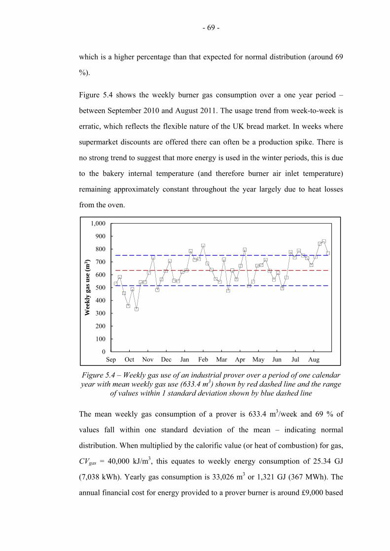
- 69 -

which is a higher percentage than that expected for normal distribution (around 69

%).

Figure 5.4 shows the weekly burner gas consumption over a one year period –

between September 2010 and August 2011. The usage trend from week-to-week is

erratic, which reflects the flexible nature of the UK bread market. In weeks where

supermarket discounts are offered there can often be a production spike. There is

no strong trend to suggest that more energy is used in the winter periods, this is due

to the bakery internal temperature (and therefore burner air inlet temperature)

remaining approximately constant throughout the year largely due to heat losses

from the oven.

Figure 5.4 – Weekly gas use of an industrial prover over a period of one calendar year with mean weekly gas use (633.4 m3) shown by red dashed line and the range

of values within 1 standard deviation shown by blue dashed line

The mean weekly gas consumption of a prover is 633.4 m3/week and 69 % of

values fall within one standard deviation of the mean – indicating normal

distribution. When multiplied by the calorific value (or heat of combustion) for gas,

CVgas = 40,000 kJ/m3, this equates to weekly energy consumption of 25.34 GJ

(7,038 kWh). Yearly gas consumption is 33,026 m3 or 1,321 GJ (367 MWh). The

annual financial cost for energy provided to a prover burner is around £9,000 based

0

100

200

300

400

500

600

700

800

900

1,000

Sep Oct Nov Dec Jan Feb Mar Apr May Jun Jul Aug

Wee

kly

gas

use

(m

3 )

- 70 -

on DECC figures of £0.0244/kWh gas (Carbon Trust, 2012b), or in the region of

1% of the capital cost (approximately £1 million). The mean power consumption of

the gas burner is 44.0 kW.

5.2.2 Air Handling Unit Electricity Consumption Trends

Distribution of air inside a prover is of critical importance to product quality and

the uniformity of the proving profile, particularly across the width of the prover,

Wz. Each loaf should be of uniform standard regardless of the position that it enters

the prover. If non-uniform air distribution across the prover width were to occur,

there would be a difference in product consistency depending on the conditions to

which each loaf is exposed. Air handling units (AHUs) are located at the loading

end of the prover and supply air via two ducts which run down the prover length,

Lx. These ducts are located either side of the centre of the prover, where the warm,

humid air is then fed into the inner volume of the prover through vents. The AHUs

generate high air pressure in the supply ducts which helps to ensure air is

distributed uniformly across the width and length of the prover.

Figure 5.5 shows the constant electricity demand of a prover AHU for the same

period as Figure 5.3, with the dip caused by downtime on Sunday when production

ceases. It can be seen by comparing Figure 5.3 and Figure 5.5 that the electricity

consumed by a prover AHU whilst operational is less variable than burner gas

consumption. This is quantified by comparing the distribution of points for

electricity consumption and gas consumption, with 95 % of values falling within

one standard deviation of the mean for electricity, as opposed to 77 % for gas. The

only values that do not fall within one standard deviation are the zero values that

occur during the shutdown period.

Figure 5.6 shows weekly electricity consumption of the prover AHU over a twelve-

month period. The mean electricity consumption is 3,747 kWh per week with 85 %

of values falling within one standard deviation of the mean – again showing the

- 71 -

low degree of weekly change in electricity consumption, which in particular

indicates that production fluctuations have little impact upon energy usage. The

total yearly consumption is 195 MWh at an annual cost of around £15,000, based

on DECC figures of £0.0755/kWh electricity (Carbon Trust, 2012b). This equates

to approximately 1.5 % of the capital cost of a prover (~£1,000,000). The mean

power consumption of the prover AHU is 23.4 kW.

Figure 5.5 – Hourly electricity use of a prover AHU over the period of one week with mean hourly electricity use (23.4 kWh) shown by red dashed line and the

range of values within 1 standard deviation shown by blue dashed line

Figure 5.6 – Weekly electricity use of a prover AHU over a period of one calendar year with mean weekly electricity use (3,747 kWh) shown by red dashed line and

the range of values within 1 standard deviation shown by blue dashed line

0

5

10

15

20

25

30

35

Saturday Sunday Monday Tuesday Wednesday Thursday Friday Saturday

Hou

rly

elec

tric

ity

con

sum

pti

on (

kW

h)

0

500

1,000

1,500

2,000

2,500

3,000

3,500

4,000

4,500

Sep Oct Nov Dec Jan Feb Mar Apr May Jun Jul Aug

Wee

kly

ele

ctri

city

con

sum

pti

on

(kW

h)

- 72 -

It can be observed that the electricity consumption is constant throughout the year,

with two slight drops in late-November and mid-July and peaks in December, May

and July. Reasons for the fluctuations in energy consumption have been suggested

by industry to be related to production levels (Price, 2012). The drops would be due

to production scheduling and/ or maintenance being carried out on the prover at

these times. The first peak in electricity consumption, which occurs in December,

has been attributed to a peak production period for a bakery due to the Christmas

holidays. The other two peaks occur in May and July, which industry suggest could

correspond to hot weather weekends during the year, when bread production tends

to increase due to more barbeques occurring. Another explanation could be high

quantities of produce required for supermarket promotions, causing a substantial

short-term increase in production.

5.2.3 Steam Consumption

Steam is injected into the prover air supply duct via a ring-main connected to a

centralised steam boiler which also provides steam to other bakery processes, as

required. Steam is automatically injected into the prover when relative humidity at

the sensor falls below the set point. Manual meter readings taken at the water

supply to the boiler over a period of one day at hourly intervals indicate that the

steam use of a prover is constant at 0.1 m3/hr of saturated steam at 8 bar (800 kPa)

pressure. Therefore, it can be calculated that the quantity of steam supplied to the

prover is 100 kg/hour (0.0277 kg/s). Using the industry standard steam tables

(Rogers and Mayhew, 1988), it can be seen that the specific enthalpy of saturated

steam at 8 bar is 2,759 kJ/kg. Using the resultant specific evaporation enthalpy, the

mean steam consumption of the prover was 76.6 kW. Given average rates of shell

boiler efficiency of 75 % (Carbon Trust, 2012a), the gas use is approximately 102.1

kW. Again, using DECC figures for cost of natural gas in the UK, £0.0244/kWh

(Carbon Trust, 2012b), and operating hours of 159 hours per week all year, the

- 73 -

annual financial cost of the portion of steam generation that is injected into the

prover is £21,000.

5.2.4 Overall Energy Usage

The total energy use of the gas burner, AHU and steam consumption is shown by

Figure 5.7, which is a culmination of the results presented in previous sections

5.2.1 to 5.2.3. The total energy use is 144.0 kW. The total yearly financial cost of

prover operation is in the region of £44,000.

Figure 5.7 – Energy utilisation profile of an industrial bread prover

In terms of CO2 emissions, the AHU (electricity) energy use has a

disproportionately high environmental impact due to the inefficiency of electricity

generation and distribution. This is highlighted by the Carbon Trust conversion

factors as shown by Table 5.1.

Fuel type Original unitEquivalent carbon impact (kgCO2e)

Electricity kWh 0.544

Natural gas kWh 0.184

Table 5.1 – Equivalent carbon impact conversion factors for electricity and natural gas (Carbon Trust, 2009)

Gas44.0 kW

26%

Electricity23.4 kW

14%

Steam102.1 kW

60%

- 74 -

Figure 5.8 shows the environmental impact of a bread prover, by converting the

primary energy use shown by Figure 5.7 into the equivalent mass of carbon dioxide

emissions using the conversion factors from Table 5.1. An energy cost profile can

provide a financial angle on the impact of energy usage – though this would be

mainly of interest to a bakery to analyse the cost efficiency of the process.

Figure 5.8 – CO2 emissions profile of an industrial bread prover

5.3 Problem Formulation

The conditions desired within a bread prover are dependent on the type of product.

Typically the relative humidity is 65 % and the temperature is 50 °C. Temperature

is controlled through modulating the fire rate of the gas burner and humidity is

controlled by the amount of steam injection. The key challenge for both prover

designers and bakeries alike is to ensure the conditions are constant across the

prover width. Currently, to ensure this is the case, provers are over-engineered with

large air handing units (AHUs) generating high pressure in the air supply, thereby

ensuring airflow is distributed more uniformly. Aside from the energy losses

relating to static pressure build-up in the ducts, the high rate of airflow means that a

Gas66938 kgCO2e

21%

Electricity105248 kgCO2e

32%

Steam155326 kgCO2e

47%

- 75 -

larger quantity of warm, humid air is expelled to the exhaust resulting in a greater

load on the gas burner and higher steam consumption.

5.4 Computational Fluid Dynamics (CFD) Model Design

Balancing temperature, humidity and air velocity distribution in three dimensions

in a complex geometry is a difficult task. It is particularly challenging to make

measurements and control conditions in a non-invasive and experimental manner.

As discussed in Chapter 4, CFD is used to analyse fluid flow numerically and is

becoming increasingly popular in the food industry, as it can be a quick, cost-

effective and non-invasive form of assessing the operational qualities of a wide

variety of food processes (Sun, 2007). Although CFD is a method that has been

applied to a wide range of food processes, including both baking and cooling

processes in the food industry, the proving of bread is a completely novel

application for this type of computational analysis (Paton et al., 2012a). CFD

allows bakers an insight into the airflow within a prover which then has the

potential to influence more energy efficient prover operation.

The aim of this study is to provide the scientific evidence to encourage the

commercial bread manufacturing industry to reduce the number of air changes in

provers via use of an experimentally validated computational model. Reducing the

number of air changes will reduce prover energy use but will also have an influence

on the proving process in terms of product quality and food safety – these factors

need to be quantified and offset to provide an energy efficient and quality-friendly

solution for industry. This is the first such study to approach prover design and

operation from a macroscopic and multi-objective perspective by use of both

computational and experimental methodologies.

CFD has been previously used in the baking industry to analyse airflows within

ovens for both energy efficiency and process optimisation (Khatir et al., 2012c,

Therdthai et al., 2004a, Verboven et al., 2000b). These techniques can be built

- 76 -

upon for the proving process for similar benefit. CFD will be used to study the

proving component of industrial bread baking for the first time as there is no

previously published work in this field.

5.4.1 Geometry

The prover analysed is a generic geometry developed by working with a

commercial prover designer, Spooner Industries Ltd., UK. The box dimensions

(refer to Figure 5.1) are: Lx = 30 m, Hy = 5 m, Wx = 5 m and Wz = 5 m. The total

prover height is 10 m. The internal volume of the prover is 311.2 m3.

Figure 5.9 – Geometry for prover CFD model generated with assistance from Spooner Industries Ltd. (Kirk, 2011)

A typical throughput for such a prover would be around 8,000 kg/hr with a proof

time in the region of 50 minutes. Air is supplied through two full length ducts with

0.2 m x 0.2 m vertical square vents distributed evenly along the prover length at 1.5

m intervals. The bread tins are modelled as solid 0.15 m x 0.56 m x 1 m blocks, and

are pitched at 1.5 m intervals. Each block represents 10 tins, referred to as ‘straps’.

Straps are attached to swings which are moved by chains to rotate the product

around the perimeter of the prover. The computational domain is shown by Figure

5.9. As the swings and chains have a negligible impact on airflow, and the velocity

- 77 -

of the tins is in the region of 0.01 m/s, the assumption is made that the straps are

stationary and floating. The arrangement of the three ducts (2 x supply and 1 x

return) can be seen by the cross section diagram in Figure 5.10. Also shown in the

diagram are the straps of tins and arrows illustrating the intended path of airflow

through the prover internal volume.

Figure 5.10 – Cross section diagram of prover showing the air ducting arrangement, location of straps of tins and blue arrows illustrating the path of

airflow

5.4.2 Turbulence Model Selection

As discussed in section 4.7, selecting a turbulence model is an important part of

CFD modelling as it allows the user to generate sufficiently accurate results whilst

ensuring that the time to compute is suitable. The intricate geometry of the prover

suggests complex flow with impinging jets of air and stagnation points close to the

walls and tins. Thus, for this application, the realisable k-ε (RKE) transport model

was chosen.

5.4.3 Boundary Conditions

The inlet conditions selected for the model range between a minimum of 10 air

changes per hour and a maximum of 100 air changes per hour, as shown in Table

Inlet duct

Inlet duct

Return duct

- 78 -

5.2. The Reynolds number for each case is shown, based on characteristic length

scale, Lc = 0.5 m.

Case number Number of air changes, N (/hr)

Inlet velocity, uin (m/s)

Reynolds number at inlet, Re

1 10 1.73 51,003 2 20 3.46 102,007 3 30 5.19 153,010 4 40 6.92 204,014 5 50 8.64 255,017 6 60 10.37 306,021 7 70 12.10 357,024 8 80 13.83 408,028 9 90 15.56 459,031 10 100 17.29 510,035

Table 5.2 – Inlet boundary conditions for prover CFD model

Figure 5.11 – Partial view of prover CFD solution domain showing boundary conditions and symmetry plane

The BCs and symmetry plane can be seen in Figure 5.11. The loading and

unloading space is often covered with an air curtain which is brushed aside when

tins pass through, and therefore there is no suitable BC to be applied. The model is

three-dimensional and utilises a symmetry plane to reduce the processing time. The

number of air changes is driven by the inlet air velocity, uin, which is a BC located

0.5 m from the loading end on the top surface of the centre of the supply duct. The

Patm

uin

Symmetry plane

- 79 -

outlet vent, which allows flow into the outlet duct, is in the centre of the return

duct. The BC for the pressure outlet, Patm, is located co-planar to the inlet.

5.4.4 CFD Solution Process

The mesh was unstructured and generated using the ANSYS Workbench meshing

tool, which uses the Finite Volume Method. Tetrahedral elements were used and

the maximum element edge length was set at 0.05 m. Mesh refinement was

specified in the areas close to the inlet and outlet at a maximum of half the element

size of the rest of the prover, as this is where the highest degree of turbulence was

expected. As the temperature was close to ambient and temperature fluctuations

within the prover were considered negligible, the solution domain was assumed to

be isothermal. Turbulence intensity at the inlet was set at 10 %, assuming a high

degree turbulent flow due to the large velocity magnitude and length scale was

selected as 0.0175 m based on guidance from the ANSYS User’s Guide (ANSYS

Inc., 2009). The solution was considered converged once the continuity, x/ y/ z

velocity, k and ε residuals reached 10-5, which took approximately 24 hours for

each case using a desktop PC.

5.5 Theory of Residence Time Distribution Analysis

Residence time theory was originally developed by chemical engineers to quantify

the degree of mixing of fluids inside fluid vessels. The seminal paper on residence

time distribution analysis describes flow distribution in mixing tanks through C-

diagrams and F-diagrams (Danckwerts, 1953). F-diagrams give the fraction of the

fluid flow that is mixed at the outlet with respect to time, whilst C-diagrams display

the concentration of injected particles at the outlet with respect to time. For this

study, C-diagrams are of more use as humid air is already mixed by the time it

enters the prover and more important than the degree of mixing is identification of

stagnation regions in the flow. A diagram of a mixing tank for illustration of the

physical meaning of a C-diagram is shown by Figure 5.12.

- 80 -

Residence time is important to bread proving as it is directly related to the number

of air changes per hour, N, which is the control that industrial bakeries use to

ensure the processes meet their own strict criteria as well as important legislative

constraints regarding food safety and health, safety and the environment (HSE). It

is recommended that bakeries have air changes of at least 20 per hour (Brumbaugh,

2011). The greater the number of air changes, the lower the mean residence time.

This results in more energy losses as a result of replacing warm, humid air that has

been exhausted to atmosphere and more electricity used by high fan loads.

Figure 5.12 – Diagram of a mixing tank showing the concentration of the particles injected at the inlet (A) at the outlet (B) with respect to time

C-diagrams for four representative flow types are shown by Figure 5.13. These four

residence time distribution curves can describe most types of regular flow inside a

vessel, although in reality fluctuations occur due to irregularities within the fluid

domain. Figure 5.13 (a) shows piston flow, which is not possible for Newtonian

fluids due to viscosity – for this prover example it would mean that all the flow

exits the prover after the same amount of time. Piston flow with some longitudinal

mixing, shown by Figure 5.13 (b), is realistically the best case scenario for flow

within a prover, as it means all the flow exits the prover within a small space of

time. This ensures the flow is well mixed and there are no stagnant zones of

A B

C(t)

- 81 -

recirculation. Figure 5.13 (c) and (d) show two types dispersed flow. Figure 5.13

(c) is described as perfect-mixing which indicates immediate dispersal of particles

upon injection to the volume. Figure 5.13 (d) shows dead water which is

undesirable in a food production environment as it causes stagnation regions which

can affect both food safety and product uniformity.

Figure 5.13 – C-diagrams as described by Danckwerts (1953) for: (a) piston flow (b) piston flow with longitudinal mixing (c) complete mixing and (d) dead water

The profile of the residence time distribution curve can be characterised by the exit

age residence time function E(t), which is the quantity of fluid that has been in the

system for between t and t + dt seconds (Coker, 2001).

In order to generate a residence time distribution curve for airflow using

commercial CFD software, ANSYS Fluent has a particle tracking feature which

injects a set number of massless, sizeless ‘particles’ into the flow and tracks the

path of each one at a set time step and range (ANSYS Inc., 2009). The number of

particles passing through the outlet boundary after each time step can be extracted

from the software. The time step associated with the particle escaping through the

(a) (b)

(c) (d)

C(t) C(t)

C(t) C(t)

100 % 100 %

t t

t t

100 % 100 %

- 82 -

outlet can be termed ‘residence time’ and therefore a distribution of residence time

can be plotted.

5.6 Verification and Validation of Computational Model

Verification of the CFD model is performed via a mesh sensitivity analysis, where

the minimum size of the mesh for reliable results is determined. In addition, an

experimental validation of the air velocity through the prover air vents is

conducted.

5.6.1 Verification of Mesh Generation

The size of mesh (or the number of elements) in a CFD geometry affects the

accuracy and processing time of a computational problem. It is important to have a

fine enough mesh to achieve sufficient resolution of results without wasting

computing resources. Figure 5.14 shows the velocity profile across a prover vent

for different numbers of elements.

Figure 5.14 – Velocity profile across a single prover vent, the second closest to the loading/ unloading end, for five different mesh sizes/ numbers of elements

It can be observed that the profiles for 9.20 x 104 and 3.39 x 105 elements have

qualitatively less accurate velocity profiles when compared to the case with 1.39 x

106 elements, thus implicating strong dependency of the solution on the mesh for

0

1

2

3

4

5

6

7

8

2.9 3.0 3.1 3.2 3.3 3.4

Air

vel

ocit

y (m

/s)

Distance along prover (m)

91,973

339,216

614,358

1,000,262

1,391,262

Number of elements

9.20 x 104

3.39 x 105

6.14 x 105

1.00 x 106

1.39 x 106

- 83 -

these two cases. The overall correlation between the vent velocity profiles is

calculated by Pearson’s r coefficient and is shown by Figure 5.15 for the five

different mesh sizes. The minimum value of r has been set at 0.975 to ensure

quantitative validation. The two coarser meshes shown by Figure 5.14 of 9.20 x 104

and 3.39 x 105 elements had r values of 0.792 and 0.963. Again, it is shown that

meshes with more than ~6 x 105 elements have sufficient statistical correlation (r =

0.978) combined with the qualitative agreement shown by Figure 5.14 to be used

for analysis. Calculation time for the model with 6.14 x 105 elements was

approximately 6 hours. This mesh size has satisfactory velocity profile accuracy

and a realistically viable processing time and therefore this mesh was selected.

Figure 5.15 – Pearson’s r correlation showing correlation with the finest mesh case (1.39 million cells) for velocity profile across a single prover vent

5.6.2 Experimental Validation

Experimental validation of the CFD analyses was carried out by measuring the air

velocity at each outlet vent within an industrial prover. The experiments were

conducted using a calibrated Testo 405 Thermal Anemometer (Testo Limited, UK).

The accuracy given by the original equipment manufacturer (OEM) was ± 0.3 m/s

+ 5 % of maximum velocity. The velocities measured were in the region of 3.3 to

0.0

0.2

0.4

0.6

0.8

1.0

000 250,000 500,000 750,000 1,000,000 1,250,000 1,500,000

Pea

rson

pro

du

ct-m

omen

t co

rrel

atio

n

Number of elements

- 84 -

10.0 m/s therefore the readings could be assumed with an accuracy of within ± 0.8

m/s, giving a percentage error of between 8.00 and 24.24 %.

The experimental measurements of mean air velocity from each duct are compared

to the computational predictions in Figure 5.16. A good degree of validation can be

inferred from these measurements, with a mean percentage difference of 7.50 %

and a Pearson correlation value of r = 0.798. The correlation is particularly evident

in the half of the prover closest to the loading end, x < 15 m, as flow in this region

appears to be better predicted by CFD – the mean percentage difference between

experimental results and computational predictions was 5.30 %.

Figure 5.16 – Validation of velocity profile along prover length with error bars representing the experimental error relating to the apparatus used

5.7 Results

The results of CFD can be displayed visually (for example contour plots of air

velocity) and numerically (in the form of graphs, tables etc.).

5.7.1 Plots of Velocity Distribution

This section presents results in the form of contour plots and velocity vector plots

of air velocity, where yellow/ red colours show high velocity and cyan/ blue

0

2

4

6

8

10

12

0 5 10 15 20 25 30

Air

vel

ocit

y (m

/s)

x-position along prover (m)

CFD resultsExperimental data

- 85 -

colours represent areas of low velocity. A 3D contour plot of air distribution within

the prover volume is shown by Figure 5.17. Nineteen planes normal to the x-axis

are shown – one representing each pair of vents on the inlet duct. This plot gives an

overall view of velocity distribution through each vent along the length of the

prover. High air velocity is evident close to each air vent but especially for the

vents in the centre of the prover, whereas low air velocity can be seen towards the

loading and unloading areas in the prover and around the straps in the first quarter

of the prover. These areas of low air velocity indicate dead regions of stagnant air

and can have three particularly adverse effects for bakeries:

(i) Lower rates of heat transfer to the product as the rate of convective heat

transfer is proportional to air velocity.

(ii) Less uniform air temperature and humidity.

(iii) Lower air temperature and air velocity, as the stagnant air may cool

down and the moisture may condense as it is replaced less often.

Figure 5.17 – Isometric view contour plot of air velocity illustrating air distribution throughout the prover volume

Figure 5.18 shows the same planes down the prover length from a top view. This

contour plot highlights the degree of velocity uniformity at each vent. It can be

seen that the air velocity through the central vents in the x-direction are larger than

the velocities at both extremities. In addition, the effect of the interaction between

- 86 -

the air jets from the vents and the inside of the prover walls is shown, with air

appearing to be artificially steered downwards towards the tins by the right-angled

prover geometry. An inner geometry more conducive to directing flow towards the

tins could be more applicable in this instance and would make an interesting

parametric study with regards to optimising this airflow and assessing the

associated additional manufacturing and cleaning costs.

Figure 5.18 – Angled top view contour plot of air velocity showing air distribution down the prover length

The velocity vector plot shown by Figure 5.19 shows the path and magnitude of air

through a representative plane parallel to the yz-axis. The high magnitude of air

velocity near to the vent illustrates the high degree of turbulence that is present in

this area. Furthermore, the comparatively low airflow around the tins that is caused

by the prover design with vents facing away from the product. This ensures that the

delicate dough is not subjected to high-velocity air jets, which could cause the air

cells within the dough to collapse. The vector plot shows that is some substance to

- 87 -

the assumption of prover designers that air deflects off the inside walls of the

prover towards the product.

Figure 5.19 – Velocity vector plot of air velocity showing flow paths of air through a prover vent and around the product for the 13th plane parallel to a vent from the

loading end

Figure 5.20 shows contour plots of velocity distribution around the tins for two

planes perpendicular to the x-axis: (a) parallel to the vent closest to the loading end

and (b) parallel to the 13th vent from the loading end. The range of air velocity

shown is reduced to 0 < u < 0.8 m/s allowing further resolution to be shown for

areas of low velocity – i.e. to enhance the visualisation of flow around the product.

Contour plots of air velocity show similar trends for each of the 19 planes

positioned in the centre of an inlet vent down the prover length. Figure 5.20 (a)

shows explicitly the regions of low air velocity between the lower tins, indicating

stagnation regions at the loading and unloading end of the prover, corroborating the

conclusions drawn from Figure 5.17. This will not be a major concern for prover

designers, as airflow is deliberately minimised near the loading and unloading ends

of the prover to prevent heat and humidity losses to atmosphere. However, it is

important to maintain airflow around the tins in the main sections of the prover – in

the region shown by Figure 5.20 (b), which demonstrates undesirable stagnation

regions above the upper straps and below the lower straps, though this is somewhat

mitigated by the uniformity of airflow in between the straps of tins. Both contour

- 88 -

plots also illustrate the interaction between the prover air jets and the wall where

prover designers intend to deflect air off the prover wall towards the product.

(a)

(b)

Figure 5.20 – End-on view contour plot of air velocity showing airflow distribution around the tins for (a) the plane closest to the loading end, and (b) the 13th plane

from the loading end

5.7.2 Numerical Results

The red line shown by Figure 5.21 is parallel to the xy-axis and in offset from the

outlet vents by 5 mm. The air velocity distribution profile down the prover length

on this line is shown by Figure 5.22. It is clear to see the peaks of u > 4 m/s at for

each of the 19 vents 1.5 m intervals along the prover. The peaks are of different

- 89 -

magnitudes due to uneven air distribution through the supply duct. Modifying the

internal geometry of the supply duct to force more air through the first three ducts

would improve the uniformity of velocity, but may also force more air out of the

loading/ unloading areas of the prover and thus contribute towards energy losses.

The modification in geometry could be as simple as a decreasing cross section with

x which would increase the relative total pressure towards x = 0 m and force higher

velocities for these vents.

Figure 5.21 – Prover section view from perpendicular to the xy-plane with red line passing through the centre of the air vents offset in the z-direction by 5 mm

Figure 5.22 – CFD predictions showing the air velocity profile along the prover length for the red line shown in Figure 5.21

5.8 Residence Time Distribution Curves

Residence time distribution curves can be used to verify whether or not the number

of air changes is suitable for production purposes. By tracking individual particle

flow paths, it is possible to examine overall characteristics of the airflow. If a high

0

1

2

3

4

5

6

7

8

0 5 10 15 20 25 30

Air

vel

ocit

y (m

/s)

Distance along prover (m)

- 90 -

proportion of particles take a long time to escape through the pressure outlet there

is a greater chance of a breach in quality standards. The specific standards have not

yet been specified quantitatively by a regulatory body; therefore the results of this

study could be used to guide future standards for the proving process of bread

manufacture.

A typical graph showing the residence time distribution for five cases is shown by

Figure 5.23. This illustrates the time taken for each one of 2,469 particles to escape

the prover cavity through the outlet after a maximum of 360 seconds. The particles

are introduced at the inlet at equally spaced intervals. For all cases, the majority of

particles exit the prover within 100 seconds. However, a small proportion of

particles have a longer residence time indicating the presence of dead regions and

stagnation zones within the flow. More positively skewed residence time

distributions will reduce the possibility of mould spores occurring inside the

prover, since this shows less proportion of particles stagnating.

Figure 5.23 – Residence time distribution for 2,469 particles

Mean residence time is of limited use to industry as it does not give an indication as

to the residence time distribution spread, which means the prover operator will

have little idea as to the portion of air that is stagnant and poses a food quality or

0%

5%

10%

15%

20%

25%

30%

0 20 40 60 80 100 120 140

Per

cen

tage

of

par

ticl

es

Residence time (s)

100 air changes per hour





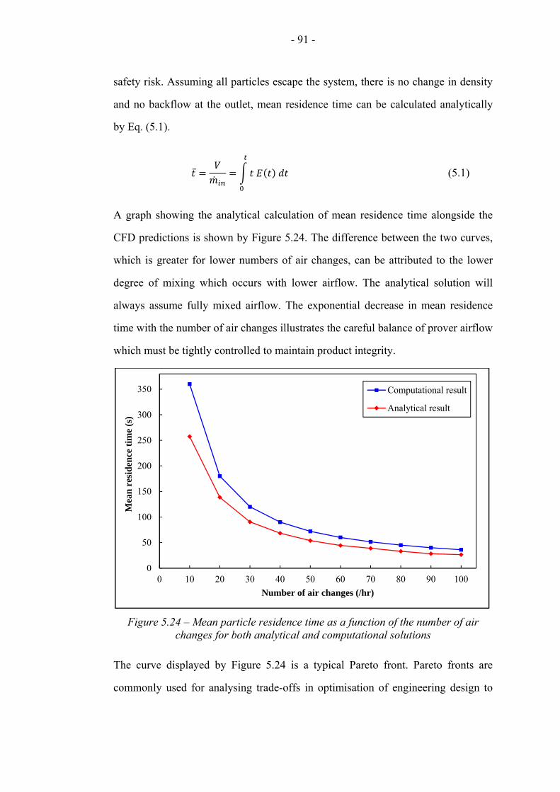
- 91 -

safety risk. Assuming all particles escape the system, there is no change in density

and no backflow at the outlet, mean residence time can be calculated analytically

by Eq. (5.1).

(5.1)

A graph showing the analytical calculation of mean residence time alongside the

CFD predictions is shown by Figure 5.24. The difference between the two curves,

which is greater for lower numbers of air changes, can be attributed to the lower

degree of mixing which occurs with lower airflow. The analytical solution will

always assume fully mixed airflow. The exponential decrease in mean residence

time with the number of air changes illustrates the careful balance of prover airflow

which must be tightly controlled to maintain product integrity.

Figure 5.24 – Mean particle residence time as a function of the number of air changes for both analytical and computational solutions

The curve displayed by Figure 5.24 is a typical Pareto front. Pareto fronts are

commonly used for analysing trade-offs in optimisation of engineering design to

0

50

100

150

200

250

300

350

0 10 20 30 40 50 60 70 80 90 100

Mea

n r

esid

ence

tim

e (s

)

Number of air changes (/hr)

Computational result

Analytical result

- 92 -

minimise a particular cost (in this case energy) whilst maintaining minimum

standards (in this case product quality and food safety).

5.9 Energy Savings

The stagnation of particles (for example as seen in Figure 5.20 in the loading/

unloading area of the prover) is emphasised by the number of particles remaining

in the prover after 360 s, as shown by Figure 5.25. Bakers do not typically know

the maximum percentage of particles that should have escaped after 360 s, but

these results help to give confidence to prover operators when reducing the number

of air changes in order to reduce the energy consumption of the prover. It has been

suggested by industrialists that less than 1 % of particles remaining inside the

prover cavity after 360 s may be an initial estimate to work with, which would

immediately enable bakers to initially reduce the number of air changes from 90/hr

to 60/hr (Price, 2012).

Figure 5.25 – Percentage of particles not escaped the prover cavity after 360 s residence time for each case

With current design, the easiest way to eradicate high residence time is to increase

the number of air changes. Equally, for energy savings, adjustment of the AHU to

0%

5%

10%

15%

20%

0 10 20 30 40 50 60 70 80 90 100

Per

cen

tage

of

par

ticl

es n

ot e

scap

ed

Number of air changes (/hr)

- 93 -

reduce the number of air changes will reduce the steam, gas and electricity demand

of the prover. A reduction in the number of air changes from 90/hr to 60/hr

potentially means significant energy savings for the bread industry. Bakeries are

trialling this decrease at present as a result of this work and therefore it is too early

to prove the year-on-year energy savings based on a full regression analysis.

However, engineering estimates of the reduction in electrical load based on theory

are possible. Firstly, the quantity of air to be moved by the fans will be 33 % less.

By relating this to the power law of fan energy consumption, Eq. (5.2), the required

energy can be calculated from the pressure difference between the duct and baking

chamber:

∆ ∆ (5.2)

where the pressure difference, ΔP (Pa), is calculated by the required inlet velocity

by using Bernoulli’s equation, Eq. (5.3):

12

(5.3)

Therefore, if the inlet velocity is reduced by 33 %, the fan power required would be

reduced by over 70 %. Gas and steam use will also be lower as a result of a

reduction in the number of air changes. However, quantifying these in generic

terms is not practical as it depends greatly on the degree of recirculation of air at

the return duct specified by individual bakeries.

5.10 Summary

This CFD study has allowed a large amount of quantitative data to be collected

without the need for time consuming and expensive experimentation. A generic

prover geometry design was developed alongside industrial prover manufacturers

to predict isothermal airflow. A parametric study was conducted by varying the

number of air changes 10/hr and 100/hr, which are conditions that are realistically

feasible for industrial bread proving.

- 94 -

The model has been experimentally validated by measuring air velocity inside an

operational prover. The results collected from the CFD model showed strong a

correlation with the equivalent measurement points. A mesh sensitivity analysis

was performed in order to verify the model, and the element-size beyond which the

results converged was identified.

Residence time distribution theory was used to quantify the distribution of number

of particles escaped after each time step with respect to the number of air changes

which has enabled bakeries to make informed choices about reducing the number

of air changes to reduce the energy cost. It has been suggested that the number of

particles not escaped after 360 seconds could be used by regulatory bodies to give a

quality standard for food safety in the bread proving process to measure the

probability of mould spores developing.

The results suggest there is scope to reduce the number of air changes, depending

on the product quality specifications dictated by the bakery. The number of

particles that remain in the prover after 360 s of being injected is less than 1 % for

N ≥ 60. A reduction from 90 to 60 air changes per hour represents a 33 % reduction

in prover airflow. Savings in electricity for this reduction have been estimated at

over 70 %. Gas and steam savings are likely to be made possible as a result – a

regression analysis would be required to accurately quantify the energy impact of

such changes.

- 95 -

Chapter 6

System-Level Thermodynamic Analysis

of Commercial Bread Baking Ovens

As shown by previous reports and authors, ovens use half of the energy consumed

in the bread manufacturing process (Carbon Trust, 2010, Thumann and Mehta,

2008). It is naturally an area of interest for bakeries to reduce carbon emissions and

energy costs. This chapter provides a methodology for modelling baking oven

energy use. This system-level model has been widely used in industry to

benchmark current ovens, and to identify areas for oven manufacturers to invest in

new design in order to improve efficiency of current machinery. The methodology

of this system modelling approach has been presented at the Sustainable Thermal

Energy Management International Conference 2011 (Paton et al., 2011) and

published in Applied Thermal Engineering (Paton et al., 2012b).

The overall aim is to show how a methodology can be developed to drive forward

equipment design and influence operating conditions in order to improve energy

efficiency of bread baking ovens. The overall methodology enables the most

promising opportunities for achieving significant reductions in carbon footprint and

financial running cost that can benefit the baking industry to be assessed.

6.1 Oven Configurations

There are two main types of continuous tunnel ovens used in large industrial

bakeries; direct-fired and indirect-fired. The important distinction between these

two configurations relates to whether combustion products enter the baking

chamber. For direct fired ovens the products of combustion do enter the baking

chamber, whereas for indirect ovens the products of combustion remain separate

from the baking chamber and heat is introduced to the surface of the bread via heat

exchangers. Forced convection and ribbon burner are two types of direct-fired

ovens. Radiant and turbo-radiant are two types of indirect ovens used in the

- 96 -

commercial baking industry. The differences between direct and indirect ovens are

illustrated schematically by Figure 6.1:

(a)

(b)

Figure 6.1 – Schematics of two different oven designs: (a) direct-fired forced convection and (b) indirect-fired radiant

Ovens are typically gas, oil or electrically powered. Heat transfer systems include

infrared, forced convection, radiation and halogen-lamp. Over the years alternative

oven designs have been investigated, such as microwave oven technology (Norris

et al., 2002) and hybrid ovens (Li and Walker, 1996).

Recirculation fan

Product

Bottom nozzle bank

Top nozzle bank Exhaust

fan

Exhaust damper

Fresh air inlet

Burner

Exhaust fan

Fresh air inlet

Burner

Exhaust damper Radiation

tubes

Product

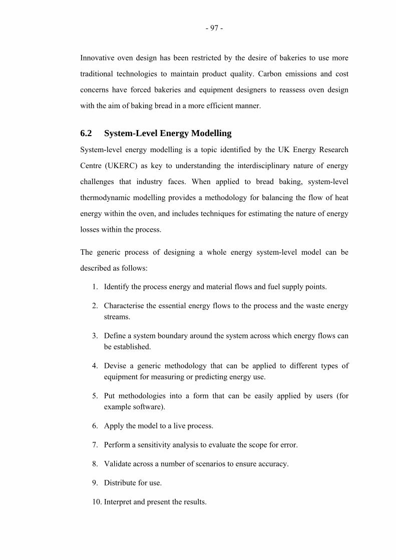
- 97 -

Innovative oven design has been restricted by the desire of bakeries to use more

traditional technologies to maintain product quality. Carbon emissions and cost

concerns have forced bakeries and equipment designers to reassess oven design

with the aim of baking bread in a more efficient manner.

6.2 System-Level Energy Modelling

System-level energy modelling is a topic identified by the UK Energy Research

Centre (UKERC) as key to understanding the interdisciplinary nature of energy

challenges that industry faces. When applied to bread baking, system-level

thermodynamic modelling provides a methodology for balancing the flow of heat

energy within the oven, and includes techniques for estimating the nature of energy

losses within the process.

The generic process of designing a whole energy system-level model can be

described as follows:

1. Identify the process energy and material flows and fuel supply points.

2. Characterise the essential energy flows to the process and the waste energy streams.

3. Define a system boundary around the system across which energy flows can be established.

4. Devise a generic methodology that can be applied to different types of equipment for measuring or predicting energy use.

5. Put methodologies into a form that can be easily applied by users (for example software).

6. Apply the model to a live process.

7. Perform a sensitivity analysis to evaluate the scope for error.

8. Validate across a number of scenarios to ensure accuracy.

9. Distribute for use.

10. Interpret and present the results.

- 98 -

A full scale energy audit is often useful for industry to identify inefficient processes

and make improvements; however these are often time consuming, costly, and give

unnecessarily convoluted results in order to analyse a complete system. Although a

system-level model will often encompass key components of an energy audit, the

main aim is to include flexibility so it can be applicable to a number of scenarios

without significant modification. The main benefit of system-level models is that

they provide useful results to justify process improvements, whilst remaining cost

effective and time efficient.

6.3 Theory of Energy Audits

There are a number of books that describe energy auditing techniques for industrial

processes (Beggs, 2002, Gottschalk, 1996, Hansen and Brown, 2004, Kreith and

Goswami, 2008, Marcotte and Grabowski, 2008, Mattsson and Sonesson, 2003,

Thumann and Mehta, 2008, Thumann and Younger, 2003, Turner, 1993). These

authors all outline practical techniques for quantifying energy streams in

manufacturing processes, buildings and transportation systems. Turner (1993)

describes the drivers for energy auditing as “to ensure survival, maximise profits,

and enhance competitive positions”.

Thumann and Mehta (2008) give a comprehensive description of industrial energy

audits with a focus on site services and process optimisation, including: HVAC,

lighting, electricity co-generation, heat recovery, control systems and thermal

storage. In addition, transportation and envelope audits were discussed. Two phases

are listed; “acquisition” and “analysis of data”, the results are then used to develop

savings opportunities. There are a number of methods for analysing energy savings

proposals over the life time of an installation. Such models are sensitive to

changing fuel prices and economic circumstances giving an overall value to a

business in terms of payback time. If the payback is deemed economically

beneficial and installation is practical, priorities for investment proposals can be

- 99 -

made. It is important to continuously monitor and record energy consumption

through use of submetering after changes have been introduced, in order to ensure

performance is improved to the levels predicted.

A large focus of Thumann and Mehta (2008) is on the worldwide legislation that

has been brought into effect over recent years. There is a detailed analysis of

different system measurement techniques and devices, of particular interest was the

use of infrared thermal imaging to analyse heat losses. Heat recovery options are

assessed – the process of directing waste heat streams through a heat exchanger, or

otherwise, to reduce the energy losses in flue gases. For heat recovery purposes,

heat from oven exhaust gasses can be categorised as within the low temperature

range, i.e. less than 232 °C. This means heat recovery would not typically involve

conversion of heat to mechanical power (for example Stirling engines), due to

inefficiencies involved with low grade heat, but instead pre-heating fluid streams

such as feed water. There are a variety of commercially available heat exchangers,

which are explained and analysed for their functionalities.

Beggs (2002) described the audit process in four stages:

(i) collation of data

(ii) analysis of data

(iii) presentation of energy consumption

(iv) assess priorities for energy efficiency savings

The first three stages are the main processes necessary to establish the basic

framework and strategy for energy usage and reduction. The fourth stage can be

used to make necessary recommendations for detailed energy savings proposals.

This is followed by a financial appraisal, using two different valuation techniques:

“net present value” and “internal rate of return”. A cautious approach is advised for

new installations; the author warns that the cost of running ancillary equipment,

such as fans and pumps, could outweigh the financial and environmental benefit

- 100 -

gained through recovering waste heat. There is a comprehensive guide to heat

exchangers and heat pumps, covering all the main flow types used in industry.

Much of the book is relevant to supply of site services, cogeneration and building

design. Overall, this book is a reliable reference from which to conduct an energy

audit.

6.4 System-Level Model of a Commercial Baking Oven

The methodology presented here is generic; therefore it can be applied to any type

of large production oven. The analysis was illustrated and validated for a standard

800 g white loaf, though when applying this model practically the type of product

being manufactured makes very little difference to the overall results of the model.

The quantity of ingredients as a percentage of the weight of the while loaf recipe is

(as a percentage of initial dough mass): 55.7 % flour, 1.1 % salt, 4.2 % yeast, 2.8 %

sugar, 30.6 % water and 5.6 % other ingredients (Monteau, 2008). The model

generated assumes steady-state operating conditions – an assumption that is

justified given the continuous nature of bread baking operations.

Several methodologies have been proposed for analysing the thermodynamic

energy flows in processing equipment, according to the First Law of

Thermodynamics. These methods combine a number of techniques outlined by

energy audit books and aspects of pinch analysis as well as offering some novel

approaches for quantifying heat losses (Wu et al., 2010, Wu et al., 2012).

After surveying a number of industrial bread ovens and bakeries, it was possible to

summarise the energy functions of a bread oven into ten key heat flows. There are

two heat supply methods: heat in via the gas burner and steam injection. There are

seven areas where the thermal energy is utilised or dissipated: cooking of the

dough, evaporation of water from the product, starch gelatinisation, heat uptake of

tins and lids, heat in exhaust gases, heat uptake of the conveyor and losses through

the oven walls and roof. These are summarised in Figure 6.2 and Table 6.1.

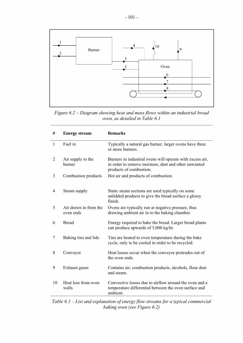
- 101 -

Figure 6.2 – Diagram showing heat and mass flows within an industrial bread oven, as detailed in Table 6.1

# Energy stream Remarks

1 Fuel in Typically a natural gas burner, larger ovens have three or more burners.

2 Air supply to the burner

Burners in industrial ovens will operate with excess air, in order to remove moisture, dust and other unwanted products of combustion.

3 Combustion products Hot air and products of combustion.

4 Steam supply Static steam sections are used typically on some unlidded products to give the bread surface a glossy finish.

5 Air drawn in from the oven ends

Ovens are typically run at negative pressure, thus drawing ambient air in to the baking chamber.

6 Bread Energy required to bake the bread. Larger bread plants can produce upwards of 5,000 kg/hr.

7 Baking tins and lids Tins are heated to oven temperature during the bake cycle, only to be cooled in order to be recycled.

8 Conveyor Heat losses occur when the conveyor protrudes out of the oven ends.

9 Exhaust gases Contains air, combustion products, alcohols, flour dust and steam.

10 Heat loss from oven walls

Convective losses due to airflow around the oven and a temperature differential between the oven surface and ambient.

Table 6.1 – List and explanation of energy flow streams for a typical commercial baking oven (see Figure 6.2)

10 9

6

7

8

1

2 3

4

5

Burner

Oven

- 102 -

The governing methodology, measurement techniques and related equations used

to define the heat flows into and out of a bread oven are summarised in sections

6.4.1 to 6.4.8.

6.4.1 Heat in via Gas Burner

The amount of energy supplied to the oven from the burner (Figure 6.2, flow 3) is

calculated from the volumetric flow rate of fuel used in each of the three burners,

multiplied by the calorific value of the natural gas. Because the supply air for oven

gas burners is not typically preheated, the heat injected to the baking chamber

through the gas burner is shown by Eq. (6.1).

∙ (6.1)

where is the heat flow (kW) and is volumetric flow rate (m3/s). The heat of

combustion for natural gas, CVgas (J/m3), is supplied at 25 °C. The average

temperature in a bakery is typically between 24 and 30 °C. In this temperature

range, CVgas varies by less than 0.03 %; therefore the assumption that burner inlet

air is temperature is 25 °C is suitable for this model.

6.4.2 Heat in via Steam Injection

Some baking processes require the injection of steam at the start of baking (flow 3),

as bakers believe the condensed moisture on the top surface of the bread gives it a

glossy (or glazed) finish (Altamirano-Fortoul et al., 2012). For these particular

products, energy in via steam injection can be represented by Eq. (6.2). This

equation takes into account the mass flow rate of steam and the evaporation

enthalpy of water.

∙ (6.2)

where is mass flow rate (kg/s) and is is specific heat at constant pressure

(J/(kg·K)) and the subscript w represents water. The latent heat of evaporation for

water, Lew, at atmospheric pressure is 2,260 kJ/kg at 100 °C (Bird and Ross, 2012).

- 103 -

6.4.3 Heat Required to Cook the Dough

The heat required to cook the dough is given by the difference between the heat in

the product at the end and at the beginning of the baking process (flow 6). This is

calculated using Eq. (6.3):

∙ ∙ (6.3)

In addition, heat is required to gelatinise the starch within the dough, an irreversible

process that is characterised by starch molecules absorbing water and setting the

dough to create bread – thereby essentially defining the baking process (Fessas and

Schiraldi, 2000). Starch gelatinisation is important for three reasons:

(i) it provides an indication of when the bread is cooked

(ii) it forms the dough together to create the crumb structure inside the loaf, and

(iii) it controls the rate of the staling process of the bread (Yasunaga et al., 1968).

The heat required for starch gelatinisation is calculated by Eq. (6.4):

∙ (6.4)

where specific heat of starch gelatinisation, cgel = 1.2 kJ/kg baked product (Le-Bail

et al., 2010).

Assuming a constant temperature on the bread surface at the start of the baking

process, the rate of temperature increase inside the dough/ bread can be modelled in

a simplified manner by Eq. (6.5):

∆1

(6.5)

Thermal diffusivity is given as a function of temperature (αk), assuming a constant

dough/ bread density as obtained from Wong et al. (2007) – this is also shown in

Figure 3.1. Zanoni et al. (1995b) developed a model to evaluate the degree of

starch gelatinisation to predict the rate at which the bread is baked, Eq. (6.6):

- 104 -

1 (6.6)

where α(t) is the degree of gelatinisation. The reaction rate constant, Kr, is

calculated in terms of the Arrhenius equation:

(6.7)

where the pre-exponential factor, K0, is 2.8 x 1018/s and the activation energy, Ea =

139 kJ/mol. These equations have been used to develop a computational model for

the prediction of bread temperature and the degree of starch gelatinization with

respect to bake time (Khatir et al., 2012b).

6.4.4 Heat Required for Moisture Evaporation

The mass of moisture evaporated from the dough (flow 9) during baking is highly

dependent on the product type, oven type and baking process. The heat required for

evaporation is mostly due to the latent heat, as discussed in section 3.5. The system

model uses Eq. (6.8) to calculate this energy load:

, ∙ (6.8)

6.4.5 Heat Uptake of the Tins and Lids

When the dough is transferred to the tin it is in a delicate state so recycled tins are

often cooled to ambient temperature after the bake cycle to prevent scorching of the

dough. Additionally, many products use lids which are useful to create a

microclimate of moist air within the tins. The lids also control the shape of the top

of the loaf as the dough expands. The energy required to heat the tins and lids (flow

7) is given by Eq. (6.9):

, , , , , , ∙ (6.9)

tins lids

- 105 -

6.4.6 Heat Uptake of the Oven Conveyor

Conveyors in industrial ovens (flow 8) are typically large steel slats covered in a

steel mesh to support the bread travelling through the oven. The mass flow rate of

the slats is typically comparable to that of the mass flow rate of bread travelling

through the oven, although feed and return temperatures are closer to the set point

of the oven, due to the high thermal conductivity of steel – approximately 30 to 40

W/(m·K), depending upon the exact grade (Kreith et al., 2011). The heat loss of the

conveyor is calculated by Eq. (6.10):

∙ (6.10)

6.4.7 Heat in the Flue Gas

The exhaust flue (flow 9) mostly consists of hot air, water vapour and combustion

products removed from the baking chamber. Other components such as grease and

flour are neglected for the purposes of calculations. The flow rate of flue gas was

measured using a pitot tube inserted into the exhaust duct. Measurements ideally

should be completed at traverse points located at equal increments across the duct

and averaged to obtain the most stable value. The mass flow rate is then used to

calculate the heat losses from flue gases by using Eq. (6.11):

, , ∙ (6.11)

where the simplification that specific heat of the exhaust gases is the same as the

specific heat of air, cPair, as oven burners are purposely set to operate with large

amounts of excess air (typically greater than 50 %).

Hood exhausts are often positioned at the oven entrance and exit to extract hot air

and combustion product to prevent these gases entering the bakery atmosphere.

Hood exhaust gases are much lower in temperature than exhaust gases. Where

relevant, these gases should also be included in flue gas energy loss calculation. In

- 106 -

order to do this, the quantity of fresh air and air that has over spilled from the oven

should be quantified – which can be estimated by analysing the comparative

temperature between ambient and the baking chamber. The fresh air that is

exhausted from the oven should then be deducted from the total mass flow rate.

The lower exhaust gas temperature can then be used in Eq. (6.11).

6.4.8 Heat Loss from Oven Walls and Roof

Heat losses from the surface of an oven (flow 10) are dependent on the surface

temperature, ambient air temperature and airflow near the surface of the oven. To

estimate the surface temperature, a thermal imaging camera was used

(ThermaCAM™ SC640, FLIR Systems Ltd, UK), and validated using a surface

thermocouple probe – more details are given in section 6.5. The convective heat

losses through the vertical stainless steel oven walls were estimated using Eq.

(6.12):

(6.12)

where heat transfer coefficient, h (W/(m2·K)), is calculated from the Nusselt

number:

∙

(6.13)

where λ is thermal conductivity (W/(m·K)). The Nusselt number, Nu, is highly

dependent on the atmospheric conditions around a flat surface. Therefore, the

Nusselt number is different for the vertical oven wall panels and the horizontal

pressure relief panels situated on the oven roof.

A correlation for heat transfer from the surface of vertical walls has been outlined

by Incropera and DeWitt (2007) and is given by Eq. (6.14):

43∙

4

.

(6.14)

- 107 -

where the Grashof number and the Prandtl number are both commonly defined

dimensionless numbers used in a range of fluid dynamics and heat transfer

problems. The Grashof number is the ratio of buoyancy to viscous forces in a fluid

and the Prandtl number is ratio of kinematic viscosity to thermal diffusivity in a

fluid.

Heat transfer from the surface of horizontal pressure relief panels located on the

oven roof can be estimated using the McAdams (1954) correlations – Eq. (6.15):

0.15 ∙ (6.15)

for Rayleigh numbers in the region of 107 < Ra <1011. The Rayleigh number for

bakery conditions is typically 5 x 108 for roof panels.

6.4.9 Total Heat Utilisation

This analysis can be validated in a straight-forward manner since according to the

First Law of Thermodynamics, the sum of energy flows into the oven must be

equal to the sum of energy flows out of the oven, confirmed by Eq. (6.16):

≡ , , (6.16)

In most practical cases Eq. (6.16) will not balance exactly, but the expectation is

that both sides of the equation will be within ± 10 % of each other. The remaining

balance, which is likely to be on the right hand side of the equation, can be

attributed to ‘other’ heat streams that are not quantified. Depending on the oven

this may be in one of several places.

6.4.10 System-Level Thermodynamic Analysis Tool

The equations presented above (Eq. (6.1) to (6.16)) are the fundamental building

blocks for the system-level thermodynamic analysis tool that has been distributed

for use in the baking industry. Screenshots of the interface with approximate values

to protect commercial sensitivities are shown by Figure 6.3 and Figure 6.4.

- 108 -

Figure 6.3 – Input screenshot of oven thermodynamic energy analysis tool

Figure 6.4 – Results screenshot of oven thermodynamic energy analysis tool

The home screen, where the user inputs the values that have been measured from

the baking oven, is shown by Figure 6.3. The results in tabular form are also

- 109 -

(instantaneously) displayed here. The results screen, shown by Figure 6.4 , gives a

pie chart showing the breakdown of heat losses from the oven. The model also

incorporates notes for the user to use as reference and shows the list of

assumptions.

6.5 Thermal Imaging

Thermal imaging, the theory for which is discussed in section 3.6 of this thesis, is a

useful tool for measuring temperature in a non-invasive manner. Whilst not

formally required for the system-level model described in section 6.4,

thermography techniques have been used to help estimate wall heat losses and to

identify cost savings.

The thermal imaging camera used in this study was a ThermaCAM™ SC640

(FLIR Systems Ltd, UK), which has an accuracy of ± 2 °C in the range -40 to 1,500

°C. Thermal imaging was used to measure surface temperature of the vertical oven

walls and horizontal roofs in order to estimate heat losses using the methodology

described in section 6.4.8. In order to quantitatively validate the surface

temperature measurements, a number of validation checks were taken using a

surface thermocouple – this was especially important given the large range of

values for emissivity, as seen in Table 3.1. A direct temperature measurement at a

set point on the oven surface could be compared with the indirect measurement

given from the thermal imaging camera. The emissivity setting that the camera uses

to adjust the temperature scale could then be altered to ensure the two temperature

values are the same, within the range of emissivity values expected.

Figure 6.5 shows thermal images imbedded in regular photographs for two

different ovens; oven A and oven B. The mean and maximum temperatures are

displayed and it can be seen that the mean surface temperature of oven B is 4.2 °C

greater than that of oven A, and the deviation of the maximum temperature from

the mean is higher, 3.3 °C compared with 0.4 °C. This indicates that there were

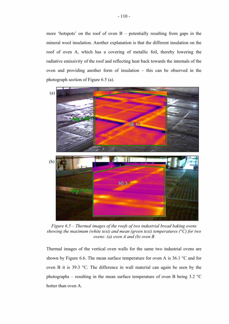
- 110 -

more ‘hotspots’ on the roof of oven B – potentially resulting from gaps in the

mineral wool insulation. Another explanation is that the different insulation on the

roof of oven A, which has a covering of metallic foil, thereby lowering the

radiative emissivity of the roof and reflecting heat back towards the internals of the

oven and providing another form of insulation – this can be observed in the

photograph section of Figure 6.5 (a).

(a)

(b)

Figure 6.5 – Thermal images of the roofs of two industrial bread baking ovens showing the maximum (white text) and mean (green text) temperatures (°C) for two

ovens: (a) oven A and (b) oven B

Thermal images of the vertical oven walls for the same two industrial ovens are

shown by Figure 6.6. The mean surface temperature for oven A is 36.1 °C and for

oven B it is 39.3 °C. The difference in wall material can again be seen by the

photographs – resulting in the mean surface temperature of oven B being 3.2 °C

hotter than oven A.

- 111 -

(a)

(b)

Figure 6.6 – Thermal images of the outer walls of two industrial ovens: (a) oven A and (b) oven B

6.6 Sensitivity Analysis of System-Level Model

As with any model aiming to approximate the behaviour of a real system, it is

essential to verify the applicability of the methodologies used in order to check the

outputs can be relied upon. For this system model of heat energy use of bread

ovens, the sensitivity of outputs is measured with respect to changes in input

variables. In this case, two separate sensitivity analyses have been conducted which

aim to quantify the consistency of the model generated.

Firstly, as shown by Figure 6.7, each input variable was changed by ± 10 % and the

resultant change on the output was recorded. The figure of 10 % was subjectively

chosen as a value within which most measurements can be performed with little

cost or specialist equipment.

It can be seen that for changes in gas metering measurements, an equivalent change

in the output is noted – therefore it is important that the gas metering values can be

relied upon. As a safety and billing accuracy measure, gas meters are annually

inspected by registered professionals to ensure the integrity of the readings. In

- 112 -

addition, a simple check is conducted by adding the sum of gas sub meters to

ensure they equal the total of the main gas supply meter (the meter that energy

supply companies use to formulate energy bills) will show any discrepancy in the

metering data.

Figure 6.7 – Sensitivity analysis showing the effect on outputs based on a 10 % change of each input variable

Other input measurements that have a significant influence on the results (over 3

%) are throughput, conveyor temperature (in and out) and final product

temperature. Of these, throughput is calculated exactly by the bakery, as all

produce and wastage is accounted for and the final product temperature as a quality

0.06%

0.16%

0.31%

0.34%

0.35%

0.44%

0.60%

0.69%

0.73%

0.81%

1.18%

1.18%

1.30%

1.42%

1.65%

1.86%

1.93%

2.02%

2.95%

2.95%

3.65%

4.06%

4.78%

6.90%

10.00%

0% 5% 10% 15%

Percentage of starch in product

Oven width

Oven height

Lid weight

Initial lid temperature

Initial tin temperature

Roof surface temperature

Final lid temperature

Conveyor mass per metre length

Bake time

Flue gas temperature

Flue gas flow rate

Oven length

Tin weight

Initial product temperature

Final tin temperature

Side wall temperature

Ambient air temperature around oven

Initial product weight

Final product weight

Final product temperature

Conveyor temperature in

Conveyor temperature out

Throughput finished product

Oven gas usage

Input variable

Total effect on output (%)

- 113 -

requirement is kept within ± 1 °C (< 1.05 %). Conveyor temperature is more

difficult to accurately measure due to the inaccessibility of the slats due to the

dangers of the chain mechanisms that drive the rotation, however the accuracy of

measurement is still well within the 10 % boundary, resulting in a potential error

accuracy of less than 5 %. Input variables that have little effect on the outputs

include the oven dimensions (width and height), the percentage of starch in the

product and the tin specifications/ temperatures. Although an increase in the oven

width would result in a larger cavity to fill with hot air, the overall throughput of

the oven would increase so a large increase in energy is not necessarily inevitable.

The effect of the increase in oven height has little effect on the energy use as it is

assumed that the volume of the baking chamber would be unaffected, therefore it is

only the wall losses that are increased.

Secondly, as shown by Figure 6.8, a compound sensitivity analysis was conducted.

This analysis considered the maximum expected degree of error for each of the

inputs – taking into account both procedural error and the accuracy of equipment

given by the OEM – usually gathered from the technical manual provided.

Figure 6.8 – Compound sensitivity analysis based on changing each input variable by the expected precision of the measurement and the instrument accuracy supplied

by the manufacturer

0%

20%

40%

60%

80%

100%

Per

cen

tage

of

hea

t as

a

pro

por

tion

of

gas

inp

ut

- 114 -

In this case, the most sensitive outputs were the flue gas losses and conveyor

losses. As experimental measurement of these two energy losses involved indirect

measurements due to the harsh environment in which bread ovens operate, scope

for error can be expected. Improvements to the measurement of conveyor

temperature could be improved by permanently soldering a thermocouple to the

conveyor slats and mounting a temperature-resistant wireless data logger to the

conveyor. This would, however, require a significant amount of downtime for a

bakery and would therefore damage the ease and applicability of the system model.

Measuring the flue gas flow rate has historically been done by use of pitot tubes, a

technique that can be less accurate than direct measurement of air velocity, as the

flow rate is inferred from pressure. Other techniques for predicting flow include

CFD modelling, acoustic velocimetry, laser anemometry or hot-wire measurement

(Jahnke, 2000). However, due to the complexities and expense of these methods

(which also rely on inference), it is doubtful that industry would adopt them for the

purpose of system modelling of bread oven energy efficiency.

6.7 Sample Results

Two commercial bread ovens at separate sites have been analysed for energy

efficiency for the purposes of this report in order to demonstrate the applicability of

the system model. Oven A was installed in c. 2009 and oven B c. 2006, with

product throughputs of 6,500 kg/hr and 9,000 kg/hr respectively. At the time of

analysis both ovens were operating at steady state producing the same product

recipe.

The specific energy consumption of ovens A and B were 804 and 920 kJ/kg

respectively. The minimum theoretical energy required to bake the bread that

comes in three forms (heat the dough, evaporate moisture and gelatinise starch) is

476 kJ/kg, which is equivalent to 59.2 % of the oven gas supply for oven A and

51.7 % for oven B, making oven A significantly more efficient. Figure 6.9 shows

- 115 -

the distribution of energy losses, illustrating the main difference is the losses

though the walls and roof, whilst the other losses are comparable. ‘Other’ losses are

the remaining heat flows deduced from Eq. (6.16) – and can be predominantly

attributed to hot air leaks from the oven. Ovens are designed with inner and outer

walls, where hot air can flow in the volume between the two. This air has a

tendency to escape from leaking joints, particularly in the roof area of the oven,

where pressure-relief panels are joined to the solid frame structure. Hot air leaks

can also occur around the access doors. Access doors and pressure-relief panels are

both regulatory requirements.

Figure 6.9 – Sample results of heat distributions obtained by system-level model for two commercial baking ovens

6.8 Opportunities for Energy Savings

Having assessed the distribution of heat loads for the oven, bakeries have looked to

analyse where energy savings can be made for financial benefit and carbon

reductions. The two focusses are on: (i) reducing the energy into the oven by

reducing the losses to ambient, and (ii) recovering heat from the oven in order to

provide energy for other processes.

0

50

100

150

200

250

300

Hea

t fl

ow (

kJ/

kg)

oven A

oven B

- 116 -

6.8.1 Oven Insulation

One outcome based on this system model was to quantify the heat losses through

the walls and roof – and it was found that the most significant heat loss from the

oven surfaces for industrial ovens was through the roof. Whilst regulatory

restrictions for pressure relief panels to be placed on the roof make it prohibitive to

have the same level of insulation as the oven walls, it was found that for new

designs of oven the insulation thickness for the whole oven could be increased by

50 mm from 150 to 200 mm for minimal additional capital cost. Further

investigation will be required to assess the efficiency gains as a result of this

improvement.

6.8.2 Conveyors

Due to the thermal mass of the conveyors, energy losses are significant. One

solution that is currently being trialled on a new generation of commercial ovens is

to have ‘enclosed terminal ends’. This solution will help to ensure that the heat

losses from the conveyor are recovered into the oven recirculation ducts. The

technology provides an extension to the hoods that already cover the entrance and

exit, and will completely eliminate the conveyor losses from the oven – though a

full regression analysis over a prolonged period would need to be conducted to

investigate whether the overall energy efficiency of the oven is improved. The

disadvantage of this technology is that the oven internal volume is larger, requiring

a greater quantity of hot air.

6.8.3 Tins and Lids

Due to the nature of square-edged loaves of bread, tins and lids are a necessary

energy load. Since they are cycled through the baking process several times per

day, they are required to be robust. Reduction to the mass or specific heat capacity

of bread tins and lids with the aim to reduce energy losses has been an interest for

bakers for many years. Although increasingly commonplace in home-baking,

silicone tins have been deemed too weak to withstand long term use in a

- 117 -

commercial bakery. Furthermore, there is a perceived risk of product contamination

from silicone coming into contact with food products. Efforts have already been

made to reduce the mass of the current design of steel tins, though for full

replacement there is a significant capital cost associated.

6.8.4 Heat Recovery

Heat recovery is an established way to reuse energy from waste heat streams for the

same or another process – historic suggestions of ways to recover waste heat in

bread baking are discussed in section 2.1.3. Heat recovery from flue gases is the

most obvious form of recuperating energy for an industrial oven. There is a large

quantity of heat being exhausted directly to atmosphere which does not require

treating. Whilst the flue gas temperature is considered ‘low grade’, at temperatures

less than 200 °C (Bending and Eden, 1984), there are still possibilities to recover

heat.

Processes that require heat in a bakery need to be identified before a heat recovery

system can be designed. One use of waste heat can be to pre-heat burner inlet air –

this is logical, as the flue is naturally located close to the burner fresh air supply.

The main challenge is to ensure the burner is suitable to run off pre-heated air,

though retrofitting or replacement of unsuitable burners can allow this. Washing

systems; both industrial pan washing machines and Clean-In-Place (CIP) require

heat and depending on the location, this can be feasible. Office and warehouse

heating demand is seasonal and weather dependent, so is not an ideal heat recovery

option. Finally, a study by the Campden & Chorleywood Food Research

Association (CCFRA) and Bristol University (2008) analysed the opportunities in

the food industry (including bread baking) to use waste heat to power Stirling

engines thereby generating electricity for the factory. This was deemed unfeasible

at the time due to insufficient technology to make the engines commercially viable.

Furthermore, as the maximum theoretical efficiency was calculated to be 40 %

- 118 -

(excluding frictional losses), the majority of heat recovered mechanically in this

way would still be wasted.

Turner (1993) warns of the dangers of exploiting waste energy from a process to

recover to a secondary process, advising the first process may suffer if the heat

streams are not managed properly. In the 1990s a large plant bakery in the UK

suffered a potentially dangerous explosion when trying to recover heat off an oven

to supply heat to the prover. This was due to mismanagement of waste heat streams

(Ward, 2010).

6.9 Temperature and Velocity Profiles in a Pilot Oven

Temperature and velocity profiling gives the local value down an oven length. In

common with section 6.8, temperature and velocity measurements in commercial

ovens are not strictly necessary for the system-level model described. However,

these measurements can result in important diagnostic data that help bakers and

oven designers to understand the effects of changes to plant equipment in their

search for energy savings.

This section presents profiles of temperature and velocity through a 9 m long pilot

oven used by oven manufacturers to trial bake profiles of new products and

experiment on new heating technologies. The oven is a scaled-down replica of an

industrial oven and is approximately 30 % the size. The significance of temperature

and velocity profiles in relation to energy is that there is an energy cost associated

with increasing the airflow necessary to achieve greater airflow uniformity.

6.9.1 Temperature Profiles

Temperature profiling is a common technique used by chain bakeries and their

oven manufacturers or installation engineers to benchmark baking characteristics in

order to maintain product consistency between different ovens or sites. The

advantage of measuring temperature, rather than other flow characteristics such as

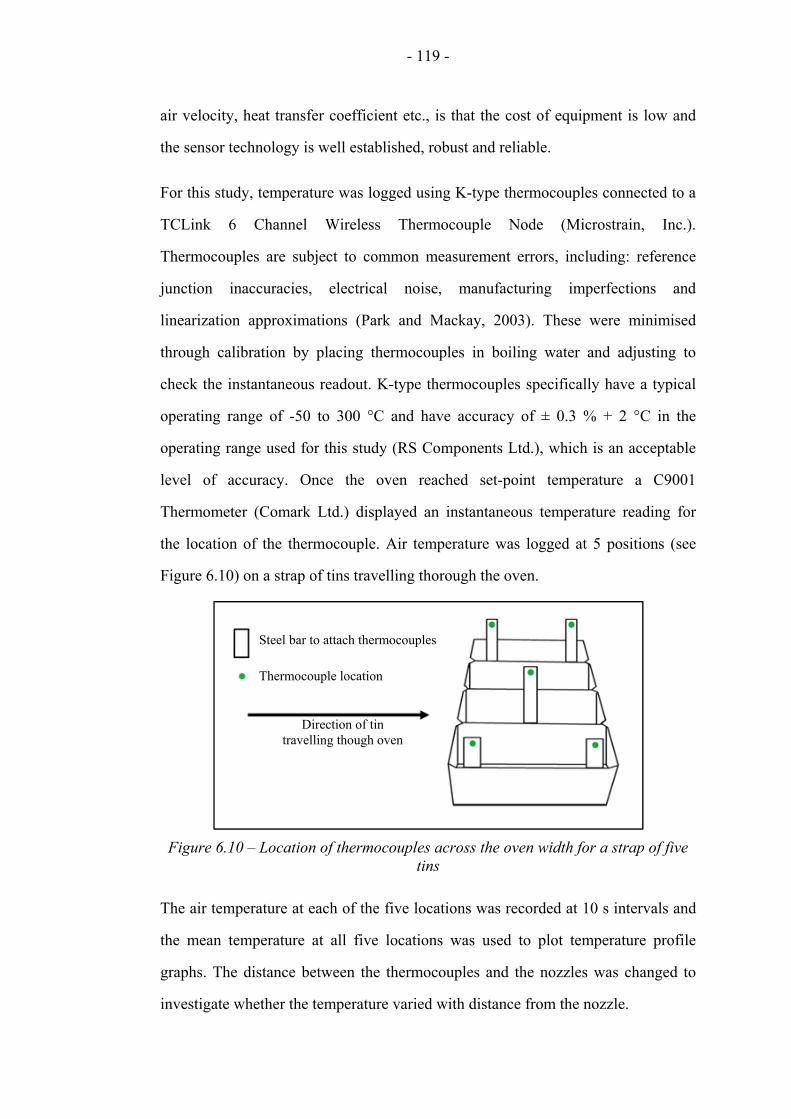
- 119 -

air velocity, heat transfer coefficient etc., is that the cost of equipment is low and

the sensor technology is well established, robust and reliable.

For this study, temperature was logged using K-type thermocouples connected to a

TCLink 6 Channel Wireless Thermocouple Node (Microstrain, Inc.).

Thermocouples are subject to common measurement errors, including: reference

junction inaccuracies, electrical noise, manufacturing imperfections and

linearization approximations (Park and Mackay, 2003). These were minimised

through calibration by placing thermocouples in boiling water and adjusting to

check the instantaneous readout. K-type thermocouples specifically have a typical

operating range of -50 to 300 °C and have accuracy of ± 0.3 % + 2 °C in the

operating range used for this study (RS Components Ltd.), which is an acceptable

level of accuracy. Once the oven reached set-point temperature a C9001

Thermometer (Comark Ltd.) displayed an instantaneous temperature reading for

the location of the thermocouple. Air temperature was logged at 5 positions (see

Figure 6.10) on a strap of tins travelling thorough the oven.

Figure 6.10 – Location of thermocouples across the oven width for a strap of five tins

The air temperature at each of the five locations was recorded at 10 s intervals and

the mean temperature at all five locations was used to plot temperature profile

graphs. The distance between the thermocouples and the nozzles was changed to

investigate whether the temperature varied with distance from the nozzle.

Steel bar to attach thermocouples

Thermocouple location

Direction of tin travelling though oven

- 120 -

Figure 6.11 shows air temperature underneath the nozzles compared with the

burner set point profile through the length of the pilot oven. The three zones are

clearly recognizable by the temperature profiles, where Tz1 = 240 °C, Tz2 = 275 °C

and Tz3 = 265 °C. Actual air temperature through the oven is consistently lower

than the burner set point. Although there is a defined shape, there are local

temperature variations, particularly further away from the nozzles. Fluctuations in

temperature are to be expected for turbulent flow, though it can be observed that

these fluctuations are localised, meaning the overall heat profile experienced by a

loaf of bread is likely to be uniform down the length of the oven. The reason for

these variations being slightly more noticeable further from the nozzle plates, i.e.

for H = 80 and 100 mm, is that there is more mixing with the surrounding air and

greater interaction with other nozzle jets. Also noticeable from Figure 6.11 is the

temperature at the entrance and exit of the oven, which is significantly below set

point temperature. This is caused by a negative pressure gradient which draws

ambient air into the oven from the ends. There is little dependence on air

temperature with relation to distance beneath the nozzles due to the strong turbulent

mixing within the oven.

Figure 6.11 – Graph of temperature profile through a pilot oven for different distances underneath the top nozzles: 20, 40, 60, 80 and 100 mm compared with

burner set point temperature (solid red line)

0

50

100

150

200

250

300

0 1 2 3 4 5 6 7 8 9

Tem

per

atu

re (

°C)

Distance along oven (m)

20mm 40mm 60mm 80mm 100mm

Zone 1 Zone 2 Zone 3

- 121 -

The statistics for the temperature distribution profiles given in Table 6.2 show the

degree of variation for each zone. As expected, the middle zone remains hotter than

227 °C for the entire oven length, whereas the temperature in zones 1 and 3, which

are exposed to the ambient air at the oven entrance and exit, drops to below 140 °C

in both cases. The mean temperature for zones 1, 2 and 3 as a proportion of the

burner set points are 88.3, 96.4 and 91.6 % respectively – consistently below the set

point temperatures. The reason for this is because the thermocouple that controls

the burner firing rate is located in the plenum above the nozzles, where the flow is

not cross-mixed with other zones or ambient air and consequently the air

temperature has not decreased.

Zone Maximum temperature (°C)

Minimum temperature (°C)

Mean temperature (°C)

Mean temperature as a proportion of set-point temperature (%)

1 234.5 105.9 211.9 88.3

2 270.6 227.0 265.0 96.4

3 266.0 130.7 242.6 91.6

Table 6.2 – Data statistics showing the variation of temperature in comparison with burner set points for each oven zone

In an energy context, temperature uniformity throughout the volume of the oven is

driven by the flow of air. For high airflow, temperature uniformity is increased due

to a high degree of mixing, whereas for low airflow the opposite is true. Increasing

air velocity has an associated energy cost which is discussed in section 6.9.2.

6.9.2 Velocity Profiles

Velocity profiles of commercial ovens are not routinely conducted on new

installations, unlike temperature profiling. Equipment for velocity measurement in

hot environments is expensive and often prohibitive due to manufacturing

schedules and the delicate nature of the baking process. Measurements are

therefore frequently made in cold ovens with recirculation and exhaust fans

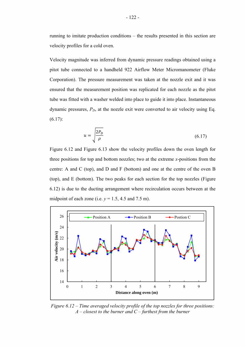
- 122 -

running to imitate production conditions – the results presented in this section are

velocity profiles for a cold oven.

Velocity magnitude was inferred from dynamic pressure readings obtained using a

pitot tube connected to a handheld 922 Airflow Meter Micromanometer (Fluke

Corporation). The pressure measurement was taken at the nozzle exit and it was

ensured that the measurement position was replicated for each nozzle as the pitot

tube was fitted with a washer welded into place to guide it into place. Instantaneous

dynamic pressures, PD, at the nozzle exit were converted to air velocity using Eq.

(6.17):

2

(6.17)

Figure 6.12 and Figure 6.13 show the velocity profiles down the oven length for

three positions for top and bottom nozzles; two at the extreme x-positions from the

centre: A and C (top), and D and F (bottom) and one at the centre of the oven B

(top), and E (bottom). The two peaks for each section for the top nozzles (Figure

6.12) is due to the ducting arrangement where recirculation occurs between at the

midpoint of each zone (i.e. y = 1.5, 4.5 and 7.5 m).

Figure 6.12 – Time averaged velocity profile of the top nozzles for three positions: A – closest to the burner and C – furthest from the burner

14

16

18

20

22

24

26

0 1 2 3 4 5 6 7 8 9

Air

vel

ocit

y (m

/s)


Position A Position B Postion C

- 123 -

Slightly more variable flow can be observed in the first and final sixth of the pilot

oven (y < 1.5 m and y > 7.5 m), which can be attributed to the increase in mixing

between the jets and the ambient air. The decrease in air velocity in the same

regions for the bottom nozzles (Figure 6.13) is another feature of the design of the

pilot oven – the plenum below the bottom nozzles is designed with ducting located

nearer to the oven centre, which reduces the quantity of air escaping from the oven

entrance and exit.

Figure 6.13 – Time averaged velocity profile of the bottom nozzles for three positions: D – closest to the burner and F – furthest from the burner

Figure 6.14 and Figure 6.15 show three-dimensional plots of velocity distribution

for top and bottom nozzles respectively. Figure 6.14 further illustrates the non-

uniformity of velocity across the width for the top nozzles – where the velocity at

the centre of the oven is consistently greater than that at the outer edges.

Conversely, Figure 6.15 illustrates the large degree of uniformity across the width

of the oven for the bottom nozzles, which occurs due to the plenum design. The

uniformity of the velocity profiles can be expressed in terms of deviation from the

centre nozzle velocity; for the top nozzles: -9 % < uB < 11 % and for the bottom

nozzles -6 % < uE < 2 %.

14

16

18

20

22

24

26

0 1 2 3 4 5 6 7 8 9

Air

vel

ocit

y (m

/s)


Position D Position E Position F

- 124 -

Figure 6.14 – Three-dimensional profile of velocity through a pilot oven for top nozzles: A – closest to the burner and C – furthest from the burner

Figure 6.15 – Three-dimensional profile of velocity through a pilot oven for bottom nozzles: D – closest to the burner and F – furthest from the burner

In order to increase the velocity uniformity of impingement jets, a more uniform

pressure drop across the nozzle bank is necessary. The way this is usually

controlled is by increasing the static pressure in the plenum above the nozzle

orifices. The additional energy cost associated with this pressure increase is

01.5

34.5

67.5

9

16

18

20

22

24

26

A B C

24-26

22-24

20-22

18-20

16-18

01.5

34.5

67.5

9

16

18

20

22

24

26

D E F

24-26

22-24

20-22

18-20

16-18

Air

vel

ocit

y (m

/s)

Air

vel

ocit

y (m

/s)

- 125 -

dictated by the electricity load required to operate the recirculation fans at a higher

speed. The balance between the additional electricity load required for increased air

distribution and the heat savings made possible as a result of a faster bake time are

discussed further in Chapter 7.

6.10 Summary

The system-level thermodynamic analysis methodology presented here has been

used to assess the energy performance of bread ovens. This is a rigorous scientific

framework that has been developed via systematic research and has been widely

used by bread manufacturers to measure, predict and reduce the energy demand of

current ovens. Furthermore, oven designers have used the findings to influence the

future design of the next generation of ovens. This work has been combined with a

CFD optimisation to estimate annual savings of over £0.5 million and 5,000 TCO2e

for the UK (Paton et al., 2011, Paton et al., 2012b).

The use of thermal imaging to help determine surface temperature and thus

calculate heat losses from the oven walls provides a new, non-invasive approach to

quantify convective losses to atmosphere. Temperature and velocity profiles on a

pilot oven provide an example of measurement techniques that can be used to

pragmatically benchmark bread oven heat and airflow characteristics. Temperature

and velocity uniformity are not only important quality constraints that dictate the

consistency of products, but are also factors that have an impact on energy use of

bread ovens, due to the increase in fan power required increase air distribution and

the pressure drop across the plenum. The energy cost of this is investigated further

in Chapter 7.

A sensitivity analysis indicates the equations and methodologies used in the model

are suitable, provided appropriately accurate instrumentation is used and careful

experimental procedures are executed. The sample results show the validity of the

model, and give an idea of the scale of the energy demand of bread ovens. The

- 126 -

widely reported figure that half the heat in a bread oven is wasted has been

corroborated to an extent and uniquely, the losses to ambient have been quantified

and incorporated into a flexible model that has been extensively used in industry.

- 127 -

Chapter 7

Experimental Measurements of Local and

Global Heat Transfer Characteristics

In the previous chapter, the methodology for a system-level thermodynamic

analysis of industrial bread baking ovens was outlined. In addition to this,

experimentation on the heat transfer characteristics inside commercial ovens is

necessary to gain an appreciation of how airflow can affect product quality and

energy efficiency. Experimental results allow equipment designers to develop

ovens with optimum heat transfer rates. Optimum heat transfer means an

improvement in energy efficiency whilst maintaining the essential product

characteristics required by bakeries.

This chapter describes experimental methods and presents novel results that are

intended to be used by oven designers and bakery operators to influence both oven

design and operating conditions to increase energy efficiency of commercial baking

ovens. The aim of this chapter is to measure the radiative and convective heat

transfer coefficient for jet impingement nozzle designs relevant to bread baking

ovens. The heat transfer coefficient is directly linked to factors such as jet velocity

and nozzle-to-surface distance – these relationships can be converted into an cost to

determine an optimum heat transfer coefficient, which can then be translated into a

set of operating conditions for an oven.

7.1 Background

According to Ovadia and Walker (1998) there are at least nine different ways to

heat food; the three conventional methods outlined in section 3.1: conduction,

convection and radiation, and four further modes: microwave, capacitive heating,

electrical resistance heating and intense visible light. In general (and studied here),

the bread baking process uses hot air to transfer heat to the dough surface through

convection. Thermal radiation is also used to transfer heat between the internal

- 128 -

oven surfaces and the bread. Heat is then transferred to the centre of the dough via

conduction.

Relatively high rates of heat transfer can be achieved with comparatively low air

temperatures through jet impingement heat transfer, which is discussed in detail in

section 3.2. Although jet impingement heat transfer is a well understood

phenomenon, little work has been published relating to local heat transfer

characteristics specific to bread-baking regimes. As discussed in section 3.2, much

of the previously published work on jet impingement heat transfer has focussed on

generating correlations for ASME standard nozzles. Whereas in practice, baking

ovens are designed in the most cost-effective manner, meaning the nozzles are, in

reality, sharp-edged punched holes in sheets of metal. These sheets are attached to

pressure plenums above and below the product surface. Due to this, the heat

transfer characteristics of jet impingement nozzles in industrial applications can

differ somewhat to those reported in literature.

7.2 Experimental Apparatus

In order to measure mean and local heat transfer rates in the regimes relevant to the

baking industry, experiments on a scaled down baking oven were carried out. The

pilot oven, named the ‘hand sampling machine’, located at Spooner Industries Ltd.,

Ilkley, was designed to carry out small scale experiments using jet impingement for

the food, coating, paper, thin-film, and other drying industries. One of the main

advantages of being able to use this specialised drying apparatus was the ability to

reproduce a wide range of conditions that are relevant to bread baking. This

included the use of different nozzle designs, air velocities and dimensions of

important geometries such as nozzle-to-surface distance.

Improvements in heat flux measurement technology over the past two decades have

meant commercial sensors are now available that can measure and log heat transfer

rates locally underneath nozzle orifices. The experimentation discussed in this

- 129 -

section makes use of these sensors to give correlations and results that are useful to

oven designers and operators when assessing heat transfer in commercial ovens.

7.2.1 The Pilot Oven

A photograph of the oven used for the heat transfer experimentation is shown in

Figure 7.1:

Figure 7.1 – Partially labelled photograph of the pilot oven used for heat transfer experiments

A labelled schematic of the pilot oven is shown by Figure 7.2, and the features are

explained in Table 7.1. The overall dimensions of the oven were 2.5 m (height) x 4

m (width) x 4 m (length). 100 mm thick insulation panels cover each face of the

machine, ①. Banks of nozzles were attached to the baking chamber above and/ or

below the sensor position by sliding plates into mounting slots and bolting into

place, ② and ③. Heat was supplied from a natural gas burner (Comtherm Limited)

(up to 500 kW), which was further insulated for health and safety reasons, ④. K-

type thermocouples located inside the oven plenum chamber fed into a PID

controller which maintained consistent nozzle jet temperatures of up to 400 °C. The

oven could reach steady set-point temperature within 30 minutes.

Combustion air was circulated to the top and bottom nozzle banks via a centrifugal

recirculation fan which used a VSD to control air velocity, ⑤. This system allowed

Burner

Oscillating arm

Recirculation fan

- 130 -

nozzle exit velocities of between 10 and 60 m/s to be achieved. Manual dampers

were located in the ducting between the recirculation fan and the nozzles which

gave further control of air velocity to top and bottom nozzle banks, ⑥ and ⑦. For

this study, only the top set of nozzles were used to give heat transfer rates of one

set of impingement jets. An exhaust duct was located above the oven, which

removed a proportion of the air to atmosphere to expel the products of combustion.

The remainder of the air was recirculated in order to maintain oven temperature

and airflow, ⑧. An integrated centrifugal exhaust fan was located in the exhaust

duct, ⑨. The proportion of recirculated/ exhausted air was controlled by a manual

air damper, ⑩.

A heat flux sensor was used to measure and log the heat transfer characteristics

created by the oven conditions, ⑪. The sensor was reciprocated below the top

nozzle set by a specialised rig which used a motor, gearbox and extension arm to

oscillate the sensor at a set frequency and displacement range, ⑫.

Figure 7.2 – Schematic of the pilot oven used for heat transfer experiments

- 131 -

# Equipment Description

①

Outer insulation: 100 mm thick outer insulation panels were used to maintain oven temperature and keep the operation of the pilot oven safe.

② Top nozzle plate: Different nozzle banks could be attached to supply airflow above the product.

③ Bottom nozzle plate:

Different nozzle banks could be attached to supply airflow below the product.

④ Burner: Natural gas was supplied to the burner and combustion air was regulated to maintain a constant quantity of excess air (typical AFR ~ 2).

⑤ Recirculation fan and ducting:

A 22 kW fan was used to distribute air to the top and bottom nozzle plenums.

⑥ Top nozzle recirculation dampers:

Manual dampers were used to control the flow rate of air to the top nozzle banks, and thus jet velocity.

⑦ Bottom nozzle recirculation dampers:

Manual dampers were used to control the flow rate of air to the bottom nozzle banks, and thus jet velocity.

⑧ Exhaust duct: Hot flue gases were exhausted to a centralised duct to be safely released to atmosphere.

⑨ Exhaust fan: A 7.5 kW fan was used to expel exhaust air and maintain the oven at negative pressure. This ensured there were no hot air leaks out of the oven entrance.

⑩ Exhaust damper: A manual damper was adjusted to determine the ratio of air that was recirculated and air that was exhausted to atmosphere.

⑪ Heat flux sensor: Commercially available sensor used to measure local heat flux profiles and deduce values for heat transfer coefficient.

⑫ Reciprocating arm: A motor and gearbox connected to a VSD allowed the sensor to be oscillated at a set velocity and traverse range. An arm was attached to the gearbox drive chain at one end and the heat flux sensor at the other.

Table 7.1 – Description of features of pilot oven

7.2.2 Nozzle Types

Two nozzle sets were used for comparison, an array of slot nozzles (ASN),

consisting of rows of thin slots (or slits) and an array of round nozzles (ARN),

consisting of rows of round holes. Both sets of nozzles were formed from 1.8 mm

thick mild steel sheets.

- 132 -

The ASN arrangement, shown by Figure 7.3, consisted of a long array of 5 mm

slots (more than 10 rows) pitched 230 mm apart in the x-direction. To maintain the

slot width the folded metal sheets were welded together at a 5 mm gap at 200 mm

intervals in the z-direction. ASNs are typically used for drying of food, paper,

plastic film or metallic sheets (Wimberger, 1999). The reason for selecting this

arrangement is that a number of correlations for heat transfer already existed for

ASNs, meaning experimental results can be compared with the correlations

reported in literature.

Figure 7.3 – ASN arrangement for heat transfer experiments

The ARN arrangement, shown by Figure 7.4, consisted of 36 x 12 mm diameter

round holes spaced 22 mm apart across the width (z-direction), and pitched 230

mm along the length of the oven (x-direction). The ARN arrangement used is

typical of those used in bread baking and differs from many studies reported in

literature as the distance between the holes were asymmetrically distributed (i.e. the

distance between holes down the length of the oven, x-direction, 230 mm, was

more than ten times the distance across the width of the oven, z-direction, 22 mm).

The holes for this nozzle arrangement were made using a CNC (computer

numerical control) laser cutting machine.

Figure 7.4 – ARN arrangement for heat transfer experiments

5 mm

180 mm 50 mm

121.5 °

230 mm 22 mm ϕ 12 mm

- 133 -

For the ARN, relative nozzle area, f, was calculated using Eq. (7.1), which has been

altered to incorporate the asymmetry of the nozzle set used:

4 ∙

(7.1)

The relative nozzle area for the ASN was calculated by Eq. (7.2):

(7.2)

The specifications for the two types of nozzle under investigation are shown by

Table 7.2:

Nozzle type ASN ARN

Nozzle diameter/ width, d (mm) 5 12

Characteristic length, Lc (mm) 10 (= 2d) 12 (= d)

Nozzle pitch, P (mm) 230 200

Ratio of pitch to diameter, P/d 46.00 16.67

Hole spacing, S (mm) n/a 22

Relative nozzle area, f 2.174 % 2.235 %

Table 7.2 – Dimensions and specifications for the nozzle configurations investigated

7.2.3 The Heat Transfer Sensor

The heat transfer sensor used in this study is a commercially available RC01 heat

flux sensor (Hukseflux Thermal Sensors, c. 2010), see Figure 7.5:

Figure 7.5 – Photograph of Hukseflux RC01 heat flux sensor (Hukseflux Thermal Sensors, c. 2010)

①

②

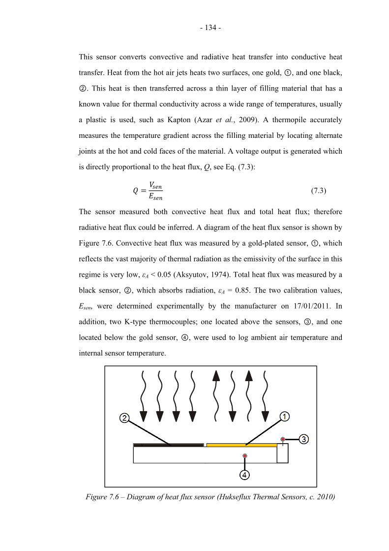
- 134 -

This sensor converts convective and radiative heat transfer into conductive heat

transfer. Heat from the hot air jets heats two surfaces, one gold, ①, and one black,

②. This heat is then transferred across a thin layer of filling material that has a

known value for thermal conductivity across a wide range of temperatures, usually

a plastic is used, such as Kapton (Azar et al., 2009). A thermopile accurately

measures the temperature gradient across the filling material by locating alternate

joints at the hot and cold faces of the material. A voltage output is generated which

is directly proportional to the heat flux, Q, see Eq. (7.3):

(7.3)

The sensor measured both convective heat flux and total heat flux; therefore

radiative heat flux could be inferred. A diagram of the heat flux sensor is shown by

Figure 7.6. Convective heat flux was measured by a gold-plated sensor, ①, which

reflects the vast majority of thermal radiation as the emissivity of the surface in this

regime is very low, εA < 0.05 (Aksyutov, 1974). Total heat flux was measured by a

black sensor, ②, which absorbs radiation, εA = 0.85. The two calibration values,

Esen, were determined experimentally by the manufacturer on 17/01/2011. In

addition, two K-type thermocouples; one located above the sensors, ③, and one

located below the gold sensor, ④, were used to log ambient air temperature and

internal sensor temperature.

Figure 7.6 – Diagram of heat flux sensor (Hukseflux Thermal Sensors, c. 2010)

- 135 -

The sensor was mounted onto a nickel heat sink to ensure high thermal

conductivity away from the filling material to prevent both surfaces reaching

thermal equilibrium. Underneath the heat sink was a water-cooled block which

dissipated heat away from the system.

The maximum temperature for measurement for this type of sensor is 250 °C, and

the maximum flux that the sensor could be exposed to was experimentally

determined for each particular regime. The accuracy of the heat flux sensor was

given by the manufacturer as ± 10 % for total heat flux.

The sensor was connected to a TL01 Heavy Duty Data Logger (Hukseflux, The

Netherlands), which logged results at 2 second intervals from four separate

channels: ambient air temperature, ①, internal sensor temperature, ②, heat flux at

black plate, ③ and heat flux at gold plate, ④ (see Figure 7.6). The logger could

store up to 47,662 readings (equivalent of 26 hours of data), which was sufficient

for this study. Live readings and the status of the sensor could be viewed via

specialised ‘TL01 Ovenlogger Application’ software connected via USB to a PC.

Heat transfer sensors and the accuracy of their readings are discussed in detail by

other authors: (Childs et al., 1999, Diller, 1993). For the purposes of this report, the

heat transfer results are compared with literature to validate their accuracy.

7.3 Methodology

In order to conduct heat transfer experiments the conditions within the oven had to

be carefully prepared. The exhaust fan on the pilot oven was turned on to ensure

any unburned gas was expelled from the oven before the burners were ignited. This

was done with all dampers fully open and the recirculation fan running to circulate

air throughout the ducts and oven plenum chambers. Once the purge cycle was

complete, the burners were ignited. Hot air and combustion products were

recirculated until set temperature was reached. The oven was then left for

approximately 30 minutes for the internal temperature to stabilise.

- 136 -

Nozzle exit velocity was calculated from two temperature corrected static pressure

readings from the oven plenum. The first reading was from a mounted pressure

gauge which was connected directly to the plenum chamber above the top nozzles.

The second reading was taken from a P200UL Digital Manometer (Digitron

Instrumentation Limited, UK) attached to a tapping point connected directly to the

top nozzles. Mounted pressure gauges and tapping points were also located at the

bottom nozzle plenum chamber. The velocity values inferred were corroborated by

pitot tube measurements taken at the nozzle exit. The accuracy of the manometer

measurements is given in the P200UL manual as ± 0.1 % FS + 1 digit, i.e. 0.02

mbar. Measurements were between 0.13 and 2.00 mbar, giving potential percentage

error in nozzle jet air velocity readings, unoz, of between 1.00 and 15.38 %.

The heat flux sensor was housed in a square-shaped aluminium holding rig, with

dimensions of 0.5 m x 0.5 m, made out of 1.8 mm thick aluminium sheet. This

ensured the sensor was flush to the surface of the aluminium rig, thus not affecting

the airflow field around the sensor. An adjustable bracket on the back of the sheet

fixed the sensor in place. This rig was fixed to a steel frame which prevented the

rig from bending under the high-velocity air jets and maintained consistent nozzle-

to-surface distances, H.

The sensor and holding rig were reciprocated in the x-direction (the length of the

oven) via a gearbox and motor configuration housed outside the pilot oven

entrance. The velocity of the reciprocator could be altered using a VSD which

controlled the motor speed. The minimum velocity of the reciprocating arm was 0.1

mm/s and maximum velocity was 40 mm/s. For this study, a velocity of 0.25 mm/s

was chosen, which gave a good balance of measurement profile resolution whilst

being able to conduct a complete traverse of a standard nozzle arrangement (230

mm pitch with a safety margin of at least 50 mm either side) in less than 30

minutes. Taking into account the time required to set up the equipment and to

adjust the rig between experiments, around six to eight experiments could be

- 137 -

conducted per day, which allowed time for the quantity of results presented here to

be collected.

In order for the sensor to remain functional during the tests, water cooling to the

bottom surface of the sensor was necessary. Tests were conducted to show that the

effect of using different water flow rates did not affect the results. Mains water was

supplied, and warm cooling water (around 30 °C) was discharged to drain, via two

5 m long, 5 mm inner diameter high-temperature flexible hoses. The volumetric

flow rate of cooling water through the sensor was nominally 1 x 10-5 m3/s.

When the heat flux sensor entered the pilot oven, it was left for approximately 5

minutes to allow output readings to stabilise. The sensor traversed across more than

one full nozzle pitch length in all cases. One nozzle pitch length, P, is shown

diagrammatically by Figure 7.7:

Figure 7.7 – Diagram showing minimum traverse range (P) of heat flux sensor

7.4 Validation of Experiments

An important part of this project was to validate the results of the sensor in terms of

repeatability, symmetry about a nozzle orifice and correlation of results with those

reported in literature. These issues are addressed in the following sections 7.4.1 to

7.4.3.

7.4.1 Repeatability

In order to investigate the repeatability of the experiments, the sensor was traversed

across the width of more than two complete pitch lengths of 5 mm slot nozzles (i.e.

centre-to-centre of three nozzle sets). The conditions for the repeatability study

P

- 138 -

were: Temperature, T = 200 °C, Reynolds number, Re = 4,541 and ratio of nozzle-

to-surface distance over nozzle diameter, H/d = 6. The heat flux profile

measurements for both convective and radiative heat fluxes have been shown to be

repeatable by Figure 7.8:

Figure 7.8 – Heat transfer graph indicating the degree of repeatability of the heat flux profile measurements

It is standard practice in the field of jet impingement heat transfer to display results

in dimensionless form, therefore the following results are given using this format,

meaning hc and unoz are expressed as Nu and Re respectively.

The Nusselt number profiles of the three nozzles traversed for Figure 7.8 are shown

overlaid on each other in Figure 7.9, where x/d is the dimensionless distance from

the nozzle centre. Again, it can be seen that in the region -13 < x/d < 13 the

measurements are very similar, however in the regions x/d > 13 and x/d < -13 the

Nusselt number profiles of the three nozzle sets are unsteady. This is because in

this region the flow is interacting with the adjacent jets. Jet interaction can give

unpredictable results depending on the internal ducting and fan arrangements in the

pilot oven. It is important to note that the correlation between the three nozzle

peaks is extremely high; the Pearson product-moment correlation coefficient

0

5

10

15

20

25

0 200 400 600 800 1000 1200 1400

Hea

t fl

ux

(kW

/m2 )

Sample number

Total heat flux Convective heat flux Radiative heat flux

- 139 -

(Pearson’s r value) is between 0.972 and 0.991 for the three data sets. The mean

Nusselt number values in the region -18 < x/d < 18 (the only region where all three

data sets could be equally compared) were 16.46, 17.12 and 16.72 for nozzles sets

1, 2 and 3 respectively. These values are all within 4 % error margin of each other

indicating a high degree of repeatability.

Figure 7.9 – Dimensionless heat transfer coefficient of three nozzle profiles overlaid on each other showing the degree of repeatability of the heat flux sensor

7.4.2 Heat Flux Symmetry about Nozzle Centre

The Nusselt number profiles presented in this chapter can be slightly asymmetric

due to local flux fluctuations, particularly in the region between two sets of nozzles

where external factors such as jet interaction, ducting arrangements and exhaust fan

positioning can have a greater effect on heat transfer. In small scale experiments,

these effects can be minimised by locating fans at the optimum position, however it

is important to gather an appreciation of these effects for industrial applications

using the pilot oven arrangement discussed here.

For the nozzles studied in Figure 7.8 and Figure 7.9, the asymmetry of heat flux of

nozzles 1, 2 and 3 in the region -18 < x/d < 18 is 6.54, 15.27 and 5.96 %

respectively. This level of asymmetry is typical for heat transfer measurements of

0

5

10

15

20

25

30

35

40

-25 -20 -15 -10 -5 0 5 10 15 20 25

Nu

ssel

t n

um

ber

x/d

Nozzle 1 Nozzle 2 Nozzle 3

- 140 -

arrays of jets due to the effect of interaction between jets (Geers et al., 2004). The

values of Nu for x/d > 0 and x/d < 0 are shown graphically by Figure 7.10. It can be

seen that in general slightly higher values are typically obtained for x/d > 0 than

those obtained for x/d < 0.

Figure 7.10 – Graph showing the degree of symmetry of heat flux measurements about the nozzle centre

7.4.3 Nusselt Number Correlations Compared with Literature

The effect of air velocity (Reynolds number) on mean heat transfer coefficient

(mean Nusselt number) was investigated for ASN and ARN for the set of

conditions outlined in Table 7.3. The purpose of measuring these values was to

compare the results with literature.

Nozzle type ASN ARN

Jet temperature, T, (°C) 184 to 204 192 to 200

Nozzle-to-surface distance, H (mm) 25 25

Ratio of nozzle-to-surface distance over diameter, H/d 5.000 2.083

Reynolds number, Re 3,221 to 10,902

3,711 to 13,129

Table 7.3 – Range of conditions for correlations between Reynolds number and Nusselt number

0

5

10

15

20

25

30

0 5 10 15 20 25 30

Nu

ssel

t n

um

ber

at

x/d

< 0

Nusselt number at x/d > 0

Nozzle 1

Nozzle 2

Nozzle 3

- 141 -

Heat transfer correlations for ASNs are widely available. Since their profile is

constant across the width of the oven they can be considered two-dimensional. In

addition, the nozzle profiles can be easily and consistently manufactured from sheet

metal making experimental measurements on different facilities comparable.

Experimental values for mean Nusselt number, shown in Figure 7.11, match

closely with the correlations in literature (Das et al., 1985, Hardisty and Can, 1983,

Martin, 1977). The results particularly corresponded with Das et al. (1985),

comparison with this data shows their correlation over predicted Nusselt number by

a mean percentage error of 6.7 % and a maximum percentage error of 10.2 %, and

Martin (1977), who under predicted Nu by a mean percentage error of 8.8 % and a

maximum percentage error of 13.4 %. The correlation of Hardisty and Can (1983)

was less applicable; it over predicted the Nusselt number by a mean of 30.2 % and

a maximum of 40.7 %. The wide range of correlations highlights the need for

experimental correlations to be made for the specific nozzle types under

investigation.

Figure 7.11 – Graph of Reynolds number against mean Nusselt number for ASN experimental results and correlations reported in literature

0

10

20

30

40

50

60

0 2,000 4,000 6,000 8,000 10,000 12,000 14,000 16,000

Nu

ssel

t n

um

ber

Reynolds number

Experimental results

Martin (1977) ASN

Das et al. (1985)

Hardisty and Can (1983)

- 142 -

For the ARN used, there are no correlations in literature which capture the

asymmetric nature of the hole distribution. For this reason, the results were

compared with two of the Martin (1977) correlations; ARN and ASN. This was to

test the assumption within industry that rows of closely spaced rows of round

nozzles approximate ASNs. Table 7.4 shows the alterations to the dimensions that

were necessary to approximate the correlation for ARNs as ASNs:

Nozzle type ARN ARN as ASN

Nozzle diameter/ width, d (mm) 12 5.141

Characteristic length, Lc (mm) 12 (= d) 10.282 (= 2 d)

Ratio of nozzle-to-surface distance over diameter, H/d 2.083 4.863

Relative nozzle area, f 2.235 % 2.235 %

Table 7.4 – Changes to dimensions for correlating the asymmetric ARN as an ASN

Figure 7.12 shows that the non-symmetrical ARN behaves closer to the Martin

(1977) ASN correlation than it does to the ARN correlation, particularly at lower

Reynolds numbers (Re < 10,000). The mean difference between experimental

results and the ASN correlation is 9.0 % and the maximum difference is 13.5 %,

whilst the mean difference when compared to the ARN correlations is 28.3 % and

the maximum difference is 33.2 %.

Figure 7.12 – Graph of Reynolds number against mean Nusselt number for ARN experimental results and correlations reported in literature

0

10

20

30

40

50

60

0 2,000 4,000 6,000 8,000 10,000 12,000 14,000 16,000

Nu

ssel

t n

um

ber

Reynolds number


Martin (1977) ARN

Martin (1977) ASN

- 143 -

7.5 Mean Heat Transfer Measurements

Mean heat transfer correlations are useful to industry as they give an overall value

to benchmark differences between heat transfer characteristics for a range of nozzle

configurations.

7.5.1 Correlation of Nusselt Number with Reynolds Number

The results showing how the rate of heat transfer varies with air velocity (Re versus

Nu) are shown in the previous section by Figure 7.11 and Figure 7.12. These results

are reproduced below in Figure 7.13, with a correlation that represents a good fit

when compared to both aforementioned data sets. For simplicity, the correlation to

predict the Nusselt number from the Reynolds number is given by the power

relation:

(7.4)

where, for the set of conditions used, m = 0.047 and n = 0.7.

Figure 7.13 – Graph showing Nusselt number correlations for ASN and ARN

The Coefficient of Determination (R2) value for these two sets of data when

compared to Eq. (7.4) is shown by the regression plot, Figure 7.14. R2 values of

0.9838 and 0.9928 for ARN and ASN respectively show the very high degree of

0

10

20

30

40

50

60

0 2,000 4,000 6,000 8,000 10,000 12,000 14,000 16,000

Nu

ssel

t n

um

ber

Reynolds number

ASNARNCorrelation

- 144 -

validity of the proposed correlation of Reynolds number and Nusselt number. The

correlation developed is valid for the following range of conditions, which are

relevant to bread baking applications:

3,200 < Re < 13,200

H/d = 5, d = 5 mm, f = 2.17 % for ASN

H/d = 2.083, d = 12 mm, f = 2.24 % for ARN

T = 200 °C

Figure 7.14 – Regression plot to measure R2 value of data sets compared with correlation

The correlation presented, predicts the Nusselt number as a function of Reynolds

number. This enables commercial oven designers to balance the energy flows in a

new design of oven. Heat transfer rates at greater air jet velocities will inevitably

increase production rates and therefore reduce the gas consumption of the oven.

However, this should be balanced against the additional electrical energy required

for air distribution and product quality concerns, as discussed further in section 7.7.

7.5.2 Variation of Heat Transfer with Nozzle-to-Surface Distance

It has been widely reported that maximum heat transfer rates are achieved when

H/d is between 2 and 8 (Mujumdar, 2007, Stephan, 1993), and that heat transfer

R² = 0.9838

R² = 0.9928

0

5

10

15

20

25

30

35

40

0 5 10 15 20 25 30 35 40

Pre

dic

ted

Nu

ssel

t n

um

ber

Experimentally determined Nusselt number

ASN

ARN

- 145 -

rates can be increased by 20 % by optimising H/d (Zuckerman and Lior, 2006).

Figure 7.15 shows the Martin (1977) correlations for Nusselt number compared

with H/d for Re = 5,000. The correlations show that for both ASN and ARN, heat

transfer decreases when H/d > 2.

Figure 7.15 – Martin (1977) correlations for dimensionless nozzle-to-surface distance (H/d) against Nusselt number for ASN and ARN

Experimental results of Nusselt number using the ARN for 1.33 < H/d < 7.83 are

shown by Figure 7.16. It can be seen again that these results align well with

correlations from literature, in this case Martin (1977) ASN. The degree of

accuracy of the approximation of the asymmetric ARN as ASN can be observed for

a range of H/d ratios. The experimental results have a mean percentage difference

in comparison with literature of 2.06 % and a maximum difference of 6.99 %. The

trend of slightly decreasing Nusselt number with increasing H/d is observed. This

trend is relevant to bread baking as decreasing the nozzle-to-surface distance would

be desirable to achieve higher heat transfer rates whilst maintaining the same

nozzle velocity, indicating the opportunity to decrease the baking time whilst using

the same amount of energy. Decreasing the nozzle-to-surface distance presents a

number of practical problems for bread baking; as the nozzles are closer to the

conveyor, cleaning can be made more difficult and blockages in the oven can

0

5

10

15

20

25

30

0 2 4 6 8 10 12 14

Nu

ssel

t n

um

ber

H/d

Martin (1977) ASN

Martin (1977) ARN

- 146 -

become more frequent when two dough-pieces are accidentally stacked above one

another. In order to manufacture ovens with optimum H/d ratios, these issues

require addressing.

Figure 7.16 – Comparison of experimental mean Nusselt number results for ARN at varying H/d ratio with Martin (1977) ASN correlations

7.5.3 Mean Proportion of Radiation and Convection

The quality parameters of bread are partially determined by the balance of heat

transfer to the surface of the bread through radiation and convection in the oven

(Williamson and Wilson, 2009). For a bakery chain with multiple ovens it is

important to ensure that each oven produces the same product. This can be

standardised by profiling the percentage of radiation and convection for different

operating regimes. It is known that baking cookies with a higher proportion of

radiative heat transfer results in a darker coloured product (Shibukawa et al., 1989),

and it is believed, though it is not reported in literature, that the same phenomena

applies to bread baking (Kirk, 2011). Other quality factors that are thought to be

determined by the degree of radiation include taste and density.

As the Reynolds number increases, the proportion of heat transfer due to

convection increases and radiation decreases, as shown by Figure 7.17 and Figure

0

5

10

15

20

25

30

0 1 2 3 4 5 6 7 8 9 10

Nu

ssel

t n

um

ber

H/d


Martin (1977) ASN corellation

- 147 -

7.18, for ASN and ARN respectively. This is consistent with theory, as values of

radiative heat transfer are unaffected by air velocity, whereas the convective heat

transfer increases, therefore the relative proportion convection increases and

radiation decreases.

For both sets of nozzles, the proportion of radiation decreased linearly with

increasing Reynolds number. Both graphs exhibit a strong trend, with R2 values of

0.998 and 0.978 for ASN and ARN respectively.

The linear trend line equations given for ASN and ARN give y-intercept values as

11.428 and 10.271 % respectively. This implies that for regimes with very low

airflow (Re < 500), only 10 to 12 % of heat transfer would be due to radiation – this

seems unlikely. The proportion of heat transfer due to radiation for low Reynolds

numbers would require validation, therefore the linear trends in Figure 7.17 and

Figure 7.18 can only be valid for the set of conditions that have been tested in this

study, the same as those in Table 7.3. The gradient of both trend lines is roughly

equal, further indicating that closely spaced rows of round holes can be

approximated as ASN.

Figure 7.17 – Graph of Reynolds number against mean percentage of heat transfer due to radiation for ASN

y = -0.0006x + 11.428R² = 0.998

0

2

4

6

8

10

12

14

0 2,000 4,000 6,000 8,000 10,000 12,000 14,000 16,000

Per

cen

tage

of

hea

t tr

ansf

er

du

e to

rad

iati

on (

%)

Reynolds number

- 148 -

Figure 7.18 – Graph of Reynolds number against mean percentage of heat transfer due to radiation for ARN

7.6 Local Heat Transfer Measurements

Local heat transfer measurements show the locations of maximum and minimum

heat transfer rates and detailed profiles of heat transfer across the nozzle pitch can

be observed. Local heat transfer profiles are particularly useful for oven designers

to assess the difference between maxima and minima, thus indicating the degree of

non-uniformity of the bake profile. For nozzles that are close together, or where

H/d is small, interactions between flow fields can be identified, these can have

positive or negative effects on local and mean heat transfer rates.

As the heat flux profiles have been shown to be greater than 90 % symmetric about

then nozzle centre, standard practice is followed for displaying local jet

impingement heat transfer results and the local profiles are shown for half of the

nozzle pitch (i.e. Nu only displayed for x/d ≥ 0).

7.6.1 Local Profiles of Nusselt Number with Reynolds Number

Figure 7.19 shows local dimensionless heat transfer coefficient distribution across

the ASN configuration for Reynolds numbers in the range of 3,221 ≤ Re ≤ 10,902,

for H/d = 5 and T = 200 °C. There is one primary peak at x/d = 0. Either side of this

y = -0.0006x + 10.271R² = 0.9779

0

2

4

6

8

10

12

14

0 2,000 4,000 6,000 8,000 10,000 12,000 14,000 16,000

Per

cen

tage

of

hea

t tr

ansf

er

du

e to

rad

iati

on (

%)

Reynolds number

- 149 -

peak the Nusselt number decays exponentially until the middle point of two nozzle

banks (x/d = ± 23), where the minimum value is reached. Subtle secondary peaks in

Nusselt number can be identified at x/d ≈ ± 14, indicating a small amount of

turbulence in the wall jet region; the insignificance of these peaks can be attributed

to the H/d value (5), which is around the upper limit at which secondary peaks

occur (Colucci and Viskanta, 1996).

Figure 7.19 – Graph of local Nusselt number against dimensionless distance from the centre of the nozzle jet (x/d) for ASN for five different Reynolds numbers

between 3,221 and 10,902

The H/d ratio has a dominant effect on the occurrence of secondary peaks, as they

only appear for low values (H/d < 5) (O'Donovan and Murray, 2007). This is due to

a thinning effect of confining the airflow which causes a change from transitional

to turbulent flow in the wall jet boundary layer. This increase in turbulence causes

a peak in heat transfer (Fitzgerald and Garimella, 1998). The effect of air velocity

on the appearance of secondary peaks is also well documented in literature – and is

due to the illusion that higher Reynolds number has on reducing H/d. The potential

core of the jet is longer for higher jet velocities due to an increase in turbulent

intensity, meaning the interaction between the jet and the surface behaves as if the

H/d ratio were lower. This results in a further recirculation zone between the nozzle

0

10

20

30

40

50

60

0 5 10 15 20 25

Nu

ssel

t n

um

ber

x/d

3,221

4,541

6,483

7,214

10,902

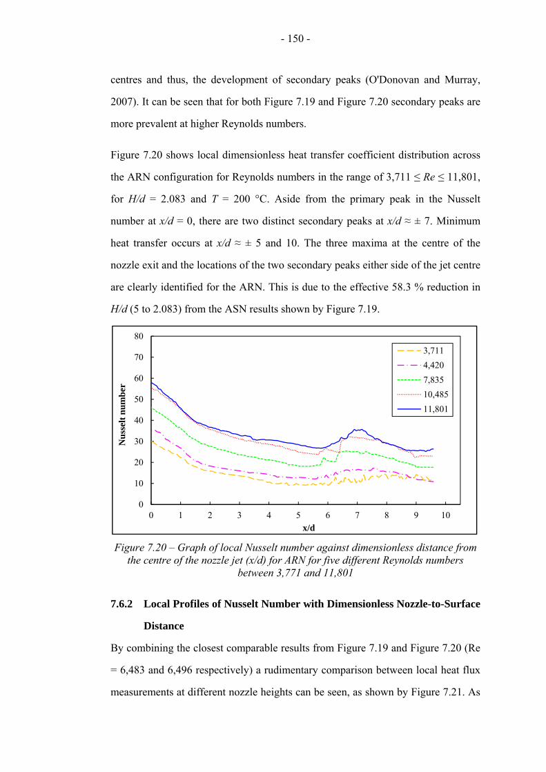
- 150 -

centres and thus, the development of secondary peaks (O'Donovan and Murray,

2007). It can be seen that for both Figure 7.19 and Figure 7.20 secondary peaks are

more prevalent at higher Reynolds numbers.

Figure 7.20 shows local dimensionless heat transfer coefficient distribution across

the ARN configuration for Reynolds numbers in the range of 3,711 ≤ Re ≤ 11,801,

for H/d = 2.083 and T = 200 °C. Aside from the primary peak in the Nusselt

number at x/d = 0, there are two distinct secondary peaks at x/d ≈ ± 7. Minimum

heat transfer occurs at x/d ≈ ± 5 and 10. The three maxima at the centre of the

nozzle exit and the locations of the two secondary peaks either side of the jet centre

are clearly identified for the ARN. This is due to the effective 58.3 % reduction in

H/d (5 to 2.083) from the ASN results shown by Figure 7.19.

Figure 7.20 – Graph of local Nusselt number against dimensionless distance from the centre of the nozzle jet (x/d) for ARN for five different Reynolds numbers

between 3,771 and 11,801

7.6.2 Local Profiles of Nusselt Number with Dimensionless Nozzle-to-Surface

Distance

By combining the closest comparable results from Figure 7.19 and Figure 7.20 (Re

= 6,483 and 6,496 respectively) a rudimentary comparison between local heat flux

measurements at different nozzle heights can be seen, as shown by Figure 7.21. As

0

10

20

30

40

50

60

70

80

0 1 2 3 4 5 6 7 8 9 10

Nu

ssel

t n

um

ber

x/d

3,711

4,420

7,835

10,485

11,801

- 151 -

these results are from differing nozzle arrangements, they are not directly

comparable, but the clarity of the secondary peaks is improved when H/d is

decreased from 5 to 2.083.

Figure 7.21 – Graph of local Nusselt number against dimensionless distance from the centre of the nozzle jet (x/d) for two different nozzle types and H/d values

The local variation of Nusselt number for values 1.33 ≤ H/d ≤ 7.83 is shown by

Figure 7.22. The constant conditions for these experiments were: Re = 3,211, T =

200 °C and the set of nozzles used was the ARN.

Figure 7.22 – Graph of local Nusselt number against dimensionless distance from the centre of the nozzle jet (x/d) for different values of H/d for ARN

0

10

20

30

40

50

60

-25 -20 -15 -10 -5 0 5 10 15 20 25

Nu

ssel

t n

um

ber

x/d

H/d = 2.083Re = 6,49612 mm round nozzlesH/d = 5Re = 6,4835 mm slot nozzles

0

5

10

15

20

25

30

35

0 1 2 3 4 5 6 7 8 9 10

Nu

ssel

t n

um

ber

x/d

H/d = 1.333

H/d = 2.167

H/d = 3.667

H/d = 6.000

H/d = 7.833

- 152 -

It can be seen that for lower nozzle-to-surface distances, the Nusselt number has a

higher peak at x/d = 0, but these decrease more rapidly with increasing x/d. At x/d ≈

2.5 all the profiles converge and secondary peaks can be observed for x/d values of

between 4 and 6.

7.7 Optimisation of Heat Transfer Coefficient for Energy

Savings

Heat flux correlations can be used to model oven energy use by using a three-

dimensional conduction model to predict the bake time for a range of heat transfer

coefficients. The model used makes use of finite element analysis software,

COMSOL Multiphysics (COMSOL, 2012), to predict bake time and is described

fully in Khatir et al. (2012b).

Once bake time is deduced, the throughput of product can be predicted if the

capacity of the oven is known – for example if the bake time was 30 minutes

(1,800 s) for an oven with a capacity of 5,000 kg the throughput would be

5,000/1,800 = 2.78 kg/s. If the bake time were halved, the throughput would double

whilst the oven will require the same amount of energy per kg of product to heat

the dough, tins and conveyor, to gelatinise the starch and to evaporate the moisture

from the product. The other heat losses – such as those through the roof, walls and

exhaust, remain constant regardless of the oven throughput. The thermal energy

efficiency saving can be calculated by assuming that approximately 19 % of oven

heat is lost to ambient, using the methodology described by in Chapter 6. Therefore

for a faster bake time the specific energy loss is reduced linearly with bake time.

Whilst a faster bake allows throughput to increase, and thus thermal efficiency to

increase, the higher air velocity required to increase convective heat transfer results

in a larger electricity load to power recirculation fans to increase the pressure in the

air supply ducts. The energy required to operate the fans given a certain required

velocity can be estimated using Eq. (7.5):

- 153 -

∆ (7.5)

where ΔP is calculated using Bernoulli’s equation for a range of air velocities.

The relationship between air velocity and heat transfer coefficient is given by the

dimensionless correlation, Eq. (7.5). By balancing the heat saving (gas) with the

additional energy load to power the fans (electricity), the optimum convective heat

transfer coefficient for energy efficiency can be calculated – this graph is shown by

Figure 7.23. It can be seen that when the heat transfer coefficient increases above

40 W/(m2·K), there is a marked rise in electricity required to distribute the air.

Conversely, with small values for heat transfer coefficient, the heat losses to

ambient are more significant.

Figure 7.23 – Predicted specific oven gas and electricity use as a function of heat transfer coefficient

In terms of total specific energy in kJ/kg, the optimum value for heat transfer

coefficient occurs for hc = 35 W/(m2·K). Using these conditions, the energy model

gives specific energy savings based on using the reported value of hc = 10

W/(m2·K) (Rohsenow et al., 1998) of 41.8 kJ/kg, which is composed of using an

extra 2.9 kJ/kg of electricity in the fans to save 44.7 kJ/kg of heat losses to ambient.

The total energy saving is 5.20 % based on the fact that the energy needed to bake

0

50

100

150

200

250

300

350

400

0 10 20 30 40 50 60 70 80 90 100

Sp

ecif

ic e

ner

gy (

kJ/

kg)

Heat transfer coefficient (W/(m2·K))

Additional energy electricityHeat losses to ambientTotal energy

- 154 -

bread under typical operating conditions is at least 804 kJ/kg – as seen in section

6.7. Depending on whether bakeries wish to prioritise reducing their energy use,

financial cost of energy or carbon emissions may influence the measure used for

energy efficiency. The carbon and financial cost penalties for electricity are

currently greater than gas, meaning a lower value for heat transfer coefficient may

be preferable. The carbon dioxide equivalent emissions per kg production graph, as

shown in Figure 7.24, indicates an optimum value for lowering carbon emissions of

30 W/(m2·K), i.e. 5 W/(m2·K) lower than optimising for energy consumption.

Figure 7.24 – Predicted bread baking carbon emissions equivalent per kg as a function of heat transfer coefficient

7.8 Summary

The methods used in this study give a new approach for measuring heat transfer in

the baking industry, with both global and local heat transfer coefficients being

determined for a number of conditions relevant to direct-fired jet impingement

baking ovens. The careful specification and use of heat flux sensors has made it

possible to conduct these experiments.

The results show interesting findings that correlate well with previous literature

relating to air jet impingement heat transfer. The mean heat transfer results for

0

200

400

600

800

1000

1200

1400

0 10 20 30 40 50 60 70 80 90 100

kg

CO

2e e

mis

sion

s p

er t

onn

e p

rod

uct

Heat transfer coefficient (W/(m2·K))

Total emissions

Additional emissions due to electricity

Additional emissions due to gas

- 155 -

ASN match closely with correlations proposed by Das et al. (1985) and Martin

(1977). The ARN configuration was unique because of the asymmetric distribution

of nozzles. The heat transfer characteristics were similar to the equivalent ASN

correlations but not the symmetric ARN correlations proposed by (Martin, 1977).

The mean dimensionless heat transfer coefficient (Nu) varies considerably under

different regimes. This demonstrates the importance of experimental measurements

to compare a specific regime to one of the many mean Nusselt number correlations

that exist in literature. Interestingly, the ARN configuration, where there is a large

degree of asymmetry of hole distribution can be effectively correlated as an ASN

by using the relative nozzle area, f, to calculate the equivalent slot width.

Local heat flux variations also exhibit interesting behaviours that should be

understood when designing commercial bread baking ovens. The effect of variation

in nozzle-to-surface distance can have little effect on the mean heat transfer, but

locally the effect across the profile of a nozzle can be of importance. Local heat

flux profiles also showed the prevalence of secondary peaks in a number of cases.

The magnitude of these secondary peaks was greater for high air velocities and low

H/d ratios

Using the experimental results, it was possible to estimate the optimum value for

heat transfer coefficient with relation to energy usage. It was found that by using hc

= 35 W/(m2·K), energy use could be reduced by over 5 %. The results presented in

this chapter may be of use to oven designers and bakery operators when selecting

conditions for bread baking to maximise heat transfer. Increasing the rate of heat

transfer could have a direct effect on lowering the baking time and therefore

improving plant efficiency and reducing energy usage and carbon emissions.

- 156 -

Chapter 8

Conclusions and Further Work

This thesis presents research focussed on analysing energy utilisation in

commercial bread baking – a manufacturing process that is responsible for

significant carbon emissions and environmental impact – with yearly energy usage

totalling 2,000 GWh and carbon emissions of 570,000 TCO2/year in the UK alone.

This research has been conducted in collaboration with industrial partners

Warburtons Limited, Spooner Industries Ltd. and SKM Enviros. Prior to the

commencement of this research, comparatively few studies have addressed end-use

energy demand and carbon emissions in the bread industry. Reasons for this

include: the relatively low cost of energy supply until recent times, food quality/

hygiene concerns of changing the production process and the traditional nature of

the industry.

This thesis challenges some of the ingrained and inherently inefficient commercial

practices used in the manufacture of bread. It provides rigorous scientific

justification and analysis tools to drive change in an important and large-scale

industry. These analysis tools have been actively used by industry in an attempt to

reduce energy use in the bread industry. This chapter provides a summary of the

contributions to new scientific understanding, methodologies, findings and key

conclusions that this research has provided.

8.1 Conclusions and Main Contributions to Scientific

Understanding

8.1.1 Computational Fluid Dynamic Analysis of Bread Provers

This study is the first attempt to analyse airflow within industrial bread provers

with the aim to reduce energy usage. Non-invasive measurement and predictive

techniques, such as CFD, are particularly pertinent when assessing bakery

- 157 -

equipment, as disruption to the manufacturing processes can be financially

expensive and leave the potential to cause food quality/ safety breaches. CFD has

been used for the first time to mitigate the detrimental impact that direct

measurements have to improve the energy efficiency of the bread proving phase.

The number of air changes is the practical parameter bakeries use to ensure

important food safety criteria are adhered to. A parametric study using ten different

cases for air changes between 10/hr and 100/hr was used to predict airflow within

the prover. Residence time analysis has shown the time taken for each individual

particle out of 2,000 injected to leave the prover cavity. Experimental

measurements of air velocity at the vent exits were obtained to validate the CFD

predictions, providing the validation and credibility needed to encourage

commercial bakeries to reduce the number of air changes.

It has been shown that for the proving process, the number of air changes can be

reduced by at least a third, from the previous level of 90/hr to 60/hr, without

breaching any current legislative or quality-driven standards. This reduction will

reduce the electricity demand of the prover air handling units by over 70 %. In

addition, it is anticipated that fewer air changes will mean the prover retains heat

and humidity, leading to reductions in the steam and gas burner energy demand.

The results of the CFD simulations have been used by bread manufacturers to

benchmark the number of air changes in industrial provers across a number of UK

bakeries. Furthermore, it has been suggested that the results could be used to

formulate a universal standard that would encourage bakeries to operate provers

under more energy efficient conditions.

8.1.2 System-Level Modelling of Industrial Bread Baking Ovens

Energy system modelling is a well-documented methodology that is used to predict

and measure energy streams. System models can lead to improvements in process

efficiency since they take into account the key influences affecting energy.

Initially, a system diagram of energy and material flows into and out of the oven

- 158 -

was generated, with reference to several different oven types, both indirect-fired

and direct-fired. Measurements of fundamental flow characteristics in a baking

oven, such as air velocity and temperature, were conducted to characterise oven

behaviour and provide parameters to be input into the system model. This

facilitated the formulation of the governing equations necessary to drive the

system-level model.

Thermal imaging, another form of non-invasive measurement, enabled surface

temperature profiles to be established at places that were difficult to access. Careful

configuration of the thermal imaging devices and software allowed reliable surface

plots of temperature distribution to be generated, which were then used to estimate

energy losses from the oven.

The results were verified by performing a sensitivity analysis on the model, which

used two separate scenarios to calculate the potential error. Firstly, each input to

the model was varied by ± 10 % to show the effect this had on the output results

and it was found that the variation of the majority of the outputs were within the

range expected for a model of this type. Secondly, each input was varied by the

expected accuracy of the measurement/ equipment used; again this showed

accuracy to be sufficient to allow reliable interpretation of the results. The results

of the analysis showed that energy use in bread baking can be reduced by 1.9 %.

This energy saving on a large scale is significant, as explained in Paton et al.

(2012b) the annual cost saving is estimated to be at least £0.5 million and carbon

savings of more than 5,000 tonnes CO2 equivalent for UK industry.

Energy system modelling is an increasingly popular technique that can be used to

flexibly analyse energy flow streams. The work presented here uses a system

model encompassed into a software framework that aims to provide direct benefit

to the bread industry as well as unique contributions to the scientific community.

The combination of novel measurement techniques to assess heat losses in

- 159 -

conjunction with a set of equations that can analyse the oven as a system has never

been done before for the bread industry, and builds upon previous studies in other

industries, both food and otherwise. The model has been used widely in industry to

benchmark and predict energy utilisation of commercial ovens, and by equipment

designers to identify opportunities for manufacturing the next generation of energy

efficient baking ovens.

8.1.3 Experimental Measurements for Air Jet Impingement Heat Transfer

for Regimes Relevant to Bread Baking

The novel experimental results showing mean and local heat transfer characteristics

for jet impingement nozzles under conditions applicable to the baking industry are

a valuable contribution of knowledge in the field of jet impingement heat transfer.

Furthermore, the correlations developed can prove useful to commercial oven

designers for developing a new generation of bread ovens where heat transfer can

be optimised in terms of jet velocity and nozzle dimensions. Much of the previous

experimental work carried out in this field was of little relevance to process

engineers, largely due to the types of nozzles used. Consequently, the experiments

described in this thesis intentionally used scaled-down industrially relevant

apparatus, which has enhanced the applicability of the methodologies and results.

The pilot oven facility enabled a wide range of conditions to be tested. The

apparatus ensured the flow represented conditions commonly experienced in

industrial baking and a turbulent regime under steady state conditions could be

maintained. A commercially available heat flux sensor was used for this, which

could measure convective and total heat transfer for typical conditions experienced

in bread baking ovens.

The mean heat transfer results agreed well with the seminal correlations of Martin

(1977), which give credibility and validation to the results. The experimental

evidence substantiates the assumption of the industry that asymmetric banks of

round nozzles can be approximated as slot nozzles. This insight could prove

- 160 -

especially significant as it means that mean heat transfer rates for arrays of both

round and slot nozzles can be modelled in two-dimensions, thereby reducing the

complexity of analysis and the corresponding computational requirements.

Theoretical optimisation of the heat transfer coefficient was conducted by

balancing the additional electricity load required to increase air velocity with the

subsequent reduction is baking time (and thus ambient heat losses per kg of bread)

made possible as a result of higher heat transfer rates. It was found that increasing

hc from the industry standard value of 10 to 35 W/(m2·K) resulted in energy

savings of over 5 %. This saving equates to over 75,000 tonnes CO2 equivalent per

year worldwide. This is a key finding that can help encourage the bread industry to

increase air velocity, depending on the effect on the product, in order to reduce

overall energy consumption. A further efficiency gain could be made if local

cogeneration (combined heat and power) could be made feasible to meet bakery

energy demand.

8.2 Future Work

The work presented in this thesis is not only relevant to the baking industry, but

covers technologies that are used in a number of other drying industries. The future

work that has been identified in this section reflects the adaptability of some of the

analysis techniques to identify energy savings in the bread industry.

8.2.1 Prover

In order to measure the energy savings that have been made possible as a result of

the CFD analysis presented in this thesis, a regression analysis of year-on-year

energy use would be necessary. This would help to substantiate the scale of energy

savings that have been estimated. Based on the magnitude of the energy savings for

using a lower number of air changes, it may be advisable to rethink prover design

and/ or retrofit technology in order to downsize the prover heating system (gas

burners) and review the sizing of air handling units based on worst-case scenarios.

- 161 -

Further optimisation of airflow within the prover could be conducted using a CFD

design optimisation study. Formal design optimisation, using methods such as

genetic programming, is a computational approach used to find an optimal solution

to an engineering problem. For multi-objective design optimisation, design

variables are identified, which in the case of the prover could be factors such as: the

number of air changes, the pitch between outlet vents, the size or shape of the

outlet vents, the distribution of tins within the prover, positioning of inlet/ outlet

ducts, air humidity etc. With current techniques, it is usually feasible to have no

more than 3-4 design variables, therefore the specification of the problem would

need to identify which variables are most practically varied and that are going to

have the greatest impact on energy usage. The objective function should define the

parameter to be maximised or minimised. For the prover, minimising the energy

use would be the objective function, but with a set of critical quality objectives that

would be required to ensure product quality and food safety. A simple graph shown

by Figure 8.1 characterises a Pareto front, where a trade-off between two variables

can be made. For this application, quality is a non-negotiable variable, therefore the

critical value must be maintained – the related costs can then the estimated. Such

approaches have been carried out in bread ovens.

Figure 8.1 – Example of a Pareto front showing competing objectives: the objective function, minimising cost (blue) and a critical quality objective (red)

Cos

t va

riab

le (

£/k

g)

Qu

alit

y va

riab

le (

% c

han

ce o

f b

reac

h)

Design variable

- 162 -

Figure 8.2 displays the three-dimensional surface response of the impact of two

design variables, H/d and unoz, on the objective function, temperature uniformity

(σT), for an industrial bread oven (Khatir et al., 2011b).

Figure 8.2 – Surface response of CFD optimisation study for optimising airflow in and industrial bread oven (Khatir et al., 2013, Khatir et al., 2012d)

8.2.2 Oven

The thermodynamic system-level model has been distributed and widely used in

Warburtons’ bakeries, the second largest grocery brand in the UK after Coca-Cola

(Phillips, 2011). Whilst the fundamental principles behind the analysis does not

change, as the software has evolved slight modifications have been made to the

governing equations – either to improve the accuracy, increase the ease of

operation or to simplify the methodology. It will be important for the legacy of the

model to continue maintenance on the software. The model could also be expanded

to form a life cycle assessment framework, where the cradle-to-grave

environmental impact of bread production could be assessed by a bakery operator

in a straightforward manner. The model will help industry to track improvements in

energy efficiency as advances are made to baking oven technology, therefore

continual use will help to highlight the change in energy utilisation as a result of

process enhancements.

- 163 -

One particular area for improvement identified as a result of the aforementioned

model, is in reducing the amount of heat being exhausted to atmosphere in flue

gases. There are three ways to increase efficiency in this area. Firstly, reducing the

flow rate of flue gases exhausted – this has been dismissed by industry, as a

minimum portion of combustion products need to be removed from the oven to

maintain safe manufacturing conditions. Secondly, reusing the heat for another

process by directly pumping exhaust gases to another process – for example in the

sugar industry waste heat from CHP incinerators is used to help grow tomatoes

(Stark and Jarvis, 2009). Thirdly, using heat exchangers to transfer the energy from

the waste flue gases to another form (solid, liquid or gas) to be used in another

operation – for example in washing tins. None of these options have been

implemented successfully despite numerous attempts over the years. However,

advances in heat exchanger efficiency and reliability mean there is increased

optimism that a commercially viable heat exchanger may be manufactured to

recover heat from oven exhausts in the short-term future.

Experimentation on heat transfer is a subject that can never be exhausted. The

range of different operating conditions that are possible is virtually limitless.

Although the subject of jet impingement heat transfer has been extensively covered

by literature, there is no method that is totally reliable for assessing heat transfer,

other than direct experimental measurement. Despite this, due to the expense of

preparing meticulous experimental setups and conducting careful measurements, it

is often more effective to use heat transfer correlations. Though it is clear that some

of the correlations are applicable, it has also been found correlations are lacking in

certain areas of parameter space – such as those used in bread baking. There has

been little experimentation relating to analysing the proportion of convection and

radiation with respect to air velocity based on measurements. This is a correlation

that could be developed but would potentially be highly dependent on the apparatus

used. Further studies could assess this by using different oven materials and

- 164 -

geometries to identify the relative ratio of convective to radiative heat transfer for

different systems. Further investigation into how rows of asymmetric round nozzles

can be approximated as slot nozzles would formulate completely novel research.

Deeper understanding of this phenomenon would add to scientific knowledge and

help designers of jet impingement systems to engineer nozzles that are both energy

efficient and practical.

Design of a completely new generation of baking ovens that are energy efficient is

a current priority for the baking industry. To minimise the energy consumption of a

new design of oven, it will be important for the previous work on heat transfer

(such as that presented in this thesis) along with the practical design experience of

those in the industry to be considered.

8.2.3 Other Bakery Equipment

Due to the large energy requirement of dough mixing since the advent of the

Chorleywood Bread Process, there are significant challenges relating to minimising

the mechanical energy used in dough mixers. Mixing using the this method uses

approximately 5 % of the bakery energy load – in terms of financial cost this figure

is greater due to the relative costs of electricity in comparison to other primary

energy sources. As stated in the introduction to this thesis, some computational

modelling work has been carried out in an attempt to optimise the mixing process,

but further work can be done. A number of factors affect the mixing process

(Frank, 2009), including: ingredients, dough rheology and temperature. Measuring

the impact of these variables to produce dough with the same product

characteristics would form an interesting piece of research.

Formation of the dough into a loaf shape is another area where research can help to

drive forward innovation in the bread manufacturing process. Dough-pieces are

currently formed by flattening the dough into a thin sheet and rolling into a

cylinder, before folding this into two or four sections. Little investigation has been

- 165 -

conducted to experiment with different ways of shaping the dough. The benefits of

the technique described over shaping the dough into a sphere and stretching into a

loaf shape have not been scientifically justified. Likewise, inventive solutions such

as: layering thin sheets of dough into a loaf shaped stack, joining multiple cylinders

or forcing the dough through a nozzle are all possibilities for modernising the

dough formation phase of bread baking. The energy impact of dough formation is

relatively low compared to the baking, proving and mixing stages; however, the

way in which the dough is formed can also have an impact on other stages of the

bread-making process.

As discussed previously, there are several cooling technologies available in the

food industry, many of which have been trialled to varying extents in bread-

making. It is important to fully understand the comparative benefits of different

coolers in terms of: energy impact/ life cycle assessment, capital investment,

operating costs, product quality (for example moisture loss), reliability, space

requirements and ease of operation. Ideally this multi-objective trade-off analysis

would be conducted on a commercial scale, to present the strongest possible case

for the best technology to be universally adopted. However, it is unlikely that

commercial bakeries would be willing to take the financial and operational risk

necessary to acquire unproven equipment on a large scale. It would be more

realistic to work with cooler manufacturers to understand the bakery requirements,

optimise design and trial innovative technologies on a pilot-scale with the aim to

revolutionise the cooling process.

8.3 Summary

The bread manufacturing process is traditional by nature, and as such it has been

observed in literature and through collaboration with industry, that innovation has

been limited over the past half-century. Carbon emission legislation and spiralling

energy costs have encouraged bakeries and equipment suppliers to reduce the

- 166 -

environmental impact of their products. There is a significant challenge to do this

whilst maintaining the product characteristics that have made bread a staple food in

a modern society. Despite these barriers, opportunities for reducing energy

utilisation are plentiful. The main challenge is to take theoretical performance gains

and transform them into commercially viable opportunities for investment.

Operational changes to the bread proving process have been suggested, with

scientific substantiation obtained through CFD modelling techniques. Using

residence time theory to analyse ten cases for different numbers of air changes has

shown that bakeries can reduce prover AHU electricity consumption by an

estimated 70 % whilst maintaining critical food safety and performance

characteristics. Additional savings in natural gas and steam consumption will

follow from this and can be quantified retrospectively.

System-level energy analysis of bread ovens has analysed the heat streams within

commercial bread ovens, showing that around 40 to 50 % of heat in the oven is

wasted in losses to atmosphere. This novel approach has made benchmarking

possible for both direct and indirect-fired ovens to compare energy efficiency using

a scientifically rigorous framework. Furthermore, the results highlight opportunities

for energy savings to be made – most notably in recovering waste heat from

exhaust gases, improving oven insulation to reduce the wall/ roof losses and

reducing energy losses from the conveyor.

Experimental measurements of heat flux for nozzles and temperature/ velocity

conditions relevant to the baking industry have corroborated many of the

previously published correlations. Unique data on the proportion of convection and

radiation shows, as expected, that the degree of convection is proportional to the jet

velocity. Furthermore, local heat flux profiles of air jets have shown interesting

behaviours that can be useful for oven designers. The prevalence of secondary

peaks, which were more noticeable for round nozzles that slots, is an interesting

- 167 -

result and can be explained by the effect of a decrease in nozzle-to-surface distance

due to the way the airflow develops for impinging jets.

As bread is a staple food product across most of the globe it is important to keep

availability high and retail prices low. The future prosperity of the bread baking

industry is increasingly dependent on lowering the cost of manufacture. Recent

years have seen the price of raw ingredients (in particular wheat) escalate rapidly,

due to poor harvests in the UK, Canada and USA, squeezing profit margins of

commercial bakers. Moreover, the fact that raw ingredients can be bought and sold

as stocks in a commodities market can have a further negative impact when there

are shortages of these ingredients.

The main costs in an industrial bakery aside from raw materials are: capital

expenditure, maintenance, staffing and energy. Of these four factors, capital

expenditure is often necessary to improve process efficiency, maintenance is

essential to avoid undue downtime and staffing levels have been reduced to an

absolute minimum through increased automation. Energy is the last remaining cost

that bakeries have largely neglected to address. The research presented here

explores energy utilisation in the commercial baking industry in order to help

mitigate the environmental impact and financial cost of bread manufacture. It is

envisaged that this research will help secure the long-term commercial and

environmental viability of one of the most historic and important of all industries.

- 168 -

References

AHRNE, L., ANDERSSON, C. G., FLOBERG, P., ROSEN, J. & LINGNERT, H. 2007. Effect of Crust Temperature and Water Content on Acrylamide Formation During Baking of White Bread: Steam and Falling Temperature Baking. LWT - Food Science and Technology. 40(10), pp. 1708-1715.

AIAA. 1998. Guide for the Verification and Validation of Computational Fluid Dynamics Simulations (G-077-1998e). Washington D.C.: American Institute of Aeronautics and Astronautics.

AKSYUTOV, L. N. 1974. Normal Spectral Emissivity of Gold, Platinum, and Tungsten. Journal of Engineering Physics and Thermophysics. 27(2), pp. 913-917.

ALTAMIRANO-FORTOUL, R., LE-BAIL, A., CHEVALLIER, S. & ROSELL, C. M. 2012. Effect of the Amount of Steam During Baking on Bread Crust Features and Water Diffusion. Journal of Food Engineering. 108(1), pp. 128-134.

ANDERSSON, B. J. 2012. Computational Fluid Dynamics for Engineers. Cambridge: Cambridge University Press.

ANDERSSON, K. & OHLSSON, T. 1999. Life Cycle Assessment of Bread Produced on Different Scales. The International Journal of Life Cycle Assessment. 4(1), pp. 25-40.

ANSYS INC. 2009. Ansys Fluent 12.0 in Workbench User's Guide. Canonsburg: ANSYS.

AUGUSTO, P. E. D., PINHEIRO, T. F. & CRISTIANINI, M. 2010. Using Computational Fluid-Dynamics (Cfd) for the Evaluation of Beer Pasteurization: Effect of Orientation of Cans. Ciência e Tecnologia de Alimentos. 30(4), pp. 980-986.

AZAR, K., ENGELBERTS, N., GOODMAN, C. W., HASKELL, M., LEI, N., JEGGEIS, Y., POURVASH, M. & TAVASSOLI, B. 2009. Qpedia Thermal Emagazine. Norwood: Advanced Thermal Solutions.

BACON, D. H. 1989. Basic Heat Transfer. London: Butterworth-Heinemann.

BAEHR, H. D. & STEPHAN, K. 1998. Heat and Mass Transfer. New York: Springer.

BAIK, O. D., GRABOWSKI, S., TRIGUI, M., MARCOTTE, M. & CASTAIGNE, F. 1999. Heat Transfer Coefficients on Cakes Baked in a Tunnel Type Industrial Oven. Journal of Food Science. 64(4), pp. 688-694.

BARDINA, J. E., HUANG, P. G. & COAKLEY, T. J. 1997. Turbulence Modeling Validation, Testing, and Development. NASA Technical Memorandum T110446. Moffett Field: Ames Research Center

BEECH, G. A. 1980. Energy Use in Bread Baking. Journal of the Science of Food and Agriculture. 31(3), pp. 289-298.

BEGGS, C. 2002. Energy: Management, Supply and Conservation. Oxford: Butterworth-Heinemann.

- 169 -

BENDING, R. & EDEN, R. J. 1984. Uk Energy: Structure, Prospects and Policies. Cambridge: Cambridge University Press.

BIRD, J. O. & ROSS, C. T. F. 2012. Mechanical Engineering Principles. New York, NY: Routledge.

BLANCHARD, G. H. 1965. The Blanchard Batter Process. Milling. 147 pp. 519-521.

BOULET, M., MARCOS, B., DOSTIE, M. & MORESOLI, C. 2010. Cfd Modeling of Heat Transfer and Flow Field in a Bakery Pilot Oven. Journal of Food Engineering. 97(3), pp. 393-402.

BRASCHKAT, J., PATYK, A., QUIRIN, M. & REINHARDT, G. A. 2003. Life Cycle Assessment of Bread Production - a Comparison of Eight Different Scenarios. In: Life Cycle Assessment in the Agri-food sector, 6-8 October 2003, Horsens, Denmark.

BREWSTER, M. Q. 1992. Thermal Radiative Transfer and Properties. Indianapolis: Wiley.

BRUMBAUGH, J. E. 2011. Audel Hvac Fundamentals Volume 3: Air Conditioning, Heat Pumps and Distribution Systems. Indianapolis: Wiley.

CAMPDEN & CHORLEYWOOD FOOD RESEARCH ASSOCIATION (CCFRA) & BRISTOL UNIVERSITY 2008. Utilisation of Waste Heat from Food Factories - Afm248br. CCFRA.

CARBON TRUST 2009. Conversion Factors: Energy and Carbon Conversions. London: Carbon Trust.

CARBON TRUST 2010. Industrial Energy Efficiency Accelerator: Guide to the Industrial Bakery Sector. London: Carbon Trust.

CARBON TRUST 2012a. Steam and High Temperature Hot Water Boilers: Introducing Energy Saving Opportunities for Business. London: Carbon Trust.

CARBON TRUST 2012b. Prices of Fuels Purchased by Manufacturing Industry. London: Department of Energy and Climate Change (DECC).

CARVALHO, M. D. & NOGUEIRA, M. 1997. Improvement of Energy Efficiency in Glass-Melting Furnaces, Cement Kilns and Baking Ovens. Applied Thermal Engineering. 17(8-10), pp. 921-933.

CASEY, M. & WINTERGERSTE, T. 2000. Best Practice Guidelines: Special Interest Group on "Quality and Trust in Industrial Cfd". London: European Research Community on Flow Turbulence and Combustion (ERCOFTAC).

CASPER, M. E. 1977. Energy-Saving Techniques for the Food Industry. Park Ridge: Noyes Data Corporation.

CAUVAIN, S. P. & YOUNG, L. S. 1998. Technology of Breadmaking. New York: Springer.

CAUVAIN, S. P. & YOUNG, L. S. 2006. The Chorleywood Bread Process. Boca Raton: CRC Press.

- 170 -

CHAPMAN, P. F. 1975. Fuel's Paradise: Energy Options for Britain. Harmondsworth: Penguin.

CHEVALLIER, S., ZUNIGA, R. & LE-BAIL, A. 2012. Assessment of Bread Dough Expansion During Fermentation. Food and Bioprocess Technology. 5(2), pp. 609-617.

CHILDS, P. R. N., GREENWOOD, J. R. & LONG, C. A. 1999. Heat Flux Measurement Techniques. Proceedings of the Institution of Mechanical Engineers, Part C. 213(7), pp. 655-677.

CHIOTELLIS, E. & CAMPBELL, G. M. 2003a. Proving of Bread Dough Ii - Measurement of Gas Production and Retention. Food and Bioproducts Processing. 81(3), pp. 207-216.

CHIOTELLIS, E. & CAMPBELL, G. M. 2003b. Proving of Bread Dough I - Modelling the Evolution of the Bubble Size Distribution. Food and Bioproducts Processing. 81(3), pp. 194-206.

CHRISTENSEN, A. & SINGH, R. P. 1984. Energy Consumption in the Baking Industry. In: Third International Congress on Engineering and Food, 26-28 September 1983, Dublin, Republic of Ireland.

COKER, A. K. 2001. Modeling of Chemical Kinetics and Reactor Design. Boston: Gulf Professional Publishing.

COLUCCI, D. W. & VISKANTA, R. 1996. Effect of Nozzle Geometry on Local Convective Heat Transfer to a Confined Impinging Air Jet. Experimental Thermal and Fluid Science. 13(1), pp. 71-80.

COMSOL. 2012. Comsol Multiphysics Installation and Operations Guide. Burlington: COMSOL AB.

CORDOBA, A. 2010. Quantitative Fit of a Model for Proving of Bread Dough and Determination of Dough Properties. Journal of Food Engineering. 96(3), pp. 440-448.

CVERNA, F. 2002. Thermal Properties of Metals. Ohio: ASM International.

DANCKWERTS, P. V. 1953. Continuous Flow Systems. Distribution of Residence Times. Chemical Engineering Science. 2(1), pp. 1-13.

DAS, D., DOUGLAS, W. J. M. & CROTOGINO, R. H. 1985. Convective Heat Transfer under Turbulent Impinging Slot Jet Nozzles at Large Temperature Differences. In: TOEI, R. & MAJUMDAR, A. S., (eds.). Drying '85. New York: Hemisphere.

DATAMONITOR 2011a. Bread & Rolls Industry Profile: United Kingdom. Bread & Rolls Industry Profile: United Kingdom. London: Datamonitor.

DATAMONITOR 2011b. Bread & Rolls Industry Profile: Global. Bread & Rolls Industry Profile: Global. London: Datamonitor.

DEPARTMENT OF ENERGY AND CLIMATE CHANGE 2012. Uk Emissions Statistics - 2011 Provisional Uk Figures: Data Tables. London: Department of Energy and Climate Change (DECC).

- 171 -

DILLER, T. E. 1993. Advances in Heat Flux Measurements. In: HARTNETT, J. P., IRVINE, T. F. & CHO, Y. I., (eds.). Advances in Heat Transfer. San Diego: Academic Press.

DONALD F. YOUNG, BRUCE R. MUNSON, THEODORE H. OKIISHI & HUEBSCH, W. W. 2010. A Brief Introduction to Fluid Mechanics, 5th Edition. Hoboken: Wiley.

DURBIN, P. A. 1996. On the K-Ε Stagnation Point Anomaly. International Journal of Heat and Fluid Flow. 17(1), pp. 89-90.

EARLE, R. L. 2004. Unit Operations in Food Processing: Web Edition. Palmerston North: The New Zealand Institute of Food Science & Technology.

ECKERT, E. R. G. 1959. Heat and Mass Transfer. New York: McGraw-Hill.

ERDOĞDU, F. & ANDERSON, B. 2010. Impingement Thermal Processing. In: FARID, M. M., (ed.) Mathematical Modeling of Food Processing. Boca Raton: CRC Press.

EUROPEAN COMMISSION JOINT RESEARCH CENTRE: INSTITUTE FOR ENVIRONMENT AND SUSTAINABILITY. 2010. International Reference Life Cycle Data System (Ilcd) Handbook - General Guide for Life Cycle Assessment - Detailed Guidance (Eur 24708 En). Luxembourg: Publications Office of the European Union.

FALKOVICH, G. 2011. Fluid Mechanics: A Short Course for Physicists. Cambridge: Cambridge University Press.

FELLOWS, P. J. 2009. Food Processing Technology Principles and Practice. Boca Raton: Woodhead Publishing.

FESSAS, D. & SCHIRALDI, A. 2000. Starch Gelatinization Kinetics in Bread Dough - Dsc Investigations on 'Simulated' Baking Processes. Journal of Thermal Analysis and Calorimetry. 61(2), pp. 411-423.

FITZGERALD, J. A. & GARIMELLA, S. V. 1998. A Study of the Flow Field of a Confined and Submerged Impinging Jet. International Journal of Heat and Mass Transfer. 41(8-9), pp. 1025-1034.

FRANK, P. 2009. Energy Efficiency Yields High Return on Investment. Baking Management [online] 1 June 2009. http://baking-management.com [Accessed on: 30 October 2012].

FUHRMANN, E., SOCKEL, H. & STEINRUCK, P. 1984. Improvement of Continuous Baking Ovens Efficiency. Journal of Wind Engineering and Industrial Aerodynamics. 16(2-3), pp. 201-212.

GARDON, R. & AKFIRAT, J. C. 1966. Heat Transfer Characteristics of Impinging Two-Dimensional Air Jets. Journal of Heat Transfer. 88(1), pp. 101-107.

GEERS, L. F. G., TUMMERS, M. J. & HANJALIC, K. 2004. Experimental Investigation of Impinging Jet Arrays. Experiments in Fluids. 36(6), pp. 946-958.

GELINAS, P. 2006. Yeast. In: HUI, Y. H., (ed.) Bakery Products: Science and Technology. Ames: Blackwell.

- 172 -

GHANI, A. G. A., FARID, M. M., CHEN, X. D. & RICHARDS, P. 1999a. Numerical Simulation of Natural Convection Heating of Canned Food by Computational Fluid Dynamics. Journal of Food Engineering. 41(1), pp. 55-64.

GHANI, A. G. A., FARID, M. M., CHEN, X. D. & RICHARDS, P. 1999b. An Investigation of Deactivation of Bacteria in a Canned Liquid Food During Sterilization Using Computational Fluid Dynamics (Cfd). Journal of Food Engineering. 42(4), pp. 207-214.

GOTTSCHALK, C. M. 1996. Industrial Energy Conservation. Chichester: Wiley.

GRENIER, A., LUCAS, T., COLLEWET, G. & LE BAIL, A. 2003. Assessment by Mri of Local Porosity in Dough During Proving. Theoretical Considerations and Experimental Validation Using a Spin-Echo Sequence. Magnetic Resonance Imaging. 21(9), pp. 1071-1086.

GRENIER, A., LUCAS, T., DAVENEL, A., COLLEWET, G. & LE BAIL, A. 2006. Comparison of Two Sequences: Spin-Echo and Gradient Echo for the Assessment of Dough Porosity During Proving. In: BELTON, P. S., GIL, A. M., WEBB, G. A. & RUTLEDGE, D., (eds.). Magnetic Resonance in Food Science: Latest Developments. Cambridge: The Royal Society of Chemistry.

GRENIER, D., LUCAS, T. & LE RAY, D. 2010. Measurement of Local Pressure During Proving of Bread Dough Sticks: Contribution of Surface Tension and Dough Viscosity to Gas Pressure in Bubbles. Journal of Cereal Science. 52(3), pp. 373-377.

GUPTA, T. R. 2001. Individual Heat Transfer Modes During Contact Baking of Indian Unleavened Flat Bread (Chapati) in a Continuous Oven. Journal of Food Engineering. 47(4), pp. 313-319.

HAMDAMI, N., MONTEAU, J. Y. & LE BAIL, A. 2004. Heat and Mass Transfer in Par-Baked Bread During Freezing. Food Research International. 37(5), pp. 477-488.

HANSEN, S. J. & BROWN, J. W. 2004. Investment Grade Energy Audit: Making Smart Energy Choices. Lilburn: Fairmont Press.

HARDISTY, H. & CAN, M. 1983. An Experimental Investigation into the Effect of Changes in the Geometry of a Slot Nozzle on the Heat-Transfer Characteristics of an Impinging Air Jet. Proceedings of the Institution of Mechanical Engineers, Part C. 197 pp. 7-15.

HARLOW, F. H. & WELCH, J. E. 1965. Numerical Calculation of Time-Dependent Viscous Incompressible Flow of Fluid with Free Surface. Physics of Fluids. 8(12), pp. 2182-2189.

HARLOW, F. H. & NAKAYAMA, P. I. 1967. Turbulence Transport Equations. Physics of Fluids. 10(11), pp. 2323-2332.

HOLDERBEKE, M. V., SANJUÁN, N., GEERKEN, T. & VOOGHT, D. D. 2003. The History of Bread Production: Using Lca in the Past. In: Life Cycle Assessment in the Agri-food sector, 6-8 October 2003, Horsens, Denmark.

HOLMAN, J. P. 2002. Heat Transfer. Boston: McGraw-Hill.

HUKSEFLUX THERMAL SENSORS c. 2010. Rc01 Manual V1004.

- 173 -

IBARRA-CASTANEDO, C., GONZALEZ, D., KLEIN, M., PILLA, M., VALLERAND, S. & MALDAGUE, X. 2004. Infrared Image Processing and Data Analysis. Infrared Physics & Technology. 46(1-2), pp. 75-83.

INCROPERA, F. P. & DEWITT, D. P. 2007. Fundamentals of Heat and Mass Transfer. Hoboken: Wiley.

INGOLD, B. J. 2008. Selecting a Nondestructive Testing Method, Part Vi: Thermal/Infrared Inspection Techniques – Thermography. Advanced Materials, Manufacturing, and Testing Information Analysis Center Quarterly. 3(2), pp. 9-12.

INTERNATIONAL ORGANIZATION FOR STANDARDIZATION. 2006a. Environmental Management - Life Cycle Assessment - Requirements and Guidelines. ISO 14044:2006.

INTERNATIONAL ORGANIZATION FOR STANDARDIZATION. 2006b. Environmental Management - Life Cycle Assessment - Principles and Framework. ISO 14040:2006.

JACOB, H. E., WINSTON, R. & WINSTON, C. 1944. Six Thousand Years of Bread, Its Holy and Unholy History. Garden City: Doubleday, Doran and Company.

JAHNKE, J. A. 2000. Continuous Emission Monitoring. New York: Wiley.

JAMES, S. J. & JAMES, C. 2011. The Potential of Ambient Cooling Systems for Reducing Refrigeration Loads and Saving Energy. In: International Congress on Engineering and Food, May 22-26 2011, Athens, Greece.

JOHNSON, L. A. & HOOVER, W. J. 1977. Energy Use in Baking Bread. Bakers Digest. 51 pp. 58-65.

KADISH, A. 1996. The Corn Laws: The Formation of Popular Economics in Britain. London: Pickering and Chatto.

KANNAN, R. & BOIE, W. 2003. Energy Management Practices in Sme - Case Study of a Bakery in Germany. Energy Conversion and Management. 44(6), pp. 945-959.

KAUSHAL, P. & SHARMA, H. K. 2012. Concept of Computational Fluid Dynamics (Cfd) and Its Applications in Food Processing Equipment Design Journal of Food Processing and Technology. 3(1), pp. 1-7.

KAWAGUTI, M. 1953. Numerical Solution of the Navier-Stokes Equations for the Flow around a Circular Cylinder at Reynolds Number = 40. Journal of the Physical Society of Japan. 8(6), pp. 747-757.

KENT, J. 2012. Our Daily Bread: A Half-Baked History. BBC Radio 4. 21 May 2012.

KHATIR, Z., PATON, J. B., THOMPSON, H. M., KAPUR, N., TOROPOV, V. V., LAWES, M. & KIRK, D. 2010. Computational Fluid Dynamics (Cfd) Investigation of Air Flow and Temperature Distribution in a Small Scale Bread-Baking Oven. In: Sustainable Thermal Energy Management Conference (SusTEM2010), 3-4 November 2010, Newcastle, UK.

KHATIR, Z., THOMPSON, H. M., KAPUR, N., TOROPOV, V. V. & PATON, J. B. 2011a. The Application of Computational Fluid Dynamics and Design

- 174 -

Optimisation in the British Bread-Baking Industry. In: The 8th International Conference on CFD in Oil & Gas, Metallurgical and Process Industries (SINTEF/NTNU), 21-23 June 2011, Trondheim, Norway.

KHATIR, Z., THOMPSON, H. M., KAPUR, N., TOROPOV, V. V. & PATON, J. B. 2011b. Multi-Objective Computational Fluid Dynamics (Cfd) Design Optimisation in Commercial Bread-Baking. In: The Twelfth UK National Heat Transfer Conference (UKHTC 2011), 30 Aug-1 Sept 2011, Leeds, UK.

KHATIR, Z., PATON, J. B., THOMPSON, H. M., KAPUR, N. & TOROPOV, V. V. 2012a. A Multi-Objective Design Methodology to Improve Energy Efficiency in the Bread-Baking Industry. In: 2012 EFFoST Annual Meeting, 20-23 November 2012, Montpellier, France.

KHATIR, Z., PATON, J. B., THOMPSON, H. M., KAPUR, N. & TOROPOV, V. V. 2012b. Opportunities for Energy Savings by Experimental and Numerical Analysis of the Bread Baking Process. In: The 4th International Conference on Applied Energy (ICAE 2012), 5-8 July 2012, Suzhou, China.

KHATIR, Z., PATON, J. B., THOMPSON, H. M., KAPUR, N., TOROPOV, V. V., LAWES, M. & KIRK, D. 2012c. Computational Fluid Dynamics (Cfd) Investigation of Air Flow and Temperature Distribution in a Small Scale Bread-Baking Oven. Applied Energy. 89(1), pp. 89-96.

KHATIR, Z., THOMPSON, H. M., KAPUR, N., TOROPOV, V. V. & PATON, J. B. 2012d. Multi-Objective Computational Fluid Dynamics (Cfd) Design Optimisation in Commercial Bread-Baking. Applied Thermal Engineering. DOI: 10.1016/j.applthermaleng.2012.08.011.

KHATIR, Z., PATON, J. B., THOMPSON, H. M., KAPUR, N. & TOROPOV, V. V. 2013. Optimisation of the Energy Efficiency of Bread-Baking Ovens Using a Combined Experimental and Computational Approach. Applied Energy. DOI: 10.1016/j.apenergy.2013.02.034.

KIRK, D. 2011. Spooner Industries Ltd., Personal communication.

KLEMES, J., SMITH, R. & KIM, J.-K. 2008. Handbook of Water and Energy Management in Food Processing. Boca Raton: Woodhead Publishing.

KONDJOYAN, A. & DAUDIN, J. D. 1997. Optimisation of Air-Flow Conditions During the Chilling and Storage of Carcasses and Meat Products. Journal of Food Engineering. 34(3), pp. 243-258.

KREITH, F. & GOSWAMI, Y. 2008. Energy Management and Conservation Handbook. Boca Raton: Taylor & Francis.

KREITH, F., MANGLIK, R. M., BOHN, M. & TIWARI, S. 2011. Principles of Heat Transfer. Stamford: Cengage Learning.

KRESS-ROGERS, E. & BRIMELOW, C. J. B. 2001. Instrumentation and Sensors for the Food Industry. Boca Raton: CRC Press.

LAUKKANEN, M. 1984. Improving Energy Use in Finnish Bakeries. In: Third International Congress on Engineering and Food, 26-28 September 1983, Dublin.

LAUNDER, B. E. & SPALDING, D. B. 1974. The Numerical Computation of Turbulent Flows. Computer Methods in Applied Mechanics and Engineering 3(2), pp. 269-289.

- 175 -

LE-BAIL, A., DESSEV, T., JURY, V., ZUNIGA, R., PARK, T. & PITROFF, M. 2010. Energy Demand for Selected Bread Making Processes: Conventional Versus Part Baked Frozen Technologies. Journal of Food Engineering. 96(4), pp. 510-519.

LEACH, G. 1975. Energy and Food Production. Food Policy. 1(1), pp. 62-73.

LI, A. & WALKER, C. E. 1996. Cake Baking in Conventional, Impingement and Hybrid Ovens. Journal of Food Science. 61(1), pp. 188-197.

LUCAS, T., GRENIER, D., BORNERT, M., CHALLOIS, S. & QUELLEC, S. 2010. Bubble Growth and Collapse in Pre-Fermented Doughs During Freezing, Thawing and Final Proving. Food Research International. 43(4), pp. 1041-1048.

LYTLE, D. & WEBB, B. W. 1994. Air Jet Impingement Heat Transfer at Low Nozzle-Plate Spacings. International Journal of Heat and Mass Transfer. 37(12), pp. 1687-1697.

MALDAGUE, X. 2001. Theory and Practice of Infrared Technology for Nondestructive Testing. New York: Wiley.

MARCOTTE, M. & GRABOWSKI, S. 2008. Minimising Energy Consumption Associated with Drying, Baking and Evaporation. In: KLEMES, J., SMITH, R. & KIM, J.-K., (eds.). Handbook of Water and Energy Management in Food Processing. Cambridge: Woodhead Publishing.

MARSON, A. D. 1999. Air Flotation Drying of Paper Pulp. Engineering Doctorate, University of Manchester.

MARTIN, H. 1977. Heat and Mass Transfer between Impinging Gas Jets and Solid Surfaces. Advances in Heat Transfer. 13 pp. 1-60.

MATTSSON, B. & SONESSON, U. 2003. Environmentally-Friendly Food Processing. Boca Raton: Woodhead Publishing.

MCADAMS, W. H. 1954. Heat Transmission. London: McGraw-Hill.

MCDONALD, K. & SUN, D. W. 2000. Vacuum Cooling Technology for the Food Processing Industry: A Review. Journal of Food Engineering. 45(2), pp. 55-65.

MENTER, F. R. 1994. Two-Equation Eddy-Viscosity Turbulence Models for Engineering Applications. AIAA Journal. 32(8), pp. 1598-1605.

MIDDEN, T. M. 1995. Impingement Air Baking for Snack Foods. Cereal Foods World. 40(8), pp. 532-535.

MIRADE, P. S. & DAUDIN, J. D. 2000. A Numerical Study of the Airflow Patterns in a Sausage Dryer. Drying Technology. 18(1-2), pp. 81-97.

MIRADE, P. S., DAUDIN, J. D., DUCEPT, F., TRYSTRAM, G. & CLEMENT, J. 2004. Characterization and Cfd Modelling of Air Temperature and Velocity Profiles in an Industrial Biscuit Baking Tunnel Oven. Food Research International. 37(10), pp. 1031-1039.

MISTRY, H., GANAPATHI-SUBBU, DEY, S., BISHNOI, P. & CASTILLO, J. L. 2006. Modeling of Transient Natural Convection Heat Transfer in Electric Ovens. Applied Thermal Engineering. 26(17-18), pp. 2448-2456.

- 176 -

MONTEAU, J. Y. 2008. Estimation of Thermal Conductivity of Sandwich Bread Using an Inverse Method. Journal of Food Engineering. 85(1), pp. 132-140.

MOREIRA, R. G. 2002. Impingement Drying Applications to Foods. In: 2002 IFT Annual Meeting & Food Expo, 16-19 June 2002, Anahein, California.

MUJUMDAR, A. S. 2007. Handbook of Industrial Drying. Boca Raton: Taylor & Francis.

NAVANEETHAKRISHNAN, P., SRINIVASAN, P. S. S. & DHANDAPANI, S. 2007. Heat Transfer and Heating Rate of Food Stuffs in Commercial Shop Ovens. Sadhana. 32(5), pp. 535-544.

NELLIS, G. & KLEIN, S. A. 2009. Heat Transfer. Cambridge: Cambridge University Press.

NITIN, N. & KARWE, M. V. 2001. Heat Transfer Coefficient for Cookie Shaped Objects in a Hot Air Jet Impingement Oven. Journal of Food Process Engineering. 24(1), pp. 51-69.

NORRIS, J. R., ABBOTT, M. T. & DOBIE, M. 2002. High Performance Air Impingement/Microwave Cooking Systems. In: 2002 IFT Annual Meeting & Food Expo, 16-19 June 2002, Anahein, California.

NORTON, T. & SUN, D.-W. 2006. Computational Fluid Dynamics (Cfd) - an Effective and Efficient Design and Analysis Tool for the Food Industry: A Review. Trends in Food Science & Technology. 17(11), pp. 600-620.

NORTON, T. & SUN, D.-W. 2007. An Overview of Cfd Applications in the Food Industry. In: SUN, D.-W., (ed.) Computational Fluid Dynamics in Food Processing. Boca Raton: Taylor & Francis.

O'DONOVAN, T. S. & MURRAY, D. B. 2007. Jet Impingement Heat Transfer - Part I: Mean and Root-Mean-Square Heat Transfer and Velocity Distributions. International Journal of Heat and Mass Transfer. 50(17-18), pp. 3291-3301.

OAKLEY, T. 2009. Warburtons Limited, Personal communication.

OBERKAMPF, W. L. & TRUCANO, T. G. 2002. Verification and Validation in Computational Fluid Dynamics. Progress in Aerospace Sciences. 38(3), pp. 209-272.

OLSSON, E. E. M., AHRNE, L. M. & TRÄGÅRDH, A. C. 2004. Heat Transfer from a Slot Air Jet Impinging on a Circular Cylinder. Journal of Food Engineering. 63(4), pp. 393-401.

OLSSON, E. E. M., AHRNE, L. M. & TRÄGÅRDH, A. C. 2005. Flow and Heat Transfer from Multiple Slot Air Jets Impinging on Circular Cylinders. Journal of Food Engineering. 67(3), pp. 273-280.

OLSSON, E. E. M. & TRÄGÅRDH, A. C. 2007. Cfd Modeling of Jet Impingement During Heating and Cooling of Foods. In: SUN, D.-W., (ed.) Computational Fluid Dynamics in Food Processing. Boca Raton: Taylor & Francis.

OPENCFD LTD. 2012. Openfoam - the Open Source Cfd Toolbox: User Guide. Bracknell: OpenFOAM Foundation.

- 177 -

OUSEGUI, A., MORESOLI, C., DOSTIE, M. & MARCOS, B. 2010. Porous Multiphase Approach for Baking Process - Explicit Formulation of Evaporation Rate. Journal of Food Engineering. 100(3), pp. 535-544.

OVADIA, D. Z. & WALKER, C. E. 1998. Impingement in Food Processing. Food Technology. 52(4), pp. 46-50.

OWEN, J. 2012. Passion for Artisan Bread Puts Wind in the Sails of Britain's Mills. The Independent [online] 13 May 2012. http://www.independent.co.uk [Accessed on: 30 October 2012].

PARK, J. & MACKAY, S. 2003. Practical Data Acquisition for Instrumentation and Control Systems. Oxford: Elsevier.

PATANKAR, S. V. & SPALDING, D. B. 1972. Calculation Procedure for Heat, Mass and Momentum-Transfer in Three-Dimensional Parabolic Flows. International Journal of Heat and Mass Transfer. 15(10), pp. 1787-1806.

PATON, J. B., KHATIR, Z., THOMPSON, H. M., KAPUR, N. & TOROPOV, V. V. 2011. Thermal Energy Management in the Bread-Baking Industry Using a System Modelling Approach. In: Sustainable Thermal Energy Management International Conference (SusTEM 2011), 25-26 Oct 2011, Newcastle upon Tyne, UK.

PATON, J. B., KHATIR, Z., KAPUR, N., THOMPSON, H. M. & TOROPOV, V. V. 2012a. An Experimental and Numerical Investigation of Industrial Bread Proving. In: 2012 EFFoST Annual Meeting, 20-23 November 2012, Montpellier, France.

PATON, J. B., KHATIR, Z., THOMPSON, H. M., KAPUR, N. & TOROPOV, V. V. 2012b. Thermal Energy Management in the Bread Baking Industry Using a System Modelling Approach. Applied Thermal Engineering. DOI: 10.1016/j.applthermaleng.2012.03.036.

PHILLIPS, B. 2011. The 100 Biggest Grocery Retailers in Britain. London: The Grocer.

PIMENTEL, D. & PIMENTEL, M. H. 2008. Food, Energy, and Society. Boca Raton: CRC Press.

POPE, S. B. 2000. Turbulent Flows. Cambridge: Cambridge University Press.

PRICE, I. 2012. Warburtons Limited, Personal communication.

PROBERT, D. & NEWBOROUGH, M. 1985. Designs, Thermal Performances and Other Factors Concerning Cooking Equipment and Associated Facilities. Applied Energy. 21(2–3), pp. 81-222.

PURLIS, E. & SALVADORI, V. O. 2009a. Bread Baking as a Moving Boundary Problem. Part 1: Mathematical Modelling. Journal of Food Engineering. 91(3), pp. 428-433.

PURLIS, E. & SALVADORI, V. O. 2009b. Bread Baking as a Moving Boundary Problem. Part 2: Model Validation and Numerical Simulation. Journal of Food Engineering. 91(3), pp. 434-442.

PURLIS, E. 2011. Bread Baking: Technological Considerations Based on Process Modelling and Simulation. Journal of Food Engineering. 103(1), pp. 92-102.

- 178 -

REBITZER, G., EKVALL, T., FRISCHKNECHT, R., HUNKELER, D., NORRIS, G., RYDBERG, T., SCHMIDT, W. P., SUH, S., WEIDEMA, B. P. & PENNINGTON, D. W. 2004. Life Cycle Assessment: Part 1: Framework, Goal and Scope Definition, Inventory Analysis, and Applications. Environment International. 30(5), pp. 701-720.

REVEDIN, A., ARANGUREN, B., BECATTINI, R., LONGO, L., MARCONI, E., LIPPI, M. M., SKAKUN, N., SINITSYN, A., SPIRIDONOVA, E. & SVOBODA, J. 2010. Thirty Thousand-Year-Old Evidence of Plant Food Processing. Proceedings of the National Academy of Sciences of the United States of America. 107(44), pp. 18815-18819.

RIBOTTA, P. D., LEON, A. E. & AÑÓN, M. C. 2001. Effect of Freezing and Frozen Storage of Doughs on Bread Quality. Journal of Agricultural and Food Chemistry. 49(2), pp. 913-918.

RICHARDSON, L. F. 1910. On the Approximate Arithmetical Solution by Finite Differences of Physical Problems Involving Differential Equations, with an Application to the Stresses in a Masonry Dam. Philosophical Transactions of the Royal Society of London Series A - Containing Papers of a Mathematical or Physical Character. 83(563), pp. 335-336.

RICHARDSON, L. F. 1922. Weather Prediction by Numerical Process. Cambridge: Cambridge University Press.

ROACHE, P. J. 1994. Perspective: A Method for Uniform Reporting of Grid Refinement Studies. Journal of Fluids Engineering. 116(3), pp. 405-413.

ROACHE, P. J. 1998. Verification and Validation in Computational Science and Engineering. Socorro: Hermosa.

ROBERTS, J. S., TONG, C. H. & LUND, D. B. 2002. Drying Kinetics and Time-Temperature Distribution of Pregelatinized Bread. Journal of Food Science. 67(3), pp. 1080-1087.

ROGERS, G. F. C. & MAYHEW, Y. R. 1988. Thermodynamic and Transport Properties of Fluids, Si Units. Oxford: Blackwell.

ROHSENOW, W. M., HARTNETT, J. P. & CHO, Y. I. 1998. Handbook of Heat Transfer. London: McGraw-Hill.

ROSING, L. & NIELSEN, A. M. 2003. When a Hole Matters - the Story of the Hole in a Bread for French Hotdog. In: Life Cycle Assessment in the Agri-food sector, 6-8 Oct 2003, Horsens, Denmark.

RUSSELL, T. W. F., ROBINSON, A. S. & WAGNER, N. J. 2008. Mass and Heat Transfer: Analysis of Mass Contactors and Heat Exchangers. Cambridge: Cambridge University Press.

SABLANI, S. S., MARCOTTE, M., BAIK, O. D. & CASTAIGNE, F. 1998. Modeling of Simultaneous Heat and Water Transport in the Baking Process. LWT - Food Science and Technology. 31(3), pp. 201-209.

SARKAR, A. & SINGH, R. P. 2004. Air Impingement Technology for Food Processing: Visualization Studies. LWT - Food Science and Technology. 37(8), pp. 873-879.

- 179 -

SATO, H., MATSUMURA, T. & SHIBUKAWA, S. 1987. Apparent Heat Transfer in a Forced Convection Oven and Properties of Baked Food. Journal of Food Science. 52(1), pp. 185-193.

SCOTT, G. & RICHARDSON, P. 1997. The Application of Computational Fluid Dynamics in the Food Industry. Trends in Food Science & Technology. 8(4), pp. 119-124.

ŠERUGA, B., BUDŽAKI, S. & UGARČIĆ-HARDI, Ž. 2007. Individual Heat Transfer Modes During Baking of “Mlinci” Dough. Agriculturae Conspectus Scientificus. 72(3), pp. 257-263.

SERWAY, R. A. & JEWETT, J. W. 2010. Physics for Scientists and Engineers, Volume 1. Pacific Grove: Brooks/Cole.

SHAH, P., CAMPBELL, G. M., MCKEE, S. L. & RIELLY, C. D. 1998. Proving of Bread Dough: Modelling the Growth of Individual Bubbles. Food and Bioproducts Processing. 76(2), pp. 73-79.

SHIBUKAWA, S., SUGIYAMA, K. & YANO, T. 1989. Effects of Heat Transfer by Radiation and Convection on Browning of Cookies at Baking. Journal of Food Science. 54(3), pp. 621-624.

SHIH, T. H., LIOU, W. W., SHABBIR, A., YANG, Z. G. & ZHU, J. 1995. A New K-Ε Eddy Viscosity Model for High Reynolds-Number Turbulent Flows. Computers & Fluids. 24(3), pp. 227-238.

SØRENSEN, B. 2011. Life-Cycle Analysis of Energy Systems: From Methodology to Applications. Cambridge: RSC Publishing.

STAFFORD, J., WALSH, E. & EGAN, V. 2009. Characterizing Convective Heat Transfer Using Infrared Thermography and the Heated-Thin-Foil Technique. Measurement Science & Technology. 20(10), pp. 1-11.

STARK, R. & JARVIS, P. 2009. Bioethanol from Sugar Beet and Horticultural Use of Surplus Process Heat. In: Meeting of the International Fertiliser Society, 2 April 2009, London, UK.

STEAR, C. A. 1990. Handbook of Breadmaking Technology. London: Elsevier.

STEPHAN, P. 1993. Vdi Heat Atlas. Dusseldorf: Springer.

SUMNU, S. G. & SAHIN, S. 2008. Food Engineering Aspects of Baking Sweet Goods. Boca Raton: CRC Press.

SUN, D.-W. 2007. Computational Fluid Dynamics in Food Processing. Boca Raton: Taylor & Francis.

TANNAHILL, R. 2002. Food in History. London: Broadway.

THE FEDERATION OF BAKERS 2010. Annual Report and List of Members 2010. London: The Federation of Bakers.

THERDTHAI, N., ZHOU, W. B. & ADAMCZAK, T. 2002. Optimisation of the Temperature Profile in Bread Baking. Journal of Food Engineering. 55(1), pp. 41-48.

- 180 -

THERDTHAI, N., ZHOU, W. B. & ADAMCZAK, T. 2003. Two-Dimensional Cfd Modelling and Simulation of an Industrial Continuous Bread Baking Oven. Journal of Food Engineering. 60(2), pp. 211-217.

THERDTHAI, N., ZHOU, W. B. & ADAMCZAK, T. 2004a. Three-Dimensional Cfd Modelling and Simulation of the Temperature Profiles and Airflow Patterns During a Continuous Industrial Baking Process. Journal of Food Engineering. 65(4), pp. 599-608.

THERDTHAI, N., ZHOU, W. B. & ADAMCZAK, T. 2004b. The Development of an Anemometer for Industrial Bread Baking. Journal of Food Engineering. 63(3), pp. 329-334.

THOM, A. 1933. The Flow Past Circular Cylinders at Low Speeds. Proceedings of the Royal Society of London Series A - Containing Papers of a Mathematical and Physical Character. 141(844), pp. 651-669.

THOMPSON, J. F., SONI, B. K. & WEATHERILL, N. P. 1999. Handbook of Grid Generation. London: CRC Press.

THUMANN, A. & YOUNGER, W. J. 2003. Handbook of Energy Audits. Lilburn: Fairmont Press.

THUMANN, A. & MEHTA, D. P. 2008. Handbook of Energy Engineering. Lilburn: Fairmont Press.

TU, J., YEOH, G. H. & LIU, C. 2008. Computational Fluid Dynamics: A Practical Approach. Oxford: Butterworth-Heinemann.

TURNER, W. C. 1993. Energy Management Handbook. Lilburn: Fairmont Press.

UNKLESBAY, N., UNKLESBAY, K., NAHAISI, M. & KRAUSE, G. 1981. Thermal Conductivity of White Bread During Convective Heat Processing. Journal of Food Science. 47 pp. 249-259.

VERBOVEN, P., SCHEERLINCK, N., DE BAERDEMAEKER, J. & NICOLAI, B. M. 2000a. Computational Fluid Dynamics Modelling and Validation of the Isothermal Airflow in a Forced Convection Oven. Journal of Food Engineering. 43(1), pp. 41-53.

VERBOVEN, P., SCHEERLINCK, N., DE BAERDEMAEKER, J. & NICOLAI, B. M. 2000b. Computational Fluid Dynamics Modelling and Validation of the Temperature Distribution in a Forced Convection Oven. Journal of Food Engineering. 43(2), pp. 61-73.

VERSTEEG, H. K. & MALALASEKERA, W. 2007. An Introduction to Computational Fluid Dynamics: The Finite Volume Method. Harlow: Prentice Hall.

WANG, L. & SUN, D.-W. 2003. Recent Developments in Numerical Modelling of Heating and Cooling Processes in the Food Industry: A Review. Trends in Food Science & Technology. 14(10), pp. 408-423.

WANG, L. J. & SUN, D. W. 2001. Rapid Cooling of Porous and Moisture Foods by Using Vacuum Cooling Technology. Trends in Food Science & Technology. 12(5-6), pp. 174-184.

WARD, I. 2010. Warburtons Limited, Personal communication.

- 181 -

WHITESIDE, R. L. 1982. Energy Use in the Baking Industry. Bakers Digest. 56(4), pp. 30-34.

WILCOX, D. C. 1988. Reassessment of the Scale-Determining Equation for Advanced Turbulence Models. AIAA Journal. 26(11), pp. 1299-1310.

WILLIAMSON, M. E. & WILSON, D. I. 2009. Development of an Improved Heating System for Industrial Tunnel Baking Ovens. Journal of Food Engineering. 91(1), pp. 64-71.

WIMBERGER, R. J. 1999. Convection Air Dryer Sizing and Section of Nozzle Design/ Spacing. In: TAPPI Polymers, Laminations & Coatings Conference, 22-26 Aug 1999, Atlanta, GA.

WONG, S. Y., ZHOU, W. B. & HUA, J. S. 2007. Cfd Modeling of an Industrial Continuous Bread-Baking Process Involving U-Movement. Journal of Food Engineering. 78(3), pp. 888-896.

WU, H., JOUHARA, H., TASSOU, S. A. & KARAYIANNIS, T. G. 2010. Modelling of Energy Flows in Potato Crisp Frying Processes. In: Sustainable Thermal Energy Management Conference (SusTEM2010), 3-4 Nov 2010, Newcastle, UK.

WU, H., JOUHARA, H., TASSOU, S. A. & KARAYIANNIS, T. G. 2012. Modelling of Energy Flows in Potato Crisp Frying Processes. Applied Energy. 89(1), pp. 81-88.

YAKHOT, V., ORSZAG, S. A., THANGAM, S., GATSKI, T. B. & SPEZIALE, C. G. 1992. Development of Turbulence Models for Shear Flows by a Double Expansion Technique. Physics of Fluids a-Fluid Dynamics. 4(7), pp. 1510-1520.

YANNIOTIS, S. 2008. Solving Problems in Food Engineering. New York: Springer.

YASUNAGA, T., BUSHUK, W. & IRVINE, G. N. 1968. Gelatinization of Starch During Bread-Baking. Cereal Chemistry. 45(3), pp. 269-279.

ZANONI, B., PERI, C. & BRUNO, D. 1995a. Modeling of Starch Gelatinization Kinetics of Bread Crumb During Baking. LWT - Food Science and Technology. 28(3), pp. 314-318.

ZANONI, B., SCHIRALDI, A. & SIMONETTA, R. 1995b. Naive Model of Starch Gelatinization Kinetics. Journal of Food Engineering. 24(1), pp. 25-33.

ZHANG, J. & DATTA, A. K. 2006. Mathematical Modeling of Bread Baking Process. Journal of Food Engineering. 75(1), pp. 78-89.

ZHOU, W. & THERDTHAI, N. 2007. Three-Dimensional Modeling of a Continuous Industrial Baking Process. In: SUN, D.-W., (ed.) Computational Fluid Dynamics in Food Processing. Boca Raton: Taylor & Francis.

ZIENKIEWICZ, O. C., TAYLOR, R. L. & ZHU, J. Z. 2005. The Finite Element Method Its Basis and Fundamentals. Oxford: Butterworth-Heinemann.

ZUCKERMAN, N. & LIOR, N. 2006. Jet Impingement Heat Transfer: Physics, Correlations, and Numerical Modeling. In: GREENE, G. A., CHO, Y. I., HARTNETT, J. P. & BAR-COHEN, A., (eds.). Advances in Heat Transfer Volume 39. London: Elsevier.

thesis joe paton - white rose university...

Documents