NAVAL POSTGRADUATE SCHOOL Monterey, California

THESIS

IMPLEMENTING THE CROSS AMBIGUITY FUNCTION AND GENERATING GEOMETRY-SPECIFIC SIGNALS

by

Joe J. Johnson

September 2001

Thesis Advisor: Herschel H. Loomis, Jr. Second Reader: Ralph D. Hippenstiel

Approved for public release; distribution is unlimited.

Report Documentation Page

Report Date 30 Sep 2001

Report Type N/A

Dates Covered (from... to) -

Title and Subtitle Implementing the Cross Ambiguity Function andGenerating Geometry-Specific Signals 6. AUTHOR(S)Joe J. Johnson

Contract Number

Grant Number

Program Element Number

Author(s) Joe J. Johnson

Project Number

Task Number

Work Unit Number

Performing Organization Name(s) and Address(es) Research Office Naval Postgraduate School Monterey,Ca 93943-5138

Performing Organization Report Number

Sponsoring/Monitoring Agency Name(s) and Address(es)

Sponsor/Monitor’s Acronym(s)

Sponsor/Monitor’s Report Number(s)

Distribution/Availability Statement Approved for public release, distribution unlimited

Supplementary Notes

Abstract

Subject Terms

Report Classification unclassified

Classification of this page unclassified

Classification of Abstract unclassified

Limitation of Abstract UU

Number of Pages 123

THIS PAGE INTENTIONALLY LEFT BLANK

REPORT DOCUMENTATION PAGE Form Approved OMB No. 0704-0188

Public reporting burden for this collection of information is estimated to average 1 hour per response, including the time for reviewing instruction, searching existing data sources, gathering and maintaining the data needed, and completing and reviewing the collection of information. Send comments regarding this burden estimate or any other aspect of this collection of information, including suggestions for reducing this burden, to Washington headquarters Services, Directorate for Information Operations and Reports, 1215 Jefferson Davis Highway, Suite 1204, Arlington, VA 22202-4302, and to the Office of Management and Budget, Paperwork Reduction Project (0704-0188) Washington DC 20503. 1. AGENCY USE ONLY (Leave blank)

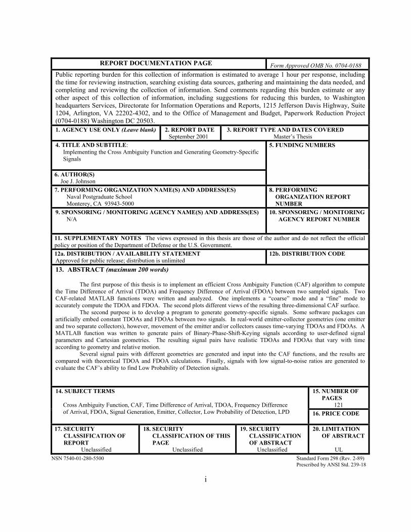
2. REPORT DATE September 2001

3. REPORT TYPE AND DATES COVERED Master’s Thesis

4. TITLE AND SUBTITLE: Implementing the Cross Ambiguity Function and Generating Geometry-Specific Signals

6. AUTHOR(S) Joe J. Johnson

5. FUNDING NUMBERS

7. PERFORMING ORGANIZATION NAME(S) AND ADDRESS(ES) Naval Postgraduate School Monterey, CA 93943-5000

8. PERFORMING ORGANIZATION REPORT NUMBER

9. SPONSORING / MONITORING AGENCY NAME(S) AND ADDRESS(ES) N/A

10. SPONSORING / MONITORING AGENCY REPORT NUMBER

11. SUPPLEMENTARY NOTES The views expressed in this thesis are those of the author and do not reflect the official policy or position of the Department of Defense or the U.S. Government. 12a. DISTRIBUTION / AVAILABILITY STATEMENT Approved for public release; distribution is unlimited

12b. DISTRIBUTION CODE

13. ABSTRACT (maximum 200 words)

The first purpose of this thesis is to implement an efficient Cross Ambiguity Function (CAF) algorithm to compute the Time Difference of Arrival (TDOA) and Frequency Difference of Arrival (FDOA) between two sampled signals. Two CAF-related MATLAB functions were written and analyzed. One implements a “coarse” mode and a “fine” mode to accurately compute the TDOA and FDOA. The second plots different views of the resulting three-dimensional CAF surface.

The second purpose is to develop a program to generate geometry-specific signals. Some software packages can artificially embed constant TDOAs and FDOAs between two signals. In real-world emitter-collector geometries (one emitter and two separate collectors), however, movement of the emitter and/or collectors causes time-varying TDOAs and FDOAs. A MATLAB function was written to generate pairs of Binary-Phase-Shift-Keying signals according to user-defined signal parameters and Cartesian geometries. The resulting signal pairs have realistic TDOAs and FDOAs that vary with time according to geometry and relative motion.

Several signal pairs with different geometries are generated and input into the CAF functions, and the results are compared with theoretical TDOA and FDOA calculations. Finally, signals with low signal-to-noise ratios are generated to evaluate the CAF’s ability to find Low Probability of Detection signals.

15. NUMBER OF PAGES 121

14. SUBJECT TERMS Cross Ambiguity Function, CAF, Time Difference of Arrival, TDOA, Frequency Difference of Arrival, FDOA, Signal Generation, Emitter, Collector, Low Probability of Detection, LPD 16. PRICE CODE

17. SECURITY CLASSIFICATION OF REPORT

Unclassified

18. SECURITY CLASSIFICATION OF THIS PAGE

Unclassified

19. SECURITY CLASSIFICATION OF ABSTRACT

Unclassified

20. LIMITATION OF ABSTRACT

UL

NSN 7540-01-280-5500 Standard Form 298 (Rev. 2-89) Prescribed by ANSI Std. 239-18

i

THIS PAGE INTENTIONALLY LEFT BLANK

ii

THIS PAGE INTENTIONALLY LEFT BLANK

iv

ABSTRACT The first purpose of this thesis is to implement an efficient Cross Ambiguity

Function (CAF) algorithm to compute the Time Difference of Arrival (TDOA) and

Frequency Difference of Arrival (FDOA) between two sampled signals. Two CAF-

related MATLAB functions were written and analyzed. One implements a “coarse”

mode and a “fine” mode to accurately compute the TDOA and FDOA. The second plots

different views of the resulting three-dimensional CAF surface.

The second purpose is to develop a program to generate geometry-specific

signals. Some software packages can artificially embed constant TDOAs and FDOAs

between two signals. In real-world emitter-collector geometries (one emitter and two

separate collectors), however, movement of the emitter and/or collectors causes time-

varying TDOAs and FDOAs. A MATLAB function was written to generate pairs of

Binary-Phase-Shift-Keying signals according to user-defined signal parameters and

Cartesian geometries. The resulting signal pairs have realistic TDOAs and FDOAs that

vary with time according to geometry and relative motion.

Several signal pairs with different geometries are generated and input into the

CAF functions, and the results are compared with theoretical TDOA and FDOA

calculations. Finally, signals with low signal-to-noise ratios are generated to evaluate the

CAF’s ability to find Low Probability of Detection signals.

v

THIS PAGE INTENTIONALLY LEFT BLANK

vi

TABLE OF CONTENTS

I. INTRODUCTION....................................................................................................... 1 A. BACKGROUND.............................................................................................. 1 B. OBJECTIVES.................................................................................................. 1 C. RELATED WORK ......................................................................................... 2 D. THESIS ORGANIZATION ........................................................................... 3

II. THE CROSS AMBIGUITY FUNCTION................................................................. 5 A. DEFINITION................................................................................................... 5 B. ANALYTIC SIGNAL VS. COMPLEX ENVELOPE.................................. 6

III. IMPLEMENTING THE CROSS AMBIGUITY FUNCTION ............................. 11 A. COMPUTATIONAL COMPLEXITY (COST) ANALYSIS .................... 11

1. The Fast Fourier Transform Method.............................................. 11 2. The Cross-Correlation Method........................................................ 13 3. The Summation Method ................................................................... 15

B. ANALYSIS OF CAF SOFTWARE............................................................. 17 1. The Coarse Mode .............................................................................. 17 2. The Fine Mode................................................................................... 20 3. The “CAF.m” Program .................................................................... 21 4. The “CAF_peak.m” Program .......................................................... 27

C. EXAMPLES AND RESULTS...................................................................... 28 1. Constant TDOA With Zero FDOA.................................................. 29 2. Constant TDOA and Constant FDOA ............................................ 34

IV. GEOMETRY-SPECIFIC SIGNAL GENERATION ............................................ 41 A. BINARY-PHASE-SHIFT-KEYING SIGNALS......................................... 41 B. EMITTER – COLLECTOR GEOMETRY................................................ 43 C. CALCULATING THEORETICAL TDOA(S) AND FDOA(S)................ 44

V. IMPLEMENTING THE SIGNAL GENERATOR................................................ 49 A. ANALYSIS OF THE SIGNAL GENERATION SOFTWARE ................ 49

1. The “Sig_gen.m” Program ............................................................... 49 2. The “Tdoa_fdoa.m” Program .......................................................... 55

B. EXAMPLE GEOMETRIES AND SIGNAL SETS.................................... 56 1. Constant TDOA and Zero FDOA.................................................... 56 2. Time-Varying TDOA and Constant FDOA.................................... 59 3. Time-Varying TDOA and Time-Varying FDOA ........................... 62 4. Simulated Low Earth Orbit Satellite Collectors ............................ 65 5. Simulated Airborne Collectors ........................................................ 68

C. USING THE CAF FOR SIGNAL DETECTION....................................... 71

VI. CONCLUSIONS........................................................................................................ 77 A. SUMMARY OF FINDINGS ........................................................................ 77 B. FUTURE WORK .......................................................................................... 77

vii

APPENDIX A: MATLAB CODE – CAF SOFTWARE................................................... 79 A. “CAF.M”........................................................................................................ 79 B. “CAF_PEAK.M”........................................................................................... 85 C. “SHIFTUD.M” .............................................................................................. 89

APPENDIX B: MATLAB CODE – SIGNAL GENERATION SOFTWARE ............... 91 A. “SIG_GEN.M”............................................................................................... 91 B. “TDOA_FDOA.M” ....................................................................................... 96

LIST OF REFERENCES ..................................................................................................... 99

INITIAL DISTRIBUTION LIST ...................................................................................... 101

viii

LIST OF FIGURES

Figure 2-1. Periodogram of a Sampled Bandpass Signal......................................................... 7 Figure 2-2. Periodogram of Analytic Signal. ........................................................................... 8 Figure 2-3. Periodogram of Complex Envelope. ..................................................................... 9 Figure 3-1. Coarse Mode Sub-Block Processing. .................................................................. 19 Figure 3-2. Flow Chart of Coarse Mode in CAF.m. .............................................................. 23 Figure 3-3. CAF.m Results – Case #1.................................................................................... 30 Figure 3-4. 3-D CAF Surface – Case #1. ............................................................................... 30 Figure 3-5. 2-D Cuts Through CAF Surface – Case #1. ........................................................ 31 Figure 3-6. CAF.m Results – Case #2.................................................................................... 32 Figure 3-7. 3-D CAF Surface – Case #2. ............................................................................... 32 Figure 3-8. 2-D Cuts Through CAF Surface – Case #2. ........................................................ 33 Figure 3-9. CAF.m Results – Case #3 (1st Iteration).............................................................. 35 Figure 3-10. CAF.m Results – Case #3 (2nd Iteration)........................................................... 35 Figure 3-11. CAF.m Results – Case #3 (3rd Iteration). .......................................................... 36 Figure 3-12. CAF.m Results – Case #3 (4th Iteration). .......................................................... 36 Figure 3-13. 3-D CAF Surface – Case #3. ............................................................................. 37 Figure 3-14. 2-D Cuts Through CAF Surface – Case #3. ...................................................... 37 Figure 3-15. CAF.m Results – Case #4.................................................................................. 38 Figure 3-16. 3-D CAF Surface – Case #4. ............................................................................. 39 Figure 3-17. 2-D Cuts Through CAF Surface – Case #4. ...................................................... 39 Figure 4-1. Example of a BPSK Signal (After [6])................................................................ 42 Figure 4-2. 2-D Emitter-Collector Geometry (After [7]). ...................................................... 44 Figure 5-1. Example Signal Set (Constant TDOA, FDOA = 0). ........................................... 57 Figure 5-2. CAF.m Results (Constant TDOA, FDOA = 0). .................................................. 58 Figure 5-3. 3-D CAF Surface (Constant TDOA, FDOA = 0)................................................ 58 Figure 5-4. 2-D Cuts Through CAF Surface (Constant TDOA, FDOA = 0)......................... 59 Figure 5-5. Example Signal Set (Time-Varying TDOA, Constant FDOA)........................... 60 Figure 5-6. CAF.m Results (Time-Varying TDOA, Constant FDOA).................................. 60 Figure 5-7. 3-D CAF Surface (Time-Varying TDOA, Constant FDOA). ............................. 61 Figure 5-8. 2-D Cuts Through CAF Surface (Time-Varying TDOA, Constant FDOA). ...... 62 Figure 5-9. Example Signal Set (Time-Varying TDOA and FDOA). ................................... 63 Figure 5-10. CAF.m Results (Time-Varying TDOA and FDOA). ........................................ 63 Figure 5-11. 3-D CAF Surface (Time-Varying TDOA and FDOA)...................................... 64 Figure 5-12. 2-D Cuts Through CAF Surface (Time-Varying TDOA and FDOA). ............. 64 Figure 5-13. Example Signal Set (LEO Satellite Collectors & Ground-Based Emitter). ...... 66 Figure 5-14. CAF.m Results (LEO Satellite Collectors & Ground-Based Emitter). ............. 66 Figure 5-15. 3-D CAF Surface (LEO Satellite Collectors & Ground-Based Emitter). ......... 67 Figure 5-16. 2-D Cuts Through CAF Surface (LEO Collectors & Ground Emitter)............. 67 Figure 5-17. Example Signal Set (Airborne Collectors & Ground-Based Emitter)............... 69 Figure 5-18. CAF.m Results (Airborne Collectors & Ground-Based Emitter). .................... 69 Figure 5-19. 3-D CAF Surface (Airborne Collectors & Ground-Based Emitter). ................. 70 Figure 5-20. 2-D Cuts Through CAF Surface (Airborne Collectors & Ground Emitter). ..... 70

ix

Figure 5-21. 2-D Cuts Through CAF Surface (LEO Collectors, Es/No = –20 dB). .............. 72 Figure 5-22. 2-D Cuts Through CAF Surface (LEO Collectors, Es/No = –40 dB). .............. 72 Figure 5-23. 2-D Cuts Through CAF Surface (LEO Collectors, Es/No = –45 dB). .............. 73 Figure 5-24. 2-D Cuts Through CAF Surface (LEO Collectors, Es/No = –50 dB). .............. 73 Figure 5-25. 2-D Cuts Through CAF Surface (LEO Collectors, Es/No = –55 dB). .............. 74

x

LIST OF TABLES

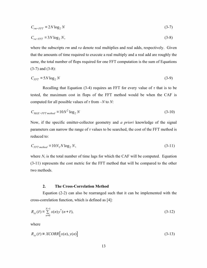
Table 3-1. Computational Complexities of Three Direct CAF Computation Methods. ........ 16

xi

THIS PAGE INTENTIONALLY LEFT BLANK

xii

ACKNOWLEDGMENTS

There are many people who helped make this thesis possible. I would first like to

thank the Professors at the Naval Postgraduate School who taught the numerous

Electrical Engineering classes that I took over the last two years. Their efforts took me

from the Computer Science Bachelor’s level to the Electrical Engineering Master’s level,

giving me all the tools along the way that I needed to complete my research and this

thesis. I am especially grateful to my advisor, Professor Herschel H. Loomis, Jr. His

patience and guidance got me through many rough spots during this whole process, and I

learned an enormous amount from him. Thank you, Professor. Thanks also to my

second reader, Professor Ralph D. Hippenstiel. He and his fine-toothed comb were

instrumental in improving the quality of this thesis.

Most importantly, I want to thank my wonderful wife, LCDR(sel) Holly M.

Johnson, CEC, USN, for her unfailing support throughout our two years in Monterey. I

am especially grateful for her strength in executing PCS orders to Washington, D.C.,

buying a home, and taking care of our kids, Alex and Kyra – all on her own while

performing full time Navy duties in outstanding fashion. She continues to amaze and

impress me. Thanks for everything, Honey. I love you.

xiii

THIS PAGE INTENTIONALLY LEFT BLANK

xiv

EXECUTIVE SUMMARY

The location of radio frequency transmitters is critical to numerous applications.

Many geolocation methods utilize the Time Difference of Arrival (TDOA) and

Frequency Difference of Arrival (FDOA) between two receivers collecting the same

transmission. One method of computing the TDOA and FDOA jointly is the Cross

Ambiguity Function (CAF). In the discrete, sampled-time case, it is defined

mathematically as:

1 2*1 2

0( , ) ( ) ( )

knN jN

nCAF k s n s n e

πτ

− −

== +∑ τ (1)

where and are sampled signals in analytic signal format, N is the total number of

samples in and , τ is time delay in samples, and

1s 2s

1s 2s kN

is the frequency difference in

digital frequency, or fraction of the sampling frequency. The magnitude of the CAF, or

( , kτ )CAF , will peak when τ and kN

are equal to the embedded TDOA and FDOA,

respectively, between the two signals and . The first goal of this thesis was to

implement Equation (1) to efficiently compute the TDOA and FDOA between two

sampled signals.

1s 2s

There are three main ways to implement Equation (1) directly. The summation

can be explicitly computed, or the terms can be rearranged in two different ways to force

Equation (1) into the form of either a Discrete Fourier Transform or a cross-correlation.

The three methods are evaluated and their computational complexities (in terms of

floating point operations) are compared. The result is that even for a relatively small

number of possible TDOAs and FDOAs, all three methods of direct computation are too

costly. A better approach is to split the computations into two modes: “coarse” and

“fine.” The coarse mode produces a rough estimation of TDOA and FDOA by dividing

the signals into smaller blocks for processing, which reduces the overall processing

burden. The coarse estimates are then sent to the fine mode for refined computation.

xv

Because the fine mode computes the CAF for a small number of possible TDOAs and

FDOAs (i.e., for a few values surrounding the coarse estimates), the CAF can be

implemented directly. From the analysis of the three methods described above, the

explicit summation method is the most efficient. This approach was used to develop a

MATLAB function, CAF.m, that takes two signal vectors and computes the associated

TDOA and FDOA. Another program, CAF_peak.m, displays the resulting CAF surface

in both 3-D and 2-D. Several pairs of signals with constant TDOAs and FDOAs were

input into the programs to ensure that they worked.

The second goal of the thesis was to develop a MATLAB program that generates

realistic signal sets. Some commercial software packages have the ability to embed only

constant TDOAs and FDOAs between two signals. In real-world systems, however, the

relative motion between emitters and collectors causes time-varying TDOAs and FDOAs.

The program sig_gen.m was developed so that a user can define signal parameters

(carrier frequency, sampling frequency, data rate, etc.) and a specific emitter-collector

geometry in Cartesian, three-dimensional, coordinates. The generated signal sets

represent realistic signals that have been transmitted from a system with the

characteristics defined by the user. In this manner, one can use sig_gen.m to simulate

real-world systems.

As an example, consider a ground-based transmitter with a pair of satellite

collectors in a Low Earth Orbit (LEO) of 1000 kilometers. Figure (1) shows the

MATLAB command window after sig_gen.m generates a pair of signals with this

geometry. The theoretical values for TDOA and FDOA are shown at the bottom of the

figure. Figure (2) shows the MATLAB command window after running CAF.m on the

generated signals. Notice that the computed values of TDOA and FDOA, shown in

Figure (2), compare favorably with the theoretical predictions in Figure (1). Finally,

Figure (3) shows the 3-D plot of the resulting CAF surface and Figure (4) shows 2-D

views that result from slices through the surface along the TDOA and FDOA axes. It is

important to note that the CAF surface is for display only, since its peak occurs at un-

interpolated values of TDOA and FDOA. This reduces the processing burden of creating

xvi

Figure 1. Example Signal Set (LEO Satellite Collectors & Ground-Based Emitter).

xviiFigure 2. CAF.m Results (LEO Satellite Collectors & Ground-Based Emitter).

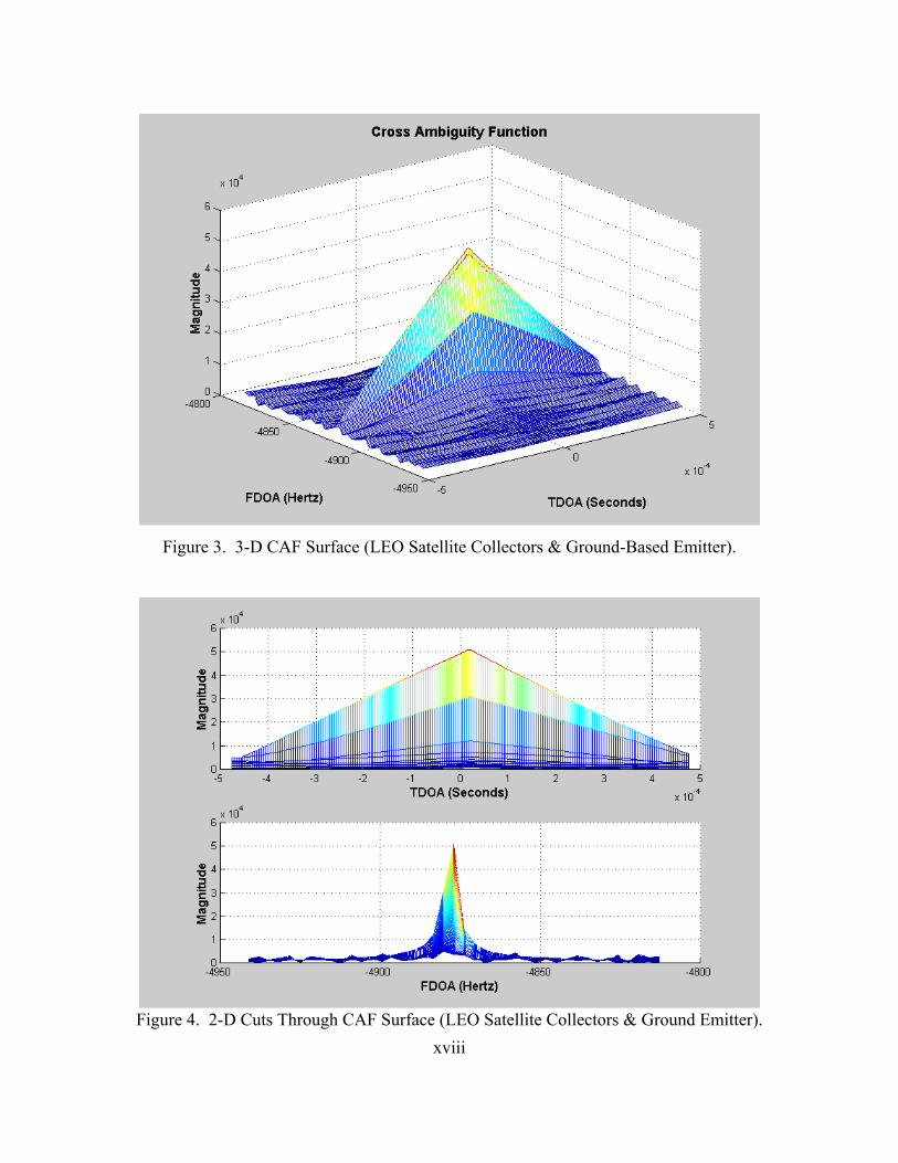
Figure 3. 3-D CAF Surface (LEO Satellite Collectors & Ground-Based Emitter).

Figure 4. 2-D Cuts Through CAF Surface (LEO Satellite Collectors & Ground Emitter).

xviii

the surface. As a result, the TDOA & FDOA shown in Figures (3) and (4) do not

correspond exactly to the more precise values computed by CAF.m and displayed in

Figure (2).

A variety of other signal sets were also generated to ensure that the programs

developed for this thesis operated correctly. The end result is that the goals of the thesis

were clearly met. The CAF and signal generation software developed for this thesis

provide a new capability for users to simulate real-world systems, generate realistic

BPSK signals, and efficiently compute TDOAs and FDOAs – all on a standard desktop

PC.

xix

THIS PAGE INTENTIONALLY LEFT BLANK

xx

I. INTRODUCTION Equation Section 1

A. BACKGROUND

Accurate geolocation of radio frequency transmitters is critical to many

applications, including Global Positioning and pinpointing the locations of hostile radar

systems. Many geolocation methods utilize the Time Difference of Arrival (TDOA) and

Frequency Difference of Arrival (FDOA) between two receivers collecting the same

transmission. If there is no FDOA between two receivers (i.e., the difference in the two

Dopplers is zero), then simple cross-correlation computations can uncover the resulting

TDOA. However, in the more likely cases where relative motion exists between

collectors and transmitters, the non-zero FDOAs preclude use of cross-correlation

techniques. In these cases, TDOA and FDOA measurements must be calculated jointly.

One way to accomplish this is to utilize the Cross Ambiguity Function (CAF).

There exist many signal generation software packages that can produce myriad

signal types (Phase Shift Keying, Amplitude Shift Keying, etc.) with user-defined

parameters such as carrier frequency, sampling frequency, symbol rate, and signal-to-

noise ratio. Some of these packages can also embed time delays and frequency offsets

between two signals. The limitation in these programs is that the embedded TDOAs and

FDOAs are constant. This is not helpful in modeling real-world situations where relative

motion between emitters and collectors causes a continuous change in geometry, and

therefore leads to TDOAs and FDOAs that are time-varying.

B. OBJECTIVES

1

The main objective of this thesis was to develop the MATLAB code in Appendix

A, which takes two sampled signals (i.e., transmissions from a single emitter received by

two separate collectors) and estimates the associated TDOA and FDOA using CAF

computations. In addition to TDOA and FDOA estimation, the CAF can also be used to

detect signals. This feature is useful in evaluating the effectiveness of so-called Low

Probability of Dectection (LPD) signals. The CAF is used in many real-world systems

that have vast computer resources with which to do the computations. This software,

however, brings the ability to perform CAF computations to the standard desktop PC.

The secondary focus of this thesis was to develop the MATLAB code in

Appendix B, which generates pairs of sampled signals based upon signal parameters and

emitter-collector geometries defined by the user. This will allow users to model any real-

world system by creating signal sets that could be transmitted and collected by emitters

and collectors in an associated geometry.

C. RELATED WORK There exist numerous technical papers and articles on the CAF, and on algorithms

that can be used to compute it. The vast majority of these papers refer back to [1], which

is generally regarded as the seminal work on CAF processing techniques. Stein’s paper,

along with many others, describes an algorithm for efficient computation of the CAF. A

significant search for references that deal specifically with implementing CAF algorithms

turned up nothing. Searching the worldwide web for CAF programs uncovered a short

MATLAB function that is part of a collection of free programs called the Time

Frequency Toolbox for MATLAB [2]. Analysis of that CAF program, however, showed

that it was rudimentary and incapable of processing signals that had greater than about

256 data elements. The CAF programs created as part of this thesis (Appendix A) are

capable of handling signals with as many as 524,288 elements. The main program

computes the CAF using the coarse mode algorithm described in [1], and a fine mode

algorithm that was selected based upon an analysis of computational complexity.

As far as geometry-specific signal generation is concerned, there appeared to be

no body of knowledge from which to draw upon. As mentioned in the previous section,

there are some commercial software packages, including one from Statistical Signal

Processing, Inc., that can embed constant TDOAs and FDOAs between two signals. The

signal generation software developed for this thesis (Appendix B), however, allows a user

to generate signals whose TDOAs and FDOAs, be they constant or time-varying, are

consistent with the defined parameters and emitter-collector geometries. The algorithm

used to generate these signals was developed and implemented through extensive trial

and error by the author and his thesis advisor.

2

D. THESIS ORGANIZATION The chapters of this thesis devoted to the CAF are organized as follows: Chapter

II provides background information about the CAF, including basic definitions and

requirements of the CAF’s input signals. Chapter III evaluates the computational

complexity (or cost) of three different ways in which the basic CAF can be directly

implemented. Also, the code in Appendix A is thoroughly analyzed to describe the

specific approach taken to implement the CAF. Finally, graphical and numerical results

are displayed and discussed for several example signal sets that were input into the

Appendix A programs.

There are two chapters devoted to geometry-specific signal generation. Chapter

IV provides background information about Binary-Phase-Shift-Keying (BPSK) signals

and the type of emitter-collector geometry that is modeled by the code. Also, equations

that can be used to manually calculate TDOAs and FDOAs for known emitter-collector

geometries are presented. Chapter V describes in detail the code in Appendix B,

analyzing the technique used to create the signal sets. Also, several example sets of

signals are generated, with their theoretical TDOAs and FDOAs calculated and compared

to the actual values computed by the CAF code in Appendix A. Various cases are

explored, including geometries that give different combinations of constant and time-

varying TDOAs and FDOAs. Also, signal sets from some realistic geometries (e.g.,

satellite and airborne collectors) are analyzed and displayed. Finally, the detectability of

LPD emitters is explored by showing how CAF results are affected by increasing the

noise level. Chapter VI summarizes the findings of this thesis, and also discusses a

number of extensions to this research that could be taken on by future students.

3

THIS PAGE INTENTIONALLY LEFT BLANK

4

II. THE CROSS AMBIGUITY FUNCTION Equation Section (Next)

A. DEFINITION

In [1], the Cross Ambiguity Function (CAF) is mathematically defined as:

* 21 2

0( , ) ( ) ( ) ,

Tj ftCAF f s t s t e dtπτ τ −= +∫ (2-1)

where and are continuous-time signals in analytic signal format (as defined in

section B below), T is the integration period in seconds, τ is time delay in seconds, and f

is the frequency offset in Hertz.

1s 2s

In order to shift Equation (2-1) into the discrete (or sampled) time domain, let t =

nTs and skffN

= , where Ts is the sample period, 1s

sf

T= is the sampling frequency, n

represents individual sample numbers, and N is the total number of samples. Inserting

these values back into Equation (2-1) and simplifying yields the discrete form of the

CAF:

1 2*1 2

0( , ) ( ) ( ) ,

knN jN

nCAF k s n s n e

πτ τ

− −

== +∑ (2-2)

where and are sampled signals in analytic signal form, N is the total number of

samples in and , τ is time delay in samples, and

1s 2s

1s 2s kN

is the frequency difference in

digital frequency, or fraction of the sampling frequency. The magnitude of the CAF, or

( , kτ )CAF , will peak when τ and kN

s

are equal to the embedded TDOA and FDOA,

respectively, between the two signals and . Note the assumption that the signal’s

presence has been previously detected, and subsequently collected as and . The

CAF itself is also capable of signal detection. This is discussed further in section V.C.

1 2s

1s 2s

The code in Appendix A was developed to efficiently implement Equation (2-2).

As will be shown in the next chapter, there are several different ways to implement

Equation (2-2). Efficiency becomes a large factor because of the potentially huge range

5

of TDOAs and FDOAs that must be searched. Equation (2-2) can uncover TDOAs in the

range –N to N and FDOAs for k in the range 2N− + 1 to

2N . To search the entire range

of possible TDOAs and FDOAs would require 2 calculations of the CAF, an ominous

task for large N!

2N

B. ANALYTIC SIGNAL VS. COMPLEX ENVELOPE

In [1], Stein presents Equation (2-1) and then notes that the input signals and

must be in complex envelope format. In actuality, the signals must be in analytic

signal format. This is clearly an issue of semantics, but since a significant amount of

time was lost attempting to compute the CAF on signals in complex envelope format, it is

worthwhile to present the difference between complex envelope and analytic signal.

1s

2s

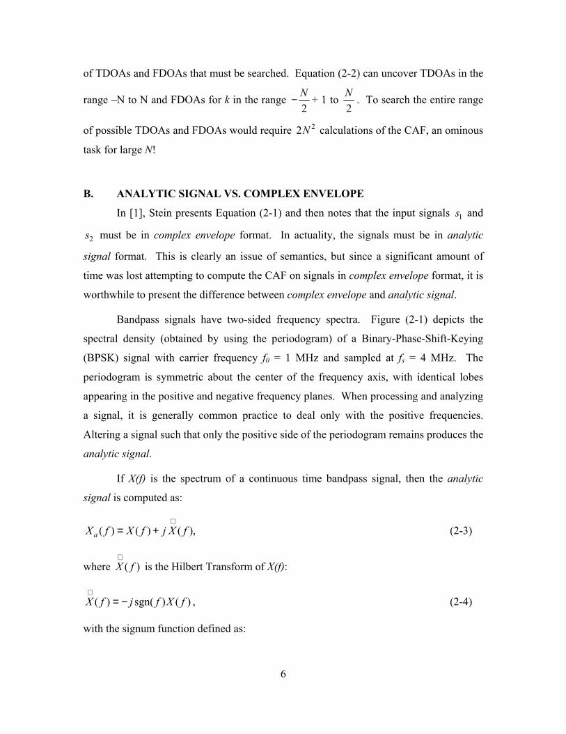
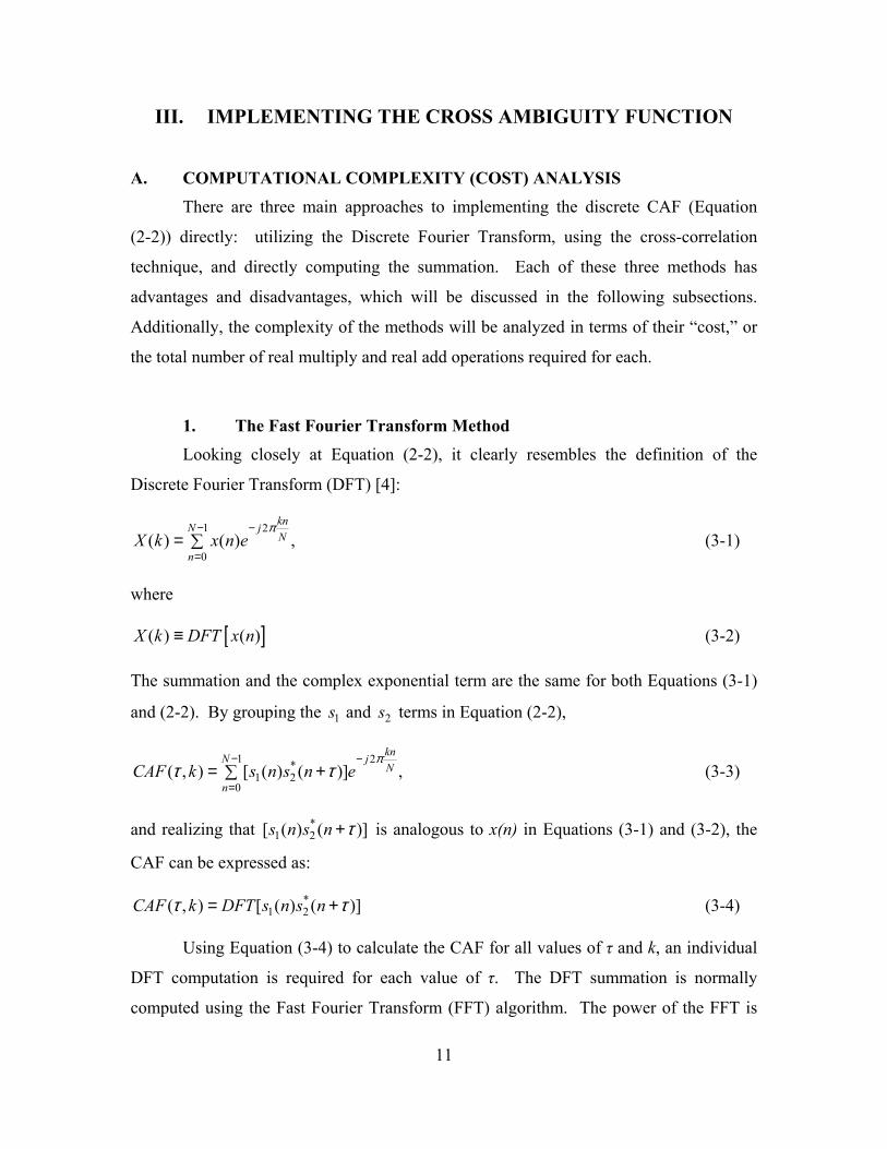
Bandpass signals have two-sided frequency spectra. Figure (2-1) depicts the

spectral density (obtained by using the periodogram) of a Binary-Phase-Shift-Keying

(BPSK) signal with carrier frequency f0 = 1 MHz and sampled at fs = 4 MHz. The

periodogram is symmetric about the center of the frequency axis, with identical lobes

appearing in the positive and negative frequency planes. When processing and analyzing

a signal, it is generally common practice to deal only with the positive frequencies.

Altering a signal such that only the positive side of the periodogram remains produces the

analytic signal.

If X(f) is the spectrum of a continuous time bandpass signal, then the analytic

signal is computed as:

( ) ( ) ( ),aX f X f j X f∧

= + (2-3)

where ( )X f∧

is the Hilbert Transform of X(f):

( ) sgn( ) ( )X f j f X∧

= − f , (2-4)

with the signum function defined as:

6

-2 -1.5 -1 -0.5 0 0.5 1 1.5 2

x 106

0

200

400

600

800

1000

1200

1400

1600

1800X(f) -- Periodogram of a Bandpass Signal

Frequency (Hz )

Mag

nitu

de o

f X(f)

Figure 2-1. Periodogram of a Sampled Bandpass Signal.

1, 0sgn( )

1, 0f

ff

+ >= − <

(2-5)

Substituting Equation (2-4) into Equation (2-3) and simplifying leads to [3]:

2 ( ), 0( )

0, 0aX f f

X ff

>= <

(2-6)

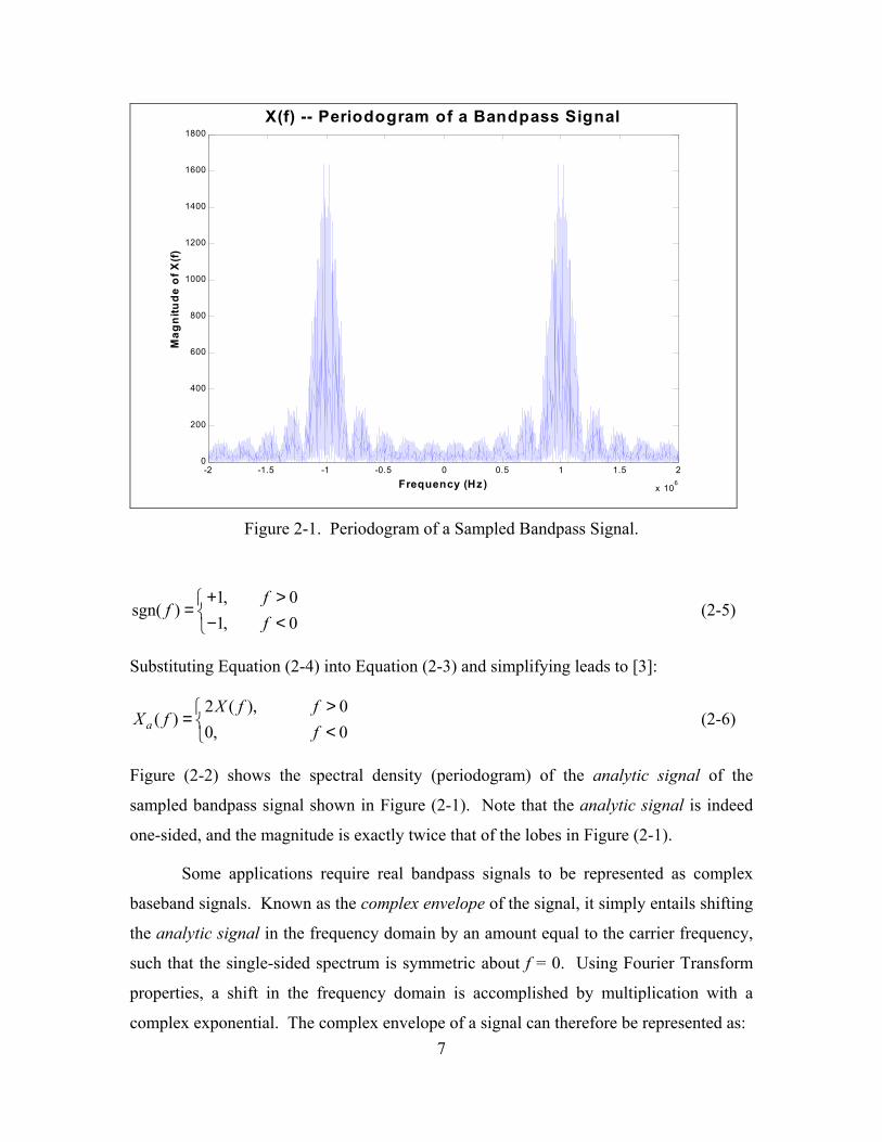
Figure (2-2) shows the spectral density (periodogram) of the analytic signal of the

sampled bandpass signal shown in Figure (2-1). Note that the analytic signal is indeed

one-sided, and the magnitude is exactly twice that of the lobes in Figure (2-1).

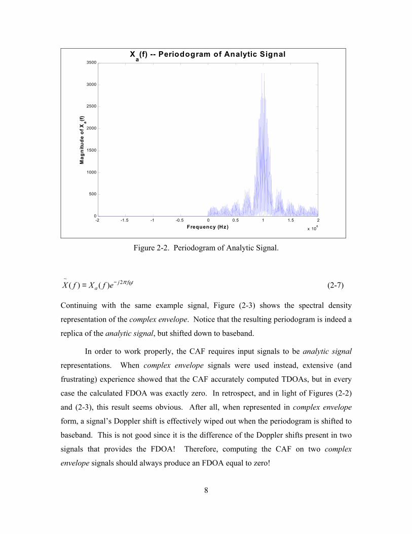
Some applications require real bandpass signals to be represented as complex

baseband signals. Known as the complex envelope of the signal, it simply entails shifting

the analytic signal in the frequency domain by an amount equal to the carrier frequency,

such that the single-sided spectrum is symmetric about f = 0. Using Fourier Transform

properties, a shift in the frequency domain is accomplished by multiplication with a

complex exponential. The complex envelope of a signal can therefore be represented as: 7

-2 -1.5 -1 -0.5 0 0.5 1 1.5 2

x 106

0

500

1000

1500

2000

2500

3000

3500X

a(f) -- Periodogram of Analytic Signal

Frequency (Hz)

Mag

nitu

de o

f Xa(f)

Figure 2-2. Periodogram of Analytic Signal.

~2 0( ) ( ) j f

aX f X f e π−= t (2-7)

Continuing with the same example signal, Figure (2-3) shows the spectral density

representation of the complex envelope. Notice that the resulting periodogram is indeed a

replica of the analytic signal, but shifted down to baseband.

In order to work properly, the CAF requires input signals to be analytic signal

representations. When complex envelope signals were used instead, extensive (and

frustrating) experience showed that the CAF accurately computed TDOAs, but in every

case the calculated FDOA was exactly zero. In retrospect, and in light of Figures (2-2)

and (2-3), this result seems obvious. After all, when represented in complex envelope

form, a signal’s Doppler shift is effectively wiped out when the periodogram is shifted to

baseband. This is not good since it is the difference of the Doppler shifts present in two

signals that provides the FDOA! Therefore, computing the CAF on two complex

envelope signals should always produce an FDOA equal to zero!

8

-2 -1.5 -1 -0.5 0 0.5 1 1.5 2

x 106

0

500

1000

1500

2000

2500

3000

3500Periodogram of Complex Envelope

Frequency (Hz)

Mag

nitu

de o

f Spe

ctru

m

Figure 2-3. Periodogram of Complex Envelope.

Now that the CAF has been mathematically defined, Chapter III will analyze the

computational complexity of three different methods that can be used to implement

Equation (2-2) directly. Chapter III will also describe in detail the actual approach used

by the MATLAB code in Appendix A to compute the CAF. Finally, Chapter III will

summarize the results of running the code on some example signal sets.

9

THIS PAGE INTENTIONALLY LEFT BLANK

10

III. IMPLEMENTING THE CROSS AMBIGUITY FUNCTION Equation Section (Next)

A. COMPUTATIONAL COMPLEXITY (COST) ANALYSIS

There are three main approaches to implementing the discrete CAF (Equation

(2-2)) directly: utilizing the Discrete Fourier Transform, using the cross-correlation

technique, and directly computing the summation. Each of these three methods has

advantages and disadvantages, which will be discussed in the following subsections.

Additionally, the complexity of the methods will be analyzed in terms of their “cost,” or

the total number of real multiply and real add operations required for each.

1. The Fast Fourier Transform Method Looking closely at Equation (2-2), it clearly resembles the definition of the

Discrete Fourier Transform (DFT) [4]:

1 2

0( ) ( ) ,

knN jN

nX k x n e

π− −

== ∑ (3-1)

where

[ ]( ) ( )X k DFT x n≡ (3-2)

The summation and the complex exponential term are the same for both Equations (3-1)

and (2-2). By grouping the and terms in Equation (2-2), 1s 2s

1 2*1 2

0( , ) [ ( ) ( )] ,

knN jN

nCAF k s n s n e

πτ τ

− −

== +∑ (3-3)

and realizing that [ ( is analogous to x(n) in Equations (3-1) and (3-2), the

CAF can be expressed as:

*1 2) ( )]s n s n τ+

*1 2( , ) [ ( ) ( )]CAF k DFT s n s nτ = τ+ (3-4)

Using Equation (3-4) to calculate the CAF for all values of τ and k, an individual

DFT computation is required for each value of τ. The DFT summation is normally

computed using the Fast Fourier Transform (FFT) algorithm. The power of the FFT is

11

that, for a given value of τ, it efficiently calculates the values associated with every value

of k (i.e., all digital frequencies). Since k can take on values from 2N− + 1 to

2N , the

complete range of digital frequencies kN

over which the FFT is calculated is

approximately

12

− to 12

. The main disadvantage with the FFT method is that for the

vast majority of emitter-collector geometry and signal parameter combinations, the

possible range of FDOAs is a very small subset of the full range of 12

− to 12

. Therefore,

the FFT method can waste valuable computer resources on unnecessary computations

when the FDOA search range is relatively small. Another disadvantage is the fact that

only integer values of k are evaluated in the FFT. In order to achieve higher resolution in

this method, the argument in Equation (3-4) could be padded with zeros before the FFT is

computed. This would effectively interpolate between integer values of k.

In order to compare the relative costs of the three methods, it is convenient to

evaluate the number of floating point operations (flops), i.e., multiplies and adds,

required for computation. In MATLAB, the “FFT” command is used to calculate the

DFT. From [5], the approximate number of complex multiplies and adds required for one

FFT (assumed to be radix-2 from here on) is

2log2cm FFTNC −

=

N

N

(3-5)

2log ,ca FFTC N− = (3-6)

where the subscripts cm and ca denote complex multiplies and complex adds,

respectively. Now, since complex numbers are of the form (X + jY), multiplying two of

them together requires four real multiplies (X1*X2, X1*Y2, Y1*X2, and Y1*Y2) plus two

real adds (one to sum the real terms and one to sum the imaginary terms). Adding two

complex numbers, on the other hand, requires just two real adds. Applying these two

relations to Equations (3-5) and (3-6) establishes the number of real multiplies and real

adds that occur during one FFT computation:

12

22 logrm FFTC N− = N

N

N

N

N

τ+

(3-7)

23 log ,ra FFTC N− = (3-8)

where the subscripts rm and ra denote real multiplies and real adds, respectively. Given

that the amounts of time required to execute a real multiply and a real add are roughly the

same, the total number of flops required for one FFT computation is the sum of Equations

(3-7) and (3-8):

25 logFFTC N= (3-9)

Recalling that Equation (3-4) requires an FFT for every value of τ that is to be

tested, the maximum cost in flops of the FFT method would be when the CAF is

computed for all possible values of τ from –N to N:

2210 logMAX FFT methodC N− = (3-10)

Now, if the specific emitter-collector geometry and a priori knowledge of the signal

parameters can narrow the range of τ values to be searched, the cost of the FFT method is

reduced to:

210 log ,FFT methodC N Nτ= (3-11)

where Nτ is the total number of time lags for which the CAF will be computed. Equation

(3-11) represents the cost metric for the FFT method that will be compared to the other

two methods.

2. The Cross-Correlation Method Equation (2-2) can also be rearranged such that it can be implemented with the

cross-correlation function, which is defined as [4]:

1 *

0( ) ( ) ( ),

Nxy

nR x n y nτ

−

== ∑ (3-12)

where

[ ]( ) ( ), ( )xyR XCORR x n y nτ ≡ (3-13)

13

The term “XCORR” is the MATLAB command that executes the cross-correlation

function. Equations (2-2) and (3-12) share a common summation term, so the terms in

the CAF expression must be rearranged and regrouped as follows:

*( )1 2 21 2

0( , ) ( ) ( ) ,

k n kN j jN N

nCAF k s n s n e e

τ τπ πτ τ

+− + −

=

= +∑

(3-14)

Note that the second, extra complex exponential is required in order to convert the n into

the (n + τ) term in the first complex exponential. Realizing that in Equation (3-14)

is analogous to x(n) in Equations (3-12) and (3-13), and that

1( )s n

( )2 22 ( )

k n kj jNs n e e

τ τπ πτ

++ − +

N is analogous to y(n + τ), the CAF can be expressed as:

( )21 2( , ) ( ), ( )

k njNCAF k XCORR s n s n e

τπτ

−+ =

(3-15)

Using Equation (3-15) to calculate the CAF for all values of τ and k, an individual

XCORR computation is required for each value of k. The power of the XCORR function

is that, for a given value of k, it calculates the values associated with every value of τ,

from –N to N. This can be very desirable compared to the FFT method since the probable

search range of TDOAs is likely to be much greater than the range of FDOAs that would

need to be searched. Another advantage to this method is that k does not have to be an

integer. In Equation (3-15), k can take on non-integer values, allowing for any desired

degree of resolution in FDOA calculation. The main disadvantage with the XCORR

method is that it is quite expensive since each invocation of XCORR requires more than

three times the number of flops as an FFT.

In order to analyze its cost, the XCORR function can be broken down into FFTs.

Note that the cross-correlation function, Equation (3-12) is essentially a convolution

without the time reversal in the y term. Convolutions, and thus cross-correlations, can be

computed efficiently by taking both signals into the frequency domain with FFTs,

multiplying the result, and then performing an inverse FFT to get back to the time

domain:

14

[ ] [ ]{ }1( ) * ( ) ( ) ( )xcorr

*x n y n FFT FFT x n FFT y n−≡ (3-16)

Therefore, every XCORR function requires three FFT operations (at a cost of three times

the number of flops listed in Equation (3-9)) plus N complex multiplies (or 6N flops) for

the element-by-element multiplication of the two inner FFTs in Equation (3-16). The

total number of flops required to compute a single XCORR function is therefore:

23*(5 log ) 6 3 (2 5log )XCORRC N N N N= + = + 2 N (3-17)

Now, assuming that k takes on the integer values in the range 2N− + 1 to

2N , the

maximum cost of the XCORR method would be approximately:

223 (2 5logMAX XCORR methodC N− = + )N

),N

(3-18)

In the likely event that geometry and signal parameters reduces the range of k values for

which the CAF needs to be calculated, the actual cost for the XCORR method would be:

(3-19) 23 (2 5logXCORR method kC N N= +

where Nk is the total number of frequency bins for which the CAF will be computed.

Equation (3-19) represents the cost metric for the XCORR method that will be compared

to the other two methods.

3. The Summation Method For this final method of computing the CAF, Equation (2-2) is calculated directly.

An advantage of the summation method is that it too can evaluate the CAF at any value

of k, allowing for high resolution FDOA calculations. The disadvantage is that it requires

a double loop to calculate the CAF for every value of τ and k. The reliance on loops is

very costly, particularly for interpretive programming languages such as MATLAB.

The maximum cost for the summation method would be for the case where the

CAF is computed for all 2N values of τ and all N values of k (assuming just the integer

values of k). Assuming that the cost of the conjugation operation is negligible, and that

the multiplies in the complex exponential are done ahead of time, each iteration of the

15

summation will require two complex multiplications, or 12 flops. Since the summation

goes through N iterations, the summation method’s maximum cost in flops is:

3*12*2 * 24MAX SUM methodC N N N− = N=

N N

(3-20)

Now, assuming that the range of τ and k values can be narrowed down, the actual cost of

the summation method would be:

(3-21) 12 ,SUM method kC Nτ=

where Nτ and Nk are the total numbers of τ and k values, respectively. Equation (3-21)

can be used to compare costs with the other two methods. Equations (3-11), (3-19), and

(3-21) can be used to evaluate which method would be most efficient for a particular

emitter-collector geometry and set of signal parameters, which of course would determine

the range of τ and k values (and thus Nτ and Nk) for which the CAF would need to be

evaluated.

Table (3-1) summarizes the maximum and narrowed search range complexities of

the three methods described above.

Method Maximum Complexity

(flops)

Narrowed Search Range

Complexity (flops)

FFT 2210 logN N 210 logN N Nτ

Cross-Correlation 223 (2 5logN N+ ) ) 23 (2 5logkN N N+

Summation 324N 12 kN N Nτ

Table 3-1. Computational Complexities of Three Direct CAF Computation Methods.

By comparing the maximum complexities in Table (3-1), if all possible integer

values of k and τ were to be searched, then the FFT method would be the most efficient.

If the range of τ and k values were narrowed by geometric and signal parameter

16

considerations, however, the most efficient method would depend upon the total number

of possible TDOAs and FDOAs, Nτ and Nk, that would be evaluated.

It is important to note that the three methods described represent direct

computations of the CAF. In most cases, Nτ and/or Nk would be large enough to make

“brute-force” computation of the CAF (using any of the three methods) an overwhelming

burden on computer resources. A more efficient approach involves a two-step

computation of the CAF, implementing a “coarse mode” and a “fine mode” to compute

the TDOA and FDOA within reasonable accuracy. [1] This is the approach implemented

by the MATLAB code in Appendix A. The following section describes the approach in

detail.

B. ANALYSIS OF CAF SOFTWARE As mentioned in the section above, the three methods of directly computing the

CAF are computationally much too expensive to use as a one-step process, even when the

number of τ and k values is narrowed due to knowledge of the specific geometry in use.

In order to reduce the processing burden to an acceptable level, computing the CAF can

be broken into two distinct parts: a “coarse” mode and a “fine” mode. In the coarse

mode, all possible values of τ and k (as determined by geometry and signal parameters)

are processed in order to produce a rough (or coarse) estimation of the TDOA and FDOA

between the two signals. The coarse estimates are then fed into the fine mode, which

computes the final TDOA and FDOA calculations. An algorithm for the coarse mode is

described in [1] and is the basis for the code generated for this thesis. As for the fine

mode, the summation method described in the previous section is used. The following

subsections describe the coarse and fine modes, as well as their implementation in

“CAF.m,” which is listed in Appendix A.

1. The Coarse Mode Reference [1] provides an algorithm to calculate coarse estimates of the TDOA

and FDOA between two signals. The goal of the algorithm is to produce coarse estimates

that are accurate enough to enter a fine mode, while keeping processing burden as small

17

as possible. In order to accomplish this, the algorithm makes use of convolution

properties, as well as breaking the input signals into smaller blocks to speed processing.

The algorithm is represented by the following modified version of Equation (2-2) [1]:

211 * 111 1 2

0( , ) ( ; ) ( ; ) 0,...,

2

kmjN NR

k

NCAF qN m v S k v R S k R q e mπ−−

=+ = + + =∑ (3-22)

In Equation (3-22), refers to the FFT of the Rth block of and

refers to the FFT of the Rth block of . As mentioned, and are

processed in sub-blocks that are smaller than the total number of data points in each

signal, N. The size of each sub-block is elements, q is an index for the sub-block(s)

being processed, and v represents the frequency bin shift. The notation

1( ; )S k R 1( )s n

2S2 ( ; )S k R 2 ( )s n 1S

1N

RCAF refers to

the calculation which combines the Rth block of with the (R + q)th block of . In

order to avoid circular convolution effects, 50 percent overlap is utilized, such that the

(R + q)th block of S consists of

1S 2S

21

2N data elements and 1

2N zeros. Recalling Equation

(3-4), Equation (3-22) can be rewritten as:

*1 1 2( , ) ( ; ) ( ;RCAF qN m v DFT S k v R S k R q+ = + + ) (3-23)

Equation (3-23) calculates RCAF for all values of m (from 0 to 1

2N ) for a given q

and v. For every fixed combination of q and v, RCAF is computed for each sub-block

(i.e., for R = 1 to 1

NN

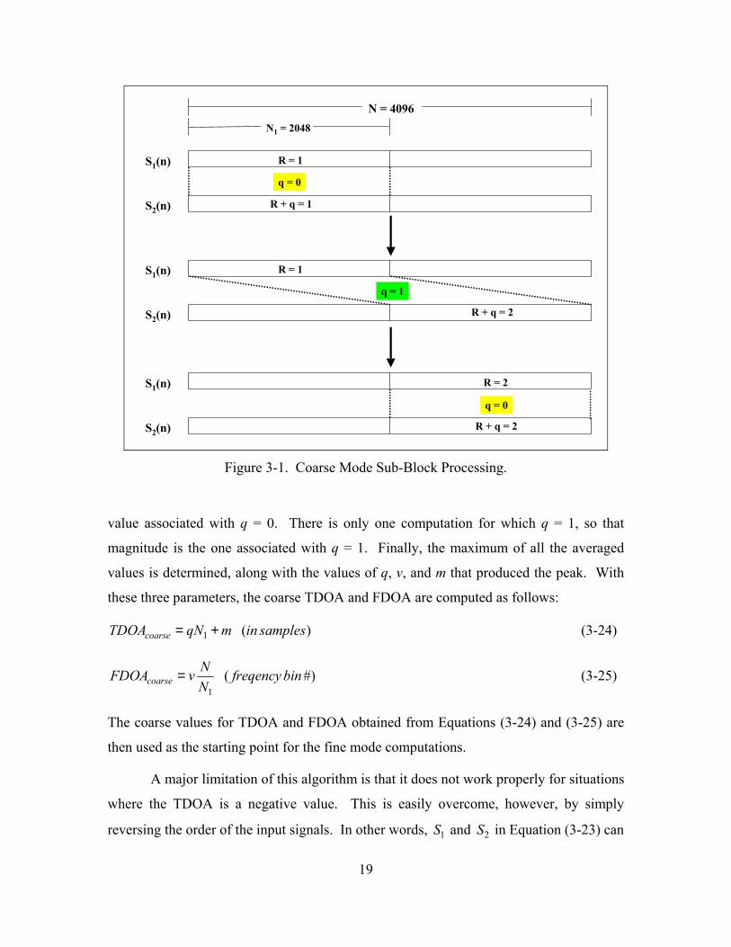
). Figure (3-1) illustrates how the sub-blocks would be processed

for two signals of length N = 4096 and a sub-block length of N1 = 2048. For R = 1, the

first block of is processed with the first and second blocks of (q goes from 0 to 1,

making (R + q) go from 1 to 2). For R = 2, the second block of is processed only with

the second block of sub-block (in this case, q cannot exceed 0 since (R + q) cannot

exceed the total number of sub-blocks). The magnitudes of the calculations are then

averaged to obtain one value for every fixed q and v. For example, in Figure (3-1), there

are two computations for which q = 0. These two magnitudes are averaged to get the

1S 2S

1S

2S

18

N = 4096N1 = 2048

R = 1

q = 0

S1(n)

S2(n) R + q = 1

R = 1

q = 1

S1(n)

S2(n) R + q = 2

R = 2

q = 0

S1(n)

S2(n) R + q = 2

Figure 3-1. Coarse Mode Sub-Block Processing.

value associated with q = 0. There is only one computation for which q = 1, so that

magnitude is the one associated with q = 1. Finally, the maximum of all the averaged

values is determined, along with the values of q, v, and m that produced the peak. With

these three parameters, the coarse TDOA and FDOA are computed as follows:

1 (coarseTDOA qN m in samples= + ) (3-24)

1(coarse

NFDOA v freqency binN

= #) (3-25)

The coarse values for TDOA and FDOA obtained from Equations (3-24) and (3-25) are

then used as the starting point for the fine mode computations.

A major limitation of this algorithm is that it does not work properly for situations

where the TDOA is a negative value. This is easily overcome, however, by simply

reversing the order of the input signals. In other words, and in Equation (3-23) can 1S 2S

19

be switched if necessary to avoid a negative TDOA. The only effect on TDOA and

FDOA when reversing the order of the signals is that the sign is flipped in both cases.

Unlike the case for negative TDOAs, the algorithm works fine for both positive and

negative FDOAs.

2. The Fine Mode Once coarse estimates of the TDOA and FDOA have been computed by finding

the maximum value of the CAF, it is necessary to interpolate that peak in order to obtain

the actual TDOA and FDOA within the desired resolution. This is what the fine mode

accomplishes. Since the fine mode need only evaluate a few TDOAs and FDOAs on

either side of the coarse estimates, one of the three direct computation methods described

in section A above can be utilized without much burden on processing resources.

In order to determine which of the three methods is most efficient for fine mode

calculations, it is convenient to compare the “Narrowed Search Range” computational

complexity equations summarized in Table (3-1). Since Nτ and Nk will be relatively small

in the fine mode, it is clear that the FFT method will be more efficient than the cross-

correlation method. So, to decide which method to use, the FFT and summation

equations can be compared as follows:

212 10 logkN N N N N Nτ τ< (3-26)

Canceling like terms and simplifying yields:

25 log6kN < N (3-27)

or

1.22 NkN > (3-28)

If Inequalities (3-27) and (3-28) are true, then the summation method is the one to use.

Otherwise, the FFT method would be the most efficient. It is a fair assumption that

will not be more than 10 for fine mode calculations. Therefore, the summation

method would be the most efficient method when . For coding

kN

1.2(10)2 4096N or N> >

20

purposes, the assumption was made that sampled signals used in the CAF would contain

more than 4096 elements. Therefore, the fine mode is accomplished by implementing the

summation method. The MATLAB program written to perform the coarse and fine

computations is called “CAF.m”. The next section describes it in detail.

3. The “CAF.m” Program The program CAF.m, listed in Appendix A, is a MATLAB function that

computes the TDOA and FDOA between two sampled signals. It is invoked in the

MATLAB command window with a line of the form:

[TDOA, FDOA] = CAF(S1, S2, Max_f, fs, Max_t);

The input arguments S1 and S2 are the two sampled signals in analytic signal format.

Max_f is the maximum magnitude of FDOA, in Hertz, that is expected between the two

signals. The argument fs is the sampling frequency used to generated the sampled signals

S1 and S2. The sampling frequency is assumed to be the same for both signals. Max_t is

the maximum TDOA, in seconds, expected. Note that Max_f and Max_t are functions of

the geometry and signal parameters for a given scenario. Also note that Max_t must be

positive do to the coarse mode algorithm’s constraint, as described in section 1 above. If

the expected Max_t is negative, then S1 and S2 need only be reversed in the function call

shown above (e.g., [TDOA, FDOA] = CAF(S2, S1, Max_f, fs, Max_t);). The output

arguments TDOA and FDOA make the computations available to the MATLAB user in

variables of the same names.

The first step in CAF.m is to reshape S1 and S2 to ensure that they are column

vectors. This takes advantage of the fact that MATLAB stores variables and performs

computations on them in a column-wise fashion. Next, the most appropriate size of sub-

block (N1) is determined. N1 nominally starts out at 1024, but the while loop ensures

that N1 is large enough to ensure proper resolution. For example, if the maximum

frequency bin expected _ 1Max f Nfs

were less than one, then the resolution would not

be good enough to discern the correct frequency bin. Until acceptable resolution is

obtained, N1 is successively multiplied by two. This takes advantage of MATLAB’s

21

more efficient FFT operations on vectors whos sizes are powers of two. In no case will

N1 be larger than 2 , as this is roughly the maximum size for which

processing is efficiently possible. Clearly this is dependent upon the specific system

being used for the processing. In some cases, the sub-block size may be larger than the

size (N) of the signal vectors. In this case, CAF.m will pad the signal vectors with

enough zeros to make the overall length equal to N1.

19 524288=

Next, CAF.m determines the total number of sub-blocks that are in the signal

vectors, Number_of_Blocks. This is simply 1

NN

, where N is the length of the signals and

N1 is the size of one sub-block. Every block of will be processed, so the variable R

will go from one to Number_of_Blocks. The program then uses the input arguments

Max_t and Max_f to determine the range of values for q and v, respectively, that must be

used in the subsequent calculations. Note that each sub-block represents a period of time

equal to

1S

1 sN T , and q represents multiples of this value. Therefore, q’s values will be

dependent upon how large the maximum expected TDOA (Max_t) is. For example, if

Max_t is three microseconds and 1 sN T is two microseconds, then q need only take on the

values zero, one, and two. Any value greater than two would cause unnecessary

processing since it would correspond to TDOAs above Max_t. Likewise, the frequency

bin values, v, that need to be computed are determined from the user’s defined Max_f.

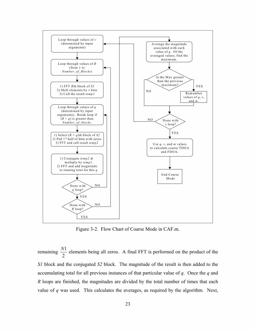
The heart of the coarse mode section of CAF.m is a triple nested loop, which runs

through all of the required values for R, q, and v. Figure (3-2) is a flow chart that shows

the triple loop and the processing steps that occur for the coarse mode. The outermost

loop runs through all of the required values of v. The next loop runs through all values of

R (i.e., from one to Number_of_Blocks). Within the R loop, the program picks out the

elements of S1 that correspond to the Rth block, and then performs an FFT on the result.

As required by Equation (3-23), the resulting FFT is then shifted by v frequency bins.

The innermost loop then runs through all required values of q. As per Equation (3-23),

the (R + q)th block of S2 is then obtained and subjected to an FFT. Note that, as required

by the algorithm, only the first 12

N data elements of the (R + q)th block are used, with the

22

Loop through values of v(determ ined by input

argum ents)

Loop through values of R(from 1 to

Num ber_of_Blocks)

1) FFT R th block of S12) Shift elem ents by v bins

3) Call the result temp1

Loop through values of q(determ ined by input

argum ents). B reak loop if (R + q) is greater than

Number_of_blocks.

1) Select (R + q)th block of S22) Pad 1st half of data w ith zeros

3) FFT and call result tem p2

1) Conjugate temp2 & m ultiply by temp1.

2) FFT and add m agnitudeto running total for this q .

Average the m agnitude associated with each

value of q . O f the averaged values, find the

m axim um .

Is the M ax greaterthan the previous

m axim um ?

Rem em bervalues of q , v ,

and m .

YESNO

Use q , v , and m valuesto calculate coarse TDOA

and FD OA.

End Coarse M ode

Done withq loop?

D one withR loop?

Done withv loop?

NO

NO

NO

YES

YES

YES

Figure 3-2. Flow Chart of Coarse Mode in CAF.m.

remaining 12

N elements being all zeros. A final FFT is performed on the product of the

S1 block and the conjugated S2 block. The magnitude of the result is then added to the

accumulating total for all previous instances of that particular value of q. Once the q and

R loops are finished, the magnitudes are divided by the total number of times that each

value of q was used. This calculates the averages, as required by the algorithm. Next,

23

the maximum value contained in the resulting matrix of values is compared to the current

max value. If it is greater, then the program saves that value, as well as the q, v, and m

that caused the new maximum. Once the v loop is completed, all computations have been

accomplished for the coarse mode, and the resulting values of q, v, and m are then used to

compute the coarse TDOA and FDOA using Equations (3-24) and (3-25), respectively.

Note that in Equation (3-24), m represents the frequency bin number of the N1-sized

FFT. In CAF.m, m is really the index into the FFT. In order to convert that index into

the actual frequency bin number, the term 1 12

N m− + + is used since the FFT elements

begin with the 1 12

N− + th frequency bin. So, to summarize, the

1 1

2N m− + +

term in

CAF.m is equivalent to m in Equation (3-24).

The next section of CAF.m represents the fine mode of the CAF computation.

Because the accuracy of the course estimations is not great, and because noise in the

input signals degrades the accuracy even further, the initial fine computations are made

for a fairly large number of parameter values. The set of time samples computed

(contained in the vector tau_val) is the coarse TDOA estimation plus or minus 10

samples. Likewise, the set of frequency bins computed (contained in the vector k_val) is

the coarse FDOA estimation plus or minus 10 bins.

Next, the summation method (Equation (2-2)) is used to carry out the fine

calculations. This requires a double loop to run through all of the values contained in the

k_val and tau_val vectors. For each value of k, the complex exponential term is

computed as a vector, so that N separate calculations are not required within the inner

loop. This reduces the overall processing burden. In the inner loop, the S2 vector (which

is already conjugated as required in Equation (2-2)) is shifted the appropriate number of

time samples. The shift operation is accomplished by the MATLAB function shiftud.m,

obtained from [9] and listed in Appendix A. Finally, the S1, S2, and exponents vectors

are multiplied (element by element in one step using MATLAB’s “.*” command) and

then summed to obtain one scalar value. The magnitude of that value is then stored in a

matrix for that particular value of k and t. Once the double loop is finished, the

maximum value in the CAF matrix is determined, along with the values of TDOA and 24

FDOA that caused that maximum value. The variables TDOA and FDOA then contain

the initial fine mode calculations.

The TDOA is displayed to the user in both samples and seconds, and the FDOA is

displayed in both digital frequency and Hertz. The user is also told to what resolution the

solutions are calcualated, in seconds for the TDOA and in Hertz for the FDOA. The user

is then given the following options:

1) Re-compute with finer resolution for TDOA

2) Re-compute with a finer resolution for FDOA

3) Re-compute with finer resolutions for both TDOA and FDOA

4) Keep the current solutions

The TDOA computation involves shifting the S2 vector a specific number of samples (or

elements). Since it is only possible to shift elements by an integer amount, the only way

to increase the TDOA resolution is to increase the sampling frequency of the signal

vectors. This follows from the fact that the TDOA in seconds is equal to the TDOA in

samples divided by the sampling frequency. A very quick way to increase the sampling

frequency of a vector in MATLAB is to use the built-in interp function, which will

resample a vector at a specified integer multiple of the original sampling frequency. The

resulting vector’s length is the specified integer times the original length, thereby

ensuring that the exact same period of time is covered in the new vector. In CAF.m, if

the user chooses to compute a TDOA with higher resolution, then S1 and S2 are

resampled at twice their sampling frequency, thereby increasing the TDOA resolution by

a factor of two. Now, for a fine TDOA computation, the true value will be within 0.5

samples on either side of the calculation. Therefore, successive TDOA computations

(i.e., after doubling the sampling frequency) need only check three possible TDOAs: the

previously calculated TDOA multiplied by two, plus the value on either side of it. For

example, if a TDOA is computed to be 18 samples, the true value would be somewhere

between 17.5 and 18.5 samples. Doubling the sampling frequency, the TDOAs to check

would be 18*2 ± 1, or sample numbers 35, 36, and 37.

25

The FDOA computation simply involves the value of k used in the complex

exponential term in Equation (2-2). As mentioned in section III.A.3 above, an advantage

of the summation method is that any value of k can be used; it is not restricted to integer

numbers. This makes increasing FDOA resolution quite easy. The approach used in

CAF.m is to increase the FDOA resolution by a factor of 10. For a fine FDOA

computation, the true value will be in the range of 0.5 10xk x± , where x is the exponent

when k is in scientific notation form. Taking 11 equally spaced values in that range will

provide a resolution improved by a factor of 10. For example, if a fine FDOA is

computed to be 0.6 ( 6 1 ) bins, the true value will be somewhere in the range

, or 0.55 to 0.65. Therefore, the FDOA would be recomputed by testing

the 11 values of k from 0.55 to 0.65, spaced 0.01 apart.

10x −

20.6 0.5 10x −±

The entire fine mode in CAF.m is enclosed in a while loop that continues to

perform more improved calculations of TDOA and/or FDOA until either: 1) the user is

satisfied with the results, or 2) the maximum processing capacity has been reached. In

the second case, TDOA improvement ends when the length of S1 and S2 reaches

. The FDOA can continue to be improved upon until the user is satisfied.

When processing capacity is reached, the options that include TDOA optimization

(numbers one and three in the list above) are removed from the user’s list of options.

Once the optimization is complete and a final TDOA and FDOA have been reached, the

user is given the option of displaying the actual CAF surface graphically. The CAF

surface is computed and plotted by the CAF_peak.m function, which is listed in

Appendix A, and described in the next section. The CAF surface is computed for the

original S1 and S2, in order to minimize processing burden. The surface is computed for

the TDOA ± 50 samples, and for the FDOA ± 20 frequency bins. It is important to note

that the CAF surface is for display only, as its peak occurs at un-interpolated values of

TDOA and FDOA. Once the surface is plotted, or if the user opts to not plot it, the

CAF.m function is completed. Section III.C below shows the results of running some

example signal sets through CAF.m.

192 524288=

26

4. The “CAF_peak.m” Program The program CAF_peak.m, listed in Appendix A, is a MATLAB function that

computes the CAF surface by comparing two sampled signals. It is invoked with a line

of the form:

[TDOA, FDOA, MaxAmb, Amb] =

CAF_peak(S1, S2, Tau_Lo, Tau_Hi, Freq_Lo, Freq_Hi, fs);

The input arguments S1 and S2 are the two sampled signal vectors in analytic signal

format. The arguments Tau_Lo and Tau_Hi represent the lowest and highest number of

samples for which to compute the CAF surface. Likewise, Freq_Lo and Freq_Hi

represent the lowest and highest digital frequencies for which to compute the CAF

surface. Finally, fs is the sampling frequency. The output arguments TDOA and FDOA

make the computations available to the MATLAB user in variables of the same names.

Note again that this program does not compute interpolated solutions of TDOA and

FDOA. It uses the FFT method described in section III.A.1 above. The TDOA’s

resolution is therefore only 0.5 samples, or 0.5 sT seconds. The FDOA’s resolution is

0.5N

(digital frequency), or 0.5sfN Hertz. The output arguments MaxAmb and Amb return

the magnitude of the surface’s peak and the matrix of values for the CAF surface (as

bounded by the input arguments), respectively.

The first section of CAF_peak.m performs a number of checks to ensure that the

input arguments are valid. These checks are not really necessary when CAF.m calls the

function, because CAF.m properly calculates the input arguments. But CAF_peak.m can

also be called directly by a user in the MATLAB command window. This is where the

checks become useful. The function checks to ensure that there are enough input

arguments, and that S1 and S2 are indeed vectors (and not matrices). The program then

reshapes the signal vectors to ensure that they are columns in order to take advantage of

MATLAB’s column-wise nature. The program uses zero padding to ensure that the

signals are of the same length, and that their length is a power of two (again, for

computing efficiency). Next, Tau_Lo and Tau_Hi are checked to ensure that they are

integers in the range –N to N and Freq_Lo and Freq_Hi are checked to ensure that they

27

are in the range –0.5 to 0.5. Finally, the program ensures that Tau_Lo and Freq_Lo are in

fact smaller than Tau_Hi and Freq_Hi, respectively.

Since the FFT method computes the CAF for all frequency values represented by

the bins 12Nk = − +

to

2N , the program must determine the indices into each FFT that

correspond to the user’s defined range of Freq_Lo to Freq_Hi. Next, the CAF is

computed in a for loop that runs through all of the values defined by the user’s range of

Tau_Lo to Tau_Hi. For each value, Equation (3-4) is computed by performing an FFT on

the product of S1 with the conjugated S2, which is shifted by an amount equal to the loop

variable t. The appropriate values are then extracted using the previously calculated

indices. The magnitude of the resulting vector is then placed as a new column in the Amb

matrix. When the loop is completed, Amb contains all values for the CAF surface, as

bounded by the input arguments. Furthermore, Amb’s rows represent frequency bins and

its columns represent numbers of samples. The maximum value of Amb is the peak of

the CAF surface, and the row and column associated with that peak are the FDOA and

TDOA, respectively. Finally, CAF_peak.m produces four different graphical views of

the CAF surface. The first is a three-dimensional view, the second is a two-dimensional

view looking at the TDOA axis, the third is a two-dimensional view along the FDOA

axis, and the final plot is a two-dimensional flat view looking down on the surface. The

next section shows the result of running some example signal sets through the CAF.m

and CAF_peak.m programs.

C. EXAMPLES AND RESULTS In order to test and evaluate the CAF.m and CAF_peak.m programs to ensure that

they performed accurate computations, signal pairs with known TDOAs and FDOAs

embedded in them were required. To aid in the testing and evaluation, a signal

generation software package from Statistical Signal Processing, Inc. (SSPI) [10] was used

to create signals with TDOAs and FDOAs. The SSPI software was capable of producing

only constant TDOAs and FDOAs, which caused no problem for testing and evaluation

purposes. But as discussed in Chapter I, constant TDOAs and FDOAs are not found in

real-world applications. Emitter-collector geometries change with time due to relative 28

motion between them, making the associated TDOAs and FDOAs themselves time-

varying. This issue is discussed further in Chapters IV and V.

To validate the accuracy of the CAF.m and CAF_peak.m programs, several

sampled signals with different time delays and frequency offsets were generated with

SSPI software. Several combinations of signals were input into CAF.m and

CAF_peak.m to ensure that their solutions matched the known TDOAs and FDOAs. The

following subsections detail the results.

1. Constant TDOA With Zero FDOA For Case #1, a pair of signals with the following parameters were input into the

CAF.m program:

Signal Type: BPSK with rectangular envelope

Carrier Frequency: 0.21 (digital frequency)

Samples Per Bit: 16

Signal-to-Noise Ratio for the two signals: 20 dB & 20 dB

Number of Samples: 65536

TDOA: 358 samples

FDOA: 0 (digital frequency)

Note that digital frequency is used and no specific sampling frequency is defined. For

testing purposes, however, a sampling frequency of fs = 1 MHz was assumed. This

makes the effective symbol rate 1 62,50016 /

MHz bpssamples bit

= . The expected TDOA is

then 46

358 358 3.58 101 10s

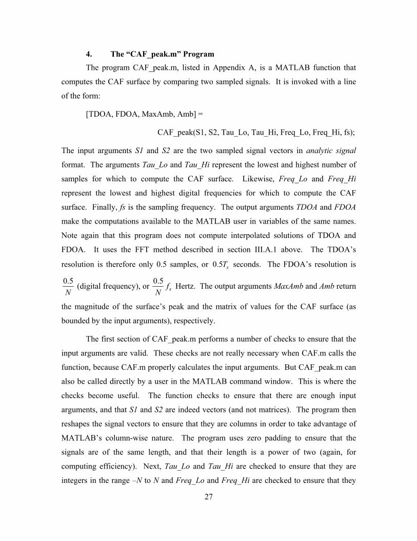
samples xf x

−= = seconds. The expected FDOA is 0 * fs = 0 Hz.

Figure (3-3) shows the MATLAB command window with the results of running CAF.m

on the signal pair described above. Note that because the signals were generated with

zero FDOA and an integer number of samples for TDOA, CAF.m’s first computation

29

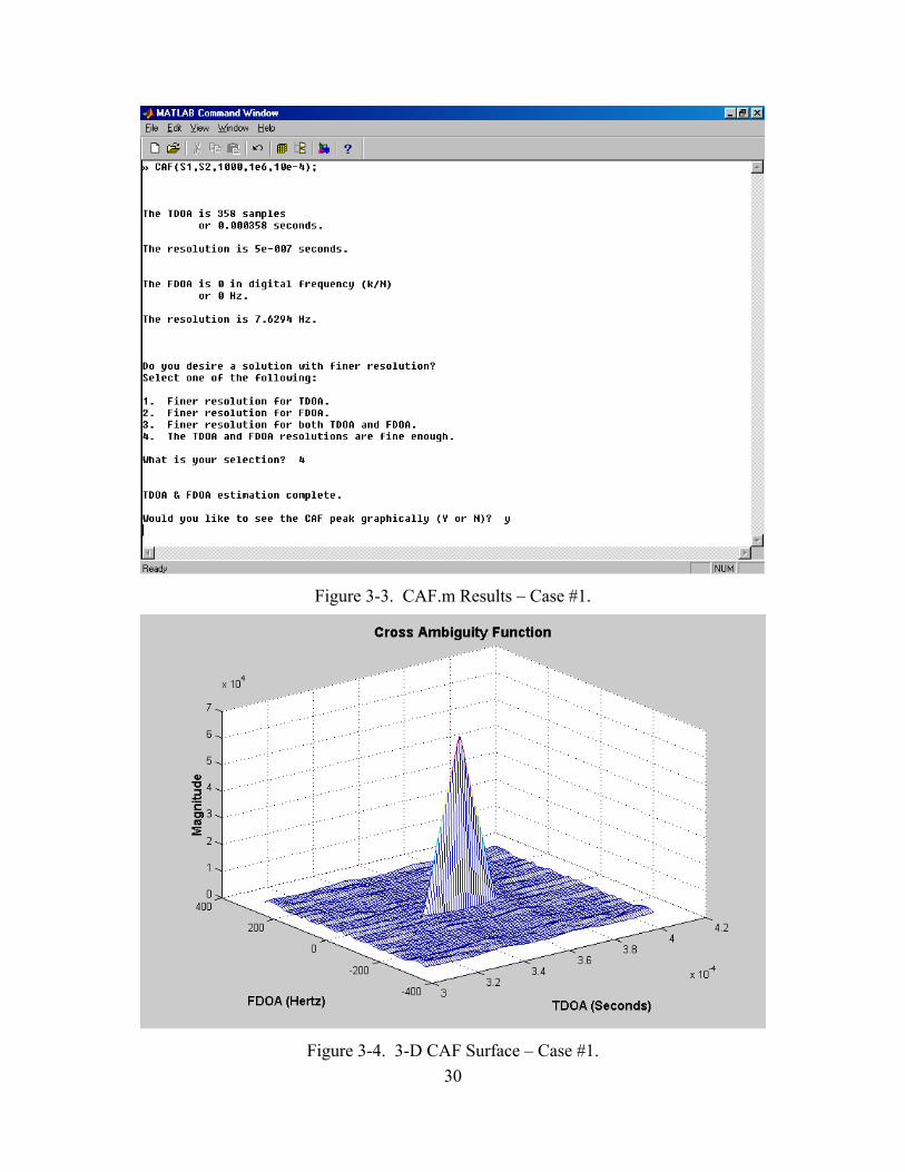
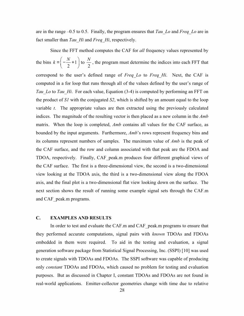
Figure 3-3. CAF.m Results – Case #1.

Figure 3-4. 3-D CAF Surface – Case #1.

30

Figure 3-5. 2-D Cuts Through CAF Surface – Case #1.

produces the exact solution. Therefore, no further iterations of the fine mode were

required. Figure (3-4) shows a three-dimensional view of the CAF surface, while Figure

(3-5) provides two-dimensional slices of the surface along the TDOA and FDOA axes.

Note the triangular shape of the surface along the TDOA axis. This makes sense

considering that the basic CAF equation is in the form of a convolution summation.

When two rectangular-envelope pulses are convolved, the result is triangular.

For Case #2, a pair of signals with the following parameters were input into the

CAF.m program:

Signal Type: BPSK with half-cosine envelope

Carrier Frequency: 0.21 (digital frequency)

Samples Per Bit: 16

Signal-to-Noise Ratio for the two signals: 0 dB & -20 dB

Number of Samples: 65536

31

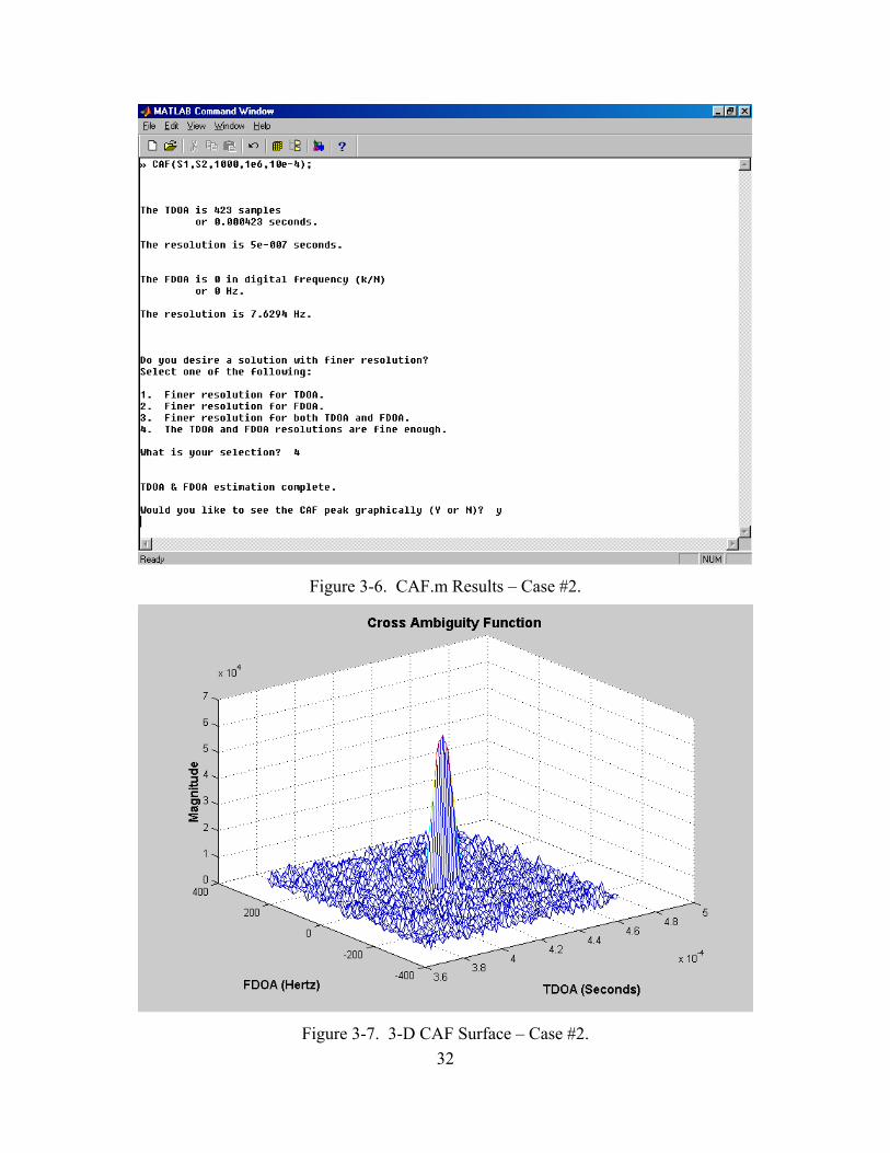
Figure 3-6. CAF.m Results – Case #2.

Figure 3-7. 3-D CAF Surface – Case #2.

32

Figure 3-8. 2-D Cuts Through CAF Surface – Case #2.

TDOA: 423 samples

FDOA: 0 (digital frequency)

Note that there are three main differences between Case #2 and Case #1. First, the

signals have a half-cosine envelope rather than a rectangular one. Second, the signals

have more noise, as seen in their smaller SNRs. Third, the expected TDOA is different:

423 samples or seconds (f44.23 10x −s = 1 MHz). Figures (3-6) through (3-8) show the

results of running this signal set through CAF.m. Again, note that CAF.m computed the

exact solutions since the actual TDOA was an integer number of samples and the FDOA

was zero. Also note the effect of the lower SNRs in this pair of signals. The noise floor

around the CAF peak is significantly higher than in Case #1. Finally, note the shape of

the surface along the TDOA axis. It is more sinusoidal, or perhaps Gaussian, in shape.

This makes sense since the signals’ envelopes were half-cosines. The convolution of two

sinusoidal shapes gives a similar shape. In the next subsection, signal pairs with non-zero

TDOAs and FDOAs will be examined.

33

2. Constant TDOA and Constant FDOA The next two pairs of signals have constant TDOAs and FDOAs embedded within

them. As stated before, constant TDOAs and FDOAs are unrealistic for real-world

geometries. Also, it is impossible to have simultaneously constant TDOAs and FDOAs.

This is because whenever a constant TDOA exists, the FDOA must always be zero!

After all, geometries that produce constant TDOAs are such that the individual Doppler

shifts between each collector and the emitter are identical. The difference between the

Dopplers, the FDOA, is therefore zero! Using signals with constant TDOAs and FDOAs

is, however, quite convenient for testing the operation of the CAF software. For Case #3,

a pair of signals with the following parameters were input into the CAF.m program:

Signal Type: BPSK with rectangular envelope

Carrier Frequency: 0.21 (digital frequency)

Samples Per Bit: 16

Signal-to-Noise Ratio for the two signals: 20 dB & 20 dB

Number of Samples: 65536

TDOA: 358 samples

FDOA: – 0.0005 (digital frequency)

Figures (3-9) through (3-12) show the MATLAB command window results of running

CAF.m on the signals with the above parameters. Again using the assumed value of fs =

1 MHz, the expected TDOA is seconds and the expected TDOA is –500 Hz.

Note that the TDOA was computed exactly after the first iteration. After three more

iterations, the FDOA was also computed exactly. Notice that with each subsequent

iteration, the resolution of the TDOA calculation improves by a factor of two, and the

FDOA resolution improves by a factor of 10, as expected. Figures (3-13) and (3-14)

show the CAF surface in three dimensions and two dimensions, respectively. The plots

are as expected, with the surface’s peak occurring at a TDOA of exactly

seconds, and an FDOA that is within FFT method resolution of –500 Hz.

43.58 10x −

43.58 10x −

34

Figure 3-9. CAF.m Results – Case #3 (1st Iteration).

Figure 3-10. CAF.m Results – Case #3 (2nd Iteration).

35

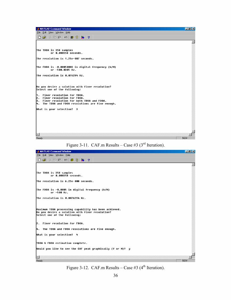
Figure 3-11. CAF.m Results – Case #3 (3rd Iteration).

Figure 3-12. CAF.m Results – Case #3 (4th Iteration).

36

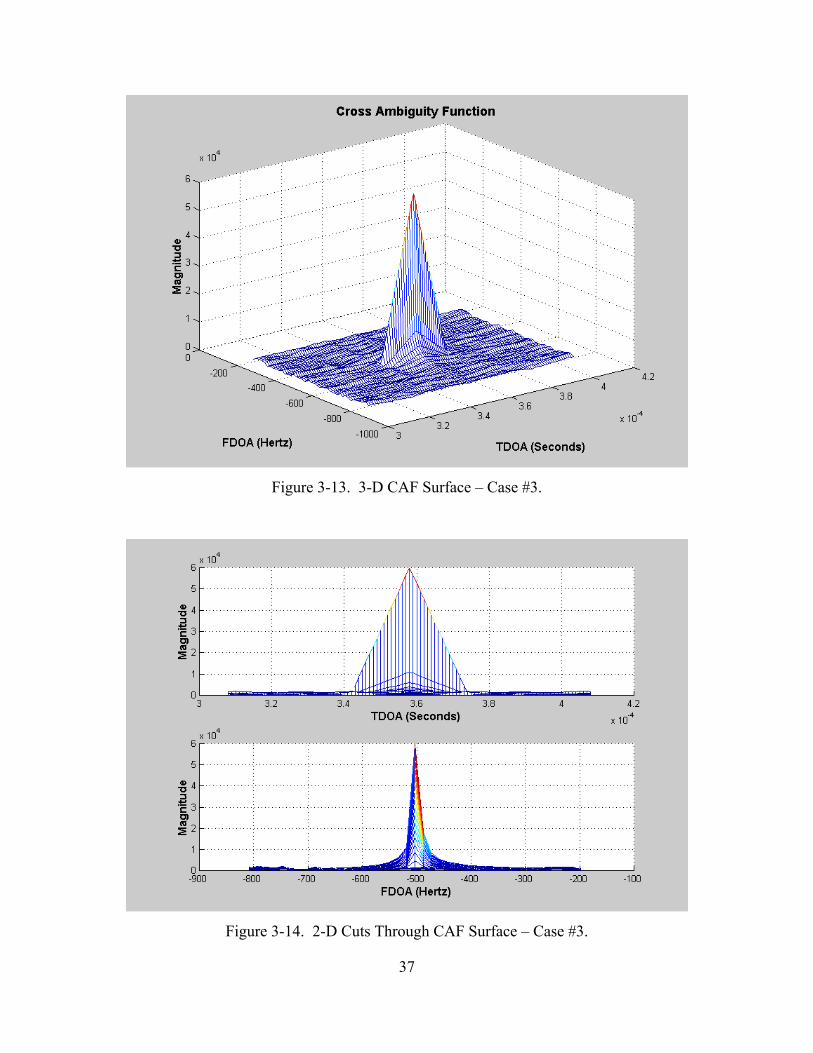
Figure 3-13. 3-D CAF Surface – Case #3.

Figure 3-14. 2-D Cuts Through CAF Surface – Case #3.

37

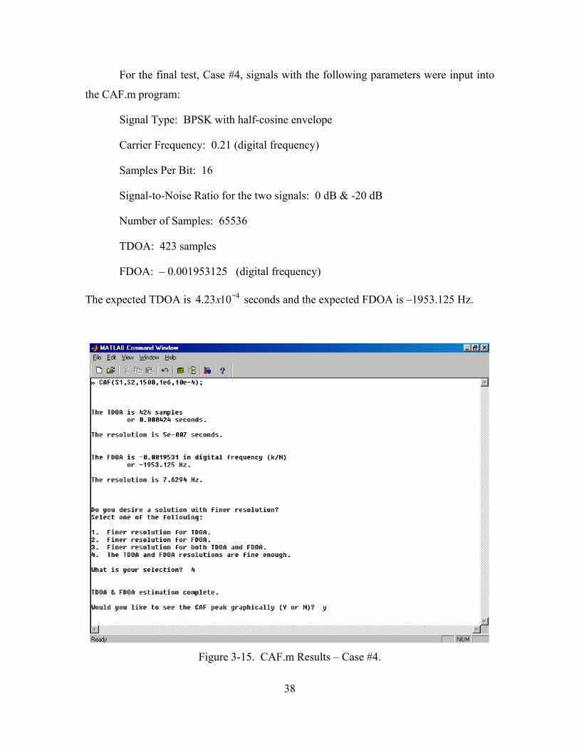
For the final test, Case #4, signals with the following parameters were input into

the CAF.m program:

Signal Type: BPSK with half-cosine envelope

Carrier Frequency: 0.21 (digital frequency)

Samples Per Bit: 16

Signal-to-Noise Ratio for the two signals: 0 dB & -20 dB

Number of Samples: 65536

TDOA: 423 samples

FDOA: – 0.001953125 (digital frequency)

The expected TDOA is seconds and the expected FDOA is –1953.125 Hz. 44.23 10x −

Figure 3-15. CAF.m Results – Case #4.

38

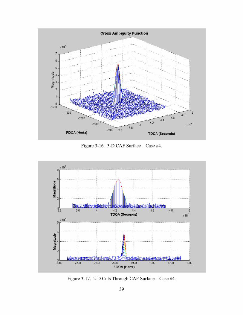
Figure 3-16. 3-D CAF Surface – Case #4.

Figure 3-17. 2-D Cuts Through CAF Surface – Case #4.

39

Figure (3-15) shows the MATLAB command window results after running CAF.m, while

Figures (3-16) and (3-17) show the 3-D and 2-D views of the surface, respectively. Note

that the FDOA was computed exactly after the first iteration. This is because the digital

frequency (–0.001953125) just happens to be associated with an integer frequency bin

number, k. Since digital frequency is defined as kN

x4

, and N = 65536, it follows that k =

128. Note also that the computed TDOA is 4.24 seconds, which is exactly one

sample away from the actual TDOA of seconds. Further iterations of the fine

mode do not yield the exact TDOA. This is likely due to the noise in the signals, which

can introduce errors. This issue will be discussed further in Chapter VI.

410−

10−4.23x

As the four different examples show, the CAF.m and CAF_peak.m programs

function properly to compute accurate TDOAs and FDOAs and display the resulting CAF

surfaces, respectively. As mentioned before, the signal sets used to validate the programs

were not physically realizable due to the artificiality of the constant TDOAs and FDOAs.

Chapter IV provides background information on BPSK signals, and also describes a

Cartesian representation for practical emitter-collector geometries. Chapter V then

describes the approach used in the sig_gen.m program, which generates BPSK signals

based upon user-defined geometries. Several example signal sets are generated and then

input into CAF.m. The results are analyzed and compared with theoretical TDOA and

FDOA calculations.

40

IV. GEOMETRY-SPECIFIC SIGNAL GENERATION Equation Section (Next)

A. BINARY-PHASE-SHIFT-KEYING SIGNALS

The MATLAB code in Appendix B is specifically designed to generate Binary-

Phase-Shift-Keying (BPSK) signals. The BPSK technique is a very common digital

modulation technique, and it is widely used in both military and commercial

communications systems [6].

In BPSK modulation, a sinusoidal carrier wave is modulated by a data signal

consisting of the binary digits “1” and “0.” The data signal shifts the phase of the carrier

waveform to one of two states, either zero or 180° (or π radians). Due to the familiar

trigonometric relationships

sin( ) sin( )cos( ) cos( ),

x xx x

ππ

+ = −+ = −

(4-1)

it is clear that the two possible states in a BPSK system are simply the carrier multiplied

by ±1.

The general analytic expression for a BPSK signal is:

00

( ) cos[2 ( )]1, 2

symi i

t Ts t A f t t

iπ ϕ

≤ ≤= +

= (4-2)

where A is simply the amplitude of the carrier, 0f is the carrier frequency, ( )i tϕ takes on

the values of zero or π, and Tsym is the data symbol period. In binary modulation

techniques, a symbol consists of just one data bit, either 0 or 1. Therefore, in binary

systems such as BPSK, the terms “data symbol” and “symbol period” are synonymous

with “data bit” and “bit period,” respectively. Using Equation (4-2) and bearing

Equations (4-1) in mind, the two possible waveforms transmitted in a BPSK signal are:

1

2 0

( ) cos(2 )( ) cos(2 )

s t A f ts t A f t

ππ

== −

0 (4-3)

Equations (4-3) represent continuous-time or analog signals. In the discrete-time or

sampled case, the following representations are used:

41

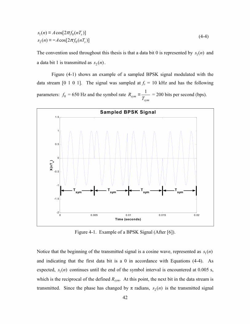
1 0

2 0

( ) cos[2 ( )]( ) cos[2 ( )]

s

s

s n A f nTs n A f nT

ππ

== −

(4-4)

The convention used throughout this thesis is that a data bit 0 is represented by and

a data bit 1 is transmitted as .

1( )s n

2 ( )s n

Figure (4-1) shows an example of a sampled BPSK signal modulated with the

data stream [0 1 0 1]. The signal was sampled at fs = 10 kHz and has the following

parameters: 0f = 650 Hz and the symbol rate 1sym

symR

T= = 200 bits per second (bps).

0 0.005 0.01 0.015 0.02-2

-1.5

-1

-0.5

0

0.5

1

1.5Sampled BPSK Signal

Time (seconds)

X(n

T s)

Tsym Tsym Tsym Tsym

Figure 4-1. Example of a BPSK Signal (After [6]).

Notice that the beginning of the transmitted signal is a cosine wave, represented as

and indicating that the first data bit is a 0 in accordance with Equations (4-4). As

expected, continues until the end of the symbol interval is encountered at 0.005 s,

which is the reciprocal of the defined R

1( )s n

1( )s n

sym. At this point, the next bit in the data stream is

transmitted. Since the phase has changed by π radians, is the transmitted signal 2 ( )s n

42

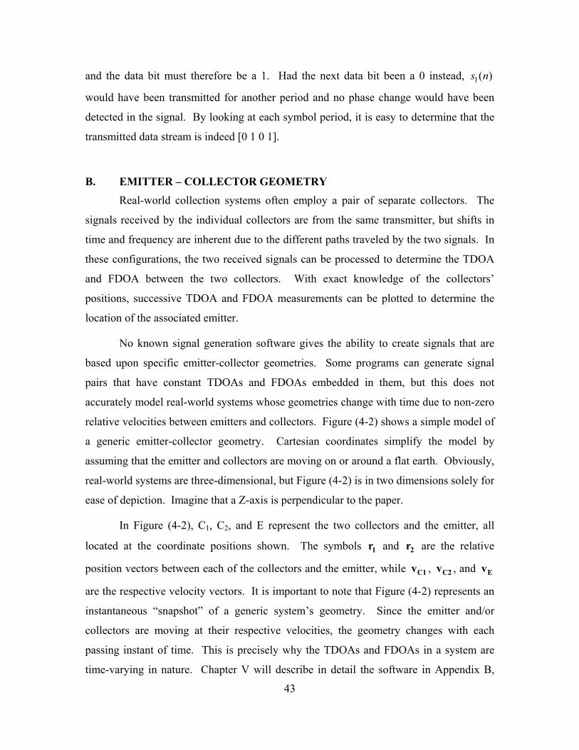
and the data bit must therefore be a 1. Had the next data bit been a 0 instead,

would have been transmitted for another period and no phase change would have been

detected in the signal. By looking at each symbol period, it is easy to determine that the

transmitted data stream is indeed [0 1 0 1].

1( )s n

Ev

B. EMITTER – COLLECTOR GEOMETRY Real-world collection systems often employ a pair of separate collectors. The

signals received by the individual collectors are from the same transmitter, but shifts in

time and frequency are inherent due to the different paths traveled by the two signals. In

these configurations, the two received signals can be processed to determine the TDOA

and FDOA between the two collectors. With exact knowledge of the collectors’

positions, successive TDOA and FDOA measurements can be plotted to determine the

location of the associated emitter.

No known signal generation software gives the ability to create signals that are

based upon specific emitter-collector geometries. Some programs can generate signal

pairs that have constant TDOAs and FDOAs embedded in them, but this does not

accurately model real-world systems whose geometries change with time due to non-zero

relative velocities between emitters and collectors. Figure (4-2) shows a simple model of

a generic emitter-collector geometry. Cartesian coordinates simplify the model by

assuming that the emitter and collectors are moving on or around a flat earth. Obviously,

real-world systems are three-dimensional, but Figure (4-2) is in two dimensions solely for

ease of depiction. Imagine that a Z-axis is perpendicular to the paper.

In Figure (4-2), C1, C2, and E represent the two collectors and the emitter, all

located at the coordinate positions shown. The symbols r and r are the relative

position vectors between each of the collectors and the emitter, while , , and

are the respective velocity vectors. It is important to note that Figure (4-2) represents an

instantaneous “snapshot” of a generic system’s geometry. Since the emitter and/or

collectors are moving at their respective velocities, the geometry changes with each

passing instant of time. This is precisely why the TDOAs and FDOAs in a system are

time-varying in nature. Chapter V will describe in detail the software in Appendix B,

1 2

vC1 C2v

43

which creates geometry-specific signals that capture the time-varying quality of the

TDOA and FDOA. Chapter V will also show that the software in Appendix B works

properly by showing the results of inputting generated signals into the CAF software in

Appendix A.

Figure 4-2. 2-D Emitter-Collector Geometry (After [7]).

C. CALCULATING THEORETICAL TDOA(S) AND FDOA(S) The TDOA between two signals is simply the difference in time that it takes two

signals to travel down their respective paths from the emitter to the associated receivers.

For the geometry shown in Figure (4-2), the TDOA between C1 and C2 is therefore [7]:

,TDOAc−

= 2 1r r (4-5)

44

where −2r r1

is the difference in length between the two paths and c is the speed of

light, at which the signals travel. The vectors r and r are determined simply by

calculating the difference between their x and y coordinates and those of the emitter, so

that

2 1

1

1

2

2

E C

E C

E C

E C

x xy y

x xy y

− = −

− = −

1

2

r

r (4-6)

Now, using the Pythagorean Theorem to define the magnitudes of the path vectors r and

, Equation (4-5) becomes

1

2r

( ) ( ) ( ) ( )2 2 22 2 1

1E C E C E C E CTDOA x x y y x x y y

c = − + − − − + −

21 (4-7)

Of course, Equation (4-7) is strictly for a two-dimensional geometry, but it can easily be

expanded for the 3-D case as well:

( ) ( ) ( )

( ) ( ) ( )

2 22 2

2 21 1

1E C E C E C

E C E C E C

TDOA x x y y z zc

x x y y z z

= − + − + −− − + − + −

22

21

(4-8)

Equation (4-8) is used to calculate the theoretical TDOAs for generated signal pairs. In

Chapter V, theoretical values are compared to the results produced by the CAF software.

The FDOA between two signals is simply the difference between their two

Doppler shifts. From Figure (4-2), the Doppler shift between one of the collectors and

the emitter can be defined as

0 ,ff vc

δ = (4-9)

45

where f0 is the signal’s constant carrier frequency, c is the speed of light, and v is the

(scalar) velocity of closure between the collector and emitter. The velocity of closure is

simply defined as the component of the relative velocity that is along the path of

propagation. Since the collector and emitter velocities and the associated propagation

path are vector quantities, the velocity of closure (v in Equation (4-9)) must be calculated

with the vector dot product as follows [8]:

,v ⋅= v rr

(4-10)

where r represents the path vector and v is the relative velocity between the collector and

emitter, as follows:

Ex Cx

Ey Cy

v vv v

− = −

v (4-11)

In Equation (4-11), v and represent the velocities of the emitter and collector in the

x-direction, while v and v are the y components of the velocities. Now, substituting

Equation (4-10) into Equation (4-9), the Doppler shift for a collector and emitter pair is:

Ex

Ey

Cxv

Cy

0 ,ffc

δ ⋅=

v rr (4-12)

Substituting Equations (4-11) and (4-6) into Equation (4-12) and simplifying produces

the form of the Doppler shift in two dimensions:

( )( ) ( )( )( ) ( )

02 2

Ex Cx E C Ey Cy E C

E C E C

v v x x v v y yffc x x y y

δ − − + − − = − + −

(4-13)

Now, since the FDOA is defined as the difference between the two Doppler shifts

associated with each of the collectors and the emitter, FDOA can be expressed as:

( )( ) ( )( )( ) ( )

( )( ) ( )( )( ) ( )

2 1

2 2 202 2

2 2

1 1 1

2 21 1

Ex C x E C Ey C y E C

E C E C

Ex C x E C Ey C y E C

E C E C

FDOA f f

v v x x v v y yfc x x y y

v v x x v v y y

x x y y

δ δ= −

− − + − −= − + −

− − + − − −− + −

2

1

(4-14)

46

Equation (4-14) is the FDOA for a two dimensional geometry such as that found in

Figure (4-2). It is a straightforward process to extend Equation (4-14) to a three

dimensional geometry:

( )( ) ( )( ) ( )(( ) ( ) ( )

)

( )( ) ( )( ) ( )(( ) ( ) ( )

)

2 2 2 2 202 2 2

2 2 2

1 1 1 1 1

2 2 21 1 1

Ex C x E C Ey C y E C Ez C z E C

E C E C E C

Ex C x E C Ey C y E C Ez C z E C

E C E C E C

FDOA

v v x x v v y y v v z zfc x x y y z z

v v x x v v y y v v z z

x x y y z z

=

− − + − − + − − − + − + −

− − + − − + − − −− + − + −

2

1

(4-15)

Equation (4-15) is used to calculate the theoretical FDOAs for generated signal pairs. In

Chapter V, theoretical values are compared to the results produced by the CAF software.

47

THIS PAGE INTENTIONALLY LEFT BLANK

48

V. IMPLEMENTING THE SIGNAL GENERATOR Equation Section (Next)

A. ANALYSIS OF THE SIGNAL GENERATION SOFTWARE

1. The “Sig_gen.m” Program The program sig_gen.m, listed in Appendix B, is a MATLAB function that

generates pairs of BPSK signals according to user-defined signal parameters and

collector-emitter geometries (of the form described in section IV.B). The function is

invoked in the MATLAB command window with a line of the form:

[Sa1, Sa2, S1, S2] = sig_gen;

There are no input arguments to the function, since the user is queried for all required

parameters. The four output arguments are returned as signal vectors. Sa1 and Sa2 are

the two generated signals in analytic signal format, which is required for subsequent CAF

computations. S1 and S2 are the real-valued, time domain representations of the same

two signals. The real signals are made available in case the user desires to plot the

signals in the time domain, or to look at the periodogram of the real data, etc.

The first section of the function queries the user for all information required to

generate the signals. The user is first asked to input the position and velocity vectors of

the two collectors and the emitter at “time 0.” All position and velocity vectors are

entered in the form “[X Y Z],” where X, Y, and Z denote the components of position and

velocity in each of the 3-D Cartesian directions. Position elements are expressed in

meters and velocity elements are expressed in meters per second. All velocities are

assumed to be constant during the period of collection. Note that “time 0” represents the

beginning of the collection period onboard the collectors. This is an important point that

will be discussed later in this section. The two collectors are assumed to have exactly

synchronized time clocks. With the geometry inputs completed, the user is asked to

define the following signal parameters: carrier frequency (f0) in Hz, sampling frequency

(fs) in Hz, the total number of samples to generate (N), the ratio of symbol energy to

noise power spectral density at each collector (Es_No1 and Es_No2) in dB, and the

symbol rate (Rsym) in symbols per second. The function calculates the sample period

49

directly from the sampling frequency as 1Tsfs

= . Likewise, the symbol period is

calculated as 1TsymRsym

= . Finally, Es_No1 and Es_No2 are converted from dB to ratio

values for future computations. The relationship used is:

100 0

( ) 10logs sE EdBN N

= and 1 ( )

10 0

010

Es dBNsE

N= (5-1)

Next, the speed of light constant (c) is defined as . The

amplitude (A) for the signals is defined to be equal to one. The choice of this value is

simply for convenience; any value could be used here. The average signal power (Ps) is

then calculated, since it will be needed to compute the noise power necessary to achieve

the user’s desired

82.997925x10 /m s

0

sEN

. The definition of a periodic signal’s average power is [6]:

200

0

1 ( )TsP s

T= ∫ t dt (5-2)

Using either or from Equations (4-3) and substituting into Equation (5-2), 1( )s t 2 ( )s t

2 2000

0

1 cos (2 )TsP A f

Tπ= ∫ t dt (5-3)

Simplifying Equation (5-3) leads to the result:

2

2sAP = (5-4)

Sig_gen.m uses Equation (5-4) to calculate the constant Ps directly.

Next, the program creates the noise components of the two signals, according to

the 0

sEN

defined by the user. The noise modeled by the program is Additive White

Gaussian Noise (AWGN), which has a mean of zero and a variance that can be

determined as follows. From [6], Es represents the amount of energy in one symbol, and

can be described as the average signal power times the symbol period:

50

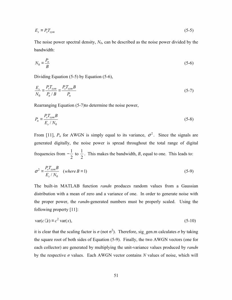
s s symE PT= (5-5)

The noise power spectral density, N0, can be described as the noise power divided by the

bandwidth:

0nPN

B= (5-6)

Dividing Equation (5-5) by Equation (5-6),

0 /s sym s syms

n n

PT PT BEN P B P

= = (5-7)

Rearranging Equation (5-7)to determine the noise power,

0/s sym

ns

PT BP

E N= (5-8)

From [11], Pn for AWGN is simply equal to its variance, . Since the signals are

generated digitally, the noise power is spread throughout the total range of digital

frequencies from

2σ

12

− to 12

. This makes the bandwidth, B, equal to one. This leads to:

2

0(

/s sym

s

PT Bwhere B

E Nσ = 1)= (5-9)

The built-in MATLAB function randn produces random values from a Gaussian

distribution with a mean of zero and a variance of one. In order to generate noise with

the proper power, the randn-generated numbers must be properly scaled. Using the

following property [11]:

2var( ) var( ),c x c x⋅ = (5-10)

it is clear that the scaling factor is σ (not σ2). Therefore, sig_gen.m calculates σ by taking

the square root of both sides of Equation (5-9). Finally, the two AWGN vectors (one for

each collector) are generated by multiplying the unit-variance values produced by randn

by the respective σ values. Each AWGN vector contains N values of noise, which will

51

eventually be added, element-by-element, to the N computed values of the repective

signals. The noise vectors are called Noise1 and Noise2.

Next, the program computes a position matrix for each of the two collectors. This

is a straightforward process since the user provides the starting position and the velocity

for the collectors. The position of a collector at each sample period is simply equal to its

position at the last sample plus a distance equal to the velocity times the sample period.

Using two for loops, sig_gen.m calculates the position of each collector at each sample

time, from 1 to N. The resulting position matrices are N x 3, since a 1 x 3 vector (of the

form [X Y Z]) defines a collector’s position at each of the N sample times.

The next major portion of sig_gen.m computes the position matrix and time

vectors for the emitter. Again, note that time 0 refers to the time onboard the collectors

when the signal collection begins (i.e., nTs, where n = 0). Successive times onboard the

collectors are simply multiples of the sampling period. Since the signal must travel from

the emitter along two separate, non-zero paths to the collectors, it takes different amounts

of time for the signal to travel to the two receivers. Therefore, for samples taken at the

receivers at time nTs, the emitter will have transmitted those portions of the signal at two

different times that are less than nTs by amounts equal to the time it takes the signals to

travel down the respective paths. For example, assume that two collectors are positioned

such that one is 1000 km from the emitter, and the other is 1100 km from the emitter.

The sample taken at the first collector at time 0 will represent the portion of the signal

transmitted at time (0 – 6

81 10

2.997925 10 /x m

x m s), or –0.003336 seconds. On the other hand,

the sample taken at the second collector at time 0 will have been transmitted at time (0 – 6

81.1 10

2.997925 10 /x m

x m s), or –0.003669 seconds. In order to capture this timing arrangement,

the transmit times corresponding to each sample must be tracked for each collector.

Since the emitter may be moving, its position must also be tracked. In order to compute

its position, the transmit times for each sample must be used along with the user-defined

velocity and starting position. Since the position of the emitter is needed to figure out the

distance of the path between it and the collectors, it is clear that the time and position of

52

the emitter are interdependent. They must therefore be determined in an iterative fashion

as described in the next paragraph.

A while loop is used to determine the time and position of the emitter for the first

sample (i.e., the one that arrives at the collector at time 0) at collector number one. The

initial estimates are that the transmit time is 0 and the position is the one entered by the

user. Within the loop, the time is “updated” to be zero minus the path distance divided

by the speed of light. The path distance is that between the collector’s position and the

current estimate of the emitter’s position. The position of the emitter is then computed as

the initial position plus the revised time multiplied by the emitter’s velocity. Note that

the time here is negative, so that the emitter is successively being “walked back” to where

it was when it emitted the first sample. This iterative process continues in the while loop

until two successive estimations of the time differ by less than one period of the carrier

(i.e., 0

1f

). When the loop ends, the computed time and position of the emitter are stored

in a time vector (t1) and position matrix (Pe1), respectively. The process just described

is then repeated in order to determine the time and position of the emitter corresponding

to the first sample at the second collector. The emitter’s time vector and position matrix

associated with collector two are t2 and Pe2, respectively.

53

Next, the “beginning” of the collected signal’s data stream must be determined.

The program compares the emitter times corresponding to the first sample taken at the

two collectors. The earlier of the two times defines the starting point (called StartPoint in

the code) of the data stream. The data symbols are stored as a vector (P) of zeros and

ones, and the correct index into that vector must be computed for each of the two

collectors in order to ensure that bit changes occur at the right times. In the program, the

two indexes are called SymbolIndex1 and SymbolIndex2. Since the earliest transmit time

at the emitter is defined to be the starting point of the data stream, the index into the data

vector is equal to one for the associated collector. The other collector, then, will have an

index into the data vector that is equal to one plus the difference between the two transmit

times divided by the symbol period. For example, assume that transmit times are –1

second for collector number one and –3 seconds for collector number two, and that the

symbol period is one second. Collector two has the earlier transmit time, and therefore

SymbolIndex2 is equal to one. The transmit time for collector one is two seconds later,

which corresponds to two symbol periods. SymbolIndex1 must therefore be equal to

three, or two greater than collector two’s index.

Now that the emitter’s position and transmit time for each collector’s first sample

have been computed, they must be determined for the remaining samples (i.e, numbers 2

through N). This is accomplished with a for loop running from 2 to N. Nested inside is a

while loop very similar to the ones used to compute the transmit times and positions for

the first sample (described above). The main difference is that for each sample, the initial

estimate of the emitter’s position is equal to the position for the previous sample plus the

sample period times the emitter’s velocity. Then, inside the while loop, the transmit time

is computed as the sample time (nTs) minus the path distance divided by the speed of

light. The path distance here is that between the collector’s position at time nTs and the

current estimate of the emitter’s position. The position of the emitter is then computed as

the initial position plus the elapsed time (i.e., the difference between the transmit time for

the first sample and the estimate of the current sample’s transmit time) multiplied by the

emitter’s velocity. The while loop ends when the difference between two successive time

estimates is less than one period of the carrier. When the overall for loop is done, the t1

vector contains N elements, each of which represents the time at which the associated

sample was actually transmitted by the emitter. Likewise, the Pe1 matrix contains N (1 x

3) vectors, each representing the emitter’s position at the corresponding transmit times in

t1. The process just described is then repeated for collector two, so that all the values for

the t2 vector and Pe2 matrix are calculated.

54

Next, the data sequence is randomly generated and stored in the vector P. The

possible values are 0 and 1, and they are assumed to be equally likely to occur.

Therefore, MATLAB’s rand function is used to create a vector of random numbers

between 0 and 1. All numbers that are less than 0.5 are called 1s, and all numbers greater

than 0.5 are called 0s. Note that prior to creating the random data bits, the program

initializes the rand function to a specific seed. This is useful for testing purposes because

it ensures that the same random data stream is generated every time the program is run.

The line “rand('seed',5);” can simply be removed if a different random data stream is

desired each time. Or, greater control could be given to the user by making the seed

number an input to the program. Alternatively, if a user desired to have a specific data

stream, the entire vector P could be made an input argument.

Finally, the actual transmitted signals are generated, sample-by-sample. Equation

(4-2) is computed directly for each collector’s signal, with t equal to the transmit times

computed and stored in the vectors t1 and t2. The phase component, ( )i tϕ , is equal to the

associated data bit stored in P (indexed by SymbolIndex1 and SymbolIndex2) multiplied

by п (and hence giving values equal to either 0 or п, as required). The noise elements

from Noise1 and Noise2 are also added to their respective signal components. For each

of the two signals, a for loop is used to compute all N samples. For each sample’s

computation, a test is made to determine if the total elapsed time has crossed into the next

symbol period. If so, the appropriate index is incremented by one, so that the next data

bit is obtained from P. If the next symbol period has not yet been reached, then the

current data bit remains in effect. At the end of the two for loops, the vectors S1 and S2

contain the real-valued sampled signals that are received by collectors one and two,

respectively. Using MATLAB’s hilbert function, Sa1 and Sa2 are computed. They

represent the complex-valued analytic signal representations of S1 and S2, respectively.

Note that although the Hilbert Transform is defined as in Equation (2-4), the hilbert

function in MATLAB computes the analytic signal, Equation (2-3), directly. The four

resulting signal vectors are returned to the user as output arguments.

After the signals have been created, sig_gen.m calls the tdoa_fdoa.m function,

which computes and displays the theoretical values of the TDOA and FDOA at the

beginning and end of the collection period. The toda_fdoa.m program is briefly

described in the next section.

2. The “Tdoa_fdoa.m” Program The tdoa_fdoa.m program takes a number of input arguments and computes the

expected TDOA and FDOA at both the beginning and end of a signal collection. Again,

real-world geometries produce time-varying TDOAs and FDOAs, so it is convenient to

know what the expected range of values for each will be. The function’s input arguments

are: the carrier frequency (f0), the emitter’s beginning and ending position vectors

55

relative to each signal (Pe1_b, Pe1_e, Pe2_b, and Pe2_e), the beginning and ending

position vectors for the two collectors (Pc1_b, Pc1_e, Pc2_b, and Pc2_e), and the

velocity vectors for the emitter (Ve) and collectors (Vc1 and Vc2). The function then

computes the beginning and ending TDOAs and FDOAs by implementing Equations

(4-8) and (4-15), respectively. The results are then displayed in the MATLAB command

window.

B. EXAMPLE GEOMETRIES AND SIGNAL SETS In order to test the sig_gen.m function and ensure that it operates correctly,

several different signal sets were generated with the software, and then input into CAF.m

to compare actual TDOA and FDOA measurements with the theoretical values calculated

by tdoa_fdoa.m. The following subsections document the results of five different pairs of

signals. The first three show the results of simple geometries that produce different

combinations of constant and time-varying TDOAs and FDOAs. The last two

subsections show the results of simulating real-world geometries with spaceborne and

airborne collectors.

1. Constant TDOA and Zero FDOA As pointed out in section III.C.2, it is impossible for an emitter-collector

geometry to produce simultaneously constant, non-zero TDOAs and FDOAs, because a

constant TDOA causes the associated FDOA to be zero. To illustrate this point, a pair of

signals was generated with the parameters and geometry inputs listed in Figure (5-1),

which is the MATLAB command window after running the sig_gen.m function. The

geometry is such that the emitter and both colletors are on a line in the x-direction. Both

collectors are to the right of, and moving away from, the emitter. Note that in MATLAB,

“1e5” is mathematically equivalent to 1 1 50x . Also note that the defined geometry and

velocities for this example are not necessarily realistic. They just represent a simple case

showing that a constant TDOA leads to an FDOA of zero. Finally, notice that the

sampling frequency is less than the carrier frequency. This does not adversely impact the

CAF computations since the goal is to find the TDOA and FDOA, not to preserve the

56

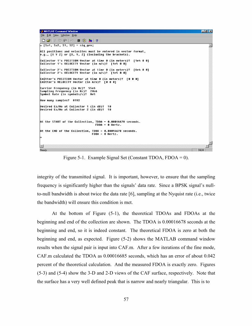
Figure 5-1. Example Signal Set (Constant TDOA, FDOA = 0).

integrity of the transmitted signal. It is important, however, to ensure that the sampling

frequency is significantly higher than the signals’ data rate. Since a BPSK signal’s null-

to-null bandwidth is about twice the data rate [6], sampling at the Nyquist rate (i.e., twice

the bandwidth) will ensure this condition is met.

At the bottom of Figure (5-1), the theoretical TDOAs and FDOAs at the

beginning and end of the collection are shown. The TDOA is 0.00016678 seconds at the

beginning and end, so it is indeed constant. The theoretical FDOA is zero at both the

beginning and end, as expected. Figure (5-2) shows the MATLAB command window

results when the signal pair is input into CAF.m. After a few iterations of the fine mode,

CAF.m calculated the TDOA as 0.00016685 seconds, which has an error of about 0.042

percent of the theoretical calculation. And the measured FDOA is exactly zero. Figures

(5-3) and (5-4) show the 3-D and 2-D views of the CAF surface, respectively. Note that

the surface has a very well defined peak that is narrow and nearly triangular. This is to

57

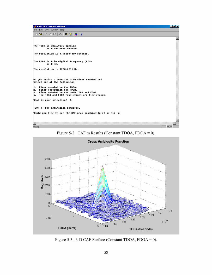
Figure 5-2. CAF.m Results (Constant TDOA, FDOA = 0).

Figure 5-3. 3-D CAF Surface (Constant TDOA, FDOA = 0).

58

Figure 5-4. 2-D Cuts Through CAF Surface (Constant TDOA, FDOA = 0).

be expected for signals with rectangular envelopes, and for situations where the TDOA is

constant. The next section will show how a time-varying TDOA affects the resulting

CAF surface.

2. Time-Varying TDOA and Constant FDOA Figure (5-5) shows the geometry and parameters used to generate a pair of signals

that has a time-varying TDOA and a constant FDOA. Again, the geometry and signal

parameters are not at all realistic, but the values were chosen in order to exaggerate the

effect that a time-varying TDOA has on the CAF surface. For comparison purposes, the

values were also chosen so that the ending TDOA would be somewhat close to the

constant TDOA of the previous section. As Figure (5-5) shows, the TDOA is clearly

time-varying, since it is 0.00010007 seconds at the beginning of the collection and

0.00016642 seconds at the end. The FDOA is a constant value equal to –21831.767 Hz.

59

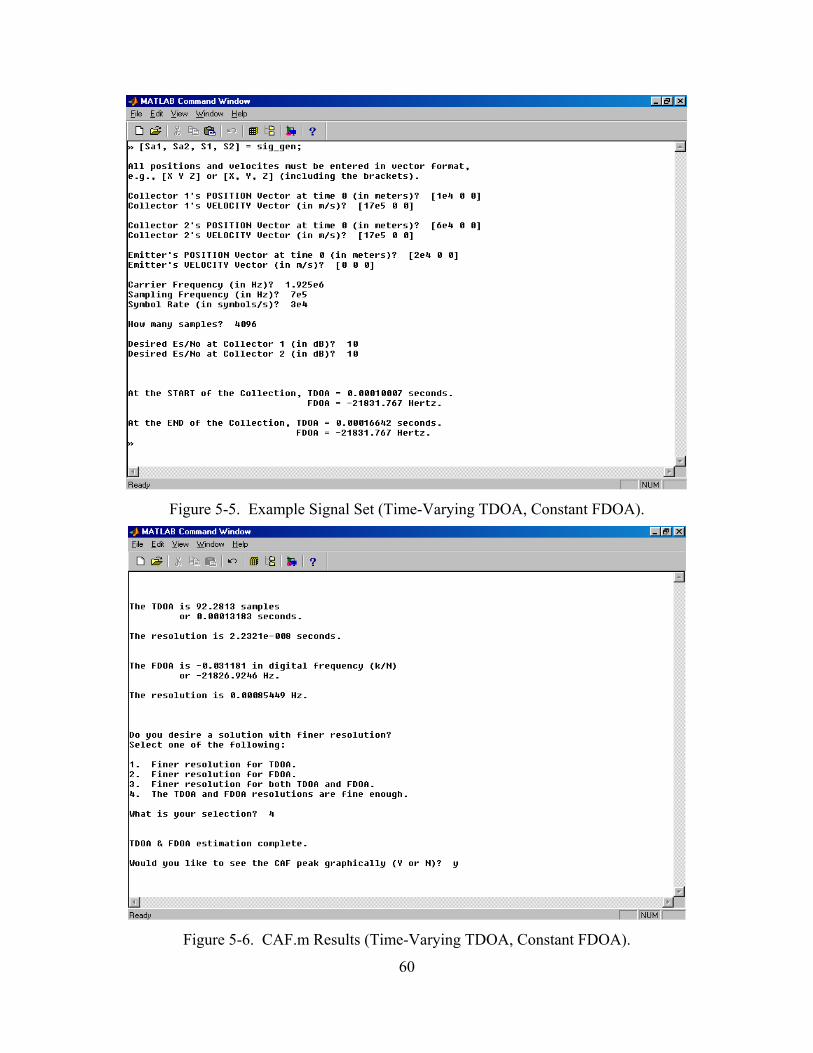
Figure 5-5. Example Signal Set (Time-Varying TDOA, Constant FDOA).

Figure 5-6. CAF.m Results (Time-Varying TDOA, Constant FDOA).

60

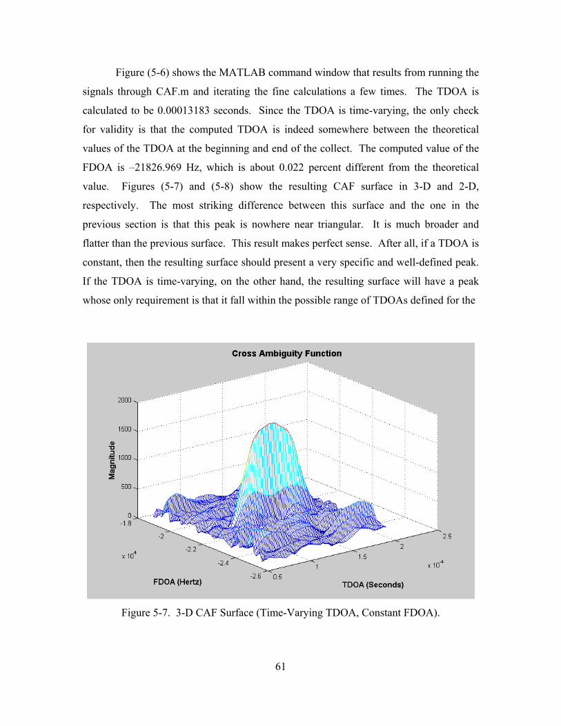
Figure (5-6) shows the MATLAB command window that results from running the

signals through CAF.m and iterating the fine calculations a few times. The TDOA is

calculated to be 0.00013183 seconds. Since the TDOA is time-varying, the only check

for validity is that the computed TDOA is indeed somewhere between the theoretical

values of the TDOA at the beginning and end of the collect. The computed value of the

FDOA is –21826.969 Hz, which is about 0.022 percent different from the theoretical

value. Figures (5-7) and (5-8) show the resulting CAF surface in 3-D and 2-D,

respectively. The most striking difference between this surface and the one in the

previous section is that this peak is nowhere near triangular. It is much broader and

flatter than the previous surface. This result makes perfect sense. After all, if a TDOA is

constant, then the resulting surface should present a very specific and well-defined peak.

If the TDOA is time-varying, on the other hand, the resulting surface will have a peak

whose only requirement is that it fall within the possible range of TDOAs defined for the

Figure 5-7. 3-D CAF Surface (Time-Varying TDOA, Constant FDOA).

61

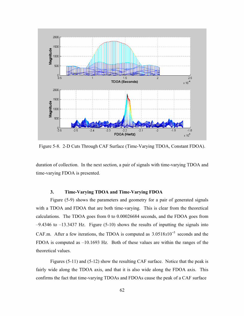
Figure 5-8. 2-D Cuts Through CAF Surface (Time-Varying TDOA, Constant FDOA).

duration of collection. In the next section, a pair of signals with time-varying TDOA and

time-varying FDOA is presented.

3. Time-Varying TDOA and Time-Varying FDOA Figure (5-9) shows the parameters and geometry for a pair of generated signals

with a TDOA and FDOA that are both time-varying. This is clear from the theoretical

calculations. The TDOA goes from 0 to 0.00026684 seconds, and the FDOA goes from

–9.4346 to –13.3437 Hz. Figure (5-10) shows the results of inputting the signals into

CAF.m. After a few iterations, the TDOA is computed as seconds and the

FDOA is computed as –10.1693 Hz. Both of these values are within the ranges of the

theoretical values.

53.0518 10x −

Figures (5-11) and (5-12) show the resulting CAF surface. Notice that the peak is

fairly wide along the TDOA axis, and that it is also wide along the FDOA axis. This

confirms the fact that time-varying TDOAs and FDOAs cause the peak of a CAF surface

62

Figure 5-9. Example Signal Set (Time-Varying TDOA and FDOA).

Figure 5-10. CAF.m Results (Time-Varying TDOA and FDOA).

63

Figure 5-11. 3-D CAF Surface (Time-Varying TDOA and FDOA).

Figure 5-12. 2-D Cuts Through CAF Surface (Time-Varying TDOA and FDOA).

64

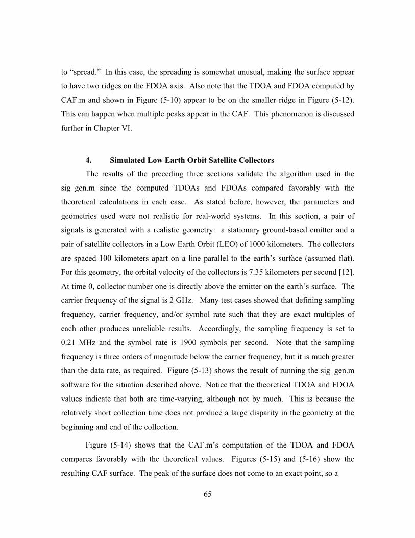
to “spread.” In this case, the spreading is somewhat unusual, making the surface appear

to have two ridges on the FDOA axis. Also note that the TDOA and FDOA computed by

CAF.m and shown in Figure (5-10) appear to be on the smaller ridge in Figure (5-12).

This can happen when multiple peaks appear in the CAF. This phenomenon is discussed

further in Chapter VI.

4. Simulated Low Earth Orbit Satellite Collectors The results of the preceding three sections validate the algorithm used in the

sig_gen.m since the computed TDOAs and FDOAs compared favorably with the

theoretical calculations in each case. As stated before, however, the parameters and

geometries used were not realistic for real-world systems. In this section, a pair of

signals is generated with a realistic geometry: a stationary ground-based emitter and a

pair of satellite collectors in a Low Earth Orbit (LEO) of 1000 kilometers. The collectors

are spaced 100 kilometers apart on a line parallel to the earth’s surface (assumed flat).

For this geometry, the orbital velocity of the collectors is 7.35 kilometers per second [12].

At time 0, collector number one is directly above the emitter on the earth’s surface. The

carrier frequency of the signal is 2 GHz. Many test cases showed that defining sampling

frequency, carrier frequency, and/or symbol rate such that they are exact multiples of

each other produces unreliable results. Accordingly, the sampling frequency is set to

0.21 MHz and the symbol rate is 1900 symbols per second. Note that the sampling

frequency is three orders of magnitude below the carrier frequency, but it is much greater

than the data rate, as required. Figure (5-13) shows the result of running the sig_gen.m

software for the situation described above. Notice that the theoretical TDOA and FDOA

values indicate that both are time-varying, although not by much. This is because the

relatively short collection time does not produce a large disparity in the geometry at the

beginning and end of the collection.

Figure (5-14) shows that the CAF.m’s computation of the TDOA and FDOA

compares favorably with the theoretical values. Figures (5-15) and (5-16) show the

resulting CAF surface. The peak of the surface does not come to an exact point, so a

65

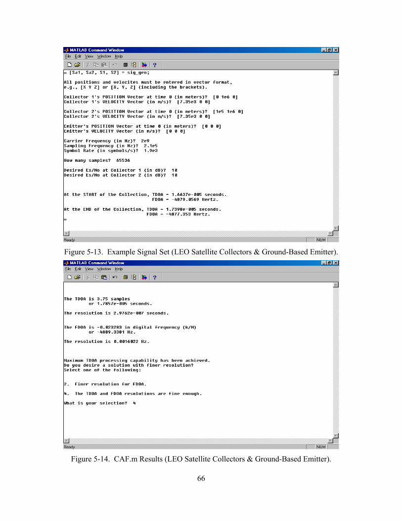
Figure 5-13. Example Signal Set (LEO Satellite Collectors & Ground-Based Emitter).

Figure 5-14. CAF.m Results (LEO Satellite Collectors & Ground-Based Emitter).

66

Figure 5-15. 3-D CAF Surface (LEO Satellite Collectors & Ground-Based Emitter).

Figure 5-16. 2-D Cuts Through CAF Surface (LEO Collectors & Ground Emitter).

67

small amount of smearing is evident. On the FDOA axis in Figure (5-16), the slope of

the surface on the left hand side is not quite as steep as the slope on the right hand side.

This indicates a slight smearing to the left, which makes sense given the range of FDOAs

predicted in Figure (5-14).

5. Simulated Airborne Collectors In this section, another real-world system is simulated: a pair of airborne

collectors and a ground-based emitter. The collectors are assumed to be mounted on an

aircraft with the same dimensions and characteristics of an EP-3 Aries. One collector is

assumed to be mounted in the nose of the aircraft, and the other collector in the tail. This

provides for maximum separation of the collectors onboard the aircraft. From [13], the

length of an EP-3 is 105 feet, 11 inches; its maximum speed is 473 knots; and its

maximum altitude is 28,000 feet. For purposes of collection, the assumed speed is 300

knots, and the assumed altitude is 25,000 feet. The airplane is assumed to be flying

parallel to a coastline at a distance of 100 nautical miles from the coast.

Figure (5-17) shows the results of running sig_gen.m for the situation described

above. Note that all geometric inputs have been converted to meters and meters per

second, as appropriate. For the Cartesian coordinate system in this case, the x-direction

is parallel to the coastline, the y-direction is altitude, and the z-direction is perpendicular

to the coastline in the plane of the earth’s surface (i.e., it measures lateral distance from

the coastline). The signal has a carrier frequency of 4 GHz and a symbol rate of 1.2

megabits per second, and it is sampled at 1.1 GHz. Notice that the resulting theoretical

values of TDOA and FDOA are constant. This is only because the geometry does not

change much during such a small collection time. If a much larger number of samples

were taken, the TDOA and FDOA would show more change. Also notice that the

FDOA, at –0.35708 Hz is a miniscule fraction of the sampling frequency!

Figure (5-18) shows the results obtained by running CAF.m. The computed

TDOA and FDOA compare reasonably well with the theoretical values. The computed

FDOA differs from its theoretical value by a minus sign, or about 0.7 Hz total. Although

this is a large error percentage-wise, it is reasonable when considering that the FDOA

68

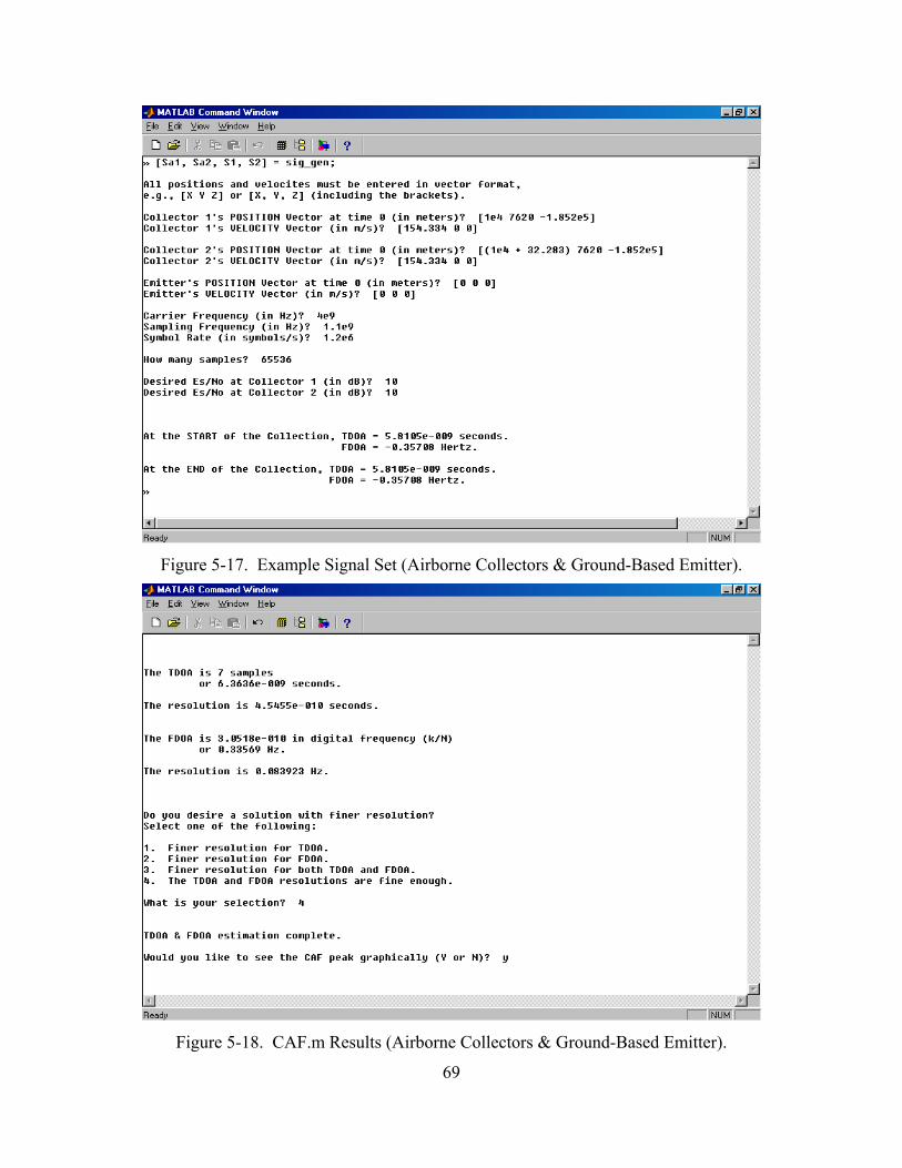
Figure 5-17. Example Signal Set (Airborne Collectors & Ground-Based Emitter).

Figure 5-18. CAF.m Results (Airborne Collectors & Ground-Based Emitter).

69

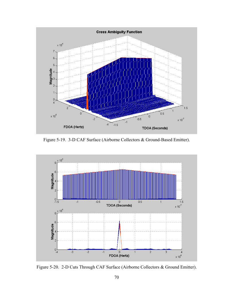
Figure 5-19. 3-D CAF Surface (Airborne Collectors & Ground-Based Emitter).

Figure 5-20. 2-D Cuts Through CAF Surface (Airborne Collectors & Ground Emitter).

70

resolution for N = 65536 is 91.1 10

65536x Hz

samples = 16,784.7 Hz per sample! In this context,

CAF.m did a reasonable job of picking out a tiny FDOA.

Figures (5-19) and (5-20) show the resulting CAF surface. The peak occurs at the

expected TDOA of roughly 6 nanoseconds, but the FDOA at the peak is 0 Hz. This

makes sense considering the discussion in the previous paragraph. For this situation, the

FDOA is such a small fraction of the sampling frequency that the resolution achieved

with N = 65536 is not sufficient to show the correct FDOA graphically. Recall that

CAF_peak.m uses the FFT method to generate the CAF values and plot the surface. This

is why CAF.m is able to determine the FDOA, while the resulting plot is unable to show

it. This section, along with the previous one, has shown that the programs created for this

thesis are indeed able to model signals with realistic parameters and emitter-collector

geometries, as well as compute the embedded TDOA and FDOA with a good degree of

accuracy. Section V.C below will demonstrate the CAF’s ability to detect signals.

C. USING THE CAF FOR SIGNAL DETECTION

71

As shown throughout this thesis, the CAF is able to compute the TDOA and

FDOA between two receivers collecting signals from the same emitter. The TDOA and

FDOA information can then be used to locate the emitter. In many cases, the presence of

the signal(s) may be known prior to collection. The CAF itself, however, can also be

used to detect the presence of a signal by processing a pair of collections and looking for

peaks above the noise floor. This can be useful for Low Probability of Detection (LPD)

signals, which may be transmitted at very low 0

sEN

levels. As an example, consider the

LEO collector system modeled in section V.B.4 above. Using all of the parameters in

Figure (5-13), the 0

sEN

was successively reduced to show the effects on CAF

computations and the CAF surface. Figures (5-21) through (5-25) show the 2-D cuts

through the CAF surface for 0

sEN

levels of –20 dB, –40 dB, –45 dB, –50 dB, and –55 dB,

respectively. The –20 dB level does not appear to have affected the CAF surface much at

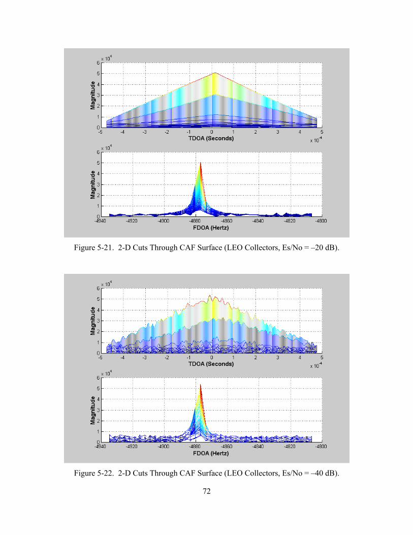
Figure 5-21. 2-D Cuts Through CAF Surface (LEO Collectors, Es/No = –20 dB).

Figure 5-22. 2-D Cuts Through CAF Surface (LEO Collectors, Es/No = –40 dB).

72

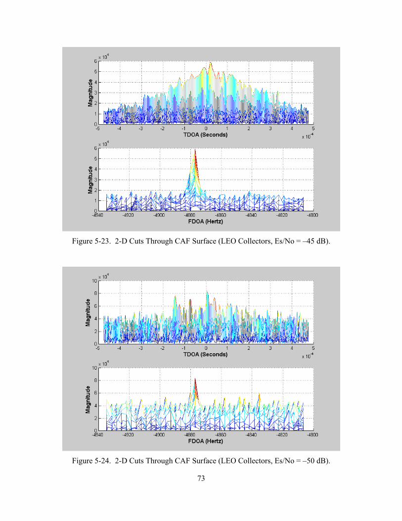
Figure 5-23. 2-D Cuts Through CAF Surface (LEO Collectors, Es/No = –45 dB).

Figure 5-24. 2-D Cuts Through CAF Surface (LEO Collectors, Es/No = –50 dB).

73

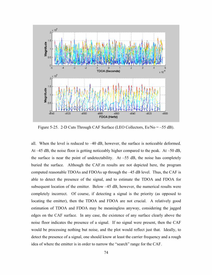
Figure 5-25. 2-D Cuts Through CAF Surface (LEO Collectors, Es/No = –55 dB).

all. When the level is reduced to –40 dB, however, the surface is noticeable deformed.

At –45 dB, the noise floor is getting noticeably higher compared to the peak. At –50 dB,

the surface is near the point of undetectability. At –55 dB, the noise has completely

buried the surface. Although the CAF.m results are not depicted here, the program

computed reasonable TDOAs and FDOAs up through the –45 dB level. Thus, the CAF is

able to detect the presence of the signal, and to estimate the TDOA and FDOA for

subsequent location of the emitter. Below –45 dB, however, the numerical results were

completely incorrect. Of course, if detecting a signal is the priority (as opposed to

locating the emitter), then the TDOA and FDOA are not crucial. A relatively good

estimation of TDOA and FDOA may be meaningless anyway, considering the jagged

edges on the CAF surface. In any case, the existence of any surface clearly above the

noise floor indicates the presence of a signal. If no signal were present, then the CAF

would be processing nothing but noise, and the plot would reflect just that. Ideally, to

detect the presence of a signal, one should know at least the carrier frequency and a rough

idea of where the emitter is in order to narrow the “search” range for the CAF.

74

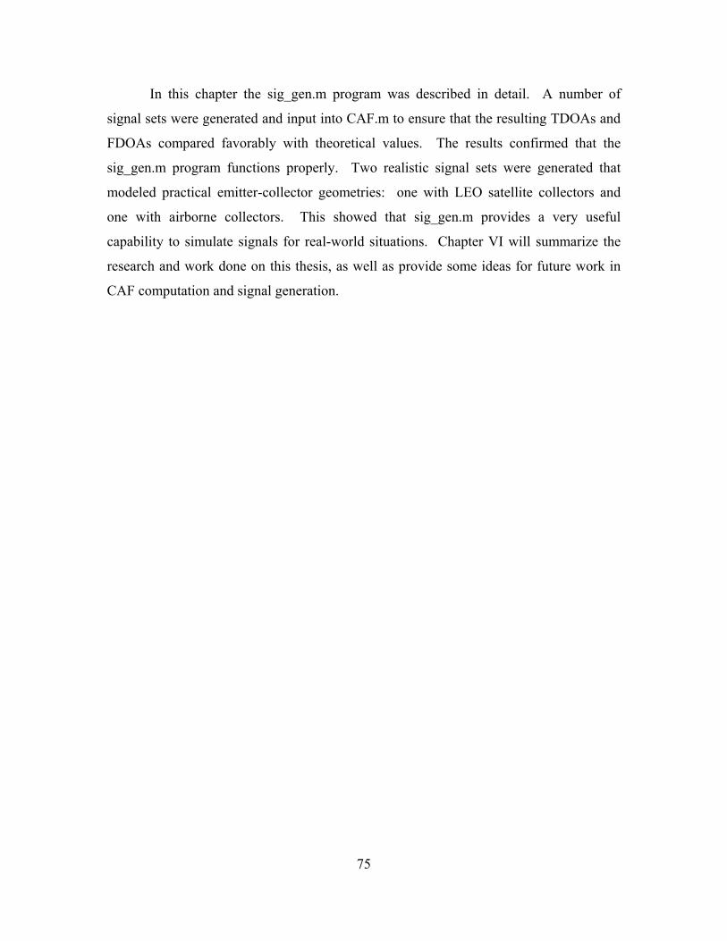
In this chapter the sig_gen.m program was described in detail. A number of

signal sets were generated and input into CAF.m to ensure that the resulting TDOAs and

FDOAs compared favorably with theoretical values. The results confirmed that the

sig_gen.m program functions properly. Two realistic signal sets were generated that

modeled practical emitter-collector geometries: one with LEO satellite collectors and

one with airborne collectors. This showed that sig_gen.m provides a very useful

capability to simulate signals for real-world situations. Chapter VI will summarize the

research and work done on this thesis, as well as provide some ideas for future work in

CAF computation and signal generation.

75

THIS PAGE INTENTIONALLY LEFT BLANK

76

VI. CONCLUSIONS Equation Section (Next)

A. SUMMARY OF FINDINGS

There were two goals for this thesis. One was to develop MATLAB software that

implements CAF techniques to efficiently compute the TDOA and FDOA between two

sampled signals. The second goal was to develop software capable of generating pairs of

signals that are based upon user-defined parameters and emitter-collector geometries.

The resulting programs, listed in Appendices A and B, achieved these two goals.

Many real-world collection systems utilize CAF techniques to locate radio

frequency transmitters. These systems enjoy the benefit of enormous computing

resources (e.g., supercomputers) with which to accomplish the CAF processing. The

software developed for this thesis (Appendix A), however, provides a new capability for

users to conduct CAF computations with the much more limited processing power of a

desktop PC. In order to minimize processing burden, the CAF software splits the

computations into coarse and fine modes. The coarse mode implements the algorithm

described in [1]. An analysis of the computational complexities of three direct CAF

calculation methods showed that utilizing an explicit summation is the most efficient

method for the fine mode. Limitations of a desktop PC may restrict the size of the

sampled signals that can be processed, but realistic simulations are definitely possible.

The software in Appendix B provides a new capability for users to produce

realistic BPSK signal sets that might be transmitted and collected by real-world systems.

This capability, combined with the CAF software, allows a user to model practical

systems to determine whether or not particular signals could be detected and/or their

emitters located. For example, a proposed LPD emitter could be simulated to analyze its

effectiveness against CAF processing. These programs could be useful in many other

applications as well.

B. FUTURE WORK There are a number of ways that future research could build upon the work

described in this thesis. One could analyze the theoretical processing gain provided by

77

the CAF, and compare it to the results of actual test cases. For the CAF software, the

coarse mode described in section III.B.1 only works for positive TDOAs. The coarse

algorithm could be reviewed and possibly modified to handle negative TDOAs. During

coarse mode processing in CAF.m, the estimations of TDOA and FDOA are associated

with the single largest magnitude computed. In reality, coarse mode processing can

produce multiple peaks and the correct TDOA and FDOA could be associated with any

of them. The coarse algorithm in CAF.m could be modified so that it processes more

than just the largest peak. This would require determining a threshold (based upon noise

and other factors), above which a peak would be considered a candidate.

The fine mode in CAF.m could be automated so that the program itself would

decide to what degree of resolution the TDOA and FDOA should be computed, rather

than have the user decide how many times to run the fine mode. Reference [1] describes

how the standard deviation of the CAF surface in the TDOA and FDOA directions can be

used to determine the maximum degree of accuracy that can be expected. The standard

deviations are dependent upon bandwidths, total collection time, and signal-to-noise

ratios. Defining the maximum accuracy then sets the maximum resolution required for

computations.

There are a couple of ways that the signal generation software could be enhanced.

For example, it could be expanded to be able to generate other kinds of signals.

Sig_gen.m is written so that it would be straightforward to add the ability to generate

higher-order PSK signals (4-PSK, etc.). Other signal types might be added as well

(Amplitude-Shift-Keying, etc.). Also, while the 3-D Cartesian coordinate system used in

sig_gen.m provides a fairly realistic model, especially for short collect times, the program

could be modified to use earth-centered coordinates instead. This would be complicated,

but would clearly make simulations even more realistic.

78

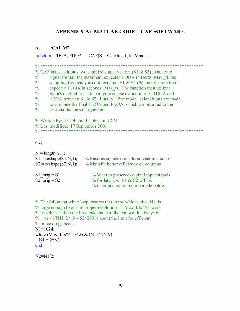
APPENDIX A: MATLAB CODE – CAF SOFTWARE

A. “CAF.M” function [TDOA, FDOA] = CAF(S1, S2, Max_f, fs, Max_t); % ********************************************************************* % CAF takes as inputs two sampled signal vectors (S1 & S2) in analytic % signal format, the maximum expected FDOA in Hertz (Max_f), the % sampling frequency used to generate S1 & S2 (fs), and the maximum % expected TDOA in seconds (Max_t). The function then utilizes % Stein's method in [1] to compute coarse estimations of TDOA and % FDOA between S1 & S2. Finally, "fine mode" calcualtions are made % to compute the final TDOA and FDOA, which are returned to the % user via the output arguments. % Written by: LCDR Joe J. Johnson, USN % Last modified: 17 September 2001 % ********************************************************************* clc; N = length(S1); S1 = reshape(S1,N,1); % Ensures signals are column vectors due to S2 = reshape(S2,N,1); % Matlab's better efficiency on columns S1_orig = S1; % Want to preserve original input signals S2_orig = S2; % for later use; S1 & S2 will be % manipulated in the fine mode below. % The following while loop ensures that the sub-block size, N1, is % large enough to ensure proper resolution. If Max_f/fs*N1 were % less than 1, then the Freq calculated at the end would always be % + or - 1/N1! 2^19 = 524288 is about the limit for efficient % processing speed. N1=1024; while (Max_f/fs*N1 < 2) & (N1 < 2^19) N1 = 2*N1; end N2=N1/2;

79

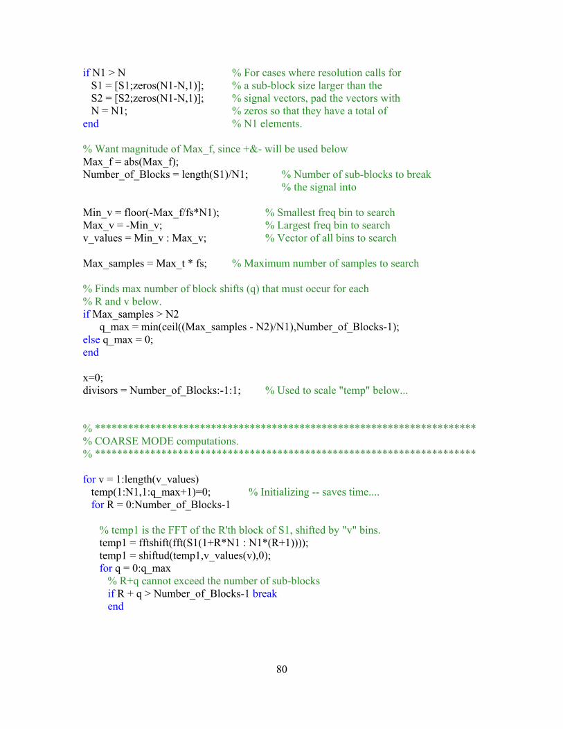
if N1 > N % For cases where resolution calls for S1 = [S1;zeros(N1-N,1)]; % a sub-block size larger than the S2 = [S2;zeros(N1-N,1)]; % signal vectors, pad the vectors with N = N1; % zeros so that they have a total of end % N1 elements. % Want magnitude of Max_f, since +&- will be used below Max_f = abs(Max_f); Number_of_Blocks = length(S1)/N1; % Number of sub-blocks to break % the signal into Min_v = floor(-Max_f/fs*N1); % Smallest freq bin to search Max_v = -Min_v; % Largest freq bin to search v_values = Min_v : Max_v; % Vector of all bins to search Max_samples = Max_t * fs; % Maximum number of samples to search % Finds max number of block shifts (q) that must occur for each % R and v below. if Max_samples > N2 q_max = min(ceil((Max_samples - N2)/N1),Number_of_Blocks-1); else q_max = 0; end x=0; divisors = Number_of_Blocks:-1:1; % Used to scale "temp" below... % ********************************************************************* % COARSE MODE computations. % ********************************************************************* for v = 1:length(v_values) temp(1:N1,1:q_max+1)=0; % Initializing -- saves time.... for R = 0:Number_of_Blocks-1 % temp1 is the FFT of the R'th block of S1, shifted by "v" bins. temp1 = fftshift(fft(S1(1+R*N1 : N1*(R+1)))); temp1 = shiftud(temp1,v_values(v),0); for q = 0:q_max % R+q cannot exceed the number of sub-blocks if R + q > Number_of_Blocks-1 break end

80

% FFT of the (R+q)'th block of S2 temp2 = fftshift(fft([S2(1+(R+q)*N1 : N2 + N1*(R+q));... zeros(N2,1)])); % Multiplies temp1 & temp2, FFTs the product, then adds to % previous values for the same value of q (but different R) temp(:,q+1) = temp(:,q+1) + ... abs(fftshift(fft(temp1.*conj(temp2)))); end end % Each value of q was used a different # of times, so they must be % scaled properly. for q_index = 1:q_max+1 temp(:,q_index) = temp(:,q_index) / divisors(q_index); end % If combination of current v and any q provides a greater value % than the previous max, then remember m, Q, & V. if max(max(temp))>x x = max(max(temp)); [m Q] = find(temp == max(max(temp))); % Must do this since q starts at 0, but Matlab doesn't allow for % zero indexing. Q = Q - 1; V = v_values(v); end end % Coarse estimate of TDOA (in # of samples) TDOA_Coarse = Q * N1 + (-N2+1 + m); % Coarse estimate of FDOA (in Freq Bin #) FDOA_Coarse = V/N1*N; % The following 3 lines can be used to display the coarse estimates, % if desired. %disp(['The coarse TDOA estimate is: ', num2str(TDOA_Coarse),... % ' samples.']); %disp(['The coarse FDOA estimate is: ', num2str(FDOA_Coarse/N),... % ' (digital frequency).']);

81

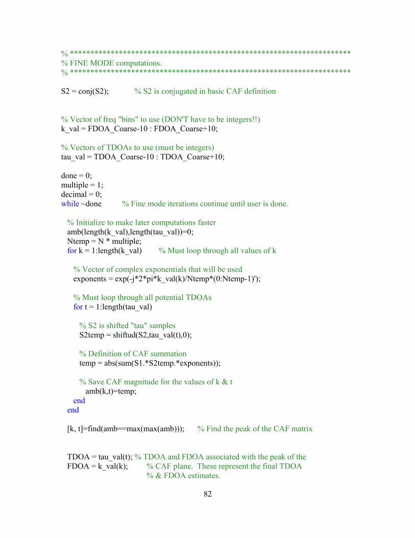
% ********************************************************************* % FINE MODE computations. % ********************************************************************* S2 = conj(S2); % S2 is conjugated in basic CAF definition % Vector of freq "bins" to use (DON'T have to be integers!!) k_val = FDOA_Coarse-10 : FDOA_Coarse+10; % Vectors of TDOAs to use (must be integers) tau_val = TDOA_Coarse-10 : TDOA_Coarse+10; done = 0; multiple = 1; decimal = 0; while ~done % Fine mode iterations continue until user is done. % Initialize to make later computations faster amb(length(k_val),length(tau_val))=0; Ntemp = N * multiple; for k = 1:length(k_val) % Must loop through all values of k % Vector of complex exponentials that will be used exponents = exp(-j*2*pi*k_val(k)/Ntemp*(0:Ntemp-1)'); % Must loop through all potential TDOAs for t = 1:length(tau_val) % S2 is shifted "tau" samples S2temp = shiftud(S2,tau_val(t),0); % Definition of CAF summation temp = abs(sum(S1.*S2temp.*exponents)); % Save CAF magnitude for the values of k & t amb(k,t)=temp; end end [k, t]=find(amb==max(max(amb))); % Find the peak of the CAF matrix TDOA = tau_val(t); % TDOA and FDOA associated with the peak of the FDOA = k_val(k); % CAF plane. These represent the final TDOA % & FDOA estimates.

82

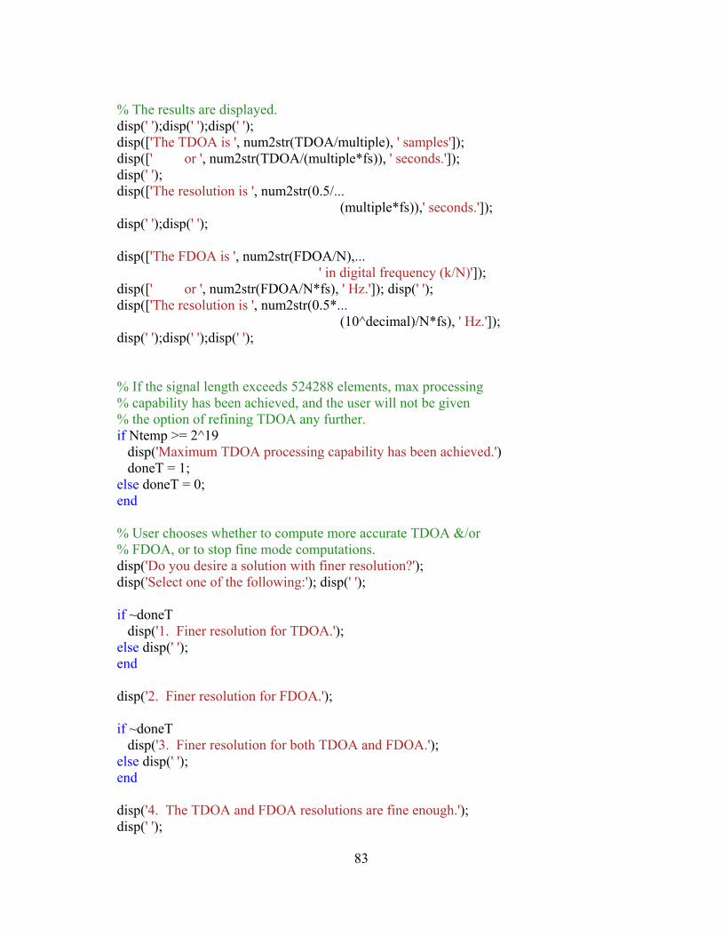
% The results are displayed. disp(' ');disp(' ');disp(' '); disp(['The TDOA is ', num2str(TDOA/multiple), ' samples']); disp([' or ', num2str(TDOA/(multiple*fs)), ' seconds.']); disp(' '); disp(['The resolution is ', num2str(0.5/... (multiple*fs)),' seconds.']); disp(' ');disp(' '); disp(['The FDOA is ', num2str(FDOA/N),... ' in digital frequency (k/N)']); disp([' or ', num2str(FDOA/N*fs), ' Hz.']); disp(' '); disp(['The resolution is ', num2str(0.5*... (10^decimal)/N*fs), ' Hz.']); disp(' ');disp(' ');disp(' '); % If the signal length exceeds 524288 elements, max processing % capability has been achieved, and the user will not be given % the option of refining TDOA any further. if Ntemp >= 2^19 disp('Maximum TDOA processing capability has been achieved.') doneT = 1; else doneT = 0; end % User chooses whether to compute more accurate TDOA &/or % FDOA, or to stop fine mode computations. disp('Do you desire a solution with finer resolution?'); disp('Select one of the following:'); disp(' '); if ~doneT disp('1. Finer resolution for TDOA.'); else disp(' '); end disp('2. Finer resolution for FDOA.'); if ~doneT disp('3. Finer resolution for both TDOA and FDOA.'); else disp(' '); end disp('4. The TDOA and FDOA resolutions are fine enough.'); disp(' ');

83

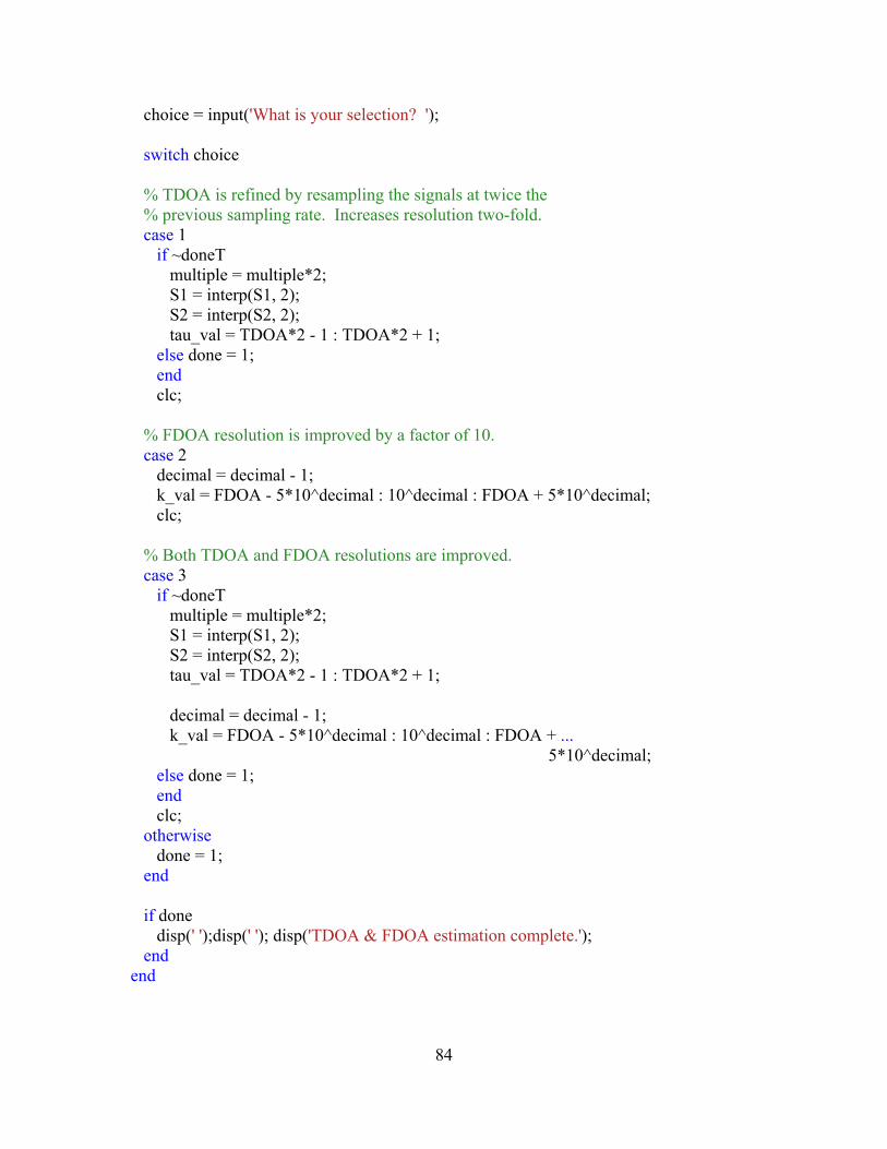
choice = input('What is your selection? '); switch choice % TDOA is refined by resampling the signals at twice the % previous sampling rate. Increases resolution two-fold. case 1 if ~doneT multiple = multiple*2; S1 = interp(S1, 2); S2 = interp(S2, 2); tau_val = TDOA*2 - 1 : TDOA*2 + 1; else done = 1; end clc; % FDOA resolution is improved by a factor of 10. case 2 decimal = decimal - 1; k_val = FDOA - 5*10^decimal : 10^decimal : FDOA + 5*10^decimal; clc; % Both TDOA and FDOA resolutions are improved. case 3 if ~doneT multiple = multiple*2; S1 = interp(S1, 2); S2 = interp(S2, 2); tau_val = TDOA*2 - 1 : TDOA*2 + 1; decimal = decimal - 1; k_val = FDOA - 5*10^decimal : 10^decimal : FDOA + ... 5*10^decimal; else done = 1; end clc; otherwise done = 1; end if done disp(' ');disp(' '); disp('TDOA & FDOA estimation complete.'); end end

84

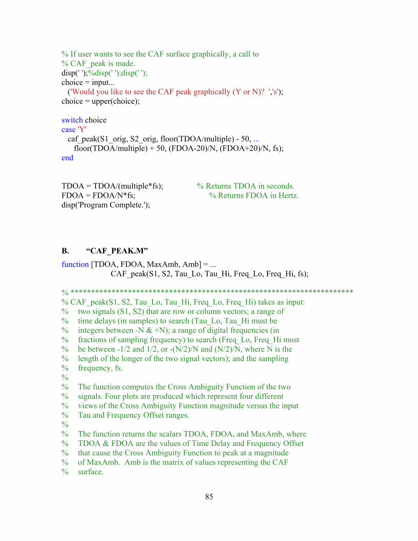
% If user wants to see the CAF surface graphically, a call to % CAF_peak is made. disp(' ');%disp(' ');disp(' '); choice = input... ('Would you like to see the CAF peak graphically (Y or N)? ','s'); choice = upper(choice); switch choice case 'Y' caf_peak(S1_orig, S2_orig, floor(TDOA/multiple) - 50, ... floor(TDOA/multiple) + 50, (FDOA-20)/N, (FDOA+20)/N, fs); end TDOA = TDOA/(multiple*fs); % Returns TDOA in seconds. FDOA = FDOA/N*fs; % Returns FDOA in Hertz. disp('Program Complete.');

B. “CAF_PEAK.M” function [TDOA, FDOA, MaxAmb, Amb] = ... CAF_peak(S1, S2, Tau_Lo, Tau_Hi, Freq_Lo, Freq_Hi, fs); % ********************************************************************* % CAF_peak(S1, S2, Tau_Lo, Tau_Hi, Freq_Lo, Freq_Hi) takes as input: % two signals (S1, S2) that are row or column vectors; a range of % time delays (in samples) to search (Tau_Lo, Tau_Hi must be % integers between -N & +N); a range of digital frequencies (in % fractions of sampling frequency) to search (Freq_Lo, Freq_Hi must % be between -1/2 and 1/2, or -(N/2)/N and (N/2)/N, where N is the % length of the longer of the two signal vectors); and the sampling % frequency, fs. % % The function computes the Cross Ambiguity Function of the two % signals. Four plots are produced which represent four different % views of the Cross Ambiguity Function magnitude versus the input % Tau and Frequency Offset ranges. % % The function returns the scalars TDOA, FDOA, and MaxAmb, where % TDOA & FDOA are the values of Time Delay and Frequency Offset % that cause the Cross Ambiguity Function to peak at a magnitude % of MaxAmb. Amb is the matrix of values representing the CAF % surface.

85

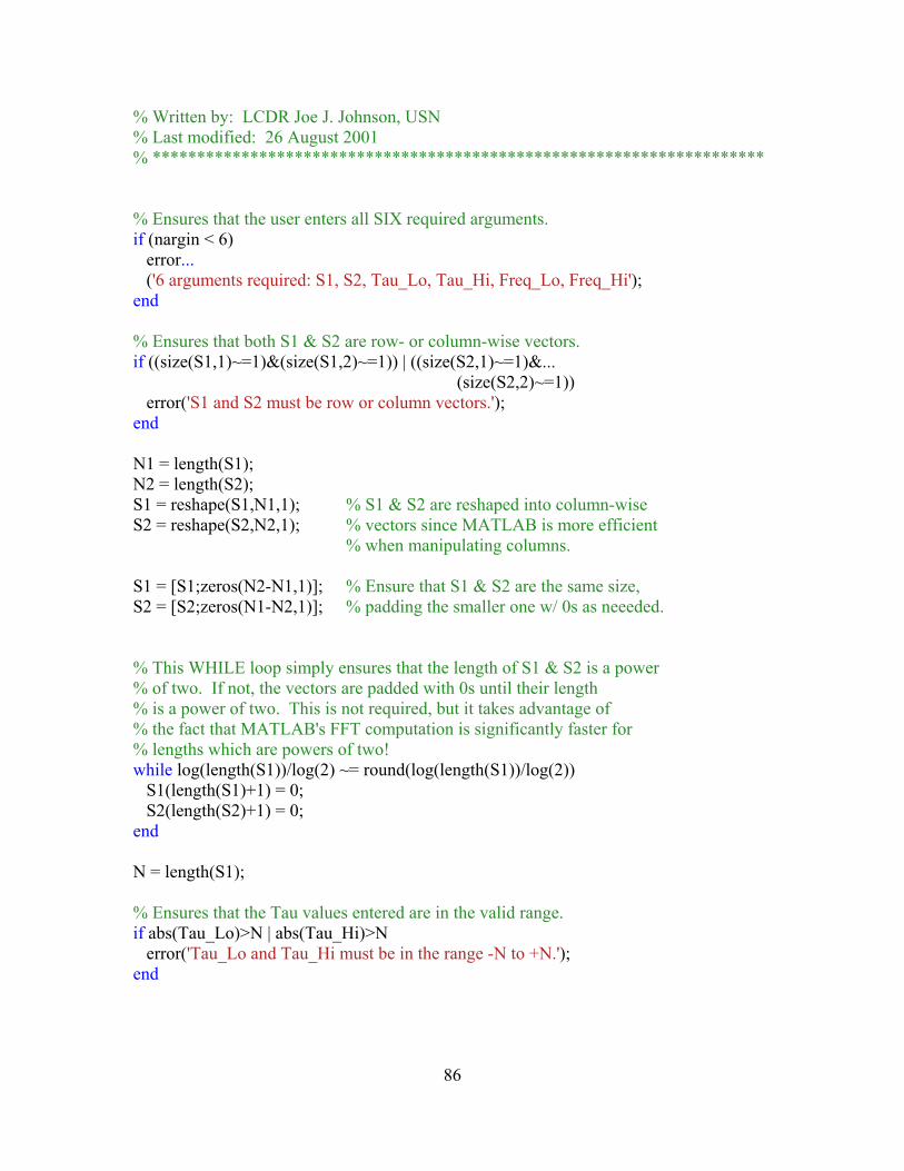
% Written by: LCDR Joe J. Johnson, USN % Last modified: 26 August 2001 % ********************************************************************* % Ensures that the user enters all SIX required arguments. if (nargin < 6) error... ('6 arguments required: S1, S2, Tau_Lo, Tau_Hi, Freq_Lo, Freq_Hi'); end % Ensures that both S1 & S2 are row- or column-wise vectors. if ((size(S1,1)~=1)&(size(S1,2)~=1)) | ((size(S2,1)~=1)&... (size(S2,2)~=1)) error('S1 and S2 must be row or column vectors.'); end N1 = length(S1); N2 = length(S2); S1 = reshape(S1,N1,1); % S1 & S2 are reshaped into column-wise S2 = reshape(S2,N2,1); % vectors since MATLAB is more efficient % when manipulating columns. S1 = [S1;zeros(N2-N1,1)]; % Ensure that S1 & S2 are the same size, S2 = [S2;zeros(N1-N2,1)]; % padding the smaller one w/ 0s as neeeded. % This WHILE loop simply ensures that the length of S1 & S2 is a power % of two. If not, the vectors are padded with 0s until their length % is a power of two. This is not required, but it takes advantage of % the fact that MATLAB's FFT computation is significantly faster for % lengths which are powers of two! while log(length(S1))/log(2) ~= round(log(length(S1))/log(2)) S1(length(S1)+1) = 0; S2(length(S2)+1) = 0; end N = length(S1); % Ensures that the Tau values entered are in the valid range. if abs(Tau_Lo)>N | abs(Tau_Hi)>N error('Tau_Lo and Tau_Hi must be in the range -N to +N.'); end

86

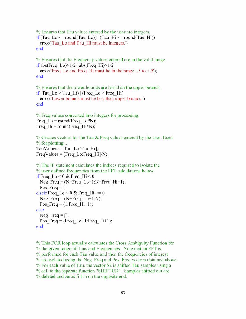
% Ensures that Tau values entered by the user are integers. if (Tau_Lo ~= round(Tau_Lo)) | (Tau_Hi ~= round(Tau_Hi)) error('Tau_Lo and Tau_Hi must be integers.') end % Ensures that the Frequency values entered are in the valid range. if abs(Freq_Lo)>1/2 | abs(Freq_Hi)>1/2 error('Freq_Lo and Freq_Hi must be in the range -.5 to +.5'); end % Ensures that the lower bounds are less than the upper bounds. if (Tau_Lo > Tau_Hi) | (Freq_Lo > Freq_Hi) error('Lower bounds must be less than upper bounds.') end % Freq values converted into integers for processing. Freq_Lo = round(Freq_Lo*N); Freq_Hi = round(Freq_Hi*N); % Creates vectors for the Tau & Freq values entered by the user. Used % for plotting... TauValues = [Tau_Lo:Tau_Hi]; FreqValues = [Freq_Lo:Freq_Hi]/N; % The IF statement calculates the indices required to isolate the % user-defined frequencies from the FFT calculations below. if Freq_Lo < 0 & Freq_Hi < 0 Neg_Freq = (N+Freq_Lo+1:N+Freq_Hi+1); Pos_Freq = []; elseif Freq_Lo < 0 & Freq_Hi >= 0 Neg_Freq = (N+Freq_Lo+1:N); Pos_Freq = (1:Freq_Hi+1); else Neg_Freq = []; Pos_Freq = (Freq_Lo+1:Freq_Hi+1); end % This FOR loop actually calculates the Cross Ambiguity Function for % the given range of Taus and Frequencies. Note that an FFT is % performed for each Tau value and then the frequencies of interest % are isolated using the Neg_Freq and Pos_Freq vectors obtained above. % For each value of Tau, the vector S2 is shifted Tau samples using a % call to the separate function "SHIFTUD". Samples shifted out are % deleted and zeros fill in on the opposite end.

87

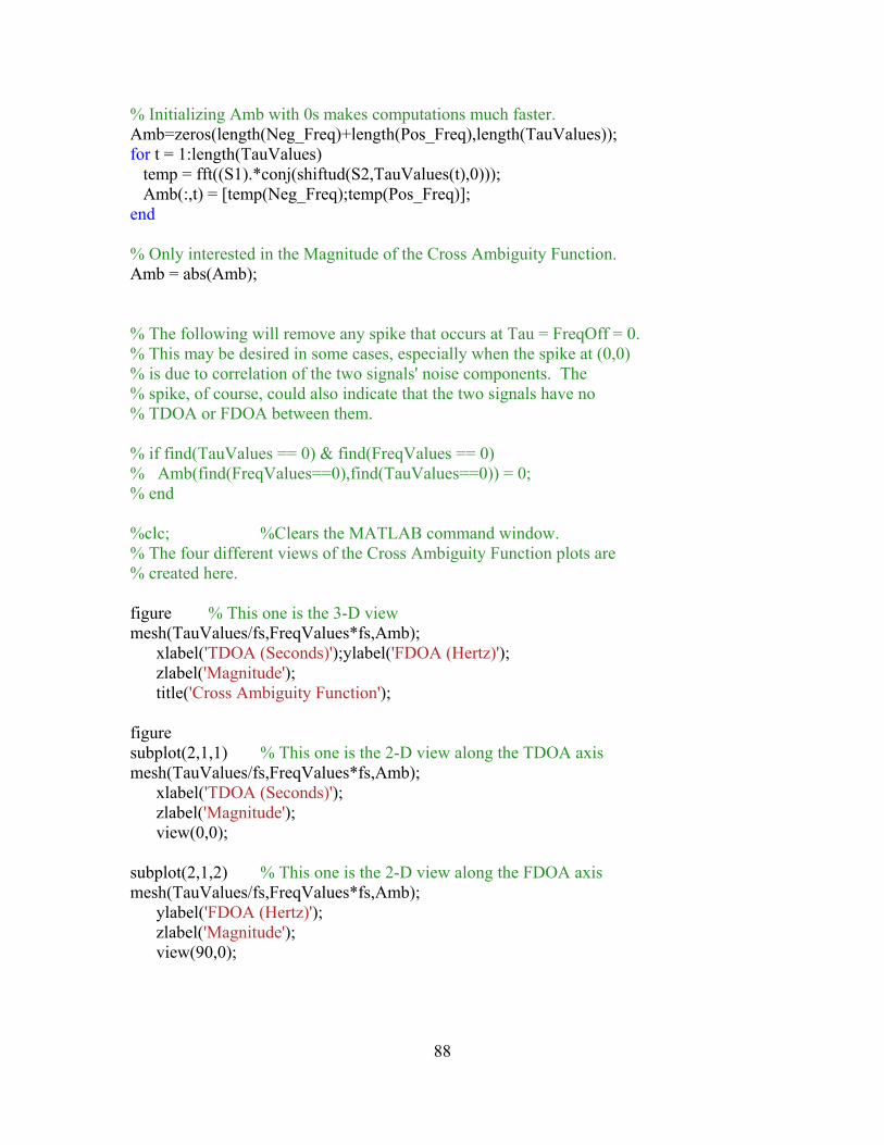
% Initializing Amb with 0s makes computations much faster. Amb=zeros(length(Neg_Freq)+length(Pos_Freq),length(TauValues)); for t = 1:length(TauValues) temp = fft((S1).*conj(shiftud(S2,TauValues(t),0))); Amb(:,t) = [temp(Neg_Freq);temp(Pos_Freq)]; end % Only interested in the Magnitude of the Cross Ambiguity Function. Amb = abs(Amb); % The following will remove any spike that occurs at Tau = FreqOff = 0. % This may be desired in some cases, especially when the spike at (0,0) % is due to correlation of the two signals' noise components. The % spike, of course, could also indicate that the two signals have no % TDOA or FDOA between them. % if find(TauValues == 0) & find(FreqValues == 0) % Amb(find(FreqValues==0),find(TauValues==0)) = 0; % end %clc; %Clears the MATLAB command window. % The four different views of the Cross Ambiguity Function plots are % created here. figure % This one is the 3-D view mesh(TauValues/fs,FreqValues*fs,Amb); xlabel('TDOA (Seconds)');ylabel('FDOA (Hertz)'); zlabel('Magnitude'); title('Cross Ambiguity Function'); figure subplot(2,1,1) % This one is the 2-D view along the TDOA axis mesh(TauValues/fs,FreqValues*fs,Amb); xlabel('TDOA (Seconds)'); zlabel('Magnitude'); view(0,0); subplot(2,1,2) % This one is the 2-D view along the FDOA axis mesh(TauValues/fs,FreqValues*fs,Amb); ylabel('FDOA (Hertz)'); zlabel('Magnitude'); view(90,0);

88

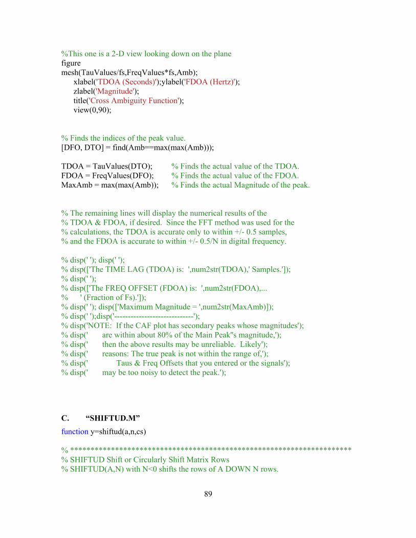
%This one is a 2-D view looking down on the plane figure mesh(TauValues/fs,FreqValues*fs,Amb); xlabel('TDOA (Seconds)');ylabel('FDOA (Hertz)'); zlabel('Magnitude'); title('Cross Ambiguity Function'); view(0,90); % Finds the indices of the peak value. [DFO, DTO] = find(Amb==max(max(Amb))); TDOA = TauValues(DTO); % Finds the actual value of the TDOA. FDOA = FreqValues(DFO); % Finds the actual value of the FDOA. MaxAmb = max(max(Amb)); % Finds the actual Magnitude of the peak. % The remaining lines will display the numerical results of the % TDOA & FDOA, if desired. Since the FFT method was used for the % calculations, the TDOA is accurate only to within +/- 0.5 samples, % and the FDOA is accurate to within +/- 0.5/N in digital frequency. % disp(' '); disp(' '); % disp(['The TIME LAG (TDOA) is: ',num2str(TDOA),' Samples.']); % disp(' '); % disp(['The FREQ OFFSET (FDOA) is: ',num2str(FDOA),... % ' (Fraction of Fs).']); % disp(' '); disp(['Maximum Magnitude = ',num2str(MaxAmb)]); % disp(' ');disp('-----------------------------'); % disp('NOTE: If the CAF plot has secondary peaks whose magnitudes'); % disp(' are within about 80% of the Main Peak''s magnitude,'); % disp(' then the above results may be unreliable. Likely'); % disp(' reasons: The true peak is not within the range of,'); % disp(' Taus & Freq Offsets that you entered or the signals'); % disp(' may be too noisy to detect the peak.');

C. “SHIFTUD.M” function y=shiftud(a,n,cs) % ********************************************************************* % SHIFTUD Shift or Circularly Shift Matrix Rows % SHIFTUD(A,N) with N<0 shifts the rows of A DOWN N rows.

89

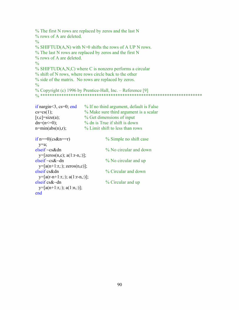
% The first N rows are replaced by zeros and the last N % rows of A are deleted. % % SHIFTUD(A,N) with N>0 shifts the rows of A UP N rows. % The last N rows are replaced by zeros and the first N % rows of A are deleted. % % SHIFTUD(A,N,C) where C is nonzero performs a circular % shift of N rows, where rows circle back to the other % side of the matrix. No rows are replaced by zeros. % % Copyright (c) 1996 by Prentice-Hall, Inc. – Reference [9] % ********************************************************************* if nargin<3, cs=0; end % If no third argument, default is False cs=cs(1); % Make sure third argument is a scalar [r,c]=size(a); % Get dimensions of input dn=(n<=0); % dn is True if shift is down n=min(abs(n),r); % Limit shift to less than rows if n==0|(cs&n==r) % Simple no shift case y=a; elseif ~cs&dn % No circular and down y=[zeros(n,c); a(1:r-n,:)]; elseif ~cs&~dn % No circular and up y=[a(n+1:r,:); zeros(n,c)]; elseif cs&dn % Circular and down y=[a(r-n+1:r,:); a(1:r-n,:)]; elseif cs&~dn % Circular and up y=[a(n+1:r,:); a(1:n,:)]; end

90

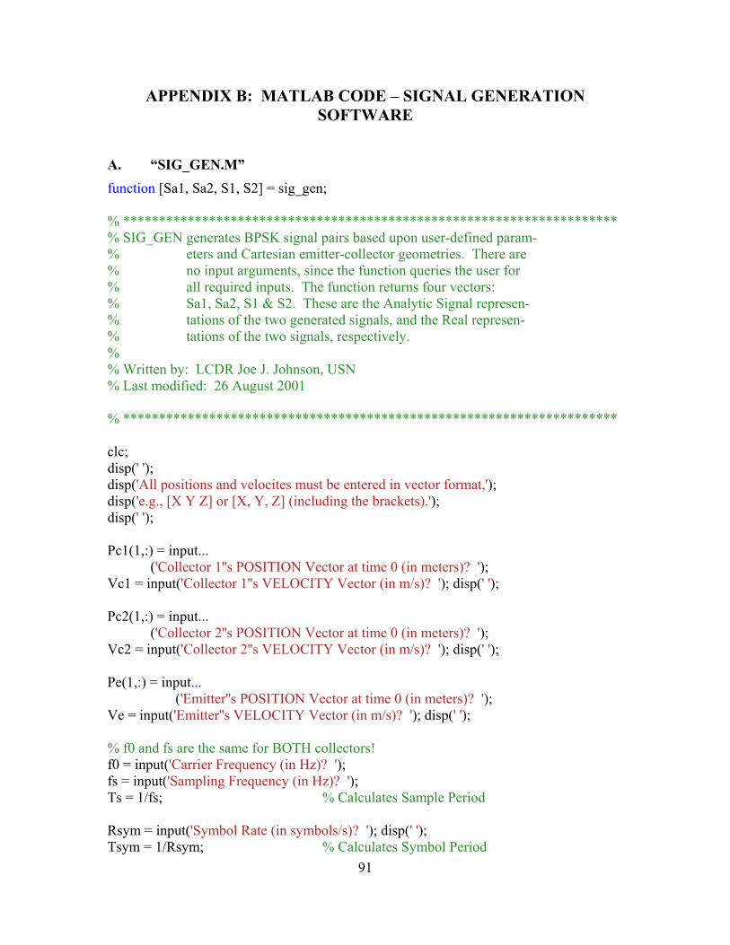
APPENDIX B: MATLAB CODE – SIGNAL GENERATION SOFTWARE

A. “SIG_GEN.M” function [Sa1, Sa2, S1, S2] = sig_gen; % ********************************************************************* % SIG_GEN generates BPSK signal pairs based upon user-defined param- % eters and Cartesian emitter-collector geometries. There are % no input arguments, since the function queries the user for % all required inputs. The function returns four vectors: % Sa1, Sa2, S1 & S2. These are the Analytic Signal represen- % tations of the two generated signals, and the Real represen- % tations of the two signals, respectively. % % Written by: LCDR Joe J. Johnson, USN % Last modified: 26 August 2001 % ********************************************************************* clc; disp(' '); disp('All positions and velocites must be entered in vector format,'); disp('e.g., [X Y Z] or [X, Y, Z] (including the brackets).'); disp(' '); Pc1(1,:) = input... ('Collector 1''s POSITION Vector at time 0 (in meters)? '); Vc1 = input('Collector 1''s VELOCITY Vector (in m/s)? '); disp(' '); Pc2(1,:) = input... ('Collector 2''s POSITION Vector at time 0 (in meters)? '); Vc2 = input('Collector 2''s VELOCITY Vector (in m/s)? '); disp(' '); Pe(1,:) = input... ('Emitter''s POSITION Vector at time 0 (in meters)? '); Ve = input('Emitter''s VELOCITY Vector (in m/s)? '); disp(' '); % f0 and fs are the same for BOTH collectors! f0 = input('Carrier Frequency (in Hz)? '); fs = input('Sampling Frequency (in Hz)? '); Ts = 1/fs; % Calculates Sample Period Rsym = input('Symbol Rate (in symbols/s)? '); disp(' '); Tsym = 1/Rsym; % Calculates Symbol Period

91

N = input('How many samples? '); disp(' '); Es_No1 = input('Desired Es/No at Collector 1 (in dB)? '); Es_No1 = 10^(Es_No1/10); % Converts from dB to ratio Es_No2 = input('Desired Es/No at Collector 2 (in dB)? '); disp(' '); Es_No2 = 10^(Es_No2/10); % Converts from dB to ratio Pc1 = [Pc1; zeros(N-1, 3)]; % Initializing all the matrices makes Pe1 = zeros(N, 3); % later computations much faster. Pc2 = [Pc2; zeros(N-1, 3)]; Pe2 = zeros(N, 3); t1 = zeros(1, N); t2 = zeros(1, N); S1 = zeros(1, N); S2 = zeros(1, N); A = 1; % Amplitude of Signal c = 2.997925e8; % Speed of light in m/s Ps = (A^2)/2; % Power of Signal sigma1 = sqrt(Ps*Tsym/Es_No1); % Calculate Noise Amplification fac- sigma2 = sqrt(Ps*Tsym/Es_No2); % tors using Es/No = Ps*Tsym/sigma^2 Noise1 = sigma1.*randn(N, 1); % Random Noise values for Signal 1 Noise2 = sigma2.*randn(N, 1); % Random Noise values for Signal 2 % Builds the position vectors for the two collectors for index = 2 : N Pc1(index,:) = Pc1(index - 1,:) + Ts*Vc1; Pc2(index,:) = Pc2(index - 1,:) + Ts*Vc2; end % While loop determines first elements of Pe1 and t1. t1(1) is the % time AT THE EMITTER that produces the 1st sample received at % collector 1! Pe1(1,:) is the position of the emitter when it % produces the 1st sample received by collector 1. temp = inf; % Ensures while loop executes at least once t1(1) = 0; tempPe = Pe(1,:);

92

while abs(temp - t1(1)) > 1/f0 temp = t1(1); t1(1) = -norm(Pc1(1,:) - tempPe) / c; tempPe = Pe(1,:) + t1(1)*Ve; end Pe1(1,:) = tempPe; % While loop determines first elements of Pe2 and t2. t2(1) is the % time AT THE EMITTER that produces the 1st sample received at % collector 2! Pe2(1,:) is the position of the emitter when it % produces the 1st sample received by collector 2. temp = inf; % Ensures while loop executes at least once t2(1) = 0; tempPe = Pe(1,:); while abs(temp - t2(1)) > 1/f0 temp = t2(1); t2(1) = -norm(Pc2(1,:) - tempPe) / c; tempPe = Pe(1,:) + t2(1)*Ve; end Pe2(1,:) = tempPe; % Determines the earliest time at the emitter for this pair of signals. StartPoint = min(t1(1), t2(1)); % Next 2 lines determine offsets needed for signals 1 & 2 to enter the % phase vector (P). This simply ensures proper line up so that bit % changes occur at the right times. SymbolIndex1 = 1 + floor(abs(t1(1) - t2(1))/Tsym) * (t1(1)>t2(1)); SymbolIndex2 = 1 + floor(abs(t1(1) - t2(1))/Tsym) * (t2(1)>t1(1)); for index = 2 : N % Builds the Pe1 and t1 vectors temp = inf; t1(index) = 0; % 1st guess is that emitter will advance exactly Ts seconds. tempPe = Pe1(1,:) + (t1(index -1) + Ts)*Ve;

93

% While loop iteratively determines actual time & position for % emitter, based on instantaneous geometry. while abs(temp - t1(index)) > 1/f0 temp = t1(index); t1(index) = (index - 1)*Ts - norm(Pc1(index,:) - tempPe) / c; % Due to negative times, must multiply Ve by ELAPSED time! tempPe = Pe1(1,:) + abs(t1(1)-t1(index))*Ve; end Pe1(index,:) = tempPe; end for index = 2 : N % Builds the Pe2 and t2 vectors temp = inf; t2(index) = 0; % 1st guess is that emitter will advance exactly Ts seconds. tempPe = Pe2(1,:) + (t2(index -1) + Ts)*Ve; % While loop iteratively determines actual time & position for % emitter, based on instantaneous geometry. while abs(temp - t2(index)) > 1/f0 temp = t2(index); t2(index) = (index - 1)*Ts - norm(Pc2(index,:) - tempPe) / c; % Due to negative times, must multiply Ve by ELAPSED time! tempPe = Pe2(1,:) + abs(t2(1)-t2(index))*Ve; end Pe2(index,:) = tempPe; end % Could change this seed to whatever you want; or could have user % define it as an input. This just ensures, for simulation purposes % that every time the program is run, the BPSK signals created will % have the same random set of data bits. rand('seed',5); % Create enough random #'s to figure phase shift (data bits) r = rand(N,1); P = (r > 0.5)*0 + (r <= 0.5)*1; % Since BPSK, random # determines % if phase is 0 or pi

94

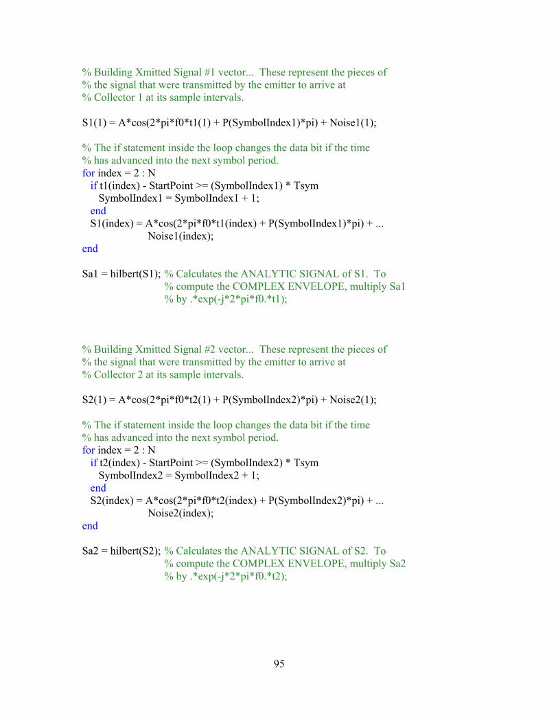
% Building Xmitted Signal #1 vector... These represent the pieces of % the signal that were transmitted by the emitter to arrive at % Collector 1 at its sample intervals. S1(1) = A*cos(2*pi*f0*t1(1) + P(SymbolIndex1)*pi) + Noise1(1); % The if statement inside the loop changes the data bit if the time % has advanced into the next symbol period. for index = 2 : N if t1(index) - StartPoint >= (SymbolIndex1) * Tsym SymbolIndex1 = SymbolIndex1 + 1; end S1(index) = A*cos(2*pi*f0*t1(index) + P(SymbolIndex1)*pi) + ... Noise1(index); end Sa1 = hilbert(S1); % Calculates the ANALYTIC SIGNAL of S1. To % compute the COMPLEX ENVELOPE, multiply Sa1 % by .*exp(-j*2*pi*f0.*t1); % Building Xmitted Signal #2 vector... These represent the pieces of % the signal that were transmitted by the emitter to arrive at % Collector 2 at its sample intervals. S2(1) = A*cos(2*pi*f0*t2(1) + P(SymbolIndex2)*pi) + Noise2(1); % The if statement inside the loop changes the data bit if the time % has advanced into the next symbol period. for index = 2 : N if t2(index) - StartPoint >= (SymbolIndex2) * Tsym SymbolIndex2 = SymbolIndex2 + 1; end S2(index) = A*cos(2*pi*f0*t2(index) + P(SymbolIndex2)*pi) + ... Noise2(index); end Sa2 = hilbert(S2); % Calculates the ANALYTIC SIGNAL of S2. To % compute the COMPLEX ENVELOPE, multiply Sa2 % by .*exp(-j*2*pi*f0.*t2);

95

% This function call simply calculates and displays the expected TDOAs % and FDOAs at the Beginning and End of the collection time. tdoa_fdoa(f0,Pe1(1,:),Pe1(N,:),Pe2(1,:),Pe2(N,:),Ve,Pc1(1,:),...

Pc1(N,:),Vc1,Pc2(1,:),Pc2(N,:),Vc2);

B. “TDOA_FDOA.M” function [TDOA_b, TDOA_e, FDOA_b, FDOA_e] = tdoa_fdoa(f0,Pe1_b,... Pe1_e,Pe2_b,Pe2_e,Ve, Pc1_b,Pc1_e,Vc1,Pc2_b,Pc2_e,Vc2) % ********************************************************************* % TDOA_FDOA is for use with SIG_GEN.m in helping to determine what the % expected TDOA and FDOA are for two signal vectors. % % The function takes the following input arguments: % % f0 -- carrier frequency (assumed to be equal for both signals) % Pe1_b -- [X Y Z] Emitter position WRT Collector 1 at 1st sample % Pe1_e -- [X Y Z] Emitter position WRT Collector 1 at last sample % Pe2_b -- [X Y Z] Emitter position WRT Collector 2 at 1st sample % Pe2_e -- [X Y Z] Emitter position WRT Collector 2 at last sample % Ve -- [X Y Z] Emitter velocity % Pc1_b -- [X Y Z] Collector 1 position at 1st sample % Pc1_e -- [X Y Z] Collector 1 position at last sample % Vc1 -- [X Y Z] Collector 1 velocity % Pc2_b -- [X Y Z] Collector 2 position at 1st sample % Pc2_e -- [X Y Z] Collector 2 postion at last sample % Vc2 -- [X Y Z] Collector 2 velocity % % The output variables are the TDOA at the beginning, TDOA at the % end, FDOA at the beginning, and FDOA at the end, respectively. % Written by: LCDR Joe J. Johnson, USN % Last modified: 26 August 2001 % ********************************************************************* c = 2.997925e8; % Speed of light % The next two lines calculate the Doppler shifts between the emitter % and Collector 1 & Collector 2, respectively, at the BEGINNING of the % collection (i.e., at the instant of the first sample). doppler1_b = f0/c * dot(Ve-Vc1, Pe1_b-Pc1_b) / norm(Pe1_b - Pc1_b); doppler2_b = f0/c * dot(Ve-Vc2, Pe2_b-Pc2_b) / norm(Pe2_b - Pc2_b);

96

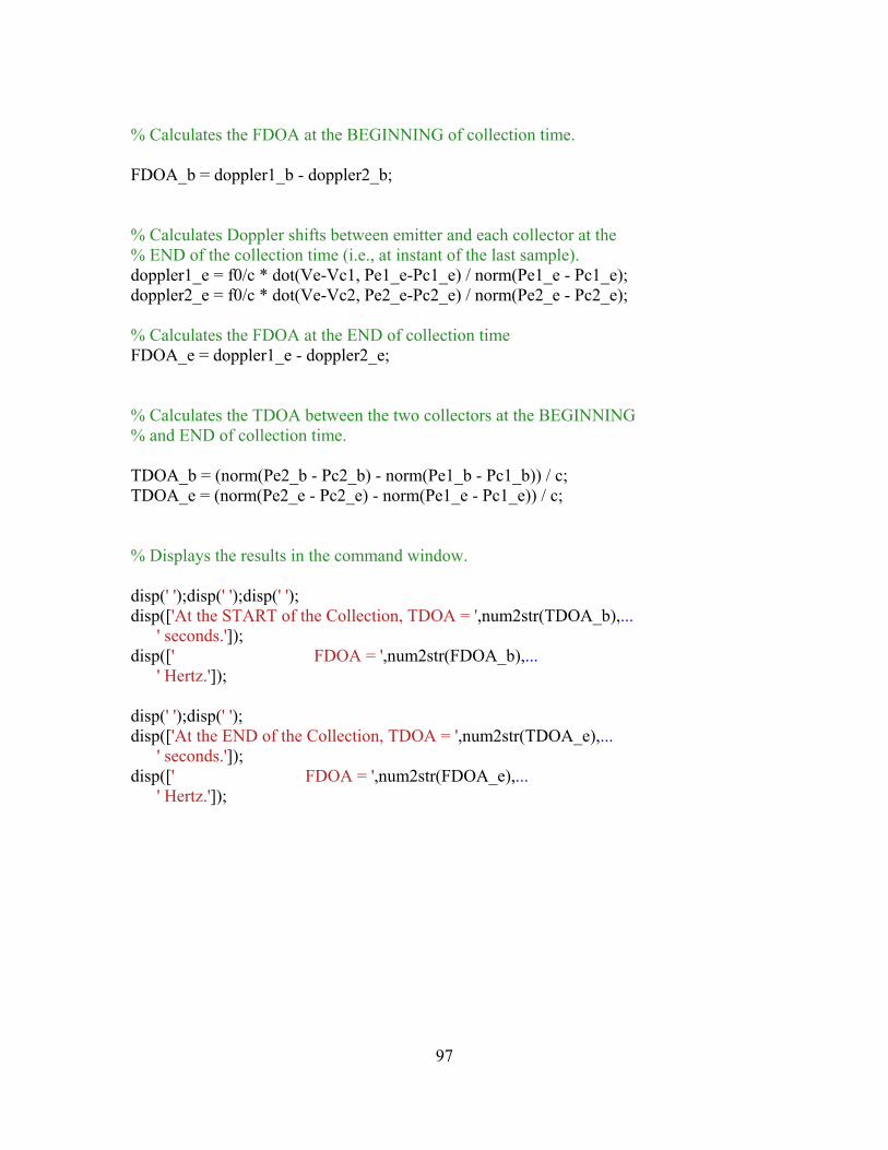
% Calculates the FDOA at the BEGINNING of collection time. FDOA_b = doppler1_b - doppler2_b; % Calculates Doppler shifts between emitter and each collector at the % END of the collection time (i.e., at instant of the last sample). doppler1_e = f0/c * dot(Ve-Vc1, Pe1_e-Pc1_e) / norm(Pe1_e - Pc1_e); doppler2_e = f0/c * dot(Ve-Vc2, Pe2_e-Pc2_e) / norm(Pe2_e - Pc2_e); % Calculates the FDOA at the END of collection time FDOA_e = doppler1_e - doppler2_e; % Calculates the TDOA between the two collectors at the BEGINNING % and END of collection time. TDOA_b = (norm(Pe2_b - Pc2_b) - norm(Pe1_b - Pc1_b)) / c; TDOA_e = (norm(Pe2_e - Pc2_e) - norm(Pe1_e - Pc1_e)) / c; % Displays the results in the command window. disp(' ');disp(' ');disp(' '); disp(['At the START of the Collection, TDOA = ',num2str(TDOA_b),... ' seconds.']); disp([' FDOA = ',num2str(FDOA_b),... ' Hertz.']); disp(' ');disp(' '); disp(['At the END of the Collection, TDOA = ',num2str(TDOA_e),... ' seconds.']); disp([' FDOA = ',num2str(FDOA_e),... ' Hertz.']);

97

THIS PAGE INTENTIONALLY LEFT BLANK

98

LIST OF REFERENCES

[1] S. Stein, “Algorithms for Ambiguity Function Processing,” IEEE Transactions on Acoustics, Speech, and Signal Processing, vol. ASSP-29, no. 3, pp. 588-599, Jun. 1981.

[2] F. Auger, P. Flandrin, O. Lemoine, and P. Goncalves, Time Frequency Toolbox

for MATLAB, http://crttsn.univ-nantes.fr/~auger/tftb.html, Aug. 2001.

[3] R. E. Ziemer and W. H. Tranter, Principles of Communications: Systems, Modulation, and Noise. Houghton-Mifflin, 1976, pp. 94-103.

[4] R. D. Strum and D. E. Kirk, Discrete Systems and Digital Signal Processing. New York: Addison-Wesley, 1988, pp. 384, 430.

[5] W. A. Brown and H. H. Loomis, Jr., “Digital Implementations of Spectral Correlation Analyzers,” IEEE Transactions on Signal Processing, vol. 41, no. 2, pp. 703-720, Feb. 1993.

[6] B. Sklar, Digital Communications: Fundamentals and Applications. Upper Saddle River, NJ: Prentice Hall, 2001, pp. 17-18, 117, 173-174.

[7] H. H. Loomis, Jr., “Geolocation of Electromagnetic Emitters,” Technical Report No. NPS-EC-00-003, Naval Postgraduate School, Monterey, California, Nov. 1999.

[8] R. E. Larson, R. P. Hostetler, and B. H. Edwards, Calculus with Analytic Geometry. Lexington, MA: D. C. Heath and Company, 1990, p. 732.

[9] D. Hanselman and B. Littlefield, Mastering MATLAB: A Comprehensive Tutorial and Reference. Upper Saddle River, NJ: Prentice Hall, 1996, pp. 52-54.

[10] Statistical Signal Processing, Inc., 1909 Jefferson St.; Napa, CA; 94559.

[11] A. Leon-Garcia, Probability and Random Processes for Electrical Engineering. New York: Addison-Wesley, 1994, p. 135.

[12] T. T. Ha, Digital Satellite Communications. New York: McGraw-Hill, 1990.

99 [13] P. Count, private conversation at Naval Postgraduate School, 15 July 2001.

THIS PAGE INTENTIONALLY LEFT BLANK

100

INITIAL DISTRIBUTION LIST 1. Defense Technical Information Center

Fort Belvoir, Virginia

2. Dudley Knox Library Naval Postgraduate School Monterey, California

3. Professor Herschel H. Loomis, Jr. Naval Postgraduate School Monterey, California

4. Professor Ralph D. Hippenstiel Naval Postgraduate School Monterey, California

5. Dr. Michael Price Systeka, Inc. Warrenton, Virginia

6. LCDR(sel) Holly M. Johnson, CEC, USN

Naval Facilities Engineering Command Washington, D.C.

101