thesis breeding season habitat use of conservation

THESIS

BREEDING SEASON HABITAT USE OF CONSERVATION RESERVE PROGRAM (CRP) LAND BY LESSER PRAIRIE-

CHICKENS IN WEST CENTRAL KANSAS

Submitted by

Tamara Leigh Fields

Department of Fishery and Wildlife Biology

In partial fulfillment of the requirements

For the Degree of Master of Science

Colorado State University

Fort Collins, CO

Spring 2004

ii

COLORADO STATE UNIVERSITY

February 5, 2004

WE HEREBY RECOMMEND THE THESIS PREPARED UNDER OUR SUPERVISION BY TAMARA LEIGH FIELDS, ENTITLED BREEDING SEASON HABITAT USE OF CONSERVATION RESERVE PROGRAM (CRP) LAND BY LESSER PRAIRIE CHICKENS IN WEST CENTRAL KANSAS, BE ACCEPTED AS FULFILLING IN PART REQUIREMENTS FOR THE DEGREE OF MASTER

OF SCIENCE.

Committee on Graduate Work

________________________________________

________________________________________

________________________________________ Advisor

________________________________________

Department Head

iii

ABSTRACT OF THESIS

BREEDING SEASON HABITAT USE OF CONSERVATION RESERVE PROGRAM (CRP) LAND BY LESSER PRAIRIE-CHICKENS IN WEST

CENTRAL KANSAS

Lesser prairie-chicken (Tympanuchus pallidicinctus) populations have drastically

declined throughout their range since the 1800�s. In Kansas, counts of leks and

individual birds indicate that populations have experienced significant declines since

1964. The primary cause of range-wide and statewide declines has been deterioration

of suitable habitats. Recently, populations of lesser prairie-chickens have expanded

northward and westward in Kansas. The range expansion has been attributed to an

increase in CRP (Conservation Reserve Program) lands. This study assessed the

importance of CRP and the interseeding of forbs in CRP to lesser prairie-chickens.

Invertebrate sampling was conducted in June, July, and August 2001 to

determine whether interseeding increased invertebrate biomass and diversity.

Sweepnet samples were collected on five grassland CRP fields that were successfully

interseeded with alfalfa and sweet clover in alternating strips on 50% of the field. Total

invertebrate biomass and diversity were greater on interseeded CRP plots compared to

grass CRP plots. There was no evidence of a treatment effect on orthoptera,

lepidoptera larvae, hemiptera, hymenoptera, and coleoptera biomass. However,

differences in orthoptera biomass between grass and interseeded plots suggest that the

majority of the treatment effect on total biomass could be attributed to this order.

Greater total invertebrate biomass and count diversity was attributed to the abundance

of forbs found within interseeded fields.

4

Seventy-one female lesser and greater prairie-chickens (Tymanuchus cupido)

were equipped with transmitters during the 2002 and 2003 breeding seasons to monitor

habitat selection and survival. Fields were classified into five habitat types: native

rangelands, croplands, grassland CRP (GCRP), interseeded CRP (ICRP), and forb CRP

(FCRP). Habitat selection of pre- and post-nesting hens (n = 68), nesting hens (n = 60),

and hens with broods (n = 27) was determined by comparing use to habitat availability

within the southwest quarter of Gove County. Hens used cropland less than expected

and ICRP more than expected. Nesting hens used FCRP, rangeland, and cropland less

than expected and GCRP and ICRP more than expected. Greater use of ICRP and

GCRP fields was attributed to the abundance of invertebrates and cover provided by

ICRP and GCRP, respectively. Lastly, hens with broods used cropland less than

expected and demonstrated no habitat selection for any habitat types. The lack of

selection by hens with broods is most likely a product of small sample sizes in my study.

Lack of selection was also a product of high rangeland brood use and the high

availability of this habitat type. Additionally, habitat type was not considered the most

important determinant of a brood�s location. Instead, broods were frequently located in

heterogeneous fields characterized by grassy cover interspersed with an abundance of

forbs.

A number of nest and brood statistics were computed as an index of reproductive

success. Nesting rate was 89.7%, hatchability was 76.5%, renesting rate was 19.1%,

and mean clutch size was 11.2 eggs. Apparent brood success (> 1 chick survived) to 14

days was 65.6%, and 53.8% of these broods survived to 60 days. Only 28% of tracked

broods survived from hatch to 60 days post-hatch. In addition to complete brood loss,

the number of chicks per brood declined from 9.6 (SE = 0.7) at hatch to 5.0 (SE = 3.7)

5

60 days post-hatch. Mean recruitment at 60 days post-hatch was 0.59 chicks per hen

(SE = 0.10), overall chick survival for pre-fledge broods was 0.433 (SE = 0.03), overall

chick survival for post-fledge broods was 0.372 (SE = 0.05), and overall chick survival

over the entire period was 0.161 (SE = 0.02).

Survival rate of hens, nests, and broods were estimated using Program MARK.

The known fate data type was used to model weekly survival probabilities of hens as a

function of eight time-specific and individual covariates. The same data type was used

to evaluate the effects of 13 sources of variation on the daily nest survival probabilities.

To model daily brood survival probabilities as a function of 14 sources of variation, the

nest survival data type available in Program MARK was used. All candidate models

within each survival analysis were ranked based on a small sample Akaike�s Information

Criteria (AICc). In addition to evaluating the effects of different sources of variation, the

best model within each analysis was used to estimate model-conditional survival

estimates.

The level of model selection uncertainty within the hen survival analysis indicates

that none of the models approximated weekly hen survival probabilities well. However,

the best model suggested a positive association between survival and weekly

precipitation. The probability of a female prairie chicken surviving the breeding season

was 0.62 (SE = 0.14) and 0.66 (SE = 0.12) in 2002 and 2003, respectively. Daily

survival probabilities of nests were a function of a quadratic time trend, nest age, and

temperature. Daily nest survival probabilities declined as the season progressed. Nest

age and temperature were also negatively correlated with daily nest survival. The

probability of a nest surviving from May 10 to June 1 was 0.70. Daily brood survival

probabilities were a function of a quadratic time trend, brood age, hen age, forb

6

composition and precipitation events. Daily brood survival declined as the season

progressed. Brood age and forb composition were positively associated with daily

survival, whereas precipitation was negatively correlated with daily survival. Broods

tended by adult hens had higher daily survival probabilities than broods of juvenile hens.

The probability of a brood surviving from June 1 to July 30 (hatch to 60 days post-hatch)

was 0.52 and 0.06 for a brood reared by an adult and juvenile, respectively.

The habitat selection analyses indicate that ICRP and GCRP may be beneficial

to prairie chickens during the breeding season. Although there was no evidence that

hen, nest, and brood survival were a function of habitat, the long-term benefit of CRP

was evident. From field observations it was apparent that CRP may be allowing these

birds to persist in dry years. In contrast, rangeland may be adequate when drought and

the compounding effects of grazing do not decrease cover and food sources.

Tamara Leigh Fields Fishery and Wildlife Biology Department

Colorado State University Fort Collins, CO 80523 Spring 2004

7

ACKNOWLEDGEMENTS

I would like to extend a special thanks to my advisor, Dr. Gary White, Professor

of Fishery and Wildlife Biology, Colorado State University. Gary�s guidance throughout

my research was an unquestionable asset to my project. I would also like to extend a

special thanks to Wendell Gilgert, State Biologist, Natural Resource Conservation

Service. Wendell shared his extensive knowledge of wildlife biology with me and made

this project possible by providing financial support. Another special thanks to Randy D.

Rodgers, Biologist, Kansas Wildlife and Parks, who shared his knowledge of prairie

grouse and rangeland ecosystems.

I am genuinely grateful for the help I received from my committee members, Dr.

Gary C. White, Dr. Wayne Leininger, Professor of Forest, Rangeland, and Watershed

Stewardship, Colorado State University, and Dr. Julie Savidge, Associate Professor of

Fishery and Wildlife Biology, Colorado State University, for their comments and advice

on my proposal, research, and thesis.

I sincerely appreciate the help of Leah Ricke, District Conservationist, Gove

County, Kansas for providing pertinent landowner and land use information. I am deeply

indebted to Christian Hagen and Jim Pitman, Graduate Students, Kansas State

University, for their invaluable guidance in the field. I am especially appreciative of Dr.

Boris Kondratieff, Professor of Bioagricultural Sciences and Pest Management, Colorado

State Univeristy, for his expert advice on insect ecology and Dr. Phil Chapman,

Associate Professor of Statistics, Colorado State University, for his statistical guidance.

I would also like to thank the technicians, Jenny Dehn, Jenny Biggs, Elizabeth Doxon,

and Jennifer Courtemanche, for their unwavering dedication to this research.

8

TABLE OF CONTENTS

ABSTRACT OF THESIS…..………………………………………………...…………...……iii

CHAPTER 1: INVERTEBRATE BIOMASS AND DIVERSITY IN INTERSEEDED AND GRASSLAND

CRP……..…………………………………………………………………….…1

INTRODUCTION��.��..1

STUDY AREA��.��2

METHODS�...��...3

RESULTS��.�..4

DISCUSSION��.��5

MANAGEMENT IMPLICATIONS��7

LITERATURE CITED��.��...8

TABLES��.��11

FIGURES��.��.12

CHAPTER 2: BREEDING SEASON HABITAT USE AND SELECTION BY

PRAIRIE CHICKEN

HENS��.��15

INTRODUCTION��.��...�.15

STUDY AREA��.��.18

METHODS�...��.20

Locating and Monitoring Hens��..20

Vegetation Sampling��..21

Habitat Use Analyses��.21

9

Habitat Selection Analyses�.��.��.24

RESULTS��.�25

Hen Habitat Analyses��25

Nest Habitat Analyses��.��..26

Brood Habitat Analyses��.27

DISCUSSION��.��..28

MANAGEMENT IMPLICATIONS��..34

LITERATURE CITED��.��.36

TABLES��.��41

FIGURES��.��.51

CHAPTER 3: SURVIVAL OF PRAIRIE CHICKEN HENS, NESTS, AND

BROODS��..��..��..��

��59

INTRODUCTION��.��...�.59

METHODS�...��.62

Locating and Monitoring Hens...��..62

Vegetation Sampling��..63

Nesting Statistics�..��..64

Brood Statistics...��65

Survival Analyses��..��.65

Hens��.67

Nests��68

Broods��.71

Annual Rate of Population Growth��.��..��..75

10

RESULTS��.�76

Nesting Statistics�..��..77

Brood Statistics...��77

Survival Analyses��..��.78

Hens��78

Nests��79

Broods��.80

Annual Rate of Population Growth�..��..��.82

DISCUSSION��.��..83

MANAGEMENT IMPLICATIONS��..93

LITERATURE CITED��.��.95

TABLES��.�.��103

FIGURES��..��.118

11

CHAPTER 1:

INVERTEBRATE BIOMASS AND DIVERSITY IN INTERSEEDED AND GRASSLAND CRP

INTRODUCTION

In contrast to range-wide declines, there has been a recent expansion of lesser

prairie-chickens (Tympanuches pallidicinctus) northward and westward in Kansas. This

expansion coincided with the designation of certain counties as Pheasant Initiative

Priority Areas and its� influence on Conservation Reserve Program (CRP) management.

In particular, the expansion has been attributed to an increase in prairie chicken

reproductive success resulting from forb interseeding on grass CRP fields (R. Rodgers,

Kansas Wildlife and Parks, personal communication).

The reproductive period (summer) of lesser prairie-chickens has been suggested

as the most critical period limiting lesser prairie-chicken populations (Hamerstrom et al.

1957, Kirsch et al. 1974). During this period, invertebrates are the primary dietary

component of hens and chicks (Schwilling 1955, Jones 1963, Davis et al. 1980, Doerr

and Guthery 1983, Applegate and Riley 1998). Several studies have found that

grasshoppers (orthoptera) are the most abundant invertebrates in the diet of lesser

prairie-chicken chicks. In addition, treehoppers (hemiptera), ants (hymenoptera), wasps

(hymenoptera), and beetles (coleoptera) have been found to be important secondary

components (Jones et al. 1963, Davis et al. 1980, Doerr and Guthery 1983, Jamison

2000). Research has revealed that vegetation structure and composition are important

predictors of invertebrate abundance and diversity (Southwood and Cross 1969). In

12

particular, forbs provide a preferred substrate for many invertebrates (Jones 1963,

Southwood and Cross 1969, Burger et al. 1993, Jamison 2000).

13

The Conservation Reserve Program (CRP) was initiated in 1986 in Gove County,

Kansas by the 1985 Farm Bill. It is currently administered by the Natural Resource

Conservation Service (NRCS). This program requires the seeding of highly erodible

agricultural fields with native grass species. Prior to 1997, CRP fields consisted of

primarily grass species (GCRP). In 1997, interseeding of CRP fields, as a management

strategy to improve wildlife habitat, was implemented (ICRP). Each designated grass

CRP field was interseeded with forbs in strips on 50% of the field by NRCS or Kansas

Wildlife and Parks (KWP). The use of forbs within the grass seed mixtures on newly

enrolled CRP was initiated in 1998 (FCRP).

Due to the varying response of invertebrates to vegetation structure and

composition and the importance of invertebrates to lesser prairie-chicken populations, it

is essential that interseeded CRP be evaluated. This study was conducted to ascertain

whether interseeding increases insect biomass and diversity on CRP fields. I

hypothesized that interseeded CRP would have greater invertebrate biomass and

diversity than grass CRP fields.

STUDY AREA

Fieldwork was conducted during the summer of 2001 in southwest Gove County,

Kansas. The total land area in Gove County is 277,100 ha, which includes 146,800 ha

of cropland and rangeland and 10,750 ha of CRP. Parent material in this area is

classified as sedimentary. Soils primarily consist of Ulysses-Elkader-Manvel

associations and are characterized as moderately steep silt loam soils with medium

textured subsoils and rock outcrops on uplands (Angell et al. 1978). The climate is

semi-arid due to its location within the rain shadow of the Rockies. Temperatures range

from –23 to 41 C and annual precipitation ranges from 51 to 61 cm with 75% of

precipitation occurring between April and September. Elevation ranges from 700 to 915

14

m. Topography is gently undulating to rolling (Angell et al. 1978).

As mentioned previously, CRP was initiated in 1986 in Gove County. Little

bluestem, sideoats grama, big bluestem, blue grama, buffalograss, switchgrass, and

western wheatgrass were typical grass species seeded on CRP. Indiangrass

(Sorghastrum nutans) was also included in a small percentage of CRP seed mixtures.

The use of forbs within the grass seed mixtures began with the new Sign-up 16 and

included Maximillian sunflower (Helianthus maximiliani), purple prairie clover

(Petalostemon purpureum), prairie coneflower (Ratibida columnifera) (in Sign-up 18 and

20 only), and Illinois bundleflower (Desmanthus illinoensis). In 1997, interseeding, as a

management strategy to improve wildlife habitat, was implemented on old Sign-up 16,

18, and 20 fields. Fifty percent of each field was interseeded using grazer alfalfa, white

(Melilotus alba) or yellow sweet clover (Melilotus officinalis). Some established CRP

(CRP prior to and including Sign-up 15) was also interseeded by the Kansas Wildlife and

Parks (KWP). KWP interseeded with grazer alfalfa, Maximillian sunflower, Illinois

bundlflower, purple prairie clover, partridge pea (Chamaecrista fasciculata), and prairie

coneflower. Fields were baled, mowed, burned, or tilled in alternate strips on at least

51% of the established grassland CRP prior to interseeding. Seeding was performed by

drilling the seed 0.64-1.3 cm into the soil (L. Ricke, Natural Resource Conservation

Service, personal communication).

METHODS

Invertebrates were sampled on five grassland CRP fields successfully

interseeded with grazer alfalfa and sweet clover on 50% of each field. Fields

interseeded in 1998 and 1999 were selected if interseeding success exceeded 75%.

Three samples were collected during June, July, and August in the grass CRP section

and in the paired interseeded section of each field (treatment). These months

15

encompass the lesser prairie-chicken brood-rearing season. Ten 1-m2 sample plots were

selected within each section >25 m from the edge. One hundred sweeps with a

sweepnet were taken within each plot during each month. Samples were taken during

mid-day when diurnal insects concentrate at the base of the vegetation and are the most

available for collection (Manley et al. 1994). Sampling was avoided during rain or winds

exceeding 30 km/hr.

The contents of the sweepnet and collection cups were emptied into labeled

plastic bags and placed on ice. Insects were sorted, identified to order, counted, and

weighed. Biomass of each order, counts of each order, and total biomass was recorded

for each sample. Diversity of each sample was calculated using the Shannon-Weiner

biodiversity index (Pielou 1975):

( )∑=

=n

iii ppH

1

ln'

where H’ represents the diversity index, n is the number of orders, pi represents the

proportion of each order compared to the total, and ln (pi) is the natural logarithm of pi.

Total invertebrate biomass, biomass of each order, count diversity, and biomass

diversity were averaged across control and treatment plots within each month and

analyzed using an autoregressive repeated measures analysis (Proc Mixed in SAS)

(SAS 1989). The treatment was blocked by field, with field considered a random effect.

A treatment effect, a month effect, and a treatment by month interaction were included to

determine the difference between treatments over time. Estimates of the overall

treatment effect were calculated using least square means.

RESULTS

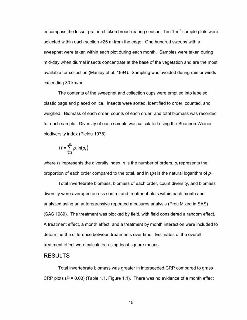
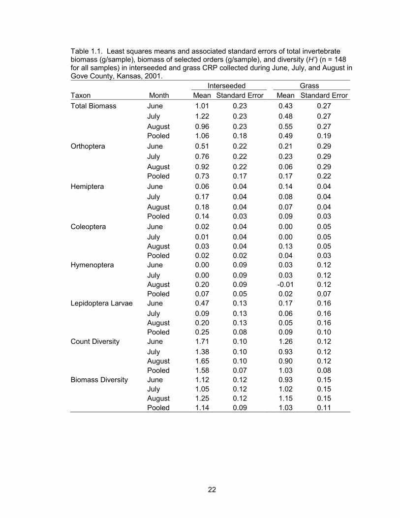
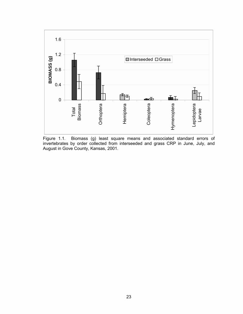
Total invertebrate biomass was greater in interseeded CRP compared to grass

CRP plots (P = 0.03) (Table 1.1, Figure 1.1). There was no evidence of a month effect

16

or a month by treatment interaction effect (Table 1.1). There was no evidence of a

treatment effect on orthoptera, hemiptera, hymenoptera, coleoptera, or lepidoptera

larvae (Table 1.1). However, differences in orthoptera biomass between grass and

interseeded plots suggest that the majority of the treatment effect on total biomass could

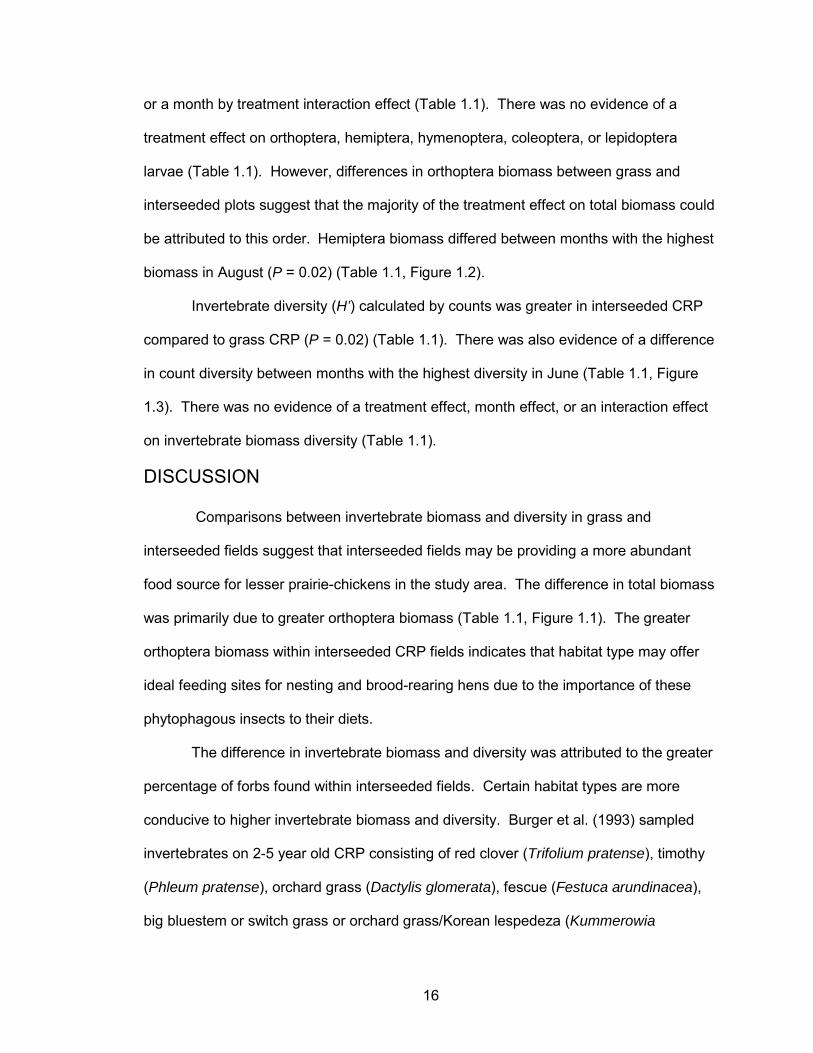
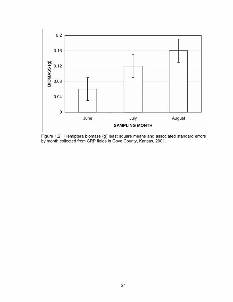
be attributed to this order. Hemiptera biomass differed between months with the highest

biomass in August (P = 0.02) (Table 1.1, Figure 1.2).

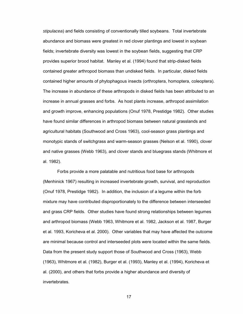
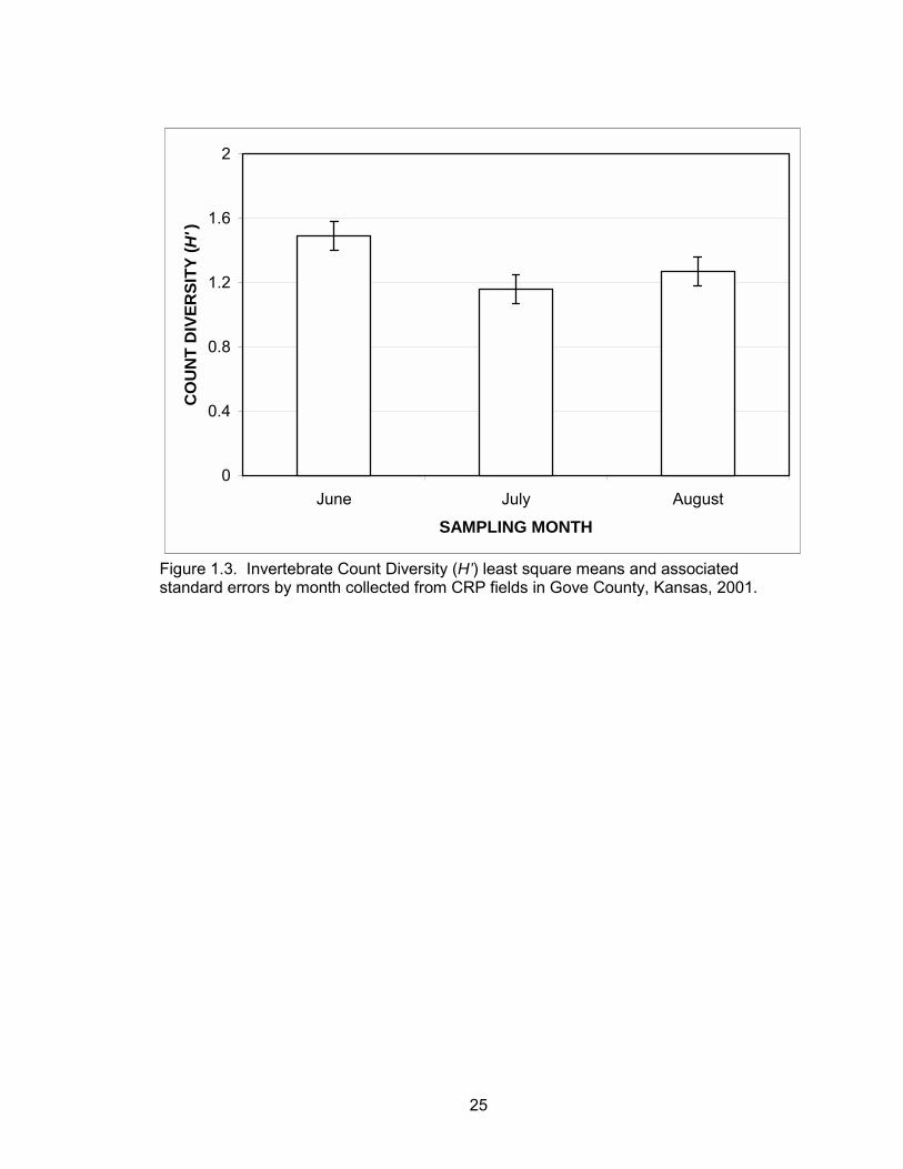
Invertebrate diversity (H’) calculated by counts was greater in interseeded CRP

compared to grass CRP (P = 0.02) (Table 1.1). There was also evidence of a difference

in count diversity between months with the highest diversity in June (Table 1.1, Figure

1.3). There was no evidence of a treatment effect, month effect, or an interaction effect

on invertebrate biomass diversity (Table 1.1).

DISCUSSION

Comparisons between invertebrate biomass and diversity in grass and

interseeded fields suggest that interseeded fields may be providing a more abundant

food source for lesser prairie-chickens in the study area. The difference in total biomass

was primarily due to greater orthoptera biomass (Table 1.1, Figure 1.1). The greater

orthoptera biomass within interseeded CRP fields indicates that habitat type may offer

ideal feeding sites for nesting and brood-rearing hens due to the importance of these

phytophagous insects to their diets.

The difference in invertebrate biomass and diversity was attributed to the greater

percentage of forbs found within interseeded fields. Certain habitat types are more

conducive to higher invertebrate biomass and diversity. Burger et al. (1993) sampled

invertebrates on 2-5 year old CRP consisting of red clover (Trifolium pratense), timothy

(Phleum pratense), orchard grass (Dactylis glomerata), fescue (Festuca arundinacea),

big bluestem or switch grass or orchard grass/Korean lespedeza (Kummerowia

17

stipulacea) and fields consisting of conventionally tilled soybeans. Total invertebrate

abundance and biomass were greatest in red clover plantings and lowest in soybean

fields; invertebrate diversity was lowest in the soybean fields, suggesting that CRP

provides superior brood habitat. Manley et al. (1994) found that strip-disked fields

contained greater arthropod biomass than undisked fields. In particular, disked fields

contained higher amounts of phytophagous insects (orthroptera, homoptera, coleoptera).

The increase in abundance of these arthropods in disked fields has been attributed to an

increase in annual grasses and forbs. As host plants increase, arthropod assimilation

and growth improve, enhancing populations (Onuf 1978, Prestidge 1982). Other studies

have found similar differences in arthropod biomass between natural grasslands and

agricultural habitats (Southwood and Cross 1963), cool-season grass plantings and

monotypic stands of switchgrass and warm-season grasses (Nelson et al. 1990), clover

and native grasses (Webb 1963), and clover stands and bluegrass stands (Whitmore et

al. 1982).

Forbs provide a more palatable and nutritious food base for arthropods

(Menhinick 1967) resulting in increased invertebrate growth, survival, and reproduction

(Onuf 1978, Prestidge 1982). In addition, the inclusion of a legume within the forb

mixture may have contributed disproportionately to the difference between interseeded

and grass CRP fields. Other studies have found strong relationships between legumes

and arthropod biomass (Webb 1963, Whitmore et al. 1982, Jackson et al. 1987, Burger

et al. 1993, Koricheva et al. 2000). Other variables that may have affected the outcome

are minimal because control and interseeded plots were located within the same fields.

Data from the present study support those of Southwood and Cross (1963), Webb

(1963), Whitmore et al. (1982), Burger et al. (1993), Manley et al. (1994), Koricheva et

al. (2000), and others that forbs provide a higher abundance and diversity of

invertebrates.

18

There was no difference in biomass for hemiptera, hymenoptera, coleoptera, or

for any of the other invertebrate orders encountered in the present study. In contrast to

my findings, a number of other studies found that hemiptera, hymenoptera, and

coleoptera increased with forbs (Manley et al. 1994, Koricheva et al. 2000, Symstad et

al. 2000). The difference between the present study and others may be due to

limitations resulting from only identifying to order and/or collection methods. Koricheva

et al. (2000) found that response of hemiptera to increased plant diversity depended on

the family. In their study, leafhoppers responded to above ground plant biomass and

percent cover, whereas wingless aphids responded to number of plant functional groups.

Varying responses were attributed to a difference in life history strategy. Coleoptera and

hymenoptera were probably misrepresented in the present study because sweepnet

sampling collects invertebrates that dwell on the vegetation, whereas other sampling

techniques are more efficient at collecting ground dwelling insects and insects at the

base of the vegetation (Wilson et al. 1993). Lastly, failure to quantify vegetation

variables within the sample plots may have influenced the strength of the treatment

effect. There was one control section that contained a substantial amount of forbs,

which may have diluted the differences between control and interseeded fields.

MANAGEMENT IMPLICATIONS

Management techniques that increase forb abundance may be beneficial to

lesser prairie-chicken populations by increasing invertebrate populations. Interseeding

is only one of several approaches to creating patches of forbs on CRP. Strip disking,

prescription grazing, mowing, and burning are other alternatives that are compatible with

CRP management (Hurst 1972, Buckner and Landers 1979, Landers and Mueller 1986,

Manley et al. 1994, Bidwell et al. 2002). Litton et al. (1994) recommended strip-disking

at depths of 7 to 15 cm during March. Bidwell et al. (2002) recommended burning 20-30

19

percent of the field each year during late summer, fall, or winter with a 3 to 5 year

interval. This would allow maintenance of nesting cover, while providing early

successional patches for foraging. Any management plan aimed at providing habitat for

lesser prairie-chickens should maintain the prairie in mid to late successional stages for

cover, while providing early stages for foraging. Lastly, management techniques that

manipulate plant species richness, diversity, biomass, cover, and the number of plant

functional groups may also result in greater invertebrate biomass.

LITERATURE CITED

Angell, R. C., C. M. Call, and L. D. Linnell. 1978. Soil Survey of Gove County, Kansas. United States Department of Agriculture, Natural Resource Conservation Service.

Applegate, R. D., and T. Z. Riley. 1998. Lesser prairie-chicken management.

Rangelands 20:13-16. Bidwell, T. G, S. D. Fuhlendorf, B. Gillen, S. Harmon, R. Horton, R. D. Rodgers, S.

Sherrod, D. Weidenfeld, and D. Wolfe. 2002. Ecology and management of the lesser prairie-chicken in Oklahoma. Oklahoma Cooperative Extensive Service, Stillwater, Oklahoma. USA.

Buckner, J. L., and J. L. Landers. 1979. Fire and soil disturbance effects on herbaceous

food plants and seed supplies. Journal of Wildlife Management 43:807-811. Burger, L. W. Jr., E. W. Kurzejeski, T. V. Dailey, and M. R. Ryan. 1993. Relative

invertebrate abundance and biomass in Conservation Reserve Program plantings in Northern Missouri. Pages 102-108 in K. E. Church and T. V. Dailey, editors. Quail III: national quail symposium. Kansas Department of Wildlife and Parks, Pratt, Kansas, USA.

Davis, C. A., T. Z. Riley, R. A. Smith, and M. J. Wisdom. 1980. Spring-summer food of

lesser prairie chicken in New Mexico. Pages 75-80 in P. A. Vohs, Jr. and F. L Knopf, editors. Proceedings of the Prairie Grouse Symposium. Oklahoma State University, Stillwater, OK, USA.

Doerr, T. B., and F. S. Guthery. 1983. Food selection by lesser prairie chickens in

northwest Texas. Southwest Naturalist 28:381-383. Hamerstrom, F. N., Jr., O. E. Mattson, and F. Hamerstrom. 1957. Guide to prairie

chicken management. Technical Wildlife Bulletin Publication 5. Wisconsin Conservation Department, Madison, Wisconsin, USA.

Hurst, G. A. 1972. Insects and bobwhite quail brood management. Pages 65-82 in J.

20

A. Morrison and L. C. Lewis, editors. Proceedings of the First National Bobwhite Quail Symposium, Oklahoma State University, Stillwater, Oklahoma, USA.

Jackson, J. R., G. A. Hurst, and E. A. Gluesing. 1987. Abundance and selection of

invertebrates by northern bobwhite chicks. Proceedings of the Annual Conference of the Southeastern Association of Fish and Wildlife Agencies 41:303-310.

Jamison, B. E. 2000. Lesser prairie chicken chick survival, adult survival, and habitat

selection and movements of females in fragmented rangelands of southwestern Kansas. Thesis, Kansas State University, Manhattan, Kansas, USA.

Jones, R. E. 1963. Identification and analysis of lesser and greater prairie chicken

habitat. Journal of Wildlife Management 27:757-778. Kirsch, L. M. 1974. Habitat management considerations for prairie chickens. Wildlife

Society Bulletin 2:125-129. Koricheva, J., C. P. H. Mulder, B. Schmid, J. Joshi, and K. Huss-Danell. 2000.

Numerical responses of different trophic groups of invertebrates to manipulations of plant diversity in grasslands. Oecologia 125:271-282.

Landers, J. L., and B. S. Mueller. 1986. Bobwhite quail management: a habitat

approach. Publication 4. Tall Timbers Research Station, Tallahassee, Florida, USA.

Litton, G., R. L. West, D. F. Dvorak, and G. T. Miller. 1994. The lesser prairie chicken

and its management in Texas. Federal Aid Report 33. Texas Parks and Wildlife, Austin, Texas, USA.

Manley, S. W., R. S. Fuller, J. M. Lee, and L. A. Brennan. 1994. Arthropod response to

strip disking in old fields managed for northern bobwhites. Proceedings of the Annual Conference of the Southeastern Association of Fish and Wildlife Agencies 48:227-235.

Menhinick, E. F. 1967. Structure, stability, and energy flow in plants and arthropods in a

sericia lespedeza stand. Ecological Monographs 37:255-272. Nelson, D. R., R. O. Kimmel, and M. J. Frydendall. 1990. Ring-necked pheasant and

gray partridge brood habitat in roadsides and managed grasslands. Pages 103-119 in K. E. Church and S. J. Brady, editors. Perdix V: gray partridge and ring-necked pheasant workshop. Kansas Department of Wildlife and Parks, Emporia, Kansas, USA.

Onuf, C. 1978. Nutritive value as a factor in plant-insect interactions with an emphasis

on field studies. Pages 85-96 in G. G. Montgomery editor. The ecology of arboreal folivores. Smithsonian Institute Press, Washington D.C, USA.

Pielou, E. C. 1975. Ecological Diversity. John Wiley & Sons, New York, New York,

USA.

21

Prestidge, R. A. 1982. Instar duration, adult consumption, oviposition, and nitrogen utilization efficiencies of leafhoppers feeding on different quality food (auchenorrhyncha, homoptera). Ecological Entomology 7:91-101.

SAS Institute Inc., 1989. SAS/STAT User�s Guide, Version 6, 4th Edition, Volume 2.

Cary, North Carolina. 846pp. Schwilling, M. 1955. Study of lesser prairie chicken in southwest Kansas. Kansas Fish

and Game 12:10-12. Southwood, T. R. E., and D. J. Cross. 1963. The Ecology of the Partridge III. Breeding

success and the abundance of insects in natural habitats. Journal of Animal Ecology 38:497-507.

Symstad, A. J., E. Siemann, and J. Haarstad. 2000. An experimental test of the effect

of plant functional group diversity on arthropod diversity. Oikos 89:243-253. Webb, L. G. 1963. Utilization of domestic crops by deer and wild turkeys with notes on

insects inhabiting crops. Proceedings of the Annual Conference of the Southeastern Association of Game and Fish Commission 17:92-100.

Whitmore, R. W., K. P. Pruess, and R. E. Gold. 1986. Insect food selection by 2-week-

old ring-necked pheasant chicks. Journal of Wildife Management 50:223-228. Wilson, S. W., J. L. Smith, and A. H. Purcell III. 1993. An inexpensive vacuum collector

for insect sampling. Entomological News 104: 203-208.

22

Table 1.1. Least squares means and associated standard errors of total invertebrate biomass (g/sample), biomass of selected orders (g/sample), and diversity (H’) (n = 148 for all samples) in interseeded and grass CRP collected during June, July, and August in Gove County, Kansas, 2001. Interseeded Grass Taxon Month Mean Standard Error Mean Standard ErrorTotal Biomass June 1.01 0.23 0.43 0.27 July 1.22 0.23 0.48 0.27 August 0.96 0.23 0.55 0.27 Pooled 1.06 0.18 0.49 0.19 Orthoptera June 0.51 0.22 0.21 0.29 July 0.76 0.22 0.23 0.29 August 0.92 0.22 0.06 0.29 Pooled 0.73 0.17 0.17 0.22 Hemiptera June 0.06 0.04 0.14 0.04 July 0.17 0.04 0.08 0.04 August 0.18 0.04 0.07 0.04 Pooled 0.14 0.03 0.09 0.03 Coleoptera June 0.02 0.04 0.00 0.05 July 0.01 0.04 0.00 0.05 August 0.03 0.04 0.13 0.05 Pooled 0.02 0.02 0.04 0.03 Hymenoptera June 0.00 0.09 0.03 0.12 July 0.00 0.09 0.03 0.12 August 0.20 0.09 -0.01 0.12 Pooled 0.07 0.05 0.02 0.07 Lepidoptera Larvae June 0.47 0.13 0.17 0.16 July 0.09 0.13 0.06 0.16 August 0.20 0.13 0.05 0.16 Pooled 0.25 0.08 0.09 0.10 Count Diversity June 1.71 0.10 1.26 0.12 July 1.38 0.10 0.93 0.12 August 1.65 0.10 0.90 0.12 Pooled 1.58 0.07 1.03 0.08 Biomass Diversity June 1.12 0.12 0.93 0.15 July 1.05 0.12 1.02 0.15 August 1.25 0.12 1.15 0.15 Pooled 1.14 0.09 1.03 0.11

23

0

0.4

0.8

1.2

1.6

Tota

lB

iom

ass

Orth

opte

ra

Hem

ipte

ra

Col

eopt

era

Hym

enop

tera

Lepi

dopt

era

Larv

ae

BIO

MA

SS (g

)

Interseeded Grass

Figure 1.1. Biomass (g) least square means and associated standard errors of invertebrates by order collected from interseeded and grass CRP in June, July, and August in Gove County, Kansas, 2001.

24

0

0.04

0.08

0.12

0.16

0.2

June July August

SAMPLING MONTH

BIO

MA

SS (g

)

Figure 1.2. Hemiptera biomass (g) least square means and associated standard errors by month collected from CRP fields in Gove County, Kansas, 2001.

25

0

0.4

0.8

1.2

1.6

2

June July August

SAMPLING MONTH

CO

UN

T D

IVER

SITY

( H')

Figure 1.3. Invertebrate Count Diversity (H’) least square means and associated standard errors by month collected from CRP fields in Gove County, Kansas, 2001.

26

CHAPTER 2:

BREEDING SEASON HABITAT USE AND SELECTION BY PRAIRIE CHICKEN HENS

INTRODUCTION

The lesser prairie-chicken (Tympanuchus pallidicinctus) has the smallest and

most restricted range of any North American grouse species (Giesen 1998). Remnant

populations of lesser prairie-chickens exist within southwestern Kansas, southeastern

Colorado, northern Texas, western Oklahoma, and eastern New Mexico (Huakos and

Smith 1989). Habitats in Colorado, Kansas, and portions of Oklahoma consist mainly of

sand-sage prairie intermixed with short-grass prairie (Applegate and Riley 1998).

Livestock grazing within this habitat type has converted a shortgrass prairie to

shortgrass disclimax with a substantial portion of climax species replaced by weeds

(Hoffman 1963). In contrast to the sand sagebrush communities, habitat in New Mexico,

Texas, and Oklahoma is comprised of sand-shinnery oak grasslands (Applegate and

Riley 1998).

Within their home range, lesser prairie-chickens require a juxtaposition of habitat

types. Lekking grounds, nesting, brood-rearing, and fall/winter habitats are all pertinent

habitat components of this mosaic. All of these components are typically concentrated

within 4.8 km of their lekking grounds, and birds may spend their entire lives within this

area (Giesen 1994, Riley et al. 1994, Applegate and Riley 1998). Among these habitat

types, nesting and brood-rearing habitats are considered most limiting for prairie-chicken

populations (Hamerstrom et al. 1957, Kirsch 1974).

Nesting habitat must provide adequate concealment from predators and

protection from wind, temperature extremes, and solar radiation (Riley et al. 1992). As a

27

result, hens typically select nest sites surrounded by tall dense residual cover and a high

grass composition (Riley 1978, Candelaria 1979, Davis et al. 1979, Wisdom 1980,

Wilson 1982, Riley et al. 1992). In particular, grasses, such as sand bluestem

(Andropogon hallii) and little bluestem (Andropogon scoparius), and shrubs, such as

sand sagebrush (Artemisia filifolia) and shinnery oak (Quercus havardii), have been

identified as important nest site vegetation components (Wilson 1982, Huakos and Smith

1989). Nest sites are also commonly characterized by a considerable portion of litter

and bare ground within 3 m of the nest (Jones 1963, Riley 1978, Sell 1979, Davis et al.

1979, Wisdom 1980, Giesen 1994).

Successful brood-rearing habitat must provide protection from extreme weather,

protection from predators, ample food, and allow adequate brood mobility (Jones 1963,

Ahlborn 1980, Riley and Davis 1993). Because of these requirements, habitat that is

composed of grasses and shrubs along with an abundance of perennial and annual

forbs has been considered ideal brood-rearing habitat (Jones 1963, Candelaria 1979,

Sell 1979, Ahlborn 1980, Huakos and Smith 1989, Riley and Davis 1993). Shrubs and

grasses along with topography provide a microclimate favorable to broods during the

high temperatures of the summer months (Ahlborn 1980). Forbs provide a preferred

substrate for many invertebrates (Jones 1963, Southwood and Cross 1969, Burger et al.

1993, Jamison 2000), which are the primary dietary component of chicks (Jones 1963,

Davis et al. 1980, Doerr and Guthery 1983, Applegate and Riley 1998, Jamison 2000).

Broods also require a substantial amount of bare ground to enable movement through

the vegetation (Riley and Davis 1993).

In contrast to range-wide declines, lesser prairie-chicken populations have

recently expanded northward and westward into Gove County, Kansas. In addition to an

expansion of lesser prairie-chickens into the area, greater prairie-chickens

(Tympanuchus cupido) currently inhabit the area. The increase in prairie chickens has

28

been attributed to the influence of Pheasant Initiative Priority Area designation on

Conservation Reserve Program (CRP) management. In particular, the expansion has

been attributed to an increase in prairie chicken reproductive success resulting from forb

interseeding on grass CRP fields (R. Rodgers, Kansas Wildlife and Parks, personal

communication).

In 1986, CRP was initiated in Gove County, Kansas by the 1985 Farm Bill. It is

currently administered by the Natural Resource Conservation Service (NRCS). This

program requires the seeding of highly erodible agricultural fields with native grass

species. Prior to 1997, CRP fields consisted of only grass species (GCRP). In 1997,

interseeding of CRP fields, as a management strategy to improve wildlife habitat, was

implemented (ICRP). Fifty percent of each designated grass CRP field within the study

area was interseeded with forbs by the NRCS or the Kansas Wildlife and Parks (KWP).

In 1998, the use of forbs within the grass seed mixtures was initiated (FCRP).

Efforts to stop or reverse the decline of lesser prairie-chicken populations must

be based on knowledge of their habitat needs. The current situation in west central

Kansas provides an opportunity to study habitat use in a population that recently

expanded and to study habitat use in an area with relatively small remnants of sand

sagebrush and a large CRP component. Management efforts can be appropriately

allocated only if habitats these birds are using are determined. Therefore, the objective

of this study was to evaluate habitat selection of pre- and post-nesting hens, nesting

hens, and hens with broods. I hypothesized that hen habitat selection would be greatest

in ICRP due to the cover and food source it provides. I surmised that ICRP selection by

prairie chicken hens would be followed by selection for GCRP, rangeland, FCRP, and

cropland. I hypothesized that nesting habitat selection would be greatest in ICRP and

GCRP due to the density and height of vegetation within these habitat types. I surmised

that ICRP and GCRP selection would be followed by selection for rangeland, FCRP, and

29

cropland. I hypothesized that habitat selection of hens with broods would be greatest in

ICRP and FCRP, due to the vegetative structure and the availability of forbs within these

habitat types. I surmised that ICRP and FCRP selection would be followed by selection

for rangeland, GCRP, and cropland.

STUDY AREA

Fieldwork was conducted during the spring and summer of 2002 and 2003 in

southwestern Gove County, Kansas (Figure 2.1). The size of the study area was

approximately 94,000 ha. Soils in this area are classified as Ulysses-Elkader-Manvel

associations and are characterized as moderately steep silt loam soils with medium

textured subsoils and rock outcrops on uplands (Angell et al. 1978). The climate is

semi-arid due to its location within the rain shadow of the Rockies. Temperatures range

from –23 to 41 C and annual precipitation ranges from 51 to 61 cm with 75% of

precipitation occurring between April and September. Elevation ranges from 700 to 915

m. Topography is gently undulating to rolling (Angell et al. 1978).

Agriculture, mainly livestock and grain, is the principal industry in Gove County.

Wheat, sorghum, and dry land alfalfa are the main dry land crops that are grown in

sequence with summer fallow. If soil favorable soil conditions exist, sorghum, corn,

wheat, alfalfa, and sugar beets are grown on irrigated lands (Angell et al. 1978).

Native rangelands are primarily vegetated by little bluestem, sideoats grama

(Bouteloua curtipendula), big bluestem (Andropogon gerardi), switchgrass (Panicum

virgatum), tall dropseed (Sporobolus asper), four-wing saltbush (Atriplex canescens),

slimflower scurfpea (Psorolea tenuiflora), winterfat (Ceratoides lanata), western

wheatgrass (Agropyron smithii), buffalograss (Buchloe dactyloides), blue grama

(Bouteloua gracilis), hairy grama (Bouteloua hirsuta), sand dropseed (Sporobolus

cryptandrus), sand sagebrush (Artemisia filifolia), western ragweed (Ambrosia

30

psilostachya), broom snakeweed (Gutierrezia sarothrae), heath aster (Aster ericoides),

saltgrass (Distichlis spicata), common prickly pear (Opuntia macrorhiza), and common

sagewort (Artemisia campestris). Common invaders within the study area include

windmill grass (Chloris vertcillata), downy brome (Bromus tectorum), kochia (Kochia

scoparia), tumblegrass (Schedonnardus paniculatus), annual three-awn (Aristada

oligantha), Russian thistle (Salsola iberica), six-weeks fescue (Vulpia octoflora), silver

bluestem (Bothriochloa laguroides), snow-on-the-mountain (Euphorbia marginata), little

barley (Hordeum pusillum), wavyleaf thistle (Cirsium undulatum), and common sunflower

(Helianthus annuus).

As mentioned previously, CRP was initiated in 1986 in Gove County by the

NRCS. Little bluestem, sideoats grama, big bluestem, blue grama, buffalograss,

switchgrass, and western wheatgrass were typical grass species seeded on CRP fields.

Indiangrass (Sorghastrum nutans) was also included in a small percentage of CRP seed

mixtures. The use of forbs within the grass seed mixtures began with the new Sign-up

16 and included Maximillian sunflower (Helianthus maximiliani), purple prairie clover

(Petalostemon purpureum), prairie coneflower (Ratibida columnifera) (in Sign-up 18 and

20 only), and Illinois bundleflower (Desmanthus illinoensis). In 1997, interseeding of

CRP fields, as a management strategy to improve wildlife habitat, was implemented on

old Sign-up 16, 18, and 20 fields. Fifty percent of each field was interseeded in strips

using grazer alfalfa, white (Melilotus alba) or yellow sweet clover (Melilotus officinalis).

Some established CRP (CRP prior to and including Sign-up 15) was also interseeded by

KWP. KWP interseeded with grazer alfalfa, maximillian sunflower, Illinois bundlflower,

purple prairie clover, partridge pea (Chamaecrista asciculate), and prairie coneflower.

Fields were baled, mowed, burned, or tilled in alternate strips on at least 51% of the

established grassland CRP prior to interseeding. Seeding was performed by drilling the

31

seed 0.64 -1.3 cm into the soil (L. Ricke, Natural Resource Conservation Service,

personal communication).

METHODS

Locating and Monitoring Hens

Research protocol was approved by the Colorado State University Animal Care

and Use Committee (Protocol approval number: 01-283A-02). Female prairie chickens

were captured on leks in the spring using walk-in traps from March 14 - April 21, 2002

and 2003. All captured birds were classified as yearlings (~10 months of age) or adults

by examining the primary feathers (Copelin 1963, D. Wolfe, Sutton Avian Research

Center, personal communication). Greater prairie-chickens were also distinguished from

lesser prairie-chickens. Species identification was confirmed using a DNA blood sample

analysis from all hens in 2002. Prairie chicken was used to collectively refer to both

species. Body mass of all captured hens was measured using a Pesola® spring scale.

Each captured hen was fitted with a battery-powered radio transmitter weighing

approximately 11 g (R1-2B Holohil with mortality sensor) and released immediately.

Birds equipped with radio transmitters were relocated daily using an ATS 4-

element antenna mounted on a hand-held mast and an ATS R2000 scanning receiver or

an ATS FM100 receiver from the day of capture until July 31. Hens with broods were

relocated daily from hatch to 60 days post-hatch. All radio-collared individuals were

located by homing until the type of habitat occupied was determined. Missing hens were

radio-located using extensive ground searches or aerial telemetry from a Cessna 150

aircraft.

After a bird remained in the same location for 3 to 4 successive days, it was

considered incubating. At this time, nesting hens were flushed off their nest and UTM

coordinates and clutch size were recorded. Nests were monitored on a daily basis by

32

taking 2 to 3 bearings from set locations to determine if the hen was still on her nest.

The nest was revisited when the nest failed or successfully hatched (produced > 1

chick). The number of eggs that successfully hatched, infertile eggs, and depredated

eggs were recorded. If the nest was depredated, the area around the nest was

searched for tracks, scat and eggshell fragments to determine the potential depredator�s

identity (Sargeant et al. 1998).

Vegetation Sampling

Percent canopy cover of shrubs, forbs, grasses, and bare ground was estimated

using eight 20 x 50 cm frames (Daubenmire 1959) at the nest bowl and at 3 m NW, SW,

SE, and NE of the nest bowl. Eight visual obstruction readings (VOR) were estimated

using a Robel pole at the nest bowl and at 3 m SW, NW, NE, and SE of the nest bowl.

Readings were taken from a height of 1.0 m and a distance of 4.0 m at mid-day. The

lowest decimeter or half-decimeter mark visible was recorded (Robel et al. 1970). In

addition to the canopy cover and visual obstruction measurements, the vegetative

species with the highest percentage of canopy cover above the nest bowl was recorded.

Vegetation variable means were compared between habitat types using an

analysis of variance (ANOVA). Forb proportions were log transformed to satisfy the

assumption of homogeneous variances. Nest vegetation characteristics were compared

between habitat types using the least significant difference (LSD) method and means

were calculated using least square means.

Habitat Use Analyses

Fields within the study area were classified into five habitat types (Figure 2.2).

Rangeland consisted of native short and mid-grass prairie (54.04%). Cropland

consisted of cultivated or fallow agricultural fields (37.65%). CRP fields seeded with just

grass species were classified as GCRP (4.86%). ICRP included grass CRP fields that

33

were interseeded with forbs (1.98%). Lastly, CRP fields seeded with both grass and

forbs were designated as FCRP (1.47%).

Separate habitat use analyses were performed for radio-locations of hens, nest

sites, and radio-locations of broods. The following individual covariates were included

within each analysis:

1) Year. Annual variation of habitat use can result from changes in habitat

quality or habitat requirements due to land management or regional weather patterns.

Year was coded as a dummy variable (0 = 2002, 1 = 2003).

2) Species. Historically, lesser prairie-chickens and greater prairie-chickens

occupied different ranges. As a result, these two species have adapted to different

habitats. Species was coded as a dummy variable (0 = lesser prairie-chicken, 1 =

greater prairie-chicken).

3) Hen Age. Hen age was evaluated within the habitat use analysis to test the

hypothesis that adults use different habitat types due to experience. Hen age was

coded as a dummy variable (0 = juvenile, 1 = adult).

From these variables, eight candidate models were formed within each analysis. Each

set of candidate models included an intercept only model and three main effect models

(Year, Species, Hen age). Interaction models included:

1) Year + Species + Year * Species

2) Year + Henage + Year * Henage

3) Species + Henage + Species * Henage

4) Year + Species + Henage + Year * Species + Year * Henage + Species *

Henage + Year * Species * Henage

All candidate models were evaluated and ranked using a small sample Akaike�s

Information Criteria for multivariate data (AICc; Akaike 1973, Burnham and Anderson

2002).

34

Proportions of use for each habitat type for each hen and hen with a brood were

computed as the proportion of locations within each habitat type. Only hens that

survived or that were tracked for at least one week following capture were included

within the hen analysis. Proportions within each habitat type were then averaged across

hens and hens with broods. Separate multivariate analyses (MANOVA) for hen

locations and brood locations were used to compare mean proportions of use between

years (Y), species (S), hen ages (A), and interactions of these effects (Proc GLM in

SAS) (SAS 1989). The response variables, proportions of locations in the 4 habitat

types, were symbolized by h. The full model was:

YSAYSAhAS

AShYA

YAhYS

YShA

AhS

ShY

Yhhh xxxxxxxY βββββββα +++++++=

for h = ICRP, GCRP, cropland, or rangeland. Each model consisted of a linear

regression equation for each of the four habitat types. FCRP was excluded because

proportions of use of all five habitat types add up to one, and so MANOVA results are

identical regardless of which of the variables is excluded because the sums of squares

and cross products matrix is singular with all five habitat types included in the MANOVA.

Estimates of effects were calculated using least square means for all habitat types

including FCRP. If there was no evidence of these effects then the data were pooled

within the habitat selection analyses.

Habitat use was compared between pre- and post-nesting hens without broods

and post-nesting hens with and without broods using the same procedures. Only hens

that were tracked during both pre- and post-nesting were included in this analysis. Pre-

nesting was considered between capture and incubation onset and Post-nesting was

considered the period following nest failure or brood loss. If there was no evidence of

pre- versus post-nesting effects then data were pooled within the hen habitat selection

analysis.

35

Proportions of use for nesting habitat types were computed as the proportion of

nests within each habitat type. FCRP was excluded from the analysis because there

were no known nests within this habitat type. A log-linear analysis was used to

investigate the effects of year (Y), species (S), and hen age (A) on nesting habitat type

(Proc Catmod in SAS) (SAS 1989). The response variable, generalized logit of habitat

type, was symbolized by h and had four categories. The logit model pairs each nominal

response category with a baseline category. With rangeland as the baseline, the full

model including all one-, two-, and three-way interactions was formed:

YSAYSAhAS

AShYA

YAhYS

YShA

AhS

ShY

Yhh

ii

h xxxxxxx βββββββαπ

π +++++++=

−∑=

3

1

1log

for levels h = ICRP, GCRP and cropland. The model consisted of 3 logit

equations,

−∑=

3

1

ICRP

1log

iiπ

π ,

−∑=

3

1

GCRP

1log

iiπ

π ,

−∑=

3

1

cropland

1log

iiπ

π, where each was the log odds of

that response. Estimates of effects were calculated using maximum likelihood. If there

was no evidence of these effects, then data were pooled within the habitat selection

analysis.

Habitat Selection Analyses

Habitat selection was determined for hens, nests, and hens with broods by

comparing use to availability. Available habitat was delineated as the southwest quarter

of Gove County. The proportion of each habitat type (i) available was calculated using

the following equation:

Proportion Availability of habitat i = (Total Area of Habitat of Type i/Total Area).

36

Habitat selection for hens and hens with broods was determined by comparing expected

proportions to Bonferroni confidence intervals around mean proportions of use.

A 2χ test was performed to test for selection of used nesting habitats to available habitat

types (White and Garrott 1990). To determine if selection of each habitat type was in

proportion to its availability, expected proportions were compared to Bonferroni

confidence intervals for the proportion of use (Neu et al. 1974).

RESULTS

A total of 26 and 45 females were captured on 17 leks during the 2002 and 2003

field season, respectively (Figure 2.3). Of these, 40 were lesser prairie-chickens and 31

were greater prairie-chickens. Six hens captured in 2002 were also found and tracked

during the 2003 field season. Two were greater prairie-chickens and four were lesser

prairie-chickens.

Hen Habitat Analyses

Sixty-eight hens were included within the hen habitat use analysis. Of these, six

were hens that were captured during the 2002 field season and tracked during both

seasons. According to the best model, hen habitat use was a function of year (Table

2.1, Table 2.2). The linear regression equations for the best model were:

( )year09.021.0ICRP −=Y

( )year03.002.0FCRP +=Y

( )year13.021.0GCRP −=Y

( )year29.037.0rangeland +=Y

( )year09.018.0cropland −=Y

where the baseline year was 2003. The majority of the year effect was due to

differences in use of rangelands between years (Figure 2.4). From field observations, I

37

surmised that the variation between years was due to a difference in pre-nesting habitat

use of rangelands. The least square means estimate for pre-nesting proportion of

rangeland use was 0.65 (95% CI = 0.51, 0.79) and 0.34 (95% CI =0.23, 0.46) in 2002

and 2003, respectively.

The habitat selection analysis showed differences in selection between habitat

types. Cropland was used less than expected during both years and overall. ICRP was

used more than expected in 2003 and overall. Rangeland, GCRP, and FCRP were used

in proportion to their availability during both years and overall (Table 2.3, Figure 2.5).

Nest Habitat Analyses

Sixty nests were monitored during this two-year study. Of these, 15 were

monitored during 2002 and 45 were monitored during 2003. Thirty-five nests were

tended by lesser prairie-chickens and 25 nests were tended by greater prairie-chickens.

Of the 60 nests monitored, 23, 19, 0, 16, and 2 were located in GCRP, ICRP, FCRP,

rangeland, and cropland, respectively.

Based on the minimum AICc value, nesting habitat use was not a function of

year, species, hen age, or the interactions of these effects (Table 2.4). Therefore, all

data were pooled within the habitat selection analyses. GCRP and ICRP were used in

greater proportion to their availability (Table 2.5, Figure 2.6). In ICRP, 74% of nests

were located within portions of the fields that were not interseeded. FCRP, rangeland,

and cropland were used less than expected.

An a posteriori hypothesis that incubation onset dates within rangeland were

delayed in 2003 due to reduced rangeland cover was formulated. To test this

hypothesis, radio-locations were used to calculate the median date of incubation onset

for each habitat by year. The median incubation start date for GCRP, ICRP, and

rangeland in 2002 was May 7. The median date of nests in GCRP and ICRP in 2003

was May 10. In contrast, rangeland had a median incubation date of June 2 in 2003.

38

Six vegetation measurements were taken at 60 nests. There were differences in

vegetation within 3 m of nests among habitat types (Table 2.6). Visual obstruction

readings were approximately three times higher at cropland nests compared ICRP and

GCRP and four times higher at cropland nests compared to rangeland nests. Visual

obstruction readings were also approximately 1 dm lower at rangeland nests compared

to ICRP and GCRP. Mean total canopy cover of cropland nests was approximately 50%

lower compared to all other habitat types. The opposite was true for the percentage of

bare ground at nest sites. Additionally, grass cover was approximately two times greater

at ICRP and GCRP nests than at cropland nests. Mean grass cover was 11.7 dm

greater at GCRP nests compared to mean grass cover at rangeland nests. Forb cover

was two to five times greater at rangeland nests compared to all other habitat types.

Lastly, rangeland nests were the only nests with shrub cover within 3 m. Mid and tall

grass species were the dominant plant type above the nest bowl at 70% of nests. The

predominant nest site species was western wheatgrass followed by little bluestem, big

bluestem, and switchgrass (Table 2.7).

Brood Habitat Analysis

Twenty-nine (48.3%) nests successfully hatched > 1 chick. Out of the 29 nests

that hatched, 27 broods were monitored during this study. Of these, 5 and 22 broods

were tracked following hatch during 2002 and 2003, respectively. There were 18 lesser

prairie-chicken broods and 9 greater prairie-chicken broods.

According to the best habitat use model, habitat use of broods was not a function

of year, species, hen age, or the interactions of these effects (Table 2.8). Therefore, all

data were pooled within the habitat selection analyses. Based on availability within the

southwest quarter of Gove County, there was no habitat selection for GCRP, ICRP,

FCRP, or rangeland. Cropland was used less than expected (Table 2.9, Figure 2.7).

Use, regardless of availability, revealed the highest proportion of locations within

39

rangeland followed by GCRP, cropland, ICRP, and FCRP (Table 2.9). There was no

evidence of a difference between post-nesting hens with broods and hens without

broods (Table 2.10).

DISCUSSION

The difference in hen habitat use between years was attributed to greater pre-

nesting use of rangelands in 2002 (Figure 2.4). Rangelands may have provided better

habitat during pre-nesting in 2002 because this habitat type offered an ample supply of

sunflower seeds for feeding and a substantial amount of residual cover from the

previous year�s growth. In contrast, rangeland at the beginning of the breeding season

in 2003 provided very little residual cover due to the combined effects of drought and

grazing during the summer of 2002.

A trend in lower use of rangelands was also observed for nests in 2003

compared to 2002. Fewer rangeland nests coincided with more nests in GCRP during

2003. The magnitude of this difference was masked in the habitat use analysis by an

increase in rangeland nests later in the 2003 nesting season. Greater spring

precipitation during 2003 resulted in an increase in rangeland cover and the majority of

rangeland nests were initiated after new growth responded to high spring precipitation.

Incubation onset dates demonstrate that rangeland nests in 2003 were delayed.

There was no evidence that brood habitat use depended on year (Table 2.8).

However, there was a slight trend in greater use of rangeland and cropland and lesser

use of ICRP in 2003 compared to 2002 by hens with broods. Cumulative precipitation

between February 28 and May 1 was 3.2 cm in 2002, whereas cumulative precipitation

during the same period was 11.9 cm in 2003 (Figure 2.8). Lack of precipitation

compounded with grazing in 2002 resulted in very little new growth on rangelands during

mid to late summer. Wheat fields also experienced very poor growth during 2002. ICRP

40

and ungrazed rangeland were the only habitat types with an abundant supply of forbs

and with broods that survived 60 days post-hatch during 2002. In contrast, there was an

abundance of forbs on native rangelands during the beginning of the brood-rearing

season and wheat fields experienced much greater growth in 2003.

Lesser prairie-chickens and greater prairie-chickens also demonstrated slightly

different trends in habitat use. Lesser prairie-chicken hen, nest, and brood habitat use

was greater in native rangelands compared to greater prairie-chicken habitat use. In

contrast, greater prairie-chicken habitat use was higher than lesser prairie-chicken

habitat use in ICRP and GCRP for nests and broods, respectively. The disparity in

habitat use between the two species was most likely a remnant of differences between

their historical ranges. Lesser prairie-chickens have adapted to shinnery oak grasslands

and sand sagebrush characterized by short and mid grass species (Giesen 1994),

whereas greater prairie-chickens were historically found in mid and tall grass prairies

interspersed with cropland (Schroeder and Braun 1992). Greater prairie-chicken hens

also tended to use cropland more than lesser prairie-chickens during the present study.

Greater prairie-chicken use of cropland for feeding is well documented (Watt 1969,

Robel et al. 1970, Svedarsky 1979, Schroeder and Braun 1992). Although these studies

documented use of cropland, they did not find that cropland was selected in greater

proportion to its availability.

There was no evidence that hen habitat use depended on nesting period (Table

2.2). However, there were more post-nesting locations within rangelands and fewer

post-nesting locations within CRP and agricultural fields compared to pre-nesting.

Differences between pre- and post-nesting rangeland use may have been due to

increased cover and food availability during the post-nesting season in 2003. Field

observations indicate that rangeland cover increased in response to high spring

precipitation during 2003. Sample sizes were larger in 2003; therefore, 2003 had more

41

weight when calculating proportion of use. Differences may also have been due to

behavioral and physiological differences between pre- and post-nesting hens. Pre-

nesting hens were more likely to remain in areas near their nest sites during nest

initiation. There were more nests in CRP than in rangeland, and agricultural fields were

closer in proximity to CRP fields. Lastly, physiological demands are high during pre-

nesting (Svedarsky 1979). The diet of pre-nesting hens consists primarily of

invertebrates followed by leaves, flowers, mast, and seeds (Jones 1963, Davis et al.

1979). Plant growth in disturbed areas, such as croplands and interseeded CRP fields,

often commences earlier providing food for prairie chickens during pre-nesting

(Svedarsky 1979). Additionally, these food sources were most likely more available in

CRP and crop fields because of poor rangeland condition.

Lastly, there was no evidence that habitat use differed between hens with and

without broods (Table 2.10). However, there was a slight trend in greater use of

croplands and ICRP and lesser use of rangelands by hens with broods compared to

hens without broods. Differences are most likely due to chick dietary requirements and

the availability of food sources within crop fields and interseeded CRP. A number of

studies observed use of row crops by hens with broods (Schwartz 1945, Watt 1969).

Jones (1988) found that hens with broods used croplands and areas planted to exotic

grasses, whereas hens without broods had higher use of native rangelands.

Invertebrates are the primary dietary component of chicks (Schwilling 1955, Jones 1963,

Davis et al. 1980, Doerr and Guthery 1983, Applegate and Riley 1998), and forbs, a

preferred substrate for many invertebrates (Jones 1963, Southwood and Cross 1969,

Burger et al. 1993, Jamison 2000), were observed to be more abundant on ICRP than

on rangelands.

The failure to show hen habitat selection for ICRP in 2002 is most likely a result

of small sample sizes (Table 2.3). Selection for ICRP in 2002 and overall indicates that

42

this habitat type might be providing ideal habitat for prairie chickens. A number of

studies have shown selection for areas with a high forb composition (Jones 1963).

Forbs provide an abundance of insects (Jones 1963, Southwood and Cross 1969,

Burger et al. 1993, Jamison 2000) and invertebrates are a critical dietary component

during the breeding season (Jones 1963, Davis et al. 1979).

Nest site selection within ICRP and GCRP was attributed to the vegetation

structure and composition of these habitat types (Table 2.5, Figure 2.6). Nest sites

within both of these habitat types provided taller vegetation compared to rangeland.

GCRP also had a higher percentage of grasses compared to rangeland (Table 2.6).

From field observations, it was evident that the abundance of bunchgrasses and mid and

tall grass species was greater within these habitat types. In this study, placement of

nests within portions of ICRP fields that were not interseeded further supports selection

of these nest site features. Studies throughout the range of lesser and greater prairie-

chickens have found that hens select nesting habitats that contain these features (Jones

1963, Schwartz 1945, Copelin 1963, Watt 1966, Kirsch 1974, Drobney and Sparrowe

1977, Riley et al. 1978, Candelaria 1979, Davis et al. 1979, Lutz 1979, Knopf 1980,

Wisdom 1980, Wilson 1982, Buhnerkempe et al. 1984, Riley et al. 1992, Schroeder and

Braun 1992). Additionally, placement of nests within ICRP indicates that habitats that

provide both nesting cover and a food source in close proximity may be especially

valuable.

Nests, especially within CRP, were predominantly placed in mid and tall grasses,

such as western wheatgrass, little bluestem, big bluestem, and switchgrass (Table 2.7).

This indicates that these species are valuable to nesting prairie chickens and should be

seeded within CRP when prairie chickens are a focal species for management. In

rangeland, when bunchgrasses were not available or scarce, hens used broom

snakeweed, annual three-awn, or downy brome as their primary nesting cover. Several

43

studies have reported use of shrubs and sod-forming grasses when bunchgrasses were

not present or scarce (Wisdom 1980, Wilson 1982, Giesen 1994).

Lack of selection for FCRP may be due to the timing of seeding. Seeding of this

CRP type did not begin until 1998 and growing conditions have been very dry up until

2003. Therefore, it has not had the time or the resources required for robust

establishment. Only two nest sites were located in cropland, therefore, this habitat type

probably has limited value to prairie chickens as nesting habitat. The absence of

selection for rangeland is partially a reflection of rangeland condition in the study area

during the time of research. Additionally, the amount of available rangeland within the

study area was 54%. Thus, selection for rangeland would require a very high proportion

of use.

When pooling groups within the brood habitat selection analysis, cropland was

the only habitat class used less than expected (Table 2.9, Figure 2.7). Use regardless of

availability also showed low use of croplands. The lack of evidence for selection of any

habitat types by hens with broods is partially a result of a relatively small sample size.

There were only 5 broods in 2002 and 22 broods in 2003 included in the habitat use

analysis. This is also partially due to high rangeland availability within the study area.

Use, regardless of availability, showed the highest brood habitat use within rangeland

indicating that rangelands are an important habitat type for broods.

Vegetation composition and structure at brood locations were similar across

broods regardless of habitat type. Broods tended to select heterogeneous areas that

were characterized by grassy cover interspersed with patches of forbs. Additionally,

hens with broods were frequently located in swales, low lying moist areas, and in areas

with relatively low canopy cover. Studies in different regions have come to similar

conclusions regarding brood habitat selection. Research on lesser and greater prairie-

chicken broods have noted associations between brood locations and forb abundance

44

(Jones 1963, Copelin 1963, Sell 1979, Ahlborn 1980, Schroeder and Braun 1992)

regardless of region. Other studies have observed use of shrubby cover by broods

(Copelin 1963, Riley 1978, Davis et al. 1979, Sell 1979) and grass cover (Shroeder and

Braun 1992). High use of areas with an abundance of shrubs was not observed during

this study and may be a result of low availability of this cover type and/or absence of

preferred shrub species. Use of swales has been documented by a number of studies

(Schwartz 1945, Watt 1969, Sell 1979) and is attributed to the microclimate provided by

such areas (Ahlborn 1980). Use of areas with open canopies has also been

documented and has been attributed to aiding predator detection (Ahlborn 1980). Open

canopies also aid brood mobility.

The habitat selection analyses of hens, nests, and broods all demonstrated

selection against cropland. Rangeland was selected in proportion to or less than its

availability within each analysis. This is partially due to the high availability of this habitat

type. Failure to show selection for native rangelands was also attributed to the lack of

rangeland cover. According to Merchant (1982), prairie chickens rely heavily on lightly

grazed habitats during times of drought. In optimal years, habitats can tolerate heavier

grazing pressure while at the same time support substantial numbers of prairie chickens

(Ahlborn 1980). Similarly, this present study showed that use of rangelands increased

when there was an improvement in rangeland cover. The habitat selection analyses and

field observations indicate that ICRP and GCRP may be allowing this population to

persist in dry years by providing an ungrazed refuge. Lastly, FCRP was selected in

proportion to or less than its availability. As mentioned previously, FCRP may eventually

become a valuable habitat to prairie chickens. However, seeding of this CRP type did

not begin until 1998 and growing conditions have been very dry up until 2003.

Therefore, it has not had the time or the resources required for establishment.

Implicit in the habitat selection analysis was the assumption that the southwest

45

quarter of Gove County was representative of what was available to prairie-chicken

hens. My opinion is that this assumption was not violated in this study. Prairie chickens

are a highly mobile species that have been witnessed to move between 0.98 and 13.95

km during pre-nesting in New Mexico (Candelaria 1979). In the present study,

transmitter-equipped hens moved an average maximum distance of 4.5 km with a range

between 0.7 km and 21.4 km from their lek of capture during pre-nesting. Several hens

located during aerial searches were found greater than 21.4 km from their leks of

capture. If anything prairie chickens within this area have a greater area available to

them compared to the southwest quarter of Gove County. In this case, the amount of

cropland and rangeland would increase and the amount of CRP would decrease

resulting in stronger selection for CRP and less selection for cropland and rangeland.

It is my opinion that the southwest quarter designation was also reasonable for

hens with broods. Although daily movements of broods do not typically exceed 300 m

(Candelaria 1979, Giesen 1998), cumulative movements over time may allow hens with

broods to move substantial distances from their nest. Silvy (1968) reported movements

of 3.2 km in 6 days and Svedarsky (1979) reported movements of 1.4 km in 28 hours

and 3.8 km in 6 days. The maximum distance moved by a hen with a brood from the

nest was 11.0 km in this present study indicating a large area available to hens with

broods. Use regardless of availability was reported in order to provide the full picture.

Mean proportion of use was highest in rangeland followed by GCRP, cropland, ICRP,

and FCRP.


Findings from this study suggest that managing for a mosaic of habitat types is

the best strategy. The habitat use analysis indicated that hens and nesting hens are

using ICRP in greater proportion to its availability. GCRP was also used more than

46

expected by nesting hens. This suggests that these habitat types may be providing

beneficial pre-nesting, nesting, and post-nesting habitat. I attribute high use of these

areas to the abundance of little and big bluestem residual grasses available for nesting

and escape cover. Additionally, ICRP may be providing a valuable food source in close

proximity to nesting and escape cover. In contrast, grassy cover interspersed with

patches of forbs characterized brood locations. Therefore, it is necessary to maintain

adequate cover, while implementing management strategies to induce levels of early

and mid seral stages.

In addition to interseeding, prescription grazing, mowing, strip disking, and

burning are other methods effective at increasing forb abundance on CRP fields (Hurst

1972, Buckner and Landers 1979, Landers and Mueller 1986, Manley et al. 1994,

Bidwell et al. 2002). Litton et al. (1994) recommended strip-disking at depths of 7 to 15

cm during March. According to Kirsch (1974), prescribed burning is the most effective

method for maintaining prairie-chicken nesting and brood-rearing habitat. In Kansas,

burned areas had a greater variety of insects compared to unburned areas (Queal

1973). Increased invertebrate biomass, especially grasshoppers, and increased fruit

and seed production were observed on burned areas in North Dakota (Kirsch and Kruse

1973). Management used to increase the abundance of forbs should be implemented at

three to five-year intervals on 20 to 30% of the management unit during late summer,

fall, or winter (Kirsch 1974, Bidwell 2002). Maintaining > 75% of their habitat as nesting

cover has been recommended (Huakos and Smith 1989, Riley et al. 1992). Although

hens were located on small CRP fragments, I recommend seeding larger areas and

applying management to larger more continuous units. Larger CRP fields will better

encompass the diversity of habitat needs, while reducing the possible effects of

fragmentation.

Maintaining cover and food sources on rangelands and croplands should also be

47

promoted. Landowners in west central Kansas should be encouraged to implement a

grazing regime that induces patches of early seral stages characterized by an

abundance of forbs, while maintaining cover on a portion of their land during the

breeding season. Conservation tillage could be practiced on crop fields in order to leave

residual cover and increase food availability. Planting native grass and forb terraces

within croplands may also improve this habitat type (Bidwell et al. 2002). Forbs should

be integrated into grass terraces because of their value as a substrate to invertebrates.

LITERATURE CITED

Ahlborn, G. G. 1980. Brood-rearing habitat and fall-winter movements of lesser prairie chickens in eastern New Mexico. Thesis, New Mexico State University, Las Cruces, New Mexico, USA.

Akaike, H. 1973. Information theory as an extension of the maximum likelihood

principle. Pages 267-281 in B. N. Petrov, and F. Csaki, editors. Second International Symposium on Information Theory. Akademiai Kiado, Budapest.

Angell, R. C., C. M. Call, and L. D. Linnell. 1978. Soil Survey of Gove County, Kansas. United States Department of Agriculture, Natural Resource Conservation Service.


Rangelands 20:13-16. Bidwell, T. G, S. D. Fuhlendorf, B. Gillen, S. Harmon, R. Horton, R. D. Rodgers, S.



food plants and seed supplies. Journal of Wildlife Management 43:807-811. Buhnerkempe, J. E., W. R. Edwards, D. R. Vance, and R. L. Westemeier. 1984. Effects

of residual vegetation on prairie-chicken nest placement and success. Wildlife Society Bulletin 12:382-386.

Burger, L. W. Kurzejeski, T. V. Dailey, and M. R. Ryan. 1993. Relative invertebrate

abundance and biomass in Conservation Reserve Program plantings in Northern Missouri. Pages 102-108 in K. E. Church and T. V. Dailey, editors. Quail III: national quail symposium. Kansas Department of Wildlife and Parks, Pratt, Kansas, USA.

Burnham, K. P., and D. R. Anderson. 2002. Model selection and multimodel inference:

48

a practical information-theoretic approach. Second edition. Springer-Verlag, New York, New York, USA.

Candelaria, M. A. 1979. Movements and habitat-use by lesser prairie chickens in

eastern New Mexico. Thesis, New Mexico State University, Las Cruces, New Mexico, USA.

Copelin, F. F. 1963. The lesser prairie chicken in Oklahoma. Oklahoma Wildlife

Conservation Department, Oklahoma City, Oklahoma, USA. Daubenmire, R. 1959. A canopy-coverage method of vegetational analysis. Northwest

Science 33:43-64. Davis, C. A., T. Z. Riley, R. A. Smith, H. R. Suminski, and M. J. Wisdom. 1979. Habitat

evaluation of lesser prairie chickens in eastern Chaves County, New Mexico. New Mexico Agriculture Experimental Station, Las Cruces, New Mexico, USA.

_____, _____, _____, and M. J. Wisdom. 1980. Spring-summer food of lesser prairie

chicken in New Mexico. Pages 75-80 in P. A. Vohs, Jr. and F. L Knopf, editors. Proceedings of the Prairie Grouse Symposium. Oklahoma State University, Stillwater, OK, USA.

Doerr, T. B., and F. S. Guthery. 1983. Food selection by lesser prairie chickens in

northwest Texas. Southwest Naturalist 28:381-383. Drobney, R. D., and R. D. Sparrowe. 1977. Land use relationships and movements of

greater prairie-chickens in Missouri. Transactions, Missouri Academy of Science 10-11:146-160.

Giesen, K. M. 1994. Breeding range and population status of lesser prairie-chickens in

Colorado. Prairie Naturalist 26:175-182. _____. 1998. Lesser prairie chicken. Pages 1-19 in A. Poole and F. Gille, editors. The

Birds of North America No. 364. The Birds of North America, Inc., Philadelphia, Pennsylvania, USA.

Hamerstrom, F. N., Jr., O. E. Mattson, and F. Hamerstrom. 1957. Guide to prairie

chicken management. Technical Wildlife Bulletin Publication 5. Wisconsin Conservation Department, Madison, Wisconsin, USA.

Hoffman, D. M. 1963. The lesser prairie chicken in Colorado. Journal of Wildlife

Management 27:726-732. Huakos, D. A., and L. M. Smith. 1989. Lesser prairie-chicken nest site selection and

vegetation characteristics in tebuthiuron-treated and untreated sand shinnery oak in Texas. Great Basin Naturalist 49: 624-626.


A. Morrison and L. C. Lewis, editors. Proceedings of the first National Bobwhite Quail Symposium, Oklahoma State University, Stillwater, Oklahoma, USA.

49

Jamison, B. E. 2000. Lesser prairie chicken chick survival, adult survival, and habitat selection and movements of females in fragmented rangelands of southwestern Kansas. Thesis, Kansas State University, Manhattan, Kansas, USA.

Jones, D. P. 1988. Breeding ecology and habitat use of greater prairie-chickens in

relation to habitat pattern. Thesis, University of Missouri, Columbia, Missouri, USA.


habitat. Journal of Wildlife Management 27:757-778. Kirsch, L. M. 1974. Habitat management considerations for prairie chickens. Wildlife

Society Bulletin 2:125-129. _____, and A. D. Kruse. 1973. Prairie fires and wildlife. Proceedings of the Tall

Timbers Fire Ecology Conference 12:289-303. Knopf, F. L. 1980. Concluding comments. Pages 87-89 in Proceedings of the prairie

grouse symposium. Oklahoma State University Publications, Stillwater, Oklahoma, Oklahoma, USA.

Landers, J. L., and B. S. Mueller. 1986. Bobwhite quail management: a habitat


Litton, G., R. L.West, D. F. Dvorak, and G. T. Miller. 1994. The lesser prairie chicken


Lutz, R. S. 1979. The response of Attwater�s prairie chicken to petroleum development.

Thesis, Texas A&M, College Station, Texas, USA. Manley, S. W., R. S. Fuller, J. M. Lee, and L. A. Brennan. 1994. Arthropod response to


Merchant, S. S. 1982. Habitat-use, reproductive success, and survival of female lesser

prairie chickens in two years of contrasting weather. Thesis, New Mexico State University, Las Cruces, New Mexico, USA.

Neu, C. W., C. R. Byers, J. M. Peek, and V. Boy. 1974. A technique for analysis of

utilization-availability data. Journal of Wildlife Management 38:541-545. Queal, L. M. 1973. Fire � tool or tyrant. Kansas Game and Fish 30:7-9. Riley, T. Z. 1978. Nesting and brood-rearing habitat of lesser prairie chickens. Thesis,

New Mexico State University, Las Cruces, New Mexico, USA. ____, and C. A. Davis. 1993. Vegetative characteristics of lesser prairie-chicken brood

foraging sites. The Prairie Naturalist 25:243-248.

50

____, ____, M. A. Candelaria, and H. R. Suminski. 1994. Lesser prairie chicken

movements and home ranges in New Mexico. Prairie Naturalist 26:183-186. _____, _____, M. Ortiz, and M. J. Wisdom. 1992. Vegetative Characteristics of

successful and unsuccessful nests of lesser prairie chickens. Journal of Wildlife Management 56: 383-387.

Robel, R. J., J. N. Briggs, A.D. Dayton, and L.C. Hulbert. 1970. Relationships between

visual obstruction measurements and weight of grassland vegetation. Journal of Range Management 23:295-297.

_____, _____, J. J. Cebula, N. J. Silvy, C. E. Viers, and P. G. Watt. 1970. Greater

prairie chicken ranges, movements, and habitat usage in Kansas. Journal of Wildlife Management 34: 286-306.

Sargeant, A. B., M. A. Sovada, and R. J. Greenwood. 1998. Interpreting evidence of

depredation of duck nests in the prairie pothole region. U. S. Geological Survey, Northern Prairie Wildlife Research Center, Jamestown, North Dakota, USA and Ducks Unlimited, Inc., Memphis, Tennessee, USA.


Cary, North Carolina. 846pp. Schroeder, M. A., and C. E. Braun. 1992. Seasonal movement and habitat use by

greater prairie-chickens in northeastern Colorado. Special Report number 68. Colorado Division of Wildlife, Fort Collins, CO, USA.

Schwartz, C. W. 1945. The ecology of the prairie-chicken in Missouri. University of

Missouri Studies 20:1-99. Schwilling, M. 1955. Study of lesser prairie chicken in southwest Kansas. Kansas Fish

and Game 12:10-12. Sell, D. L. 1979. Spring and summer movements and habitat use by lesser prairie

chicken females in Yoakum County, Texas. Thesis, Texas Tech. University, Lubbock, Texas, USA.

Silvy, N. J. 1968. Movements, monthly ranges, reproductive behavior, and mortality of

radio-tagged greater prairie chickens (Tympanuchus cupido pinnatus). Thesis, Kansas State University, Manhattan, Kansas, USA.

Southwood, T. R. E., and D. J. Cross. 1963. The ecology of the partridge III. Breeding


Svedarsky, W. D. 1979. Spring and summer ecology of female greater prairie chickens

in northwestern Minnesota. Dissertation, University of North Dakota, Grand Forks, ND, USA.

Watt, P. G. 1969. Mobility patterns, habitat relationships and reproductive success of

51

greater prairie-chickens (Tympanuchus cupido pinnatus) in northeastern Kansas. Thesis, Kansas State University, Manhattan, Kansas, USA.

White, G. C., and R. A. Garrott. 1990. Analysis of Wildlife Radio-Tracking Data.

Academic Press, Inc., New York, New York, USA. Wilson, D. L. 1982. Nesting habitat of lesser prairie chickens in Roosevelt and Lea

counties, New Mexico. Thesis, New Mexico State University, Las Cruces, New Mexico, USA.

Wisdom, M. J. 1980. Nesting habitat of lesser prairie chickens in eastern New Mexico.

Thesis, University of New Mexico, Las Cruces, New Mexico, USA.

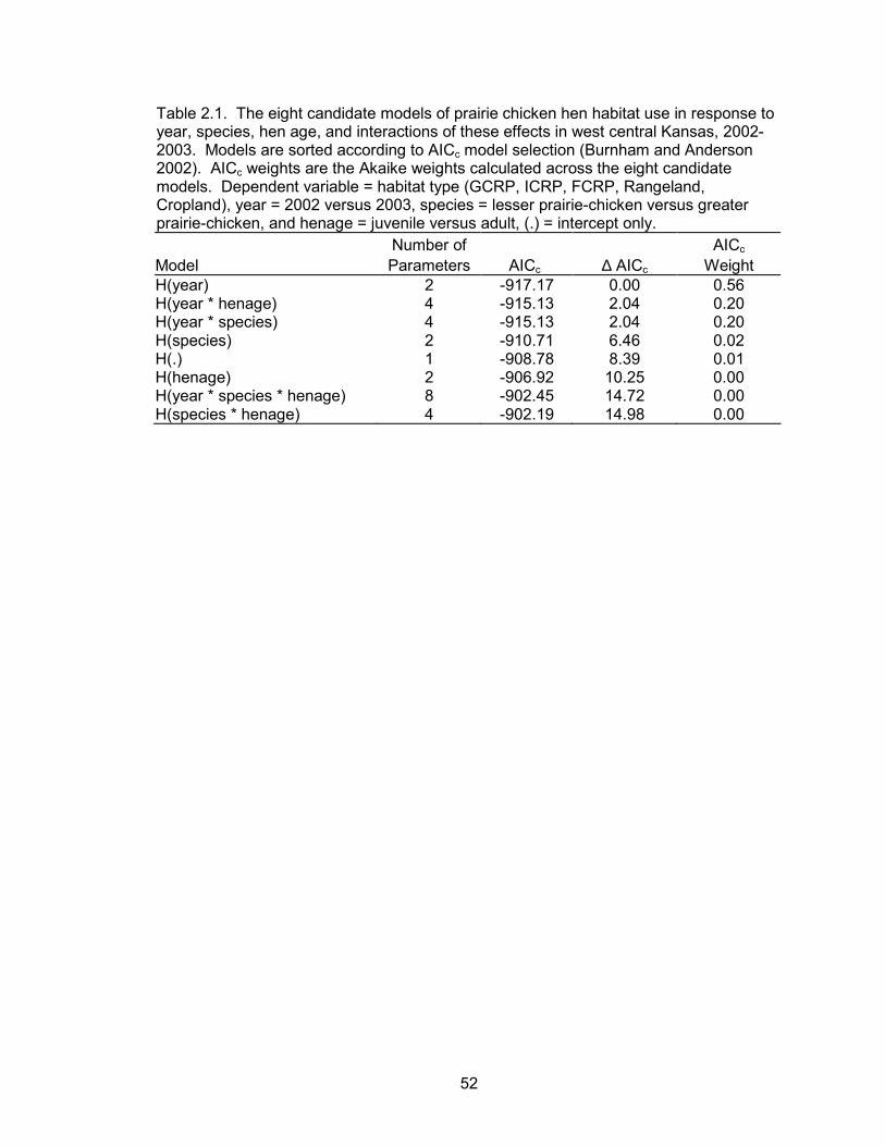
52

Table 2.1. The eight candidate models of prairie chicken hen habitat use in response to year, species, hen age, and interactions of these effects in west central Kansas, 2002-2003. Models are sorted according to AICc model selection (Burnham and Anderson 2002). AICc weights are the Akaike weights calculated across the eight candidate models. Dependent variable = habitat type (GCRP, ICRP, FCRP, Rangeland, Cropland), year = 2002 versus 2003, species = lesser prairie-chicken versus greater prairie-chicken, and henage = juvenile versus adult, (.) = intercept only. Number of AICc Model Parameters AICc ∆ AICc Weight H(year) 2 -917.17 0.00 0.56 H(year * henage) 4 -915.13 2.04 0.20 H(year * species) 4 -915.13 2.04 0.20 H(species) 2 -910.71 6.46 0.02 H(.) 1 -908.78 8.39 0.01 H(henage) 2 -906.92 10.25 0.00 H(year * species * henage) 8 -902.45 14.72 0.00 H(species * henage) 4 -902.19 14.98 0.00

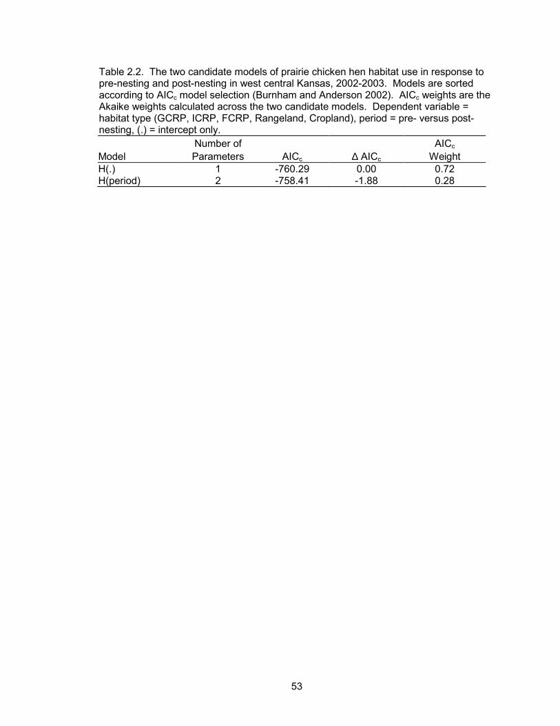
53

Table 2.2. The two candidate models of prairie chicken hen habitat use in response to pre-nesting and post-nesting in west central Kansas, 2002-2003. Models are sorted according to AICc model selection (Burnham and Anderson 2002). AICc weights are the Akaike weights calculated across the two candidate models. Dependent variable = habitat type (GCRP, ICRP, FCRP, Rangeland, Cropland), period = pre- versus post-nesting, (.) = intercept only. Number of AICc Model Parameters AICc ∆ AICc Weight H(.) 1 -760.29 0.00 0.72 H(period) 2 -758.41 -1.88 0.28

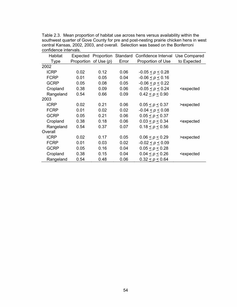
54

Table 2.3. Mean proportion of habitat use across hens versus availability within the southwest quarter of Gove County for pre and post-nesting prairie chicken hens in west central Kansas, 2002, 2003, and overall. Selection was based on the Bonferroni confidence intervals.

Habitat Expected Proportion Standard Confidence Interval Use Compared Type Proportion of Use (p) Error Proportion of Use to Expected

2002 ICRP 0.02 0.12 0.06 -0.05 < p < 0.28 FCRP 0.01 0.05 0.04 -0.06 < p < 0.16 GCRP 0.05 0.08 0.05 -0.06 < p < 0.22 Cropland 0.38 0.09 0.06 -0.05 < p < 0.24 <expected Rangeland 0.54 0.66 0.09 0.42 < p < 0.90 2003 ICRP 0.02 0.21 0.06 0.05 < p < 0.37 >expected FCRP 0.01 0.02 0.02 -0.04 < p < 0.08 GCRP 0.05 0.21 0.06 0.05 < p < 0.37 Cropland 0.38 0.18 0.06 0.03 < p < 0.34 <expected Rangeland 0.54 0.37 0.07 0.18 < p < 0.56 Overall ICRP 0.02 0.17 0.05 0.06 < p < 0.29 >expected FCRP 0.01 0.03 0.02 -0.02 < p < 0.09 GCRP 0.05 0.16 0.04 0.05 < p < 0.28 Cropland 0.38 0.15 0.04 0.04 < p < 0.26 <expected Rangeland 0.54 0.48 0.06 0.32 < p < 0.64

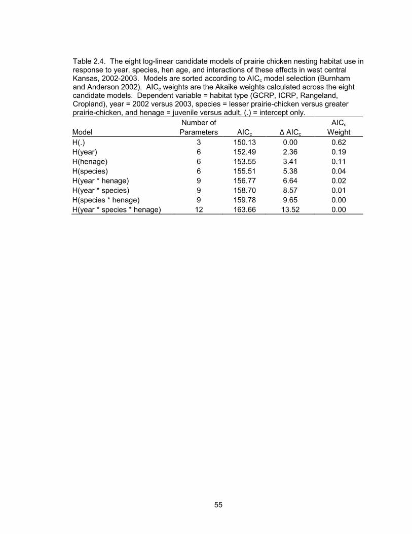
55

Table 2.4. The eight log-linear candidate models of prairie chicken nesting habitat use in response to year, species, hen age, and interactions of these effects in west central Kansas, 2002-2003. Models are sorted according to AICc model selection (Burnham and Anderson 2002). AICc weights are the Akaike weights calculated across the eight candidate models. Dependent variable = habitat type (GCRP, ICRP, Rangeland, Cropland), year = 2002 versus 2003, species = lesser prairie-chicken versus greater prairie-chicken, and henage = juvenile versus adult, (.) = intercept only. Number of AICc Model Parameters AICc ∆ AICc Weight H(.) 3 150.13 0.00 0.62 H(year) 6 152.49 2.36 0.19 H(henage) 6 153.55 3.41 0.11 H(species) 6 155.51 5.38 0.04 H(year * henage) 9 156.77 6.64 0.02 H(year * species) 9 158.70 8.57 0.01 H(species * henage) 9 159.78 9.65 0.00 H(year * species * henage) 12 163.66 13.52 0.00

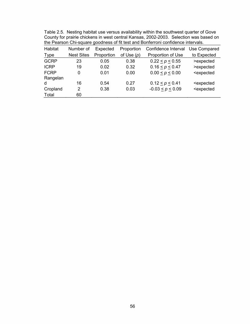
56

Table 2.5. Nesting habitat use versus availability within the southwest quarter of Gove County for prairie chickens in west central Kansas, 2002-2003. Selection was based on the Pearson Chi-square goodness of fit test and Bonferroni confidence intervals. Habitat Number of Expected Proportion Confidence Interval Use ComparedType Nest Sites Proportion of Use (p) Proportion of Use to Expected GCRP 23 0.05 0.38 0.22 < p < 0.55 >expected ICRP 19 0.02 0.32 0.16 < p < 0.47 >expected FCRP 0 0.01 0.00 0.00 < p < 0.00 <expected Rangeland 16 0.54 0.27 0.12 < p < 0.41 <expected Cropland 2 0.38 0.03 -0.03 < p < 0.09 <expected Total 60

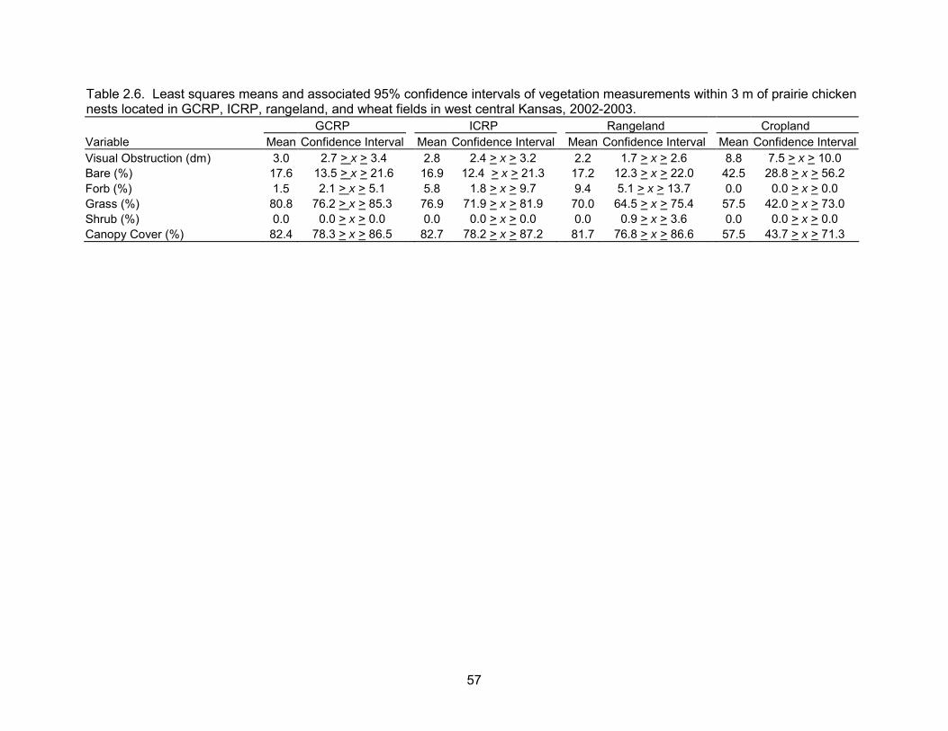
57

Table 2.6. Least squares means and associated 95% confidence intervals of vegetation measurements within 3 m of prairie chicken nests located in GCRP, ICRP, rangeland, and wheat fields in west central Kansas, 2002-2003. GCRP ICRP Rangeland Cropland Variable Mean Confidence Interval Mean Confidence Interval Mean Confidence Interval Mean Confidence IntervalVisual Obstruction (dm) 3.0 2.7 > x > 3.4 2.8 2.4 > x > 3.2 2.2 1.7 > x > 2.6 8.8 7.5 > x > 10.0 Bare (%) 17.6 13.5 > x > 21.6 16.9 12.4 > x > 21.3 17.2 12.3 > x > 22.0 42.5 28.8 > x > 56.2 Forb (%) 1.5 2.1 > x > 5.1 5.8 1.8 > x > 9.7 9.4 5.1 > x > 13.7 0.0 0.0 > x > 0.0 Grass (%) 80.8 76.2 > x > 85.3 76.9 71.9 > x > 81.9 70.0 64.5 > x > 75.4 57.5 42.0 > x > 73.0 Shrub (%) 0.0 0.0 > x > 0.0 0.0 0.0 > x > 0.0 0.0 0.9 > x > 3.6 0.0 0.0 > x > 0.0 Canopy Cover (%) 82.4 78.3 > x > 86.5 82.7 78.2 > x > 87.2 81.7 76.8 > x > 86.6 57.5 43.7 > x > 71.3

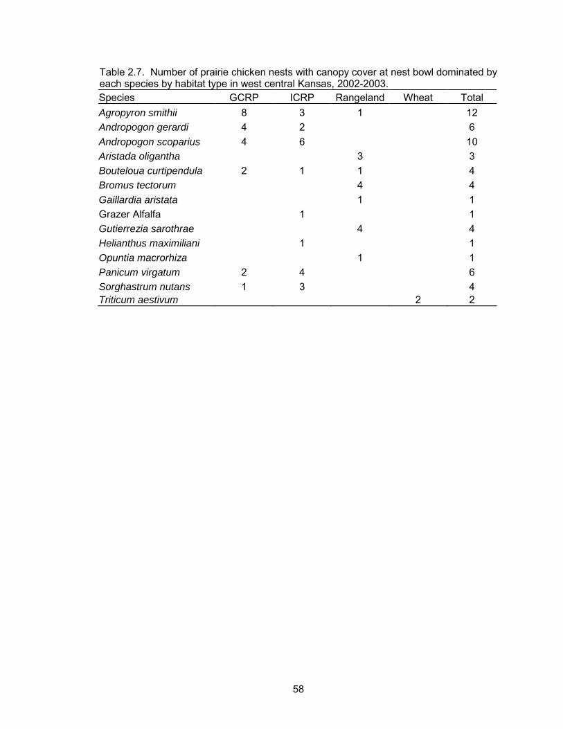
58

Table 2.7. Number of prairie chicken nests with canopy cover at nest bowl dominated by each species by habitat type in west central Kansas, 2002-2003. Species GCRP ICRP Rangeland Wheat Total Agropyron smithii 8 3 1 12 Andropogon gerardi 4 2 6 Andropogon scoparius 4 6 10 Aristada oligantha 3 3 Bouteloua curtipendula 2 1 1 4 Bromus tectorum 4 4 Gaillardia aristata 1 1 Grazer Alfalfa 1 1 Gutierrezia sarothrae 4 4 Helianthus maximiliani 1 1 Opuntia macrorhiza 1 1 Panicum virgatum 2 4 6 Sorghastrum nutans 1 3 4 Triticum aestivum 2 2

59

Table 2.8. The eight candidate models of prairie chicken brood habitat use in response to year, species, hen age, and interactions of these effects in west central Kansas, 2002-2003. Models are sorted according to AICc model selection (Burnham and Anderson 2002). AICc weights are the Akaike weights calculated across the eight candidate models. Dependent variable = habitat type (GCRP, ICRP, Rangeland, Cropland), year = 2002 versus 2003, species = lesser prairie-chicken versus greater prairie-chicken, and henage = juvenile versus adult, (.) = intercept only. Number of AICc Model Parameters AICc ∆ AICc Weight H(.) 1 -295.97 0.00 0.60 H(species) 2 -294.43 1.54 0.28 H(year) 2 -292.4 3.57 0.10 H(henage) 2 -288.36 7.61 0.01 H(species * henage) 4 -277.47 18.50 0.00 H(year * henage) 4 -277.31 18.66 0.00 H(year * species) 4 -277.31 18.66 0.00 H(year * species * henage) 8 -241.62 54.35 0.00

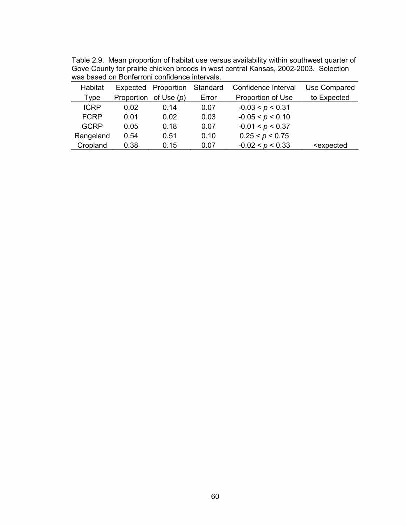
60

Table 2.9. Mean proportion of habitat use versus availability within southwest quarter of Gove County for prairie chicken broods in west central Kansas, 2002-2003. Selection was based on Bonferroni confidence intervals.

Habitat Expected Proportion Standard Confidence Interval Use Compared Type Proportion of Use (p) Error Proportion of Use to Expected ICRP 0.02 0.14 0.07 -0.03 < p < 0.31 FCRP 0.01 0.02 0.03 -0.05 < p < 0.10 GCRP 0.05 0.18 0.07 -0.01 < p < 0.37

Rangeland 0.54 0.51 0.10 0.25 < p < 0.75 Cropland 0.38 0.15 0.07 -0.02 < p < 0.33 <expected

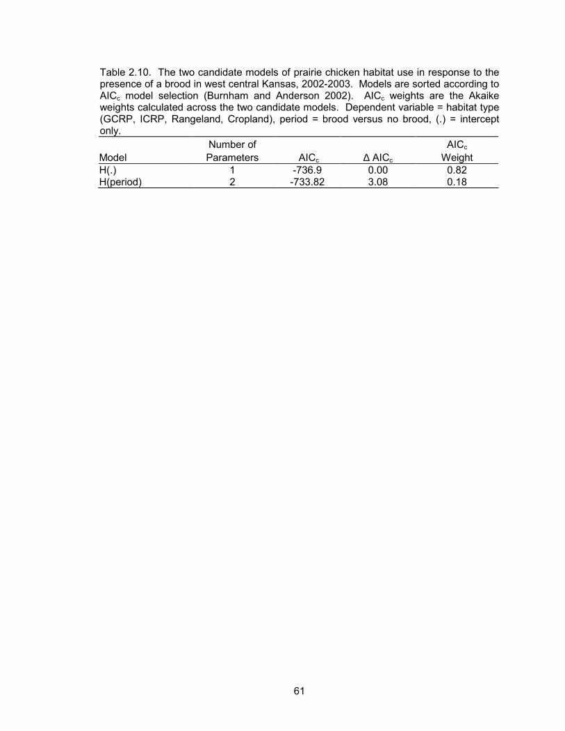
61

Table 2.10. The two candidate models of prairie chicken habitat use in response to the presence of a brood in west central Kansas, 2002-2003. Models are sorted according to AICc model selection (Burnham and Anderson 2002). AICc weights are the Akaike weights calculated across the two candidate models. Dependent variable = habitat type (GCRP, ICRP, Rangeland, Cropland), period = brood versus no brood, (.) = intercept only. Number of AICc Model Parameters AICc ∆ AICc Weight H(.) 1 -736.9 0.00 0.82 H(period) 2 -733.82 3.08 0.18

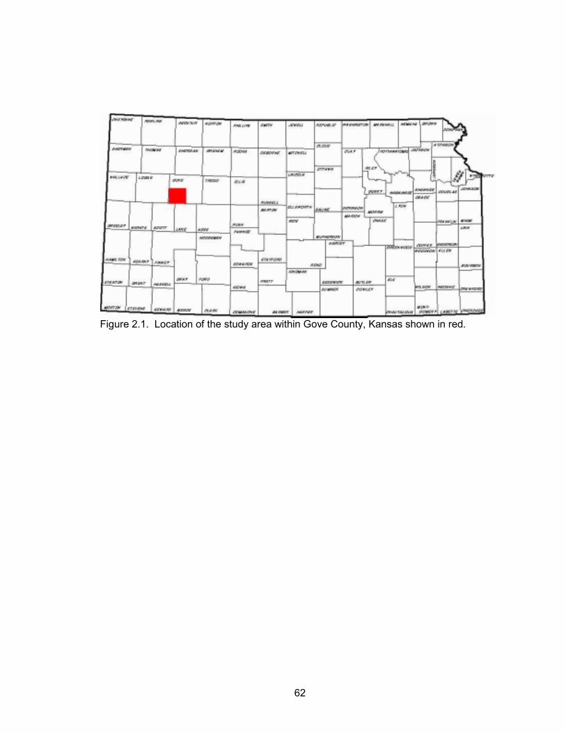
62

Figure 2.1. Location of the study area within Gove County, Kansas shown in red.

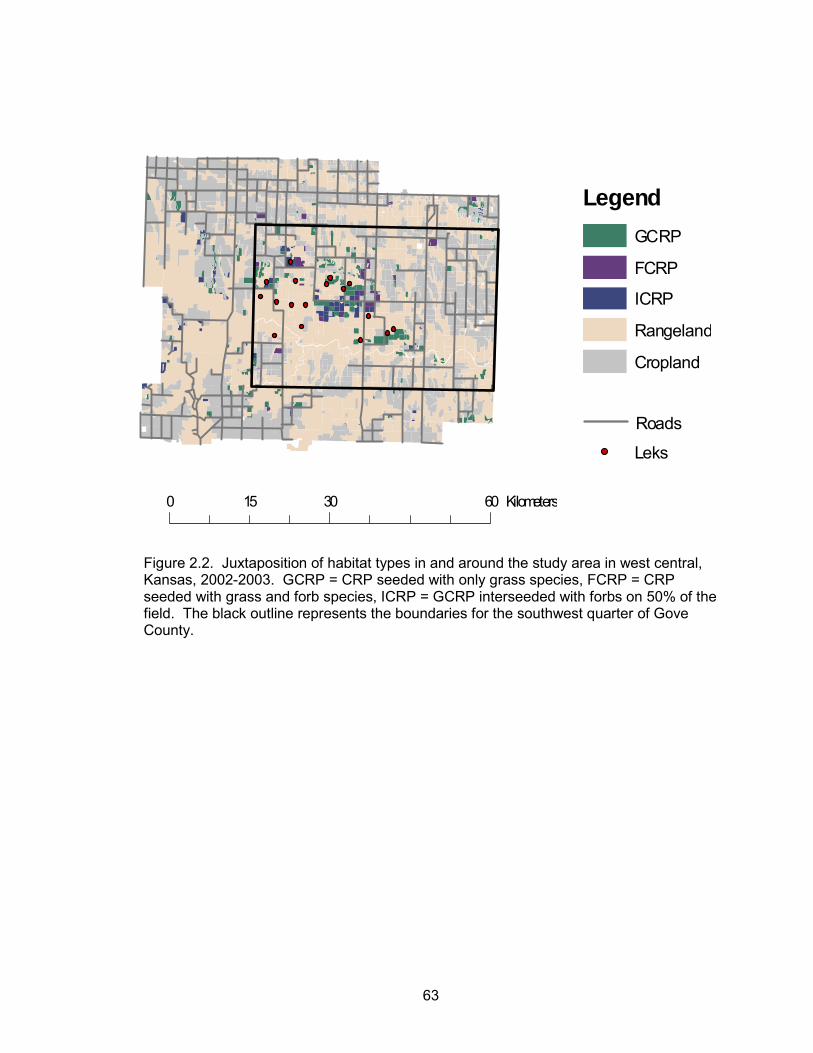
63

Figure 2.2. Juxtaposition of habitat types in and around the study area in west central, Kansas, 2002-2003. GCRP = CRP seeded with only grass species, FCRP = CRP seeded with grass and forb species, ICRP = GCRP interseeded with forbs on 50% of the field. The black outline represents the boundaries for the southwest quarter of Gove County.

0 30 6015 Kilometers

LegendGCRP

FCRP

ICRP

Rangeland

Cropland

Roads

Leks

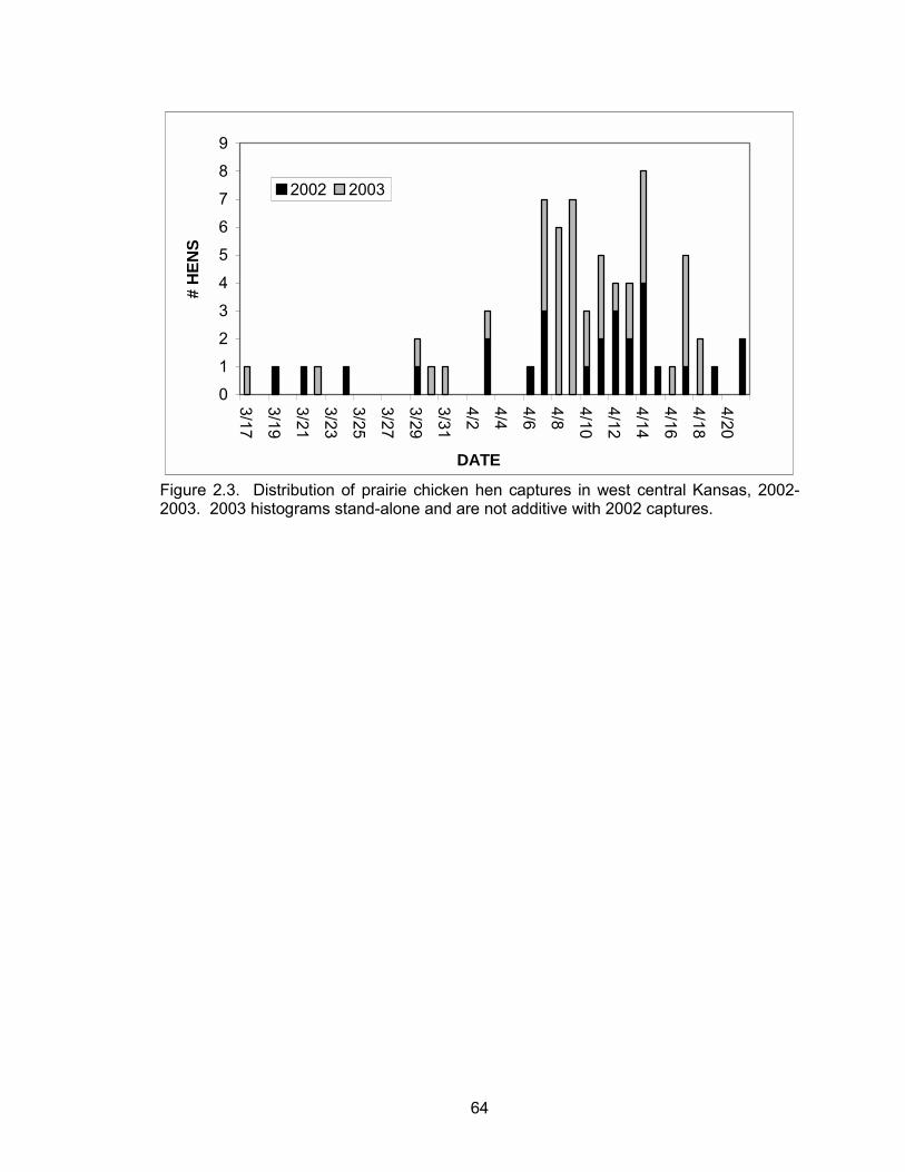
64

0

1

2

3

4

5

6

7

8

9

3/17

3/19

3/21

3/23

3/25

3/27

3/29

3/31

4/2

4/4

4/6

4/8

4/10

4/12

4/14

4/16

4/18

4/20

DATE

# H

ENS

2002 2003

Figure 2.3. Distribution of prairie chicken hen captures in west central Kansas, 2002-2003. 2003 histograms stand-alone and are not additive with 2002 captures.

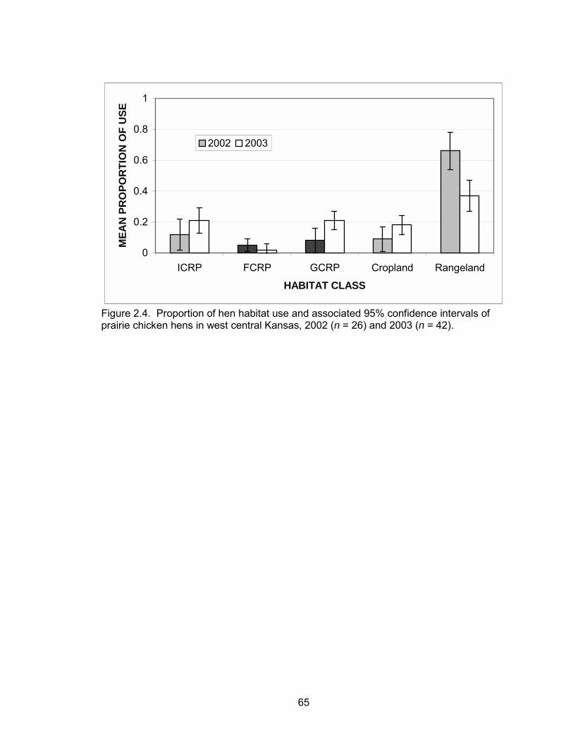
65

0

0.2

0.4

0.6

0.8

1

ICRP FCRP GCRP Cropland Rangeland

HABITAT CLASS

MEA

N P

RO

POR

TIO

N O

F U

SE

2002 2003

Figure 2.4. Proportion of hen habitat use and associated 95% confidence intervals of prairie chicken hens in west central Kansas, 2002 (n = 26) and 2003 (n = 42).

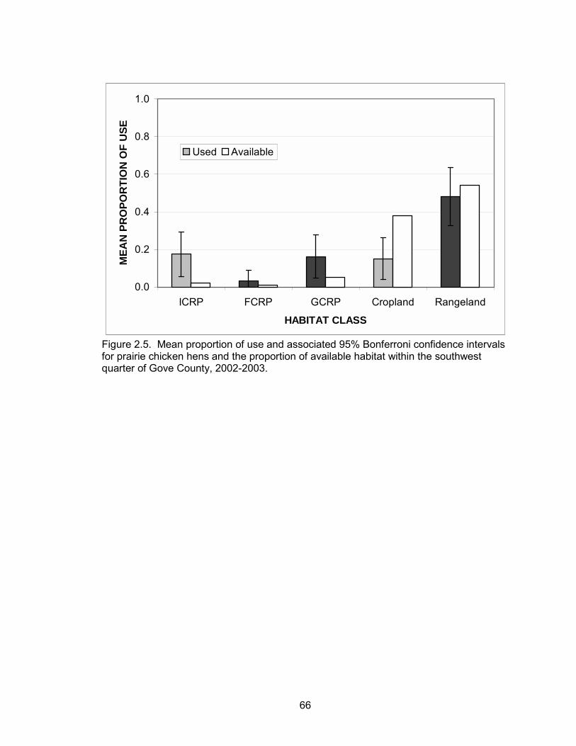
66

0.0

0.2

0.4

0.6

0.8

1.0


HABITAT CLASS

MEA

N P

RO

POR

TIO

N O

F U

SE

Used Available

Figure 2.5. Mean proportion of use and associated 95% Bonferroni confidence intervals for prairie chicken hens and the proportion of available habitat within the southwest quarter of Gove County, 2002-2003.

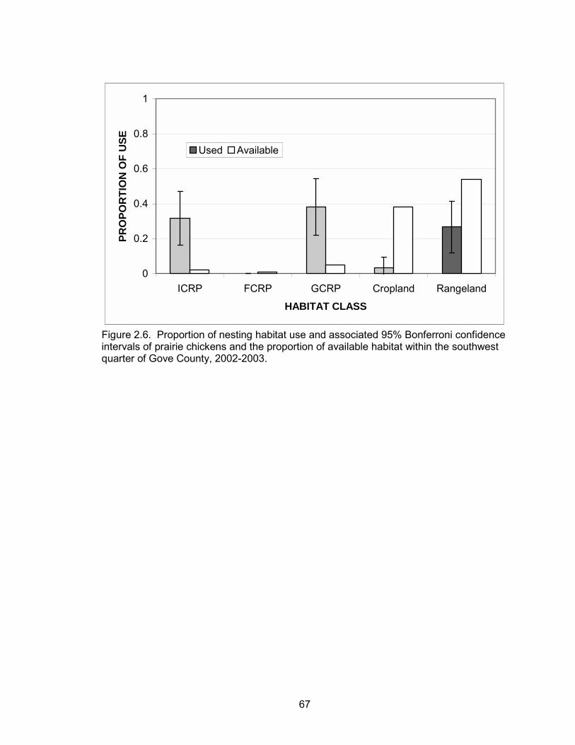
67

0

0.2

0.4

0.6

0.8

1


HABITAT CLASS

PRO

POR

TIO

N O

F U

SE

Used Available

Figure 2.6. Proportion of nesting habitat use and associated 95% Bonferroni confidence intervals of prairie chickens and the proportion of available habitat within the southwest quarter of Gove County, 2002-2003.

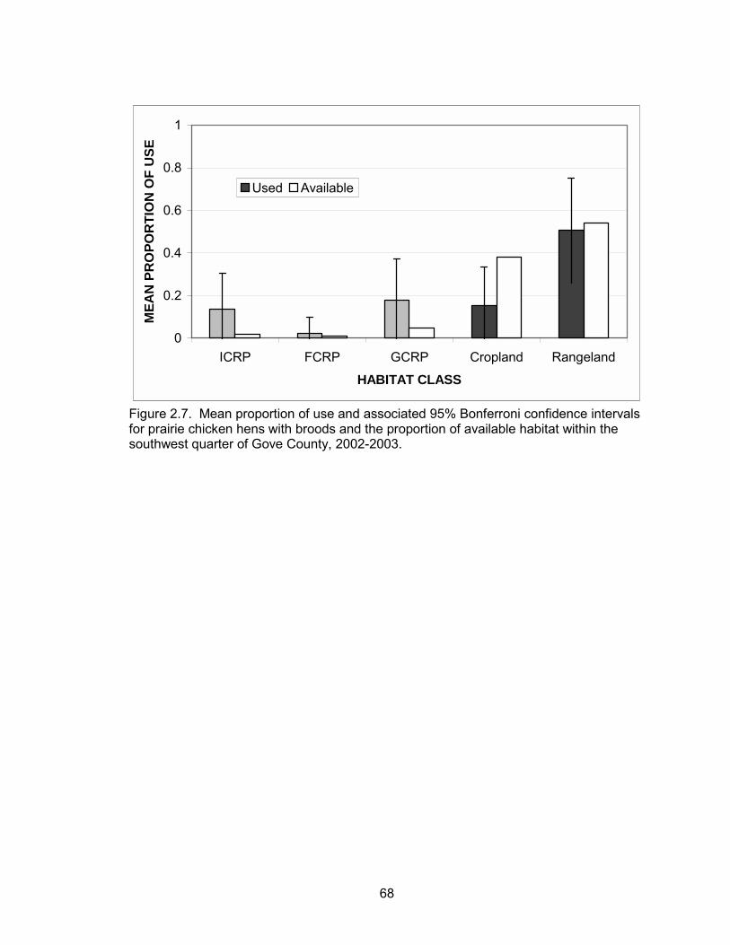
68

0

0.2

0.4

0.6

0.8

1


HABITAT CLASS

MEA

N P

RO

POR

TIO

N O

F U

SE

Used Available

Figure 2.7. Mean proportion of use and associated 95% Bonferroni confidence intervals for prairie chicken hens with broods and the proportion of available habitat within the southwest quarter of Gove County, 2002-2003.

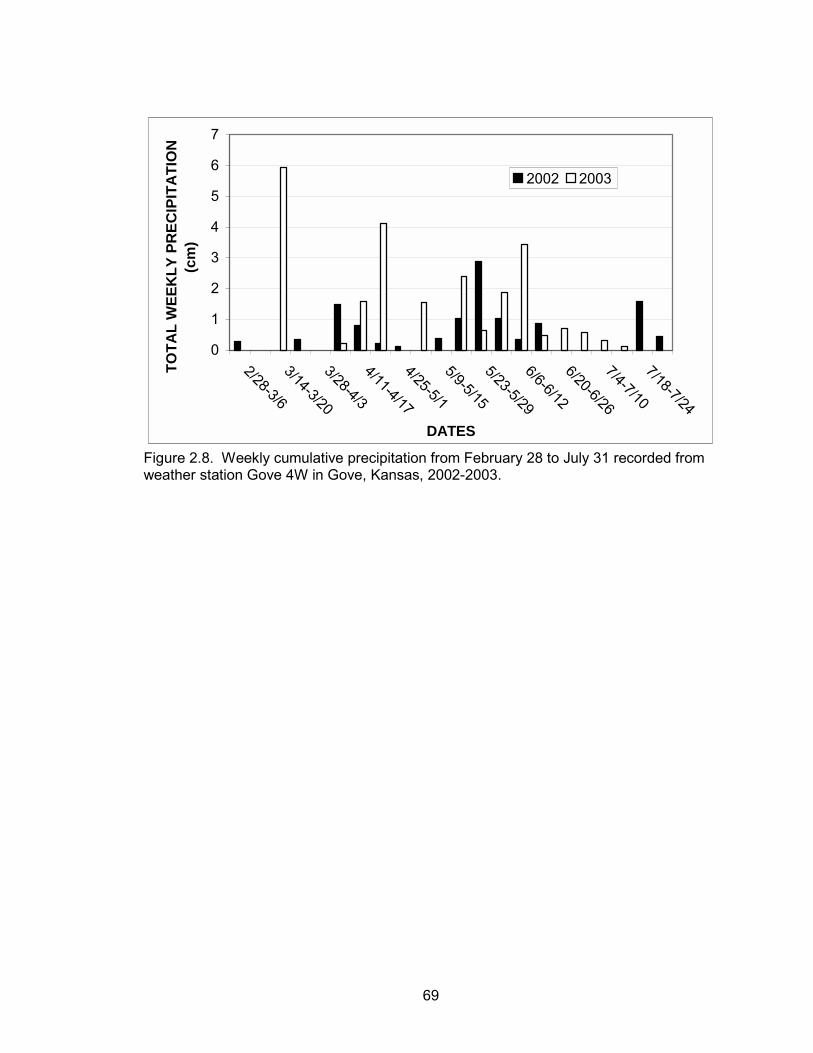
69

0

1

2

3

4

5

6

7

2/28-3/6

3/14-3/20

3/28-4/3

4/11-4/17

4/25-5/1

5/9-5/15

5/23-5/29

6/6-6/12

6/20-6/26

7/4-7/10

7/18-7/24

DATES

TOTA

L W

EEK

LY P

REC

IPIT

ATI

ON

(c

m)

2002 2003

Figure 2.8. Weekly cumulative precipitation from February 28 to July 31 recorded from weather station Gove 4W in Gove, Kansas, 2002-2003.

70

CHAPTER 3: SURVIVAL OF PRAIRIE CHICKEN HENS, NESTS, AND BROODS

INTRODUCTION

The lesser prairie-chicken (Tympanuchus pallidicinctus) has the smallest and

most restricted range of any North American grouse species (Giesen 1998). As a result

of a 92% reduction in range, lesser prairie-chicken populations have declined by

approximately 97% since the late 1800s (Crawford 1980, Taylor and Guthery 1980).

Declines have been attributed to conversion of native rangelands to croplands and

pastures consisting of introduced species and excessive livestock grazing on rangelands

(Crawford 1980, Taylor and Guthery 1980, Bidwell 2002). Excessive livestock grazing

appears detrimental when reduction in height and density of vegetation results in

decreased nest and brood success (Candelaria 1979, Davis et al. 1979, Sell 1979,

Ahlborn 1980, Huakos and Smith 1989, Giesen 1994). Tree invasions and plantings,

fences, phone lines, and gas, oil and wind developments threaten populations as well

(Bidwell et al. 2002). Recurrent droughts of the 1930s, 1950s, and 1990s have

compounded the effects of these anthropogenic activities (Giesen 1998). In response to

range-wide declines, the lesser prairie-chicken was petitioned for listing as threatened

under the Endangered Species Act of 1973. The U.S. Fish and Wildlife Service

(USFWS) concluded that the petition was warranted, but precluded because of higher

priority species (U.S. Department of the Interior 2002).

In Kansas, recent lesser prairie-chicken population declines occurred between

the mid 1970s and the mid 1990s. Counts of leks and individual birds indicate that

populations within Kansas have experienced significant declines since 1964 (Jensen et

al. 2000). According to Applegate and Riley (1998), lesser prairie-chicken populations

71

have declined by between 15 and 20% since the early 1990�s. These declines have

been attributed to habitat deterioration, an increase in center-pivot crop fields, and to the

drought years of 1990 and 1991 (Applegate and Riley 1998, Jamison 2000, Jensen et al.

2000). Conversion to center pivot crop fields was reduced in the early 1980�s, but

population surveys reported a continued decline (Jamison 2000).

Nest survival and survival of juvenile prairie grouse have been identified as the

two most critical demographic parameters associated with prairie grouse population size

(Peterson and Silvy 1996, Wisdom and Mills 1997). Vegetation height and density,

percent grass cover, and the abundance of bluestem grasses (Andropogon spp.) have

been associated with apparent nest success (percent of nests hatching > 1 chick) in a

number of studies (Riley 1978, Wisdom 1980, Riley et al. 1992, Pitman 2003).

Additionally, the negative effects of moderate to heavy grazing (Riley 1978, Davis et al.

1979, Wisdom 1980, Huakos and Smith 1989) and drought conditions (Giesen 1998) on

nest success have been documented. Estimates of nest success averaged 28% with a

range of 0 to 67% for 10 studies in four states (Giesen 1998). Apparent nest success

in southwestern Kansas on two sand sagebrush (Artemesia filifolia) prairie fragments

was 26% over a 6-year period (Pitman 2003).

Invertebrate biomass, brood movements, and vegetation structure are thought to

be the primary factors associated with chick survival (Bergerud and Gratson 1988).

Invertebrate abundance was positively associated with juvenile grouse survival in

several studies (Erikstad 1985, Park et al. 2001). Erikstad (1985) also noted a negative

relationship between chick survival and movements. Erikstad (1985) concluded that

chicks increased movements when invertebrates were limited. A quadratic relationship

between sagebrush density and lesser prairie-chicken chick survival was found in

southwestern Kansas (Pitman 2003).

Chick survival estimates, calculated by dividing average brood size by average

72

clutch size, have ranged from 0.27 to 0.65 in three states (Davison 1940, Schwilling

1955, Copelin 1963, Merchant 1982). These studies most likely overestimated survival

due to the failure to account for complete brood losses (Jamison 2000). In Kansas,

Pitman (2003) calculated chick survival using the Mayfield estimator (Mayfield 1975).

Chick survival was 0.48, 0.37, and 0.18 for the pre-fledge, the post-fledge, and the entire

60-day period, respectively.

In contrast to range-wide and statewide declines, lesser prairie-chicken

populations have recently expanded northward and westward in Kansas. According to

the Kansas Department of Wildlife and Parks (KWP), the currently reoccupied area was

part of their historic range and included populations of lesser prairie-chickens prior to

1963. After 1963, their range continued to decline until just recently (R. D. Rodgers,

Kansas Department of Wildlife and Parks, personal communication). In addition to the

expansion of lesser prairie-chickens, greater prairie-chickens (Tympanuchus cupido)

currently inhabit the area. The increase of prairie chickens within west central Kansas

has been attributed to the influence of the Pheasant Initiative Priority Area designation

on Conservation Reserve Program (CRP) management. In particular, the expansion

has been attributed to an increase in reproductive success resulting from forb

interseeding on grass CRP fields.

In 1986, CRP was initiated in Gove County, Kansas by the 1985 Farm Bill. It is

currently administered by the Natural Resource Conservation Service (NRCS). This

program requires the seeding of highly erodible agricultural fields with native grass

species. Prior to 1997, CRP fields consisted of only grass species (GCRP). In 1997,

interseeding of CRP fields, as a management strategy to improve wildlife habitat, was

implemented (ICRP). Fifty percent of each designated grass CRP field within the study

area was interseeded with forbs by the NRCS or the KWP. In 1998, the use of forbs

within the grass seed mixtures was initiated (FCRP).

73

The objective of this study was to evaluate the effect of habitat use and other

sources of variation on survival of hens, nests, and broods. To evaluate this objective, I

hypothesized that survival of hens would be greatest in ICRP due to the cover and food

source it provides. I hypothesized that nest survival would be greatest in ICRP and

GCRP due to the density and height of vegetation within these habitat types. I

hypothesized that brood survival would be greatest in ICRP and FCRP due to the

vegetative structure and the availability of forbs within these habitat types.

METHODS

Locating and Monitoring Hens

Refer to Chapter 2 for study area description. Research protocol was approved

by the Colorado State University Animal Care and Use Committee (Protocol approval

number: 01-283A-02). Female prairie chickens were captured on leks in the spring

using walk-in traps from March 14 - April 21, 2002 and 2003. All captured birds were

classified as yearlings (~10 months of age) or adults by examining the primary feathers

(Copelin 1963, D. Wolfe, Sutton Avian Research Center, personal communication).

Greater prairie-chickens were also distinguished from lesser prairie-chickens. Species

identification was confirmed using a DNA blood sample analysis from all hens in 2002.

Prairie chicken was used to collectively refer to both species. Body mass of all captured

hens was measured using a Pesola® spring scale. Each captured hen was fitted with

battery-powered radio transmitters weighing approximately 11 g (R1-2B Holohil with

mortality sensors) and released immediately.

Birds equipped with transmitters were relocated daily using an ATS 4-element

antenna mounted on a hand-held mast and an ATS R2000 scanning receiver or an ATS

FM100 receiver from the day of capture until July 31. Hens with broods were relocated

daily from hatch to 60 days post-hatch. All radio-collared individuals were located by

74

homing until the type of habitat occupied was determined. Missing hens were radio-

located using extensive ground searches or aerial telemetry from a Cessna 150 aircraft.

After a bird remained in the same location for 3 to 4 successive days, it was

considered incubating. At this time, nesting hens were flushed off their nest and UTM

coordinates and clutch size were recorded. Nests were monitored on a daily basis by

taking 2-3 bearings from set locations to determine if the hen was still on her nest. The

nest was revisited when the nest failed or successfully hatched (produced > 1 chick).

The number of eggs that successfully hatched, infertile eggs and depredated eggs were

recorded. If the nest was depredated, the area around the nest was searched for tracks,

scat, and eggshell fragments to determine the potential depredator�s identity (Sargeant

et al. 1998).

Vegetation Sampling

Percent canopy cover of shrubs, forbs, grasses, and bare ground was estimated

using eight 20 x 50 cm frames (Daubenmire 1959) at the nest bowl and at 3 m NW, SW,

SE, and NE of the nest bowl. Eight visual obstruction readings (VOR) were estimated

using a Robel pole at the nest bowl and at 3 m SW, NW, NE, and SE of the nest bowl.

Readings were taken from a height of 1.0 m and a distance of 4.0 m at mid-day. The

lowest decimeter or half-decimeter mark visible was recorded (Robel et al. 1970). In

addition to the canopy cover and visual obstruction measurements, the vegetative

species with the highest percentage of canopy cover above the nest bowl was recorded.

Brood site locations were characterized by ocular estimates taken at brood

locations daily. Percent canopy cover of forbs, grasses, shrubs, and bareground, total

canopy cover, and vegetation height were estimated within 50 m of the brood sites

without flushing the brood. A numerical value from 0 to 10 was assigned for forbs,

grasses, shrubs and bareground. The following index was used when evaluating

composition within a habitat:

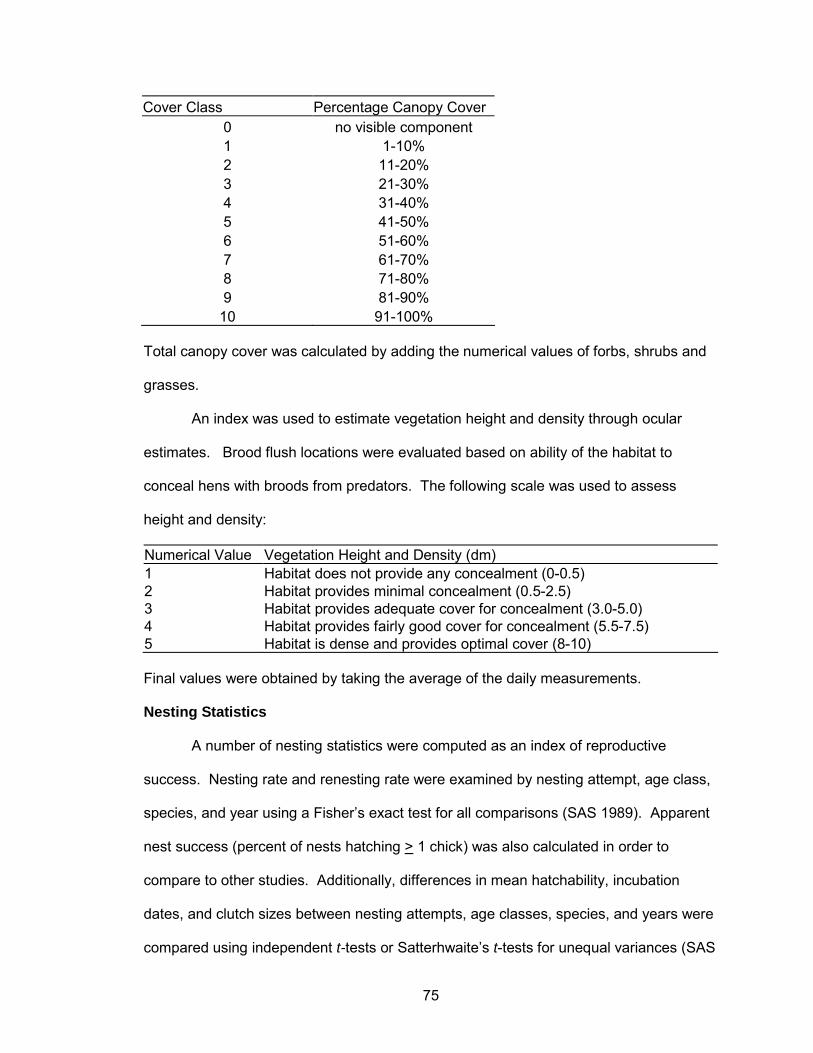
75

Cover Class Percentage Canopy Cover 0 no visible component 1 1-10% 2 11-20% 3 21-30% 4 31-40% 5 41-50% 6 51-60% 7 61-70% 8 71-80% 9 81-90%

10 91-100% Total canopy cover was calculated by adding the numerical values of forbs, shrubs and

grasses.

An index was used to estimate vegetation height and density through ocular

estimates. Brood flush locations were evaluated based on ability of the habitat to

conceal hens with broods from predators. The following scale was used to assess

height and density:

Numerical Value Vegetation Height and Density (dm) 1 Habitat does not provide any concealment (0-0.5) 2 Habitat provides minimal concealment (0.5-2.5) 3 Habitat provides adequate cover for concealment (3.0-5.0) 4 Habitat provides fairly good cover for concealment (5.5-7.5) 5 Habitat is dense and provides optimal cover (8-10) Final values were obtained by taking the average of the daily measurements.

Nesting Statistics

A number of nesting statistics were computed as an index of reproductive

success. Nesting rate and renesting rate were examined by nesting attempt, age class,

species, and year using a Fisher�s exact test for all comparisons (SAS 1989). Apparent

nest success (percent of nests hatching > 1 chick) was also calculated in order to

compare to other studies. Additionally, differences in mean hatchability, incubation

dates, and clutch sizes between nesting attempts, age classes, species, and years were

compared using independent t-tests or Satterhwaite�s t-tests for unequal variances (SAS

76

1989). Hatchability was defined as the percent of eggs hatching within successful nests.

Brood Statistics

Systematic flushes were used to determine if a hen had a brood. Radio-collared

females that nested successfully were flushed 14 days post-hatch to count the number

of chicks. Subsequent flushes were conducted at 37 and 60 days post-hatch. Counts

were corrected when subsequent flushes revealed an incomplete count during the

previous flush. The number of chicks per brood at hatch, 14 days and 60 days and

mean recruitment rate to 60 days were examined as an indicator of breeding success.

Apparent brood survival (percent of broods > 1 chick) at 14 and 60 days was also

calculated to compare to other studies.

Data collected from brood flushes were also used to calculate pre-fledge (hatch

to 14 days) and post-fledge (15 to 60 days) daily survival rates ( RSD � ). The number of

chicks believed to have hatched out of a clutch was used as the initial brood size for pre-

fledge estimates. Chicks surviving until 14 days post-hatch were used as the initial

brood size for post-fledge estimates. Daily survival rates were calculated across broods

( RSD � ) for each period using the following equation:

days

Ct

Ct

NNRSD

/#11�

= +

where NC is the number of chicks at time t or time t+1. Overall survival rates for each

period were calculated by raising daily survival rates to the power of 14 and 46 for pre-

and post-fledge broods, respectively. Survival from hatch to 60 days post-hatch was

calculated by multiplying chick survival from the two periods.

Survival Analyses

Program MARK was used to model survival probabilities of hens, nests, and

broods as a function of time-specific and individual covariates (White and Burnham

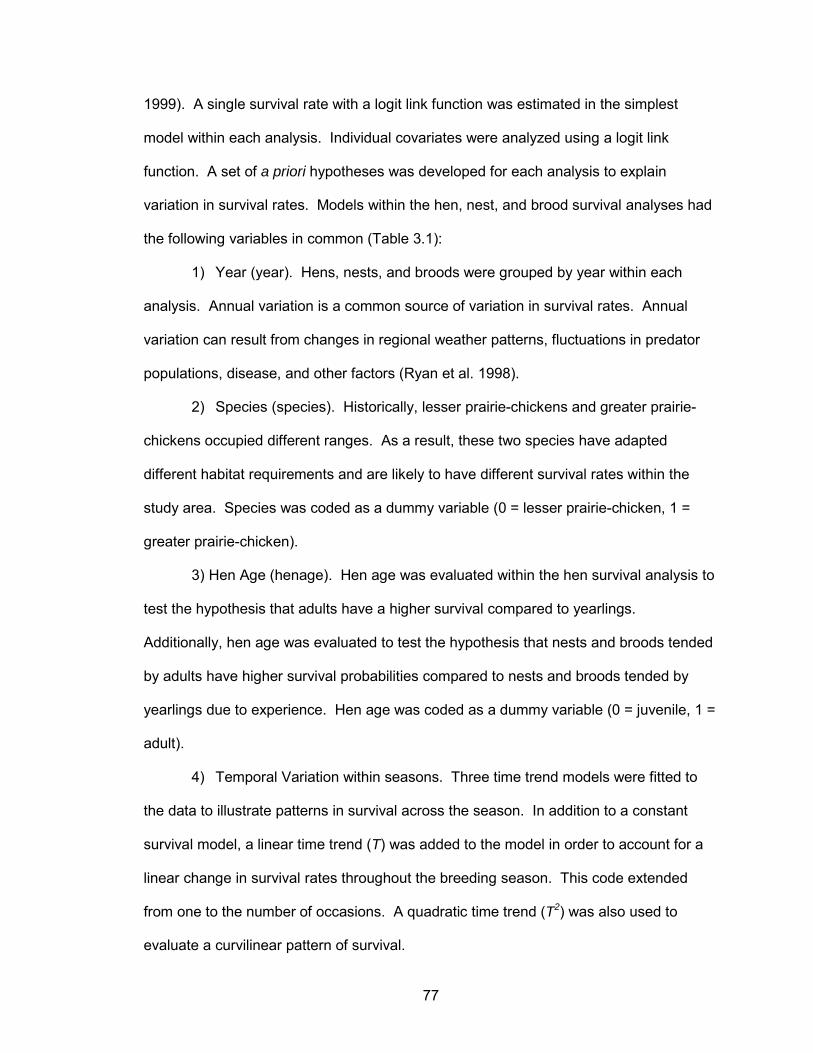
77

1999). A single survival rate with a logit link function was estimated in the simplest

model within each analysis. Individual covariates were analyzed using a logit link

function. A set of a priori hypotheses was developed for each analysis to explain

variation in survival rates. Models within the hen, nest, and brood survival analyses had

the following variables in common (Table 3.1):

1) Year (year). Hens, nests, and broods were grouped by year within each

analysis. Annual variation is a common source of variation in survival rates. Annual

variation can result from changes in regional weather patterns, fluctuations in predator

populations, disease, and other factors (Ryan et al. 1998).

2) Species (species). Historically, lesser prairie-chickens and greater prairie-

chickens occupied different ranges. As a result, these two species have adapted

different habitat requirements and are likely to have different survival rates within the

study area. Species was coded as a dummy variable (0 = lesser prairie-chicken, 1 =

greater prairie-chicken).

3) Hen Age (henage). Hen age was evaluated within the hen survival analysis to

test the hypothesis that adults have a higher survival compared to yearlings.

Additionally, hen age was evaluated to test the hypothesis that nests and broods tended

by adults have higher survival probabilities compared to nests and broods tended by

yearlings due to experience. Hen age was coded as a dummy variable (0 = juvenile, 1 =

adult).

4) Temporal Variation within seasons. Three time trend models were fitted to

the data to illustrate patterns in survival across the season. In addition to a constant

survival model, a linear time trend (T) was added to the model in order to account for a

linear change in survival rates throughout the breeding season. This code extended

from one to the number of occasions. A quadratic time trend (T2) was also used to

evaluate a curvilinear pattern of survival.

78

In addition to these variables, survival analyses included sources of variation

specific to hens, nests, and broods (Table 3.1). All weather data were obtained from the

Gove 4W weather station located in Gove, Kansas approximately 18.5 km northeast

from the center of the study area.

Each set of candidate models was ranked based on small sample Akaike�s

Information Criteria (AICc; Akaike 1973, Burnham and Anderson 2002). Variable

weights were computed to assess the relative importance of variables within each

analysis (Burnham and Anderson 2002). Variable weights were calculated by summing

the Akaike weights of models that included the variable of interest. Beta estimates were

also reported to demonstrate the direction of associations between survival rates and

variables. For categorical variables, beta estimates represent differences between the

reference variable and subsequent variables within the category of interest. In addition

to evaluating the effects of different sources of variation on survival, the best model from

each analysis was used to estimate model-conditional survival estimates.

Hens.--The known fate data type in Program MARK was used to model weekly

survival probabilities of hens because they were radio-collared and tracked daily (White

and Burnham 1999). Hens that were suspected of emigrating from the study area were

censored if they were not located during aerial searches. Only hens that survived more

than one week following capture were included within the analysis, because mortalities

occurring shortly after capture may have been a result of capture related stress. Twenty

encounter occasions were used to estimate weekly survival probabilities from March 14

to July 31. Capture histories for each hen were coded with a live dead sequence

(LDLDLD). The following additional variables were included within the candidate models

(Table 3.1):

1) Dominant habitat type (habitat). Dominant habitat type for each hen was

designated based on number of locations within each habitat type. The dominant habitat

79

for each hen was the habitat type with the most locations. I hypothesized that hens

using ICRP and GCRP would have higher survival compared to hens using rangeland,

cropland, or FCRP due to higher residual grass cover and canopy cover. ICRP also

provides areas with high forb canopy cover. Dominant habitat type was coded using 4

dummy variables with rangeland as the reference habitat (0 0 0 0).

2) Heating degree-days (hdd). Number of days per week exceeding 35 C was

used as a heat stress index (Flanders 2002). I hypothesized that hen survival would

decrease with an increase in the number of heating degree-days. High temperatures

may also indirectly increase survival over the long term by impacting invertebrate

hatches.

3) Total weekly precipitation (cm) (precip). Mammalian predators may be able

to better search out hens following precipitation events due to an increase in hen odor

and reduced movement. Therefore, I surmised that hen survival would be negatively

correlated with precipitation events. There is also a potential positive relationship

between precipitation and survival due to the response of vegetation to precipitation

events.

Candidate models were run with all one-, two-, and three-way additive

combinations of these variables. Weekly survival probabilities were calculated using

maximum likelihood estimates. The combined likelihood (L) for weekly survival (Si) from

day i to day i+1 for a hen is:

( ) ( ) ( ) yk

yk

k

kiiii SSSkSL −

−

=

−

= ∏ 1

1

22

2

1

1|

where k1 is the day the hen was captured, k2 is the last day the hen was known to be

alive and y is the fate of the hen (0 = survived, 1 = died). The likelihood for a sample of

birds is the product of these likelihoods (Burnham and Anderson 2002).

Nests.--The known fate data type available in program MARK was used to

80

evaluate daily nest survival probabilities. Capture histories for each nest were coded

with a live dead sequence (LDLDLD) (White and Burnham 1999). The following

additional sources of variation were included (Table 3.1):

1) Nest habitat (habitat). I hypothesized that ICRP and GCRP would have higher

nest survival compared to rangeland due to higher residual grass cover and greater

canopy cover it provides (Jones 1963, Sell 1979, Wisdom 1980, Huakos and Smith

1989, Riley et al. 1992, Giesen 1994). CRP also has a higher density of bluestem

grasses, a preferred nest site species (Wilson 1982, Huakos and Smith 1989). Habitat

type was coded using 3 dummy variables with rangeland as the reference habitat (0 0

0). FCRP was not included because there were no known nests in this habitat type.

2) Nest attempt (attempt). I hypothesized that primary nest attempts would be

more successful than secondary nest attempts because of greater clutch sizes and

better hen condition (Thogmartin and Johnson 1999). Energy lost during egg-laying and

incubation is substantial (Bergerud and Gratson 1988). In addition, nests earlier in the

season experience more favorable weather conditions. Nest attempt was coded as a

dummy variable (0 = primary, 1 = secondary).

3) Nest age (nestage). Nest survival was expected to decrease throughout the

incubation period due to an increase in nest odor and scent trails made by the nesting

hen during feeding. Nests were monitored throughout the nesting season to reduce

potential confounding with temporal variation. Nest age was modeled as a single

parameter and was coded as the negative of the incubation onset Julian day to indicate

when incubation was initiated.

4) Maximum daily temperature (C) (temp). Lower lesser prairie-chicken nest

survival during drought years has been attributed to higher maximum temperatures

(Wilson 1982); therefore, I hypothesized that nest survival would decrease with higher

maximum daily temperatures.

81

5) Daily precipitation (cm) (precip). There are both direct and indirect effects that

may result from daily precipitation events. High rainfall during incubation may increase

humidity, thus increasing the effectiveness of mammalian predators at locating hens on

nests (Palmer et al. 1993, Roberts et al. 1995). One of the primary nest predators, the

bull snake (Pituophis catenifer sayi), shows an increase in activity following precipitation

events (Gibbons and Semlitsch 1987). Research on sage grouse (Centrocercus

urophasianus) in Montana has also demonstrated that heavy precipitation during egg-

laying can reduce productivity (Wallestad and Watts 1972, Eustace 2002). Therefore, I

surmised that nest survival would be negatively correlated with precipitation events.

6) Visual Obstruction Reading (dm) (vor). Studies have found that the height

and density of vegetation may increase nest survival by providing concealment and

protection from extreme temperatures, high winds, low relative humidity, and intense

solar radiation (Riley 1978, Wisdom 1980, Wilson 1982, Huakos and Smith 1989,

Giesen 1994, Riley et al. 1992). Therefore, nest survival was expected to increase with

visual obstruction reading estimates.

7) Total canopy Cover (cov). Several studies have noted the potential

importance of canopy cover to nest survival (Riley 1978, Davis et al. 1979, Sell 1979,

Wilson 1982, Huakos and Smith 1989). I hypothesized that nest survival would increase

with an increase in canopy cover at the nest site.

8) Percent grasses (%) (grass). Many studies have found percent grass cover

to be a critical nest site characteristic because it provides greater stem density than

shrubs or forbs (Davis et al. 1979, Sell 1979, Wisdom 1980, Wilson 1982, Huakos and

Smith 1989, Riley et al. 1992). Therefore, I surmised that nest survival would increase

with an increase in grass canopy cover.

Model selection was performed in two stages based on a priori hypotheses about

the most important variables. In addition to a single daily survival estimate, the first

82

stage of model selection also included the main effects of year and habitat with constant

survival, linear time trends, quadratic time trends and nest age. Models were run with all

possible one-, two-, and three-way additive combinations of these variables.

The second stage of model selection used the best model from the first stage of

model selection and added up to two individual covariates. Species, hen age, and nest

attempt were the main effects included. Individual nest site vegetation characteristics

were also incorporated and included visual obstruction readings, total canopy cover, and

grass canopy cover. Maximum daily temperatures and daily precipitation were

integrated as time-specific covariates. Models with all possible one- and two-way

additive combinations of these variables were evaluated.

Daily nest survival probabilities were calculated using maximum likelihood

estimates. The combined likelihood (L) for the daily nest survival (Si) from day i to day

i+1 for a hen is:

( ) ( ) ( ) yk

yk

k

kiiii SSSkSL −

−

=

−

= ∏ 1

1

22

2

1

1|

where k1 is the day the hen was captured, k2 is the last day the hen was known to be

alive, and y is the fate of the hen (0 = survived, 1 = died). The likelihood for a sample of

birds is the product of these likelihoods (Burnham and Anderson 2002). May 1 was

standardized as day 1 and all nest check dates were numbered sequentially thereafter.

During the study, nests were active from May 1 until July 15, which resulted in 76

estimates of daily survival. The mean incubation period, 23 days, was used to estimate

nest survival across the incubation period. The median day of incubation onset was May

10; therefore, this date was used to estimate nest survival for a median nest.

Broods.--The nest survival data type available in program MARK was used to

evaluate daily brood survival probabilities. Capture histories were coded using five

pieces of information. These included: (1) the day the brood hatched (k); (2) the last

83

day the brood was flushed alive (l); (3) the last day the brood was flushed (m); (4) the

fate of the brood (0 = alive, 1 = dead) (f); and (5) the number of nests with this encounter

history. This information was used to generate a live dead sequence (LDLDLD) for each

brood (White and Burnham 1999). The following additional sources of variation were

included (Table 3.1):

1) Dominant habitat (habitat). Dominant habitat type for each hen with a brood

was the habitat type with the greatest number of locations. I hypothesized that ICRP

and FCRP would have higher daily brood survival compared to GCRP, rangeland, and

cropland due the abundance of insects for feeding and grass for cover. Habitats that

offer ample insects and cover are considered ideal brood-rearing habitat (Jones 1963,

Sell 1979, Davis et al. 1979, Ahlborn 1980, Huakos and Smith 1989, Riley and Davis

1993). Dominant habitat type was coded using 4 dummy variables with rangeland as

the reference habitat (0 0 0 0).

2) Brood age (broodage). Brood survival was expected to increase as the brood

aged. Mortality is typically higher during the first 7 to 21 days compared to mortality

during mid to late summer (Schwilling 1955). Brood age was modeled as a single

parameter and was coded as the negative of the hatch Julian day to indicate when the

brood hatched.

3) Maximum daily temperature (C) (temp). High temperatures may cause heat

stress in chicks because it takes less heat energy to increase their body temperature to

lethal levels (Forrester et al. 1998, Guthery et al. 2001). Extreme temperatures may

even result in chick mortality by causing heat stress and water loss (Merchant 1982).

Ahlborn (1980) concluded that maximum temperatures affected brood survival in June,

July, and August. Therefore, I hypothesized that brood survival would decrease with

higher maximum temperatures. There is also a potential positive relationship between

survival and temperature due to the response of invertebrate hatches to increased

84

temperatures.

4) Daily precipitation (cm) (precip). Precipitation events may indirectly result in

mortalities because chicks have poorly developed thermoregulation (Aulie 1976) or

directly by drowning chicks (Horak and Applegate 1999). Additionally, precipitation has

been shown to increase brooding time in gray partridge (Perdix perdix) (Offerdahl and

Fivizzani 1987) and willow ptarmigan (Lagopus lagopus) (Boggs et al. 1977, Pedersen

and Steen 1979, Erikstad and Spidso 1982). This results in decreased feeding time

(Erikstad and Andersen 1983) and potentially starvation (Erikstad and Spidso 1982).

Therefore, I surmised that brood survival would be negatively correlated with

precipitation events. As mentioned previously, a potential positive relationship between

survival and precipitation exists due to the response of vegetation to precipitation.

5) Vegetation height and density (index) (vor). Several studies have found that

vegetation height and density increased brood survival by providing concealment from

predators and protection from extreme weather conditions (Jones 1963, Ahlborn 1980,

Riley and Davis 1993). Therefore, I surmised that daily survival would increase with

vegetation height and density.

6) Total canopy cover (index) (cov). A substantial amount of bareground is

thought to allow adequate brood mobility and predator detection (Ahlborn 1980, Riley

and Davis 1993). Therefore, I expected brood survival to decrease with an increase in

canopy cover.

7) Shrub cover (index) (shrub). Several studies have found shrub cover to be an

important habitat component for broods because they provide protection from extreme

weather conditions (Copelin 1963, Jones 1963, Riley 1978, Ahlborn 1980), therefore I

hypothesized that daily survival would increase with an increase in shrub canopy cover.

8) Grass cover (index) (grass). Due to the low shrub availability within the study

area, I surmised that hens with broods would use mid and tall grasses for thermal and

85

escape cover. Thus, I hypothesized that brood survival would increase with grass cover.

9) Forb cover (index) (forb). I hypothesized that brood survival would increase

with forb abundance. Invertebrates are the primary dietary component of chicks

(Schwilling 1955, Jones 1963, Davis et al. 1980, Doerr and Guthery 1983, Applegate

and Riley 1998) and forbs have been found to provide a preferred substrate for many

invertebrates (Jones 1963, Southwood and Cross 1969, Burger et al. 1993, and Jamison

2000).

Sources of variation were evaluated in two stages based on a priori hypotheses

about the most important variables. In addition to a single estimate of daily survival, the

first stage of model selection included the main effects of year and habitat with a

constant time trend, a linear time trend, a quadratic time trend, and brood age. Models

were run with all possible one-, two-, and three-way additive combination of these

variables. The second stage of model selection used the best model from the first stage

of model selection and added up to three variables. Models were run with all possible

one- two- and three-way additive combinations of species, hen age, canopy cover,

vegetation height and density, shrub cover, forb cover, maximum daily temperature, and

daily precipitation.

Daily brood survival probabilities were calculated using maximum likelihood

estimates. The combined likelihood (L) for the daily brood survival (Si) from day i to day

i+1 for a brood is:

( )f

i

m

li

f

i

m

lii

l

kii SSSfmlkSL

−−

=

−

=

−

=

−

= ∏∏∏

1111

,, 1,|

where k is the day the brood hatched, l is the last day the brood was checked alive, m is

the last day the brood was checked, and f is the fate of the brood (0 = alive, 1 = dead).

The likelihood for a sample of broods is the product of these likelihoods. May 25 was

standardized as day 1 and all brood flush dates were numbered sequentially thereafter.

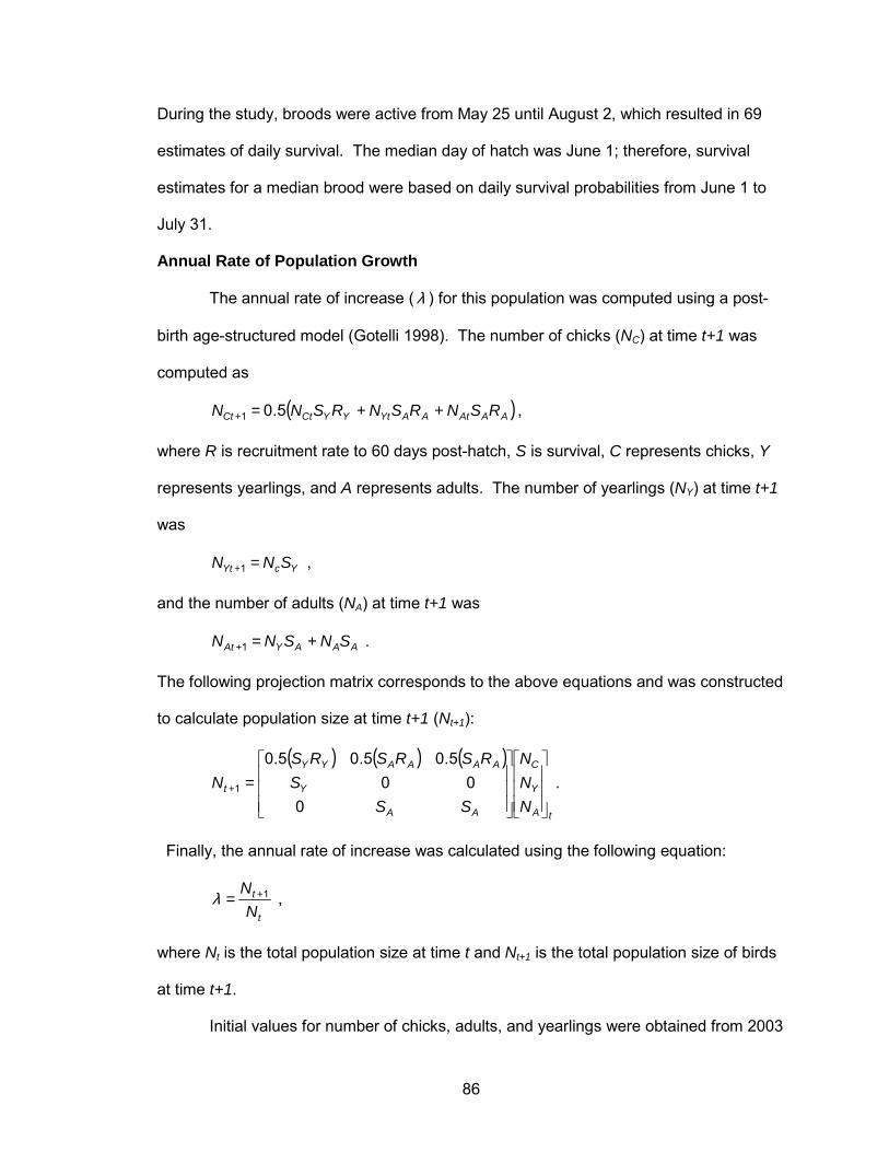
86

During the study, broods were active from May 25 until August 2, which resulted in 69

estimates of daily survival. The median day of hatch was June 1; therefore, survival

estimates for a median brood were based on daily survival probabilities from June 1 to

July 31.

Annual Rate of Population Growth

The annual rate of increase ( λ ) for this population was computed using a post-

birth age-structured model (Gotelli 1998). The number of chicks (NC) at time t+1 was

computed as

( )AAAtAAYtYYCtCt RSNRSNRSNN ++=+ 5.01 ,

where R is recruitment rate to 60 days post-hatch, S is survival, C represents chicks, Y

represents yearlings, and A represents adults. The number of yearlings (NY) at time t+1

was

YcYt SNN =+1 ,

and the number of adults (NA) at time t+1 was

AAAYAt SNSNN +=+1 .

The following projection matrix corresponds to the above equations and was constructed

to calculate population size at time t+1 (Nt+1):

( ) ( ) ( )

tA

Y

C

AA

Y

AAAAYY

t

NNN

SSS

RSRSRSN

=+

000

5.05.05.0

1 .

Finally, the annual rate of increase was calculated using the following equation:

t

t

NN 1+=λ ,

where Nt is the total population size at time t and Nt+1 is the total population size of birds

at time t+1.

Initial values for number of chicks, adults, and yearlings were obtained from 2003

87

data. Data from both years were used to calculate recruitment and survival rates.

Recruitment rates for yearlings and adults were estimated at 60 days post-hatch, which

typically corresponded to around July 31. Hens were censored from this estimate if

brood fates were unknown, their radio-collars failed prior to June 15, or they were

missing prior to June 15. Recruitment rates of 0.36 and 0.86 were used for yearlings

and adults, respectively.

Survival of yearlings from April 1 to July 31 was 0.70. This was estimated from

the present study using the best hen survival model. A rate of 0.61 was used for survival

of yearlings from August 1 through March 31. This survival probability was obtained

from a study in southwestern Kansas and it was calculated using a known fate model in

Program MARK (Pitman 2003). Adult survival from April 1 through September 30 was

0.56. This was estimated from the present study using the best hen survival model.

Survival probabilities for adults during August and September were assumed to be the

same as they were during the rest of the breeding season. A rate of 0.80 was used for

adult survival from October 1 to March 31. This survival rate was obtained from survival

probabilities of male lesser prairie-chickens in southwestern Kansas and it was

estimated using a joint live-recapture and band recovery model (Jamison 2000). Thus,

survival rates of 0.43 and 0.45 were used to compute the annual rate of population

growth ( λ ) for yearlings and adults, respectively.

RESULTS

Seventy-one females were captured and radio-collared during this two-year

study. Sixty nests were located by tracking transmitter-equipped birds. One 2002 nest

tended by a greater prairie-chicken was not included when calculating nest success and

modeling daily survival probabilities because the hen abandoned her nest shortly after

the first nest site visit by a researcher. Twenty-nine (48.3%) of these nests successfully

88

hatched > 1 chick. Out of the 29 nests that hatched, 27 broods were monitored during

this study.

Nesting Statistics

There was no evidence that the proportion of females that attempted incubation

differed between age classes or species (Table 3.2). However, there was a difference in

nesting rate between years with 73.7% of transmitter-equipped hens nesting in 2002 and

97.4% of transmitter-equipped hens nesting in 2003 (Table 3.3). There was evidence

that the mean incubation onset date for primary nest attempts was earlier for adults

compared to yearlings (Table 3.2). Renesting rates did not differ between age classes,

species, (Table 3.2) or years and 19.1% of females attempted a renest (Table 3.3).

Mean clutch size did not differ between age classes, species, (Table 3.2) or

years (Table 3.3). However, mean clutch size did vary between first and second nest

attempts (Table 3.2). Mean clutch size was 12.1 eggs for first nest attempts and 6.1

eggs for second nest attempts. Hatchability also did not differ between age classes,

species (Table 3.2), or years and the pooled estimate was 76.5% (Table 3.3). Apparent

nest success was 49.2% (Table 3.3).

Depredation accounted for 94% of nest failures. The primary nest predators

were coyotes (Canis latrans), striped skunks (Mephitus mephitus), and bull snakes

(Pituophis catenifer). Typically, mammals caused complete nest loss and snake

depredation resulted in partial nest loss. Other potential nest depredators included

spotted ground squirrels (Spermophilus spilosoma), thirteen-lined ground squirrels

(Spermophilus tridecemlineatus), chihuahuan ravens (Corvus cryptoleucus), and

badgers (Taxidea taxus) (Sargeant et al. 1998). Two nests also had ants depredate

eggs after chicks initiated pipping.

Brood Statistics

Twelve of the broods (44.4%) suffered compete losses of chicks prior to 14 days

89

post-hatch. The fate of two broods beyond 14 days of age was unknown. Six broods

(46.2%) suffered complete losses of chicks between 15 and 60 days post-hatch. Of the

25 broods that were tracked to 60 days post-hatch, only 7 broods (28.0%) were known

to have > 1 chick 60 days post-hatch. In addition to losses of entire broods, brood

flushes indicate a decline in the number of chicks per brood from hatch until 60 days

post-hatch (Table 3.4). The mean number of chicks that hatched per clutch was 9.6

chicks. The mean number of chicks per brood was 7.33 and 5.0 at 14 days and 60

days, respectively. Mean recruitment rate was 0.59 chicks per hen (95% CI = 0.49,

0.69).

Daily chick survival was estimated at 0.942 for pre-fledge broods (Table 3.5).

Daily chick survival and overall chick survival of chicks reared by adults were greater

than daily survival of chicks reared by yearlings (Table 3.5). Overall chick survival for

the pre-fledge period was 0.433 with estimates of 0.237 and 0.593 for yearlings and

adults, respectively (Table 3.5).

Estimates of daily chick survival were greater for post-fledge broods compared to

pre-fledge broods (Table 3.5). Overall daily chick survival was estimated at 0.979 for

post-fledge broods (Table 3.5). Chicks reared by adults had lower overall survival

compared to chicks reared by yearlings during post-fledge period (Table 3.5). Overall

post-fledge chick survival was higher during 2002 compared to 2003 with estimates of

0.952 for 2002 and 0.205 for 2003 (Table 3.5). Overall chick survival for post-fledge

broods was estimated at 0.372. There was a difference in overall survival from hatch to

60 days post-hatch between years. Chick survival from hatch to 60 days post-hatch was

estimated at 0.161 with estimates of 0.426 and 0.088 for 2002 and 2003, respectively.

Survival Analyses

Hens.--Sixty-nine hens were included within the hen survival analysis. Ninety-

three candidate models were used to evaluate the effects of eight sources of variation on

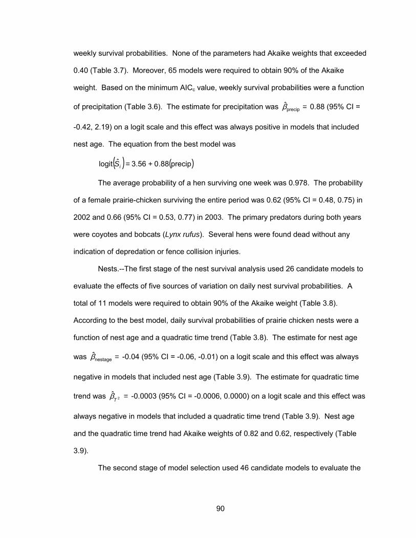
90

weekly survival probabilities. None of the parameters had Akaike weights that exceeded

0.40 (Table 3.7). Moreover, 65 models were required to obtain 90% of the Akaike

weight. Based on the minimum AICc value, weekly survival probabilities were a function

of precipitation (Table 3.6). The estimate for precipitation was =precip�β 0.88 (95% CI =

-0.42, 2.19) on a logit scale and this effect was always positive in models that included

nest age. The equation from the best model was

( ) ( )precip88.056.3�logit +=iS

The average probability of a hen surviving one week was 0.978. The probability

of a female prairie-chicken surviving the entire period was 0.62 (95% CI = 0.48, 0.75) in

2002 and 0.66 (95% CI = 0.53, 0.77) in 2003. The primary predators during both years

were coyotes and bobcats (Lynx rufus). Several hens were found dead without any

indication of depredation or fence collision injuries.

Nests.--The first stage of the nest survival analysis used 26 candidate models to

evaluate the effects of five sources of variation on daily nest survival probabilities. A

total of 11 models were required to obtain 90% of the Akaike weight (Table 3.8).

According to the best model, daily survival probabilities of prairie chicken nests were a

function of nest age and a quadratic time trend (Table 3.8). The estimate for nest age

was =nestage�β -0.04 (95% CI = -0.06, -0.01) on a logit scale and this effect was always

negative in models that included nest age (Table 3.9). The estimate for quadratic time

trend was =2�Tβ -0.0003 (95% CI = -0.0006, 0.0000) on a logit scale and this effect was

always negative in models that included a quadratic time trend (Table 3.9). Nest age

and the quadratic time trend had Akaike weights of 0.82 and 0.62, respectively (Table

3.9).

The second stage of model selection used 46 candidate models to evaluate the

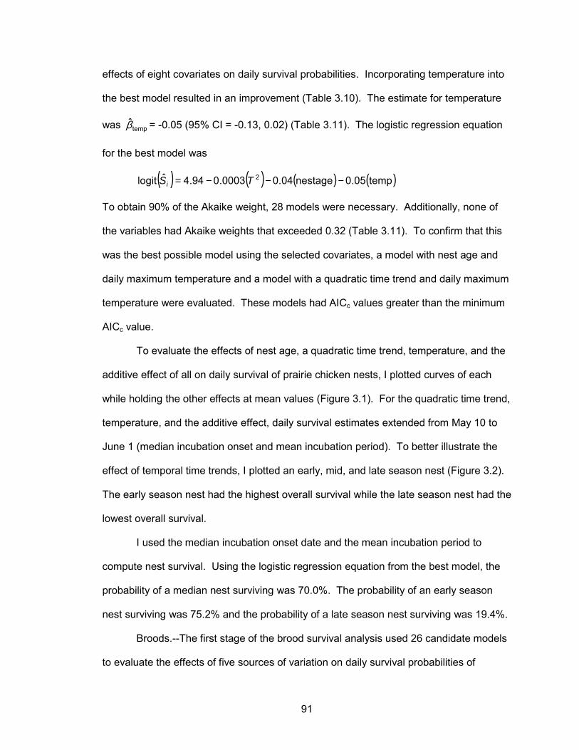
91

effects of eight covariates on daily survival probabilities. Incorporating temperature into

the best model resulted in an improvement (Table 3.10). The estimate for temperature

was temp�β = -0.05 (95% CI = -0.13, 0.02) (Table 3.11). The logistic regression equation

for the best model was

( ) ( ) ( ) ( )temp05.0nestage04.00003.094.4�logit 2 −−−= TSi

To obtain 90% of the Akaike weight, 28 models were necessary. Additionally, none of

the variables had Akaike weights that exceeded 0.32 (Table 3.11). To confirm that this

was the best possible model using the selected covariates, a model with nest age and

daily maximum temperature and a model with a quadratic time trend and daily maximum

temperature were evaluated. These models had AICc values greater than the minimum

AICc value.

To evaluate the effects of nest age, a quadratic time trend, temperature, and the

additive effect of all on daily survival of prairie chicken nests, I plotted curves of each

while holding the other effects at mean values (Figure 3.1). For the quadratic time trend,

temperature, and the additive effect, daily survival estimates extended from May 10 to

June 1 (median incubation onset and mean incubation period). To better illustrate the

effect of temporal time trends, I plotted an early, mid, and late season nest (Figure 3.2).

The early season nest had the highest overall survival while the late season nest had the

lowest overall survival.

I used the median incubation onset date and the mean incubation period to

compute nest survival. Using the logistic regression equation from the best model, the

probability of a median nest surviving was 70.0%. The probability of an early season

nest surviving was 75.2% and the probability of a late season nest surviving was 19.4%.

Broods.--The first stage of the brood survival analysis used 26 candidate models

to evaluate the effects of five sources of variation on daily survival probabilities of

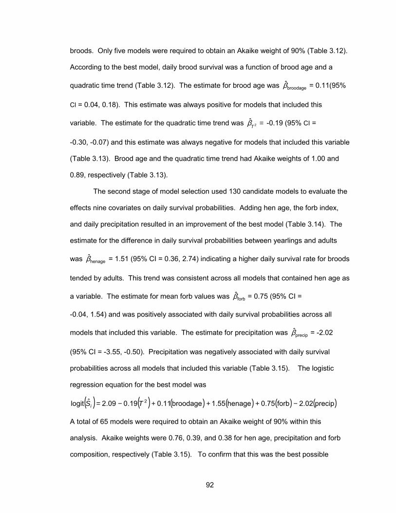
92

broods. Only five models were required to obtain an Akaike weight of 90% (Table 3.12).

According to the best model, daily brood survival was a function of brood age and a

quadratic time trend (Table 3.12). The estimate for brood age was broodage�β = 0.11(95%

Cl = 0.04, 0.18). This estimate was always positive for models that included this

variable. The estimate for the quadratic time trend was =2�Tβ -0.19 (95% CI =

-0.30, -0.07) and this estimate was always negative for models that included this variable

(Table 3.13). Brood age and the quadratic time trend had Akaike weights of 1.00 and

0.89, respectively (Table 3.13).

The second stage of model selection used 130 candidate models to evaluate the

effects nine covariates on daily survival probabilities. Adding hen age, the forb index,

and daily precipitation resulted in an improvement of the best model (Table 3.14). The

estimate for the difference in daily survival probabilities between yearlings and adults

was henage�β = 1.51 (95% CI = 0.36, 2.74) indicating a higher daily survival rate for broods

tended by adults. This trend was consistent across all models that contained hen age as

a variable. The estimate for mean forb values was forb�β = 0.75 (95% CI =

-0.04, 1.54) and was positively associated with daily survival probabilities across all

models that included this variable. The estimate for precipitation was precip�β = -2.02

(95% CI = -3.55, -0.50). Precipitation was negatively associated with daily survival

probabilities across all models that included this variable (Table 3.15). The logistic

regression equation for the best model was

( ) ( ) ( ) ( ) ( ) ( )precip02.2forb75.0henage55.1broodage11.019.009.2�logit 2 −+++−= TSi

A total of 65 models were required to obtain an Akaike weight of 90% within this

analysis. Akaike weights were 0.76, 0.39, and 0.38 for hen age, precipitation and forb

composition, respectively (Table 3.15). To confirm that this was the best possible

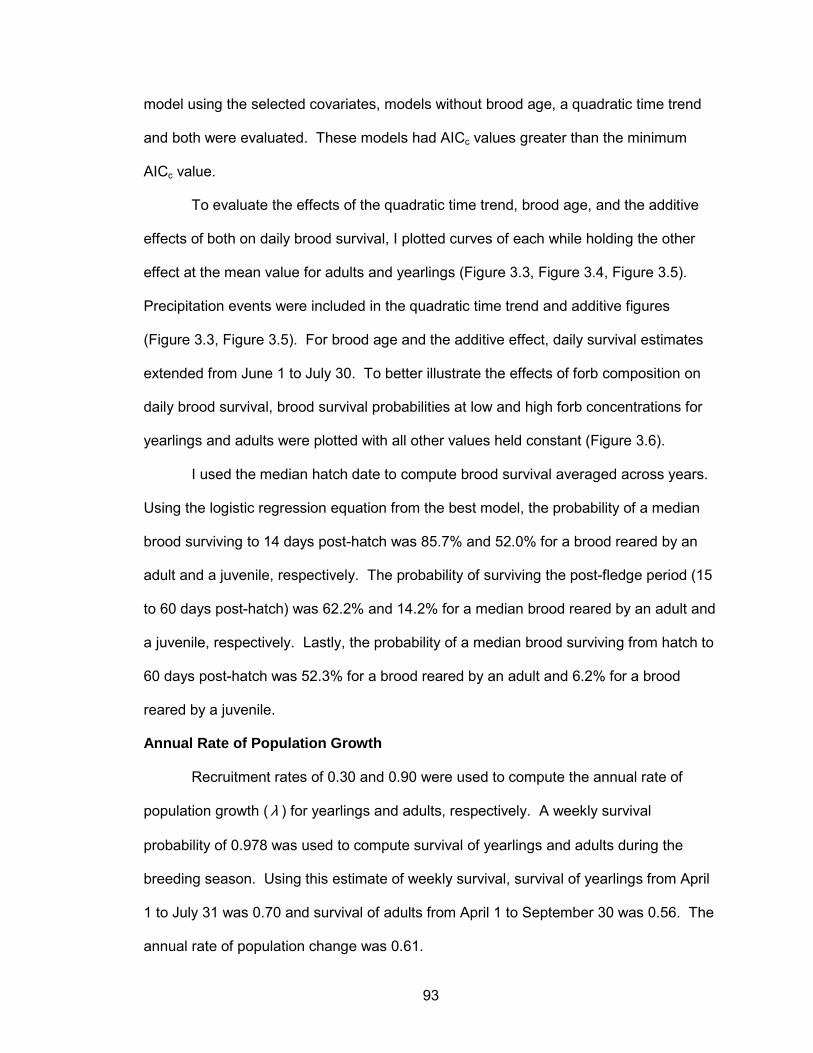
93

model using the selected covariates, models without brood age, a quadratic time trend

and both were evaluated. These models had AICc values greater than the minimum

AICc value.

To evaluate the effects of the quadratic time trend, brood age, and the additive

effects of both on daily brood survival, I plotted curves of each while holding the other

effect at the mean value for adults and yearlings (Figure 3.3, Figure 3.4, Figure 3.5).

Precipitation events were included in the quadratic time trend and additive figures

(Figure 3.3, Figure 3.5). For brood age and the additive effect, daily survival estimates

extended from June 1 to July 30. To better illustrate the effects of forb composition on

daily brood survival, brood survival probabilities at low and high forb concentrations for

yearlings and adults were plotted with all other values held constant (Figure 3.6).

I used the median hatch date to compute brood survival averaged across years.

Using the logistic regression equation from the best model, the probability of a median

brood surviving to 14 days post-hatch was 85.7% and 52.0% for a brood reared by an

adult and a juvenile, respectively. The probability of surviving the post-fledge period (15

to 60 days post-hatch) was 62.2% and 14.2% for a median brood reared by an adult and

a juvenile, respectively. Lastly, the probability of a median brood surviving from hatch to

60 days post-hatch was 52.3% for a brood reared by an adult and 6.2% for a brood

reared by a juvenile.

Annual Rate of Population Growth

Recruitment rates of 0.30 and 0.90 were used to compute the annual rate of

population growth ( λ ) for yearlings and adults, respectively. A weekly survival

probability of 0.978 was used to compute survival of yearlings and adults during the

breeding season. Using this estimate of weekly survival, survival of yearlings from April

1 to July 31 was 0.70 and survival of adults from April 1 to September 30 was 0.56. The

annual rate of population change was 0.61.

94

DISCUSSION

Low Akaike weights associated with the hen survival analysis (Table 3.6) indicate

that none of the models approximated weekly hen survival probabilities well. The level

of model selection uncertainty may be a result of reducing survival rates to weekly

estimates or poor selection of variables. The best model indicated that weekly survival

rates were positively associated with precipitation, which was contrary to what was

hypothesized. Condensing survival rates into weekly estimates may have masked the

negative effect of extreme daily precipitation events.

There are also limitations when including dominant habitat type as a variable

within the analysis. The dominant habitat type was included with the expectation that

habitat type would correspond to habitat quality. However, the dominant habitat type

was not the only habitat type used and survival may have depended on visitations to an

array of habitat types. Quantifying vegetation at hen locations may have better

represented habitat needs. I believe that the inclusion of the remaining variables was

reasonable.

The level of model uncertainty indicates that there may be covariates that better

represent weekly hen survival probabilities. The inclusion of a model that varied weekly

survival probabilities based on stage within the breeding season may have better

represented weekly hen survival probabilities. For example, models that varied weekly

survival probabilities across pre-nesting hens, nesting hens, post-nesting hens without

broods and post-nesting hens with broods may have predicted survival probabilities

better. Additionally, it was the intention of this study to include hen mass as a covariate

that reflected hen condition. However, hen mass varied depending on the date of

capture and species.

The probability of a hen surviving the breeding season was 0.62 and 0.66 in

95

2002 and 2003, respectively. This estimate is similar to estimates from other studies.

Survival of lesser prairie-chickens in southwestern Kansas from April 1st to September

30th was estimated at 0.74 over a three-year period and varied across months (Jamison

2000). Jamison (2000) roughly calculated survival of female lesser prairie-chickens from

another study in New Mexico during the breeding season. Survival was approximately

0.59 (Merchant 1982). Burger (1988) estimated survival for female greater prairie-

chickens in Missouri. Kaplan-Meier estimates ranged from 0.50 to 0.53 during pre-

nesting and nesting and from 0.69 to 0.79 during post-nesting, depending on the year.

The lower nesting rate in 2002 compared to 2003 may be a result of hen

condition. In New Mexico, a lower nesting rate during a drought year was attributed to

poor physiological condition (Merchant 1982). Merchant (1982) reported a nesting rate

of 92% during a spring of normal rainfall and a nesting rate of 73% during a drought

year. In a study performed by Dahlgren et al. (1990) on gray partridges, female diet

composition was directly correlated with the quality and quantity of eggs produced. The

primary dietary components of prairie chicken hens during this period include

invertebrates, especially grasshoppers, leaves, flowers, masts, and seeds (Davis et al.

1979). Dry springs, similar to the spring of 2002, can be detrimental to forbs and

grasses that grasshoppers and other invertebrates depend on (Eustace 2002).

Cumulative precipitation from April 15 to June 15, 2002 was only 5.99 cm, whereas

cumulative precipitation in 2003 was 16.03 cm for the same period (Figure 3.7).

The disparity in nesting rate between the two years of this study may also be a

result of temperature. Wilson (1949) reported that egg-laying decreased at

temperatures above 26.5C and some females ceased egg-laying after temperatures

exceeded 38C. The number of days between April 15 and June 15 that exceeded 26.5C

were 30 and 18 for 2002 and 2003, respectively (Figure 3.8). Thus, lack of spring rains

and high temperatures during 2002 may be responsible for the difference in nesting

96

rates between years. The nesting rate of lesser prairie-chickens in southwestern

Kansas was 92% across six years (Pitman 2003), which is similar to the pooled

estimated of 89.7% in the present study.

This is the first study that monitored both lesser and greater prairie-chicken nests

and broods within the same study area. Thus, there is no literature available that reports

nest and brood statistics of both prairie-chicken species occupying the same area.

Mean clutch size of both species was comparable to clutch sizes reported by other

studies. Mean clutch size was 11.2 with estimates of 11.9 and 10.2 for lesser prairie-

chickens and greater prairie-chickens, respectively (Table 3.2). Mean clutch size of

lesser prairie-chickens was 10.4 eggs with a range between 8 and 14 across 6 studies in

four states (Giesen 1998) and 12.0 for primary nest attempts in southwestern Kansas

(Pitman 2003). Mean clutch size of greater prairie-chickens across 13 studies in nine

states was 12.1 with a range of means between 10.0 and 14.3 (Peterson and Silvy

1996).

Mean egg hatchability was lower for greater prairie-chicken and lesser-prairie

chickens in this present study compared to other studies. Greater prairie-chicken egg

hatchability was only 65.0% during this study (Table 3.2) compared to 88.7% with a

range of 80.1% to 100.0% across 10 studies in seven states (Peterson and Silvy, 1996).

Lesser prairie-chicken egg hatchability was 83.6% (Table 3.2) compared to averages

greater than 90% for three studies in three states (Giesen 1998) and an average of

93.4% over six years in southwestern Kansas (Pitman 2003). The disparity between

egg hatchability is most likely due to differences in predator densities. Ninety-four

percent of the partial nest losses were attributed to snake depredation during this study.

Of the snake species known to depredate prairie-chicken nests, bull snakes were the

primary snake species within the study area.

The renesting rate was 19.1% (Table 3.3) with estimates of 30.0% for greater

97

prairie-chickens and 9.4% for lesser prairie-chickens (Table 3.2). This is lower than the

83% estimated for greater prairie-chickens in Minnesota (Svedarsky 1988) and the

31.3% renesting rate of lesser prairie-chickens in southwestern Kansas (Pitman 2003).

The energy lost during egg laying and incubation is substantial (Svedarsky 1979,

Bergerud and Gratson 1988). This, along with the effect of drought conditions on food

availability, may have resulted in hens in poor condition. Thus, renesting may have

been a poor option for hens.

According to the best nest survival model, daily survival probabilities were a

function of nest age, a quadratic time trend, and maximum daily temperature (Table

3.10). The low variable weight of temperature and model selection uncertainty within the

second stage of the nest analysis indicates that maximum temperature was not a good

predictor of nest survival (Table 3.10). The negative slope of nest age (Figure 3.1) was

attributed to an increase in scent trails to the nest as the age of the nest progresses.

Scent trails result from morning and evening feedings by the hen. Mammalian predators

use olfactory cues to locate nests (Roberts and Porter 1998) and 53.6% of complete

nest losses in this present study were attributed to mammals. Therefore, it is reasonable

to associate this mechanism with the decline in daily survival estimates as the nest ages.

The effects of temperature and the quadratic time trend were both negative

(Figure 3.1) indicating that early nests have the highest probability of survival. High

temperatures may affect nest attentiveness by requiring hens to move greater distances

in order to obtain food. When the female is absent, nests are more vulnerable to

predation and solar radiation (Merchant 1982). Temporal variation and temperature are

positively associated, which may have resulted in confounding. Adding temperature to

the model resulted in a decrease in the magnitude of the quadratic effect. Thus,

variation that was previously attributed to temporal trends was due to changes in

maximum daily temperature.

98

The remainder of the quadratic effect within the model may be due to

confounding with other weather variables. Gerstell (1936) documented the importance

of humidity in the artificial incubation of game bird nests. It was the intention of the

present study to include relative humidity within the analysis, but this variable was not

available at weather stations near the study area. The decline in daily survival

probabilities may also be a result of a decline in hen condition (Thogmartin and Johnson

1999) as the season progressed.

Using the equation from the best model, the probability of a median, early, and

late season nest surviving was 70.0%, 75.2%, 19.4%, respectively. However, literature

on nest survival is limited to estimates of apparent nest success and derived nest

survival estimates from this analysis are not comparable to other studies. Thus,

comparisons were done using apparent nest success. Apparent nest success for this

study was 49.2% (Table 3.3) with estimates of 54.3% and 41.7% for lesser prairie-

chickens and greater prairie-chickens, respectively (Table 3.2). A study performed in

southwestern Kansas between 1997 and 2002 calculated apparent nest success using

the Mayfield estimator. This study reported an overall nest success of 26.0%. The

higher nest success within the present study is most likely a function of habitat quality.

CRP provides nesting cover that is not typically found within the range of lesser prairie-

chickens.

Mean number of greater prairie-chicken chicks per brood at 14 days was 6.4 for

7 broods and mean number chicks per brood at 60 days post-hatch was 5.0 for three

broods in this study (Table 3.4). This is comparable to the average brood size of greater

prairie-chickens across six studies in Kansas from 1950 to 1968. The mean number of

chicks per broods prior to brood break-up in Kansas was 5.4 with a range of 2.0 to 7.3

and the mean number across 25 studies in 8 different states was 6.01 with a range of

2.0 to 7.7 (Peterson and Silvy 1996). Mean number of lesser prairie-chicken chicks per

99

brood at 14 days was 8.1 for 8 broods and mean number of chicks per brood at 60 days

post-hatch was 5.0 for four broods in this present study (Table 3.4). Average brood size

in July and August ranged from 3.27 to 3.67 in Kansas (Schwilling 1955, Jamison 2000),

between 5.2 and 7.5 in Oklahoma (Davison 1940, Copelin, 1963, Jones 1963) and 3.5

and 7.8 in New Mexico (Merchant 1982).

Daily prairie chicken chick survival was 0.942 and 0.979 for the pre-fledge and

post-fledge period, respectively. Overall chick survival was 0.433 for pre-fledge chicks,

0.372 for post-fledge chicks, and 0.161 for the entire 60-day period (Table 3.5). There is

no literature available on daily chick survival of greater prairie-chickens. Therefore,

comparisons are limited to literature on lesser prairie-chickens. Daily lesser prairie-

chicken chick survival was 0.938 and 0.975 for the pre-fledge and post-fledge period,

respectively. Overall chick survival was 0.411 for pre-fledge chicks, 0.308 for post-

fledge chicks, and 0.126 for the entire 60-day period (Table 3.5). Higher daily survival

rates during the post-fledge compared to pre-fledge period was also noted in

southwestern Kansas. Overall lesser prairie-chicken daily chick survival in

southwestern Kansas over six years was 0.949 for the pre-fledge period and 0.978 for

the post-fledge period (Pitman 2003). Similar to the present study, Pitman et al. (2003)

found higher chick survival for chicks reared by adults compared to yearlings during the

pre-fledge period and lower survival for chicks reared by adults compared to yearlings

during the post-fledge period. Overall chick survival estimates of 0.48 for pre-fledge

chicks, 0.37 for post-fledge chicks and 0.18 for the entire 60-day period (Pitman 2003)

were also comparable to estimates from this study. Four other studies have estimated

lesser prairie-chicken chick survival based on the size of broods in late summer

(Davison 1940, Schwilling 1955, Copelin 1963, Merchant 1982). A combined estimate

for these four studies is 0.31. However, these researchers failed to account for total

brood loss indicating that their estimates were probably biased high (Bergerud and

100

Gratson 1988).

There are several assumptions implicit in the daily chick survival estimates. First,

this method assumes that survival is constant across the period. This results in

homogeneous survival estimates. Therefore, daily survival rates are somewhat

inappropriate and overall survival rates are a more realistic representation of chick

survival. Second, it assumes that the fates of individual chicks are independent. This is

most likely violated because siblings are more likely to die from the same mortality

events. Violation of this assumption may cause little bias in survival estimates, but

results in underestimation of variances (Nichols et al. 1982, McCullagh and Nelder

1989). Third, it assumes that no brood mixing occurs.

According to the best brood survival model, daily survival probabilities were a

function of brood age, a quadratic time trend, hen age, forb composition, and

precipitation (Table 3.14). Low variable weights of forb composition and precipitation

and the level of model selection uncertainty within the second stage of the brood

analysis indicates that these variables were not good predictors of brood survival (Table

3.14). An increase in daily survival probabilities as the brood ages (Figure 3.4) is well

documented in the literature (Schwilling 1955, Ammann 1957, Bergerud and Gratson

1988). This relationship has been attributed to the acquisition of thermoregulatory and

flight abilities as the brood ages (Aulie 1976). The disparity between adult and yearling

reared broods (Figure 3.5) was most likely a result of experience.

The negative slope for the quadratic time trend (Figure 3.3) was most likely

confounded with weather variables. Spring and summer precipitation may indirectly

affect broods by influencing invertebrate production. Invertebrates provide essential

amino acids (methionine and cystine) that are not available in high concentrations within

vegetation (Wise 1982). These amino acids are critical to plumage development, which

is vital to chick thermoregulation and survival (Hurst 1972). Although hatches may

101

provide insects during the beginning of the brood-rearing season, dry summer conditions

negatively affect large nymph and adult stages (Kemp and Cigliano 1994). Total

precipitation during the brood-rearing season (May 25 to August 2) was only 4.80 cm

during 2002 and 7.47 cm during 2003 (Figure 3.7). From field observations, it was

evident that both seasons experienced a decline in grasshopper abundance throughout

the summer. This, compounded with the effects of low soil moisture on forbs and

grasses, may be detrimental to chick survival by decreasing invertebrate abundance

(Kemp and Cigliano 1994) and reducing cover (Hamerstrom and Hamerstrom 1968).

This suggests that invertebrates may have played a role in downward trend in daily

survival probabilities. Low relative humidity characteristic of summers with low rainfall

may also affect broods by increasing evaporation (Ahlborn 1980).

Summer temperatures may directly affect broods by inducing heat stress and

water loss (Merchant 1982). According to Aulie and Moen (1975) willow ptarmigan

chicks inside a 38.9C climactic chamber experienced an increase in body temperature to

41.5C after 20 minutes. An ambient temperature of 38.9C corresponds to an air

temperature of approximately 35C (Flanders 2002). Flanders (2002) also found that

number of June days exceeding 35C was negatively associated with sharp-tailed grouse

production. The number of days during the brood-rearing season exceeding 35C was

32 and 23 during 2002 and 2003, respectively and maximum temperature increased as

the season progressed (Figure 3.8). Behavioral responses of broods to high

temperatures may indirectly result in decreased survival by decreasing feeding time.

Lesser prairie-chickens are known to seek shade during periods of high temperatures

(Ahlborn 1980). The indirect and direct effects of high temperatures, along with the

effects of dry summer weather, may have resulted in a decline in daily brood survival

probabilities throughout the brood-rearing season. The failure of this analysis to reveal

the importance of these weather variables may be a result of the direct and indirect

102

effects of a combination of weather variables, the differing impacts of weather between

years, and the difficulty of representing the cumulative effects of weather across the

season. The complexity of these effects was better represented by a quadratic time

trend.

Using the equation from the best model, the probability of a median brood

surviving was 52.3% and 6.2% for a brood reared by an adult and juvenile, respectively.

However, literature on brood survival is limited to estimates of apparent success. Thus,

derived brood survival estimates from this analysis are not comparable to other studies.

Comparisons were done using apparent brood success. Only 6 out of 10 (60.0%)

greater prairie-chicken broods survived passed 14 days of age and only 3 out of 9

(33.3%) survived until 60 days of age in my study. Svedarsky (1988) reported that only

1 of 11 (9.0%) broods made it to 6 weeks of age in Minnesota. In contrast, a study in

Wyoming (Sheyenne National Grasslands) found that 13 of 22 (59.1%) broods survived

beyond 56 days of age (Newell 1988). Nine out of 17 lesser prairie-chicken broods

survived to 14 days post-hatch (52.9%) and 4 out of 16 (25.0%) survived to 60 days

post-hatch in the present study. A study in southwestern Kansas documented complete

loss of 33.3% (66.7% successful) of broods prior to 14 days post-hatch and 38.2%

(61.8% successful) of broods prior to 60 days post-hatch (Pitman 2003).

There are several assumptions underlying the survival analyses that warrant

discussion. The assumptions include: (1) fates of hens, nests, and broods are correctly

determined; (2) research procedures do not influence survival; (3) fates of hens, nests,

and broods are independent; and (4) individual homogeneity (Dinsmore et al. 2002).

Assumption one was not a problem for this study. Implicit in this assumption is that

relocation probabilities of hens were independent of survival. There were very few hens

that went missing during this study; therefore, this should not have biased estimates.

Assumption two may have been a problem for hens if radio-transmitters

103

influenced survival during this study. A number of studies have found no difference

between survival of transmitter-equipped birds compared to those without transmitters

(Hines and Zwickel 1985, Erikstad 1979, Herzog 1979), whereas a number of studies

have documented differential behavior and/or mortality of radio-marked birds (Boag

1972, Marks and Marks 1987). The impact of observer disturbance on nests was

thought to be minimal for the present study because nests were only visited once and

precautions were taken to minimize disturbance. Abandonment in this study occurred

on one occasion (1.7%), which is much lower than the 34.7% reported by Riley et al.

(1992). Skagen et al. (1999) noted that success of artificial nests with quail eggs in the

short-grass prairie of northeast Colorado was not negatively impacted by the presence

of human scent within three days of nest site visitation. This assumption was possibly

violated on one occasion; therefore, this nest attempt was eliminated from the survival

analysis. The impact of observer disturbance on broods was thought to be minimal for

this study because broods were only flushed three times.

Assumption three was not an issue because transmitter-equipped hens, nests,

and broods were not located near one another. Lastly, assumption four would be

violated if survival probabilities were a function of individual heterogeneity. This would

occur if certain hens, nests and broods were inherently more susceptible to mortality

(Dinsmore et al. 2002). In the nest and brood survival analyses, this would result in

indistinguishable effects of nest and brood age and individual heterogeneity (Dinsmore

et al. 2002). Nest and brood age may have also been confounded by temporal variation,

but this is unlikely because nesting attempts and brood-rearing were spread out across

the nesting season.

Although there was no evidence that survival probabilities were a function of

habitat, the long-term benefit of CRP was evident. From field observations it was

apparent that CRP may be allowing these birds to persist in dry years. In contrast,

104

rangeland may be adequate when drought and the compounding effects of grazing do

not decrease critical nesting cover. The benefit of CRP was represented by the lack of a

difference in nest survival between years. The area experienced dry weather during

nesting in 2002 and wet weather during nesting in 2003. The only successful nests in

2002 were located in CRP, whereas successful nests were found in both CRP and

rangeland during 2003. A study in New Mexico on lesser prairie-chickens attributed the

absence of successful nests to drought and the subsequent deficiency of nesting cover

on rangelands (Wilson 1982). Additionally, the only two broods that survived beyond 14

day post-hatch in 2002 were located within ICRP at least 25% of the time. These

relationships may have been revealed if a year by habitat interaction, along with a larger

sample size, was included.

The annual rate of population growth for the two years of this study was

estimated to be 0.61. This indicates that this population is declining if these years are

representative of population trends. Analyses from this study suggest that low chick and

brood survival may be limiting this population. Increasing recruitment from 0.59 chicks

per hen to 2.7 chicks per hen would result in an annual rate of population growth greater

than one. Fortunately, lack of precipitation and high temperatures during the two

summers of my study indicates that chick and brood survival during these two years may

represent the low end for this population.


The survival analysis indicated that nesting early in the season is crucial to the

persistence of prairie chickens in this area. Management that provides food sources

during the spring may increase the number of hens that initiate nests early. In addition

to increasing the percentage of interseeded CRP, food plots within ICRP may benefit

prairie chicken hens. According to Bidwell et al. (2002), food plots should be larger than

105

4 ha in size and placed within good quality habitat away from trees or power lines.

However, interseeding is the preferred management option on CRP fields due to the

potential of food plots to attract predators (Bidwell et al. 2002). Improving the quality of

crop fields may increase the number of hens that initiate nests early. Conservation

tillage could be practiced on crop fields to leave residual cover and increase food

availability. Planting native grass and forb terraces may also increase the value crop

fields to prairie chickens by increasing escape cover in close proximity to food sources

(Bidwell et al. 2002). Forbs should be integrated into grass terraces because of their

value as a substrate to invertebrates.

Management strategies that protect important nesting habitat from disturbance

from May 1 to June 15 are essential. Moreover, retaining tall grass cover during this

period is critical. This means that timing of prescribed burns, haying, and mowing

should be carefully planned as not to influence cover during nesting. Landowners in

west central Kansas should be encouraged to implement a grazing regime that

increases vegetative cover on a portion of their land. Increasing the availability of CRP

may also help maintain the prairie-chicken population by providing a refuge habitat for

nesting in dry years.

Low chick survival, brood survival, and low recruitment to 60 days post-hatch

indicate that brood-rearing is the most critical period for this population. Therefore,

improving chick and brood survival should be a primary goal for the management of

prairie chickens in this area. Enhancing invertebrate production by increasing the

abundance of forbs should be emphasized. In addition to interseeding, strip disking, and

burning are other methods effective at increasing forb abundance on CRP fields (Hurst

1972, Buckner and Landers 1979, Landers and Mueller 1986, Manley et al. 1994,

Bidwell et al. 2002). Litton et al. (1994) recommended strip-disking at depths of 7 to 15

cm during March. According to Kirsch (1974), prescribed burning is the most effective

106

method for maintaining prairie chicken nesting and brood-rearing habitat. In Kansas,

burned areas had a greater variety of insects compared to unburned areas (Queal

1973). Increased invertebrate biomass, especially grasshoppers, and increased fruit

and seed production were observed on burned areas in North Dakota (Kirsch and Kruse

1973). Management used to increase the abundance of forbs should be implemented at

three to five-year intervals on 20 to 30% of the management unit during late summer, fall

or winter (Kirsch 1974, Bidwell 2002).

The survival analysis and daily chick survival estimates indicated that survival

during the first 14 to 20 days post-hatch is the lowest. The survival analysis also

suggested that early hatches are important due to the decline in brood survival as the

season progresses. Ninety-two percent of primary nest attempts hatched between May

25 and June 15, indicating that May 25 to July 5 encompass the most sensitive period in

regards to brood age. Rangelands, CRP, and croplands were all important habitats of

hens with broods. Therefore, minimizing disturbance and maintaining cover and food

within these habitat types and time frames is critical. Additionally, the combination of

brood age and a quadratic time trend resulted in low daily survival towards the end of the

brood-rearing season. This was attributed to heat stress and the response of vegetation

and invertebrates to lack of precipitation. Therefore, maintaining cover and forbs on

rangelands and CRP is also critical during the latter half of the brood-rearing season.

LITERATURE CITED

Ahlborn, G. G. 1980. Brood-rearing habitat and fall-winter movements of lesser prairie chickens in eastern New Mexico. Thesis, New Mexico State University, Las Cruces, New Mexico, USA.

Akaike, H. 1973. Information theory as an extension of the maximum likelihood

principle. Pages 267-281 in B. N. Petrov, and F. Csaki, editors. Second International Symposium on Information Theory. Akademiai Kiado, Budapest.

Ammann, G. A. 1957. The prairie grouse of Michigan. Technical Bulletin Project W-

070-R. Michigan Department of Conservation, Lansing, MI, USA.

107


Rangelands 20:13-16. Aulie, A. 1976. The pectoral muscles and the development of thermoregulation in

chicks of willow ptarmigan (Lagopus lagopus). Comparative Biochemistry and Physiology 53:343-346.

_____, and P. Moen. 1975. Metabolic thermoregulatory responses in eggs and chicks

of willow ptarmigan (Lagopus lagopus). Comparative Biochemistry and Physiology 51:605-609.

Bergerud A. T., and M. W. Gratson. 1988. Adaptive strategies and population ecology

of northern grouse. Volume 2. University of Minnesota Press. Minneapolis, Minnesota, USA.

Bidwell, T. G, S. D. Fuhlendorf, B. Gillen, S. Harmon, R. Horton, R. D. Rodgers, S.


Boag, D. A. 1972. Effect of radio packages on behavior of captive red grouse. Journal

of Wildlife Management 36:511-518. Boggs, C. E., E. Norris, and J. B. Steen. 1977. Behavioural and physiological

temperature regulation in young chicks of the willow grouse (Lagopus lagopus). Comparative Biochemistry and Physiology. Part A: Comparative Physiology 58:371-372.


food plants and seed supplies. Journal of Wildlife Management 43:807-811. Burger, L. W. Jr. 1988. Movements, home range, and survival of female greater prairie-

chickens in relation to habitat pattern. Thesis, University of Missouri, Columbia, Missouri, USA.

_____, Kurzejeski, T. V. Dailey, and M. R. Ryan. 1993. Relative invertebrate

abundance and biomass in Conservation Reserve Program plantings in Northern Missouri. Pages 102-108 in K. E. Church and T. V. Dailey, editors. Quail III: national quail symposium. Kansas Department of Wildlife and Parks, Pratt, Kansas, USA.

Burnham, K. P., and D. R. Anderson. 2002. Model selection and multimodel inference:

a practical information-theoretic approach. Second edition. Springer-Verlag, New York, New York, USA.

Candelaria, M. A. 1979. Movements and habitat-use by lesser prairie chickens in

eastern New Mexico. Thesis, New Mexico State University, Las Cruces, New Mexico, USA.

Copelin, F. F. 1963. The lesser prairie chicken in Oklahoma. Oklahoma Wildlife

108

Conservation Department, Oklahoma City, Oklahoma, USA. Crawford, J. A. 1980. Status, problems, and research needs of the lesser prairie

chicken. Pages 1-7 in P. A. Vohs and F. L. Knopf, editors. Proceedings of the Prairie Grouse Symposium. Oklahoma State University, Stillwater, Oklahoma, USA.

Dahlgren, J. 1990. The significance of arthropods in the gray partridge diet. Pages

202-213 in K. E. Church and S. J. Brady, editors. Perdix V: gray partridge and ring-necked pheasant workshop. Kansas Department of Wildlife and Parks, Emporia, Kansas, USA.

Daubenmire, R. 1959. A canopy-coverage method of vegetational analysis. Northwest

Science 33:43-64. Davis, C. A., T. Z. Riley, R. A. Smith, H. R. Suminski, and M. J. Wisdom. 1979. Habitat

evaluation of lesser prairie chickens in eastern Chaves County, New Mexico. New Mexico Agriculture Experimental Station, Las Cruces, New Mexico, USA.

_____, _____, _____, and M. J. Wisdom. 1980. Spring-summer food of lesser prairie

chicken in New Mexico. Pages 75-80 in P. A. Vohs, Jr. and F. L Knopf, editors. Proceedings of the Prairie Grouse Symposium. Oklahoma State University, Stillwater, OK, USA.

Davison, V. E. 1940. An 8-year census of lesser prairie-chickens. Journal of Wildlife

Management 4:55-62. Dinsmore, S. J., G. C. White, and F. L. Knopf. 2002. Advanced techniques for modeling

avian nest survival. Ecology 83:3476-3488. Doerr, T. B., and F. S. Guthery. 1983. Food selection by lesser prairie chickens in

northwest Texas. Southwest Naturalist 28:381-383. Erikstad, K. E. 1979. Effects of radio packages on reproductive success of willow

grouse. Journal of Wildlife Management 43:170-175. _____. 1985. Growth and survival of willow grouse chicks in relation to home range

size, brood movements, and habitat selection. Ornis Scandinavica 14:249-252. _____, and R. Andersen. 1983. The effect of weather on survival, growth rate and

feeding time in different sized willow grouse broods. Ornis Scandinavica 14:249-252.

_____, and T. K. Spidso. 1982. The influence of weather on food intake, insect prey

selection and feeding behaviour in willow grouse chicks in northern Norway. Ornis Scandinavica 13:176-182.

Eustace, C. D. 2002. Sage grouse hatching success and chronology for south-central

Montana. Intermountain Journal of Sciences 8:82-93. Flanders, B. L. 2002. Prairie grouse production on Valentine National Wildlife Refuge:

109

The effects of weather and grassland management. Thesis, Colorado State University, Fort Collins, Colorado, USA.

Forrester, N. D., F. S. Guthery, S. D. Kopp, and W. E. Cohen. 1998. Operative

temperature reduces habitat space for northern bobwhites. Journal of Wildlife Management 62:1506-1511.

Gerstell, R. C. 1936. Precipitation in relation to game crops. American Wildlife 25:26-

28. Gibbons, J. W., and R. D. Semlitsch. 1987. Activity patterns. Pages 396-421 in R. A.

Seigel, J. T. Collins, and S. S. Novak, editors. Snakes: ecology and evolutionary biology. Macmillan, New York, New York, USA.

Giesen, K. M. 1994. Breeding range and population status of lesser prairie-chickens in

Colorado. Prairie Naturalist 26:175-182. _____. 1998. Lesser prairie chicken. Pages 1-19 in A. Poole and F. Gille, editors. The

Birds of North America No. 364. The birds of North America, Inc., Philadelphia, Pennsylvania, USA.

Gotelli, N. J. 1998. A primer in ecology. 2nd. ed. Sinauer Associates, Sunderland,

Massachusetts, USA. Guthery, F. S., C. L. Land, and B. W. Hall. 2001. Heat loads on reproducing bobwhites

in the semiarid subtropics. Journal of Wildlife Management 65:111-117. Hamerstrom, F. N., Jr., and F. Hamerstrom. 1968. Water and the prairie chickens.

Wisconsin Academic Review 16:33-34. Herzog, P.W. 1979. Effects of radio-marking on behavior, movements, and survival of

spruce grouse. Journal of Wildlife Management 43:316-323. Hines, J. E., and F. C. Zwickel. 1985. Influence of radio packages on young blue

grouse. Journal of Wildlife Management 49:1050-1054. Horak, G. J., and R. D. Applegate. 1999. Greater prairie chicken management. Kansas

School Naturalist 45:3-15. Huakos, D. A., and L. M. Smith. 1989. Lesser prairie-chicken nest site selection and

vegetation characteristics in tebuthiuron-treated and untreated sand shinnery oak in Texas. Great Basin Naturalist 49: 624-626.


A. Morrison and L. C. Lewis, editors. Proceedings of the first National Bobwhite Quail Symposium, Oklahoma State University, Stillwater, Oklahoma, USA.

Jamison, B. E. 2000. Lesser prairie chicken chick survival, adult survival, and habitat

selection and movements of females in fragmented rangelands of southwestern Kansas. Thesis, Kansas State University, Manhattan, Kansas, USA.

110

Jensen, W. E., D. A. Robinson, and R. D. Applegate. 2000. Distribution and population trends of lesser prairie-chickens in Kansas. Prairie Naturalist 32:169-176.


habitat. Journal of Wildlife Management 27:757-778. Kemp, W. P., and M. M. Cigliano. 1994. Drought and rangeland grasshopper species

diversity. Canadian Entomologist 126:1075-1092. Kirsch, L. M. 1974. Habitat management considerations for prairie chickens. Wildlife

Society Bulletin 2:125-129. _____, and A. D. Kruse. 1973. Prairie fires and wildlife. Proceedings of the Tall

Timbers Fire Ecology Conference 12:289-303. Landers, J. L., and B. S. Mueller. 1986. Bobwhite quail management: a habitat


Litton, G., R. L.West, D. F. Dvorak, and G. T. Miller. 1994. The lesser prairie chicken


Manley, S. W., R. S. Fuller, J. M. Lee, and L. A. Brennan. 1994. Arthropod response to


Marks, J. S., and V. S. Marks. 1987. Influence of radio collars on survival of sharp-

tailed grouse. Journal of Wildlife Management 51:468-471. Mayfield, H. F. 1975. Suggestions for calculating nest success. Wilson Bulletin 87:456-

466. McCullagh, P., and J. A. Nelder. 1989. Generalized linear models, second edition.

Chapman and Hall, New York, New York, USA. Merchant, S. S. 1982. Habitat-use, reproductive success, and survival of female lesser

prairie chickens in two years of contrasting weather. Thesis, New Mexico State University, Las Cruces, New Mexico, USA.

Newell, J. N. 1988. Nesting and brood rearing ecology of the greater prairie chicken in

the Sheyenne National Grasslands, North Dakota. Thesis, Montana State University, Bozeman, Montana, USA.

Nichols, J. D., S. L. Stokes, J. E. Hines, and M. J. Conroy. 1982. Additional comments

on the assumption of homogeneous survival rates in modern bird banding estimation models. Journal of Wildlife Management 46:953-962.

Offerdahl, S. D., and A. J. Fivizzani. 1987. The development of thermoregulation in

gray partridge chicks. Pages 125-128 in R. O. Kimmel, J. W. Wchultz, and G. J.

111

Mitchell, editors. Proceedings of Perdix IV: Gray Partridge Workshop. Minnesota Department of Natural Resources, St. Paul, Minnesota, USA.

Palmer, W. E., G. A. Hurst, J. E. Stys, D. R. Smith, and J. D. Burk. 1993. Survival rates

of wild turkey hens in loblolly pine plantations in Mississippi. Journal of Wildlife Management 57:783-789.

Park, K. J., P. A. Robertson, S. T. Campbell, R. Foster, Z. M. Russell, D. Newborn, and

P. J. Hudson. 2001. The role of invertebrates in the diet, growth, and survival of red grouse (Lagopus lagopus scoticus) chicks. Journal of Zoology 254:137-145.

Pedersen, H. C., and J. B. Steen. 1979. Behavioural thermoregulation in willow

ptarmigan chicks (Lagopus lagopus). Ornis Scandinavica 10:17-21. Peterson, M. J., and N. J. Silvy. 1996. Reproductive stages limiting productivity of the

endangered attwater�s prairie chicken. Conservation Biology 10: 1264-1276. Pitman, J. C. 2003. Lesser prairie-chicken nest site selection and nest success,

juvenile gender determination and growth, and juvenile survival and dispersal in southwestern Kansas. Thesis, Kansas State University, Manhattan, Kansas, USA.

Queal, L. M. 1973. Fire � tool or tyrant. Kansas Game and Fish 30:7-9. Riley, T. Z. 1978. Nesting and brood-rearing habitat of lesser prairie chickens. Thesis,

New Mexico State University, Las Cruces, New Mexico, USA. ____, and C. A. Davis. 1993. Vegetative characteristics of lesser prairie-chicken brood

foraging sites. The Prairie Naturalist 25:243-248. _____, _____, M. Ortiz, and M. J. Wisdom. 1992. Vegetative Characteristics of

successful and unsuccessful nests of lesser prairie chickens. Journal of Wildlife Management 56: 383-387.

Robel, R. J., J. N. Briggs, A.D. Dayton, and L.C. Hulbert. 1970. Relationships between

visual obstruction measurements and weight of grassland vegetation. Journal of Range Management 23:295-297.

Roberts, S. D., and W. F. Porter. 1998. Relation between weather and survival of wild

turkey nests. Journal of Wildlife Management 62:1492-1498. _____, J. M. Coffey, and W. F. Porter. 1995. Survival and reproduction of female wild

turkeys in New York. Journal of Wildlife Management 59:437-447. Ryan, M. R., L. W. Burger Jr., D. P. Jones, and A. P. Wywialowski. 1998. Breeding

ecology of greater prairie-chickens (Typanuchus cupido) in relation to prairie landscape configuration. American Midland Naturalist 140:111-121.


Cary, North Carolina. 846pp.

112

Sargeant, A. B., M. A. Sovada, and R. J. Greenwood. 1998. Interpreting evidence of depredation of duck nests in the prairie pothole region. U. S. Geological Survey, Northern Prairie Wildlife Research Center, Jamestown, North Dakota, USA and Ducks Unlimited, Inc., Memphis, Tennessee, USA.

Schwilling, M. 1955. Study of lesser prairie chicken in southwest Kansas. Kansas Fish

and Game 12:10-12. Sell, D. L. 1979. Spring and summer movements and habitat use by lesser prairie

chicken females in Yoakum County, Texas. Thesis, Texas Tech. University, Lubbock, Texas, USA.

Skagen, S. K., T. R. Stanley, and M. B. Dillon. 1999. Do mammalian nest predators

follow human scent trails in the shortgrass prairie? Wilson Bulletin 111:415-420. Southwood, T. R. E., and D. J. Cross. 1963. The Ecology of the Partridge III. Breeding


Svedarsky, W. D. 1979. Spring and summer ecology of female greater prairie chickens

in northwestern Minnesota. Dissertation, University of North Dakota, Grand Forks, ND, USA.

_____. 1988. Reproductive ecology of female greater prairie chickens in Minnesota.

Pages 193-239 in A. T. Bergerud and M. W. Gratson, editors. Adaptive strategies and population ecology of northern grouse. Volume 2. University of Minnesota Press. Minneapolis, Minnesota, USA.

Taylor, M. A., and F. S. Guthery. 1980. Status, ecology, and management of the lesser

prairie chicken. General Technical Report RM-77. United States Department of Agriculture, National Forest Service, Fort Collins, Colorado, USA.

Thogmartin, W. E., and J. E. Johnson. 1999. Reproduction in a declining population of

wild turkeys in Arkansas. Journal of Wildlife Management 63:1281-1290. U. S. Department of the Interior. 2002. Endangered and threatened wildlife and plants;

12-month finding to list the lesser prairie-chicken as threatened and designate critical habitat. Federal Register 67:40657-40679.

Wallestad, R.O., and R. C. Watts. 1972. Small game research: factors affecting

annual sage grouse production in central Montana. Montana Department of Fish and Game, Helena, Montana, USA.

White, G. C., and K. P. Burnham. 1999. Program MARK: survival estimation from

populations of marked animals. Bird Study 46:S120-139. Wilson, W. O. 1949. High environmental temperatures as affecting the reaction of

laying hens to iodized casein. Poultry Science 28:581-592. Wilson, D. L. 1982. Nesting Habitat of Lesser Prairie Chickens in Roosevelt and Lea

Counties, New Mexico. Thesis, New Mexico State University, Las Cruces, New

113

Mexico, USA. Wisdom, M. J. 1980. Nesting habitat of lesser prairie chickens in eastern New Mexico.

Thesis, University of New Mexico, Las Cruces, New Mexico, USA. Wisdom, M. L., and L. S. Mills. 1997. Sensitivity analysis to guide population recovery:

prairie-chickens as an example. Journal of Wildlife Management 61:302-312. Wise, D. R. 1982. Nutrition of wild red grouse (Lagopus lagopus scoticus). Ibis 119:1-

9.

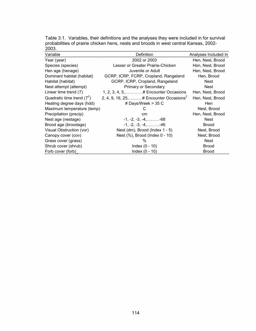
114

Table 3.1. Variables, their definitions and the analyses they were included in for survival probabilities of prairie chicken hens, nests and broods in west central Kansas, 2002-2003. Variable Definition Analyses Included InYear (year) 2002 or 2003 Hen, Nest, Brood Species (species) Lesser or Greater Prairie-Chicken Hen, Nest, Brood Hen age (henage) Juvenile or Adult Hen, Nest, Brood Dominant habitat (habitat) GCRP, ICRP, FCRP, Cropland, Rangeland Hen, Brood Habitat (habitat) GCRP, ICRP, Cropland, Rangeland Nest Nest attempt (attempt) Primary or Secondary Nest Linear time trend (T) 1, 2, 3, 4, 5,��.# Encounter Occasions Hen, Nest, Brood Quadratic time trend (T2) 2, 4, 9, 16, 25,��.# Encounter Occasions2 Hen, Nest, Brood Heating degree days (hdd) # Days/Week > 35 C Hen Maximum temperature (temp) C Nest, Brood Precipitation (precip) cm Hen, Nest, Brood Nest age (nestage) -1, -2, -3, -4,��-68 Nest Brood age (broodage) -1, -2, -3, -4,��-46 Brood Visual Obstruction (vor) Nest (dm), Brood (Index 1 - 5) Nest, Brood Canopy cover (cov) Nest (%), Brood (Index 0 - 10) Nest, Brood Grass cover (grass) % Nest Shrub cover (shrub) Index (0 - 10) Brood Forb cover (forb)_ Index (0 - 10) Brood

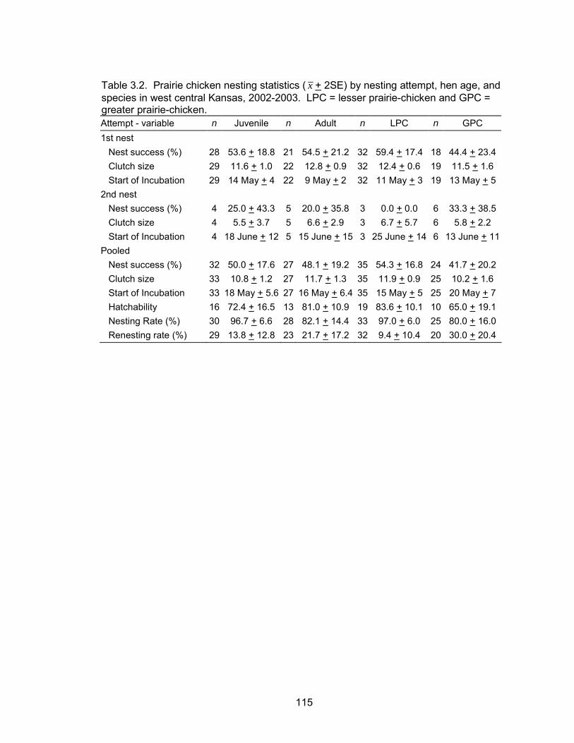
115

Table 3.2. Prairie chicken nesting statistics ( x + 2SE) by nesting attempt, hen age, and species in west central Kansas, 2002-2003. LPC = lesser prairie-chicken and GPC = greater prairie-chicken. Attempt - variable n Juvenile n Adult n LPC n GPC 1st nest Nest success (%) 28 53.6 + 18.8 21 54.5 + 21.2 32 59.4 + 17.4 18 44.4 + 23.4 Clutch size 29 11.6 + 1.0 22 12.8 + 0.9 32 12.4 + 0.6 19 11.5 + 1.6 Start of Incubation 29 14 May + 4 22 9 May + 2 32 11 May + 3 19 13 May + 5 2nd nest Nest success (%) 4 25.0 + 43.3 5 20.0 + 35.8 3 0.0 + 0.0 6 33.3 + 38.5 Clutch size 4 5.5 + 3.7 5 6.6 + 2.9 3 6.7 + 5.7 6 5.8 + 2.2 Start of Incubation 4 18 June + 12 5 15 June + 15 3 25 June + 14 6 13 June + 11Pooled Nest success (%) 32 50.0 + 17.6 27 48.1 + 19.2 35 54.3 + 16.8 24 41.7 + 20.2 Clutch size 33 10.8 + 1.2 27 11.7 + 1.3 35 11.9 + 0.9 25 10.2 + 1.6 Start of Incubation 33 18 May + 5.6 27 16 May + 6.4 35 15 May + 5 25 20 May + 7 Hatchability 16 72.4 + 16.5 13 81.0 + 10.9 19 83.6 + 10.1 10 65.0 + 19.1 Nesting Rate (%) 30 96.7 + 6.6 28 82.1 + 14.4 33 97.0 + 6.0 25 80.0 + 16.0 Renesting rate (%) 29 13.8 + 12.8 23 21.7 + 17.2 32 9.4 + 10.4 20 30.0 + 20.4

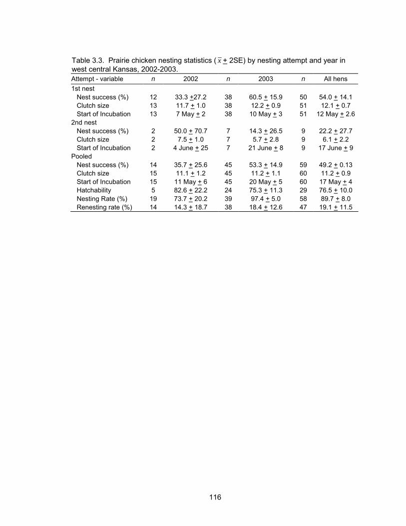
116

Table 3.3. Prairie chicken nesting statistics ( x + 2SE) by nesting attempt and year in west central Kansas, 2002-2003. Attempt - variable n 2002 n 2003 n All hens 1st nest Nest success (%) 12 33.3 +27.2 38 60.5 + 15.9 50 54.0 + 14.1 Clutch size 13 11.7 + 1.0 38 12.2 + 0.9 51 12.1 + 0.7 Start of Incubation 13 7 May + 2 38 10 May + 3 51 12 May + 2.62nd nest Nest success (%) 2 50.0 + 70.7 7 14.3 + 26.5 9 22.2 + 27.7 Clutch size 2 7.5 + 1.0 7 5.7 + 2.8 9 6.1 + 2.2 Start of Incubation 2 4 June + 25 7 21 June + 8 9 17 June + 9 Pooled Nest success (%) 14 35.7 + 25.6 45 53.3 + 14.9 59 49.2 + 0.13 Clutch size 15 11.1 + 1.2 45 11.2 + 1.1 60 11.2 + 0.9 Start of Incubation 15 11 May + 6 45 20 May + 5 60 17 May + 4 Hatchability 5 82.6 + 22.2 24 75.3 + 11.3 29 76.5 + 10.0 Nesting Rate (%) 19 73.7 + 20.2 39 97.4 + 5.0 58 89.7 + 8.0 Renesting rate (%) 14 14.3 + 18.7 38 18.4 + 12.6 47 19.1 + 11.5

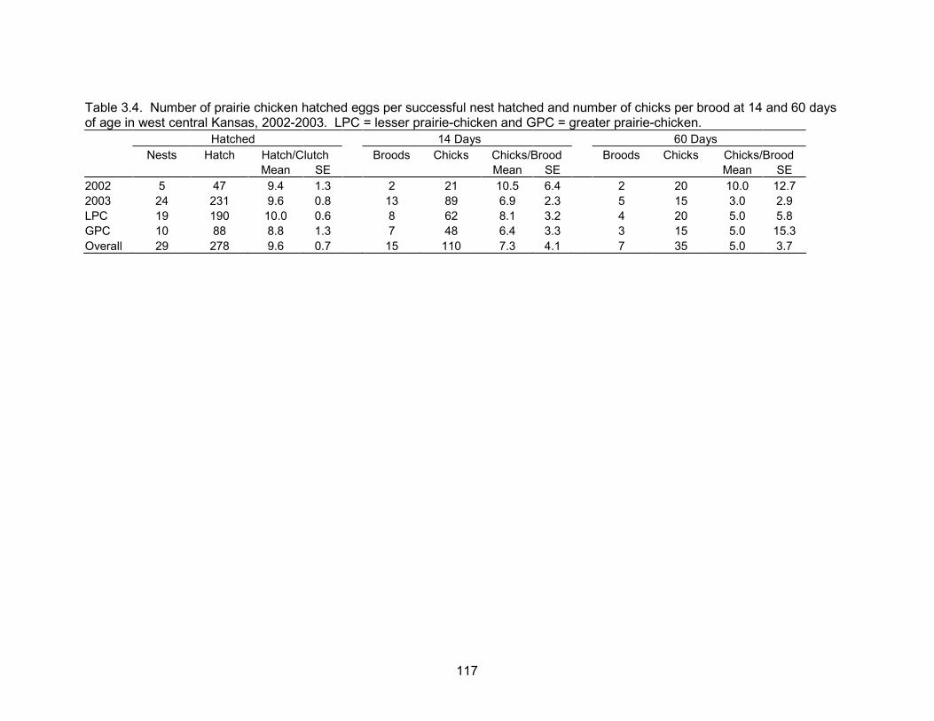
117

Table 3.4. Number of prairie chicken hatched eggs per successful nest hatched and number of chicks per brood at 14 and 60 days of age in west central Kansas, 2002-2003. LPC = lesser prairie-chicken and GPC = greater prairie-chicken. Hatched 14 Days 60 Days Nests Hatch Hatch/Clutch Broods Chicks Chicks/Brood Broods Chicks Chicks/Brood Mean SE Mean SE Mean SE 2002 5 47 9.4 1.3 2 21 10.5 6.4 2 20 10.0 12.7 2003 24 231 9.6 0.8 13 89 6.9 2.3 5 15 3.0 2.9 LPC 19 190 10.0 0.6 8 62 8.1 3.2 4 20 5.0 5.8 GPC 10 88 8.8 1.3 7 48 6.4 3.3 3 15 5.0 15.3 Overall 29 278 9.6 0.7 15 110 7.3 4.1 7 35 5.0 3.7

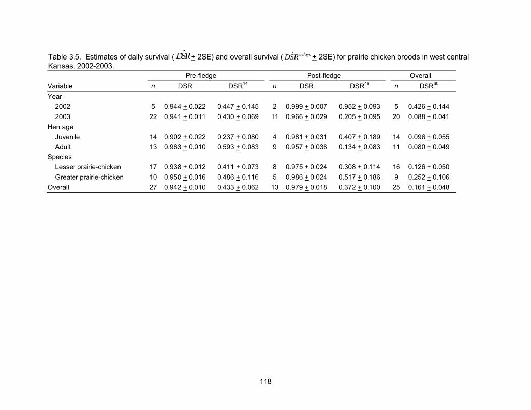
118

Table 3.5. Estimates of daily survival ( RSD� + 2SE) and overall survival ( daysRSD #� + 2SE) for prairie chicken broods in west central Kansas, 2002-2003. Pre-fledge Post-fledge Overall Variable n DSR DSR14 n DSR DSR46 n DSR60 Year 2002 5 0.944 + 0.022 0.447 + 0.145 2 0.999 + 0.007 0.952 + 0.093 5 0.426 + 0.144 2003 22 0.941 + 0.011 0.430 + 0.069 11 0.966 + 0.029 0.205 + 0.095 20 0.088 + 0.041 Hen age Juvenile 14 0.902 + 0.022 0.237 + 0.080 4 0.981 + 0.031 0.407 + 0.189 14 0.096 + 0.055 Adult 13 0.963 + 0.010 0.593 + 0.083 9 0.957 + 0.038 0.134 + 0.083 11 0.080 + 0.049 Species Lesser prairie-chicken 17 0.938 + 0.012 0.411 + 0.073 8 0.975 + 0.024 0.308 + 0.114 16 0.126 + 0.050 Greater prairie-chicken 10 0.950 + 0.016 0.486 + 0.116 5 0.986 + 0.024 0.517 + 0.186 9 0.252 + 0.106 Overall 27 0.942 + 0.010 0.433 + 0.062 13 0.979 + 0.018 0.372 + 0.100 25 0.161 + 0.048

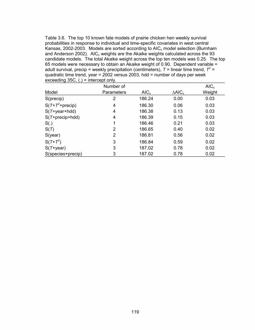
119

Table 3.6. The top 10 known fate models of prairie chicken hen weekly survival probabilities in response to individual and time-specific covariates in west central Kansas, 2002-2003. Models are sorted according to AICc model selection (Burnham and Anderson 2002). AICc weights are the Akaike weights calculated across the 93 candidate models. The total Akaike weight across the top ten models was 0.25. The top 65 models were necessary to obtain an Akaike weight of 0.90. Dependent variable = adult survival, precip = weekly precipitation (centimeters), T = linear time trend, T2 = quadratic time trend, year = 2002 versus 2003, hdd = number of days per week exceeding 35C, (.) = intercept only. Number of AICc Model Parameters AICc ∆AICc Weight S(precip) 2 186.24 0.00 0.03 S(T+T2+precip) 4 186.30 0.06 0.03 S(T+year+hdd) 4 186.38 0.13 0.03 S(T+precip+hdd) 4 186.39 0.15 0.03 S(.) 1 186.46 0.21 0.03 S(T) 2 186.65 0.40 0.02 S(year) 2 186.81 0.56 0.02 S(T+T2) 3 186.84 0.59 0.02 S(T+year) 3 187.02 0.78 0.02 S(species+precip) 3 187.02 0.78 0.02

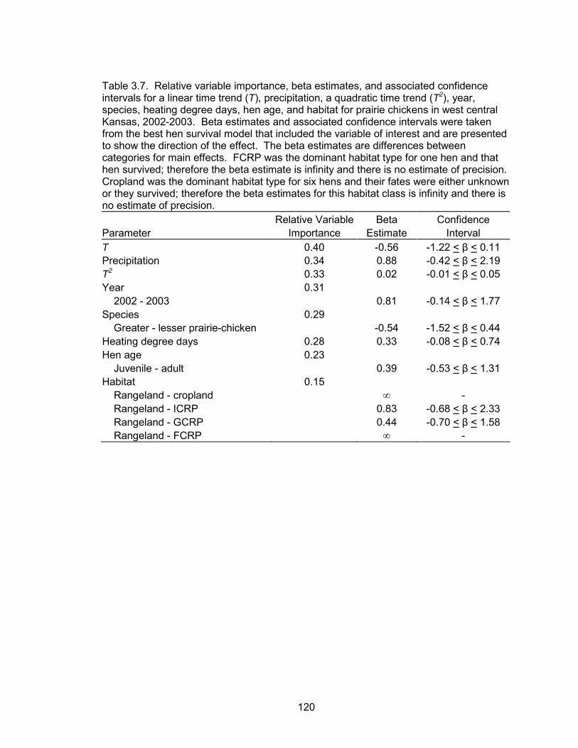
120

Table 3.7. Relative variable importance, beta estimates, and associated confidence intervals for a linear time trend (T), precipitation, a quadratic time trend (T2), year, species, heating degree days, hen age, and habitat for prairie chickens in west central Kansas, 2002-2003. Beta estimates and associated confidence intervals were taken from the best hen survival model that included the variable of interest and are presented to show the direction of the effect. The beta estimates are differences between categories for main effects. FCRP was the dominant habitat type for one hen and that hen survived; therefore the beta estimate is infinity and there is no estimate of precision. Cropland was the dominant habitat type for six hens and their fates were either unknown or they survived; therefore the beta estimates for this habitat class is infinity and there is no estimate of precision. Relative Variable Beta Confidence Parameter Importance Estimate Interval T 0.40 -0.56 -1.22 < β < 0.11 Precipitation 0.34 0.88 -0.42 < β < 2.19 T2 0.33 0.02 -0.01 < β < 0.05 Year 0.31 2002 - 2003 0.81 -0.14 < β < 1.77 Species 0.29 Greater - lesser prairie-chicken -0.54 -1.52 < β < 0.44 Heating degree days 0.28 0.33 -0.08 < β < 0.74 Hen age 0.23 Juvenile - adult 0.39 -0.53 < β < 1.31 Habitat 0.15 Rangeland - cropland ∞ - Rangeland - ICRP 0.83 -0.68 < β < 2.33 Rangeland - GCRP 0.44 -0.70 < β < 1.58 Rangeland - FCRP ∞ -

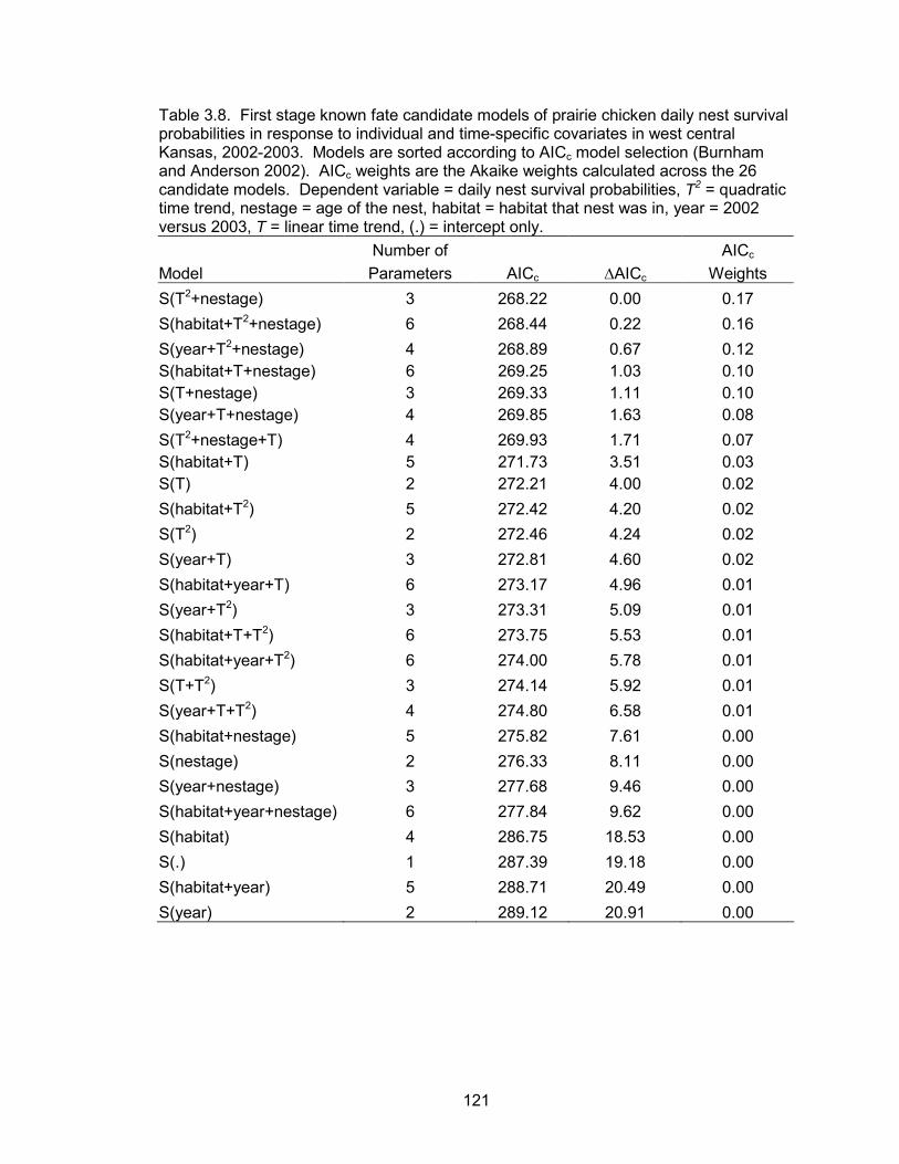
121

Table 3.8. First stage known fate candidate models of prairie chicken daily nest survival probabilities in response to individual and time-specific covariates in west central Kansas, 2002-2003. Models are sorted according to AICc model selection (Burnham and Anderson 2002). AICc weights are the Akaike weights calculated across the 26 candidate models. Dependent variable = daily nest survival probabilities, T2 = quadratic time trend, nestage = age of the nest, habitat = habitat that nest was in, year = 2002 versus 2003, T = linear time trend, (.) = intercept only. Number of AICc Model Parameters AICc ∆AICc Weights S(T2+nestage) 3 268.22 0.00 0.17 S(habitat+T2+nestage) 6 268.44 0.22 0.16 S(year+T2+nestage) 4 268.89 0.67 0.12 S(habitat+T+nestage) 6 269.25 1.03 0.10 S(T+nestage) 3 269.33 1.11 0.10 S(year+T+nestage) 4 269.85 1.63 0.08 S(T2+nestage+T) 4 269.93 1.71 0.07 S(habitat+T) 5 271.73 3.51 0.03 S(T) 2 272.21 4.00 0.02 S(habitat+T2) 5 272.42 4.20 0.02 S(T2) 2 272.46 4.24 0.02 S(year+T) 3 272.81 4.60 0.02 S(habitat+year+T) 6 273.17 4.96 0.01 S(year+T2) 3 273.31 5.09 0.01 S(habitat+T+T2) 6 273.75 5.53 0.01 S(habitat+year+T2) 6 274.00 5.78 0.01 S(T+T2) 3 274.14 5.92 0.01 S(year+T+T2) 4 274.80 6.58 0.01 S(habitat+nestage) 5 275.82 7.61 0.00 S(nestage) 2 276.33 8.11 0.00 S(year+nestage) 3 277.68 9.46 0.00 S(habitat+year+nestage) 6 277.84 9.62 0.00 S(habitat) 4 286.75 18.53 0.00 S(.) 1 287.39 19.18 0.00 S(habitat+year) 5 288.71 20.49 0.00 S(year) 2 289.12 20.91 0.00

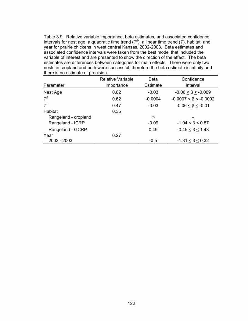
122

Table 3.9. Relative variable importance, beta estimates, and associated confidence intervals for nest age, a quadratic time trend (T2), a linear time trend (T), habitat, and year for prairie chickens in west central Kansas, 2002-2003. Beta estimates and associated confidence intervals were taken from the best model that included the variable of interest and are presented to show the direction of the effect. The beta estimates are differences between categories for main effects. There were only two nests in cropland and both were successful; therefore the beta estimate is infinity and there is no estimate of precision. Relative Variable Beta Confidence Parameter Importance Estimate Interval Nest Age 0.82 -0.03 -0.06 < β < -0.009 T2 0.62 -0.0004 -0.0007 < β < -0.0002 T 0.47 -0.03 -0.06 < β < -0.01 Habitat 0.35 Rangeland - cropland ∞ - Rangeland - ICRP -0.09 -1.04 < β < 0.87 Rangeland - GCRP 0.49 -0.45 < β < 1.43 Year 0.27 2002 - 2003 -0.5 -1.31 < β < 0.32

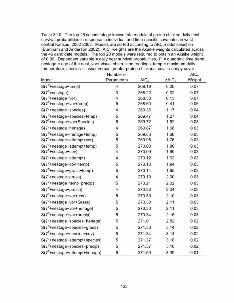
123

Table 3.10. The top 28 second stage known fate models of prairie chicken daily nest survival probabilities in response to individual and time-specific covariates in west central Kansas, 2002-2003. Models are sorted according to AICc model selection (Burnham and Anderson 2002). AICc weights are the Akaike weights calculated across the 46 candidate models. The top 28 models were required to obtain an Akaike weight of 0.90. Dependent variable = daily nest survival probabilities, T2 = quadratic time trend, nestage = age of the nest, vor= visual obstruction readings, temp = maximum daily temperature, species = lesser versus greater prairie-chickens, cov = canopy cover. Number of AICc Model Parameters AICc ∆AICc Weight S(T2+nestage+temp) 4 268.19 0.00 0.07 S(T2+nestage) 3 268.22 0.02 0.07 S(T2+nestage+vor) 4 268.33 0.13 0.07 S(T2+nestage+vor+temp) 5 268.60 0.41 0.06 S(T2+nestage+species) 4 269.36 1.17 0.04 S(T2+nestage+species+temp) 5 269.47 1.27 0.04 S(T2+nestage+vor+Species) 5 269.72 1.52 0.03 S(T2+nestage+henage) 4 269.87 1.68 0.03 S(T2+nestage+henage+temp) 5 269.88 1.68 0.03 S(T2+nestage+attempt+vor) 5 269.95 1.76 0.03 S(T2+nestage+attempt+temp) 5 270.00 1.80 0.03 S(T2+nestage+cov) 4 270.09 1.90 0.03 S(T2+nestage+attempt) 4 270.12 1.92 0.03 S(T2+nestage+cov+temp) 5 270.13 1.94 0.03 S(T2+nestage+grass+temp) 5 270.14 1.95 0.03 S(T2+nestage+grass) 4 270.19 2.00 0.03 S(T2+nestage+temp+precip) 5 270.21 2.02 0.03 S(T2+nestage+precip) 4 270.23 2.04 0.03 S(T2+nestage+vor+cov) 5 270.30 2.10 0.03 S(T2+nestage+vor+Grass) 5 270.30 2.11 0.03 S(T2+nestage+vor+henage) 5 270.30 2.11 0.03 S(T2+nestage+vor+precip) 5 270.34 2.15 0.03 S(T2+nestage+species+henage) 5 271.01 2.82 0.02 S(T2+nestage+species+grass) 5 271.33 3.14 0.02 S(T2+nestage+species+cov) 5 271.34 3.14 0.02 S(T2+nestage+attempt+species) 5 271.37 3.18 0.02 S(T2+nestage+species+precip) 5 271.37 3.18 0.02 S(T2+nestage+attempt+henage) 5 271.59 3.39 0.01

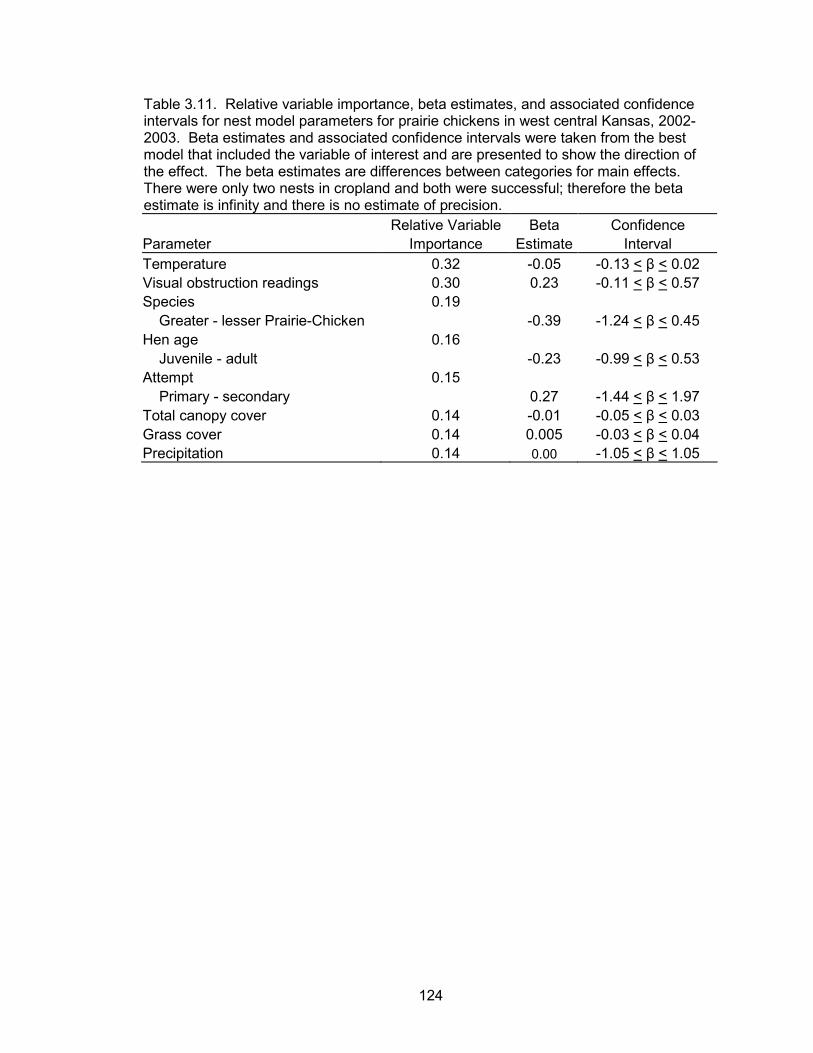
124

Table 3.11. Relative variable importance, beta estimates, and associated confidence intervals for nest model parameters for prairie chickens in west central Kansas, 2002-2003. Beta estimates and associated confidence intervals were taken from the best model that included the variable of interest and are presented to show the direction of the effect. The beta estimates are differences between categories for main effects. There were only two nests in cropland and both were successful; therefore the beta estimate is infinity and there is no estimate of precision. Relative Variable Beta Confidence Parameter Importance Estimate Interval Temperature 0.32 -0.05 -0.13 < β < 0.02 Visual obstruction readings 0.30 0.23 -0.11 < β < 0.57 Species 0.19 Greater - lesser Prairie-Chicken -0.39 -1.24 < β < 0.45 Hen age 0.16 Juvenile - adult -0.23 -0.99 < β < 0.53 Attempt 0.15 Primary - secondary 0.27 -1.44 < β < 1.97 Total canopy cover 0.14 -0.01 -0.05 < β < 0.03 Grass cover 0.14 0.005 -0.03 < β < 0.04 Precipitation 0.14 0.00 -1.05 < β < 1.05

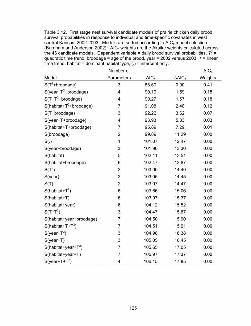
125

Table 3.12. First stage nest survival candidate models of prairie chicken daily brood survival probabilities in response to individual and time-specific covariates in west central Kansas, 2002-2003. Models are sorted according to AICc model selection (Burnham and Anderson 2002). AICc weights are the Akaike weights calculated across the 46 candidate models. Dependent variable = daily brood survival probabilities, T2 = quadratic time trend, broodage = age of the brood, year = 2002 versus 2003, T = linear time trend, habitat = dominant habitat type, (.) = intercept only. Number of AICc Model Parameters AICc ∆AICc Weights S(T2+broodage) 3 88.60 0.00 0.41 S(year+T2+broodage) 4 90.19 1.59 0.18 S(T+T2+broodage) 4 90.27 1.67 0.18 S(habitat+T2+broodage) 7 91.08 2.48 0.12 S(T+broodage) 3 92.22 3.62 0.07 S(year+T+broodage) 4 93.93 5.33 0.03 S(habitat+T+broodage) 7 95.89 7.29 0.01 S(broodage) 2 99.89 11.29 0.00 S(.) 1 101.07 12.47 0.00 S(year+broodage) 3 101.90 13.30 0.00 S(habitat) 5 102.11 13.51 0.00 S(habitat+broodage) 6 102.47 13.87 0.00 S(T2) 2 103.00 14.40 0.00 S(year) 2 103.05 14.45 0.00 S(T) 2 103.07 14.47 0.00 S(habitat+T2) 6 103.66 15.06 0.00 S(habitat+T) 6 103.97 15.37 0.00 S(habitat+year) 6 104.12 15.52 0.00 S(T+T2) 3 104.47 15.87 0.00 S(habitat+year+broodage) 7 104.50 15.90 0.00 S(habitat+T+T2) 7 104.51 15.91 0.00 S(year+T2) 3 104.98 16.38 0.00 S(year+T) 3 105.05 16.45 0.00 S(habitat+year+T2) 7 105.65 17.05 0.00 S(habitat+year+T) 7 105.97 17.37 0.00 S(year+T+T2) 4 106.45 17.85 0.00

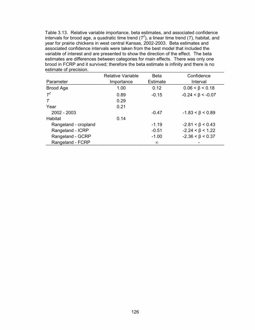
126

Table 3.13. Relative variable importance, beta estimates, and associated confidence intervals for brood age, a quadratic time trend (T2), a linear time trend (T), habitat, and year for prairie chickens in west central Kansas, 2002-2003. Beta estimates and associated confidence intervals were taken from the best model that included the variable of interest and are presented to show the direction of the effect. The beta estimates are differences between categories for main effects. There was only one brood in FCRP and it survived; therefore the beta estimate is infinity and there is no estimate of precision. Relative Variable Beta Confidence Parameter Importance Estimate Interval Brood Age 1.00 0.12 0.06 < β < 0.18 T2 0.89 -0.15 -0.24 < β < -0.07 T 0.29 Year 0.21 2002 - 2003 -0.47 -1.83 < β < 0.89 Habitat 0.14 Rangeland - cropland -1.19 -2.81 < β < 0.43 Rangeland - ICRP -0.51 -2.24 < β < 1.22 Rangeland - GCRP -1.00 -2.36 < β < 0.37 Rangeland - FCRP ∞ -

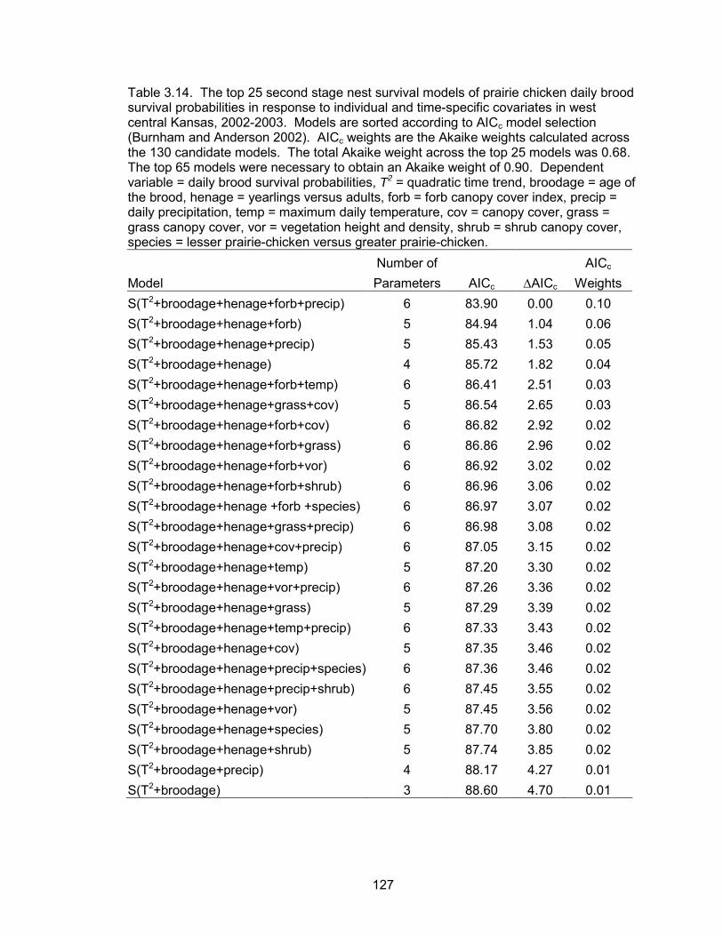
127

Table 3.14. The top 25 second stage nest survival models of prairie chicken daily brood survival probabilities in response to individual and time-specific covariates in west central Kansas, 2002-2003. Models are sorted according to AICc model selection (Burnham and Anderson 2002). AICc weights are the Akaike weights calculated across the 130 candidate models. The total Akaike weight across the top 25 models was 0.68. The top 65 models were necessary to obtain an Akaike weight of 0.90. Dependent variable = daily brood survival probabilities, T2 = quadratic time trend, broodage = age of the brood, henage = yearlings versus adults, forb = forb canopy cover index, precip = daily precipitation, temp = maximum daily temperature, cov = canopy cover, grass = grass canopy cover, vor = vegetation height and density, shrub = shrub canopy cover, species = lesser prairie-chicken versus greater prairie-chicken. Number of AICc Model Parameters AICc ∆AICc Weights S(T2+broodage+henage+forb+precip) 6 83.90 0.00 0.10 S(T2+broodage+henage+forb) 5 84.94 1.04 0.06 S(T2+broodage+henage+precip) 5 85.43 1.53 0.05 S(T2+broodage+henage) 4 85.72 1.82 0.04 S(T2+broodage+henage+forb+temp) 6 86.41 2.51 0.03 S(T2+broodage+henage+grass+cov) 5 86.54 2.65 0.03 S(T2+broodage+henage+forb+cov) 6 86.82 2.92 0.02 S(T2+broodage+henage+forb+grass) 6 86.86 2.96 0.02 S(T2+broodage+henage+forb+vor) 6 86.92 3.02 0.02 S(T2+broodage+henage+forb+shrub) 6 86.96 3.06 0.02 S(T2+broodage+henage +forb +species) 6 86.97 3.07 0.02 S(T2+broodage+henage+grass+precip) 6 86.98 3.08 0.02 S(T2+broodage+henage+cov+precip) 6 87.05 3.15 0.02 S(T2+broodage+henage+temp) 5 87.20 3.30 0.02 S(T2+broodage+henage+vor+precip) 6 87.26 3.36 0.02 S(T2+broodage+henage+grass) 5 87.29 3.39 0.02 S(T2+broodage+henage+temp+precip) 6 87.33 3.43 0.02 S(T2+broodage+henage+cov) 5 87.35 3.46 0.02 S(T2+broodage+henage+precip+species) 6 87.36 3.46 0.02 S(T2+broodage+henage+precip+shrub) 6 87.45 3.55 0.02 S(T2+broodage+henage+vor) 5 87.45 3.56 0.02 S(T2+broodage+henage+species) 5 87.70 3.80 0.02 S(T2+broodage+henage+shrub) 5 87.74 3.85 0.02 S(T2+broodage+precip) 4 88.17 4.27 0.01 S(T2+broodage) 3 88.60 4.70 0.01

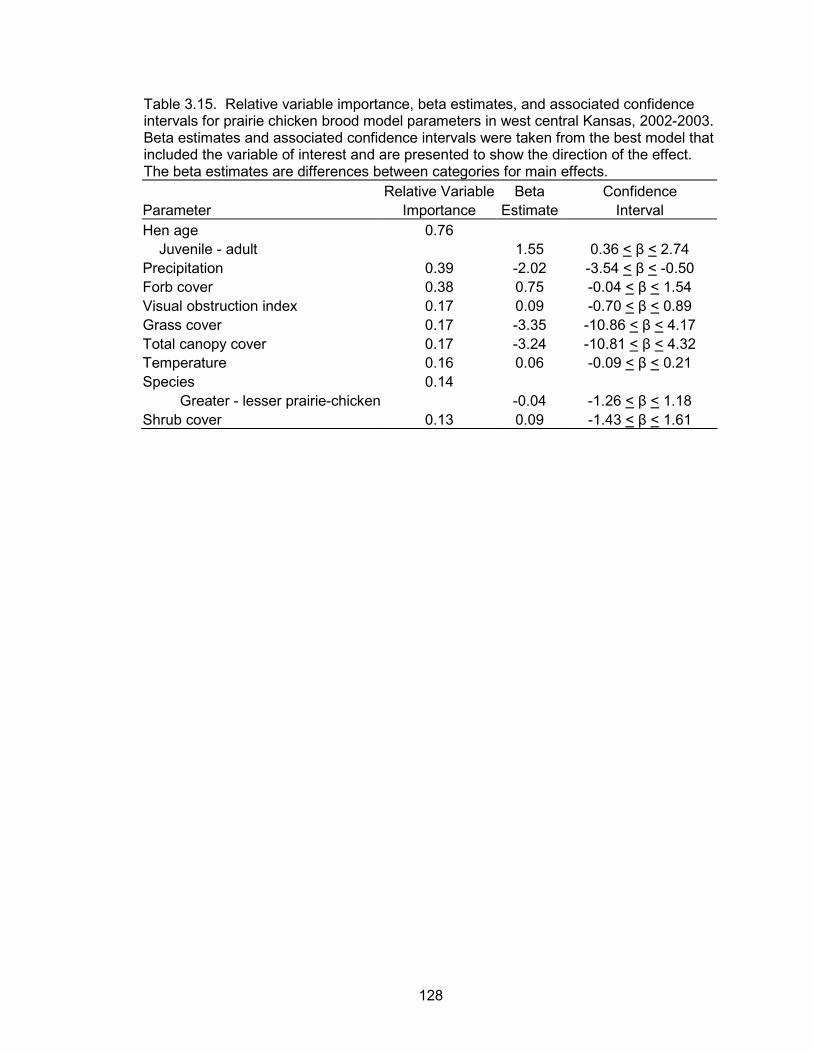
128

Table 3.15. Relative variable importance, beta estimates, and associated confidence intervals for prairie chicken brood model parameters in west central Kansas, 2002-2003. Beta estimates and associated confidence intervals were taken from the best model that included the variable of interest and are presented to show the direction of the effect. The beta estimates are differences between categories for main effects. Relative Variable Beta Confidence Parameter Importance Estimate Interval Hen age 0.76 Juvenile - adult 1.55 0.36 < β < 2.74 Precipitation 0.39 -2.02 -3.54 < β < -0.50 Forb cover 0.38 0.75 -0.04 < β < 1.54 Visual obstruction index 0.17 0.09 -0.70 < β < 0.89 Grass cover 0.17 -3.35 -10.86 < β < 4.17 Total canopy cover 0.17 -3.24 -10.81 < β < 4.32 Temperature 0.16 0.06 -0.09 < β < 0.21 Species 0.14

Greater - lesser prairie-chicken -0.04 -1.26 < β < 1.18 Shrub cover 0.13 0.09 -1.43 < β < 1.61

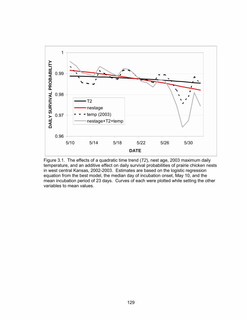
129

0.96

0.97

0.98

0.99

1

5/10 5/14 5/18 5/22 5/26 5/30

DATE

DA

ILY

SUR

VIVA

L PR

OB

AB

ILIT

Y

T2nestagetemp (2003)nestage+T2+temp

Figure 3.1. The effects of a quadratic time trend (T2), nest age, 2003 maximum daily temperature, and an additive effect on daily survival probabilities of prairie chicken nests in west central Kansas, 2002-2003. Estimates are based on the logistic regression equation from the best model, the median day of incubation onset, May 10, and the mean incubation period of 23 days. Curves of each were plotted while setting the other variables to mean values.

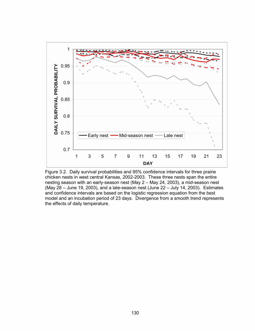
130

0.7

0.75

0.8

0.85

0.9

0.95

1

1 3 5 7 9 11 13 15 17 19 21 23DAY

DA

ILY

SUR

VIVA

L PR

OB

AB

ILIT

Y

Early nest Mid-season nest Late nest

Figure 3.2. Daily survival probabilities and 95% confidence intervals for three prairie chicken nests in west central Kansas, 2002-2003. These three nests span the entire nesting season with an early-season nest (May 2 � May 24, 2003), a mid-season nest (May 28 � June 19, 2003), and a late-season nest (June 22 � July 14, 2003). Estimates and confidence intervals are based on the logistic regression equation from the best model and an incubation period of 23 days. Divergence from a smooth trend represents the effects of daily temperature.

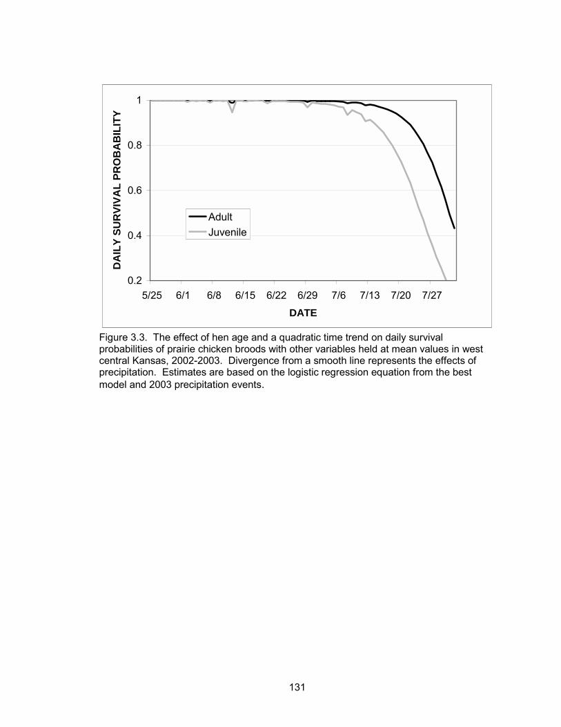
131

0.2

0.4

0.6

0.8

1

5/25 6/1 6/8 6/15 6/22 6/29 7/6 7/13 7/20 7/27

DATE

DA

ILY

SUR

VIVA

L PR

OB

AB

ILIT

Y

AdultJuvenile

Figure 3.3. The effect of hen age and a quadratic time trend on daily survival probabilities of prairie chicken broods with other variables held at mean values in west central Kansas, 2002-2003. Divergence from a smooth line represents the effects of precipitation. Estimates are based on the logistic regression equation from the best model and 2003 precipitation events.

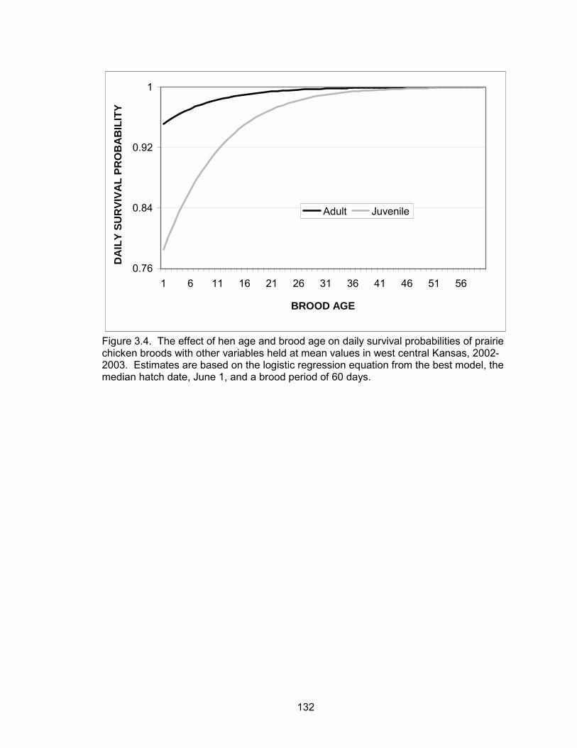
132

0.76

0.84

0.92

1

1 6 11 16 21 26 31 36 41 46 51 56

BROOD AGE

DA

ILY

SUR

VIVA

L PR

OB

AB

ILIT

Y

Adult Juvenile

Figure 3.4. The effect of hen age and brood age on daily survival probabilities of prairie chicken broods with other variables held at mean values in west central Kansas, 2002-2003. Estimates are based on the logistic regression equation from the best model, the median hatch date, June 1, and a brood period of 60 days.

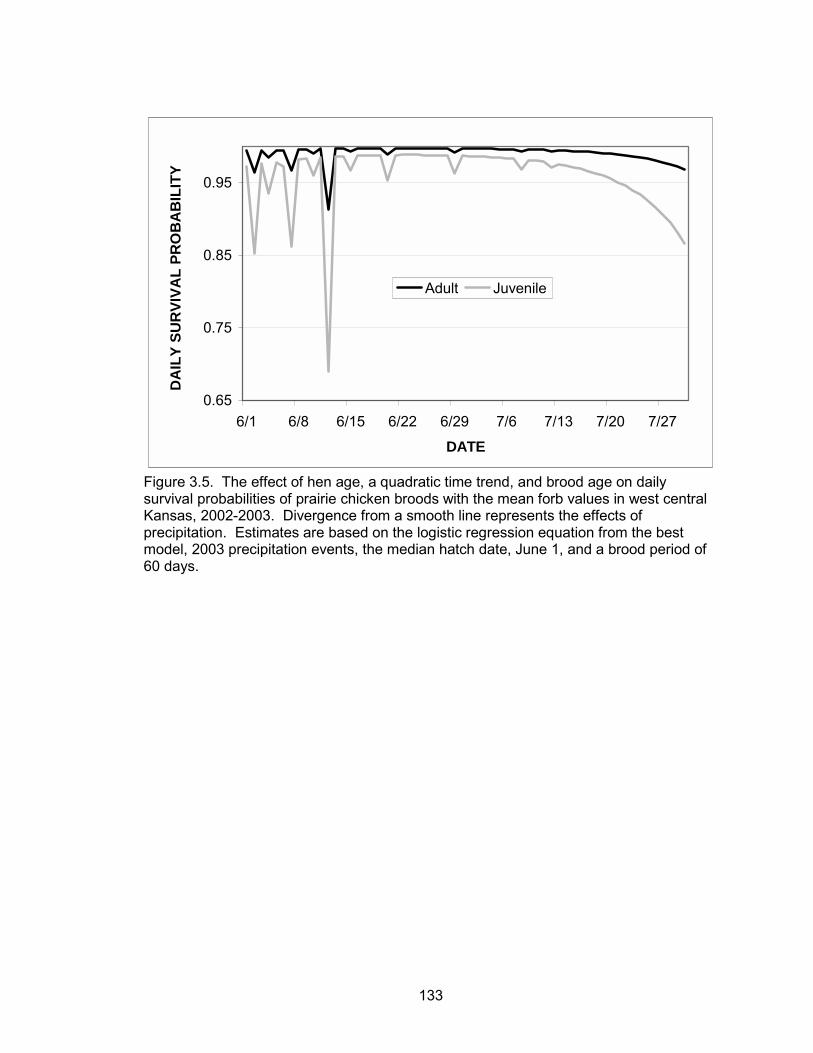
133

0.65

0.75

0.85

0.95

6/1 6/8 6/15 6/22 6/29 7/6 7/13 7/20 7/27

DATE

DA

ILY

SUR

VIVA

L PR

OB

AB

ILIT

Y

Adult Juvenile

Figure 3.5. The effect of hen age, a quadratic time trend, and brood age on daily survival probabilities of prairie chicken broods with the mean forb values in west central Kansas, 2002-2003. Divergence from a smooth line represents the effects of precipitation. Estimates are based on the logistic regression equation from the best model, 2003 precipitation events, the median hatch date, June 1, and a brood period of 60 days.

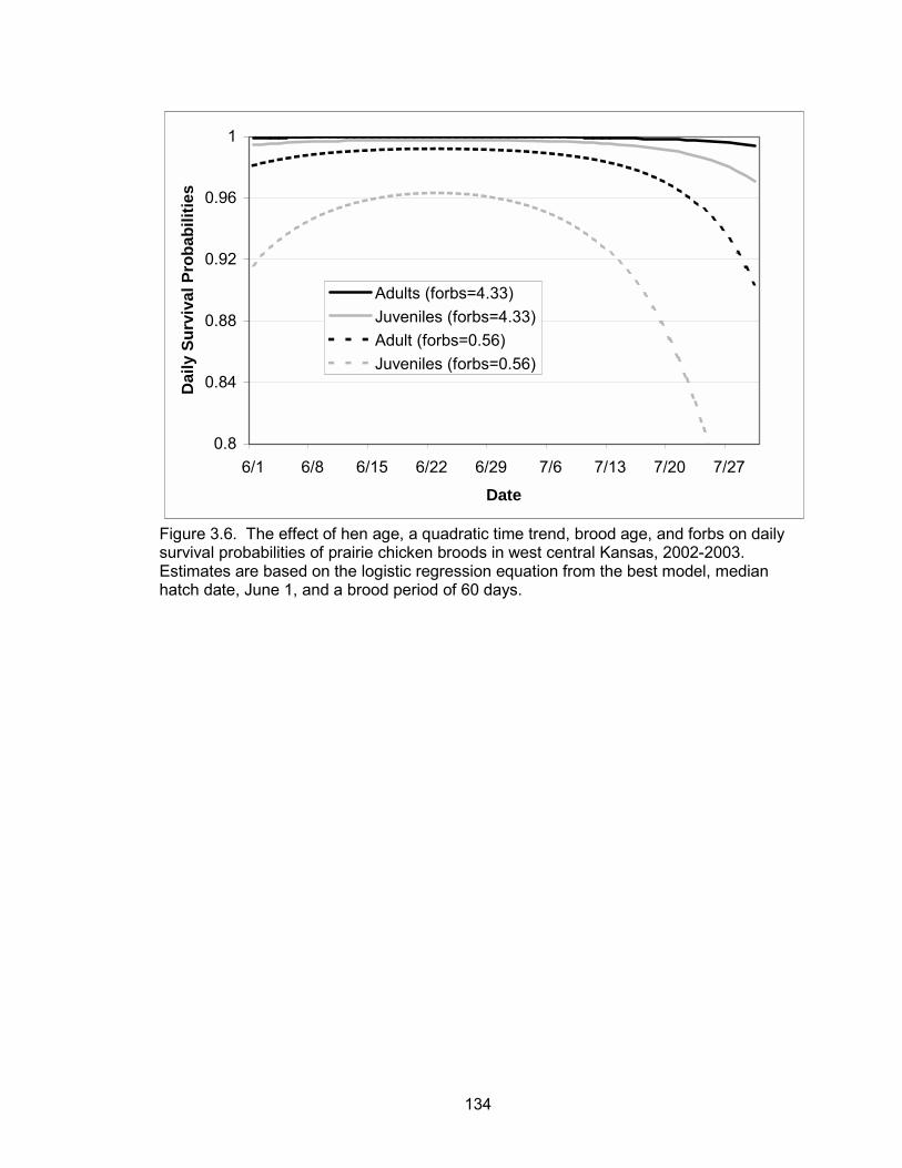
134

0.8

0.84

0.88

0.92

0.96

1

6/1 6/8 6/15 6/22 6/29 7/6 7/13 7/20 7/27

Date

Dai

ly S

urvi

val P

roba

bilit

ies

Adults (forbs=4.33)Juveniles (forbs=4.33)Adult (forbs=0.56)Juveniles (forbs=0.56)

Figure 3.6. The effect of hen age, a quadratic time trend, brood age, and forbs on daily survival probabilities of prairie chicken broods in west central Kansas, 2002-2003. Estimates are based on the logistic regression equation from the best model, median hatch date, June 1, and a brood period of 60 days.

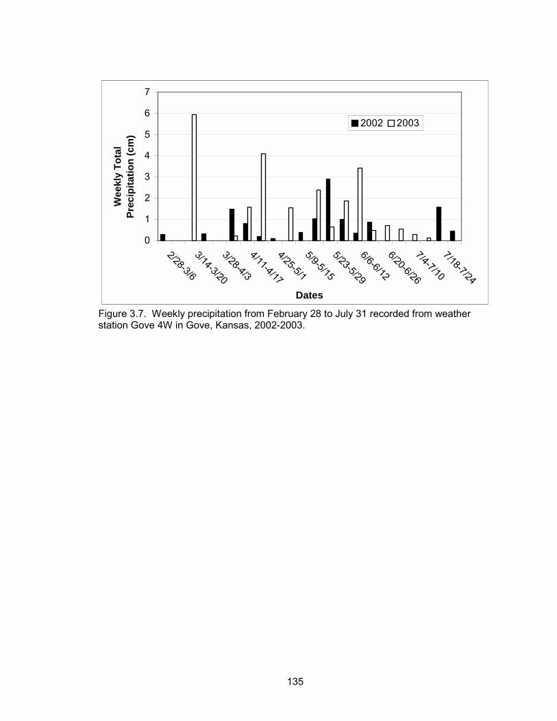
135

0

1

2

3

4

5

6

7

2/28-3/6

3/14-3/20

3/28-4/3

4/11-4/17

4/25-5/1

5/9-5/15

5/23-5/29

6/6-6/12

6/20-6/26

7/4-7/10

7/18-7/24

Dates

Wee

kly

Tota

l Pr

ecip

itatio

n (c

m)

2002 2003

Figure 3.7. Weekly precipitation from February 28 to July 31 recorded from weather station Gove 4W in Gove, Kansas, 2002-2003.

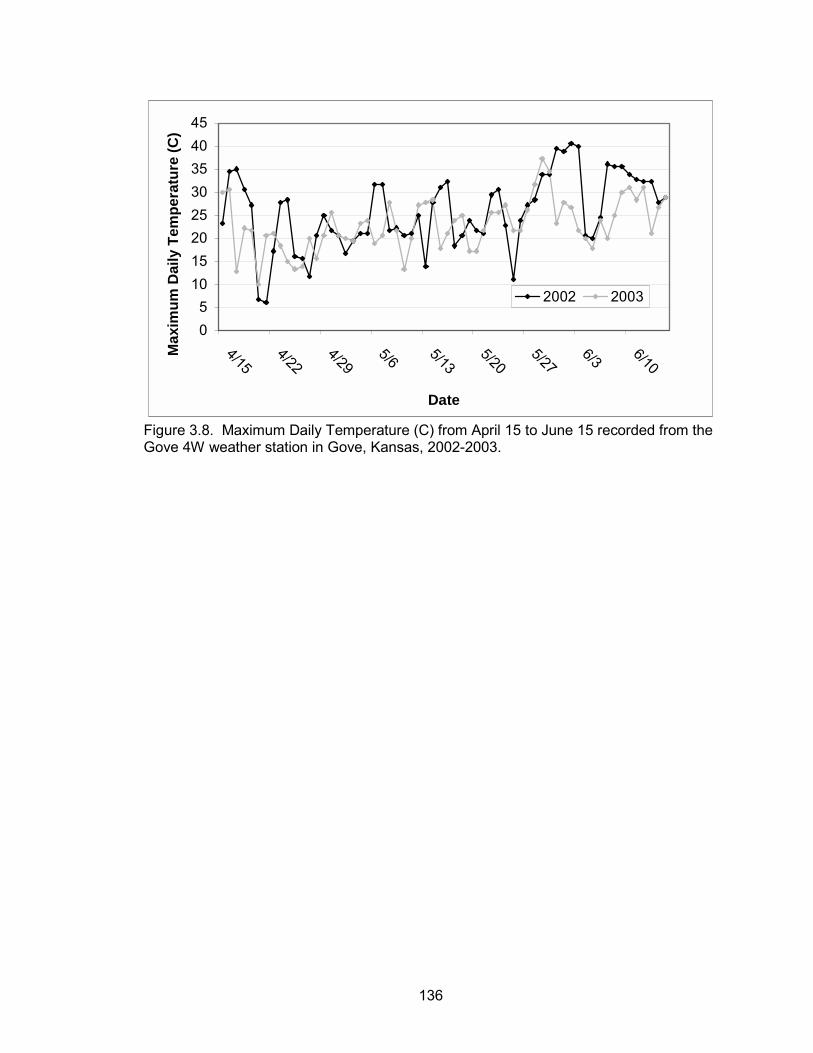
136

05

1015202530354045

4/154/22

4/295/6 5/13

5/205/27

6/3 6/10

Date

Max

imum

Dai

ly T

empe

ratu

re (C

)

2002 2003

Figure 3.8. Maximum Daily Temperature (C) from April 15 to June 15 recorded from the Gove 4W weather station in Gove, Kansas, 2002-2003.

thesis breeding season habitat use of conservation

Documents