thesis aquifer test methods to estimate …
TRANSCRIPT
THESIS
AQUIFER TEST METHODS TO ESTIMATE TRANSMISSIVITY AND WELL LOSS VIA A
SINGLE PUMPING WELL
Submitted by
James Anthony Roman
Department of Civil and Environmental Engineering
In partial fulfillment of the requirements
For the Degree of Master of Science
Colorado State University
Fort Collins, Colorado
Summer 2019
Master’s Committee:
Advisor: Tom C. Sale
Robert J. Sterrett
Michael J. Ronayne

ii
ABSTRACT
AQUIFER TEST METHODS TO ESTIMATE TRANSMISSIVITY AND WELL LOSS VIA A
SINGLE PUMPING WELL
Reducing the energy, environmental impacts, and costs required to produce groundwater from
wells is emerging as a critical concern in the modern world. Establishing and maintaining
pumping wells with minimal excess drawdown is thus important. Numerous methods have been
devised to quantify the aquifer and well contributions of the total drawdown in a pumping well.
The most common single-well methods involve step-drawdown test analyses that are inherently
subjective and cumbersome. The limitations are overcome here using simple, analytical methods
following the equations of Theis, Jacob, and Rorabaugh to estimate an aquifer’s transmissivity
and a well’s well-loss parameters and excess drawdown due to well-loss effects. The major steps
involve derivative analysis, solving systems of equations, and making elementary assumptions.
The proposed methods analyze data from independent constant-rate tests at single pumping
wells. In fact, Jacob’s well-loss coefficient of 4.6x10⁻⁷ day2m5 and 0.39𝑥10−7 day2m5 were estimated
at a pumping well via Jacob’s (1947) traditional step test analysis and the proposed method,
respectively. The reduced subjectivity of the proposed method suggests it produced the more
accurate estimate. The required energy and associated economic and environmental equivalences
of pumping the well loss are then calculated to suggest when further development of a new well
or the rehabilitation of a preexisting well is needed. The overall goal of this thesis is to advance
the proposed methods for more straightforward and objective analyses of aquifer test data in
academia and industry to promote the energy efficiency of groundwater production.

iii
ACKNOWLEDGMENTS
Field data was collected by Courtney Hemenway of Hemenway Groundwater Engineering.
Conceptual aide, presentation critiques, and encouragement were given from fellow students at
the Center of Contaminant Hydrology. Outstanding guidance and support were offered by my
advisor, Tom Sale, and committee, Bob Sterrett and Mike Ronayne. Funding for this study was
provided by the Chevron Corporation.
iv
TABLE OF CONTENTS
ABSTRACT .................................................................................................................................... ii
ACKNOWLEDGMENTS ............................................................................................................. iii
LIST OF TABLES ......................................................................................................................... vi
LIST OF FIGURES ...................................................................................................................... vii
1. INTRODUCTION .............................................................................................................. 1
1.1 Overview ............................................................................................................................. 1
1.2 Objectives ........................................................................................................................... 5
1.3 Organization ........................................................................................................................ 5
2. WORK BY OTHERS ......................................................................................................... 6
2.1 Definitions and Principal Equations ................................................................................... 6
2.1.1 Derivative Analysis .................................................................................................... 8
2.2 Well-Loss Contributors ....................................................................................................... 9
2.3 Limitations of Standard Single-Well Methods for Estimating Aquifer and Well Losses 11
3. METHODS ....................................................................................................................... 17
3.1 Estimating the Aquifer’s Transmissivity .......................................................................... 17
3.1.1 Via Derivative Analysis ........................................................................................... 17
3.1.2 Via Fitting a Trendline ............................................................................................. 19
3.2 Estimating Jacob’s Well-Loss Coefficient (𝑛 = 2) .......................................................... 20
3.3 Estimating Rorabaugh’s Well-Loss Coefficient and Well-Loss Exponent (2 ≤ 𝑛 ≤ 2.8)
................................................................................................................................................. 23
3.3.1 Optional 𝑛 Correction .............................................................................................. 26
3.4 Economic and Environmental Impacts of Pumping with Well Loss ................................ 28
4. APPLICATION ................................................................................................................ 31
4.1 Available Data .................................................................................................................. 31
4.1.1 Synthetic Data ......................................................................................................... 31
4.1.2 Field Data ................................................................................................................ 32
4.2 Aquifer Transmissivity Estimates ..................................................................................... 34
4.2.1 Via Derivative Analysis .......................................................................................... 34
4.2.2 Via Fitting a Trendline ............................................................................................ 37
4.3 Rorabaugh and Jacob’s Well-Loss Coefficient and Well-Loss Exponent ........................ 38
4.3.1 Rorabaugh’s Assumption (2 ≤ 𝑛 ≤ 2.8) ................................................................ 38
4.3.2 Standard Step-Drawdown Test Analysis of The Field Well Data .......................... 39
4.3.3 Jacob’s Assumption (𝑛 = 2) .................................................................................... 41
4.3.4 Economic and Environmental Impacts of Pumping with Well Loss ....................... 43
5. CONCLUSION ................................................................................................................. 45
5.1 Summary ........................................................................................................................... 45
5.2 Recommendations for Future Work.................................................................................. 46
REFERENCES ............................................................................................................................. 48

v
APPENDIX I ................................................................................................................................ 52
LIST OF ABBREVIATIONS ....................................................................................................... 53

vi
LIST OF TABLES
Table 1 – Synthetic Data Aquifer Parameters and Pumping Rates .............................................. 31
Table 2 – Predefined Well-Loss Parameters and Solution Results............................................... 38
Table 3 – Inputs and Results of Economic and Environmental Impact Analyses of the Field
Well's Subsequent 𝑠𝑤 (given 𝑛 = 2) ............................................................................................ 43
Table 4 – Walton’s (1962) Well Performance Criteria Based on Well-Loss Coefficient Estimates
....................................................................................................................................................... 52

vii
LIST OF FIGURES
Figure 1 – An example of the hydraulic heads that contribute to total dynamic head (TDH) of a
domestic groundwater well system ................................................................................................. 1
Figure 2 – Conceptual model of aquifer and well losses about a pumping well ............................ 3
Figure 3 – Well-loss effects on 𝑟𝑒2𝑆 estimates at a pumping well via Theis (1935) curve
matching ........................................................................................................................................ 13
Figure 4 – Well-loss effects on 𝑟𝑒2𝑆 estimates via the Cooper-Jacob (1946) straight-line method
....................................................................................................................................................... 14
Figure 5 – Exponential calculations of a pumping well with aquifer parameters representative of
a confined aquifer ......................................................................................................................... 18
Figure 6 – Conceptual plot of specific drawdown vs log 𝑡∗ ......................................................... 22
Figure 7 – Polynomial regression model for 𝑛𝑐𝑜𝑟𝑟𝑒𝑐𝑡𝑒𝑑 given the overpredicted 𝑛𝑚𝑜𝑑𝑒𝑙 ............ 27
Figure 8 – Step-drawdown and constant-rate drawdown curves with their best-fit equations from
a groundwater production well in Castle Rock, CO; 𝑄𝑠𝑡𝑒𝑝_1 = 2180 𝑚3/𝑑𝑎𝑦, 𝑄𝑐𝑜𝑛𝑠𝑡𝑎𝑛𝑡_2 =3820 𝑚3/𝑑𝑎𝑦 ............................................................................................................................... 33
Figure 9 – 𝑇(𝑡) estimates of the synthetic data using Equation 18 with 𝑄3 = 550 𝑚3/day ....... 34
Figure 10a – 𝑇(𝑡) estimates, the average, and 95% confidence interval of the field well’s constant-rate test using Equation 18 ............................................................................................. 36
Figure 10b – 𝛺 estimates, the average, and 95% confidence interval of the field well’s constant-rate test using Equation 19 ............................................................................................................ 36
Figure 11 – Jacob’s (1947) traditional methodology for the step-drawdown test’s 𝐶𝐽 ................. 40
Figure 12a - The field well’s s/Q vs 𝑡 plot ................................................................................... 41
Figure 12b – The field well’s 𝐶𝐽 vs 𝑡 plot ..................................................................................... 41

1
1. INTRODUCTION
1.1 Overview
Groundwater production for water supply, irrigation, and industry has been increasing with a
growing world population (Konikow 2015). Emerging concerns of expanding groundwater
production include the energy required to lift water out of aquifers and the associated economic
and environmental costs. For example, as much as one third of the total electrical power use and
carbon footprint for a house between Denver and Colorado Springs can be attributed to the
energy needed to lift water from the underlying Denver Basin Aquifers (Ronayne et al. 2017).
The principle factors that govern the energy needed to produce groundwater are total dynamic
head (TDH) and the efficiency of the mechanical equipment including pumps, motors, and motor
drives. A well system’s TDH [L] is the total head required to lift water out of the aquifer to a
point of use while meeting pressure needs and overcoming all head losses throughout the system.
As an example, the head components of a domestic groundwater well are illustrated in Figure 1.
Figure 1 – An example of the hydraulic heads that contribute to total dynamic head (TDH) of a domestic
groundwater well system
2
Correspondingly, TDH can be defined as:
𝑇𝐷𝐻 = ℎ𝑓 + ℎ𝑝 + ℎ𝑢𝑠𝑒 + 𝐷𝑇𝑊𝑠𝑡𝑎𝑡𝑖𝑐 + 𝑠𝑎𝑞 + 𝑠𝑤 (1)
where ℎ𝑓 [L] is the friction losses contributable to conveyance, ℎ𝑝 [L] is the pressure head
required for sufficient discharge at the point of use (i.e., the house’s top-floor faucet), ℎ𝑢𝑠𝑒 [L] is
the elevation change from the well head to the point of use, 𝐷𝑇𝑊𝑠𝑡𝑎𝑡𝑖𝑐 [L] is the depth from the
well head to the static groundwater level prior to pumping, 𝑠𝑎𝑞 [L] is the drawdown associated
with pumping water from the aquifer, and 𝑠𝑤 [L] is the excess drawdown (or “well loss”)
associated with nonlaminar flows through the well during pumping.
This thesis has two goals. The first is to develop straightforward methods to accurately estimate
the aquifer’s transmissivity about a single pumping well. The second is to advance simple and
less subjective methods for quantifying a pumping well’s 𝑠𝑤 to support efforts that reduce energy
usage and the carbon footprint associated with groundwater production. Specifically, minimizing 𝑠𝑤 contributions to the total drawdown (𝑠𝑡𝑜𝑡𝑎𝑙 [L]) within a pumping well will reduce the
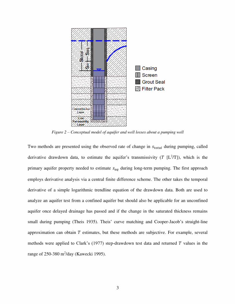
distance between the pumping water-level and the point of use. Figure 2 depicts a conceptual
model of the distribution of drawdowns about a pumping well.
3
Figure 2 – Conceptual model of aquifer and well losses about a pumping well
Two methods are presented using the observed rate of change in 𝑠𝑡𝑜𝑡𝑎𝑙 during pumping, called
derivative drawdown data, to estimate the aquifer’s transmissivity (𝑇 [L2/T]), which is the
primary aquifer property needed to estimate 𝑠𝑎𝑞 during long-term pumping. The first approach
employs derivative analysis via a central finite difference scheme. The other takes the temporal
derivative of a simple logarithmic trendline equation of the drawdown data. Both are used to
analyze an aquifer test from a confined aquifer but should also be applicable for an unconfined
aquifer once delayed drainage has passed and if the change in the saturated thickness remains
small during pumping (Theis 1935). Theis’ curve matching and Cooper-Jacob’s straight-line
approximation can obtain 𝑇 estimates, but these methods are subjective. For example, several
methods were applied to Clark’s (1977) step-drawdown test data and returned 𝑇 values in the
range of 250-380 m2/day (Kawecki 1995).

4
Next, two methodologies are advanced to quantify 𝑠𝑤 using drawdown data from a single
pumping well. The first methodology solves for Jacob’s well-loss coefficient (𝐶𝐽 [T2/L5]) while
the other resolves Rorabaugh’s well-loss coefficient (𝐶𝑅 [Tn/L3n-1]) then Rorabaugh’s well-loss
exponent (𝑛 [-]). Both methodologies utilize independent constant-rate aquifer tests. Finally, 𝑠𝑤
is resolved analytically and, thus, the proposed methods bypass the subjective nature of standard
step-drawdown test analyses initially advanced by Jacob (1947). The methods here are also
mathematically straightforward, so the complexity that is apparent with Rorabaugh’s (1953)
trial-and-error straight line approach and Sheahan’s (1971) family of type curves are overcome.
Moreover, the proposed methods can be considered economical as they do not require analyzing
data from observation wells, which can be expensive to design, install, and develop.
The proposed methods effectively bypass the subjective, complex, and cumbersome signatures
of standard single-well aquifer test analyses by building on the principal drawdown equations of
Theis (1935), Jacob (1946), and Rorabaugh (1953). The steps involved should be straightforward
enough for academia and industry to easily adopt the proposed methods in order to obtain more
accurate aquifer and well parameter estimates about a single pumping well. Economic and
environmental analyses are also conducted to ensure efficient well performance. Ultimately,
absolute 𝑠𝑤 values will prove useful for characterizing the efficacy of new groundwater well
installations and rehabilitation efforts of preexisting wells. For example, development of a new
well may be deemed sufficient if 𝑠𝑤 and the associated economic and environmental impacts of
pumping are low. Similarly, rehabilitation of a preexisting well will be suggested once the 𝑠𝑤
and associated economic and environmental effects become too large.
5
1.2 Objectives
The following work aims to develop straightforward methods to accurately estimate the aquifer’s
transmissivity, Jacob’s well-loss coefficient or Rorabaugh’s well-loss coefficient and well-loss
exponent, and subsequent excess drawdown (or “well loss”) due to nonlaminar flows at the
design pumping rate. The proposed methods highlight the efficacy of using well loss as a well
performance metric. Ultimately, the methods can quantify and ensure well loss in pumping wells
are minimized to reduce the energy and associated economic and environmental costs of
groundwater production.
1.3 Organization
The second section of this thesis introduces the principle drawdown equations including those of
Theis, Jacob, and Rorabaugh. Current method’s limitations and other background work are
reviewed to support the thesis’ subsequent efforts. The third section derives the aquifer and well
parameter solutions. The fourth section applies the proposed solutions to both field and synthetic
data to serve as a useful set of examples. The author also includes his interpretation and
recommendations to utilize the solutions effectively. The fifth section summarizes this thesis’
key results and implications while suggesting potential avenues for future efforts.

6
2. WORK BY OTHERS
This section presents the relevant knowledge of groundwater well hydraulics from the work of
others. Definitions and principal equations are established, factors that cause well loss are
reviewed, and the limitations of the existing aquifer test methods that estimate aquifer and well
parameters are discussed. This review provides a foundation for the subsequent Methods Section.
2.1 Definitions and Principal Equations
Equation 1 and Figure 2 illustrated that the 𝑠𝑡𝑜𝑡𝑎𝑙 at a pumping well can be simply defined as:
𝑠𝑡𝑜𝑡𝑎𝑙 = 𝑠𝑎𝑞 + 𝑠𝑤 (2)
Equation 2 is analogous to Jacob’s (1947) equation and is regarded as an integration of the
hydraulic losses throughout the flow field:
𝑠𝑡𝑜𝑡𝑎𝑙(𝑄, 𝑡) = 𝐵(𝑡)𝑄 + 𝐶𝐽𝑄2 (3)
where 𝐵(𝑡) is the aquifer-loss coefficient [T/L2] and 𝑄 is the well’s pumping rate [L3/T], thus 𝐵(𝑡)𝑄 is the “aquifer-loss term” [L] which actually accounts for all laminar flows in the aquifer-
well system (Kærgaard 1982; Kawecki 1995). Laminar flows typically occur in the formation,
skin zone, and gravel pack. Next, 𝐶𝐽 is Jacob’s well-loss coefficient [T2/L5], thus 𝐶𝐽𝑄2 is Jacob’s
“well-loss term” [L] that represents the head losses due to turbulent flows in the system.
Turbulent flow typically occurs through a well’s screens and inside the casing. Jacob assumed
the well-loss exponent, 𝑛 [-], is equal to 2 as the observed head loss for fully-developed turbulent
flow in a pipe is a function of 𝑄2 (Jacob 1947). As a result, Jacob’s equation does not account
for the non-linear laminar flow regime, which could describe flows through the formation

7
immediately about a well, the formation damaged by drilling fluids (skin zone), and/or gravel
pack (Houben 2015). Nonetheless, Jacob’s equation has been found to have a physical
background for reasonably homogenous regions about a well (Kærgaard 1982).
Rorabaugh’s (1953) equation for 𝑠𝑡𝑜𝑡𝑎𝑙, on the other hand, has an additional fitting parameter
that is used when Equation 3 is found to be inadequate to model a time series of drawdown data:
𝑠𝑡𝑜𝑡𝑎𝑙(𝑄, 𝑡) = 𝐵(𝑡)𝑄 + 𝐶𝑅𝑄𝑛 (4)
where 𝐶𝑅 is Rorabaugh’s well-loss coefficient [Tn/L3n-1], so 𝐶𝑅𝑄𝑛 is Rorabaugh’s “well-loss
term” [L]. Rorabaugh describes well-loss effects by leaving the well-loss exponent as an
unknown parameter to be estimated. The 𝑛 is reported to range between 2.4 and 2.8 with an
average of 2.5 for field data (Rorabaugh 1953). Some have referenced Lennox’s 1966 work to
infer that 𝑛 can even be as high as 3.5, but Lennox, two years later, stated that the data were
inadequate to put “too great a reliance on these results…some later test data which were
unavailable for the original paper have given values of [𝑛] less than 3” (Lennox 1968).
For both Equation 3 and 4, 𝐵(𝑡)𝑄 is time-dependent and can be represented by the Theis
equation for use in ideal confined aquifer settings or late-time, unconfined aquifer settings if the
change in the saturated thickness remains small during pumping (Theis 1935):
𝑠𝑎𝑞(𝑄, 𝑡) = 𝐵(𝑡)𝑄 = 𝑄4𝜋𝑇 ∫ 𝑒−𝑚𝑚 𝑑𝑚∞𝑢(𝑡)
𝑢(𝑡) = 𝑟2𝑆4𝑇𝑡
(5)
where 𝑇 is the aquifer’s transmissivity [L2/T], 𝑆 is the aquifer’s storage coefficient [-], 𝑟 is the
radial distance from the pumping well to a point of interest [L], 𝑡 is the elapsed time since

8
pumping began [T], and 𝑚 is the variable of integration. Since the proposed methods evaluate
the drawdown at the pumping well, the effective well radius (𝑟𝑒 [L]) can be substituted in for 𝑟 in
Equation 5 (Jacob 1947). The pumping well’s 𝑟𝑒 implicitly incorporates laminar well-loss effects
into 𝑠𝑎𝑞 (Kaecki 1995). Again, 𝑠𝑎𝑞 actually represents all laminar flows in the aquifer-well
system.
Comparing Equation 2 and 3 allows 𝑠𝑤, the excess drawdown during pumping (or “well loss”),
to be modeled as:
𝑠𝑤(𝑄) = 𝐶𝐽𝑄2 (6)
and, similarly, the likeness between Equations 2 and 4 allows for Rorabaugh’s 𝑠𝑤 model:
𝑠𝑤(𝑄) = 𝐶𝑅𝑄𝑛 (7)
An advantage of Jacob’s 𝑠𝑤 model (Equation 6) is that it only has one unknown parameter that
needs to be estimated. The advantage of Equation 7 is that the two unknown parameters can
provide the model more degrees of freedom to better fit the observed data.
2.1.1 Derivative Analysis
Following Lewis et al. (2016), 𝑠𝑤 effects at a pumping well can be removed via derivative
analysis. During a constant-rate test, 𝑄, 𝐶𝐽/𝐶𝑅, and 𝑛 are assumed to be constant, thus:
𝑑𝑠𝑤𝑑𝑡 = 0 (8)
which makes the temporal derivative of Equation 2 [𝑠𝑡𝑜𝑡𝑎𝑙 = 𝑠𝑎𝑞 + 𝑠𝑤]:
𝑑𝑠𝑡𝑜𝑡𝑎𝑙𝑑𝑡 = 𝑑𝑠𝑎𝑞𝑑𝑡 (9)
9
Similar to the solution obtained by Straface (2009), the derivative of Theis’ equation (Equation
5) with respect to time (via PTC Mathcad 2015) is:
𝑑𝑠𝑎𝑞𝑑𝑡 = 𝑄𝑒− 𝑟𝑒2𝑆4𝑇𝑡4𝜋𝑇𝑡 (10)
It is important to note that the improper integral of Theis’ equation was cleared since the
operations of differentiation and integration negate each other. Equation 10 can be simplified to
resolve transmissivity estimates from a single pumping well completed in a confined aquifer.
Section 3.1.1 develops this method further.
2.2 Well-Loss Contributors
Well-loss effects create nonlaminar flows that, in turn, cause 𝑠𝑤. Well-loss effects are
predominately dictated by the well’s design, drilling, and development (Clark 1977; Sterrett
2007; Hemenway 2018). Groundwater flow through a well’s screen and casing can also increase 𝑠𝑤, especially for deep wells with limited screen open-area (Clark 1977; Kawecki 1995; Sterrett
2007). Furthermore, other effects can cause the well loss to substantially increase over time
(Houben et al. 2018). The plethora of well-loss effects warrants a review of each, individual
contributor.
To start, the design of a groundwater production well plays a large role in governing 𝑠𝑤 during
pumping. As one example, open area is important for effective well development (Sterrett 2007).
Sufficient open area also ensures groundwater entrance velocities remain below 3 cm/s to
maintain laminar flow across the screens (Wendling et al. 1997; Sterrett 2007). If there is not
enough open area, then flow can become turbulent and cause well loss.

10
Secondly, drilling can significantly contribute to well loss in the case of near-well formation
damage. The degree of formation damage is highly dependent on the used drilling method. In the
case of high-capacity groundwater wells, the most common drilling method is mud rotary where
fluid pressure in a well is greater than the adjacent formation pressure (overbalanced drilling). As
a result, drilling fluid can be easily lost to the aquifer. The formation near the well is now
considered damaged with an area of reduced permeability, otherwise known as a “skin zone”.
Even wells drilled without drilling fluids can develop skin zones (Hanna et al. 2003; Sterrett
2007). Therefore, an objective of development procedures is to remove the skin zone, although it
is difficult to remove 100% of the drilling fluids. It is best practice to employ multiple
development techniques to enhance development efforts as much as possible (Sterrett 2007). If
development is insufficient, well loss will occur through the filter pack and skin zone.
Next, water flowing through a well’s casing is analogous to pipe flow. Thus, the head loss
through a well can be modeled with the Darcy-Weisbach equation, which is function of the “pipe
length” and square of the flow rate. In-casing well loss, therefore, become significant yet
unavoidable in deep wells (Carl 1977; Kawecki 1995) . Even keeping the casing velocity below
the recommended 1.5 m/s can still cause moderate friction losses in a well (Sterrett 2007).
Moreover, significant well loss can be contributed to the mechanical compaction of the filter
pack and clogging of the filter pack and well screens over time. This compaction and clogging
can reduce the filter pack’s porosity and screen open area, which would restrict flow paths and,
ultimately, cause well loss during pumping (Houben et al. 2018). Processes that induce clogging
can include the deposition of mineral phases (i.e., iron and manganese oxides and calcite), the
growth of biofilms, and the invasion of particles (Houben 2003; Houben and Treskatis 2007).

11
The aquifer’s transmissivity can quickly determine the relative importance of well-loss effects in
an aquifer-well system. Bierschenk (1963) explains that 𝑠𝑎𝑞 varies inversely with 𝑇. For
example, if 𝑇 is high, 𝑠𝑎𝑞 is small, therefore 𝑠𝑤 can be a relatively large proportion of 𝑠𝑡𝑜𝑡𝑎𝑙. Finally, a uniform distribution of inflow to a well seldom occurs in the field (Kærgaard 1982).
Given the log-normal distribution of hydraulic conductivity in nature, it follows the inflow could
be an order of magnitude greater than the mean. In other words, generally, 90% of the flow can
come from 10% of the aquifer section. Heterogeneity of the aquifer or skin layer can further
create preferential flow paths, ultimately affecting the vertical inflow distribution across a well’s
screen (Houben and Hauschild 2011). A similar effect can occur if a well screen has a poor
distribution of screen openings (either from improper well design or well screen clogging) that
causes excessive convergence flow near the individual openings (Sterrett 2007).
It quickly becomes apparent that there are many possible contributors of well loss in a pumping
well. Several of the contributors are interconnected and potentially synergistic, too. As such, the
proposed methodologies are important for quantifying 𝑠𝑤 at a well’s design pumping rate to
serve as a well performance metric. When 𝑠𝑤 estimates become too large, further development of
a new well or rehabilitation of a preexisting well should follow to ensure a community receives
and maintains an efficient groundwater well.
2.3 Limitations of Standard Single-Well Methods for Estimating Aquifer and Well Losses
There are several standard methods that strive to estimate the aquifer and well-loss contribution
of the total drawdown in a pumping well. Each method has limitations. The most common
methods and their limitations are discussed in further detail in this subsection.
12
The 𝑠𝑎𝑞 component of 𝑠𝑡𝑜𝑡𝑎𝑙 can be described with the aquifer’s properties. Currently, the
primary approaches to estimate the aquifer’s 𝑇 about a single pumping well analyze constant-rate
test data via Theis curve matching or the Cooper-Jacob straight line approximation (Fetter 2001;
Sterrett 2007; Mays 2012). Matching the curves or overlaying the line can be subjective and
subsequent results may vary significantly even between seasoned professionals.
The 𝑠𝑤 component of 𝑠𝑡𝑜𝑡𝑎𝑙 can be described with the well’s parameters. Typically, the
Rorabaugh (1953), Hantush-Bierschenk (1964), Sheahan (1971), and Eden-Hazel (1973)
techniques are used to resolve a well’s 𝐶 and 𝑛 (if not assumed to be 2). It is difficult to reliably
and consistently obtain each parameter, though, for many reasons.
To start, the four techniques all rely on step-drawdown test data. Step-drawdown test analyses
require a minimum of four, but ideally more, pumping steps for reliable estimates of 𝐶 (Jacob
1947; Rorabaugh 1953; Clark 1977; Singh 2002). Moreover, the measured drawdown after the
first step not only represents the pumping effects of itself, but also contains the residual
drawdown of the preceding steps (Kærgaard 1982). The data should be corrected for this effect if
it is analyzed, but that requires the aquifer’s 𝑇 and 𝑆. Also, drawdown estimates beyond the
second step may be incorrect due to erroneous extrapolation of drawdown trends (Lennox 1966;
Mogg 1969). As a result, step-drawdown test analyses can be highly subjective depending on
how a professional likes to procure and analyze step-drawdown test data.
The aforementioned techniques that resolve well parameters can be time-consuming (Jha et al.
2006; Memon et al. 2012). Kruseman and de Ridder (2000) show that the techniques involve
many steps, too, which create many opportunities to make mistakes. As a result, computer-based
approaches have been developed to analyze aquifer test data more quickly and consistently.
13
However, these approaches can be quite daunting, especially when the computer code is written
in an unfamiliar programming language or uses a complex mathematical operation.
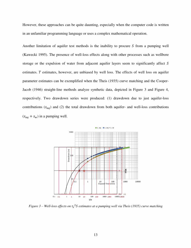
Another limitation of aquifer test methods is the inability to procure 𝑆 from a pumping well
(Kawecki 1995). The presence of well-loss effects along with other processes such as wellbore
storage or the expulsion of water from adjacent aquifer layers seem to significantly affect 𝑆
estimates. 𝑇 estimates, however, are unbiased by well loss. The effects of well loss on aquifer
parameter estimates can be exemplified when the Theis (1935) curve matching and the Cooper-
Jacob (1946) straight-line methods analyze synthetic data, depicted in Figure 3 and Figure 4,
respectively. Two drawdown series were produced: (1) drawdown due to just aquifer-loss
contributions (𝑠𝑎𝑞) and (2) the total drawdown from both aquifer- and well-loss contributions
(𝑠𝑎𝑞 + 𝑠𝑤) in a pumping well.
Figure 3 – Well-loss effects on 𝑟𝑒2𝑆 estimates at a pumping well via Theis (1935) curve matching

14
Theis’ ideal curve in Figure 3 is solely translated left towards a smaller 𝑡 when well-loss
contributions are added to the aquifer drawdown data, so the matched well function (𝑊(𝑢)) is
the same for each ideal curve. Thus, 𝑇 is unchanged between the 𝑠𝑎𝑞 and 𝑠𝑡𝑜𝑡𝑎𝑙 curves following
Theis’ equation for the aquifer’s transmissivity evaluated at a pumping well:
𝑇 = 𝑄4𝜋𝑠 W(𝑢) (11)
On the other hand, since the matched 𝑡 of 𝑠𝑡𝑜𝑡𝑎𝑙 is less than that of 𝑠𝑎𝑞, 𝑠𝑡𝑜𝑡𝑎𝑙’s 𝑟𝑒2𝑆 estimate
would be relatively smaller following Theis’ equation for the aquifer’s 𝑆 multiplied by 𝑟𝑒2:
𝑟𝑒2𝑆 = 4𝑇𝑡𝑢 (12)
Cooper-Jacob’s straight lines in Figure 4 further propound that well loss affects S estimates but
not 𝑇 estimates at a pumping well. Well loss translates the 𝑠𝑎𝑞 straight line upwards without
distorting its slope (∆𝑠 over the same log-cycle), so 𝑇 estimates are unchanged between the 𝑠𝑎𝑞
and 𝑠𝑡𝑜𝑡𝑎𝑙 lines following Cooper-Jacob’s equation for the aquifer’s transmissivity:
𝑇 = 2.3𝑄4𝜋∆𝑠 log (𝑡2𝑡1) (13)
Figure 4 – Well-loss effects on 𝑟𝑒2𝑆 estimates via the Cooper-Jacob (1946) straight-line method

15
The estimates of 𝑟𝑒2𝑆, however, are different between the two lines as the “𝑡 at zero-drawdown”, 𝑡𝑜 [L], has changed in Cooper-Jacob’s equation for the storage coefficient multiplied by 𝑟𝑒2:
𝑟𝑒2𝑆 = 2.25𝑇𝑡𝑜 (14)
The 𝑟𝑒2𝑆 estimate for 𝑠𝑡𝑜𝑡𝑎𝑙 would be smaller than that of 𝑠𝑎𝑞 since the 𝑠𝑡𝑜𝑡𝑎𝑙 line projects back
to a smaller 𝑡𝑜 compared to the 𝑠𝑎𝑞 line. Also, recall the data’s 𝑇 estimate was unchanged
between the two drawdown lines.
Consequently, 𝑆 cannot be calculated from pumping well drawdown data; perhaps if the total
well loss and effective well radius are both known precisely, but this is rarely the case (Clark
1977; Kawecki 1995). Some methods seek to estimate the fusion parameter 𝑟𝑒2𝑆, but this is not
of great use (Lennox 1966; Kawecki 1995). The aquifer’s 𝑇 and 𝑆 control groundwater flow, but 𝑇 is undoubtedly the predominant parameter for well yield at long-term pumping. As a result, 𝑆
will not be calculated here. The proposed methods are not dependent on 𝑆 values anyway.
Another major limitation of standard analyses is the use of well efficiency as a well performance
metric. Kawecki (1995) summarized the industry’s definition and caveats of well efficiency. Its
general form appears to be:
𝐸𝑤 = 𝑎𝑞𝑢𝑖𝑓𝑒𝑟 𝑙𝑜𝑠𝑠𝑎𝑞𝑢𝑖𝑓𝑒𝑟 𝑙𝑜𝑠𝑠 + 𝑤𝑒𝑙𝑙 𝑙𝑜𝑠𝑠 ∗ 100% (15)
The aquifer-loss and well-loss terms can be defined as they were for the total drawdown equation
to result in:
𝐸𝑤(𝑄, 𝑡) = 𝑠𝑎𝑞(𝑄, 𝑡)𝑠𝑎𝑞(𝑄, 𝑡) + 𝑠𝑤(𝑄) ∗ 100% (16)
16
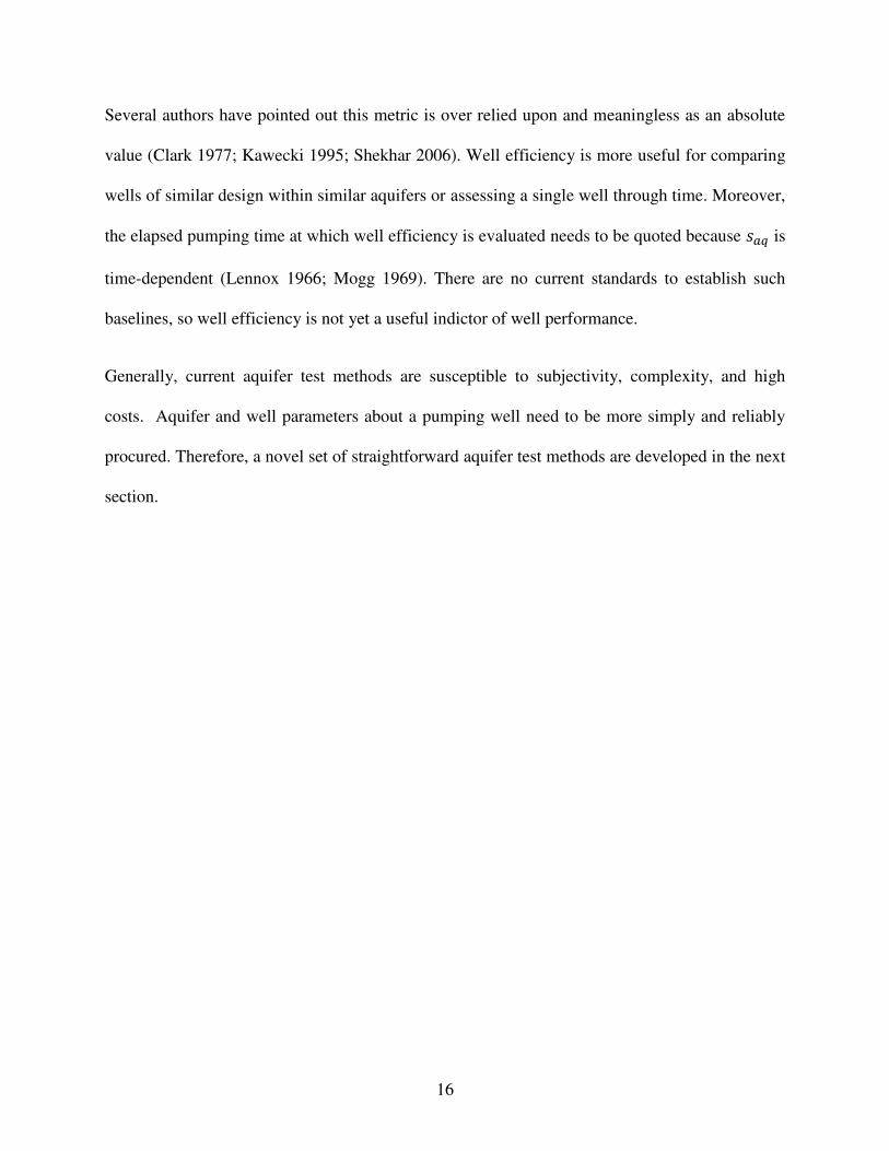
Several authors have pointed out this metric is over relied upon and meaningless as an absolute
value (Clark 1977; Kawecki 1995; Shekhar 2006). Well efficiency is more useful for comparing
wells of similar design within similar aquifers or assessing a single well through time. Moreover,
the elapsed pumping time at which well efficiency is evaluated needs to be quoted because 𝑠𝑎𝑞 is
time-dependent (Lennox 1966; Mogg 1969). There are no current standards to establish such
baselines, so well efficiency is not yet a useful indictor of well performance.
Generally, current aquifer test methods are susceptible to subjectivity, complexity, and high
costs. Aquifer and well parameters about a pumping well need to be more simply and reliably
procured. Therefore, a novel set of straightforward aquifer test methods are developed in the next
section.

17
3. METHODS
This section builds on the foundation laid by the previous Work by Others Section to develop
new methodologies to analyze aquifer test datasets. The proposed methods allow one to estimate
the aquifer’s transmissivity, Jacob’s well-loss coefficient, Rorabaugh’s well-loss coefficient and
well-loss exponent, and the economic and environmental equivalences of pumping well loss.
3.1 Estimating the Aquifer’s Transmissivity
3.1.1 Via Derivative Analysis
The aquifer’s transmissivity is the predominant parameter for anticipating the performance of
production wells. The aquifer’ storage coefficient is also important but hardly affects drawdowns
during long-term pumping. It is therefore imperative to resolve a reliable 𝑇 that is representative
of the aquifer system and, also, not biased by 𝑠𝑤. Following Lewis et al. (2016) and Equation 10, 𝑠𝑤 at a pumping well can be removed via derivative analysis.
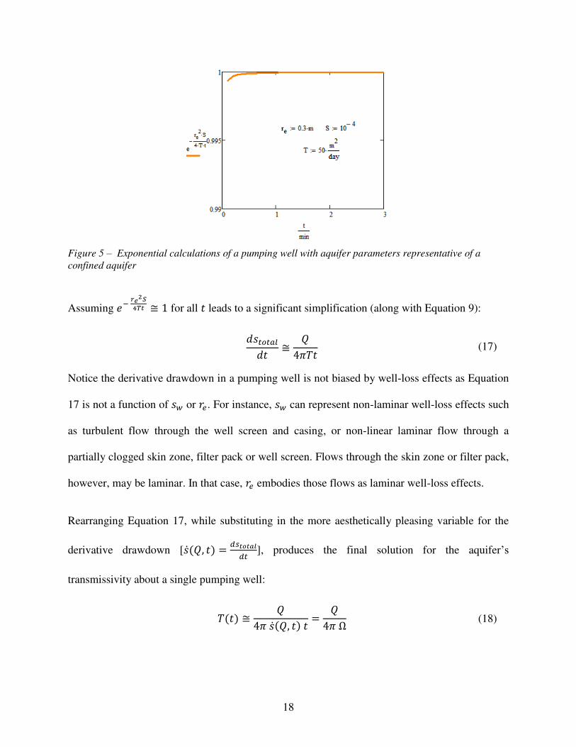
In fact, Equation 10 [𝑑𝑠𝑎𝑞𝑑𝑡 = 𝑄𝑒− 𝑟𝑒2𝑆4𝑇𝑡4𝜋𝑇𝑡 ] can be simplified to resolve transmissivity estimates from a
single pumping well. Since 𝑟𝑒 should be close to the radius of a pumping well, the 𝑟𝑒2𝑆4𝑇𝑡 argument
quickly becomes very small (i.e., less than 0.01). Then, 𝑒− 𝑟𝑒2𝑆4𝑇𝑡 will be very close to unity. An
example of the exponential calculations vs time at a pumping well with aquifer parameters
representative of a confined aquifer is shown in Figure 5.
18
Figure 5 – Exponential calculations of a pumping well with aquifer parameters representative of a
confined aquifer
Assuming 𝑒− 𝑟𝑒2𝑆4𝑇𝑡 ≅ 1 for all 𝑡 leads to a significant simplification (along with Equation 9):
𝑑𝑠𝑡𝑜𝑡𝑎𝑙𝑑𝑡 ≅ 𝑄4𝜋𝑇𝑡 (17)
Notice the derivative drawdown in a pumping well is not biased by well-loss effects as Equation
17 is not a function of 𝑠𝑤 or 𝑟𝑒. For instance, 𝑠𝑤 can represent non-laminar well-loss effects such
as turbulent flow through the well screen and casing, or non-linear laminar flow through a
partially clogged skin zone, filter pack or well screen. Flows through the skin zone or filter pack,
however, may be laminar. In that case, 𝑟𝑒 embodies those flows as laminar well-loss effects.
Rearranging Equation 17, while substituting in the more aesthetically pleasing variable for the
derivative drawdown [�̇�(𝑄, 𝑡) = 𝑑𝑠𝑡𝑜𝑡𝑎𝑙𝑑𝑡 ], produces the final solution for the aquifer’s
transmissivity about a single pumping well:
𝑇(𝑡) ≅ 𝑄4𝜋 �̇�(𝑄, 𝑡) 𝑡 = 𝑄4𝜋 Ω (18)

19
Generally, a confined aquifer’s 𝑇 should be constant through time about a given well location, so
the product of the two transient parameters in Equation 18 should result in a constant value for a
given 𝑄 and 𝑇:
�̇�(𝑄, 𝑡) 𝑡 = Ω = 𝑐𝑜𝑛𝑠𝑡𝑎𝑛𝑡 (19)
Therefore, Equation 18 can be plotted vs 𝑡 to arrive at the converging value. Otherwise, the
average value and a confidence interval of the 𝑇(𝑡) estimates should be calculated. For example,
the application of Equation 18 on field data produced oscillating 𝑇(𝑡) estimates about the
average value; Section 4.2.1 provides more details.
Notice the 𝑄 does not have to be the same between two different constant-rate tests to resolve the
same 𝑇 via Equation 18. When 𝑄 increases, the Ω [L] should correspondingly increase to
produce a consistent, final 𝑇 estimate at a well. More precisely, a larger pumping rate will impart
a greater stress on the aquifer, so a well’s derivative drawdown will proportionally increase to
resolve the same 𝑇 at a pumping well. Also notice estimates of the aquifer’s transmissivity will
be independent of nonlaminar well-loss effects as the 𝑠𝑤 term is not present in Equation 18.
3.1.2 Via Fitting a Trendline
Another quick, but non-analytical technique to procure 𝑇 can be done with a trendline. A time
series of drawdown data can be smoothed and fit with a natural logarithmic equation via the
scatter plot’s trendline function. Similarities between a logarithmic best-fit equation and Cooper-
Jacob’s (1946) approximation of 𝑠𝑎𝑞 allow the following steps:
𝑠𝑡𝑜𝑡𝑎𝑙(𝑄, 𝑡) = 𝑄4𝜋𝑇 ln (2.25𝑇𝑡𝑟𝑒2𝑆 ) + 𝑠𝑤(𝑄) (20a)

20
𝑠𝑡𝑜𝑡𝑎𝑙(𝑄, 𝑡) = 𝑄4𝜋𝑇 [ln(𝑡) + ln (2.25𝑇𝑟𝑒2𝑆 )] + 𝑠𝑤(𝑄) (20b)
𝑠𝑡𝑜𝑡𝑎𝑙(Q, 𝑡) = 𝑄4𝜋𝑇 ln(𝑡) + ( 𝑄4𝜋𝑇 ln (2.25𝑇𝑟𝑒2𝑆 ) + 𝑠𝑤(𝑄)) (20c)
𝑠𝑡𝑜𝑡𝑎𝑙(Q, 𝑡) = 𝜏1 ln(𝑡) + (𝜏2) (20d)
Equation 20d is a generalized form of Equation 20c and a logarithmic trendline equation using
condensed “best-fit equation parameters”, 𝜏1 and 𝜏2:
𝜏1 = 𝑄4𝜋𝑇 𝑎𝑛𝑑 𝜏2 = 𝑄4𝜋𝑇 ln (2.25𝑇𝑟𝑒2𝑆 ) + 𝑠𝑤(𝑄) (21)
Note that 𝜏1 = Ω since Ω = 𝑑𝑠𝑡𝑜𝑡𝑎𝑙𝑑𝑡 𝑡 = 𝑑𝑠𝑎𝑞𝑑𝑡 𝑡 = 𝑄4𝜋𝑇𝑡 𝑡 = 𝑄4𝜋𝑇 = 𝜏1.
Sequentially, the temporal derivative of Equation 20d is:
𝑑𝑠𝑡𝑜𝑡𝑎𝑙𝑑𝑡 = 𝜏1𝑡 (22)
which can be ultimately plugged into Equation 18 to quickly estimate 𝑇. Note that the derivative
solution is not biased by well-loss effects as the 𝑠𝑤 and 𝑟𝑒 parameters were removed.
3.2 Estimating Jacob’s Well-Loss Coefficient (𝒏 = 𝟐)
It should be reiterated that 𝑠𝑡𝑜𝑡𝑎𝑙 is the total drawdown due to contributions of head loss from
both the aquifer and the well. The exact effects of well loss in the field are not clearly
discernable, so there has been much debate on whether Jacob’s or Rorabaugh’s equation uses the
more appropriate 𝑠𝑤 definition. Jacob’s is supposedly more physically-based but many datasets
do not seem to fit his expression, so Rorabaugh presented a model that has an additional

21
parameter to better fit observed results. Thus, two methods for estimating well-loss parameters
are presented. The first method uses Jacob’s assumption that 𝑛 = 2. The second employs
Rorabaugh’s assumption that 𝑛 is an unknown parameter to be estimated, which will be resolved
in the next subsection.
To start, Equation 3, Jacob’s expression for 𝑠𝑡𝑜𝑡𝑎𝑙 at a pumping well, has only two unknown
parameters—𝐵(𝑡∗) and 𝐶𝐽. Thus, a simple system of two equations can be developed to solve for
the two unknowns. The two total drawdown equations are described via two independent
constant-rate tests ran at different pumping rates (𝑄1 and 𝑄2). Each constant-rate test is
considered “independent” as the water-level in the well returns to its original, static water-level
between the two pumping rates. The drawdown equations are then evaluated at the same time
after each aquifer test began, 𝑡∗, to make the equations directly comparable for subsequent
analysis. This can be summarized below while noting 𝑄1 < 𝑄2:
𝑠𝑡𝑜𝑡𝑎𝑙(𝑄1, 𝑡∗) = 𝐵(𝑡∗)𝑄1 + 𝐶𝐽𝑄12
𝑠𝑡𝑜𝑡𝑎𝑙(𝑄2, 𝑡∗) = 𝐵(𝑡∗)𝑄2 + 𝐶𝐽𝑄22
(23a)
(23b)
The two equations are then normalized by their respective 𝑄s (which produces specific
drawdown equations) and subtracted to eliminate one of the unknowns—𝐵(𝑡∗). Here, the
specific drawdown equation with the lower pumping rate is subtracted from that of the greater
pumping rate:
𝑠𝑡𝑜𝑡𝑎𝑙(𝑄2, 𝑡∗)𝑄2 − 𝑠𝑡𝑜𝑡𝑎𝑙(𝑄1, 𝑡∗)𝑄1 = 𝐶𝐽𝑄2 − 𝐶𝐽𝑄1 (24)
To simplify notation:

22
𝛥 (𝑠𝑡𝑜𝑡𝑎𝑙𝑄𝑖 )|2−1 = 𝑠𝑡𝑜𝑡𝑎𝑙(𝑄2, 𝑡∗)𝑄2 − 𝑠𝑡𝑜𝑡𝑎𝑙(𝑄1, 𝑡∗)𝑄1 (25)
Rearranging Equation 24 ultimately resolves the final solution for Jacob’s well-loss coefficient at
a pumping well assuming Jacob’s assumption that 𝑛 = 2:
𝐶𝐽 = 𝛥 (𝑠𝑡𝑜𝑡𝑎𝑙𝑄𝑖 )|2−1𝑄2 − 𝑄1 (26)
Equation 26 should be plotted vs 𝑡 to arrive at the converging value. It is important to realize that
the individual specific drawdowns vary in time, but their differences should quickly become
constant to result in a single 𝐶𝐽 for the analyzed pumping well. Lastly, 𝐶𝐽 can be used to
complete Jacob’s 𝑠𝑤(𝑄) = 𝐶𝐽𝑄2 model (Equation 6) to estimate the well loss in a pumping well.
Figure 6 is a conceptual plot of specific drawdowns vs log t∗. The offset between the lines is
indicative of well loss. For example, if there was no well loss (i.e., 𝐶𝐽 = 0) during pumping,
𝑠𝑡𝑜𝑡𝑎𝑙(𝑄1,𝑡∗)Q1 = B(t∗) = 𝑠𝑡𝑜𝑡𝑎𝑙(𝑄2,𝑡∗)Q2 , therefore the lines would lay on top of each other. Then, if well
loss increases, so would the offset between the two lines.
Figure 6 – Conceptual plot of specific drawdown vs log 𝑡∗
Since 𝐶𝐽 is now resolved, an expression for the other unknown in the system of equations can be
developed. Plugging Equation 26 into either drawdown expression (Equation 23a/b) produces:
23
𝐵(𝑡∗) = 𝑠𝑡𝑜𝑡𝑎𝑙(𝑄1, 𝑡∗) 𝑄22 − 𝑠𝑡𝑜𝑡𝑎𝑙(𝑄2, 𝑡∗) 𝑄12𝑄1 𝑄22 − 𝑄2 𝑄12 (27)
𝐵(𝑡∗), though, is not needed for the subsequent methods or analyses.
3.3 Estimating Rorabaugh’s Well-Loss Coefficient and Well-Loss Exponent (𝟐 ≤ 𝒏 ≤ 𝟐. 𝟖)
This method starts with Equation 4, Rorabaugh’s expression for 𝑠𝑡𝑜𝑡𝑎𝑙 at a pumping well. The
additional unknown parameter, 𝑛, makes the problem more complex. To resolve 𝐶𝑅 one must
first solve for 𝑛, but to solve for 𝑛 one must first make a critical assumption: the first, lowest
pumping rate, 𝑄1, is low enough to have 𝐶𝑅𝑄1𝑛 be essentially zero. In other words, 𝑄1 must be
small so basically no non-linear losses occur during pumping (𝑠𝑤 ≈ 0). This assumption relies
on the relative magnitude of the two head-loss coefficients in 𝑠𝑡𝑜𝑡𝑎𝑙. Because 𝐶𝑅 tends to be
significantly less than 𝐵(𝑡∗), as 𝑄 gets smaller the 𝑠𝑤 term will vanish much more quickly than
the 𝑠𝑎𝑞 term. A practical constant-rate to minimize well loss is assumed to be 10% of the pump’s
capacity (Hemenway 2018).
Similar to Equation 23, the observed drawdown is evaluated during two independent constant-
rate tests, but now 𝑄1 is assumed to be sufficiently low to neglect the non-linear well-loss term:
𝑠𝑡𝑜𝑡𝑎𝑙(𝑄1, 𝑡∗) = 𝐵(𝑡∗)𝑄1
𝑠𝑡𝑜𝑡𝑎𝑙(𝑄2, 𝑡∗) = 𝐵(𝑡∗)𝑄2 + 𝐶𝑅𝑄2𝑛
(28a)
(28b)
The two equations are normalized by their respective 𝑄 and subtracted to eliminate 𝐵(𝑡∗):
𝛥 (𝑠𝑡𝑜𝑡𝑎𝑙𝑄𝑖 )|2−1 = 𝐶𝑅 𝑄2𝑛−1 (29)

24
Equation 29 is then rearranged for an expression for the 𝐶𝑅 between the first and second
independent constant-rate tests:
𝐶𝑅 = 𝛥 (𝑠𝑡𝑜𝑡𝑎𝑙𝑄𝑖 )|2−1 𝑄2𝑛−1 (30)
Multiplying the right-hand side by 𝑄2𝑄2, Equation 30 is equivalent to:
𝐶𝑅 = 𝑄2 [𝛥 (𝑠𝑡𝑜𝑡𝑎𝑙𝑄𝑖 )|2−1] 𝑄2𝑛 (31)
Since Rorabaugh’s expression has three unknowns, a third equation must be introduced to
resolve 𝑛. The third equation is another 𝑠𝑡𝑜𝑡𝑎𝑙 expression during an even larger pumping rate, 𝑄3:
𝑠𝑡𝑜𝑡𝑎𝑙(𝑄3, 𝑡∗) = 𝐵(𝑡∗)𝑄3 + 𝐶𝑅𝑄3𝑛 (32)
Assuming 𝐶𝑅 is a constant between all specific drawdown curves, Equation 31 can be substituted
into Equation 32 with the simplifying notation:
𝑠𝑡𝑜𝑡𝑎𝑙(𝑄𝑖, 𝑡∗) = 𝑠𝑖(𝑡∗) where 𝑖 = 1, 2, 𝑜𝑟 3 (33)
and, since the first independent constant-rate test is assumed to experience no well loss:
𝑠1(𝑡∗)𝑄1 = 𝐵(𝑡∗) (34)
along with simplifying the numerator on the right-hand side of Equation 31 as:
𝑄2 [𝛥 (𝑠𝑡𝑜𝑡𝑎𝑙𝑄𝑖 )|2−1] = 𝑠2(𝑡∗) − 𝑄2𝑄1 𝑠1(𝑡∗) (35)
results in:

25
𝑠3(𝑡∗) = 𝑠1(𝑡∗)𝑄1 𝑄3 + [𝑠2(𝑡∗) − 𝑄2𝑄1 𝑠1(𝑡∗)] (𝑄3𝑄2)𝑛 (36)
Finally, rearranging Equation 36 resolves the expression for Rorabaugh’s 𝑛:
𝑛 = log (𝑠3(𝑡∗) − 𝑄3𝑄1 𝑠1(𝑡∗)𝑠2(𝑡∗) − 𝑄2𝑄1 𝑠1(𝑡∗))log (𝑄3𝑄2)⁄
(37)
Since 𝑛 is assumed to be a constant parameter, the two transient variables in the first log
operation’s numerator (𝑠1(𝑡∗) and 𝑠3(𝑡∗)) and denominator (𝑠1(𝑡∗) and 𝑠2(𝑡∗)) should change at
the same rate to result in constant differences. An estimate of 𝑛 via Equation 37 can now be
plugged into Equation 30/Equation 31 to estimate 𝐶𝑅. Together, the two well parameters can be
used to complete Rorabaugh’s 𝑠𝑤(𝑄) = 𝐶𝑅𝑄𝑛 model (Equation 7).
An 𝑠𝑤 value can also be estimated from Equation 25 [𝛥 (𝑠𝑡𝑜𝑡𝑎𝑙𝑄𝑖 )|2−1 = 𝑠𝑡𝑜𝑡𝑎𝑙(𝑄2,𝑡∗)𝑄2 − 𝑠𝑡𝑜𝑡𝑎𝑙(𝑄1,𝑡∗)𝑄1 ]
with Equation 2 [𝑠𝑡𝑜𝑡𝑎𝑙 = 𝑠𝑎𝑞 + 𝑠𝑤] substituted in while remembering 𝑠𝑤(𝑄1) ≈ 0:
𝛥 (𝑠𝑡𝑜𝑡𝑎𝑙𝑄𝑖 )|2−1 = 𝑠𝑎𝑞(𝑄2, 𝑡∗) + 𝑠𝑤(𝑄2)𝑄2 − 𝑠𝑎𝑞(𝑄1, 𝑡∗)𝑄1 (38)
Furthermore, substituting in a part of Equation 5 [𝑠𝑎𝑞(𝑄, 𝑡) = 𝐵(𝑡)𝑄] produces:
𝛥 (𝑠𝑡𝑜𝑡𝑎𝑙𝑄𝑖 )|2−1 = 𝐵(𝑡∗)𝑄2Q2 + 𝑠𝑤(𝑄2)𝑄2 − 𝐵(𝑡∗)𝑄1𝑄1 (39)
or:
𝛥 (𝑠𝑡𝑜𝑡𝑎𝑙𝑄𝑖 )|2−1 = 𝑠𝑤(𝑄2)𝑄2 (40)
26
Rearranging Equation 40 creates a direct expression for the absolute excess drawdown during the
second independent constant-rate test (if 𝑄1 is low enough to assume 𝑠𝑤(𝑄1) ≈ 0):
𝑠𝑤(𝑄2) = 𝑄2 [𝛥 (𝑠𝑡𝑜𝑡𝑎𝑙𝑄𝑖 )|2−1] (41)
Well loss calculations between the first and third independent constant-rate tests will have an
identical derivation. Therefore, Equation 41 can be generalized (and simplified) to an expression
for the excess drawdown during an independent constant-rate test with a pumping rate of 𝑄𝑖: 𝑠𝑤(𝑄𝑖) = 𝑠𝑖(𝑡∗) − 𝑄𝑖𝑄1 𝑠1(𝑡∗) (42)
As 𝑠𝑤(𝑄1) ≈ 0, the second term of Equation 42 is synonymous to 𝐵(𝑡∗)𝑄𝑖 but has the advantage
of not needing the well’s 𝑟𝑒 or aquifer’s 𝑆 to be resolved.
3.3.1 Optional 𝒏 Correction
The simplifying assumption that 𝑠𝑤 ≈ 0 for Rorabaugh’s 𝑠𝑡𝑜𝑡𝑎𝑙(𝑄1, 𝑡∗)— Equation 28a—instills
some error into well parameter estimates. It is not obvious, but 𝑛 will be overpredicted for all 𝑡
via Equation 37. The error should not be too great, especially as 𝑄1 becomes smaller. Still, a
polynomial regression model was made to correct 𝑛 back to some synthetic data’s 𝑛𝑝𝑟𝑒𝑑𝑒𝑓𝑖𝑛𝑒𝑑.
The synthetic drawdown data (of Rorabaugh’s 𝑠𝑡𝑜𝑡𝑎𝑙 expression for three independent constant-
rate tests) is introduced in further detail in Section 4.1.1.
Equation 37’s modeled 𝑛 (𝑛𝑚𝑜𝑑𝑒𝑙) is a function of the aquifer tests’ pumping rates. So, to create
the regression equation, the synthetic data was updated by iteratively changing two independent
variables—(1) 𝑛𝑝𝑟𝑒𝑑𝑒𝑓𝑖𝑛𝑒𝑑 and (2) 𝑄2%, 𝑄2’s percentage of 𝑄3— for the one dependent variable 𝑛𝑐𝑜𝑟𝑟𝑒𝑐𝑡𝑒𝑑. 𝑄1 was taken to be 10% of 𝑄3 due to practical constraints of the pump’s motor and

27
drive, but 𝑄2% was allowed to vary in case a project needs to test a particular pumping rate.
Changing the synthetic data’s predefined 𝐶𝑅, 𝑇, and 𝑆 had no effect on well parameter estimates.
Furthermore, the coefficients for 𝑄2% were found to be statistically insignificant at the 5% level,
so they were removed from the final solution for 𝑛𝑐𝑜𝑟𝑟𝑒𝑐𝑡𝑒𝑑:
𝑛𝑐𝑜𝑟𝑟𝑒𝑐𝑡𝑒𝑑 = −0.9304 + 1.576 𝑛𝑚𝑜𝑑𝑒𝑙 − 0.09141 𝑛𝑚𝑜𝑑𝑒𝑙2 (43)
The polynomial regression analysis is not consistent with the rest of the proposed methods’
theme of being analytical, but it is still simple as there is just one independent variable—𝑛𝑚𝑜𝑑𝑒𝑙. The analysis was completed via MATLAB® 2018b and is presented below in Figure 7.
Figure 7 – Polynomial regression model for 𝑛𝑐𝑜𝑟𝑟𝑒𝑐𝑡𝑒𝑑 given the overpredicted 𝑛𝑚𝑜𝑑𝑒𝑙 Notice the expression is dimensionless and has a R2 of 0.9998. Once 𝑛𝑐𝑜𝑟𝑟𝑒𝑐𝑡𝑒𝑑 is calculated, the
final, corrected solution for Rorabaugh’s well-loss coefficient at a pumping well is:
𝐶𝑅_𝑐𝑜𝑟𝑟𝑒𝑐𝑡𝑒𝑑 = 𝑠3(𝑡∗)𝑄3 − 𝑠2(𝑡∗)𝑄2𝑄3𝑛𝑐𝑜𝑟𝑟𝑒𝑐𝑡𝑒𝑑−1 − 𝑄2𝑛𝑐𝑜𝑟𝑟𝑒𝑐𝑡𝑒𝑑−1 (44)
Also note the value of 𝐵(𝑡∗) or any of the aquifer parameters were not required to resolve the
final 𝑛𝑐𝑜𝑟𝑟𝑒𝑐𝑡𝑒𝑑 or 𝐶𝑅_𝑐𝑜𝑟𝑟𝑒𝑐𝑡𝑒𝑑 estimates. Nonetheless, 𝐵(𝑡∗) can be estimated via Equation 34.
28
The author supports a modified set of aquifer tests—either (A) two independent constant-rate
tests with different pumping rates or (B) three independent constant-rate tests with different
pumping rates where one is sufficiently low for 𝑠𝑤(𝑄1) ≈ 0. Each independent constant-rate test
should last at least 60 minutes or, if real-time data are available, until drawdown measurements
appear to stabilize. The A set will produce data that can be used to estimate Jacob’s well-loss
coefficient. The B set will produce data so Rorabaugh’s well-loss coefficient and well-loss
exponent can be estimated. Depending on the set that was employed, a pumping well’s well loss
can be easily calculated via Jacob’s or Rorabaugh’s 𝑠𝑤 model. Through either method, the
subjectivity of standard step-drawdown test analyses can be avoided. Proposing a new type of
aquifer test may not seem the most appealing to practice, but an independent constant-rate test is
not that atypical.
3.4 Economic and Environmental Impacts of Pumping with Well Loss
Well loss increases the energy required to lift water out of the aquifer, causing a pumping’s
economic costs and environmental emissions to concurrently grow. The economic and
environmental impacts of well loss are important for highlighting the effects of nonlaminar flows
in a pumping well. Correspondingly, discussions of a groundwater well’s life-cycle assessment
(LCA) can be taken further, especially for the LCA’s “impact assessment” of a well’s “use
phase” (aka its operation).
The additionally required energy to pump the excess drawdown, 𝐸𝑝𝑢𝑚𝑝 [M L2/T2], is given by:
𝐸𝑝𝑢𝑚𝑝 = 𝑄𝜌𝑔𝑠𝑤𝑡𝑄𝜀 (45)
29
where 𝜌 [M/L3] is the density of the groundwater; 𝑔 [L/T2] is the acceleration due to gravity,
which the pump mostly needs to work against to deliver water vertically from the subsurface; 𝑡𝑄
is the duration of pumping; and 𝜀 [-] is the combined pump-motor-drive efficiency.
The economic impact (or “cost”) of the extra energy required to pump the well loss, 𝐸𝑐𝑜𝑠𝑡
[currency], can be sequentially developed via the cost rate of energy, 𝑅𝑐𝑜𝑠𝑡 [currency/(M L2/T2)]:
𝐸𝑐𝑜𝑠𝑡 = 𝑄𝜌𝑔𝑠𝑤𝑡𝑄𝜀 ∗ 𝑅𝑐𝑜𝑠𝑡 (46)
Similarly, the environmental impact (or “emissions”) of using the extra energy required to pump
the excess drawdown, 𝐸𝑒𝑛𝑣𝑖𝑟𝑜 [M], can be calculated with:
𝐸𝑒𝑛𝑣𝑖𝑟𝑜 = 𝑄𝜌𝑔𝑠𝑤𝜀 ∗ 𝑅𝑒𝑚𝑖𝑠𝑠𝑖𝑜𝑛 (47)
where 𝑅𝑒𝑚𝑖𝑠𝑠𝑖𝑜𝑛 [M/(M L2/T2)] is the mass emission rate of energy use. The emission rate seems
to vary depending on the energy source and efficiencies of producing the electricity for pumping.
Economic analysis can also determine when to rehabilitate a pumping well to ensure efficient
well performance. Rehabilitation is suggested when 𝐸𝑐𝑜𝑠𝑡 begins to outweigh the cost of
rehabilitation (𝑅𝑟𝑒ℎ𝑎𝑏 [currency]). This occurs once the two costs first equate, then exacerbates
when the 𝐸𝑐𝑜𝑠𝑡 increases due to a growing 𝑠𝑤 or larger 𝑡𝑄 of interest. The 𝑡𝑄 of interest depends
on the planning and management of the groundwater well. Regardless, the equivalent pumping
duration in which the cost of rehabilitation can provide (𝑡𝑄∗ [T]) is:
𝑡𝑄∗ = 𝜀 ∗ 𝑅𝑟𝑒ℎ𝑎𝑏𝑄𝜌𝑔𝑠𝑤 ∗ 𝑅𝑐𝑜𝑠𝑡 (48)

30
The other parameters in Equation 48 are assumed to remain constant; so, if pumping is desired
passed the calculated 𝑡𝑄∗ , then rehabilitation is advised. This can be mathematically stated as:
𝑡𝑄 ≥ 𝑡𝑄∗ (49)
In other words, if a well’s 𝑡𝑄 of interest is equal to or greater than the above 𝑡𝑄∗ , then it is time to
rehabilitate the pumping well. The 𝑡𝑄∗ equation conceptually makes sense according to the direct
and inverse proportionalities of Equation 48. For example, as the 𝑅𝑟𝑒ℎ𝑎𝑏 increases, so does 𝑡𝑄∗ .
Likewise, as the well’s 𝑄 increases, 𝑡𝑄∗ decreases.
31
4. APPLICATION
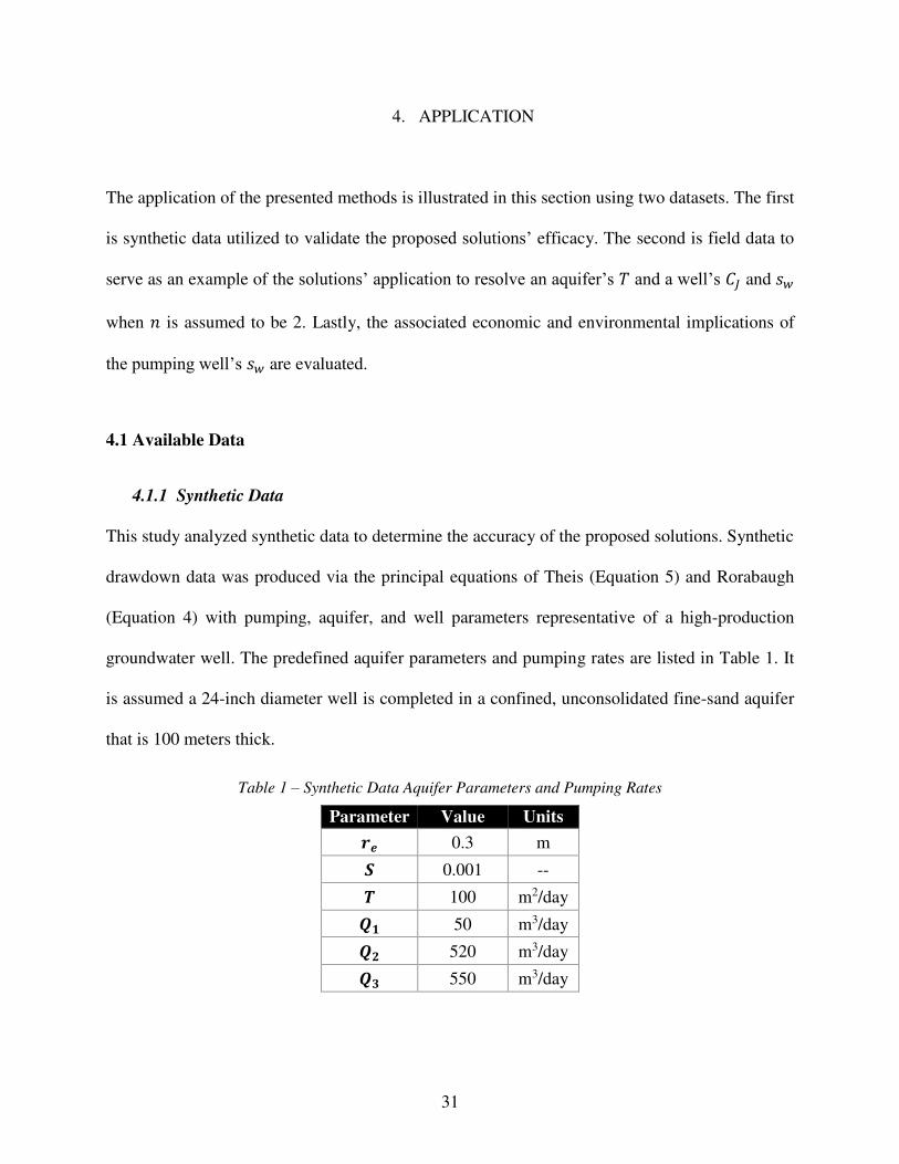
The application of the presented methods is illustrated in this section using two datasets. The first
is synthetic data utilized to validate the proposed solutions’ efficacy. The second is field data to
serve as an example of the solutions’ application to resolve an aquifer’s 𝑇 and a well’s 𝐶𝐽 and 𝑠𝑤
when 𝑛 is assumed to be 2. Lastly, the associated economic and environmental implications of
the pumping well’s 𝑠𝑤 are evaluated.
4.1 Available Data
4.1.1 Synthetic Data
This study analyzed synthetic data to determine the accuracy of the proposed solutions. Synthetic
drawdown data was produced via the principal equations of Theis (Equation 5) and Rorabaugh
(Equation 4) with pumping, aquifer, and well parameters representative of a high-production
groundwater well. The predefined aquifer parameters and pumping rates are listed in Table 1. It
is assumed a 24-inch diameter well is completed in a confined, unconsolidated fine-sand aquifer
that is 100 meters thick.
Table 1 – Synthetic Data Aquifer Parameters and Pumping Rates
Parameter Value Units 𝒓𝒆 0.3 m 𝑺 0.001 -- 𝑻 100 m2/day 𝑸𝟏 50 m3/day 𝑸𝟐 520 m3/day 𝑸𝟑 550 m3/day

32
Note, 𝑄3 (the third, largest pumping rate of the three independent constant-rate aquifer tests) was
set so 𝑠𝑡𝑜𝑡𝑎𝑙 would not exceed 8 meters after 60 minutes of pumping. It was found that setting 𝑄2
closer to 𝑄3 made 𝑛 results more accurate, as well—the nonlinearity of Equation 37 makes it
difficult to determine the reason. Therefore, 𝑄2 was assigned to be 95% of 𝑄3 as the smallest
pumping rate difference (∆𝑄) is assumed to be ~5% by which a variable frequency drive
submersible pump can be changed. Lastly, in order to make the 𝑠𝑤(𝑄1) ≈ 0 assumption valid, 𝑄1 was set to 10% of 𝑄3 as this is probably the lowest pumping rate (𝑄𝑚𝑖𝑛 = 10% ∗ 𝑄𝑚𝑎𝑥) that
the same pump can reliably maintain.
As for the predefined well parameters, 𝐶𝐽 = 1.5𝑥10−6 𝑑𝑎𝑦2𝑚5 when 𝑛 = 2 to depict a severely
clogged well (Walton 1962). Appendix I provides a table of Walton’s (1962) criteria of well
performance to serve as an easy reference for subsequent analyses. The predefined 𝐶𝑅 and 𝑛
values are provided within Table 2 in Section 4.3.1 when 𝑛 is allowed to vary.
4.1.2 Field Data
A 72-hour constant-rate aquifer test and a step-drawdown test dataset was collected from a newly
installed groundwater production well in the Denver Basin in Colorado by Hemenway
Groundwater Engineering. The “field well” taps into the Arapahoe aquifer which is a confined
sandstone aquifer with interbedding soft shale layers. The field well was completed with a 12-
inch diameter stainless steel v-slot wire wrap screens placed adjacent to the sandstone beds. The
field well was drilled via reverse circulation mud rotary then rigorously developed to maintain
the hydraulic connection to the aquifer. The field well is equipped with a variable frequency
drive submersible pump to ensure constant flowrates during pumping (Hemenway 2018). Figure
2 is a conceptual model for the pumping well and surrounding geology.

33
The utilized field data consists of high frequency (every two minutes) water level measurements
captured via a pressure transducer. Only some of the data was needed for the proposed
methods—the first step of a traditional step-drawdown test that lasted 60 minutes (with 𝑄1 =2180 𝑚3𝑑𝑎𝑦) and the first 60 minutes of the constant-rate test (with 𝑄2 = 3820 𝑚3𝑑𝑎𝑦). The water-
level in the well returned to its original, static position between the two tests, so they can be
considered “independent constant-rate tests”. The duration of these independent constant-rate
tests was short enough that the effects of water-level trends and barometric pressure changes on
drawdown data were neglected (Istok and Dawson 1991). All data was smoothed via a running
weighted mean, aka hanning. A logarithmic equation was then fit to the smoothed data to create
an even smoother drawdown curve. This was completed in Microsoft® Excel via the scatter
plot’s trendline function as illustrated in Figure 8. Note the very early data (𝑡 < 10𝑚𝑖𝑛) was not
included as it showed irregular behavior—probably due to well storage.
Figure 8 – Step-drawdown and constant-rate drawdown curves with their best-fit equations from a
groundwater production well in Castle Rock, CO; 𝑄𝑠𝑡𝑒𝑝_1 = 2180 𝑚3/𝑑𝑎𝑦, 𝑄𝑐𝑜𝑛𝑠𝑡𝑎𝑛𝑡_2 = 3820 𝑚3/𝑑𝑎𝑦
34
4.2 Aquifer Transmissivity Estimates
4.2.1 Via Derivative Analysis
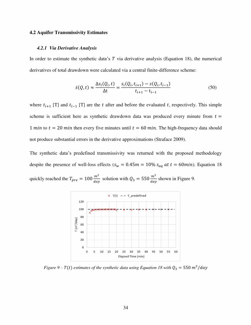
In order to estimate the synthetic data’s 𝑇 via derivative analysis (Equation 18), the numerical
derivatives of total drawdown were calculated via a central finite-difference scheme:
�̇�(𝑄, 𝑡) ≈ ∆𝑠𝑖(𝑄𝑖, 𝑡)∆t = 𝑠𝑖(𝑄𝑖, 𝑡𝑖+1) − 𝑠(𝑄𝑖, 𝑡𝑖−1)𝑡𝑖+1 − ti−1 (50)
where 𝑡𝑖+1 [T] and 𝑡𝑖−1 [T] are the 𝑡 after and before the evaluated 𝑡, respectively. This simple
scheme is sufficient here as synthetic drawdown data was produced every minute from 𝑡 =1 𝑚𝑖𝑛 to 𝑡 = 20 𝑚𝑖𝑛 then every five minutes until 𝑡 = 60 𝑚𝑖𝑛. The high-frequency data should
not produce substantial errors in the derivative approximations (Straface 2009).
The synthetic data’s predefined transmissivity was returned with the proposed methodology
despite the presence of well-loss effects (𝑠𝑤 = 0.45𝑚 = 10% 𝑠𝑎𝑞 𝑎𝑡 𝑡 = 60𝑚𝑖𝑛). Equation 18
quickly reached the 𝑇𝑝𝑟𝑒 = 100 𝑚2𝑑𝑎𝑦 solution with 𝑄3 = 550 𝑚3𝑑𝑎𝑦 shown in Figure 9.
Figure 9 – 𝑇(𝑡) estimates of the synthetic data using Equation 18 with 𝑄3 = 550 𝑚3/𝑑𝑎𝑦
35
The synthetic data’s T(t) estimates are initially underpredicted for the 1-minute timestep period
then the 5-minute timestep period until 𝛺 became constant. The 𝛥𝑠𝛥𝑡 needed time to become
sufficiently small to equilibrate with the increasing 𝑡.
As for the analysis of the field data, the numerical derivatives of drawdown for the first hour of
the 72-hour constant-rate test were calculated via the same central finite-difference scheme. This
simple scheme is sufficient as the pressure transducer collected high-frequency data (every two
minutes), thus there should be no substantial errors in derivative approximations (Straface 2009).
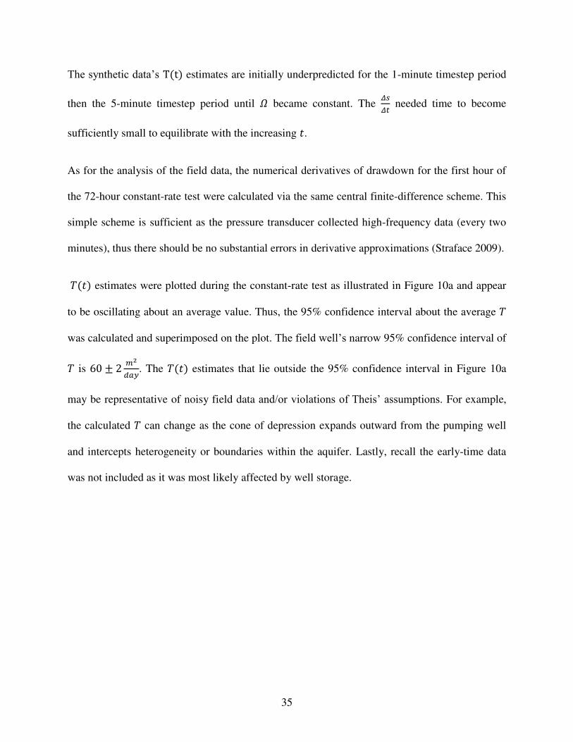
𝑇(𝑡) estimates were plotted during the constant-rate test as illustrated in Figure 10a and appear
to be oscillating about an average value. Thus, the 95% confidence interval about the average 𝑇
was calculated and superimposed on the plot. The field well’s narrow 95% confidence interval of 𝑇 is 60 ± 2 𝑚2𝑑𝑎𝑦. The 𝑇(𝑡) estimates that lie outside the 95% confidence interval in Figure 10a
may be representative of noisy field data and/or violations of Theis’ assumptions. For example,
the calculated 𝑇 can change as the cone of depression expands outward from the pumping well
and intercepts heterogeneity or boundaries within the aquifer. Lastly, recall the early-time data
was not included as it was most likely affected by well storage.

36
Figure 10a – 𝑇(𝑡) estimates, the average, and
95% confidence interval of the field well’s constant-rate test using Equation 18
Figure 10b – 𝛺 estimates, the average, and 95%
confidence interval of the field well’s constant-
rate test using Equation 19
The 𝑇(𝑡) plot and the Ω 𝑣𝑠 𝑡 plot shown in Figure 10b appear to inversely mirror each other;
notice the spikes at 𝑡 ≈ 25𝑚𝑖𝑛 and the sinusoidal wave starting at 𝑡 ≈ 35𝑚𝑖𝑛. This makes sense
as 𝑇(𝑡) is inversely proportional to Ω in Equation 18. It is also important to realize that Ω, a
product of two transient parameters, remains essentially constant during the aquifer test. In fact,
the field well’s narrow 95% confidence interval of Ω is 5 ± 0.2 𝑚.
Errors in the application of these methods should be minimal as most of the time series was used,
effectively removing the risk of analyzing an anomalous data point by mistake (Singh 2002).
Some standard graphical methods, for instance, recommend selecting only one point in each of
the steps of a step-drawdown test, but this increases the likelihood of selecting that erroneous
data (Kawecki 1995). Still, it is recommended to report a confidence interval of 𝑇 to portray the
estimate’s reliability. Moreover, there may be difficulties in maintaining precise pumping rates in
the field if a variable frequency drive submersible pump is not used. Likewise, it might be hard
to record accurate water level measurements in the field if a pressure transducer is not used.
37
4.2.2 Via Fitting a Trendline
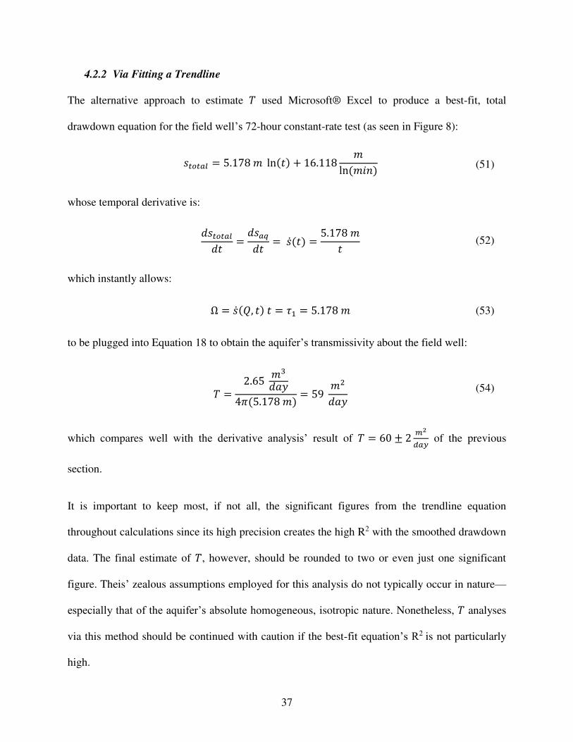
The alternative approach to estimate 𝑇 used Microsoft® Excel to produce a best-fit, total
drawdown equation for the field well’s 72-hour constant-rate test (as seen in Figure 8):
𝑠𝑡𝑜𝑡𝑎𝑙 = 5.178 𝑚 ln(𝑡) + 16.118 𝑚ln (𝑚𝑖𝑛) (51)
whose temporal derivative is:
𝑑𝑠𝑡𝑜𝑡𝑎𝑙𝑑𝑡 = 𝑑𝑠𝑎𝑞𝑑𝑡 = �̇�(𝑡) = 5.178 𝑚𝑡 (52)
which instantly allows:
Ω = �̇�(𝑄, 𝑡) 𝑡 = 𝜏1 = 5.178 𝑚 (53)
to be plugged into Equation 18 to obtain the aquifer’s transmissivity about the field well:
𝑇 = 2.65 𝑚3𝑑𝑎𝑦4𝜋(5.178 𝑚) = 59 𝑚2𝑑𝑎𝑦 (54)
which compares well with the derivative analysis’ result of 𝑇 = 60 ± 2 𝑚2𝑑𝑎𝑦 of the previous
section.
It is important to keep most, if not all, the significant figures from the trendline equation
throughout calculations since its high precision creates the high R2 with the smoothed drawdown
data. The final estimate of 𝑇, however, should be rounded to two or even just one significant
figure. Theis’ zealous assumptions employed for this analysis do not typically occur in nature—
especially that of the aquifer’s absolute homogeneous, isotropic nature. Nonetheless, 𝑇 analyses
via this method should be continued with caution if the best-fit equation’s R2 is not particularly
high.

38
4.3 Rorabaugh and Jacob’s Well-Loss Coefficient and Well-Loss Exponent
4.3.1 Rorabaugh’s Assumption (𝟐 ≤ 𝒏 ≤ 𝟐. 𝟖)
The field well’s dataset, unfortunately, could not be analyzed with the proposed, variable-𝑛
methods since the 𝑄1 was not low enough to assume 𝑠𝑤(𝑄1) ≈ 0. Synthetic data was created for
verification analysis, anyway. Three independent constant-rate tests at a single well were
modeled via Rorabaugh’s total drawdown equation (Equation 4) while varying the predefined 𝐶𝑅
and 𝑛 values. Table 1 lists the predefined aquifer parameters and pumping rates. Table 2 lists the
predefined well-loss parameters along with the results of the proposed methods—specifically, 𝑛
estimates via Equation 37 (𝑛𝑚𝑜𝑑𝑒𝑙) and 𝑛𝑐𝑜𝑟𝑟𝑒𝑐𝑡𝑒𝑑 via Equation 43. The results are simply
reported because each estimate appeared constant for every 𝑡 throughout the 60-minute aquifer
test. It was also observed that changing the predefined 𝐶𝑅 value did not alter the results. This
makes sense as Equation 37 and Equation 43 are not functions of 𝐶𝑅. Even further, the results
were unaffected when predefined 𝑇 and 𝑟2𝑆 values were varied, which was expected as the 𝐵(𝑡∗) terms were also cleared from the final 𝑛𝑚𝑜𝑑𝑒𝑙 and 𝐶𝑅 equations.
Table 2 – Predefined Well-Loss Parameters and Solution Results
for all 𝑪𝑹_𝒑𝒓𝒆𝒅𝒆𝒇𝒊𝒏𝒆𝒅 𝒏𝒑𝒓𝒆𝒅𝒆𝒇𝒊𝒏𝒆𝒅 𝑛𝑚𝑜𝑑𝑒𝑙 𝑛𝑐𝑜𝑟𝑟𝑒𝑐𝑡𝑒𝑑
2 2.114 1.993
2.2 2.284 2.192
2.4 2.460 2.394
2.6 2.643 2.596
2.8 2.830 2.798
The synthetic data itself did not make the 𝐶𝑅𝑄1𝑛 ≈ 0 assumption during the first independent
constant-rate test. Only the proposed methodology made this assumption in order to resolve an
analytical, closed-form solution for 𝑛. This discrepancy will not allow the proposed solutions to
39
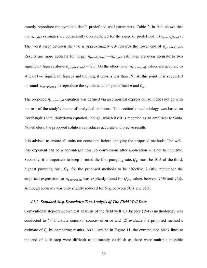
exactly reproduce the synthetic data’s predefined well parameters. Table 2, in fact, shows that
the 𝑛𝑚𝑜𝑑𝑒𝑙 estimates are consistently overpredicted for the range of predefined 𝑛 (𝑛𝑝𝑟𝑒𝑑𝑒𝑓𝑖𝑛𝑒𝑑) .
The worst error between the two is approximately 6% towards the lower end of 𝑛𝑝𝑟𝑒𝑑𝑒𝑓𝑖𝑛𝑒𝑑.
Results are more accurate for larger 𝑛𝑝𝑟𝑒𝑑𝑒𝑓𝑖𝑛𝑒𝑑—𝑛𝑚𝑜𝑑𝑒𝑙 estimates are even accurate to two
significant figures above 𝑛𝑝𝑟𝑒𝑑𝑒𝑓𝑖𝑒𝑛𝑑 = 2.5. On the other hand, 𝑛𝑐𝑜𝑟𝑟𝑒𝑐𝑡𝑒𝑑 values are accurate to
at least two significant figures and the largest error is less than 1%. At this point, it is suggested
to round 𝑛𝑐𝑜𝑟𝑟𝑒𝑐𝑡𝑒𝑑 to reproduce the synthetic data’s predefined 𝑛 and 𝐶𝑅.
The proposed 𝑛𝑐𝑜𝑟𝑟𝑒𝑐𝑡𝑒𝑑 equation was defined via an empirical expression, so it does not go with
the rest of the study’s theme of analytical solutions. This section’s methodology was based on
Rorabaugh’s total drawdown equation, though, which itself is regarded as an empirical formula.
Nonetheless, the proposed solution reproduces accurate and precise results.
It is advised to ensure all units are consistent before applying the proposed methods. The well-
loss exponent can be a non-integer now, so conversions after application will not be intuitive.
Secondly, it is important to keep in mind the first pumping rate, 𝑄1, must be 10% of the third,
highest pumping rate, 𝑄3, for the proposed methods to be effective. Lastly, remember the
empirical expression for 𝑛𝑐𝑜𝑟𝑟𝑒𝑐𝑡𝑒𝑑 was explicitly found for 𝑄2% values between 75% and 95%.
Although accuracy was only slightly reduced for 𝑄2% between 50% and 65%.
4.3.2 Standard Step-Drawdown Test Analysis of The Field Well Data
Conventional step-drawdown test analysis of the field well via Jacob’s (1947) methodology was
conducted to (1) illustrate common sources of error and (2) evaluate the proposed method’s
estimate of 𝐶𝐽 by comparing results. As illustrated in Figure 11, the extrapolated black lines at
the end of each step were difficult to ultimately establish as there were multiple possible

40
combinations of end points that would produce an adequate extrapolation. As the endpoints
changed, so did the results via Jacob’s methodology. The proposed method, on the other hand,
will procure a single 𝐶𝐽 estimate that should be obtainable between different personnel
performing the calculations. Figure 11 also shows the values for ∆𝑠𝑖 and ∆𝑄𝑖 used in the
calculation for the step-drawdown test’s 𝐶𝐽 [T2/L5]:
𝐶𝐽 = (∆𝑠𝑖−1 𝑄𝑖−1⁄ ) + (∆𝑠𝑖 𝑄𝑖⁄ )∆𝑄𝑖−1 + ∆𝑄𝑖 (55)
Unfortunately, none of the steps reached a stable drawdown before the next pumping rate was
initiated. These premature steps would most likely produce an overpredicted estimate of the step-
drawdown test’s 𝐶𝐽 as the steep slopes would make the ∆𝑠𝑖 values larger than actual. Therefore,
the proposed method’s 𝐶𝐽 estimate should be less than the step-drawdown test’s 𝐶𝐽 of
4.6x10⁻⁷ day2m5 , which indicates “mild deterioration” of the well via Walton (1962) in Appendix I.
The step-drawdown test’s 𝐶𝐽 would cause 5.6 meters of excess drawdown when 𝑄 = 3,500 𝑚3𝑑𝑎𝑦.
Figure 11 – Jacob’s (1947) traditional methodology for the step-drawdown test’s 𝐶𝐽

41
4.3.3 Jacob’s Assumption (𝒏 = 𝟐)
Jacob’s well-loss coefficient of the field well was estimated via Equation 26 and the first step (60
minutes long) of a step-drawdown test and the first 60 minutes of a constant-rate test. The water-
level returned to its initial, static position between the step and constant-rate tests, so the two can
be considered “independent constant-rate tests”. The two tests’ specific drawdown curves are
plotted in Figure 12a while Equation 26 was used to plot the field well’s 𝐶𝐽 in Figure 12b.
Figure 12a - The field well’s s/Q vs 𝑡 plot
Figure 12b – The field well’s 𝐶𝐽 vs 𝑡 plot
Figure 12a was plotted on a semi-log plot to illustrate how sw affects the specific drawdown
lines. It seems well-loss effects are present during the Constant-Rate Test because of the offset
between the two siQi lines; if there was no well loss, the two lines would overlap. As for Figure
12b, the field well’s CJ converges to its lowest value as the differences between the siQi lines
stabilize. This stabilization occurs when 𝐵(𝑡∗) approaches its maximum value in Jacob’s total
drawdown equation (Equation 23); 𝐵(𝑡∗) becomes approximately constant in the field after a
sufficiently long period of pumping (Labadie 1975). Therefore, the proposed method’s final 𝐶𝐽 =2.4x10⁻⁷ day2m5 (which is indeed smaller than Jacob’s 𝐶 of 4.6x10⁻⁷ day2m5 ) was anticipated as
explained in Section 4.3.2. The presented method’s value would be considered appropriate by
42
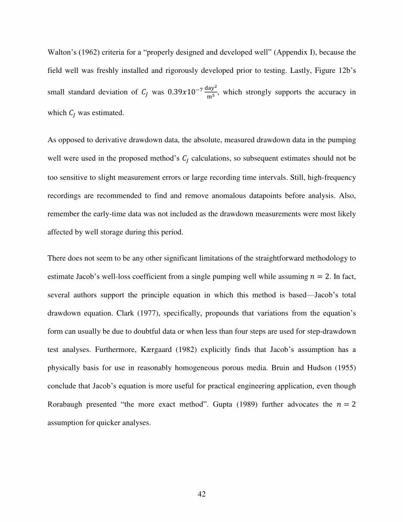
Walton’s (1962) criteria for a “properly designed and developed well” (Appendix I), because the
field well was freshly installed and rigorously developed prior to testing. Lastly, Figure 12b’s
small standard deviation of 𝐶𝐽 was 0.39𝑥10−7 day2m5 , which strongly supports the accuracy in
which 𝐶𝐽 was estimated.
As opposed to derivative drawdown data, the absolute, measured drawdown data in the pumping
well were used in the proposed method’s 𝐶𝐽 calculations, so subsequent estimates should not be
too sensitive to slight measurement errors or large recording time intervals. Still, high-frequency
recordings are recommended to find and remove anomalous datapoints before analysis. Also,
remember the early-time data was not included as the drawdown measurements were most likely
affected by well storage during this period.
There does not seem to be any other significant limitations of the straightforward methodology to
estimate Jacob’s well-loss coefficient from a single pumping well while assuming 𝑛 = 2. In fact,
several authors support the principle equation in which this method is based—Jacob’s total
drawdown equation. Clark (1977), specifically, propounds that variations from the equation’s
form can usually be due to doubtful data or when less than four steps are used for step-drawdown
test analyses. Furthermore, Kærgaard (1982) explicitly finds that Jacob’s assumption has a
physically basis for use in reasonably homogeneous porous media. Bruin and Hudson (1955)
conclude that Jacob’s equation is more useful for practical engineering application, even though
Rorabaugh presented “the more exact method”. Gupta (1989) further advocates the 𝑛 = 2
assumption for quicker analyses.
43
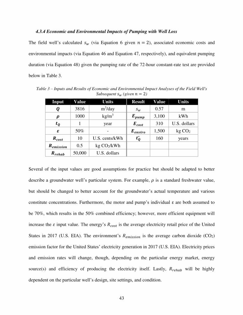
4.3.4 Economic and Environmental Impacts of Pumping with Well Loss
The field well’s calculated 𝑠𝑤 (via Equation 6 given 𝑛 = 2), associated economic costs and
environmental impacts (via Equation 46 and Equation 47, respectively), and equivalent pumping
duration (via Equation 48) given the pumping rate of the 72-hour constant-rate test are provided
below in Table 3.
Table 3 – Inputs and Results of Economic and Environmental Impact Analyses of the Field Well's
Subsequent 𝑠𝑤 (given 𝑛 = 2)
Input Value Units Result Value Units 𝑸 3816 m3/day 𝑠𝑤 0.57 m 𝝆 1000 kg/m3 𝑬𝒑𝒖𝒎𝒑 3,100 kWh 𝒕𝑸 1 year 𝑬𝒄𝒐𝒔𝒕 310 U.S. dollars 𝜺 50% - 𝑬𝒆𝒏𝒗𝒊𝒓𝒐 1,500 kg CO2 𝑹𝒄𝒐𝒔𝒕 10 U.S. cents/kWh 𝒕𝑸∗ 160 years 𝑹𝒆𝒎𝒊𝒔𝒔𝒊𝒐𝒏 0.5 kg CO2/kWh 𝑹𝒓𝒆𝒉𝒂𝒃 50,000 U.S. dollars
Several of the input values are good assumptions for practice but should be adapted to better
describe a groundwater well’s particular system. For example, 𝜌 is a standard freshwater value,
but should be changed to better account for the groundwater’s actual temperature and various
constitute concentrations. Furthermore, the motor and pump’s individual ε are both assumed to
be 70%, which results in the 50% combined efficiency; however, more efficient equipment will
increase the 𝜀 input value. The energy’s 𝑅𝑐𝑜𝑠𝑡 is the average electricity retail price of the United
States in 2017 (U.S. EIA). The environment’s 𝑅𝑒𝑚𝑖𝑠𝑠𝑖𝑜𝑛 is the average carbon dioxide (CO2)
emission factor for the United States’ electricity generation in 2017 (U.S. EIA). Electricity prices
and emission rates will change, though, depending on the particular energy market, energy
source(s) and efficiency of producing the electricity itself. Lastly, 𝑅𝑟𝑒ℎ𝑎𝑏 will be highly
dependent on the particular well’s design, site settings, and condition.

44
The calculated 𝑠𝑤 for the 72-hour constant-rate test is low for a newly installed and rigorously
developed well—𝑠𝑤 accounts for approximately just 1.5% of 𝑠𝑡𝑜𝑡𝑎𝑙 after 60 minutes of pumping.
The associated economic and environmental impacts of pumping the field well’s additional 𝑇𝐷𝐻
caused by 𝑠𝑤 for a year suggest the pumping well is performing efficiently with relatively low
impacts. For example, the 1,500 kg of CO2 emissions is equivalent to just 0.2 U.S. homes’
energy use for one year (U.S. EPA). Lastly, the calculated 310 dollars/year to pump the field
well’s minimal well loss suggests rehabilitation is not necessary given the current conditions and
a practical design period of a well system, which is typically less than the estimated 𝑡𝑄∗ =160 𝑦𝑒𝑎𝑟𝑠. As a result, Equation 49 [𝑡𝑄 ≥ 𝑡𝑄∗ ] should not be true. Nevertheless, regular aquifer
tests should be conducted every few years to reassess well-loss coefficient estimates due to the
perpetual nature of well aging/clogging.
45
5. CONCLUSION
This section summarizes the motivation behind and the implications of the proposed methods.
Suggestions for future work are also presented.
5.1 Summary
Well loss unnecessarily increases the energy required to produce groundwater. Thus, estimating
and ensuring well loss is minimized is important for reducing the costs and carbon footprint of
pumping. Standard methods exist to quantify the aquifer- and well-loss contributions of
drawdown, but these methods have limitations. A few examples include step-test analyses, which
are highly subjective, and computer-based techniques, which are rather involved.
Straightforward, less subjective methods were developed to overcome the limitations of standard
methods. Specifically, derivative analysis and trendline functions were used to accurately and
objectively estimate the aquifer’s transmissivity about a single pumping well. The field well’s
transmissivity had a narrow confidence interval, ensuring the accuracy of the methodologies.
Furthermore, groundwater professionals and students analyzing the same drawdown data should
obtain the same transmissivity estimates with the proposed methods. Other methodologies were
proposed to simply estimate Jacob’s well-loss coefficient or Rorabaugh’s well-loss coefficient
and well-loss exponent via independent constant-rate tests at a single pumping well. More
precisely, a simple system of equations, an elementary assumption, and an optional regression
model were employed to estimate the well-loss parameter(s). For example, Jacob’s well-loss
coefficient of the field well embodied a low standard deviation, illustrating the reliability of the
method.

46
The well-loss parameter(s) were, then, used to estimate the excess drawdown due to nonlaminar
flows at the design pumping rate. Finally, the equivalent economic costs and environmental
emissions of pumping the well loss were resolved. Hence, the proposed methods facilitate the
use of well loss as a well performance metric. When well loss and its impacts become too large,
further development of a new well/rehabilitation of a preexisting well is advised. The pumping
well’s development/rehabilitation will reduce well loss, energy requirements, and the associated
economic and environmental costs of groundwater production.
5.2 Recommendations for Future Work
This section suggests several potential avenues of future efforts to increase the efficacy of the
proposed methods. Applying the solutions to other groundwater wells in a variety of different
hydrogeologic conditions can provide further highlights of the methods’ advantages. More
applications of the proposed methods can also offer insight to other limitations the author is
unaware of at this time.
Simply applying the solutions to more groundwater wells completed in a confined aquifer can
refine the application of the proposed methods. This argument is taken from a purely statistical
standpoint as the methods were applied to only one field dataset. The field well’s aquifer test
data was very clean. Other wells of similar design in similar aquifers will undoubtedly not
provide such ideal data, which can considerably affect the solutions’ accuracy. Thankfully,
Hemenway Groundwater Engineering is planning to run three independent constant-rate tests at a
groundwater production well in Highlands Ranch, Colorado in Summer 2019. The proposed
methods should be applied to the upcoming data in an attempt to find the prevalent sources of
error and potentially crucial limitations of the methods’ application.
47
Another good step would be to start analyzing unconfined aquifer test data. Theoretically, Theis’
equation can be used to describe an unconfined aquifer’s drawdown response to pumping once
delayed drainage has passed and if the change in the saturated thickness remains small (Theis
1935). It is therefore advised to apply the proposed methods to aquifer test data from a well in an
unconfined aquifer to validate the method’s diverse applicability.
Lastly, automating the proposed methods seems crucial for the modern world’s trajectory
towards big-data and energy efficiency (Ronayne et al. 2017; Karimi Askarani et al. 2018).
Developing a program with a user-friendly graphical user interface should make estimates of
aquifer and well parameters much quicker and more readily available. Analyses of economic and
environmental could be standardized, too, for more effective groundwater well installation and
rehabilitation efforts. It is therefore recommended to develop a computer-based program for the
automated analyses of aquifer test data via the proposed methods.

48
REFERENCES
Bierschenk, W.H. 1963. Determining well efficiency by multiple step-drawdown tests.
International Association of Scientific Hydrology: 493-507.
Bruin, J. and H.E Hudson. 1955. Selected methods for pumping test analysis. Illinois State Water
Survey.
Clark, L. 1977. The analysis and planning of step drawdown tests. Quarterly Journal of
Engineering Geology and Hydrogeology 10, no. 2: 125-143.
Cooper, H.H. and C.E. Jacob. 1946. A generalized graphical method for evaluating formation
constants and summarizing well field history. Transactions of the American Geophysical Union
27, no. 4: 526-534
Eden, R.N. and C.P. Hazel. 1973. Computer and graphical analysis of variable discharge
pumping test of wells. The Institute of Engineers Australia.
Fetter, C.W. 2001. Applied Hydrogeology. Upper Saddle River, New Jersey: Prentice Hall.
Gupta, A.D. 1989. On analysis of step‐drawdown data. Groundwater 27, no. 6: 874-881.
Hanna, T.M., P.G. Ivanci and W.A. Creswell. 2003. Aquifer analysis and proper well
development to maximize pumping capacity in alluvial wells. Water Well Journal 57: 34-37.
Hantush, M.S., 1964. Hydraulics of wells. Advances in Hydroscience 1: 281-432.
Hemenway, C. 2018. Personal conversation with author.
Houben, G.J. 2003. Iron Oxide Incrustations in Wells, Part 1: Genesis, Mineralogy and
Geochemistry. Applied Geochemistry 18, no. 6:927–939.
Houben, G.J. 2015. Hydraulics of water wells—flow laws and influence of geometry.
Hydrogeology Journal 23, no. 8: 1633-1657.

49
Houben G.J. and C. Treskatis. 2007. Water Well Rehabilitation and Reconstruction. New York:
McGraw Hill.
Houben G.J. and S. Hauschild. 2011. Numerical modelling of the near-field hydraulics of water
wells. Ground Water 49, no. 4:570–575
Houben, G.J., J. Wachenhausen and C.R.G. Morel. 2018. Effects of ageing on the hydraulics of
water wells and the influence of non-Darcy flow. Hydrogeology Journal 26, no. 4: 1285-1294.
Istok, Jonathan D., and Karen J. Dawson. 1991. Aquifer Testing: Design and Analysis of
Pumping and Slug Tests, 1st ed. Boca Raton, Florida: CRC Press, 2014
Jacob, C.E. 1947. Drawdown Test to Determine the Effective Radius of an Artesian Well,
Transactions of the American Society of Civil Engineers 112: 1047-1070.
Jha, M.K., A. Kumar, G. Nanda and G. Bhatt. 2006. Evaluation of traditional and nontraditional
optimization techniques for determining well parameters from step-drawdown test data. Journal
of Hydrologic Engineering 11, no. 6: 617-630.
Kærgaard, H. 1982. The step-drawdown test and non-Darcian flow: a critical review of theory,
methods and practice. Hydrology Research 13, no. 4: 247-256.
Karimi Askarani, K., E.B. Stockwell, K.R. Piontek, and T.C. Sale. 2018. Thermal Monitoring of
Natural Source Zone Depletion. Groundwater Monitoring & Remediation 38, no. 3: 43-52.
Kawecki, M.W. 1995. Meaningful interpretation of step‐drawdown tests. Groundwater 33, no. 1:
23-32.
Konikow, L.F. 2015. Long‐term groundwater depletion in the United States. Groundwater 53,
no. 1:2-9.
Kruseman, G.P. and N.A. de Ridder. 2000. Analysis and Evaluation of Pumping Test Data,
Second Edition (Completely Revised). Wageningen: International Institute for Land Reclamation
and Improvement.
Labadie, J.W. and O.J. Helweg. 1975. Step‐drawdown test analysis by computer. Groundwater
13, no. 5: 438-444.

50
Lennox, D.H. 1966. Analysis and application of step-drawdown test. Journal of the Hydraulics
Division 92, no. 6: 25-48.
Lennox, D.H. 1968. Step‐Drawdown Test Needs Critical Review by Joe L. Mogg–July‐August, 1968. Groundwater 7, no. 6: 35-36.
Lewis, A.R., M.J. Ronayne, and T.C. Sale. 2016. Estimating aquifer properties using derivative
analysis of water level time series from active well fields. Groundwater 54, no. 3: 414-424.
Mays, L. W. 2012. Ground and Surface Water Hydrology. Hoboken: John Wiley & Sons.
Memon, A.A., N.A Memon and K.A.M.R.A.N. Ansari. 2012. Determination of turbulence
coefficient using genetic algorithms. Mehran University Research Journal of Engineering and
Technology 31 no. 4: 651-658.
Mogg, J.L. 1969. Step‐Drawdown Test Needs Critical Reviewa. Groundwater 7, no 1: 28-34.
Ronayne, M., T.C. Sale, J. Suter. and D. Shugert. (2017). Evaluating the energy cost of
groundwater production in the Denver Basin aquifers, Colorado Water Newsletter 34, no. 5: 5-8.
Rorabaugh, M.I. 1953. Graphical and theoretical analysis of step-drawdown test of artesian well.
Proceedings of the American Society of Civil Engineers 79, no. 12: 1-23.
Sheahan, N. T. 1971. Type‐curve solution of step‐drawdown test. Groundwater 9, no. 1: 25-29.
Shekhar, S. 2006. An approach to interpretation of step drawdown tests. Hydrogeology Journal
14, no. 6: 1018-1027.
Singh, S.K. 2002. Well loss estimation: Variable pumping replacing step drawdown test. Journal
of Hydraulic Engineering 128, no. 3: 343-348.
Sterrett, R. J. 2007. Groundwater and Wells, 3rd ed. New Brighton, Minnesota: Johnson Screens.
Straface, S. 2009. Estimation of transmissivity and storage coefficient by means of a derivative
method using the early-time drawdown. Hydrogeology Journal 17, no. 7: 1679.

51
Theis, C.V. 1935. The relation between the lowering of the piezometric surface and the rate and
duration of discharge of a well using groundwater storage. Transactions of the American
Geophysical Union 16: 519–524.
United States Energy Information Administration (U.S. EIA). 2019. United Electricity Profile
2017. Accessed 1 May 2019, < https://www.eia.gov/electricity/state/unitedstates/index.php>.
United States Environmental Protection Agency (U.S. EPA). 2019. Greenhouse Gas
Equivalencies Calculator. Accessed 1 May 2019, <https://www.epa.gov/energy/greenhouse-gas-
equivalencies-calculator>.
Walton, W.C. 1962. Selected analytical methods for well and aquifer evaluation. Bulletin
(Illinois State Water Survey) 49.
Wendling, G., R.P Chapuis and D.E. Gill. 1997. Quantifying the effects of well development in
unconsolidated material. Groundwater 35, no. 3: 387-393.
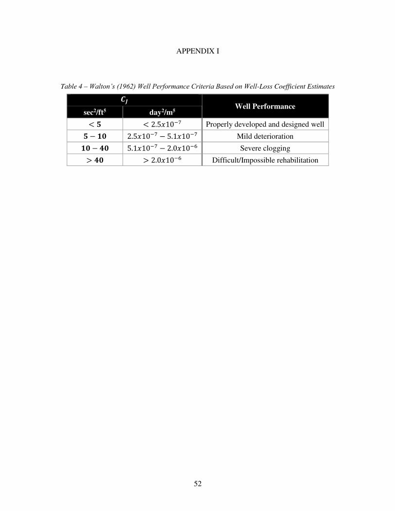
52
APPENDIX I
Table 4 – Walton’s (1962) Well Performance Criteria Based on Well-Loss Coefficient Estimates 𝑪𝑱
Well Performance sec2/ft5 day2/m5 < 𝟓 < 2.5𝑥10−7 Properly developed and designed well 𝟓 − 𝟏𝟎 2.5𝑥10−7 − 5.1𝑥10−7 Mild deterioration 𝟏𝟎 − 𝟒𝟎 5.1𝑥10−7 − 2.0𝑥10−6 Severe clogging > 𝟒𝟎 > 2.0𝑥10−6 Difficult/Impossible rehabilitation

53
LIST OF ABBREVIATIONS
Abbreviation Dimensions* Description 𝐵(𝑡) T/L2 aquifer-loss coefficient
CO2 - carbon dioxide 𝐶𝐽 T2/L5 Jacob’s well-loss coefficient 𝐶𝑅 Tn/L3n-1 Rorabaugh’s well-loss coefficient 𝐶𝑅_𝑐𝑜𝑟𝑟𝑒𝑐𝑡𝑒𝑑 Tn/L3n-1 refined 𝐶𝑅 estimate via Equation 44 𝑑𝑠𝑡𝑜𝑡𝑎𝑙𝑑𝑡 or �̇�(𝑄, 𝑡) L/T derivative drawdown 𝐷𝑇𝑊𝑠𝑡𝑎𝑡𝑖𝑐 L depth from the well head to the static groundwater level
prior to pumping 𝐸𝑐𝑜𝑠𝑡 currency economic impact (or “cost”) of supplying the extra required energy to pump the excess drawdown 𝐸𝑒𝑛𝑣𝑖𝑟𝑜 M the environmental impact (or “emissions”) of using the extra required energy to pump the excess drawdown 𝐸𝑝𝑢𝑚𝑝 M L2/T2 extra required energy to pump the excess drawdown 𝐸𝑤(𝑄, 𝑡) - well efficiency 𝑔 L/T2 acceleration due to gravity ℎ𝑓 L friction losses contributable to conveyance ℎ𝑝 L pressure head required for sufficient discharge at the point
of use ℎ𝑢𝑠𝑒 L the elevation change from the well head to the point of use 𝑖 - index of list [1, 2, or 3] 𝑚 - variable of integration 𝑛 - Rorabaugh’s well-loss exponent 𝑛𝑐𝑜𝑟𝑟𝑒𝑐𝑡𝑒𝑑 - refined 𝑛 estimate via Equation 43 𝑛𝑚𝑜𝑑𝑒𝑙 - modeled 𝑛 via Equation 37 𝑛𝑝𝑟𝑒𝑑𝑒𝑓𝑖𝑛𝑒𝑑 - synthetic data’s predefined 𝑛 value 𝑄2% - 𝑄2’s percentage of 𝑄3 𝑄 L3/T pumping rate 𝑄𝑖 L3/T pumping rate during the 𝑖th aquifer test 𝑟 L radial distance from the pumping well to a point of interest 𝑅𝑐𝑜𝑠𝑡 currency/ cost rate of energy
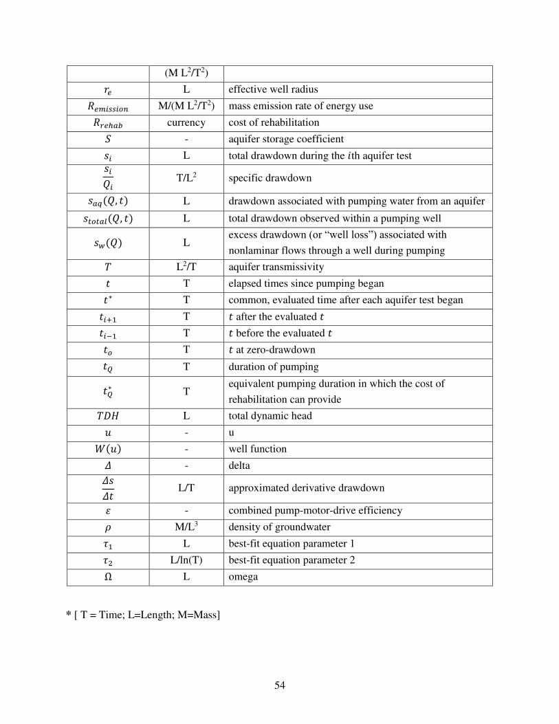
54
(M L2/T2) 𝑟𝑒 L effective well radius 𝑅𝑒𝑚𝑖𝑠𝑠𝑖𝑜𝑛 M/(M L2/T2) mass emission rate of energy use 𝑅𝑟𝑒ℎ𝑎𝑏 currency cost of rehabilitation 𝑆 - aquifer storage coefficient 𝑠𝑖 L total drawdown during the 𝑖th aquifer test 𝑠𝑖𝑄𝑖 T/L2 specific drawdown 𝑠𝑎𝑞(𝑄, 𝑡) L drawdown associated with pumping water from an aquifer 𝑠𝑡𝑜𝑡𝑎𝑙(𝑄, 𝑡) L total drawdown observed within a pumping well 𝑠𝑤(𝑄) L excess drawdown (or “well loss”) associated with nonlaminar flows through a well during pumping 𝑇 L2/T aquifer transmissivity 𝑡 T elapsed times since pumping began 𝑡∗ T common, evaluated time after each aquifer test began 𝑡𝑖+1 T 𝑡 after the evaluated 𝑡 𝑡𝑖−1 T 𝑡 before the evaluated 𝑡 𝑡𝑜 T 𝑡 at zero-drawdown 𝑡𝑄 T duration of pumping 𝑡𝑄∗ T equivalent pumping duration in which the cost of
rehabilitation can provide 𝑇𝐷𝐻 L total dynamic head 𝑢 - u 𝑊(𝑢) - well function 𝛥 - delta 𝛥𝑠𝛥𝑡 L/T approximated derivative drawdown 𝜀 - combined pump-motor-drive efficiency 𝜌 M/L3 density of groundwater 𝜏1 L best-fit equation parameter 1 𝜏2 L/ln(T) best-fit equation parameter 2 Ω L omega
* [ T = Time; L=Length; M=Mass]