thermophysical and compositional properties of natural gas hydrate
TRANSCRIPT

Odd Ivar Levik
Thermophysical and Compositional
Properties of Natural Gas Hydrate
Thesis submitted in partial ful�llment
of the requirements for the degree of
Doktor Ingeni�r of the
Norwegian University of Science and Technology
Department of Petroleum Engineering and Applied Geophysics
September 2000

ii

Abstract
Thermophysical properties (dissociation enthalpy, heat capacity, metastabil-ity) and compositional properties (hydrate number, free water and fraction-ation) of natural gas hydrate were studied experimentally on samples thatcontained large amounts of ice. Methods for continuous hydrate produc-tion and sampling, and for quanti�cation of the properties were developed.Hydrate was produced from a natural gas of ethane (5 %mol) and propane(3 %mol) in methane.
A low temperature scanning calorimetry method was developed to measuredissociation enthalpy, heat capacity, hydrate number and free water (ice).During the analysis, the hydrate samples were pressurized to 1.7 MPa withmethane and the system operated between the hydrate equilibrium curvesof methane and the hydrate forming natural gas. A sample conditioningprocedure eliminated thermal e�ects of desorption as the ice melted. Des-orption occurred since the samples were produced and refrigerated to 255 Kunder a natural gas pressure of 6-10 MPa, but were analyzed and meltedunder a methane pressure of 1.7 MPa.
A low temperature isothermal calorimetry method was developed to quantifythe metastability properties. Metastability was con�rmed for temperaturesup to 268 K and quanti�ed in terms of the low dissociation rate.
Fractionation data were obtained in the range 3.0 to 7.5 MPa and for sub-coolings between 2 and 16 K. High pressure and large subcooling is desirableto suppress fractionation. A fractionation model was proposed. The modelcoincides with the van der Waals-Platteeuw model for zero subcooling. Nofractionation is assumed for hypothetical hydrate formation at in�nite driv-ing force (subcooling). Between these two extremes an exponential term wasused to describe the fractionation. The model predicted fractionation withan accuracy of about 1%abs corresponding to 1-10%rel.
iii

iv ABSTRACT

Acknowledgments
First of all I thank my supervisor, Professor J�on Steinar Gudmundsson, whogave me the opportunity to learn and with whom I discussed matters farmore important than hydrates.
Then I thank Vibeke Andersson, my friend and fellow Dr.Ing. student duringthe last few years, who always knew what I did not.
Associate Professor Mahmut Parlaktuna, who came from the Middle EastTechnical University, I thank for all his help in laboratory, for sharing hisexperiences and for saying \let's do it".
I thank Professor Jean-Pierre Monfort of the National School of ChemicalEngineering in Toulouse for his countless e�orts in my interest and for settingthe standard of hospitality.
Engineers Ivar Bjerkan, Gunnar Bjerkan, �Age Sivertsen and Roger Over�a atthe workshop played important roles, especially during construction periods,but also in everyday operations.
I also thank other members of Professor Gudmundsson's group, notablyDr.Ing. student Elling Sletfjerding and Post-Doc. fellow Ismail Durgut, whotouched the keyboard in all the secret places, so that the computer ERRORmessages went away for a while. Dr.Ing. student Aftab Ali Khokhar too wasa member of our group, but carried out most of his work at the ColoradoSchool of Mines. Our discussions always brought me one step ahead.
Dr. William R. (Bill) Parrish of Phillips Petroleum is sincerely thanked forsupport and valuable discussions on calorimetry.
Mr. Jean-Louis Peytavy of Elf E&P in Pau gave valuable help by providingnecessary equipment to the fractionation laboratory.
v

vi ACKNOWLEDGMENTS
Dr.Ing. Geir Ultveit HaUgEn was sort of a�liated to the Gudmundssongroup too, in the evenings. Good for me.
Aker Engineering is especially thanked for the three-year stipend I receivedto study at NTNU. TOTAL Norge is especially thanked for the one-yearstipend I received to study at the National School of Chemical Engineeringin Toulouse.
The present work was given �nancial support by the partners of the NGHat NTNU joint industry project; Aker Engineering, Amerada-Hess, AtlanticRich�eld, Fortum Petroleum, Phillips Petroleum, Shell International Explo-ration & Production and TOTAL Norge. The Nordic Energy Research Pro-gram gave me the opportunity to visit the Technical University of Denmark.
But still I would have reached nowhere without my parents Maj and Martinwho supported, encouraged and loved me whatever I wanted to do (Well...,I was not allowed to eat Karlson's Glue and to dive from \M/T Fenborg"in the Paci�c Ocean). I will try to be an equally good father for littleAnnastina. I thank my brother Anders for cheering me up and for the goodtalks and for all those tunes and lyrics.
And to my wife Evy: Thank you for your concern and patience - I lookforward to catching up.
We did have some real good timesI remember them
Quotation from one of Anders' songs

Contents
Abstract iii
Acknowledgements v
Contents vii
List of Tables xi
List of Figures xiii
Nomenclature xv
1 Introduction 1
1.1 Background . . . . . . . . . . . . . . . . . . . . . . . . . . . . 11.1.1 Storage and Transport of Natural Gas Using Hydrate 11.1.2 Emerging Scenarios . . . . . . . . . . . . . . . . . . . 2
1.2 Topics . . . . . . . . . . . . . . . . . . . . . . . . . . . . . . . 31.2.1 Problem Statements . . . . . . . . . . . . . . . . . . . 31.2.2 Scopes of Work . . . . . . . . . . . . . . . . . . . . . . 4
2 Thermal and Compositional Properties - Literature Study 5
2.1 Hydrate Composition . . . . . . . . . . . . . . . . . . . . . . 52.2 Heat Flow DSC . . . . . . . . . . . . . . . . . . . . . . . . . . 82.3 Measurements by Calorimetry . . . . . . . . . . . . . . . . . . 12
2.3.1 Measurements by Handa et al. (�h�diss, n and f) . . . 132.3.2 Other Measurements (�hdiss) . . . . . . . . . . . . . . 162.3.3 Non-calorimetric Techniques to Measure n . . . . . . . 17
2.4 Dissociation Enthalpy Models and Correlations . . . . . . . . 172.4.1 The Clausius-Clapeyron Equation . . . . . . . . . . . 172.4.2 Guest Size Dependent Enthalpy Estimation . . . . . . 20
vii

viii CONTENTS
2.4.3 Chemical Potential Model . . . . . . . . . . . . . . . . 222.4.4 Correlations . . . . . . . . . . . . . . . . . . . . . . . . 232.4.5 Dissociation Enthalpy Comparison . . . . . . . . . . . 24
2.5 Speci�c Heat Capacity . . . . . . . . . . . . . . . . . . . . . . 262.5.1 Measurements . . . . . . . . . . . . . . . . . . . . . . 262.5.2 Models and Correlations . . . . . . . . . . . . . . . . . 27
2.6 Thermal Conductivity and Expansivity . . . . . . . . . . . . 292.7 Important Findings . . . . . . . . . . . . . . . . . . . . . . . . 30
3 Metastability - Literature Study 33
3.1 Metastability Concepts . . . . . . . . . . . . . . . . . . . . . . 333.2 Hydrate Metastability Measurements . . . . . . . . . . . . . . 343.3 Hydrate Metastability Models . . . . . . . . . . . . . . . . . . 363.4 Rate of Solid-Solid Transitions . . . . . . . . . . . . . . . . . 393.5 Important Findings . . . . . . . . . . . . . . . . . . . . . . . . 41
4 Fractionation and Driving Force - Literature Study 43
4.1 Fractionation . . . . . . . . . . . . . . . . . . . . . . . . . . . 434.1.1 Fractionation Measurements . . . . . . . . . . . . . . . 434.1.2 Fractionation Model . . . . . . . . . . . . . . . . . . . 454.1.3 Fractionation Simulations . . . . . . . . . . . . . . . . 48
4.2 Driving Force . . . . . . . . . . . . . . . . . . . . . . . . . . . 484.3 Discussion . . . . . . . . . . . . . . . . . . . . . . . . . . . . . 494.4 Important Findings . . . . . . . . . . . . . . . . . . . . . . . . 50
5 Apparatuses 53
5.1 Introduction . . . . . . . . . . . . . . . . . . . . . . . . . . . . 535.2 Flow Loop Laboratory . . . . . . . . . . . . . . . . . . . . . . 54
5.2.1 Conceptual Design . . . . . . . . . . . . . . . . . . . . 545.2.2 Room Temperature . . . . . . . . . . . . . . . . . . . . 555.2.3 Main Units . . . . . . . . . . . . . . . . . . . . . . . . 565.2.4 Utility Units . . . . . . . . . . . . . . . . . . . . . . . 625.2.5 Instrumentation, Regulation and Logging . . . . . . . 655.2.6 Safety . . . . . . . . . . . . . . . . . . . . . . . . . . . 675.2.7 Miscellaneous . . . . . . . . . . . . . . . . . . . . . . . 67
5.3 Cold Laboratory . . . . . . . . . . . . . . . . . . . . . . . . . 685.4 Calorimeter Laboratory . . . . . . . . . . . . . . . . . . . . . 685.5 Climate Laboratory . . . . . . . . . . . . . . . . . . . . . . . 705.6 Batch Reactor Laboratory . . . . . . . . . . . . . . . . . . . . 71
5.6.1 Concept . . . . . . . . . . . . . . . . . . . . . . . . . . 71

CONTENTS ix
5.6.2 Reactor . . . . . . . . . . . . . . . . . . . . . . . . . . 715.6.3 Gas Analysis . . . . . . . . . . . . . . . . . . . . . . . 73
6 Hydrate Sampling and Calorimetry Method 75
6.1 Introduction . . . . . . . . . . . . . . . . . . . . . . . . . . . . 756.2 Method for Continuous Hydrate Production and Sampling . . 766.3 Calorimetric Method . . . . . . . . . . . . . . . . . . . . . . . 77
6.3.1 Introductory Experiments . . . . . . . . . . . . . . . . 786.3.2 Preliminary Calorimetric Method . . . . . . . . . . . . 796.3.3 Criticism of the Preliminary Method . . . . . . . . . . 856.3.4 Final Calorimetric Method . . . . . . . . . . . . . . . 88
6.4 Properties Estimates . . . . . . . . . . . . . . . . . . . . . . . 916.5 Discussion . . . . . . . . . . . . . . . . . . . . . . . . . . . . . 91
6.5.1 Calorimetric Method . . . . . . . . . . . . . . . . . . . 916.5.2 Hydrate Sampling . . . . . . . . . . . . . . . . . . . . 93
6.6 Conclusions . . . . . . . . . . . . . . . . . . . . . . . . . . . . 94
7 Metastability - Results 95
7.1 Introduction . . . . . . . . . . . . . . . . . . . . . . . . . . . . 957.2 Isothermal Calorimetry Method . . . . . . . . . . . . . . . . . 95
7.2.1 E�ect of Temperature . . . . . . . . . . . . . . . . . . 967.2.2 E�ect of Sample Diameter . . . . . . . . . . . . . . . . 97
7.3 Discussion . . . . . . . . . . . . . . . . . . . . . . . . . . . . . 977.3.1 Rate Limitations . . . . . . . . . . . . . . . . . . . . . 977.3.2 E�ect of Temperature and Sample Size . . . . . . . . 997.3.3 E�ect of Pressure . . . . . . . . . . . . . . . . . . . . . 1007.3.4 Blank Run . . . . . . . . . . . . . . . . . . . . . . . . 1007.3.5 Micro Regimes . . . . . . . . . . . . . . . . . . . . . . 1017.3.6 Other Comments . . . . . . . . . . . . . . . . . . . . . 1017.3.7 Speculations on Metastability . . . . . . . . . . . . . . 102
7.4 Conclusions . . . . . . . . . . . . . . . . . . . . . . . . . . . . 103
8 Fractionation - Results 105
8.1 General Fractionation Model . . . . . . . . . . . . . . . . . . 1058.2 Methods . . . . . . . . . . . . . . . . . . . . . . . . . . . . . . 1078.3 Measurements . . . . . . . . . . . . . . . . . . . . . . . . . . . 1098.4 Interpretation of Measurement Results . . . . . . . . . . . . . 112
8.4.1 Driving Force Threshold . . . . . . . . . . . . . . . . . 1128.4.2 System Speci�c Fractionation Model . . . . . . . . . . 1138.4.3 Simulations . . . . . . . . . . . . . . . . . . . . . . . . 115

x CONTENTS
8.5 Discussion . . . . . . . . . . . . . . . . . . . . . . . . . . . . . 1198.5.1 Fractionation Model . . . . . . . . . . . . . . . . . . . 1198.5.2 Calibration and Measurement Errors . . . . . . . . . . 121
8.6 Conclusions . . . . . . . . . . . . . . . . . . . . . . . . . . . . 122
9 Discussion 123
9.1 Advances and Shortcomings . . . . . . . . . . . . . . . . . . . 1239.1.1 Thermal and Compositional Properties . . . . . . . . 1239.1.2 Metastability . . . . . . . . . . . . . . . . . . . . . . . 1249.1.3 Fractionation . . . . . . . . . . . . . . . . . . . . . . . 124
9.2 Further Work . . . . . . . . . . . . . . . . . . . . . . . . . . . 125
10 Conclusions 127
References 129
A Collection of �h�diss and n measurements in the Literature 137
B Experiments and Findings Leading to the Preliminary Calori-
metric Method 141
B.1 Alternative Schemes for a Calorimetric Method . . . . . . . . 141B.2 Individual Tests . . . . . . . . . . . . . . . . . . . . . . . . . . 142
B.2.1 Tests with Natural Gas . . . . . . . . . . . . . . . . . 142B.2.2 Tests with Nitrogen . . . . . . . . . . . . . . . . . . . 143B.2.3 Tests with Methane . . . . . . . . . . . . . . . . . . . 149
C Thermal and Compositional Properties - Estimates 153
D Determination of Fractionation Model Parameters 157
E List of Publications 164

List of Tables
2.1 Comparison of guest and cage diameters . . . . . . . . . . . . 72.2 �h�diss measurements . . . . . . . . . . . . . . . . . . . . . . . 152.3 �hdiss measurements . . . . . . . . . . . . . . . . . . . . . . . 162.4 Clausius-Clapeyron calculations for di�erent sII hydrates . . 212.5 �hdiss estimations from guest sizes . . . . . . . . . . . . . . . 212.6 Empirical coe�cients for �hdiss (J/mol) calculations . . . . . 232.7 cp for single hydrates . . . . . . . . . . . . . . . . . . . . . . . 282.8 cp correlations for single hydrates . . . . . . . . . . . . . . . . 292.9 Thermal conductivity measurements . . . . . . . . . . . . . . 292.10 Thermal expansivity measurements . . . . . . . . . . . . . . . 30
3.1 E�ect of con�nement on dissociation rate . . . . . . . . . . . 35
4.1 Compositions of pipeline gas and hydrate . . . . . . . . . . . 444.2 Compositions of gas in hydrate . . . . . . . . . . . . . . . . . 444.3 Driving forces in hydrate nucleation . . . . . . . . . . . . . . 49
6.1 Results from calorimeter tests no. 8 and 11 . . . . . . . . . . 856.2 Estimated natural gas hydrate properties . . . . . . . . . . . 91
7.1 Quanti�cation of metastability . . . . . . . . . . . . . . . . . 97
8.1 Gas compositions, 7.5 MPa . . . . . . . . . . . . . . . . . . . 1108.2 Gas compositions, 6.0 MPa . . . . . . . . . . . . . . . . . . . 1108.3 Gas compositions, 4.5 MPa . . . . . . . . . . . . . . . . . . . 1108.4 Gas compositions, 3.0 MPa . . . . . . . . . . . . . . . . . . . 1118.5 Average reactor gas composition . . . . . . . . . . . . . . . . 1138.6 Fractionation model for di�erent components and pressures . 1158.7 Fractionation model errors . . . . . . . . . . . . . . . . . . . . 120
A.1 Experimental �h�diss values in the literature . . . . . . . . . . 137
xi
xii LIST OF TABLES
A.2 Composition of the samples NGH1 to NGH8 . . . . . . . . . 140
C.1 Conversion of �hdiss data . . . . . . . . . . . . . . . . . . . . 156

List of Figures
2.1 Cages in sI and sII hydrate . . . . . . . . . . . . . . . . . . . 62.2 Main items of a Tian-Calvet heat ow calorimeter . . . . . . 92.3 Construction of the baseline in the peak region . . . . . . . . 112.4 Block diagram of Handa's calorimeter . . . . . . . . . . . . . 132.5 Comparison of dissociation enthalpies for methane . . . . . . 252.6 Clausius-Clapeyron plot of Mastahskoe gas . . . . . . . . . . 262.7 Comparison of dissociation enthalpies for Mastahskoe gas . . 27
5.1 Conceptual ow loop design . . . . . . . . . . . . . . . . . . . 565.2 Detailed ow sheet . . . . . . . . . . . . . . . . . . . . . . . . 595.3 Valve arrangement for �ltrate displacement . . . . . . . . . . 605.4 The degasser. . . . . . . . . . . . . . . . . . . . . . . . . . . . 635.5 Calorimeter with attached units . . . . . . . . . . . . . . . . . 705.6 Fractionation laboratory . . . . . . . . . . . . . . . . . . . . . 72
6.1 cp virial equations for ice . . . . . . . . . . . . . . . . . . . . . 796.2 Ice conditioning. . . . . . . . . . . . . . . . . . . . . . . . . . 806.3 Ice melting. . . . . . . . . . . . . . . . . . . . . . . . . . . . . 816.4 Hydrate dissociation. . . . . . . . . . . . . . . . . . . . . . . . 816.5 Calorimeter operation between the hydrate equilibrium curves
of methane and natural gas . . . . . . . . . . . . . . . . . . . 87
7.1 E�ect of temperature on metastability . . . . . . . . . . . . . 987.2 E�ect of sample diameter on metastability . . . . . . . . . . . 987.3 Combined e�ect of temperature and diameter on dissociation
rate. . . . . . . . . . . . . . . . . . . . . . . . . . . . . . . . . 99
8.1 Fractionation experiments plan . . . . . . . . . . . . . . . . . 1088.2 Pressure-temperature course during fractionation experiment
no. 2 . . . . . . . . . . . . . . . . . . . . . . . . . . . . . . . . 1098.3 Combined e�ect of driving force and pressure . . . . . . . . . 111
xiii

xiv LIST OF FIGURES
8.4 Simulations and measurements at 7.5 MPa. . . . . . . . . . . 1168.5 Simulations and measurements at 6.0 MPa. . . . . . . . . . . 1168.6 Simulations and measurements at 4.5 MPa. . . . . . . . . . . 1178.7 Simulations and measurements at 3.0 MPa. . . . . . . . . . . 1178.8 Extrapolation of fractionation model to 9.0 MPa . . . . . . . 118
B.1 Test 1, thermogram. . . . . . . . . . . . . . . . . . . . . . . . 144B.2 Test 2, thermogram. . . . . . . . . . . . . . . . . . . . . . . . 144B.3 Test 3, thermogram. . . . . . . . . . . . . . . . . . . . . . . . 145B.4 Test 4, thermogram. . . . . . . . . . . . . . . . . . . . . . . . 145B.5 Test 6, pressure course . . . . . . . . . . . . . . . . . . . . . . 147B.6 Test 7, Hydrate dissociation cycle. . . . . . . . . . . . . . . . 148
C.1 Clausius-Clapeyron plot . . . . . . . . . . . . . . . . . . . . . 154
D.1 Methane content of reactor gas for �T = 0 . . . . . . . . . . 158D.2 Propane content of reactor gas for �T = 0 . . . . . . . . . . . 158D.3 Finding the system dependent k-value for methane at 7.5 MPa.159D.4 Finding the system dependent k-value for methane at 6.0 MPa.159D.5 Finding the system dependent k-value for methane at 4.5 MPa.160D.6 Finding the system dependent k-value for methane at 3.0 MPa.160D.7 Finding the system dependent k-value for propane at 7.5 MPa.161D.8 Finding the system dependent k-value for propane at 6.0 MPa.161D.9 Finding the system dependent k-value for propane at 4.5 MPa.162D.10 Finding the system dependent k-value for propane at 3.0 MPa.162D.11 k-value extrapolations to 9.0 MPa . . . . . . . . . . . . . . . 163

Nomenclature
Latin letters
a Clausius-Clapeyron slope, a � �� lnP�1=T (K)
a0; a1; : : : empirical constantsB second virial coe�cient (m3/mol)C normalized concentration (%mol)Ci;diss normalized concentration of component i in the gas liberated
from a completly dissociated hydrate sample (%mol)Ci;reac normalized concentration of component i
in the reactor gas pocket (%mol)Cji Langmuir constant for i-type component in j-type cage (Pa�1)cp speci�c heat capacity at constant pressure (J/gK, J/molK)D diameter (m)f amount of free water (%mass)f fugacity (Pa)G Gibbs free energy (J/mol)�Hdiss enthalpy of dissociation (J)�hdiss speci�c enthalpy of hydrate dissociation (J/kg, J/mol)�h�diss standard (1 atm) enthalpy of hydrate dissociation (J/mol)�hvap speci�c enthalpy of vaporization (J/mol)K calorimeter calibration constant (J/s2K)k empirical fractionation model constant (K)L lenght (m)M molecular mass (g/mol)m mass (kg)n hydrate number (-)n amount of substance (mol)ng amount of gas in hydrate (mol)nideal hydrate number when all cages are occupied (-)
xv

xvi NOMENCLATURE
nw amount of hydrate water in a hydrate sample (mol)nw;ice amount of (free) water present as ice in a hydrate sample (mol)nw;tot total amount of water (hydrate water and free water)
in a hydrate sample (mol)_q speci�c heat ow (W/kg)Q accumulated heat (J)_Q heat ow (W)R gas constant, R = 8:314 J/molKr radius (m)rdiss rate of dissociation (1/s)t time (s)T temperature (K)�T subcooling, driving force (K)v molar volume (m3/mol)V volume (m3)x mole fraction (-)y mole fraction (-)z compressibility factor (-)
Greec letters
� degree of dissociation (-)� thermal conductivity (W/Km)� chemical potential (J/mol)�h chemical potential of hydrate (J/mol)�� chemical potential of hypothetical empty hydrate lattice (J/mol)�j number of j-type cages per water molecule (-), j=(l,s)� mass density (kg/m3)�i fraction of occupied cages that are occupied by i-type guests�j fraction of j-type cages occupied (-), j=(l,s)�ji fraction of j-type cages occupied by i-type guests
Subscripts
abs absoluteamb ambientdiss dissociationeq equilibriumexp experimental

NOMENCLATURE xvii
f �nalg gasH hydrateh hydratei initiali component typej cage typeL liquidl large cagep pressure is constantrel relatives small cagetot totalw water1.7MPa pressure is 1.7 MPa
Acronyms and abbrevations
C1 methaneC2 ethaneC3 propaneCAPEX CAPital EXpendituresCSMHYD Colorado School of Mines HYDrate codeCSTR Continuous Stirred Tank ReactorDSC Di�erential Scanning CalorimeterDSC Di�erential Scanning CalorimetryG Guest moleculeg gash hydrateh-l-g hydrate-liquid-gash-i-g hydrate-ice-gasNG Natural GasNGH Natural Gas HydrateNTNU Norwegian University of Science and TechnologyRPM Rotations Per Minute (min�1)sH hydrate structure HsI hydrate tructure IsII hydrate tructure IIw water

xviii NOMENCLATURE

Chapter 1
Introduction
1.1 Background
1.1.1 Storage and Transport of Natural Gas Using Hydrate
The most important technologies for storage and transport of natural gas(NG) are lique�ed natural gas (LNG), pipelines, compressed natural gas(CNG) and conversion of the gas to handle it in the form of more valuableproducts, such as synthetic crude (syncrude) or methanol. Reinjection of thegas for later production is also an alternative. These are proven technologies.
The present work is related to the development of hydrate technology forstorage and transport of natural gas. Storage of natural gas in the form ofhydrate at elevated pressure was proposed in the 1940's (Berecz and Balla-Achs 1983). Gudmundsson (1990) proposed storage at ambient pressureand not far below 0 �C, which are conditions where the hydrate is thermo-dynamically unstable. The hydrate may be in the form of a powder (dryhydrate concept) or dispersed in condensate or crude to form a pumpablehydrate-in-oil slurry (hydrate slurry concept) (Gudmundsson et al. 1998).
Natural gas hydrate (NGH) contains up to 182 Sm3 NG per m3 hydrate, or182 Sm3/m3. It has been demonstrated that natural gas hydrate with icecan be stored at �15 �C at ambient pressure without a signi�cant loss ofgas. At these conditions of pressure and temperature the hydrate is ther-modynamically unstable, but is regarded metastable (Gudmundsson et al.1994).
1
2 CHAPTER 1. INTRODUCTION
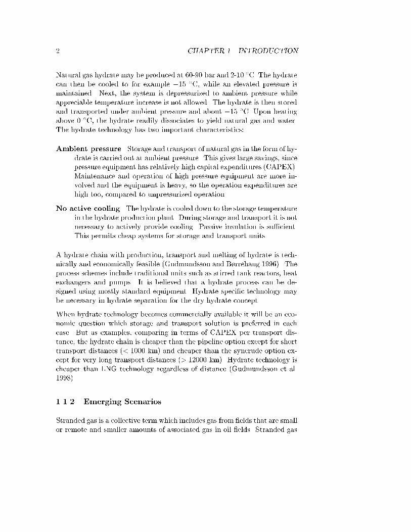
Natural gas hydrate may be produced at 60-90 bar and 2-10 �C. The hydratecan then be cooled to for example �15 �C, while an elevated pressure ismaintained. Next, the system is depressurized to ambient pressure whileappreciable temperature increase is not allowed. The hydrate is then storedand transported under ambient pressure and about �15 �C. Upon heatingabove 0 �C, the hydrate readily dissociates to yield natural gas and water.The hydrate technology has two important characteristics:
Ambient pressure. Storage and transport of natural gas in the form of hy-drate is carried out at ambient pressure. This gives large savings, sincepressure equipment has relatively high capital expenditures (CAPEX).Maintenance and operation of high pressure equipment are more in-volved and the equipment is heavy, so the operation expenditures arehigh too, compared to unpressurized operation.
No active cooling. The hydrate is cooled down to the storage temperaturein the hydrate production plant. During storage and transport it is notnecessary to actively provide cooling. Passive insulation is su�cient.This permits cheap systems for storage and transport units.
A hydrate chain with production, transport and melting of hydrate is tech-nically and economically feasible (Gudmundsson and B�rrehaug 1996). Theprocess schemes include traditional units such as stirred tank reactors, heatexchangers and pumps. It is believed that a hydrate process can be de-signed using mostly standard equipment. Hydrate speci�c technology maybe necessary in hydrate separation for the dry hydrate concept.
When hydrate technology becomes commercially available it will be an eco-nomic question which storage and transport solution is preferred in eachcase. But as examples, comparing in terms of CAPEX per transport dis-tance, the hydrate chain is cheaper than the pipeline option except for shorttransport distances (< 1000 km) and cheaper than the syncrude option ex-cept for very long transport distances (> 12000 km). Hydrate technology ischeaper than LNG technology regardless of distance (Gudmundsson et al.1998).
1.1.2 Emerging Scenarios
Stranded gas is a collective term which includes gas from �elds that are smallor remote and smaller amounts of associated gas in oil �elds. Stranded gas

1.2. TOPICS 3
is expected to play a more important role in the future as focus is puton marginal �elds. E�cient ways to transport this gas to the market willbecome important.
The growing interest in energy sources that are environmentally friendlycompared to fuel oil and coal makes gas attractive. But to develop marginal�elds it is necessary to have cheap and e�ective technical solutions for thestorage and transport. The present work is a contribution in this respect.Focus is put on the fundamental properties of natural gas hydrate.
1.2 Topics
1.2.1 Problem Statements
The major contribution of the present work was construction of laborato-ries and development of experimental techniques. However, these activitiessprung out from some fundamental topics: Thermophysical and composi-tional properties of NGH, such as speci�c heat capacity, heat of dissocia-tion, hydrate number and amount of free water or ice (Chapters 2 and 6).Metastability at ambient pressure and below 0 �C is a thermophysical prop-erty that is treated separately (Chapters 3 and 7). Fractionation, that ishow di�erent components partition between the hydrate phase and the gasphase, is related to the compositional properties and is treated separatelytoo (Chapters 4 and 8).
Thermophysical and compositional properties have to be measured. It isdesirable to correlate thermophysical properties to hydrate composition andin turn to the hydrate production conditions. Developing the method tomeasure thermophysical and compositional properties is a key issue in thepresent work. The starting point was that calorimetry could probably beused, referring to the numerous works by Handa, for example (Handa 1988b).Calorimetric analysis of natural gas hydrate samples that contain a lot offree water (ice) is di�cult. An important task in the present work was todevelop a method to do such analyses.
Metastability as a phenomenon needs to be understood better. The role ofice and how it a�ects metastability is an important issue. It is also necessaryto expand the quantitative knowledge about metastability. It is desirable tomap the metastability region; that is, to correlate the metastable behaviorto storage conditions.

4 CHAPTER 1. INTRODUCTION
Fractionation is not desirable in the hydrate process, but can not be com-pletely avoided (Holder and Manganiello 1982). It is necessary to have morequantitative knowledge about how hydrate production conditions, primarilypressure and temperature, a�ect the fractionation.
Method development is a major challenge in the present work. This in-cludes production, separation, sampling and analysis of hydrate at elevatedpressures. The main challenge was to develop the method to determinethermophysical and compositional properties.
The present work could have relevance for in situ hydrates in permafrostregions and hydrate plugs in pipelines. Permafrost hydrate is subject toconditions that are not very di�erent from storage conditions in the dryhydrate concept. Hydrate plugs may undergo Joule-Thompson cooling toform a mixture of hydrate and ice which resembles the composition of thesamples used in this work.
Dry samples of sII hydrate with ice was used in the present work. Anders-son (1999) studied rheological properties of hydrate slurries. Khokhar (1998)studied storage properties of sH hydrate and reported that hydrate promo-tors act as hydrate stabilizers. It was also found that below 0 �C there isa satisfactory agreement between estimated hydrate dissociation enthalpiesfrom the Clausius-Clapeyron equation and calorimetric measurements.
1.2.2 Scopes of Work
The scopes of the present work were:
� Develop equipment and methods for continuous production and sam-pling of NGH (Sections 5.2 and 6.2).
� Develop a calorimetric method to determine thermophysical proper-ties; enthalpy of dissociation and speci�c heat capacity, and compo-sitional properties; hydrate number and amount of free water (Sec-tion 6.3).
� Develop equipment and methods to quantify metastability propertiesof NGH at di�erent temperatures and compositions of the surroundingatmosphere (Sections 5.5 and 7.2).
� Develop equipment and a method to quantify the e�ect of driving forceon fractionation in NGH formation (Sections 5.6 and 8.2).

Chapter 2
Thermal and Compositional
Properties - Literature Study
This chapter covers hydrate composition and di�erential scanning calorime-try (DSC). It is shown how DSC may be used to determine thermal proper-ties; speci�c enthalpy of hydrate dissociation (�hdiss), hydrate number (n),amount of free water (f) and speci�c heat capacity (cp). Literature mea-surements are reviewed, as are existing models and correlations. Enthalpy ofhydrate dissociation is given broad attention. Composition of the hydratedgas is treated separately in Chapter 4.
2.1 Hydrate Composition
Sloan (1998, Chapter 2) gave a summary of hydrate compositional proper-ties. Hydrates are crystalline solids. The crystal lattice is made of hydrogenbonded water molecules. The water molecules are oriented such that theyform polyhedra, or cages, which share faces. Only a few kinds of cages mayform. These arrange into three di�erent structures known as structure I (sI),structure II (sII) and structure H (sH). sI is built from two di�erent cages.The smallest is made from twelve pentagonals, a 512 cage. The largest ismade from twelve pentagons and two hexagons, a 51262 cage. In a sI unitcell there are two 512 cages and six 51262 cages. sII too is made from twodi�erent cages. The smallest is the 512 cage. The largest is made fromtwelve pentagons and four hexagons, a 51264 cage. In a sII unit cell there
5

6 CHAPTER 2. PROPERTIES - LITERATURE STUDY
are sixteen 512 cages and eight 51264 cages. Cages in sI and sII are illus-trated in Figure 2.1. sI hydrate has 46 water molecules per unit cell while sIIhydrate has 136. sH is made from three di�erent cages. The smallest is the512 cage. The medium sized cage is made from three squares, six pentagonsand three hexagons, a 435663 cage. The largest is made from �ve pentagonsand eight hexagons, a 51268 cage. In a sH unit cell there are three 512 cages,two 435663 cages and two 51268 cages (Sloan 1998).
(b)(a) (c)
Figure 2.1: The di�erent cages in sI and sII hydrate. (a) the 512 cage, (b)the 51262 cage and (c) the 51264 cage (Sloan 1998).
The cages may be empty or contain one guest molecule.1 An empty hy-drate structure with no guest in any of the cages is hypothetical since itwill collapse, or actually never form. A certain portion of the cages mustcontain a guest molecule to stabilize the structure. The guest molecules andthe water molecules interact via van der Waals forces. The guest must benon-polar and small enough to �t into a cage. For sI and sII this limitsthe potential alkane hydrate formers to methane, ethane, propane and iso-butane. Normal-butane is too large, but it may form sH hydrate. Otherhydrate formers are Ar, Kr, N2, O2, Xe, H2S and CO2. sI and sII may formin binary systems (one guest in addition to water). sH is di�erent since itonly forms in ternary (or higher) systems. Examples of sI formers are CH4
and CO2. Examples of sII formers are C3H8 and iso-C4H10. Hydrates withonly one type of guest molecule are called single hydrates. If there are morethan one type of guest the hydrate is called a mixed hydrate. sH is alwaysa mixed hydrate. sI and sII may be mixed or single hydrates.
Because of size di�erences between guests and cages it is not possible forjust any guest to stabilize just any cage. If the diameter of a guest is larger
1There are rare cases with two guests per cage.

2.1. HYDRATE COMPOSITION 7
than the diameter of a cage there is no room for the guest. If the diameterof the guest is less than about a fraction 0.76 of the cage diameter, thenthe attractive forces between the guest molecule and the water molecules inthe lattice are too small to contribute to the stabilization. This applies toHe, H2 and Ne which do not form hydrate. A selection of diameter ratiosis found in Table 2.1. It is seen that methane may enter both cages in sIand the smallest cage in sII. Methane is too small to stabilize the largest sIIcage. Ethane enters the largest cages in both sI and sII. Propane is so largeit can only �t into the largest sII cage, just as iso-butane. Because propaneand iso-butane only �t into the largest sII cage, natural gases will usuallyform sII. Molecules with a diameter less than 0.35 nm are too small to formhydrate. If the diameter is larger than 0.75 nm the molecule is too large.
Table 2.1: Ratios of guest diameter to cage diameter for selected sI and sIIhydrate formers, extracted from Sloan (1998, p. 47). Superscript � indicatesthe cage(s) occupied in simple hydrates.Guest Guest diameter (nm) sI small sI large sII small sII large
CH4 0.436 0.855� 0.744� 0.868 0.655C2H6 0.550 1.08 0.939� 1.10 0.826C3H8 0.628 1.23 1.07 1.25 0.943�
i-C4H10 0.650 1.27 1.11 1.29 0.976�
The hydrate number, n, is de�ned as the ratio of water molecules to gasmolecules in the hydrate, n = nw=ng. If all cages in a hydrate structurewere occupied then the ideal hydrate numbers would result; 534 and 523 forsI and sII, respectively. If all cages in a sII hydrate formed from a natural gaswere occupied, then each volume of hydrate would contain 182 volumes ofgas at standard conditions, 182 Sm3/m3 at 1 bar and 15 �C. But gas hydratesare non-stoichiometric, meaning that not all of the cages are occupied. Inaddition, the fraction of cages that are occupied is system dependent. Itmay well be that 95% of the largest cages are occupied while only 50% ofthe smallest cages are occupied. To calculate the hydrate number from thefractional occupancies, the following equations may be used:
nsI =46
2�s + 6�l(2.1)
nsII =136
16�s + 8�l(2.2)

8 CHAPTER 2. PROPERTIES - LITERATURE STUDY
van der Waals and Platteeuw (1959) developed a statistical thermodynamicmodel of the fractional occupancies of di�erent guests in di�erent cages. Thereduction in chemical potential, ��, when hydrate forms may be expressedas:
�� = �� � �h = �RT (�s ln(1� �s))�RT (�l ln(1� �l)) (2.3)
where �� is the chemical potential of the hypothetical empty lattice and �his the chemical potential of the hydrate with guests at the temperature T .�s and �l are constants equal to the number of small and large cages, respec-tively, per water molecule in the lattice. �s =
16136 = 2
17 and �l =8136 = 1
17for sII hydrate. �s and �l are the fractional occupancies of small and largecages, respectively. According to the model, if �s or �l approaches unity,then the chemical potential reduction becomes in�nite. This is not possi-ble, and consequently a fractional occupancy less than 1 of both cages ispredicted (Holder and Manganiello 1982).
An important question is; what is the smallest hydrate number or the largestfractional cage occupancy that is possible in practical operations? It isshown later (Table 2.3, page 16) that a hydrate number of 5.95 has beenmeasured for sII natural gas hydrate. The fractional cage occupancy is then5.67/5.95=0.953 and the gas content is 173 Sm3/m3. Handa (1986c) pro-duced methane hydrate (sI) and reported a hydrate number of 6.00�0.01.The fractional cage occupancy is then 5.75/6.00=0.958. Handa (1986a) mea-sured hydrate numbers for single hydrates of Kr (n=6.10) and Xn (n=5.90).The ideal hydrate numbers are 5.67 and 5.75 for Kr and Xn, respectively (Sloan1998). The fractional occupancies then become 0.930 for Kr and 0.975 forXn. In these works by Handa, e�orts were made to obtain high cage oc-cupancies. Irrespective of the hydrate former, it seems that a fractionaloccupancy of about 0.95 must be regarded a high value. One way to re-duce the hydrate number and increase the cage occupancy is to produce thehydrate under excess pressure (Handa 1986a).
2.2 Heat Flow DSC
Tian (1923) constructed a calorimeter with two main advantages; high sen-sitivity towards temperature changes (< 10�4 K) and the possibility ofisothermal operation. Calvet and Prat (1963) modi�ed Tian's calorime-ter. Important developments were the ability to do correct measurementof the heat ow without the necessity of stirring and that two calorimetercells were used instead of only one. This made it possible to determine a

2.2. HEAT FLOW DSC 9
di�erential signal, hence the term di�erential scanning calorimetry (DSC).This type of calorimeter is often called a Tian-Calvet heat ow calorimeterand is illustrated in Figure 2.2.
��������
��������
������������
��������
������������
��������
����������������
������������
��������
��������
��������
����
����
������
����
��������
������������
������
����
Container for sample cell
S R
Insulation
Nitrogencooling
Thermostat
Thermalblock
Heat flowsensors
Container for reference cell
Figure 2.2: Sketch with the main items of a Tian-Calvet heat ow calorime-ter (not to scale).
The two cells are placed in a thermal block. One of the cells is the samplecell. The other is the reference cell, which may contain a reference sample orbe empty. Both cells are surrounded by up to 1000 heat ow sensors. Theheat ow signal for both cells are registered. The output heat ow is thedi�erence between the signals of the two cells, hence the term di�erential.The cells are thermally decoupled, i.e. heat is only transfered between a celland the thermal block - there is no heat ow from one cell to the other. Forcalorimeters with cylinder type cells (disc type is also available) the samplevolume is relatively large, which may be an advantage. But the thermalinteria is large too and quick heating or cooling is not possible.
It is impossible to make two identical cells, so a portion of the total signal isdue to the di�erence between the cells. This portion may be relatively smalland ignored, or it may be corrected by subtracting the signal of a blankrun, where both cells were empty. This type of correction is relevant forvery precise measurements, like when the signal from the reacting system isweak (H�ohne et al. 1996).

10 CHAPTER 2. PROPERTIES - LITERATURE STUDY
A DSC curve (thermogram) typically has the heat ow, _Q (W), on theordinate and time on the abscissa. Temperature may be plotted along asecondary ordinate axis or on the abscissa instead of time, see Figure 2.3.The di�erential heat ow is proportional to the temperature di�erence, �T ,between the sample cell end the reference cell:
_Q = K�T (2.4)
whereK is a calibration constant. The area of a peak is the area between thebase line and the heat ow signal. The area, Q (J), is found by integrating_Q over time:
Q =
Z_Qdt = K
Z�T dt (2.5)
The baseline is not measured in the peak range. Thus, to integrate a peak,the baseline has to be interpolated over the temperature or time intervalcovered by the peak. The interpolated baseline is the line which in therange of a peak is constructed such that it connects the measured curvebefore and after the peak as if there was no peak. This is illustrated inFigure 2.3. It is desirable that the interpolated baseline accounts for anychange in the heat capacity on the temperature interval of interest. It isnot obvious how this can be done, but for a change of the baseline betweeninitial and �nal temperatures Ti and Tf , respectively, a good approximationof the interpolated baseline, _Qbl, is to assume that
_Qbl = (1� �) _Qiex + � _Qfex (2.6)
where � is the degree of reaction or transition. _Qiex and _Qfex are the seg-ments of the measured curve extrapolated into the peak range from the ini-tial (i) and �nal (f) end, respectively. _Qiex and _Qfex need to be expressed aspolynomials and these polynomials extrapolated into the peak range. The_Q slopes in the points Ti and Tf should not di�er very much (H�ohne et al.1996).
The enthalpy is equal to the (accumulated) heat for a process at constantpressure; �H = Q. Speci�c enthalpy, �h (J/mol), of a peak is found bydividing the total enthalpy change, �H (J), by the amount of substance, n(mol), thus �h = �H
n . Mass basis could also be used.

2.2. HEAT FLOW DSC 11
T i T f
Hea
Interpolated baseline
t
flow
Temperature
f,exQ
.Q
i,ex
.α=1α=0
Base line
Peak
Figure 2.3: Construction of the baseline in the peak region (H�ohne et al.1996). � is the degree of reaction of conversion.
The speci�c heat capacity at constant pressure, cp (J/gK), may be deter-mined by calorimetry in di�erent ways. The classical procedure is to heatthe sample at a constant rate over the temperature interval of interest. Theresulting curve is corrected by subtracting a blank run. It is then possibleto express the corrected enthalpy change, �H (J), by a best �t expression.By de�nition, cp is the derivative with respect to temperature of this �ttedexpression when referred to the amount of sample. On mole basis (H�ohneet al. 1996):
cp =d�H
ndT=d�h
dT(2.7)

12 CHAPTER 2. PROPERTIES - LITERATURE STUDY
2.3 Dissociation Enthalpy, Hydrate Number and
Free Water Measurements by Calorimetry
The dissociation of hydrate may follow two schemes:
G � nH2O(h) = nH2O(s) +G(g) for T < 273:15 K
or
G � nH2O(h) = nH2O(l) +G(g) for T > 273:15 K
where G is the guest gas. In addition the hydrate may contain free water(ice) which melts:
H2O(s) = H2O(l)
The di�erence in enthalpy between the two �rst reactions is assumed to bethe enthalpy of ice melting (Handa 1986a). After dissociation, there is alsothe possibility of gas desorption;
G(aq) = G(g)
The enthalpy of desorption does not contribute to the dissociation enthalpy.But it may become important when measuring apparent or overall enthalpiesof consecutive processes.
Calorimetric methods are used to measure the speci�c enthalpy of hydratedissociation, �hdiss, in units J/mol or J/g. Such measurements are inti-mately related to the hydrate number (n) and the amount of free water(f) through the mass and energy balances. The measurements are di�cult,since the hydrate system is reactive and since it is di�cult to make hydratesamples which do not contain any free water. Still, there have been madea number of measurements on single hydrates. Few data are available formixed hydrates, such as natural gas hydrate, and no reliable measurementsof the standard enthalpy of natural gas hydrate dissociation, �h�diss, werefound. This is an important motivation for the present work.
The �hdiss units may seem ambiguous. To clarify, in the unit J/mol, \mol"refers to a base of 1 mol hydrate with the unit formula G � nH2O. Thus, asystem which contains m moles of hydrate also contains m moles of hydratedgas. The molar mass of the hydrate is MG + 18n where MG is the molarmass of the guest, n is the hydrate number, and 18 is the molar mass ofwater. In the unit J/g, \g" refers to a base of 1 g hydrate.

2.3. MEASUREMENTS BY CALORIMETRY 13
2.3.1 Measurements by Handa et al. (�h�diss, n and f)
Calorimetry Procedure
Handa et al. (1984) and Handa (1986a) described a Tian-Calvet heat owcalorimeter which was modi�ed such that the sample could be pressurizedwith gas, see Figure 2.4. A calorimetric procedure was given to �nd h�diss,n and f for single hydrates from xenon and krypton with 1 to 8 %mass offree water (ice). Two runs are necessary.
Calorimeter
11
910
4
5
3
7
2
1
S R
8 6
To vacuum
Figure 2.4: Block diagram of Handa's calorimeter (Handa 1986a). S andR: sample and reference cells. 1, 2, 3, 4 and 5: high-pressure high-vacuumvalves. 6: High-pressure high-vacuum quick-connect-disconnect coupling.7 and 8: Pressure transducers. 9: Gas cylinder. 10: Expansion chamber.11: Thermometer.
In the �rst run the sample is heated from 270 K to about 275 K at a rateof 8.3�10�4 K/s (0.05 K/min). The pressure is equal to the equilibriumpressure at about 277 K. The purpose is to melt any ice in the sample, todetermine the amount of free water. Valve 3 is open and 2 is closed.
To prepare for the second run, the temperature is brought down to 78 K andthe pressure reduced to less than 1 kPa. Valves 3 and 5 in Figure 2.4are left open. The sample is then heated at a scanning rate of 2.8�10�3 K/s(0.168 K/min) to 290 K while recording the system pressure and the tem-

14 CHAPTER 2. PROPERTIES - LITERATURE STUDY
perature in the expansion chamber (10). The purpose is to dissociate thehydrate. The large volume of the expansion chamber causes the pressureto stay low. This ensures smooth dissociation. When all of the hydrate isdissociated the pressure is usually between 80 and 100 kPa (Handa 1986a).
Raw Data Processing
The amount of hydrated gas, ng, is calculated from PV T data obtainedduring the second run:
ng =(Pf � Pi � Pw)(Vtot � Vw)
RTg +B(Pf � Pi � Pw)(2.8)
where Pf is the pressure at the end of the second run and Pi is the pressurejust before dissociation started. Pw is the water saturation vapor pressureat the cell temperature Tc at the end of the second run. Vtot is the totalsystem volume and Vw is the volume of liquid water in cell S (found byweighing as the water density is known). B is the second virial coe�cientof the gas (Dymond and Smith 1980). Tg is the volume-weighted averagetemperature of the gas,
Tg =V1Tr + 0:5V2(Tc + Tr) + Tc(VS � Vw)
Vtot � Vw(2.9)
where V1 is the volume enclosed by valves 1, 2, 3 and 4 with 5 open.Tr is the room temperature. The volume V2 is enclosed by 3 and the topof the sample cell (S). The temperature of the gas in V2 was assumed to bethe average of the cell temperature, Tc, and the room temperature, Tr. VSis the volume of the sample cell. The e�ect on ng because of gas absorbedby the water is negligible for Kr hydrate with 2-8 %mass ice and Xn hydratewith 1 %mass ice.
The amount of hydrate water, nw, is found by subtracting the amount offree water, nw;ice, found in the �rst run, from the total amount of water,nw;tot, found by weighing after the second run:
nw = nw;tot � nw;ice (2.10)

2.3. MEASUREMENTS BY CALORIMETRY 15
The hydrate number is then calculated using:
n =nwng
(2.11)
Results
Results from �hdiss and n measurements are collected in Table A.1. A se-lection of the more recent and reliable data at standard conditions (�h�diss)are given in Table 2.2. The measurements are accurate to about �1%.
It is seen how the dissociation enthalpy is substantially higher for tempera-tures above 275.15 K than below this temperature. The explanation is thatabove 273.15 K the hydrate dissociates into gas and liquid water, while be-low it dissociates into gas and ice. Additional heat is required to form liquidwater instead of ice.
Table 2.2: Standard (P=101,325 Pa) enthalpies of hydrate dissocia-tion, �h�diss. The natural gas hydrate labeled NGH8 contained (%mol):methane (99.93), ethane (0.01), propane (0.01), iso-butane (0.05) and wasretrieved during the Deep Star Drilling Project. Sample NGH9 was re-trieved from the Gulf of Mexico and its �h�diss is only an estimate sincethe composition of the hydrate could not be determined precisely (Handa1988b).
Guest �h�diss n T Remark ReferencekJ/mol - K
sI NGH8 17.50 CH4�5.91H2O 273 h!i+g (Handa 1988b)
sII NGH9 27.8-33.1 0-20 %mass ice 220-260 h!i+g (Handa 1988b)
CH4 18.13�0.27 6.00�0.01 160-210 h!i+g (Handa 1986c)
C2H6 25.70�0.37 7.67�0.02 190-250 h!i+g (Handa 1986c)
C3H8 27.00�0.33 17.0�0.1 210-260 h!i+g (Handa 1986c)
i-C4H10 31.07�0.20 17 assumed 273.15 h!i+g (Handa 1988a)
CH4 54.19�0.28 6.00�0.01 273.15 h!w+g (Handa 1986c)
C2H6 71.80�0.38 7.67�0.02 273.15 h!w+g (Handa 1986c)
C3H8 129.2�0.4 17.0�0.1 273.15 h!w+g (Handa 1986c)
i-C4H10 133.2 17 assumed 273.15 h!w+g (Handa 1988a)

16 CHAPTER 2. PROPERTIES - LITERATURE STUDY
2.3.2 Other Measurements (�hdiss)
Maksimov (1996) reviewed a number of Russian publications and summa-rized works by Groisman (1985), Groisman and Savvin (1988) and Cherskyet al. (1982). They made an adiabatic casing in which a measurement cellwith constant heat supply was placed. �hdiss were measured for sII NGHsamples in the pressure range 1.1 to 14 MPa. The �hdiss values are in therange 500 to 540 J/g for n in the range 5.95 to 6.7. In the present work thesedata were converted to cover the range 68.8 to 77.3 kJ/mol, see Table 2.3.
Table 2.3: Enthalpies of hydrate dissociation, �hdiss, reproduced from Mak-simov (1996). The data were originally published by Chersky et al. (1982)and Groisman (1985) at pressures of 1.1-14 MPa, i.e. not standard state,for the transition h!w+g. The composition of the samples are given inTable A.2.
Sample �hdiss(kJ/mol) n P (MPa) T (K)
sII NGH1 77.3 6.7 1.1 273sII NGH2 72.5 6.6 2.2 278sII NGH3 72.1 6.3 4.1 283sII NGH4 73.9 6.2 5.9 286sII NGH5 70.9 6.1 7.6 288sII NGH6 71.4 6.1 8.5 289sII NGH7 68.8 5.95 14.0 293
Kobayashi and Lievois (1988) built a Tian-Calvet heat ow calorimeterwhich was specially designed to study hydrate. The cells were large, 1.158 dm3.The cells featured magnetic stirrers. Methane hydrate was formed in thesample cell by operating it as a stirred batch reactor. Having formed a su�-cient amount of hydrate the system was left to equilibrate for the base line toestablish. The obtained value for the speci�c enthalpy of methane hydratedissociation to gas and water at 278 K and 4.34 MPa (close to equilibrium)was �hdiss=13,090 cal/gmoleCH4 . In SI units: �hdiss=54.769 kJ/mol. Thehydrate number was about 6.0, so the values transform into 441.7 J/g.
Rue� et al. (1988) also used DSC technique to determine �hdiss of methanehydrate. For six di�erent samples �hdiss varied between 421.23 and 436.66 J/gwith n=6.15. They also measured cp for methane hydrate.

2.4. DISSOCIATION ENTHALPY MODELS AND CORRELATIONS 17
2.3.3 Non-calorimetric Techniques to Measure n
With Raman spectroscopy, n can be measured and it is possible to determinehow the guests partition between the di�erent cages. This can not be done bycalorimetry. Sum et al. (1996) were the �rst to use Raman spectroscopy onhydrates of natural gas components. Among the systems studied were CH4,C3H8 and CD4+C3H8. The measurements compared well to predictionsfrom the statistical thermodynamic model of van der Waals and Platteeuw(1959). For methane hydrate, Sum et al. found that the hydrate numberincreases if pressure and temperature increase. It should also be noted thatRaman spectroscopy may be used to quantify the content of gas in the freewater under hydrate forming conditions or at equilibrium.
Uchida et al. (1999) analyzed naturally occurring hydrate (CH4 > 99 %mol)from Blake Ridge (leg 164) and synthetic methane hydrate. They concludedthat the hydrate number is constant at about 6:2 � 0:2 (nideal = 5:75).It does not change as a function of formation conditions (P=3.0-8.1 MPa,T=273.2-278.4 K) or depend on the amount of free water. This is a di�erentconclusion than Sum et al. (1996) reached. The large cage was occupied toa fraction of 0.976-0.981 and the small to a fraction of 0.715-0.857.
Ripmeester et al. (1988) demonstrated that 13C NMR can be used to mea-sure n. The original paper and the summary by Sloan (1998, pp. 310-312)are referred to for the details.
2.4 Dissociation Enthalpy Models and Correlations
The Clausius-Clapeyron equation is the most widely used model to calcu-late enthalpy of hydrate dissociation, �hdiss. Handa (1988b) points thisout, although he refers to the Clapeyron equation - an example that the ter-minology is somewhat loose. The Clausius-Clapeyron equation is treated inSection 2.4.1. Models that represent alternatives to the Clausius-Clapeyronequation are treated in Sections 2.4.2 to 2.4.4.
2.4.1 The Clausius-Clapeyron Equation
By equating Gibbs free energies, GA(P; T ) = GB(P; T ), and combining basicthermodynamic relations, the Clapeyron equation is derived:

18 CHAPTER 2. PROPERTIES - LITERATURE STUDY
dPsaturationdT
=�hABT�vAB
=�sAB�vAB
(2.12)
for the equilibrium between two phases A and B of a pure substance (Barrow1979). h, v and s are the molar enthalpy, volume and entropy, respectively.The equation expresses the P -T relation along a phase transition line for apure substance. The Clapeyron equation is exact and applies to liquid-gas,solid- uid and solid-solid phase equilibria.
For liquid-gas equilibria at low pressures the Clapeyron equation simpli�esto the Clausius-Clapeyron equation where P is the saturation pressure:
d lnP
d 1T
=��hvap
R(2.13)
which upon integration and rearrangement yields:
lnP =��hvap
R�1
T+ C (2.14)
P is the vapor pressure of a pure liquid, �hvap is the speci�c enthalpy ofvaporization and C an integration constant. Plotting lnP as a function of1=T yields a straight line. The enthalpy of vaporization is determined bythe slope of the line, a:
a ��lnP
� 1T
=��hvap
R(2.15)
thus the heat of vaporization is:
�hvap = �aR (2.16)
The Clausius-Clapeyron equation is not exact, but is based on two assump-tions: vgas � videalgas and vliquid � vgas where v indicates molal volumes ofthe di�erent phases.
The Clausius-Clapeyron equation has been extended from one componentvapor-liquid systems into hydrate systems. The model is widely referred toin hydrate papers, for instance by Fleyfel and Sloan (1991), Groisman and

2.4. DISSOCIATION ENTHALPY MODELS AND CORRELATIONS 19
Savvin (1988) and Parent (1948). The equation enables the calculation of theheat of hydrate dissociation, as the hydrate dissociation process is assumedanalogous to liquid vaporization. Accordingly, the enthalpy of vaporizationis replaced by the enthalpy of dissociation, �hdiss. To account for non-idealgas behavior, the original equation is modi�ed by the introduction of thecompressibility factor, z:
�hdiss = �zaR (2.17)
An underlying assumption is that �hdiss is independent of temperature.�hdiss is not a very strong function of the temperature, so for narrow tem-perature intervals the assumption is reasonable. Correlations that accountfor temperature dependency are given in Section 2.4.4. Comparison be-tween calculated �hdiss values and calorimetry measurements has proven theClausius-Clapeyronmethod accurate within 1-5% for hydrates of some singleguests; methane, ethane, propane and iso-butane. The Clausius-Clapeyronequation has been discussed in the literature and agreement has been reachedthat the Clausius-Clapeyron equation is only valid for univariant systemslike Hydrate *) Water + Gas and with three restrictions (Sloan and Fleyfel1992):
� The fractional occupancy of each cage is about constant.
� The volume change of the condensed phase is negligible compared tothe gas volume.
� The gas consumption is about constant.
Handa (1986a) states that in general the Clapeyron equation results in largeerrors. One reason is the poor quality of most dissociation pressures reportedin the literature. Such errors propagate through calculations to result incorrespondingly large errors in values of dissociation enthalpy. As a result,many of the �hdiss values reported in the literature are questionable. On theother hand, Maksimov (1996) refers to the works by Chersky et al. (1982)and Groisman (1985) and points out that the di�erence between Clausius-Clapeyron estimates and measured �hdiss values for sII natural gas hydratedoes not exceed 3%. This is acceptable for engineering applications.

20 CHAPTER 2. PROPERTIES - LITERATURE STUDY
When doing Clausius-Clapeyron calculations, one has to assess a value tothe independent variable z. Should it be desirable to take pressure and tem-perature e�ects on z into account, this rises a separate modeling question.The standard procedure is to determine z(P; T ) by solving a cubic equationof state. Rue� et al. (1988) in a paper on hydrate dissociation refer tothe Peng-Robinson equation of state. To calculate dissociation enthalpies atstandard conditions it will usually be a good approximation to assume thatz = 1. The step-by-step procedure for Clausius-Clapeyron calculations are:
1. Perform hydrate dissociation experiments to record the equilibriumpressures, at di�erent temperatures.
2. Plot the pressure-temperature pairs in a coordinate system with lnPon the ordinate axis and 1
T on the abscissa axis.
3. Calculate the slope, a.
4. Assess a value to z.
5. The enthalpy of dissociation is now: �hdiss = �zaR.
Khokhar (1998) used the Clausius-Clapeyron equation to calculate �hdissbelow 273.15 K for hydrates of di�erent compositions and for di�erent struc-tures. Among di�erent sII hydrates, he found that �hdiss does not vary alot even if the composition varies, see Table 2.4. The implication is that�hdiss is about the same for a wide range of gas compositions. The mix-tures methane + propane and methane + n-butane can be said to representnatural gases. The average �hdiss below 273.15 K for the correspondinghydrates were 27.85 kJ/mol. 27.8-33.1 kJ/mol was the �hdiss interval mea-sured2 by Handa (1988b) on a naturally occurring sample of sII natural gashydrate. The correspondence is good.
2.4.2 Guest Size Dependent Enthalpy Estimation
Sloan and Fleyfel (1992) suggested that to an approximation, �hdiss is deter-mined by the type of cage occupied, which in turn is determined by the sizeof the guest(s). �hdiss is independent of the guest type - only the size of the
2This was for measurements on the sample referred to as NGH9 in Table 2.2. A uniquevalue could not be found and the interval is based on assumptions of no ice in the sample(27.8 kJ/mol) and 20 %mass ice (33.1 kJ/mol).

2.4. DISSOCIATION ENTHALPY MODELS AND CORRELATIONS 21
Table 2.4: Clausius-Clapeyron calculations below 273 K for di�erent sIIhydrates (Khokhar 1998).
Guest(s) Slope (1/K) �hdiss (kJ/mol)
Propane �3583:62 28.96i-Butane �3544:45 28.64Methane + propane �3361:48 27.53Methane + n-butane �3533:02 28.17
guest matters. To support the hypothesis a number of Clausius-Clapeyronplots were presented for single and mixed hydrates. The overall observationwas that hydrates of the same structure and with the same types of cagesoccupied had about the same �hdiss.
For example, single hydrates of propane and iso-butane are sII hydratesand only the largest cavities are occupied. The slope in Clausius-Clapeyronplots are �15100 K and �15700 K for propane and iso-butane, respectively.The di�erence is about 4%. Double sII hydrates with both cages occupiedshow the same resemblance. For example, a mixture of 1 %mol propane inmethane and a mixture of 36.2 %mol propane in methane have the sameslopes (within the experimental error); �9802 K. The overall results arepresented in Table 2.5.
The size dependent model was disputed by Skovborg and Rasmussen (1993)who claimed that the grouping of components according to Sloan and Fleyfelis not possible. For example it was pointed out that the slope, and thus�hdiss, depends on the hydrate number. For the slope to be constant, z toomust be constant over the pressure and temperature range of interest.
Table 2.5: The guest size dependent model for �hdiss prediction above273 K by Sloan and Fleyfel (1992). It assumes that for a given structure(sI or sII) �hdiss is determined by which cages are empty (e) and which areoccupied (o).
Structure Large Small � �hdiss (kJ/mol)
sI o o 54-57sI o e 71-74sII o o 79sII o e 126-130

22 CHAPTER 2. PROPERTIES - LITERATURE STUDY
2.4.3 Chemical Potential Model
Handa (1986a) derived a model for �hdiss as follows:
For the 3-phase (h-l-g) equilibrium at T and P we have:
�h = n�w + �g (2.18)
where � is the chemical potential of hydrate (h), liquid water (w) and hy-drate former (g). n is the hydrate number. Pure solid, pure liquid and pureideal gas at 273.15 K and 101,325 Pa were taken as standard states for solid,liquid and gas, respectively. This yields:
�h = ��h +
Z P
P �
vhdP (2.19)
�w = ��w +
Z P
P �
vwdP +RT lnaw (2.20)
�g = ��g +RT ln
f
f�(2.21)
where superscript � refers to the standard state, (101,325 Pa), vh is themolar volume of hydrate, vw is the partial molar volume of water, aw is theactivity of water and f is the equilibrium fugacity of the hydrate forminggas. n is a function of P leading to the assumption that the hydrate in itsstandard state has a hydrate number as it would have at P .
When the gas solubility in the water is low, lnaw � �xg and vw � v�w wheresuperscript � denotes pure. The e�ect of P on the volumetric properties ofthe condensed phases is assumed neglectible, yielding the model equation:
��� = �nxgRT +RT lnf
f�+ (P � P �)(n�
w � vh) (2.22)
where
��� = ��h � n��
w � ��g (2.23)

2.4. DISSOCIATION ENTHALPY MODELS AND CORRELATIONS 23
For the (h-i-g) equilibrium, the standard state functions are obtained fromthe model equation by introducing xg = 0 and v�w = vice. It is indicatedhow the chemical potential model may be developed further and used to�nd h�diss.
Compared to the Clausius-Clapeyron equation, Handa's model is di�cult touse and there is nothing to gain regarding accuracy, which is about �5%.The chemical potential model is not persuied further in the present work.
2.4.4 Correlations
Holder et al. (1988) wrote a comprehensive review on phase behaviour insystems containing clathrate hydrates. An empirical correlation was pro-posed for �hdiss (J/mol). The correlation includes constants c and d fordi�erent guests and temperature intervals. The constants are given in Ta-ble 2.6. Note that the correlation yields the dissociation enthalpy at theequilibrium pressure and not at standard pressure.
�hdiss = 4:18(c + dT ) (2.24)
Table 2.6: Coe�cients for calculating �hdiss according to the correlation�hdiss = 4:18(c + dT ) (Holder et al. 1988).
Gas Structure c d T range (K)
CH4 I 6,530 �12:0 248-27313,500 �4:0 273-298
C2H6 I 8,460 �9:6 248-27313,300 15.0 273-287
C3H8 II 7,600 �4:9 248-27337,750 �250:1 273-278
CO2 I 9,290 �12:9 248-27319,200 �15:0 273-284
N2 I 493,400 �9:0 248-2736,190 18.4 273-298
H2S I 8,490 �7:8 248-2736,780 31.5 273-298

24 CHAPTER 2. PROPERTIES - LITERATURE STUDY
Based on the Clausius-Clapeyron equation, Selim and Sloan (1990) gavecorrelations to calculate �hdiss for natural gas hydrate in sediment, belowand above 273 K. The correlations have the same form as the one by Holderet al. (1988).
�hdiss = 215:59 � 103 � 394:945T (J/kg) for T = 248-273 K�hdiss = 446:12 � 103 � 132:638T (J/kg) for T = 273-298 K
Zakrzewski and Handa (1993) studied dissociation of tetrahydrofuran hy-drate in con�ned geometries. The enthalpy of hydrate dissociation was sup-pressed as much as 36.9% compared to bulk dissociation. This demonstratesthat �hdiss correlations for sediment hydrate, as the one by Selim and Sloan(1990), may not apply to bulk hydrate. On the other hand, these partic-ular correlations are based on Clausius-Clapeyron calculations (\modi�edClapeyron equation"), which do apply to bulk hydrate.
2.4.5 Dissociation Enthalpy Comparison
A number of dissociation enthalpy measurements and have now been re-ferred, along with di�erent ways to predict such values. Now, the di�erentvalues are compared for two cases; methane and natural gas.
Methane
Figure 2.5 shows �ve di�erent dissociation enthalpies, labeled a-e, for methane.Clausius-Clapeyron calculations overestimate the experimental values byabout 4%. The guest size dependent model by Sloan and Fleyfel (1992)shows a aimilar overestimate. This is not unexpected since the model isjusti�ed by a number of Clausius-Clapeyron calculations. The correlationby Holder et al. (1988) underestimates by about 5%.
Natural Gas
Figure 2.6 shows three di�erent Clausius-Clapeyron lines. They are basedon the Mastahskoe gas composition given is Section 2.5.2. The data pointsreproduced from Maksimov (1996) are near-equilibrium velues of pressureand temperature. The other two lines are based on qeuilibrium simulationsusing CSMHYD and PVTsim.

2.4. DISSOCIATION ENTHALPY MODELS AND CORRELATIONS 25
0
10
20
30
40
50
60
a b c d e
∆ hd
iss [
kJ/
mol
]
correlation
calori
metry
calori
metry
Clausius Clapeyron
guest size
model
Figure 2.5: Comparison of measurements (col. b,c) and predictions, of en-thalpy of methane hydrate dissociation. a: Correlation by Holder et al.(1988), b: Calorimetric measurement by Handa (1986c), c: Calorimetricmeasurement by Kobayashi and Lievois (1988), d: Clausius-Clapeyron cal-culation by Sloan and Fleyfel (1992), e: Guest size dependent model by Sloanand Fleyfel (1992).
Figure 2.7 shows enthalpies of natural gas hydrate dissociation from theClausius-Clapeyron calculations, and enthalpies according to the guest sizedependent model by Sloan and Fleyfel (1992) and the correlation by Selimand Sloan (1990). The guest size dependent model gives about the samevalue as Clausius-Clapeyron calculations. The Clausius-Clapeyron calcula-tions overestimate the calorimetric measurments between 5% and 17%. Sim-ilar deviations were seen for methane, but the deviation between Clausius-Clapeyron calculations and measurements are larger for natural gas than formethane. The correlation by Selim and Sloan (1990) deviate �18% from theexperimental value. This is corresponding to the observation by Zakrzewskiand Handa (1993) who found that the correlation signi�cantly underesti-mates enthalpies of bulk dissociation.

26 CHAPTER 2. PROPERTIES - LITERATURE STUDY
Maksimov (1996)lnP = -10167/T + 37.345∆hdiss = -zaR ~ -1(-10167)8.314 J/mol = 84.5 kJ/mol
CSMHYDlnP = -9179.2/T + 33.579Dhdiss = -zaR ~ -1(-9179.2)8.314 J/mol = 76.3 kJ/mol
PVTsimlnP = -9517.2/T + 34.718Dhdiss = -zaR ~ -1(-9517.2)8.314 J/mol = 79.1 kJ/mol
-0.2
0
0.2
0.4
0.6
0.8
1
1.2
1.4
1.6
0.00352 0.00354 0.00356 0.00358 0.0036 0.00362 0.00364 0.00366 0.003681/T [1/K]
lnP
[-]
Figure 2.6: Clausius-Clapeyron plot of Mastahskoe gas. Maksimov (1996)provided experimental P and T values, while those obtained by CSMHYDand PVTsim are equilibrium simulations based on the gas composition.
2.5 Speci�c Heat Capacity
2.5.1 Measurements
To determine cp of Kr and Xn hydrates, Handa (1986a) used the classicalmethod described in Section 2.2. The measurements were corrected by sub-tracting the signal of a blank run. Heat capacity for hydrate was obtainedby correcting for any ice in the sample while it was assumed that the heatcapacities of hydrate and ice were additive. cp for hydrate are given in unitsof J/molK where mol refers to the hydrated gas. Selected results for tem-peratures not too far below 273 K are given in Table 2.7. Groisman (1985)measured cp of natural gas hydrate, and reported values of 2.14-2.88 J/gKfor temperatures of 213-275 K.

2.5. SPECIFIC HEAT CAPACITY 27
0
10
20
30
40
50
60
70
80
90
a b c d e f
∆ hd
iss [
kJ/
mol
]
correlation
Claus Clap CSMHYD
guest size
model
Claus Clap PVTsi
m
Claus Clap real data
calori
metry
Figure 2.7: Comparison of measurements (col. b) and predictions, of en-thalpy of Mastahskoe gas hydrate dissociation. a: Correlation by Selimand Sloan (1990), b: Calorimetric measurements reproduced from Maksi-mov (1996), c: Clausius-Clapeyron calculation from CSMHYD equilibriumsimulations, d: Guest size dependent model by Sloan and Fleyfel (1992),e: Clausius-Clapeyron calculation from PVTsim equilibrium simulations andf: Clausius-Clapeyron calculation from experimental data taken from Mak-simov (1996).
2.5.2 Models and Correlations
Maksimov (1996) reviewed Russian works. With reference to Groisman(1985) the following model was given with unit J/gK:
cp;NGH =4:5R + 18n(2:3 + 8:4732 � 10�3(T � 273:15))
MNG + 18n(2.25)
where R is the universal gas constant, n is the hydrate number, T is abso-lute temperature and MNG is the molecular mass of the hydrated naturalgas. A comparison of measurements and model calculations showed an errorof �5%.

28 CHAPTER 2. PROPERTIES - LITERATURE STUDY
Table 2.7: Selected measured values of cp for single hydrates.
Guest cp (J/molK) n T (K) Reference
CH4 233.7 6.00 240 (Handa 1986c)CH4 257.6 6.00 270 (Handa 1986c)C2H6 310.9 7.67 240 (Handa 1986c)C2H6 337.8 7.67 260 (Handa 1986c)C3H8 644.0 17.0 240 (Handa 1986c)C3H8 710.2 17.0 260 (Handa 1986c)Kr 217.9 6.10 240 (Handa 1986a)Kr 243.3 6.10 270 (Handa 1986a)Xn 218.8 5.90 240 (Handa 1986a)Xn 242.4 5.90 270 (Handa 1986a)
The measurements were made on synthetic hydrate made from natural gasproduced at the Mastahskoe �eld in Yakutia. The composition was (%mol):CH4 (91.509), C2H6 (3.942), C3H8 (1.220), i-C4H10 (0.454), n-C4H10 (0.140),i-C5H12 (0.147), n-C5H12 (0.051), H2 (2.0) and O2 (0.4). This yielded anaverage molecular mass of 17.63 g/mol. The composition of the hydrate wasnot speci�ed.
Maksimov (1996) with reference to the original work by Istomin and Yaku-shev (1992) assumed that cp of gas hydrates may be modeled in terms ofadditive contributions from the lattice and the guest(s). cp (J/molK) ofthe empty lattices of Xe and Kr compare well to cp of ice Ih in the range240-270 K. The di�erence is about �4%.
The following model was proposed to calculate cp (J/molK):
cp = nc� +Xi
cixi (2.26)
where c� is the heat capacity of the empty lattice (c� � ciceIh), ci is the molarheat capacity of the hydrated gas of type i which is present to a fraction xiin the hydrated gas. cp may be converted from J/molK to J/gK by dividingthe cp value from Equation 2.26 by (MG + 18n). Empirical cp correlationsfor single hydrates are given in Table 2.8. The error is about �1%.

2.6. THERMAL CONDUCTIVITY AND EXPANSIVITY 29
Table 2.8: Empirical correlations of speci�c heat capacity for single hydrates.cp correlation (J/molK) T (K) Reference
cp(CH4�6:00H2O)=6:6 + 1:4538T � 0:3640 � 10�2T2 + 0:6312 � 10�5T3 85-270 (Handa 1986c)
cp(C2H6 � 7:67H2O)=22:7 + 1:8717T � 0:5358 � 10�2T2 + 1:076 � 10�5T3 85-265 (Handa 1986c)
cp(C3H10 � 17:0H2O)=�37:6 + 4:8606T � 1:625 � 10�2T2 + 3:291 � 10�5T3 85-265 (Handa 1986c)
cp(Xe�5:90H2O)=2:12 + 1:3516T � 3:232 � 10�3T2 + 5:622 � 10�6T3 85-270 (Handa 1986a)
cp(Xe�6:29H2O)=36:0 + 0:77505T 150-230 (Handa 1986b)
cp(Kr�6:10H2O)=�4:76 + 1:4345T � 3:398 � 10�3T2 + 5:391 � 10�6T3 85-270 (Handa 1986a)
2.6 Thermal Conductivity and Expansivity
Sloan (1998) and Maksimov (1996) reviewed measurements of thermal con-ductivity, �, for hydrate. Not much seems to be reported. Two methodsare in use; the transient method and the steady state method. Accuraciesrange between 8 and 12%. Data are given in Table 2.9.
Table 2.9: Collection of experimental data for thermal conductivity (�) forclathrate hydrates. The reference by Istomin and Yakushev (1992) refers toother original publications of the data.Guest/structure � (W/Km) T (K) Reference
Ice 2.23 263 (Sloan 1998, p. 60)sI 0.49�0:2 263 (Sloan 1998, p. 60)sII 0.51�0:2 263 (Sloan 1998, p. 60)Methane 0.45 216.2 (Cook and Leaist 1983)Methane 0.393 275.15 (Stoll and Bryan 1979)Methane 0.45 213 (Istomin and Yakushev 1992)Propane 0.39 275.15 (Stoll and Bryan 1979)Xenon 0.36 245 (Handa and Cook 1987)Ethylenoxide 0.49 263 (Istomin and Yakushev 1992)Tetrahydrofuran 0.51 260 (Istomin and Yakushev 1992)1,3-dioxane 0.51 260 (Istomin and Yakushev 1992)
Groisman (1985) studied the thermal conductivity for NGH from a gas mix-ture containing C1 to C5 alkanes, hydrogen and oxygen. Average molecularmass of the gas was 17.63 g/mol (gravity 0.61). It was found that �NGH
increases with temperature in the range 223 to 275 K and with pressurein the range 2.1 to 10.0 MPa. Pressure dependancy was weak. �NGH wasmainly determined by the density in the range 300 to 700 kg/m3.

30 CHAPTER 2. PROPERTIES - LITERATURE STUDY
The thermal conductivity of hydrate is conciderably lower than that of ice.This di�erence can be used to quantify the amount of hydrate in a hydrate-ice sample (Sloan 1998).
Much research remains regarding hydrate thermal conductivity. But it isindicated that neither the type of guest molecule nor the structure type haveappreciable e�ect on the thermal conductivity. Groisman (1985) arrivedat an empirical ralation between NGH thermal conductivity (W/mK) anddensities in the range 300 to 700 kg/m3:
�NGH = �0:21 + 8:33 � 10�4�NGH (2.27)
Sloan (1998, p. 64) reviewed measurements of thermal expansivity, dlldT , for
hydrate and ice. Values for hydrate are not very di�erent from those of iceand are given in Table 2.10.
Table 2.10: Thermal expansivities at 200 K of hydrate and ice. Superscript� indicates directional di�erences.
Structure dl=ldT (K�1)
sI 77 � 10�6
sII 52 � 10�6
sH �(59-67) � 10�6
ice �(56-57) � 10�6
2.7 Important Findings
� Accurate measurements of �h�diss for single hydrates are reported inthe literature.
� No accurate measurements of �h�diss for sII natural gas hydrate seemto be reported in the literature. This is an important motivation inthe present work.
� �hdiss may be estimated from phase equilibrium P -T data using theClausius-Clapeyron equation. The accuracy for single hydrates isabout 1-5 %. For mixed hydrates the accuracy may be poorer.
� The most accurate way to obtain �h�diss for natural gas hydrate is todo calorimetric measurements.

2.7. IMPORTANT FINDINGS 31
� cp measurements and correlations for sII natural gas hydrate exist.
� A calorimetric method to measure thermophysical properties (enthalpyof dissociation and speci�c heat capacity) and compositional properties(hydrate number and free water) exists. A limitation of the methodseems to be that samples can not contain large amounts of free water.

32 CHAPTER 2. PROPERTIES - LITERATURE STUDY

Chapter 3
Metastability - Literature
Study
3.1 Metastability Concepts
Glasstone and Lewis (1960) use the term metastable equilibrium. Metastablerefers to \a de�nite equilibrium which is, nevertheless, not the most stableequilibrium at the given temperature". The change to stable equilibriumoccurs spontaneously or upon addition of the stable phase. For example,the addition of a small amount of solid substance to a supercooled liquidof the same substance, will usually result in solidi�cation. Also, the tem-perature of the system increases up to the liquid-solid phase line in the PTphase diagram. A system may exist in a state of metastable equilibriuminde�nitely. Metastable equilibrium is a thermodynamic concept. Sonntagand van Wylen (1982) note that there is a possibility of metastable state forany phase transition.
Debenedetti (1996) addressed the lifetime of metastable liquid systems. Thelifetime, � , must be longer than the observation time, �obs, to study ametastable system. To carry out measurements of a given quantity, it isalso necessary that its characteristic molecular relaxation time, �rel, is muchshorter that the system lifetime. The observation time scale has to be in-termediate, such that � > �obs > �rel. Only then is a given property ofa metastable liquid measurable and reproducible. Metastable systems willeventually evolve towards a condition of greater stability, which makes this
33

34 CHAPTER 3. METASTABILITY - LITERATURE STUDY
a kinetic concept. The lifetime � of metastable systems is a proper way todescribe the kinetics.
According to Chao and Greenkorn (1975), the state of a system is said tobe stable if the system tents to reduce displacements imposed on it. Thesystem is said to be unstable if it tends to increase such displacements. Ifthe system is stable toward in�nitesimal displacements but unstable toward�nite displacements, it is said to be metastable.
Physiochemical metastability in thermodynamic and kinetic terms have analo-gies in mechanical systems. An analogy to thermodynamic metastability isa slim iron rod standing upright on a at end. This is a metastable situ-ation. Upon a �nite displacement the rod will tip over, and end up lyingdown in a stable state. An analogy to kinetic metastability is the same slimiron rod standing on a at end, only now it is submerged in a very viscous uid. Upon a �nite displacement the rod will again tip over and end uplying down, but because it has to fall through the viscous uid it will takea very long time.
3.2 Hydrate Metastability Measurements
Handa (1986a) dissociated Xn and Kr hydrates using a Tian-Calvet heat ow calorimeter. Powder samples dissociate in one step below 273 K. Butbigger samples dissociate in two steps. In the �rst step (T < 273 K) thesurface undergoes dissociation; Hydrate! Ice + Gas. The surface graduallybecomes covered by ice, which prevents further dissociation until the secondstep (T � 273 K) where the ice begins to melt.
Yakushev and Istomin (1991) demonstrated the self preservation e�ect ofhydrates. sI hydrate from methane as well as sII hydrate from a methane-propane mixture were studied. When hydrate is stored at 0.1 MPa andtemperatures below 273 K and below the PT region of thermodynamic hy-drate stability, the hydrate can still exist for long times without large lossesof gas. Other samples decomposed rapidly, for example needle crystals (2-6 days) and massive �ne-porous samples (2-14 days).
Ershov and Yakushev (1992) reported that hydrate in rocks at initial tem-peratures of about 273-278 K can cause the temperature to drop below273 K as an e�ect of partial dissociation, since hydrate dissociation is anendothermic process. After some time (minutes) the surface of the sample

3.2. HYDRATE METASTABILITY MEASUREMENTS 35
becomes covered by an ice layer. Dissociation stops and the sample temper-ature increase to the initial temperature. It was shown how the humidityof the surroundings a�ect the stability properties. Four di�erently con�nedsamples were stored at 260 K. The more air circulation (less con�nement),the higher the rate of sublimation and the poorer was the stability. The re-sults are collected in Table 3.1. The e�ect of electromagnetic radiation wasinvestigated. A lamp (40 W) at a distance (2 m) lit half of samples. Thelit halfs disappeared in 0.25-0.33 h, while the halfs in the shadow lasted for3-5 h. Sharp edges that form when samples are broken become covered byice early compared to smooth, at areas, indicating di�erent stability prop-erties. It was also seen that samples stored at a relatively high temperaturedevelops an ice layer more rapidly than samples stored at a relatively lowtemperature. It was noted that as the samples dissociated they turn white.
In summary, the works by Yakushev et al. show that the stability depends onenvironmental humidity and the possibility for ice sublimation, speci�c sur-face area, electromagnetic in uence, temperature and mechanical impacts.
Table 3.1: E�ect of con�nement on the rate of dissociation at 260 K.Con�nement Life time (h) Remarks
Open air 40 Control sample of iceOpen air 36 No ice layer formationOpen little box 80 0.1-0.2 mm ice layerClosed cellophane pocket 200 0.3-0.5 mm ice layerHermetic > 3600 � 30% loss of gas
Gudmundsson and Parlaktuna (1992) and Gudmundsson et al. (1994) storedmetastable NGH at ambient pressure and temperatures of 268, 263 and255 K for up to 10 days without appreciable changes in gas content or gascomposition. Hydrate was made in a stirred batch reactor. Water conversionwas 27 to 44%. The samples contained comparable and large amounts of ice.During storage the hydrate lost some gas depending on the temperature:11.3% (268 K), 3.4% (263 K) and 0.33-0.85% (255 K). The gas was lostduring the �rst day of storage. Di�erent samples were equally stable andbehaved alike during dissociation. The role of ice was not studied further.
Ebinuma et al. (1999) did measurements on methane hydrate particles inpolycrystalline ice. A volume fraction of about 0.85 of the samples werehydrate. Thin section samples at 258 K were observed using polarized lightmicroscopy. The ice surrounding the hydrate particles suppressed dissocia-tion at 258 K and ambient pressure even though the measured equilibriumtemperature at this pressure was 195 K

36 CHAPTER 3. METASTABILITY - LITERATURE STUDY
Bu�ett and Zatsepina (1999) considered systems at temperatures above273.15 K. They suggested that gas hydrates can be warmed above the equi-librium temperature, but once gas bubbles start to nucleate, dissociationmay become rapid. Experiments on CO2 hydrate in coarse grain sand sug-gested that 3-4 K superheating is possible.
Stern et al. (1999) investigated pressure-temperature-time path e�ects onmethane hydrate dissociation kinetics and stability at 0.1 MPa. Di�erentP -T -t paths were followed to bring the samples from post-synthesis con-ditions (elevated pressure) to 0.1 MPa prior to dissociation. Some sampleswere heated slowly (10 K/h) at 0.1 MPa (temperature-ramping). Other sam-ples were depressurized rapidly to 0.1 MPa at temperatures between 205 and289 K (rapid-depressurization).
In the temperature-ramping experiments the dissociation began at about200 K, 5 K above the equilibrium temperature. At about 216 K the disso-ciation had come to a 95% completion.
In the rapid-depressurization experiments at 250-270 K the samples weremetastable and existed for more than 25 h. Only minor dissociation wasobserved. Such samples could be warmed to 273 K where they dissociatedgiving o� about 90% of the initial gas. But when the metastable sampleswere cooled to 190 K and then heated they dissociated at 198 to 218 K , as inthe temperature-ramping experiments. When the rapid-depressurization ex-periments were tried at lower temperatures (205 K) the samples dissociatedsteadily at 0.1 MPa.
Stern et al. (1999) concluded that methane hydrate metastability at thehigher temperatures is partially due to increased mobility and annealing ofgrain boundaries. This is believed to block channels where gas may escape tothe surroundings. When these channels block, then dissociation is inhibited.It was proposed that ice-hydrate interfaces may play a role in metastablebehavior of both hydrate and ice.
3.3 Hydrate Metastability Models
Yakushev and Istomin (1991) explained the self preservation e�ect by theformation of an ice layer on the hydrate sample. The ice forms from watermolecules left behind when the outer hydrate layer on a sample dissociates.It is claimed that the �lm is impermeable for gas molecules and this prevents

3.3. HYDRATE METASTABILITY MODELS 37
further dissociation. The self preserved system is thus a two-phase systemcontaining hydrate and ice. Using the van der Waals-Platteeuw model it wasshown that in certain pressure-temperature regions the hydrate will convertinto ice on the surface. For T < 273 K a pressure decrease towards ambientpressure causes �� = ����ice to decrease and give negative values. �� and�ice is the chemical potential of empty hydrate lattice and ice, respectively.
Gudmundsson and Parlaktuna (1991) considered the mechanical propertiesof ice and what the implications are on ice-hydrate systems. The followingequation, originally proposed by Michel (1978), was used:
� = 7:94 � 104 �
1�e
0:285
�1� 0:9 � 10�3T
d
!1=2
(3.1)
� (Pa) is the tensile strength. e is the porosity, de�ned as e = 1 � �0
�
where �0 (kg/m3) is the density of the ice and � is the density of pure ice(917 kg/m3). T is the temperature in �C and d (mm) is the grain diameter.The equation is supported by data for grain sizes in the range 1.4 to 9 mm.Calculations were done for hydrate particles encapsulated in an ice shell. Forexample, 1 mm shell thickness can maintain a pressure of about 0.5 MPafor a hydrate particle with a diameter of 15 mm. The tensile strength of iceis more sensitive to the grain size than the temperature.
Gudmundsson et al. (1994) considered NGH metastability as a consequenceof insu�cient supply of heat. Since large amount of heat is required todissociate the hydrate, the hydrate will persist for long times if it is storedadiabatically in insulated tanks. It is said that the initial dissociation maybe responsible for an ice layer which in turn protects the rest of the sampleand causes the observed metastability.
Ebinuma et al. (1999) modeled the metastability of methane hydrate par-ticles in polycrystalline ice. They assumed that hydrate particles are uni-formally distributed in the ice at ambient pressure and that dissociation issuppressed due to the mechanical strength of the ice. They rely on an anal-ogy to glaciology where the ice contains air bubbles in which the pressure isincreased above ambient due to a densi�cation process. Using this analogy,the maximum volume fraction of metastable methane hydrate particles inthe ice is estimated as follows:

38 CHAPTER 3. METASTABILITY - LITERATURE STUDY
Peq � Pamb = �((L
2r)2 � 1) (3.2)
where Peq is the temperature dependent equilibrium dissociation pressure ofmethane hydrate as determined experimentally (empirical correlation):Peq = exp(�2255:1
T + 9:1955). Pamb is the ambient pressure. � is the tensilestrength of polycrystalline ice1: � = 0:06 + 0:02d�0:5. L is the centre-centredistance between neighbouring methane hydrate particles and r is the radiusof these particles.
Ebinuma et al. (1999) concluded that the maximum hydrate volume frac-tion permitting metastability at ambient pressure increases with decreasingtemperature and with decreasing grain size. For example, 1 �m particlesat 263 K are stable for volume fractions up to almost 0.9, while 1 mmparticles at the same temperature are stable up to less than 0.3 volumefractions. The allowed volume fraction approaches unity as the temperatureapproaches 195 K, since at this temperature the dissociation pressure equalsthe ambient pressure.
Bu�ett and Zatsepina (1999) said the hydrate superheating limit for T > 273 Kdepends on the conditions for bubble nucleation. The limit is re ected in theenergy barrier to be overcome when nucleating bubbles in the liquid phase.Metastable hydrates should persist as long as the liquid surrounding thehydrate is supersaturated in the hydrate former. This calls for a distinctionbetween bulk hydrate and hydrate in porous media, since mass transfer isslow in pore water compared to bulk water. Accordingly, hydrate metasta-bility could be more pronounced in pores compared to hydrate dispersed inwater. It is suggested that methane hydrate in pores should also persist aslong as the supersaturation of the surrounding uid is maintained.
Istomin (1999) discussed the possibility of superheating of natural gas hy-drate, referring mostly to the Russian literature. Temperatures below andabove 273 K are considered. The metastable state is interpretated as asuperheated state covered by thermodynamic stable protective �lms. Formetastable natural gas hydrate covered by an ice �lm it is necessary thatthe �lm does not sublime. He assumes that for T < 273 K an initially purehydrate sample gradually becomes covered with a thin �lm of metastableice, either cubic or amorphous. This ice transforms into hexagonal ice Ihwhich is the thermodynamically stable ice structure at ambient pressure.
1Units not speci�ed. The original reference is (Currier and Schulson 1982).

3.4. RATE OF SOLID-SOLID TRANSITIONS 39
A zone of metastable ice thus forms between the hydrate and the outer layerof stable hexagonal ice. The only way that guest molecules can escape isby di�using through the ice layer. This process is slow and accordingly themetastable hydrate may exist for long. It is pointed out that self preservationcan also be regarded as hydrate subject to a superheating of as much as 78 Kin the case of methane hydrate at 271 K (Teq = 193 K).
Istomin (1999) also refers to substantially superheated ice Ih which exists atleast for hours when covered with a protective layer of hydrate. In a sensethis is the reverse of self preserved hydrate which spontaneously becomescovered with ice. But in the case of hydrate-covered ice, deliberate actionsneed be taken to form the hydrate. Ii is also proposed that methane hydratemay be metastable at temperatures as high as 283 K at ambient pressureor a moderate gauge pressure (0 - 1 MPa). The requirements are thata hydrate of a heavy guest covers the methane hydrate (or the natural gashydrate) and that the hydrate cover is thermodynamically stable at relevantpressure-temperature conditions. Such heavy guests may be propane oriso-butane. The heavy guest in its gaseous state needs to surround thehydrate for the outer hydrate layer to be stable. It is admitted that this isa theoretical opportunity, but potential application in hydrate storage andtransport operations is mentioned.
3.4 Rate of Solid-Solid Transitions
A solid sample which is undergoing dissociation has its total enthalpy ofdissociation, �Hdiss. At some time during a dissociation process, only aportion of the sample will have dissociated. This portion is referred to asdegree of transition, �. By the time t, an amount of heat equal to �Ht hasbeen supplied to the sample (endothermic dissociation). These quantitiesrelate as follows: � = �Ht
�Hdiss(de�nition) where � ! 1 and �Ht ! �Hdiss
for t ! 1. The higher the heat ux, _Q (W), to the sample, the higher isthe rate of dissociation. Thus, the rate of dissociation, r, can be calculatedfrom calorimetric measurements, using Equation 3.3 (Zeng et al. 1998).
r =d�
dt=
d�Ht
dt
�Hdiss(3.3)

40 CHAPTER 3. METASTABILITY - LITERATURE STUDY
This can be used as a method to quantify the dissociation rate of hydrate.Below 273 K, the dissociation rate is so low that the hydrate is regardedmetastable. It follows that kinetic metastability may be quanti�ed in termsof the dissociation rate.
Isothermal calorimetry can be used to obtain thermal data to calculate r.But it should be noted that solid-state kinetics is a complex issue. Twolaboratories may arrive at very di�erent results even if no "mistake" is madeby either. System dependency is strong. The characteristics of isothermalkinetics are often highly dependent on the changing surface geometry of thesample as the degradation proceeds. Edges on the sample tend to roundand this reduces the speci�c surface of the sample. If the system behavesaccording to a particular rate equation, this does not necessarily provideinformation about the processes, notably the chemistry, that the sampleundergoes (Bamford and Tipper 1980).
NGH metastability may be regarded as a kinetic phenomenon, since givensu�cient time the samples will dissociate completely. Special precautionsmust be taken in calorimetric kinetic experiments on solids. The results aresensible to temperature, scanning rate, heat ow and sample mass. In addi-tion, parameters such as sample type (granulates or powder) and atmosphereare also important. The kinetic parameters obtained from such experimentsare usually system dependent and not general compound data (H�ohne et al.1996).
Reactant concentration is a central magnitude in kinetics. But for solidcrystalline systems like NGH, "concentration" is a term that bears no de�-nite meaning. In addition, solid reactions do not always proceed uniformlythroughout the sample, but often in local zones of enhanced reactivity, suchas the surface (Galwey 1985).
Kinetic investigations by calorimetry may be carried out either by scan-ning procedures or isothermal procedures. When a sample is subject to anisothermal procedure, this is the same as storing the sample in the calorime-ter cell while recording the heat ow to the sample. In case of a NGH sample,there will be an endothermic signal if it is undergoing dissociation. If theheat ow to the sample increases, then the rate of dissociation increasesproportionally for constant temperature.

3.5. IMPORTANT FINDINGS 41
3.5 Important Findings
A literature study which focused on metastability of natural gas hydratebelow 273 K has been carried out. Measurements and models were reviewed.Important �ndings were:
� It seems that ice plays an important role in metastable hydrate sys-tems, notably by forming an ice layer from water molecules left behindwhen the outer hydrate layers dissociate.
� No evidence was found of metastability in pure hydrate systems. Suchsystems gradually transform into ice-hydrate systems, which may bematastable.
� Metastable behavior is normally promoted by decreasing temperature,but there are examples of an opposite e�ect too. Humid, con�ned anddark surroundings promote metastable behavior.
� Thermodynamic metastability and kinetic metastability are to di�er-ent concepts. There is no evidence of in�nite hydrate metastability.Consequently, hydrate metastability is considered a kinetic phenom-ena.

42 CHAPTER 3. METASTABILITY - LITERATURE STUDY

Chapter 4
Fractionation and Driving
Force - Literature Study
4.1 Fractionation
4.1.1 Fractionation Measurements
When hydrate forms from gas mixtures the gas components partition be-tween the hydrate and the gas. Di�erent components partition di�erently.This is fractionation. Heavy components concentrate in the hydrate phase,and light components tend to stay in the gas phase. The opposite could alsobe the case, as in some systems with hydrogen sul�de.
Fractionation was reported by Hammerschmidt as early as 1934 (Hammer-schmidt 1934). Table 4.1 illustrates how large the compositional di�erencesmay be between the hydrate forming gas mixture and the hydrate.
Parlaktuna and Gudmundsson (1991) reported the composition of hydrateproduced in a batch reactor. The feed gas contained ethane (5 %mol),propane (3 %mol) and methane to 100 %mol. The composition of the gasthat was liberated during hydrate dissociation was very di�erent from thefeed gas composition, as showed in Table 4.2.
While fractionation is well known as a phenomenon, there is not much aboutit in the literature. Happel et al. (1994) noted that previous investiga-tions have been concerned with determining the pressure and temperature
43

44 CHAPTER 4. FRACTIONATION - LITERATURE STUDY
Table 4.1: Compositions of pipeline gas and hydrate (Hammerschmidt 1934).
Gas fromPipe line pipe linenatural gas snow% % %
Date sampled 6-8-33 8-28-32 1-3-33Carbon dioxide 0.20 0.00 0.44Nitrogen residue 7.19 5.11 6.46Methane 82.50 82.70 56.95Ethane 5.99 6.68 5.66Propane 3.26 4.46 24.97Isobutane 0.30 0.40 4.69n-Butane 0.49 0.57 0.83Pentanes, plus 0.07 0.08 0.00
Total 100.00 100.00 100.00
Table 4.2: Compositions (%mol) of gas in hydrate (Parlaktuna and Gud-mundsson 1991). Superscript � indicates that the reactor was repressurizedduring the hydrate formation period.Pinitial , Pfinal (MPa) Tinitial , Tfinal (K) Methane Ethane Propane
2.35 , 1.88 290.8 , 273.2 69.49 15.78 14.732.31 , 2.00� 291.8 , 277.0 67.95 13.63 18.422.29 , 2.35� 278.0 , 275.5 72.89 16.42 10.70
conditions where natural gas forms hydrate. The composition of the hy-drate has been of less or no concern. Happel et al. studied fractionation inmethane-nitrogen mixtures. At the time (1994) the authors found only onereference (Jhaveri and Robinson 1965) which had studied the compositionof hydrate formed in this system.
Happel`s apparatus consisted of a CSTR reactor (1 dm3) with a turbine ag-itator and an external circulation loop for hydrate sampling. The pressurewas controlled by a back pressure regulator on a purge line. The temperaturewas controlled by cooling media in a reactor jacket. The methane-nitrogengas mixture was fed through the reactor bottom at a controlled mass owrate. Purge gas was sampled from the reactor gas cap during the experi-ments. The system was operated in steady state, i.e. gas was fed and purgedcontinuously and the composition of the gas in the gas cap was constant.
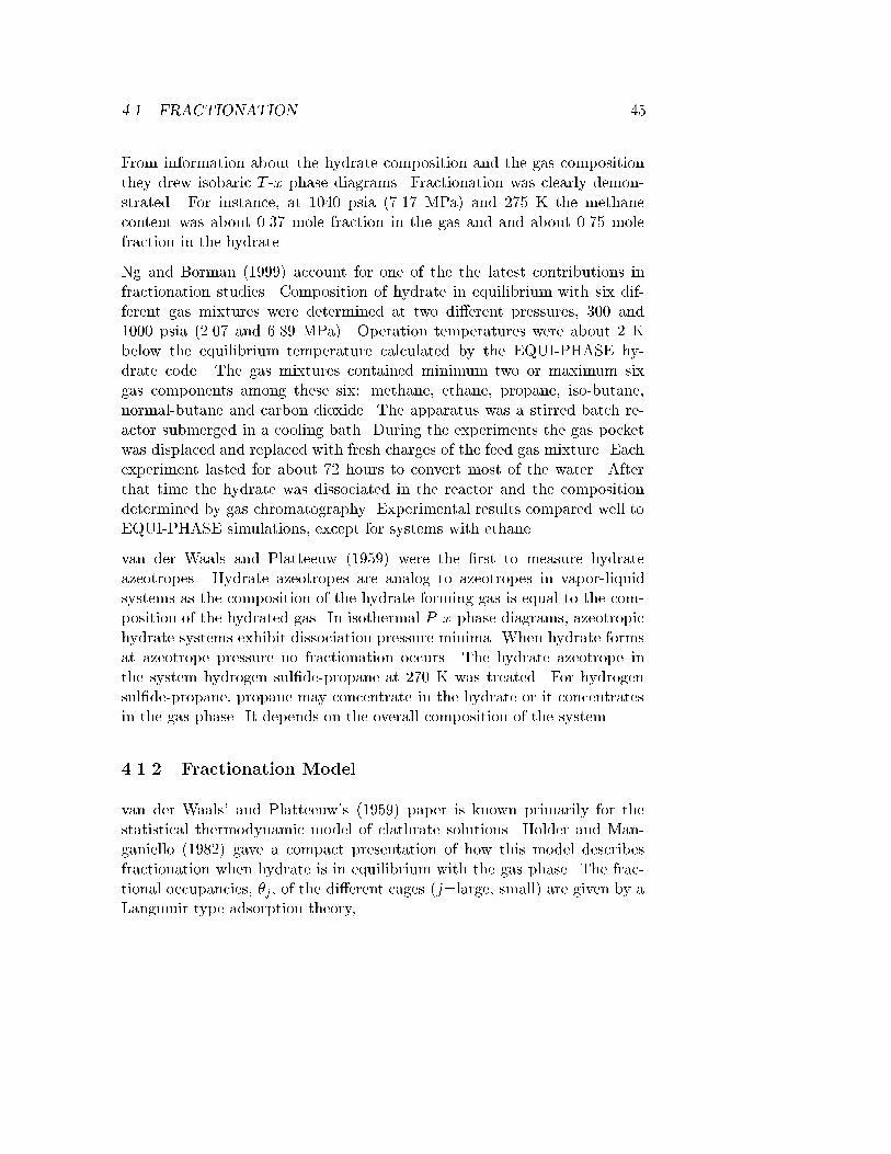
4.1. FRACTIONATION 45
From information about the hydrate composition and the gas compositionthey drew isobaric T -x phase diagrams. Fractionation was clearly demon-strated. For instance, at 1040 psia (7.17 MPa) and 275 K the methanecontent was about 0.37 mole fraction in the gas and and about 0.75 molefraction in the hydrate.
Ng and Borman (1999) account for one of the the latest contributions infractionation studies. Composition of hydrate in equilibrium with six dif-ferent gas mixtures were determined at two di�erent pressures, 300 and1000 psia (2.07 and 6.89 MPa). Operation temperatures were about 2 Kbelow the equilibrium temperature calculated by the EQUI-PHASE hy-drate code. The gas mixtures contained minimum two or maximum sixgas components among these six: methane, ethane, propane, iso-butane,normal-butane and carbon dioxide. The apparatus was a stirred batch re-actor submerged in a cooling bath. During the experiments the gas pocketwas displaced and replaced with fresh charges of the feed gas mixture. Eachexperiment lasted for about 72 hours to convert most of the water. Afterthat time the hydrate was dissociated in the reactor and the compositiondetermined by gas chromatography. Experimental results compared well toEQUI-PHASE simulations, except for systems with ethane.
van der Waals and Platteeuw (1959) were the �rst to measure hydrateazeotropes. Hydrate azeotropes are analog to azeotropes in vapor-liquidsystems as the composition of the hydrate forming gas is equal to the com-position of the hydrated gas. In isothermal P -x phase diagrams, azeotropichydrate systems exhibit dissociation pressure minima. When hydrate formsat azeotrope pressure no fractionation occurs. The hydrate azeotrope inthe system hydrogen sul�de-propane at 270 K was treated. For hydrogensul�de-propane, propane may concentrate in the hydrate or it concentratesin the gas phase. It depends on the overall composition of the system.
4.1.2 Fractionation Model
van der Waals' and Platteeuw's (1959) paper is known primarily for thestatistical thermodynamic model of clathrate solutions. Holder and Man-ganiello (1982) gave a compact presentation of how this model describesfractionation when hydrate is in equilibrium with the gas phase. The frac-tional occupancies, �j, of the di�erent cages (j=large, small) are given by aLangmuir type adsorption theory,

46 CHAPTER 4. FRACTIONATION - LITERATURE STUDY
�j =
PiCjifi
1 +P
i Cjifi(4.1)
where Cji is the Langmuir constant for gas component i in a type j cage andfi is the gas phase fugacity for gas component i. The Langmuir constantexpresses the a�nity a guest has to a cage. The fraction of j-type cagesoccupied by the i-type guest is:
�ji =Cjifi
1 +P
i Cjifi(4.2)
Makogon (1997) gives the fraction of all sII cages which are occupied byi-type guest as:
�i =16�s;i + 8�l;i
16P
i �s;i + 8P
i �l;i(4.3)
If the above equations are are combined with information about the hydratestructure (Section 2.1), then fractionation for a system in equilibrium canbe calculated.
fi is related to the mole fraction of i in the gas, yi, and to the pressure, P ,by
fi = �iyiP (4.4)
where �i is the fugacity coe�cient. Cji is a function of temperature onlyfor a gas component i with its properties �xed. The potential function w(r)describes the gas-water interaction and determines the Langmuir constant,
Cji =4�
kT
Z Rj�a
0exp
�wji(r)
kTr2dr (4.5)
where r is the radial position of an i-type gas molecule in a j-type cage whichhas a radius Rj. w(r) is expressed by the Kihara spherical core function,
w(r) = 2z�
"(��)12
R11r
��10 +
a
R�11��(��)6
R5r
��4 +
a
R�5�#
(4.6)

4.1. FRACTIONATION 47
where
�N =
h�1� r
R �aR
��N��1 + r
R �aR
�i�NN
(4.7)
and z is the number of water molecules that form the cage (the coordina-tion number). � (energy well depth), �� (modi�ed Kihara diameter) anda (core diameter) are the pair potential parameters for gas-water interac-tions. �� = � � a where � is the Kihara diameter, which is where the pairpotential is zero. A simple way to do manual calculations of the Langmuirconstants is to use the correlation Cji =
Aji
T expBji
T where Aji and Bji areempirical constants (Parrish and Prausnitz 1972). The original publicationsare referred to for detailed explanations.
Holder and Manganiello (1982) used van der Waals-Platteeuw theory toshow that hydrate azeotropes (no fractionation) may occur only in ternarymixtures (two guest gases and water), meaning that fractionation is boundto occur in systems with three or more guest gases. But among a selectionof gases; methane, ethane, ethene, propane, cyclopropane, iso-butane andhydrogen sul�de, hydrate azeotropes are predicted at 273 K for only a fewpairs; methane-propane, methane-cyclopropane, methane-isobutane, hydro-gen sul�de-propane, hydrogen sul�de-cyclopropane and hydrogen sul�de-isobutane. These are pairs of molecules where the smallest (methane or hy-drogen sul�de) �ts well into the smallest sII cavity and the largest molecule�ts well into the largest sII cavity. All these pairs form sII due to the sizeof the larger molecule.
Holder and Manganiello gave the following criterion for azeotrope formation:\In general, hydrates formed from a ternary mixture containing two hydrateforming gases and water will have a dissociation pressure for some mixturewhich is lower than any dissociation pressure of any binary mixture if andonly if one of the gases has a diameter ratio, �
d2, for the large cavity very
near 0.44 and the other gas has a diameter ratio, �d1, for the small cavity
near 0.44." � is the Kihara diameter and di is the cavity diameter for cavityof type i.

48 CHAPTER 4. FRACTIONATION - LITERATURE STUDY
4.1.3 Fractionation Simulations
The theory of van der Waals and Platteeuw has been implemented in com-mercially available computer simulation codes, for example CSMHYD fromColorado School of Mines (U.S.A.) and EQUI-PHASE from DB RobinsonResearch (Canada). These codes may be used to simulate fractionationwhen a hydrate is in equilibrium with the gas mixture. Required input isthe composition of the gas and either pressure or temperature.
Makogon (1997, pp. 43-47) used EQUI-PHASE to simulate fractionationof natural gas of methane (80 and 99 %vol) and ethane, propane, carbondioxide and butanes. He noted that the composition of the hydrate is de-termined mainly by the composition of the hydrate forming gas as well aspressure and temperature. Some conclusions were:
� The amount of a heavy component in the hydrate increases with themolecular weight.
� The amount of heavy components in hydrate decreases and methanecontent increases when both pressure and temperature increase.
� Hydrate formation pressure has the most signi�cant e�ect on thepropane and iso-butane content in hydrate.
� It is suitable to maintain low pressure and temperature during hydrate-based separation.
4.2 Driving Force
The studies in Section 4.1.1 reported hydrate compositions at or close tophase equilibrium. In the present work focus is on hydrate formation awayfrom the equilibrium curve. The purpose is to study hydrate compositionas function of the driving force. No papers which report a similar approachwere found. But work has been done on the e�ects of the driving force onkinetics, notably hydrate nucleation.
The driving force is generally an expression which represents the di�erencebetween the equilibrium value end the experimental value of some parame-ter. Sloan (1998, p. 98) listed di�erent driving force expressions that are inuse in nucleation modeling (Table 4.3).

4.3. DISCUSSION 49
Table 4.3: Driving forces in hydrate nucleation (Sloan 1998, p. 98).
Temperature Teq � TexpChemical potential �w(h);exp � �w(l);expFugacity
fi;expfi;eq
� 1
Free energy �Gexp
Teq � Texp is usually referred to as subcooling, as in this work, or as super-cooling. Relations between the driving force and the induction time are,without exceptions, stochastic and system dependent. The complexity ofhydrate kinetics accounts for the lack of deterministic models in the liter-ature. Instead, correlations and best �ts are determined. But the resultsfrom one laboratory can not be transferred to another laboratory or to the�eld to do reliable quantitative predictions (Sloan 1998, pp.98-103).
Sloan (1998) noted that there are few justi�cations based on equilibrium ornon-equilibrium thermodynamics for the driving forces listed above. Thusa general driving force derived from basic principles for T=constant is pro-posed:
�G = vw(Peq � Pexp) +RTX
xi lnfi;eqfi;exp
+ vh(Pexp � Peq) (4.8)
The �rst and last right hand terms are due to Pv di�erences between exper-imental (exp) and equilibrium (eq) conditions. Since the molar volume ofwater (vw) is within 15% of the molar volume of hydrate (vh), and since thesetwo terms typically are small compared to the RT � � � term, these Pv termse�ectively cancel.
4.3 Discussion
Fractionation Measurements
Both the apparatus of Happel et al. (1994) and that of Ng and Borman(1999) are well suited to study fractionation, but both could be improvedby implementing ideas from the other.
Happel et al.'s apparatus. From the gas entered the reactor at the bottomand till the unconverted portion of the gas reached the liquid surface, there

50 CHAPTER 4. FRACTIONATION - LITERATURE STUDY
must have been a shift in the gas composition in the bubbles. Consequently,the composition of the purge gas does not give the full picture - it is anapproximation. It may be better to feed the gas into the gas pocket andhave the gas sampling point far from the feed point, as in the apparatus ofNg and Borman. Happel et al. took small hydrate samples. Ng and Bormanallowed all of the hydrate to dissociate and then collected small gas samplesfrom the gas that evolved. It is easier to collect a representative gas samplethan a representative hydrate sample.
Ng and Borman's apparatus. To maintain a "constant" gas compositionthe gas pocket was from time to time displaced and replaced with freshgas. Between each displacement-replacement cycle, there must have been acontinuous shift in the gas pocket composition. It may be better to havean arrangement with continuous feed and purge, using the arrangement ofHappel et al.
Driving force
A suitable driving force is needed for the present work. If the driving forceis expressed as subcooling it becomes simple to quantify it. It is neces-sary to know the pressure and temperature and the hydrate equilibriumcurve. Both pressure and temperature are easy to measure directly. Theequilibrium curve is readily available with su�cient accuracy from computersimulations for the methane-ethane-propane-water system to be used in thepresent work. It is then easy to �nd the driving force, �T , simply by taking�T = Teq � Texp. If this formulation of the driving force is selected it isalso easy to log the driving force during the course of an experiment. Thisis an important consideration since it is necessary to maintain a drivingforce that is not only constant but has the desired value as de�ned in theexperiment plan. Another important consideration is that pressure can beregulated rapidly, while temperature regulation is usually much slower. Forthese reasons it was decided to express the driving force as subcooling, �T ,with unit K in the present work.
4.4 Important Findings
� van der Waals-Platteeuw theory can be used to calculate the compo-sition of hydrate in equilibrium with the hydrate forming gas. Thismakes it possible to calculate the fractionation in equilibrium systems.

4.4. IMPORTANT FINDINGS 51
� Fractionation will always occur for systems with three or more guestgases. Fractionation can only be avoided for a limited number of dou-ble hydrates (two guest gases).
� Experimental fractionation data in the literature are few, and only sys-tems allowed to form hydrate close to the hydrate equilibrium curvehave been studied. It seems the e�ect of the driving force on fraction-ation has not been reported earlier.
� The apparatuses of Happel et al. (1994) and of Ng and Borman (1999)are well suited to do fractionation studies.
� It is argued that subcooling is a suitable way to express the drivingforce in the present work.

52 CHAPTER 4. FRACTIONATION - LITERATURE STUDY

Chapter 5
Apparatuses
5.1 Introduction
Five laboratories were designed and built to study di�erent aspects of nat-ural gas hydrate. The laboratory with the most involved design was the ow loop laboratory for continuous hydrate production and sampling (Sec-tion 5.2). It had a 9 dm3 continuous stirred tank reactor (CSTR) and twoparallel ow lines where di�erent in-line test units (�lters, samplers etc.)were connected. The design pressure was 12 MPa and the ow line in-ner diameter was 20 mm. The volume of the loop was about 35-40 dm3,depending on the number and type of test units in use. Hydrate sam-ples removed from the ow loop were prepared in the cold laboratory (Sec-tion 5.3). In the climate laboratory (Section 5.5) for natural gas hydratestorage, temperature and air humidity could be controlled. After hydrateproduction, sample preparation and storage, samples could be analyzed inthe calorimeter laboratory (Section 5.4), featuring a low-temperature heat ow calorimeter, capable of operating at sample pressures of 10 MPa. Theselaboratories were built at NTNU in Trondheim. The batch reactor labora-tory (Section 5.6) to study fractionation in natural gas hydrate formationfeatured a 0.6 dm3 batch reactor and a gas chromatograph. It was built atthe National Polytechnical Institute in Toulouse in France. Other presen-tations of the laboratory facilities are those by Andersson (1999), Petersen(1997) and Gudmundsson et al. (1999).
53

54 CHAPTER 5. APPARATUSES
5.2 Flow Loop Laboratory
5.2.1 Conceptual Design
The purpose of the ow loop laboratory was hydrate production and sam-pling. To justify the conceptual design it is useful to review the objectivesof the laboratory and some basic requirements. The main objectives were toproduce hydrate for subsequent analysis of thermophysical properties, andto collect operational experience and data on hydrate slurries and contin-uous hydrate production. This would provide essential engineering inputwhen upscaling to a pilot plant, as well as constituting fundamental science.
The ow loop was not supposed to imitate the future large scale process.However, the hydrate production conditions had to have relevance to theexpected future, and a reasonable pressure for the future large-scale processwas assumed to be 6 MPa. A design pressure of 12 MPa, the double of6 MPa, was de�ned.
The large-scale process for natural gas hydrate production was, and is stilltoday, likely to be a train with one or more reactors of some kind. The closestthing within the economical constraints was a ow loop with a hydratereactor. A CSTR with standard design was chosen since performance andupscaling correlations of such reactors are known. A circulation pump wasneeded to circulate the condensed phase. Heat of hydrate formation hadto be removed in a heat exchanger. A separator was necessary to handleunconverted gas. Filters were the �rst choice for hydrate sampling.
It was desirable to operate the reactor (well) within the hydrate pressure-temperature region while at the same time having the option to operatethe rest of the loop nearer the hydrate equilibrium curve at a lower pres-sure. To boost the pressure at the reactor inlet, the pump had to be thelast unit preceding the reactor and a pressure reduction valve the �rst unitdownstream of the reactor. It was desirable to remove gas bubbles beforethe slurry entered the test sections. Thus the separator would follow down-stream of the pressure reduction valve, and then the two parallel test unitlines downstream of the separator. The test sections needed a bypass line.The heat exchanger had the greatest potential for plugging, both becauseof its internal geometry and since this was where the temperature would belowest. Being conservative, the heat exchanger was placed after the �lter(test section). The heat exchanger was the last unit before the pump. Thus,

5.2. FLOW LOOP LABORATORY 55
the pressure would be relatively low in the heat exchanger, making hydrateformation in the heat exchanger less likely. Having decided about the mainunits and their order, the basic ow sheet in Figure 5.1 was settled.
Choosing standard type of equipment whenever possible and suitable wassettled as a basic rule in the concept phase and remained an important guide-line. Standard equipment is less expensive and has a shorter delivery time.Another guideline was to have exibility in mind during design and modi�-cations. The purpose was to be able to operate the loop in di�erent modesand preparing for tasks that were not foreseen at the time. Realizations ofthis design philosophy was for example the bypass lines and the numerousblinded tees where tubing or sensors could be connected as needed. Anotherexample is that the reactor and the separator had identical measures exceptthe separator was twice the length of the reactor. Parts that �tted one �ttedthe other as well. Yet another example is the gas supply system with twoparallel gas supply lines. It was possible to change from one gas tank to another in practically no time. This guaranteed continuous gas supply. It alsogave the option of changing from one feed composition to another simply byswitching valves.
The ow loop was going to be used with water and petroleum uids. Saltsand low-dosage hydrate promoters would be added in some experiments.Thus it was decided to go for stainless steel in all units as well as in tub-ing and �ttings. For safety reasons it was decided that all electrotech-nical and electronic installations in the room should be classi�ed for in-stallation in hazardous areas. All units were mounted on a wheeled skid(HxWxL=2.0x1.0x2.2 m3).
5.2.2 Room Temperature
To have better control of the temperature, the ow loop was placed in aroom where the temperature could be regulated between 273 and 298 K. Anoven on the wall provided excessive heating, if needed, and the temperaturewas regulated by a thermostated air conditioner. The idea was to keep theroom temperature at the operation temperature. This gave good control ofthe temperature in all places in the loop. It was a way of minimizing thetemperature gradients in the loop. There were no temperature irregularitieswhich caused hydrate dissociation (hot spots) or hydrate deposition (coldspots).

56 CHAPTER 5. APPARATUSES
Cooling
Gas feed
REACTOR SEPARATOR
TESTSECTION
orFILTER
HEAT EXCHANGERCIRCULATION PUMP
Pressurereductionvalve
Gas purge
Water feed
Figure 5.1: Conceptual loop design showing the main units. The second testsection line and the test section bypass line are not shown.
After collecting hydrate in a �lter, the �lter was isolated. If the room tem-perature had not been close to the operation temperature, hydrate wouldsoon start to dissociate. But since the room temperature was low and thepressure equal to the operation pressure, the hydrate in the isolated �lterwas thermodynamically stable. There was still no risk of hydrate dissoci-ation when displacing the �ltrate (details later). It was also an importantrequirement in the studies of hydrate slurry rheology, that the temperatureof the slurry was well de�ned and stable (Andersson 1999).
5.2.3 Main Units
Reactor
A CSTR reactor with a standard design was chosen, since the performanceand up-scaling of such reactors are well described in the literature. Thereshould be nothing special about the reactor, just ba�es, an impeller, inletsand outlets. The only extra thing was the two sparged gas inlets and theview-ports for visual observation and video monitoring. The reactor volume

5.2. FLOW LOOP LABORATORY 57
was settled at 9 dm3. This volume was 15 times larger than the batch reactor(0.6 dm3) that had been used previously, and about an order of magnitudesmaller than what was regarded as a reasonable reactor volume in a futurepilot plant.
The reactor inner length/diameter ratio was LD = 378=180 mm/mm. The
ba�es extended about D=10 from the wall. The impeller diameter wasabout D=2:5 and it was placed D=2 above the bottom. The lower inlet andoutlet ports were also located D=2 above the bottom. The upper ports werelocated the same distance below the top. The reactor ports could be usedfor ow inlet or outlet, or they could be used as view-ports or be blinded.There was also the possibility of using the ports for sensors of di�erentkinds. A total of eight ports were symmetrically placed on two levels. Thedesign details were proposed by Proserv who also fabricated the reactor andseparator.
The impeller was a straight blade turbine with six blades. It generates radial ow and is especially suited for dispersion of gases in liquids. It was drivenby an Autoclave Engineers Magnedrive and could be operated at any speedbetween 0 and 2500 RPM. The rotation speed was measured and showed ona display.
The gas spargers dispersed the gas, making mass transfer more e�cientcompared to non-sparged inlets. The two spargers were placed oppositeeach other, at the same distance from the center of the reactor bottom.This distance was equal to the radius of the impeller. Thus gas was injectedat a point close to and just below where the stirring was most vigorous,at the tips of the impeller. The spargers were specially made from smallstainless steel cup �lters (7 �m) with outer diameter of about 1 cm and alength of about 2 cm. The spargers also held small check-valves to preventwater back ush into the gas feed line.
The reactor liquid (slurry) feed came from the heat exchanger and it wasdesirable to instantly distribute the feed throughout the reactor. Thus thewater or slurry was fed to the reactor through one of the lower ports in thelevel of the impeller. The outlet line was connected to one of the upperports.
The unit downstream of the reactor was a Tescom pressure reduction valve.It was only used during some early tests and then dismounted. The perfor-mance of the valve was not as desired. The valve had no signi�cance to thework presented here and is not mentioned further.

58 CHAPTER 5. APPARATUSES
Separator
The main purpose of the separator was to separate unconverted gas forpurging. Its length was twice the length of the reactor. Other dimensionswere the same, giving a separator volume of 18 dm3. It had four upper(lower) ports placed at the same distance from the top (bottom) as in thereactor. Because of the separator length it was given four additional portsin two intermediate levels. The separator volume was about half of the totalloop volume.
To avoid gravity separation of hydrate and water in the separator, mixingwas provided by a mixing pump. It was a Haskel piston pump which circu-lated slurry from the bottom of the separator to the top via an external line.Should it be desirable to concentrate the hydrate in the separator separate,the mixing pump was simply not used. Hydrate was then retained in theseparator which served as a hydrate holding tank. An exit line for hydratelean slurry was connected to a lower port. An exit line for hydrate richslurry was connected to an upper port. The ow sheet in Figure 5.2 onlyshows the upper exit line.
Test Units
Several types of test units were available. Only cup �lters were used in thiswork. The �lter units consisted of the actual �lter cup, a perforated supportbasket for the �lter cup and a pressure cell with inlet and outlet valves. Twotypes of �lter cups were used; K�opp porous polymer cups and in-house madecups made from stainless steel mesh. K�opp �lter grades of 5, 25 and 80 �mwere used. Mesh �lter grades were 77 and 510 �m. The inner length anddiameter of the polymer cups were 16 and 6 cm, respectively. This yieldeda cup volume of about 0.45 dm3. The mesh �lters were somewhat larger.Apart from the �lters, a Fras Technology sampler, an in-house tube sampler,a thin-section glass cell and a specially designed tube viscometer were alsoavailable and used by Andersson (1999).
The purpose of the support basket was to hold the �lter cup in the desiredposition and to prevent rupture of the �lter cloth due to the pressure dropacross it. The basket was made from perforated steel plates. The innerdimensions of the support basket �tted closely to the outer dimensions ofthe �lter cup. The basket top ange served as a positioner for the basketand thus for the �lter. To direct the slurry through the �lter, the ange wasdesigned as a double ange with O-rings at critical places.

5.2. FLOW LOOP LABORATORY 59
Test unit bypass
PT
P
T
P TdP
PdP
TP
P
P
P
PP
PT
T
T
T
T
Separator
21
Gas
Gas
Flow
met
er
Cir
cula
tion
pum
p
VFM
gB
PR
Hea
t Exc
hang
er
Vie
w
serv
ice
boos
ter
VFM
g
bottl
es
Gas
Tes
tT
est
unit
unit
Sepa
rato
r by
pass
Sepa
rato
r by
pass
Reactor
Figure 5.2: Detailed ow sheet of the ow loop laboratory. P and T arepressure transducers and thermocouples, respectively. dP connected to thedi�erential pressure cell. VFMg are gas ow meters. BPR is the backpres-sure regulator.

60 CHAPTER 5. APPARATUSES
The pressure cell was necessary to enable inline �ltration at elevated pres-sures. The only dimensional requirements were that a �lter cup of aboutone liter should �t into it and it had to withstand the design pressure.
During �ltration it was possible to measure the pressure drop across the �l-ter by a di�erential pressure gauge. After �ltration, the annulus between thesupport basket and the walls of the pressure cell was full of �ltrate (water).It was necessary to displace this liquid while maintaining the desired pressureinside the pressure cell. A special valve arrangement was made for the pur-pose, as illustrated in Figure 5.3. With this arrangement a high-pressure gasof choice could be fed to the pressure cell. The gas ow rate was controlledby the needle valve. As gas was fed through the top, water was displacedthrough the bottom. The pressure inside the pressure cell was maintainedby a relief valve. Upon gas break-trough all of the water had been displaced.The valve arrangement together with the valves permanently mounted onthe pressure cell caps constituted a double block and bleed system. This wasnecessary since the quick connects could not be opened when pressurized.The ow loop also had double block and bleed valves so that test sectionscould be connected and disconnected while operating the loop.
relief valveNeedlevalve
Quickconnect
Quick
Gassupply
Double block bleeders
Filter
TOPAdjustable
bleederFiltrate
connect
BOTTOM
Figure 5.3: Valve arrangement used to displace the �ltrate from the �l-ters while maintaining the hydrate production pressure. The double blockand bleed arrangement was necessary since the quick connects could not beopened while pressurized.
Heat Exchanger
The purpose of the heat exchanger was to maintain constant temperaturein the high-pressure loop. The heat exchanger was a shell-and-tube type,made by Sperre Industri. The main reason for this choice was that the hot

5.2. FLOW LOOP LABORATORY 61
side should have a high design pressure, 12 MPa. For exibility reasons theheat exchanger was made so that the cold side also could withstand thispressure. The hydrate slurry was on the tube side and the glycol/watercooling media on the shell side. The reason for this con�guration was thatif hydrate plugging occurred, it would be easier to remove small cylindricalplugs inside the tubes than a larger irregular plug extending throughoutmost of the shell side and immobilized by the tubes penetrating it.
The cold and hot streams in the shell-and-tube exchanger followed a cross-counter ow pattern. Circulation of cooling media was maintained by a cen-trifugal pump that worked at constant speed. The duty of the heat ex-changer was regulated by a three-way Samson regulating valve. The coolingmedia ow was constant and the valve directed a proportion of this owthrough the heat exchanger. The regulator received temperature signalsfrom one of two optional temperature sensors, one in the reactor and onein the hydrate slurry line line just down-stream of the heat exchanger. Tomaintain a low temperature in the cooling media, the cooling circuit featureda plate heat exchanger where the cooling media could give away heat to asecondary cooling media (propane). The secondary cooling media exchangedheat with the surroundings in a cooling machine placed out-doors.
If particles or fouling in the cooling circuit should come loose and becometrapped in the regulating valve it could malfunction. As a precaution a �lterwas placed close to the inlet of the regulating valve. For the same reason, andalso to prevent poorer heat transfer with time, the cooling media containeda biocide to prevent algae growth. For the regulating valve to functionproperly there had to be a certain pressure drop in the cooling circuit. Bypartially closing a ball valve in the cooling circuit extra pressure drop couldbe generated, if needed. The cooling circuit also had an air trap with a bleedvalve at the highest point and a drain valve at the lowest point. A turbinemeter in the cooling circuit and temperature sensors to measure the coolingmedia's temperature increase provided data to accurately calculate the heatexchanger duty.
Circulation Pump
Originally a piston pump identical to the separator mixing pump was usedas a circulation pump. It was decided to try this pump type since it was alot less expensive than the alternatives. After some time of testing it wasclear that the pressure pulses that the pump generated made it unsuitable.

62 CHAPTER 5. APPARATUSES
The primary reason was that the tube viscometer required non- uctuating ow.
The pump types that were considered then were monopumps and centrifu-gal pumps. Both are suitable for slurry pumping and were considered goodalternatives. In a monopump particles of considerable size may get throughthe pump without being crushed. In a centrifugal pump the particles aremore likely to be crushed from mechanical impact. Still, a Caster centrifugalpump was chosen for economical reasons. The ow could be regulated be-tween zero and about 100 dm3/min, depending on the pressure drop throughthe loop. The pressure drop depended on which units were bypassed andwhich were not, and the viscosity of the uid.
5.2.4 Utility Units
Compressor
Gas could be fed to the reactor directly from the gas tanks. But if thetank pressure was below the operation pressure the gas needed boosting. AHaskel piston compressor was used. Pilot valves on the compressor startedand stopped the compressor automatically whenever needed.
Water Feed Pump
There were two ways to feed liquid to the loop. Before pressurization, waterwas usually sucked into the loop after evacuating it. This gave full controlof the water volume and air pockets were completely avoided. If it wasnecessary to inject water while the loop was pressurized, this was done bythe water feed pump; a Haskel piston pump. The stroke volume of the pumpwas small (2.14 cm3) and one by one stroke could be made through manualoperation. This made it suitable as a dosage pump for additives. By addingdiluted additives and by performing the injection over a time that was atleast as long as the loop circulation time, the additives could be fairly welldistributed throughout the slurry volume. The injection point was at thepump inlet to bene�t further from the mixing in the volute.

5.2. FLOW LOOP LABORATORY 63
Degasser
To avoid e�ects from air dissolved in the water, the water was degassedbefore it was transfered to to the loop. Degassing took place in a speciallydesigned vacuum tank. A �lter between the tank and the loop removedparticles in the feed water. The main reason for �ltering the water was thatparticles such as sand could damage the valves in the loop. The degasserand its connections are shown in Figure 5.4. The tank was mounted on arocking skid so that it could be rotated manually almost 360�. Thus thetank was also suitable for preparation of solutions or emulsions in volumeslarger than the loop volume. After degassing the tank could be moderatelypressurized with a gas, typically methane, and water sucked/displaced intothe loop. Alternatively, water could be directed to the water feed pump forhigh-pressure injection.
pump
Vacuumpump
NGH flow loop
BleedTap water
Filter
Vent
Safetyvalve
P
Cap
V=80 literT
Degasser
Gas
Waterfeed
Figure 5.4: The degasser.

64 CHAPTER 5. APPARATUSES
Vacuum Pump
The vacuum pump had two uses. It could be used to evacuate the degasser.Consequently the water would give o� its dissolved air. Better control withthe overall composition of the system in the loop was obtained. After de-gassing, the degasser could be moderately pressurized with a gas, usuallymethane.
The other use of the vacuum pump was to evacuate the ow loop. Thenthe loop could be connected to the degasser and a desired amount of waterwould ow quickly into the loop. The vacuum pump was made by Leyboldand had a �nal pressure of < 10�2 Pa.
View-port
The value of visual observations was expected to be high. Qualitative infor-mation could help understanding the system. Thus a view port was placedin the ow loop, downstream of the test sections. It would then be possibleto observe the e�ect of �ltration. By bypassing the �lters it would also bepossible to determine how long it would take to make hydrate particles largeenough to be observed visually. This could be a quantitative, although notdeterministic, way to describe di�erent systems. Studies of agglomerationand particle size were also among the foreseen uses of the view-port. It hada light opening of 38 mm and with two windows placed on opposite sidesof the ow. Thus it was possible to look "through" the slurry and not only"on" the slurry.
Valves, Fittings and Tubing
The main criteria when selecting valves and �ttings were that all items hadto be made of stainless steel and all items had to be available within thesame �tting system. Swagelok �ttings and Whitey valves were chosen. Themain loop with bypass-lines had 25 mm tubing with 20 mm inner diameter.Gas lines were made from 6 mm tubing. Flexible hoses with quick connectswere used between the test units and the rest of the loop. Double blockand bleed arrangements were necessary since the quick connects could notbe opened while pressurized. Numerous special parts were made at thein-house mechanical workshop.

5.2. FLOW LOOP LABORATORY 65
5.2.5 Instrumentation, Regulation and Logging
Pressure
Pressure was measured by Keller pressure transducers. They were placedupstream and downstream of all main units. For the reactor and separa-tor, the pressure was measured in the units as well. See Figure 5.2. Thetransducer range was 0 to 10 MPa. Pressures at each measuring point wereshown on displays placed on one of the walls in the ow loop laboratory.The pressure pro�le in the loop could then be monitored in real-time.
There were two ways to regulate the pressure, depending on the mode ofoperation. Usually, there was a continuous supply of gas that exceededthe gas conversion rate. The excess gas collected in the separator and waspurged through a back-pressure regulator to the vent line. Thus constantpressure was maintained. Alternatively, the purge line was closed. Pressurewas then regulated by setting the gas supply pressure somewhat higher thanthe operation pressure and supply gas through a needle valve, as seen onthe ow sheet. The pressure drop over the needle valve and the spargersaccounted for most of the pressure di�erence between supply pressure andoperation pressure.
Temperature
PT-100 temperature sensors were placed together with the pressure trans-ducers, upstream and downstream of all main units, as well as in the reactorand the separator. There was a display for each temperature sensor so thetemperature pro�le in the loop could be read at any time.
The temperature was regulated by the regulating valve in the cooling cir-cuit, as described earlier. To have even better control with the temperature,the whole ow loop was placed in a thermostated room. Room temperaturecould then be set at the operating temperature. This gave a atter temper-ature pro�le. There was also a sensor to measure the room temperature.
Di�erential Pressure
The pressure drop over a test section was measured by a Fuji Electric dif-ferential pressure sensor. The main purpose was to monitor the pressure

66 CHAPTER 5. APPARATUSES
drop during �ltration. This gave information about how the �ltration wasprogressing, as a thick �lter cake gives a high pressure drop.
Gas Flow
Bronkhorst gas ow meters were installed on the gas supply line and on thegas vent line. The gas ows were shown on displays on the wall in the owloop laboratory. The gas ow meters with the displays were necessary to beable to regulate the gas supply rate. Regulation was done manually. Theparameters that together determined the gas supply rate was the opening ofthe needle valve on the gas supply line and also the di�erence between the gassupply pressure and operation pressure. Gas ow data were also necessaryto establish the mass balance, since the di�erence between supplied gas andpurged gas was accounted for by the hydrated gas, the gas pocket in theseparator (and gas bubbles) and dissolved gas.
Liquid Flow
The liquid or slurry ow in the ow loop was measured by a Fisher-Rosemontcoriolis meter. The ow rate was controlled by manually regulating the speedof the circulation pump.
In the cooling circuit there was a Nixon Instrumentation turbine meter whichmeasured the cooling media ow rate through the heat exchanger. Thismeter too had a wall-mounted display connected to it. The circulationpump in the cooling circuit worked at constant speed. The ow rate ofcooling media through the heat exchanger was regulated automatically bythe regulating valve, as described above.
Data Logging
A large number of electronic measuring devices have now been described.Every one of them gave a continuous analog signal that was collected bythe data logger installed on a personal computer. LabVIEW was used tocollect the data. The user interface displayed the pressure and temperaturesat di�erent positions in the ow loop. The pressure drop over the �lter (testsection) was also displayed, as was the gas ow rate in the supply line andthe purge line. Data from every sensor were available, in real-time and in

5.2. FLOW LOOP LABORATORY 67
the log �les. The logging frequency was set by the operator and could bechanged at any time during an experiment.
5.2.6 Safety
Important safety issues were preventing gas leakages, preventing ignitionshould there still be a leakage, and preventing the loop pressure to exceedthe design pressure. Line rupture valves were mounted on the two parallelgas feed lines as well as at the compressor outlet. If an explosive atmo-sphere were created after all, the probability of ignition was small since allelectrical and electronic installations, sensors and transmitters as well asswitches, lightening and air conditioning, were intrinsically safe and clas-si�ed for installation in hazardous area zone 2 where, by de�nition, \anexplosive gas/air mixture is not likely to occur in normal operation, and ifit occurs it will exist only for a short time".
A combustible gas sensor was used routinely to monitor the contents ofhydrocarbons in the air. Two ventilation fans were installed, one whichdrew air from the laboratory and an other which supplied fresh air. A 2 m2
relief panel was placed on one of the walls.
If there was a malfunction of the gas supply system or the operator made anerror, it could be that the pressure would exceed the design pressure. Safetyvalves relieved excess gas through a vent line. To qualify the ow loopfor operation at pressures up to the design pressure it was pressure testedat 15 MPa, a pressure which exceeded the design pressure by 25%. Thepressure test was carried out by using the water feed pump to completely�ll and pressurize the loop with water. The test pressure was maintainedfor 30 minutes.
5.2.7 Miscellaneous
Video equipment
A Sony video camera was used to record the slurry passing through theview-port downstream of the �lters. A Sony micro camera was small enough(12 mm diameter) to �t into the windows of the reactor and separator, andwas used together with the thin-section glass cell too. It had a speciallymade system for back-lightening. Video images could be exported to the

68 CHAPTER 5. APPARATUSES
Optimas image processing software. These facilities were primarily usedby Andersson (1999) in the studies of hydrate slurry rheology.
Control Room
The situation in the ow loop laboratory could be monitored from the con-trol room in a neighbouring building. It was necessary to have such a room,since the laboratory was noisy, cold and drafty. In the control room, alllogging channels could be read at any time. A video monitor gave quali-tative information regarding slurry appearance and hydrate content. If thecirculation should stop, this would bee seen immediately.
5.3 Cold Laboratory
The purpose of the cold laboratory was to prepare hydrate samples. Theroom had temperature regulation down to nearly 250 K and was placednext-door to the ow loop laboratory. The cold laboratory was necessary tofreeze the �lter cakes, for sample preparation and for placing samples in thecalorimeter sample cell. All this had to take place at temperatures equal toor below the hydrate storage temperature, i.e. well below 273 K. The roomcontained a sturdy working bench with a vise and a saw that were used tocleave the �lter cups with the frozen �lter cake. A porcelain mortar and arange of sieves (1-10 mm, �0.2 mm) were available for samples preparation.
A portable glove compartment was available when transferring the calorime-ter sample cell from the cold laboratory to the calorimeter laboratory in aneighbouring building. The glove compartment was �lled with nitrogen.The idea was to prevent frost deposit on the sample cell as this would bea source of error in the measurements. A balance (�0.01 g) was used tomeasure the sample mass.
5.4 Calorimeter Laboratory
The purpose of the calorimeter laboratory was to measure thermophysicaland compositional properties of hydrate in the hydrate-ice samples that wereobtained from the ow loop laboratory. The calorimeter laboratory featuredthe main analytical instrument used in this work, a Setaram BT2.15 heat

5.4. CALORIMETER LABORATORY 69
ow calorimeter. Important requirements when choosing a calorimeter werethe possibilities to operate at temperatures well below 273 K and pressur-ize the sample with a gas of choice. The sample cell volume should beseveral cm3, since large samples were desired to suppress e�ects of sampleinhomogenities. Also, a similar calorimeter had been used by (Handa 1986a;Handa 1986b; Handa 1986c) to do experiments that had similarities to whatwas planned in this work. The calorimeter laboratory was placed in the sameroom as the climate laboratory.
Figure 5.5 shows the calorimeter and attached units. It contained two iden-tical cells; the sample cell (S) and the reference cell (R). A temperaturesensor for measuring the sample temperature was placed near, yet outside,the sample cell. Both cells were placed in a thermal block with heat uxmeters surrounding the cells. Electrical heating was supplied if requiredaccording to the temperature program (see below). Excessive cooling wascontinuously provided by saturated nitrogen (77 K). The nitrogen gas wascontinuously supplied from a liquid nitrogen tank that had a heating elementfor nitrogen vaporization. Nitrogen that had gone through the calorimeterand absorbed heat was vented to the surroundings.
The tubing arrangement included a pressure transducer, a pressurized gastank and valves. It was possible to adjust the pressure accurately in the twocells. The arrangement also made it possible to remove undesired gas(es)from the cells, either by evacuation or by pressurization-depressurizationcycles. The cell pressure was logged with LabVIEW.
Two modes of operation were possible; scanning mode and isothermal mode.A period with either scanning operation at a constant temperature transientor isothermal operation at a constant temperature is called a sequence. Atemperature program is made from one or more sequences. The calorimeterwas controlled by the SetSoft computer program which accompanied thecalorimeter. The temperature programs were edited in SetSoft which alsohandled the logging of sample temperature and heat ow as function of time.
Two types of calorimeter cells were used in this work. The one used toanalyze hydrate was an open cell with a volume of 8.5 cm3 and with a tuberod, hence it was possible to control the pressure inside the cells between0 and 10 MPa. The other type of cell was a closed cell with a volume of12.5 cm3 and with a solid rod. It was used in some introductory experiments.A Mettler balance (�0.002 g) was also available.

70 CHAPTER 5. APPARATUSES
Logging
P
S R
Bleed
Methane
Needlevalve
Bleed
Calorimeter
Figure 5.5: The calorimeter with attached units.
5.5 Climate Laboratory
The purpose of the climate laboratory was to store hydrate samples undercontrolled climatic conditions, including temperature and composition of theatmosphere, notably relative humidity. The climate laboratory was designedfor metastable storage of refrigerated hydrate at ambient pressure (1 atm).
It was decided to go for a solution with desiccators and Sanyo laboratoryfreezers. Hydrate was put in a desiccator and the desiccator in a freezer. Therelative air humidity in the desiccator was maintained at about 100 %RH byplacing crushed ice in the bottom. Dry air was obtained by using silica gel.It was also possible to add gases, such as methane, to alter the compositionof the atmosphere surrounding the hydrate sample. Temperature could becontrolled in intervals of 1 K between 224 K and 278 K (�2 K).
A Vaisala sensor for temperature and relative humidity was placed in oneof the desiccators. A pressure transducer was also placed inside the desic-cator. The sensors gave continuous logging signals. These were collected byLabVIEW installed on a personal computer. In other desiccators relativehumidity and temperature were measured by traditional analog instrumentsthat were read manually. The accuracy of these varied. The relative humid-ity meter had a larger error for temperatures below 273 K.
One of the freezer cabinets could be used to do storage experiments at di�er-

5.6. BATCH REACTOR LABORATORY 71
ent temperatures. In the other cabinet �lter cakes were kept at the lowestpossible temperature, 224 K. Samples could later be prepared from thesecakes. One household freezer was available for storage at about 255 K. Onehousehold freezer was modi�ed, and had temperature regulation betweenbetween 255 K and 273 K.
5.6 Batch Reactor Laboratory
5.6.1 Concept
The purpose of the batch reactor laboratory was to study fractionation whena gas mixture forms hydrate. There were two basic requirements; controlledand repeatable conditions during hydrate production and ability to performquantitative analysis of gas mixtures. A batch reactor with pressure regu-lation immersed in a water bath with temperature regulation was the usedto produce hydrate (Figure 5.6).
A gas chromatograph with a ame ionization detector was used for gas anal-ysis. The gas chromatograph sampling line could be connected to di�erentgas sample sources, notably a dissociation cell, the reactor or the bottle withcalibration gas. A household freezer (252 K) was used to stabilize the hy-drate by refrigerating it while it was still in the reactor and at the hydrateproduction pressure.
5.6.2 Reactor
The assembly for hydrate production is shown in Figure 5.6. The reactorwas a stirred batch reactor made of stainless steel. This was the same reactorused by Gudmundsson et al. (1994). Inner diameter was 75 mm and innerlength was 140 mm, yielding a volume of about 600 cm3. The stirrer wasa shafted, plastic coated, magnetic bar. Two small bolts on the reactorbottom ba�ed the water, although their primary function was to �x a rodwhich served as an upper shaft bearing. The magnetic bar was rotated by amagnetic stirrer placed under the reactor. The reactor had two ports withclosing valves on the wall. One port was connected to an Alcatel vacuumpump which gave a �nal pressure of 5 Pa. The other port was connected toa gas supply line. The top cap of the reactor could be removed to get accessto the hydrate. The bottom cap with the stirrer could also be dismounted,

72 CHAPTER 5. APPARATUSES
Vacuumpump
Excessivecooling
Tempreg.
PC, datalogger
Magneticstirrer
Insulatedwater bath
Temperaturesignal
Pressure Pressuresignal regulation signal
Pressuretransducer
Regulatingv alv e
Samplingv alv e
NG
bottle
Reac-tor
PID
Stirrer
Figure 5.6: Laboratory for hydrate production to study fractionation.
although this was never done during everyday operation.
The reactor was placed in a water bath with good mixing. A cold sinkwhich provided excess cooling exchanged heat with the water bath. Bathtemperature was kept constant by a thermostatic heater, thus the reactortemperature was regulated indirectly. It was taken into account that dur-ing hydrate production the reactor temperature was typically 0.3 to 0.5 Kabove the cooling water temperature. The reactor temperature was readby a PT-100 sensor in a thermopocket and the cooling water temperatureby a thermocouple. The pressure in the reactor was read by a pressuretransducer. Via a PID regulator, the transducer gave a signal to a pressureregulating valve. The reactor was operated within �0.5 K of the temper-ature set point and within �0.2 MPa of the pressure set point. Reactorpressure and temperature as well as cooling bath temperature were loggedby a personal computer using the Synchronie logging program.

5.6. BATCH REACTOR LABORATORY 73
5.6.3 Gas Analysis
The gas samples that were injected to the gas chromatograph were of threedi�erent categories; calibration gas, gas from the gas cap in the reactor atthe end of the hydrate production period and gas from dissociated hydrate.Calibration gas was injected from the gas bottle. Reactor gas was injecteddirectly from the reactor. Gas from dissociated hydrate was injected froma dissociation cell with a volume of about 80 cm3. The cell was made fromtubular heavy-duty transparent plastic with threaded ends for the caps. Itwas possible to visually observe the hydrate sample as dissociation pro-ceeded.
An Intersmat IGC 120 DFL gas chromatograph with a loop (0.3 cm3), aporapak N 80-100 column (�2 m) and a ame ionization detector was usedto make quantitative analysis of methane, ethane and propane. The tem-perature program had three sequences; an isotherm (351 K, 1.5 min), aramp (20 K/min) and a �nal isotherm (403 K) which lasted long enough forpropane to elute. The gas in the loop was injected after a static period (6 s)to make the total molar amount of gas in the loop approximately equal in allinjections. A Hewlett-Packard HP 3396 series II integrator was used to per-form peak integration. Normalized concentrations were calculated from themeasured chromatographic areas. Absolute concentrations were not needed.

74 CHAPTER 5. APPARATUSES
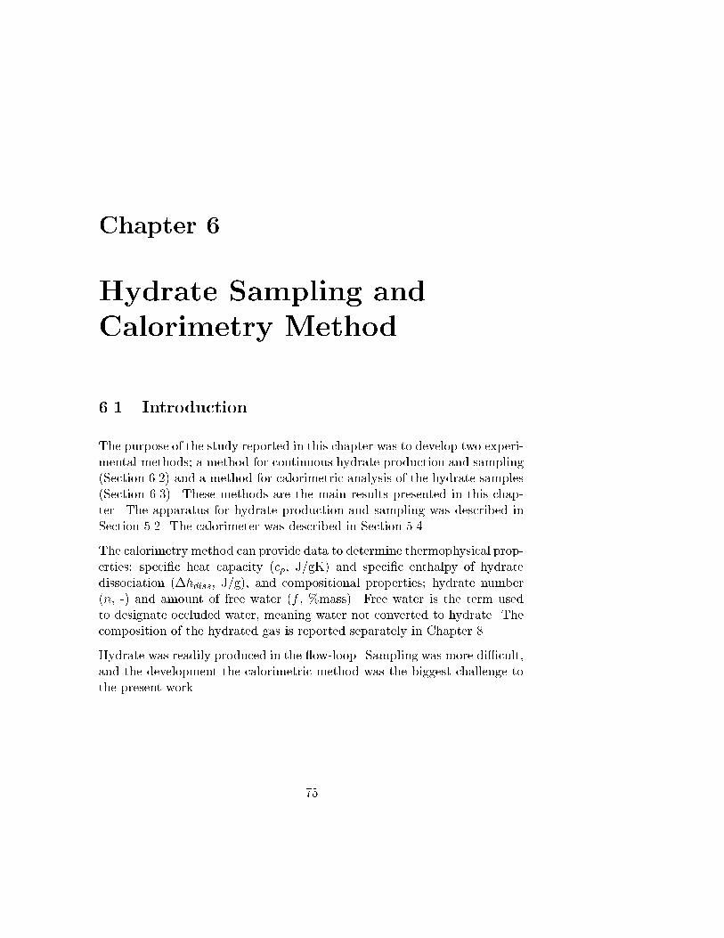
Chapter 6
Hydrate Sampling and
Calorimetry Method
6.1 Introduction
The purpose of the study reported in this chapter was to develop two experi-mental methods; a method for continuous hydrate production and sampling(Section 6.2) and a method for calorimetric analysis of the hydrate samples(Section 6.3). These methods are the main results presented in this chap-ter. The apparatus for hydrate production and sampling was described inSection 5.2. The calorimeter was described in Section 5.4.
The calorimetry method can provide data to determine thermophysical prop-erties; speci�c heat capacity (cp, J/gK) and speci�c enthalpy of hydratedissociation (�hdiss, J/g), and compositional properties; hydrate number(n, -) and amount of free water (f , %mass). Free water is the term usedto designate occluded water, meaning water not converted to hydrate. Thecomposition of the hydrated gas is reported separately in Chapter 8.
Hydrate was readily produced in the ow-loop. Sampling was more di�cult,and the development the calorimetric method was the biggest challenge tothe present work.
75

76 CHAPTER 6. PROPERTIES - RESULTS
6.2 Method for Continuous Hydrate Production
and Sampling
The ow loop where hydrate was made is described in Section 5.2. Andersson(1999, pp. 53-56) gave a description of hydrate production which stressesthe slurry related issues. The hydrate used in the present work was madefrom degassed tap-water and a gas mixture containing ethane (5 %mol) andpropane (3 %mol) in methane. The water was prepared in the degasser,described in Section 5.2.4. Tap water was degassed by vacuum boiling atabout 0.2-1 kPa. After degassing the degasser was pressurized to about0.3 MPa using methane. The ow-loop was evacuated. The degasser andthe loop were connected and water was displaced into the loop. In thismanner the loop was �lled with any desired amount of water, leaving agas cap in the separator. Next, the loop was pressurized to just below thehydrate equilibrium pressure for the desired operation temperature. Thesystem was left like this with the reactor stirring, the circulation and thecooling on to presaturate and cool the system before the hydrate productionstarted, usually the next day.
Gas was sparged through the reactor bottom during hydrate production.There were two modes of operation - open system and closed system. Incase of an open system, gas was continuously vented from the separatorgas cap. This was achieved by applying a feed pressure slightly above theoperation pressure, while on the vent line there was a back-pressure regulatorwhich took care of gas venting and pressure regulation. For closed systemoperation, the vent line was closed. Gas was injected when the pressure inthe system had dropped below the set pressure due to hydrate formation.
Hydrate formed readily. The slurry was circulated while injecting gas untilthe hydrate concentration became appreciable. During hydrate productionthe test unit bypass line was used (Figure 5.2). To collect hydrate samplesthe slurry was led through one of the test sections. In this case the testsection was an in-line cup �lter described in Section 5.2.3. The pressuredrop while the slurry was owing through the test section bypass line wastypically about 0.025 MPa for a owrate of about 50 dm3/min. When theslurry was directed through the �lter, the pressure drop increased to about0.1 to 0.25 MPa. The maximum pressure drop established within 30 minuteswhich became the typical duration of the �ltrations.

6.3. CALORIMETRIC METHOD 77
After �ltration, the �lter inlet and outlet valves were closed and the �lterdisconnected from the loop. In this way the hydrate production pressurewas maintained in the �lter cell. It was necessary to remove the �ltrate inthe annulus between the �lter cup and the wall of the pressure cell. Byusing a special valve arrangement (Figure 5.3) the �ltrate was displaced bygas. The valve arrangement made it possible to maintain the pressure in the�lter cell while the �ltrate was displaced. The gas had the same compositionas the feed gas used during hydrate production in the ow loop. After the�ltrate was displaced the �lter cell was put in the cold laboratory (� 253 K)overnight.
The next day the �lters were depressurized and opened. The �lter cups werecleaved and samples from the cakes were crushed. To reduce the e�ect ofsample inhomogeneities the sample collected from the �lter was larger thanthe portion eventually transferred to the sample cell. Using sieves from 1 to10 mm in steps of 1 mm a suitable size range of frozen hydrate was collected.The samples were subject to further analysis in the calorimeter.
A special procedure was used to transfer the samples to the calorimetersample cell, and the cell to the calorimeter. It was necessary that the sampleswere kept well below 273 K before the analyzes. This implied that the cellhad to be cooled before the sample was introduced to it. It also meant thatprecautions had to be taken while moving the cell from the cold laboratoryto the calorimeter laboratory, since frosting on the cell would give erroneousresults. A portable glove compartment was used. It was �lled with nitrogenand a special port was made for transfer of the cell to the calorimeter withoutexposing the cell to surrounding air.
6.3 Calorimetric Method
Levik (1999) described in details the calorimetric experimental work onhydrate up to May 1999. The outcome was the preliminary calorimetricmethod to �nd �hdiss, n and f . How to �nd cp was also described.
The preliminary calorimetric method is reviewed in Section 6.3.2. The un-derlying experiments and results are presented in Appendix B. The prelim-inary method is criticized in Section 6.3.3 and modi�ed into a �nal calori-metric method in Section 6.3.4. The �nal method is argued to be moreaccurate, but was not validated.

78 CHAPTER 6. PROPERTIES - RESULTS
6.3.1 Introductory Experiments
The aim of the introductory experiments was to validate procedures and theperformance and calibration of the calorimeter. This was done by measuringcp for ice. The following procedure was used:
1. Cool the calorimeter to the desired start temperature. Place the icesample in the calorimeter. Allow time for thermostabilization (notransients in temperature or heat ow).
2. Heat the sample at constant rate. The start temperature should beabout 10 K below the cold end of the temperature interval of interest.The stop temperature should be about 10 K above the hot end of thetemperature interval of interest.
3. Export the log �le with time (t), temperature (T ) and heat ow ( _Q)to a suitable software for data processing. The sample mass (m) isalso a required input.
4. Plot accumulated speci�c enthalpy, �h(T ) (J/g), as a function of tem-perature. Fit the curve as a virial equation of degree n+ 1 in T .
5. By de�nition, cp =d�h(T )dT . Taking the derivative of the accumulated
enthalpy equation yields cp as a virial equation of degree n in T :cp = a0 + a1T + a2T
2 + a3T3 + � � �+ anT
n.
Using this method on ice samples at ambient pressure, a cp virial equationwas derived. It is plotted in Figure 6.1 together with correlations from theliterature. The deviation from literature values was 2% or less - well withinthe �3% error band of one of the literature correlations (Ede 1966). Thiswas considered satisfactory.
The enthalpy of ice melting was found to correspond within �0.5% of theliterature value, 6.012 kJ/mol or 333.7 J/g (Weast et al. 1986)1. This wasconsidered satisfactory.
Hydrate samples with ice were heated at ambient pressure. It showed thatdissociation and ice melting occurred simultaneously at about 273 K. Handa
1The reference gives the value with unit cal/mol. A conversion factor of 4.1868 wasused.

6.3. CALORIMETRIC METHOD 79
(1986a) reported that krypton hydrate too can show this behavior, where alarge portion of the hydrate dissociates around 273 K as the ice melts.
The overall conclusions of the introductory experiments were that literatureobservations were reproduced, the calorimeter was calibrated with su�cientaccuracy and that the procedure to determine cp virial equations and en-thalpy of phase transitions are suitable.
1.8
1.85
1.9
1.95
2
2.05
2.1
2.15
-40 -35 -30 -25 -20 -15 -10 -5 0
T [°C]
c p [J
/g°
C]
Eng.Sci.Data (1966):cp = 7.8067•10-3T - 1.4583•10-2 , T = [K] . . . . . . . . . lower 3% error band
Handa et al. (1984): cp = 7.7912•10-8T3 - 4.0000•10-5T2 + 0.1348T - 0.1593 , T [K]
This work: cp = 6•10-5T2 + 0.0108T + 2.1187 , T [°C]
Figure 6.1: Comparison of di�erent virial equations for cp of ice.
6.3.2 Preliminary Calorimetric Method
The preliminary method is now given step by step. Assume that the hydratesample is already placed in the calorimeter as explained in Section 6.2. Themethod involves three heating-cooling cycles or scanning cycles. Each cyclehas a speci�c purpose and each cycle has been optimized with respect toheating rates, cooling rates, duration of isotherms and pressure. The sampleis not pressurized during the third cycle. The three cycles are:

80 CHAPTER 6. PROPERTIES - RESULTS
Ice conditioning. The pressurized sample is heated above 273 K to allowthe free water, which is present as ice, to melt. The gas used topressurize the sample and the melted water is assumed to reach phaseequilibrium. This eliminates thermal e�ects due to absorption anddesorption in the second cycle. See Figure 6.2.
Ice melting. The pressurized sample is heated above 273 K to allow thefree water, which is present as ice, to melt. The speci�c enthalpy ofice melting at the experimental conditions, is known. The amount offree water (ice) and hydrate in the sample may thus be calculated. SeeFigure 6.3.
Hydrate dissociation. The pressure is relieved and the sample heatedabove 273 K. This leads to ice melting accompanied by hydrate dis-sociation at around 273 K. The speci�c enthalpy of ice melting at theexperimental conditions is known. The speci�c enthalpy of hydratedissociation may thus be found. See Figure 6.4.
263
265
267
269
271
273
275
277
279
281
283
0 1 2 3 4 5
t [h]
T [K
]
-110
-100
-90
-80
-70
-60
-50
-40
-30
-20
-10
0
10
20
30
Q [m
W]
Temperature program
Logged sample temperature
Logged heat flow
.
I -> W
W -> I
Figure 6.2: Ice conditioning.

6.3. CALORIMETRIC METHOD 81
263
265
267
269
271
273
275
277
279
281
283
0 1 2 3 4 5 6 7 8 9 10
t [h]
T [K
]
-60
-50
-40
-30
-20
-10
0
10
20
30
40
Q [m
W]
Temperature program
Logged sample temperature
Logged heat flow
.
I -> W
W -> I
Figure 6.3: Ice melting.
263
265
267
269
271
273
275
277
279
281
283
285
287
0 1 2 3 4 5 6 7 8 9 10t [h]
T [K
]
-130
-120
-110
-100
-90
-80
-70
-60
-50
-40
-30
-20
-10
0
10
Q [m
W]
Temperature program
Logged sampletemperatureLogged heat flow
.
I -> WH -> W + G
Figure 6.4: Hydrate dissociation.

82 CHAPTER 6. PROPERTIES - RESULTS
The calorimeter is operated according to the following procedure. The threecycles are described in detail afterwards along with some comments.
1. Precool the calorimeter to 263 K.
2. Introduce the weighted sample (�0.9 g) as described in Section 6.2.
3. Pressurize the sample to 1.7 MPa with methane.
4. Allow the calorimeter to thermostabilize (no transients) at 263 K.
5. Invoke the scanning cycle Ice conditioning (Figure 6.2).
6. Allow the calorimeter to thermostabilize (no transients) at 263 K.
7. Invoke the scanning cycle Ice melting (Figure 6.3).
8. Bleed o� the gas in the sample and reference cells to obtain ambientpressure.
9. Allow the calorimeter to thermostabilize (no transients) at 263 K.
10. Invoke the scanning cycle Hydrate dissociation (Figure 6.4).
11. Determine the mass of total water (hydrate water + free water) byweighing.
Ice Conditioning
The heating-cooling cycle Ice conditioning (Figure 6.2) lasts about �vehours. It is important to note that the temperatures that de�ne the di�erentsequences are program temperatures and that the sample temperature maybe quite di�erent, as apparent from Figures 6.2 to 6.4. It is made of thefollowing sequences.
Sequence 1 Isothermal sequence (263 K, 15 minutes). The pressure isabout 1.7 MPa. It is seen from Figure 6.5 that at these pressure-temperature conditions the system is located between the hydratecurve for methane and the hydrate forming natural gas. At theseconditions there is no formation or dissociation of hydrate. The 15minute duration is a formal value as the system is given what evertime necessary to thermostabilize before the scanning cycle is invoked.

6.3. CALORIMETRIC METHOD 83
Sequence 2 Heating sequence (263 K to 279.5 K at 0.5 K/min). The �naltemperature is such that the ice in a sample of �0.9 g has time to meltduring Sequence 3. 279.5 K is of course more than the 273 K neededto melt ice, but remember that 279.5 K is the program temperature- the sample does not reach this temperature, as seen in Figure 6.2.A rate of exactly 0.5 K/min is not required, but it is a scanning ratethat proved suitable.
Sequence 3 Isothermal sequence (279.5 K, 1 hour). A duration of exactly1 hour is not necessary. But it is necessary that this isotherm lasts longenough for all ice to melt so the free water may equilibrate with thegas phase. This is the actual conditioning which is a critical elementin the overall method. Sequence 3 should not last much longer thannecessary to melt the ice. About 1 hour has shown to be about right,as may be seen in Figure 6.2.
Sequence 4 Cooling sequence (279.5 K to 263 K at �4 K/min). The pur-pose of this sequence is only to freeze the conditioned water. Thereis no reason to use any other cooling rate than the highest possible;�4 K/min.
Sequence 5 Isothermal sequence (263 K, 3 hours). The temperature is263 K for the same reasons as described in Sequence 1. The longduration is due to the fact that a program cooling rate of �4 K/minis not practically obtainable, as may be seen in Figure 6.2. So for thesample to reach 263 K, three hours or more is necessary. The systemis then ready for the next heating-cooling cycle.
Ice Melting
The heating-cooling cycle Ice melting (Figure 6.3) lasts about nine hours.It is made of the following sequences.
Sequence 1 Isothermal sequence (263 K, 15 min). This sequence is justi-�ed by the same principles as for sequence 1 in the Ice conditioningcycle.
Sequence 2 Heating sequence (263 K to 281 K at 0.05 K/min). The initialand �nal temperature are justi�ed under Sequence 2 for the Ice con-ditioning cycle. The heating rate of 0.05 K/min showed to be suitableas it yielded smooth ice melting peaks.
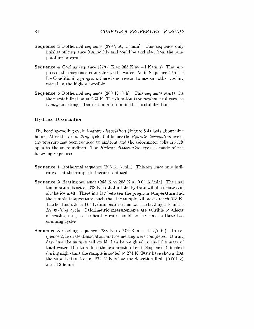
84 CHAPTER 6. PROPERTIES - RESULTS
Sequence 3 Isothermal sequence (279.5 K, 15 min). This sequence only�nishes o� Sequence 2 smoothly and could be excluded from the tem-perature program.
Sequence 4 Cooling sequence (279.5 K to 263 K at �4 K/min). The pur-pose of this sequence is to refreeze the water. As in Sequence 4 in theIce Conditioning program, there is no reason to use any other coolingrate than the highest possible.
Sequence 5 Isothermal sequence (263 K, 3 h). This sequence starts thethermostabilization at 263 K. The duration is somewhat arbitrary, asit may take longer than 3 hours to obtain thermostabilization.
Hydrate Dissociation
The heating-cooling cycle Hydrate dissociation (Figure 6.4) lasts about ninehours. After the Ice melting cycle, but before the Hydrate dissociation cycle,the pressure has been reduced to ambient and the calorimeter cells are leftopen to the surroundings. The Hydrate dissociation cycle is made of thefollowing sequences.
Sequence 1 Isothermal sequence (263 K, 5 min). This sequence only indi-cates that the sample is thermostabilized.
Sequence 2 Heating sequence (263 K to 288 K at 0.05 K/min). The �naltemperature is set at 288 K so that all the hydrate will dissociate andall the ice melt. There is a lag between the program temperature andthe sample temperature, such that the sample will never reach 288 K.The heating rate is 0.05 K/min because this was the heating rate in theIce melting cycle. Calorimetric measurements are sensible to e�ectsof heating rate, so the heating rate should be the same in these twoscanning cycles.
Sequence 3 Cooling sequence (288 K to 274 K at �4 K/min). In se-quence 2, hydrate dissociation and ice melting were completed. Duringday-time the sample cell could then be weighted to �nd the mass oftotal water. But to reduce the evaporation loss if Sequence 2 �nishedduring night-time the sample is cooled to 274 K. Tests have shown thatthe vaporization loss at 274 K is below the detection limit (0.001 g)after 12 hours.

6.3. CALORIMETRIC METHOD 85
Sequence 4 Isothermal sequence (274 K, 5 min). The duration of 5 min-utes is arbitrary. This is just to indicate that the sample is thermosta-bilized at this temperature.
6.3.3 Criticism of the Preliminary Method
Errors in the Preliminary Method
To quantify the errors, the method was used in two experiments. Theseexperiments are called Test 8 and Test 11 in Appendix B. The results aregiven in Table 6.1.
Table 6.1: Experimental results and random errors in calorimeter tests no.8 and 11. For Test 8 the error intervals were calculated using Gauss' law ofrandom error propagation (Levik 1999). For Test 11 the same random errorintervals were assumed. The ideal hydrate number (complete �lling) of sIIhydrate is n = 5:67. The experimental results cover this value.
Test 8 Test 11 Unit
Structure sII sIIn 4:7 � 1:8 4:0� 1:8 -�h�diss 284� 9 315 � 9 J/gf 59� 1 70� 1 %massPproduction 9:0 � 0:5 7:0� 0:5 MPamsample 0:92 � 0:01 0:900 � 0:002 g
The n-intervals covered the ideal hydrate number (5.67), but the relativerandom error in n was about 40%. This error is so large that it makes thepreliminary method of little use in hydrate number determination.
The relative random error in �hdiss was about 3%, which is acceptable.But the values 284 and 315 J/g are about half the dissociation enthalpy of578 J/g estimated from Clausius-Clapeyron calculations (Table 6.2). Thisis an indication that the preliminary method yields a large systematic errorin the dissociation enthalpy measurements.
The relative random error in f is about 1.5% which is satisfactory. Therepeatability in f is not good, but this can be explained by sample inhomo-geneity. The inhomogeneity may be a draw-back of the sampling procedure,but the di�erence in f values is not against the calorimetric method.

86 CHAPTER 6. PROPERTIES - RESULTS
Assumptions Made in the Preliminary Method
Two critical assumptions were made before the development of the prelimi-nary method started:
A big sample which �lls the sample cell can be used. This implied thatthe mass of hydrated gas would be relatively large. Accordingly,weighting would be an easy, direct and accurate way to determinethe mass of the gas. But the tests (Appendix B) showed that if thesample mass exceeded about 0.95 g the logged sample temperature ex-ceeded the hydrate equilibrium curve of the hydrate forming gas. Thiscould not be allowed. A consequence of having to use small sampleswas that the relative random error in ng became large.
Fractionation during hydrate formation is negligible. It was assumedthat the molar mass of the hydrated gas was about the same as themolar mass of the hydrate forming gas. In other words, fractiona-tion was assumed to be negligible. With the knowledge earned later(Chapters 4 and 8) it became obvious that the assumption of negligiblefractionation was unrealistic.
Advances of the Preliminary Method
Handa (1986a) reported work on samples with little free water (ice). Thismethod was tried in the present work without success. This is explainedby complications due to mass transfer between the free water as it melts inthe calorimeter. Despite its shortcomings, the preliminary method was anadvancement towards calorimetric analysis of natural gas hydrate with largeamounts of ice. The preliminary method had three special features:
� Pressurize the NGH-ice sample with methane.
� Apply an ice conditioning cycle before quantifying the ice (Figure 6.5).
� Operate below the methane hydrate equilibrium curve and above theequilibrium line of the hydrate forming natural gas (Figure 6.5).

6.3. CALORIMETRIC METHOD 87
1.65
1.7
1.75
1.8
1.85
260 262 264 266 268 270 272 274 276 278 280T [K]
P [M
pa]
Ice conditioning, heatingIce conditioning, coolingIce melting, heatingIce melting, cooling 273 K
Methane hydrate equilibriumcurve
Natural gashydrate
equilibriumcurve
Figure 6.5: Operation lines in the Ice conditioning and Ice melting cycles.The free water (ice) gives o� absorbed gas around 273 K in the heatingsequence of the Ice condition cycle. This causes a sudden pressure increase.
Since a NGH sample was subject to a pressure exerted by methane, therewere two hydrate equilibrium curves of interest; the curve of the hydrateforming natural gas and the curve of methane. It was necessary that thesample pressure was below the methane hydrate forming pressure to avoidmethane hydrate formation. But the pressure must be high enough to keepthe system above the equilibrium pressure of the natural gas. With theserequirements there would be no formation of methane hydrate since thepressure was too low. There would be no dissociation of methane hydratesince no methane hydrate was there. There would be no formation of sIINGH since the content of ethane and propane in the methane was verylow. There would be no dissociation of the NGH already present since thepressure of methane, which was the major gas component in the hydrate,was too high. This applied to a pressure range de�ned by a temperaturerange, in this case about 263 K to 279 K. In Figure 6.5 it is seen that aninitial pressure of 1.7 MPa was suitable.

88 CHAPTER 6. PROPERTIES - RESULTS
Because of fractionation the NGH equilibrium curve was below the equilib-rium curve of the feed gas. It was therefor conservative practice to operateabove the curve of the feed gas.
The free water was saturated in methane, ethane and propane at appreciablepartial pressures when it froze to ice. Consequently, there was some desorp-tion when this ice melted in the calorimeter under 1.7 MPa methane. Theheat of desorption was registered simultaneously as the heat of ice melting.Accordingly it was not possible to accurately integrate the ice peak. Thusthe Ice conditioning cycle was proposed.
In the Ice conditioning cycle the ice was melted and the water that formedwas allowed to equilibrate with the methane above the sample. The samplewas then brought back to 263 K. It is seen in Figure 6.5 how the pressuresuddenly increases because of desorption at about 273 K during the heatingsequence of the Ice condition cycle. In the next cycle, the Ice melting cycle,the ice melted again. This time the water that formed at 273 K was alreadyequilibrated with the gas. Consequently there was almost no desorptionof gas from the water. The peak was due to melting alone and could beintegrated accurately. The speci�c enthalpy of the melting process weredetermined in separate experiments (Appendix B.2.3, Test 8).
6.3.4 Final Calorimetric Method
An Alternative Approach
It is necessary to modify the preliminary calorimetric method. A newmethod should be devised where a big sample is used. The procedure shouldbe robust towards the composition of the hydrated gas. Two modi�cationsare proposed:
1. In the Ice conditioning and Ice melting cycles, melt the ice isothermallyat 274 K.
2. Measure the pressure increase during hydrate dissociation to determinethe amount (moles) of hydrated gas.
Modi�cation 1 makes it possible to use a big sample which �lls the calorime-ter cell (� 8 cm3). Since the ice melting takes place during isothermal oper-ation the sample temperature will always be above the feed gas equilibriumcurve even if the sample mass exceeds about 0.9 g.
Modi�cation 2 requires that the gas which liberates during dissociationcauses a pressure increase. This increase must be small, thus a gas expan-

6.3. CALORIMETRIC METHOD 89
sion chamber is connected to the calorimeter as in the apparatus of Handa(Figure 2.4). The volume of the whole system (calorimeter cells, expansionchamber and tubing) must be calibrated. The amount (moles) of hydratedgas is calculated using equation 2.8.
Calorimeter Operation
A big sample which completely �lls the calorimeter sample cell will be an-alyzed. Three cycles will be used, just as in the preliminary method. TheIce conditioning and Ice melting cycles are subject to the same change; in-stead of melting the ice during a scanning sequence, the ice is melted duringan isotherm at 274 K. The duration of this sequence will have to be basedon experience. It is also possible to stop the isotherm manually after themelting peak is completed and then cool the sample to complete the cycle.
The Hydrate Dissociation cycle is carried out as in the preliminary method,with the exception that in stead of dissociating in an open system, thesystem is now closed. The gas that liberates during the dissociation causesthe pressure to increase. The pressure increase is measured. Since the systemvolume is calibrated, the amount (moles) of gas can be calculated. Becauseof the expansion chamber the pressure increase is not very large and thesystem is kept in a low pressure region to ensure smooth dissociation. Thisis the principle used by Handa (1986a).
To collect data for cp determination the sample is heated at a constant rateover the temperature interval of interest. Section 6.3.1 describes how cp(T )is found. To �nd cp;hyd it is necessary to subtract the contribution of theice. This can be done since the mass of ice is found and since cp;ice(T ) isknown from Section 6.3.1.
Calculation Procedure
Amount of free water, f (%mass):
f =mice
msample100 (6.1)
where
mice =�H1:7MPa;ice
�h1:7MPa;ice(6.2)

90 CHAPTER 6. PROPERTIES - RESULTS
The subscript 1:7 refers to the methane pressure 1.7 MPa during the icemelting process.
Hydrate number, n (-):
n =nw;hydng
(6.3)
wherenw;hyd = nw;tot � nice =
mw;tot
Mw� nice (6.4)
and ng is found by equation 2.8:
ng =(Pf � Pi � Pw)(Vt � Vw)
RTg +B(Pf � Pi � Pw)
To �nd the volume average of the gas temperature, Tg, an extension ofequation 2.9 is suggested; equation 6.5. It includes a contribution from thereference cell, since the reference cell contributes to the total system volume.
Tg =V1Tr +
12V2(Tc + Tr) + Tc(VS � Vw) +
12V
0
2 (Tc + Tr) + TcVR
Vtot � Vw(6.5)
where V0
2 corresponds to V2 except the latter is for the sample cell and the�rst for the reference cell. The rest of the symbols are the same as forequation 2.9.
Speci�c enthalpy of hydrate dissociation, �hdiss (J/mol):
�hdiss =�Hdiss
ng(6.6)
Speci�c heat capacity, cp (J/gK), is found according to the procedure de-scribed in Section 6.3.1.
cp =d�H(T )
dT
=d
dT(a+ a0T + a1T
2 + a2T3 + � � � + an+1T
n)
= a0 + a1T + a2T2 + a3T
3 + � � � + anTn (6.7)

6.4. PROPERTIES ESTIMATES 91
6.4 Properties Estimates
To estimate thermophysical and compositional properties of natural gas hy-drate, the models and correlations found in the literature (Chapter 2) wereused. The calculations and assumptions are given in Appendix C. Theresults are collected in Table 6.2.
Table 6.2: Estimated thermophysical and compositional properties of sIInatural gas hydrate.
Property Value Remark
C1:C2:C3 89:6:5 %mol assumptionn 6 assumptionMNG 18.24 g/mol�h�diss 73.0 kJ/mol Clausius-Clapeyron�h�diss 578 J/g =(73 kJ/mol)�1000=(MNG + 18n)cp 2.28 J/gK (Groisman 1985)cp 287 J/molK =(2.28 J/gK)�(MNG + 18n)� 0.373 W/Km for �=700 kg/m3, (Groisman 1985)dl=ldT 52 � 10�6 K�1 (Sloan 1998, p.64)
6.5 Discussion
6.5.1 Calorimetric Method
Most literature report how �hdiss, n and f are found for single-guest hy-drates with very low ice content. This work focuses on analyses of multi-guest hydrates with very high ice content. Handa (1988b) reported analysison a natural gas hydrate sample with ice (NGH8 in Table 2.2). It was notpossible to determine the ice contents of this sample. Consequently, n and�hdiss could not be determined either. If all cages in NGH8 were occupied,then it contained about 20 %mass of ice. Full occupancy is not possible, sothe ice content must have been below 20 %. To compare, the samples in thepresent work contained about 40-70 %mass ice.
The contribution of the present work is to expand Handa's method (Handa1986a) to make it more suitable for samples of mixed hydrates with largeamounts of ice. From the calorimeter tests (Appendix B) it was concludedthat the heat of ice melting depends on the pressure at which the ice formed,

92 CHAPTER 6. PROPERTIES - RESULTS
the pressure at which the ice is melted and the composition of gas used topressurize the ice during the analysis. More speci�cally; when ice froze under6-9 MPa natural gas and melted under a 1.7 MPa methane, processes tookplace that had a thermal response. Two processes could be important: des-orption of natural gas and PV work. It was not possible to make meaningfulcorrections for these e�ects. E�ects related to the presence of hydrate areless likely, since similar e�ects were seen in water-nitrogen systems withoutany hydrate (Appendix B.2.2).
To get around the complications that arose from desorption, it was suggestedthat the calorimeter method should have an extra heating-cooling cycle be-fore the actual analysis. The purpose of this extra cycle is to condition orpretreat the sample, or actually the ice in the sample. This was achievedby melting the ice at a suitable pressure and allowing the water to equili-brate with the gas and then refreeze the water. This cycle was called the Iceconditioning cycle. Then, during the Ice melting cycle the ice melted undera gas with which it was equilibrated at the PT conditions at the meltingpoint. The speci�c enthalpy of ice melting for these conditions were foundin separate experiments. Then the mass of free water in the sample couldbe calculated.
It was also concluded from the tests that to pressurize the sample with thehydrate forming natural gas introduced errors because of a complicated andnot fully understood thermal response around the melting point. Hydrateformation seemed to take place. Instead of pressurizing with natural gas itwas decided to pressurize with methane. A suitable pressure, as mentionedabove, was a pressure below the hydrate curve of methane and above thehydrate curve of the hydrate forming gas. For the temperature interval ofinterest, 1.7 MPa was a suitable pressure, as illustrated in Figure 6.5.
Getting around the problems associated with the high ice content in this way;pressurizing natural gas hydrate with methane and operating between thecorresponding equilibrium curves, is one of the main results of the presentwork. It is also suggested that the Ice melting cycle includes an isothermat 274 K. It must last long enough for all ice to melt. This will allow largesamples and the random errors will be reduced accordingly.

6.5. DISCUSSION 93
6.5.2 Hydrate Sampling
In this section it is suggested why �ltration of hydrate-in-water slurries isso di�cult. It is then proposed how �ltration could be carried out.
Filtration Mechanism
Hydrate was separated from the hydrate-in water slurries by inline �ltration.The samples that were obtained contained large amounts of free water. Fil-tration of hydrate slurries is known to be di�cult. It is di�cult to grow largehydrate crystals with good �ltration characteristics. Light, feathery crystalswhich form compacted beds are quite common (Mullin 1994, p.360). Thesame behavior was observed in numerous hydrate production and �ltrationexperiments.
The poor �ltration properties could be explained if there is no build-up ofa proper �lter cake. What happens instead is perhaps the build-up of ahydrate plug in the �lter. This hypothesis is based on the fact that the�lter cloth more or less resembles a hydrate plug; a stationary ow restric-tion. The slurry will continue to build the \plug" (the �lter cloth) alreadythere. Accordingly, the material that �lls the �lter cup will have similari-ties to hydrate plugs. For example, the water content may be very high, asmeasured in the present work. Filtration is then a way of collecting plugsamples. Therefor this work becomes relevant for plug related topics. Forexample, the plug dissociation characteristics, which are intimately relatedto the thermophysical and compositional properties, are important in owremediation.
Washing Agent
It may be possible to remove the water in the �lter cake by some washingagent. The washing agent will have to meet these criteria:
� It must be a water soluble liquid.
� It must be volatile for temperatures well below 273 K.
� It must be sub-critical at pressure-temperature conditions at the hy-drate process.

94 CHAPTER 6. PROPERTIES - RESULTS
� It should not be a hydrate former.
� It must not have a destabilizing e�ect on the hydrate.
It is suggested that 1-butanol may be used. But since 1-butanol is a hydrateinhibitor, its e�ect on the hydrate stability may be undesirable. It meetsthe other criteria. The idea is that after �ltration the �lter is ushed with1-butanol at the operating pressure and temperature. In theory, the waterin the �lter will gradually be replaced by the alcohol. In the end the alcoholcould be displaced by gas in the ordinary and proven manner. Then the�lter is cooled to about 250 K to stabilize the hydrate. When the �lter isopened the cake will be pasty instead of solid and ice-like. The paste isspread in a thin layer at about 250 K and left for the alcohol to evaporate.The remaining product will be dry, pure hydrate.
6.6 Conclusions
� A calorimetric method was developed for analyzing natural gas hydratethat contain large amounts of free water (ice). The advances comparedto previous works are:
1. Natural gas hydrate is pressurized with methane and the systemis operated at PT -conditions that are below the methane hydratecurve and above the natural gas hydrate hydrate curve.
2. In a sample conditioning step the ice is equilibrated with the gasused to pressurize the sample.
� Standard hydrate dissociation enthalpy was measured. The valueswere lower than expected.
� Hydrate number was measured. The relative error was large.
� Free water was measured. The values were reasonable and errors wereregarded acceptable.
� Improvements of the method was suggested to reduce the errors indissociation enthalpy and hydrate number.
� Speci�c heat capacity for ice was �tted as a virial equation in T . Thecorrespondence to literature measurements was good.cp;ice = 6 � 10�5T 2 + 0:0108T + 2:1187 for �34 �C < T < �1 �C.

Chapter 7
Metastability - Results
7.1 Introduction
The �rst purpose of the work reported in this chapter was to develop calori-metric methods to quantify metastability of natural gas hydrate. An isother-mal method can be used to measure the rate of very slow dissociation pro-cesses. It quanti�es how (if) the amount of natural gas hydrate changesduring storage.
The second purpose of the work reported in this chapter was to develop aclimate laboratory where the storage conditions could be controlled. Thestorage apparatus is described in Chapter 5.5.
7.2 Isothermal Calorimetry Method
There was no evidence found in the literature (Chapter 3) that metastablehydrate can exist inde�nitely. Accordingly, it was assumed that metastabil-ity properties of hydrate can be described in terms of kinetic metastability ;the sample undergoes steady dissociation, but the rate of dissociation is solow that the hydrate persists for long times. It follows that metastabilitycan be quanti�ed by the rate of dissociation, which in turn can be correlatedto storage conditions and sample characteristics. An isothermal calorimetricmethod based on the principles outlined in Section 3.4 was developed.
The sample was transferred to the calorimeter as described towards the end
95

96 CHAPTER 7. METASTABILITY - RESULTS
of Section 6.2. Since the calorimeter was operated in isothermal mode, itcould be said that the samples were stored in the calorimeter at well de�nedand constant pressure and temperature. After the initial thermostabiliza-tion, a steady heat ow signal, _Q (W), was collected. The signal was weakdue to the very low rate of dissociation. The signal was corrected by sub-tracting the blank signal, or else a relatively large error would result. Thecollected signal, _Q (W), was referred to the initial sample mass to �nd thespeci�c heat ow, _q (W/g). By convention, a negative heat ow correspondsto heat ow to the sample.
The procedure was tested in two series of experiments. Temperature (T )and sample diameter (D) were the independent variables.
7.2.1 E�ect of Temperature
The results from the temperature e�ect experiments are shown in Figure 7.1.Three experiments were done at temperatures of 272, 268 and 238 K usingparticles with D � 1 mm. A high temperature gave a large heat ow to thesample, and the dissociation rate was relatively high. It was also seen thatthe collected heat signals at 268 and 238 K were fairly constant, except they uctuated somewhat. This indicated constant rates of dissociation. Theheat signal collected at 272 K varied more.
The data in Figure 7.1 provided a basis for estimating the rate of dissocia-tion. It was necessary to estimate the amount of free water in the samples.It had been found in previous experiments that f = 40 %mass was a reason-able assumption. The correlation �hdiss = 215:59 � 103 � 394:945T (J/kg)for 248 K < T < 273 K (Selim and Sloan 1990) was used to �nd �hdiss. ForT = 268 K the correlation yields 110 J/g. The rate of hydrate dissociationwas calculated using the relation
rdiss =�3600 _q
0:4�hdiss(7.1)
where the constant 0.4 is due to the assumption that f = 40 %mass. It isalso useful to put a number on the degree of conversion or dissociation, �,after a time interval of interest, for example 240 hours (10 days). If rdissremains constant, then _q remains constant, and then

7.3. DISCUSSION 97
� =� _qt
�hdiss(7.2)
Results from rdiss and � calculations are presented in Table 7.1.
Table 7.1: Quanti�cation of NGH metastability. �240h values are extrapo-lations.
Sample T (K) D (mm) � _q (mW/g) rdiss (1/h) �240hGranulate 238 � 1 > 0 - -Powder 268 < 1 �0:035 0.0029 0.27Granulate 268 � 1 �0:014 0.0011 0.11Granulate 268 � 10 �0:027 0.0022 0.21Granulate 272 � 1 �0:25 0.020 1
7.2.2 E�ect of Sample Diameter
The e�ect of diameter (D) is shown in Figure 7.2. Three experiments werecarried out on particles with diameters of < 1 mm, � 1 mm and � 10 mmat a temperature of 268 K. No correspondence between D and _q was found.The data were corrected by subtracting blank data obtained at 268 K. rdissand � values are presented in Table 7.1.
7.3 Discussion
7.3.1 Rate Limitations
An important issue regarding kinetic metastability is to determine if the raterepresents intrinsic kinetics, or if the rate is limited by heat or mass transferprocesses. During the isothermal calorimetric experiments the calorimeterwas operated at a de�ned temperature set point. Due to dissociation, aheat ow in the order of magnitude 0.1 W was supplied by the calorimeterto maintain the temperature setpoint. In other words, the heat was suppliedas a consequence of dissociation. An adiabatic system would probably self-cool to a lower temperature, as observed by Ershov and Yakushev (1992).
The calorimeter may supply heat ows of about 0.5 W which is about 5 timesthe heat ow in the experiments. This makes it unlikely that rate limitations

98 CHAPTER 7. METASTABILITY - RESULTS
-0.5
-0.4
-0.3
-0.2
-0.1
0
0.1
0 5 10 15 20 25
t [h]
q [m
W/
g]
.
272 K 268 K 238 K
Figure 7.1: E�ect of temperature on NGH metastability. D � 1 mm.
-0.5
-0.4
-0.3
-0.2
-0.1
0
0.1
0 5 10 15 20 25
t [h]
q [m
W/
g]
. Granulate, ~1 mm Granulate, ~10 mm Powder, <1 mm
Figure 7.2: E�ect of sample diameter on metastability. T = 268 K.

7.3. DISCUSSION 99
are due to limitations in the heat transfer. There were large amounts of icein the system. As suggested in the literature, the ice could make it di�cultfor the gas to escape. Consequently, the dissociation rate could be limitedby mass transfer.
7.3.2 E�ect of Temperature and Sample Size
The isothermal method was tested in too few experiments to develop mean-ingful correlations and to quantify the errors. However, when rdiss valuesare plotted (Figure 7.3) to illustrate the combined e�ects of D and T , itseems clear that the temperature e�ect is much more pronounced than thediameter e�ect, in the D and T ranges used here.
238268
272
<1
~1
~10
0
0.002
0.004
0.006
0.008
0.01
0.012
0.014
0.016
0.018
0.02
rdiss [1/h]
T [K]
D [mm]
Figure 7.3: Combined e�ect of temperature and diameter on dissociationrate.
If the three experiments at 268 K are compared, there seems to be no corre-spondence between sample size and the dissociation rate. From D < 1 mmto D � 1 mm the rate decreased from 0.0029h�1 to 0.0011h�1. This was

100 CHAPTER 7. METASTABILITY - RESULTS
expected. But increasing D further, from � 1 mm to � 10 mm, caused therate to increased to 0.0022. This was not expected. It is not known whetherthe deviating behavior is due to random error or sample inhomogeneities.The latter seems more likely, since to determine rdiss it was assumed that allsamples contained 40 %mass free water (ice). This assumption could easilycause errors of 10% or more in the rdiss values.
Despite the inaccuracies, the results seemed reasonable. For D � 1 mm,at 268 K the estimated degree of conversion (�) after 10 days was only0.11 while at 272 K the sample was completely dissociated by this time. Itwas con�rmed that even at a relatively high temperature of 268 K, naturalgas hydrate has metastability properties that justi�es further work with thehydrate process for storage and transport of natural gas.
7.3.3 E�ect of Pressure
The isothermal method can be used at any pressure, for example ambientpressure when using calorimeter cells that are open to the surrounding at-mosphere. In the experiments reported here, closed cells were used, andaccordingly the pressure increased as more and more hydrate dissociated.
The e�ect of the gauge pressure on the dissociation rate was insigni�cant.This is evident since the _q curves are about at if the uctuations are ig-nored. If the increasing pressure had caused a shift (decrease) of the dissoci-ation rate, this would have been re ected in a proportional shift in _q whichwould approach zero. But on the contrary, the only experiment with a shift(T = 272 K, D � 1 mm) showed an unsteady increase in the dissociationrate.
The fact that the e�ect of temperature on the dissociation rate is as ex-pected, further supports that there was no signi�cant e�ect of the gaugepressure on dissociation rate in these experiments. But it should be notedthat if an experiments last signi�cantly longer than in this work, the gaugepressure will have an e�ect, according to theory.
7.3.4 Blank Run
Experiments were carried out at 272, 268 and 238 K. All _q data were cor-rected by subtracting a blank run carried out at 268 K. The resulting curvefor 238 K was disregarded, since it showed a positive value, _q � +0:05 mW/g

7.3. DISCUSSION 101
(Figure 7.1). This could at a �rst glance be taken as an indication of hydrateformation, but that was not possible. A likely explanation is that the blanksignal recorded at 268 K over compensated the measurements at 238 K.
A similar type of over compensation, but oppositely directed and smaller,was probably encountered in the curve for 272 K. This error is assumedinsigni�cant. To obtain better accuracy the blanks should be run at thesame temperature as the corresponding experiments, but there was onlytime to do one blank (268 K).
7.3.5 Micro Regimes
An important visual observation was made on the hydrate samples from thefractionation laboratory. Small, white regions sometimes developed insidethe samples. The hypothesis is set forth that this was caused by the forma-tion of small gas bubbles around hydrate agglomerates which partially dis-sociated to gas and ice. This would create micro regimes where the pressurewas higher than the ambient, perhaps as high as the equilibrium pressureat the storage temperature.
The consequence is that the hydrate inside the samples is subject to storageconditions that favor long-time storage. It may be that a large fraction of thehydrate was subject to conditions at or close to phase equilibrium, even if thebulk material is stored at ambient pressure. The formation of an ice layeron the sample surface has been observed and is reported in the literature(Chapter 3). But no reports describing the experimental observation of gasbubbles inside the samples were found.
Raman spectroscopy could perhaps be used to study this further. It maybe that the signals from hydrated guests gradually decrease, while the sig-nals from ex-guests in small gas bubbles gradually increase. Eventually thesignals may even out due to enhanced hydrate stability resulting from thepressure exerted by the gas in the bubbles.
7.3.6 Other Comments
The heat signal for the experiment at 272 K showed larger uctuations thanthe others. This could be so because the system was close to the ice meltingpoint, so the ice became less able to stabilize the hydrate. It could also bethat sample inhomogeneities gave the large uctuations as zones with more

102 CHAPTER 7. METASTABILITY - RESULTS
or less hydrate dissociated. This is to rely on the hypothesis that the icestabilizes the hydrate.
The three-cycles method proposed in Section 6.3.4 can be used to �nd thehydrate number. First, a fresh sample is analyzed to �nd the hydrate numberto have a reference value. Then, samples are subject to metastable storageat controlled conditions (temperature, relative humidity) in the climate lab-oratory. Finally, the stored samples are analyzed to �nd the hydrate numberafter storage. The hypothesis is that the changes in the hydrate number arenegligible during storage of hydrate. This is likely, since the escape tendencyof guest molecules is extremely low when they are not liberated at the sur-face of a dissociating sample. The guest would have to escape from its cage,di�use through the hydrate phase and perhaps through some ice too. Thisprocess is negligible for all practical purposes.
7.3.7 Speculations on Metastability
Metastability of natural gas hydrate is not well understood, although a num-ber of authors propose (Section 3.2) that an ice layer forms on the sampleand inhibits the dissociation process. In the following it is suggested how asolid mixture approach may be useful in understanding hydrate metastabil-ity.
Metal alloys that are quenched rapidly may consist of many phases in a solidmixture. Such phases are often thermodynamically unstable but persistbecause they are metastable. To pursue this approach it may be useful toconsult the metallurgic and solid materials literature, notably Adams andKaufman (1997), Gaskell (1994) and Godreche (1992). It is also knownthat if two polymer solutions are mixed and the solvent evaporated, thena polymer mixture forms that may be thermodynamically unstable. Themixture may persist because the polymer chains are sterically �xed. Thepolymer mixture is metastable.
The analogy to frozen hydrate with free water (ice) is that the two phasesmake a solid mixture too. It may be that if an unstable phase (hydrate)is caught in a matrix of a stable phase (ice), this promotes metastable be-havior of the unstable phase. Hypothesis: Metastability of NGH is due tostabilization by a thermodynamically stable ice matrix. This implies that acertain amount of free water (ice) is necessary to obtain metastability.
7.4. CONCLUSIONS 103
The resemblance to the ice layer theory in the literature is obvious. An icelayer or an ice matrix is in e�ect the same; a barrier between the hydrateand the surrounding gas phase. The di�erence is that the ice layer formswith time as a portion of the hydrate dissociates. The ice matrix is originallythere and no initial dissociation is required. In popular terms, the price topay for stabilization by an ice layer is the gas that initially evolves. Thisgas is lost or requires handling. The price for stabilization of an ice matrixis a reduced bulk gas content compared to pure hydrate.
7.4 Conclusions
� An isothermal calorimetry method was developed to study metasta-bility of natural gas hydrate with ice for temperatures below 273 K.
� Metastability of natural gas hydrate with ice was demonstrated at268 K.
� Rate of dissociation decreases with decreasing temperature.
� Rate of dissociation seems to be limited by mass transfer.
� Visual observations indicated that gas bubbles may form inside thesamples to create micro-regimes of elevated pressure. This may havean e�ect on the stability of the hydrate.

104 CHAPTER 7. METASTABILITY - RESULTS

Chapter 8
Fractionation - Results
8.1 General Fractionation Model
A general fractionation model, including a functional relation between frac-tionation and the driving force (subcooling), is proposed. It is based onthree hypotheses:
H1 When operating with zero driving force (on the equilibrium line), thelargest possible fractionation takes place.
H2 When operating with in�nite driving force, no fractionation takes place.
H3 Between these extremes, the fractionation as function of the drivingforce changes exponentially.
It is not practicable to operate a system on the equilibrium line (H1). Theexact position of any equilibrium line is unknown. Even if it was exactlyknown, it would be necessary to have pressure and temperature regula-tion with zero error bands, which is impossible. In the apparatus used inthis work, the composition of the gas in the reactor changes as propane isdepleted and methane is being enriched. Consequently, the hydrate equi-librium line of the gas shifts upwards in the pressure-temperature plane. Itfollows that the system behavior at the boundary where the driving force iszero can not be determined experimentally. The best thing that can be doneis to do experiments with small, yet signi�cant, driving forces (�T = 2K).
105

106 CHAPTER 8. FRACTIONATION - RESULTS
Consequently, at the boundary where the driving force is zero, the assump-tion above (H1) has to be made.
It is impossible, indeed without any physical meaning, to do experimentswith in�nite driving force (H2). For an equilibrium temperature Teq, thehighest practical driving force in the apparatus used is �T = Teq � 273. Alarger driving force would bring the system below 273 K where the waterfreezes to ice. The best thing that can be done is to do experiments close to,yet above, 273 K. For an in�nite driving force the assumption above (H2)has to be made. Following this line of thought, complete suppression offractionation is not possible in practical operations.
The functional relation (H3) between fractionation and the driving forcemust be consistent with H1 and H2. Thus, the content of any componentin the hydrate as the driving force (�T ) approaches zero is the equilibriumcontent, Ci;eq (H1). This value follows from the theory of Section 4.1.2,and can be calculated using CSMHYD (Sloan 1998), for example. Whenthe driving force approaches in�nity, the composition of the hydrate gasapproaches the composition of the feed gas, which is known (H2).
It follows that the functional relation for fractionation starts at a �nitevalue between 0 and 100 %mol for �T = 0, and approaches the feed gascomposition asymptotically for increasing driving forces. An exponentialterm is assumed to describe this behavior.
Fractionation is known to be component dependent and pressure dependent.It is believed to be system dependent too. Accordingly, the function mustcontain a system dependent empirical constant, k(P; i). For a system withn guests, exponential expressions are deduced for n � 1 guests. The lastequation is the mass balance which closes at 100 %mol. For the system inthe present work with methane, ethane and propane as guests, the threehypotheses can now be formulated in mathematical terms:
H1 Ci;diss = Ci;eq = �i;eq � 100 �T = 0H2 Ci;diss = Ci;feed �T =1
H3-a Ci;diss = (Ci;feed � Ci;eq)e�k(P;i)=�T + Ci;eq 0 < �T <1, i = C1, C3
H3-b CC2;diss = 100 � (CC1;diss + CC3;diss) 0 < �T <1, i = C2
The most important equation is the one labeled H3-a. It expresses how thehydrate content of guest type i depends on the content of guest i in the feedgas, pressure and driving force. This equation contains equations H1 and H2;

8.2. METHODS 107
Equation H3-a yields Ci;eq for �T = 0, as in Equation H1. Equation H3-ayieldsCi;feed for �T =1, as in Equation H2. Ci;eq in Equation H3-a is equalto �i;eq � 100, and when �i;eq is substituted using equation 4.3, Equation 8.1results. To completely write out the equation calls for further substitutionsusing the equations in Section 4.1.2.
Ci;diss =
0@Ci;feed � 100
16�s;i + 8�l;i
16P
i �s;i + 8P
i �l;i
!eq
1A e�k(P;i)=�T + Ci;eq
(8.1)
8.2 Methods
The purpose of this work was to investigate the e�ect of driving force onfractionation, notably to evaluate the suitability of the proposed fractiona-tion model. To accomplish this, the driving force was varied by operatingat di�erent pressures and temperatures. The driving force was expressed interms of subcooling relative to the hydrate equilibrium curve for the feedgas. The experiments can be grouped in terms of driving force. 2, 4, 8, 12and 16 K subcooling were used. Experiments can also be grouped in termsof operation pressure. 3.0, 4.5, 6.0 and 7.5 MPa were used. With these setsof driving forces and operating pressures, a set of operating temperatures isimplicitly de�ned.
Figure 8.1 shows the CSMHYD equilibrium curve for the feed gas and thecurves for the planned driving forces. The operation points lie where thecurves for the planned driving forces intercept the planned isobars. Eachexperiment was numbered as shown in the �gure.
The apparatus was described in Section 5.6. To produce hydrate, distilledwater (80 cm3) was brought in contact with natural gas (5 %mol ethaneand 3 %mol propane in methane). But before feeding the gas, the air in thereactor and air that was dissolved in the water was removed by evacuatingthe reactor (�5 Pa) for 20 minutes or more. Then the reactor was cooledto the operating temperature, while pressurized with the gas to somewhatbelow the equilibrium pressure for this temperature. The magnetic stirrerwas started (about 400 RPM). When the desired temperature was reached,the data logger was started and the reactor pressurized to the operatingpressure. The reactor was operated for about four hours. The pressure-

108 CHAPTER 8. FRACTIONATION - RESULTS
0
1
2
3
4
5
6
7
8
9
10
273 274 275 276 277 278 279 280 281 282 283 284 285 286 287 288 289 290 291 292 293
T [K]
P [M
Pa]
∆T=16 K ∆T=12 K ∆T=8 K ∆T=4 K ∆T=2 K
Equilibrium
1 2, 2rep3 4
86, 6rep6repA 5
910
11
12 13
14 1516
Figure 8.1: Plan for the fractionation experiments. The equilibrium curveis for a gas with ethane (5 %mol) and propane (3 %mol) in methane and iscalculated using CSMHYD (Sloan 1998).
temperature course during an experiment (no. 2, P=7.5 MPa, T=287 K,�T=4 K) is illustrated in Figure 8.2. Afterwards, a sample of the gas inthe reactor was analyzed by gas chromatography. The results are reportedas Ci;reac in Tables 8.1 to 8.4. Then the reactor was refrigerated (252 K)overnight. Note that due to fractionation, the composition of the gas phasein the reactor changed during the experiments. This is discussed later.
The next day the reactor was quickly depressurized to ambient pressure. Ittook about half a minute or less, depending on the initial reactor pressure.The reactor was opened, and hydrate quickly scraped into the precooleddissociation cell. The cell was closed immediately. The sample transfer tookplace in the freezer at around 252 K.

8.3. MEASUREMENTS 109
0
1
2
3
4
5
6
7
8
9
10
273 274 275 276 277 278 279 280 281 282 283 284 285 286 287 288 289 290 291 292 293
T [K]
P [M
Pa]
Equilibrium
∆T = 4 K
Figure 8.2: Pressure-temperature course during experiment no. 2 withP=7.5 MPa and �T=4 K. The cluster of data points around the PT setpoint contains about 450 measurements collected during nearly 4 hours.
8.3 Measurements
Tables 8.1 to 8.4 give the results of all the gas chromatograph measurements.Ci;reac (%mol) is the content of gas i in the reactor when the hydrate pro-duction was stopped after 4 hours operation. Ci;diss (%mol) is the content ofgas component i in the gas from a completely dissociated sample. Ci;reac andCi;diss were normalized to 100 %mol. A three dimensional plot illustratesthe combined e�ects of driving force and pressure on methane fractionation(Figure 8.3).

110 CHAPTER 8. FRACTIONATION - RESULTS
Table 8.1: Composition of reactor gas and gas from dissociated samples.Hydrate production pressure was 7.5 MPa.
Ci;reac (%mol) Ci;diss (%mol)Run no. �T (K) CH4 C2H6 C3H8 CH4 C2H6 C3H8
4 2 93.4 4.6 2.0 76.6 10.1 13.24 2 76.0 9.6 14.42 4 94.5 4.1 1.4 85.6 6.9 7.62 4 84.8 7.4 7.82rep 4 93.2 4.5 2.3 75.6 9.3 15.13 8 92.5 4.8 2.7 85.1 7.5 7.41 16 92.2 5.0 2.9 88.9 6.0 5.1
Table 8.2: Composition of reactor gas and gas from dissociated samples. Su-perscript � indicates gross errors. Hydrate production pressure was 6.0 MPa.
Ci;reac (%mol) Ci;diss (%mol)Run no. �T (K) CH4 C2H6 C3H8 CH4 C2H6 C3H8
7 2 92.4 4.9 2.8 83.5 6.8 9.75 4 93.1 4.5 2.4 76.8 10.7 12.56 8 *90.8 *5.4 *3.8 84.4 7.7 7.96rep 8 92.7 4.8 2.6 84.6 7.8 7.66repA 8 92.6 4.8 2.7 84.3 7.9 7.76repA 8 84.0 8.0 8.011 12 92.2 5.0 2.8 88.4 5.9 5.611 12 92.1 5.0 2.98 16 92.3 4.9 2.8 89.3 5.6 5.18 16 89.5 5.6 5.0
Table 8.3: Composition of reactor gas and gas from dissociated samples.Hydrate production pressure was 4.5 MPa.
Ci;reac (%mol) Ci;diss (%mol)Run no. �T (K) CH4 C2H6 C3H8 CH4 C2H6 C3H8
9 2 93.1 4.8 2.1 76.1 8.9 15.013 4 93.4 4.5 2.1 76.6 10.2 13.310 8 92.9 4.7 2.4 82.4 8.4 9.212 12 92.4 4.9 2.7 89.0 5.6 5.412 12 88.9 5.6 5.5

8.3. MEASUREMENTS 111
Table 8.4: Composition of reactor gas and gas from dissociated samples.Hydrate production pressure was 3.0 MPa.
Ci;reac (%mol) Ci;diss (%mol)Run no. �T (K) CH4 C2H6 C3H8 CH4 C2H6 C3H8
16 2 93.3 4.7 2.0 73.0 9.3 17.715 4 94.7 4.1 1.2 75.5 10.7 13.814 8 93.9 4.3 1.8 79.3 9.6 11.1
24
812
16
3
4.5
6
7.5
70
72
74
76
78
80
82
84
86
88
90
CC1,diss
∆T [K]
P [Mpa]
Figure 8.3: Concentration of methane in gas from dissociated hydrate sam-ples as function of operation pressure and driving force. The plot illustratesthat driving force and pressure should be high to suppress fractionation.

112 CHAPTER 8. FRACTIONATION - RESULTS
8.4 Interpretation of Measurement Results
8.4.1 Driving Force Threshold
Hypothesis
Earlier observations made in the NTNU Hydrate Laboratory indicated thatthere is a connection between the hydrate formation conditions and thehydrate composition. Hypothesis:
� There exists a driving force threshold beyond which the fractionationis insigni�cant.
Findings
It is known that fractionation occurs for small driving forces. Thus, tocheck the hypothesis, it was necessary to do only one experiment using thelargest driving force possible. If insigni�cant fractionation was observed,then the hypothesis could be regarded true. But if signi�cant fractionationwas observed, the hypothesis needed not be regarded false. It would onlymean that with the available apparatus it was not possible to achieve adriving force large enough to suppress fractionation.
The largest driving force that could be obtained was 17 K subcooling. How-ever, the largest subcooling used in the experiments was 16 K. It was as-sumed that this relatively small di�erence of 1 K had no impact on theconclusion regarding a driving force threshold. Two experiments were car-ried out with 16 K subcooling; experiment no. 1 (P=7.5 MPa, T=275 K)and no. 8 (P=6.0 MPa, T=273.5 K), see Tables 8.1 and 8.2. Fractionationwas observed in both experiments. The hydrate produced in experimentno. 1 had a normalized methane content of 88.9 %mol which is a reductionof 3.1 %mol compared to the feed gas with 92 %mol methane. The gasfrom the dissociated hydrate contained 5.1 %mol propane, while the feedgas contained 3 %mol. For experiment no. 8 the �gures were about thesame. The hypothesis of insigni�cant fractionation for large driving forcesremains unsupported.

8.4. INTERPRETATION OF MEASUREMENT RESULTS 113
8.4.2 System Speci�c Fractionation Model
Generally, the average reactor gas composition, Ci;reac, was taken as the av-erage of the initial reactor gas composition and the �nal reactor gas compo-sition. In symbols: Ci;reac = (Ci;feed+Ci;reac)=2. H1 applies when �T = 0,and there are no Ci;reac values available in this case. Ci;reac values have tobe estimated. This is done graphically in Figures D.1 and D.2 for methaneand propane, respectively. The estimation for ethane follows from the massbalance;
PCi;reac = 100 %mol. Ci;reac and CCSMHYD
i;eq values for �T = 0are given in Table 8.5.
Table 8.5: Average composition of the gas in the reactor (Ci;reac) for�T = 0 as found in Figures D.1 and D.2, and simulated composition ofthe corresponding equilibrium hydrate (CCSMHYD
i;eq ). Values are normalizedto 100 %mol. These are estimates, and the many decimals are not signi�cantbut are given here for traceability. Average ethane content of the reactorgas is CC2;reac = 100 � (CC1;reac + CC3;reac).
Ci;reac (%mol) CCSMHYDi;eq (%mol)
P (MPa) CH4 C2H6 C3H8 Sum CH4 C2H6 C3H8 Sum
7.5 92.825 4.600 2.575 100 69.13 3.63 27.24 1006.0 92.825 4.600 2.575 100 68.00 3.52 28.48 1004.5 92.950 4.650 2.400 100 66.93 3.61 29.46 1003.0 93.775 4.425 1.800 100 66.26 4.10 29.63 99.99
As seen in Figures D.1 and D.2, the reactor gas composition data for �T = 2 Kdeviate from the pattern established by the other data. The same obser-vation is made for the hydrate composition data in Figures 8.5 and 8.6.Three important questions arise. The questions must be treated in the fol-lowing order and they must be treated at this point, since the answers haveconsequences for the fractionation modeling.
� Are the deviations signi�cant?
� How can the deviations be explained?
� Should the deviating data have in uence on the k-values?
Answers to these questions are proposed in the following. Data points inFigures 8.4 to 8.7 show that for �T > 4 K fractionation is suppressed if �T

114 CHAPTER 8. FRACTIONATION - RESULTS
is increased. But a less clear (Figure 8.6) or even contradicting (Figure 8.5)behavior is seen in that a driving force of 2 K may cause less fractionationthan a driving force of 4 K. Figure D.2 shows that for 3.0 MPa operationpressure, the reactor gas at the end of experiments is richer in propane for�T = 2 K than for �T = 4 K and also for �T = 8 K. This is noteworthy,even if the hydrate composition did not deviate form the overall trend inthis case. A similar pattern was seen for methane at 3.0 MPa. On thisbackground, the deviations for �T = 2 K are regarded signi�cant.
It is observed that as the driving force becomes smaller than 4 K, thenfractionation may be suppressed compared to larger driving forces. This iscontrary to expectations. The behavior may be explained by kinetic e�ects.In case of a small driving force, about 2 to 4 K and smaller, the degreeof conversion is low due to a long induction time (stochastic) and a lowgas consumption rate (deterministic). Consequently little gas is (may be)consumed, which implies a small change in the gas composition. Followingthis line of though, at the limit of zero driving force there would be nogas consumption. Then the gas composition at the end of an experimentwould be equal to the feed gas composition, and no fractionation would beobserved. But this is only because the system does not reach equilibriumduring the four hours the experiments last. This behavior is likely to behighly apparatus dependent. On this basis the deviating data for �T = 2 Kare not processed further and has no in uence on the model. The data pointsare labeled \&" in Figures 8.4 to 8.7. This line of though is supported by theexperimental results of Khokhar (1998) who found that when the drivingforce (subcooling) was increased 47% the water conversion increased up to450%. A summary of the three answers is then:
� The deviations at �T = 2 K are signi�cant.
� The deviations are explained by kinetic phenomena.
� The deviating data are not given in uence on the modeling.
k-values were determined for methane and propane. Least squares plots withP(model(k;�T )�data(�T ))2 on the ordinate and k on the abscissa were
made for each pressure (Figures D.3 to D.10, page 159). k(P; i) was readfrom these plots. The procedure was repeated eight times (8=2x4, 2 com-ponents and 4 pressures). Expressions for CC1;diss and CC3;diss could thenbe written out explicitly for each pressure (Table 8.6). The same procedure

8.4. INTERPRETATION OF MEASUREMENT RESULTS 115
could be used for ethane, but then the mass balance would in general notclose at
PCi;diss = 100 %mol. To achieve this, the content of ethane in
the hydrate was instead found by subtracting the values for methane andpropane from 100, according to hypothesis H3-b. Methane and propaneshow the strongest fractionation tendency which is the reason these compo-nents were modeled rather than ethane. Table 8.6 summarizes the resultsof the modeling, notably the model equation (Equation 8.1) is outwrittenusing system dependent values for k(P; i), Ceq and Cfeed. Figures 8.4 to 8.7show how simulations compare to data. The legends are as follows:
Propane (C3)
Methane (C1)
Ethane (C2)
Table 8.6: The fractionation model written out for methane and propaneat di�erent pressures. For each pressure, ethane is simulated by subtractingthe methane and propane concentrations from 100.Pressure (MPa) Component Cdiss = (Cfeed � Ceq)e
�k(P;i)=�T + Ceq
7.5 CH4 Cdiss = (92 � 69:13)e�2:00=�T + 69:13
6.0 CH4 Cdiss = (92 � 68:00)e�3:07=�T + 68:00
4.5 CH4 Cdiss = (92 � 66:93)e�3:18=�T + 66:93
3.0 CH4 Cdiss = (92 � 66:26)e�3:99=�T + 66:26
7.5 C3H8 Cdiss = (3� 27:24)e�1:11=�T + 27:24
6.0 C3H8 Cdiss = (3� 28:48)e�1:69=�T + 28:48
4.5 C3H8 Cdiss = (3� 29:46)e�1:82=�T + 29:46
3.0 C3H8 Cdiss = (3� 29:63)e�1:93=�T + 29:63
8.4.3 Simulations
To get an idea about what to expect for higher pressures, a simulation wascarried out for 9.0 MPa. k-values for methane and propane were assignedby extrapolating linear regression lines in Figure D.11 on page 163. It wasfound that kC1;9:0MPa � 1:5 and kC3;9:0MPa � 1:0. The feed gas compositionis unchanged; 3 %mol propane and 5 %mol ethane in methane. Normalizedequilibrium concentrations of the di�erent components in the hydrate, Ci;eq,were found by CSMHYD simulations. The input to the CSMHYD code was

116 CHAPTER 8. FRACTIONATION - RESULTS
0.0
2.0
4.0
6.0
8.0
10.0
12.0
14.0
16.0
18.0
0 2 4 6 8 10 12 14 16 18∆T [K]
CC
2,d
iss ,
CC
3,d
iss [
%m
ol]
72.0
74.0
76.0
78.0
80.0
82.0
84.0
86.0
88.0
90.0
CC
1,d
iss [
%m
ol]
&
&
&
&: Disregarded measurements
Figure 8.4: Simulations and measurements at 7.5 MPa.
0.0
2.0
4.0
6.0
8.0
10.0
12.0
14.0
16.0
18.0
0 2 4 6 8 10 12 14 16 18
∆T [K]
CC
2,d
iss ,
CC
3,d
iss [
%m
ol]
72.0
74.0
76.0
78.0
80.0
82.0
84.0
86.0
88.0
90.0
CC
1,d
iss [
%m
ol]&
&
&
&: Disregarded measurements
Figure 8.5: Simulations and measurements at 6.0 MPa.

8.4. INTERPRETATION OF MEASUREMENT RESULTS 117
0.0
2.0
4.0
6.0
8.0
10.0
12.0
14.0
16.0
18.0
0 2 4 6 8 10 12 14 16 18
∆Τ [Κ]
CC
2,d
iss ,
CC
3,d
iss [
%m
ol]
72.0
74.0
76.0
78.0
80.0
82.0
84.0
86.0
88.0
90.0
CC
1,d
iss [
%m
ol]
Figure 8.6: Simulations and measurements at 4.5 MPa.
0.0
2.0
4.0
6.0
8.0
10.0
12.0
14.0
16.0
18.0
0 2 4 6 8 10 12 14 16 18
∆T [K]
CC
2,d
iss ,
CC
3,d
iss [
%m
ol]
72.0
74.0
76.0
78.0
80.0
82.0
84.0
86.0
88.0
90.0
CC
1,d
iss [
%m
ol]
Figure 8.7: Simulations and measurements at 3.0 MPa.

118 CHAPTER 8. FRACTIONATION - RESULTS
feed gas composition and pressure (9.0 MPa). This yielded an equilibriumhydrate composition as follows: methane: 69.41 %mol, ethane: 3.63 %mol,propane: 26.96 %mol.
The fractionation simulation at 9.0 MPa is shown in Figure 8.8. The sim-ulation for 7.5 MPa, known from Figure 8.4, is shown for comparison. Bygoing from an operation pressure of 7.5 MPa to 9.0 MPa, fractionation isfurther suppressed.
Simulations could be done for any other reasonable pressure. k-values couldbe found graphically, as for 9.0 MPa. For the sake of completeness, Fig-ure D.11 gives correlations that could be used instead. But given the scat-ter of the points from which the correlations were derived, the graphicalestimate is equally good.
0
5
10
15
20
25
30
0 2 4 6 8 10 12 14 16 18
∆T [K]
CC
2,d
iss ,
CC
3,d
iss [
%m
ol]
68
70
72
74
76
78
80
82
84
86
88
90
92
CC
1,d
iss [
%m
ol]
Methane, 7.5 MpaMethane, 9.0 MPa
Propane, 9.0 MPaPropane, 7.5 Mpa
Ethane, 7.5 MpaEthane, 9.0 Mpa
Figure 8.8: Extrapolation of the fractionation model to simulate fractiona-tion at 9.0 MPa. The simulation at 7.5 MPa is shown for comparison.

8.5. DISCUSSION 119
8.5 Discussion
8.5.1 Fractionation Model
Suitability
To evaluate the suitability of the fractionation model, it is necessary to�rst state its purpose. The purpose of the model is to predict hydratecomposition in cases where the driving force is not small, i.e. the subcoolingis larger than 2 K. The reason for excluding the range where the drivingforce is small is that the focus is on fractionation suppression. But it isseen that in some coincident cases the model predictions are just as good(or bad) for �T = 2K as for larger subcoolings (Figures 8.4 and 8.7).
The suitability is evaluated by comparing simulations to data for �T � 4K.The only reason for excluding �T = 2K is that the interest is in systembehavior for the larger subcoolings. A rigorous approach using statisticalmethods is not used - there are too few data to determine error bands thatare both narrow and have a satisfactory statistical signi�cance. Instead,representative errors are determined in a simpler way.
�i;abs is the average absolute di�erence between the model and the mea-surements (all measurements except for �T = 2K and the one set of mea-surements at 7.5 MPa and �T = 4K with gross error). �i;rel is the relativeerror. The relative error for methane is given with reference to the averageof all methane measurements (except for �T = 2 K and the one set of mea-surements at 7.5 MPa and �T = 4K with gross error). The average of allethane measurements and of all propane measurements were found in thesame way. This gave the following reference values: methane: 84.3 %mol,ethane: 7.6 %mol, propane: 8.1 %mol.
Table 8.7 is referred to. The absolute errors are not very di�erent formethane, ethane and propane. It is interesting to note that the absoluteerror is smaller for ethane even if ethane is modeled such that both themethane and propane errors propagate to the ethane error. The explana-tion is that the errors made in methane and propane simulations partiallycancel each other when used to express ethane fractionation; CC2;diss =100� (CC1;diss+CC3;diss). The absolute errors being comparable makes therelative errors for ethane and propane about an order of magnitude largerthan that for methane. This re ects the fact that in the hydrate, absolute

120 CHAPTER 8. FRACTIONATION - RESULTS
methane content was about an order of magnitude higher than ethane andpropane contents.
Table 8.7: Representative errors made during fractionation simulations.i �i;abs (%mol) �i;rel (%)
CH4 �1:1 �1C2H6 �0:68 �9C3H8 �1:1 �14
Assumptions
The estimations of CC1;reac and CC3;reac made in Figures D.1 and D.2 werenot obvious, but some sort of average concentration had to be assessed. Anerror was introduced that is di�cult to quantify in a good manner, butFigures 8.4 to 8.7 show that the chosen approach was reasonable.
The model is not reliable for small driving forces, �T � 2K. This hasbeen explained already by kinetic phenomena; long induction time and lowrate of gas conversion. This explanation is supported by three di�erentobservations, all which indicate that there was little hydrate in the samplesthat showed deviating hydrate composition.
Sample consistency. Hydrate samples in the reactor were normally easyto carve or crush with a screw driver, but deviating samples were hard,compact and di�cult to carve or crush. They were ice-like.
Sample popping. Hydrate samples normally popped spontaneously dur-ing reactor depressurization and akes of hydrate bounced o� whencarved. Samples with deviating compositions were dead.
Gas content. When allowed to dissociate in the dissociation cell, it showedthat the samples with deviating composition contained extraordinarilylittle gas.
The focus of the present work is not kinetics, but the e�ect of driving forceon fractionation, notably at large driving forces. Thus e�orts were not putinto further description or modeling of the behavior for small driving forces.
It could be said that in the present work the term \nominal driving forcewith reference to the feed gas composition" is more appropriate than \driv-
8.5. DISCUSSION 121
ing force". The reason is that during the course of the experiments thecomposition of the gas in the reactor changed due to fractionation. Accord-ingly, the hydrate equilibrium curve of the gas made a shift towards higherpressures and lower temperatures. This caused the driving force to becomesmaller. In the treatment of the results this is not accounted for.
Implications
An important implication to the design of an industry-scale process for NGHproduction, is that it may be necessary to purge methane. Methane can berecycled too, meaning that the concentration of methane in the reactor willbe higher than in the feed gas. Methane purge will then be smaller, but stillnecessary. This is so because it is not possible to operate at steady statesuch that all methane enters the hydrate phase. Theory in Section 4.1.2describes this, and the experimental results in the present work showedsigni�cant fractionation for all pressure-temperature pairs.
8.5.2 Calibration and Measurement Errors
The gas chromatograph was calibrated according to the external standardmethod. The gas used for calibration was the same gas mixture that wasused to produce the hydrate. The nominal composition of this gas was5 %mol ethane and 3 %mol propane in methane. The real composition ac-cording to the ISO 9000 analysis certi�cate from the supplier (Air ProductsFrance) were known within an error of �0:100 %rel and �0:060 %rel forethane and propane, respectively.
Because experiment no. 6 had intermediate pressure and temperature values,this experiment was done three times and four hydrate samples were ana-lyzed to quantify the random error of Ci;diss. The standard deviations were0.25, 0.13 and 0.18 %mol for methane, ethane and propane, respectively.These values were small enough to proceed. The operation point, see Fig-ure 8.2, had random and systematic errors in pressure and in temperatureas follows.
�Prandom � �0:2MPa � �Psysthematic
�Tsystematic � 1K � �Trandom

122 CHAPTER 8. FRACTIONATION - RESULTS
These are intervals that cover about 90% of all the operation pressuresand temperatures that spread around the set values. The intervals werenarrow enough to proceed. These error intervals may be borne in mindwhen studying Figures 8.4 to 8.7.
In experiment number 6, the Ci;reac values seemed to indicate that the gasphase in the reactor was enriched in propane (from 3.0 to 3.8 %mol), whiledepleting methane (from 92.0 to 90.8 %mol). These values contradict thetrend established by the other measurements and must be disregarded. Apossible explanation is that the gas chromatograph loop was insu�ciently ushed after the analysis of a dissociated hydrate sample, which was rich inpropane (> 3:0 %mol) and lean in methane (< 92:0 %mol).
8.6 Conclusions
� A model to describe fractionation was proposed.
� The model simulates experimental hydrate composition data withinan absolute error of about �1 %mol.
� The absolute errors convert into relative errors of about 1% for methane,which is present in high concentrations. The relative errors are about10% for ethane and propane, which are present in lower concentrations.
� To suppress fractionation a large driving force should be used, oper-ating at a high pressure.
� It was not possible to achieve insigni�cant fractionation with the presentapparatus. With 16 K driving force at 7.5 MPa, the methane con-tent of hydrate was about 89 %mol, while the feed gas contained92 %mol methane. The corresponding �gures for propane are 5 %moland 3 %mol, respectively.
� It was indicated that a large-scale process for natural gas hydrateproduction will need methane purge and possibly methane recycling.
Chapter 9
Discussion
9.1 Advances and Shortcomings
Three topics were given attention in the present work; thermal and compo-sitional properties of NGH (Chapter 6), metastability of NGH below 273 K(Chapter 7) and fractionation in NGH formation (Chapter 8).
Compositional properties refers to the content of ice and the total contentof gas in the hydrate. The composition of the hydrated gas was treatedseparately in the work on fractionation. Details were discussed at the endof Chapters 6 to 8. This chapter has a broader perspective.
9.1.1 Thermal and Compositional Properties
The present work bene�ted from the numerous publications of Handa. Still,developing a calorimetric method to analyze hydrate samples to determineh�diss, n and f was challenging. By the time the experimental work wasstopped the development was coming to an end, but the method was notvalidated. This is the major shortcoming of the present work.
The advances were the introduction of the Ice conditioning cycle and oper-ating between the hydrate equilibrium lines of methane and the natural gas.It was actually the ice that was conditioned, or pretreated, before the anal-ysis. The purpose was to eliminate the thermal response when ice that frozeat a natural gas pressure of about 6-9 MPa melted at a methane pressure
123

124 CHAPTER 9. DISCUSSION
of 1.7 MPa. This was explained in more detail in Sections 6.3.2. With theproposed improvements in Section 6.3.4 it should be possible to analyze hy-drate samples that contain large amounts of free water (ice). It is necessaryto mount an expansion chamber on the calorimeter (Figure 2.4).
9.1.2 Metastability
The treatment of metastability in this work considers metastability as akinetically controlled transition; Hydrate ! Ice + Gas. This is a naturalapproach since it has never been documented that metastable hydrate per-sists inde�nitely. But it can persist for long times, weeks or even years, andthis is what makes it possible to store and transport hydrate at ambientpressure if the temperature is below 273 K.
In this work it was an important objective to quantify the metastabilityproperties. This was done by measuring the rate of dissociation duringmetastable storage. The isothermal calorimetric method suggested in Sec-tion 7.2 is one way of doing this. The working equations of this method,Equations 7.1 and 7.2 contain on the speci�c enthalpy of hydrate dissocia-tion, �hdiss, and the amount of free water, f . Thus, the accuracy of theisothermal calorimetry method depends on the accuracy of the scanningcalorimetry method used to �nd �hdiss. The isothermal and the scanningmethods must be seen as part of a whole. The isothermal method with-out the input from the scanning method is suitable to compare the relativee�ects of storage temperature on the stability properties.
9.1.3 Fractionation
In contrast to the ow loop and the calorimeter, the fractionation apparatuswas simple and experiments were carried out routinely. A fractionationmodel was developed. At the boundary of zero driving force, the modelcoincides with van der Waals-Platteeuw theory. For increasing driving force,the system is described by an exponential term which includes a systemdependent constant. It was postulated that for an in�nite driving force,the composition of the hydrated gas equals the composition of the hydrateforming gas. The experiments showed a satisfactory repeatability, makingit possible to assign meaningful values to the system dependent constant(Table 8.6). When the model was used to simulate the system it was accuratewithin � �1% absolute, which was regarded satisfactory.

9.2. FURTHER WORK 125
9.2 Further Work
It is suggested to continue the present work in three ways:
� Complete the development of the three-cycles scanning calorimetricmethod for determination of h�diss, n and f . This includes connectingan expansion chamber to the calorimeter before the �nal experimentalwork.
� Produce hydrate with no or little ice and study the metastability prop-erties of this hydrate. This will help understand the role of ice.
� In the context of a industry-scale hydrate process operating at steadystate, it would be interesting to upgrade the fractionation apparatussuch that the composition of the gas phase is constant throughout anexperiment.

126 CHAPTER 9. DISCUSSION

Chapter 10
Conclusions
� A ow loop with a CSTR reactor and inline �lters was constructedfor the production and sampling of natural gas hydrate. The designpressure was 1.2 MPa and the design temperature range was 273-293 K. The purpose was to obtain data and operational experience forthe design of a pilot plant.
� A scanning calorimetry method was suggested as a way to �nd thespeci�c enthalpy of hydrate dissociation, the hydrate number and theamount of free water (ice) for natural gas hydrate. The method wasdeveloped to analyze samples that contain large amounts of ice. Im-provements to reduce the error of the method were proposed.
� An isothermal calorimetric method was suggested as a way to de-termine the low rates of hydrate dissociation during metastable stor-age, at ambient pressure and for temperatures below 273 K. This is amethod to quantify the metastability properties of natural gas hydrate.Metastability was con�rmed for 268 K.
� It was shown that increasing driving force and pressure suppresse frac-tionation. A model was suggested which describes fractionation as anexponential function of the subcooling (driving force). The accuracyis about �1% absolute. The model coincides with van der Waals-Platteeuw theory in the case of zero driving force.
127

128 CHAPTER 10. CONCLUSIONS

References
Aaldijk, L. (1971). Monovariante Gashydraatevenwichten in Het StelselXenon-Water. Ph. D. thesis, Technical University of Delft, Delft. (inDutch).
Adams, T. and M. Kaufman (1997). Stable Versus Metastable Phase Equi-libria in Faceted/Nonfaceted Systems, Volume Chemistry and Physicsof Nanostructures and Related Non-Equilibrium Materials. The Min-erals, Metals and Alloys Society.
Andersson, V. (1999). Flow Properties of Natural Gas Hydrate Slurries -an Experimental Study. Ph. D. thesis, Norwegian University of Scienceand technology, Department of Petroleum Engineering and AppliedGeophysics, Trondheim.
Bamford, C. and C. Tipper (Eds.) (1980). Reactions in the Solid State,Volume 22 of Comprehensive Chemical Kinetics. Amsterdam: Else-vier.
Barrer, R. and A. Edge (1967). Gas hydrates containing argon, kryptonand xenon: Kinetics and energetics of formation and equilibria. Proc.Roy. Soc., Ser. A 300, 1{24.
Barrow, G. (1979). Physical Chemistry. McGraw-Hill. ISBN 0-07-Y66170-7.
Berecz, E. and M. Balla-Achs (1983). Gas Hydrates, Volume 4 of Studiesin Inorganic Chemistry. Amsterdam: Elsevier. ISBN 0-444-99675-5.
Bu�ett, B. and O. Zatsepina (1999). Metastability of gas hydrate. Geo-physical Research Letters 26 (19), 2981{2984.
Calvet, E. and H. Prat (1963). Recent Progress in Microcalorimetry. Ox-ford: Pergamon Press.
Chao, K.-C. and R. Greenkorn (1975). Thermodynamics of Fluids - AnIntroduction to Equilibrium Theory, Volume 4 of Chemical Process-
129

130 REFERENCES
ing and Engineering. New York: Marcel Dekker. L.F. Albright, R.N.Maddox and J.J. McKetta(Eds.).
Chersky, N., A. Groisman, L. Nikitina, and V. Tsarev (1982). Resultsof the �rst experimental measurements of netural gas hydrate heat ofdecomposition (in russian). Doklady Akademii Nauk SSSR 265, 185{189.
Cook, J. and D. Leaist (1983). An exploratory study of the thermal con-ductivity of methane hydrate. Geophys Rsch Lett 10 (5), 397{399.
Currier, J. and E. Schulson (1982). The tensile strenght of ice as a functionof grain size. Acta Metall. 30, 1511{1514.
de Forcrand, R. (1923). Compt. Rend. 176, 355.
de Forcrand, R. (1925). Compt. Rend. 181, 15.
de Roo, J., C. Peters, R. Lichtenthaler, and G. Diepen (1983). AIChEJ. 29, 651.
Deaton, W. and E. Frost (1946). Number 8 in U.S. Bureau of MinesMonograph. U.S. Bureau of Mines.
Debenedetti, P. (1996). Metastable Liquids - Concepts and Principles.Princeton: Princeton University Press.
Dymond, J. and E. Smith (1980). The Virial Coe�cients of Gases. Lon-don: Clarendon Press.
Ebinuma, T., T. Uchida, and H. Narita (1999, 18-22 July). Stability anddissociation behaviors of gas hydrates at low temperature relating toa new technology of natural gas storage. In G. Holder (Ed.), papersubmitted to the Third Intl. Conf. on Natural Gas Hydrates, Salt LakeCity.
Ede, A. (1966). Speci�c heat capacity at constant pressure of water sub-stance. In Engineering Sciences Data, pp. 4{8. London: EngineeringSciences Data Unit. Item no. 68008.
Ershov, E. and V. Yakushev (1992). Experimental research on gas hy-drate decomposition in frozen rocks. Cold Regions Science and Tech-nology 20, 147{156.
Ewing, G. and L. Ionescu (1974). J. Chem. Eng. Data 19, 367.
Fleyfel, F. and E. Sloan, Jr. (1991, 11-16 August). Prediction of naturalgas hydrate dissociation enthalpies. In Proceedings of the �rst Inter-national O�shore and Polar Engineering Conference, Volume I, Edin-
REFERENCES 131
burgh, pp. 447{453. The International Society of O�shore and PolarEngineers. ISBN 0-9626104-6-1.
Frost, E. and W. Deaton (1946). Oil Gas J. 45, 170.
Galwey, A. (1985). Solid state decompositions: The interpretation of ki-netic and microscopic data and the formulation of a reaction mecha-nism. Thermochim. Acta 96, 259{275.
Gaskell, D. (1994). Introduction to the Thermodynamics of Materials.Washington D.C.: Taylor and Francis.
Glasstone, S. and D. Lewis (1960). Elements of Physical Chemistry (2ed.). London: Macmillan.
Godreche, C. (Ed.) (1992). Solids Far From Equilibrium. Cambridge:Cambridge University Press.
Groisman, A. (1985). Thermophysical Properties of Gas Hydrates.Moscow: Nauka.
Groisman, A. and A. Savvin (1988). Phase equilibrium conditions, heatcapacities and heats of gas hydrate dissociation.Modelling, Simulation& Control (B) 17 (1), 15{24.
Gudmundsson, J. (1990). Method and equipment for production of gashydrate (in norwegian). Norwegian patent. Pat. no. 172080.
Gudmundsson, J., V. Andersson, O. Levik, and M. Parlaktuna (1998,20-22 October). Hydrate concept for capturing associated gas. In SPEEuropean Petroleum Conference, The Hague. Society of Petroleum En-gineers. SPE paper 50598.
Gudmundsson, J. and A. B�rrehaug (1996, 2-6 June). Frozen hydrate fortransport of natural gas. In J. de Swaan Aarons and J. Monfort (Eds.),Proc. 2nd Intl. Conf. on Natural Gas Hydrates, Toulouse, pp. 415{422.National Polytechnical Institute.
Gudmundsson, J. and M. Parlaktuna (1991). Gas-in-ice: Concept eval-uation. Technical report, Department of Petroleum Engineering andApplied Geophysics, Norwegian University of Science and Technology,Trondheim.
Gudmundsson, J. and M. Parlaktuna (1992, 29 March - 2 April). Storageof natural gas hydrate at refrigerated conditions. In AIChE SpringNatl. Meeting, New Orleans. AIChE.
Gudmundsson, J., M. Parlaktuna, and A. Kohar (1994, February). Storingnatural gas as frozen hydrate. SPE Production and Facilities, 69{73.

132 REFERENCES
Gudmundsson, J., M. Parlaktuna, O. Levik, and V. Andersson (1999,18-22 July). Laboratory for continuous production of natural gas hy-drates. In G. Holder (Ed.), Proc. 3rd Intl. Conf. on Natural Gas Hy-drates, Salt Lake City. N.Y. Academy of Sciences.
Hammerschmidt, E. (1934). Formation of gas hydrates in natural gastransmission lines. Industrial and Engineering Chemistry 26 (8), 851{855.
Handa, Y. (1986a). Calorimetric determinations of the compositions, en-thalpies of dissociation, and heat capasities in the range 85 to 270 Kfor clathrate hydrates of xenon and krypton. J. Chem. Thermodynam-ics 18, 891{902.
Handa, Y. (1986b). Composition dependence of thermodynamic proper-ties of xenon hydrate. J. Phys. chem. 90, 5497{5498.
Handa, Y. (1986c). Compositions, enthalpies of dissociation, and heat ca-pasities in the range 85 to 270 K for clathrate hydrates of methane,ethane, and propane, and enthalpy of dissociation of isobutane hy-drate, as determined by a heat- ow calorimeter. J. Chem. Thermody-namics 18, 915{921.
Handa, Y. (1988?a). Calorimetric studies of laboratory synthesized andnaturally occurring gas hydrates. Technical report, Division of Chem-istry, National Research Council of Canada, Ottawa.
Handa, Y. (1988b). A calorimetric study of naturally occuring gas hy-drates. Ind. Eng. Chem. Res. 27 (5), 872{874.
Handa, Y. and J. Cook (1987). Thermal conductivity of xenon hydrate.Journal of Physical Chemistry 91 (25), 6327{6328.
Handa, Y., R. Hawkins, and J. Murray (1984). Calibration and testingof a Tian-Calvet heat- ow calorimeter, enthalpies of fusion and heatcapasities for ice and tetrahydrofuran hydrate in the range 85 to 270K. J. Chem. Thermodynamics 16, 623{632.
Happel, J., M. Hnatow, and H. Meyer (1994). The study of separation ofnitrogen from methane by hydrate formation using a novel apparatus.In E. Sloan, Jr., J. Happel, and M. Hnatow (Eds.), Proc. Intl. Conf.on Natural Gas Hydrates, Volume 715 of Ann. NY Acad. Sci., NewYork, pp. 412{424. ISBN 0-89766-847-2.
H�ohne, G., W. Hemminger, and H. Flammersheim (1996). Di�erentialScanning Calorimetry. Berlin: Springer-Verlag. ISBN-3-540-59012-9.

REFERENCES 133
Holder, G. and S. Godbole (1982). Measurement and prediction of dis-sociation pressures of isobutane and propane hydrates below the icepoint. AIChE Journal 28 (6), 930{934.
Holder, G. and G. Grigoriou (1980). J. Chem. Thermodynamics 12, 1093.
Holder, G. and V. Kamath (1982). J. Chem. Thermodynamics 14, 1119.
Holder, G. and D. Manganiello (1982). Hydrate dissociation pressure min-ima in multicomponent systems. Chemical Engineering Science 37 (1),9{16.
Holder, G., S. Zetts, and N. Pradhan (1988). Phase behaviour in systemscontaining clathrate hydrates. Reviews in chemical Engineering 5, 1{70.
Istomin, V. (1999). On possibility of superheating of natural gas hy-drates and other aqueous crystalline solids. Russian Journal of Phys-ical Chemistry 73 (11), 1887{1890.
Istomin, V. and V. Yakushev (1992). Gas Hydrates in Natural Conditions(in Russian). Moscow: Nedra.
Jhaveri, J. and D. Robinson (1965). Can. J. Chem. Eng. 43, 75.
Khokhar, A. (1998). Storage Properties of Natural Gas Hydrates. Ph. D.thesis, Norwegian University of Science and Technology, Trondheim.
Kobayashi, R. and J. Lievois (1988, March). Development of a generalized,automated, high pressure heat ux calorimeter and its application tomeasure the heats of dissociation and hydrate numbers of methanehydrates. Technical report, Rice University, Dept. of Chemical Engi-neering, Houston.
Levik, O. (1999). Calorimetric analysis of natural gas hydrate. Technicalreport, Norwegian University of Science and Technology, Departmentof Petroleum Engineering and Applied Geophysics, Trondheim.
Makogon, Y. (1997). Hydrates of Hydrocarbons. Tulsa: PennWell. ISBN0-87814-718-7.
Maksimov, A. (1996). Experimental studies. Technical report, Moscow.
Marshall, D., S. Saito, and R. Kobayashi (1964). AIChE J. 10, 202.
McLeod, H. and J. Campbell (1961). J. Pet. Technol. 222, 590.
Michel, B. (1978). Strenght of polycrystalline ice. Canadian Journal ofCivil Engineering 5 (3), 285{300.

134 REFERENCES
Mullin, J. (1994). Crystallization (3 ed.). Oxford: Butterworth-Heinemann. ISBN 0-7506-1129-4.
Nagayev, V., A. Gritsenko, and V. Murin (1979). Determination of heat ofCO2 hydrate formation. In Trans. 8th All-Russian Conf. on Calorime-try and Chem. Thermodynamics (in Russian).
Ng, H. and C. Borman (1999). Hydrate phase composition for multicom-ponent gases. project 976, DB Robinson Research Ltd., Edmonton.
Parent, J. (1948, January). The Storage of Natural Gas Hydrate, Vol-ume bulletin no. 1 of Institute of Gas Technology Research Bulletins.Chicago: Institure of Gas Technology.
Parlaktuna, M. and J. Gudmundsson (1991, December). Gas-in-ice, pro-duction and stability. Technical report, Norwegian University of Sci-ence and Technology, Department of Petroleum Engineering and Ap-plied Geophysics, Trondheim.
Parrish, W. and J. Prausnitz (1972). Dissociation pressures of gas hy-drates formed by gas mixtures. Ind. Eng. Chem. Process Des. De-velop. 11 (1), 26{35.
Petersen, J. (1997). Performance of equipment and data acquisition in thehydrate laboratory. Master's thesis, Norwegian University of Scienceand Technology, Department of Petroleum Engineering and AppliedGeophysics, Trondheim.
Reamer, H., F. Selleck, and B. Sage (1952). Pet. Trans. AIME 195, 197.
Ripmeester, J., C. Ratcli�e, and J. Tse (1988). J. Chem. Soc. FaradayTrans. 84, 3731.
Roberts, O., E. Brownscombe, L. Howe, and H. Ramser (1941). Pet.Engr. 12, 56.
Rouher, O. and A. Barduhn (1969). Desalination 6, 57.
Rue�, R., E. Sloan, Jr., and V. Yesavage (1988, September). Heat capasityand heat of dissociation of methane hydrates. AIChE J. 34 (9), 1468{1476.
Schneider, G. and J. Farrar (1968, January). Res. develop. progr. rept.no. 292. Technical report, O�ce of Saline Water.
Selim, M. and J. E. Sloan (1990, May). Hydrate dissociation in sediment.SPE Reservoir Engineering , 245{251.

REFERENCES 135
Skovborg, P. and P. Rasmussen (1993). On the dissociation enthalpies ofgas hydrates. In IVC-SEP: Phase Equilibria and Separation Processes.Lyngby (Denmark): Department of Chemical Engineering, DenmarkTechnical University.
Sloan, Jr., E. (1998). Clathrate Hydrates of Natural Gases (2 ed.). NewYork: Marcel Dekker. ISBN 0-8247-9937-2.
Sloan, Jr., E. and F. Fleyfel (1992). Hydrate dissociation enthalpy andguest size. Fluid Phase Equilibria 76, 123{140.
Sonntag, R. and G. van Wylen (1982). Introduction to Thermodynamics(2 ed.). New York: Wiley. ISBN 0-471-09719-5.
Stackelberg, M. (1949). Naturwiss 36, 359.
Stern, L., S. Circone, S. Kirby, J. Pinkston, and W. Durham (1999, 18-22July). Dissociation kinetics and phase stability of pure methane hy-drate at 0.1 mpa. In G. Holder (Ed.), abstract submitted to the ThirdIntl. Conf. on Natural Gas Hydrates - Gas Hydrates and Challengesfor the Future, Salt LakeCity.
Stoll, R. and G. Bryan (1979). Physical properties of sediments containinggas hydrates. J. Geophys Rsch 84, 1629{1634.
Sum, A., R. Burruss, and E. Sloan, Jr. (1996, June 2-6). Measurements ofclathrate hydrates properties via raman spectroscopy. In J. Monfort(Ed.), Proc. 2nd International Conference on Natural gas Hydrates,Toulouse, pp. 51{58. National Polytechnical Institute - ENSIGC.
Tian, A. (1923). Microcalorimeter with compensation by peltier and joulee�ects. Bull. Soc. Chim. Fr. 33 (4), 427.
Uchida, T. and I. Hayano (1964). Repts. Govt. Chem. Ind. Res. Inst.Tokyo 59, 382.
Uchida, T., T. Hirano, T. Ebinuma, H. Narita, K. Gohara, S. Mae, andR. Matsumoto (1999). Raman spectroscopic determination of hydra-tion number of methane hydrates. AIChE Journal 45 (12), 2641{2645.
van der Waals, J. and J. Platteeuw (1959). Clathrate solutions. Adv.Chem. Phys. 2, 1{57.
Weast, R., M. Astle, and W. Beyer (Eds.) (1986). CRC Handbook ofChemistry and Physics (66 ed.). Boca Raton: CRC Press. ISBN-0-8493-0466-0.
Yakushev, V. and V. Istomin (1991, September). Gas-hydrates self-preservation e�ect. In Proc. IPC-91 Symp., Sapporo, pp. 136{140.

136 REFERENCES
Zakrzewski, M. and Y. Handa (1993). Thermodynamic properties of iceand tetrahydrofuran hydrate in con�ned geometries. J. Chem. Ther-modynamics 25, 631{637.
Zeng, J., L. Fan, and J. Schlup (1998). Critical thermodynamic analy-sis of di�erential scanning calorimetry for studying chemical kinetics.Journal of Thermal Analysis 51, 205{218.
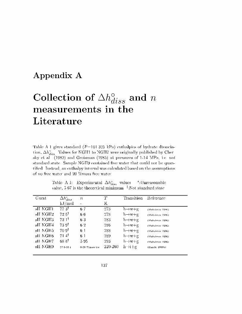
Appendix A
Collection of �h�diss and n
measurements in the
Literature
Table A.1 gives standard (P=101.325 kPa) enthalpies of hydrate dissocia-tion, �h�diss. Values for NGH1 to NGH7 were originally published by Cher-sky et al. (1982) and Groisman (1985) at pressures of 1-14 MPa, i.e. notstandard state. Sample NGH9 contained free water that could not be quan-ti�ed. Instead, an enthalpy interval was calculated based on the assumptionsof no free water and 20 %mass free water.
Table A.1: Experimental �h�diss values. �:Unreasonablevalue, 5.67 is the theoretical minimum. y:Not standard state.
Guest �h�diss n T Transition ReferencekJ/mol - K
sII NGH1 77.3y 6.7 273 h!w+g (Maksimov 1996)
sII NGH2 72.5y 6.6 278 h!w+g (Maksimov 1996)
sII NGH3 72.1y 6.3 283 h!w+g (Maksimov 1996)
sII NGH4 73.9y 6.2 286 h!w+g (Maksimov 1996)
sII NGH5 70.9y 6.1 288 h!w+g (Maksimov 1996)
sII NGH6 71.4y 6.1 289 h!w+g (Maksimov 1996)
sII NGH7 68.8y 5.95 293 h!w+g (Maksimov 1996)
sII NGH9 27.8-33.1 0-20 %mass ice 220-260 h!i+g (Handa 1988b)
137

138APPENDIX A. ENTHALPY AND HYDRATE NUMBERMEASUREMENTS
Table A.1: Experimental �h�diss values. �:Unreasonablevalue, 5.67 is the theoretical minimum. y:Not standard state.
Guest �h�diss n T Transition ReferencekJ/mol - K
sI NGH8 17.50 CH4 � 5:91H2O 273 h!i+g (Handa 1988b)
CH4 54:19 � 0:28 6:00 � 0:01 273.15 h!w+g (Handa 1986c)
CH4 54.36 7.00 273.15 h!w+g (Roberts et al. 1941)
CH4 67.85 6.3 273.15 h!w+g (de Roo et al. 1983)
CH4 55.12 273.15 h!w+g (Deaton and Frost 1946)
CH4 55.07 273.15 h!w+g (McLeod and Campbell 1961)
CH4 53.41 273.15 h!w+g (Marshall et al. 1964)
CH4 18:13 � 0:27 6:00 � 0:01 160-210 h!i+g (Handa 1986c)
CH4 19.06 7.18 273.15 h!i+g (Frost and Deaton 1946)
CH4 23.37 7.4 273.15 h!i+g (de Roo et al. 1983)
C2H6 71:80 � 0:38 7:67 � 0:02 273.15 h!w+g (Handa 1986c)
C2H6 69.71 7 273.15 h!w+g (Roberts et al. 1941)
C2H6 73.88 273.15 h!w+g (Deaton and Frost 1946)
C2H6 86.32 273.15 h!w+g (Reamer et al. 1952)
C2H6 76.09 273.15 h!w+g (Holder and Grigoriou 1980)
C2H6 25:70 � 0:37 7:67 � 0:02 190-250 h!i+g (Handa 1986c)
C2H6 23.75 273.15 h!i+g (Frost and Deaton 1946)
C3H8 129:2 � 0:4 17:0 � 0:1 273.15 h!w+g (Handa 1986c)
C3H8 109.1 273.15 h!w+g (Reamer et al. 1952)
C3H8 126.9 273.15 h!w+g (Frost and Deaton 1946)
C3H8 27:00 � 0:33 17:0 � 0:1 210-260 h!i+g (Handa 1986c)
C3H8 27.91 17.95 275.15 h!i+g (Frost and Deaton 1946)
C3H8 28.30 273.15 h!i+g (Holder and Kamath 1982)
C3H8 26.68 273.15 h!i+g (Holder and Godbole 1982)
i-C4H10 133.2 17 assumed 273.15 h!w+g (Handa 1988a)
i-C4H10 132 273.15 h!w+g (Uchida and Hayano 1964)
i-C4H10 122.4 273.15 h!w+g (Rouher and Barduhn 1969)
i-C4H10 131 273.15 h!w+g (Schneider and Farrar 1968)
i-C4H10 31:07 � 0:20 17 assumed 273.15 h!i+g (Handa 1988a)
i-C4H10 31.31 273.15 h!i+g (Holder and Godbole 1982)

APPENDIX A. ENTHALPY AND HYDRATE NUMBERMEASUREMENTS139
Table A.1: Experimental �h�diss values. �:Unreasonablevalue, 5.67 is the theoretical minimum. y:Not standard state.
Guest �h�diss n T Transition ReferencekJ/mol - K
(CH3)3CH 133:2 � 0:3 17 273.15 h!w+g (Handa 1986c)
(CH3)3CH 132 273.15 h!w+g (Uchida and Hayano 1964)
(CH3)3CH 122.4 274.2 h!w+g (Rouher and Barduhn 1969)
(CH3)3CH 131 273.15 h!w+g (Schneider and Farrar 1968)
(CH3)3CH 31:07 � 0:20 230-260 h!i+g (Handa 1986c)
(CH3)3CH 31.31 256.5 h!i+g (Holder and Godbole 1982)
CO2 57:98 � 7% 281 h!w+g (Nagayev et al. 1979)
Kr 56.3 5.0� 273.15 h!w+g (de Forcrand 1923)
Kr 58.2 273.15 h!w+g (Stackelberg 1949)
Kr 56:20 � 0:25 6.10 273.15 h!w+g (Handa 1986a)
Kr 19:54 � 0:24 6.10 273.15 h!i+g (Handa 1986a)
Kr 20.5 6.0 273.15 h!i+g (Barrer and Edge 1967)
Xn 63:23 � 0:19 6.29 273.15 h!w+g (Handa 1988a)
Xn 61:96 � 0:19 5.90 273.15 h!w+g (Handa 1986a)
Xn 69.2 6.6 273.15 h!w+g (de Forcrand 1925)
Xn 69.9 273.15 h!w+g (Stackelberg 1949)
Xn 61:67 � 0:84 6.0 273.15 h!w+g (Aaldijk 1971)
Xn 64.0 6.0 273.15 h!w+g (Ewing and Ionescu 1974)
Xn 26:50 � 0:17 5.90 273.15 h!i+g (Handa 1986a)
Xn 25:43 � 0:17 6:29 � 0:03 273.15 h!i+g (Handa 1986b)
Xn 24.0 6.0 211-268 h!i+g (Barrer and Edge 1967)
Xn 25:79 � 0:41 6.0 263-273 h!i+g (Aaldijk 1971)
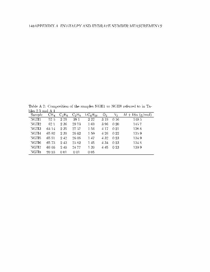
140APPENDIX A. ENTHALPY AND HYDRATE NUMBERMEASUREMENTS
Table A.2: Composition of the samples NGH1 to NGH8 referred to in Ta-bles 2.3 and A.1.Sample CH4 C2H6 C3H8 i-C4H10 O2 N2 M + 18n (g/mol)
NGH1 52.5 2.79 39.1 2.22 3.19 0.16 149.5NGH2 62.1 2.36 29.73 1.69 3.96 0.20 145.7NGH3 64.14 2.35 27.57 1.56 4.17 0.21 138.8NGH4 65.02 2.39 26.62 1.50 4.26 0.22 135.9NGH5 65.51 2.42 26.08 1.47 4.32 0.23 134.9NGH6 65.73 2.43 25.82 1.45 4.34 0.23 134.8NGH7 66.66 2.49 24.77 1.39 4.45 0.23 130.9NGH8 99.93 0.01 0.01 0.05

Appendix B
Experiments and Findings
Leading to the Preliminary
Calorimetric Method
B.1 Alternative Schemes for a Calorimetric Method
Heat has to be supplied to dissociate hydrate . The total heat is in part dueto dissociation of the hydrate itself, but also due to melting of the free waterpresent as ice. In the introductory experiments (Section 6.3.1) the sampleswere heated at ambient pressure. This yielded a single peak at about 273 K.This peak represented both ice melting and hydrate dissociation. The mainchallenge in calorimetric analysis of NGH was to develop a method thatenables the separation of these two heat contributions.
It was clear that the sample had to be pressurized by a gas. The hydrateforming natural gas was the �rst choice. Trial and error was important asthe work proceeded. Three principal schemes were pursued. For the nexttwo paragraphs, note that the speci�ed temperatures and scanning rateswere only the initial assumptions.
Schemes 1 and 3. The sample was heated under pressure. This yieldedone peak around 273 K (ice melting) and one peak at a higher tem-perature (hydrate dissociation). In Scheme 1 the scanning rate wasincreased from 0.01 K/min to 4 K/min after the ice peak. In Scheme 3the scanning rate was constant at 0.05 K/min.
141

142 APPENDIX B. DEVELOPING THE PRELIMINARY METHOD
Scheme 2. The sample was �rst heated under pressure to produce an icemelting peak at 273 K. Then the sample was refrigerated again andthe pressure relieved. During the second heating sequence at ambientpressure one peak due do combined ice melting and hydrate dissocia-tion was seen at 273 K. The scanning rate was 0.05 K in both heatingsequences.
B.2 Individual Tests
Two issues were addressed: First, it was required that the thermal responsedue to ice melting and hydrate dissociation were well separated. Second,it was necessary to gain a quantitative understanding of how to interpretthe heat signals detected for each process (melting and dissociation). Anumber of tests were carried out to �nd ways to meet these two requirements.Selected tests are presented in detail in the following. They are treatedin the same order as they were carried out, thus the progress of systemunderstanding is also communicated.
B.2.1 Tests with Natural Gas
Test 1, Scheme 3 modi�ed, Figure B.1
This was a modi�cation of Scheme 3 where an isothermal sequence was usedbetween the peaks. Natural gas was used to pressurize the sample 2.1 MPa.The gas composition was the same as during hydrate formation; ethane(5 %mol) and propane (3 %mol) in methane. The idea was that by usingthe hydrate forming gas to establish pressure, this would impose the leastdisturbances on the hydrate system. The isotherm between the two peaksallowed complete ice melting before further heating and subsequent hydratedissociation.
Peak separation was good, but the drawback was that the baseline shiftedwhen going from scanning mode to isothermal mode. This complicatedthe peak integration. Since accurate integration is essential, this way ofseparating the peaks was abandoned. When the data were processed, anunreasonable low hydrate number was found, n=1.33, while the ideal (the-oretical minimum) hydrate number is 5.67. Base line shift may explain thisin part, but there is more to it, as will be demonstrated.

B.2. INDIVIDUAL TESTS 143
Test 2, Scheme 3, Figure B.2
In this test the same NG mixture as in Test 1 was used to pressurize thesample (3.0 MPa), but now the isotherm in the scanning cycle was omitted.The sample was heated from 253 K to almost 313 K at a heating rate of0.05 K/min. The low start temperature was to make sure the base line hadstabilized before the �rst peak (ice). The high stop temperature was tomake sure that the last peak (hydrate) should come to a completion.
Peak separation was not good, but when the data were analyzed, a reason-able hydrate number was found; n=6.05. The ideal hydrate number is 5.67.The speci�c enthalpy of hydrate dissociation was �hdiss=534.2 J/g. Thisway of treating the sample yielded promising results, but little con�dencewas put in the results since the peak separation was not good. The exother-mic response between the peaks could be explained by hydrate formation.It was concluded that the procedure in this test was unreliable.
Test 3, Scheme 3, Figure B.3
The pressure was 8.0 MPa. This was not a feasible procedure as the ther-mogram was full of undesirable peaks with considerable exothermic andendothermic integrals. One reason for the complicated peak pattern is prob-ably due to desorption of natural gas from the water that formed as the icemelted. Desorption is explained since the ice froze at around 9 MPa whichis about 1 MPa higher than the pressure used in this test. Hydrate probablyformed too.
B.2.2 Tests with Nitrogen
Test 4, Scheme 3, Figure B.4
Pressurizing with natural gas was not successful. It was decided to trypressurize with nitrogen. Nitrogen too is a hydrate former, but not at thepressure-temperature conditions applied during these tests. The peak sep-aration was not good. In this test the heating rate was 0.05 K/min. Lowerrates yielded even poorer separation. Tests with higher heating rates werenot tried.
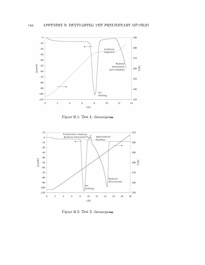
144 APPENDIX B. DEVELOPING THE PRELIMINARY METHOD
-110
-100
-90
-80
-70
-60
-50
-40
-30
-20
-10
0
0 2 4 6 8 10 12 14
t [h]
Q [m
W]
230
240
250
260
270
280
290
T [K
]
Icemelting
Hydratedissociation
(not complete)
Isothermsequence
Figure B.1: Test 1, thermogram.
-110
-100
-90
-80
-70
-60
-50
-40
-30
-20
-10
0
10
0 2 4 6 8 10 12 14 16 18 20
t [h]
Q [m
W]
250
260
270
280
290
300
310
T [K
]
Icemelting
Hydratedissociation
Approximatebaseline
Exothermic responce(hydrate formation?)
Figure B.2: Test 2, thermogram.

B.2. INDIVIDUAL TESTS 145
-140
-120
-100
-80
-60
-40
-20
0
20
40
0 2 4 6 8 10 12 14 16 18 20
t [h]
Q [m
W]
250
260
270
280
290
300
310
T [K
]
Icemelting
Hydratedissociation
Approximate baseline Pattern notunderstood
Figure B.3: Test 3, thermogram.
-70
-60
-50
-40
-30
-20
-10
0
10
0 2 4 6 8 10 12 14
t [h]
Q [m
W]
255
260
265
270
275
280
285
290
295
T [K
]Approximate baseline
Icemelting
Hydratedissociation
Figure B.4: Test 4, thermogram.
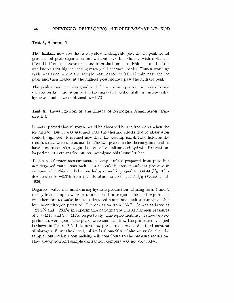
146 APPENDIX B. DEVELOPING THE PRELIMINARY METHOD
Test 5, Scheme 1
The thinking now was that a very slow heating rate past the ice peak wouldgive a good peak separation but without base line shift as with isotherms(Test 1). From the above tests and from the literature (H�ohne et al. 1996) itwas known that higher heating rates yield narrower peaks. Thus a scanningcycle was tried where the sample was heated at 0.01 K/min past the icepeak and then heated at the highest possible rate past the hydrate peak.
The peak separation was good and there are no apparent sources of errorsuch as peaks in addition to the two expected peaks. Still an unreasonablehydrate number was obtained, n=1.73.
Test 6: Investigation of the E�ect of Nitrogen Absorption, Fig-
ure B.5
It was expected that nitrogen would be absorbed by the free water when theice melted. But it was assumed that the thermal e�ects due to absorptioncould be ignored. It seemed now that this assumption did not hold, as theresults so far were unreasonable. The two peaks in the thermograms had tohave a more complex origin than only ice melting and hydrate dissociation.Experiments were carried out to investigate this issue further.
To get a reference measurement, a sample of ice prepared from pure butnot degassed water, was melted in the calorimeter at ambient pressure inan open cell. This yielded an enthalpy of melting equal to 334.44 J/g. Thisdeviated only �0:2% from the literature value of 333.7 J/g (Weast et al.1986).
Degassed water was used during hydrate production. During tests 4 and 5the hydrate samples were pressurized with nitrogen. The next experimentwas therefore to make ice from degassed water and melt a sample of thisice under nitrogen pressure. The deviation from 333.7 J/g was as large as�23:2% and �23:0% in experiments performed at initial nitrogen pressuresof 5.05 MPa and 5.00 MPa, respectively. The reproducibility of these two ex-periments were good. The peaks were smooth. How the pressure developedis shown in Figure B.5. It is seen how pressure decreased due to absorptionof nitrogen. Since the density of ice is about 90% of the water density, thesample contraction upon melting will contribute to the pressure reduction.How absorption and sample contraction compare was not calculated.

B.2. INDIVIDUAL TESTS 147
5
5.05
5.1
5.15
5.2
5.25
5.3
1 2 3 4 5 6 7 8 9t [h]
P [M
Pa]
Pressure increase according to PV=znRT
Pressure decrease due to nitrogenbeing absorbed by water at 273 K
Figure B.5: Test 6. Up to 273 K the pressure increased according toPV = znRT . At 273 K there was a sudden drop as nitrogen was absorbedby the water. Upon further heating the pressure continues to increase.
The following had been shown. When a sample of ice prepared from degassedwater is melted under a nitrogen atmosphere of 5.0 MPa, the speci�c heatof melting is 256:5 � 0:5 J/g. This has important consequences for hydratenumber calculations - so far, a melting enthalpy of 333.5 J/g had beenused in calculations, under the assumption that thermal e�ects of nitrogenabsorption were negligible. This assumption failed. A di�erent value had tobe used.
This also had consequences as far as the procedure it self is concerned. Itwas assumed that nitrogen would also absorb in the water that was formedwhen the hydrate dissociated under nitrogen pressure. Further complica-tions regarding data analysis follows. This tends to favor Scheme 2, whereonly ice is melted under pressure, while hydrate is dissociated at ambientpressure.

148 APPENDIX B. DEVELOPING THE PRELIMINARY METHOD
Test 7, Scheme 2, Figure B.6
During the �rst cycle the sample was pressurized. The peak was due toice melting. The peak was neat, so the integration did not pose any prob-lems. The sample was then refrozen and the pressure was taken down toambient and the calorimeter cells left open to the surrounding air. In thesecond cycle there also was one single peak (Figure B.6). It was due tocombined ice melting and hydrate dissociation. Test 7 was repeated, andworked �ne as far as operation and peak separation are concerned. The des-orption of gas from the melted ice has to be accounted for when integratingthe ice melting peak. This illustrates the need for some "fundamental" data:
� Enthalpy of melting when ice from degassed water is melted at elevatedpressure.
� Enthalpy of melting when ice formed at elevated pressure pressure ismelted at ambient pressure.
-110
-90
-70
-50
-30
-10
2 3 4 5 6 7 8 9 10 11 12
t [h]
Q [m
W]
260
265
270
275
280
285
290
T [K
]
Hydrate dissociationandice melting
Figure B.6: Test 7, Hydrate dissociation cycle.

B.2. INDIVIDUAL TESTS 149
B.2.3 Tests with Methane
Test 8, Scheme 2 extended
Tests 1 to 7 showed that natural gas and nitrogen caused complications dueto absorption and desorption, and probably hydrate formation in the caseof natural gas. The idea now was to pressurize the sample with methane.But still the melting of the ice (free water) will be accompanied by absorp-tion/desorption. The corresponding thermal e�ect contributed to the melt-ing peak. This contribution could not be quanti�ed. Thus, it was proposedto extend Scheme 2 by applying a sample conditioning step.
Sample conditioning refers to melting the ice that formed under an elevatednatural gas pressure, to allow the water phase with the dissolved natural gasto equilibrate with methane. Thus, the part of the sample that actually wasconditioned or pretreated, was the ice. After the conditioning, the samplewas refrozen.
In a second cycle, the sample was heated once again to melt the ice. Nowthe ice melted under a gas with which it was equilibrated as it froze. Ac-cordingly, the thermal e�ect of absorption/desorption was negligible andthe peak was due to melting only. To calculate the amount of free water itwas necessary to know the speci�c enthalpy of ice melting when freezing andmelting took place at the same pressure. This value was determined in sepa-rate experiments to be 342.63 J/g for a methane pressure of 1.7 MPa. It wasassumed that the uncertainty is�0:5%, as in earlier ice melting experiments.
The pressure 1.7 MPa was chosen as follows. The sample needed to be pres-surized above the hydrate curve for the NG used to produce the hydrates. Atthe same time, the pressure had to be below the hydrate curve for methane.This should make the system non-reactive - it was assumed that hydratewill neither form nor dissociate. The pressure was needed to melt the icewithout dissociating the hydrate. This governed the temperature interval ofinterest. The water could not be heated above 276 K. The lowest temper-ature is about 263 K. If the hydrate curves are consulted (Figure 6.5) it isseen that an initial pressure of 1.7 MPa was appropriate.
E�ects due to ethane and propane in the free water are assumed negligible forthe following reasons. The ice contains ethane corresponding to an ethanepartial pressure of about 0:05Pproduction. The origin of 0.05 is that the NGused to produce the hydrate contains 5 %mol ethane. A similar argument
150 APPENDIX B. DEVELOPING THE PRELIMINARY METHOD
can be set forth for propane, which was present at 3 %mol in the NG. Nearlyall of the ethane and propane in the water that formed during the sampleconditioning will desorb in order to attain phase equilibria. Only negligibleamounts of sII hydrate may form during the following cooling sequence, ifat all. Further, the system was operated in a pressure-temperature regionwhere methane hydrate do not form. In short, the driving forces for absorp-tion/desorption and hydrate formation/dissociation are negligible after theconditioning step.
What remained was to dissociate the hydrate to �nd the speci�c enthalpy ofdissociation. This could be done either at some elevated pressure (1.7 MPa)by just continuing the heating of the sample. Alternatively, the sample couldbe refrozen while still pressurized and the system depressurized to ambientpressure before dissociation. The latter alternative was chosen since it is theleast involving, and sources of error are reduced. Note that when NGH isdissociated in the NGH chain, this will also take place at ambient pressure.It is known from the introductory experiments (Section 6.3.1) that in thiscase, hydrate dissociation will be accompanied by ice melting and that thepeak will show at about 273 K. The heat contribution from ice melting anddesorption of absorbed gases, notably methane, can be calculated. Speci�centhalpy of dissociation is then found from the mass and energy balance.What is needed is the enthalpy of melting at ambient pressure of ice thatformed under 1.7 MPa methane. This value was determined experimentallyin a separate test as 344.38 J/g.
The results of Test 8 were reasonable (n = 4:7 � 1:8, f = 59 � 1%), butthe random error in n was large. This could be reduced by using a moreaccurate balance when measuring the sample mass and by increasing thesample mass. Both means would reduce the random errors.
Test 9 and 10, Scheme 2 extended
These tests were carried out according to the same procedures as in Test 7,but with a more accurate balance; �0:002 g in stead of �0:01 g. The sam-ple mass was increased from about 0.92 g to 1.100 g (Test 9) and 1.001 g(Test 10). Because of the higher sample masses the ice melting peaks be-came wider and the criterion of not heating the sample above the hydrateequilibrium line, was violated. It was concluded that a sample mass of about0.95 g was the highest feasible.

B.2. INDIVIDUAL TESTS 151
Test 11, Scheme 2 extended
This test was carried out just as Test 8 except now the pressure was 1.7 MPa(it was 1.5 MPa in Test 8). The sample had been stored at 224 K for7 weeks and at 257 K for 2 days. The hydrate number was low, but ifthe same uncertainty interval as in Test 8 was assumed, then the errorinterval covered the ideal hydrate number. The speci�c enthalpy of hydratedissociation was 315.8 J/g. The amount of free water was 70 %mass. Thethermograms looked as in Figures 6.2 to 6.4 which were collected during thesame type of test.

152 APPENDIX B. DEVELOPING THE PRELIMINARY METHOD

Appendix C
Thermal and Compositional
Properties - Estimates
The models and correlations reported in the literature (Chapter 2) are nowused to estimate thermophysical and compositional properties of sII naturalgas hydrate. The numbers are mostly estimated independently of each otherand may not be fully consistent. The results are collected in Table 6.2.
Composition
The hydrated gas is assumed to consist of methane (89 %mol), ethane(6 %mol) and propane (5 %mol). This is about the same hydrate com-position as obtained during run 1 in the fractionation experiments wherethe P = 7:5 MPa and T = 275 K, giving a driving force of �T = 16 K. Theaverage molar mass of the hydrated gas is then 18.24 g/mol.
The hydrate number is assumed to be n=6. This is a reasonable assumptionas the ideal hydrate number is 5.67, and since a considerable driving force(�T = 16 K) is a relevant assumption.
Enthalpy of Dissociation
�h�diss is estimated in Figure C.1 using the Clausius-Clapeyron equationaround P = 1:01 MPa. Phase equilibriumdata are simulated using CSMHYD(Sloan 1998) and assuming a natural gas of ethane (5 %mol) and propane(3 %mol) in methane.
153

154 APPENDIX C. PROPERTIES - ESTIMATES
T > 273.15 KlnP = -8765.8/T + 31.905Slope = -8765.8
T < 273.15 KlnP = -2787.2/T + 10.014Slope = -2787.2
-0.3
-0.25
-0.2
-0.15
-0.1
-0.05
0
0.05
0.1
0.15
0.00362 0.00363 0.00364 0.00365 0.00366 0.00367 0.00368 0.00369 0.0037
1/T [1/K]
lnP
[-]
Figure C.1: Clausius-Clapeyron plot around 101,325 Pa. The phase equi-librium data are for a gas of ethane (5 %mol) and propane (3 %mol) inmethane and were obtained using CSMHYD.
Assuming z � 1 gives for T = 274:8 K and P = 1:01 MPa:�h�diss = �zaR � �1(�8785)8:413 J/mol = 73.0 kJ/mol.Multiplying by 1000=(MNG + 18n), using n = 6 and M = 18:24 g/mol(assumptions made above), this converts into 578 J/g. This is a relevantestimate for sII natural gas hydrate.
Using the equilibrium values MNG � 27 g/mol and n � 7:4 obtained byCSMHYD, 73 kJ/mol converts into 456 J/g. This shows that the formationconditions, notably the driving force, has a big impact on �hdiss (J/g) viathe average molar mass of the hydrated gas, MNG. For T < 273:15 K, theslope is �2787:2 K. Then, �hdiss = �zaR � �1(�2787:2)8:314 J/mol =23 kJ/mol. The way �hdiss suddenly changes at T = 273:15 K is re ectedin the change of slope in the Clausius-Clapeyron plot.

APPENDIX C. PROPERTIES - ESTIMATES 155
The �hdiss (kJ/mol) values obtained above compare to experimental val-ues in the literature. Maksimov (1996) reported 68.8-77.3 kJ/mol for sIINGH above 273.15 K. It has been shown here, how a Clausius-Clapeyronsimulation yielded an intermediate value; 73.0 kJ/mol. Handa (1988b) re-ported 27.8-33.1 kJ/mol for sII NGH below 273.15 K. The deviation be-tween the lower value (27.8 kJ/mol) and the Clausius-Clapeyron predic-tion (23 kJ/mol) is about 20%. Using the guest size dependent model(Section 2.4.2) by Sloan and Fleyfel (1992) the value �hdiss = 79 kJ/mol(T > 273 K) is found.
The correlation by Selim and Sloan (1990) in Section 2.4.4 yields �hdiss=446:12 � 103 � 132:638 � 274:8 = 410 J/g. This value di�ers �29% from578 J/g obtained above, and �10% from the value 456 J/g, also obtainedabove but assuming equilibrium values of MNG and n. The deviations maybe explained since this correlation applies to hydrate in sediment. Thecorrelation is not ment to apply to bulk hydrate. The correlation is basedon Clausius-Clapeyron calculations and using equilibrium data, which isprobably why it compares better to 456 J/K. Also note that the correlationis given for natural gas hydrate, without specifying the composition of thehydrate or the hydrate forming gas.
An intresting thing can be seen if the �hdiss values in Table 2.3 are cor-rected for the hydrate number variations. Let the value n = 6.7 for sampleNGH1 be the reference, since it applied in the case where the pressure waslowest (1.1 MPa) and closest to standard pressure. Table C.1 is referredto. For NGH7, �hdiss becomes 6:7
5:95 � 68:8 kJ/mol = 77:4 kJ/mol, whichis close to the value 77.3 kJ/mol for sample NGH1. The largest deviationfrom the reference value (77.3 kJ/mol) is 4.8% (NGH2) and with an aver-age deviation of 1.9%. The corresponding numbers for the original data are11.0% and 7.4%, respectively. This shows how the variations in the hydratenumber largly account for the variations in �hdiss (kJ/mol). This re ectsthat breaking the hydrogen bonds in the lattice accounts for a large portionof �hdiss. Another intresting manipulation of the �hdiss data in Table 2.3is to multiply by 1000=(MNG + 18n) to convert from kJ/mol to J/g. Thelargest deviation from the reference value (517 J/g) is 5.2% (NGH4) andwith an average deviation of 2.5%.
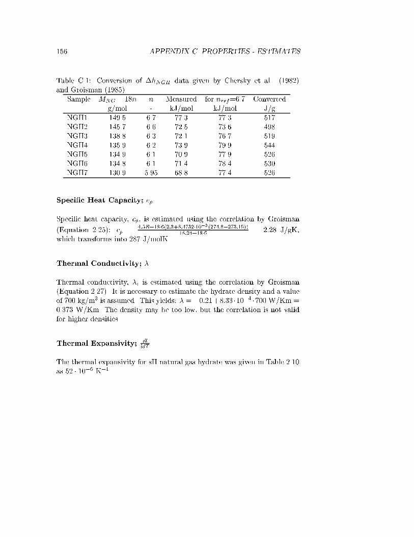
156 APPENDIX C. PROPERTIES - ESTIMATES
Table C.1: Conversion of �hNGH data given by Chersky et al. (1982)and Groisman (1985).
Sample MNG + 18n n Measured for nref=6.7 Convertedg/mol - kJ/mol kJ/mol J/g
NGH1 149.5 6.7 77.3 77.3 517NGH2 145.7 6.6 72.5 73.6 498NGH3 138.8 6.3 72.1 76.7 519NGH4 135.9 6.2 73.9 79.9 544NGH5 134.9 6.1 70.9 77.9 526NGH6 134.8 6.1 71.4 78.4 530NGH7 130.9 5.95 68.8 77.4 526
Speci�c Heat Capacity; cp
Speci�c heat capacity, cp, is estimated using the correlation by Groisman
(Equation 2.25): cp = 4:5R+18�6(2:3+8:4732�10�3(274:8�273:15))18:24+18�6 = 2:28 J/gK,
which transforms into 287 J/molK.
Thermal Conductivity; �
Thermal conductivity, �, is estimated using the correlation by Groisman(Equation 2.27). It is necessary to estimate the hydrate density and a valueof 700 kg/m3 is assumed. This yields: � = �0:21+8:33 �10�4 �700 W/Km =0.373 W/Km. The density may be too low, but the correlation is not validfor higher densities.
Thermal Expansivity; dlldT
The thermal expansivity for sII natural gas hydrate was given in Table 2.10as 52 � 10�6 K�1.

Appendix D
Determination of
Fractionation Model
Parameters
Average Reactor Gas Composition for Zero Driving Force
To develop the fractionation model it was necessary to estimate the averagereactor gas composition in case of �T = 0. This is done in Figures D.1and D.2 for methane and propane, respectively.
k-value Determination
The fractionation model includes a system dependent constant k. k-valueswere determined for methane and propane in least squares plots with
�(model(k;�T )�data(�T ))2
on the ordinate and k on the abscissa for each pressure. The model expressesthe content of ethane in the hydrate as C2;diss = 100� (CC1;diss +CC3;diss)to make the mass balance close at 100 %mol. Concequently, the k-valuesfor ethane are not needed. The plots follow in Figures D.3 to D.10.
Extrapolation of k(P; i) to 9.0 MPa
The model was extrapolated to P = 9:0 MPa. k-value estimates for methaneand propane were found graphically in Figure D.11.
157

158 APPENDIX D. PARAMETER DETERMINATION
92
92.2
92.4
92.6
92.8
93
93.2
93.4
93.6
93.8
94
0 2 4 6 8 10 12 14 16 18
∆T [K]
CC
1,re
ac [%
mol
]
7.5 MPa
6.0 MPa
4.5 MPa
3.0 MPa
3.0 MPa
4.5 MPa
6.0 & 7.5 MPa
93.775
92.950
92.825
Figure D.1: Extrapolation of CC1;reac = (CC1;feed + CC1;reac)=2 to �T =0. CC1;reac is the gas phase concentration of methane at the end of anexperiment.
1.8
2
2.2
2.4
2.6
2.8
3
3.2
0 2 4 6 8 10 12 14 16 18∆T [K]
CC
3,re
ac [%
mol
]
7.5 MPa
6.0 MPa
4.5 MPa
3.0 MPa
30 bara
45 bara
60 & 75 bara
2.575
2.400
1.800
Figure D.2: Extrapolation of CC3;reac = (CC3;feed + CC3;reac)=2 to �T =0. CC3;reac is the gas phase concentration of propane at the end of anexperiment.
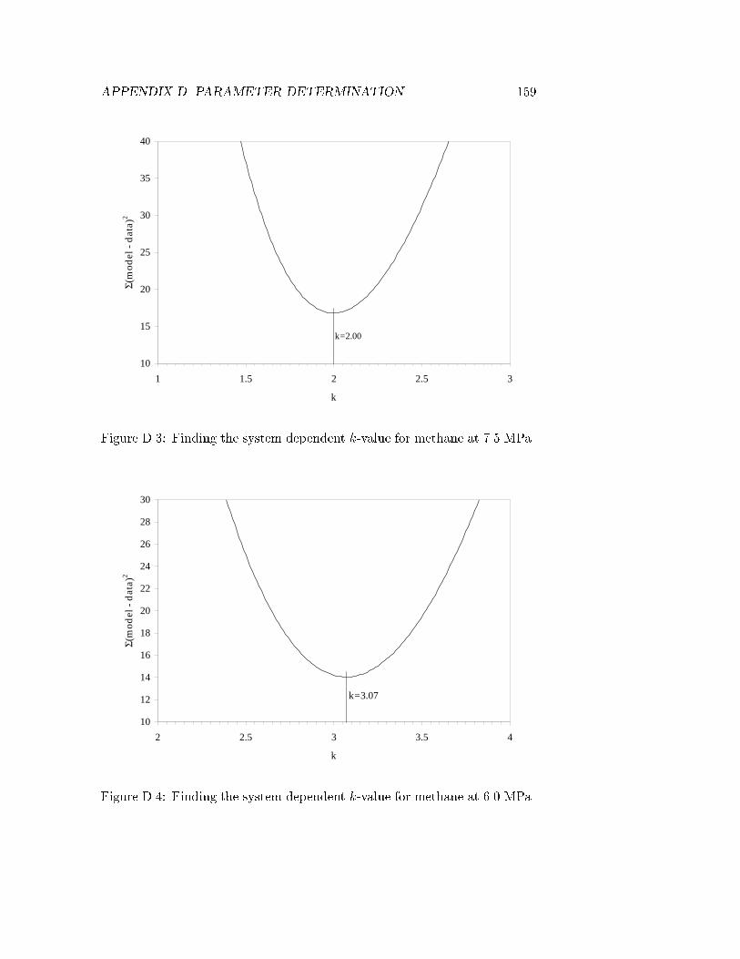
APPENDIX D. PARAMETER DETERMINATION 159
10
15
20
25
30
35
40
1 1.5 2 2.5 3
k
Σ(m
odel
- d
ata)
2
k=2.00
Figure D.3: Finding the system dependent k-value for methane at 7.5 MPa.
10
12
14
16
18
20
22
24
26
28
30
2 2.5 3 3.5 4
k
Σ(m
odel
- d
ata)
2
k=3.07
Figure D.4: Finding the system dependent k-value for methane at 6.0 MPa.

160 APPENDIX D. PARAMETER DETERMINATION
20
22
24
26
28
30
32
34
36
38
40
2 2.5 3 3.5 4
k
Σ (m
odel
-dat
a)2
k=3.18
Figure D.5: Finding the system dependent k-value for methane at 4.5 MPa.
15
16
17
18
19
20
21
22
23
24
25
3 3.5 4 4.5 5
k
Σ (m
odel
-dat
a)2
k=3.99
Figure D.6: Finding the system dependent k-value for methane at 3.0 MPa.

APPENDIX D. PARAMETER DETERMINATION 161
0
5
10
15
20
25
30
35
40
45
50
0 0.5 1 1.5 2
k
Σ (m
odel
-dat
a)2
k=1.11
Figure D.7: Finding the system dependent k-value for propane at 7.5 MPa.
0
2
4
6
8
10
12
14
16
18
20
1 1.5 2 2.5 3
k
Σ (m
odel
-dat
a)2
k=1.69
Figure D.8: Finding the system dependent k-value for propane at 6.0 MPa.

162 APPENDIX D. PARAMETER DETERMINATION
0
2
4
6
8
10
12
14
16
18
20
1 1.5 2 2.5 3
k
Σ(m
odel
-dat
a)2
k=1.82
Figure D.9: Finding the system dependent k-value for propane at 4.5 MPa.
0
5
10
15
20
25
30
1 1.5 2 2.5 3
k
Σ(m
odel
-dat
a)2
k=1.93
Figure D.10: Finding the system dependent k-value for propane at 3.0 MPa.

APPENDIX D. PARAMETER DETERMINATION 163
Propane:k(P) = -0.1727P + 2.544
Methane:k(P) = -0.4053P + 5.188
0
0.5
1
1.5
2
2.5
3
3.5
4
4.5
2 3 4 5 6 7 8 9P [MPa]
k [-
]
Methane
Propane
Propane intercept: k~1.0
Methane intercept: k~1.5
Figure D.11: Linear regression (extrapolation) of experimental k-values at3.0, 4.5, 6.0 and 7.5 MPa to estimate k-values at 9.0 MPa.

Appendix E
List of Publications
The following publications were made as part of the present work:
Gudmundsson, J.S., Andersson, V., Levik, O.I. and Parlaktuna, M.: Nat-ural Gas Hydrates: A new Gas-Transportation Form, J. Petrol. Technol.51(4):66-67, 1999.
Gudmundsson, J.S., Andersson, V., Durgut, I., Levik, O.I. and Mork, M.:NGH on FPSO - Slurry Process and Cost Estimate, SPE Annual TechnicalConference and Exhibition, Houston, 3-6 October 1999. SPE paper 56629.
Levik, O.I. and Gudmundsson, J.S.: Calorimetry to Study Metastabilityof Natural Gas Hydrate at Atmospheric Pressure and Temperatures below0 �C, 3rd. Intl. Conf. on Gas Hydrates, Salt Lake City, 18-22 July, 1999.
Gudmundsson, J.S., Andersson, V., Levik, O.I. and Mork, M.: HydrateTechnology for Capturing Stranded Gas, 3rd. Intl. Conf. on Gas Hydrates,Salt Lake City, 18-22 July, 1999.
Gudmundsson, J.S., Parlaktuna, M., Levik, O.I. and Andersson, V.: Labo-ratory for Continuous Production of Natural Gas Hydrates, 3rd. Intl. Conf.on Gas Hydrates, Salt Lake City, 18-22 July, 1999.
Gudmundsson, J.S., Andersson, V., Levik, O.I. and Parlaktuna, M.: Hy-drate Concept for Capturing Associated Gas, SPE European Petroleumconference, The Hague, 20-22 October, 1998, SPE paper 50598.
Gudmundsson, J.S., Andersson, V. and Levik, O.I.: Gas Storage and Trans-port Using Hydrate, Proc. O�shore Mediterranean Conference, Ravenna,19-21 March, 2:1075-1083, 1997.
164