thermoelectric cooling: designing novel home appliances · peltier modules thermal behavior is...
TRANSCRIPT
Thermoelectric Cooling: designing novel home appliances
Paulo Ricardo Braga Moniz Quental
Thesis to obtain the Master of Science Degree in
Mechanical Engineering
Supervisor: Prof. Manuel Frederico Tojal de Valsassina Heitor
Examination Committee
Chairperson: Prof. Mário Manuel Gonçalves da Costa Supervisor: Prof. Manuel Frederico Tojal de Valsassina Heitor
Member of the Committee: Dr. Hugo Filipe Diniz Policarpo
November 2015


iii
Acknowledgements
I am grateful to Professor Manuel Heitor, for the support and encouragement and all the opportunities
that he ever presented to me.
To my family, especially to my mother and my father, who gave me the opportunity to achieve what they
never had the possibility to.
My colleagues José Pinto Ferreira and Ruben Moutinho and Mellow Inc., their knowledge and support
added a lot to this work.
To Rita Rosa, Daniel Fonseca, João Eirinha, Guilherme Farinha, Hugo Policarpo, Bruno Mendonça and
Pipa, for your effort in the correction and revision of this thesis, for all the company and support and the
most important of all, for their friendship.
Cannot forget all the people that were my companions on this path in Técnico - in Projecto FST, Fórum
Mecânica, Conselho Pedagógico and other adventures.

iv
Resumo
Dispositivos de arrefecimento térmoelétrico são cada vez mais uma opção para aplicações laboratoriais
e domésticas. O respectivo campo de aplicações é crescente, fomentado por pelos baixos preços da
tecnologia e o desenvolvimento de pequenos electrodomésticos. Estes sistemas consistem na
montagem de módulo de Peltier e dissipadores de calor, que no contexto deste trabalho são arrefecido
a ar. Assim, o objectivo consiste em desenvolver um dispositivo de arrefecimento termoeléctrico
compacto, para um robô de cozinha – sous vide machine – com um enquadramento em
desenvolvimento de produto. O robô de cozinha já se encontra no processo de desenho para fabrico,
sendo desde já o volume geométrico disponível e as condições de experiência de utilização de produto,
contrangimentos.
Neste trabalho, começa-se por apresentar uma breve revisão das tecnologias de refrigeração
existentes, com aplicações semelhantes à pretendida, assim como uma breve avaliação do mercado.
Prosegue-se com a formulação do problema, o respectivo projecto mecânico, e o modelo matemático
predictivo do processo de arrefecimento. De seguida estima-se o comportamento térmico dos módulos
de Peltier e caractteriza-se a montagem do sistema é caracterizada e as configurações possíveis
detalhadas.Segue-se à análise numérica aos dissipadores de calor, usando o ANSYS Icepak,
considerando que estão submetidos a diferentes condições e modelos de turbulência nomeadamente,
os modelos de turbulência Spalar-Allmaras, ERNG e ERTE. Para terminar, uma geometria de
dissipador adequada para a aplicação e apresentam-se as principais conclusões e recomendações
para trabalhos futuros.
Destas, é de salientar que os dissipadores de calor de fluxo horizontal e vertical avaliados, mostram
desempenhos semelhantes. Para efeitos de redução de ruído e melhor eficiência energética, os
modelos de fluxo horizontal são a melhor opção. Os dissipadores obtidos por extrusão apresentam
desempenhos semelhantes aos de alhetas coladas, apesar da maior dimensão. Os custos estimados
justificam um estudo futuro de arrefecimento líquido.
Palavras-chave: Peltier, dissipador de calor, termoeléctrico, Icepak, design, arrefecimento
v
Abstract
Thermoelectric cooling technologies have proven themselves as reliable alternatives for laboratorial
applications and small home appliances. Its range of applications is growing, fomented by lower prices
of technology and development of small house products as cooking machines and small refrigerator.
They consist of an assembly of Peltier modules and heat sinks, which in the scope of this work, are air
cooled.
The objective of this thesis is to develop a compact thermoelectric cooling assembly for a kitchen
countertop home appliance – a sous vide cooking machine – falling under the scope of new product
development. The appliance design process, must take in consideration the volume available and user
experience related constraints.
In this work, a brief review of existent technologies and market assessment, precedes the problem
formulation, mechanical design and mathematical prediction model of the refrigeration process. The
Peltier modules thermal behavior is estimated and the thermoelectric assembly is characterized. The
heat sinks chosen are then described. Numerical simulation of the heat sinks, submitted to different
conditions and turbulence models, simulated on ANSYS ICEPAK, are presented. The Spalart-Allmaras,
the ERNG Model and the ERTE Model are the turbulence models considered. To conclude, a heat sink
geometry, especially design for the appliance is suggested, and the main conclusions and some
recommendations for future works are presented.
From these, it is noted that the vertical and horizontal flow heatsinks assessed are predicted to have
similar performance. For noise reduction and better efficiency, the horizontal flow is the best
configuration. Extruded heat sink can achieve similar performance to bonded fins heat sinks, but with a
significant mass increase. The estimated costs justify the study of liquid cooling solutions.
Keywords: Peltier, heat sink, thermoelectric, Icepak, design, cooling
vi
Contents
Acknowledgements ................................................................................................................................. iii
Resumo ................................................................................................................................................... iv
Abstract.....................................................................................................................................................v
Contents .................................................................................................................................................. vi
List of figures ......................................................................................................................................... viii
List of tables .............................................................................................................................................x
1. Introduction .......................................................................................................................................... 1
1.2 Sous vide / Slow cooking ............................................................................................................... 2
1.3 Smart sous vide machine .............................................................................................................. 3
1.4 Methodologies ................................................................................................................................ 4
1.5 Technologies review ...................................................................................................................... 5
1.6 Thermoelectric applications – home appliances market review ................................................ 7
1.7. Thermoelectric cooling assemblies – market review ................................................................ 9
2. Problem Statement ............................................................................................................................ 13
3 Towards a New Product ..................................................................................................................... 16
3.1 Incorporation in the product ......................................................................................................... 17
3.2 Hardware selection ...................................................................................................................... 19
3.2.1 Peltier Modules...................................................................................................................... 19
3.2.2 Heat Sinks ............................................................................................................................. 21
3.2.3 Materials selection .................................................................................................................... 24
3.3 Mathematical Modeling of the cooling system ............................................................................. 25
3.5 Test implementation ..................................................................................................................... 26
3.5.1 Material needed to test procedure ........................................................................................ 27
4 Numerical Analysis ............................................................................................................................. 28
4.1 Governing Equations of Fluid Flow .............................................................................................. 28
4.2 Simulation setup and preliminary results ..................................................................................... 30
4.3 Detailed calculations .................................................................................................................... 33
4.4 Heat sink development ................................................................................................................ 33
5 Product Development ......................................................................................................................... 35
5.1 Peltier behavior approximation – conclusions ............................................................................. 35

vii
5.2 Results of mathematical model and configuration conclusions ................................................... 36
5.2.1 Model EX00001H .................................................................................................................. 36
6 Final remarks ...................................................................................................................................... 38
6.1 Next steps .................................................................................................................................... 39
References ............................................................................................................................................ 40
Annexes ................................................................................................................................................. 42
A1 Cost estimation ............................................................................................................................. 44
B1 Ruben Moutinho’s Interview summary ......................................................................................... 46
B2 José Pinto Ferreira’s Interview summary ..................................................................................... 46
C1 MATLAB routine ........................................................................................................................... 47
viii
List of figures
Figure 1 – The central activity of design [1]............................................................................................. 1
Figure 2 – a) water circulator sous vide machine; b) heated container sous vide machine. .................. 2
Figure 3 – Cooked pork tenderloin, a) pan cooking b) sous vide cooking. ............................................. 3
Figure 4 – Mellow prototype and smartphone application and features presentation. ........................... 3
Figure 5 – Product life cycle tree [1]. ....................................................................................................... 4
Figure 6 – Methodology scheme for cooling module development. ........................................................ 5
Figure 7 – Example of non-cyclic refrigeration in which sardines are kept on ice [4]. ............................ 6
Figure 8 – Refrigeration cycles schematics: a) reverse-Rankine vapor-compression; b) Brighton gas
cycle. ........................................................................................................................................................ 6
Figure 9 – Photograph of refrigerator unit with a “small” refrigerator compressor [5]. ............................ 6
Figure 10 – Thermoelectric refrigeration: a) TEC based cooling module schematic; b) Peltier Module [6].
................................................................................................................................................................. 7
Figure 11 – 12V Cooler – cooling module image [5]. .............................................................................. 7
Figure 12 – Peltier module mount detail and heat sink thermal paste in the heat exchanger side [5].... 8
Figure 13 – Beer tender heat sink [5]. ..................................................................................................... 8
Figure 14 – Mini bar front and rear with heat sink [5]. ............................................................................. 8
Figure 15 – Small dehumidifier [5]. .......................................................................................................... 9
Figure 16 – Laird AA-034-12-22-00-00 [8]. ............................................................................................. 9
Figure 17 – Laird DA-075-24-02-00-00 [8]. ............................................................................................. 9
Figure 18 – TETech CP-061 Thermoelectric cooling module of “Horizontal flow” [9]. .......................... 10
Figure 19 – CP-061 Performance chart [9]. .......................................................................................... 10
Figure 20 – TETech CP-110: a) model; b) performance chart [10]. ...................................................... 11
Figure 21 – Laird DA-075-24-02 performance chart [11]. ..................................................................... 11
Figure 22 – Laird DA-039-12-02 performance chart. ............................................................................ 12
Figure 23 – Kryotherm TCA380-24-AS: a) CAD model; b) performance chart [10]. ............................. 12
Figure 24 – Double wall lid. ................................................................................................................... 13
Figure 25 – Double walled lid thermal resistance. ................................................................................ 14
Figure 25 – Thermoelectric cooling assembly cut view. ........................................................................ 15
Figure 27 – Thermoelectric cooling assembly goals. ............................................................................ 16
Figure 28 – Thermoelectric cooling assembly components. ................................................................. 17
Figure 29 – CAD model illustration of the appliance volume available. ................................................ 17
Figure 30 – CAD model illustration vertical flow with 1 outlet. .............................................................. 18
Figure 31 – Horizontal flow assembly section view of a thermoelectric cooling assembly. .................. 18
Figure 32 – Vertical flow assembly section view of a thermoelectric cooling assembly. ...................... 18
Figure 33 – TEC1-12715 Power consumption chart [21]. ..................................................................... 19
Figure 34 – TEC1-12715 Cooling rate chart [21]. ................................................................................. 20
Figure 35 – Heat sink submitted to 150W, room temperature of 25 ºC [5]. ......................................... 22
Figure 36 – AAVID 78440 thermal resistance for forced convection [25]. ............................................ 22
ix
Figure 37 – CES EduPack 2013 metals relation between price and thermal conductivity – the area
bounded by red is the one in use. ......................................................................................................... 24
Figure 38 – CES EduPack 2013 selected area, plus condition that material must be processed by
extrusion. ............................................................................................................................................... 24
Figure 39 – Thermocouples location in the thermoelectric assembly for experience. .......................... 27
Figure 40 – Experimental setup for data aquisition of the experiment. ................................................. 27
Figure 41 – Geometric preview of AA74925 SA125. ........................................................................... 31
Figure 42 – Fan working curve and Heat sink (WV17080H) caused pressure drop [Pa], related with the
air flow [m3/s] [5]. ................................................................................................................................... 32
Figure 43 – EX00001H – proposed model geometry. ........................................................................... 34
Figure 44 – TETech working curves and modeled curve. ..................................................................... 35
Figure 45 – Purposed geometry possible setups results. ..................................................................... 36
x
List of tables
Table 1 – Lid walls conduction thermal resistance parameters ............................................................ 14
Table 2 – Lid walls convection thermal resistance parameters............................................................. 14
Table 3 – Peltier modules technical information.................................................................................... 21
Table 4 – Heat sinks data from Wakefield-Vette and AAVID. ............................................................... 23
Table 5 – Heat sinks thermal resistance at 30 liters per second flow rate. ........................................... 32
Table 6 – Numerical simulation final results. Flow rate of 0.03m3/s. ..................................................... 33
Table 7 – EX00001H numerical simulation final results. Flow rate of 0.03m3/s. ................................... 34
Table 8 – Purposed thermoelectric assembly selection results. .......................................................... 37
Table A.1 9– ANSYS Icepak results ...................................................................................................... 42
Table A.2 9– Heat sink estimated weight and cost, for one and two Peltier modules assembly. ... Error!
Bookmark not defined.
Table A.3 9– Ensemble costs [USD] ..................................................................................................... 45
1
1. Introduction
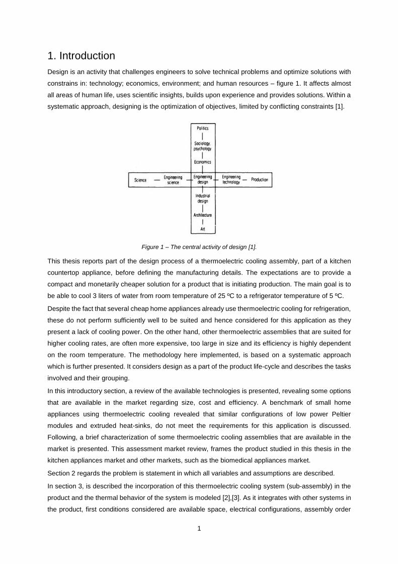
Design is an activity that challenges engineers to solve technical problems and optimize solutions with
constrains in: technology; economics, environment; and human resources – figure 1. It affects almost
all areas of human life, uses scientific insights, builds upon experience and provides solutions. Within a
systematic approach, designing is the optimization of objectives, limited by conflicting constraints [1].
Figure 1 – The central activity of design [1].
This thesis reports part of the design process of a thermoelectric cooling assembly, part of a kitchen
countertop appliance, before defining the manufacturing details. The expectations are to provide a
compact and monetarily cheaper solution for a product that is initiating production. The main goal is to
be able to cool 3 liters of water from room temperature of 25 ºC to a refrigerator temperature of 5 ºC.
Despite the fact that several cheap home appliances already use thermoelectric cooling for refrigeration,
these do not perform sufficiently well to be suited and hence considered for this application as they
present a lack of cooling power. On the other hand, other thermoelectric assemblies that are suited for
higher cooling rates, are often more expensive, too large in size and its efficiency is highly dependent
on the room temperature. The methodology here implemented, is based on a systematic approach
which is further presented. It considers design as a part of the product life-cycle and describes the tasks
involved and their grouping.
In this introductory section, a review of the available technologies is presented, revealing some options
that are available in the market regarding size, cost and efficiency. A benchmark of small home
appliances using thermoelectric cooling revealed that similar configurations of low power Peltier
modules and extruded heat-sinks, do not meet the requirements for this application is discussed.
Following, a brief characterization of some thermoelectric cooling assemblies that are available in the
market is presented. This assessment market review, frames the product studied in this thesis in the
kitchen appliances market and other markets, such as the biomedical appliances market.
Section 2 regards the problem is statement in which all variables and assumptions are described.
In section 3, is described the incorporation of this thermoelectric cooling system (sub-assembly) in the
product and the thermal behavior of the system is modeled [2],[3]. As it integrates with other systems in
the product, first conditions considered are available space, electrical configurations, assembly order

2
and functioning goals are clearly set and defined. This is followed by the selection of products and
materials, regarding heat-sinks, Peltier modules, insulating materials and custom parts materials. The
modeling of the thermal system as well as the respective governing equations are presented. This model
allows to estimate the refrigeration in the appliance vat, with a determined set of heat sinks and Peltier
modules. This modeling is supported by CAD and material selection software. In order to compare the
estimated results with experimental data, this section also presents a setup of data acquisition and
describes the materials needed to implement it.
Following, in section 4, the performance of previously selected heat-sink profiles is simulated using
numerical methods [4], [5]. For it, commercial software ANSYS ICEPAK is used, in which the heat-sinks
are analyzed in force convection [6], to obtain the working points of the thermal resistance and the fan
pressure drop. The flow is considered turbulent for all the simulated conditions. Hence, three different
first order advanced turbulence models are applied to each mesh: Spalart and Allmaras [7], Enhanced
RNG and Enhanced Realizable k-e [8]. In this section are also presented some modifications
suggestions of the heat sink profiles that may increase their performance. Based on these modifications,
a geometry of heat-sink is suggested.
In section 5, are presented the main results in which is analyzed: the respective impact and effects in
the product integration as well as; the estimated the cost of the proposed solution.
To conclude, in section 6 are presented the main conclusions of this thesis and some guide lines for
future works are suggested, e.g., a liquid cooled solution.
Next, the sous vide technique is introduced.
1.2 Sous vide / Slow cooking
Sous vide means “under vacuum” and is a slow cooking technique. It may be described as cooking food
in plastic pouches in a low temperature (~60ºC) water bath, for long periods of time. More specifically,
this technique consists in placing food inside a high density propylene food safe bag, or container, which
is immersed in a controlled cooking temperature water bath, in order to achieve the best texture and
flavors. Meat is usually cooked between 55ºC and 70ºC for periods of time that vary between 1 and 72
hours. The heating water bath may be obtained using a circulator, as illustrated by figure 2 a), or a
heated container as the one illustrated by figure 2 b).
a)
b)
Figure 2 – a) water circulator sous vide machine; b) heated container sous vide machine.
3
http://www.sciencedirect.com/science/article/pii/S1878450X11000035#bib24
The sous vide technique ensures not only sterilization, but also an even cooking result, where a similar
piece of meat cooked in a pan, as illustrated by figure 3 a), and in sous vide, as illustrated by figure 3 b),
respectively, may be visually compared. With sous vide, the meat is evenly cooked with a safe
temperature in the core as well as in the outside without overcooking the meat.
Figure 3 – Cooked pork tenderloin, a) pan cooking b) sous vide cooking.
Sous vide cooking is often considered as a modernist and difficult technique that only top restaurant
and molecular cuisine chefs employ.
1.3 Smart sous vide machine
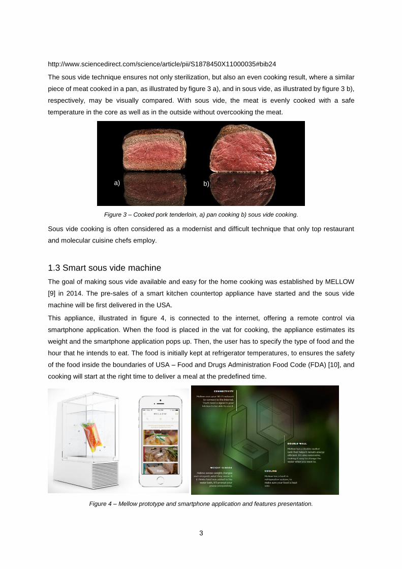
The goal of making sous vide available and easy for the home cooking was established by MELLOW
[9] in 2014. The pre-sales of a smart kitchen countertop appliance have started and the sous vide
machine will be first delivered in the USA.
This appliance, illustrated in figure 4, is connected to the internet, offering a remote control via
smartphone application. When the food is placed in the vat for cooking, the appliance estimates its
weight and the smartphone application pops up. Then, the user has to specify the type of food and the
hour that he intends to eat. The food is initially kept at refrigerator temperatures, to ensures the safety
of the food inside the boundaries of USA – Food and Drugs Administration Food Code (FDA) [10], and
cooking will start at the right time to deliver a meal at the predefined time.
Figure 4 – Mellow prototype and smartphone application and features presentation.
a) b)
4
The development of a cooling assembly that can fit this appliance and match performance to ensure
food safety at the design for manufacturing phase of MELLOW, is the driving motivation of this work.
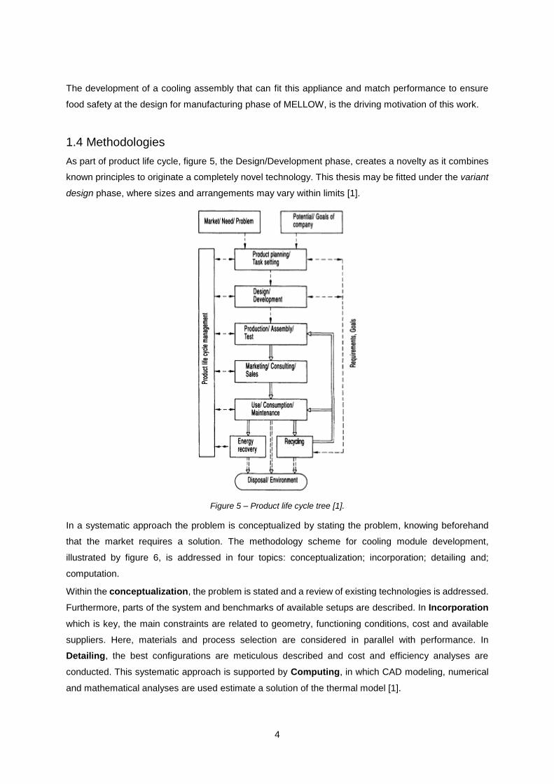
1.4 Methodologies
As part of product life cycle, figure 5, the Design/Development phase, creates a novelty as it combines
known principles to originate a completely novel technology. This thesis may be fitted under the variant
design phase, where sizes and arrangements may vary within limits [1].
Figure 5 – Product life cycle tree [1].
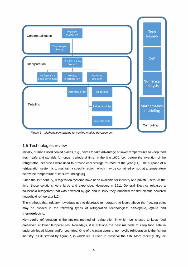
In a systematic approach the problem is conceptualized by stating the problem, knowing beforehand
that the market requires a solution. The methodology scheme for cooling module development,
illustrated by figure 6, is addressed in four topics: conceptualization; incorporation; detailing and;
computation.
Within the conceptualization, the problem is stated and a review of existing technologies is addressed.
Furthermore, parts of the system and benchmarks of available setups are described. In Incorporation
which is key, the main constraints are related to geometry, functioning conditions, cost and available
suppliers. Here, materials and process selection are considered in parallel with performance. In
Detailing, the best configurations are meticulous described and cost and efficiency analyses are
conducted. This systematic approach is supported by Computing, in which CAD modeling, numerical
and mathematical analyses are used estimate a solution of the thermal model [1].
5
1.5 Technologies review
Initially, humans used cooled places, e.g., caves to take advantage of lower temperatures to keep food
fresh, safe and storable for longer periods of time. In the late 1600, i.e., before the invention of the
refrigerator, icehouses were used to provide cool storage for most of the year [11]. The purpose of a
refrigeration system is to maintain a specific region, which may be contained or not, at a temperature
below the temperature of its surroundings [6].
Since the 19th century, refrigeration systems have been available for industry and private users. At the
time, those solutions were large and expensive. However, in 1911 General Electrics released a
household refrigerator that was powered by gas and in 1927 they launched the first electric powered
household refrigerator [12].
The methods that industry nowadays use to decrease temperature to levels above the freezing point
may be divided in the following types of refrigeration technologies: non-cyclic, cyclic and
thermoelectric.
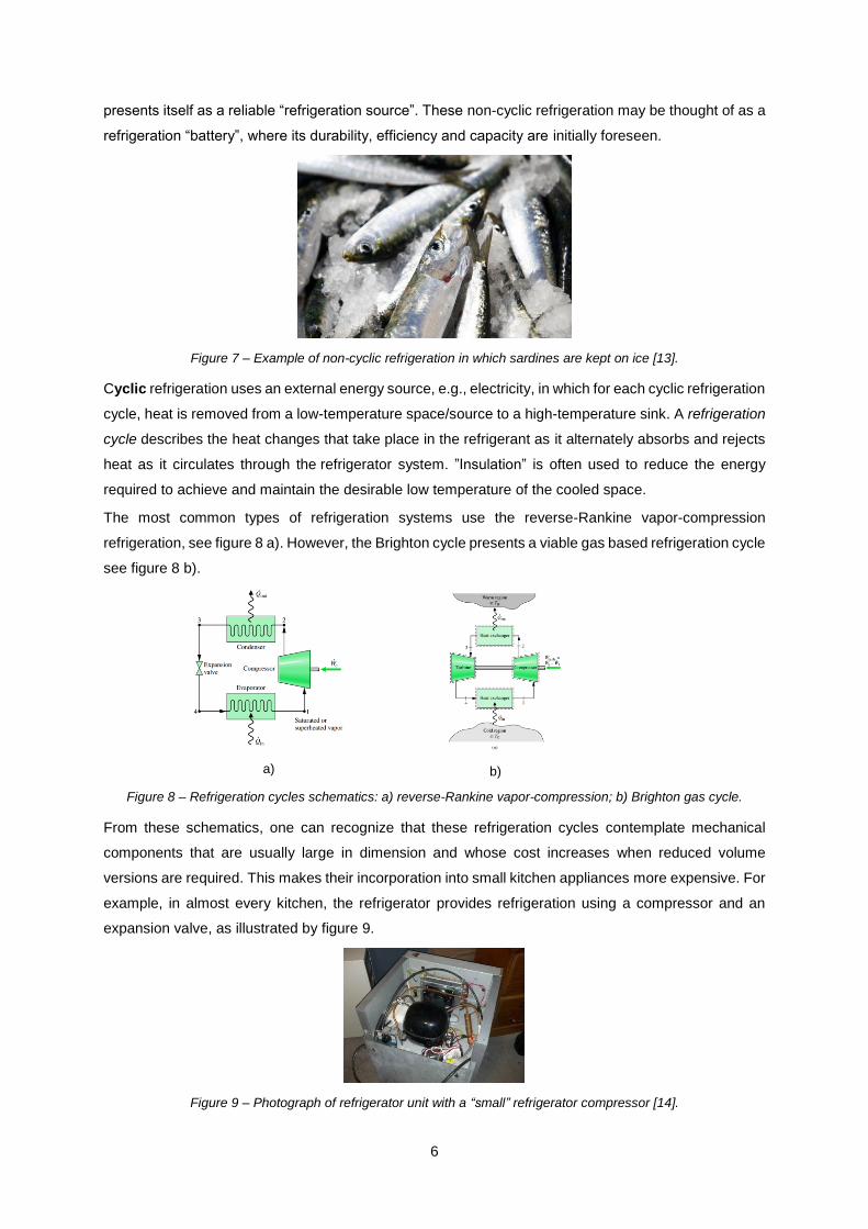
Non-cyclic refrigeration is the ancient method of refrigeration in which ice is used to keep food
preserved at lower temperatures. Nowadays, it is still one the best methods to keep food safe in
underprivileged labors and/or countries. One of the main users of non-cyclic refrigeration is the fishing
industry, as illustrated by figure 7, in which ice is used to preserve the fish. More recently, dry ice
Problem Statement
Towards a new Product
Performance goals deffinition
Product incorporation
Assembly order
Materials Selection
Heat sinks
Peltier modules
miscelaneous
Tecnhologies Review
Conceptualization
Incorporation
Detailing
Computing
Tech Review
CAD
Numerical analysis
Mathematical modeling
Figure 6 – Methodology scheme for cooling module development.
6
presents itself as a reliable “refrigeration source”. These non-cyclic refrigeration may be thought of as a
refrigeration “battery”, where its durability, efficiency and capacity are initially foreseen.
Figure 7 – Example of non-cyclic refrigeration in which sardines are kept on ice [13].
Cyclic refrigeration uses an external energy source, e.g., electricity, in which for each cyclic refrigeration
cycle, heat is removed from a low-temperature space/source to a high-temperature sink. A refrigeration
cycle describes the heat changes that take place in the refrigerant as it alternately absorbs and rejects
heat as it circulates through the refrigerator system. ”Insulation” is often used to reduce the energy
required to achieve and maintain the desirable low temperature of the cooled space.
The most common types of refrigeration systems use the reverse-Rankine vapor-compression
refrigeration, see figure 8 a). However, the Brighton cycle presents a viable gas based refrigeration cycle
see figure 8 b).
a)
b)
Figure 8 – Refrigeration cycles schematics: a) reverse-Rankine vapor-compression; b) Brighton gas cycle.
From these schematics, one can recognize that these refrigeration cycles contemplate mechanical
components that are usually large in dimension and whose cost increases when reduced volume
versions are required. This makes their incorporation into small kitchen appliances more expensive. For
example, in almost every kitchen, the refrigerator provides refrigeration using a compressor and an
expansion valve, as illustrated by figure 9.
Figure 9 – Photograph of refrigerator unit with a “small” refrigerator compressor [14].
7
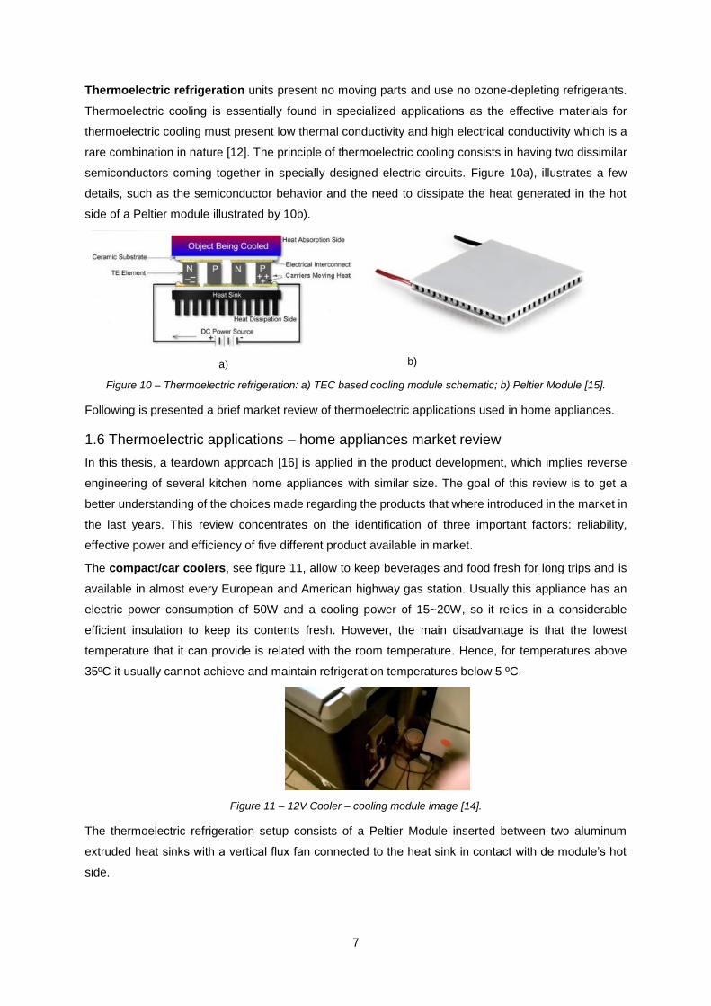
Thermoelectric refrigeration units present no moving parts and use no ozone-depleting refrigerants.
Thermoelectric cooling is essentially found in specialized applications as the effective materials for
thermoelectric cooling must present low thermal conductivity and high electrical conductivity which is a
rare combination in nature [12]. The principle of thermoelectric cooling consists in having two dissimilar
semiconductors coming together in specially designed electric circuits. Figure 10a), illustrates a few
details, such as the semiconductor behavior and the need to dissipate the heat generated in the hot
side of a Peltier module illustrated by 10b).
a)
b)
Figure 10 – Thermoelectric refrigeration: a) TEC based cooling module schematic; b) Peltier Module [15].
Following is presented a brief market review of thermoelectric applications used in home appliances.
1.6 Thermoelectric applications – home appliances market review
In this thesis, a teardown approach [16] is applied in the product development, which implies reverse
engineering of several kitchen home appliances with similar size. The goal of this review is to get a
better understanding of the choices made regarding the products that where introduced in the market in
the last years. This review concentrates on the identification of three important factors: reliability,
effective power and efficiency of five different product available in market.
The compact/car coolers, see figure 11, allow to keep beverages and food fresh for long trips and is
available in almost every European and American highway gas station. Usually this appliance has an
electric power consumption of 50W and a cooling power of 15~20W, so it relies in a considerable
efficient insulation to keep its contents fresh. However, the main disadvantage is that the lowest
temperature that it can provide is related with the room temperature. Hence, for temperatures above
35ºC it usually cannot achieve and maintain refrigeration temperatures below 5 ºC.
Figure 11 – 12V Cooler – cooling module image [14].
The thermoelectric refrigeration setup consists of a Peltier Module inserted between two aluminum
extruded heat sinks with a vertical flux fan connected to the heat sink in contact with de module’s hot
side.
8
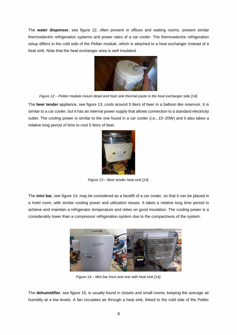
The water dispenser, see figure 12, often present in offices and waiting rooms, present similar
thermoelectric refrigeration systems and power rates of a car cooler. The thermoelectric refrigeration
setup differs in the cold side of the Peltier module, which is attached to a heat exchanger instead of a
heat sink. Note that the heat exchanger area is well insulated.
Figure 12 – Peltier module mount detail and heat sink thermal paste in the heat exchanger side [14].
The beer tender appliance, see figure 13, cools around 5 liters of beer in a balloon like reservoir. It is
similar to a car cooler, but it has an internal power supply that allows connection to a standard electricity
outlet. The cooling power is similar to the one found in a car cooler (i.e., 15~20W) and it also takes a
relative long period of time to cool 5 liters of beer.
Figure 13 – Beer tender heat sink [14].
The mini bar, see figure 14, may be considered as a facelift of a car cooler, so that it can be placed in
a hotel room, with similar cooling power and utilization issues. It takes a relative long time period to
achieve and maintain a refrigerator temperature and relies on good insulation. The cooling power is a
considerably lower than a compressor refrigeration system due to the compactness of the system.
Figure 14 – Mini bar front and rear with heat sink [14].
The dehumidifier, see figure 15, is usually found in closets and small rooms, keeping the average air
humidity at a low levels. A fan circulates air through a heat sink, linked to the cold side of the Peltier
9
module, which pushes condensation of water from the air and stores it in a reservoir. For a power
consumption of 22.5 W the maximum cooling power is approximately 10W.
Figure 15 – Small dehumidifier [14].
The applications and appliances reviewed above present themselves as reliable but too low in power to
match the requirements needed in the work scenario of this thesis. Hence, a thermoelectric cooling
assembly market review is follows.
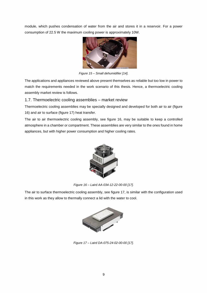
1.7. Thermoelectric cooling assemblies – market review
Thermoelectric cooling assemblies may be specially designed and developed for both air to air (figure
16) and air to surface (figure 17) heat transfer.
The air to air thermoelectric cooling assembly, see figure 16, may be suitable to keep a controlled
atmosphere in a chamber or compartment. These assemblies are very similar to the ones found in home
appliances, but with higher power consumption and higher cooling rates.
Figure 16 – Laird AA-034-12-22-00-00 [17].
The air to surface thermoelectric cooling assembly, see figure 17, is similar with the configuration used
in this work as they allow to thermally connect a lid with the water to cool.
Figure 17 – Laird DA-075-24-02-00-00 [17].
10
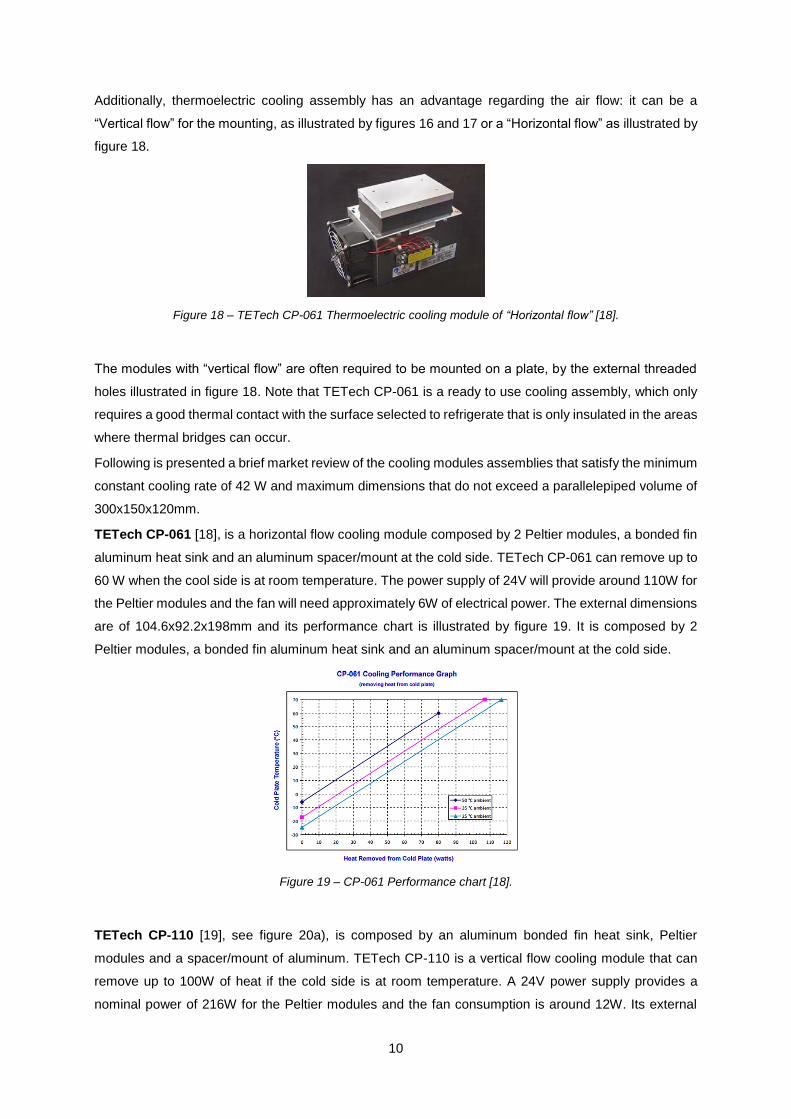
Additionally, thermoelectric cooling assembly has an advantage regarding the air flow: it can be a
“Vertical flow” for the mounting, as illustrated by figures 16 and 17 or a “Horizontal flow” as illustrated by
figure 18.
Figure 18 – TETech CP-061 Thermoelectric cooling module of “Horizontal flow” [18].
The modules with “vertical flow” are often required to be mounted on a plate, by the external threaded
holes illustrated in figure 18. Note that TETech CP-061 is a ready to use cooling assembly, which only
requires a good thermal contact with the surface selected to refrigerate that is only insulated in the areas
where thermal bridges can occur.
Following is presented a brief market review of the cooling modules assemblies that satisfy the minimum
constant cooling rate of 42 W and maximum dimensions that do not exceed a parallelepiped volume of
300x150x120mm.
TETech CP-061 [18], is a horizontal flow cooling module composed by 2 Peltier modules, a bonded fin
aluminum heat sink and an aluminum spacer/mount at the cold side. TETech CP-061 can remove up to
60 W when the cool side is at room temperature. The power supply of 24V will provide around 110W for
the Peltier modules and the fan will need approximately 6W of electrical power. The external dimensions
are of 104.6x92.2x198mm and its performance chart is illustrated by figure 19. It is composed by 2
Peltier modules, a bonded fin aluminum heat sink and an aluminum spacer/mount at the cold side.
Figure 19 – CP-061 Performance chart [18].
TETech CP-110 [19], see figure 20a), is composed by an aluminum bonded fin heat sink, Peltier
modules and a spacer/mount of aluminum. TETech CP-110 is a vertical flow cooling module that can
remove up to 100W of heat if the cold side is at room temperature. A 24V power supply provides a
nominal power of 216W for the Peltier modules and the fan consumption is around 12W. Its external

11
dimensions are 130x140x203mm. However, clearance is required to account for the fan flow. The
performance chart is illustrated by figure 20b) .
a)
b)
Figure 20 – TETech CP-110: a) model; b) performance chart [19].
Laird DA-075-24-02 [20], see figure 17, is an aluminum vertical flow heat sink with a similar TETech
CP-110 configuration. The main difference is that the heat sink is extruded from an aluminum block
instead of using bonded fins. This unit works with a 24V power supply and the nominal power
consumption is 90W, with a maximum cooling power of 71W. The exterior dimensions are of
122x68x230mm. Figure 21 illustrates the performance chart for this model.
Figure 21 – Laird DA-075-24-02 performance chart [20].
Laird DA-039-12-02 [21], is a horizontal flow thermoelectric cooling assembly, with a maximum cooling
power of 40W and a nominal power consumption of 47W. The heat sink is made from extruded aluminum
and the spacer/mount is also aluminum. The exterior dimensions are 65x82x180mm. The performance
chart is illustrated by figure 22.
12
Figure 22 – Laird DA-039-12-02 performance chart.
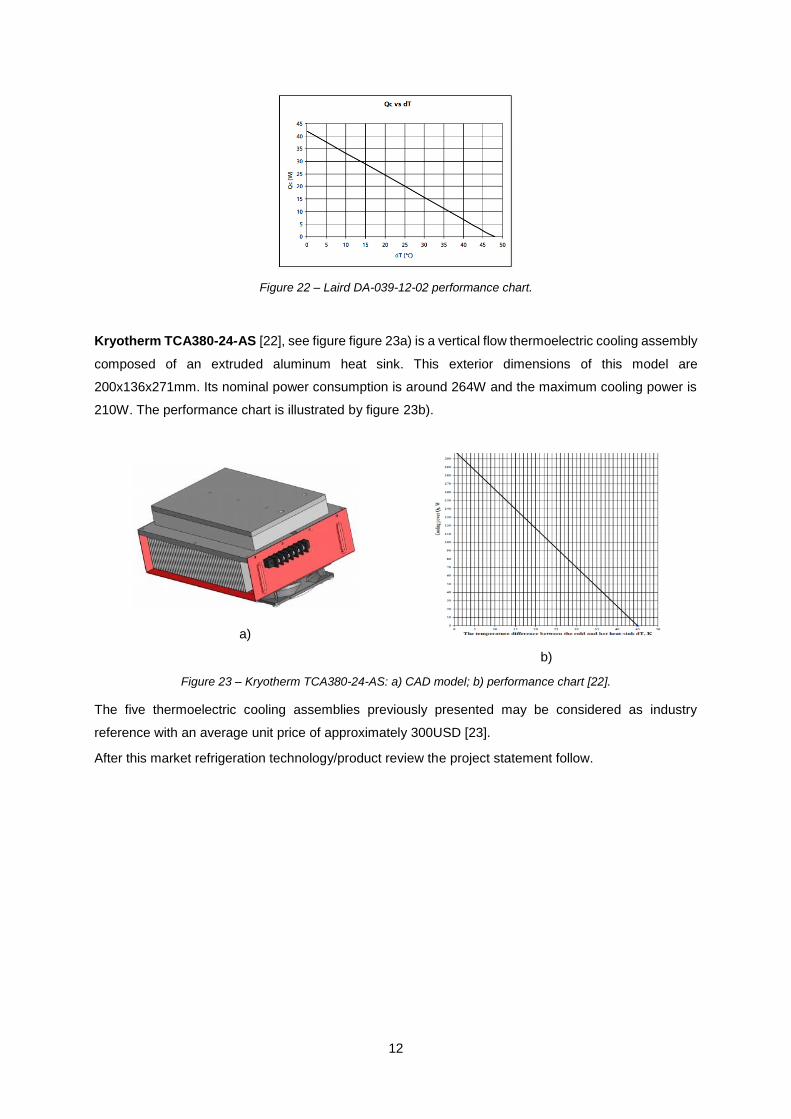
Kryotherm TCA380-24-AS [22], see figure figure 23a) is a vertical flow thermoelectric cooling assembly
composed of an extruded aluminum heat sink. This exterior dimensions of this model are
200x136x271mm. Its nominal power consumption is around 264W and the maximum cooling power is
210W. The performance chart is illustrated by figure 23b).
a)
b)
Figure 23 – Kryotherm TCA380-24-AS: a) CAD model; b) performance chart [22].
The five thermoelectric cooling assemblies previously presented may be considered as industry
reference with an average unit price of approximately 300USD [23].
After this market refrigeration technology/product review the project statement follow.
13
2. Problem Statement
The problem here addressed consists of cooling 3 liters of water, from an initial temperature of 25 ºC to
a final temperature of 5 ºC, in a 2 hour time period. Assuming a constant cooling rate and disregarding
the efficiency losses due to ambient conditions, the total energy, 𝐸𝑇[𝐽], to be remove can be calculated
as
𝐸𝑇 = 𝐶𝑤 ∗ 𝑚𝑤 ∗ ∆𝑇 = 4187 ∗ 3 ∗ (25 − 5) = 251220𝐽, (1)
and the average heat loss rate as
𝑞𝐶̅̅ ̅ =
𝐸𝑇
∆𝑡=
251220
2 ∗ 3600≈ 35𝑊, (2)
where 𝐶𝑤 [𝐽
𝑘𝑔.𝐾] is the water specific heat capacity, 𝑚𝑤[𝑘𝑔] is the mass of water in the lid, ∆𝑇[℃ 𝑜𝑟 𝐾] is
the difference between initial and final temperature of the water.
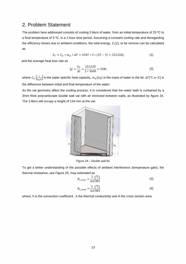
As the vat geometry affect the cooling process, it is considered that the water bath is contained by a
3mm thick polycarbonate double wall vat with air enclosed between walls, as illustrated by figure 24.
The 3 liters will occupy a height of 134 mm at the vat.
Figure 24 – Double wall lid.
To get a better understanding of the possible effects of ambient interference (temperature gain), the
thermal resistance, see Figure 25, may estimated as
where, h is the convection coefficient , k the thermal conductivity and A the cross section area.
𝑅𝑡,𝑐𝑜𝑛𝑣 =
1
ℎ𝐴[℃
W] (3)
𝑅𝑡,𝑐𝑜𝑛𝑑 =
𝐿
𝑘𝐴[℃
W] (4)
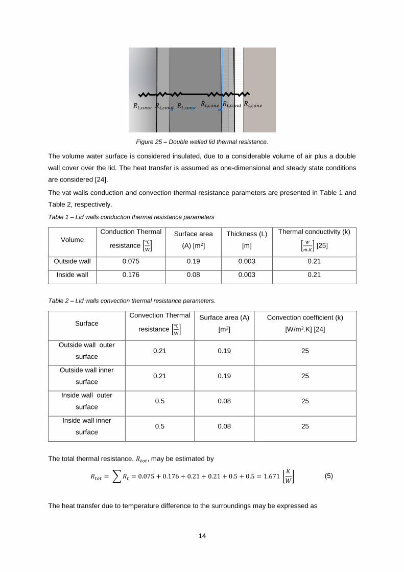
14
Figure 25 – Double walled lid thermal resistance.
The volume water surface is considered insulated, due to a considerable volume of air plus a double
wall cover over the lid. The heat transfer is assumed as one-dimensional and steady state conditions
are considered [24].
The vat walls conduction and convection thermal resistance parameters are presented in Table 1 and
Table 2, respectively.
Table 1 – Lid walls conduction thermal resistance parameters
Volume
Conduction Thermal
resistance [℃
W]
Surface area
(A) [m2]
Thickness (L)
[m]
Thermal conductivity (k)
[𝑊
𝑚.𝐾] [25]
Outside wall 0.075 0.19 0.003 0.21
Inside wall 0.176 0.08 0.003 0.21
Table 2 – Lid walls convection thermal resistance parameters.
Surface
Convection Thermal
resistance [℃
W]
Surface area (A)
[m2]
Convection coefficient (k)
[W/m2.K] [24]
Outside wall outer
surface 0.21 0.19 25
Outside wall inner
surface 0.21 0.19 25
Inside wall outer
surface 0.5 0.08 25
Inside wall inner
surface 0.5 0.08 25
The total thermal resistance, 𝑅𝑡𝑜𝑡, may be estimated by
𝑅𝑡𝑜𝑡 = ∑ 𝑅𝑡 = 0.075 + 0.176 + 0.21 + 0.21 + 0.5 + 0.5 = 1.671 [
𝐾
𝑊] (5)
The heat transfer due to temperature difference to the surroundings may be expressed as
𝑅𝑡,𝑐𝑜𝑛𝑣 𝑅𝑡,𝑐𝑜𝑛𝑑 𝑅𝑡,𝑐𝑜𝑛𝑣 𝑅𝑡,𝑐𝑜𝑛𝑣 𝑅𝑡,𝑐𝑜𝑛𝑑 𝑅𝑡,𝑐𝑜𝑛𝑣
15
𝑞𝑠𝑢𝑟𝑟𝑜𝑢𝑛𝑑𝑖𝑛𝑔𝑠 =
𝑇𝑟𝑜𝑜𝑚 − 𝑇𝑤𝑎𝑡ℎ𝑒𝑟𝑏𝑎𝑡ℎ
𝑅𝑡𝑜𝑡
(6)
This approach is not a verified engineering simulation, it is an approximation based on unidimensional
heat transfer to estimate the order of magnitude of the effect. The materials and specification for the vat
were not yet defined for production.
With this assumption, it is predicted that the cooling of 3 liters of water from 25 ºC to 5 ºC with an average
rate of cooling of 42W (instead of the 35W estimated by Eq. 2) ) will take around 120 minutes. The
specific heat of the water is considered to be 4181 [𝐽
𝑘𝑔.𝐾] [24] and constant during the cooling process.
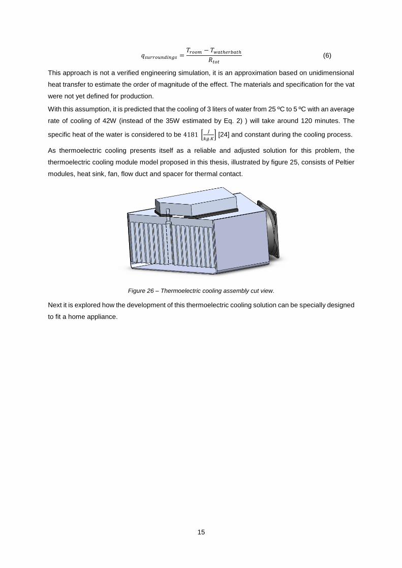
As thermoelectric cooling presents itself as a reliable and adjusted solution for this problem, the
thermoelectric cooling module model proposed in this thesis, illustrated by figure 25, consists of Peltier
modules, heat sink, fan, flow duct and spacer for thermal contact.
Figure 26 – Thermoelectric cooling assembly cut view.
Next it is explored how the development of this thermoelectric cooling solution can be specially designed
to fit a home appliance.
16
3 Towards a New Product
This section explores the development of a cooling solution, particularly designed to fit a home
appliance. A diverse background and experience is of great help as thermoelectric cooling systems are
mainly developed in an industrial setting and there are very few scholar and academic works about this
topic.
The cooling rate is estimated to allow identifying possible assemblies to integrate the home appliance
presented that is segmented by parts and sub-assemblies. Components of the proposed cooling
assemblies are further discussed. The benefits to structural integrity and user experience are also
addressed.
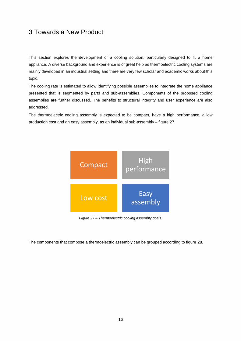
The thermoelectric cooling assembly is expected to be compact, have a high performance, a low
production cost and an easy assembly, as an individual sub-assembly – figure 27.
Figure 27 – Thermoelectric cooling assembly goals.
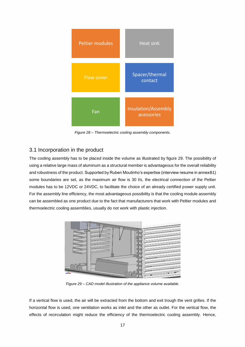
The components that compose a thermoelectric assembly can be grouped according to figure 28.
CompactHigh
performance
Low costEasy
assembly
17
Figure 28 – Thermoelectric cooling assembly components.
3.1 Incorporation in the product
The cooling assembly has to be placed inside the volume as illustrated by figure 29. The possibility of
using a relative large mass of aluminum as a structural member is advantageous for the overall reliability
and robustness of the product. Supported by Ruben Moutinho’s expertise (interview resume in annexB1)
some boundaries are set, as the maximum air flow is 30 l/s, the electrical connection of the Peltier
modules has to be 12VDC or 24VDC, to facilitate the choice of an already certified power supply unit.
For the assembly line efficiency, the most advantageous possibility is that the cooling module assembly
can be assembled as one product due to the fact that manufacturers that work with Peltier modules and
thermoelectric cooling assemblies, usually do not work with plastic injection.
Figure 29 – CAD model illustration of the appliance volume available.
If a vertical flow is used, the air will be extracted from the bottom and exit trough the vent grilles. If the
horizontal flow is used, one ventilation works as inlet and the other as outlet. For the vertical flow, the
effects of recirculation might reduce the efficiency of the thermoelectric cooling assembly. Hence,
Peltier modules Heat sink
Flow coverSpacer/thermal
contact
FanInsulation/Assembly
acessories
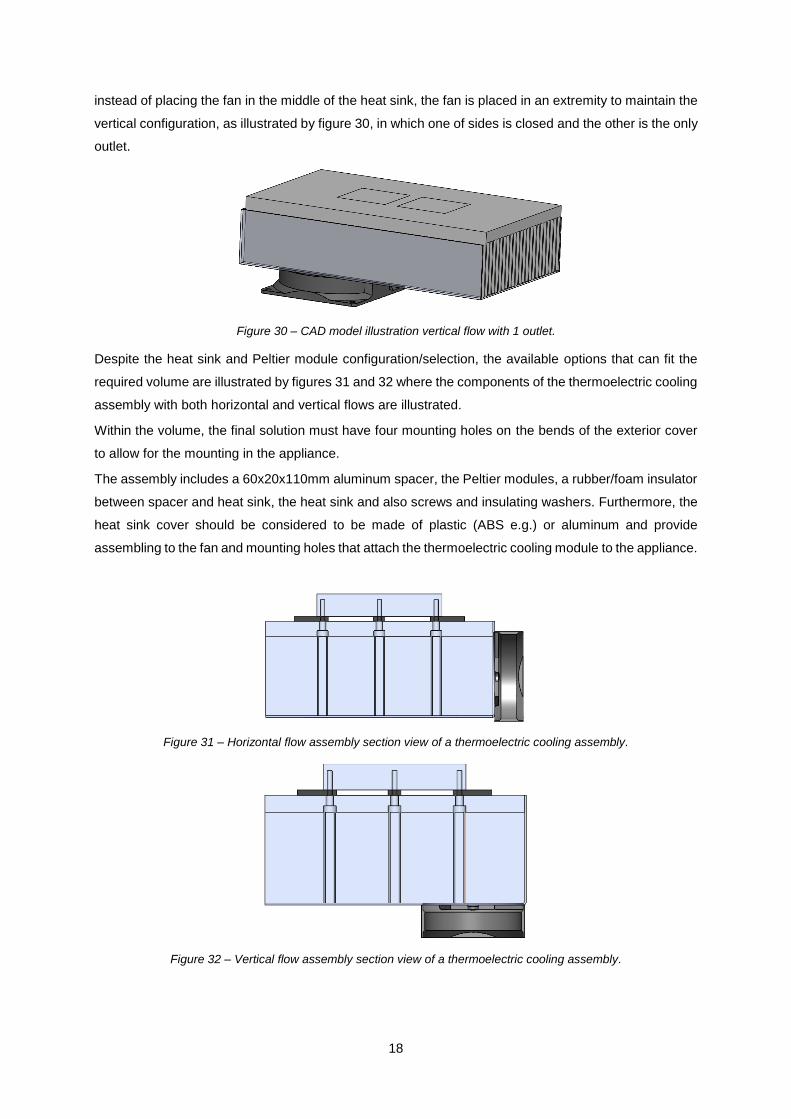
18
instead of placing the fan in the middle of the heat sink, the fan is placed in an extremity to maintain the
vertical configuration, as illustrated by figure 30, in which one of sides is closed and the other is the only
outlet.
Figure 30 – CAD model illustration vertical flow with 1 outlet.
Despite the heat sink and Peltier module configuration/selection, the available options that can fit the
required volume are illustrated by figures 31 and 32 where the components of the thermoelectric cooling
assembly with both horizontal and vertical flows are illustrated.
Within the volume, the final solution must have four mounting holes on the bends of the exterior cover
to allow for the mounting in the appliance.
The assembly includes a 60x20x110mm aluminum spacer, the Peltier modules, a rubber/foam insulator
between spacer and heat sink, the heat sink and also screws and insulating washers. Furthermore, the
heat sink cover should be considered to be made of plastic (ABS e.g.) or aluminum and provide
assembling to the fan and mounting holes that attach the thermoelectric cooling module to the appliance.
Figure 31 – Horizontal flow assembly section view of a thermoelectric cooling assembly.
Figure 32 – Vertical flow assembly section view of a thermoelectric cooling assembly.
19
3.2 Hardware selection
To build a cooling assembly, Peltier modules and some heat sinks commercially available might be
implemented. The cost reduction and available data, allow to constraint the problem variables and
search for a satisfactory project combination.
3.2.1 Peltier Modules
These thermoelectric modules originate a temperature difference when submitted to an electric current.
With appropriate heat dissipation in the hot side, it allows to reduce the temperature of a volume or
object, bellow room temperature.
The Peltier modules were introduced to context by José Pinto Ferreira (see interview in annexB2). He
explained that the electrical current intensity does not suffer from high value changes during a cooling
experience – “The current intensity value tend to vary a few decimals”. He also states that the mean
temperature of the heat sink during the experience, does not suffer significant changes. Those important
inputs provided a way to model the Peltier module behavior.
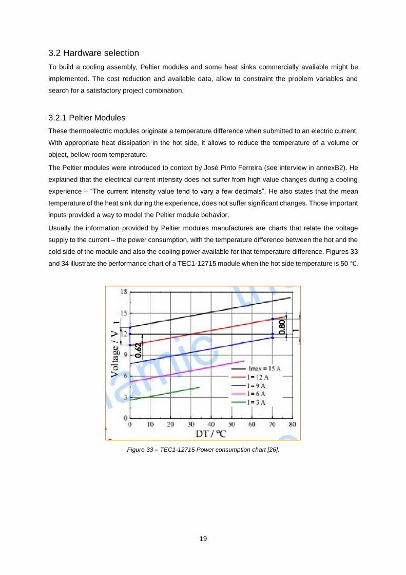
Usually the information provided by Peltier modules manufactures are charts that relate the voltage
supply to the current – the power consumption, with the temperature difference between the hot and the
cold side of the module and also the cooling power available for that temperature difference. Figures 33
and 34 illustrate the performance chart of a TEC1-12715 module when the hot side temperature is 50 ℃.
Figure 33 – TEC1-12715 Power consumption chart [26].

20
Figure 34 – TEC1-12715 Cooling rate chart [26].
Peltier modules specifications are available for two temperature values, temperature of the hot side of
25ºC and 50ºC. As the room temperature is 25ºC the specifications are imported from the 50ºC
information. To estimate the behavior of the Peltier module, one has to consider that the power supply
unit provides a steady 12V DC or 24V DC (when pairing two modules) voltage.
In the power consumption chart – figure 33, a horizontal line is drawn in the voltage value. Linear
interpolation of graphic measures allow to estimate the maximum and minimum current intensity values.
When 𝐷𝑇 = 0℃, I is approximately12𝐴 + 0.62 ∗ (15𝐴 − 12𝐴) = 13,8𝐴, whereas, when 𝐷𝑇 = 70℃, I is
approximately 9𝐴 + 0.2 ∗ (12𝐴 − 9𝐴) = 9.2𝐴. These two “working” points shall now be marked in in the
cooling rate chart – figure 34. The dashed line in figure 34 is the estimated working curve of the module.
The Peltier module may be characterized by
𝑃𝑒 = 𝑈𝑛𝑜𝑚 ∗ 𝐼𝑛𝑜𝑚 (7)
and
𝑞𝑐[𝑊] = 𝑚 ∗ (𝐷𝑇) + 𝑏 (8)
where 𝑃𝑒[𝑊] is the electrical power consumption, 𝑈𝑛𝑜𝑚[𝑉] is the voltage from the power supply unit and
𝐼𝑛𝑜𝑚[𝐴] is the average of the maximum and minimum obtained from figure 33. Eq. (8) is the functioning
curve of the Peltier module, where 𝑚 is the slop calculated from the two points obtained in figure 39 and
𝑏 is the cooling rate value when 𝐷𝑇 = 0.
The efficiency of the module decreases with the increase of the electric power and with the increase of
the temperature difference between sides. Hence, the electric power must be 80% of the maximum. The
cooling capacity decreases linearly with the temperature difference increment. For this reason, the home
appliance power supply unit is ready to receive Peltier modules to work in 24VDC or 12VDC.
The Peltier modules performance are similar between manufacturers, the data presented is from Hebei
I.T., which presents competitive prices and reliability of more than 200k hours. A brief market research

21
for suppliers revealed that prices vary according to the country of sellers where Chinese manufacturers
present highly competitive prices, justifying Hebei products as a first approach for design purposes.
The modules selected have a maximum cooling power of, at least, 84W (average cooling power of 42W).
When this condition is not verified, the junction of 2 Peltier modules is explored. Table 3 presents the
modules and configurations selected.
Table 3 – Peltier modules technical information
Peltier Module Technical Specifications Cost [USD]
TEC 1 – 12706 [26] (2 modules
in series)
𝑄𝑚𝑎𝑥 = 57𝑊 𝑉𝑚𝑎𝑥 = 14.4𝑉 𝐼𝑚𝑎𝑥 = 6.4𝑊
𝑄𝑎𝑣 = 25𝑊 𝑉𝑛𝑜𝑚 = 12𝑉 𝐼𝑛𝑜𝑚 = 4.25𝐴
7.99
TEC 1 – 12708 [27] (2 modules
in series)
𝑄𝑚𝑎𝑥 = 79𝑊 𝑉𝑚𝑎𝑥 = 17.5𝑉 𝐼𝑚𝑎𝑥 = 8.5𝐴
𝑄𝑎𝑣 = 32𝑊 𝑉𝑛𝑜𝑚 = 12𝑉 𝐼𝑛𝑜𝑚 = 5.6𝐴
8.29
TEC 1 – 12710 [28] 𝑄𝑚𝑎𝑥 = 96𝑊 𝑉𝑚𝑎𝑥 = 17.4𝑉 𝐼𝑚𝑎𝑥 = 10.5𝑊
𝑄𝑎𝑣 = 40𝑊 𝑉𝑛𝑜𝑚 = 12𝑉 𝐼𝑛𝑜𝑚 = 7.05𝐴
8.79
TEC 1 – 12715 [29] 𝑄𝑚𝑎𝑥 = 164𝑊 𝑉𝑚𝑎𝑥 = 17.2𝑉 𝐼𝑚𝑎𝑥 = 15𝑊
𝑄𝑎𝑣 = 72𝑊 𝑉𝑛𝑜𝑚 = 12𝑉 𝐼𝑛𝑜𝑚 = 11.7𝐴
27.79
The modules that are considered in this study are simple Peltier modules, with one level of semi-
conductors couples. Manufacturers offer many other solutions that might seem also reliable and tangible
for this application, but the ones chosen for this study have better cost efficiency values.
3.2.2 Heat Sinks
To build a cooling system, one of the most important features is the disposal of residual heat that every
cooling system produces. In thermoelectric cooling, and for this particular application, aluminum
extruded heat sinks might be one of the best options. The, also reviewed, bonded fins aluminum heat
sinks might also be a viable option, despite the higher production cost.
The thermal resistance, 𝑅𝑇, of a heat sink, [25] may be estimated as
𝑅𝑇 =
𝑇𝑚𝑎𝑥 − 𝑇∞
𝑃𝑑𝑖𝑠𝑠
[ ℃
𝑊] (9)
where 𝑇𝑚𝑎𝑥 is the maximum measured or estimated temperature and 𝑇∞ is the air temperature, 𝑃𝑑𝑖𝑠𝑠 is
the power that is being dissipated in those conditions.
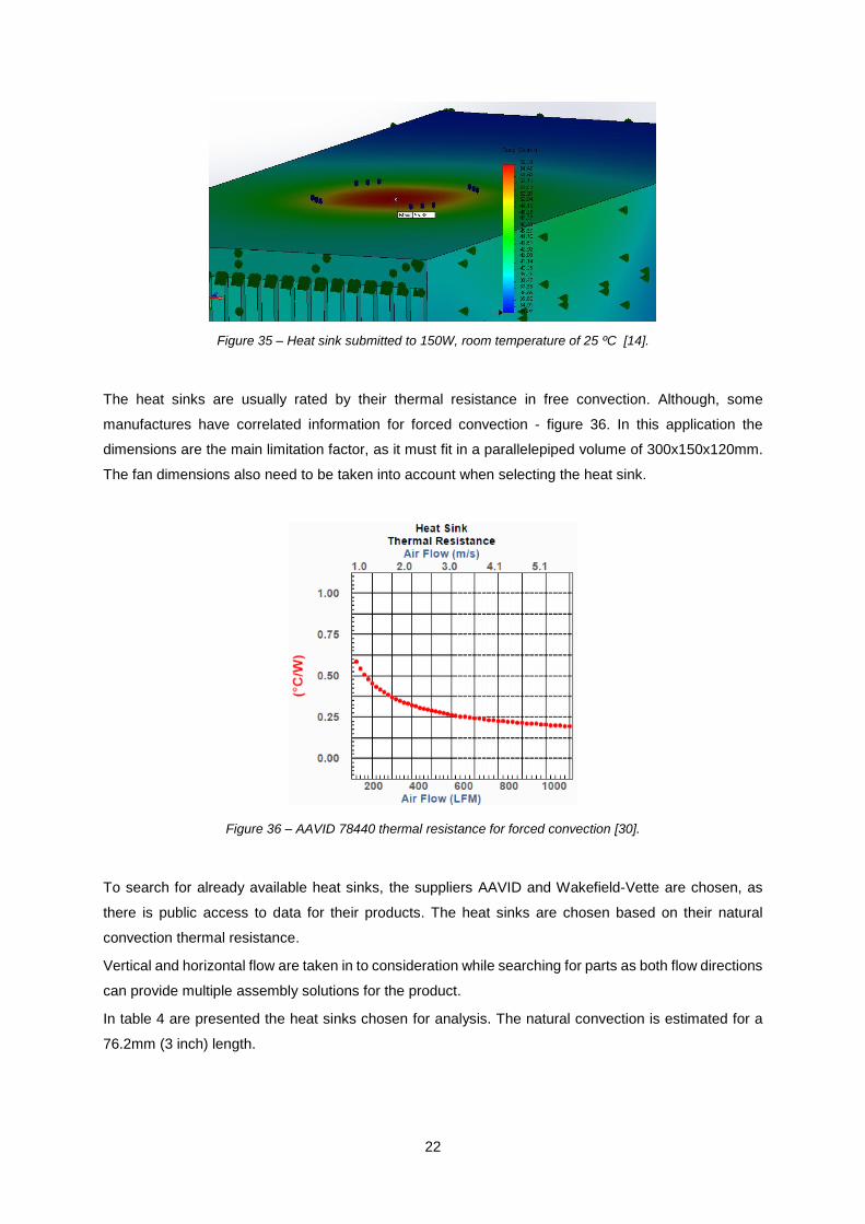
For example in the case illustrated by figure 35, that heat sink thermal resistance is about 0.2K/W. To
get this data, a known heat generation source is applied over a one square inch area, and the higher
temperature over this interface is measured.
22
Figure 35 – Heat sink submitted to 150W, room temperature of 25 ºC [14].
The heat sinks are usually rated by their thermal resistance in free convection. Although, some
manufactures have correlated information for forced convection - figure 36. In this application the
dimensions are the main limitation factor, as it must fit in a parallelepiped volume of 300x150x120mm.
The fan dimensions also need to be taken into account when selecting the heat sink.
Figure 36 – AAVID 78440 thermal resistance for forced convection [30].
To search for already available heat sinks, the suppliers AAVID and Wakefield-Vette are chosen, as
there is public access to data for their products. The heat sinks are chosen based on their natural
convection thermal resistance.
Vertical and horizontal flow are taken in to consideration while searching for parts as both flow directions
can provide multiple assembly solutions for the product.
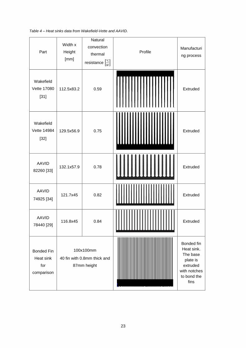
In table 4 are presented the heat sinks chosen for analysis. The natural convection is estimated for a
76.2mm (3 inch) length.
23
Table 4 – Heat sinks data from Wakefield-Vette and AAVID.
Part
Width x
Height
[mm]
Natural
convection
thermal
resistance [℃
𝑊]
Profile Manufacturi
ng process
Wakefield
Vette 17080
[31]
112.5x83.2 0.59
Extruded
Wakefield
Vette 14984
[32]
129.5x56.9 0.75
Extruded
AAVID
82260 [33] 132.1x57.9 0.78
Extruded
AAVID
74925 [34] 121.7x45 0.82
Extruded
AAVID
78440 [29] 116.8x45 0.84
Extruded
Bonded Fin
Heat sink
for
comparison
100x100mm
40 fin with 0.8mm thick and
87mm height
Bonded fin
Heat sink.
The base
plate is
extruded
with notches
to bond the
fins
24
3.2.3 Materials selection
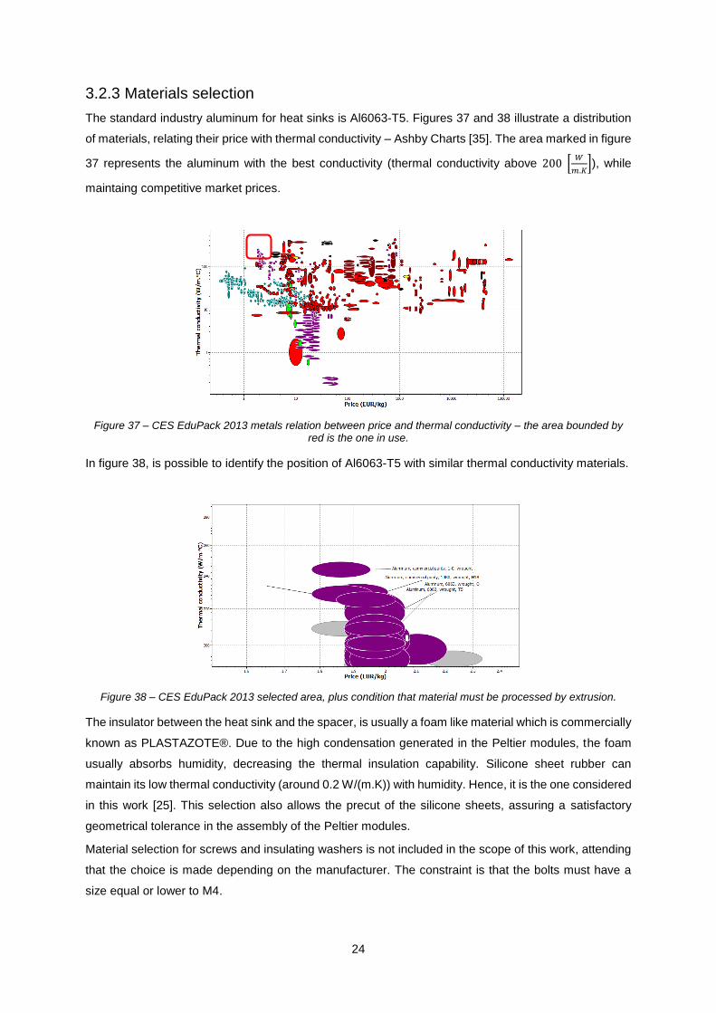
The standard industry aluminum for heat sinks is Al6063-T5. Figures 37 and 38 illustrate a distribution
of materials, relating their price with thermal conductivity – Ashby Charts [35]. The area marked in figure
37 represents the aluminum with the best conductivity (thermal conductivity above 200 [𝑊
𝑚.𝐾]), while
maintaing competitive market prices.
Figure 37 – CES EduPack 2013 metals relation between price and thermal conductivity – the area bounded by red is the one in use.
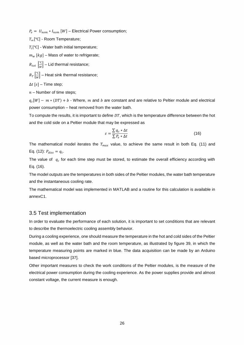
In figure 38, is possible to identify the position of Al6063-T5 with similar thermal conductivity materials.
Figure 38 – CES EduPack 2013 selected area, plus condition that material must be processed by extrusion.
The insulator between the heat sink and the spacer, is usually a foam like material which is commercially
known as PLASTAZOTE®. Due to the high condensation generated in the Peltier modules, the foam
usually absorbs humidity, decreasing the thermal insulation capability. Silicone sheet rubber can
maintain its low thermal conductivity (around 0.2 W/(m.K)) with humidity. Hence, it is the one considered
in this work [25]. This selection also allows the precut of the silicone sheets, assuring a satisfactory
geometrical tolerance in the assembly of the Peltier modules.
Material selection for screws and insulating washers is not included in the scope of this work, attending
that the choice is made depending on the manufacturer. The constraint is that the bolts must have a
size equal or lower to M4.

25
The cover, is considered to be made from aluminum, also Al6063-T5, or if economically viable from a
die casting plastic part, e.g. ABS.
Regarding the surface finish and tolerances of heat sink and the spacer, note that they depend on the
desired configuration of Peltier modules. Ferrotech, a world reference in Peltier modules manufacturing,
recommends a height tolerance of +/-0.3mm if only one Peltier module is used. If more than one is used,
this height tolerance must be +/-0.03mm, to closely match the height of all modules, ensuring a
satisfactory heat transfer [36]. All other surfaces must remain with normal process finishing and
tolerances.
3.3 Mathematical Modeling of the cooling system
In a steady condition, the functioning of a thermoelectric cooling assembly may be expressed by
𝑞𝑡 = 𝑛𝑃 ∗ 𝑃𝑒 + 𝑛𝑃 ∗ 𝑞𝑐 (10)
where 𝑞𝑡 is the total heat power removed from the Peltier modules, 𝑛𝑃 is the number of Peltier modules
in the assembly, 𝑃𝑒 is the nominal electric power consumption – see Eq. (7), and 𝑞𝑐 cooling rate of each
module - see Eq. (8).
Substituting Eq. (5) and Eq. (6) in Eq. (8), one obtains
𝑞𝑡 = 𝑛𝑃 ∗ 𝑈𝑛𝑜𝑚 ∗ 𝐼𝑛𝑜𝑚 + 𝑛𝑃 ∗ (𝑚 ∗ (𝑇𝑚𝑎𝑥 − 𝑇𝑐𝑜𝑜𝑙) + 𝑏) (11)
Hence the heat power dissipated in the heat sink may be estimated as
𝑃𝑑𝑖𝑠𝑠 =
𝑇𝑚𝑎𝑥 − 𝑇∞
𝑅𝑇
(12)
Note that the room temperature is set to be, 𝑇∞ = 25℃. If 𝑃𝑑𝑖𝑠𝑠 = 𝑞𝑡, it is possible to calculate the value
of 𝑇𝑚𝑎𝑥 and the amount of heat dissipated depending on 𝑇𝑐𝑜𝑜𝑙, the temperature of the cold side of the
Peltier module.
To estimate the amount of time needed to refrigerate the water with a set of working conditions, the
water temperature,𝑇𝑤, will vary in time, according to
𝑇𝑤 𝑖 = 𝑇𝑤 𝑖−1 −
(𝑞𝑐 − 𝑞𝑠𝑢𝑟𝑟𝑜𝑢𝑛𝑑𝑖𝑛𝑔𝑠) ∗ ∆𝑡
𝑚𝑤 ∗ 𝑐 [℃] (13)
where ∆𝑡 is the time length of the step (seconds), 𝑐 the water specific heat and i the step.
The temperature of the cold side, 𝑇𝑐𝑜𝑜𝑙, of the Peltier module may be related with the water temperature
as
𝑇𝑐𝑜𝑜𝑙 = 𝑇𝑤 − 𝑞𝑐 ∗ 𝑅𝑠𝑝𝑎𝑐𝑒𝑟 (14)
and 𝑅𝑠𝑝𝑎𝑐𝑒𝑟 is the aluminum spacer thermal resistance that may be expressed as
𝑅𝑠𝑝𝑎𝑐𝑒𝑟 =
0.02
209 ∗ (0.06 ∗ 0.11)= 0.0145 [
℃
𝑊] (15)
The model inputs are:
26
𝑃𝑒 = 𝑈𝑛𝑜𝑚 ∗ 𝐼𝑛𝑜𝑚 [𝑊] – Electrical Power consumption;
𝑇∞[℃] - Room Temperature;
𝑇𝑖[℃] - Water bath initial temperature;
𝑚𝑤 [𝑘𝑔] – Mass of water to refrigerate;
𝑅𝑡𝑜𝑡 [℃
𝑊] – Lid thermal resistance;
𝑅𝑇 [℃
𝑊] – Heat sink thermal resistance;
∆𝑡 [𝑠] – Time step;
𝑛 – Number of time steps;
𝑞𝑐[𝑊] − 𝑚 ∗ (𝐷𝑇) + 𝑏 - Where, 𝑚 and 𝑏 are constant and are relative to Peltier module and electrical
power consumption – heat removed from the water bath.
To compute the results, it is important to define 𝐷𝑇, which is the temperature difference between the hot
and the cold side on a Peltier module that may be expressed as
𝜀 =
∑ 𝑞𝑐 ∗ ∆𝑡
∑ 𝑃𝑒 ∗ ∆𝑡 (16)
The mathematical model iterates the 𝑇𝑚𝑎𝑥 value, to achieve the same result in both Eq. (11) and
Eq. (12): 𝑃𝑑𝑖𝑠𝑠 = 𝑞𝑡.
The value of 𝑞𝑐 for each time step must be stored, to estimate the overall efficiency according with
Eq. (16).
The model outputs are the temperatures in both sides of the Peltier modules, the water bath temperature
and the instantaneous cooling rate.
The mathematical model was implemented in MATLAB and a routine for this calculation is available in
annexC1.
3.5 Test implementation
In order to evaluate the performance of each solution, it is important to set conditions that are relevant
to describe the thermoelectric cooling assembly behavior.
During a cooling experience, one should measure the temperature in the hot and cold sides of the Peltier
module, as well as the water bath and the room temperature, as illustrated by figure 39, in which the
temperature measuring points are marked in blue. The data acquisition can be made by an Arduino
based microprocessor [37].
Other important measures to check the work conditions of the Peltier modules, is the measure of the
electrical power consumption during the cooling experience. As the power supplies provide and almost
constant voltage, the current measure is enough.
27
Figure 39 – Thermocouples location in the thermoelectric assembly for experience [14].
3.5.1 Material needed to test procedure
To proceed with the experiment, one needs a microprocessor, as an ARDUINO based solution that is
simple to implement is adopted. Furthermore, a set of four thermocouples, K-type, and signal amplifiers,
to measure the temperatures in the figure 39 blue points. To monitor the current consumption of the
thermoelectric assembly, one should use a current sensor, based on Hall effect.
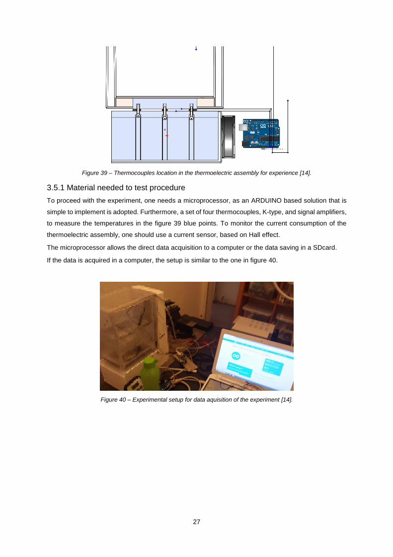
The microprocessor allows the direct data acquisition to a computer or the data saving in a SDcard.
If the data is acquired in a computer, the setup is similar to the one in figure 40.
Figure 40 – Experimental setup for data aquisition of the experiment [14].

28
4 Numerical Analysis
ANSYS Icepak is a CAE software that allows modeling of electronic system designs and conduct fluid
flow and heat transfer simulations. This reduces the product time-to-market [38]. ANSYS Icepak uses
the ANSYS Fluent computational fluid dynamics solver engine. It solves partially differential equations,
in a control volume, based on finite volume method, using a SIMPLE algorithm.
4.1 Governing Equations of Fluid Flow
The general forms of the governing equations of the fluid flow are represented in equations 17-19. They
include the compressibility and the turbulence effects as well as the source terms:
Conservation of mass:
𝜕𝜌
𝜕𝑡+ ∇. (𝜌�⃗�) = 0 (17)
For an incompressible fluid, it reduces to:
∇. �⃗� = 0 (18)
Momentum Equations:
𝜕
𝜕𝑡(𝜌�⃗�) + ∇. (𝜌�⃗��⃗�) = −∇𝑝 + ∇. (𝜏̿) + 𝜌�⃗� + �⃗� (19)
Where, 𝑝 is the static pressure, 𝜏̿ is the stress tensor, 𝜌�⃗� is the gravitational body force and �⃗� contains
other source terms that may rise from resistances or sources.
𝜏̿ = 𝜇[(∇�⃗� + ∇�⃗�𝑇) −
2
3∇. �⃗�𝐼 (20)
Where 𝜇 is the molecular viscosity, 𝐼 is the unit tensor, the second term on the right-hand side is the
effect of volume dilation.
Energy:
The energy equation can be written in terms of sensible enthalpy, ℎ:
ℎ = ∫ 𝑐𝑝𝑑𝑇
𝑇
𝑇𝑟𝑒𝑓
(21)
As
𝜕
𝜕𝑡(𝜌ℎ) + ∇. (𝜌ℎ�⃗�) = ∇. [(𝑘 + 𝑘𝑡)∇𝑇] + 𝑆ℎ (22)
Where, 𝑇𝑟𝑒𝑓 is 298.15K, 𝑘 is the molecular conductivity, 𝑘𝑡 is the conductivity due to turbulent transport,
and 𝑆ℎ is the source term and includes any volumetric heat source defined.
Since the problem is assumed to be steady state, time dependent parameters are not considered in
equations 17 to 22.
For all heat sink and selected geometries, the flow is considered to be turbulent. Turbulence models in
ANSYS Icepak are based on Reynolds averages of the governing equations. The solution variables in
the instantaneous Navier-Stokes equation are decomposed into the mean and the fluctuating
components. For velocity components:
29
𝑢𝑖 = �̅�𝑖 + 𝑢𝑖′ (23)
Where �̅�𝑖 and 𝑢𝑖′ are the mean and instantaneous velocity components (i=1,2,3).
For pressure and other scalar quantities, the method is the same:
𝜑 = �̅� + 𝜑′ (24)
Applying this conditions, will lead “Reynolds-averaged” Navier-Stokes (RANS) [39]. Those RANS, for
turbulence modeling, require that the Reynolds stresses are properly modeled. A common method
employs the Boussinesq hypothesis. Boussinesq postulated that the moment transfer caused by
turbulent eddies can be modeled with an eddy viscosity [40]. This hypothesis is used in the Spalart-
Allmaras model and the 𝑘 − 𝜀 models – first order models of one and two partially differential equations.
The disadvantage of the Boussinesq hypothesis is that it assumes 𝜇𝑡, turbulent viscosity, as an isotropic
scalar quantity, which is not strictly true.
In the scope of this work, three turbulence models are used in the numerical simulation of the fluid flow
of the heat sinks in forced-convection. These are the Spalart-Allmaras Model, the RNG 𝑘 − 𝜀 Model
enhanced with wall treatment and the Realizable 𝑘 − 𝜀 Model enhanced with wall treatment also.
The Spalart-Allmaras Model (SA) is a simple one-equation model that solves a modeled transport
equation for the kinematic eddy (turbulent) viscosity This model was designed for aerospace
applications, but provides good results for boundary layers subjected to adverse pressure gradients and
it is gaining popularity in turbomachinery applications. In ANSYS Icepak, this model is implemented to
use wall functions when the mesh resolution is not sufficiently fine. This model is usually less sensitive
to numerical erros than 𝑘 − 𝜀 models. Detailed information about the model and the mathematical
formulation can be found in [41] and [42].
Two-equation model 𝑘 − 𝜀, .(TE) [43] is the simplest “complete model” of turbulence. It determines the
solution of two independent transport equations, which allows the determination of velocity and length
scales independently. It is a popular model for industrial flow and heat transfer simulations. Is a semi-
empirical model, the derivation of the model relies on phenomenological considerations and empiricism
[40].
The RNG 𝑘 − 𝜀 model (RNG) [44], was derived using “renormalization group theory”, is similar to
standard 𝑘 − 𝜀, but has an additional term in its dissipation rate equation, that improves the accuracy
for rapidly strained flows, the effect of swirl on turbulence is included, provides an analytical formula for
turbulent Prandtl numbers, instead of constant value and provides an analytically-derived differential
formula for effective viscosity that accounts for low-Reynolds-number effects.
The Realizable 𝑘 − 𝜀 model (RTE), contains a different formulation for turbulence viscosity [41] and the
transport equation for the dissipation rate, it is derived from an exact equation for the transport of the
mean-square vorticity fluctuation. RTE is a model suited to predict the spreading rate of planar and
round jets, but also provide a superior performance for flows involving rotation, boundary layers under
strong adverse gradients, separation and recirculation.
The convective heat transfer modeling is based on Reynold’s analogy to turbulent momentum transfer,
the modeled energy equation may be expressed as:

30
𝜕
𝜕𝑡(𝜌𝐸) +
𝜕
𝜕𝜒𝑖
[𝑢𝑖(𝜌𝐸 + 𝑝)] =𝜕
𝜕𝜒𝑖
(𝑘𝑒𝑓𝑓
𝜕𝑇
𝜕𝜒𝑖
) + 𝑆ℎ (25)
Where 𝐸 is the total energy and 𝑘𝑒𝑓𝑓 is the effective conductivity. For standard TE, 𝑘𝑒𝑓𝑓 may be
expressed as equation 26, and for RNG by equation 27.
𝑘𝑒𝑓𝑓 = 𝑘 +𝑐𝑝𝜇𝑡
𝑃𝑟𝑡
(26)
𝑘𝑒𝑓𝑓 = 𝛼𝑐𝑝𝜇𝑒𝑓𝑓 (27)
Where the turbulent Prandtl number, 𝑃𝑟𝑡, is set, by default, to 0.85 and 𝛼 is the inverse effective Prandtl
number, computed using a formula derived by the renormalization group theory [44].
To get a better knowledge about the models parameters and governing equations, the reader should
consult references.
The 𝑘 − 𝜀 models are primarily valid for turbulent flows in the regions somewhat far from walls. Turbulent
flows are significantly affected by the presence of walls. The mean velocity field is affected through the
no-slip condition that has to be satisfied at the wall. Close to the wall, viscous damping reduces the
tangential velocity fluctuations, while kinematic blocking reduces the normal fluctuations. Toward the
outer part of the near-wall region, however, the turbulence is rapidly augmented by the production of
turbulence kinetic energy due to the large gradients in mean velocity.
Empirical experiments, which support the models [41] have shown that the near-wall region can be
largely subdivided into three layers. In the innermost layer, called the "viscous sublayer", the flow is
almost laminar, and the (molecular) viscosity plays a dominant role in momentum and heat or mass
transfer. In the outer layer, called the fully-turbulent layer, turbulence plays a major role. Finally, there is
an interim region between the viscous sublayer and the fully turbulent layer where the effects of
molecular viscosity and turbulence are equally important.
To more accurately resolve the flow near the wall, the enhanced two-equation models combine 𝑘 − 𝜀
models (RNG and RTE) with enhanced wall treatment (ERNG and ERTE). ANSYS Icepak combines
the two-layer model with enhanced wall functions to result in the enhanced wall treatment.
Enhanced wall treatment is a near-wall modeling method that combines a two-layer model with
enhanced wall functions. In the two-layer model, the viscosity-affected near-wall region is completely
resolved all the way to the viscous sublayer. The two-layer approach is an integral part of the enhanced
wall treatment and is used to specify both ε and the turbulent viscosity in the near-wall cells. In this
approach, the whole domain is subdivided into a viscosity-affected region and a fully-turbulent region.
The demarcation of the two regions is determined by a wall-distance-based, turbulent Reynolds number
[41].
4.2 Simulation setup and preliminary results
This step has two purposes, one is to choose a turbulence model to proceed with further studies in this
work and the other is to choose the best heat sink to fit in the thermoelectric cooling assembly.
To do so, SA, ERNG and ERTE models are compared with the same mesh for each of the six heat sinks
previously presented.
31
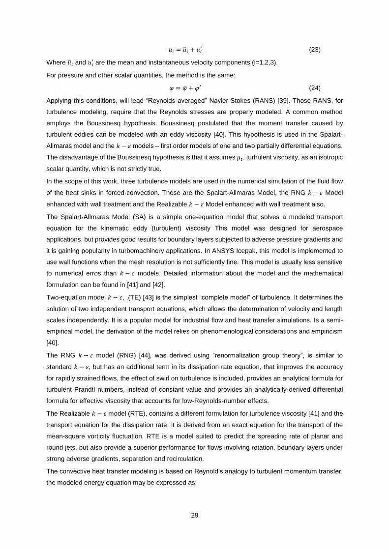
Due to geometric limitations, the extruded heat sinks have a maximum length of 200mm (value used in
calculations). For the bonded fin heat sink, the maximum plate length is 150mm, and the fins length is
120mm.
For each calculation, it is necessary to define the cabinet (physical domain), the outlet – in this work is
a clean outlet submitted to room pressure and temperature. The inlet is through a fan, depending on the
size of the heat sink, normalized computer fan diameters with inlet values of 80mm, 92mm or 120mm
may be considered. The inlet has an angular velocity of 4000RPM and inlet flows of 0.0125, 0.0250,
0.0375 and 0.0500 m3/s. The heat source implemented has an area of 40x40 mm with a power of 150W.
Figure 41 – Geometric preview of AA74925 SA125.
After the setup definition, a hexahedral based mesh is generated using ANSYS Icepak mesh quality
parameters. The minimum size volumes have to be larger than 10-12 m3 and the mesh skewness lower
value above 0.5 [40]. The same mesh was used to solve the three turbulence models.
The solving settings were set to two hundred iterations. The solution-residual values used to determine
the convergence criteria specified for the three models were: 10-5 for the flow;10-7 for the energy; and
10-7 for Joule heating.
For the ERNG and the ERTE models, the solution-residual for turbulent kinetic energy was 10-5 and for
turbulent dissipation ratio also 10-5. Table A1 in appendix, summarizes the results obtained. Not all
models achieve the convergence specified, but if the final convergence results was under 10-3, ANSYS
Icepak default, the results were considered acceptable, for this phase. The results that are not
acceptable are identified in the table by a red background.
The specification of the part indicates some details about the calculation. For example WV17080 SA, is
the heat sink profile number 17080 from Wakefield-Vette and the Spalart-Allmaras turbulence model
and if a H appears in the part name, the flow is horizontal, if not, is vertical.
The time values, were used to compare the amount of time that each turbulence model would take with
the same mesh. In a laptop with an i7 quad-core processor (@2.4GHz) and 12GB of RAM memory, the
bottleneck is the hard-drive speed of writing and reading. In these conditions, the amount of time needed
is more dependent of the number of nodes in the mesh than it is dependent of the turbulence model.
Despite the fact that BF10040H ERTE pressure values are out of scale and have no physical meaning,
the values of thermal resistance are sufficiently accurate.
32
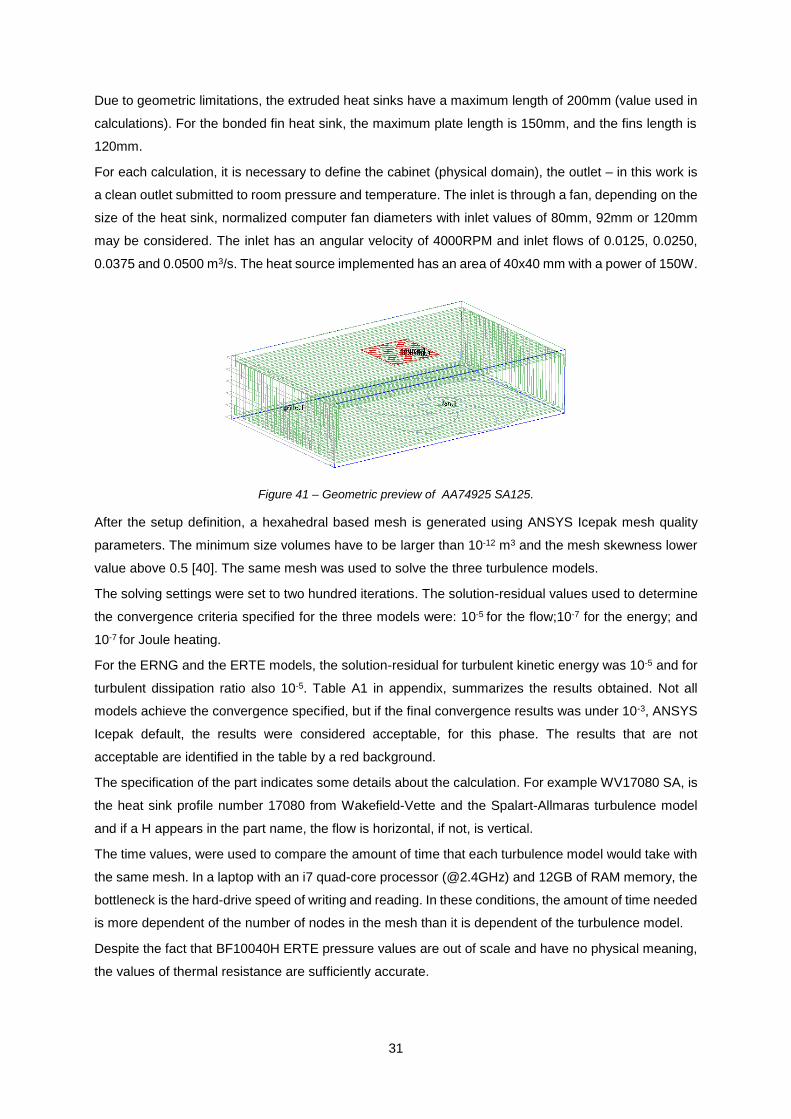
The four values of flow for each heat sink, allow to correlate a working curve for pressure drop depending
on flow rate and thermal resistance depending on flow rate. The pressure drop curve allows to intercept
with a fan working curve, giving the estimated flow rate. This value of flow rate is applied to estimate the
thermal resistance – figure 42.
Figure 42 – Fan working curve and Heat sink (WV17080H) caused pressure drop [Pa], related with the air flow [m3/s] [14].
The ERNG turbulence model, had a satisfactory and steady performance in simulations. It provided fast
convergence and reliable results. The ERNG model is chosen to proceed with more detailed calculations
for the heat sinks and configurations with the best performance.
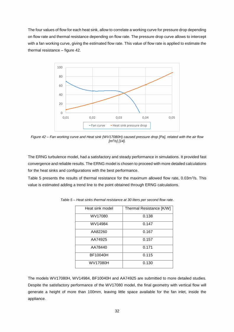
Table 5 presents the results of thermal resistance for the maximum allowed flow rate, 0.03m3/s. This
value is estimated adding a trend line to the point obtained through ERNG calculations.
Table 5 – Heat sinks thermal resistance at 30 liters per second flow rate.
Heat sink model Thermal Resistance [K/W]
WV17080 0.138
WV14984 0.147
AA82260 0.167
AA74925 0.157
AA78440 0.171
BF10040H 0.115
WV17080H 0.130
The models WV17080H, WV14984, BF10040H and AA74925 are submitted to more detailed studies.
Despite the satisfactory performance of the WV17080 model, the final geometry with vertical flow will
generate a height of more than 100mm, leaving little space available for the fan inlet, inside the
appliance.
0
20
40
60
80
100
0,01 0,02 0,03 0,04 0,05
Fan curve Heat sink pressure drop
33
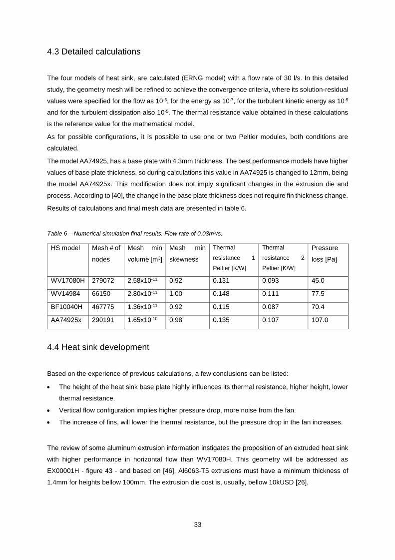
4.3 Detailed calculations
The four models of heat sink, are calculated (ERNG model) with a flow rate of 30 l/s. In this detailed
study, the geometry mesh will be refined to achieve the convergence criteria, where its solution-residual
values were specified for the flow as 10-5, for the energy as 10-7, for the turbulent kinetic energy as 10-5
and for the turbulent dissipation also 10-5. The thermal resistance value obtained in these calculations
is the reference value for the mathematical model.
As for possible configurations, it is possible to use one or two Peltier modules, both conditions are
calculated.
The model AA74925, has a base plate with 4.3mm thickness. The best performance models have higher
values of base plate thickness, so during calculations this value in AA74925 is changed to 12mm, being
the model AA74925x. This modification does not imply significant changes in the extrusion die and
process. According to [40], the change in the base plate thickness does not require fin thickness change.
Results of calculations and final mesh data are presented in table 6.
Table 6 – Numerical simulation final results. Flow rate of 0.03m3/s.
HS model Mesh # of
nodes
Mesh min
volume [m3]
Mesh min
skewness
Thermal
resistance 1
Peltier [K/W]
Thermal
resistance 2
Peltier [K/W]
Pressure
loss [Pa]
WV17080H 279072 2.58x10⁻¹¹ 0.92 0.131 0.093 45.0
WV14984 66150 2.80x10⁻¹¹ 1.00 0.148 0.111 77.5
BF10040H 467775 1.36x10⁻¹¹ 0.92 0.115 0.087 70.4
AA74925x 290191 1.65x10⁻¹⁰ 0.98 0.135 0.107 107.0
4.4 Heat sink development
Based on the experience of previous calculations, a few conclusions can be listed:
The height of the heat sink base plate highly influences its thermal resistance, higher height, lower
thermal resistance.
Vertical flow configuration implies higher pressure drop, more noise from the fan.
The increase of fins, will lower the thermal resistance, but the pressure drop in the fan increases.
The review of some aluminum extrusion information instigates the proposition of an extruded heat sink
with higher performance in horizontal flow than WV17080H. This geometry will be addressed as
EX00001H - figure 43 - and based on [46], Al6063-T5 extrusions must have a minimum thickness of
1.4mm for heights bellow 100mm. The extrusion die cost is, usually, bellow 10kUSD [26].
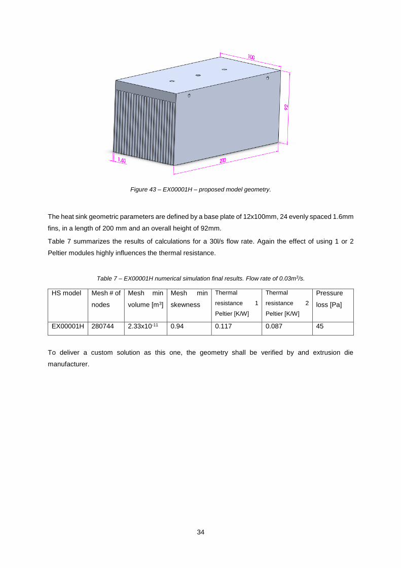
34
Figure 43 – EX00001H – proposed model geometry.
The heat sink geometric parameters are defined by a base plate of 12x100mm, 24 evenly spaced 1.6mm
fins, in a length of 200 mm and an overall height of 92mm.
Table 7 summarizes the results of calculations for a 30l/s flow rate. Again the effect of using 1 or 2
Peltier modules highly influences the thermal resistance.
Table 7 – EX00001H numerical simulation final results. Flow rate of 0.03m3/s.
HS model Mesh # of
nodes
Mesh min
volume [m3]
Mesh min
skewness
Thermal
resistance 1
Peltier [K/W]
Thermal
resistance 2
Peltier [K/W]
Pressure
loss [Pa]
EX00001H 280744 2.33x10⁻¹¹ 0.94 0.117 0.087 45
To deliver a custom solution as this one, the geometry shall be verified by and extrusion die
manufacturer.
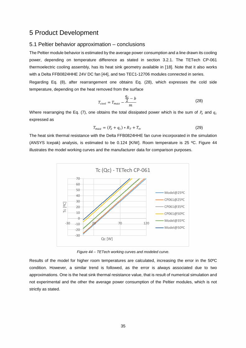
35
5 Product Development
5.1 Peltier behavior approximation – conclusions
The Peltier module behavior is estimated by the average power consumption and a line drawn its cooling
power, depending on temperature difference as stated in section 3.2.1. The TETech CP-061
thermoelectric cooling assembly, has its heat sink geometry available in [18]. Note that it also works
with a Delta FFB0824HHE 24V DC fan [44], and two TEC1-12706 modules connected in series.
Regarding Eq. (8), after rearrangement one obtains Eq. (28), which expresses the cold side
temperature, depending on the heat removed from the surface
𝑇𝑐𝑜𝑜𝑙 = 𝑇𝑚𝑎𝑥 −
𝑞𝑐
2− 𝑏
𝑚 (28)
Where rearranging the Eq. (7), one obtains the total dissipated power which is the sum of 𝑃𝑒 and 𝑞𝑐
expressed as
𝑇𝑚𝑎𝑥 = (𝑃𝑒 + 𝑞𝑐) ∗ 𝑅𝑇 + 𝑇∞ (29)
The heat sink thermal resistance with the Delta FFB0824HHE fan curve incorporated in the simulation
(ANSYS Icepak) analysis, is estimated to be 0.124 [K/W]. Room temperature is 25 ºC. Figure 44
illustrates the model working curves and the manufacturer data for comparison purposes.
Figure 44 – TETech working curves and modeled curve.
Results of the model for higher room temperatures are calculated, increasing the error in the 50ºC
condition. However, a similar trend is followed, as the error is always associated due to two
approximations. One is the heat sink thermal resistance value, that is result of numerical simulation and
not experimental and the other the average power consumption of the Peltier modules, which is not
strictly as stated.
-30
-20
-10
0
10
20
30
40
50
60
70
-30 20 70 120
Tc [
ºC]
Qc [W]
Tc (Qc) - TETech CP-061
Model@25ºC
CP061@25ºC
CP061@35ºC
CP061@50ºC
Model@35ºC
Model@50ºC
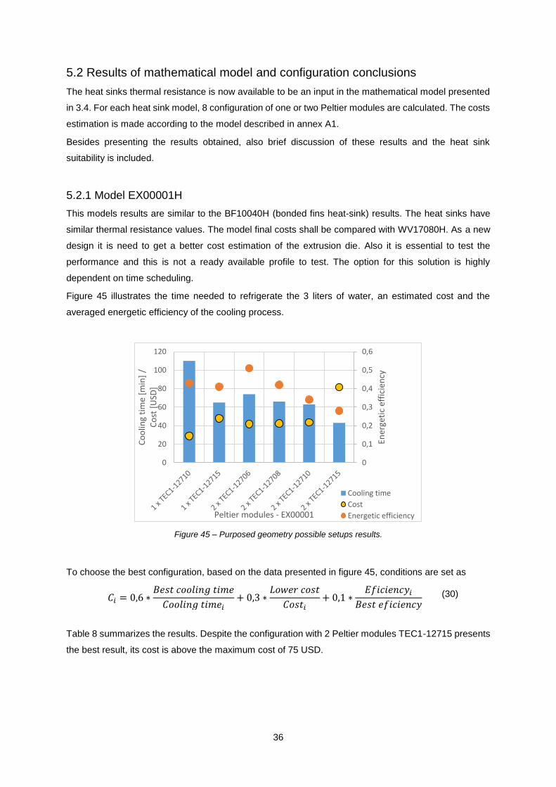
36
5.2 Results of mathematical model and configuration conclusions
The heat sinks thermal resistance is now available to be an input in the mathematical model presented
in 3.4. For each heat sink model, 8 configuration of one or two Peltier modules are calculated. The costs
estimation is made according to the model described in annex A1.
Besides presenting the results obtained, also brief discussion of these results and the heat sink
suitability is included.
5.2.1 Model EX00001H
This models results are similar to the BF10040H (bonded fins heat-sink) results. The heat sinks have
similar thermal resistance values. The model final costs shall be compared with WV17080H. As a new
design it is need to get a better cost estimation of the extrusion die. Also it is essential to test the
performance and this is not a ready available profile to test. The option for this solution is highly
dependent on time scheduling.
Figure 45 illustrates the time needed to refrigerate the 3 liters of water, an estimated cost and the
averaged energetic efficiency of the cooling process.
Figure 45 – Purposed geometry possible setups results.
To choose the best configuration, based on the data presented in figure 45, conditions are set as
𝐶𝑖 = 0,6 ∗
𝐵𝑒𝑠𝑡 𝑐𝑜𝑜𝑙𝑖𝑛𝑔 𝑡𝑖𝑚𝑒
𝐶𝑜𝑜𝑙𝑖𝑛𝑔 𝑡𝑖𝑚𝑒𝑖+ 0,3 ∗
𝐿𝑜𝑤𝑒𝑟 𝑐𝑜𝑠𝑡
𝐶𝑜𝑠𝑡𝑖+ 0,1 ∗
𝐸𝑓𝑖𝑐𝑖𝑒𝑛𝑐𝑦𝑖
𝐵𝑒𝑠𝑡 𝑒𝑓𝑖𝑐𝑖𝑒𝑛𝑐𝑦
(30)
Table 8 summarizes the results. Despite the configuration with 2 Peltier modules TEC1-12715 presents
the best result, its cost is above the maximum cost of 75 USD.
0
0,1
0,2
0,3
0,4
0,5
0,6
0
20
40
60
80
100
120
Ener
geti
c ef
fici
ency
Co
olin
g ti
me
[min
] /
Co
st [
USD
]
Peltier modules - EX00001
Cooling time
Cost
Energetic efficiency

37
Table 8 – Purposed thermoelectric assembly selection results.
When comparing the options with two TEC1-12708 and TEC1-12710, the second option, despite less
efficient, is more reliable and can maintain its performance with the increase of the room temperature.
38
6 Final remarks
As initially stated, thermoelectric cooling technologies that consist of assemblies of Peltier modules and
heat sinks have proven themselves as reliable alternatives (even though more expensive) for
laboratorial applications and small home appliances. In this work, the intent of providing a compact and
monetarily cheaper solution for a product that is initiating production with the objective of cooling 3 liters
of water, from an initial temperature of 25 ºC to a final temperature of 5 ºC, in a 2 hour time period was
successfully accomplished.
It is noted that:
The design of a thermoelectric cooling model, based in its final application allows to achieve
higher efficiency and performances, when compared to similar market available solutions, with
equivalent volumes and electric power.
The results estimated for vertical flow heat sinks are lower than expected when compared with
manufacturer data, but usually air comes from the bottom and flows through both sides. The
tested configuration has only one outlet, increasing the pressure loss induced in the fan, the
noise generated and also increasing the thermal resistance in the heat sink.
High aspect ratio heat sinks as WV17080 can perform as well as bonded fins heat sinks, but
the bonded fin option is always more compact (~1.5 times).
The setup for a thermoelectric cooling assembly is highly dependent on the working conditions,
as temperatures requirements and room temperature.
Regarding the best suitable configuration, it will highly depend on physical testing. From this
work one can conclude that a two Peltier modules configuration with TEC1-12706 can achieve
the goal of two hour with very satisfactory efficiency. The choice for that option relies in setting
a maximum room temperature threshold (around 30ºC) to guarantee minimum temperature of
5ºC on the water bath.
One other option is to consider the inclusion of heat pipes inside the heat sinks, or liquid cooling,
which will probably present higher costs, but they will highly reduce the volume occupation.
Regarding the estimated costs, an air-liquid heat exchanger must be evaluated. According to
[47] the amount of heat it can remove is related with both fan (air) flow rate, and pump (liquid)
flow rate. Values of system thermal resistance are expected to be between 0.02 and 0.10
[ºC/W].
The estimated price for these heat exchangers is between 8 and 12 USD [48], but the system
also needs a pump (costs around 15 USD) and a solid to liquid heat exchanger to connect to
the Peltier module (costs around 5 USD).
Compared with market available thermoelectric cooling assemblies, the estimated final cost of
purposed solutions is around 50 USD. A 60% batch size discount in a similar performance and
size market available solution has an estimated final cost of 190 USD [23].

39
6.1 Next steps
The heat sinks thermal resistance in the refrigeration model are for a flow rate of 30l/s, bench tests of a
constant power load on a heat sink surface, with a controlled flow rate, can provide a value of thermal
resistance to compare and correct the mathematical model – data measures of the thermoelectric
cooling assembly mounted in the kitchen appliance prototype.
Set tests to measure the Peltier modules working conditions (electrical and temperature measures).
During the refrigeration process, the electrical current, the temperature on both sides of the module, the
fan flow rate and the room temperature shall be accurately measured.
40
References
[1] G. Pahl and W. Beitz, Engineering Design A Systematic Approach. London: Springer, 1995.
[2] Robin Roj, Nils Katenbrink, “Investigation on the Application of Different Air-Cooling-Systems in a
Thermoelectric Setup”, Quick-Ohm Küpper & Co. GmbH, Unterdahl 24B, 42349 Wuppertal, Germany,
2015
[3] Mohamed Ali Rahmani, Rebei Bel Fdhila, Asa Gronqvist, Magnus Tysell, Torbjorn L. Persson,
Miroslaw Benendo, Zacharias Uvgard, “Thermal Management and Design Optimization of Heatsink for
Cooling Performance Improvement During Transient Heat Generation”, ABB AB, SE - 721 61, Västerås,
Sweden, Mälardalen University, School of Business, Society & Engineering, P.O. Box 883, SE-721 23,
Västerås, Sweden, 2014
[4] Mohamed R. Shaalan, Mohamed A. Saleh, Osama Mesalhy, Mohamed L. Elsayed, “Thermo/fluid
performance of a shielded heat sink”, Mechanical Power Engineering Department, Zagazig University,
Egypt, 2012
[5] Youmin Yu, Terrence Simon, , Tianhong Cui, “A parametric study of heat transfer in an air-cooled
heat sink enhanced by actuated plates”, Department of Mechanical Engineering, University of
Minnesota, 111 Church Street SE, Minneapolis, MN 55455, USA, 2013
[6] J. Moran and H. N. Shapiro, Fundamentals of engineering thermodynamics – 5th ed. West Sussex, England: John Wiley & Sons Inc., 2006.
[7] B. Aupoix, P.R. Spalart, “Extensions of the Spalart–Allmaras turbulence model to account for wall
roughness”, Boeing Commercial Airplane Group, P.O. Box 3707, Seattle, WA 98124, USA, 2002
[8] P. Rohdin, B. Moshfegh, “Numerical predictions of indoor climate in large industrial premises. A
comparison between different k–ε models supported by field measurements”, Division of Energy
Systems, Department of Mechanical Engineering, Linköping Institute of Technology, S -581 83
Linköping, Sweden, 2007
[9] www.cookmellow.com [Online] [Oct. 2015].
[10] Food and Drug Administration, “Food Code”, 2009, United States of America
[11] Venetum Britannicum, 1676, London, p. 176 in the 1678 edition
[12] Wikipedia-EN (2015, Sep. 21). Refrigeration [Online]. Available: https://en.wikipedia.org/wiki/Refrigeration [Oct. 01, 2015].
[13] ABC Network. “2618054-3x2-940x627.jpg” in Google search [Online]. Available: http://www.abc.net.au/news/image/2618054-3x2-940x627.jpg [Oct. 01, 2015].
[14] Paulo Quental. “Personal Image database” Lisboa: Student ,IST, ULisboa, Lisboa, Octrober. 2015
[15] Ferrotech Inc. https://thermal.ferrotec.com/technology/thermoelectric in Thermoelectric [Online]. Available: https://thermal.ferrotec.com/technology/thermoelectric [Oct. 2, 2015].
[16] K. N. Otto and K. L. Wood, Product Design: Techniques in Reverse Engineering and New Product Development, USA: Prentice Hall, 2001.
[17] Laird Inc., http://www.lairdtech.com/product-categories/thermal-management/thermoelectric-assemblies/powercool-series in Thermal Management - Powercool series [Online]. Available: http://www.lairdtech.com/product-categories/thermal-management/thermoelectric-assemblies/powercool-series [Oct. 2, 2015]
[18] TETecnhology, Inc. (2015, Sep.). “CP-061 Peltier-Thermoelectric Cold Plate Cooler” [Online]. Available: http://tetech.com/wp-content/uploads/2015/09/CP-061.pdf [Oct. 12, 2015].
[19] TETecnhology, Inc. (2015, Sep.). “CP-110 Peltier-Thermoelectric Cold Plate Cooler” [Online]. Available: http://tetech.com/wp-content/uploads/2015/09/CP-110.pdf [Oct. 12, 2015].
[20] Laird Technologies Inc. “DA PowerCool Series, DA-075-24-02” [Online]. Available: http://b7c114b8ac32968eb0a5-0034a95ea8a03cf459b9e4f7b28746f2.r86.cf3.rackcdn.com/home/brandworld/files/THR-DS-DA-075-24-02%200610.pdf [Oct. 12, 2015].
[21] Laird Technologies Inc. “DA PowerCool Series, DA-039-12-02” [Online]. Available: http://b7c114b8ac32968eb0a5-0034a95ea8a03cf459b9e4f7b28746f2.r86.cf3.rackcdn.com/home/brandworld/files/THR-DS-DA-075-24-02%200610.pdf [Oct. 12, 2015].

41
[22] Kryotherm, “SPECIFICATION OF THERMOELECTRIC COOLING ASSEMBLY 380-24-AS” [Online]. Available: http://kryothermtec.com/assets/dir2attz/Spec_380-24-AS.pdf [Oct. 3, 2015].
[23] Digikey (-). Thermoelectric assemblies [Online]. Available: http://www.digikey.com/product-search/en/fans-thermal-management/thermal-thermoelectric-peltier-assemblies/1180849?k=cooling [Oct. 01, 2015].
[24] T. L. Bergman, A. S. Lavine, F. P. Incropera, D. P. Dewitt, Fundamentas of Heat and Mass Transfer – 7th ed.. USA, John Willey & Sons, 2007
[25] CES Edupak 2013 [CD-ROM]. Granta Design Limited, 2013.
[26] Hebei IT Co. “Thermoelectric Cooler Performance Specification TEC1-12706” [Online]. Available: http://peltiermodules.com/peltier.datasheet/TEC1-12706.pdf [Oct. 2015]
[27] Hebei IT Co. “Thermoelectric Cooler Performance Specification TEC1-12708” [Online]. Available: http://peltiermodules.com/peltier.datasheet/TEC1-12708.pdf [Oct. 2015]
[28] Hebei IT Co. “Thermoelectric Cooler Performance Specification TEC1-12710” [Online]. Available: http://peltiermodules.com/peltier.datasheet/TEC1-12710.pdf [Oct. 2015]
[29] Thermonamic, (--). “Specification of Thermoelectric Module TEC1-12715” [Online]. Available: http://www.thermonamic.com/TEC1-12715-English.PDF [Oct. 2015].
[30] AAVID. “78440 Specs” [Online]. Available: http://www.aavid.com/products/extrusion-heatsinks/78440 [Oct. 2015].
[31] AAVID. “82260 Specs” [Online]. Available: http://www.aavid.com/products/extrusion-heatsinks/82260 [Oct. 2015].
[32] AAVID. “74925 Specs” [Online]. Available: http://www.aavid.com/products/extrusion-heatsinks/74925 [Oct. 2015].
[33] Wakefiel Vette. “17080 Specs” [Online]. Available: http://wvmetrics.com/work/store/partdata.php?recid=501 [Oct. 2015].
[34] Wakefiel Vette. “14984 Specs” [Online]. Available: http://wvmetrics.com/work/store/partdata.php?recid=304 [Oct. 2015].
[35] M. F. Ashby, Material Selection in Mechanical Design. Butterworth-Heinemann, 2010
[36] Ferrotech, “Thermoelectric Technical Reference — Installation of Thermoelectric Modules“ [Online]. Available: https://thermal.ferrotec.com/technology/thermoelectric/thermalRef06/ [Oct. 2015]
[37] www.arduino.cc [Online] [Oct. 2015]
[38] ANSYS Icepak User Guide [CD-ROM]. ANSYS Software, 2012.
[39] T. Saad, Turbulence Modeling for beginnersI, University of Tennessee Space Institute, USA [Online]. Available: http://www.cfd-online.com/W/images/3/31/Turbulence_Modeling_For_Beginners.pdf [Oct. 2015].
[40] François G Schmitt. About Boussinesq’s turbulent viscosity hypothesis: historical remarks and a direct evaluation of its validity. Comptes Rendus M´ecanique, Elsevier, 2007, 335 (9-10), pp.617-627.
[41] ANSYS Icepak User Guide [CD-ROM]. ANSYS Software, 2014.
[42] P. R. Spalart, S. R. Allmaras, “A One-Equation Turbulence Model for Aerodynamic Flows”, Boeing Commercial Airplane Group, Seattle, 1992.
[43] B. E. Launder and D. D. Spalding. Lectures in Mathematical Models of Turbulence. Academic Press.London. 1972.
[44] D. Choudhury. "Introduction to the Renormalization Group Method and Turbulence Modeling". Technical Memorandum TM-107, 1993.
[45] Delta, “FFB 80x80x38 MM Series datasheet” [Online]. Available: http://www.mouser.com/ds/2/632/FFB80x80x38mm-515945.pdf [Oct. 2015].
[46] Engineers Edge, “Design for Extrusion Considerations, Tolerances and Review” [Online]. Available: http://www.engineersedge.com/extrusion.htm [Oct. 2015].
[40] AAVID. “82525 Specs” [Online]. Available: http://www.aavid.com/products/extrusion-heatsinks/82525 [Oct. 2015].
[47] Overclockers. “An evaluation of the thermochill radiators” [Online]. Available: http://www.overclockers.com/an-evaluation-of-the-thermochill-radiators/ [Oct. 2015]
[48] Ebay, Prices for “Computer water cooling radiator” [Online]. Available: http://www.overclockers.com/an-evaluation-of-the-thermochill-radiators/ [Oct. 2015]

42
Annexes
Table A.1 9– ANSYS Icepak results
Part Flow rate
[m3/s]
Mesh number of
nodes
Thermal resistance
[K/W]
Pressure loss
[Pa] Time [min]
WV17080 SA 0.0125 103008 0.202 12.3 1.5
WV17080 SA 0.0250 103008 0.154 44 1.5
WV17080 SA 0.0375 103008 0.135 94.7 1.5
WV17080 SA 0.0500 103008 0.123 165 1.5
WV17080ERNG 0.0125 103008 0.189 12.8 1.5
WV17080ERNG 0.0250 103008 0.147 45.2 1.5
WV17080ERNG 0.0375 103008 0.129 97.3 1.5
WV17080ERNG 0.0500 103008 0.119 169 1.5
WV17080ERTE 0.0125 103008 0.191 12.8 1.5
WV17080ERTE 0.0250 103008 0.147 45.4 1.5
WV17080ERTE 0.0375 103008 0.129 98.2 1.5
WV17080ERTE 0.0500 103008 0.118 171 1.5
WV14984 SA 0.0125 48000 0.212 16.9 1.5
WV14984 SA 0.0250 48000 0.166 57.3 1.5
WV14984 SA 0.0375 48000 0.145 120.5 1.5
WV14984 SA 0.0500 48000 0.134 204.1 1.5
WV14984ERNG 0.0125 48000 0.203 17.3 1.5
WV14984ERNG 0.0250 48000 0.156 59.9 1.5
WV14984ERNG 0.0375 48000 0.138 125.3 1.5
WV14984ERNG 0.0500 48000 0.128 213 1.5
WV14984ERTE 0.0125 48000 0.205 17.3 1.5
WV14984ERTE 0.0250 48000 0.157 60 1.5
WV14984ERTE 0.0375 48000 0.139 125.3 1.5
WV14984ERTE 0.0500 48000 0.129 213 1.5
AA82260 SA 0.0125 423306 0.237 11.2 4
AA82260 SA 0.0250 423306 0.186 40.1 4
AA82260 SA 0.0375 423306 0.163 86.2 4
AA82260 SA 0.0500 423306 0.151 149 4
AA82260ERNG 0.0125 423306 0.228 11.2 4
AA82260ERNG 0.0250 423306 0.177 40.5 4
AA82260ERNG 0.0375 423306 0.156 87.5 4
AA82260ERNG 0.0500 423306 0.143 153 4
AA82260ERTE 0.0125 423306 0.230 11.2 4
AA82260ERTE 0.0250 423306 0.179 40.6 4
AA82260ERTE 0.0375 423306 0.157 87.6 4
AA82260ERTE 0.0500 423306 0.145 153 4
AA74925 SA 0.0125 280224 0.222 28.5 3
AA74925 SA 0.0250 280224 0.178 94.8 3
AA74925 SA 0.0375 280224 0.157 197 3
AA74925 SA 0.0500 280224 0.145 334 3
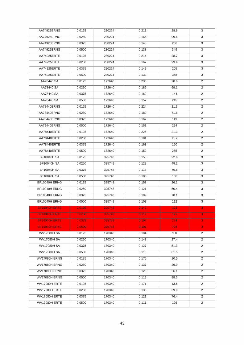
43
AA74925ERNG 0.0125 280224 0.213 28.6 3
AA74925ERNG 0.0250 280224 0.166 99.6 3
AA74925ERNG 0.0375 280224 0.148 206 3
AA74925ERNG 0.0500 280224 0.138 349 3
AA74925ERTE 0.0125 280224 0.214 28.7 3
AA74925ERTE 0.0250 280224 0.167 99.4 3
AA74925ERTE 0.0375 280224 0.149 205 3
AA74925ERTE 0.0500 280224 0.139 348 3
AA78440 SA 0.0125 172640 0.235 20.6 2
AA78440 SA 0.0250 172640 0.189 69.1 2
AA78440 SA 0.0375 172640 0.169 144 2
AA78440 SA 0.0500 172640 0.157 245 2
AA78440ERNG 0.0125 172640 0.224 21.3 2
AA78440ERNG 0.0250 172640 0.180 71.6 2
AA78440ERNG 0.0375 172640 0.162 149 2
AA78440ERNG 0.0500 172640 0.151 254 2
AA78440ERTE 0.0125 172640 0.225 21.3 2
AA78440ERTE 0.0250 172640 0.181 71.7 2
AA78440ERTE 0.0375 172640 0.163 150 2
AA78440ERTE 0.0500 172640 0.152 255 2
BF10040H SA 0.0125 325748 0.153 22.6 3
BF10040H SA 0.0250 325748 0.123 48.2 3
BF10040H SA 0.0375 325748 0.113 76.6 3
BF10040H SA 0.0500 325748 0.105 106 3
BF10040H ERNG 0.0125 325748 0.153 26.1 3
BF10040H ERNG 0.0250 325748 0.121 50.4 3
BF10040H ERNG 0.0375 325748 0.109 78.1 3
BF10040H ERNG 0.0500 325748 0.103 112 3
BF10040H ERTE 0.0125 325748 0.143 123 3
BF10040H ERTE 0.0250 325748 0.117 195 3
BF10040H ERTE 0.0375 325748 0.107 274 3
BF10040H ERTE 0.0500 325748 0.101 708 3
WV17080H SA 0.0125 170340 0.184 9.8 2
WV17080H SA 0.0250 170340 0.143 27.4 2
WV17080H SA 0.0375 170340 0.127 51.3 2
WV17080H SA 0.0500 170340 0.118 81.5 2
WV17080H ERNG 0.0125 170340 0.175 10.5 2
WV17080H ERNG 0.0250 170340 0.137 29.9 2
WV17080H ERNG 0.0375 170340 0.123 56.1 2
WV17080H ERNG 0.0500 170340 0.115 88.3 2
WV17080H ERTE 0.0125 170340 0.171 13.6 2
WV17080H ERTE 0.0250 170340 0.135 39.9 2
WV17080H ERTE 0.0375 170340 0.121 76.4 2
WV17080H ERTE 0.0500 170340 0.111 126 2
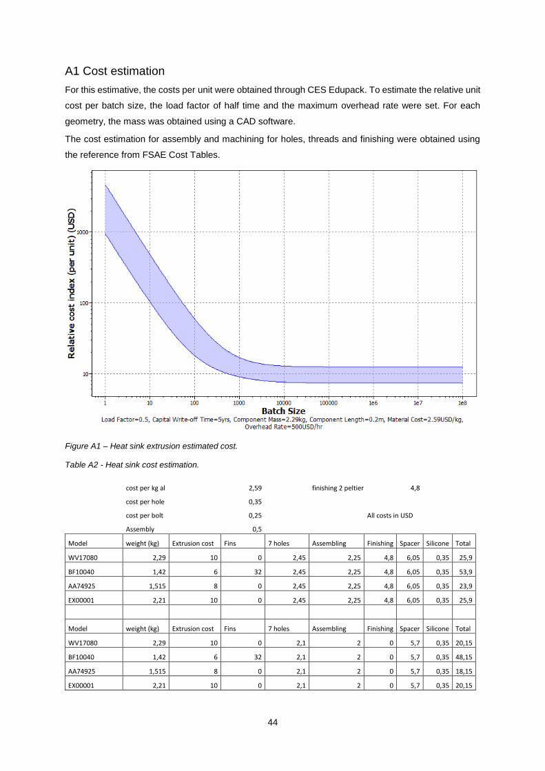
44
A1 Cost estimation
For this estimative, the costs per unit were obtained through CES Edupack. To estimate the relative unit
cost per batch size, the load factor of half time and the maximum overhead rate were set. For each
geometry, the mass was obtained using a CAD software.
The cost estimation for assembly and machining for holes, threads and finishing were obtained using
the reference from FSAE Cost Tables.
Figure A1 – Heat sink extrusion estimated cost.
Table A2 - Heat sink cost estimation.
cost per kg al 2,59 finishing 2 peltier 4,8
cost per hole 0,35
cost per bolt 0,25 All costs in USD
Assembly 0,5
Model weight (kg) Extrusion cost Fins 7 holes Assembling Finishing Spacer Silicone Total
WV17080 2,29 10 0 2,45 2,25 4,8 6,05 0,35 25,9
BF10040 1,42 6 32 2,45 2,25 4,8 6,05 0,35 53,9
AA74925 1,515 8 0 2,45 2,25 4,8 6,05 0,35 23,9
EX00001 2,21 10 0 2,45 2,25 4,8 6,05 0,35 25,9
Model weight (kg) Extrusion cost Fins 7 holes Assembling Finishing Spacer Silicone Total
WV17080 2,29 10 0 2,1 2 0 5,7 0,35 20,15
BF10040 1,42 6 32 2,1 2 0 5,7 0,35 48,15
AA74925 1,515 8 0 2,1 2 0 5,7 0,35 18,15
EX00001 2,21 10 0 2,1 2 0 5,7 0,35 20,15
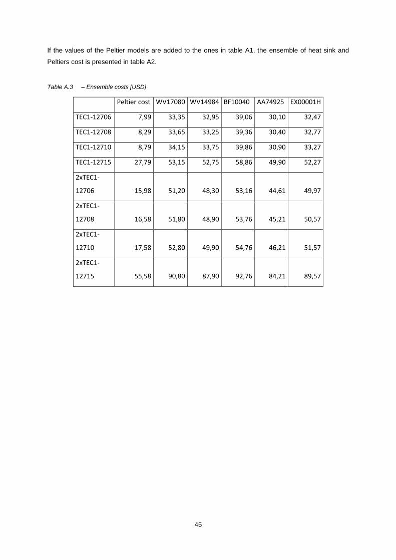
45
If the values of the Peltier models are added to the ones in table A1, the ensemble of heat sink and
Peltiers cost is presented in table A2.
Table A.3 10– Ensemble costs [USD]
Peltier cost WV17080 WV14984 BF10040 AA74925 EX00001H
TEC1-12706 7,99 33,35 32,95 39,06 30,10 32,47
TEC1-12708 8,29 33,65 33,25 39,36 30,40 32,77
TEC1-12710 8,79 34,15 33,75 39,86 30,90 33,27
TEC1-12715 27,79 53,15 52,75 58,86 49,90 52,27
2xTEC1-
12706 15,98 51,20 48,30 53,16 44,61 49,97
2xTEC1-
12708 16,58 51,80 48,90 53,76 45,21 50,57
2xTEC1-
12710 17,58 52,80 49,90 54,76 46,21 51,57
2xTEC1-
12715 55,58 90,80 87,90 92,76 84,21 89,57
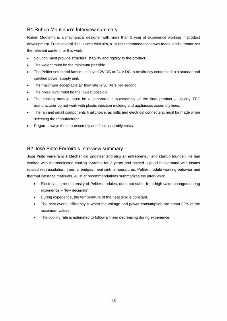
46
B1 Ruben Moutinho’s Interview summary
Ruben Moutinho is a mechanical designer with more than 5 year of experience working in product
development. From several discussions with him, a list of recommendations was made, and summarizes
the relevant content for this work:
Solution must provide structural stability and rigidity to the product.
The weight must be the minimum possible.
The Peltier setup and fans must have 12V DC or 24 V DC to be directly connected to a standar and
certified power supply unit.
The maximum acceptable air flow rate is 30 liters per second.
The noise level must be the lowest possible.
The cooling module must be a separated sub-assembly of the final product – usually TEC
manufacturer do not work with plastic injection molding and appliances assembly lines.
The fan and small components final choice, as bolts and electrical connecters, must be made when
selecting the manufacturer.
Regard always the sub-assembly and final assembly costs.
B2 José Pinto Ferreira’s Interview summary
José Pinto Ferreira is a Mechanical Engineer and also an entrepreneur and startup founder. He had
worked with thermoelectric cooling systems for 2 years and gained a good background with issues
related with insulation, thermal bridges, heat sink temperatures, Peltier module working behavior and
thermal interface materials. A list of recommendations summarizes the interviews:
Electrical current intensity of Peltier modules, does not suffer from high value changes during
experience – “few decimals”.
During experience, the temperature of the heat sink is constant.
The best overall efficiency is when the voltage and power consumption are about 80% of the
maximum values.
The cooling rate is estimated to follow a linear decreasing during experience.
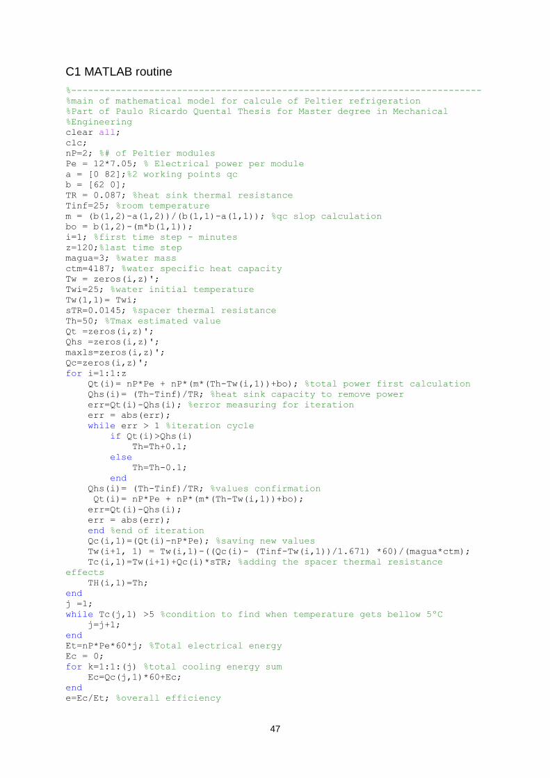
47
C1 MATLAB routine
%-------------------------------------------------------------------------- %main of mathematical model for calcule of Peltier refrigeration %Part of Paulo Ricardo Quental Thesis for Master degree in Mechanical %Engineering clear all; clc; nP=2; %# of Peltier modules Pe = 12*7.05; % Electrical power per module a = [0 82];%2 working points qc b = [62 0]; TR = 0.087; %heat sink thermal resistance Tinf=25; %room temperature m = (b(1,2)-a(1,2))/(b(1,1)-a(1,1)); %qc slop calculation bo = b(1,2)-(m*b(1,1)); i=1; %first time step - minutes z=120;%last time step magua=3; %water mass ctm=4187; %water specific heat capacity Tw = zeros(i,z)'; Twi=25; %water initial temperature Tw(1,1)= Twi; sTR=0.0145; %spacer thermal resistance Th=50; %Tmax estimated value Qt =zeros(i,z)'; Qhs =zeros(i,z)'; maxls=zeros(i,z)'; Qc=zeros(i,z)'; for i=1:1:z Qt(i)= nP*Pe + nP*(m*(Th-Tw(i,1))+bo); %total power first calculation Qhs(i)= (Th-Tinf)/TR; %heat sink capacity to remove power err=Qt(i)-Qhs(i); %error measuring for iteration err = abs(err); while err > 1 %iteration cycle if Qt(i)>Qhs(i) Th=Th+0.1; else Th=Th-0.1; end Qhs(i)= (Th-Tinf)/TR; %values confirmation Qt(i)= nP*Pe + nP*(m*(Th-Tw(i,1))+bo); err=Qt(i)-Qhs(i); err = abs(err); end %end of iteration Qc(i,1)=(Qt(i)-nP*Pe); %saving new values Tw(i+1, 1) = Tw(i,1)-((Qc(i)- (Tinf-Tw(i,1))/1.671) *60)/(magua*ctm); Tc(i,1)=Tw(i+1)+Qc(i)*sTR; %adding the spacer thermal resistance
effects TH(i,1)=Th; end j =1; while Tc(j,1) >5 %condition to find when temperature gets bellow 5ºC j=j+1; end Et=nP*Pe*60*j; %Total electrical energy Ec = 0; for k=1:1:(j) %total cooling energy sum Ec=Qc(j,1)*60+Ec; end e=Ec/Et; %overall efficiency

48
R = [j e] %--------------------------------------------------------------------------