Computational Chemistry lab

Inbal Oz

Simulation Techniques

• Introduction

• Simulation methods:

- Monte Carlo

- Molecular Dynamics

- Langevin methods

• Next lab.

Outline

Chemical Physics 446 (2015) 118–126

• When solving a single or a few molecules, electronic structure methods are typically used.

- Schrödinger equation.

- Temperature of 0 K.

- Vacuum.

- Molecules are at the ground state.

Computational Challenge

• However, the majority of chemical reactions and biologically relevant processes an are carried out in solution.

• Two major techniques for generating an ensemble:

- Monte Carlo

- Molecular dynamics

- (Langevin methods)

Generating an Ensemble

• Two major techniques for generating an ensemble:

- Monte Carlo

- Molecular dynamics

- (Langevin methods)

Generating an Ensemble

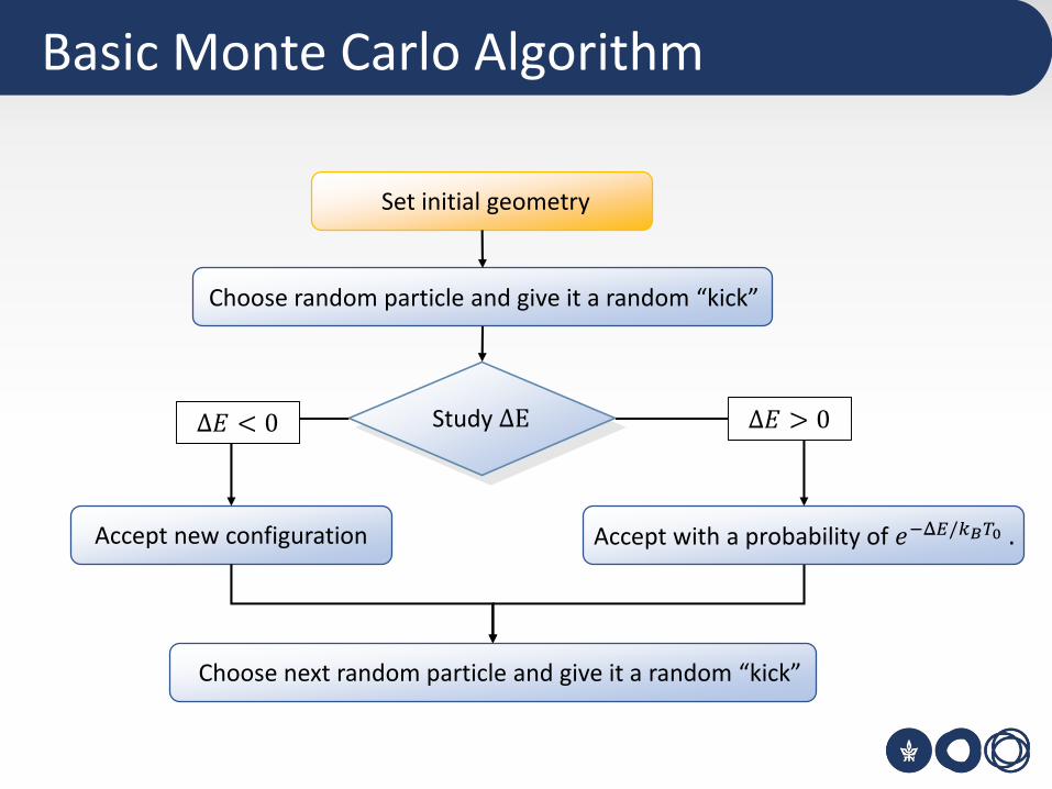
Basic Monte Carlo Algorithm

Set initial geometry

Choose random particle and give it a random “kick”

Accept new configuration

Study ΔE Δ𝐸 > 0Δ𝐸 < 0

Choose next random particle and give it a random “kick”

Accept with a probability of 𝑒−Δ𝐸/𝑘𝐵𝑇0 .

Why?

ethane

Advantages:

• Possibility of “tunnelling” between energetically

separated regions of phase space.

• It’s possible to “freeze” certain degrees of

freedom

• Requires only the ability to evaluate the energy of

the system.

Monte Carlo

Chemical Physics 446 (2015) 118–126

Disadvantages:

• limΔ𝐸→∞

𝑒−Δ𝐸/𝑘𝐵𝑇0 = 0 : the step size must be fairly small.

• Lack of time dimension and atomic velocities.

→ Not suitable for studying time-dependent phenomena or properties

depending on momentum.

• Two major techniques for generating an ensemble:

- Monte Carlo

- Molecular dynamics

- (Langevin methods)

Generating an Ensemble

• Nuclei are heavy enough that they, to a good approximation, behave as classical particles.

• Molecular Dynamics (MD) methods generate a trajectory by propagating a starting set of coordinates and velocities using Newton’s second equation.

• For each atom:

- Position (𝑟).

- Momentum (𝑚 + 𝑣).

- Charge (𝑞).

- Bond information (neighbors, bond angles, etc.).

Molecular Dynamics

Computational Challenge

• To discover the trajectory, we need to know the potential affecting each atom.

- Bonded neighbors.

- Non-Bonded atoms.

From Potential to Movement

bondednonbonded EERV −+=)(

Bonded Atoms

Stretch Bend Rotate

bondalongrotatebendanglestretchbondbonded EEEE −−−− ++=

MM mimimizes the potential energy given by a force field.MD is the actual algorithmic solving of newton's equations to see motion.

• The Non-bonded interaction includes:

- Van der Waals Potential.

- Electrostatic Potential.

Non-Bonded Atoms

• Usually modeled using the Lennard-Jones potential.

Van der Waals Potential

Lennard Jones

• Same charges are repelled, while opposite charges are

attracted.

Electrostatic Potential

• Combining the van der Waals potential and the electrostatic potential gives us the non-bonded potential.

The Non-Bonded Potential

ticelectrostaWaalsdervanbondednon EEE += −−−

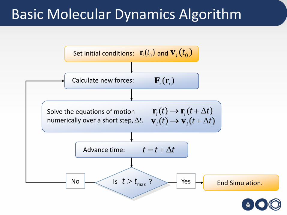
Basic Molecular Dynamics Algorithm

Set initial conditions: and)( 0tir )( 0tiv

Calculate new forces: )( ii rF

Solve the equations of motionnumerically over a short step, .

)()( ttt ii +→ rr)()( ttt ii +→ vvt

ttt +=Advance time:

Is ?maxtt End Simulation.No Yes

Some Important Concepts

• An atom moving out of

boundary comes back

from the other side.

• Large enough to include

the molecule itself.

• The size of the

computational cell should

be larger than 2𝑅𝑐𝑢𝑡.

Periodic boundary conditions

cutR

• Solvent molecules: computational burden.

• Our simulation space has certain boundaries: cell.

• All atoms in the computational cell are replicated throughout space to form an infinite lattice.

• The name and inspiration come from annealing in metallurgy.

Simulated Annealing

Bath temperature

Time step

heating

equilibration

cooling

Simulated Annealing: Example

The total energy increases.

Dynamics simulation for Alanine (heating and run phase at 300𝐾).

The temperature plot merged with the kinetic energy.

The potential energy mirrors the kinetic energy.

• Deterministic simulations - the output is fully determined by the

parameter values and the initial conditions.

• Stochastic simulations - possess some inherent randomness.

Deterministic vs. Stochastic

3 + 3 = ?

• A stochastic process is said to be ergodic if its statistical properties can be

deduced from a single, sufficiently long, random sample of the process.

→A time average over a single particle is equivalent to an average of a large

number of particles at any given time snapshot.

• Most processes in nature are ergodic.

• Example of a non-ergodic process: two coins, one fair and the other has two

heads. Choosing first one coin and then perform a sequence of independent

tosses.

Ergodic Process

Time averaging Ensemble averaging

Molecular Dynamics

• Deterministic (in principle).

• Time averaging. (sec. 4d)

Molecular Dynamics vs. Monte Carlo

Monte Carlo

• Stochastic.

• Ensemble averaging.

Ensemble Type

• A simulation can be characterized by quantities such as volume (𝑉),

pressure (𝑃), total energy (𝐸), temperature (𝑇), number of particles (𝑁),

chemical potential (𝜇), etc., but not all of these are independent.

- For a constant 𝑁, either the 𝑉 or the 𝑃 can be fixed, but not both.

- A constant 𝜇 is incomemensurable with a constant 𝑁.

• The ensemble is labelled according to the fixed quantities, with the

remainder being derived from the simulation data, and thus displaying a

statistical fluctuation.

Ensemble Type

• An MC simulation uses 𝑇 as the parameter for deciding acceptance or

rejection of trial moves (𝑒−Δ𝐸/𝑘𝐵𝑇0)

→ naturally of the 𝑁𝑉𝑇 type.

• An MD simulation (Langevin), on the other hand, preserves 𝐸 and is

therefore naturally of the 𝑁𝑉𝐸 type.

Molecular Dynamics vs. Monte Carlo

• Two major techniques for generating an ensemble:

- Monte Carlo

- Molecular dynamics

- (Langevin methods)

Generating an Ensemble

• Molecular dynamics methods generate detailed information about all the

particles in the system.

• In some cases, the major interest is in the dynamics of a single molecule.

Then, the surrounding molecules can be modelled by only including the

average interactions.

𝑚𝑑2𝒓

𝑑𝑡2= 𝑭𝑖𝑛𝑡𝑟𝑎 − 𝜁

𝑑𝒓

𝑑𝑡+ 𝑭𝑟𝑎𝑛𝑑𝑜𝑚

→ The Langevin equation of motion gives rise to stochastic dynamics.

Langevin methods

• Explicit solvation - method that uses individual solvent molecules.

- Better physical behavior.

- Computationally demanding.

• Implicit solvation - method to represent solvent as a continuous medium instead of individual “explicit” solvent molecules

- Cheaper.

- Less physical.

Explicit vs. Implicit Solvent

• You will simulate the Dynamic and Equilibrium behavior of Alanine zwitterions.

• Step 1: creation of an isolated Alanine zwitterion and measuring its properties.

- Molecular mechanics, AMBER force field.

• Step 2: Solvating the Structure.

- Geometry optimization, MM.

- Energy: lower or higher than in vacuum?

Next lab

• Step 3: Superposition.

- What are the significant changes?

• Step 4: Molecular Dynamics: simulated annealing

- Simulated annealing.

- Reoptimizing the new structure.

- Did you get a smaller energy value?

• Step 5: Langevin and Monte Carlo Simulations

- Compare.

Next lab

• Monte Carlo

• Molecular Dynamics

- Periodic boundary conditions

- Simulated annealing

- Deterministic vs. Stochastic

• Langevin methods

- Explicit vs. Implicit Solvent

• Next lab calculations.

Summary