thermodynamics: four laws that move the universe · pdf filephysics science & mathematics...

PhysicsScience & Mathematics

TopicSubtopic

Professor Jeffrey C. GrossmanMaassachusetts Institute of Technollooggy

Thermodynamics: Four Laws That Move the UniverseCouurse Guidebook

ute of Technoologogy

PUBLISHED BY:

THE GREAT COURSESCorporate Headquarters

4840 Westfields Boulevard, Suite 500Chantilly, Virginia 20151-2299

Phone: 1-800-832-2412Fax: 703-378-3819

www.thegreatcourses.com

Copyright © The Teaching Company, 2014

Printed in the United States of America

This book is in copyright. All rights reserved.

Without limiting the rights under copyright reserved above,no part of this publication may be reproduced, stored in

or introduced into a retrieval system, or transmitted, in any form, or by any means

(electronic, mechanical, photocopying, recording, or otherwise), without the prior written permission of

The Teaching Company.

i

Jeffrey C. Grossman, Ph.D.Professor in the Department of Materials

Science and Engineering Massachusetts Institute of Technology

Professor Jeffrey C. Grossman is a Professor in the Department of Materials Science and Engineering at the Massachusetts Institute

of Technology. He received his B.A. in Physics from Johns Hopkins University in 1991 and

his M.S. in Physics from the University of Illinois at Urbana-Champaign in 1992. After receiving his Ph.D. in Physics in 1996 from the University of Illinois at Urbana-Champaign, he performed postdoctoral work at the University of California, Berkeley, and was one of five selected from 600 to be a Lawrence Fellow at the Lawrence Livermore National Laboratory. During his fellowship, he helped to establish their research program in nanotechnology and received both the Physics Directorate Outstanding Scientific Achievement Award and the Science and Technology Award.

Professor Grossman returned to UC Berkeley as director of a nanoscience center and head of the Computational Nanoscience research group, which he founded and which focuses on designing new materials for energy applications. He joined the MIT faculty in the summer of 2009 and leads a research group that develops and applies a wide range of theoretical and experimental techniques to understand, predict, and design novel materials with applications in energy conversion, energy storage, and clean water.

Examples of Professor Grossman’s current research include the development of new, rechargeable solar thermal fuels, which convert and store the Sun’s energy as a transportable fuel that releases heat on demand; the design of new membranes for water purification that are only a single atom thick and lead to substantially increased performance; three-dimensional photovoltaic panels that when optimized deliver greatly enhanced power per area footprint of land; new materials that can convert waste heat directly into electricity; greener versions of one of the oldest and still most widely used building

ii

materials in the world, cement; nanomaterials for storing hydrogen safely and at high densities; and the design of a new type of solar cell made entirely out of a single element.

As a teacher, Professor Grossman promotes collaboration across disciplines to approach subject matter from multiple scientific perspectives. At UC Berkeley, he developed two original classes: an interdisciplinary course in modeling materials and a course on the business of nanotechnology, which combined a broad mix of graduate students carrying out cutting-edge nanoscience research with business students eager to seek out exciting venture opportunities. At MIT, he developed two new energy courses, taught both undergraduate and graduate electives, and currently teaches a core undergraduate course in thermodynamics.

To further promote collaboration, Professor Grossman has developed entirely new ways to encourage idea generation and creativity in interdisciplinary science. He invented speedstorming, a method of pairwise idea generation that works similarly to a round-robin speed-dating technique. Speedstorming combines an explicit purpose, time limits, and one-on-one encounters to create a setting where boundary-spanning opportunities can be recognized, ideas can be generated at a deep level of interdisciplinary specialty, and potential collaborators can be quickly assessed. By directly comparing speedstorming to brainstorming, Professor Grossman showed that ideas from speedstorming are more technically specialized and that speedstorming participants are better able to assess the collaborative potential of others. In test after test, greater innovation is produced in a shorter amount of time.

Professor Grossman is a strong believer that scientists should teach more broadly—for example, to younger age groups, to the general public, and to teachers of varying levels from grade school to high school to community college. To this end, he has seized a number of opportunities to perform outreach activities, including appearing on television shows and podcasts; lecturing at public forums, such as the Exploratorium, the East Bay Science Cafe, and Boston’s Museum of Science; developing new colloquia series with Berkeley City College; and speaking to local high school chemistry teachers about energy and nanotechnology.

iii

The recipient of a Sloan Research Fellowship and an American Physical Society Fellowship, Professor Grossman has published more than 110 scientific papers on the topics of solar photovoltaics, thermoelectrics, hydrogen storage, solar fuels, nanotechnology, and self-assembly. He has appeared on a number of television shows and podcasts to discuss new materials for energy, including PBS’s Fred Friendly Seminars, the Ecopolis program on the Discovery Channel’s Science Channel, and NPR’s On Point with Tom Ashbrook. He holds 18 current or pending U.S. patents.

Professor Grossman’s previous Great Course is Understanding the Science for Tomorrow: Myth and Reality. ■

iv

Table of Contents

LECTURE GUIDES

Professor Biography ............................................................................ iCourse Scope .....................................................................................1

INTRODUCTION

LECTURE 1Thermodynamics—What’s under the Hood ........................................5

LECTURE 2Variables and the Flow of Energy .....................................................12

LECTURE 3Temperature—Thermodynamics’ First Force ...................................19

LECTURE 4Salt, Soup, Energy, and Entropy ......................................................26

LECTURE 5The Ideal Gas Law and a Piston ......................................................32

LECTURE 6Energy Transferred and Conserved .................................................38

LECTURE 7Work-Heat Equivalence ....................................................................45

LECTURE 8Entropy—The Arrow of Time ............................................................52

LECTURE 9The Chemical Potential ....................................................................59

LECTURE 10Enthalpy, Free Energy, and Equilibrium ...........................................65

Table of Contents

v

LECTURE 11Mixing and Osmotic Pressure...........................................................71

LECTURE 12How Materials Hold Heat ..................................................................77

LECTURE 13How Materials Respond to Heat .......................................................83

LECTURE 14Phases of Matter—Gas, Liquid, Solid...............................................90

LECTURE 15Phase Diagrams—Ultimate Materials Maps .....................................97

LECTURE 16Properties of Phases ......................................................................103

LECTURE 17To Mix, or Not to Mix? .....................................................................110

LECTURE 18Melting and Freezing of Mixtures ...................................................116

LECTURE 19The Carnot Engine and Limits of Efficiency....................................123

LECTURE 20More Engines—Materials at Work ..................................................129

LECTURE 21The Electrochemical Potential ........................................................135

LECTURE 22Chemical Reactions—Getting to Equilibrium..................................141

LECTURE 23The Chemical Reaction Quotient....................................................147

Table of Contents

vi

LECTURE 24The Greatest Processes in the World .............................................154

SUPPLEmENTaL maTERIaL

Bibliography ....................................................................................161

vii

This series of lectures is intended to increase your understanding of the principles of thermodynamics. These lectures include experiments in the field of thermodynamics, performed by an experienced professional. These experiments may include dangerous materials and are conducted for informational purposes only, to enhance understanding of the material.

WARNING: THE EXPERIMENTS PERFORMED IN THESE LECTURES ARE DANGEROUS. DO NOT PERFORM THESE EXPERIMENTS ON YOUR OWN. Failure to follow these warnings could result in injury or death.

The Teaching Company expressly DISCLAIMS LIABILITY for any DIRECT, INDIRECT, INCIDENTAL, SPECIAL, OR CONSEQUENTIAL DAMAGES OR LOST PROFITS that result directly or indirectly from the use of these lectures. In states which do not allow some or all of the above limitations of liability, liability shall be limited to the greatest extent allowed by law.

Disclaimer

1

Scope:

In this course on thermodynamics, you will study a subject that connects deep and fundamental insights from the atomic scale of the world all the way to the highly applied. Thermodynamics has been pivotal for most of

the technologies that have completely revolutionized the world over the past 500 years.

The word “thermodynamics” means “heat in motion,” and without an understanding of heat, our ability to make science practical is extremely limited. Heat is, of course, everywhere, and putting heat into motion was at the core of the industrial revolution and the beginning of our modern age. The transformation of energy of all forms into, and from, heat is at the core of the energy revolution and fundamentally what makes human civilization thrive today.

Starting from explaining the meaning of temperature itself, this course will cover a massive amount of scientific knowledge. Early on, you will learn the crucial variables that allow us to describe any system and any process. Sometimes these variables will be rather intuitive, such as in the case of pressure and volume, while other times they will be perhaps not so intuitive, as in the case of entropy and the chemical potential. Either way, you will work toward understanding the meaning of these crucial variables all the way down to the scale of the atom and all the way up to our technologies, our buildings, and the planet itself. And you will not stop at simply learning about the variables on their own; rather, you will strive to make connections between them.

Once you have a solid understanding of the different variables that describe the world of thermodynamics, you will move on to learn about the laws that bind them together. The first law of thermodynamics is a statement of conservation of energy, and it covers all of the different forms of energy possible, including thermal energy. When you learn the first law, you will discover the many different ways in which energy can flow into or out of a

Thermodynamics: Four Laws That move the Universe

Scop

e

2

material. By taking a look under the hood of materials and peering across vast length and time scales, you will learn that at the fundamental level, for the energy stored in the material itself, all energy flows are equivalent.

You will learn that internal energy represents a kind of energy that is stored inside of a material and that it can tell us how that material holds onto energy from heat and responds to changes in temperature. In addition, you will learn how a change in temperature represents a crucial driving force for heat to flow—a concept also known as the zeroth law of thermodynamics.

From the first law and your knowledge of the internal energy, you will understand that performing work on a system—for example, applying a pressure or initiating a reaction—is entirely equivalent to adding heat. This is one of the fundamental pillars of thermodynamics. And armed with this knowledge, you will see that there are many different ways to manipulate the properties of materials and that you can adapt your processing techniques to whatever is most convenient given the tools you have on hand.

You will learn that vast amounts of heat can be generated not just by lighting fire, but also by other means, such as the friction of two pieces of metal rubbing together. And by understanding the relationships between the basic variables pressure, temperature, volume, and mass, you will learn how heat can go the other way, converting into some form of useful work. For example, taking advantage of the fact that heat makes a gas expand, which in turn can be used to push on a piston, you will learn about how the very first engines were made.

As you explore thermodynamics beyond the driving force and corresponding response of a material, you will learn what it is that governs when and why the system stops being driven. In other words, you will learn why a system comes to equilibrium. This means that, given any set of external conditions—such as temperature, pressure, and volume—on average, the system no longer undergoes any changes. The concept of equilibrium is so important in thermodynamics that a good portion of the early lectures of the course will be dedicated to explaining it. But it is not until the lecture on entropy and the second law of thermodynamics that you discover just how to find this special equilibrium place.

3

As you learn about the second law, you will understand just why it is that thermodynamics is the subject that treats thermal energy on an equal footing with all of the other forms: The reason it is able to do so has to do with entropy. You will be learning a lot about entropy throughout this course because it is of absolutely fundamental importance to this subject. Entropy is the crucial link between temperature and thermal energy. It is a way to quantify how many different ways there are to distribute energy, and as you will learn, it is the foundation for the second law of thermodynamics.

By understanding entropy, you will gain an intuitive sense for the connectedness of thermal energy to all other forms of energy, and you will understand why a perpetual-motion machine can never exist. Entropy offers nothing less than the arrow of time, because it is the thermodynamic variable that provides a way to predict which direction all processes will occur. And you will learn that like temperature, entropy can have an absolute minimum value, as stated in the third law of thermodynamics.

Once you have learned these laws, you will be able to apply them to the understanding of a wide range of properties and processes—for example, how materials change their phase between gas, liquid, and solid in many different ways and sometimes even possess completely new phases, as in the case of a supercritical fluid. You will learn that when two different materials are mixed together, the phase diagram provides the ultimate materials map and can help navigate through the immense complexity of mixtures.

You will learn about heat engines and discover that while work can make heat with 100 percent efficiency, heat cannot do work with 100 percent efficiency. It’s the Carnot limit that tells us that the absolute best a heat engine can ever achieve is dependent on a temperature difference.

You will learn how other types of work—including magnetism, surface tension, phase change, and entropy itself—can be used to make stuff move. And beyond these highlights, you will learn many other foundational thermodynamic concepts that are critical pillars of the science and engineering of modern times, including eutectic melting; osmotic pressure; the electrochemical cell; and that beautiful moment for a material where all

Scop

e

4

three phases coexist, called the triple point; along with many, many other important phenomena.

In this course, you will learn how the four laws of thermodynamics will continue to provide the foundation of science technology into the future, for any single aspect of our lives where a material is important. ■

5

Thermodynamics—What’s under the HoodLecture 1

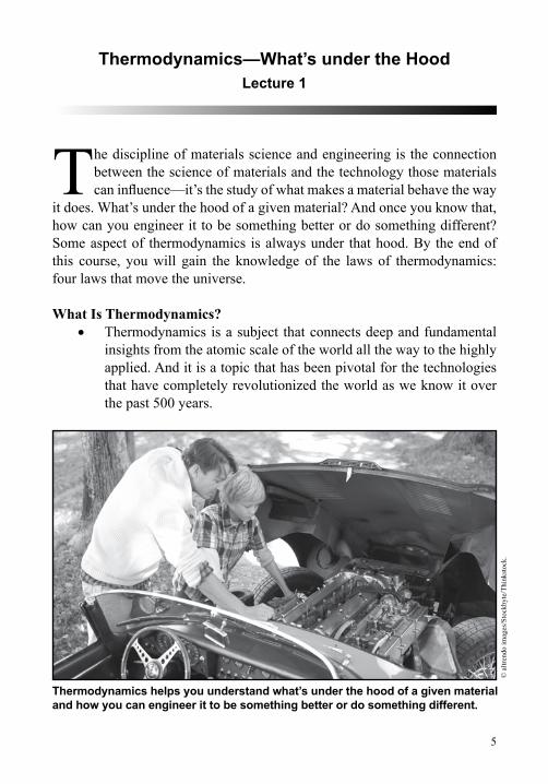
The discipline of materials science and engineering is the connection between the science of materials and the technology those materials can influence—it’s the study of what makes a material behave the way

it does. What’s under the hood of a given material? And once you know that, how can you engineer it to be something better or do something different? Some aspect of thermodynamics is always under that hood. By the end of this course, you will gain the knowledge of the laws of thermodynamics: four laws that move the universe.

What Is Thermodynamics?• Thermodynamics is a subject that connects deep and fundamental

insights from the atomic scale of the world all the way to the highly applied. And it is a topic that has been pivotal for the technologies that have completely revolutionized the world as we know it over the past 500 years.

Thermodynamics helps you understand what’s under the hood of a given material and how you can engineer it to be something better or do something different.

© a

ltren

do im

ages

/Sto

ckby

te/T

hink

stoc

k.

6

Lect

ure

1: T

herm

odyn

amic

s—W

hat’s

und

er th

e H

ood

• Perhaps the single most important differentiator for this subject is the prefix “thermo,” which means “heat”; it is the fundamental understanding of heat and temperature and, ultimately, entropy that separates this subject from all others.

• The word “thermodynamics” means “heat in motion,” and without an understanding of heat, our ability to make science practical is extremely limited. Heat is everywhere, and putting heat into motion is at the core of the industrial revolution and the beginning of our modern age. The transformation of energy of all forms into, and from, heat is at the core of the energy revolution and fundamentally what makes human civilization thrive today.

Rebuilding the World• What if all the buildings were leveled, the cars and roads were

gone, hospitals disappeared, and electricity was only found in lightning strikes? Basically, what if nothing were here? How would we rebuild our world? What would the challenges be? What tools would we need? What knowledge would we need?

• The place to start, in order to answer such questions, is to ask what the variables are in the first place. What are the “givens”? That is, what are the things that we know about, the things that we have? What are the things that we may not have but need to know about? These are the variables.

• In our effort to rebuild the world, we would ask what raw materials we could find, plus the different forms of energy we would be able to harness to manipulate those ingredients. These energies could include heat, or mechanical forces, or chemical reactions, as examples.

• Once we knew what the variables were, next we would need to know how those variables interact with one another. In other words, how do materials respond to their environment? How does one form of energy change when another form of energy is introduced? What is the interplay between energy of all forms and matter?

7

• The answers to these questions can be found in thermodynamics, which is the subject that holds the key to understanding how energy in all of its forms—including heat—changes the nature of the materials that make up the world.

• Without understanding these relationships, we could not rebuild our world. We would not be able to make an engine that turns heat into mechanical work; we would not be able to make electricity from spinning turbines.

• So, how would we begin? First, we would need to get a sense of what the variables are that we can control. These variables include temperature and pressure, the volume or mass of a substance, the phase of the material (which would mean working with the material as a gas, liquid, or solid), and the chemistry itself.

• Then, we would start varying the properties with respect to one another to see what happens. We would try to vary just a few variables at a time, while holding as many of the other ones fixed. This is what scientists and engineers did to lay the foundations of thermodynamics.

• We’ll develop a strong sense for each of these crucial variables and learn the relationships between them. We’ll build our knowledge base starting with the properties of materials when they’re in a single phase, like a gas, and then we’ll learn how and why materials can change phase as a function of their environment.

• But just knowing the variables is not enough to build something useful, which is why, once we have a solid understanding of the different variables of thermodynamics, we will move on to learn about the law that binds them all together. The first law of thermodynamics is a statement of conservation of energy, and it covers all of the different forms of energy possible, including thermal energy.

8

Lect

ure

1: T

herm

odyn

amic

s—W

hat’s

und

er th

e H

ood

• At that stage of knowledge needed in our attempt to rebuild the world, we would have a fantastic grasp of the different ways in which energy can flow into or out of a material. By taking a look under the hood of materials and peering across vast length and time scales, we’ll learn that at the fundamental level, for the energy stored in the material itself, all energy flows are equivalent.

• We would see that performing work, such as applying a pressure or initiating a reaction, is entirely equivalent to adding heat. This is one of the fundamental pillars of thermodynamics, and it is captured in the first law.

• And armed with that knowledge, we would learn that there are many ways to manipulate the properties of materials and that we can adapt our processing techniques to whatever is most convenient, given the tools we have on hand.

• We would also be able to experiment with the trading back and forth between heat and work. We would see that vast amounts of heat can be generated not just by lighting fire, but also by other means, including the friction of two pieces of metal rubbing together.

• And by playing with the relationships between those basic variables of pressure, temperature, volume, and mass, we’d start to figure out how to make heat go the other way and convert into some useful form.

Entropy and the Second Law of Thermodynamics• At this point, in terms of our rebuilding process, we could do a

whole lot. We’d be able to make an efficient form of concrete that pours easily and dries quickly, because we would have learned what temperatures are needed to make the calcium silicate particles of just the right composition and size.

• We would probably have figured out that the properties of steel depend very closely not just on how much carbon is added to iron, but also on how rapidly the molten metal is cooled into a solid.

9

• We would then be able to take advantage of that knowledge to make the different types of steels needed—whether for buildings, railroad tracks, or plumbing pipes. And we would be making some of our first combustion engines, turning the heat from fire into mechanical motion. In short, with the topics of thermodynamics described so far, we would be able to reenter the industrial revolution.

• However, it would be difficult to move past this point, because there would still remain enormous gaps, including the ability to make and control many more kinds of materials, such as plastics; the development of modern medicine; the ability to create highly tailored chemistries, and the entire information technology revolution.

• In terms of the knowledge we would need, we would have a thorough sense of the different driving forces in nature and how to control them to change the variables we care about. But the driving force and corresponding response alone do not tell the whole story. For that, we need to know what it is that governs when and why the system stops being driven.

• In other words, we need to understand why a system comes to equilibrium. This means that, given any set of external conditions, such as temperature, pressure, and volume, on average the system no longer undergoes any changes. But it is not until we learn about entropy and the second law of thermodynamics that we find the missing knowledge we need.

• The second law of thermodynamics allows us to understand and predict the equilibrium point for any set of processes involving any type of energy transfer, including thermal energy. By combining the first and second laws of thermodynamics, we can predict the equilibrium point for a system under any conditions.

• In addition, by understanding entropy, we will learn how to determine when and why a system reaches equilibrium. We will gain an intuitive sense for the connectedness of thermal energy to all other forms of energy.

10

Lect

ure

1: T

herm

odyn

amic

s—W

hat’s

und

er th

e H

ood

• Our attempt to rebuild the world will involve a constant transformation of energy, and heat will always be in the mix during these transformations. What we will need to do with this energy very often is to create order from disorder.

• At this stage, we will understand why it takes energy to create order and why things don’t sometimes just become ordered on their own. The concept of entropy answers these questions, because it provides a crucial bridge between heat and temperature.

• We will tightly connect the first and second laws to make the most use of our thermodynamic understanding as we rebuild. And by doing so, we’ll be in a position to create maps of materials—maps that tell us precisely what a material will do for any given set of conditions. These maps are called phase diagrams, and they represent one of the single most important outcomes of thermodynamics.

• With phase diagrams, we unlock the behavior of a given material or mixture of materials in a manner that lets us dial in just the right processing conditions to achieve just the right behavior. With phase diagrams, we are able to make lighter machines, more efficient engines, myriad new materials, and completely new ways to convert and storage energy.

• After learning about phase diagrams, we will learn about a number of practical examples of how the knowledge of thermodynamics leads to crucial technologies. We will fill in the gaps and learn key elements that it would take to put the world back.

• Fundamentally, at the core of this subject is the knowledge of what makes a material behave the way it does under any circumstances. And all along the way, as we gain this core knowledge of thermodynamics, we will see countless examples of how it impacts our lives.

11

• Through it all, the underlying processes will involve some form of an energy transfer—either to, from, or within a given material, from one form to another, and to another still. Thermodynamics is the subject that governs all possible forms of energy transfer and tells us how to predict the behavior of materials as a result of these energy ebbs and flows.

Anderson, Thermodynamics of Natural Systems, Chap. 1.

DeHoff, Thermodynamics in Materials Science, Chap. 1.

1. If the modern era had to be rebuilt from scratch, what kinds of information would we need to know in order to get started? What forms of energy would you need to understand and control?

2. How many elements are in your cell phone?

Suggested Reading

Questions to Consider

12

Lect

ure

2: V

aria

bles

and

the

Flow

of E

nerg

y

Variables and the Flow of EnergyLecture 2

Thermodynamics is not always an intuitive subject. This course is going to make the concepts of thermodynamics come alive and teach you how they relate to essentially everything you do. In

this lecture, you will ease your way into some of the important history of thermodynamics, and you will learn some underlying concepts. By the end of this lecture, you will have a good grasp of some of the key historical milestones of thermodynamics and the difference between a macroscopic and microscopic view of the world.

The Rise of Thermodynamics• It is interesting to note that the time periods of human history

correspond to a given material, from the Stone Age to the Bronze Age to the Iron Age and beyond. In fact, humanity’s ability to thrive throughout history has often relied on its material of choice and, importantly, the properties that this material possesses—or that humans figured out how to control.

• In most of human history, it took centuries to master a particular material. For example, over a whole lot of time and trial and error, people realized that iron could be made to be many things—weak, strong, ductile, or brittle—depending on where the material is in something called its phase diagram, which is a kind of map. In thermodynamics, a phase diagram provides the key knowledge to predict what material you’ve made and what properties it will have once you’ve made it.

• For centuries, even millennia, engineers recognized that properties of materials were determined by their nature, or the composition of the material and what it looks like. These engineers saw that the nature of a material could be intentionally modified or controlled by

13

processing it in an appropriate way. For example, different materials melted at different temperatures, and mixtures of materials would have different, sometimes surprising, melting points.

• But for all of these observations about the ways materials can be engineered by processing them in different ways, the rules that were derived over thousands of years were entirely empirical.

• It took a long time after the Iron Age for this to change, although in the 1600s, a great advance was made by the German scientist Otto von Guericke, who built and designed the world’s first vacuum pump in 1650. He created the world’s first large-scale vacuum in a device he called the Magdeburg hemispheres, named after the town for which von Guericke was the mayor.

• The Magdeburg hemispheres that von Guericke designed were meant to demonstrate the power of the vacuum pump that he had invented and the power of the vacuum itself. One of the two hemispheres had a tube connection to it with a valve so that when the air was sucked out from inside the hemispheres, the valve could be closed, the hose from the pump detached, and the two hemispheres were held together by the air pressure of the surrounding atmosphere.

• One of the misunderstandings that Guericke helped to clarify is that it’s not the vacuum itself that has “power” but, rather, the difference in pressure across the boundary creates the power of the vacuum. Guericke’s pump was a true turning point in the history of thermodynamics.

• After learning about Guericke’s pump, just a few years later British physicist and chemist Robert Boyle worked with Robert Hooke to design and build an improved air pump. Using this pump and carrying out various experiments, they observed the correlation between pressure, temperature, and volume.

14

Lect

ure

2: V

aria

bles

and

the

Flow

of E

nerg

y

• They formulated what is called Boyle’s law, which states that the volume of a body of an ideal gas is inversely proportional to its pressure. Soon after, the ideal gas law was formulated, which relates these properties to one another.

• After the work of Boyle and Hooke, in 1679 an associate of Boyle’s named Denis Papin built a closed vessel with a tightly fitting lid that confined steam until a large pressure was generated inside the vessel. Later designs implemented a steam-release valve to keep the machine from exploding.

• By watching the valve rhythmically move up and down, Papin conceived of the idea of a piston and cylinder engine, and based on his designs, Thomas Savery built the very first engine 20 years later.

• This, in turn, attracted many of the leading scientists of the time to think about this work, one of them being Sadi Carnot, who many consider the father of thermodynamics. In 1824 Carnot published a paper titled “Reflections on the Motive Power of Fire,” a discourse on heat, power, and engine efficiency. This marks the start of thermodynamics as a modern science.

Thomas Savery built the first steam engine in the late 1600s.

© G

etty

Imag

es/P

hoto

s.com

/Thi

nkst

ock.

15

• In 1876, Josiah Willard Gibbs published a paper called “On the Equilibrium of Heterogeneous Substances.” Gibbs and his successors further developed the thermodynamics of materials, revolutionized materials engineering, and turned it into materials science.

• A crucial development was in Gibbs’s derivation of what we now call the fundamental equation that governs the properties of a material, as well as in his demonstration that this fundamental equation could be written in many different forms to define useful thermodynamic potentials. These potentials define the way energy, structure, and even information can be turned from one form into another.

• Gibbs’s formulation for the conditions of equilibrium—that is, when energy flows find a stability—was an absolutely critical turning point that enabled scientists to determine when changes can occur in a material and when they cannot.

Thermodynamics Today• Scientists and engineers across all disciplines are continually

working to control the structure of materials and synthesize them with properties that provide optimum performance in every type of application. They want to identify the relationship among the structure, properties, and performance of the material they’re working with.

• Thermodynamics addresses the question that lies at the heart of these relationships—namely, how a material changes in response to its environment. The response of materials to the environment determines how we can synthesize and fabricate materials, build devices from materials, and how those devices will operate in a given application.

• If we change the processing conditions, then the structure of the material may change. And if the structure of the material changes, then its properties change. A change in the properties of a given material will in turn change the performance of a device that is made from this material.

16

Lect

ure

2: V

aria

bles

and

the

Flow

of E

nerg

y

• The variety of ways in which materials can be changed or affected are called thermodynamic forces. These can be mechanical, chemical, electrical, magnetic, or many other kinds of forces that have the ability to act on the material. All of these forces are what push or pull on the material in different ways.

• Thermodynamics addresses the question of how a material changes in response to some condition or some force that is acting on it. And controlling the response of a material to its environment has formed the basis for many, many technologies.

• Quite broadly speaking, thermodynamics is a framework for describing what processes can occur spontaneously in nature. It provides a formalism to understand how materials respond to all types of forces in their environment, including some forces you may have not thought about or even recognized as a “force.”

Classical versus Statistical Thermodynamics• There are two different points of view of thermodynamics that

have been developed over the past several hundred years. First, there is classical thermodynamics, which is the focus of this course and provides the theoretical framework to understand and predict how materials will tend to change in response to forces of many types on a macroscopic level, which means that we are only interested in the average behavior of a material at large length and time scales.

• The second point of view takes the opposite approach—namely, the calculation of thermodynamic properties starting from molecular models of materials. This second viewpoint takes a microscopic view of the subject, meaning that all thermodynamic phenomena are reduced to the motion of atoms and molecules.

17

• The challenge in taking this approach is that it involves such a large number of particles that a detailed description of their behavior is not possible. But that problem can be solved by applying statistical mechanics, which makes it possible to simplify the microscopic view and derive relations for the average properties of materials. That’s why this microscopic approach is often called statistical thermodynamics.

• In classical thermodynamics, the fundamental laws are assumed as postulates based on experimental evidence. Conclusions are drawn without entering into the microscopic mechanisms of the phenomena. The advantage of this approach is that we are freed from the simplifying assumptions that must be made in statistical thermodynamics, in which we end up having to make huge approximations in order to deal with so many atoms and molecules.

• Statistical thermodynamics takes almost unimaginable complexity and begins to simplify it by making many assumptions. This type of approximation is difficult and often only works for one type of problem but then not for another, different type of problem.

• Taking instead the macroscopic view, we simply use our equations of thermodynamics to describe the interdependence of all of the variables in the system. We do not derive these equations and relationships from any models or microscopic picture; rather, they are stated as laws, and we go from there. The variables are related to one another, and the flow of energy is described without having to know anything about the detailed atomic arrangements and motion.

Callister and Rethwisch, Materials Science and Engineering, Chap. 1.


Suggested Reading

18

Lect

ure

2: V

aria

bles

and

the

Flow

of E

nerg

y

1. Think of an example of a technology you use, and place it in the context of the property-structure-performance-characterization tetrahedron. How do you think thermodynamics plays a role in each of the correlations?

2. Who are some of the most important “founders” of thermodynamics, and what were their contributions?

3. What experiments were performed to test whether nature truly “abhors a vacuum”?


19

Temperature—Thermodynamics’ First ForceLecture 3

This lecture addresses what is perhaps the most intuitive thermodynamic concept out of all the ones covered in this course: temperature. This variable is of utmost importance in thermodynamics, but as you will

learn in this lecture, the very notion of temperature might surprise you. In order to truly understand temperature and the fundamental reasons for it, you will need to head all the way down to the scale of the atom.

The Zeroth Law of Thermodynamics• The zeroth law of thermodynamics is related at its core to

temperature. Imagine that we have three objects: object A, object B, and object C. Let’s place object A in contact with object C, and let’s also place object B in contact with object C. The zeroth law of thermodynamics states that if objects A and B are each in thermal equilibrium with object C, then A and B are in thermal equilibrium with each other—where equilibrium is the point at which the temperatures become the same.

• The zeroth law of thermodynamics allows us to define and measure temperature using the concept of thermal equilibrium, and importantly, it tells us that changes in temperature are thermodynamic driving forces for heat flow. From this law, we can define temperature as “that which is equal when heat ceases to flow between systems in thermal contact,” which is the foundational framework for thinking about energy in its many forms.

• In the most general terms, temperature is a measure of how “hot” or “cold” a body is. Of course, “hot” and “cold” are completely relative terms. So, temperature is meaningful only when it is relative to something.

20

Lect

ure

3: T

empe

ratu

re—

Ther

mod

ynam

ics’

Firs

t For

ce

• This very simple but powerful statement leads us to a particular need: We need to define a temperature scale, such as the Celsius (used throughout the world) and Fahrenheit (used predominantly in the United States) scales. Kelvin is another scale used to measure temperature, and it is known as an absolute scale—the standard temperature units of thermodynamics.

• A temperature scale allows us to measure relative changes. Both the Celsius and Fahrenheit scales use numbers, but the relative differences between them are different. In other words, in this comparison, one scale is not just a rigid shift from the other, but rather, each degree means something different.

• For example, the 100 Celsius degrees between water freezing (at 0) and water boiling (at 100) are equivalent to the 180 Fahrenheit degrees between 32 and 212. To convert from Fahrenheit to Celsius, we take the Fahrenheit reading, subtract 32 degrees, and multiply by 5/9.

• Energy due to motion is called kinetic energy, and the average kinetic energy of an object is defined as 1/2mv2, where m is the mass of the object and v is its velocity. If we have a bunch of objects, then this definition still holds: The average kinetic energy of the collection of objects would simply be the average of 1/2mv2 over all of the different objects.

• All matter—whether solid, liquid, or gas—is made up of atoms, which are the building blocks for all of the things we know and love. By measuring temperature, we’re measuring how fast the atoms in a material are moving. The higher the average velocity of the atoms, the higher the temperature of the material.

The Kelvin Scale• The Kelvin scale is the temperature scale of thermodynamics. In

general, it’s the temperature scale used in science and engineering. It makes a lot of sense and also makes solving problems in thermodynamics easier.

21

• From our definition of temperature as the average kinetic energy, the lowest possible temperature value is zero: This happens only if the average velocity of a material is zero, which would mean that every single atom in the material is completely motionless.

• We know that the square of velocity can never be negative, and because the mass cannot be negative either, the kinetic energy is always a positive value. So, zero is the lower bound on temperature, and it’s the critical reference point in the Kelvin temperature scale (often referred to as “absolute zero” because there’s no possibility for negative values).

• The Kelvin scale, named after Lord Kelvin of Scotland, who invented it in 1848, is based on what he referred to as “infinite cold” being the zero point. The Kelvin scale has the same magnitude as the Celsius scale, just shifted by a constant of about 273 degrees. So, zero degrees kelvin—corresponding mathematically to the lowest possible value of temperature—is equivalent to −273.15 degrees Celsius.

• We know that the average speed of particles that make up a system is related to the temperature of the system. This is an example of connecting a macroscopic property to a microscopic property. In this case, “macro” relates to the single value we measure to describe the system—its temperature—that corresponds to an average over all those “micro” quantities—the particle velocities.

William Thomson, Baron Kelvin (1824–1907), also known as Lord Kelvin, was a Scottish physicist who invented the Kelvin scale.

© G

etty

Imag

es/P

hoto

s.com

/Thi

nkst

ock.

22

Lect

ure

3: T

empe

ratu

re—

Ther

mod

ynam

ics’

Firs

t For

ce

• A Maxwell-Boltzmann distribution gives us a distribution of particle velocities that depends on the temperature and pressure of the system, as well as the masses that make up the particles. These average distributions of velocities of atoms form a basis for understanding how often they collide with one another, which gives us another crucial macroscopic thermodynamic variable: pressure.

Thermometers and Thermal Equilibrium• A thermometer, which is what we use to determine how hot or cold

something is, works using the principle of thermal equilibrium. Remember that equilibrium means that the system is no longer changing on average. So, if we measure the temperature of the system, then even though the various atoms could be changing their individual velocities—either slowing down or speeding up—the average over all of the velocities stays the same. This is the state of equilibrium at the macroscopic scale.

• Thermal equilibrium is important for measuring temperature, because if we place a thermometer in contact with an object, after some time, the reading on the thermometer reaches a steady value. This value is the temperature of the object, and it is the value at which the thermometer is in thermal equilibrium with the object.

• One of the earliest records of temperature being measured dates all the way back to the famous Roman physician Galen of Pergamon, who in the year 170 AD proposed the first setup with a temperature scale. Although Galen attempted to quantify and measure temperature, he did not devise any sort of apparatus for doing so.

• In the year 1592, Galileo proposed the thermoscope, a device that predicted temperature fluctuations by using a beaker filled with wine plus a tube open at one end and closed with a bulb shape at the other. If you immerse the open end of the tube into the beaker of wine, then the bulb part is sticking up at the top.

• With this instrument, if the temperature gets warmer, the air inside the bulb at the top expands, and the wine is forced back down the

23

tube, while if the air temperature gets colder, the air contracts, making the wine rise up in the tube.

• If we were to engrave marks onto the side of the glass tube, something that was not done until 50 years later, then the thermoscope becomes a thermometer—that is, it becomes a way to measure and quantify changes in temperature.

• A little later, a more sophisticated kind of thermometer was developed, called a Galilean or Florentine thermometer. The key concept in such a thermometer is that the density of water depends on temperature, where density is the mass of water divided by volume. This density changes as the temperature changes.

• If we placed an object in water that has a greater density than the water, then it would sink to the bottom, while an object with density less than the water would float to the top. If the object’s density were exactly equal to the water density, then it would rest in the middle of the container. The Florentine thermometer was constructed using this principle.

• Compared to previous thermometer designs, the advantage of this new design was that because it was based on a fully sealed liquid, the pressure of the air outside didn’t change the temperature reading, as it did with the older air thermoscopes.

• Taking the idea of a fully sealed liquid even further, the next type of thermometer that was developed was still based on the change in density of a fluid with temperature, but now the effect was exaggerated by the geometry of the design.

• The fluid fills a small glass bulb at one end and is allowed to expand or contract within a tiny, fully sealed channel stemming out from the bulb. Mercury was the fluid of choice for a long time, because it expands and contracts in quite a steady manner over a wide temperature range.

24

Lect

ure

3: T

empe

ratu

re—

Ther

mod

ynam

ics’

Firs

t For

ce

• However, various alcohols maintain the same steady expansion and contraction versus temperature as mercury, and because mercury is poisonous, it has largely been phased out as the thermometer’s working fluid of choice.

• These types of fluid-filled glass thermometers, based essentially on the original Florentine thermometer designs, remained the dominant temperature measurement devices for centuries. More recently, though, new temperature measurement techniques have emerged, ones that are even more accurate and can span a wider range of temperatures.

• One such type of thermometer is also based on volume expansion, but in this case, the material being expanded is a solid metal as opposed to a liquid. By placing two thin sheets of different metals together, this bimetal strip works as a way to measure temperature because, as the temperature changes, the two metals expand and contract differently.

• Because one strip expands more than the other, and because the two strips are glued strongly together, they will tend to bend. By calibrating this bending, you can measure temperature. Because bimetal strips are made out of solid metal, they can go to very low as well as very high temperatures.

• Regardless of the type of thermometer, it must always be calibrated. A device that is not calibrated will simply show an increase in numbers when heated and a decrease in numbers when cooled—but these numbers have no physical meaning until reference points are used to determine both what the actual temperature as well as what changes in temperature mean.

• We don’t necessarily always need to have a thermometer that gives us the most accurate temperature and over the largest range possible. It depends on how we plan to use the thermometer. Liquid crystal thermometers, a low-cost option, respond to temperature change by changing their phase and, therefore, color.

25

• The key principle of an infrared (IR) thermometer is that by knowing the infrared energy emitted by an object, you can determine its temperature. To use this thermometer, you simply point it where you want to measure, and you get an almost instant reading of the temperature.

• In contrast to the super-cheap liquid crystal thermometers, IR thermometers are quite expensive. However, they do possess many advantages, such as high accuracy over a very wide temperature range, the possibility to collect multiple measurements from a collection of spots all near one another, and the ability to measure temperature from a distance.

Halliday, Resnick, and Walker, Fundamentals of Physics, Chap. 18.

http://hyperphysics.phy-astr.gsu.edu/hbase/thermo/thereq.html.

http://hyperphysics.phy-astr.gsu.edu/hbase/thermo/temper.html#c1.

http://www.job-stiftung.de/pdf/skripte/Physical_Chemistry/chapter_2.pdf.

1. What happens during the process of thermal equilibrium?

2. Is thermal equilibrium attained instantaneously, or is there a time lag?

3. If two discs collide on an air hockey table, is energy conserved? Is velocity conserved in the collision?

Suggested Reading


26

Lect

ure

4: S

alt,

Soup

, Ene

rgy,

and

Ent

ropy

Salt, Soup, Energy, and EntropyLecture 4

This lecture will lay the foundation for the “dynamics” part of the term “thermodynamics”—that is, a framework for understanding how heat changes and flows from one object to another and from one form

of energy to another. In this lecture, you will explore some basic concepts that are critical to thermodynamics and that will serve as a kind of language for the rest of the course. Many of these involve some simple but crucial definitions and terms, while other concepts will involve a bit of discussion.

General Definitions• The definition of a system is a group of materials or particles, or

simply a space of interest, with definable boundaries that exhibit thermodynamic properties. More specifically, the four different systems that are possible in thermodynamics have unique boundary conditions that limit the exchange of energy or atoms/molecules with their surroundings. ○ An isolated system is one in which the boundaries do not allow

for passage of energy or particles or matter of any form. Think of this type of system as one with the absolute ultimate walls around it: a barrier that permits nothing at all, not even energy, to pass through it.

○ In a closed system, the boundaries do not allow for the passage of matter or mass of any kind. However, unlike the isolated system, in a closed system, the boundaries do allow for the passage of energy.

○ In an adiabatic system, the boundaries do not allow passage of heat. Matter can pass through a boundary in this type of system, but only if it carries no heat. No heat can enter or leave this type of system.

27

○ In an open system, the boundaries allow for the passage of energy and particles or any type of matter. Pretty much anything can flow both in and out of an open system.

• When we solve for problems in thermodynamics, the first thing we must do is define our system and how it interacts with the rest of the universe.

• Thermodynamics is a theory for predicting what changes will happen to a material or a system. A key part of making correct predictions about a system is identifying what processes can happen within the system. To do this, we have to introduce the language for the different types of processes.○ An adiabatic process is one in which no heat is transferred

during the process.

○ In an isothermal process, the temperature during the process remains constant.

○ In an isobaric process, the pressure remains constant.

○ In an isochoric process, the volume remains constant during the process.

○ Finally, we can combine these types of processes together. For example, in an isobarothermal process, both temperature and pressure are held constant.

• This way of thinking about different thermodynamic processes is essential because these are just the types of variables we know how to control when we manipulate a material.

• The broadest kind of classification of a variable is whether it is intensive or extensive. An intensive variable is one whose magnitude does not vary with the size of the system but can vary from point to point in space. Pressure and temperature are intensive

28

Lect

ure

4: S

alt,

Soup

, Ene

rgy,

and

Ent

ropy

variables. In the case of extensive variables, the magnitude of the variable varies linearly with the size of the system. Volume is an extensive variable.

• Intensive and extensive variables can form coupled pairs that when multiplied together give a form of thermodynamic work, which means a kind of energy. Pressure and volume are one example of such a pair.

States and Equilibrium• The state of a system is a unique set of values for the variables

that describe a material on the macroscopic level. A macroscopic variable is something you can measure related to the entire system.

• Examples of macroscopic variables are pressure, temperature, volume, and amount of the material—and all of these variables are also called state variables. It doesn’t matter if the variable is intensive or extensive for it to be considered a state variable. What does matter is whether the variable depends on the sequence of changes it went through to get to where it is.

• Thermodynamics only makes predictions for equilibrium states. Thermodynamics does not make predictions for the manner in which the system changes from one state to another. Rather, it takes the approach that eventually it will happen, and it is a science that tells us what the system will be like once it does happen.

• Equilibrium is a state from which a material has no tendency to undergo a change, as long as external conditions remain unchanged.○ An unstable state is actively going to tend toward a new

equilibrium state.

○ In a metastable equilibrium state, the system can change to a lower total energy state, but it may stay stable in a higher energy state as well.

29

○ In an unstable equilibrium state, any perturbation or small change will cause the material to change to a new equilibrium state.

○ In a stable equilibrium state, the material does not change its state in response to small perturbations.

• In physics, you learn that stable mechanical equilibrium is achieved when the potential energy is at its lowest level—for example, the potential energy is minimized when the ball rolls down to the bottom of the track. Similar principles will come into play in reaching internal equilibrium in materials: We may look for the maximum or minimum of a thermodynamic function to identify equilibrium states.

Internal Energy and Entropy• In physics, you learn that the total energy is equal to the sum of two

terms. First, the potential energy is related to how much energy the system has to potentially be released. Second, the kinetic energy is due to the motion of the system.

• A third term is the thermodynamic concept of internal energy, where the total energy is now a sum over all three of these individual energy terms (potential, kinetic, and internal). The additional energy term represented by the internal energy is of central importance. The internal energy of a system is a quantity that measures the capacity of the system to induce a change that would not otherwise occur.

• Internal energy in a material can be thought of as its “stored” energy. But it’s not the same kind of stored energy as in the potential energy. In this case, we’re talking about energy storage in the basic building blocks of the material itself—namely, the atoms.

• Energy is transferred to a material through all of the possible forces that act upon it—pressures, thermal energy, chemical energy,

30

Lect

ure

4: S

alt,

Soup

, Ene

rgy,

and

Ent

ropy

magnetic energy, and many others—and this internal energy is stored within the random thermal motions of the molecules, their bonds, vibrations, rotations, and excitations.

• These are the things that lead to the difference between the two states of the same material—for example, water—and this is quantified by the concept of internal energy. The internal energy of the ice is different than the internal energy of the liquid, and that is the only energy term that captures the difference between these two phases.

• Using the laws of thermodynamics, we’re going to be able to predict the phase of a material for any given set of thermodynamic state variables, and these predictions will lead to phase diagrams, which are one of the holy grails of thermodynamics, like having GPS navigation for materials.

• Entropy is a nonintuitive but absolutely critical parameter of materials—along with the more common parameters like volume, pressure, temperature, and number of molecules. This concept is different than these other concepts because it’s not as straightforward to grasp, at least at first.

• In fact, there has been quite a bit of confusion over what entropy really is, and unfortunately, it gets misrepresented or misunderstood often, even among scientists. Entropy has been used synonymously with words such as “disorder,” “randomness,” “smoothness,” “dispersion,” and “homogeneity.”

• However, we do know what entropy is, and today we can measure it, calculate it, and understand it. In simple conceptual terms, entropy can be thought of as an index or counter of the number of ways a material can store internal energy.

• For a given set of state variables—such as the temperature, pressure, and volume of a cup of water—it is equally likely to be in any of the possible microstates consistent with the macrostate that gives

31

that temperature, pressure, and volume. Entropy is directly related to the number of those microstates that the system can have for a given macrostate.

• Basically, entropy is a measure of the number of degrees of freedom a system has. Sometimes people confuse this with randomness or things being somehow more spread out and smooth. And you might hear people say that if something is more uniform, or less ordered, then it must have more entropy. But that’s not quite right.

• Finding the balance between energy and entropy is what defines equilibrium states. And the connection between energy, entropy, and those equilibrium states is governed by four thermodynamic laws.


Moran, Shapiro, Boettner, and Bailey, Fundamentals of Engineering Thermodynamics, Chap. 1.

http://www.felderbooks.com/papers/dx.html

1. What is the difference between intensive and extensive variables?

2. What does it mean for a variable to be a state function?

3. Why do some chemical reactions proceed spontaneously while others do not, and why does heat affect the rate of a chemical reaction?

Suggested Reading


32

Lect

ure

5: T

he Id

eal G

as L

aw a

nd a

Pis

ton

The Ideal Gas Law and a PistonLecture 5

This lecture focuses on state functions and the first law that relates them together. This is not the first law of thermodynamics, which will be introduced in the next lecture. Instead, in this lecture, you are going

to learn about the ideal gas law, which relates the three very fundamental thermodynamic variables you have been learning about together: pressure, volume, and temperature. These variables are also all known as state variables, so the function that relates them together is known as a state function.

State Functions and State Variables• A given state function is a thermodynamic variable that depends

solely on the other independent thermodynamic variables. This means that we can think of state functions as models of materials. And once we know what the state function is—that is, how the state variables are related to one another—we can plot one state variable against another because it unlocks the secrets of the behavior of a system.

• A state variable is a variable that describes the state of a system. Pressure, volume, temperature, and internal energy are just a few examples. For any given configuration of the system—meaning where things are, like the atoms or molecules that make up the system—we can identify values of the state variables.

• The single most important aspect of a variable being a state variable is that it is path independent, which means that different paths can be used to calculate a change in that state function for any given process.

• So, if you want to know the change in a state variable (for example, let’s call it variable U ) in going from some point A to some other point B, then it can be written as an integral over what is called the

33

differential, dU, which represents a tiny change in a variable, and the integral is a sum over all of those tiny changes. In this case, the integral from A to B over dU is equal to U evaluated at point B minus U evaluated at point A. This difference is ∆U.

• Point A and point B are certain values for certain state variables of the system, and U represents some other state variable that can be expressed as a function of the ones involved in A and B.

• For example, suppose that A corresponds to a pressure of 1 atmosphere and a temperature of 300 kelvin, and B corresponds to a pressure of 10 atmospheres and a temperature of 400 kelvin. Also suppose that the variable U corresponds to the internal energy of the system (which is, in fact, designated by the letter U ).

• The integral over dU from A to B could be performed in different ways. For example, first we could integrate over pressure from P = 1 to P = 10 atmospheres, holding temperature constant at 300 K, and then we could add to that the integral over temperature from T = 300 to T = 400, holding pressure constant at 10 atmospheres. That would give us a value for ∆U.

• We could also arrive at point B by integrating first over temperature, from 300 to 400 K, but now at a pressure of 1 atmosphere, and then we could add to that the integral over pressure from 1 to 10 atmospheres, but now at a temperature of 400K.

• Because this is a state variable, the ∆U that we obtain no matter which of these integration paths we take is going to be the same. The path does not matter: The value of a state function only depends on the other state variables, in this case temperature and pressure.

• From this definition, you can see that this also implies that if we were to travel back to point A, then the integral must be zero. The change in U from point A to point A is always zero because U is a state function and only depends on where it is in terms of these other variables, not how it got there. We could mess with the system in all

34

Lect

ure

5: T

he Id

eal G

as L

aw a

nd a

Pis

ton

kinds of ways, pushing it all over pressure and temperature space, but if we push it back to the starting place, the internal energy will be the same as when it started. That’s path independence.

• In thermodynamics, we often want to measure or know the change in a given variable—such as the internal energy or temperature or pressure or volume—as we do something to the system. The fact that these variables are path independent means that in order to measure a change, we can use the easiest path between two states. For a state variable, we can choose whatever path we want to find the answer, and then that answer is valid for all possible paths.

• There are also variables in thermodynamics that are path dependent. The two most important ones are work and heat. These are both path dependent because they involve a process in which energy is transferred across the boundary of the system. This means that such variables are associated with a change in the state of the system (a transfer of energy), as opposed to simply the state of the system itself.

• Pressure is a state variable that is associated with a force distributed over a surface with a given area: Pressure (P) equals force (F ) divided by an area (A). This means that pressure has units of newtons per meter squared N/m2, which is also known as a pascal, named after the famous French mathematician of the 17th century.

Blaise Pascal (1623–1662) was a French scientist who is known for creating a unit of measure for pressure.

© G

eorg

ios K

ollid

as/iS

tock

/Thi

nkst

ock.

35

• One pascal is a pretty small amount of pressure—about that exerted by a dollar bill resting flat on a table. At sea level, the pressure of the atmosphere is around 100,000 pascals, also equal to 1 atmosphere, which is just another unit of pressure.

• In terms of what pressure means at the molecular level, we can think of a gas of atoms or molecules moving randomly around in a container. Each particle exerts a force each time it strikes the container wall. Because pressure is force per area, we just need to get from these individual collision forces to an average expression: Pressure is equal to the collision rate (that is, number of collisions per unit time) times the time interval over which the collisions are observed times the average energy imparted by a collision divided by the volume in which the collisions are taking place.

The Ideal Gas Law• In the case of gases, the ideal gas law is a simple relationship of the

state variables pressure (that is, pressure of the gas), volume, and temperature. This relationship makes a few important assumptions, the two most important ones being that the particles that make up the gas do not interact with one another and that they have negligible volume compared to the volume of the container.

• The origins of the ideal gas law date back to the mid-17th and mid-18th centuries, when a number of scientists were fascinated by the relationship between pressure, volume, and temperature.

• Boyle’s law, published in 1662, states that at constant temperature, the pressure times the volume of a gas is a constant. Gay-Lussac’s law says that at constant volume, the pressure is linearly related to temperature. Avogadro’s law relates the volume to the number of moles. Charles’s law states that at constant pressure, volume is linearly related to temperature.

36

Lect

ure

5: T

he Id

eal G

as L

aw a

nd a

Pis

ton

• If you have a container of gas particles at some fixed temperature, then the pressure exerted by the gas on the walls of the container is set by how often they collide with the walls and also how much kinetic energy they have when they do.

• If you decrease the volume of the container at constant temperature, the collisions will occur more frequently, resulting in higher pressure. If you increase the volume but hold the temperature constant, the collision frequency goes down, lowering the average pressure.

• On the other hand, if you keep the volume fixed but increase the temperature, then both the collision frequency as well as the amount of force per collision will increase, resulting in an increase in pressure.

• All of these different relationships can be combined together to form the ideal gas law, which says that the pressure (P) times the volume (V ) equals the number of moles (n) times what is known as the universal gas constant (R) times the temperature (T ): PV = nRT.

• One mole of any substance is equal to 6.022 × 1023 of the number of entities that make up the substance. For example, a mole of water is equal to that number—also called Avogadro’s number—of water molecules.

• Because an ideal gas has no interactions, the only kind of energy going on inside the container is due to the kinetic energy of the gas particles. That means that the internal energy of the gas is only related to the average kinetic energy, which is directly related to the temperature of the system.

• So, the internal energy of an ideal gas must be proportional to the temperature of the gas. Specifically, the internal energy of an ideal gas is equal to 3/2 times the number of moles of the gas times a constant called the gas constant times the temperature.

37

• Keep in mind that any time you use temperature in a thermodynamic relationship or equation, you must use the units of Kelvin.

DeHoff, Thermodynamics in Materials Science, Chaps. 2.2.1, 4.2.4, and 9.3.


Serway and Jewett, Physics for Scientists and Engineers, Chaps. 19 and 21.

1. What does it mean for a system to reach equilibrium?

2. Consider the task of inflating a balloon. What thermodynamic variables are you actually changing? How are you changing them? Are these variables intensive or extensive?

Suggested Reading


38

Lect

ure

6: E

nerg

y Tr

ansf

erre

d an

d C

onse

rved

Energy Transferred and ConservedLecture 6

While all four of the laws of thermodynamics are important, it’s the first and second laws that stand out because they set the stage for the two most important concepts: energy and entropy. In

this lecture, the key concepts that you will learn about are the first law of thermodynamics, different types of energy and work, and energy transfer. The first law describes how energy is conserved but changes and flows from one form and process to another.

Energy Transfer• In general, energy transfer from one system to another happens

routinely in our daily lives, and one form of energy gets converted to another form in many of these processes. At the most general level, there are two types of energy transfer: Energy can be transferred in the form of heat (Q) and work (W ).

• In the case of work, there is a thermodynamic force plus a corresponding thermodynamic motion. In basic physics, energy is equivalent to force times displacement, but in thermodynamics, the concept is much broader: Work is any thermodynamic force times its corresponding displacement.

• Each type of work—including chemical work, electrical work, and work done by entropy—can be described by a thermodynamic force term times a displacement term, and in each case, the work is part of the overall picture of energy transfer in the system.

• Heat is the workless transfer of energy. In other words, it’s energy that transferred without any work terms. Importantly, heat is energy transferred during a process; it is not a property of the system. This is true for work as well: Heat and work only refer to processes of energy transfer.

39

• There are many different ways—or paths—that can get you from the initial state of the system to the final state. And heat and work are path-dependent quantities. You could use a combination of heat and work in many ways to achieve the same end result, and they will therefore have different values depending on the process that is chosen.

• Something that only depends on initial and final states is precisely what a state function is. Pressure and volume are state functions, while heat and work are not state functions, since unlike pressure and volume, which are path independent, heat and work are path dependent.

• The simple combination of heat plus work (Q + W ) for each of the paths from the initial to the final state of the system is a constant—it remains the same for all of the processes. In addition, the quantity Q + W depends only on the two states of the system: its initial and final states. This means that Q + W must represent a change in an intrinsic property of the system. Because it only depends on the initial and final states, it is a state property.

• It turns out that this quantity, this change in a system’s intrinsic property, is defined as the internal energy of the system (U ), which is a quantity that measures the capacity to induce a change that would not otherwise occur. It is associated with atomic and molecular motion and interactions.

• In basic physics, we learn that total energy equals potential plus kinetic energies. Now we must add this thermodynamic internal energy term U, which we can think of as a kind of microscopic potential energy term.

• Internal energy allows us to describe the changes that occur in a system for any type of energy transfer, whether from heat or work. And those energy transfers are exactly what the first law of thermodynamics keeps track of.

40

Lect

ure

6: E

nerg

y Tr

ansf

erre

d an

d C

onse

rved

The First Law of Thermodynamics• The first law of thermodynamics states the energy conservation

principle: Energy can neither be created nor destroyed, but only converted from one form to another. Energy lost from a system is not destroyed; it is passed to its surroundings. The first law of thermodynamics is simply a statement of this conservation.

• Stated in terms of our variables, the first law reads as follows: The change in the internal energy of a system that has undergone some process or combination of processes is the change in U (or ∆U ). So, you could think of it as the final value for U minus the initial value for U over some process that a system undergoes; ∆U is equal to the sum of the heat and work energies transferred over those same processes. The equation for the first law is ∆U = Q + W.

• Stated in simple language, the first law says that a change in internal energy is exactly accounted for by summing the contribution due to heat transferred (into or out of the system) and the work performed (on or by the system).

• The sign conventions for this course are as follows: When heat is transferred into a system, Q is positive; when it transfers out of a system, Q is negative. Similarly, when work is done on a system, Q is positive; when work is done by a system, Q is negative.

• Suppose that heat transfers into the system, but no work is done during that process. In that case, the sign of the heat transfer is positive, and the change in internal energy of our system is Q + W, so ∆U will also be positive because W is zero. On the other hand, if work is done on the system, the change in the internal energy of the system would be positive, and Q is zero because there is no heat being put in or taken out that does not involve a work term.

• The first law of thermodynamics itself can be used to define heat. Because the change in the internal energy of a system during some process is equal to the sum of heat and work energy transfers, this

41

means that heat can be defined in the following way: Heat is the workless transfer of energy stored in the internal degrees of freedom of the material. Q = ∆U − W.

• Degrees of freedom are the ways in which the atoms and molecules that make up a system can move around. The internal energy is the energy that is distributed over these different movements.

• The first law of thermodynamics can be thought of as a statement of energy conservation, but it is also a statement of the equivalence of work and heat. The first law says that you could change the internal energy of a system by some amount in two entirely different ways.

• Suppose that the internal energy of a system, U, is increased by 5 joules during some process. So, ∆U = 5 joules. This could be accomplished by performing 5 joules of work on the system with no heat transfer at the boundaries of the system. In this case, Q = 0, and ∆U = Q + W = 0 + 5 = 5 joules. (This type of process—where no heat is allowed to enter or leave the system, so Q = 0—is referred to as an adiabatic process.)

• On the other hand, you could transfer 5 joules of heat into the system while performing no mechanical work, or any other work for that matter. In this case, the process is non-adiabatic, and W = 0. In addition, ∆U = Q + W = 5 + 0 = 5 joules.

• This simple example shows how both work and heat can be used to cause the same changes to the internal degrees of freedom of a system. Combining knowledge of the types of processes occurring with the first law allows you to calculate changes in internal energy directly from measurable quantities like heat and work.

The Work of James Joule• You might be intuitively comfortable with the idea that mechanical

work can convert to heat through processes such as friction, but it was James Joule who was the first to rigorously test this theory.

42

Lect

ure

6: E

nerg

y Tr

ansf

erre

d an

d C

onse

rved

• Joule probed deeply the question of how much work could be extracted from a given source, which in turn led to one of the most important questions of the day—namely, how energy is converted from one form to another.

• Before Joule, the caloric theory dominated the scientific consensus on the theory of heat. The caloric theory, which dated back to the time of Carnot in the late 1700s, held that heat could neither be created nor destroyed. The idea was that there existed a kind of weightless fluid or gas—referred to as caloric—that flowed from hotter bodies to colder bodies.

Through his experiments, English physicist James Joule was able to measure the mechanical equivalent of heat.

© W

ikim

edia

Com

mon

s/Pu

blic

Dom

ain.

43

• Caloric was thought of as a substance that could pass in and out of pores in solids and liquids. Caloric was thought to be the substance of heat and a constant throughout the universe that could neither be created nor destroyed.

• Joule’s experiments in the mid-1800s on the mechanical equivalent of heat challenged the caloric theory. In what was perhaps his most famous demonstration, he used a falling weight, in which gravity did mechanical work, to spin a paddle wheel in an insulated barrel of water. When the wheel spun, mechanical work was done on the system, some of which went into the form of heat and increased the temperature of the water.

• From such experiments, Joule was able to measure quite precisely the mechanical equivalent of heat, which he placed just over 800 foot-pounds per British thermal unit (Btu). There are about 550 foot-pounds in one horsepower, and a Btu is defined as the amount of heat required to raise the temperature of a pound of water by one degree.

• These old-fashioned units are sometimes still used today, but they were the units that Joule and others at the time thought in. A horsepower was roughly the power of one horse, and, just as for temperature, units of energy were first measured in terms of water as a good reference point (like raising a certain amount of it by one degree). In modern units, a horsepower is roughly 746 watts, or joules per second, and a Btu is a bit over 1,000 joules.

• In both cases, the current way we think about energy is in the context of a joule. This illustrates how important James Joule’s experiments were; they set the stage for the first law of thermodynamics to be developed. Following Joule, many other scientists confirmed that all forms of work—not just mechanical work—can be converted to heat.

44

Lect

ure

6: E

nerg

y Tr

ansf

erre

d an

d C

onse

rved


DeHoff, Thermodynamics in Materials Science, Chap. 3.1.

Halliday, Resnick, and Walker, Fundamentals of Physics, Chaps. 18.7–18.12.


Serway and Jewett, Physics for Scientists and Engineers, Chap. 20.5.

1. What is the difference between the two forms of energy work and heat?

2. If heat and work are not properties of a system, what is?

3. Pick any technology you’d like: What are all of the types of work being displayed in this technology? Chart the energy pathways.

Suggested Reading


45

Work-Heat EquivalenceLecture 7

This lecture digs deeper into the equivalence of work and heat. By the end of this lecture, you should have a solid understanding of the first law of thermodynamics and the three terms that go into it:

work, heat, and internal energy. In addition to these concepts, which have been introduced in previous lectures, you will learn some important new concepts—specifically, some mathematical relationships that are used in thermodynamics to describe the interdependence of these quantities.

Work Terms• A property is a quantity we can measure and observe for a given

system. It’s something that differs depending on the thermodynamic state of the system.

• An intensive variable does not get bigger or smaller with the size of the system, while an extensive variable does. A given intensive property has what is called a conjugate pair that is an extensive property. We use the term conjugate pair to mean that the variables are connected or coupled.

• The product of the intensive property and the differential change in the conjugate-paired extensive property gives us a work term. More precisely, it’s called differential configurational work, which is just a fancy way of saying that there is a change in the configuration, or structure, of the system. All work involves such a change.

• When we write a change in work, we don’t use d to write dW as we would for a change in, for example, volume or pressure. Instead, we write it as δW. We do this to signify that we’re talking about a change in a variable that is path dependent.

46

Lect

ure

7: W

ork-

Hea

t Equ

ival

ence

• There are many of these conjugate pairs of thermodynamic variables. Each pair when multiplied gives a thermodynamic force times a thermodynamic displacement, to produce a certain type of configurational work.

• For example, pressure is an intensive property (it doesn’t scale with the system size) that, when multiplied by the change in the extensive property volume (which does scale with the system size), gives us a configurational work term. This is a term representing mechanical work.

• Surface tension is an intensive property (it doesn’t scale with size) that, when multiplied by the change in the extensive property area (which will get bigger as the system gets bigger), gives us the surface energy configurational work term.

• The chemical potential is an intensive property that, when multiplied by the extensive property of the change in the number of particles, gives us the configurational work term known as chemical work.

• In all cases, the units of the work term are energy. In all cases, we have [thermo force] × [thermo displacement] = energy.

• These pairs of variables are called conjugate pairs, which simply means that the variables are connected or coupled. In other words, not just any two variables will give a thermodynamic work term but, rather, only these special conjugate pairs.

Surface tension is a property of a liquid surface that makes it seem like the liquid is being stretched.

© K

uzm

ik A

ndre

i/iSt

ock/

Thin

ksto

ck.

47

• The word “configurational” is used to define the work terms. This means that it is a type of work that changes the configuration, or structure, of the system. We could have used the word “work” instead, but it is common in thermodynamics to use the term “configurational work.”

Reversibility and Irreversibility• The terms “reversibility” and “irreversibility” are used to describe

the type of process occurring, which depends on the type of work being done during that process. Irreversible work arises from the fact that some types of work are always done on the system regardless; in this case, reversing the force or displacement direction does not affect the sign of the work. This is also known as dissipative work.

• A reversible process is not real: It is an idealized process for which the following conditions all hold throughout the entire process. First, the system is always in equilibrium. Second, there are no dissipative processes occurring (in other words, no energy is lost to the surroundings—there’s no friction, viscosity, electrical resistance, and so on). Finally, a reversible process can occur both forward and backward with absolutely no change in the surroundings of the system.

• Irreversible processes represent all natural processes. For example, if you put a drop of food coloring into a glass of water, you can observe the food color diffuse slowly out into the liquid. The irreversible process going on is diffusion, and of course, once it is spread out through the liquid, you never see the food coloring spontaneously diffuse back into a single droplet.

• It is quite intuitive in the example that the process described will never reverse. In fact, the second law of thermodynamics serves as a rule to account for the one-way nature of this process.

• The word “spontaneous” is a very important one in thermodynamics because thermodynamics tells us about equilibrium states of a system, and in order to find those places of equilibrium, we need

48

Lect

ure

7: W

ork-

Hea

t Equ

ival

ence

to be able to predict which processes are spontaneous and which ones are not. It is the second law of thermodynamics that provides a theoretical criterion to let us determine which direction processes will occur, even when the answer is not intuitively obvious, as it was in the example of food coloring in water.

• Real processes are never reversible. They may approach the conditions of reversibility, but they will never adhere to them fully. These unreal, highly theoretical reversible processes can be used to perform calculations for very real irreversible processes.

• The power of using the concept of reversible processes in thermodynamic analysis is that the variables used to analyze thermodynamic systems are state variables, which means that if the final and initial states of a system are known, then calculations on those systems can be done with any arbitrary path because the final state is independent of the way the system came to that state.

• This means that you could choose to take a theoretical reversible path in your calculation of a final state property, and the property you calculate will hold true for the real irreversible path.

• In addition to work, another way—that is just as important—to transfer energy into a system is through heat. It is the addition of these two transfers that gives us the energy-conservation principle in the first law.

• Similar to the case for work, a differential form of heat (δQ) can be found in terms of an intensive property multiplied by the differential of an extensive property. In this case, the intensive property is going to be temperature (T ), and the extensive property is entropy itself (S ).

• Entropy has already been defined as a counting of the number of possible microstates a system can possess. The following is another way to understand what entropy means: Just like volume change is the conjugate pair for pressure to give us a work term for

49

mechanical energy, entropy is the conjugate pair for temperature to give us heat energy.

• This means that heat itself can be defined as the energy transferred into a system in terms of thermal interactions with a transfer of entropy. Entropy provides the link between heat and temperature.

Differentials• Another name for a delta, in general, is a differential. So, the

differential volume would be dV, and as we learn in introductory calculus, we can integrate over a differential variable to get the total value of that variable. If we integrate over the differential dV from, for example, V1 to V2, we would get the change in volume, or V2 − V1.

• That type of differential—when d is used—is called an exact differential. It means that the integral over it does not depend on the path taken. We know this intuitively from the calculus: We integrate over the dV to get a “V” and then plug in the values of the integrand (V1 and V2) to get the actual value of the integral. We didn’t worry about how the volume of some system went from V1 to V2.

• In fact, it’s called a state variable when it doesn’t depend on the path taken. We describe changes in state variables by exact differentials. That brings us to the two energy transfer terms of the first law: work and heat, or W and Q.

• In this case, we have variables that are not state variables, but rather, they are path dependent. That’s why we use a different differential to describe a change in such a variable. The δ is also called an inexact differential because if we integrate over it, we must specify a path for the integral.

• That makes sense if you think about it: We cannot integrate over a path-dependent variable without knowing its path. The δ is just our mathematical notation to make sure that we know what type of variable we’re describing.

50

Lect

ure

7: W

ork-

Hea

t Equ

ival

ence

• The first law states that for a given process, any change in U, the internal energy of the system, is equal to the sum of the energy transfer terms Q and W. But now let’s write the first law in its differential form: The differential dU equals the differential change in the internal energy of the system, which equals δQ + δW.

• Notice that for U, we use the exact differential (d )—that’s because internal energy is a state function and does not depend on the path taken, only on the end points of the integral itself (or, in thermodynamic terminology, the initial and final states of the system).

• One of the nice things about a differential being exact is that it means there are a number of mathematical consequences that we can take advantage of in thermodynamics. For example, when a differential is exact, we can use certain relationships and rules that hold rigorously for the variable being differentiated.

• One class of relationships, known as Maxwell relations, are extremely important because they allow us to transform one thermodynamic equation into another one, sometimes making it much more useful for the problem at hand.

• The mathematical rules associated with exact differentials also allow us to equate one thermodynamic variable—such as temperature, entropy, volume, pressure, or internal energy—with derivatives of other variables.

Callen, Thermodynamics and an Introduction to Thermostatistics, Chap. 7.

DeHoff, Thermodynamics in Materials Science, Chaps. 3–4.


Suggested Reading

51

1. If you compress and expand a gas, it is possible to recover all of the energy you put in. Can you do the same thing for rubbing your hands together?

2. What is the difference between reversible and irreversible work?

3. Under what conditions is enthalpy equivalent to thermal energy?

4. Can you think of other ways to raise temperature instead of using mechanical work and heat?


52

Lect

ure

8: E

ntro

py—

The

arr

ow o

f Tim

e

Entropy—The arrow of TimeLecture 8

In this lecture, you will learn about the second law of thermodynamics. The concept of entropy has been introduced in previous lectures, but in this lecture, you are going to learn about the thermodynamic law that

deals directly with entropy and the important consequences of this law. The key concepts you should feel comfortable with by the end of this lecture include entropy, ordered and disordered states, the idea of irreversibility, and the second law and what it means.

Entropy and the Second Law of Thermodynamics• We can think about entropy (S ) as the property that measures the

amount of irreversibility of a process. If an irreversible process occurs in an isolated system, the entropy of the system always increases. For no process in an isolated system does the entropy ever decrease.

• In an isolated system—which is a system that has boundaries through which nothing can pass, including energy, heat, and matter—we know that energy will be conserved. But we just stated that entropy may not be conserved in such a system, and it can only stay the same or increase.

• Recall that reversibility refers to a process for which the system is always in equilibrium. In addition, there are no dissipative processes occurring (in other words, no energy is lost to the surroundings—there’s no friction, viscosity, electrical resistance, and so on). Furthermore, a reversible process can occur both forward and backward with absolutely no change in the surroundings of the system.

• No reversible process exists—it’s only a theoretical concept because all real processes dissipate some amount of energy. But reversibility is an extremely useful theoretical concept.

53

• If a process is fully reversible, then we can define a change in entropy during that process as the following: dS = δQ/T. So, the change in entropy is the change in heat flow over the temperature. In this definition, the units of entropy are energy divided by temperature. So, in standard units, this would be joules per kelvin.

• We use δ to remind us that the variable under consideration is path dependent. Also, standard notation is δrev, which denotes that this relationship holds only if the path is reversible.

• So, if we want to know the change in entropy for a whole process, then we simply integrate both sides of this equation. The integral of the left side gives the final entropy minus the initial entropy, or ∆S.

• When the integral over the differential of a thermodynamic variable is just equal to taking the difference between the final and initial values of that variable, it means that the variable is a state function. Part of what the second law does is to confirm the very existence of entropy as a state function.

• Heat is not a state function because it’s path dependent, but entropy is, effectively, a way to change heat into a quantity such that it is a state function and, therefore, no longer path dependent.

• In the late 1800s, Rudolf Clausius showed that when an amount of heat flows from a higher-temperature object to a lower-temperature object, the entropy gained by the cooler object during the heat transfer is greater than the entropy lost by the warmer one.

German mathematical physicist Rudolf Clausius (1822–1888) is credited with making thermodynamics a science.

© W

ikim

edia

Com

mon

s/Pu

blic

Dom

ain.

54

Lect

ure

8: E

ntro

py—

The

arr

ow o

f Tim

e

• This result allowed him to state that what drives all natural thermodynamic processes is the fact that any heat transfer results in a net increase in the combined entropy of the two objects. We know that heat flows this way simply from our own experience, but with entropy, we have a rigorous variable that establishes quantitatively the direction that natural processes proceed.

• All natural processes occur in such a way that the total entropy of the universe increases. The only heat transfer that could occur and leave the entropy of the universe unchanged is one that occurs between two objects that are at the same temperature. However, we know that is not possible, because no heat would transfer in such a case.

• All processes—that is, all real processes—have the effect of increasing the entropy of the universe, and that is the second law of thermodynamics. So, we have that a change in entropy for a given process, ∆S (which equals S final minus S initial (Sf − Si)), is equal to the integral from some initial state to the final state of δQ divided by temperature, for a path that is reversible.

• This equation allows us to write the first law of thermodynamics in a new way. The first law states that the change in internal energy during a process is equal to the heat flow plus all work done during that process: dU = δQ + δW.

• Now, we are in a position to make a substitution, because the second law gives us a relationship for δQ. For a reversible process, it’s equal to TdS. Let’s say that the only type of work being done during this process is mechanical work, so pressure-volume work. The work term for that is −PdV.

• In this case, we can now write out the first law as follows: dU = TdS − PdV. Remember that this holds for a process that is reversible. If no work was being done at all, then we would have the direct relationship between entropy and internal energy: dU = T × dS.

55

• One of the important consequences of entropy being a state property is that because it’s path independent, a change in its value can be obtained by artificially constructing any path.

Ways of Stating the Second Law• In essence, the second law of thermodynamics makes predictions

about what processes will occur. There are actually a number of different ways of stating the second law, but the most common and also simplest form of the second law is as follows. We consider a system and call the rest “surroundings.” We could then say that the universe consists of the system plus the surroundings, because we said that the surroundings were everything else.

• We can write the entropy of the universe as the entropy of the system plus the entropy of the surroundings. The second law of thermodynamics states that the entropy of the universe (that is, system plus surroundings) always increases in an irreversible process and remains constant in a reversible process.

• Thus, ∆S universe is greater than or equal to zero for all processes. When the change in entropy is exactly equal to zero, then the system must be in equilibrium. When it’s greater than zero, it tells us the directionality of the process. That’s the second law.

• The Clausius definition of entropy, which says that dS = δQ/T for a reversible process, is based on the macroscopic variables temperature and heat. There is also a very important microscopic definition of entropy.

• Temperature and pressure are macroscopic variables that average over a very wide range of microscopic behaviors. For temperature, this is an average over the kinetic energy of the particles, while for pressure, it’s an average over their collision frequency and speed.

• For the case of entropy, which is also a macroscopic thermodynamic variable, the microscopic quantity that matters is the number of

56

Lect

ure

8: E

ntro

py—

The

arr

ow o

f Tim

e

ways in which these particles can be arranged, or the number of microstates of the system.

• The definition for entropy that connects S to this microscopic property comes from statistical mechanics, and it states that the entropy of a system is equal to a constant times the natural logarithm of the number of available states the system has. The constant, written as kB, is known as the Boltzmann constant, and it has this name because this definition of entropy is due to him.

Counting the Microstates for a Material• How do we count the microstates for a material? It has to do with

the number of different ways in which the atoms or molecules can move around and be arranged. It has to do with the atomic-scale degrees of freedom.

• Take the example of a perfect crystal, in which case the atoms are all locked into rigid positions in a lattice, so the number of ways they can move around is quite limited. In a liquid, the options expand considerably, and in a gas, the atoms can take on many more configurations. This is why the entropy of a gas is higher than a liquid, which is in turn higher than a solid.

• A very common example in thermodynamics of the power of thinking of entropy as a counting of states is the expansion of an ideal gas into a vacuum. Suppose that we have a chamber that has an adiabatic wall around it, which means that no heat can pass across the boundaries. There is also a little membrane down the middle, and we start with the gas all on just one side of that membrane. On the other side, there’s nothing, so it’s a vacuum.

• When we remove the membrane, the gas will expand into the vacuum. But why does this happen? The temperature of the gas does not increase. That’s because when we remove the membrane, the gas particles can travel over to the other side, but they’re not going to travel any faster or slower on average, and because the

57

temperature is related to the average kinetic energy of the gas, it will not change. And no heat can transfer in or out of the system because it’s an adiabatic wall.

• Is any work done during this expansion? During the expansion, the gas has zero pressure, because it’s expanding into a vacuum. So, there cannot be any work done during the process. There is no work done, no heat transfer, and no change in temperature or internal energy, so what is it that governs the behavior?

• Suppose that we slice up the container into a bunch of boxes; for example, there are M boxes on the left side, which is where the gas starts. If we have N particles, then the number of ways we can arrange these particles—that is, the number of possible microstates for them to be in—would be equal to M raised to the Nth power (M N ). However, once we remove the membrane wall, there are 2M boxes, and the number of possible ways to arrange N particles over those 2M boxes is (2M )N, which is a whole lot more.

• It’s only because of that reason that the gas expands into the vacuum; there are more ways in which the gas can be. Whenever there is a way for a system to have more ways to be arranged, it tends toward that state.

• The first law of thermodynamics does not distinguish between heat transfer and work; it considers them as equivalent. The distinction between heat transfer and work comes about by the second law of thermodynamics.

• One more important consequence of entropy is that it tells us something about the usefulness of energy. The quantity of energy is always preserved during an actual process (the first law), but the quality is likely to decrease (the second law). This decrease in quality is always accompanied by an increase in entropy.

58

Lect

ure

8: E

ntro

py—

The

arr

ow o

f Tim

e


DeHoff, Thermodynamics in Materials Science, Chaps. 3.2–3.5 and 6.1.


Lambert, “Shuffled Cards, Messy Desks, and Disorderly Dorm Rooms.”


Serway and Jewett, Physics for Scientists and Engineers, Chaps. 22.6–22.8.

http://www.job-stiftung.de/pdf/skripte/Physical_Chemistry/chapter_2.pdf.

http://www.felderbooks.com/papers/entropy.html

1. How would you measure the difference in entropy before and after an egg drop? If you crack the egg into a bowl, then fry it in a pan to make an omelet, is there any way to put the egg back to its starting point? If you could, would any laws of physics be broken?

2. Think about your favorite movie, and imagine that you are watching it played in reverse. How could you tell it was being played backward?

3. If energy favors salt to stay in a crystalline form, what causes it to dissolve in your soup?

4. Is it possible for the entropy of a system to decrease?

Suggested Reading


59

The Chemical PotentialLecture 9

In this lecture, you will learn about the concept of molar and partial molar quantities. It is the concept of molar, or partial molar, quantities that allows us to describe the thermodynamic variables associated with

different components of a material when we have more than one component in the first place, as is very often the case in reality. It is also this concept that leads to one of the single most important variables in all of thermodynamics: the chemical potential.

Molar Value • Perhaps somewhat counterintuitively, we’ll define mixture to mean

a heterogeneous system with multiple components that are not mixed on the molecular scale. A solution, on the other hand, is defined as a homogeneous multicomponent system with the components mixed on the molecular scale.

• The mixture of oil and water isn’t a solution, and it only even mixes when we shake it up, forming large droplets of each type of liquid interspersed in the other. The mixture of ethanol and water, on the other hand, forms a solution because they can mix together all the way down to their molecular core. Salt and pepper are two solids that form a mixture when in their usual state.

The components of a mixture are not mixed on the molecular scale, whereas the components of a solution are.

© Y

anLe

v/iS

tock

/Thi

nkst

ock.

60

Lect

ure

9: T

he C

hem

ical

Pot

entia

l

• When we have more than one component in a system, we call it a multicomponent system. And for an open multicomponent system, in addition to the state variables such as pressure, temperature, and volume, each additional component is treated as another variable of the system.

• This variable is represented in terms of the number of moles of each component. So, for a system with two components, component A and component B, we would have the variables nA and nB which correspond to the number of moles of each of those components, respectively.

• The molar quantity of a given extensive variable is written as that variable with a bar on top. So, if we have a property Y, then its molar quantity is equal to Ῡ, which equals the variable divided by the number of moles of the component we have.

• For a single-component system, this simply gives the property per mole as opposed to the total amount. That can sometimes be a convenient way of writing a variable for a single-component system. However, it’s when we have more than one component where the idea of molar quantities—and partial molar quantities—really kicks in some value.

• For the system with two components, A and B, if we want to know the molar quantities of a given property for each of these components, we would divide the variable for that property by the number of moles of the component.

• So, for that same variable Y, we would have ῩA, which is the extensive variable Y for the total system (that is, the value of that variable for the full mixture of A and B), divided by the number of moles of A, which is nA. Similarly, we can write the molar quantity for component B.

61

• Note that the fraction of the material that has component A is simply nA divided by the total number of moles, which is nA + nB. The total fraction of the material that has component B is nB divided by the same total number of moles n. We like to use the variable X to represent fractions of components in materials. Note that by definition, XA plus XB has to equal 1.

Molar Volume• Recall that if a property is extensive, it means that it scales with the

system size. The molar volume, on the other hand, will no longer be an extensive property. Now, we’re dividing the property by the number of moles of the material we have.

• So, writing a variable like volume in terms of its molar quantity changes it from being an extensive variable into an intensive one. If we double the system size, then the total volume doubles, but the molar volume remains the same because the number of moles also doubles. Because it does not change with the size of the system, molar volume is an intensive variable.

• The formal mathematical definition of a partial molar quantity is as follows: For a given component, call it component k, and a given property, call it property Y, the partial molar value of Y is equal to the partial derivative of Y with respect to the number of moles of component k —holding all other variables fixed while the derivative is taken.

• In terms of notation, when we write the partial molar quantity for a variable, we put a bar over the variable. The subscript of the variable with a bar on top is the component that the partial molar value is for.

• With this definition, we can also define the total value for the variable, obtaining its original extensive value. Namely, it would simply be a sum over all components in the system of the partial molar variable for that component times the number of moles of that component.

62

Lect

ure

9: T

he C

hem

ical

Pot

entia

l

• The partial molar volume does not remain constant as the composition of the mixture changes. And the behavior is not a simple linear or quadratic function but, rather, varies in a complex manner as the materials are mixed. The mixing can indeed be predicted using sophisticated models, ones that account for the ways in which the materials interact at the molecular level.

• Because the partial molar volume varies with concentration, the total volume equation should really be written as an integral from zero to the number of moles of one component of the partial molar volume for that component times the differential number of moles of that component. The total volume would be the sum of such an integral for each component of the system. However, keep in mind that because volume is a state function, the final volume will be the same and this equation will be valid no matter how the solution was prepared.

• Another point about the partial molar volume is that while the total volume is always a positive value, the partial molar volume does not necessarily have to be. In some cases, the volume goes up when you add more of a given material, while in other cases, the volume goes down, corresponding to either a positive or negative partial molar volume.

The Chemical Potential • We can look at the partial derivative—and therefore partial molar

value—of any thermodynamic variable. Recall that the internal energy is the variable that forms the basis for the first law of thermodynamics and equals heat plus work (Q + W ).

• So, the partial derivative of the internal energy with respect to a given component of a system while holding everything else fixed is such an important quantity that we have a special name for it: the chemical potential, which is represented by mu (µ).

63

• Physically, the chemical potential represents the portioning of potential energy attributable to the presence of a particular component in a system. For a material with more than one component, there is a chemical potential associated with each component.

• So, we can think of the chemical potential as a thermodynamic force resisting the addition or removal of molecules to a system; chemical work is performed to move molecules against this force. And this chemical work occurs because the internal energy of the system changes in response to changes in the composition of a system.

• The chemical potential is the partial derivative of U with respect to a given component, holding all other variables such as entropy, volume, and the number of moles of all other components fixed.

• Put simply, the chemical potential is a measure of the general tendency of matter to transform. This transformation could be a reaction, or a change of phase, or a redistribution in space. Either way, it is the chemical potential that expresses the likelihood of transformation.

• If we think about a given transformation, then we can think about the system before the transformation, in some initial state, and after the transformation, in some final state. There is a chemical potential for each component in the system, which means that the chemical potential for the system is a sum over the chemical potentials of each component in the system.

• Did the total chemical potential increase or decrease as a result of a given transformation? If the chemical potential is higher on one side than the other, then the transformation will occur. And the transformation will be driven to occur in the direction of high chemical potential to low chemical potential. In other words, it will be favorable if the chemical potential is lower in the final state than in the initial state.

64

Lect

ure

9: T

he C

hem

ical

Pot

entia

l

• Think of a seesaw as an analogy. The weight on each side is the only thing that determines which way the seesaw tips. More weight will tip one side down, and equilibrium (the seesaw perfectly horizontal) can be reached only when the weights on each side are the same. We can think of the chemical potential as the weight, tipping the balance of a given transformation to either happen or not. More chemical potential on one side of a transformation means that this side will “win.”

• It’s important to consider that barriers may exist between transformations. The chemical potential only tells us about the tendency of a given transformation to occur, but it doesn’t always mean that it will indeed occur.

• Think about the seesaw example again: What if there were a big rock stuck under one side? Then, even if there were more weight on that side, the seesaw would not go down that way. So, a drop in the chemical potential is a necessary but not sufficient condition for a transformation to occur. Water wants to spill out of a cup but will not because the walls of the cup prevent it from doing so.


DeHoff, Thermodynamics in Materials Science, Chaps. 8 and 11.

1. If you fill a jar with different-size objects—such as steel balls, sand, and then water—does the order you fill the jar matter in terms of what it looks like when it’s full? From a purely thermodynamics perspective, should the order matter?

2. Why doesn’t a candle self-ignite? Think about the answer to this question in terms of the partial molar derivative of the free energy (otherwise known as the chemical potential).

Suggested Reading


65

Enthalpy, Free Energy, and EquilibriumLecture 10

At this point in the course, you have mastered all the tools necessary to tackle the crucial concept of chemical equilibrium. The notion of equilibrium has been discussed before, but in this lecture, you will

examine it in greater detail and learn about how to determine equilibrium under realistic laboratory conditions. As the basis for this discussion, you will need to learn about a few new thermodynamic variables, one of which is named after Josiah Willard Gibbs.

The Gibbs Free Energy• Let’s consider a single-component system—that is, a system with

only one type of material—such as water. Think about ice cubes in a beaker closed at the top. What happens when we raise the temperature by heating the beaker? At zero degrees Celsius, the ice begins to melt to form liquid water, and if we continue heating to above 100 degrees Celsius, then the water will boil to form a vapor phase.

• But why does ice become water above zero degrees and vapor above 100 degrees? To put this in thermodynamic terms, the question we need to answer is the following: What quantity governs the equilibrium of this material at different temperatures? And, in particular, what quantity can we use to determine equilibrium that is actually easy to measure?

• This is where a new quantity comes into play—a new thermodynamic variable called the Gibbs free energy (G ). The definition of G can be written as an equation in terms of other thermodynamic variables. In particular, G equals the internal energy (U ) minus the temperature times the entropy of the system (T times S ) plus the pressure times volume (P times V ): G = U − TS + PV.

66

Lect

ure

10: E

ntha

lpy,

Fre

e En

ergy

, and

Equ

ilibr

ium

• G is important if we have a closed system, which means that the system has fixed mass and composition because no matter can pass through the boundaries. For such a system, G tells us when the system is in stable equilibrium; this occurs when it has the lowest possible value of the Gibbs free energy.

• If a system is always trying to minimize its G, because this is what it means for it to be in equilibrium, then for different temperatures, the system tries to find the best compromise between a low value for the combined internal energy plus PV term and a high value for the entropy (related to the number of degrees of freedom for the system). This balance is simply due to the plus and minus signs in the definition.

• At higher temperatures, the effects of increasing entropy will be more and more important because a high T will make S have a bigger effect. When the temperature is very high, the entropy contribution dominates over the contribution from internal energy and PV.

• The derivative is dG, which is equal to dU plus P times dV plus V times dP, minus T times dS minus S times dT. The first law gives us a definition for dU for a reversible process: dU = TdS − PdV, assuming that only mechanical work is being done. If we substitute

Josiah Willard Gibbs (1839–1903) was an american theoretical physicist and chemist who applied his knowledge of thermodynamics to physical chemistry.

© W

ikim

edia

Com

mon

s/Pu

blic

Dom

ain.

67

this expression for dU from the first law into the equation for dG, dG simplifies to V times dP minus S times dT—again, for a system where the only work term is from mechanical work.

• Suppose that we were to perform experiments in which the pressure is held constant. In that case, we could look at the dependence of G on temperature and arrive at the following relationship: The partial derivative of G with respect to T, holding P fixed, is simply equal to −S. That tells us that in a constant-pressure experiment, the free energy depends linearly on temperature, and the slope of that dependence is the entropy of the system.

• The definition for dG can be equally useful for a system held at a constant temperature. In this case, we would have that the partial derivative of G with respect to pressure, with temperature held constant, is simply equal to V, the volume of the system. With this information, a similar curve for G versus P can be constructed.

The Second Law and Equilibrium• The second law of thermodynamics can be applied to define the

conditions for equilibrium for any arbitrary system. But the way that it was stated a few lectures ago says that the change in entropy of the universe is always increasing—that is, for any spontaneous process (one that will occur under a given set of conditions without any additional external forces acting on the system), it will increase—or, if the system has reached equilibrium, then the change in entropy is zero.

• In isolated systems, the transfer of heat, work, or molecules at the boundaries of the system is not allowed. In constant internal-energy systems, it is straightforward to directly apply the fundamental equation for the entropy and the second law to calculate equilibrium properties of the system.

• However, we rarely have an isolated system, and we are almost never able to even measure the internal energy. For that matter, it is extremely difficult to really keep a system at constant volume.

68

Lect

ure

10: E

ntha

lpy,

Fre

e En

ergy

, and

Equ

ilibr

ium

Controlling heat and work flow at the boundaries of a real system is often not a simple task, and it’s also completely unnecessary for most experimental procedures you would be interested in performing.

• And that’s where the Gibbs free energy comes in. In most experiments, what we would like to control at the boundaries of our system are things like temperature and pressure.

• The Gibbs free energy is defined as the internal energy plus pressure times volume minus temperature times entropy. With that definition, this equation becomes simply that dG for constant temperature and pressure must be less than or equal to zero for all possible processes. This is because when you take the derivative of G to get dG at constant temperature and pressure, you end up with exactly the expression we derived from our substitutions for entropy.

• This equation is, for practical calculations, perhaps the most important one in all of thermodynamics for predicting the behavior of materials. The second law demands that the Gibbs free energy must be lowered by the change happening to a system, in order for that change to happen spontaneously at constant temperature and pressure. It also dictates that the Gibbs free energy at constant temperature and pressure is a minimum at equilibrium.

• Basically, if you look at the definition for G, what we’ve done is taken the total internal energy and subtracted off the thermal energy and the compressive energy—what remains is the energy arising from other kinds of work terms. So far, we’ve mostly focused on two sources of internal energy: compressive work from an applied pressure and thermal energy due to heat transfer.

• However, there are many, many different types of work, including the work of polarization, chemical work, and magnetic work. In many practical problems in science and engineering, it is these other kinds of work in which we are most interested. So, the Gibbs

69

free energy is the amount of energy that is free to do these other types of work. That’s why it’s called a free energy.

Enthalpy• Another thermodynamic variable is called the enthalpy (H ), and it’s

equal to the internal energy (U ) plus the pressure (P ) times volume (V ): H = U + PV. This is a new energy state variable (because it only depends on other state variables). As with the free energy, enthalpy is not a new independent variable, but rather it is a function of other state variables—in this case, the internal energy, pressure, and volume.

• The enthalpy is useful when discussing constant-pressure processes, because in that case, the change in enthalpy (dH ) is related to the heat of the system if only mechanical work is involved. It turns out that dH − dPV = δQ.

• If the process is a constant-pressure process, then the dP term is zero, and dH simply equals δQ. So, for a constant-pressure process, the change in enthalpy is exactly equal to the heat transfer involved in the process. And it’s a state variable, which means that unlike the general variable Q, which is path dependent, the enthalpy can mean the same thing but is path independent, as long as pressure is held fixed.

• Unlike the internal energy, it’s difficult to give a simple, intuitive physical description of enthalpy. A change in enthalpy is the heat gain or loss for a constant-pressure process, and it turns the variable for heat energy (Q) into a state variable, because enthalpy is a state function. This is why enthalpy is also referred to as the “heat content.”

• And it is pretty common for pressure to be held fixed. As with the Gibbs free energy, the enthalpy is useful because of the fact that volume is not the most convenient variable to hold constant in an experiment; it’s often much easier to control the pressure, especially if the system is a solid or a liquid.

70

Lect

ure

10: E

ntha

lpy,

Fre

e En

ergy

, and

Equ

ilibr

ium

• The thermodynamics of constant-pressure environments is extremely important, and enthalpy is a very useful variable. You can think of it as being a thermodynamic variable that contains all the information that is contained in the internal energy but can be controlled by controlling the pressure.

• And notice the connection to the Gibbs free energy. The expression for G can be rewritten as H − TS. The Gibbs free energy is a state function useful for determining equilibrium in the most common type of experimental system: one where the pressure and temperature are maintained at a constant value. And a system always tries to make its G as low as possible.

• You can see from this equation that there will always be a compromise between trying to have a low enthalpy and high entropy, with temperature playing an important role in determining which of these is more dominant.

Anderson, Thermodynamics of Natural Systems, Chaps. 3–4.




1. What governs the equilibrium of materials?

2. What are typical laboratory conditions, and what thermodynamic variable do we need to understand in order to determine equilibrium under such conditions?

3. What is “free” in the Gibbs free energy?

Suggested Reading


71

mixing and Osmotic PressureLecture 11

The last lecture introduced the Gibbs free energy, which allows us to determine equilibrium for systems under realistic experimental conditions. In this lecture, you will examine what happens when two

different materials come together—and how the chemical gradient plays a fundamental role as a driving force to get to equilibrium. Along the way, a certain type of pressure known as osmotic pressure can build up if a barrier is present, so this lecture will also introduce you to the concept of osmosis.

An Open, Multicomponent System• Let’s examine a system composed of freshwater on one side and

saltwater on the other, with a membrane in between these two types of water. If the membrane is impermeable, then no water from either side can flow back and forth. But what happens when the membrane is semipermeable, meaning that the membrane can let water pass but not salt? Can we predict the equilibrium state for this system?

• In that case, the simple form of the Gibbs free energy used in the previous lecture is not enough to determine equilibrium. But this simply introduces an additional degree of freedom that the system can use to further lower its free energy.

• When we remove the constraint of “no mass transport” across the boundaries, the system finds the additional degree of freedom of water transport and uses this freedom to lower its free energy. The modified equation for the change in free energy includes this additional degree of freedom—which is just another work term—and it is written as follows: dG equals VdP minus SdT (that’s the same as before), plus the chemical potential mu (µ) for a given component in the system times the change in the number of moles of that component.

72

Lect

ure

11: m

ixin

g an

d O

smot

ic P

ress

ure

• The last term is a sum over all the different components in the system, and by including this term, we have now accounted for contributions to the free energy value by way of the transport of each component. From this equation, you can see that if the temperature and pressure are kept constant for a given process, then the free energy is governed solely by the last term.

• For an open, multicomponent system, in addition to the state variables such as pressure, temperature, and volume, each additional component adds a degree of freedom to the system. This degree of freedom is represented in terms of the number of moles of each component.

• So, in the case of this saltwater and freshwater system, dG simply equals the sum of the chemical potential of each component times its change in number of moles, with the sum carried out over all components in the system.

There is a great release of energy at the point at which a freshwater river meets the ocean.

© S

tock

byte

/Thi

nkst

ock.

73

• In this example, the same exact molecule, water, is on both sides of the membrane. However, on one side, the water has salt in it, and on the other side, it doesn’t. The number of moles of water on each side can vary and, in fact, will vary until the chemical potentials of the waters are equal, at which point the system has attained chemical equilibrium.

• The difference in the chemical potential from the freshwater side of the membrane to the saltwater side is the thermodynamic force that drives the flow of water. This difference is called the chemical potential gradient, and it can be thought of as a general thermodynamic driving force for mass transport of a particular species. Water flows down this chemical gradient until the chemical potential on both sides are equal and this gradient no longer exists.

• How do we figure out these chemical potentials? Sometimes in thermodynamics we can simply look stuff like this up in tables. But when we have the exact same species—in this case, water—there are other ways to figure out the change in chemical potential of that species upon mixing it with another species.

The Entropy of Mixing• The following model for the entropy of mixing is a model based

on statistical mechanics, which is a set of tools for calculating macroscopic thermodynamic quantities from molecular models.

• The molar entropy of mixing is equal to −R × (XAlogXA + XBlogXB). This important result, where we have a logarithm dependence on the mole fraction, is quite accurate for a wide range of materials and systems.

• In terms of the flow of water across a semipermeable membrane between freshwater and saltwater, we are at the point where, based on the need for the system to lower its free energy and find equilibrium, it is going to try to make the chemical potentials on both sides equal. That is the chemical driving force for why water flows at all in such a setup.

74

Lect

ure

11: m

ixin

g an

d O

smot

ic P

ress

ure

• Returning to our free energy expression, we can write that the change in free energy upon mixing two components is equal to the change in enthalpy minus T times the change in entropy. Recall that enthalpy is a state variable defined as the internal energy plus pressure times volume. For a constant-pressure process, enthalpy is equal to the heat transfer.

• In this simple example, let’s ignore the change in the enthalpy term; we’ll make that zero for now. You can think of this as meaning that our two components mix randomly—that there are no specific interactions that favor the different components to be closer or farther apart.

• For the case of water, while this enthalpy-of-mixing term is not zero, it is smaller than the entropy-of mixing-term, which especially at higher temperatures will completely dominate the behavior. So, we’re left with the change in free energy upon mixing being equal to −T times change in entropy upon mixing.

• How do we get to the chemical potential from here? In the expression for a system held at constant temperature and pressure, the change in free energy (dG) is equal to the sum over all the components in the system of the chemical potential of each component times any change in the number of moles of that component.

• From this equation, we can see in fact that the derivative of the free energy with respect to a single component, while holding all the others fixed (that makes it a partial derivative), is exactly equal to the chemical potential of that component. In other words, the chemical potential of a given component in a system is equal to the partial molar free energy for that component.

• The partial molar free energy is the change in total free energy that occurs per mole of component i added, with all other components constant (at constant T and P). That means that the chemical potential of i measures the change in free energy caused by adding more of species i to the system.

75

• So, the chemical potential for a given component of the freshwater-saltwater solution will be equal to the partial molar free energy of solution for that component, holding temperature, pressure, and number of moles of all other components fixed.

• We now have a way to predict, starting from values of the chemical potential of a pure component that can be looked up, how much it changes when you mix it with something else. That change will tend to decrease the chemical potential of a component when it mixes with another one, although note that the magnitude of this effect is highly dependent on temperature.

• The logarithm term can be thought of as the excess free energy of that component in the solution. Keep in mind, thought, that this is only the excess free energy upon mixing due to entropy because we have ignored enthalpy, at least for now.

Osmosis and Reverse Osmosis• When considering how the chemical potential gradient looks when

we put freshwater on one side of a membrane and saltwater on another, remember that the membrane only allows water to pass across, not salt.

• What we’ve set up here is the process of osmosis, which by definition is the net movement of solvent molecules through a partially permeable membrane into a region of higher solute concentration, in order to equalize the chemical potentials on the two sides.

• Osmotic pressure is the pressure required to prevent this passive water passage—the pressure that builds up when we have two materials with different chemical potential on either side of a membrane. How big are these pressures?

• A technology that some researchers are working on uses osmotic pressure as an energy resource. Extracting clean, fresh water from salty water requires energy. The reverse process (called reverse

76

Lect

ure

11: m

ixin

g an

d O

smot

ic P

ress

ure

osmosis)—mixing freshwater and salty water—releases energy. Instead of desalination, we call this simply salination, and there’s quite a bit of energy involved.

• At every point in the world where a freshwater river meets the ocean—and that’s a whole lot of places—there is a great release of energy, not from the flow of the water but simply by the mere fact that freshwater is mixing with saltwater.

• To give you a sense of just how much, by some estimates, the energy released by the world’s freshwater rivers as they flow into salty oceans is comparable to each river in the world ending at its mouth in a waterfall 225 meters (or 739 feet) high.

DeHoff, Thermodynamics in Materials Science, Chaps. 5 and 7.1.

Porter and Easterling, Phase Transformations in Metals and Alloys, Chaps. 1.1–1.2.

1. Why do we need another thermodynamic potential, in addition to the internal energy?

2. What governs equilibrium when a liquid such as water is mixed with a solute such as salt?

3. Using our equation for the chemical potential of mixing, can you derive the minimum thermodynamic work (energy) required to desalinate seawater?

4. How does this energy (for a process called reverse osmosis) compare to that of distillation (boiling a given volume of water)?

Suggested Reading


77

How materials Hold HeatLecture 12

You have already learned all about heat and how it is a fundamental part of the first law—how it can be made into the state variable entropy by dividing by temperature or the state variable enthalpy

by holding pressure constant. But in this lecture, you are going to learn the nature of how materials keep thermal energy inside of them. This is called heat capacity, because it is the capacity of a material to absorb heat. Heat capacity is an extremely important property, both because it tells us how a material holds onto thermal energy, and because it connects us, through very simply laboratory measurements, with other thermodynamic variables.

Heat Capacity: Monatomic Ideal Gas• The ratio of the heat transfer divided by temperature change

is the quantity that measures the ability of a material to store energy transferred as heat. In general, the heat capacity of the material is equal to δQ/dT, or the ratio of the differential heat to differential temperature.

• Physically, this means that a higher heat capacity material can absorb a higher quantity of heat without changing temperature very much, whereas a low heat capacity material will take less heat absorbed before changing the same amount of temperature. Because Q has units of joules and T has units of kelvin, the heat capacity units are joules per kelvin.

• Different materials all have different capacities for holding thermal energy. What is heat capacity, more fundamentally, and what is it about a material that gives it a high or low heat capacity? To answer this question, let’s start by traveling down to the scale of the atom, where everything is in motion. At room temperature, atoms and molecules fly around at speeds nearing a kilometer per second.

78

Lect

ure

12: H

ow m

ater

ials

Hol

d H

eat

• This motion is the kinetic energy that gives rise to the temperature of a material. And when there is more than one atom, such as in a molecule, then the kinds of motion can be more than just translational. For example, the molecule could rotate, and different atoms within it could also vibrate. All of these different types of movements taken together give rise to the temperature of the material.

• When a material absorbs heat energy, that energy goes right into these atomic-scale motions. But which of these different kinds of motion in particular does the heat energy go into? The more complicated and the greater the number of degrees of freedom, the more complicated the question of where heat flows becomes. In addition, there is a big difference between the different phases of matter: gases, liquids, and solids.

• In terms of talking about heat and temperature, the very simplest material is a monatomic ideal gas. The assumption with an ideal gas is that the atoms are noninteracting—so, they can bump into one another and collide, but they don’t have any inherent attraction or repulsion between them.

• This is a pretty good approximation in many cases, but the more noninteracting the atoms are, the more accurate the ideal gas model will be. For noble gases like helium or neon, this is an excellent model.

• The first law tells us that a change in the internal energy is equal to the change in energy from heat plus change in energy due to work. This allows us to derive two versions of the heat capacity: one that holds for a constant-volume process and another that holds for a constant-pressure process.

• The constant-volume heat capacity is defined in terms of internal energy: It’s the partial derivative with respect to temperature. And the constant-pressure heat capacity is equal to the partial derivative of the enthalpy with respect to temperature. From the first law,

79

we obtain two different definitions for heat capacities in terms of thermodynamic state functions, which are really handy because they are path independent.

• For the case of the monoatomic ideal gas, we know that the internal energy is U equals 3/2 times the number of moles of gas n times the ideal gas constant R times the temperature of the gas. For constant volume, the heat capacity is the partial derivative of U with respect to temperature, which gives 3/2 times number of moles of gas n times the gas constant R.

• Heat capacity is an extensive quantity. If the system size increases, so does the heat capacity. As is often the case, it’s useful to use the intensive version of an extensive variable. In this case, it could either be the molar heat capacity, where we divide by the number of moles, or what is known as the specific heat capacity, where we divide by the mass of the system.

• The constant-pressure heat capacity for an ideal gas can be obtained in a similar manner. The heat capacity at constant pressure equals heat capacity at constant volume plus n times R. Written as molar heat capacities, the constant-pressure molar heat capacity equals constant-volume molar heat capacity plus the ideal gas constant R. Note that the heat capacity at constant pressure is always greater than the heat capacity at constant volume.

• So, the molar heat capacity for an ideal gas at either constant volume or constant pressure is simply a constant. Therefore, all ideal gases have the same exact heat capacity—at constant volume, anyway—of 12.5 joules per mole kelvin, regardless of the gas and regardless of the temperature.

Heat Capacity: Diatomic Ideal Gas• Let’s move up one degree of difficulty in terms of the system to

a diatomic ideal gas. These are pairs of atoms, sometimes also called dimers. Because it’s still an ideal gas, they do not interact with one another, but they have a very important difference from

80

Lect

ure

12: H

ow m

ater

ials

Hol

d H

eat

the single-atom, monatomic case. As they are translating around at those tremendous speeds, the molecules can now also rotate as well as vibrate.

• These rotational and vibrational motions of the molecules can be activated by collisions, so they are strongly tied in with the translational degrees of freedom of the molecules. All of this energy that was getting bounced around in the form of translation motion along different directions is now—on average—shared equally by each independent degree of freedom. This is known as the equipartition theorem, which states that each degree of freedom contributes the Boltzmann constant kB times the temperature T of energy per molecule.

• Not counting vibration for now, for diatomic molecules, there are five degrees of freedom from translation and rotation: three associated with the translational motion and two associated with the rotational motion.

Physicist Ludwig Boltzmann (1844–1906), pictured at center, used his knowledge of thermodynamics to develop the branch of physics known as statistical mechanics.

© W

ikim

edia

Com

mon

s/Pu

blic

Dom

ain.

81

• From the equipartition theorem, each degree of freedom contributes, on the average, kBT of energy per molecule, which means that the internal energy for this case is equal to (5/2)nRT. This gives us a value for the constant-volume molar heat capacity of (5/2)R, or 20.8 joules per mole kelvin.

• However, ignoring vibrational energy is not correct. And vibrational motion adds two more degrees of freedom: one coming from the kinetic energy and the other coming from the potential energy associated with the vibrations.

• The equipartition theorem should really include all three types of motion, and if we add this vibrational part, we get an extra two (1/2)R contributions, giving a constant-volume molar heat capacity of (7/2)R.

• The model we derived based on the ideal gas law and the equipartition theorem is purely classical in nature. It predicts a value of the molar heat capacity for a diatomic gas that only agrees with experimental measurements made at very high temperatures.

Heat Capacity: Solids• In a solid, all of the atoms are arranged on a regular lattice. In

the simplest picture, you could imagine all of these atoms held together by a kind of spring that bonds them, just as in the case of a diatomic molecule. And as you’re thinking about this lattice of atoms held together by springs, think about which of the three degrees of freedom solids can have: translational, rotational, or vibrational.

• Unlike atoms and molecules, solids can only have one single type of freedom, and that would be vibrations. The atoms in the solid don’t translate, and they don’t spin around because they’re pretty much stuck in their crystalline position. So, when heat energy is transferred to a solid, it all goes into those vibrations of the atoms.

82

Lect

ure

12: H

ow m

ater

ials

Hol

d H

eat

• In a solid, there are six degrees of freedom. Each one brings an amount of (1/2)R to the heat capacity, so according to this analysis, the molar heat capacity will be 3R for a solid. And this is in fact exactly what happens for most solids, as long as the temperature is high enough. This result of 3R for the constant-volume molar heat capacity of solids is known as the Dulong–Petit law.

• However, just as in the case of the diatomic molecule, there is a very strong temperature dependence for solids. For some metals, the variation from 3R occurs below room temperature, but for many materials, it occurs at temperatures much higher, meaning that for quite a range of temperatures, the behavior is much more complicated.


DeHoff, Thermodynamics in Materials Science, Chaps. 2.2 and 4.

Serway and Jewett, Physics for Scientists and Engineers, Chap. 20.

1. Why do you burn your tongue on the cheese of a piece of hot pizza but not the crust?

2. Both heat capacity and entropy seem to have to do with the number of degrees of freedom in a material—so what’s the difference between them?

3. Which of the following has more degrees of freedom: a monatomic gas, a diatomic gas, or a polyatomic gas?

Suggested Reading


83

How materials Respond to HeatLecture 13

The heat capacity gives us a crucial way to correlate energy flow with temperature, but what about thermal energy flow and volume? When heat flows into or out of a material, how does it expand or contract

in response? How does that depend on the type or phase of the material, or its temperature? That will be the topic of this lecture. The fact that materials expand when heated is an essential component of life and a key ingredient in thermodynamics.

The Fundamental Basis for Thermal Expansion• Temperature is related to the average translational kinetic energy

of the atoms or molecules that make up the material, or 1/2 mass times average velocity squared: 1/2mv2. At this microscopic scale, temperature is intimately connected to the motions of the particles.

• There are three different types of degrees of freedom: translational, rotational, and vibrational. For monatomic gases, it’s all about translational motion because that’s the only kind of motion possible, and temperature is therefore entirely determined by the kinetic energy from translation of the atoms. In the case of solids, there is only one possible degree of freedom for the atoms or molecules: vibration. Rotation and translation are not possible in a solid.

• Think about a solid as consisting of atoms in a lattice held together by springs. These springs are a simple but helpful way to represent the bonding that occurs between the atoms, which we can describe as interacting through some interatomic potential.

• This potential is such that when the atoms are far apart, the forces tend to be attractive, and when they are very close to each other, they tend to be repulsive. The attractive and repulsive forces compensate each other at an equilibrium distance that represents the lowest potential energy point and stable equilibrium of the system.

84

Lect

ure

13: H

ow m

ater

ials

Res

pond

to H

eat

• Let’s consider the simplest case of just two atoms held together by a single spring. In this case, they would oscillate back and forth around some central point, the point at which no force is pushing or pulling on them and the spring has no tension on it.

• When we have a spring system, the motion of the atoms back and forth is called harmonic. If we are approximating the vibrations of atoms in a solid as connected to springs, then we can think of these vibrations as being roughly harmonic in nature—no tension, no force pushing or pulling.

• Let’s incorporate temperature into the picture. At zero temperature, the atoms won’t be moving at all, so they will just sit in that equilibrium position where the spring likes to be when it has no tension.

• As we slowly heat up this harmonic oscillator, the atoms move together and apart, together and apart, oscillating about that same equilibrium position as they trade back and forth kinetic with potential energy.

• As we continue to increase the temperature, the total energy increases, and the atoms will vibrate very quickly now, stretching out farther and farther and traveling with more speed, still about that same equilibrium point.

• The higher the temperature, the faster the vibrations, but the center of the vibration is the same. That means that, on average, these atoms are not going to be any farther apart from one another—so, on average, the material cannot have expanded with temperature.

• This means that the simple model of atoms vibrating as if attached by springs is not good enough to explain thermal expansion. It turns out that it is a pretty good description of real materials, but only when the atoms are very, very close to their equilibrium position.

85

• Instead, for a real material, at the minimum of the potential energy, it is pretty harmonic looking, but as we move in to closer distances, the potential shoots up very quickly. And as we move out to farther distances, it goes up much, much more slowly.

• The key point is that the potential energy between atoms in a real material is asymmetric about the equilibrium point. And that is what causes thermal expansion.

• If we now go back to zero temperature, we’d be at the same equilibrium point and have no motion. As we increase the temperature, just as before, the atoms move both more quickly as well as farther apart with each oscillation.

• But now, as temperature increases, the oscillations lead to much more change in how far apart the atoms can get compared to how close they can get (which changes very little). The equilibrium distance shifts as the atoms spend more time at distances greater than the original spacing. The repulsion at short distances is greater than the corresponding attraction at farther distances.

Thermal-expansion joints are built into bridges to account for the amount of thermal expansion the bridge endures.

© P

i-Len

s/iS

tock

/Thi

nkst

ock.

86

Lect

ure

13: H

ow m

ater

ials

Res

pond

to H

eat

• So, the average position of the oscillating atoms increases as the oscillations become larger. This is the atomic-scale picture of thermal expansion, and it occurs only because of the asymmetry in the way atoms interact with one another.

Quantifying Thermal Expansion• Thermal expansion is very important in our daily lives. It may

not seem like a material is expanding very much compared to its original size, but especially for nonelastic materials like steel, concrete, and bricks, even just a small expansion can cause massive changes. That’s why when buildings, concrete highways, railroad tracks, most types of walls, and bridges are designed, so-called thermal-expansion joints must be used.

• Thermal expansion is such an important property that it has its own variable, called the thermal expansion coefficient. For many situations, to a good approximation, the thermal expansion along any dimension of an object is linearly proportional to the temperature change.

• If an object has an initial length L along some direction at some temperature T, that length increases by an amount ∆L when the temperature changes to T plus ∆T. The coefficient of linear expansion is called alpha (α), and it is defined as follows:

1 dLL dT

α = . It is the fractional change in length per change

in temperature.

• Often, we’ll see this written in terms of the change in length, so we have ∆L = αL∆T. In many experiments, we observe that alpha is only weakly dependent on temperature, at least for small changes in temperature, so often alpha is just taken as a constant for a given phase of a given material. In many cases, we are only interested in the net volume change of the material, as opposed to its change in each direction.

87

• Similar to the linear expansion coefficient, we write a volume

expansion coefficient as follows: 1 dVV dT

α = . It is the fractional

change in volume divided by the change in temperature. The change in volume can then be written as ∆V = βV∆T.

• For a solid, the average coefficient of volume expansion is roughly three times the average linear expansion coefficient, so β = 3α. This assumes that the average coefficient of linear expansion of the solid is the same in all directions, or that the material is isotropic.

• Regardless of this relation between linear and volumetric thermal expansion, if we’re talking about only very small changes, then we can write our expression as a differential. So, the volumetric thermal expansion coefficient is defined as 1 over volume times the partial derivative of volume with respect to temperature, and it’s a partial derivative because we take it while holding other thermodynamic

variables like pressure or number of moles fixed: 1 VV T

β ∂ = ∂ .

• From this definition of thermal expansion as a derivative, you can see that it is simply equal to the slope at any given point of a plot of the volume versus temperature of a material. It’s also now easy to take into account any temperature dependence of β, because the way we would compute the volume change is by integrating this expression over the temperature change.

• In a plot of molar volume versus temperature, not only is the volume higher for a liquid than for a solid, but the slope is higher as well, indicating that the expansion coefficient is larger for the liquid than for the solid. In fact, the difference is often as much as a factor of 10 or even 100 times larger for the liquid.

• We can understand this difference by thinking back to our atoms and degrees of freedom. In the liquid, unlike the solid, we now have accessible all three types of degrees of freedom: vibration, rotation, and translation. As the temperature of the liquid increases,

88

Lect

ure

13: H

ow m

ater

ials

Res

pond

to H

eat

all of these degrees of freedom increase in energy, and in particular, the presence of the translational motion leads to larger average volume expansion.

Compressibility• Another important thermodynamic property that is quite similar in

spirit to thermal expansion is compressibility. Remember that we wanted to hold pressure fixed in order to understand the effects of increasing temperature on volume. But what is the effect of increasing pressure?

• Intuitively, we feel that if we squeeze on something, it will compress. And, indeed, mathematically we can define this effect in the same manner as the expansion coefficient. The isothermal compressibility is defined as −1 over the volume times the partial derivative of the volume with respect to pressure, holding everything else, like temperature and number of moles, fixed:

1 VV p

β ∂

= − ∂ .

• The compressibility of a material is its fractional decrease in volume that occurs with pressure at constant temperature. That means that if we plot the volume versus pressure for a material, the compressibility is equal to the slope of that curve (just as thermal expansion was the slope of the volume versus temperature).

• The compressibility of materials often tends to be quite small. It takes a lot more energy to push these atoms close together than it is to pull them apart.


Halliday, Resnick, and Walker, Fundamentals of Physics, Chap. 18.6.

Suggested Reading

89

1. How can you store energy using the concept of thermal expansion?

2. Why do different solids have different thermal expansion coefficients?

3. How would thermal expansion be different between a gas and a solid and a liquid?

4. How is the macroscopic quantity temperature connected to atomic quantities like the average separation between atoms in a structure?

5. Why does zinc have a higher thermal expansion coefficient than tungsten?


90

Lect

ure

14: P

hase

s of

mat

ter—

Gas

, Liq

uid,

Sol

id

Phases of matter—Gas, Liquid, SolidLecture 14

Matter can exist in a variety of phases, which are uniquely identifiable forms of a material separated by other forms by an interface. The phases we encounter most often are gases, liquids,

or solids of differing crystal structures. Thermodynamic properties can vary dramatically from one phase to another of the same material, and at those transition points between phases, some properties are not even well defined. In this lecture, you will learn that the phase maps of materials represent one of the most important outcomes of thermodynamics. These maps, also called phase diagrams, provide enormous amounts of information about a given material, or a given composition of different materials.

The Phases of Water• Water is one of the very few materials that we are intimately

familiar with in all three of its phases—ice (solid), water (liquid), and steam (gas). Most materials only exhibit a single phase in our normal living conditions. In fact, water has not just one but, rather, a whopping 15 different phases of solid ice, each one with a different crystal structure and density.

• One of the simplest ways to change a material from one phase to another is by changing its temperature. This leads us to our very first phase maps, where we examine the dependence of the phase of a material on its temperature.

91

• At the scale of the atom, there are one oxygen atom and two hydrogen atoms for each water molecule. The oxygen atom grabs some of the charge away from the hydrogen atoms, making the oxygen have a slight negative charge, while the hydrogen atoms have a slight positive charge.

• Opposite charges attract, so this charge redistribution in the molecule is what drives the bonding behavior in the solid: The negatively charged oxygen from one molecule wants to find and get close to the positively charged hydrogen atoms from another molecule. These types of bonds are called hydrogen bonds, and they are the key type of bonding in water.

• In the solid phase of water, when we start to add heat, the energy goes into the vibrational degrees of freedom, so the molecules start shaking more and more vigorously—that is, until the material reaches the temperature of its phase change.

• Up until that point, the hydrogen bonding between molecules keeps them all together, even though they are vibrating with more and more energy. But at the phase-change temperature, while the shaking doesn’t stop, the temperature is enough that the hydrogen bonding itself starts to break apart.

• Because that is the bonding that holds the positions of those molecules fixed on average, it means that the molecules can start to slip and slide out of their fixed crystalline positions—resulting in a liquid.

• The heat energy we added to break up the hydrogen bonds did not go into anything related to the kinetic energy of the system. It did not go into motion.

• Recall that the three types of degrees of freedom are translation, rotation, and vibration. At the phase transition, the heat goes into none of those degrees of freedom; rather, the heat energy goes entirely into raising the potential energy of the system. That’s what

92

Lect

ure

14: P

hase

s of

mat

ter—

Gas

, Liq

uid,

Sol

id

happens when we break apart those hydrogen bonds. That’s why the temperature during the phase transition doesn’t change, even though we’re adding heat.

• To go from solid to liquid at zero degrees Celsius—so, without changing the temperature by a single degree but just changing the phase—we need to add an amount of heat equivalent to that needed to raise the temperature of water as a liquid by 80 degrees Celsius. It’s enough energy to get water from the tap all the way up to its boiling point.

• And from liquid to vapor, even more thermal energy is needed to change the phase. With the temperature fixed at 100 degrees Celsius, we need to add an amount of heat equivalent to raising the temperature by 540 degrees, just to change from liquid to vapor.

• This type of heat that gets a material to change phase is referred to as latent heat. For water, it’s 80 calories for the solid-to-liquid transition and 540 calories for the liquid-to-vapor transition.

• Sometimes, other terms are used for these phase transition energies, such as the heat of fusion for going from solid to liquid or heat of vaporization for going from liquid to vapor.

• In the case of supercooling water, when we reach the phase boundary temperature, instead of stopping the temperature drop and changing the phase, we simply continue along this same line going below the solidification transition temperature. These boundaries separate the equilibrium phases of the material.

• For the transition of water into ice, we can have metastable phases, and that’s exactly what we have with water that remains as a liquid below zero degrees Celsius. It wants to be a solid, but turning into a solid from a liquid takes time, and it is helped by having what are called nucleation sites. These are tiny places in the system where the liquid can get stuck, forming a tiny piece of solid, which then coaxes more liquid to form more solid, and so on.

93

• As we make phase maps of materials, the boundaries we draw between phases come from thermodynamics, and therefore, they are always referring to the equilibrium properties of the system. It does not mean that a material cannot exist in a different phase than is indicated in our phase map, because it can be kinetically trapped, but it does tell us what the preferred equilibrium phase will be. And that’s the starting point for any study of any material.

• If we can supercool a material, we can also superheat it. In fact, water can be superheated and often is when it is put in a microwave. The temperature goes above the boiling point, but we grab it before vapor has time to form, and there’s little around to help the transition along, so it stays a liquid.

• Superheating and supercooling is possible for all materials. For the case of water, it can be cooled down to nearly −50 degrees Celsius before it is simply no longer possible for it to stay a liquid at atmospheric pressure, which is the temperature at which the material no longer needs any external help from nucleation sites but will simply nucleate on its own. So, you can never supercool below that temperature.

Involving Other Thermodynamic Variables• Measuring heat transfer for a process at constant pressure gives

us directly the enthalpy of the process, and this includes the phase transitions. In fact, at constant pressure, the latent heat of a phase transition is exactly equal to the enthalpy change during that phase transition, which is often called the enthalpy of melting or the enthalpy of vaporization.

• But what about the changes in other thermodynamic variables, such as entropy, occurring in a system at these phase transitions? From the reversible process definition of the entropy, we know that δQ is equal to temperature (T ) times the change in entropy (dS ).

94

Lect

ure

14: P

hase

s of

mat

ter—

Gas

, Liq

uid,

Sol

id

• Suppose that we perform a constant-pressure experiment, heating a sample through its melting point. The heat released upon melting is the enthalpy of melting, so dH is equal to TdS, and we can integrate both sides of this equation over the heat required to make the phase transition occur.

• Because the temperature does not change during a phase transition, this gives us the following: The change in enthalpy at a phase transition equals the temperature of that phase transition times the change in entropy for the phase transition. Just by measuring the heat added at constant pressure, we can get the entropy change as a material is heated through its different phases.

• The entropy for water as a function of temperature is always increasing with temperature. In addition, just as with the heat or enthalpy change, we have jumps in the entropy as well at the phase transition. These are often called the entropy of fusion or the entropy of vaporization.

Controlling Pressure• Other than temperature, what properties of a material can we use

to control what phase a material exhibits? There are many ways to push on materials with different thermodynamic driving forces—chemically, electrically, magnetically, optically, and so on—but apart from temperature, one of the most important variables we can control to change phases is pressure.

• In the temperature-versus-pressure phase map, we examine a plot of the different phases of water with temperature on one axis, and in this case, instead of heat, we have pressure on the other.

• The phase a material exhibits depends on the state of the material, and a state is a unique set of values for the variables that describe a material on the macroscopic level. These are the state variables for the system. Because we’re dealing with just water by itself, we have only one component in our system; we’re not mixing water with anything else, at least not yet.

95

• So, that means that knowing three thermodynamic variables uniquely defines the state of a given closed system. Usually, these variables are pressure, temperature, and volume. Assuming that there are a fixed number of water molecules, then one of the most useful plots is that of the equilibrium phases of water versus the temperature and pressure.

• These phase maps only tell us about the equilibrium properties of matter. And as we’ve learned, in a closed system with independent thermodynamic variables pressure and temperature, it is the Gibbs free energy that determines what phase is in equilibrium.

• Each phase has a free-energy value at a given pressure and temperature, and the one that is the minimum energy at a particular temperature and pressure will be the equilibrium phase. A plot of the different phases a given system can exhibit at different thermodynamic variable states is known as a phase diagram.

96

Lect

ure

14: P

hase

s of

mat

ter—

Gas

, Liq

uid,

Sol

id

• The pressure-versus-temperature phase diagram for water shows that as we lower the pressure, the freezing point of water remains about the same, but the boiling point gets significantly lower.

• If we go to extremely low pressures, such as 0.001 atmospheres, then there’s not even the possibility for a liquid phase of water, at any temperature. That whole phase just disappears, and as temperature is increased, we go straight from solid to gas—a phase transformation called sublimation.

• In the case of water, increasing the pressure will lead to much higher boiling points. For example, at 100 atmospheres, the boiling point is 300 degrees Celsius.

Callen, Thermodynamics and an Introduction to Thermostatistics, Chaps. 2–3.


DeHoff, Thermodynamics in Materials Science, Chaps. 4–5 and 10.

1. What is a material that exhibits all three phases of matter at standard living conditions?

2. How can it possibly be energetically favorable for water to be below its freezing point and not freeze?

3. Where does the heat come from to rapidly freeze the water when it transforms from being supercooled into a solid?

4. What properties of a material can we use to control what phase the material exhibits?

5. What is latent heat?

Suggested Reading


97

Phase Diagrams—Ultimate materials mapsLecture 15

In the last lecture, you learned about the phases of matter and what happens to the phase of a material as heat is added to it. You also were exposed to maps of phases where both temperature and pressure can vary.

In this lecture, you are going to travel more deeply into the thermodynamics that is under the hood of such phase diagrams. What you learn in this lecture will prepare you to consider the properties of mixtures of materials in multicomponent phase diagrams, which are presented later in the course.

Vapor Pressure• Suppose that we’re almost at the point where a liquid is going to

turn into a gas. In order to become a gas, the water molecules in the liquid need to gain enough kinetic energy so that they can break free from their liquid bonds to become a molecule in the gas phase. But that act of jumping away from the liquid will be hindered if there are a lot of atmospheric gas molecules bumping them back down, pushing on them into the liquid, applying a pressure.

• The reason water boils at lower temperatures when the pressure is lower is that there are fewer gas molecules to counter the desire of the liquid water molecule to hop out. In the most extreme case—for example, in outer space, where the pressure is essentially zero—nothing is there to hold the water back, and the liquid water would immediately vaporize as a result (at any temperature, even in the cold darkness of deep space).

• At higher pressures, on the other hand—for example, higher than the one atmosphere at sea level on Earth—there’s more to push down on the liquid, hindering the boiling and making it so the liquid molecules need more kinetic energy and, therefore, a higher temperature to escape.

98

Lect

ure

15: P

hase

Dia

gram

s—U

ltim

ate

mat

eria

ls m

aps

• Let’s focus on the phase boundary between liquid and gas. For any given temperature, there is a range of velocities that the atoms and molecules have. In the case of water at room temperature, which is around 25 degrees Celsius, the average velocity is about 600 meters per second, or roughly 1,300 miles per hour. Indeed, just because the molecules are in a liquid, it doesn’t mean they don’t move around quite fast.

• It’s not that every water molecule moves at exactly this speed; in fact, there is a very broad distribution of speeds. Some molecules are moving much, much faster, even two or three times as fast, while others are barely moving.

• Even at room temperature, there will always be some molecules with enough kinetic energy to escape the bonding in the liquid and fly out into the air. Whenever a water molecule leaves the liquid, it becomes a water molecule in the gas phase, which we also call water vapor.

• At any given point, there will be a bunch of these vapor molecules hanging out above the liquid surface. In fact, just as some of the liquid molecules can gain enough kinetic energy to break free of the liquid, some of those vapor molecules may have just the right collision to make them lose enough kinetic energy so that they really want to fall back into the liquid. This is the real picture at the phase boundary: molecules constantly going back and forth between the liquid and vapor phases.

99

• The vapor pressure is the pressure at which the vapor and the liquid are exactly in equilibrium with one another. So, the gas molecules are going back into the liquid at exactly the same rate as the liquid molecules are going into the gas. The vapor pressure of a material is highly dependent on the temperature, the type of bonding that takes place in the liquid, and how heavy the atoms or molecules are.

• In a vapor-pressure-versus-temperature phase map for water, the pressure increases—in fact, exponentially—with temperature. At the boiling point of water, the vapor pressure increases to exactly one atmosphere.

• And this is the definition of boiling: When the vapor pressure is larger than the atmospheric pressure, then the atmosphere no longer has enough strength to hold that vapor near the surface. The vapor is able to win a tug-of-war with the atmosphere, and it can freely break out and go off to see the world. At that point, the vapor near the surface can leave that vicinity, which leaves room now for the liquid to send more molecules out into the vapor phase.

• The way in which pressure from the atmosphere influences the liquid is not direct. Rather, it pushes on the vapor phase of the liquid, which is sitting right above the surface. The atmospheric pressure is holding those vapor molecules near the surface of the liquid. For large atmospheric pressures, there’s a lot of force to hold the vapor down, and with low pressures, there isn’t much force to push on the vapor.

• Boiling is not the same thing as evaporation. Evaporation is a process that only occurs on the very surface of the liquid. Unlike evaporation, boiling is a phase transformation that involves the entire liquid, from the top to the bottom of the container.

• Furthermore, once water is boiling, if we turn the heat up, it does not get any hotter while it’s boiling; instead, the water boils more rapidly. Because the material is undergoing a phase transition, its temperature will remain constant—more bubbles more quickly, same temperature.

100

Lect

ure

15: P

hase

Dia

gram

s—U

ltim

ate

mat

eria

ls m

aps

The Triple Point• The triple point is a very special point in a phase diagram: It

is the single point at which all three phases of a substance (gas, liquid, and solid) meet. We know that we are near the triple point in the phase diagram when the liquid is both boiling and freezing simultaneously.

• The triple point happens at one point and nowhere else. It’s different than, for example, a phase change, where the boundary can be moved around by changing pressure or temperature. There’s no moving around of the triple point.

• The process of boiling is one that releases heat from the material. The higher kinetic energy molecules leave, so the average temperature gets just a tad lower each time a molecule from the higher end of the kinetic energy spectrum leaves.

• With no heat source feeding thermal energy into the system, this means that boiling lowers the temperature of the liquid. A little pressure drop leads to more boiling, in turn leading to a temperature drop, until we hit that singular point where all three phases coexist in one happy place.

The Gibbs Phase Rule• When a closed system (that is, one with fixed mass and

composition) is considered and there is no mass transport allowed across the boundaries, the system is in stable equilibrium when it has the lowest possible value of the Gibbs free energy. The Gibbs free energy is connected to the equilibrium of processes occurring under laboratory conditions, such as constant temperature and pressure. A change in G, dG, is equal to volume times dP minus entropy times dT: dG = VdP − SdT. Because both T and P can control the equilibrium by changing G, changing T and P can control equilibrium.

101

• The Gibbs free energy of a closed system with independent thermodynamic variables pressure and temperature determines what phase is in equilibrium. Each phase has a free-energy value at a given pressure and temperature, and the one that is the minimum energy at a particular temperature and pressure will be the equilibrium phase. This is how we construct pressure-versus-temperature phase diagrams.

• Many materials exist in multiple forms as a function of the environmental conditions. Solids melt, liquids boil, and solids can sublimate directly to vapor. But materials also exhibit different crystalline forms in the solid state, depending on the conditions of temperature and pressure.

• Solid water, or ice, has 15 distinct crystal structures. These crystal structural variants are known as polymorphs or allotropes, where the word “allotrope” is typically reserved for different structural forms of pure elements, and “polymorph” more generally covers different structures of any substance.

• One of the most important aspects of a phase diagram is to know how many degrees of freedom there are at any point in the plot. The rule for this is called the Gibbs phase rule, which states that the number of degrees of freedom, F, is related to the number of components, C, and the number of phases we have in equilibrium, P, by the following relation: F = C − P + 2. (The 2 comes from the fact that the phase diagram has 2 independent variables: pressure and temperature.)

• The reason it’s useful to know what F is anywhere in the plot is that the number of degrees of freedom tell us how many different control knobs we have available for changing the material into a different phase. The Gibbs phase rule determines how many phases can be in equilibrium simultaneously and whether those phases are stable along a field, a line, or a point in the phase diagram.

102

Lect

ure

15: P

hase

Dia

gram

s—U

ltim

ate

mat

eria

ls m

aps

• Because it is the Gibbs free energy that determines the equilibrium phase, it is extremely useful to be able to go back and forth between a phase diagram and the free-energy curves for the various phases.

• Phase diagrams contain a lot of information. These materials maps capture all of the Gibbs free energy behavior for the different phases, as a function of any line at constant pressure or temperature.


DeHoff, Thermodynamics in Materials Science, Chaps. 4–5, 7, and 10.

1. What thermodynamic property governs the phase of a material?

2. What is the microscopic picture of water molecules at the surface of a pot of boiling water? How would you describe pressure and temperature for this system?

3. Explain the process of freeze-drying, using the pressure-versus-temperature phase diagram of water.

4. Why is the triple point of a material of technological importance?

Suggested Reading


103

Properties of PhasesLecture 16

In this lecture, you will continue your adventure into the phases of materials, the diagrams that tell us about them, and the properties they have by digging even more into the properties of phases and phase

diagrams. You will learn about the thermodynamics behind why a curve in a phase diagram goes a certain way and why it has the slope that it has. In addition, you will examine your first multicomponent phase diagram.

The Clausius-Clapeyron Equation• A given phase has a set of properties that defines its state. Depending

on how many phases are in equilibrium with each other, the number of these properties that can vary decreases as the number of phases in equilibrium increases.

• When, for example, water is at its triple point, its temperature and pressure are fixed for all three phases. Knowing what the properties of state variables are for a given system allows for the ability to predict what a given system will do when subjected to a new set of conditions.

• In general, the properties of a system change drastically at a phase transition. The enthalpy is characterized by the latent heat of the phase transformation. The entropy is directly related to the enthalpy; more ordered systems, such as solids, are much lower in entropy than their fluid forms.

• For the heat capacity, the local atomic arrangement of species in a system drastically affects how the system absorbs and releases heat. For the volume, more ordered systems tend to have a higher density and thus lower volume than their fluid forms. One very notable exception to this last trend is water.

104

Lect

ure

16: P

rope

rtie

s of

Pha

ses

• The fact that ice is less dense than water right around zero degrees is at the heart of why so much aquatic life can survive. But why is the behavior of water so different than other materials? More generally, what is it that governs the slope of a phase boundary on the phase diagram?

• For water, the solid-liquid phase boundary—called a phase coexistence curve—is negative. But for most other materials, that solid-liquid coexistence curve has a positive slope.

• This negative slope is precisely the reason why you wouldn’t want to leave pipes filled with water during the winter. If the water isn’t moving, then eventually it freezes, and you have a massive amount of pressure from the phase change, which can burst the pipe.

• If you want to calculate the volume change that occurs upon freezing, it’s pretty straightforward. When the water freezes, the initially liquid water is at a density of 1 gram per centimeter cubed, which decreases to a density of about 0.92 grams per centimeter cubed once it becomes ice at zero degrees Celsius.

105

• If you start with a certain number of grams of water and that amount does not change (no mass transfer at the boundaries of your system), then the volume increases upon the phase change.

• The relationship between thermodynamic variables dictates the shape of free-energy curves. Similarly, equilibrium relationships have something to say about the shape of coexistence curves on a phase diagram. An important relationship in thermodynamics, known as the Clausius-Clapeyron equation, provides a link between the conditions for two-phase equilibrium and the slope of the two-phase line on the pressure-versus-temperature diagram. It was derived independently by Émile Clapeyron in 1834 in France and in 1850 by Rudolf Clausius in Germany.

• With the Gibbs phase rule, when we are sitting on a two-phase coexistence curve, there is only one degree of freedom, which means effectively that the derivative of pressure with respect to temperature must equal some function of pressure and temperature. The Clausius-Clapeyron equation gives us that function: dP/dT equals the latent heat of the phase transition divided by the

106

Lect

ure

16: P

rope

rtie

s of

Pha

ses

temperature times the change in volume of the phase transition: dP/dT = L/(T∆V ). This equation gives us a way to get the slope of any two-phase coexistence curve on a phase diagram.

• The Clausius-Clapeyron equation helps give us some explanation for the properties of phase diagrams by directly relating the coexistence curves to the temperature and changes in heat and volume. However, at the atomic scale, why does water do what it does in terms of anomalous solid-to-liquid density change and therefore negative dP/dT slope?

• That has to do with the very particular type of bonding network that forms between water molecules. They interact with one another mainly through the hydrogen bonds that are formed between the hydrogen atoms from one water molecule and the oxygen atoms from another.

• It turns out that this is not a superstrong bond, but it’s also not superweak; rather, it is somewhere kind of in between. These hydrogen bonds lock the crystal structure into place when it solidifies in a way that leaves a lot of open space—so much that it’s actually less dense than the liquid form.

• Even though the bonds are weaker, and, therefore, the average distance between molecules is larger in the liquid compared to the solid, the liquid does not leave as much open space, resulting in overall higher packing. This is a pretty unusual phenomenon, and it has to do with the particular moderate strength of the bonds and also the very directional nature of these bonds—that is, the fact that they prefer to have quite distinct angles with respect to one another.

• Keep in mind that we’re talking about expansion (or lowering of the density) through the phase change. This is not the same thing as expansion by heating. Expansion by heating is caused by the asymmetry in the potential energy curve for the atoms in a material.

107

• On a phase diagram, there is a point at which the two-phase coexistence curve between the vapor and the liquid simply stops, and the line just ends in a point. This is called the critical point, and beyond this point, we say that the material is supercritical. That’s a fancy way to say that the material is no longer one phase or another, and it’s not even a coexistence between two phases. It really is a new phase of the material that combines the properties of both the vapor and liquid phases together.

• For a supercritical fluid, the solid phase simply disappears. But the material does not just all of a sudden vaporize to become all gas or condense to become entirely a liquid. Instead, it becomes a new phase of matter—one that has about half the density of the liquid and can effuse through solids just like a gas but also still dissolves materials just like a liquid.

Multicomponent Phase Diagrams• Next, we want to understand what happens to the properties—and

phases—of a material when the material itself is comprised of more than one component. As an example, let’s examine what happens when salt (NaCl) is added to water (H2O).

• First, let’s examine the interface between liquid and solid water. On the liquid side, water is moving more quickly and is able to move, while in the solid phase, the molecules can sort of jitter around but cannot translate or rotate freely. So, for a water molecule to freeze from the liquid to the solid phase, it has to get organized into this regular crystalline lattice.

• Instead of having just water molecules, suppose that we take a few of those in the liquid phase and replace them with a salt ion. Because the sodium or chlorine atoms are quite different in their size and bonding compared to a water molecule, they just aren’t going to fit as easily into this solid matrix. So, they tend to prevent water molecules from crystallizing easily. Every time the solidification runs into one of these big solute molecules, it frustrates the whole process because the solid can’t accommodate them like the liquid can.

108

Lect

ure

16: P

rope

rtie

s of

Pha

ses

• In thermodynamic terms, what we’re doing is lowering the free energy of the liquid with respect to the solid. In fact, by mixing the solvent—that is, water in this example—with a solute particle, we always lower the free energy to some extent.

• The entropy always increases when we mix a solute into a pure solvent. Simply put, the system gets more degrees of freedom to play with, and the number of available microstates for any given macrostate is greater, leading to positive entropy of mixing.

• In addition, the change in chemical potential for a given process, which is equal to the change in the Gibbs free energy per mole at constant temperature and pressure, dictates the direction of the process.

• Equilibrium is reached for each component in the system when the chemical potentials of that component are equal across all phases. Molecules will tend to move from higher chemical potential to lower chemical potential until this equality is reached. So, with our entropy-only model, we deduce that the change in free energy must be negative as a function of the solute concentration.

• At a certain point, we cannot add more salt to the water at a particular temperature and pressure. Well, we can, but it won’t dissolve in the liquid anymore; rather, it will fall to the bottom of the container as salt crystals. The point at which we cannot dissolve the solute into the solvent is known as saturation, and for salt and water at standard conditions, it occurs at a concentration of around 23 percent by weight salt.

• When we add some salt to the liquid, the free energy of the liquid phase goes down. And when we push that curve down, the crossing point between the liquid and solid curves moves over to lower temperatures. The farther down we push the liquid free-energy curve, the lower the crossing point temperature. That is why salt melts ice.

109

• In fact, this same liquid phase curve also changes its crossing point with the gas phase curve. By lowering the free energy of the liquid phase with respect to the gas phase, we increase the boiling point of the liquid.

• The intuitive picture on that end is similar in a way: The water molecules are a bit more “stuck” in the liquid phase because of the presence of solutes at the surface, so the vapor pressure is in effect lowered, which in turn raises the boiling point. And all of this comes from our simple model for the molar free energy of mixing.




1. Why do pipes sometimes crack in the wintertime? Explain this using the phase diagram of water.

2. Why do most things contract when frozen, but water expands?

3. How does the entropy of water change as it freezes?

4. What equation relates the conditions for two phases to be in equilibrium and the slope of that two-phase coexistence line on the pressure-versus-temperature phase diagram?

Suggested Reading


110

Lect

ure

17: T

o m

ix, o

r Not

to m

ix?

To mix, or Not to mix?Lecture 17

What is it that dictates how much of one thing can mix with another thing in a given phase? In this lecture, you will learn about the thermodynamic conditions under which mixing is more or less

likely. This is crucial to know for any situation in which the material you’re making is composed of more than one component. Along the way, you will discover that there is something called a miscibility gap, and depending on the particular mixture and application you are going for, such a gap could either offer opportunities or present difficulties.

Mixing Components• We are comfortable with the idea that some things mix—such as

salt and water, at least for low concentrations of salt. The reason is shown by a simple entropy-of-mixing argument that leads to a lowering of the free energy upon mixing.

• We are also comfortable with the idea that some liquids don’t mix—such as oil and water. You can shake a combination of oil and water enough so that it looks like it’s mixed, but given a little time, it separates again. This can also be understood from an entropic argument, although for oil and water, it’s not a simple entropy-of-mixing argument—which would have implied spontaneous mixing—but, rather, has to do with the specific bonding structure of the water molecules and the lower entropy shape they would have to take in order to work their way around the oil molecules. The mixing here is still dominated by entropy, but in this case, it goes the other way, driving the mix not to take place.

• Consider two generic components: component A and component B. Suppose that you make powders out of these pure components, and each powder has its own molar free energy, μo

A and μoB. These

two components are massively large compared to the atoms and molecules that make them.

111

• In this case, if we assume that the A and B atoms do not “feel” each other through some kind of interatomic forces between them, then the average free energy of such a mixture is simply the fraction of component A times its chemical potential plus the fraction of component B times its chemical potential.

• We use the variable X to represent these fractions, so if X is how much we have of B, then 1 − X is how much we have of A. Then, the free energy is (1 − X )μo

A + XμoB. This is called a mechanical mixture.

• A solution is different from a mechanical mixture; it is taken to describe a mixture of atoms or molecules. There are two properties we need to account for in a solution: enthalpy change, which is due to the change in the strength and type of interactions between components, and entropy change, which is due to a higher number of arrangements of the two different components.

• The change in enthalpy upon mixing could be zero, especially if what is being mixed is similar in size, shape, and bonding type. But enthalpy change could also be positive or negative, which means it can either increase the free energy of mixing (making mixing less favorable) or decrease the free energy (making the mixing more favorable). On the other hand, the simple entropy contribution, the one based on counting states, always ensures a reduction in free energy of mixing. It is the relative contributions between these two quantities—the enthalpy and the entropy—that determine whether mixing is favorable or not.

• For any given concentration, the difference between the true free energy of the solution and the free energy of the mechanical mixture is known as the free energy of mixing. This quantity is equal to the enthalpy of mixing minus temperature times the entropy of mixing.

• The entropy of mixing for an ideal solution can be approximated by R (the ideal gas constant) times T (temperature) times the sum over the two components of the mole fraction times the natural logarithm of that mole fraction: lni i

i

RT X X∑ . Also, if the solution is ideal,

112

Lect

ure

17: T

o m

ix, o

r Not

to m

ix?

that means, just as for an ideal gas, we do not consider interactions, which in turn means that the enthalpy of mixing must be zero.

The Regular-Solution Model• Now we want to see what happens when we do consider interactions,

which for most materials and systems are pretty important. One of the simplest ways to include enthalpy in the game is to think about the two components randomly mixed together on a lattice.

• For the enthalpy, what we’re interested in is how the A and B components bond together differently compared to how A components bond with A’s and how B components bond with B’s. This difference is the mixing energy, and it can be approximated by the following: The molar energy of mixing component A with component B is equal to the energy change per A–B contact relative to the pure A–A or B–B contacts times the number of A–B contacts.

• This is a “nearest neighbor” model in the sense that it only considers the change in bonding due to the immediate surroundings of each component. What’s nice about this model is that it once again just comes down to counting. In this case, what we need to know is how often an A will be next to a B: The probability of an A being in contact with a B is proportional to the fraction of component A times the fraction of component B.

• Taken together, this simple picture leads to the following expression for the molar free energy of mixing: The molar ∆G of mixing equals a constant times the fraction of A, or XA, times the fraction of B, or XB, plus RT(XAlnXA + XBlnXB): ∆GM = ωXAXB + RT(XAlnXA + XBlnXB). The second term is the entropy of mixing term.

• With the interaction term set to zero, this is the ideal-solution model. Including that interaction term in this simple framework, we call this the regular-solution model. The approximation that the atoms are randomly distributed is retained (so the entropy of mixing is the same as the ideal solution), but enthalpy of mixing is not zero.

113

• Once we have the behavior of the free energy, then we can get to a phase diagram, which has regions where the solution is mostly one phase or the other—because, for example, at low concentration of component B it’s dominated by A, and at high concentrations it’s dominated by B. The system in these regions is always unmixable, at any concentration. Because the region is unmixable, we call this part of the phase diagram a miscibility gap (the term for “mixability” in thermodynamics is “miscibility”).

• So, to mix, or not to mix? That is the ultimate question. The answer lies in the free energy, in a competition between enthalpy and entropy, with temperature playing a key role. Temperature moderates the relative importance of the two mixing terms.

• The regular-solution model is a very simple way to incorporate interactions. It was introduced in 1927 by a chemist named Joel Hildebrand, and it’s an easy way to understand the behavior of mixtures that show an ideal entropy of mixing but have a nonzero interaction energy. And it helps us understand a whole lot about the behavior of mixtures.

• However, it’s not so easy to obtain all of those interaction parameters for a wide range of different materials. Also, this is a pretty simple model of interaction because it only accounts for nearest neighbors. And finally, we’re still using that same ideal-solution model for the entropy. In some cases, the regular-solution model breaks down.

Oil and Water• The mixture of oil and water is a mixture that cannot be described

by the regular-solution model. Oil is a hydrophobic substance that does not bond to water because it doesn’t form hydrogen bonds, which are the bonds that form between the hydrogen atoms of one molecule and the oxygen atom from another.

• A mixture of oil and water is a clear-cut case where component A does not like component B as much as A and B like themselves. However, because the oil molecules occupy space in the water

114

Lect

ure

17: T

o m

ix, o

r Not

to m

ix?

solution, the water molecules have to rearrange their hydrogen bonds around the oil. What ends up happening is that the water molecules, which are trying to hydrogen bond with each other, form open cage-like structures around the non-hydrogen-bonding oil molecules. This cage-like structure is quite ordered in nature, because the water molecules at the oil-water interface are much more restricted in their movement.

• In this mixture, what we have is a system that wants to minimize the amount of oil-water interface because it means anywhere we have that kind of interface, we take away microstates, which reduces entropy, which as we know from the second law is not the direction systems like to go. And the best way for the system to minimize the surface area of the oil-water interface is to keep all of the oil together so that the volume-to-surface-area ratio is maximized.

Oil and water do not mix because of the entropy that drives them to separate.

© T

ina

Ren

celj/

iSto

ck/T

hink

stoc

k.

115

• So, in the oil-water mixture, we do not have the typical entropy-of-mixing argument but, rather, something more complicated. The entropy increase associated with mixing the two components together is completely sacrificed in favor of gaining more entropy by not allowing those open cage-like structures to form.

• The whole thing happens in a way because of the bonding nature of hydrogen bonds and the networks they like to form. However, this has led to a common misconception among many people and even some quite well-known scientists. The reason oil and water do not mix is not because of the enthalpy term; instead, it is because of the entropy that drives these two fluids to separate.


Callister and Rethwisch, Materials Science and Engineering, Chaps. 8–9.


Porter and Easterling, Phase Transformations in Metals and Alloys, Chaps. 1.3–1.5.

1. What is the difference between a mechanical mixture and a solution?

2. Describe the ideal solution model: Explain in particular what part of the free energy expression is considered and what part is ignored.

3. What is the role of enthalpy in mixing?

4. Can materials always be mixed at any concentration?

Suggested Reading


116

Lect

ure

18: m

eltin

g an

d Fr

eezi

ng o

f mix

ture

s

melting and Freezing of mixturesLecture 18

You have been learning about what happens when two components are mixed together in a binary phase diagram. The last lecture focused on whether a material will form a solution or not, which

is done by examining the free energy of the system. This lecture continues with binary mixtures and the free energy. You will also continue to focus on the properties of these mixtures. In particular, you will learn what happens for the phase transitions of mixtures. Does a mixture of two different components melt in the same way a pure component does?

Molar-Free-Energy-versus-Concentration Curves• In a molar-free-energy-versus-concentration curve, two

components are mixed together, A and B, with the mole fraction of component B on the x-axis. The mole fraction is just a measure of the concentration of B in the mixture, and it is written in terms of the moles of B divided by the total number of moles.

• That means that we also have the concentration of A at that point, because XA = 1 − XB. On the left, the curve joins up at the molar free energy of pure A, while on the right is the molar free energy of pure B. The molar free energy is also equal to the chemical potential for constant temperature and pressure, so the values on this plot at XB = 0 or 1 are equal to the chemical potentials of the pure, unmixed components.

• In between, at mixed concentrations, the free-energy curve may go down. If this were an ideal solution, then you know that the curve would have to go down, because the only contribution we have to the free energy of mixing in an ideal solution is from the entropy of mixing. There are simply more possible ways to arrange the components when they mix together—the number of microstates increases, and in turn, so does the entropy.

117

• But in this case, the solution is not ideal, because while it does go down, it has a little bit of a shape to it, and the minimum is not at 50 percent but, rather, at 25 percent. That means that interactions are playing a role, but it doesn’t stop the two components from mixing at all concentrations.

• In this mixed region, the chemical potentials of the two components are changing. They are not the same as the values they have for the pure components. However, we can still obtain the chemical potentials in the mixed region in the following manner: We draw a tangent line to the free-energy curve, and the values at which that line intersects the y-axis at XB = 0 and XB = 1 are equal to the chemical potentials of the components for that concentration.

Examining Different Phases• What happens when we check out different phases of this

mixture? The liquid phase of these components is lower in free energy at every concentration than the solid phase. That means that we must be at a temperature such that the material is always liquid.

• If we were to lower the temperature by a lot, then the curves for the liquid phase and the solid phase might switch places: The solid-phase free-energy curve would be lower than the liquid-phase free-energy curve at all concentration values. This indicates that at the lower temperature, the material is always a solid at any mixture.

118

Lect

ure

18: m

eltin

g an

d Fr

eezi

ng o

f mix

ture

s

• At intermediate temperatures, the two free-energy curves will intersect at some point along the concentration axis. This crossing point could be anywhere and will depend on temperature, but for example, let’s say that these two curves cross at XB = 50 percent, so a 50-50 mix in terms of the mole fraction of component A and component B.

• When the free energy of the system can find a way to go lower, it does. So, we would think that the free energy of the system is simply a trace along the lowest-possible free-energy path. In this case, for concentrations of XB less than 50 percent, we’re on the liquid curve, and at concentrations greater than XB = 50 percent, we move over onto the solid curve because it’s lower in energy.

• It would mean that while maintaining this temperature, as we increase the concentration of component B, the mixture stays a liquid until it gets to 50 percent concentration, at which point it undergoes a phase change and becomes a solid.

• However, this is not what actually happens. We can understand this by noting what happens when the free-energy curve shows two separate minima along the concentration axis. In that case, in between those minima, something very special happens. As in the case of immiscibility, the actual free energy of the system will not follow one of these two curves. That’s because the system has a means to go even lower, by phase separating into a mixture of what lies at those two minima.

• In the last lecture, those two minima corresponded to two different solutions made up of different ratios of components A and B. In this case, the two minima actually correspond to different phases of the system. But the same thing happens. Namely, in between these two points in concentration, we get a combination of two different phases of the material: Some of the material is a liquid, and some of it is a solid.

119

• Once again, we can find the free energy by drawing a tangent line between these two minima. For concentrations in between them, the free energy of the system will lie on this straight line.

• This type of graphical approach, drawing a tangent line on the free-energy curve to figure out where there is phase separation and by how much, is so important that it gets its own name: the common tangent construction.

Using Curves to Draw a Phase Diagram• For the phase diagram, we plot the temperature on the y-axis versus

the concentration, still in terms of the mole fraction of component B. That means that we need to examine what happens with these free-energy curves as we change the temperature.

• We’ve already encountered the extremes, where one free-energy curve is always above the other. Working our way down in temperature, starting up at the top, the liquid free-energy curve is always lower than the solid free-energy curve. As we lower the temperature, the solid curve goes down because it’s more and more favorable. Let’s stop at the temperature for which the two curves first begin to cross. For this case, that’s going to be the point at which XB = 1. So, there is a point on the phase diagram at that temperature and concentration.

• As we lower the temperature a little more, the two curves cross at a slightly lower concentration. What we have now is a region in the free-energy curve where we can draw a line tangent to the two free-energy curves, and in between those two tangent points, the free

120

Lect

ure

18: m

eltin

g an

d Fr

eezi

ng o

f mix

ture

s

energy is along the line, not on either the liquid or solid curve. The tangent is not between two minima as before; regardless, the same exact behavior occurs and for all the same reasons, as long as we can draw a tangent line between the two free-energy curves.

• As we lower the temperature further, the solid free-energy curve continues to go down in energy (that is, it’s becoming more favorable to be a solid), and the tangent points occur at different concentrations. Finally, when we get to low enough temperatures, the free-energy curves once again intersect only at a single point, this time at XB = 0. For temperatures lower than that, it’s all solid, all the time.

• All we need to do is connect the dots together with curves, resulting in the completed phase diagram. This is one of the simplest types of phase diagrams, but it’s packed with information. This type of phase diagram is known as a lens phase diagram. Inside the lens shape, both the liquid and solid phases coexist together.

• At any point in the lens, we can determine how much of each phase we have and what their compositions are. The liquidus phase boundary separates the two-phase region from the liquid; the solidus phase boundary separates the two-phase region from the solid.

• In the lens region of the phase diagram, as in the case of the miscibility gap, we find that the material will not take on any arbitrary composition and remain fully mixed. Instead, it will phase separate into liquid and solid—but at fixed compositions dictated by the phase boundary lines at the given temperature.

The Eutectic Point• Many materials are highly miscible in the liquid state but have very

limited miscibility in the solid state. This means that much of the phase diagram at low temperatures is dominated by a two-phase region of two different solid structures: one that is highly enriched in component A and one that is highly enriched in component B.

121

These binary systems, with unlimited liquid-state miscibility and low or negligible solid-state miscibility, are referred to as eutectic systems.

• There’s a point on such phase diagrams where the system melts at a certain composition, called the eutectic point. For example, soldering involves passing right along through the eutectic point of a phase diagram.

• For example, tin melts at around 232 degrees Celsius, while bismuth melts at about 271 degrees Celsius. Naively, we might think that if we mix tin and bismuth together, the melting temperature will be somewhere in between those two values. But that’s not at all the case.

• We can lower the melting point considerably below that of either of the two pure elements simply by mixing them together. The lowest melting point in this case occurs at 139 degrees Celsius—nearly half of the average of tin and bismuth’s melting temperatures and lower than tin’s melting temperature by almost 100 degrees.

• The eutectic point offers the lowest possible melting temperature, so it is extremely useful in soldering and other industrial applications.



1. List two graphical approaches to getting useful thermodynamic data from a phase diagram.

2. When solutions are not able to mix, can you still choose any concentration of the mixture you desire?

Suggested Reading


122

Lect

ure

18: m

eltin

g an

d Fr

eezi

ng o

f mix

ture

s

3. How can the melting point of a solution be lower than the melting point of either of the components that have been mixed together?

4. What is a eutectic point?

123

The Carnot Engine and Limits of EfficiencyLecture 19

In this lecture, you will learn about heat engines and the ultimate limit of efficiency in making heat do work. In an earlier lecture, you learned that one way to state the second law of thermodynamics is that heat can

never fully be converted into work. In this lecture, you will learn about the Carnot limit, the fact that the efficiency limit of this conversion is set not by temperature of the heat we put into the engine but, rather, by the temperature difference between the heat we put in and the cold side somewhere else. In other words, heat alone cannot do any work; it has to be in the context of a temperature difference.

Heat Engines• The term “heat engine” is pretty generic, and there are a wide

variety of heat engines, from the ideal case of the Carnot engine, to the Stirling engine, to the Otto cycle commonly used in your car engine.

• In general, the term “heat engine” refers simply to the conversion of thermal energy into useful work. The heat could come from a wide variety of sources, such as gasoline, electricity, or the Sun. And the work is done by what is often called a working fluid. This could be an ideal gas, but it could be many other materials as well, including water.

• In general, for a heat engine we assume that there is an operating cycle, which means that the operation of the engine can be sustained and that the working substance (such as gas) must be able to follow a cycle that can be repeated over and over again.

• In a real engine, which covers all the ones ever made in this world that do useful work for us, the processes are nonideal—meaning that they are irreversible. This means that for any engine, we always expect dissipative forces to be present.

124

Lect

ure

19: T

he C

arno

t Eng

ine

and

Lim

its o

f Effi

cien

cy

• In the very nonreal case of an ideal engine, on the other hand, we assume that all processes are reversible, so there are no dissipative forces whatsoever. An ideal engine is called a Carnot engine.

• The basic cycle of a Carnot engine involves some source of heat, which is known as the hot reservoir. You can think of this as some vast resource of thermal energy—in a car, it comes from making fire by burning gasoline. This hot reservoir is held at some temperature (Th), and it is in contact with the working substance. As a result of being in contact with the thermal reservoir, the working substance absorbs some amount of heat.

• We will be using an ideal gas as our working substance. Let’s call the amount of heat energy absorbed by the gas in a cycle Qh because it comes from the hot reservoir. Then, that gas converts a part of the heat absorbed into useful work; let’s call that amount of work W. Any unused heat—that is, the heat that did not get converted into work—goes into the cold reservoir. Let’s call that unused, or rejected, heat Qc because it goes to a thermal reservoir at a lower temperature. And let the temperature of the cold reservoir be Tc.

• We know from the second law of thermodynamics that heat can only flow from a hot body to a cold body, and not the other way around, so we know that heat will flow from the hot reservoir to the working fluid and that any unused heat will flow to the cold reservoir.

• The thermal efficiency of a heat engine is the ratio of the net work done by the engine during one cycle to the energy input at the higher temperature during the cycle. So, efficiency equals W/Qh. We already know that Qc is whatever heat was not used for work, so that means that, by definition, W = Qh − Qc. That means that the efficiency is equal to (Qh − Qc)/Qh, which can be rewritten as 1 − Qc/Qh.

• The efficiency of a heat engine is simply the ratio of what we gain (which is the work done by the engine) to what we give (which is

125

the energy transfer at the higher temperature). It turns out that this ratio is typically a lot less than 1, so most heat engines operate at much, much lower efficiencies than 100 percent.

• Your car engine only operates at an efficiency of about 25 percent. That means that from all of that precious ancient sunlight that we are extracting from the ground to put into our cars and trucks, we are only using a measly 1/4 to make them move—the other 3/4 is simply wasted as extra heat that’s not used for anything.

• Notice from our efficiency equation that in order to truly get to an efficiency of 100 percent, we would need for Qc to be zero. This implies that a perfect engine cannot expel any energy whatsoever to the cold side, and all of the input energy would be converted to work. However, this is not at all possible.

The Carnot Engine• The Carnot engine is the absolute best we can ever do. It’s an ideal

heat engine that starts and ends in the same place, is based on reversible processes, and gives us a total amount of work equal to the area enclosed by the path from the first process to the second process to the third process to the fourth process (the four key processes of the Carnot cycle). The change in internal energy is zero for the full cycle.

• Internal energy is a state function, so if we return to the same place in pressure-volume space, it must have the same value. And because the internal energy change is zero, the net work done by the gas over one cycle must equal the net energy transferred into the system, which is the difference: Qh − Qc.

• The beauty of the Carnot cycle is that because there is a set of concrete processes, we can compute these Q’s for each of the processes. And as a result, we can arrive at a very important result: It just comes down to integrating the P-dV state functions over each process to find the work term.

126

Lect

ure

19: T

he C

arno

t Eng

ine

and

Lim

its o

f Effi

cien

cy

• By computing explicitly the work and heat terms for each process, we find that for this cycle, Qh/Qc = Th/Tc. And that means that the efficiency of a heat engine, which is 1 − Qc/Qh, can be rewritten for a Carnot engine as 1 − Tc/Th.

• The efficiency of the ultimate, ideal-case heat engine is only dependent on the temperature difference between hot and cold reservoirs. If the temperature difference is zero, then we have 1 − 1, which is an efficiency of zero. We can understand this intuitively: No temperature difference means there cannot be heat flow, and if there’s no heat flow, then basically nothing can happen.

• On the other hand, we can approach an efficiency of exactly 1—or, in other words, a perfect engine—if the temperature of the hot side tends toward infinity or the cold side tends toward zero, but neither of these limits is actually possible.

127

• The Carnot engine tells us the absolute theoretical limit to the efficiency of making heat do work. An actual engine doesn’t operate anywhere near this efficiency, because it’s in no way an ideal case.

• In most cases, such as in a car or in a power plant, Tc is near room temperature—it would be highly impractical to maintain a cold reservoir of ice in real applications because that alone would require an enormous amount of energy. So, because the cold side is stuck around 300 kelvin for most cases, it’s usually the goal in such engines to increase the efficiency by increasing Th.

• There are many, many losses in a real engine, so the Carnot limit, based only on temperature difference, is often not the actual operating efficiency of a heat engine. For example, in a real engine—for example, the one in your car—there is a very short time interval for each cycle.

• At 1,000 revolutions per minute, the pistons in your car’s engine are firing more than 16 times per second. The result is that the gas inside of them (which for a car engine is simply air) doesn’t quite make it all the way up to that high temperature of the hot reservoir, and similarly, there’s not enough time for it to get all the way back down to the low temperature of the cold reservoir. That’s just one example of the complications that arise when we move from the ideal case of the Carnot engine to a real working engine.

Heat and Work• Heat pumps are different than heat engines. A heat pump effectively

works in the reverse of a heat engine: Instead of putting in heat to do work, we put in work to move heat.

• Do not confuse the first and second laws and how they apply to heat engines. The first law is a statement of conservation of energy, ∆U = Q + W: The change in the internal energy of a system occurs because of energy transferred to or from the system by heat or work, or by both.

128

Lect

ure

19: T

he C

arno

t Eng

ine

and

Lim

its o

f Effi

cien

cy

• Notice that the first law does not make any distinction between whatever happens because of heat or whatever happens because of work—either heat or work can cause a change in internal energy.

• However, in this lecture, which is devoted to one of the most practical applications of thermodynamics, we find that there is a crucial distinction between heat and work, one that is not at all evident from the first law. In order to understand the distinction, we need the second law of thermodynamics.

• From the point of view of engineering and practical applications, perhaps the single most important implication of the second law is the limited efficiency of heat engines. The second law states that a machine that operates in a cycle, taking in energy by heat and putting out an equal amount of energy by work, cannot be constructed.



Serway and Jewett, Physics for Scientists and Engineers, Chap. 22.

1. What are the essential characteristics of a heat engine?

2. How do steam engines convert heat into mechanical work? List all of the processes.

3. Can mechanical work be done with only a single temperature—for example, a really high temperature?

4. How does the choice of working fluid affect the efficiency of an engine?

Suggested Reading


129

more Engines—materials at WorkLecture 20

In this lecture, you will learn about the ways in which mechanical energy can be produced that are not as direct as making heat and then converting that heat into mechanical energy. There are many different ways to

do this, but this lecture will focus on a few specific examples that expose different types of thermodynamic work. In some cases, the work being done is not likely to have much industrial relevance, although it demonstrates a wonderful example of the transformation of energy to motion, such as with the entropy and surface-tension engines. In other cases, such as the phase-change engine, there is great excitement for potential future advances and applications.

Magnetic Engines• Our current ability to make seemingly endless and incredibly cheap

heat will not last forever, so it’s worth thinking about the following question: What other ways can we use heat to do useful work? What ways can we use non-fossil-fuel-based temperature differences?

• Magnetism is a special kind of configurational work that is very important in modern society. From data storage in computer hard drives to solenoids in car engines to various electric generators, magnetism helps the world run. The physical origin of magnetism arises from a combination of a particular type of interaction between electrons called spin and the induced magnetism that can come from external fields.

magnetism makes it possible for computer hard drives to store data.

© M

eePo

ohya

phot

o/iS

tock

/Thi

nkst

ock.

130

Lect

ure

20: m

ore

Engi

nes—

mat

eria

ls a

t Wor

k

• There are different types of magnetism, but the one we will focus on is called ferromagnetism. Ferromagnets are the materials you probably think of as magnets from everyday experience. The key is that ferromagnets maintain a magnetization in the absence of an externally applied magnetic field—so, they can be magnetized.

• Very few ferromagnetic materials exist, and most of them contain either iron, cobalt, or nickel. Ferromagnetic materials are extremely important. In fact, the inner core of the Earth consists primarily of a liquid of iron and nickel.

• A key point is that if a ferromagnetic material gets hot enough, then it will lose the magnetism that it had—the alignment of all those spins goes away, and the material becomes what is called paramagnetic. This transition temperature is called the Curie temperature for any given magnetic material.

• We can actually take advantage of the temperature dependence of the magnetism of a material to do mechanical work. A system can use heat to create a change in a property—for example, magnetism—in order to perform mechanical work.

• In order to understand such a system from its thermodynamic viewpoint, we must write the work term due to magnetism, which is as follows: δW for magnetism equals the volume (V ) of a material times the external magnetic field (H ) times the change in the internal magnetic induced field (dB): δW = VHdB. So, the external magnetic field is the thermodynamic force, and the change in the induced field inside the material is the thermodynamic displacement.

Phase-Change Engines• There’s another type of engine we can build that relies on materials

that change state abruptly depending on the temperature. These types of materials are called phase-change materials.

131

• It is true that all materials phase change in the sense that they can exist in a number of different phases, according to their phase diagram, but for phase-change materials, the actual shape of the material itself can be molded and “memorized” in two different phases so that when the material goes from one phase to the other, its shape changes as well. That’s why we also call these materials shape-memory alloys.

• One particular phase-change material, known as nitinol, is an alloy of nickel and tin. The amazing thing about nitinol is that it can be trained to “remember” a shape by heat treatment under specific circumstances. After such training has occurred, the material can be bent, twisted, and pulled to any deformation, and it will return to its original shape when heated to its transformation temperature.

• This occurs because it undergoes a phase transformation, and in the higher-temperature phase, it always returns to its original shape. This transformation temperature can be tuned to be just a few degrees above room temperature. In addition, the material is extremely elastic, so it can be deformed quite a lot with very little effort, all the while being able to snap back to its original “trained” shape by a slight temperature increase.

• This is how a nitinol engine works. On one side, there is cold water so that the part of the wire immersed there can stretch and deform; on the other side, there is hot water, which causes that part of the wire to snap back to its original (more taut) shape.

• The result is a single wire constantly exerting a tension from one side, causing it to pull and turn, releasing the hot wire into the cold, allowing it to give; at the same time, it brings in more wire to the hot bath, which then goes through a phase change and pulls, and so forth. What we have in the end is a pretty efficient, metallic, single-piece solid-state engine that could theoretically run without maintenance for long periods of time.

132

Lect

ure

20: m

ore

Engi

nes—

mat

eria

ls a

t Wor

k

Entropy Engines• An entropy engine works entirely on the fact that entropy is changing

in the material. Recall that the free energy (G ) is equal to the enthalpy (H ) minus the temperature (T ) times the entropy (S ): G = H − TS.

• Entropic effects are whatever contributions to the free energy come from the TS term because that is what has the entropy in it. And these entropic contributions to the free energy will carry more weight the larger the temperature.

• At room temperatures, for many, many materials—including metals, glasses, and ceramics—it is the term due to the enthalpy that entirely dominates the free energy. Because entropy dominates over enthalpy, the change in free energy can be written as approximately just the change in −TS.

• For a larger temperature, the effect of entropy is larger, which makes the system even more strongly “want” to be in the higher entropy state. That’s actually counterintuitive. Usually, when we apply heat to something, it tends to become more elastic or more flexible; somehow, our intuition tells us that hotter stuff is “looser” in general. But in this case, with entropy in the driver’s seat, the opposite is true: Higher temperature leads to a stronger, not weaker, tension.

Surface-Tension Engines• There are many ways to make motion—and, of course, not just

from heat. One way is to use electricity to turn a motor. This is, in fact, another form of magnetic work, and it’s the kind we use all the time, including in a blender, a fan, a remote-controlled helicopter, or an electric car. But one approach that doesn’t use heat that you may not have encountered is the one based on surface tension.

• How can we make something actually move using only the concept of surface tension? It’s yet another form of thermodynamic work, and for this one, we use the symbol gamma (γ). That is called the surface energy, and it is defined as the energy associated with the creation of a unit area of surface.

133

• Similar to the pressure-volume work term PdV, the work term associated with creating (or, for that matter, removing) surface by some amount dA would be equal to γ times dA. The units for the surface energy gamma are joules per meter squared.

• For the case of a drop of water in air, the surface would be defined as the interface between the water and the air. In thermodynamics, we can classify different types of surfaces based on the type of interface involved—often this is between two different phases (such as a liquid and solid or a solid and gas) or a boundary between two different phases (such as two different solid phases) within the same material.

• In all cases, the presence of a surface requires energy in order to form. That is, it takes energy to introduce an interface into what would have otherwise been a pure and continuous material phase. This extra energy is called the surface energy.

• From an atomistic viewpoint, atoms in the bulk phase of a material—atoms just within the part of the material where there are no interfaces—are bonded in all directions and remain stable. However, the atoms at the surface are not ideally bonded in all directions. The bonds on one side have simply been cut away, making those atoms unstable, and as a result, they try to find a happier place, often by moving around in some way to lower their energy.

• This rearrangement of the atoms upon formation of a surface is called reconstruction, and it’s what determines the shape at the surface. But as hard as those atoms try to be happy, their bonding energy is still not going to be as strong as it was when they were hanging out in the bulk region. That energy penalty is the gamma term—the surface energy.

• The result of having a surface energy is that if this energy is changed along some appropriate displacement, then thermodynamic work is performed. In this case, the displacement is area, which makes sense because we are talking about a surface. And gamma can then be thought of as the thermodynamic force.

134

Lect

ure

20: m

ore

Engi

nes—

mat

eria

ls a

t Wor

k

• Why is it that you can fill a glass of water ever so slightly above the top of the glass and it still won’t spill out? It’s all due precisely to that force. Any change leading to an increase in the surface free energy is resisted by the surface, and this resisting force is called the surface tension. It’s the same thing as gamma.

• The value for this surface tension depends on a whole lot of things. For a solid, it depends on the type of material as well as what particular orientation the surface cut was made. In a liquid, the orientation doesn’t matter, but the material itself can have very different values for gamma.



1. List the different types of magnetism, and explain what the Curie temperature means.

2. How big of a difference in surface energy would be required to move a large boat, as opposed to the small ones used in the demo?

3. What are the pros and cons of the nitinol—or phase change—engine?

4. Why does a rubber band expand when cooled but contract when heated, unlike most materials?

Suggested Reading


135

The Electrochemical PotentialLecture 21

This lecture will introduce a new thermodynamic potential, one that combines chemistry with electricity, called the electrochemical potential. It’s a potential of enormous importance because it describes

the operation of something we use every day—the battery. A battery converts chemical energy into electrical energy, and if it’s rechargeable, it can go the other way, converting electrical energy back into stored chemical energy. The electrochemical potential not only allows us to explain how a battery operates, but it also describes the underlying thermodynamics of any system where chemical reactions are occurring together with charged particles.

Batteries• The analysis of a battery introduces another new form of

energy—it’s a form of internal energy for the system called the electrochemical potential. The electrochemical potential is similar to the chemical potential in the sense that it is another thermodynamic energy potential, one that once you know how to write down can help to find the equilibrium conditions for a given system.

• In a battery, reactions occur that both create and consume electrons, which in turn provide the electrical current when the battery is connected to a circuit. Electrons are by definition charged species that carry a charge of −1. That’s a fundamental unit of charge itself.

• But atoms and molecules can also be charged. This state of charge that an atom or a molecule can take on is known as the oxidation state. Atoms tend to have natural oxidation states. In fact, some atoms will readily lose an electron or two or even three, while others will readily take on additional electrons. And then there are still others (noble gases) that simply don’t ever want to deviate from their neutral state.

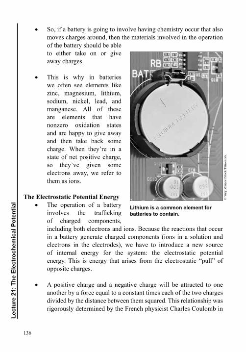
136

Lect

ure

21: T

he E

lect

roch

emic

al P

oten

tial

• So, if a battery is going to involve having chemistry occur that also moves charges around, then the materials involved in the operation of the battery should be able to either take on or give away charges.

• This is why in batteries we often see elements like zinc, magnesium, lithium, sodium, nickel, lead, and manganese. All of these are elements that have nonzero oxidation states and are happy to give away and then take back some charge. When they’re in a state of net positive charge, so they’ve given some electrons away, we refer to them as ions.

The Electrostatic Potential Energy• The operation of a battery

involves the trafficking of charged components, including both electrons and ions. Because the reactions that occur in a battery generate charged components (ions in a solution and electrons in the electrodes), we have to introduce a new source of internal energy for the system: the electrostatic potential energy. This is energy that arises from the electrostatic “pull” of opposite charges.

• A positive charge and a negative charge will be attracted to one another by a force equal to a constant times each of the two charges divided by the distance between them squared. This relationship was rigorously determined by the French physicist Charles Coulomb in

Lithium is a common element for batteries to contain.

© Y

ury

Min

aev/

iSto

ck/T

hink

stoc

k.

137

1785, and it is therefore known as Coulomb’s law, and the constant in the equation is known as Coulomb’s constant.

• We can compute work done from the Coulomb force. The displacement in this case is the change in the distance between the two charged species. You can think of the Coulomb force of repulsion between the two species as the two particles having energy stored in the electrostatic field, and you can think of this energy as being potentially available whenever it is needed. You can think of the potential energy for an electrostatic force as being defined as the capacity for doing work that arises from the position or configuration of the charges.

• Any collection of charges will have a potential energy associated with it. So, the general expression for the potential energy of a given charge (q) that comes near another fixed charge (Q) is equal to the following work expression: Velectrostatic = kqQ/r2, where k is Coulomb’s constant.

• The electrostatic potential energy per unit of charge is units of joules per coulomb, so we often divide the above expression by that test charge q to arrive at the following: Electrostatic potential per unit charge is equal to Coulomb’s constant (k) times the charge of the fixed particle Q divided by the distance it is from that particle (r): kQ/r.

• Because the charge of the test particle has been divided out, the electrostatic potential is a property that is related only to the electric field itself and not the test particle. For this version, we usually use the symbol Φ, and in this case, the work done to bring a particle with charge q to any point in space will equal the electrostatic potential Φ at that point times the charge q.

• The electrostatic potential is the key variable we need for our thermodynamics. And the thermodynamic work expression for a charged particle is equal to the charge of the particle times Φ, where Φ depends on the position of the particle.

138

Lect

ure

21: T

he E

lect

roch

emic

al P

oten

tial

The Electrochemical Potential• The electrochemical potential will become a new term in the

fundamental equation for the internal energy—a term that accounts for the new form of energy that arises due to the separation of charges in a system.

• For a closed system where only mechanical work is possible, the fundamental equation is written as dU = TdS − PdV, assuming a reversible process. However, there can be many other forms of work, and they simply get added to the right-hand side of this equation if they are present in the system.

• So, for the case of chemical work, we have an addition term—the sum over all chemical components in the system of the chemical potential of each component times the change in the total number of

moles of that component: 1

n

i ii

dNµ=∑ .

• For electrostatic work, we add another term to the right-hand side, namely a sum over each component of the electrostatic potential for that component times the change in the total charge of that component. This is the electrostatic work term, which can be incorporated into the same sum over the different components.

• The electrochemical potential is the combination of those two terms in the summation over the number of components: the chemical work and the electrostatic work. However, wouldn’t it be nice if we could rewrite this as a single potential? In fact, we can. To do so, all we need to do is rewrite that change in the total charge of a given component in the system as a change in the number of moles of that same component. This will bring us to our final definition of the electrochemical potential.

• To do this transformation, we introduce new terms. The total charge of a given component in the system is the valency (Z ) of that component times the charge of an electron times Avogadro’s number times the number of moles of that component.

139

• The valency is simply the number of electrons that the component typically gives up. For zinc, for example, this number is +2 because it likes to lose 2 electrons. For sodium, this number would be +1 because it likes to lose only a single electron.

• The number of electrons a given component likes to give up times the charge of an electron is equal to the charge each component (this could be an atom or a molecule) likes to give up. Avogadro’s number times the number of moles of that component is the total number of them. A mole of zinc atoms would be 6 × 1023 atoms. So, when we multiply this all together, it is exactly equal to the total charge that the given component has in the system.

• We now have a description of the electrostatic potential that depends on the change in the number of moles of a component. This allows us to group it together with the chemical potential term. And we can use Faraday’s constant (F ) instead of the charge of an electron times Avogadro’s number. Finally, we have the fundamental equation expression, which now has

dU = TdS − PdV + 1

n

i ii

dNµ=∑ .

• We write the electrochemical potential with the same symbol as the chemical potential (μ), but to signify that it’s been “electrified,” we add a small line on top of it (͞μ). And ͞μ is equal to μ plus the valency (Z ) times Faraday’s constant (F ) times the electrostatic potential Φ: ͞μ = μ + ZFΦ.

• The electrochemical potential contains the intrinsic chemical potential of each component plus the electrostatic potential acting on charged species. Just as the chemical potential of a species must be the same in all phases at equilibrium, the electrochemical potential of charged components must be the same in all phases to reach electrochemical equilibrium.

140

Lect

ure

21: T

he E

lect

roch

emic

al P

oten

tial

• A battery operates by extracting electrical work from a chemical reaction. And just as with chemical reactions, electrochemical reactions can be analyzed using the Gibbs free energy and the chemical potential in order to determine the equilibrium state at constant temperature and pressure. The Nernst equation relates the electrostatic potential energy change to the change in free energy of the overall reaction for the system divided by 2 times Faraday’s constant.



1. Where is the energy in a potato battery coming from?

2. How long will this battery last?

Suggested Reading


141

Chemical Reactions—Getting to EquilibriumLecture 22

In this lecture, you will learn about chemical reactions and how the concepts of thermodynamics can be used to tell us when a reaction will occur and when it will not. Chemical reactions are fundamentally part

of everything we do. In many processes, there is work being done, and it is a direct result of substances changing their nature. This is called chemical work, and it is based on a process wherein the number of moles of a component in the system changes. That chemical potential can be considered the thermodynamic force in a chemical reaction, and the change in number of moles is the thermodynamic displacement.

Chemical Reactions• Chemical reactions happen when, through some process, a set of

one or more chemical species become a set of one or more different chemical species that were not in the original state.

• Chemical reactions come in a variety of forms, including the following.o Decomposition: A single chemical species becomes two or

more species upon the reaction occurring.

o Synthesis: Two or more chemical species become a single species upon the reaction occurring.

o Displacement: The same number of chemical species is found before and after reaction, but the atomic species in the chemicals switch.

• Formally, we say that chemical reactions can be either exothermic or endothermic. In general, an endothermic reaction is one in which energy input is required for the reaction to occur, while an exothermic reaction is one that releases heat energy upon reacting.

142

Lect

ure

22: C

hem

ical

Rea

ctio

ns—

Get

ting

to E

quili

briu

m

• Endothermic and exothermic refer to the process of the reaction itself; they do not refer to any energy required to overcome a barrier to “get it going.”

• A few examples of endothermic reactions are melting an ice cube or evaporating water, baking bread or cooking anything, melting a solid, the way in which a chemical ice pack (such as one in a first aid kit) works, and the photosynthesis part of plants growing.

• A few examples of exothermic reactions are burning a candle, making an ice cube from water, rusting iron, the way in which a chemical hot pack works, burning gas on your stove, and nuclear fission.

• In terms of thermodynamics, the most important topic of interest is to find an answer to the following question: Which direction will a chemical reaction occur? This, of course, depends on the current equilibrium conditions of the system.

Burning a candle is an example of an exothermic reaction.

© fa

thad

am/iS

tock

/Thi

nkst

ock.

143

• For standard chemical reactions in a lab, the control variables are typically temperature and pressure. When we have those conditions of constant temperature and pressure, there is a particular thermodynamic variable, a potential energy variable, that is extremely useful, and it will be the one we use to analyze reactions—the Gibbs free energy.

• As a reminder, the Gibbs free energy is equal to the internal energy minus temperature times entropy plus pressure times volume: G = U − TS + PV. (This can also be written as G = H + PV to incorporate enthalpy).

• By considering the first law and our definition of entropy in a reversible process, the differential form of the Gibbs free energy

can be written as follows: dG = −SdT + VdP + 1

n

i ii

dNµ=∑ .

• This type of equation is called a fundamental equation, because such an equation completely specifies all changes that can occur in the given thermodynamic system. Fundamental equations form the basis for applying the second law of thermodynamics to identify the equilibrium state of a given system.

• If a chemical reaction occurs at constant temperature and pressure, the change in Gibbs free energy in a chemical reaction will tell us whether a reaction will go in the forward or in the reverse direction.

• If the change in G for a given reaction (∆Grxn) is less than zero, then the forward reaction is favored. If it’s equal to zero, then the reaction is in equilibrium, and if it’s greater than zero, then the reverse reaction is favored. This makes sense when considering the second law of thermodynamics, which states that the entropy of the universe for any spontaneous process must increase, and the definition for the change in the Gibb’s free energy.

144

Lect

ure

22: C

hem

ical

Rea

ctio

ns—

Get

ting

to E

quili

briu

m

• From this equation for the change in the Gibbs free energy, for a system at constant temperature and pressure, dG is equal to a sum over all the components in the system of the chemical potential of that component times its change in number of moles.

Balancing Chemical Reactions• The chemical potential dictates mass flow. It is what we consider to

understand how molecules in a reaction are driven from one phase into another in closed systems or how the addition or subtraction of molecules occurs in open systems. We add up the chemical potentials of each side of a reaction, and the heavier side—that is, the side with the largest chemical potential—is the side that we can consider to be the reactants.

• To find the equilibrium condition for any given reaction, we find the point at which the change in the Gibbs free energy (dG) is zero. For a given reaction, this will equal the sum over those chemical potentials times number of moles, where we use a positive sign for the species on the right and a negative sign for the ones on the left. This gives us the net change in G for that possible process.

• However, we cannot simply create something out of nothing, so we must make sure that the reaction is balanced. In thermodynamics, while chemical species may change from one form to another in a given reaction, the total number of atoms is conserved. So, the two sides of the reaction have to be balanced.

• For example, we can’t write H2O → H2 + O2, even though we know that the two diatomic molecules are what form. Instead, to find the balance, we write this as 2H2O → 2H2 + O2 so that the number of hydrogen and oxygen molecules, although they’ve taken on new meaning by decomposing, is fully conserved.

• Those coefficients that end up balancing the reaction—and we like to use integers instead of fractions—are called the stoichiometric coefficients of the reaction. These numbers are very important because if we “feed” a reaction with a certain number of moles

145

of reactant, then the stoichiometric coefficient tells us something about how many moles of reactant we will get. In fact, it tells us how many moles of what needs to be mixed with how many moles of something else in the first place.

The Haber Reaction• The following reaction is arguably the single most important

reaction developed in human history: N2 + 3H2 → 2NH3. Notice that this is balanced and that we have produced ammonia from nitrogen and hydrogen.

• This reaction is important because it was the first time humans could make nitrogen how plants like it, and that ability led to a new way of growing food, leading to the industrial revolution of food. This process takes nitrogen from an unusable form and makes it usable in the form of ammonia. This process is called “fixing” the nitrogen, which just means converting it into some biofriendly form.

• There are two important things we do to quantify this aspect of reactions. First, we want to know the change in free energy per mole of reaction. Second, we only really want to know this for the amount of the reaction that has occurred to completion—or, as it is often called, the extent of the reaction.

• This extent concept can be understood as considering the reaction occurring in terms of the change in number of moles of a given species divided by the stoichiometric coefficient for that species. The change in free energy for the reaction is then divided by this “scaled” change in number of moles, which leads to what we want—namely, the change in the Gibbs free energy per mole of reaction that actually occurs.

• A thermodynamic analysis of reactions only tells us about the equilibrium case—that is, eventually what the reaction will do given enough time. The ideas of metastability, of barriers to reactions occurring, and of the timescale over which a reaction occurs do not come from our thermodynamic analysis.

146

Lect

ure

22: C

hem

ical

Rea

ctio

ns—

Get

ting

to E

quili

briu

m

• For the Haber reaction, the key discovery was not that the reaction occurs but, rather, how to make it occur much more efficiently by introducing catalysts that create intermediate processes and by varying the pressure to allow for large scales, high output, and low costs.

• The simple question of whether a reaction will occur or not, given that the system can find a way to its happy place, is crucial because it forms the basis of even how to think about ultimately what can be made from what.

Callen, Thermodynamics and an Introduction to Thermostatistics, Chap. 8 and 13.

DeHoff, Thermodynamics in Materials Science, Chaps. 8 and 11.


1. What are the different types of reactions that can occur?

2. Can thermodynamics tell us anything about how fast a reaction is expected to happen?

3. Why were so many bubbles produced in the demo?

4. Estimate the change in entropy of the universe after the reaction from the demo.

Suggested Reading


147

The Chemical Reaction QuotientLecture 23

In this lecture, you will learn about a crucial concept in the application of thermodynamics to reactions—namely, the activity coefficient and how it relates to concentration and the chemical driving force during a

reaction. This, in turn, will lead you to a way to compute this driving force at any concentration and to an equation to find the equilibrium of a reaction. This is of fundamental importance when the ability of a reaction to occur depends on the concentrations of the reactants and products, which are changing during the reaction.

The Activity Coefficient• What we want to know, and what thermodynamics can tell

us, is which way reactions will go when they occur. However, thermodynamics does not tell us whether they will go or not; it only tells us if the energy gradient favors the reaction.

• There often are kinetic barriers to the reaction occurring. We can figure out if a reaction will occur by adding up the values of the standard-state molar free energies for each compound, and from those, we can calculate ∆G of the reaction.

• Chemical reactions of any kind can proceed initially in one direction or the other, dictated by the difference in free energies between the reactants and products. Either way it goes, the reaction can then stop for two reasons: One of the reactants is simply used up, or the reaction reaches an equilibrium state—with all products and reactants still present but now in some sort of new balanced condition.

• The way we describe the second case, where reactant and product concentrations in solution are changing, is by considering the change in the chemical potential as a function of concentration for each component involved in the reaction.

148

Lect

ure

23: T

he C

hem

ical

Rea

ctio

n Q

uotie

nt

• There is always additional entropy caused by mixing, and it only depends on the concentrations of the mixtures. As the mole fraction of one of the components varies, the molar entropy of mixing increases as two components are mixed and reaches a maximum for a 50-50 mixture.

• From this expression for the entropy of mixing, we can also write down expressions for the free-energy change upon mixing. We can write the chemical potential of either one of the species in the mixture as having changed due to the concentration of that component changing.

• In the example of two components A and B mixing, the chemical potential of A is equal to the standard-state chemical potential of A (μo

A) plus the gas constant (R) times the temperature (T ) times the natural log of the mole fraction of component A (lnXA): μA = μo

A + RT lnXA.

• This is a powerful equation that tells us how the Gibbs free energy varies with changes in concentration of something in solution. However, this form of the equation only applies to ideal solutions, meaning that we have ignored interactions, just like in the ideal gas law. So, the equation only considers changes in the free energy—or chemical potential if we take the molar free energy—due to the entropy of mixing.

• But most reactions are not ideal because interactions between components can be very different from the interactions of one component with itself. For the components A and B, this would mean that A and B have a very different bonding character than either A with A or B with B. This kind of effect is not taken into account in the ideal-solution model.

• So, we need to expand the range of applicability of this relationship. However, this form of the equation, where we take the standard-state chemical potential and add a single term that goes as the

149

logarithm of something, is a very convenient mathematical form, so we’d really like to retain it. We do this by defining something called the activity (a).

• The chemical potential for a given component—for example, component i—at any concentration is equal to the chemical potential for that component at standard-state conditions (in other words, when it is in its pure form and not reacting) plus RT times the natural logarithm of the activity of that component: μi = μo

i + RT lnai.

• Quite simply, we have replaced the mole fraction with the variable ai. But it is a very powerful switch, because now we can essentially include any changes that happen to the chemical potential of the reacting species during the reaction. At the same time, we retain the same mathematical form—namely, a natural logarithm.

• It’s nice to write the activity in terms of the activity coefficient, for which we use the symbol gamma (γ), times the mole fraction of that component: μi = μo

i + RT ln(γ)Xi. By writing it this way, we can see how far away from the ideal-solution model the system is.

• For example, if γ for a component is equal to 1, then the activity of that component becomes the mole fraction of the component. We get back the same equation for the chemical potential that we had when we ignored interactions and just had the ideal-solution model.

• The ideal-solution model means that the chemical potential will change upon mixing things together, but only because the entropy of the mixture increases. The activity, which includes the interactions, can tell us how important the interactions were in the first place. Interactions of components can lead to a huge difference in the effects of mixing, even fully reversing the qualitative effects of mixing.

150

Lect

ure

23: T

he C

hem

ical

Rea

ctio

n Q

uotie

nt

Raoult’s Law and Henry’s Law• The deviation of the activity coefficient from 1 is a measure of

how far away from ideal the system is. And in so many cases for reactions, the activity coefficient can vary quite a bit as a function of the mole fraction of each species in the solution. The factor by which the activity coefficient deviates from 1 has an enormous impact on the chemical behavior of the system, which is driven by the chemical potential.

• As the concentration of the mixture changes, the activity coefficient also changes. Once the activity coefficient converges to around 1, the solution behaves pretty much like an ideal solution. This limit, where the solution starts to behave like an ideal one because the concentration is approaching 1, is called Raoultian behavior. Raoultian behavior simply means ideal behavior, so we’re back to the chemical potential of mixing depending on the natural log of just the molar concentration.

• François-Marie Raoult was a French physicist who was experimenting with vapor pressures around 1882. He noticed that if he had a solution of two liquids—for example, A and B—then as long as no other gases were present, the total vapor pressure above the solution was equal to the weighted sum of the “pure” vapor pressures of the two components.

• He found that the total vapor pressure (P) is equal to the mole fraction XA times the partial vapor pressure PA plus XB times PB: P = XA PA + XB PB. Although we’re talking about pressures, this is equivalent to the same ideal-solution-model behavior we found for the free energy and chemical potential.

• For low concentrations, just as with the high-concentration regime, we call the behavior of the mixture Henrian. William Henry formulated Henry’s law in 1803, and like Raoult, he was also playing around with liquids and gases and measuring pressures.

151

• Henry’s law states that at a constant temperature, the amount of gas that dissolves in a liquid is proportional to the partial pressure of that gas in equilibrium with the liquid. For a dilute solution, Henry’s law tells us that the pressure goes as a constant (called Henry’s constant, kH) times the molar concentration of the solute (C ): P = kHC.

• It is interesting to compare this to Raoult’s law, which states that the pressure goes as the partial pressure of that component in its pure state times its mole fraction, valid for the other extreme—at high concentration.

• Both of these laws appear to give something similar: a dependence of a constant times a mole fraction. This is actually true if the two components being mixed have a similar bonding behavior with each other as they do with themselves. But that’s just for the ideal-solution case.

• If interactions are strong and different between the two components, then in the case of Henrian behavior, we are looking at a regime where these differences are in a sense maximized, because each solute is surrounded primarily by only solvent, as opposed to other solute molecules.

The Equilibrium Constant• The change in the chemical potential in a reaction is equal to

the difference in the standard-state chemical potentials plus RT times the natural log of what is called the reaction quotient (Q): ∆G = ∆Go + RT lnQ. This reaction quotient is the ratio of the activities of the products multiplied together, divided by the activities of the reactants multiplied together.

Physician and chemist William Henry (1775–1836) proposed what is now known as Henry’s law.

© B

y co

urte

sy o

f the

trus

tees

of t

he B

ritis

h M

useu

m/

Wik

imed

ia C

omm

ons/

Publ

ic D

omai

n.

152

Lect

ure

23: T

he C

hem

ical

Rea

ctio

n Q

uotie

nt

• The activities in the Q change during the reaction as the system strives to reach equilibrium, and these activities are highly dependent on concentration. The concentrations of these components are changing as they react, so the activities will change as well.

• This reaction quotient allows us to keep being able to calculate the chemical driving force for the reaction at any point, as long as we also know what the activities are for the reactants and products.

• At the special point at which this driving force, this change in chemical potential due to a reaction occurring, is zero, there is no longer a way for the system to lower its free energy, so it is in equilibrium.

• We can find this point simply by plugging in zero for the change in chemical potential. We find that the equilibrium point for the reaction is determined when the RT natural log term is equal to those differences in standard-state chemical potentials.

• This point, where we have equilibrium, is so important that we call the reaction quotient at that point the equilibrium constant. It’s still just the same reaction quotient, but it only refers to the equilibrium point in the reaction, so many textbooks give that its own variable (often K ).

• Among those who do a lot of chemistry, this equation for the equilibrium of a reaction has been considered the most useful in thermodynamics. Most important is the fact that the activity product ratio that makes up the equilibrium constant is independent of variations in the system composition. The equilibrium constant K is controlled completely by the difference in standard chemical potentials.

153

• This means that it is only a function of the temperature and pressure. And for any given temperature and pressure, it’s a constant. As soon as the substances reacting are chosen, then the value for the equilibrium constant is fixed. It is the activity product ratio that would be observed if the system reaches equilibrium.

• The equilibrium constant is a very useful piece of information to have about a reaction. If K is very large, it shows that a reaction will tend to go “to completion”—that is, mostly products will be present at equilibrium—and if K is small, it shows that the reaction hardly goes at all before enough products are formed to stop it.

• The equilibrium constant will not tell you whether reactants will actually react or at what rate; instead, it indicates the activity product ratio at equilibrium, not whether equilibrium is easily achievable. The reaction continues until the ratios of the activities of the products and reactants equal this equilibrium constant.




1. What is the molar Gibbs free energy of formation for an element?

2. What is the difference between the equilibrium constant and the reaction quotient?

3. What is the difference between an exothermic and an endothermic reaction?

Suggested Reading


154

Lect

ure

24: T

he G

reat

est P

roce

sses

in th

e W

orld

The Greatest Processes in the WorldLecture 24

The laws of thermodynamics, and the variables they govern, ultimately describe how energy moves. They describe why energy transforms from one form into another and how matter is affected during these

transformations. The technologies we still need to invent in order to address the world’s future energy—and water—needs will rely on the design of new materials, and that can only be done with an intimate knowledge of thermodynamics. By learning thermodynamics, we learn how to understand, describe, predict, and design the greatest processes in the world.

The Value of Energy• Fossil fuels have been able to completely change the world in

essentially every way imaginable in what is by any measure quite a short time period. And scientists and engineers have been at the forefront of this revolution: whether by helping to design new ways to find and extract the energy from the ground, or new ways to use this energy in our factories, in our farms, in our transportation, and in our homes.

• The ability to burn carbon-based materials is what powers our industry, growth, and comfort. But all of these massive amounts of ultra-cheap energy have also led our world to quite a strained position. Concerns about sustainability, climate, and national security are requiring that we reexamine our reliance on carbon burning.

• Among the many thought-provoking questions these topics have inspired, one entirely practical question is critical: Is the burning of carbonaceous materials the only way in which our planet can be tapped for energy?

155

• Currently, there is enough ancient sunlight trapped in carbonaceous forms—whether from conventional or unconventional reservoirs—to last at least another generation, maybe more. But as our 200-year blip of seemingly limitless fossil fuel energy begins to decline, we will have to rely on alternative and sustainable energy resources. Fossil fuels are finite; eventually, and not too far from now, they will run out.

• The energy we get from fossil fuels is so dense and such a precious resource that it is a daunting task to even think about how we might someday be able to fully replace them. Unlike many other revolutions that have occurred, the revolution that must occur in energy and water over the next century will almost entirely center on our ability to carefully design and manufacture completely new materials.

• Ironically, it is precisely because of the foundational science and engineering discoveries enabled by thermodynamics that we have arrived at this global tipping point. Now that we are where we are in human civilization, there is no starting over. We need to look to the future, and we need to use the science and technology that we have learned over the past centuries to place humanity in a more sustainable position with respect to the planet.

• So, instead of asking what would happen if we had to begin again, we need to ask the following: What happens now that we cannot begin again? Thermodynamics is the answer to this critical question. Scientists and engineers have used subjects like thermodynamics to harness energy to build our modern society, and they are also the ones who must create a new way to get that energy.

• The work to invent and develop and optimize alternatives to fossil fuels must be done now, because it is long-term work that might take decades. Scientific breakthroughs cannot be predicted, but it is easy to predict that if we don’t put any people and resources onto a problem, then no breakthroughs can occur. We need to work now on this problem so that we are ready for it later.

156

Lect

ure

24: T

he G

reat

est P

roce

sses

in th

e W

orld

Solar Thermal Fuels• An example of a new type of fuel that is being developed is called

a solar thermal fuel, which is a material that absorbs sunlight really well, and when it’s exposed to the Sun, it undergoes a transformation at the molecular level. As light shines on the molecule, it changes its shape. In its new, twisted shape, the molecule stores energy—a kind of energy that can be released later, whenever you need it, in the form of heat. Once the energy is released, the fuel is ready to be recharged by the Sun.

• Temperature is related to vibrational motion, and that the heat capacity of a material depends on how many internal degrees of freedom are available to store the energy. This case has a special atomic arrangement where it can store even more internal energy, but it’s not taking in thermal energy to get there—instead, it’s converting sunlight energy into this specially strained internal energy state.

• When the molecule is triggered, it goes back to its original position, and as it does, the motion of the molecule is so intense that it’s like a little tiny explosion. And because the motion of atoms is related to temperature, the temperature of the molecule goes way up, and thermal energy is released.

• It still all comes down to the thermodynamics of the energy pathways. In this case, we have sunlight to chemical energy to thermal energy. One way to think of a solar thermal fuel is that it’s like a rechargeable heat battery. It can be charged over and over again by the Sun and deliver heat on demand when needed.

• This type of fuel could completely change the way we make and use energy. First, unlike fossil fuels, it’s a material that operates in a manner that leads to no by-products. The fuel does not combust but, rather, simply cycles back and forth between the charged and the uncharged states.

157

• Second, it’s chargeable by the Sun, so it is based on a resource that is effectively infinite. Third, it represents the only way to use the Sun’s energy in the form of heat that is distributable and transportable. That’s because other solar thermal technologies do not store the energy indefinitely until it is purposefully released but, rather, simply get hot and then immediately begin losing that stored heat.

• Because of their potential advantages, it’s perhaps not surprising that solar thermal fuels are not new. They were heavily explored in the 1970s, although they were widely abandoned by the mid-1980s because the materials under consideration back then simply could not withstand the cycling. They would degrade a little bit each time they charged. After a mere 10 or 20 cycles, the amount of useful fuel left was miniscule.

• By optimizing the thermodynamic free energy of this system, we have invented an entirely new platform for making solar thermal fuels, one that leads to materials that can be recharged over and over again with absolutely no degradation for tens of thousands of cycles and that have energy densities even higher than the best-performing batteries on the market today. This represents the first sunlight rechargeable thermal fuel that provides safe, recyclable, high-density, transportable, and distributable heat on demand. And it’s entirely possible because of thermodynamics.

• One example of how we’re using solar thermal fuel already is in solar cooking. Solar cookers exist, but a key limitation is that until now, you could only cook with them when the Sun was shining. With solar thermal fuels, we’ve created a new cooker. You can charge it up during the day by leaving it out in the Sun, and then when you want to cook, you can simply flow the charged-up fuel the other way and trigger it to release the stored heat.

158

Lect

ure

24: T

he G

reat

est P

roce

sses

in th

e W

orld

Water and Energy• Water and energy are intimately related to one another. That’s

because producing and transporting freshwater takes massive amounts of energy. And it’s not just about energy required to get water; it’s also about the water required to get energy. The energy security of the United States remains precariously reliant on large volumes of freshwater for cooling.

• But the biggest challenge with water is in the availability of it. Even though 70 percent of the planet is covered with water, less than 3 percent of that is freshwater, most of which is locked up as ice in polar caps and glaciers. This leaves less than 1 percent of all of Earth’s water as drinkable.

• One way to solve this challenge would be to invent a way to take the salt out of ocean water in order to make it drinkable. This process is called desalination, and there are many ways to do it, but the problem is that none of these ways is cheap enough to become a global solution to freshwater, at least not currently.

most of the less than 3 percent of water that is freshwater is locked up as ice in polar caps and glaciers, meaning that it is undrinkable.

© T

im D

e B

oeck

/iSto

ck/T

hink

stoc

k.

159

• The most efficient technique we have today is called reverse osmosis, which is based on massive pumps to push saltwater across specialized membranes that, at high enough pressures, will allow the water to pass but not the salt.

• To desalinate water, we need to overcome the entropy of mixing, which is quite powerful. We have to get to pretty high pressures to force water to be unmixed and move to lower entropy states. The pressure that drives the water to higher entropy is called the osmotic pressure. The cost of the energy required to overcome the osmotic pressure is enormous.

• Most of the ancillary processes involved in desalination have already been intensively optimized over the past several decades, but the membrane itself—the key material involved in the process—has been based on the same technology for the past 40 years. If we want to turn desalination into an environmentally benign and economically affordable solution for the global water supply, we need to completely rethink the membrane.

• In the new age of materials design and with a solid understanding of thermodynamics, we have used thermodynamics to design the ultimate membrane for water desalination. At only a single atom thick, it is the thinnest membrane that one could ever make. The material that allows us to make such a membrane is called graphene, and it’s a sheet of carbon atoms that looks like a honeycomb lattice.

• However, we cannot desalinate water with this single-atom-thick material in its natural form. For that, we need to make holes in the graphene that are just the right size. They need to be big enough to let water pass through but small enough so they block the salt from going through.

• This is where thermodynamics enters the picture: The key to understanding and therefore designing just the right pores lies in controlling the entropy of the water molecules as they pass through the membrane.

160

Lect

ure

24: T

he G

reat

est P

roce

sses

in th

e W

orld

• By tailoring the pore in just the right way, we are able to maximize the entropy of the water while keeping the pore small enough to completely reject the salt. The result is a completely new membrane for desalinating water.


Callister and Rethwisch, Materials Science and Engineering, Chaps. 1 and 22.


1. Name your favorite thermodynamic processes and variables, and think about how you could use these to process a material in a particular manner.

2. At its core, what is thermodynamics about?

3. How does thermodynamics enter into your daily life?

Suggested Reading


161

Bibliography

Anderson, Greg. Thermodynamics of Natural Systems. 2nd ed. Cambridge: Cambridge University Press, 2009.

Callen, Herbert B. Thermodynamics and an Introduction to Thermostatistics. 2nd ed. Hoboken, NJ: Wiley, 1985.

Callister, William D., and David G. Rethwisch. Materials Science and Engineering: An Introduction. 8th ed. Hoboken, NJ: Wiley, 2009.

DeHoff, Robert. Thermodynamics in Materials Science. 2nd ed. Boca Raton, FL: CRC Press, 2006.

Halliday, David, Robert Resnick, and Jearl Walker. Fundamentals of Physics. 9th ed. Hoboken, NJ: Wiley, 2011.

Lambert, Frank L. “Shuffled Cards, Messy Desks, and Disorderly Dorm Rooms—Examples of Entropy Increase? Nonsense!” Journal of Chemical Education 76, no. 10 (1999): 1385.

Moran, Michael J., Howard N. Shapiro, Daisie D. Boettner, and Margaret B. Bailey. Fundamentals of Engineering Thermodynamics. 7th ed. Hoboken, NJ: Wiley, 2010.

Porter, David A., and Kenneth E. Easterling. Phase Transformations in Metals and Alloys. 2nd ed. Boca Raton, FL: CRC Press, 1992.

Serway, Raymond A., and John W. Jewett. Physics for Scientists and Engineers. 9th ed. Chaps. 19–22. Independence, KY: Cengage Learning, 2013.

thermodynamics: four laws that move the universe · pdf filephysics science & mathematics...

Documents