Thermodynamics based stability analysis and its use for

nonlinear stabilization of the CSTR.

N.H. Hoang, Francoise Couenne, Christian Jallut, Yann Le Gorrec

To cite this version:

N.H. Hoang, Francoise Couenne, Christian Jallut, Yann Le Gorrec. Thermodynamics basedstability analysis and its use for nonlinear stabilization of the CSTR.. Computers & ChemicalEngineering, 2013, 58, pp.156-177. <hal-00876537>

HAL Id: hal-00876537

https://hal.archives-ouvertes.fr/hal-00876537

Submitted on 24 Oct 2013

HAL is a multi-disciplinary open accessarchive for the deposit and dissemination of sci-entific research documents, whether they are pub-lished or not. The documents may come fromteaching and research institutions in France orabroad, or from public or private research centers.

L’archive ouverte pluridisciplinaire HAL, estdestinee au depot et a la diffusion de documentsscientifiques de niveau recherche, publies ou non,emanant des etablissements d’enseignement et derecherche francais ou etrangers, des laboratoirespublics ou prives.

1

Thermodynamics based stability analysis and its use for

nonlinear stabilization of the CSTR

N. H. Hoang

Faculty of Chemical Engineering, University of Technology, Vietnam National University - Ho Chi Minh City

268 Ly thuong Kiet Str., Dist. 10, HCM City, Vietnam

ha.hoang@hcmut.edu.vn

F. Couenne, C. Jallut* Université de Lyon, F-69622, Lyon, France; Université Lyon 1, Villeurbanne, CNRS UMR 5007, LAGEP

couenne, jallut@lagep.univ-lyon1.fr

Y. Le Gorrec ENSMM Besançon, FEMTO-ST/AS2M, France

Yann.Le.Gorrec@ens2m.fr

*: author to whom correspondence should be addressed

Abstract: We show how the availability function as defined from the entropy function

concavity can be used for the stability analysis and derivation of control strategies for non-

isothermal Continuous Stirred Tank Reactors (CSTRs). We first propose an overview of the

required thermodynamic concepts. Then, we show how the availability function restricted to

the thermal domain can be used as a Lyapunov function. The derivation of the control law and

the way the strict entropy concavity is insured are discussed. Numerical simulations illustrate

the application of the theory to the open loop stability analysis and the closed loop control of

liquid-phase non-isothermal CSTRs. The proposed approach is compared with the classical

proportional control strategy. Two chemical reactions are studied: the acid-catalyzed

hydration of 2-3-epoxy-1-propanol to glycerol subject to steady state multiplicity and the

production of cyclopentenol from cyclopentadiene by acid-catalyzed electrophilic addition of

water in dilute solution exhibiting a non-minimum phase behavior.

Keywords: Availability; Entropy; CSTR, Stability; Nonlinear control; Lyapunov function.

1. Introduction

*Manuscript (for review)Click here to view linked References

2

The aim of this paper is twofold: to provide an overview of the existing thermodynamic

concepts required for dynamic stability analysis of irreversible physicochemical systems and

to describe, in the case of the single-phase CSTR, how to derive a stabilizing Lyapunov based

control law from the so called thermodynamic availability function. This thermodynamically

driven systematic approach is of interest as such processes are highly nonlinear mainly due to

chemical reaction kinetics while the coupling between energy and material balances can lead

to multiple steady states (Perlmutter, 1972) or non-minimum phase behavior (Engell and

Klatt, 1993; Van de Vusse, 1964).

The stability analysis and the design of control laws of CSTRs are widely studied in literature.

Usually, the stability analysis is based on mathematical tools such as linearization methods

(see for example Aris and Amundson, 1958; Uppal et al., 1974) or direct Lyapunov methods

(see for example Perlmutter, 1972; Warden et al., 1964). Direct Lyapunov methods are based

on the definition of the so-called ―energy‖ storage function that is subject to dissipation

(Ramírez et al., 2009) and is very often quadratic. In general even for open thermodynamic

systems, this storage function has not the dimension of energy. Indeed in this case, the stored

energy is the internal energy and, from the first law of thermodynamics, no dissipation occurs

since energy is a conserved quantity.

As far as control design is concerned, numerous contributions have been published with

respect to applications and to theoretical developments. An overview of classical methods for

chemical processes control is presented in (Bequette, 1991). In many applications, the

objective is only to regulate the temperature of the chemical reactor. This problem has been

successfully solved by differential geometry approaches such as output feedback linearization

3

(Viel et al., 1997) for control under constraints, by nonlinear PI control (Alvarez-Ramirez and

Puebla, 2001) and direct Lyapunov-based methods for the design of nonlinear output

feedback control laws (Antonelli and Astolfi, 2003).

As far as thermodynamic methods are concerned, since the pioneering works of Glansdorff

and Prigogine (Glansdorff and Prigogine, 1971), it is well established that the irreversible

thermodynamics theory can be applied to the stability analysis of physicochemical systems. A

thermodynamics based Lyapunov function related to the irreversible entropy production has

thus been used for local stability analysis of a CSTR (Dammers, 1974 ; Tarbell, 1977). The

question of control design can also be addressed within this framework. The idea of control

by energy/power shaping has been recently developed (Favache and Dochain, 2009, 2010 ;

Ramírez et al., 2009; Battle et al., 2010; Alvarez et al., 2011). A physical interpretation of

slow and fast modes of process dynamics based on linearized models has been given

(Georgakis, 1986). Simple extensive variables are then used for the control design by

regulating the fast mode. Georgakis stability analysis method has been extended to a reaction

leading to a possible equilibrium with less restrictive assumptions (Favache and Dochain,

2009). The authors proposed different thermodynamic Lyapunov function candidates for a

wide range of operating conditions. Finally, the concept of availability as it has been proposed

within the framework of passivity theory for processes (Alonso and Ydstie, 1996; Ydstie and

Alonso, 1997; Farschman et al., 1998; Ruszkowski et al., 2005) is inspired from the concepts

developed by the Brussels School of Thermodynamics (Glansdorff and Prigogine, 1971). As a

matter of fact, in order to study the stability of physicochemical systems, Prigogine and co-

workers have used the local curvature of the entropy function. The concept of availability is

the nonlinear extension of this curvature as it will be shown in the first section of this paper.

4

This concept is very general since it also allows dealing with the control of infinite

dimensional processes (Alonso et al., 2000; Alonso and Ydstie, 2001; Alonso et al., 2002).

Nevertheless, in all these studies, control design is achieved by using passive techniques,

especially for the distributed or network systems, with some restrictions on the chemical

reaction kinetics and/or operating conditions, for instance isothermal/adiabatic conditions or

close to the thermodynamic equilibrium state (Farschman et al., 1998; Alonso and Ydstie,

2001; Ruszkowski et al., 2005). The strategy developed in this paper is quite different as a

nonlinear state feedback is used to shape a desired closed loop Lyapunov function. This

closed loop Lyapunov function is directly derived from the aforementioned availability

function and can be applied to one or multiple reactions system operating far from

equilibrium (Hoang et al., 2012) as well as to intensified continuous and batch slurry reactors

(Bahroun et al., 2010, 2013) as soon as the system states are unique at a given temperature.

Such a nonlinear feedback allows compensating the main non-linearity that is due to the

chemical reaction rate (Antonelli and Astolfi, 2003).

The paper is organized as follows. The availability function as defined by Ydstie and co

workers (Alonso and Ydstie 1996; Ydstie and Alonso, 1997; Farschman et al., 1998; Alonso

et al., 2000; Alonso and Ydstie, 2001; Alonso et al., 2002; Ruszkowski et al., 2005) is

introduced within the general framework of the second law of Thermodynamics. The way the

time derivative of this availability function is derived for the CSTR is exposed. Provided that

a condition of strict concavity for the entropy function can be satisfied, this availability

function will be used as a Lyapunov function for the open loop dynamic stability analysis and

for the design of a stabilizing control law for the jacketed single-phase non-isothermal CSTR.

This control strategy, applicable to a large class of chemical reactors is illustrated by two

examples of particular interest. The first one is an example of single reaction system subject

5

to steady-state multiplicity, the acid-catalyzed hydration of the 2-3-epoxy-1-propanol to

glycerol and the second one is an example of multiple reactions system that exhibits a non-

minimum phase behavior, the production of cyclopentenol from cyclopentadiene by acid-

catalyzed electrophilic addition of water in dilute solution. These chemical processes have

been widely studied in the literature (Heemskerk et al., 1980; Rehmus et al., 1983;

Vleeschhouwer et al., 1988; Vleeschhouwer and Fortuin, 1990) and (Engell and Klatt, 1993;

Niemiec and Kravaris, 2003; Antonelli and Astolfi, 2003; Guay et al., 2005; Chen and Peng,

2006) respectively and they exhibit some difficulties and challenges for control design and

stabilization problem. We have shown (Hoang et al., 2012) that physically admissible control

laws are obtained by using what we call the thermal part of the availability function and the

jacket temperature as the only manipulated variable. This thermal part of the availability is

obtained as soon as the availability of the bulk is separated into the sum of two terms. The

designed control law leads to closed loop global stabilization around a desired reference state.

Throughout the paper, the numerical simulations illustrate these developments via the two

above-mentioned examples. Finally, the designed control is compared to classical

proportional feedback with respect to closed loop performances and thermodynamic

properties.

2. Applications of the second law of Thermodynamics: a brief

overview of some fundamental concepts

The applications of the second law of Thermodynamics under consideration are based on the

concepts of availability, exergy or available work. On the one hand, these concepts have been

used for thermodynamic efficiency analysis of processes (Bejan, 2006). On the second hand,

equilibrium stability studies have been performed on this basis (Kondepudi and Prigogine,

6

1998). In this section, we give a brief overview of these concepts and the way they have lead

to dynamic stability studies.

2.1. Available work and exergy

It has been pointed out by Kestin (1980) that concepts of availability, available work or

exergy of a system are very similar. The aim of these concepts is to account for the capacity

of a system to exchange power and then to provide a method for comparing different systems

from this thermodynamic efficiency point of view. These concepts, that have been derived

mainly in the case of non-reacting systems, are firstly based on the definition of a passive

environment that is in contact with the system under consideration and that is characterized by

a constant pressure

P0 , a constant temperature

T0 and constant components i chemical

potentials

i0 (Sussman, 1980). Secondly, the system that has to be described is assumed to

exchange material with other systems k according to the molar flow rate of component i,

Fik,

as well as with the passive environment according to the molar flow rate of component i,

Fi0

.

Heat flows

0 and

m are also supposed to be exchanged by the system respectively with the

passive environment and with other heat sources at

Tm . The total power that is exchanged by

the system is divided into

P and

P0

dV

dt, the latter being due to mechanical expansion of the

system against the passive environment. In order to derive the power that the system is able to

exchange, we consider the material, energy and entropy balances, assuming that kinetic and

potential energies can be neglected:

7

dN i

dt Fik

k

Fi0 (a)

dU

dt0 m

m

P P0

dV

dt Fikhik

i,k

Fi0hi0 (b)i

dS

dt0

T0

m

Tmm

Fiksik

i,k

Fi0si0 (c)i

0 (d)

(1)

U, S and Ni are respectively the internal energy, the entropy of the system and the number of

mole of component i.

is the entropy production per time unit due to irreversible processes

that is nonnegative according to the second law of Thermodynamics.

hik and

sik are

respectively the partial molar enthalpy and entropy of the component i in the flow k. By

eliminating

0 that is coupling the energy and entropy balances equations (1b) and (1c) with

respect to the passive environment, one finds from equations (1a) to (1d):

d U P0V T

0S

i0N

i

i

dt

m1

T0

Tm

m

P Fik

hikT

0s

ik i0 k

T0

(2)

The batch exergy E or availability function B and its flowing material molar counterpart are

then defined as follows (Kestin, 1980; Wall, 1977; Wall and Gong, 2001):

E B U P0V T0S i0N i (a)i

b h T0s i0x i (b)i

(3)

In order to get the significance of the batch exergy function, let us consider a particular case

of equation (2) where

Fik 0 and

m 0 :

d U P0V T

0S

i0N

i

i

dt P T

0 (4)

The power

P that can be exchanged in this case is related to the time variation of the batch

exergy or availability function

E B U P0V T

0S

i0N

i

i

.

8

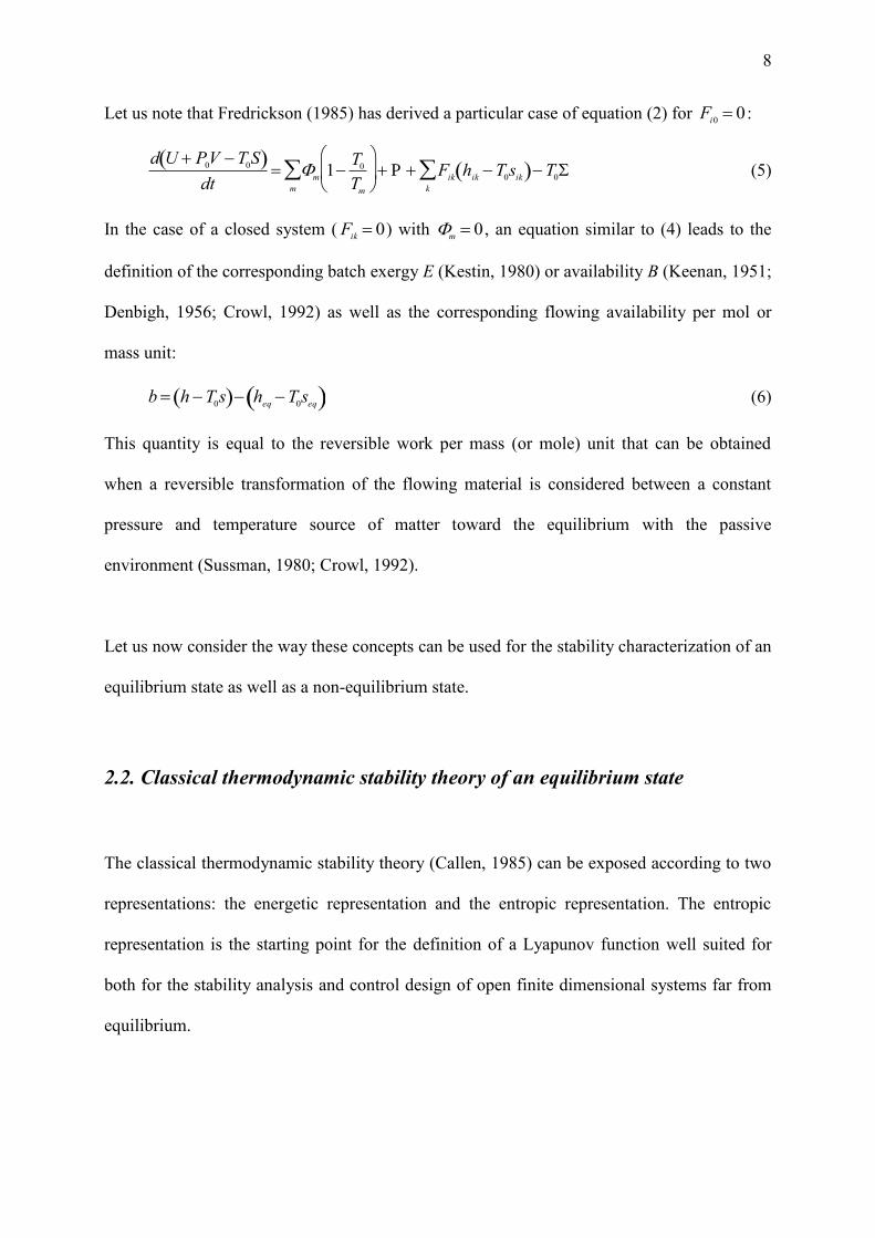
Let us note that Fredrickson (1985) has derived a particular case of equation (2) for

Fi0 0 :

d U P0V T

0S

dt

m1

T0

Tm

m

P Fik

hikT

0s

ik k

T0 (5)

In the case of a closed system (

Fik 0) with

m 0 , an equation similar to (4) leads to the

definition of the corresponding batch exergy E (Kestin, 1980) or availability B (Keenan, 1951;

Denbigh, 1956; Crowl, 1992) as well as the corresponding flowing availability per mol or

mass unit:

b h T0s h

eqT

0s

eq (6)

This quantity is equal to the reversible work per mass (or mole) unit that can be obtained

when a reversible transformation of the flowing material is considered between a constant

pressure and temperature source of matter toward the equilibrium with the passive

environment (Sussman, 1980; Crowl, 1992).

Let us now consider the way these concepts can be used for the stability characterization of an

equilibrium state as well as a non-equilibrium state.

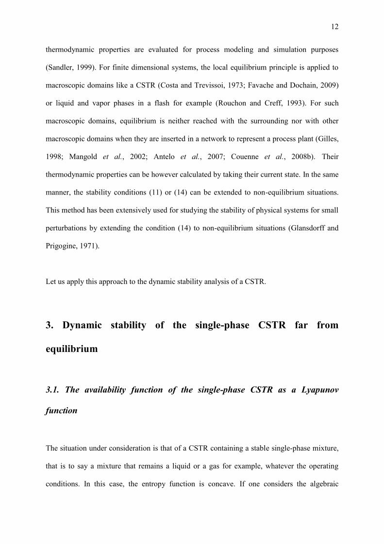
2.2. Classical thermodynamic stability theory of an equilibrium state

The classical thermodynamic stability theory (Callen, 1985) can be exposed according to two

representations: the energetic representation and the entropic representation. The entropic

representation is the starting point for the definition of a Lyapunov function well suited for

both for the stability analysis and control design of open finite dimensional systems far from

equilibrium.

9

2.2.1. Energetic representation

Let us consider a system initially at a thermodynamic equilibrium point characterized by the

intensive variables

Peq, T

eq,

ieq. These equilibrium variables are assumed to be constant so

that the situation can be treated by using equation (2) with

Fik 0,

m 0 and

P 0 and by

considering that the initial equilibrium situation is imposed by a passive environment at

P0 P

eq, T

0T

eq,

i0

ieq:

d U PeqV T

eqS

ieq

i

Ni

dt T

eq 0 (7)

The question is to determine if this initial equilibrium situation is dynamically stable with

respect to some fluctuations of the system state. According to equation (7), the system is

stable with respect to perturbations that lead to an increase of

U PeqV T

eqS

ieq

i

Ni .

Indeed, after the perturbation, the system is driven back to the equilibrium by irreversible

processes since ∑ > 0. An equivalent proposition is that the following inequality holds for a

stable system:

U PeqV T

eqS

ieq

i

NiU

eq P

eqV

eqT

eqS

eq

ieq

i

Nieq

(8)

where

Ueq P

eqV

eqT

eqS

eq

ieq

i

Nieq

is the value of the function

U PeqV T

eqS

ieq

i

Ni

when the system has reached equilibrium. Inequality (8) can also be written as follows:

U Ueq T

eqS S

eq Peq

V Veq

ieqN

iN

ieq i

(9)

According to the Gibbs equation applied to the equilibrium point,

dUeq

U

S

eq

dSeq

U

V

eq

dVeq

U

Ni

eq

dNieq

i

Teq

dSeq P

eqdV

eq

ieqdN

ieq

i

, the quantity

10

Ueq T

eqS S

eq Peq

V Veq

ieqN

iN

ieq i

is the equation of the tangent plane to the

internal energy surface

U S,V,Ni at the equilibrium point. From the inequality (9), it comes

that this function is convex for a stable equilibrium point (Callen, 1985).

2.2.2. Entropic representation

The inequality (9) can be written according to the entropy function as follows:

S Seq

1

Teq

U Ueq

Peq

Teq

V Veq

ieq

Teq

NiN

i eq i

(10)

By considering the corresponding Gibbs equation at the equilibrium point,

dSeq

S

U

eq

dUeq

S

V

eq

dVeq

S

Ni

eq

dNieq

i

dU

eq

Teq

P

eq

Teq

dVeq

ieq

Teq

dNieq

i

, the quantity

Seq

1

Teq

U Ueq

Peq

Teq

V Veq

ieq

Teq

NiN

i eq i

is the equation of the tangent plane to the

entropy surface

S U,V,Ni at the equilibrium point. From inequality (10), it comes that this

function is concave for a stable equilibrium point (Callen, 1985). Then, a finite algebraic

distance between the tangent plane to the entropy surface at the equilibrium point and the

entropy function can be defined as:

Seq

1

Teq

U Ueq

Peq

Teq

V Veq

ieq

Teq

NiN

i eq i

S

U1

Teq

1

T

V

Peq

Teq

P

T

N

i

ieq

Teq

i

T

i

0

(11)

This equation is obtained by considering

S S U,V,Ni as a first order homogeneous

function and by applying the Euler theorem at the equilibrium point (Sandler, 1999):

Seq

Ueq

Teq

P

eq

Teq

Veq

ieq

Teq

Nieq

i

(12)

11

If small perturbations are considered, equation (11) is equivalent to the second order Taylor

development of the entropy function:

S U,V ,Ni S

eq

S

U

eq

U S

V

eq

V S

Ni

eq

Ni

i

1

2

2S

U 2

eq

U 2

2S

V 2

eq

V 2

2S

NiN

k

eq

Ni N

k i ,k

2S

UV

eq

UV 2S

UNi

eq

UNi

i

2S

VNi

eq

VNi

i

(13)

The quantity

Seq

S

U

eq

U S

V

eq

V S

Ni

eq

Ni

i

is the tangent plane equation as

expressed locally so that the following local stability condition can be derived that is

equivalent to condition (11) for small perturbations (Kondepudi and Prigogine, 1998):

1

2 2S

1

2

2S

U 2

eq

U 2

2S

V 2

eq

V 2

2S

NiN

k

eq

Ni N

k i ,k

2S

UV

eq

UV 2S

UNi

eq

UNi

i

2S

VNi

eq

VNi

i

0

(14)

In this case, the equilibrium point is locally stable and is said to be metastable. Let us now

consider the way the stability condition (11) as it has been obtained in the entropic

representation, can be extended to the stability studies of systems far from equilibrium.

2.3. Extension to open systems far from equilibrium

The equilibrium state stability condition (11) has been used to derive a general condition that

the entropy state function

S S U,V,Ni should satisfy if an equilibrium point is assumed to

be stable. This condition is that the entropy function

S S U,V,Ni is concave. According to

the local equilibrium principle (De Groot and Mazur, 1984), such a function can also be used

to calculate the entropy of a system far from equilibrium. This is the ordinary way

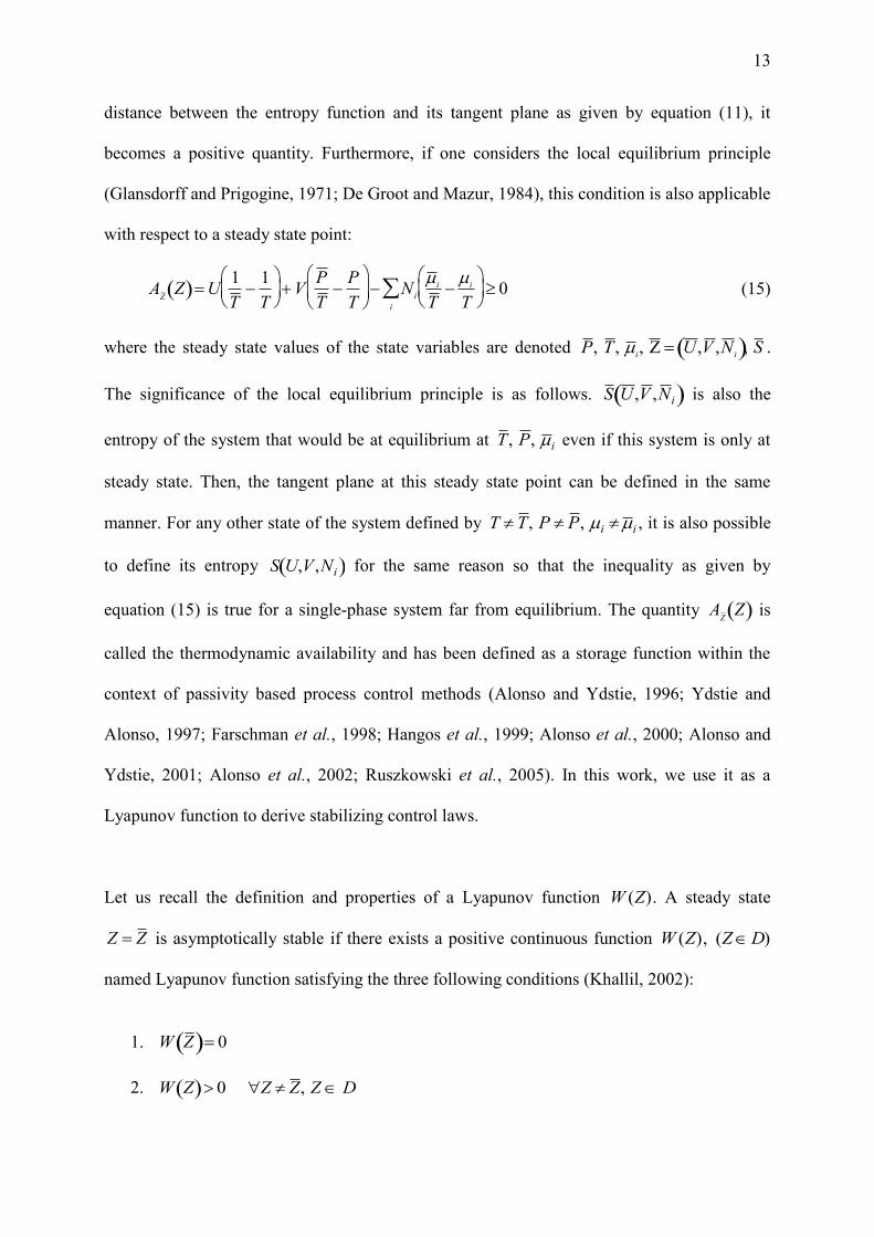
12

thermodynamic properties are evaluated for process modeling and simulation purposes

(Sandler, 1999). For finite dimensional systems, the local equilibrium principle is applied to

macroscopic domains like a CSTR (Costa and Trevissoi, 1973; Favache and Dochain, 2009)

or liquid and vapor phases in a flash for example (Rouchon and Creff, 1993). For such

macroscopic domains, equilibrium is neither reached with the surrounding nor with other

macroscopic domains when they are inserted in a network to represent a process plant (Gilles,

1998; Mangold et al., 2002; Antelo et al., 2007; Couenne et al., 2008b). Their

thermodynamic properties can be however calculated by taking their current state. In the same

manner, the stability conditions (11) or (14) can be extended to non-equilibrium situations.

This method has been extensively used for studying the stability of physical systems for small

perturbations by extending the condition (14) to non-equilibrium situations (Glansdorff and

Prigogine, 1971).

Let us apply this approach to the dynamic stability analysis of a CSTR.

3. Dynamic stability of the single-phase CSTR far from

equilibrium

3.1. The availability function of the single-phase CSTR as a Lyapunov

function

The situation under consideration is that of a CSTR containing a stable single-phase mixture,

that is to say a mixture that remains a liquid or a gas for example, whatever the operating

conditions. In this case, the entropy function is concave. If one considers the algebraic

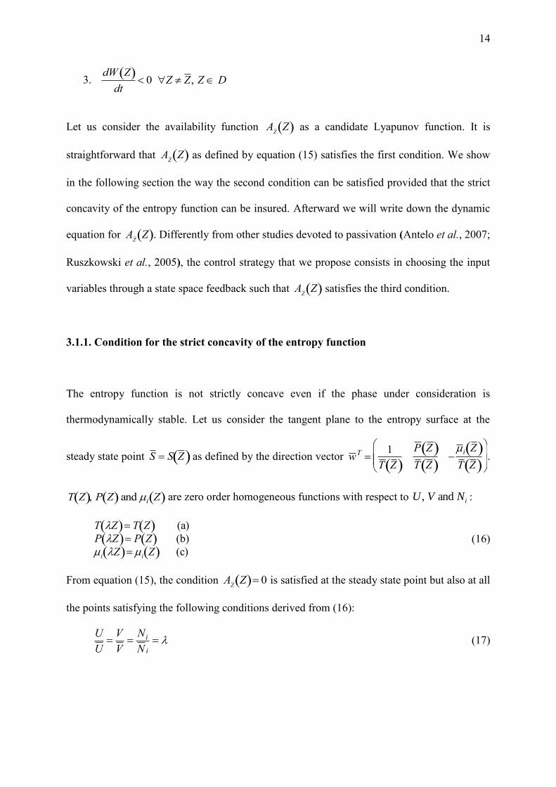
13

distance between the entropy function and its tangent plane as given by equation (11), it

becomes a positive quantity. Furthermore, if one considers the local equilibrium principle

(Glansdorff and Prigogine, 1971; De Groot and Mazur, 1984), this condition is also applicable

with respect to a steady state point:

AZ

Z U1

T

1

T

V

P

T

P

T

N

i

i

T

i

T

i

0 (15)

where the steady state values of the state variables are denoted

P , T , i, Z U ,V ,N

i , S .

The significance of the local equilibrium principle is as follows.

S U ,V ,N i is also the

entropy of the system that would be at equilibrium at

T , P , i even if this system is only at

steady state. Then, the tangent plane at this steady state point can be defined in the same

manner. For any other state of the system defined by

T T , P P , i i , it is also possible

to define its entropy

S U,V,Ni for the same reason so that the inequality as given by

equation (15) is true for a single-phase system far from equilibrium. The quantity

AZ

Z is

called the thermodynamic availability and has been defined as a storage function within the

context of passivity based process control methods (Alonso and Ydstie, 1996; Ydstie and

Alonso, 1997; Farschman et al., 1998; Hangos et al., 1999; Alonso et al., 2000; Alonso and

Ydstie, 2001; Alonso et al., 2002; Ruszkowski et al., 2005). In this work, we use it as a

Lyapunov function to derive stabilizing control laws.

Let us recall the definition and properties of a Lyapunov function

W (Z). A steady state

Z Z is asymptotically stable if there exists a positive continuous function

W (Z),

(ZD)

named Lyapunov function satisfying the three following conditions (Khallil, 2002):

1.

W Z 0

2.

W Z 0 Z Z , Z D

14

3.

dW Z dt

0 Z Z , Z D

Let us consider the availability function

AZ

Z as a candidate Lyapunov function. It is

straightforward that

AZ

Z as defined by equation (15) satisfies the first condition. We show

in the following section the way the second condition can be satisfied provided that the strict

concavity of the entropy function can be insured. Afterward we will write down the dynamic

equation for

AZ

Z . Differently from other studies devoted to passivation (Antelo et al., 2007;

Ruszkowski et al., 2005), the control strategy that we propose consists in choosing the input

variables through a state space feedback such that

AZ

Z satisfies the third condition.

3.1.1. Condition for the strict concavity of the entropy function

The entropy function is not strictly concave even if the phase under consideration is

thermodynamically stable. Let us consider the tangent plane to the entropy surface at the

steady state point

S S Z as defined by the direction vector

w T 1

T Z

P Z T Z

i Z T Z

.

T Z , P Z and i Z are zero order homogeneous functions with respect to iNVU and , :

T Z T Z (a)

P Z P Z (b)

i Z i Z (c)

(16)

From equation (15), the condition

AZ

Z 0 is satisfied at the steady state point but also at all

the points satisfying the following conditions derived from (16):

U

U

V

V

Ni

N i

(17)

15

In order the entropy to be strictly concave and the condition

AZ

Z 0 to be satisfied only at

the steady state point, at least one constraint on the extensive properties has to be imposed

(Jillson and Ydstie, 2007). Let us take a simple example to illustrate this point.

Example: Let us consider the mixing entropy

Sidm

of a binary ideal solution (Sandler, 1999):

Sidm Rln

N1

N1 N2

N1 Rln

N2

N1 N2

N2 (18)

One can verify that

Sidm

is a first order concave homogeneous function with respect to 1N

and 2N and that

Sidm

N1

Sidm

N2

R ln

N1

N1 N2

R ln

N2

N1 N2

are zero order

homogeneous functions with respect to 1N and 2N . The

Sidm

surface is represented in Figure

1. The algebraic distance

A N1,N2 between the tangent plane to the

Sidm

surface at

N1 N

1N

2 N

2 and the function

Sidm N1,N2 is given by:

0lnlnlnln

,

2

21

2

21

2

1

21

1

21

1

21

NNN

N

NN

NRN

NN

N

NN

NR

NNA

(19)

One can easily verify that

A N 1,N

2 A N 1,N

2 0. The condition

A 0 is then satisfied

on the contact line between the entropy surface and its tangent plane including

N 1

N 2 as

well as the origin )0,0( as it is shown in figure 1(a). If a constraint is imposed to the extensive

state variables, for example constant 21 NN (or constant 21 MM ,

constant 21 VV …), the entropy surface becomes a strictly concave line and the point

Z N 1

N 2 is the unique one that satisfies

A N 1,N

2 0 (see Figure 1(b)).

16

3.1.2. Derivation of

dAZ

dt for the CSTR with reaction networks

From equation (15), the following equations can be written for the differential of

AZ

Z that

is a first order homogeneous function with respect to

U,V,Ni:

dAZ dU

1

T

1

T

dV

P

T

P

T

dN i

iT i

T

(a)

i

dAZ

dt

dU

dt

1

T

1

T

dV

dt

P

T

P

T

dN i

dt

iT i

T

(b)

i

(20)

In order to derive the expression of

dAZ

dt, one has to consider the balance equations as

follows:

dU

dt Fi

inhi

in

i

Fi

outhi

out

i

0 P0l t dis (a)

dV

dt l t (b)

dN i

dt Fi

in Fi

out i

rrv

rVr

(c)

(21)

where tl is the volume time variation and

dis is an extra term accounting for possible

mechanical dissipation. The molar flow rate of component i is denoted

Fi, the superscripts in

and out standing for inlet and outlet flows. The volume of the system can vary with respect to

the surrounding at

P0. Heat transfer can occur with an external heat source at

T0.

rv

r is the rate

per volume unit of the rth

reaction and

i

r is the stoichiometric coefficient of the component i

when it is involved in the rth

reaction. In the case of a gas phase, the volume variation can be

due to the displacement of a piston. For example, new chemical reactors have recently been

described where a free piston is moving within a cylinder (Roestenberg et al., 2010). The

l t

function is then related to the piston motion. In the case of a liquid phase, the volume can vary

due to the evolution of the total number of moles of the mixture or to the variation of its molar

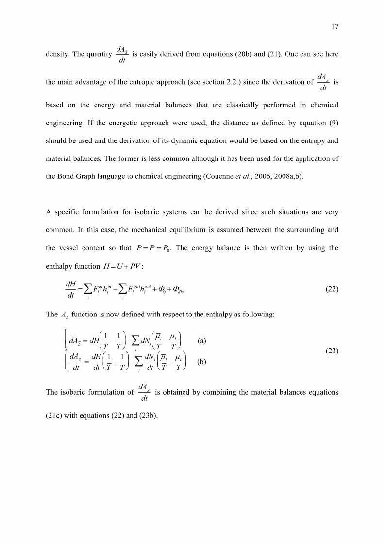
17

density. The quantity

dAZ

dt is easily derived from equations (20b) and (21). One can see here

the main advantage of the entropic approach (see section 2.2.) since the derivation of

dAZ

dt is

based on the energy and material balances that are classically performed in chemical

engineering. If the energetic approach were used, the distance as defined by equation (9)

should be used and the derivation of its dynamic equation would be based on the entropy and

material balances. The former is less common although it has been used for the application of

the Bond Graph language to chemical engineering (Couenne et al., 2006, 2008a,b).

A specific formulation for isobaric systems can be derived since such situations are very

common. In this case, the mechanical equilibrium is assumed between the surrounding and

the vessel content so that

P P P0. The energy balance is then written by using the

enthalpy function

H U PV :

dH

dt Fi

inhi

in

i

Fi

outhi

out

i

0 dis (22)

The

AZ function is now defined with respect to the enthalpy as following:

dAZ dH

1

T

1

T

dN i

iT i

T

(a)

i

dAZ

dt

dH

dt

1

T

1

T

dN i

dt

iT i

T

(b)

i

(23)

The isobaric formulation of

dAZ

dt is obtained by combining the material balances equations

(21c) with equations (22) and (23b).

18

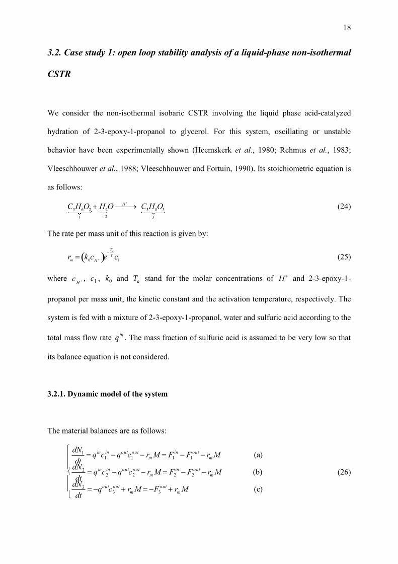
3.2. Case study 1: open loop stability analysis of a liquid-phase non-isothermal

CSTR

We consider the non-isothermal isobaric CSTR involving the liquid phase acid-catalyzed

hydration of 2-3-epoxy-1-propanol to glycerol. For this system, oscillating or unstable

behavior have been experimentally shown (Heemskerk et al., 1980; Rehmus et al., 1983;

Vleeschhouwer et al., 1988; Vleeschhouwer and Fortuin, 1990). Its stoichiometric equation is

as follows:

C3H

6O

2

1

H2O

2

H

C3H

8O

3

3

(24)

The rate per mass unit of this reaction is given by:

rm k

0c

H e

Ta

T c1 (25)

where

cH ,

c1 ,

k0 and aT stand for the molar concentrations of

H and 2-3-epoxy-1-

propanol per mass unit, the kinetic constant and the activation temperature, respectively. The

system is fed with a mixture of 2-3-epoxy-1-propanol, water and sulfuric acid according to the

total mass flow rate

qin. The mass fraction of sulfuric acid is assumed to be very low so that

its balance equation is not considered.

3.2.1. Dynamic model of the system

The material balances are as follows:

dN1

dt qinc1

in qoutc1

out rm M F1

in F1

out rm M (a)

dN2

dt qinc2

in qoutc2

out rm M F2

in F2

out rm M (b)

dN3

dt qoutc3

out rm M F3

out rm M (c)

(26)

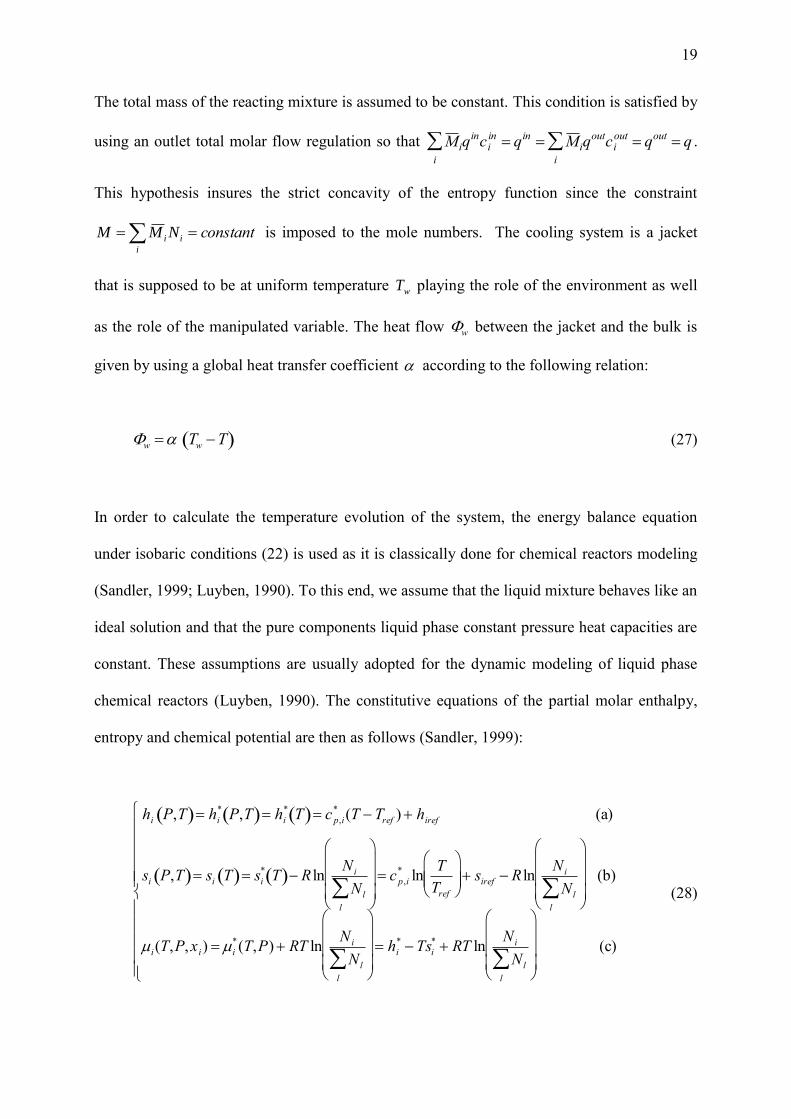
19

The total mass of the reacting mixture is assumed to be constant. This condition is satisfied by

using an outlet total molar flow regulation so that

M iqinci

in

i

qin M iqoutci

out

i

qout q .

This hypothesis insures the strict concavity of the entropy function since the constraint

constanti

ii NMM is imposed to the mole numbers. The cooling system is a jacket

that is supposed to be at uniform temperature wT playing the role of the environment as well

as the role of the manipulated variable. The heat flow

w between the jacket and the bulk is

given by using a global heat transfer coefficient according to the following relation:

w Tw T (27)

In order to calculate the temperature evolution of the system, the energy balance equation

under isobaric conditions (22) is used as it is classically done for chemical reactors modeling

(Sandler, 1999; Luyben, 1990). To this end, we assume that the liquid mixture behaves like an

ideal solution and that the pure components liquid phase constant pressure heat capacities are

constant. These assumptions are usually adopted for the dynamic modeling of liquid phase

chemical reactors (Luyben, 1990). The constitutive equations of the partial molar enthalpy,

entropy and chemical potential are then as follows (Sandler, 1999):

hi P,T hi

* P,T hi

* T c p,i

* (T Tref ) hiref (a)

si P,T si T si

* T R lnN i

N l

l

c p,i

* lnT

Tref

siref R ln

N i

N l

l

(b)

i(T,P, x i) i

*(T,P) RT lnN i

N l

l

hi

* Tsi

* RT lnN i

N l

l

(c)

(28)

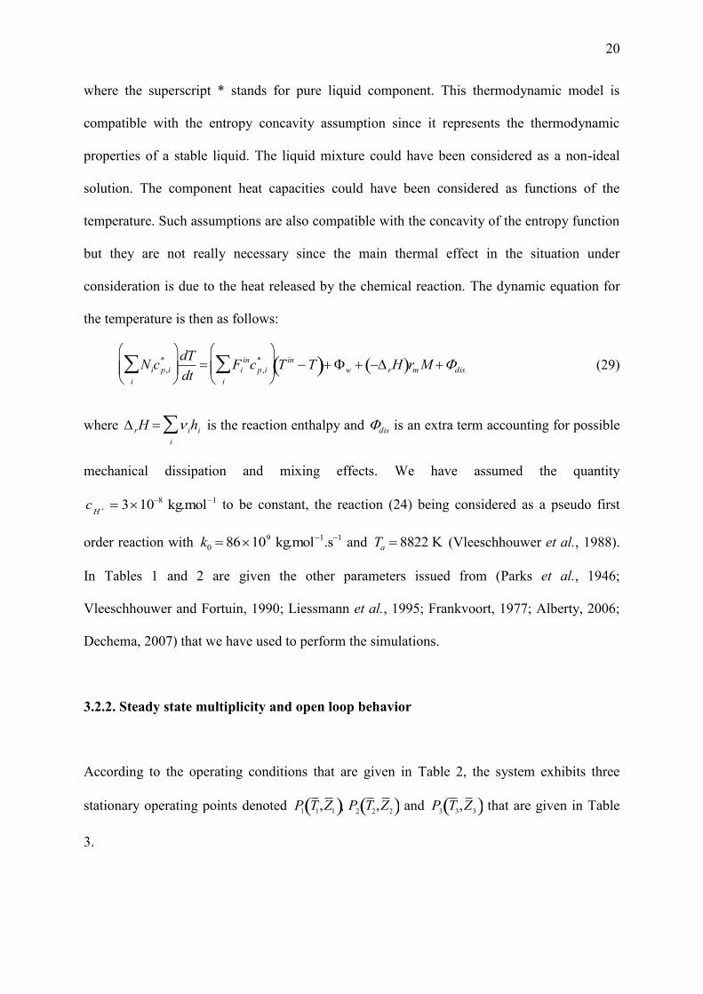
20

where the superscript * stands for pure liquid component. This thermodynamic model is

compatible with the entropy concavity assumption since it represents the thermodynamic

properties of a stable liquid. The liquid mixture could have been considered as a non-ideal

solution. The component heat capacities could have been considered as functions of the

temperature. Such assumptions are also compatible with the concavity of the entropy function

but they are not really necessary since the main thermal effect in the situation under

consideration is due to the heat released by the chemical reaction. The dynamic equation for

the temperature is then as follows:

Nic p,i

*

i

dT

dt Fi

incp,i

*

i

T

in T w rH rm M dis (29)

where

rH ihi

i

is the reaction enthalpy and

dis is an extra term accounting for possible

mechanical dissipation and mixing effects. We have assumed the quantity

cH 3108 kg.mol1 to be constant, the reaction (24) being considered as a pseudo first

order reaction with

k0 86109 kg.mol1.s1 and

Ta 8822 K (Vleeschhouwer et al., 1988).

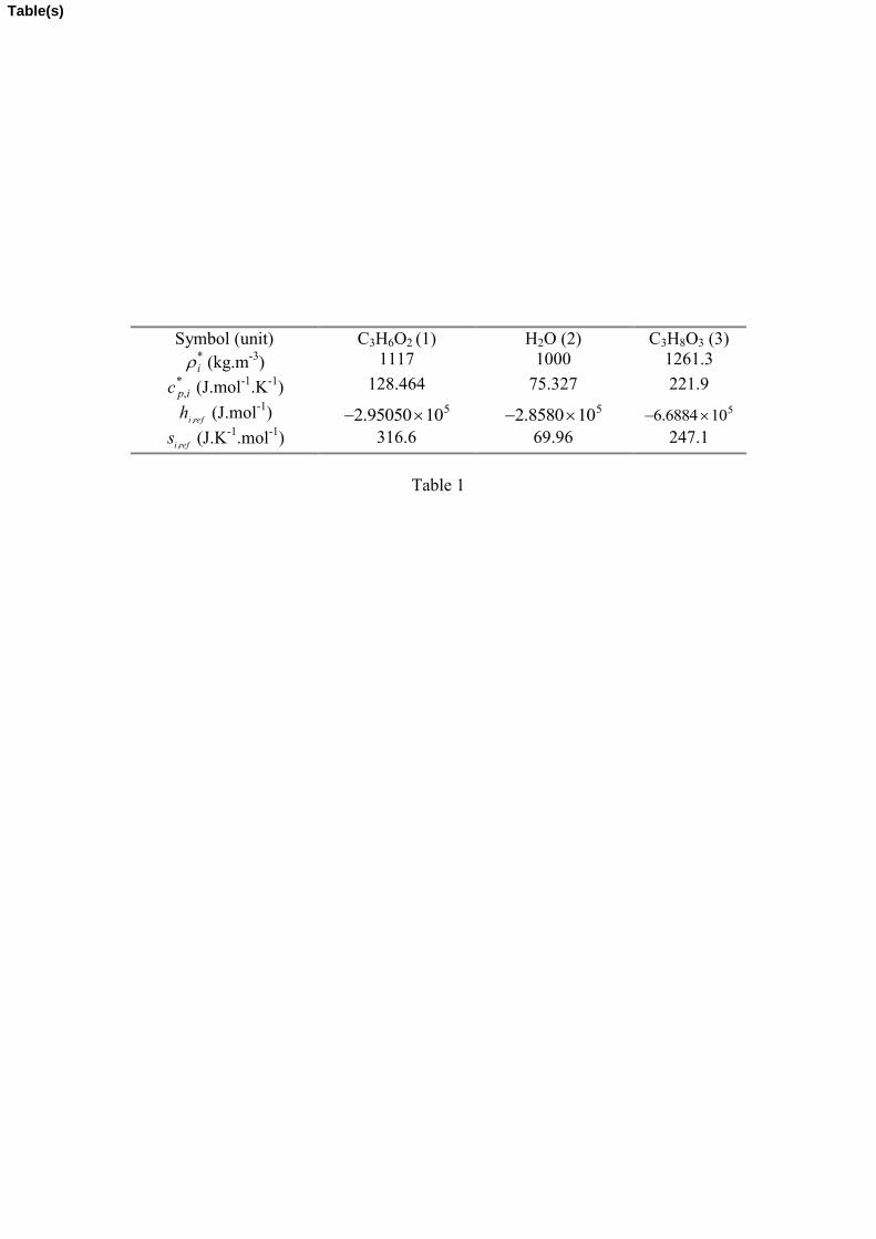
In Tables 1 and 2 are given the other parameters issued from (Parks et al., 1946;

Vleeschhouwer and Fortuin, 1990; Liessmann et al., 1995; Frankvoort, 1977; Alberty, 2006;

Dechema, 2007) that we have used to perform the simulations.

3.2.2. Steady state multiplicity and open loop behavior

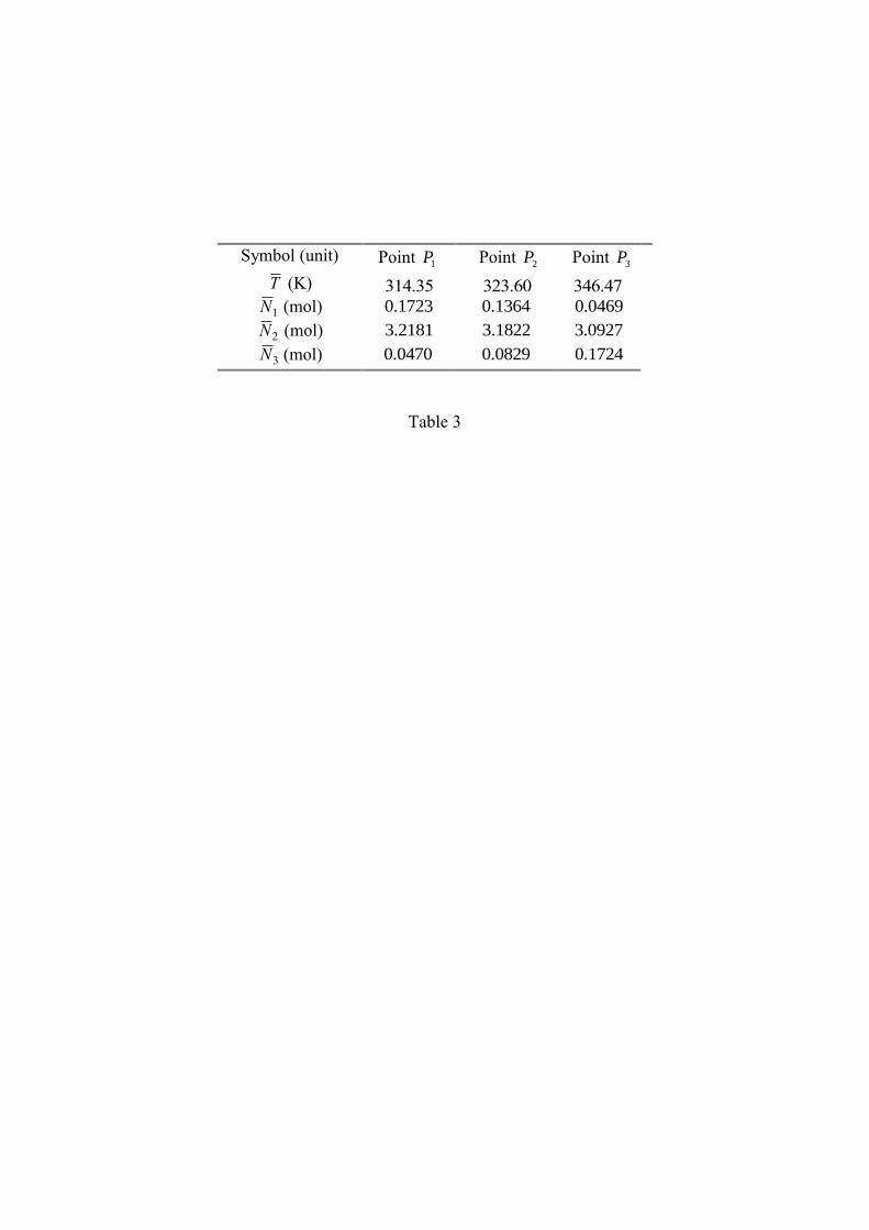
According to the operating conditions that are given in Table 2, the system exhibits three

stationary operating points denoted

P1

T 1,Z

1 , P2T

2,Z

2 and

P3

T 3,Z

3 that are given in Table

3.

21

The simulations results presented in the phase plane

N1,T in Figure 2 show that

P1 and 3P

are stable and 222 ,ZTP is unstable. It can be noted that some trajectories miss narrowly 2P

and finally reach 3P . The behavior of the availability function

AZ 1

Z given in Figure 3 from

the four initial conditions as given in Table 4 is that of a natural Lyapunov function for three

of them ),,( 431 CCC since it is decreasing until

limZZ 1

AZ 1

Z 0 . The curves issued from 3C and

4C are superimposed. The fourth curve issued from 2C corresponds to the curve that

asymptotically reaches 3P . As a consequence, 0lim1

3

ZAZZZ

but one can easily check that

0lim3

3

ZAZZZ

. It can be noted that in all the cases, the availability remains positive.

Since the point

P3 also corresponds to a stable operating point, simulation results are not

presented. Let us now consider the steady state point

P2. Dynamic simulations are performed

by considering the same aforementioned initial conditions. The simulations shown in Figure 4

illustrate the fact that the point

P2 is unstable since all these trajectories are such that

AZ 2

(Z)

does not asymptotically tend to zero. The final value of the availability depends on the

reached stationary points

P1 or

P3. Finally the availability from 2C comes close to zero when

the trajectory in the phase plan goes past

P2 (see Figure 2).

4. Application to the control of the liquid phase non-isothermal

CSTR: simulation studies

From the control point of view, since the availability is used as a Lyapunov function, it

remains to express the control input from state variables such that

22

dAZ (Z)

dt 0,Z Z , Z D. In the literature, the availability function is mostly used for a

posteriori stability analysis while the control strategy is achieved with classical PI or

nonlinear controllers (Antelo et al., 2007). In this paper we design the nonlinear controller

directly from the use of the availability function as a candidate Lyapunov function.

4.1. Design of a stabilizing feedback control law

In order to control the non-isothermal CSTR, the jacket temperature wT is chosen as the

manipulated variable (Viel et al., 1997; Alvarez-Ramirez and Puebla, 2001) according to the

industrial practice. It has been shown in previous works (Hoang, 2009; Hoang et al., 2008,

2009) that the feedback laws obtained from the condition

dAZ

Z dt

0 Z Z lead to

variations of the manipulated variable wT that cannot be realized in practice. Then, it has been

proposed to relax the initial control objective into

dAZ

T Z dt

0 Z Z where

AZ

T AZ A

Z

M

(

AZ

M being a positive function defined later on) captures the thermal part of the availability

(Hoang et al., 2012). In this case, asymptotic stability is insured with a physically admissible

manipulated variable in the vicinity of any desired steady state

T,Z , particularly in the case

of an open loop unstable point. So, let us assume the following closed loop control objective:

dAZ

T

dt K

1

T

1

T

2

(30)

with the constant

K 0.

23

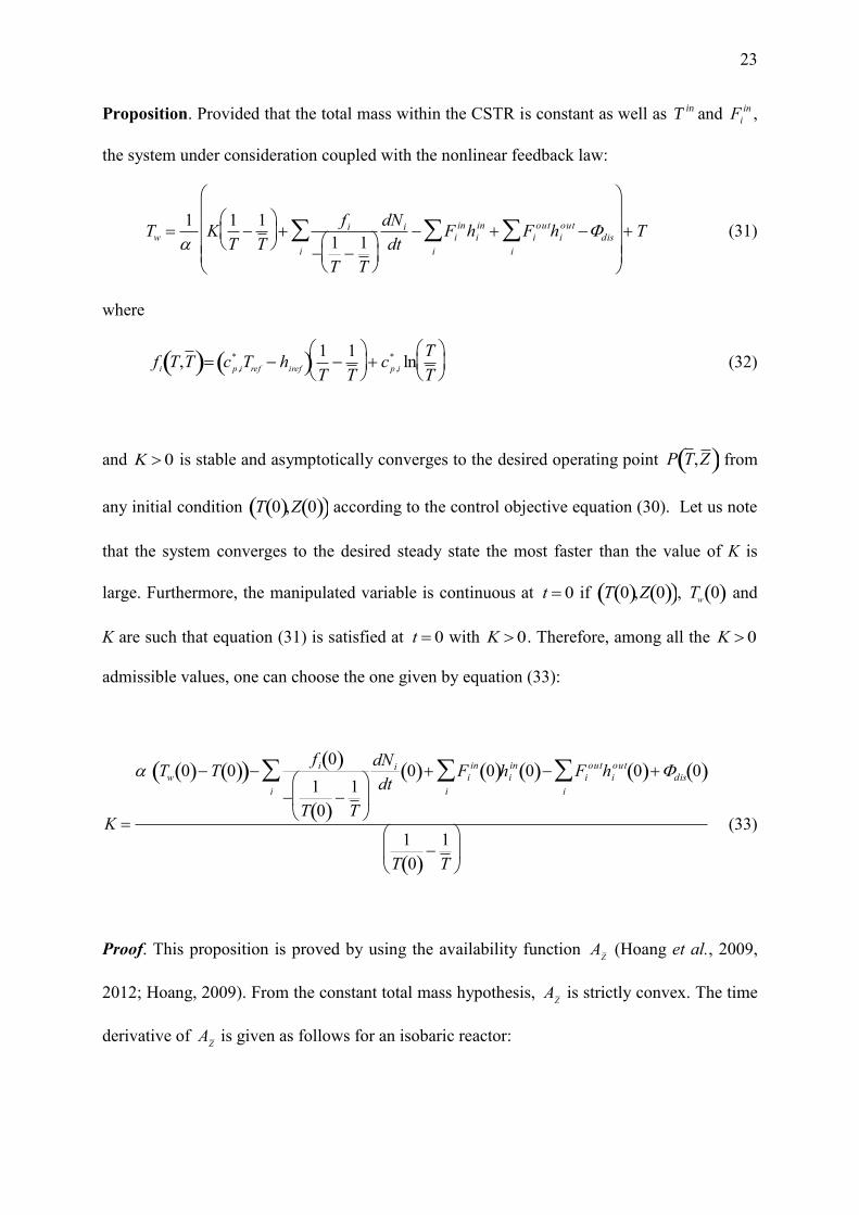
Proposition. Provided that the total mass within the CSTR is constant as well as inT and

Fi

in ,

the system under consideration coupled with the nonlinear feedback law:

Tw 1

K

1

T

1

T

f i

1

T

1

T

dN i

dti

Fi

in

i

hi

in Fi

out

i

hi

out dis

T (31)

where

fi

T,T cp ,i

* Tref h

iref 1

T

1

T

c

p ,i

* lnT

T

(32)

and

K 0 is stable and asymptotically converges to the desired operating point

P T,Z from

any initial condition

T 0 ,Z 0 according to the control objective equation (30). Let us note

that the system converges to the desired steady state the most faster than the value of K is

large. Furthermore, the manipulated variable is continuous at

t 0 if

T 0 ,Z 0 ,

Tw

0 and

K are such that equation (31) is satisfied at

t 0 with

K 0. Therefore, among all the

K 0

admissible values, one can choose the one given by equation (33):

K

Tw 0 T 0 f i 0

1

T 0

1

T

i

dN i

dt0 Fi

in 0 i

hi

in 0 Fi

out

i

hi

out 0 dis 0

1

T 0

1

T

(33)

Proof. This proposition is proved by using the availability function

AZ (Hoang et al., 2009,

2012; Hoang, 2009). From the constant total mass hypothesis,

AZ is strictly convex. The time

derivative of

AZ is given as follows for an isobaric reactor:

24

AZ

Z 1

T

1

T

H

iT i

T

i

N i (a)

dAZ

Z dt

1

T

1

T

dH

dt

iT i

T

i

dN i

dt (b)

(34)

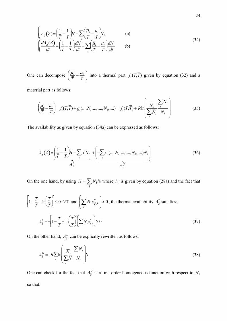
One can decompose

TT

ii into a thermal part

fi(T,T) given by equation (32) and a

material part as follows:

iT i

T

f i(T,T) gi(...,N l ,...,....,N l ,....) f i(T,T) R ln

N i

N ll

N l

l

N i

(35)

The availability as given by equation (34a) can be expressed as follows:

AZ

Z 1

T

1

T

H f i

i

N i

AZ

T

gi

i

(...,N l ,...,....,N l,....)N i

AZ

M

(36)

On the one hand, by using i

iihNH where ih is given by equation (28a) and the fact that

1T

T ln

T

T

0 T and 0*

,

i

ipicN , the thermal availability

AZ

T satisfies:

AZ

T 1T

T ln

T

T

N

ic

p ,i

*

i

0 (37)

On the other hand,

AZ

M can be explicitly rewritten as follows:

AZ

M -R lnN

i

N l

l

Nl

l

Ni

i

Ni (38)

One can check for the fact that

AZ

M is a first order homogeneous function with respect to

N i

so that:

25

dAZ

M

dt - g

i

i

dN

i

dt (39)

By combining equations (34b) and (39), we obtain:

dAZ

T

dt

1

T

1

T

dH

dt f

i

i

dN

i

dt (40)

By using the energy balance equation (22), we obtain from equation (40):

dAZ

T

dt

1

T

1

T

Fi

inhi

in

i

Fi

outhi

out

i

(Tw T)dis

f i

dNi

dti

(41)

One can check that by including the feedback law (31) in equation (41), the control objective

equation (30) is satisfied.

Remark 1.

AZ

M is also positive:

AZ

M R lnN

i

Nl

l

i

Ni R ln

N i

N l

l

i

Ni 0

AZ

M is the distance between the strictly convex first order homogeneous function with respect

to

N i ,

R lnN i

N l

l

i

N i and its tangent plane at

N i . Strict convexity is due again to constant

total mass assumption.

Remark 2. The stabilization obtained by using

dAZ

T

dt (Hoang, 2009; Hoang et al., 2008, 2009,

2012) leads to smooth time responses of the system and feasible trajectories of the

manipulated variable because

TT

f i

11 in equation (31) is a smooth function and as already

26

mentionned TT only when ZZ . Such a condition is not satisfied when the total

availability

AZ is used as in (Hoang et al., 2008).

4.2. Case study 1: closed loop stabilization of chemical reactors operating

under multiple steady states

This problem is illustrated by the liquid phase acid-catalyzed hydration of 2-3-epoxy-1-

propanol to glycerol as described in the section 3.2. In this case, there is only one reaction and

it can be shown that, as soon as

K 0, the time derivative of the temperature is monotonous

increasing or monotonous decreasing following that the initial temperature is greater or

smaller than the target temperature. Furthermore, it can be shown that there is only one steady

state temperature corresponding to a given set of stationary mole numbers. Consequently,

thanks to the Lasalle theorem (Khallil, 2002), the invariant set associated to

dAZ

T

dt 0 reduces

to Z so the trajectories converge asymptotically to Z and the control remains bounded.

In Figure 5, the total availability

AZ 2

Z is drawn in the case of a proportional controller

(noted P in what follows) of the form:

Tw k

pT T

2 (42)

associated to the perfect feedback on outlet flow rate. We recall this latter control enables the

strict concavity of entropy to be satisfied. A proportional integral (PI) controller does not

improve the stabilization property. The availability function is drawn for the four initial

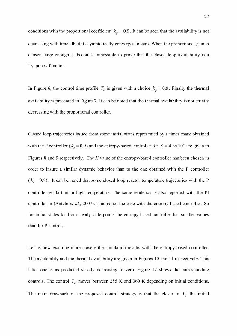
27

conditions with the proportional coefficient 9.0pk . It can be seen that the availability is not

decreasing with time albeit it asymptotically converges to zero. When the proportional gain is

chosen large enough, it becomes impossible to prove that the closed loop availability is a

Lyapunov function.

In Figure 6, the control time profile

Tw is given with a choice 9.0pk . Finally the thermal

availability is presented in Figure 7. It can be noted that the thermal availability is not strictly

decreasing with the proportional controller.

Closed loop trajectories issued from some initial states represented by a times mark obtained

with the P controller (

kp 0,9) and the entropy-based controller for 4103.4 K are given in

Figures 8 and 9 respectively. The K value of the entropy-based controller has been chosen in

order to insure a similar dynamic behavior than to the one obtained with the P controller

(

kp 0,9). It can be noted that some closed loop reactor temperature trajectories with the P

controller go farther in high temperature. The same tendency is also reported with the PI

controller in (Antelo et al., 2007). This is not the case with the entropy-based controller. So

for initial states far from steady state points the entropy-based controller has smaller values

than for P control.

Let us now examine more closely the simulation results with the entropy-based controller.

The availability and the thermal availability are given in Figures 10 and 11 respectively. This

latter one is as predicted strictly decreasing to zero. Figure 12 shows the corresponding

controls. The control wT moves between 285 K and 360 K depending on initial conditions.

The main drawback of the proposed control strategy is that the closer to 2P the initial

28

condition is, the higher the control is. It is compensated by the fact it is possible to easily

compute the tuning parameter K such that the control wT be continuous at

t 0 as stated in

equation (32) (in this case the K value is directly derived from the initial conditions). Indeed

the domain of initial conditions for which the system can be stabilized with a control variable

continuous at 0t is larger in the case of Lyapunov-based control than in the case of

proportional control. With these choices the control variable range between 293 K and 330 K

as shown in Figure 13. Finally let us note that such an adaptation cannot be performed with a

proportional controller.

4.3. Case study 2: optimization and control of multiple reactions system

with non-minimum phase behaviour

We consider a liquid phase non-isothermal CSTR where some series/parallel reactions take

place. The proposed control strategies can be applied to this multiple chemical reactions

system. One has only to assume that the isothermal open loop dynamics has a unique

stationary point at

T T ; if it is the case, it immediately follows that if

T tends to T then Z

tends to Z and the control is well defined.

More precisely, we are interested in the reaction for the production of cyclopentenol ( 2S )

from cyclopentadiene ( 1S ) by acid-catalyzed electrophilic addition of water in dilute solution

(Engell and Klatt, 1993; Niemiec and Kravaris, 2003; Antonelli and Astolfi, 2003; Guay et

al., 2005; Chen and Peng, 2006; Ramírez et al., 2009). Such a process is described by the

well-known Van de Vusse reactions system (Van de Vusse, 1964) and can be written as

follows:

29

C5H6

S1

H2O

S5

k1 / H

C5H7OH

S2

C5H7OH

S2

H2O

S5

k2 / H

C5H8(OH)2

S3

2C5H6

S1

k3 C10H12

S4

(43)

where 1S is the reactant, 2S is the desired product and 3S and 4S are unwanted by-products.

5S and 6S are water and catalyst/sulfuric acid respectively. The system dynamic model is

derived from the material and energy balance equations (Engell and Klatt, 1993; Niemiec and

Kravaris, 2003) where the molar concentrations per mass unit

c i N i

M have been used:

MM

NTkHM

M

NTkH

MM

NTkHTT

M

cq

dt

dTcN

NM

q

M

q

dt

dN

MM

NTkM

M

NTkN

M

q

M

q

dt

dN

MM

NTkN

M

q

dt

dN

MM

NTkN

M

q

dt

dN

MM

NTkM

M

NTkN

M

q

dt

dN

MM

NTkM

M

NTkN

M

q

M

q

dt

dN

rr

rw

in

i i

ipin

i

i

ipi

in

in

in

2

133

222

111

6

1

*

,6

1

*

,

66

66

22

115

55

5

2

134

4

223

3

22

112

2

2

13

111

11

1

)()(

(g))(

(f)

(e) )()(

(d) )(

(c) )(

(b) )()(

(a) )(2)(

(44)

In equations (44), the chemical rates are also expressed on a mass basis. The molar number of

sulfuric acid is regulated to be constant in the reactor by imposing some appropriate initial

condition

N6(t 0) M

M 6

6

in

and let us note that the dynamical model (44) fulfills the

30

constraint on the total mass

M constant since

.066

22

11

dt

dNM

dt

dNM

dt

dNM

dt

dM We neglect the additive power

dis due to

possible mechanical dissipation and mixing effects in the energy balance equation (44g).

Kinetic and thermodynamic parameters are given in Tables 5 and 6 adapted from (Engell and

Klatt, 1993; Niemiec and Kravaris, 2003).

The control objective is to maintain the process output 2N as close as to a steady state set

point by adjusting the jacket temperature wT only.

4.3.1. Dynamical analysis and non-minimum phase behaviour

Let

N 1,N

2,T be possible steady states of the system (44). A mathematical analysis for such

states leads to:

(b)

)(4

)(8)()(

)(

)(

(a)

)(4

)(8)()(

_

3

11

_

3

2_

1

_

1

_

2

_

12

_

3

11

_

3

2_

1

_

1

1

M

Tk

M

q

M

TkTk

M

qTk

M

q

TkM

q

TkN

M

Tk

M

q

M

TkTk

M

qTk

M

q

N

in

in

(45)

and

(T_

,Tw ) q i

inc p,i

*

M ii1

6

T

in T_

Tw T

_

r1H(T

_

)

k1(T

_

)N_

1

r2H(T_

)

k2(T

_

)N2 r3H(T_

)

k3(T_

)

MN_

1

2

0

(46)

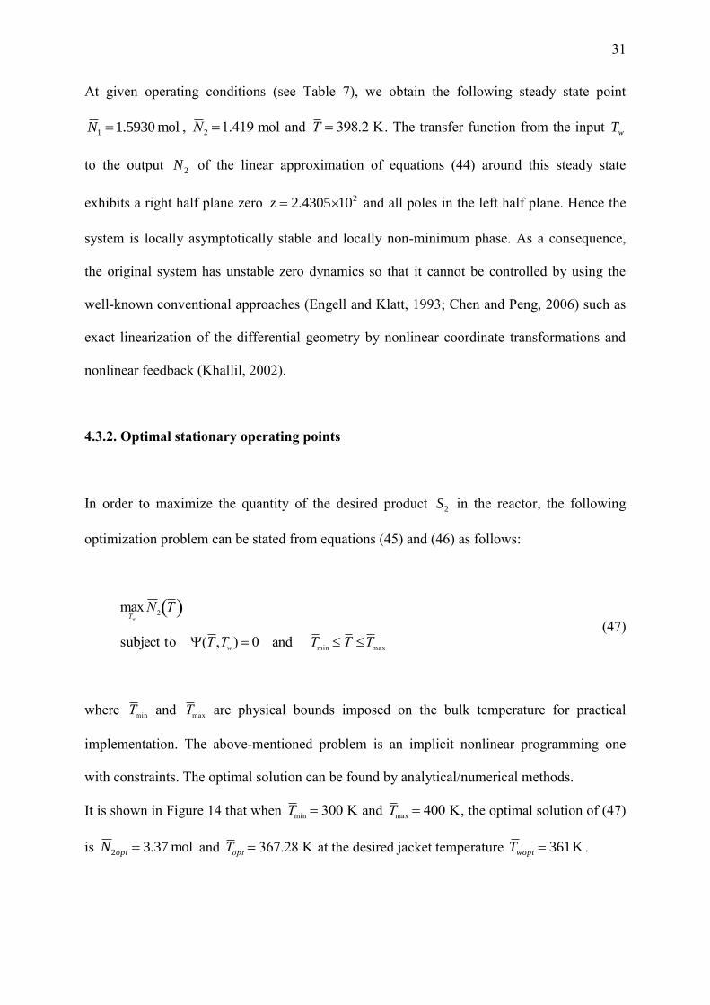
31

At given operating conditions (see Table 7), we obtain the following steady state point

mol 5930.11 N ,

N 2 1.419 mol and

T 398.2 K. The transfer function from the input wT

to the output 2N of the linear approximation of equations (44) around this steady state

exhibits a right half plane zero 2104305.2 z and all poles in the left half plane. Hence the

system is locally asymptotically stable and locally non-minimum phase. As a consequence,

the original system has unstable zero dynamics so that it cannot be controlled by using the

well-known conventional approaches (Engell and Klatt, 1993; Chen and Peng, 2006) such as

exact linearization of the differential geometry by nonlinear coordinate transformations and

nonlinear feedback (Khallil, 2002).

4.3.2. Optimal stationary operating points

In order to maximize the quantity of the desired product 2S in the reactor, the following

optimization problem can be stated from equations (45) and (46) as follows:

maxTw

N 2

T

subject to (T ,Tw) 0 and T

min T T

max

(47)

where

T min

and

T max

are physical bounds imposed on the bulk temperature for practical

implementation. The above-mentioned problem is an implicit nonlinear programming one

with constraints. The optimal solution can be found by analytical/numerical methods.

It is shown in Figure 14 that when

T min 300 K and

T max

400 K, the optimal solution of (47)

is mol 37.32 optN and

T opt 367.28 K at the desired jacket temperature K 361woptT .

32

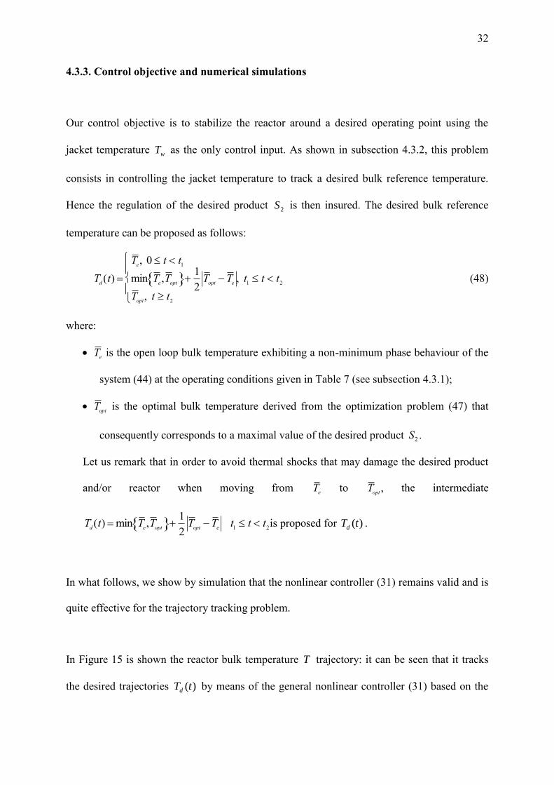
4.3.3. Control objective and numerical simulations

Our control objective is to stabilize the reactor around a desired operating point using the

jacket temperature wT as the only control input. As shown in subsection 4.3.2, this problem

consists in controlling the jacket temperature to track a desired bulk reference temperature.

Hence the regulation of the desired product 2S is then insured. The desired bulk reference

temperature can be proposed as follows:

Td(t)

T e, 0 t t

1

min T e,T

opt 1

2T

optT

e

T opt

, t t2

, t1 t t

2 (48)

where:

T e is the open loop bulk temperature exhibiting a non-minimum phase behaviour of the

system (44) at the operating conditions given in Table 7 (see subsection 4.3.1);

T opt

is the optimal bulk temperature derived from the optimization problem (47) that

consequently corresponds to a maximal value of the desired product

S2 .

Let us remark that in order to avoid thermal shocks that may damage the desired product

and/or reactor when moving from

T e to

T opt

, the intermediate

Td(t) min T

e,T

opt 1

2T

optT

e t

1 t t

2is proposed for )(tTd .

In what follows, we show by simulation that the nonlinear controller (31) remains valid and is

quite effective for the trajectory tracking problem.

In Figure 15 is shown the reactor bulk temperature T trajectory: it can be seen that it tracks

the desired trajectories )(tTd by means of the general nonlinear controller (31) based on the

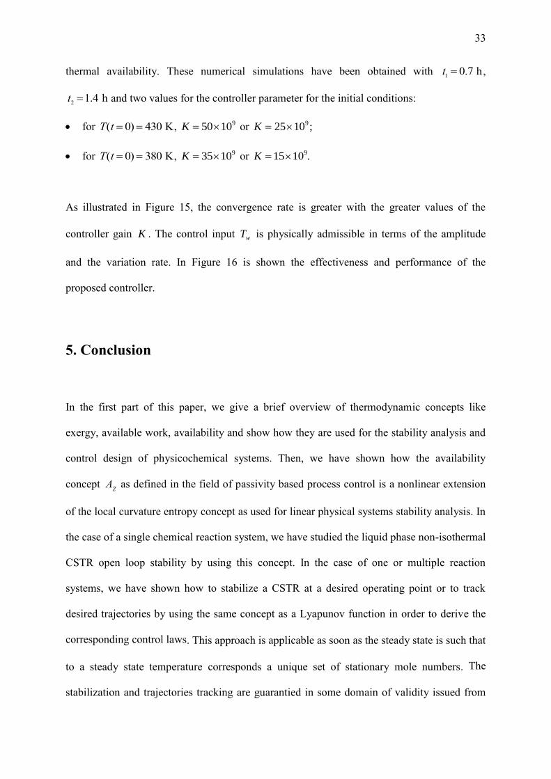
33

thermal availability. These numerical simulations have been obtained with

t1 0.7 h ,

t21.4 h and two values for the controller parameter for the initial conditions:

for

T(t 0) 430 K, 91050K or ;1025 9K

for

T(t 0) 380 K, 91035K or .1015 9K

As illustrated in Figure 15, the convergence rate is greater with the greater values of the

controller gain K . The control input wT is physically admissible in terms of the amplitude

and the variation rate. In Figure 16 is shown the effectiveness and performance of the

proposed controller.

5. Conclusion

In the first part of this paper, we give a brief overview of thermodynamic concepts like

exergy, available work, availability and show how they are used for the stability analysis and

control design of physicochemical systems. Then, we have shown how the availability

concept

AZ as defined in the field of passivity based process control is a nonlinear extension

of the local curvature entropy concept as used for linear physical systems stability analysis. In

the case of a single chemical reaction system, we have studied the liquid phase non-isothermal

CSTR open loop stability by using this concept. In the case of one or multiple reaction

systems, we have shown how to stabilize a CSTR at a desired operating point or to track

desired trajectories by using the same concept as a Lyapunov function in order to derive the

corresponding control laws. This approach is applicable as soon as the steady state is such that

to a steady state temperature corresponds a unique set of stationary mole numbers. The

stabilization and trajectories tracking are guarantied in some domain of validity issued from

34

the positivity condition of the design parameter K and the continuity of the feedback law for

wT . Some guidelines for the design of parameter K in terms of the trade-off between

performances and actuator solicitation are given. The proposed approach is illustrated via

simulation examples by using thermodynamic and kinetic data of chemical reactions that are

described in the literature. The simulation results show that stabilization is solved with

physically admissible time evolution of the jacket temperature used as the only manipulated

variable and compared with results obtained using a proportional feedback controller. It is

also shown that the stability region with the entropy-based controller is larger than the one

with P or PI controller. The range of the control values are of the same order with the two

controllers.

35

ACKNOWLEDGMENTS

This work is supported by the Vietnam's National Foundation for Science and Technology

Development (NAFOSTED) under research proposal number 101.01-2013.23. The scientific

responsibility rests with its authors.

36

NOMENCLATURE

ZA : availability (J.K

-1)

T

ZA : thermal part of the CSTR availability (J.K

-1)

M

ZA : material part of the CSTR availability (J.K

-1)

B: available work or exergy (J)

b: steady flow availability (J.mol-1

or J.kg-1

)

c: concentration (mol.kg-1

)

c p: constant pressure heat capacity (J.mol-1

.K-1

)

D: domain of variation for the extensive variables (-)

E: available work or exergy (J)

f: function involved in the expression of the thermal part of the availability (J.K-1

.mol-1

)

g: function involved in the expression of the material part of the availability (J.K-1

.mol-1

)

H: enthalpy (J)

rH : reaction enthalpy (J.mol-1

)

h: specific enthalpy (J.mol-1

or J.kg-1

)

k0 : kinetic contant (kg.mol-1

.s-1

)

K: controller parameter (-)

l(t): volume time variation (m3.s

-1)

M: mass (kg)

M : molar mass (kg.mol-1

)

N: number of mole (mol)

P: pressure (Pa)

P : power (W)

q: mass flow rate (kg.s-1

)

37

R: ideal gas constant (J.mol-1

.K-1

)

r: chemical reaction rate (mol.s-1

.m-3

or mol.s-1

.kg-1

)

S: entropy (J.K-1

)

s: specific entropy (J.K-1

.mol-1

or J.K-1

.kg-1

)

T: temperature (K)

t: time (s)

U: internal energy (J)

V: volume (m3)

W: Lyapunov function (-)

x: molar fraction (-)

wT: vector of intensives variables (-)

ZT: vector of extensive variables (-)

Greek symbols

: global heat transfer coefficient between CSTR jacket and bulk fluid (W.K-1

)

: homogeneity ratio (-)

: entropy production per time unit (J.K-1

.s-1

)

: heat flow (W)

: chemical potential (J.mol-1

)

: stoichiometric coefficient (-)

: mass density (kg.m-3

)

: mass fraction (-)

: variation of a quantity (-)

38

Subscript

a: activation

d: desired

dis: dissipation

eq: equilibrium

i, l: components i, l

0: passive environment or surrounding

opt: optimal

w: wall

k: system k

m: heat source or per unit of mass

v: per unit of volume

Superscript

X : steady-state value of X

in: inlet

out: outlet

r: rth

reaction

*: pure liquid component

39

Literature Cited

Alberty, R.A., 2006. Standard molar entropies, standard entropies of formation, and standard

transformed entropies of formation in the thermodynamics of enzyme-catalyzed reactions. J.

Chem. Thermodynamics 38, 396-404.

Alonso, A.A., Ydstie, B.E., 1996. Process systems, passivity and the second law of

thermodynamics. Computers and Chemical Engineering 20, 1119-1124.

Alonso, A.A., Banga, J.R., Sanchez, I., 2000. Passive control design for distributed process

systems: theory and applications. AIChE Journal 46, 1593–1606.

Alonso, A.A., Ydstie, B.E., 2001. Stabilization of distributed systems using irreversible

thermodynamics. Automatica 37, 1739–1755.

Alonso, A.A., Ydstie, B.E., Julio, R.B., 2002. From irreversible thermodynamics to a robust

control theory for distributed process systems. Journal of Process Control 12, 507–517.

Antelo, L.T., Otero-Muras, I., Banga, J.R., Alonso, A.A., 2007. A systematic approach to

plant-wide control based on thermodynamics. Computers & Chemical Engineering 31, 677-

691.

Alvarez-Ramirez, J., Puebla, H., 2001. On classical PI control of chemical reactors. Chemical

Engineering Science 56, 2111-2121.

Antonelli, R., Astolfi, A., 2003. Continuous stirred tank reactors: easy to stabilise?

Automatica 39, 1817-1827.

Aris, R., Amundson, N.R., 1958. An analysis of chemical reactor stability and control - I. The

possibility of local control, with perfect or imperfect control mechanisms. Chemical

Engineering Science 7, 121–131.

40

Bahroun, S., Li, S., Jallut, C., Valentin, C., de Panthou, F., 2010. Control and optimization of

a three-phase catalytic slurry intensified continuous chemical reactor. Journal of Process

Control 20(5), 664–675.

Bahroun, S., Couenne, F., Jallut, C., Valentin, C., 2013. Thermodynamic-based nonlinear

control of a three-phase slurry catalytic fed-batch reactor. IEEE Transactions on Control

Systems Technology 21(2), 360-371.

Batlle, C., Ortega, R., Sbarbaro, D., Ramírez, H., 2010. Corrigendum to ―On the control of

non-linear processes: An IDA-PBC approach‖. Journal of Process Control 20, 121-122.

Alvarez, J., Alvarez-Ramírez, J., Espinosa-Perez, G., Schaum, A., 2011. Energy shaping plus

damping injection control for a class of chemical reactors. Chemical Engineering Science

66(23), 6280-6286.

Bejan, A., 2006. Advanced Engineering Thermodynamics, 3rd

ed, Lavoisier, Paris.

Bequette B.W., 1991. Nonlinear control of chemical processes: A review. Ind. Eng. Chem.

Res. 30, 1391–1413.

Callen, H.B., 1985. Thermodynamics and an introduction to thermostatistics, 2nd

edition,

Wiley and Sons.

Chen, C.T., and Peng, S.T., 2006. A sliding model scheme for nonminimum phase non-linear

uncertain input-delay chemical process. Journal of Process Control 16, 37-51.

Costa, P., Trevissoi, C., 1973. Thermodynamic stability of chemical reactors. Chemical

Engineering Science 28, 2195-2203.

Couenne, F., Jallut, C., Maschke, B., Breedveld, P.C., Tayakout, M., 2006. Bond graph

modelling for chemical reactors. Mathematical and Computer Modelling of Dynamical

Systems 12, 159-174

41

Couenne, F., Jallut, C., Maschke, B., Tayakout, M., Breedveld, P.C., 2008a. Bond Graph for

dynamic modelling in chemical engineering. Chemical Engineering and Processing, 47, 1994-

2003.

Couenne, F., Jallut, C., Maschke, B., Tayakout, M., Breedveld, P., 2008b. Structured

modeling for processes: A thermodynamical network theory. Computers & Chemical

Engineering 32, 1120-1134.

Crowl, D.A., 1992. Calculating the energy of explosion using thermodynamic availability. J.

Loss Prev. Process Ind. 5, 109-118.

Dammers, W.R., Tels, M., 1974. Thermodynamic stability and entropy production in

adiabatic stirred flow reactors. Chemical Engineering Science 29(1), 83-90.

Dechema data-base Detherm 2.2.0, 2007.

De Groot, S.R., Mazur, P., 1984. Non-equilibrium thermodynamics, Dover.

Denbigh, K.G., 1956. The second law analysis of chemical processes. Chemical Engineering

Science 1, 1-9.

Engell, S., Klatt, K.U., 1993. Nonlinear control of a non-minimum-phase CSTR. American

Control Conference, pp. 2941-2945.

Farschman, C.A., Viswanath, K.P., Ydstie, B.E., 1998. Process systems and inventory

control. AIChE Journal 44, 1841-1857.

Favache, A., Dochain, D., 2009. Thermodynamics and chemical systems stability: the CSTR

case study revisited. Journal of Process Control 19, 371-379.

Favache, A., Dochain, D., 2010. Power-shaping of reaction systems: the CSTR case study.

Automatica 46(11), 1877-1883.

Frankvoort, W., 1977. An adiabatic reaction calorimeter for the determination of kinetic

constants of liquid reactions at high concentrations. Thermochimica Acta 21, 171-183.

42

Fredrickson, A.G., 1985. Reference states and balance equations for relative thermodynamic

properties, including availability. Chemical Engineering Science 40, 2095-2104.

Glansdorff, P., Prigogine, I., 1971. Thermodynamic theory of structure, stability and

fluctuations, Wiley-Interscience.

Georgakis, C., 1986. On the use of extensive variables in process dynamics and control.

Chemical Engineering Science 41, 1471-1484.

Gilles, E.D., 1998. Network theory for chemical processes. Chem. Eng. Technol. 21, 121-132.

Guay, M., Dochain, D., Perrier M., 2005. Adaptive extremum-seeking control of

nonisothermal continuous stirred tank reactors. Chemical Engineering Science 60, 3671-3681.

Hangos, K.M., Alonso, A.A., Perkins, J.D., Ydstie, B.E., 1999. Thermodynamic approach to

the structural stability of process plants. AIChE Journal 45, 802-816.

Heemskerk, A.H., Dammers, W.R., Fortuin, J.M.H., 1980. Limit cycles measured in a liquid-

phase reaction system. Chemical Engineering Science 32, 439-445.

Hoang, N.H., Couenne, F., Jallut, C., Le Gorrec, Y., 2008. Lyapunov based control for non

isothermal continuous stirred tank reactor, in: Proceedings of the 17th

World Congress of the

IFAC, Seoul, Korea, pp. 3854-3858.

Hoang, N.H., Couenne, F., Jallut, C., Le Gorrec, Y., 2009. Thermodynamic approach for

Lyapunov based control, in: Proceedings of the International Symposium on Advanced

Control of Chemical Processes, Istanbul, Turkey, pp. 367-372.

Hoang, N.H., 2009. Thermodynamic approach for the stabilization of chemical reactors (in

french), PhD thesis, Lyon University.

Hoang, H., Couenne, F., Jallut, C., Le Gorrec, Y. , 2012. Lyapunov-based control of non

isothermal continuous stirred tank reactors using irreversible thermodynamics. J. Proc.

Control 22(2), 412-422.

Jillson, K.R., Ydstie, B.E., 2007. Process networks with decentralized inventory and flow

43

control. Journal of Process Control 17, 399–413.

Keenan, J.H., 1951. Availability and irreversibility in thermodynamics. British Journal of

Applied Physics 2, 183-192.

Kestin, J., 1980. Availability: the concept and associated terminology. Energy 5, 679-692.

Khallil, H.K., 2002. Nonlinear systems, 3rd

edition, Prentice Hall.

Kondepudi, D., Prigogine, I., 1998. Modern thermodynamics. From heat engines to

dissipative structure, Wiley and Sons.

Liessmann, G., Schmidt, W., Reiffarth, S., 1995. Recommended Thermophysical Data in

―Data compilation of the Saechsische Olefinwerke Boehlen‖, Germany.

Luyben, W.L., 1990. Process modeling, simulation and control for chemical engineers, 2d

edition, McGraw-Hill.

Mangold, M., Motz, S., Gilles, E.D., 2002. A network theory for the structured modelling of

chemical processes. Chemical Engineering Science 57, 4099-4114.

Niemiec, M.P., Kravaris, C., 2003. Nonlinear model-state feedback control for a non-

minimum phase processes. Automatica 39, 1295-1302.

Parks, G.S., West, T.J., Naylor, B.F., Fujii, P.S., McClaine, L.A., 1946. Thermal data on

organic compounds. XXIII. Modern combustion data for fourteen Hydrocarbons and five

Polyhydroxy Alcohols. J. Am. Soc. 68, 2524-2727.

Perlmutter, D.D., 1972. Stability of chemical reactors, Prentice-Hall.

Ramírez, H., Sbarbaro, D., Romeo Ortega R., 2009. On the control of non-linear processes:

An IDA–PBC approach. J. Process Control 19, 405-414.

Rehmus, P., Zimmermann, E.C., Ross, J., 1983. The periodically forces conversion of 2-3-

epoxy-1-propanol to glycerine: a theoretical analysis. J. Chem. Phys. 78, 7241-7251.

44

Roestenberg, T., Glushenkov, M.J., Kronberg, A.E., Krediet, H.J., Meer, Th. H. vd., 2010.

Heat transfer study of the pulsed compression reactor. Chemical Engineering Science 65, 88-

91.

Rouchon, P., Creff, Y., 1993. Geometry of the flash dynamics. Chemical Engineering Science

48, 3141-3147.

Ruszkowski, M., Garcia-Osorio, V., Ydstie, B.E., 2005. Passivity based control of transport

reaction systems. AIChE Journal 51, 3147-3166.

Sandler, S.I., 1999. Chemical and Engineering Thermodynamics, 3rd

edition, Wiley and Sons.

Sussman, M.V., 1980. Steady-flow availability and the standard chemical availability. Energy

5, 793-802.

Tarbell, J.M., 1977. A thermodynamic Lyapunov function for the near equilibrium CSTR.

Chemical Engineering Science 32, 1471-1476.

Uppal, A., Ray, W.H., Poore, A.B., 1974. On the dynamic behavior of continuous stirred tank

reactors. Chemical Engineering Science 29, 967–985.

Van de Vusse, J.G., 1964. Plug-flow type reactor versus tank reactor. Chemical Engineering

Science 19, 994-998.

Viel, F., Jadot, F., Bastin, G., 1997. Global stabilization of exothermic chemical reactors

under input constraints. Automatica 33, 1437-1448.

Vleeschhouwer, P.H.M., Vermeulen, D.P., Fortuin, J.M.H., 1988. Transient behavior of a

chemically reacting system in a CSTR. AIChE Journal 34, 1736-1739.

Vleeschhouwer, P.H.M., Fortuin, J.M.H., 1990. Theory and experiments concerning the

stability of a reacting system in a CSTR. AIChE Journal 36, 961-965.

Wall, G., 1977. Exergy – A useful concept within resource accounting, Institute of

Theoretical Physics, Göteborg, Report No. 77-42, ISBN 99-1767571-X and 99-0342612-7,

http://www.exergy.se/goran/thesis/paper1/paper1.html, 1977.

45

Wall, G., Gong, M., 2001. On exergy and sustainable development—Part 1: Conditions and

concepts. Exergy Int. J. 1, 128–145.

Warden, R.B., Aris, R., Amundson, N.R., 1964. An analysis of chemical reactor stability and

control-VIII. The direct method of Lyapunov. Introduction and applications to simple

reactions in stirred vessels. Chemical Engineering Science 19, 149-172.

Ydstie, B.E., Alonso, A.A., 1997. Process systems and passivity via the Clausius-Planck

inequality. Systems Control Letters 30, 253-264.

46

Figures captions

Figure 1. Entropy surface, the tangent plan, the singular straight line and the restriction with

some constraint on the extensive quantity

Figure 2. Case study 1: some open loop trajectories in the phase plan

Figure 3. Case study 1: open loop availability

AZ 1

Z time evolution from the unstable steady

state point

Figure 4. Case study 1: open loop availability

AZ 1

Z time evolution

Figure 5. Case study 1: closed loop availability time evolution - Proportional controller

Figure 6. Case study 1: closed loop control time evolution - Proportional controller

Figure 7. Case study 1: closed loop thermal availability time evolution - Proportional

controller

Figure 8. Case study 1: some trajectories in the phase plan - Proportional control

Figure 9. Case study 1: some trajectories in the phase plan - Entropy based control

Figure 10. Case study 1: closed loop availability time evolution - Entropy based control with

43000K

Figure 11. Case study 1: closed loop thermal availability time evolution. Entropy-based

control with 43000K

Figure 12. Case study 1: closed loop control time evolution. Entropy-based control with

43000K

Figure 13. Case study 1: closed loop control time evolution. Entropy-based control,

K being

fixed according to the initial conditions (

K 2.9 105 from C1,

K 4.3 105 from C2,

K 0.16 105 from C3,

K 0.12 105 from C4)

Figure 14. Case study 2: representation of stationary states

Figure 15. Case study 2: dynamics of the controlled system. Entropy-based control

Figure 16. Case study 2: dynamics of the control input

47

Tables captions

Table 1: Case study 1: thermodynamic properties

Table 2: Case study 1: CSTR operating conditions

Table 3: Case study 1: the three steady states operating points

Table 4: Case study 1: initial conditions for simulations

Table 5: Case study 2: kinetic parameters

Table 6: Case study 2: thermodynamic parameters

Table 7: Case study 2: CSTR operating conditions

Symbol (unit) C3H6O2 (1) H2O (2) C3H8O3 (3)

i* (kg.m

-3) 1117 1000 1261.3

c p,i* (J.mol

-1.K

-1)

128.464 75.327 221.9

hi ,ref

(J.mol-1

)

2.95050105

2.8580105

6.6884 105

si ,ref

(J.K-1

.mol-1

) 316.6 69.96 247.1

Table 1

Table(s)

Symbol (unit) Numerical value inT (K) 298

wT (K) 298

q (kg.s-1

)

0.46103 inF1 (mol.s

-1) 0013.0

inF2 (mol.s-1

) 0200.0

M (kg)

75103

(W.K-1

) 4.0

dis (W) 75.8

Table 2

Symbol (unit) Point 1P Point 2P Point 3P

T (K)

314.35

323.60

346.47

N 1 (mol) 1723.0 1364.0 0469.0

N 2 (mol) 2181.3 1822.3 0927.3

N 3 (mol) 0470.0 0829.0 1724.0

Table 3

Symbol (unit) Point 1C Point 2C Point 3C Point 4C

T 0 (K) 330 320 310 315

N1 0 (mol) 05.0 18.0 14.0 135.0

N2 0 (mol) 3 3 3 3

N3 0 (mol) 1880.0 0835.0 1157.0 1197.0

Table 4

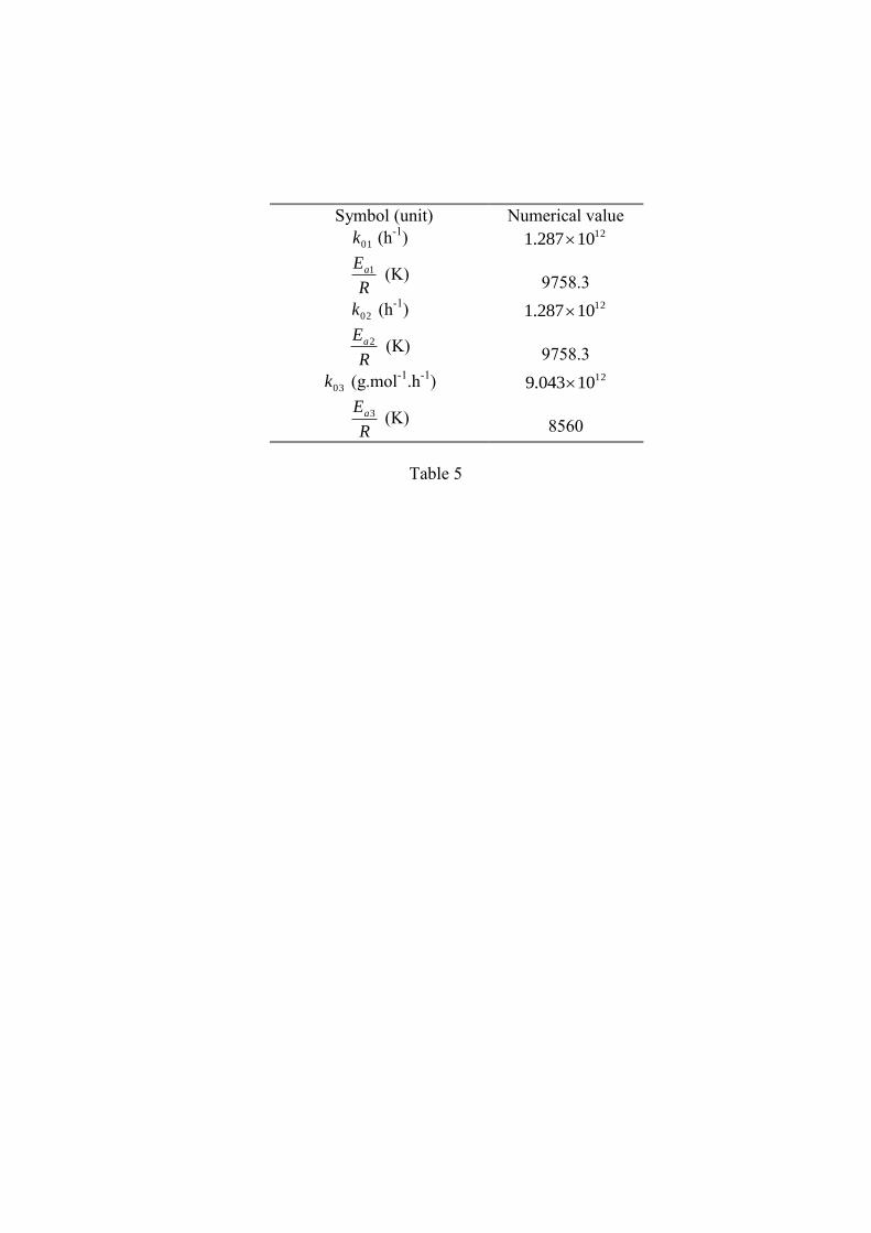
Symbol (unit) Numerical value

01k (h-1

) 1210287.1

R

Ea1 (K)

9758.3

02k (h-1

) 1210287.1

R

Ea2 (K)

9758.3

03k (g.mol-1

.h-1

) 1210043.9

R

Ea3 (K)

8560

Table 5

Symbol (unit)

i* (g.cm

-3)

c p,i* (J.mol

-1.K

-1)

hi ,ref

(J.mol-1

) iM (g.mol

-1)

C5H6 (S1) 0.786 115.3 3109.105 66

C5H7OH (S2) 0.95 763.9 3109.235 84

C5H8(OH)2 (S3) 1.235 529.7 3102.500 102

C10H12 (S4) 0.98 321.6 3104.160 132

H2O (S5) 1 75.327 3108.285 18

H2SO4 (S6) 1.84 138.9 310814 98

Table 6

Symbol (unit) Numerical value inT (K) 15.403

wT (K) 397

q (g.h-1

) 31036

1

in 0.1

5

in 0.85

6

in 0.05

M (g) 31010

(J.h-1

.K-1

) 866880

Table 7

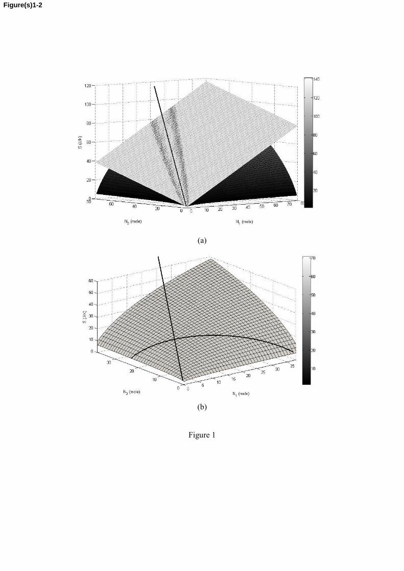
(a)

(b)

Figure 1

Figure(s)1-2

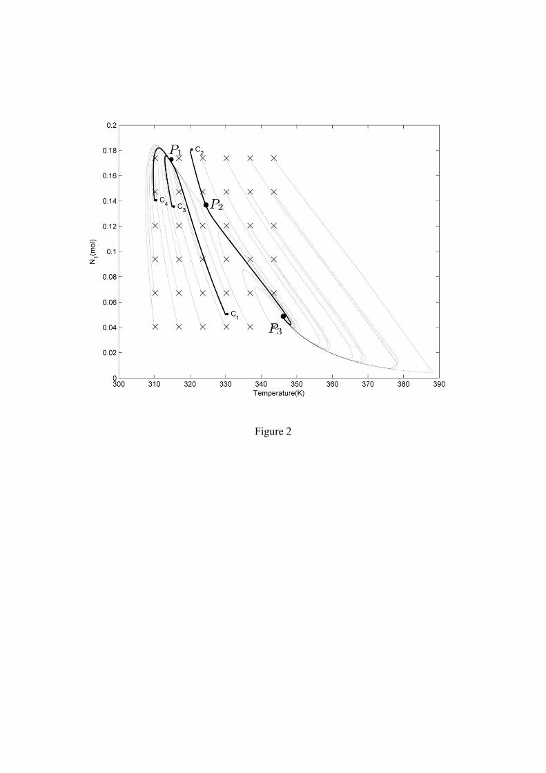
Figure 2

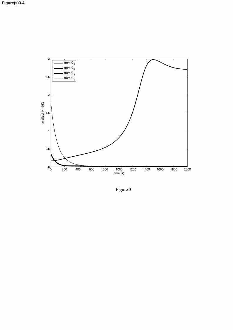
Figure 3

Figure(s)3-4

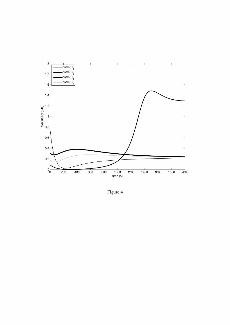
Figure 4

Figure 5

Figure(s)5-6

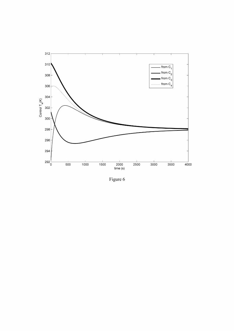
Figure 6

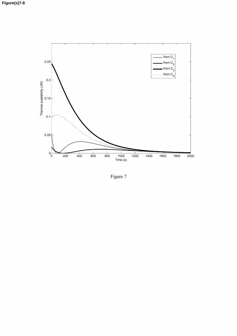
Figure 7

Figure(s)7-8

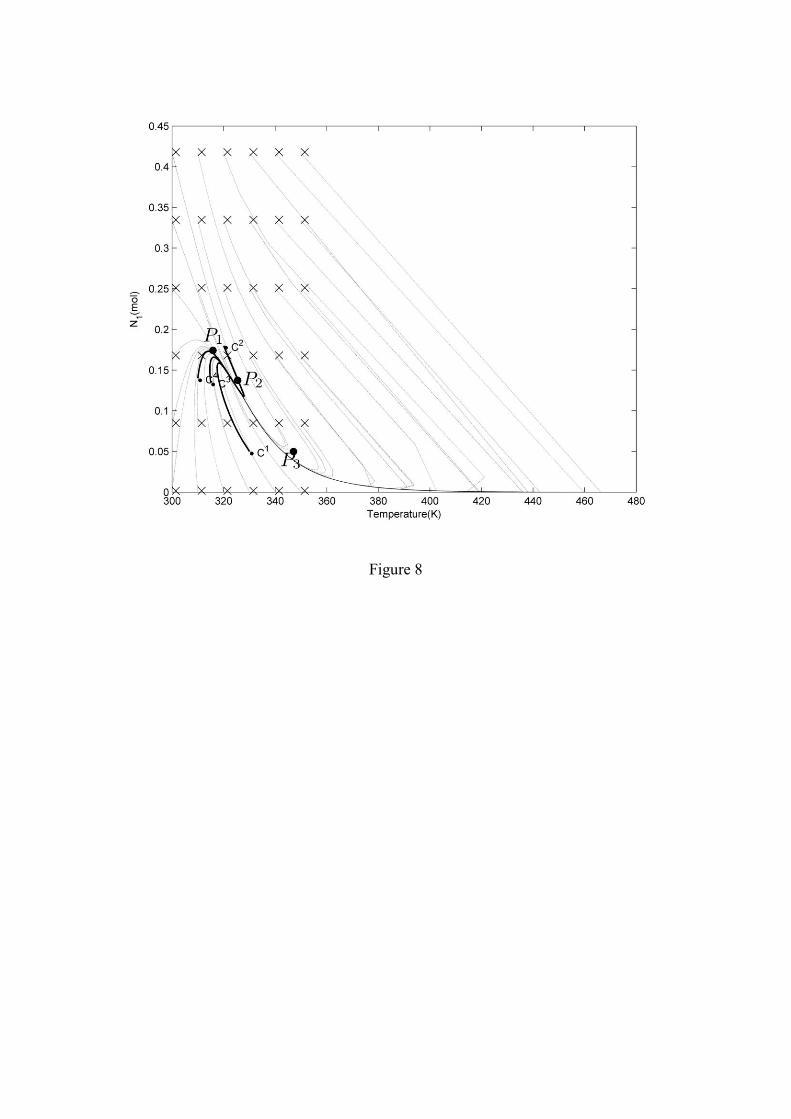
Figure 8

Figure 9

Figure(s)9-to-12

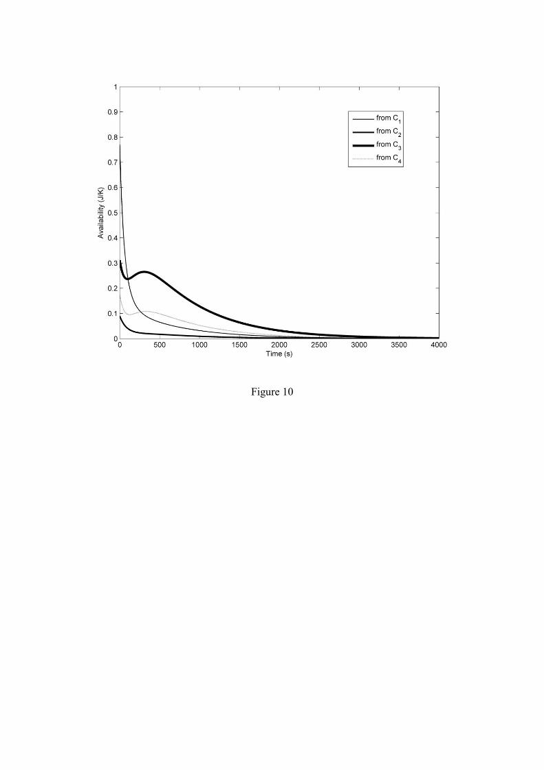
Figure 10

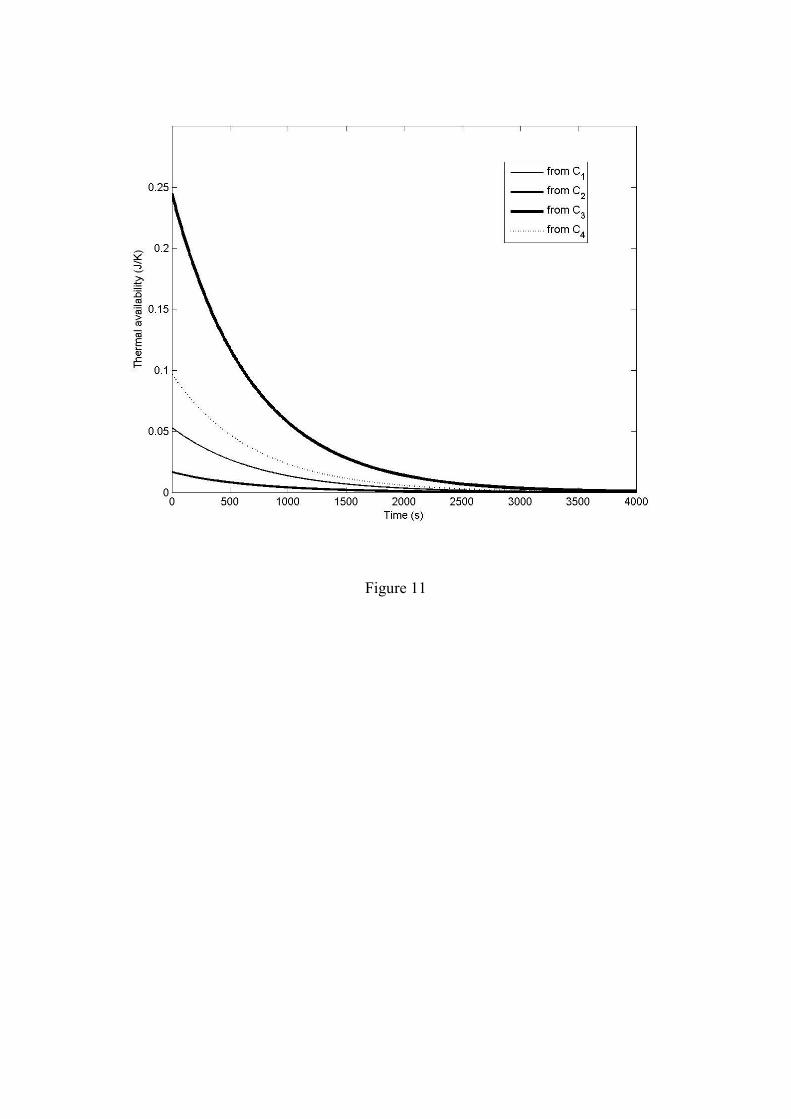
Figure 11

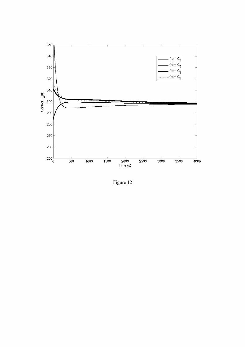
Figure 12

Figure 13

Figure(s)13-to-16

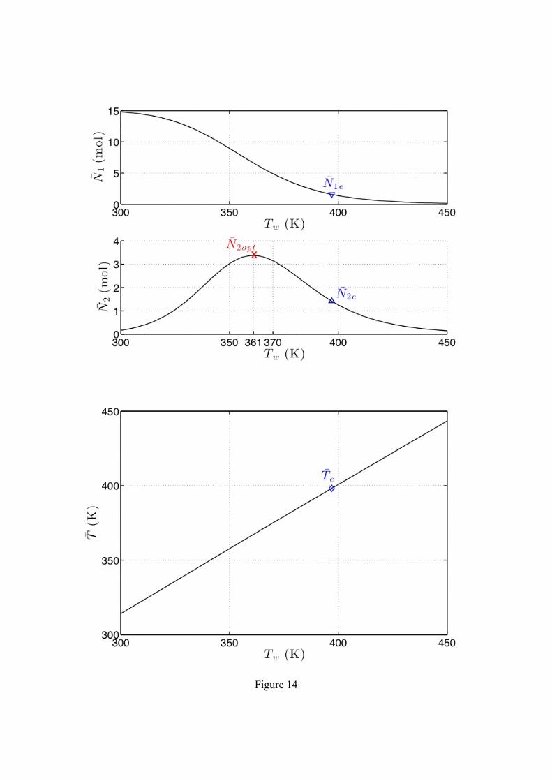
Figure 14

Figure 15

Figure 16

Highlights for

“Thermodynamics based analysis of stability and its use for nonlinear

stabilization of the CSTR” by N. H. Hoang, F. Couenne, C. Jallut, Y. Le Gorrec. submitted to Computers and Chemical Engineering

Highlights > A tutorial description of the thermodynamic availability concept. > Its use for

open loop dynamic analysis of the non-isothermal CSTR. > Its use for Lyapunov based

control laws derivation of the non-isothermal CSTR. > Illustration of the performances of the

controller by simulations. > Comparison of the controller with a proportional one.

Highlights