thermally efficient house final report - welcome to...

Thermally Efficient House

Final Report

Team 5 Brian Barnes

Bhumika Lathia Anupam Pathak Joshua Ravich

ME555 Winter 2005

Abstract In this paper, a description of the progress of a semester project is given. It is our intent to optimize a single livable structure for maximum energy efficiency for the duration of one year. This structure is to be broken down into four sections: the roof with solar panels, a heat pump, doors and windows, and the walls of the structure. Each of these sections will be separately optimized to allow maximum energy efficiency. This optimized efficiency will either be a direct measure of heat, or an indirect but still relevant measure of root-mean-square temperature deviation throughout the year. The intent behind this project is twofold. First, increased heating and cooling efficiency in households would reduce depleting natural resources and consequently reduce the amount of greenhouse and otherwise harmful emissions produced when generating conventional energy used for heating. Second, an increase in efficiency would reduce energy costs, thus creating an economic advantage. We anticipate that our optimized result will produce a structure that would allow a minimum energy requirement over a year, of course obeying physical and practical constraints. Our subsystems are unique enough, that there are sufficient tradeoffs that will be necessary and our constraints will not all be forced to be active. 1.0 Introduction

There are many different engineering and architectural decisions that are needed to be made when designing buildings for varying purposes. The aesthetics, structural soundness, cost, and environmental impact are all aspects which must be considered and possibly optimized. More recently, greater stresses have been put on designing homes to be energy efficient, environmentally friendly, and also economical. In our proposed project for this semester, we plan to respond to this need by optimizing a single room for energy efficiency, while minimizing cost constraints.

Several efforts have been made in the past to create energy-efficient homes, and this field is an active and ongoing area of research and development. Geodesic Domes (Figure 1), for example, originally designed to optimize the volume in an enclosure and were first introduced in the 1950’s as an energy efficient alternative to the traditional house plan (Buckminster-Fuller 2005). However, most furniture is designed to fit against a flat wall (instead of a curved surface) and many people found Geodesic Domes both awkward and inconvenient to live in.

Figure 1: Previous attempts to design a energy-efficient homes

Our design, therefore, will be considerate to the practicality of the living space. For example, it will retain flat walls, and will incorporate basic features of a room such as a door and windows. An average sunlight level may be another design constraint, that will dictate window size and orientation given the room’s directional position in relation to the sun. The geographic location of the room along with heating costs will also be treated as a given in our problem.

Initially all of the subsystems in our single room will be designed to minimize either heating loads, or to minimize the Root-mean-square deviation from a room temperature (assuming the outside temperature is fluctuating with time). The latter design objective is similar to minimizing heating/cooling loads because it would require a minimum amount of energy to maintain a desired temperature. Efforts to minimize this, and other measures of comfort levels have been done in other similar optimization studies (Bouchlaghem and Letherman 1990). When our subsystems are to be combined, it is possible to assign a cost function to all of our variables, and then to minimize cost over, for example, a ten year period. Basically this function would maximize the difference between the long term cost savings of adding extra building materials and the initial building cost. Sub-System Design In the following sections, presentations of each sub-system will be given along with initial models, variables, parameters, and constraints. 2.0 Wall Design By Anupam Pathak

In building an energy-efficient structure, it has been suggested that an amount of “thermal mass” be added in order to store solar and ambient energy during the daytime to lessen the heating loads during the night, and to smooth out any “temperature swings” (Scwolsky and Williams 1982). Some term this effect as thermal inertia, but it really is the effect of an added material’s density, volume, and heat capacity. Water, for example, is cheaply and easily obtained, and has a relatively high heat capacity. It also can be placed in containers inside the thickness of a room’s walls as seen in Figure 1.

Figure 1: A sketch of a room’s wall (width w and height b) with water-filled containers inside.

L w

b

s container

Certain trade-offs would be made in designing the number of containers to be placed in the wall, their spacing, and their diameters. Water has roughly 20 times the thermal conductivity of industrial insulating materials, and placing these cylinders occupy volume that would otherwise be used for insulation. However, without any water in the system, there would be very little thermal, which would be useful in stabilizing temperature fluctuations in the room. The placement of the cylinders within the wall is also something to be optimized. As seen in Figure 2, the cylinders would be placed a distance x from the outside wall surface, and insulation would be placed between it and the wall. If the cylinder is placed too far from the outside wall, it would be difficult to heat it during the daytime. However, if it were to be placed too close to the wall, it would lose much of its heat too quickly during the night time.

Figure 2: A sketch top view of a single container inside the wall thickness.

2.1 Nomenclature V volume T temperature t time G thermal conductance h convection heat transfer

coefficient b wall height v width of water container n number of containers k thermal conductivity L room length W room width A surface area max maximum min minimum c specific heat

Greek Symbols ρ density Subscripts a room air b wall height win window dr door floor floor area l length wd width act actual des desired w water inside cylinder ins insulation ∞ ambient air

xTa Twkins

tw

vz

2.2 Modeling 2.2.1 Objective Function For the subsystem, the cost of the wall insulation added to the present value of the heating costs over the period of 20 years will be minimized. The exterior temperature is varied by the function:

desT

)26.0sin(2023 tTdes += (2.1) where time t is in hours and varies from zero to 24 (to account for the cycle of a single day). Objective: minimize Cost ( ) insinspowerdesaa CVdtCTTcPVCost +−= ∫ )(ρ where PV is the present value of the daily power cost found by the integral. Cpower is the cost of energy per joule, Vins is the volume of insulation used in the room, and Cins is the cost of insulation per square meter. Cins is also dependent on the thermal conductivity of the insulation, as higher quality insulation (with lower k-values) tend to be much more expensive. Using several different price quotes for different insulation types, a cost function was constructed from a power curve fit (Figure 3).

y = 13.979x-0.6709

020406080

100120140160180200

0 0.02 0.04 0.06 0.08

K (W/mK)

Pric

e ($

/m3 )

Figure 3: Cost function for insulating material that will be placed in the room walls.

2.2.2 Constraints The following constraints must be made on the room and wall design: Physical Constraints

Description Equation The amount in insulation between the

water and the outside wall must be greater than or equal to zero.

0≥x

The water thickness must be greater than or equal to zero.

0≥z

The insulation between the water and outside air, the water thickness, and the

insulation between the water and inside air must equal the wall thickness.

wins ttzx =++

The total surface area of the room features (water plus windows and doors) must be

less than or equal the total surface available in the room.

0)(2)( ≤+−++ WbLbWLWLvbn drdrwinwin

The thickness of the water multiplied by the number of containers must be greater

than or equal to zero.

0≥vn

Practical Constraints

Description Equation The surface area of the floor must be

greater than or equal to a minimum area. 0max ≤− floorLW

The length of the floor must be greater than a minimum value.

0min ≤− Ll

The width of the floor must be greater than a minimum value.

0min ≤−Wwd

The thermal conductivity of the wall insulation must lie within an acceptable

range.

001.008.0 ≥≥ insk

The overall wall thickness must fall within a practical range.

01.03 ≥≥ wt

The height of the room must be at least 3.5 meters.

5.3≥b

The thickness of insulation between the water panels and the interior wall must be

at least 5 cm.

05.0≥inst

2.2.3 Variables and Parameters Variables The variables in this subsystem are listed below in symbolic form. Descriptions of each of these symbols can be found in the nomenclature section above.

vn ,L,W,x,z, , kinst ins, ,b wtAdditional variables can be added later as needed. Currently there are six variables and five degrees of freedom. Values of x=0.2, z=0.1, tins=0.3, L=4, w=3.5, b=4, and vn=2 satisfy all of the constraints outlined above and this shows that there is at least one feasible solution to the problem. Parameters

Name Typical Value ac 1006 J/kg.K

wc 4186 J/(kg K) h ~50 w/(m2K)

wρ 998.23 kg/m3

aρ 1.29 kg/m3

∞T Ranging from 0 to 40 degrees C (function over time to be determined)

winL 1 m

winW 1 m

drL 2 m

drW 1 m 2.2.4 System Model

The system model can be broken down into two one for the room air, and the other for the water inside the cylinder. For simplicity, the air inside the room will be treated as a lumped-capacitance element, and its energy balance can be written in Equation 2.2. The ambient temperature can be treated as a known function of time in order to calculate seasonal temperature responses (Zaheer-Uddin 1986).

)()( ,, ∞−−−−= TTGTTGdt

dTVc ainsawawa

aaaaρ (2.2)

The conductance for the room air to the water container is described by Equation 2.3: G

)()(

1,1

,

insw

ainsaw

wa

kAt

hAG

+=

−

(2.3)

where is the surface area of the wall under which the container is placed, and is the thickness of insulation between the water container and the interior wall. Both are described by Equations 2.4 and 2.5. The volume of the room is described by Equation 2.6.

wA ainst ,

bvnAw = (2.4) zxtt wains −−=, (2.5) =Lwb (2.6) aV The conductance for the room air to the insulation thickness (appearing in Equation 2.2) is written similarly to Equation 2.3 as:

11

,

)()()(

1−

∞− ++

=hA

kAt

hAG

insinsins

insains

insa (2.7)

where this time the area of the remainder of the wall is used (Equation 2.8), and is treated as a constant.

inst

))22( vnbLbwAins −+= (2.8) Since the thermal mass of the water has a specific heat capacitance, its transient temperature must be modeled similar to the room air (Equation 2.2). Consequently, a similar energy balance is taken about the water:

)()( ,, ∞∞ −−−= TTGTTGdt

dTVc wwwawa

wwwwρ (2.9)

In this case, the volume of the total water placed in the room is used and can be described as follows: zvbnVw = (2.10) The conductance from the room air to water is the same as Equation 2.3. The conductance from the water to the ambient air, however, is a new relationship and is given in Equation 2.11:

)()(

11

,

insinsins

w

kAxhA

G+

=−

∞

∞ (2.11)

Equation 2.8 and Equation 2.2 are two coupled ODE’s, and a solution can be found for

the room temperature given an ambient temperature either numerically or analytically. Validity of Lumped Capacitance

The validity of using the lumped capacitance method can be measured from the Biot number, which is simply the convection heat transfer coefficient (or an equivalent measure) multiplied by the element thickness and divided by the thermal conductivity (DeWitt 1996). The relative error due to using the lumped capacitance can be estimated to be approximately 1/6 the Biot number. Since both the element thickness and the equivalent heat transfer coefficient are variables (the amount of insulation between the water and outside air is a variable) the Biot number also varies. However, picking values that might be “mid-range” in terms of how much the variables can change, it was estimated that there would be a 10% error in calculated temperature variation.

To get a more accurate solution, Equation 2.8 would become a PDE, and the problem would become much more complicated. Therefore, at this point, and for the scope of this optimization procedure the problem will be formulated as an ODE. Increasing the complexity and accuracy can be done later in the semester if desired.

2.3 Subsystem Summary

In this section, an outline of the optimization problem that was outlined above will be given with the constraints summarized in negative null form. Over the course of one year, the design objective will be: Objective: minimize Cost

( ) insinspowerdesaa CVdtCTTcPVCost +−= ∫ )(ρ

where: 0)()( ,, =−+−+ ∞TTGTTGdt

dTVc ainsawawa

aaaaρ

)()( ,, ∞∞ −−−= TTGTTGdt

dTVc wwwawa

wwwwρ

Subject to: G1: 0)(2)( ≤+−++ WbLbWLWLvbn drdrwinwin G2: 0max ≤− floorLW G3: 0min ≤− Ll

G4: 0min ≤−Wwd

G5: 0max ≤− bb G6: 0≥x G7: 0≥z G8: 0≥vn G9: 5.3≥b G10: 05.0≥inst G11/G12: 001.008.0 ≥≥ insk G13/G14: 01.03 ≥≥ wt H1: wins ttzx =++

The function for the ambient temperature is a known function of time, and it can be approximated as a sinusoid. Later, when all the subsections are to be put together the parameters

for window door width and length can be treated as inputs, and the heat generation can also be treated as an input. 2.4 Model Analysis

In order to produce a solution to Equations 2.2 and 2.9, they were symbolically programmed in the Simulink package of MatLAB. A printout of the Simulink module is provided in the appendix of this paper. However, before the optimization was run, some model conditioning was required, and this section will discuss what was done. 2.4.1 Scaling

In order to ease computational effort required to solve the problem outlined above, and since the time scales in this problem are relatively large, time-scaling had to be done. Normally, the units and calculations done in heat transfer problem are listed in seconds, but because the problem outlined above is linear, it is fairly trivial to alter the time scale. It was chosen that the time scales be in hours since the temperature fluctuations of interest would generally not occur at a scale smaller than this (for this particular problem). Therefore, in both Equations 2.2 and 2.9 a factor of 1/(3600) must be multiplied by the time derivative in order to scale the time to hours. In addition, certain variables and constraints were scaled for the SQP algorithm. Cost, for example, was divided by 1000. The thermal conductivity for insulation was multiplied by 1000. Finally, G2 is divided by 100 to ensure that its values are on the same order of magnitude of other variables and constraints. 2.4.2 Objective Function Modification After viewing the solution to the problem, it became apparent that the inside temperature response follows a sinusoidal wave (as a result of the excitation being a sinusoid). This makes sense because the system is linear. Therefore the objective function can be simplified as minimizing the amplitude of the system response. In essence this produces identical results to the minimizing the least squared deviation from room temperature, but it is easier to program (by keeping track of a maximum deviation over the entire system response, and then using this maximum deviation as the value to be minimized). 2.4.3 Monotonicity Analysis Since Equations 2.2 and 2.9 are not explicit functions, and they require numerical time integration, it is difficult to compute a simple monotonicity analysis. However, when examining

Equation 2.2, it can be seen that the time derivative of the room temperature dt

dTa is directly

related to the objective function – namely that the minimization of this time derivative would produce smaller responses to exterior excitations due to . The volume of the room, as described by Equation 2.6 is multiplied directly by the time derivative, so if the interior temperature response were to be minimized, Equation 2.6 would be maximized. Therefore, from MP1, the variables in equation 2.6 must be bounded from above meaning that G2 must be active. In fact, from the results (which will be discussed in the next section) this is the only inequality

∞T

constraint that is active at the optimal point. This constraint deals directly with the calculation of Equation 2.6, which is the volume of the air inside the room. 2.5 Numerical Results

In this section, the numerical results of some preliminary efforts to obtain an optimal solution using the function fmincon will first be discussed. In these initial efforts, cost was not the objective function. Instead, the goal was to minimize the variation of the room temperature response from 23 degrees C over the course of a day. It was assumed that minimizing this variance will minimize the heating load, and thus minimize any future heating costs.

After these initial results were preformed, the cost function was incorporated into the model, and a full analysis of initial building vs. future payback in the form of heat load reduction was done using Optimus. The results from this comprehensive analysis will be presented and discussed in the last part of this section. 2.5.1 Initial Studies using fmincon

In these initial studies, the model was tested for optimality by minimizing the temperature variation from a nominal value of 23 degrees C. Because cost was not a factor in this optimization, the number of variables decreased as there was no tradeoff for them. For example, thermal conductivity of the insulation had to be fixed at a value, because of function would be monotonic with respect to it (the lowest thermal conductivity would produce a most optimal solution). The same was the case for overall wall thickness and room height. The optimal solution was found after 14 iterations, and the values for each of the variables at this optimum are listed in Table 1. Figure 3 shows the response of the inside air temperature, the water temperature in the containers, with respect to the excitation temperature (the outdoor air temperature). It can be seen that the indoor air temperature response is, indeed, minimal when compared with the outdoor temperature cycle.

Figure 4: A plot of the inside air and water temperatures with respect to the outside temperature variation at the

optimal solution. Temperatures (y-axis) are given in degrees C. Time is in hours.

In addition, the maximum inside room temperature deviation from 23o C is listed as Max(Ta). This is the value being minimized (because the response of the inside temperature is to be minimized). Table 1: The optimal solution produced by fmincon. Max(Ta) is the maximum deviation from room temperature for this optimal solution.

Variable Optimum Variable Optimum x 0.2643 W 6.7082 inst 0.0500 L 6.7082 vn 6.5207 Max(Ta) 25.8977 z 0.3857

Upon closer inspection of the results listed in Table 1, it can be seen that the values for W and L show that the inequality constraint G2 is indeed active: 45=LW (2.12) The fact that L and W are equal shows that the length and width of the room are equally important in this optimization. It also shows that a square floor plan (in agreement with the beginning assumption that the room must have walls at right angles to each other) is the optimal shape for the room. This makes sense from the perspective of heat transfer because this shape would minimize the amount of wall surface area encountering heat loss, but at the same time maximize the volume of the interior air, which is important in minimizing the interior temperature response.

The rest of the inequality constraints are not active, and this implies that a certain tradeoff between the rest of the variables. 2.5.2 Parametric Study From the parameters listed in section 2.2.3, the only ones that may be varied are:

∞T , , , , , kwinL winW drL drW ins

since the rest of the parameters are the physical properties of air and water. For the initial study conducted in the section above, was cycled over an amount described by Equation 2.11. This amount can of course be varied, and it would be interesting to see its effect on the results. The window and door dimensions are also parameters that will be supplied by other optimization efforts from another student. k

∞T

ins, the thermal conductivity of the insulating material can also be varied depending on the material. A sensitivity analysis will be conducted for this as well. Ambient Temperature An optimization procedure was run on a “harsher” day, where the same function as Equation 2.11 was provided but its amplitude was changed from 20 to 30 (50% increase). It was expected that the optimal values for all the variables would not change, and this indeed was the case. The maximum interior room temperature change was larger, however, at 4.34 degrees above room temperature. This reflected a 5.6% change. From a design standpoint, this is an excellent result because it shows that if the outside temperature were to increase by such a drastic amount, the interior temperature would not vary change as much. Windows and Doors As mentioned before, values for the windows and doors are to be supplied by another group member. However, to understand their effect on this particular optimization procedure, a sensitivity analysis was performed. First the length and width of the window was increased by 50% and the following results were obtained: Table 2: The optimal solution produced by fmincon for a 50% increase in window length and width. Max(Ta) is the maximum deviation from room temperature for this optimal solution.

Variable Optimum/%Change Variable Optimum/%Changex 0.2637/ 3.3 W 6.7082/0 inst 0.0500/ 0 L 6.7082/0 vn 6.4426/ 1.2 Max(Ta) 25.927/ 0.11 z 0.3863/ 0.15

The door of the room was similarly increased in width and length, by 50%, and almost identical results were obtained as listed in Table 2. This occurred because the door and window areas factor into the equations in the same way. It can be seen that the windows and doors do not make a big difference on the optimized results. However, this is neglecting the heat loss through the windows and doors (which will be calculated and supplied by the other group member). This should make a much bigger difference on the model. Thermal Conductivity of Insulation The choice of insulating material inside the thickness of the room wall can vary based on cost and effectiveness. To test the sensitivity of this choice, the optimization routine was run for a 50% increase in thermal conductivity. This reflects an insulating material that performs 50% worse than the value used previously. Table 3 shows these results and the %Change from the previously used insulating material. Table 3: The optimal solution produced by fmincon for a 50% increase thermal conductivity of insulation. Max(Ta) is the maximum deviation from room temperature for this optimal solution.

Variable Optimum/%Change Variable Optimum/%Changex 0.2556/ 0.22 W 6.7082/0 inst 0.0500/ 0 L 6.7082/0 vn 6.5207/ 0 Max(Ta) 26.233/ 1.3 z 0.3944/ 2.25

It can be seen that the changes in thermal conductivity affect the optimal solution for x, z, and the value of the objective function at the optimal point. However, again changes of as much as 50% in the thermal conductivity does not drastically affect the solution. From this parametric study, the model outlined above is fairly robust, and provides similar solutions for relatively large variations in parameters. 2.5.3 Full Sub-System Analysis After finding an initial optimal solution, and exploring the robustness of the model and of the optimal solution, the system was modified to account for initial building costs, and future heating costs. All of the variables introduced in section 2.3 were applicable to this model, and a full analysis was then performed using Optimus. The system was also fitted to be easily incorporated with other sections of the larger project. For example, the required hourly heat

loads were calculated and sent to a file that would be read by the model developed for the heat pump design. The SQP algorithm was chosen for this overall optimization, and an optimum cost was found after 20 iterations were performed. The values for the variables at the optimum point were as follows: Table 4: The optimal solution produced when using Optimus for a full analysis on initial and future cost minimization.

Variable Optimum Variable Optimum x 0.053 b 3.5 inst 0.05 w 5 vn 19.14 l 5 z 0.59 kins 0.08

twall 0.7 Cost 1387.56 The results listed in Table 4 suggest that the total wall area covered by sections containing water is 17.4%. This is the optimal amount of water that should be contained in the wall interior. The values for the room width, length, and height are all bounded by below at the optimum (G2 is again active, with the room area set for this optimization run at 25 square meters). This makes sense, because a smaller room would be more efficient. It is also of interest that the optimal floor area is a square. The optimal wall thickness, insulation between the inside wall and water, thickness of the water container, and insulation between the water and outside wall were also determined. Figure 5 shows a CAD drawing of the optimal wall cross section with the water container:

Figure 5: A CAD drawing of the optimal wall cross section. The transparent piece represents the water container,

and the other two pieces around it represent insulation. It is seen that the thickness of the container is much larger than the insulation surrounding it. This is probably due to the stabilizing effects the added thermal mass of the water has on the interior room temperature. According to the optimal results 17.4% of the wall must possess a wall cross section shown in Figure 5, and the rest of the wall must have pure insulation (at a thickness of 0.7 meters).

3.0 Roof-mounted Solar Panel Array By Joshua Ravich 3.1 Problem Statement To increase thermal efficiency of the house, solar panels can be employed to collect solar energy and power other subsystems in the house. With that in mind, this section intends to optimize the placement of solar panels upon the roof of the house. By changing the orientation and area covered by the solar panels, more solar energy will be collected. However, solar panels are quite bulky, and therefore a structural analysis of the roof must be undertaken, to make sure that the panels do not lead to a cave in. While more solar panel coverage will increase the amount of energy collected, too much will cause structural failure. The optimal orientation must be found as well. Yet the sun’s incident angle on the panel changes daily and monthly, and therefore must be taken into account when positioning the panels. 3.2 Nomenclature Table 3.1. All symbols used Symbol Units Definition η none Efficiency of solar panel, as determined by manufacturer Lp m Length of roof covered by solar panels Wp m Width of roof covered by solar panels Sc W/m2 Solar constant, flux of solar energy incident on a surface normal to solar rays f(t) none correction factor for earth's orbital eccentricity 0.97≤ f ≤ 1.03

θi(t) radians The sun's altitude angle on a horizontal surface, dependent on time of day and year

θ radians Elevation angle of the solar panels φi(t) radians Solar azimuth East of North φ radians Bearing of the solar panels ρp Kg/m2 Areal density of the solar panels, as defined by the manufacturer tr m Thickness of the roof ρr kg/m3 Volumetric density of the roof Pcr N Buckling load for the wall X none Safety factor on the yield stress σy N/m2 Yield stress for the roofing material g m/s2 Gravity Lr m Roof length, assumed to be equal to LfloorWr m Roof width, assumed to be equal to Wfloor

ρs Kg/m2 Maximum snow load allowed in Ann Arbor area C none Column constraint coefficient A m2 Area of hollow rectangular column E Pa Young’s modulus r m Radius of gyration I m4 Areal moment of inertia Lc m Length of Column (height of walls) tw m Thickness of walls Costp $/m2 Panel Cost per m^2 r+h none Interest rate + inflation rate m years Time period evaluated

3.3 Mathematical Model This section introduces the mathematical model for the subsystem, and goes through the derivations and assumptions used to reach the model. 3.3.1 Objective function The objective function is to maximize the amount of solar energy collected over one year by the solar panels. One year is necessary in order to cover the sun’s entire range of motion. Solar energy collected is a function of the total solar energy incident on the surface of the panels. However, the sun moves east to west daily, and north to south seasonally, which means that the incident angle of the sun on the panel changes. The sun’s angle from a horizontal surface can be described by an altitude angle, θi, and a directional azimuth angle, φi , measured east of north (see Fig. 3.1). The solar panel can be mounted at an elevation angle, θ, and a bearing angle, φ. Through trigonometry, the total incident energy at a point can be found (see Fig. 3.2).

Figure 3.1. Definition of Azimuth and Altitude

source: http://www.heavens-above.com/gloss.asp?term=azimuth

http://www.heavens-above.com/gloss.asp?term=azimuth

Figure 3.2. Incident energy on a solar panel for an altitude of θι

By a similar analysis, we can find the incident angle for a given azimuth. φ here is the angle east of North to the face of the panel. The direction the panel actually faces is φ + π/2. The total energy incident is then [1]:

)sin()sin(GA E ios,p φφθθ −⋅+⋅⋅= i (3.1) Where: Ap = area covered by the panels = Lp*WpGs,o = solar energy = Sc*f (t) The total energy collected by the solar panels is the total incident energy multiplied by the efficiency of the panel, η, a number dependent on the panel’s manufacturer [2]. To maximize the energy collected, we therefore want to minimize the negative energy collected over a year, to keep with negative-null form. The objective function therefore becomes:

( ) ( )[ ]dttttfSWLEMin iicpp∫ −⋅+⋅⋅⋅⋅⋅−= φφθθη )(sin)(sin)( (3.2) f(t) can be calculated from data as a sine wave that has a 365 day period, evaluated at every hour. Amplitude is 0.06, with a center of 1, which yields (Incropera and DeWitt 2002):

⎟⎠⎞

⎜⎝⎛

⋅+=

365242sin06.01)( ttf π (3.3)

Solar Rays

π – θi - θ Panel

θi θ Roof

To model solar altitude and azimuth over the year, sine waves were used to describe daily and yearly motion of the sun. Data from 6/21/2004 and 12/21/2004 for Ann Arbor, MI were used as the minimum and maximum points of the solar model, because they represent the solstices, and realize the largest and smallest altitude, and the largest and smallest ranges in azimuth change. For 6/21, maximum altitude was 71.2°, with azimuth traveling between 42.2 and 317°. At 12/21, maximum altitude was 24.3°, with azimuth traveling between 111.9 and 248.6° [USNO 2004]. To calculate θi(t), we can approximate maximum daily altitude as a sine wave traveling between minimum and maximum measured over the year. Therefore, we have:

( ) ⎟⎠⎞

⎜⎝⎛

⎟⎠⎞

⎜⎝⎛⋅⎟

⎠⎞

⎜⎝⎛ −

+⎟⎠⎞

⎜⎝⎛⋅⎟

⎠⎞

⎜⎝⎛ +

=3652sin

18023.242.71

18022.713.24max tt πππθ (3.4)

For the daily path, a sine wave of 365x24 frequency is used. Because daily altitude always begins at zero and ends at zero, for these calculations, the sine wave describing daily motion is:

( ) ( ) ( )⎟⎠⎞

⎜⎝⎛+=

242sin

2max

2max tttt πθθθ (3.5)

This expands to:

( ) ⎟⎟⎠

⎞⎜⎜⎝

⎛⎟⎠⎞

⎜⎝⎛+⎟⎟

⎠

⎞⎜⎜⎝

⎛⎟⎠⎞

⎜⎝⎛

⋅+=

242sin1

365242sin065.11325.0 ttt πππθ (3.6)

The resulting sine wave is (see Fig. 3.3):

0 50 100 150 200 250 300 350 4000

0.2

0.4

0.6

0.8

1

1.2

1.4

Days

Sol

ar E

leva

tion

(rad)

Figure 3.3. Model of daily solar elevation over a year.

It should be noted here that daily motion is stretched out to keep the sun moving across the sky for 24 hrs. While this should yield twice the actual incident radiation, it keeps the solar motion continuous as a function of time. To account for this, energy can be divided by 2, because the sun is visible approximately only half of the time. A model for azimuth can be similarly derived. The range of azimuth changes daily, and therefore is modeled here as a sine wave moving between maximum and minimum range over the year. For 12/21, amplitude is (248-111.9)/2 = 68°, and for 6/21 is (317-42.2)/2 = 137°:

⎟⎠⎞

⎜⎝⎛

⋅⎟⎠⎞

⎜⎝⎛

⎟⎠⎞

⎜⎝⎛ −

+⎟⎠⎞

⎜⎝⎛

⎟⎠⎞

⎜⎝⎛ +

=36524

2sin1802

681371802

13768 tAazπππ (3.7)

The average azimuth value is approximately π radians, corresponding to south, which is logical, and can be confirmed by data [USNO 2004]. Therefore, daily azimuth can be modeled as:

( ) ⎟⎠⎞

⎜⎝⎛+=

242sin tAt asππφ (3.8)

Which then expands to:

( ) ⎥⎦

⎤⎢⎣

⎡⎟⎠⎞

⎜⎝⎛

⎟⎟⎠

⎞⎜⎜⎝

⎛⎟⎠⎞

⎜⎝⎛

⋅++=

242sin

365242sin192.0569.01 ttt πππφ (3.9)

The resulting sine wave is (see Fig. 3.4):

0 50 100 150 200 250 300 350 4000

1

2

3

4

5

6

Days

Sol

ar A

zim

uth

(rad)

Figure 3.4. Model of daily solar azimuth over a year.

Because sun does not directly strike the panel if altitude or azimuth is too low, the solar function m-file disregards these points. Additionally, φ here is the angle from north to the panel’s side. The cardinal direction to point the panel is φ + π/2 radians. Because of pure geometric relations, each panel will block some of the light behind it, a function dependent of the panel angle and the solar elevation (see Fig. 3.5).

Solar rays

θi

Figure 3.5 The blocking effect of leading panels.

Only the first panel receives the full amount of sunlight. Subsequent panels receive light over Leff, as seen above. For simplicity, length of a panel is assumed to be 1m. There is no overlap of panels along the roof, therefore the number of panels that can be placed on the roof is Lp/cos(θ), which can be a fraction. That panels really can’t be fractions of panels is ignored to keep calculations simpler. By geometry, Leff can be calculated to be:

( ) ( )( )θθ

θθ+

⋅−=

i

ieffL

sinsincos

1 (3.10)

Therefore, the new objective function is:

( ) ( )( ) ( ) ⎥⎥⎦

⎤

⎢⎢⎣

⎡⎟⎟⎠

⎞⎜⎜⎝

⎛⎟⎟⎠

⎞⎜⎜⎝

⎛−⋅+⋅−⋅+⋅⋅⋅⋅−= ∫ dt

LLtttfSWEMin p

effiicp 1cos

1)(sin)(sin)(θ

φφθθη (3.11)

To combine the subsystems, the common objective function became minimizing cost over a time period. Total cost over this period was determined by NPV analysis. For the solar system, cost is equal to the initial panel investment minus the present value of the cost of electricity saved over the time period. To calculate the cost of electricity saved, DTE rates were used (DTE Energy). Half of the electricity collected by the panels over a year was assumed to be saved at peak hour rates, and half at non-peak hour rates, plus a variable service charge. Inflation could

L =1

θ

Lcos(θ)

Leff Panel 1

θ

Panel 2

be taken into account to raise DTE rates over the years, however, NPV analysis would already account for this, leaving the present value of the rates unchanged. To be safer though, an assumed inflation rate of 3% was added to an assumed interest rate of 5%, to reduce the PV of electricity saved. It should also be noted that any electricity saved past the required amount was assumed to be either stored or sold back at DTE rates. The money saved in a year, in dollars, is then:

3600100000804.0$

36001000203.0$

3600100022.0$

cos ⋅⋅

+⋅⋅⋅

+⋅⋅⋅

=EEEE t (3.12)

NPV for the total period is then given by:

( ) ( )θcos111cos p

ppmt L

WCosthrhr

ENPV ⋅⋅−⎟⎟

⎠

⎞⎜⎜⎝

⎛

++−⋅

+= (3.13)

Which becomes the new subsystem objective function. 3.3.2 Constraints This objective function is subject to a few different types of constraints and assumptions. The first set of constraints includes practical constraints on geometry. The roof used here is assumed to be flat and rectangular. The panels are assumed to be standard panel sizes, however can be stacked behind each other. Because it is not feasible to have one giant solar panel covering the panel area, a cluster of panels covering the same area is assumed to have equivalent performance. The panels are assumed not to cast shadows over other panels, and the house’s orientation, φ, is assumed not to be determined yet, allowing the panels to be aligned with a dimension of the roof. The equivalence assumption is a large assumption, however greatly simplifies calculations. The geometric constraints on the system are direct constraints on the design variables, maximum and minimum bounds for their values. This implies interior optima will exist, however it can be seen that θ and φ are not monotonic because they are sinusoidal, and therefore an interior optimum is not inadmissible. The first two constraints keep Lp and Wp from exceeding the roof dimensions, determined in the floor and walls model:

G1: Lp - Lr ≤ 0 (3.14)

G2: Wp – Wr ≤ 0 (3.15) The next two constraints are on the orientation angles of the panels. For a hemispherical coordinate system we must constrain the elevation and bearing of the panels.

G3: θ − π/2 ≤ 0 (3.16)

G4: φ - 2π ≤ 0 (3.17)

The next two constraints are physical constraints concerning the structural stability of the roof, when loaded with panels. We must first ensure that the panel weight does not cause the walls of the house to buckle. The walls of the house are modeled as a short, hollow rectangular column with fixed ends (see Fig. 3.6). The total weight of the roof is assumed to be evenly distributed across the top of the column. Rankine’s equation for failure due to elastic instability is given below, with C = 4 for a fixed end column (Young 2002).

( )2

2 ,min1 ⎟

⎟⎠

⎞⎜⎜⎝

⎛+

⋅=

yx

y

y

rrLc

EC

AP

πσ

σ (3.18a)

Where:

( )( )wrwrrr tWtLWLA −−−= (3.18b)

And AIr = (3.18c)

Lr

Figure 3.6 Hollow Rectangular Column

Therefore, total weight must not exceed P, as described by (3.18a). Total weight loaded on the roof is determined below. Three loads must be considered. First is the roof weight. This weight is simply the density of the roof multiplied by the volume of the roof. The second load is the snow load. Because this house is designed for the Ann Arbor area, it must meet the snow load requirement for this region, approximately 25 psf (see Fig. 3.7) (mich.gov).

tw

Wr

Fig. 3.7 Snow Load map for residential areas in Michigan

Source: Michigan government. www.michigan.gov/documents/cis_bcc_snow_40405_7.pdf The third load is the solar panel load. Panels are loaded symmetrically from the long ends and from the longitudinal axis (see Fig. 3.8)

Panel Loading

tr

Figure 3.8 Loading profile from solar panels

Assuming even distribution across the walls of the house, total load must be less than the critical load:

G5: ( ) ( ) 0cos

≤−++ crsrrrrppp PtLgW

LgWρρ

θρ

(3.19)

Where cos(θ) accounts for the added weight of the angled panel. The next constraint is based on yield stress analysis. We want:

yX σσ ≤⋅ max (3.20) where X is a safety factor and σy is yield stress. To calculate the stress of the roof, the roof was modeled as a rectangular plate simply supported on all sides. The equation for maximum stress of a plate under center loading is given by (see Fig. 3.9):

Lr

Panel Loading

.5Lp .5Lp

211

maxrtbqa

βσ = (3.21)

Where: q is the applied load (N/m2) and β is interpolated from numerical tables by matlab code (Young 2002)

Lr

Figure 3.9 Center Loading profile By superposition, stress can be calculated by subtracting a center area of a1b1 = (Lr – Lp)Wp from a center area of a1b1 = LrWp. Self-loading and snow load can be determined from the equation:

2

2

maxr

r

tqW

βσ = (3.22)

Where β is found from numerical tables (Young 2002). This leads to the constraint:

G6: ( ) ( )

( )( ) 0coscos

2

2

2

1

2

23 ≤−

⎟⎟⎟⎟⎟

⎠

⎞

⎜⎜⎜⎜⎜

⎝

⎛ −

−++⋅

⋅ yr

ppr

p

r

pr

p

r

rsrr

t

WLL

t

WL

tWt

X σθρβ

θρβ

ρρβ (3.23)

A next step will be to determine stress from a finite element package and link it to the optimization model.

a1

Wrb1

The design variables used cannot take negative values. θ and φ would have meaning if they were negative, but are not necessary by the coordinate system defined. Also, it can be noted that there is a redundancy in the range now given to φ, namely φ = 0 is the same as φ = 2π. This only affects the model in that it can list two different numbers for an optimal φ, which is fine, because they both represent the same angle. Non-negativity:

G7: θ ≥ 0 (3.24a)

G8: φ ≥ 0 (3.24b)

G9: Lp ≥ 0 (3.24c)

G10: Wp ≥ 0 (3.24d) 5.3.3 Design Variables and Parameters There are four design variables used in the objective function. The first is Lp, the length from the edges of the roof covered by solar panels. Lp/2 is covered on each side. Lp is constrained by upper and lower bounds, and the two physical constraints. Wp is the width of the roof covered by solar panels. Wp/2 extends each way across the width from the centerline of the beam’s long axis. θ is the elevation angle of the solar panels, which affects the amount of solar energy incident on the panels. θ appears not only in upper and lower bounds, but also in the physical constraints, because a greater θ leads to more weight distributed over length Lp. The last variable is φ, the bearing angle of the panels, which has upper and lower bounds. Because the sun moves throughout day and year, the optimum stationary angle must be determined through integration of energy received over a year. There are six main parameters used here. The first is the buckling load, Pcr. This is a parameter that changes with wall design, and therefore is dependent on the wall and floor subsystem. The second parameter is σy, the yield stress for the roof material. Based on material selection, yield stress will change. The third parameter is X, a safety factor that can be changed as needed. The last three parameters are the roof dimensions, Lr, Wr, and tr. The length and width parameters are also determined by the floor and wall system, because the roof dimensions are

assumed to be that of the floor dimensions. The thickness can be varied as seen fit, but should be set by roofing standards. As there are four design variables, and no equality constraints, the total degrees of freedom present are 4. 3.4 System Summary This subsystem models and formulates an optimization problem for a solar panel array on a roof. The objective is to maximize the amount of solar energy collected over a year, subject to physical structural constraints and practical geometric constraints. The system can be formulated into negative null form, and appears as follows:

( ) ( )⎥⎥⎦

⎤

⎢⎢⎣

⎡⋅⋅−⎟⎟

⎠

⎞⎜⎜⎝

⎛

++−⋅

+=−

θcos111cos p

ppmt L

WCosthrhr

ENPVMin

Subject to: G1: Lp - Lr ≤ 0 G2: Wp – Wr ≤ 0 G3: θ − π/2 ≤ 0

G4: φ - 2π ≤ 0

G5: ( ) ( ) 0cos

≤−++ crsrrrrppp PtLgW

LgWρρ

θρ

G6: ( ) ( )

( )( ) 0coscos

2

2

2

1

2

23 ≤−

⎟⎟⎟⎟⎟

⎠

⎞

⎜⎜⎜⎜⎜

⎝

⎛ −

−++⋅

⋅ yr

ppr

p

r

pr

p

r

rsrr

t

WLL

t

WL

tWt

X σθρβ

θρβ

ρρβ

G7: -θ ≤ 0 G8: -φ ≤ 0 G9: -Lp ≤ 0 G10: -Wp ≤ 0

3.5 Model Analysis Monotononicty analysis results in the following table: Table 5.2 Monotonicity Table θ φ Lp Wp

f ? ? ? ? g1 + g2 + g3 + g4 + g5 + + + g6 + + + g7 - g8 - g9 - g10 -

It is unknown if θ and φ are monotonic. They affect the objective function by sin(θi(t)+θ), and similarly for φ, so their effect depends on θi(t) and φi(t). For φi + φ< π/2, f is monotonic decreasing with respect to those two variables, but if φi + φ is greater than π/2 radians, f will increase monotonically with φ. Yet, it can be seen that the term Lp/cos(θ) appears in the objective function. The 1/cos(θ) term decreases as θ increases, which is the opposite of the sin(θ + θi) term. Therefore, we are not quite sure the effect of θ or φ. However this is not particularly important, as it is expected that θ and φ will correspond to an interior optimum with respect to those variables. With this updated model is also possible that θ will be bounded by g5 or g6, as weight increases with θ. It is unknown in this new model whether or not f is monotonic with respect to Lp and Wp. Increased paneling increases the energy collected, and thus the money saved, but also increases cost, leaving it difficult to ascertain the nature of the function. 3.6 Numerical Results Below is a table of constants values used for the Solar panel model in the solution to be presented (see Table 3.3). Table 3.3. Solar panel model constant values Symbol Value Unit g 9.81 m/s^2 ρr 800 kg/m^3 plywood ρp 22.02 kg/m^2 panel ρs 122.3 kg/m^2 snow

allowed

Sc 1353 W/m^2 E 6.90E+09 Pa Plywood* σy 1.38E+07 Pa Plywood** η 0.12 none efficiency r+h 0.05+0.03 none rates Costp 130.75 $/m^2 panel m 20 years ytd

*source: www.answers.com/topic/young-s-modulus**source: http://homepages.which.net/~paul.hills/Materials/MaterialsBody.html For the progress report, parametric studies were performed on the effect of roof thickness. A summary of the results appears below (see Fig 3.9(a)-(c)).

0

20

40

60

80

100

120

140

160

0.5 0.4 0.3 0.2 0.195 0.19

Roof Thickness, tr [m]

Pane

l Are

a Lp

*Wp

[m^2

]

Figure 3.9(a) LpWp vs tr

0

10

20

30

40

50

60

70

80

90

0.5 0.4 0.3 0.2 0.195 0.19


Pane

l ele

vatio

n an

gle

, the

ta [d

eg]

Figure 3.9(b) θ vs tr

http://www.answers.com/topic/young-s-modulus

http://homepages.which.net/~paul.hills/Materials/MaterialsBody.html

0.00E+00

5.00E+08

1.00E+09

1.50E+09

2.00E+09

2.50E+09

3.00E+09

3.50E+09

0.5 0.4 0.3 0.2 0.195 0.19


Ene

rgy,

E [J

]

Figure 3.9(c) E vs tr

From these plots it can be seen that as roof thickness decreases, maximum attainable energy decreases. Because stress increases as thickness decreases, elevation angle must decrease to reduce load, lowering away from an unconstrained optimum. Likewise panel area must decrease. The second parametric study was performed on Lr/Wr, the ratio of the roof dimensions. This parameter was observed at 1.0, 1.4, and 2.0, for roof thickness 0.195m. For a value of 2, there was no feasible solution, because bending stress from the snow load was too great. However, it can be seen that the solutions were fairly similar for 1 and 1.4. Even Lp for 1.4 was close to Lp for 1.0. The results can be seen below (see Table 5.5). It can be seen that because of g1 and g6, the 1.4 test allowed elevation angle and length covered by the panels to be slightly greater than the 1.0 case.

4.0 Windows and Doors Design By Bhumika Lathia 4.1 Introduction Windows are a vital part of any home—they allow natural light into the home providing views and fresh air. Well-planned and protected windows improve comfort year-round and reduce the need for heating in winter and cooling in summer. Doors are the means of ingress and egress for the person inside the home/room. Fenestration refers to any aperture in a building envelope. Fenestration components include glazing material, either glass or plastic; framing, mullions, muntins, dividers, opaque door slabs; external shading devices; internal shading devices; integral (between-glass) shading systems. Fenestration can serve as a physical and/or visual connection to the outdoors, as well as a means to admit solar radiation. The solar radiation provides natural lighting, referred to as day lighting, and heat gain to a space. Fenestration can be fixed or operable, and operable units can allow natural ventilation to a space and egress in low-rise buildings. Fenestration affects building energy use through four basic mechanisms—thermal heat transfer, solar heat gain, air leakage, and day lighting. The energy impacts of fenestration can be minimized by (1) using daylight to offset lighting requirements, (2) using appropriate glazings and shading strategies to control solar heat gain to supplement heating through passive solar gain and minimize cooling requirements, (3) using appropriate glazing to minimize conductive heat loss, and (4) specifying low air leakage fenestration products. A designer should consider architectural requirements, thermal performance, economic criteria, and human comfort when selecting fenestration. Determining Fenestration Energy Flow Calculating a residential heating load involves estimating the maximum (block) heat loss of each room or space to be heated and the simultaneous maximum (block) heat loss for the building, while maintaining a selected indoor air temperature during periods of design outdoor weather conditions. Heat losses are mainly • Transmission losses or heat transferred through the confining walls, glass, ceiling, floor, or other surfaces • Infiltration losses or energy required to warm outdoor air leaking in through cracks and crevices around doors and windows, through open doors and windows, and through porous building materials

Unprotected glass and winter discomfort The transmission heat loss and heat gain from doors and windows during winter and summer seasons respectively play an important role in adding the heating or cooling load on the unit. So our objective will be to minimize this load while providing sufficient natural lighting as well as some portion of the heating during the winter. This leads to a trade off between the area of glass and thus the number of windows provided in a building and heating or cooling load gain. So we want to optimize the heating or cooling load gain of a room taking into consideration the load due to heat transfer from doors and windows. We will also consider the heat transfer due to the infiltration of air which occurs due to the cracks in windows and is mainly driven by the pressure difference. The orientation of the window plays a very important role in reducing the load on the heating/cooling equipment. This will be taken into account when considering the total heat transfer.

Greek Symbols Nomenclature c specific heat ρ density V volume ∆ Difference T temperature ω Humidity Ratio t time h convection heat transfer coefficient Subscripts k thermal conductivity a room air b height b wall height L length win window W width dr door A area floor floor area max maximum l lenth min minimum q Volumetric flow of outdoor air entering

wd width ins insulation

the building in litre/second ∞ ambient air E Incident total irradiance Q Load

out Outside condition in Inside conditions

I Infiltration o over all U heat transfer coefficient pf Projected area of fenestration hfg Latent Heat of vapour t total SHGF Solar Heat gain Factor f fenestration SC Shading Co efficient des desired frame frame glass glass 4.2 Modeling Objective Function Minimize the cost of installing the doors and windows subject to space and energy constraints. This Load is the sum of the Heat gain due to heat transfer from Doors, windows, and heat gained/lost due to infiltration which includes the sensible and latent heat gain/lost. Minimize D D=∑Total Cost Constraints: The following constraints are there on the window and door design Description Equation Width of the Door must be less than wall width Wdr<Wwall

Width of the window must be less than wall width Wwin<WwallWidth of the Door greater than or equal to minimum door width Wdr>= WmindrHeight of the door is less than 0.75 times the height of the wall bdr<0.75bwallHeight of door is greater than or equal to minimum height of door bdr>=bmindrArea of the fenestration i.e.glass is less than or equal to 25% of floor area Af<=0.25AfloorInfiltration is less than 2.5litre per second per square metre of fenestration area

I*Af<2.5

Length of the door is greater than the minimum length Ldr >= LmindrLength of the door is less than the maximum available length Ldr<=LmaxdrLength of the window is less than 10% of the room length Lwin <=0.1 LminwinArea of the glass is greater than or equal to 5% of window 0.8*Awin <=AglassOverall area of the window is positive -Ao<0 Length of window is greater than 8 times its width Lwin >= 0.8WwinLength of door is greater than 8 times its width Ldr >= 0.8WdrWidth of each glass is greater than minimum width w>wmin Width of each glass is less than maximum width w<wmax Variables The variables in this subsystem are Length of door(Ldr),Width of door(Wdr),Height of door(bdr), Length of window(Lwin),Width of each glass (w),Height of window(bwin). Each of these variables are well constrained by the above mentioned constraints. Parameter Name Typical Value ho 29 W/m2k hi 8.29 W/m2k Kdoor 0.035 W/mk Kglass 1.3 W/mk cair 1KJ/kgk ρair 1.2 kg/m3

hfg 2500KJ/kg Uframe 3.5W/m2k Lroom 10 m Wroom 8 m broom 5 m No. of air changes/hr 0.5 Wwall 0.3 m SC 0.8

Resistance of air films and glass to heat flow

System Model The cost of installing the doors and windows is calculated using the data obtained from the net regarding the price of doors and windows.

The data is collected of the window price per sq metre area based on thickness and door price per square meter area based on thickness and then a line statistic is plotted to get the equation in excel The graph for those look as follows: For window

Price of window per meter square for a given thickness

0.005

0.01

0.015

0.02

0.025

0.03

30 35 40 45 50 55 60 65 70

Price

Thic

knes

s in

met

re

price of window per sq mLinear (price of window per sq m)

The equation for cost obtained per sq metre based on thickness is Cwin=2047*wwin+17.5 Now this cost is multiplied by the area of the window to get the total cost of the window Wintotal=cwin*lwin*bwin For the door: The equation for cost obtained per sq metre based on thickness is Cdoor=187.37*wdr+39.33 Now this cost is multiplied by the area of the door to get the total cost of the door doortotal=cdoor*ldr*bdr

Price of door per sq m

-0.02

0

0.02

0.04

0.06

0.08

0.1

0.12

0.14

0.16

0.18

30 35 40 45 50 55 60 65 70

price

thic

knes

s

price of door per sq metreLinear (price of door per sq metre)

Now this cost is minimized to get the optimum area of doors and windows. Based on the length and width of the doors and window, the total load per hour is found and given to the model for the heat pump We divide the load on the system as heat transfer load and infiltration load. Heat transfer load is calculated as follows: Transmission loss from doors and windows can be done using the basic equation of heat transfer For windows we have: Qwin = (Uo*Ao*(Tout-Tin)+Ao*SHGF*SC)/1000

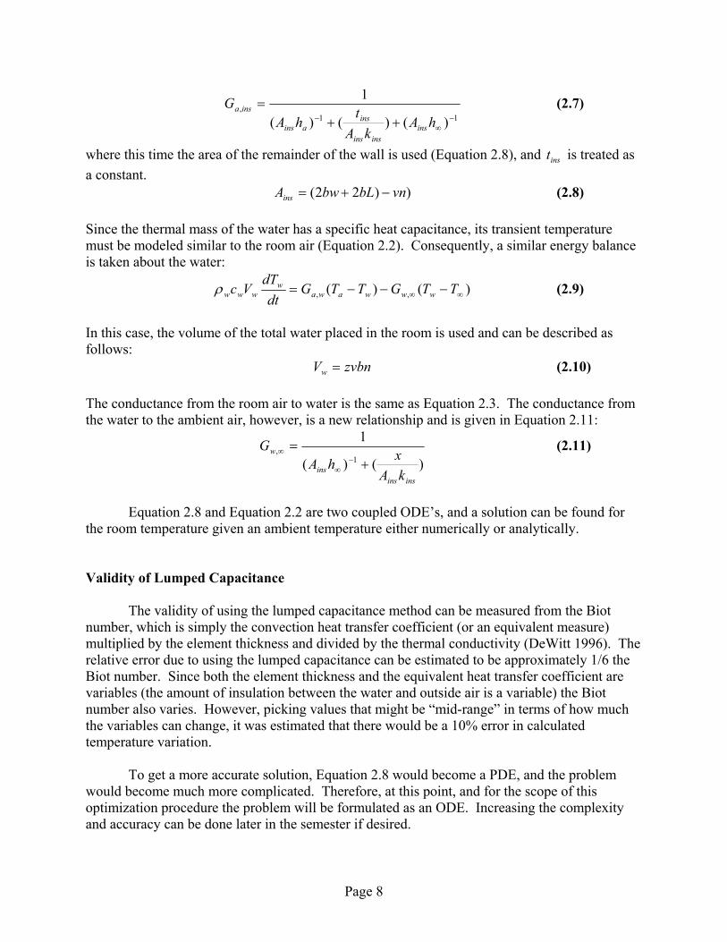
where Qwin is in KW Here Tin is assumed to be fixed at 23ºC Tout is a function of time in hrs which is found to be Tout=(20*sin(0.26*t)+23 Here t is the time in hrs.

Temperature(Function of time in hrs) in degree Celcius

0

5

10

15

20

25

30

35

40

45

0 5 10 15 20 25

Time in hrs

Out

side

Tem

p (D

egre

e C

elci

us)

Temperature(Function of time in hrs) indegree Celcius

Here the heat transfer coefficient for glass windows is is

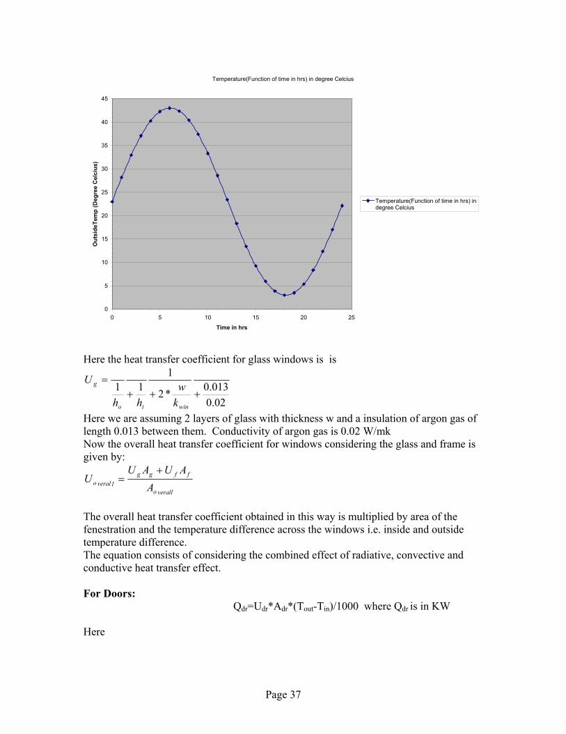
02.0013.0*2

111

+++=

winio

g

kw

hh

U

Here we are assuming 2 layers of glass with thickness w and a insulation of argon gas of length 0.013 between them. Conductivity of argon gas is 0.02 W/mk Now the overall heat transfer coefficient for windows considering the glass and frame is given by:

verallo

ffgglveralo A

AUAUU

+=

The overall heat transfer coefficient obtained in this way is multiplied by area of the fenestration and the temperature difference across the windows i.e. inside and outside temperature difference. The equation consists of considering the combined effect of radiative, convective and conductive heat transfer effect. For Doors: Qdr=Udr*Adr*(Tout-Tin)/1000 where Qdr is in KW Here

drdr W

kU =

Assuming that the door is made of wood slab i.e. homogenous composition and Wdr is the thickness of the door. Infiltration heat loss: Sensible Heat Loss: Energy required to warm/cold outdoor air entering by infiltration to the temperature of the room is given by Qsensible=c*q*ρ*(Tout-Tin) After substituting the values of the parameters c and ρ we have Qsensible=1.2*q*(Tout-Tin) KW Here q is the volume flow rate of the outdoor air entering the building in litre/second

3600*1000changes/hrair of No*b*W*L roomroomroom=q

Assuming medium air tightness, for a given temperature the no of air changes can be found from Table 7 chapter 27 ASHRAE Fundamentals Handbook. Latent Heat Loss: When moisture must be added/removed to/from the indoor air to maintain comfort conditions the energy required to evaporate/add water lost by infiltration gives rise to the latent heat loss

1000h*)- *q

Q fgoilatent

ωωρ (∗=

Substituting the values of parameters we have, Qlatent=3*q*( ωi- ωo) KW The humidity ratio ωi and ωo may be given or can be found from given temperature, Relative humidity(φ) and corresponding saturation pressure(Ps) using basic Psychometry equations like

s

v

PP

=φ

vt

v

PPP

−=

*622.0ω

Different values of ω were found at different temperatures and humidity and a line statistic is plotted through them to get the following equation for Humidity ratio ω. ω = (0.000265* Tout)+(0.000873*RH)-0.02443 Assuming RH of 60% we find the various values of ω corresponding to Tout is plotted

Humidity ratio(function of time)

0.025

0.027

0.029

0.031

0.033

0.035

0.037

0.039

0.041

0 5 10 15 20 25

Time(hrs)

Hum

idity

ratio

(kg/

kg o

f d.a

)

Humidity ratio(function of time)

Thus the total heat gain/lost is given as follows Qt=Qwin+Qdr+Qsensible+Qlatent Thus the whole model looks like: Objective: Minimize Total Cost(Ldr, Wdr, bdr, Lwin, w, bwin,) Subject to: G1: Wdr - Wwall <0 G2: Wwin - Wwall <0 G3: Wmindr - Wdr<=0 G4: bdr- (0.75 broom)<=0 G5: bwin - 0.75bdr <0 G6: bmindr - bdr<=0 G7: Af - 0.25Afloor <=0 G8: I*Af - 2.5 <0 G9: 0.8- Ldr <=0 G10: Ldr - 2<=0 G11: Lwin - 0.1* Lroom <=0

G12: - Ao <=0 G13: ((0.8* Lwin* Wwin)- Af<=0 G14: 8*Wwin - Lwin <=0 G15: 8*Wdr - Ldr <=0 G16: - Aglass <=0 G17: (0.008-w)<=0 G18:w-0.03 <=0 Formulas: Cwin=2047*wwin+17.5 Wintotal=cwin*lwin*bwin Cdoor=187.37*wdr+39.33 doortotal=cdoor*ldr*bdr Total Cost = Wintotal+doortotal Tout=(20*sin(0.26*t)+23 ω = (0.000265* Tout)+(0.000873*RH)-0.02443 Qwin = (Uo*Ao*(Tout-Tin)+Ao*SHGF*SC)/1000

02.0013.0*2

111

+++=

winio

g

kw

hh

U

verallo

ffgglveralo A

AUAUU

+=

Qdr=(Udr*Adr*(Tout-Tin))/1000

drdr W

kU =

Qsensible=1.2*q*(Tout-Tin)

10003600*changes/hrair of No*b*W*L roomroomroom=q

Qlatent=3*q*( ωi- ωo)

s

v

PP

=φ

vt

v

PPP

−=

*622.0ω

Qt=Qwin+Qdr+Qsensible+Qlatent Solving the Optimization problem in Optimus, the following results were obtained: parameters t=0:1:24 to=20*sin(0.26*t)+23; ti=23; ACH=0.5; ho=29; hi=8.29; kwin=1.3; lroom=10; wroom=8; broom=5; wwall=0.3; uf=3.5; kdr=0.035; Scaling: Scaling was performed on the variables and output of the model. The goal of scaling was to get nominal values within a single order of magnitude. Variables w, wdr were scaled and accordingly the constraints were scaled and the following result is obtained for the above parametric values Start End Iter 1 10 Mode start Grad Lwin 2 0.56911 W 6 8 Bwin 4 0.58773 Ldr 1 0.8 Wdr 15 10 Bdr 3 2.2 Qtotal 10.4388 0.420941

Totalcost 751.707 127.033 G1 -15 -20 G2 -0.275 -0.271 G3 -10.6 -5.6 G4 -7.5 -15.5 G5 17.5 -10.8227 G6 -8 0 G7 -12.3564 -19.7415 G8 -24.9998 -25 G9 -0.2 0 G10 -1 -1.2 G11 1 -0.43 G12 -12.436 -9.9E-5 G13 -8 -0.323 G14 -1.8 -0.337 G15 2 -0.2580492 G16 -7.6436 -0.25 G17 2 0 G18 -24 -22 Goal 751.707 127.033 From the above spreadsheet it is seen that all the constraints are well satisfied and the problem is well bounded For Sensitivity Analysis the Parameters which are lroom, wroom, broom which depends on other’s data were changed to 13, 10 and 7 respectively and the SQP was run again and the result was 127.04 which says that the system is quite robust. Also the nominal values of lwin, w, bwin, ldr,wdr,bdr were changed to 3,9,5,3,25,4 from 2,6,4,1,15,3 respectively and in this case the cost came to be around 127.557 and the variable values were 0.634891,8,0.5195,0.8,10 and 2.2 respectively. Monotonicity Analysis:

Ldr Wdr bdr Lwin w bwinF + + + + + + G1 + G2 + G3 - G4 + G5 - + G6 - G7 + + G8 + + + +

G9 - G10 + G11 + G12 - - G13 u u G14 - + G15 - + G16 - - G17 - G18 +

From the monotonicity Analysis we find that Ldr, Wdr, bdr, Lwin, Wwin, bwin, Constraint G6 is active with respect to bdr G9 is active with respect to ldr G17 is active with respect to w The system has 3 degrees of freedom Right now the Sensible and Latent heat gain are constant for any change in the variables because they depend on the room volume. So a change will be seen in the sensible and latent heat load when the whole model is put together.

5.0 Ground Coupled Heat Pump (GCHP) By Brian Barnes 5.1 Problem Statement The thermal project room needs an air conditioning system which can heat and cool the interior. Traditional systems use separate components to heat (gas furnace) and cool (electric cooling). Ground coupled heat pumps can perform both heating and cooling using the same equipment. The term “ground coupled” implies the heat pump uses the earth as a source and sink for the energy needed to heat or cool the living space within a home (Jones, Beard et al. 1996). The energy in the earth is the results of stored solar energy transferred to ground through, solar radiation, rain, wind, etc. In most areas the ground temperature below the surface only vary by about ± 20oF during the year which allows for much more efficient operation than standard air-source heat pumps. Cane and Forgas estimate that current North American practice results in ground loop heat exchanger lengths being oversized by about 10% to 30%, demonstrating a strong need for optimization (Cane and Forgas 1991).

While there are many types of heat pumps, there are only two types of ground coupled heat pumps commonly used. Vertical pipe heat pumps, shown in Figure 5. 1, have the water pipes installed in a system of holes drilled into the ground.

Figure 5. 1 Vertical pipe ground coupled heat pump subsystem (Incropera 1996) Horizontal pipe heat pumps, shown in Figure 5.2, have the water pipes installed in trenches on the property. For the thermal project room, a horizontal pipe system will be used. Horizontal pipe systems are more commonly used in residential applications because they are easier to install, monitor, and repair. The horizontal pipes are usually buried within 6ft of the surface and can be easily installed with a contractor’s ditch witch. Vertical heat pumps are often used in commercial buildings, where the water pipe bore

holes are generally found directly under the foundation and installed before the building construction.

Figure 5.2 Horizontal ground coupled heat pump (Ball, Fischer et al. 1983) The most critical design element for ground coupled heat pumps are the ground coil sizing. Increased coil length results in better performance potential, although inefficiencies due to excessive pumping cost due to head loss, and the added excavation expense require limited pipe length. The cyclic ground temperature will also be a source of trade-offs. Ground coils used for cooling are generally buried deeper in the ground to take advantage of the huge heat capacity of the earth. Heating coils are usually found in more shallow depths to take advantage of solar energy recharging the soil (Langley 1989). The first record of the concept of using the ground as a heat source/sink for a heat pump is in a Swiss Patent issued in 1912. However it wasn’t until the late 1940s that major ground coil heat pump projects were undertaken in the United States. These projects were run by an electric utility heat pump committee and the results delivered “no apparent workable design equations” (Ball, Fischer et al. 1983). Between the 40’s and 70’s most of the GCHP research was done in Europe. The OPEC oil crisis in the 70’s caused a renewed interest in GCHP technology in the United States. The first design methodologies widely adapted were “rules-of-thumb” developed by Ball et al in the early 80’s (Ball, Fischer et al. 1983). The rules related the required heat load to standard lengths and pipe dimensions. During the same time Bose’s research at Oklahoma State University established the school as a leader in GHCP research (Bose and Parker 1983). Today, the Building and Environmental Thermal Systems Research Group as OSU has developed software, GLHEPRO, used for designing ground loop heat exchangers for use with ground source heat pump systems, focusing on vertical pipe commercial systems. It is sold by the International Ground Source Heat Pump Association (University 2005). Kavanaugh, an OSU alumni and professor at Alabama St. has published numerous papers and his thesis on analytical modeling of the behavior of vertical GHCPs (Kavanaugh 1985). The American Society of Heating, Refrigerating and Air-Conditioning Engineers (ASHRAE) has published the majority of the paper on GHCP modeling and simulation in their yearly journal. ASHRAE has also developed reference handbooks for standard heating/cooling system design which will be used in this project.

5.2 Nomenclature t Time (hours) g Gravity (m/s^2) Tg Ground temperature (C) z Pipe depth (m) ID Pipe inner diameter (m) OD Pipe outer diameter (m) kp Pipe conductivity (W/m-C) heq Equivalent convection coefficient (W/m2-K) hL Head loss in pipe (m) m Flow rate in pipe (kg/s) Ti Exchanger inlet temperature (C) To Exchanger outlet temperature (C) η Efficiency of heat pump/exchanger λ Roughness of pipe (m) υ Kinematic viscosity of water (m2/s) ρ Density of water (kg/m3

)

pc Specific heat of water (kJ/kg K)

reqQ Required heat rate (W/s) 5.3 Mathematical Model 5.3.1 Objective Function The purpose of a heating/cooling system is to provide the correct amount of heat at the correct time. A building either gains or looses heat at a rate (W) to the environment, as modeled in the other subsystems. Therefore, there is a required heat load as a function of time which must be met by the heat pump system, . The objective of the optimization is to minimize the power consumed by the GHCP system over time. For this model a bin system with hour-by-hour year long simulation will be run. In each hour bin the atmospheric and ground temperature will be assumed constant with respect to time. There will be 8760 hour bins in the year and the objective function will be the minimization of the sum of the differences between the required and generated heat in each bin. The sum is essentially the kW·hrs required to run the water pump for an entire year.

Q

)(tQreq

Pump Power = ρ⋅⋅⋅ ghLm (5.1) Objective: minimize f

(5.2) ρ⋅⋅⋅= ∑=

gft

8760

1

hL(i)(i)m

5.3.2 Constraints Physical Constraints The focus of the GCHP optimization is the layout of the system, not the heat pump/exchanger equipment. Therefore a simplified model of the equipment will be used. The basic equation for calculating heat flow rate based on energy balance in heating systems was found (OSU):

))(( iopreq TTcmQ −= (5.3) This assumes the equipment is 100% efficient. A standard efficiency, η, is introduced to model the system. The value of η = 70% was chosen based on number for standard heat pump/exchanger systems used with GCHPs as stated by Bose (Bose and Parker 1983). The modified system model is:

( )[ ]))(2.4(/1 ioreq TTCkgmQ −= η (5.4) The water flowing through the ground coil pipes encounters flow resistance in the pipe. The amount of resistance in calculated in the head loss. The head loss is a function of the, flow rate, dimensions of the pipe, and the pipe material. An excel model was found which calculates the head loss with given inputs (Sellens 1998). The excel model was transferred to C-Code for the optimization.

),,,,,( ρυλdLmfhL = (5.5) The heat transfer model for fluid flow in a pipe can be found in standard text books. The standard form of the heat transfer equation with TTT g −=∆ (Incropera 1996):

( ) ThcmP

dxTd

eqp

∆=∆

− , where P= perimeter = πD (5.6)

Separating variables and integrating over the length of the pipe:

( )∫

∆

∆−=

∆∆o

i

T

T

L

eqp

dxhcmP

TTd

0∫ (5.7)

Solve this integral equation it is found that

⎟⎟⎠

⎞⎜⎜⎝

⎛−=

−

−eq

pig

og hcm

DLTTTT πexp (5.8)

The heat transfer coefficient must also be calculated for this application. An equation was found for heat transfer coefficient from a liquid through the solid pipe material (Incropera 1996):

Dk

h weq

36.4= (5.9)

Where is the average heat transfer coefficient for water in a pipe assuming fully developed flow. The fully developed flow assumption is valid for L>>d, which is present in the system.

eqh

Practical Constraints The maximum flow rate and allowable head loss are characteristics of the water pump in the system. Standard water pumps in GCHP systems are on the order of 5 HP (Langley 1989). In order to bound these values it was assume the largest allowable water pump will be a 5 HP pump. The pump characteristics for a common water pump were found for the Amos PM81 Economy Pump . The maximum pump performance metrics are:

skg 0.1m ≤ (5.10)

mhL 5≤ (5.11)

The maximum pipe length allowed by the available yard area is shown in Figure 5.3. To insure that heat transfer through the soil does not effect pipes in close proximity a 5 m spacing is assumed. The spacing is also practical for pipe installation; it is difficult for a trenching machine to produce tightly packed trenches. With these assumptions the maximum available pipe length will be:

mL 150≤ (5.12)

Figure 5.3 Pipe layout for project building with maximum pipe length The inner and outer diameters of the pipe to be used should be within the range normally used in GCHP system. Ball states that standard piping has an ID of 1 to 5 cm. For

reliability it is assumed that the wall thickness must be greater than ¼ in, which leads to the following constraints on pipe diameters.

cmID 5≤ (5.13)

( incmODID 25.0635.02

≤− ) (5.14)

The maximum pipe depth is another variable with practical constraints. The trenching tool, “Ditch Witch” used to install piping have working depths up to 10 ft, which will become the upper bound on depth. Also the pipes must be buried at least 2 ft deep for safety:

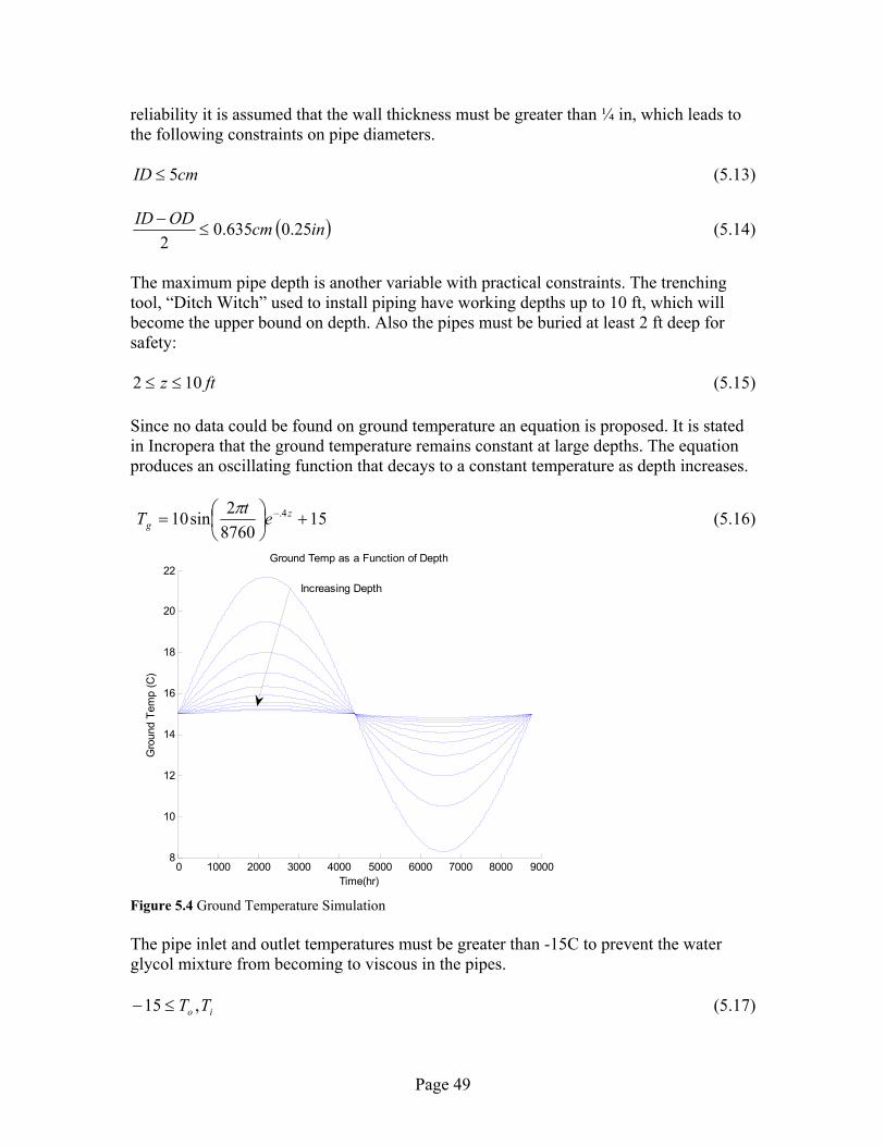
ftz 102 ≤≤ (5.15) Since no data could be found on ground temperature an equation is proposed. It is stated in Incropera that the ground temperature remains constant at large depths. The equation produces an oscillating function that decays to a constant temperature as depth increases.

1587602sin10 4. +⎟

⎠⎞

⎜⎝⎛= − z

g etT π (5.16)

0 1000 2000 3000 4000 5000 6000 7000 8000 90008

10

12

14

16

18

20

22

Time(hr)

Gro

und

Tem

p (C

)

Ground Temp as a Function of Depth

Increasing Depth

Figure 5.4 Ground Temperature Simulation The pipe inlet and outlet temperatures must be greater than -15C to prevent the water glycol mixture from becoming to viscous in the pipes.

io TT ,15 ≤− (5.17)

The final practical constraints are the greater than zero variables, which only exit in the positive real domain.

mDdLz ,,,,0 ≤ (5.18) 5.3.3 Variables and Parameters There are only three variables to be optimized for the GCHP system, the depth, length, and inner diameter of the buried pipe. Table 5.1 Variables for GCHP subsystem Variable Definition z Depth of buried pipe L Length of pipe ID Inner diameter of pipe During simulation there will be some functional values determined for each hour based on the input variables. They are listed and defined in the following table 5.2. Table 5.2 Variables determined in Simulation Function Definition m Mass flow rate hL Head Loss

iT Inlet temperature

oT Outlet temperature f Power The parameters used during simulation are listed below with their typical values. The ground temperature and heat rate, which are time dependant parameters, are given and sample value Table 5.3 Parameters for GCHP subsystem Parameter Definition Typical Value η Efficiency of the heat pump/exchanger 70% λ Surface roughness of the pipe 4.6E-6 m υ Kinematic viscosity of water 1.005E-6 m2/s ρ Water Density 998 kg/m3

pc Specific heat of water 4.2 kJ/kg K

pk Thermal conductivity for PVC pipe 0.47 W/m K

gT Ground temperature as a function of depth and time 15 C at 8ft

reqQ Heat rate for standard house as a function of time 5000 W

The degree of freedom for a system is the number of variable minus the equality constraints. For this system there are 3 variables with no equality constraints leaving 3 degrees of freedom.

A guess and check method was used to check for feasible solutions. For a single hour of operation the following feasible values were found after 3 iterations of guess and check. Table 5.4 Feasible solution set for GCHP subsystem Variable Feasible value z 5 m L 80 m ID .03 m Result Feasible value m .05 kg/s hL 0.714 m

oT 85 C

iT 17.5 C

gT 17 C

reqQ 4000 W

f (Power) 97 W 5.4 Summary Model

minimize f, ρ⋅⋅⋅= ∑=

gfi

8760

1

hL(i)(i)m

S.T. G1: 00.1-m ≤ G2: 05 ≤−hL G3: 0150 ≤−L G4: 02 ≤− z G5: 010 ≤−z G5: 005.0 ≤−ID G6-7: 0),(15 ≤−− io TT G8-12: 0,,,, ≤− mIDdLz 5.4 Simulation Model Explanation and Analysis 5.4.1 Simulation Method

There are two important quantities that must be simulation in order to run the optimization, the mass flow rate ( m ) and heat loss (hL). The functions which generate these values were coded in Matlab and then C++ to run in OPTIMUS. Head loss is dependant on mass flow rate, which was coded first. The mass flow rate function is dependant on the ground temperature, length of pipe, and the required heat rate. The flow rate must be determined from two equations, (5.8) and (5.4), therefore there will be two equations and three unknowns, flow rate, inlet temperature, and outlet temperature. This cannot be solved directly and in order to get a value for the flow rate a fixed point iteration method was used with the given values for the design variables and parameters. The system was initialized with all the water at ground temperature and a very small flow rate (0.001 kg/s). The ground temperature water was then run through the heat exchanger equation (5.4) to get an outlet temperature. The outlet temperature was checked for two conditions, boiling point (>90C) and freezing point (<-15C assuming that glycol was added to the water). If the outlet temperature was outside of the acceptable ranges the flow rate was increased incrementally until a feasible solution was found. The function stops when the inlet and outlet temperatures reach steady state as shown in figure 5.5.

0 2 4 6 8 10 12 14 1610

20

30

40

50

60

70

80

90

100

Iterations

Tem

p (C

)

Heat Pump Simulation To Steady State

Outlet Temp

Inlet Temp

Figure 5.5 Example steady state simulation of mass flow rate function

This function generates the smallest feasible mass flow rate given the chosen inputs. In order to avoid any type of control algorithm the transient performance of the pump was neglected, only steady state values of the flow rate and water temperatures were used. Essentially, it is assumed that the water in the system can change temperature instantaneously for every change in input value, which is reasonable for long periods of time and makes the problem much simpler. The flow rate can then be used along with the length and pipe diameter to calculate the heat loss. The code for head loss was adopt from an excel file found online

(Sellens) from a university website. It uses the inputs to calculate the flow characteristics such as Reynolds number and outputs the head loss after some internal iterations.

Both the flow rate and head loss functions are called by the main body code. The body reads the input values, generates the ground temperature and heat rate as functions of time, and outputs the required power. The heat rate is generated by the needs of the house, however without this information from the other subsystems a simple stepwise function was generated. During the spring/fall seasons the heat rate is relatively small and it peaks in the middle of winter and summer, see figure 5.6 for an example. It should be noted that a positive heat load corresponds to a need of cooling in the house; heat is being dumped into the system. One of the drawbacks of the simulation is that the heat load and ground temperature are represented as averages, the daily cyclic behavior is not modeled. This will be modified in further study and during collaboration with the other subsections.

0 1000 2000 3000 4000 5000 6000 7000 8000 9000

-5

0

5

10

15

20

25

Time(hr)

Ground Temp and Heat Load

Ground Temp C

Heat Load kW

Figure 5.6 Example of heat load and ground temperature over a year Originally the simulation was coded in MATLAB. However, the runtime of the code, about 40s, was too costly and could only run MATLAB optimizations. The code was revised and translated to a C++ executable, which runs in 0.5 sec on average. 5.4.2 Model Analysis

Conventional monotonicity analysis cannot be applied to this subsystem because the objective is the product of two simulated values; there are no formulae to examine. It may be possible to perform a DOE to determine monotonicity, however it was not attempted. The problem is however well bounded, each of the three optimization variables are bounded above and below by a simple constraint. In fact, for each variable there exits only a single upper and a single lower bound, which eliminates the possibility for redundancy.

Scaling was performed on the variables and output of the model. The goal of

scaling was to get nominal values within a single order of magnitude. To make thing simple the depth of pipe, 2-10 ft, was used as the standard order of magnitude. Table 5.5 shows typical values for un-scaled values, their scaling factor, and final results.

Table 5.5 Scaling for GCHP subsystem Variable Typical Values Scaling Factor Typical Scaled Values

L 15-150 0.1 5 ID 0.001-0.03 1000 3 z 2-10 1 6

Objective Typical Values Scaling Factor Typical Scaled Values f 1500 0.01 15

5.5 Numerical Results Optimization was attempted in both MATLAB and OPTIMUS. The long computational time of the MATLAB m code would not allow fmincon to run properly and optimization in MATLAB was abandoned. Once the code was transferred into C++ OPTIMUS ran without much difficulty and produced some good initial results. Three algorithms were used in OPTIMUS, differential evolution, simulated annealing and sequential quadratic programming (SQP). The first two algorithms require many function calls, 400+, and ran in approximately 5-7 minutes each. SQP used far fewer function calls and ran in approximately 2 min; however, the results were not as good as differential evolution or simulated annealing. There was a software issue with the generalized reduced gradient method (GRG) causing OPTIMUS to fail before the process could begin. GRG would have been the primary algorithm used, since it was studied heavily for this report. The issue will be resolved for future optimizations. The initial optimization was performed on a simulation with a 4000W peak heat load in the summer and a -4000W peak heat load in the winter. The results for each algorithm are shown in figure 5.7. The constraints used are: g1 =L-150; %Maximum length g2 =15-L; %Minimum length g3 =ID-.05; %Maximum ID g4 =.005-ID; %Minimum ID g5 =2-z; %Minimum depth g6 =z-10; %Maximum depth g7 =mdot - .3; %Maximum flow rate g8 =-mdot; %Minimum flow rate

0 5000 10000-5000

0

5000

Time (hrs)

Hea

t Loa

d (W

)

Figure 5.7 Initial GCHP Optimization in OPTIMUS The best optimization was produced by differential evolution with a f = 13.34. Upon examination of the variable values at the optimum it appear that the upper constraints on ID and pipe depth are both active at 5cm and 10 ft respectively. The activity of the ID bound makes sense physically. The ID has no influence on the required flow rate, and increased diameter allows a lower head loss, which decreases the required power. The depth of pipe is not as intuitive because the depth affects the decaying oscillation of the ground temperature. The other two algorithms made the ID active, but not the depth, which resulted in worse optimums. Further examination of the optimization process showed that both algorithms were in the process of increasing the depth when they finished, while the ID had achieved steady values. The length of the SQP algorithm is also inconsistent with the other two. These inconsistencies lead us to believe that the SQP and simulated annealing algorithms did not run enough iterations or got stuck in local minima. To check the local minima problem the algorithms were re-run with new starting points. Simulated annealing reached roughly the same optimum and optimal variables, while SQP reached roughly the same optimum, at different optimal point. Therefore the simulated annealing needs to run more iterations and the step size on the SQP may need to be adjusted to avoid local minima.

A simple parametric study was done with the simulation. The first variation was

o

nother parametric study was done to compare a home where the residents like it hot to a

to change the peak heat loads from 400W to 6000W as shown in figure 5.8. All three optimization algorithms were then run, however SQP had a fatal error and produced nuseable results. The results from differential evolution and simulated annealing made intuitive sense, a higher heat load requires longer pipes to dissipate the heat into the ground and more power to push water though a longer pipe. The power required increased from approximately 14 to 54 while the length increased from 5.5 to 10.

Figure 5.8 Parametric study results for increased heat load

0 5000 10000

-6000

-4000

-2000

0

2000

4000

6000

Time (hr)

Hea

t Loa

d (W

)

Ahome with colder inside temperatures. This produces non-symmetric heat load schedules. The magnitude of the heat loads for each of these cases is shown in figure 5.9 along with the results for the differential evolution.

0 5000 10000

-5000

0

5000

Time (hrs)

Hea

t Loa

d (W

)

0 5000 10000

-5000

0

5000

Time (hr)

Hea

t Loa

d (W

)Colder Room Hotter Room

Figure 5.9 Parametric Study for non-symmetric heat loads As the results show it takes much more power to keep a house hot (f = 88.6) than to keep

.6 Cost Assignment for System Optimization

order to optimize the entire system, including the four subsystems already described it

nd of

and

fixed cost. The fixed cost function is shown below:

a house cool (f = 16.1). The optimum is therefore sensitive to large heating demands in the winter. Practically this shows that GCHP systems are much more suited for warmer climates were only cooling is required. The difficulty in heating a house is pulling the needed heat load from a cold ground in the winter, whereas, it is much easier to dump heat into the ground in the summer. 5 Inwas decided to minimize cost over a 20 operational period. For the GHCP subsystem the costs will include the initial fixed costs of construction and a present value of the operating costs. The fixed cost of the water pipes was found using the cost per poucopper, $1.35 ( http://www.corriente.com/coppernews.htm ) and adding 50% for formingcost. The cost instillation was based on the assumption that it takes 1 hour per meter length per foot depth to dig the ditch, lay the pipe, and fill the hole. The cost of labor equipment rental was assumed to be $15/hr. The pump cost ($2000) is also added to the

2000$15$5.135.1$44

22

⎟⎞

⎜⎛ IDOD

+⋅⋅+⋅⋅⋅⎟⎠

⎜⎝

−⋅= zLLCost copperρπ (5.19)

The operation costs were based solely on the electricity needed to run the pump evaluated t present value. Maintenance was not incorporated into the operating costs for

r:

Fixed

asimplicity. The going rate at DTE for electricity is $0.07 per kWHr which was incorporated into the cost function, using the present value formulae from earlie

⎟⎠⎞

⎜⎛ ⋅= 07.0$ PowerPVCost ⎝ 1000

.0 All-in-One System

compiled in Optimus. The Wall, Window & Door, and olar Panel subsystems were compiled as a single model in MATLAB, while the Heat

mp.

Fixed

6 The entire system model wasSPump system ran through an .exe file coded in C++. The common objective of the problem was to minimize cost of operation of the house over 20 years. Initial costs were the material costs of the various subsystems, with continuous costs to run the heat puThe solar panel array was treated as a profit to the system, and was subtracted from the total cost. Therefore, the common objective function, total cost (Tcost) is given as:

))(cos(coscos HeatPumpsavingstSolarpanelDoorWindowWalltPVT t +−+++= (6.1)

The Solar panels, Windows & Doors, and Walls subsystems share common room imension variables that were once treated as subsystem parameters. The all-in-one

isting 6.1).

devaluation allowed for the systems to pass important values between each other. The entire system consists of 23 variables, 52 inequality constraints, and 1 equality constraint, excluding explicit upper and lower variable bounds. Below is a table lall of the variables, a feasible starting point, and upper and lower bounds (see Table Constraints: G1: 0)(2)( ≤+−+ WbLbWLWL drdrwinwin +vbn

0max ≤− floorLW G2: G3: 0min ≤− Ll G4: 0min ≤−Wwd G5: 0max ≤− bb

0≥x G6:

G7: 0≥z G8: 0≥vn

5.3≥b G9: G10: 0 5.0≥inst

12:

Lr ≤ 0

Wwall <0

<=0

r

or <=0

-

m <=0

G11/G k 001.008.0 ≥≥ ins

01.03 ≥≥ wt G13/G14:

G15: Lp - G16: Wp – Wr ≤ 0 G17: θ − π/2 ≤ 0 G19: φ - 2π ≤ 0 G20: Wdr - G21: Wwin - Wwall <0 G22: Wmindr - Wdr<=0 G23: bdr- (0.75 broom) G24: bwin - 0.75bdr <0 G25: bmind - bdr<=0 G26: Af - 0.25Aflo G27: I*Af 2.5 <0 G28: 0.8- Ldr <=0 G29: Ldr - 2<=0 G30: Lwin - 0.1* Lroo

G31: - Ao <=0 G32: ((0.8* Lwin* Wwin)- Af<=0

<=0

0

=0

t

6.1 Input array to imus Starting Value

Lower Bound

Upper Bound

0.3 0.01 20.3 .01 2

2

all) 3 32

00 0

0 0 0

1x13 bdr 2.3 0.01 10

G33: 8*Wwin - Lwin <=0 G34: 8*Wdr - Ldr G35: - Aglass <=0 G36: (0.008-w)<=0 G37:w-0.03 <=0 G38: L-150 <=0 G39: 15-L <=0 G40: ID-.05 <= G41: .005-ID <=0 G42: 2-z <=0 G43: z-10 <=0 G44: mdot - .3 < G45: -mdot <=0 H1: instzx =++ w

Table Opt

Designation Variable x1 x x2 tins 0x3 vn 2 1 0x4 z (wall) 0.1 0.01 2x5 b (w .6 .5 10x6 w (wall) 6 5 0x7 L (wall) 6 5 20x8 kins 1 .1 90x9 twall .7 .3 6x10 lwin .5 .01 3x11 bwin 1 .01 3x12 ldr 1 0.01 0

x14 w 8 0.01 1 11panel 1

f panel 0 6

r Diam

ss 0

10 Optimus’ SQP algorithm with a central difference method was used to calculate the m mizer of our cost function. The optimizer values, the optimum nction value, and

x - 0.01

0

00

Window Doors

00.902

dr

Solar Collector Optimize

θ of panel 0.φ of panel 0.657

Hea mp

2x15 wdr .5 0.01 15x16 θ of 0.5 0.01 .57x17 φ o .5 0.01 .28x18 Lp 4 0.01 50x19 L

Wp (pipe)

45

0.012

5015

ID Inne 3 1 4

TKPipethickne 1 .5 3

z Depth of pipe 5 2

ini fuactive constraints are shown below (see Table 6.2). Variables with a – next to them indicate that they are actively bounded below, variables with a + next to them indicate that they are actively bounded above. Table 6.2 Summary of results for All-in-one optimization Wall Design Variables Optimizer

tins 0.05vn 16.408z .239

b - 3.5w - 5L - 5k ins

t .08

wall - .3

s and lwin .42bwin l 0.806bdr w

2.28

wdr 10.7

r 4511

Lp - 0.01Wp -

0.01

t PuL - 2

ID + 45

st = optimum = $333 Table 6.3 Summary of active constraints

6.1 First Run Results and Discussion

ptimus. The minimum cost for the system

the variables involved in the wall design, for the full system semble the values obtained for the wall sub-system when

ptimized separately. For example, the wall height, b, and the room width and length, l most

e sulation

oth changed to their lower bounds of 0.05 and 0.01 meters. The amount of surface area re

he

Active Constraints

TK - z - 2Tco 0

G3 G4 G6 G9

G10 G12 G6

G16 G18 G25 G36 G7 G8

This section will discuss the results found by Owas found to be $3330 over 20 years. 6.1.1 Wall Design The optimal values foroptimization closely reoand w all fell on the lower bound as before, because the smallest room would be the economical to build and heat. Also, as before the optimal thermal conductivity for the wall insulation was found to be 0.08 W/mK, which represents the best thermal performance at the most economical cost according the cost function used. The wall thickness, however, changed 30% from 0.7 to 0.3, and consequently ththickness of the water container, z changed. The amount of inner and outer inbcovered by wall panels including water also went down from 19.14 to 16.408 squameters. Potential reasons for these differences can include the effects of the additional heat load from the doors and windows. When the wall sub-system was run independently, the door and window areas were treated as constant parameters. With t

entire system optimized as a whole, the door and window values were then vwhich dictate the dimensions of the room walls through several different constraints. Another factor that could have lead to differences in these optimal values is the differe

ariables

nce computed. For the wall sub-system the heat load was found by

e heat

.1.2 Roof-mounted Solar Panel Array

l array can be seen in x16 to x19 above. he values for Lp and Wp, the length and width of the roof covered in panels, both

e or

s is

s ormally would not make sense – θ and φ were around 60o and 234o in the single

, e to

or

mpiled and run together there was a bit difference in the ngth of the window, the height of the window, the length of the door and the height of

ence

in how cost wasintegrating the difference between the room temperature response and the desired room temperature of 23 degrees C. However, when the entire system was optimized thload was calculated separately from the heat pump model, and the cost for heating was different, thus driving variables involving wall dimension (and consequently insulation volume and initial costs) to a different optimum. 6 The minimizer values related to the solar paneTreached the lower bound assigned at 0.01m. 0.01m was chosen to prevent SQP from choosing values below 0 – occasionally Optimus would choose variable values abovbelow the allowed range, forcing us to artificially shrink the range of the variables. Therefore it can be seen that the optimum area of solar panels to use is 0 m2. This makes the solar panel cost function essentially equal to zero. A possible explanation for thithat at a total interest rate of 8%, the payback period for the panels is greater than m = 20yrs. This suggests that a smaller interest rate and a longer period would be desirable. Before the end of this project, a parametric study will be performed on these two parameters, but at their current values, it is not desirable to employ solar panels. The panel angles θ and φ are 25o elevation, facing 37o east of North. These valuensubsystem – but there is a possible explanation for this. With panel area nearly zerocollected energy becomes nearly zero, so the model becomes completely insensitivpanel angles. Therefore the algorithm would have no way of converging on a proper φθ, because the objective value is zero for all values of φ and θ. θ also could have been reduced because wall thickness from the Wall Design system was small. The roof therefore can not support as heavy a load as it could with thicker walls. 6.1.3 Windows & Doors When the whole system was colethe door. All these variables are interlinked with the wall design and the parameters which were used in the constraints like the wall height, wall length are now the variables and so that might have influenced some change in the variables. But there is no differin the height of the door and thickness of the individual glass. The length of the window decreased from 0.569 to 0.42, the height of the window increased from 0.5877 to 0.902, the length of the door increased very insignificantly from 0.8 to 0.81, the thickness of the

door increased very insignificantly from 0.10 to 0.11. The main influence for the change of these values are due to the length of the wall, the height of the wall, the thickness of the wall and the width of the room, which were the parameters in the previous subsystem has become variables in the all in one subsystem and thus they dominate certain constraint equations and thus a change is noticed from the values of the individual subsystem. 6.1.4 Ground Coupled Heat Pump (GCHP)

es are at a bound which minimizes ost, except for the ID variable which it at the most expensive bound. The reasons behind

e

ystem

ap

e to the effects of a higher interest rate when iscounting any future income to present value it was not economically practical to have

ure was

osts

n the interest rate was reduced 5%:

Summary of results for All-in-one optimization with the interest rate adjusted to 5% Variables Optimizer

0

w -

At the system optimal level all of the GHCP variablcthis outcome are rather clear. When the subsystem was optimized parameter values werused for the house heat load, while during the system optimization the required heat load was provided by the wall and doors subsystems. The parameter values during the subsystem were on the order of 5000 Watts per hour (found using a web based HVAC tool on www.carrier.com), while the values provided by the wall and window subswere an order of magnitude less. Operating with heat loads of 500 Watts per hour the GHCP model can meet the HVAC demands with minimal effort, which translates into a short pipe length (an expensive variable), provided a large enough pipe diameter (a chevariable). The bounds for the GCHP subsystem, and magnitude of the heat loads will be re-examined before another system optimization is preformed.

6.1.5 Effects of Interest Rate As seen in our optimal solution, dudsolar panels mounted on the roof. However, when the same optimization procedrun at a lower interest rate (5% instead of 8%) building the house with solar panels became practical as they began to generate income. In fact, the minimized objective value showed that after 20 years the solar panels would not only pay for the initial cof the house, but they would also begin to generate profit. Table 6.4 lists the variables and their optimal solutions wheto Table 6.4Wall Design

x - 0.01tins 0.05vn 20z .239

b - 3.59.79

L - 20kins 0.08twall - 0.3

Window an Doors

lwin 0.5990.654

8 Solar Collector Optim

θ of panel 0

Hea p

3.210

In Table 6.2, most of the variables remained close to the values obtained from the

ptimization with an interest rate of 8% with the exception of the room width and length.

d optimal solutions to each of our sub-tinue this project with

er The

e

e

s d

bwin ldr 0.80bdr 2.2w 8.1

wdr .31

izer .032

φ of panel 2.81Lp - 20Wp - 9.79

t PumL - 2

ID + TK - .5z - 2

oWith no solar panels, the most economical solution was to create a room with the minimum internal volume, thus the room width and length rested on their lower bounds. However, with an interest rate of 5%, building the solar panels became feasible, and now the income generated by the solar panels changed the roof (and consequently floor) area. The floor length now rests on the upper bound and the width has been changed to 9.79. In this case, the drawbacks of a larger floor area and interior volume has been offset by the income generated by the solar panels (which demand a larger surface area). 7.0 Conclusions and Further Work From our efforts, we were able to not only fin

stems but also for the all-in-one system. If we were to consyintents of building an actual home, we would refine our models for accuracy. For example, the wall heat transfer model should be updated to use a PDE to ensure propaccuracy. The solar array model could be improved by accounting for cloudy days.model for the windows should account for radiation emissivity and the optimal glass typshould also be considered. The heat pump system model would incorporate a model of an actual heat exchanger and would also be updated with accurate ground temperature data. With these further improvements, an optimization would be run and compared with our current results. Additionally, we would need to model a standard house and comparthe model results to our optimal solution. Thus, a true measure of cost savings can be established and this would aid in justifying the construction and sale of our optimal design.

8.0 References "Sun-Ray Solar http://members.cox.net/sunraysolar/index.html." Bouchlaghem and Letherman (1990). "Numerical Optimization Applied to the Thermal Design of Buildings." Building and Environment 25(2). DeWitt, I. a. (1996). Fundamentals of Heat and Mass Transfer. New York, John Wiley and Sons. Detroit Edison Energy, "Residential Electric Rates", http://my.dteenergy.com/myAccount/rates.do U.S. Naval Observatory, Astronomical Applications Dept. " Sun or Moon Altitude/Azimuth Table for One Day".http://aa.usno.navy.mil/data/docs/AltAz.html Scwolsky, R. and J. Williams (1982). The Builder's Guide to Solar Construction. New York, McGraw-Hill, Inc. Shigley, J. (2001). Mechanical Engineering Design. New York, McGraw-Hill. Young, W.C. (2002). Roark's Formulas for Stress and Strain (7th Ed.) 502-503,527. New York, McGraw-Hill, Inc. Zaheer-Uddin, M. (1986). "A Two-component Thermal Model for a Direct Gain Passive House With a Heated Basement." Building and Environment 21(1): 22-33. ASHRAE Fundamental Handbook 1997 http://www.memsnet.org/material/silicondioxidesio2bulk/

Development of a revised Cooling and Heating Load Calculation Manual Spitler, J.D. (Oklahoma State Univ); McQuiston, F.C.; Lindsey, K.L. Source ASHRAE Transactions, v 99, n pt 1, 1993, p 175-182 Heat Loss Calculations :-http://www.fe.psu.edu/~dxm15/aet121/Ch10HeatLoss.htm

Refrigeration and Air Conditioning Engineering by Arora and Domkundwar

NFRC website - http://www.nfrc.org/factsheets.aspx Building and Zoning Specifications:-http://www.cityofalliance.net/id26.htm Doors and Windows specification: http://www.vpaf.uni.edu/facplan/Content/pdf/DIVISION%208%20-%20DOORS%20AND%20WINDOWS.pdf

Monthly Climatic Information:-

onthly+Climateroduct=CLMDTW.0502012006&format=print

art.shtml

pumps.com/waterpumps.htm.

Retrieved 2/5/2005, 2005, 59.html.

D-

http://www.crh.noaa.gov/dtx/wxnow/product.php?site=dtw&title=M+Summary&p Psychometric Properties:- http://www.connel.com/freeware/psych "Amos Water Pumps - PM81." Retrieved 2/6/2005, 2005, from http://www.amos (2005). "Calculating Flow Rates in Heating Systems." from http://www.engineeringtoolbox.com/38_6 Ball, D. A., R. D. Fischer, et al. (1983). DESIGN METHODS FOR GROUNSOURCE HEAT PUMPS, Washington, DC, USA, ASHRAE, Atlanta, Ga, USA. Bose, J. E. and J. D. Parker (1983). GROUND-COUPLED HEAT PUMP RESEARCH, Washington, DC, USA, ASHRAE, Atlanta, Ga, USA.

Cane, R. L. D. and D. A. Forgas (1991). Modeling of ground-source heat pumpperformance, New York, NY, USA, Publ by ASHRAE, Atlanta, GA, USA.

t al. (1996). Thermal performance of horizontal Jones, W. V., Jr., J. T. Beard, eclosed-loop ground-coupled heat pump systems using flowable-fill, Washington, DC,

P. (1985). Simulation and experimental verification of vertical groun klahoma State. Ph.D.

USA, IEEE, Piscataway, NJ, USA. Kavanaugh, S.dcoupled heat pump systems. Stillwater, O Langley, B. C. (1989). Heat Pump Technology. Englewood Cliffs, Prentice-Hall.

om

niversity, O. S. (2005). "Building and Environmental Thermal Systems Group."

Sellens, R. (1998). "Friction Losses in Pipes." Retrieved 2/5/2005, 2005, frhttp://me.queensu.ca/courses/MECH241/piping_losses.htm. URetrieved 2/5/2005, 2005, from http://www.hvac.okstate.edu/.

thermally efficient house final report - welcome to...

Documents