thermal remediation behavior in high and low permeability
TRANSCRIPT
Thermal Remediation Behavior in High and Low Permeability
SystemsRon FaltaProfessor
Clemson University
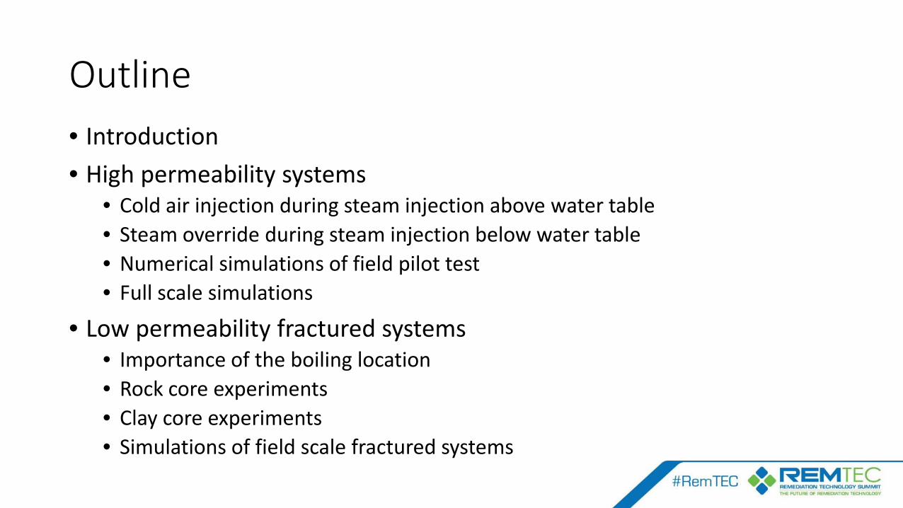
Outline• Introduction • High permeability systems
• Cold air injection during steam injection above water table• Steam override during steam injection below water table• Numerical simulations of field pilot test• Full scale simulations
• Low permeability fractured systems• Importance of the boiling location• Rock core experiments• Clay core experiments• Simulations of field scale fractured systems
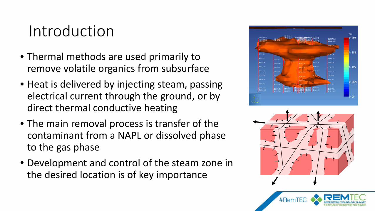
Introduction• Thermal methods are used primarily to
remove volatile organics from subsurface• Heat is delivered by injecting steam, passing
electrical current through the ground, or by direct thermal conductive heating
• The main removal process is transfer of the contaminant from a NAPL or dissolved phase to the gas phase
• Development and control of the steam zone in the desired location is of key importance

High Permeability: Steam Injection Below the water table
• Steam is much less dense than water• There is a tendency for steam to rise due to buoyancy
forces• This can cause steam override, resulting in poor contact
with contaminated zone• Tendency is proportional to ratio of permeability to steam
mass flux (van Lookeren, 1983; Basel and Udell, 1989)
• Strong permeability anisotropy reduces this effect

Numerical Simulations of Steam Injection into the Regional Gravel Aquifer, Paducah, KY
• Use the DOE TMVOC multiphase flow numerical code with the PetraSim interface
• Simplified r-z radially symmetric model around a single steam injection well
• RGA formation has very high K; bounded by lower K UCRS and McNairy formations
• Water table is located just above the top of the RGA
• Simulate steam injection into two screens at 500 lbs/hr each
• Perform simulations over a range of horizontal K and anisotropy values
Ground surface, opento atmosphere, 15 C
No flow boundary at bottom of grid
120 ftSteamInjection
UCRS, 0 to 60 ft; kh= 1.e-13 m^2; kz=1.e-14 m^2
McNairy, 90 to 120 ft; kh= 1.e-13 m^2; kz=1.e-14 m^2
RGA, 60 to 90 ft
Numerical Grid used for Simulations

Simulation of Steam Injection at 500 lbs/hr into each screen; Kh=200 ft/d Kv=20 ft/d (10:1)
Temperature after 10 days Temperature after 30 days Gas saturation after 30 days
Top of steam zone extendsto a radius of 35 ft
Bottom of steam zone extendsto a radius of 7 ft

H2O Mass Flux Vectors and Gas Saturation at 30 Days

Steam Pilot Test at C-400, DOE Paducah Gaseous Diffusion Plant• 2015 test performed by ERM
and Fluor Federal Services (Dablow, et al., 2016)
• Phase I: inject steam at 500 lb/hr into two screens for 20 days
• Phase II: 14 day cool down• Phase III: Inject steam into lower
screen only at 1000 lb/hr• Monitor temperature at 186
points in 11 vertical arrays
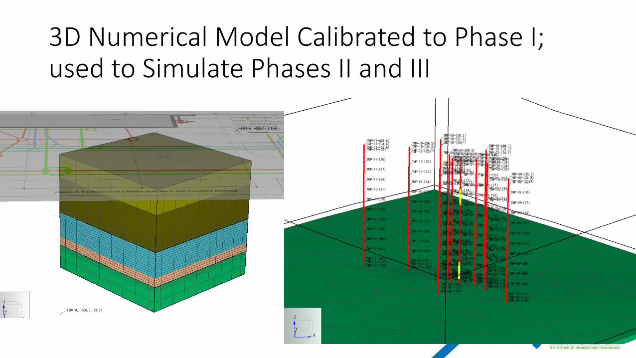
3D Numerical Model Calibrated to Phase I; used to Simulate Phases II and III
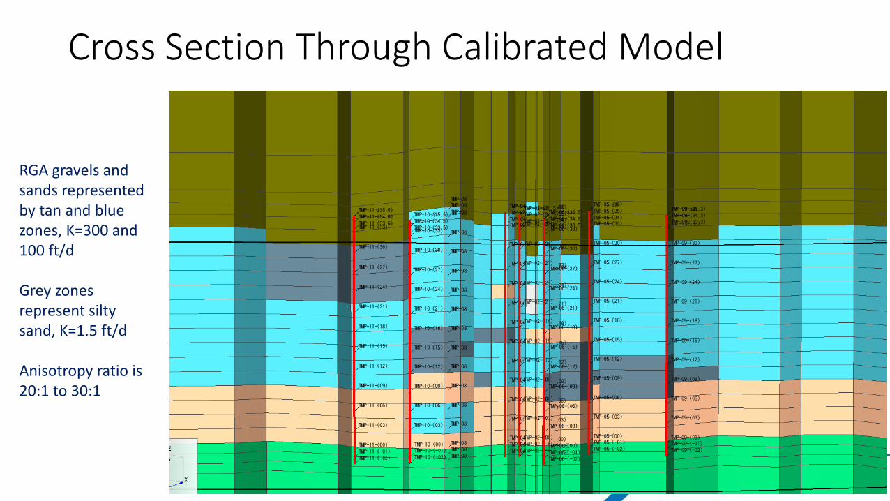
Cross Section Through Calibrated Model
RGA gravels and sands represented by tan and blue zones, K=300 and 100 ft/d
Grey zones represent silty sand, K=1.5 ft/d
Anisotropy ratio is 20:1 to 30:1

Simulated and Observed Temperatures at the end of Phase I Injection
-5
0
5
10
15
20
25
30
35
40
50 100 150 200 250 300
Heig
ht a
bove
bas
e of
RG
A, ft
Temperature, F
TMP-10, 04-29-2015 06:00:00
measured Temp
model
-5
0
5
10
15
20
25
30
35
40
50 100 150 200 250 300
Heig
ht a
bove
bas
e of
RG
A, ft
Temperature, F
TMP-11, 04-29-2015 06:00:00
measured Temp
model
-5
0
5
10
15
20
25
30
35
40
50 100 150 200 250 300
Heig
ht a
bove
bas
e of
RG
A, ft
Temperature, F
TMP-07, 04-29-2015 06:00:00
measured Temp
model
-5
0
5
10
15
20
25
30
35
40
45
50 100 150 200 250 300
Heig
ht a
bove
bas
e of
RG
A, ft
Temperature, F
TMP-08, 04-29-2015 06:00:00
measured Temp
model
-5
0
5
10
15
20
25
30
35
40
50 100 150 200 250 300
Heig
ht a
bove
bas
e of
RG
A, ft
Temperature, F
TMP-09, 04-29-2015 06:00:00
measured Temp
model
-5
0
5
10
15
20
25
30
35
40
50 100 150 200 250 300
Heig
ht a
bove
bas
e of
RG
A, ft
Temperature, F
TMP-01, 04-29-2015 06:00:00
measured Temp
model
-5
0
5
10
15
20
25
30
35
40
50 100 150 200 250 300
Heig
ht a
bove
bas
e of
RG
A, ft
Temperature, F
TMP-02 04-29-2015 06:00:00
measured Temp
model
-5
0
5
10
15
20
25
30
35
40
50 100 150 200 250 300
Heig
ht a
bove
bas
e of
RG
A, ft
Temperature, F
TMP-03, 04-29-2015 06:00:00
measured Temp
model
-5
0
5
10
15
20
25
30
35
40
50 100 150 200 250 300
Heig
ht a
bove
bas
e of
RG
A, ft
Temperature, F
TMP-05, 04-29-2015 06:00:00
measured Temp
model
-5
0
5
10
15
20
25
30
35
40
50 100 150 200 250 300
Heig
ht a
bove
bas
e of
RG
A, ft
Temperature, F
TMP-06, 04-29-2015 06:00:00
measured Temp
model
-5
0
5
10
15
20
25
30
35
40
50 100 150 200 250 300
Heig
ht a
bove
bas
e of
RG
A, ft
Temperature, F
TMP-04, 04-29-2015 06:00:00
measured Temp
model

Simulated Steam Zone at End of Phase I Injection

Simulated and Observed Temperatures near the end of Phase III Injection
-5
0
5
10
15
20
25
30
35
40
50 100 150 200 250 300
Heig
ht a
bove
bas
e of
RG
A, ft
Temperature, F
TMP-01, 05-27-2015 07:00:00
measured Temp
model
-5
0
5
10
15
20
25
30
35
40
50 100 150 200 250 300
Heig
ht a
bove
bas
e of
RG
A, ft
Temperature, F
TMP-02 05-27-2015 07:00:00
measured Temp
model
-5
0
5
10
15
20
25
30
35
40
50 100 150 200 250 300
Heig
ht a
bove
bas
e of
RG
A, ft
Temperature, F
TMP-03, 05-27-2015 07:00:00
measured Temp
model
-5
0
5
10
15
20
25
30
35
40
50 100 150 200 250 300
Heig
ht a
bove
bas
e of
RG
A, ft
Temperature, F
TMP-04, 05-27-2015 07:00:00
measured Temp
model
-5
0
5
10
15
20
25
30
35
40
50 100 150 200 250 300
Heig
ht a
bove
bas
e of
RG
A, ft
Temperature, F
TMP-05, 05-27-2015 07:00:00
measured Temp
model
-5
0
5
10
15
20
25
30
35
40
50 100 150 200 250 300
Heig
ht a
bove
bas
e of
RG
A, ft
Temperature, F
TMP-06, 05-27-2015 07:00:00
measured Temp
model
-5
0
5
10
15
20
25
30
35
40
50 100 150 200 250 300
Heig
ht a
bove
bas
e of
RG
A, ft
Temperature, F
TMP-07, 05-27-2015 07:00:00
measured Temp
model
-5
0
5
10
15
20
25
30
35
40
45
50 100 150 200 250 300
Heig
ht a
bove
bas
e of
RG
A, ft
Temperature, F
TMP-08, 05-27-2015 07:00:00
measured Temp
model
-5
0
5
10
15
20
25
30
35
40
50 100 150 200 250 300
Heig
ht a
bove
bas
e of
RG
A, ft
Temperature, F
TMP-09, 05-27-2015 07:00:00
measured Temp
model
-5
0
5
10
15
20
25
30
35
40
50 100 150 200 250 300
Heig
ht a
bove
bas
e of
RG
A, ft
Temperature, F
TMP-10, 05-27-2015 07:00:00
measured Temp
model
-5
0
5
10
15
20
25
30
35
40
50 100 150 200 250 300
Heig
ht a
bove
bas
e of
RG
A, ft
Temperature, F
TMP-11, 05-27-2015 07:00:00
measured Temp
model

Simulated Steam Zone at End of Phase III Injection
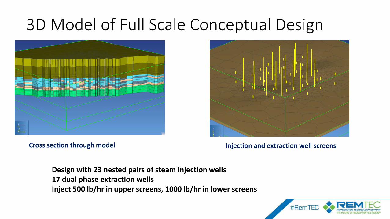
3D Model of Full Scale Conceptual Design
Cross section through model Injection and extraction well screens
Design with 23 nested pairs of steam injection wells17 dual phase extraction wellsInject 500 lb/hr in upper screens, 1000 lb/hr in lower screens

Simulated Temperatures after 10 and 20 days of Steam Injection
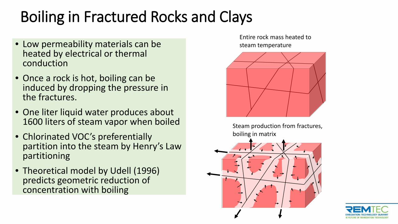
Boiling in Fractured Rocks and Clays• Low permeability materials can be
heated by electrical or thermal conduction
• Once a rock is hot, boiling can be induced by dropping the pressure in the fractures.
• One liter liquid water produces about 1600 liters of steam vapor when boiled
• Chlorinated VOC’s preferentially partition into the steam by Henry’s Law partitioning
• Theoretical model by Udell (1996) predicts geometric reduction of concentration with boiling
Entire rock mass heated to steam temperature
Steam production from fractures, boiling in matrix
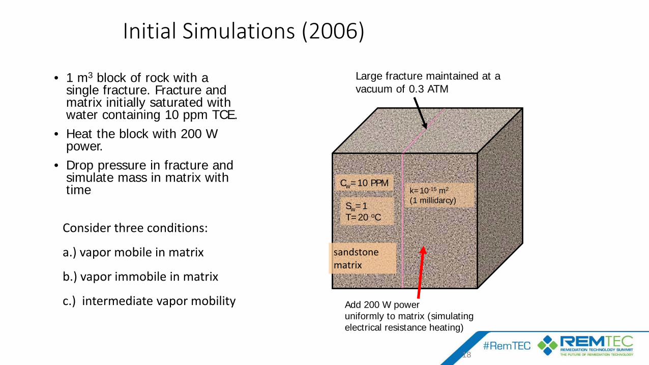
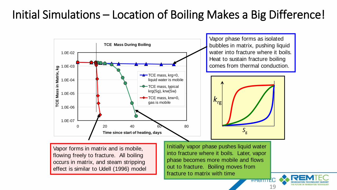
Initial Simulations (2006)
• 1 m3 block of rock with a single fracture. Fracture and matrix initially saturated with water containing 10 ppm TCE.
• Heat the block with 200 W power.
• Drop pressure in fracture and simulate mass in matrix with time Cw=10 PPM
Large fracture maintained at avacuum of 0.3 ATM
k=10-15 m2
(1 millidarcy)Sw=1T=20 oC
Add 200 W poweruniformly to matrix (simulatingelectrical resistance heating)
sandstonematrix
Consider three conditions:
a.) vapor mobile in matrix
b.) vapor immobile in matrix
c.) intermediate vapor mobility
18
TCE Mass During Boiling
1.0E-07
1.0E-06
1.0E-05
1.0E-04
1.0E-03
1.0E-02
0 20 40 60 80Time since start of heating, days
TCE
Mas
s in
Mat
rix, k
g
TCE mass, krg=0,liquid water is mobile
TCE mass, typicalkrg(Sg), krw(Sw)
TCE mass, krw=0,gas is mobile
Vapor phase forms as isolated bubbles in matrix, pushing liquid water into fracture where it boils. Heat to sustain fracture boiling comes from thermal conduction.
Vapor forms in matrix and is mobile, flowing freely to fracture. All boiling occurs in matrix, and steam stripping effect is similar to Udell (1996) model
Initially vapor phase pushes liquid water into fracture where it boils. Later, vapor phase becomes more mobile and flows out to fracture. Boiling moves from fracture to matrix with time
Sg
krg
Initial Simulations – Location of Boiling Makes a Big Difference!
19

Laboratory Experiments
Field Scale Fracture-matrix interactionis locally ~ 1-D
Unfractured matrix material (silt, clay, limestone, sandstone, etc.)
Simulated fracture on one end

Experimental Design – Rock Cores
1. Contaminate matrix by pumping contaminated water through it at a high pressure gradient until concentrations stabilize at the outlet. This is only possible at higher permeabilities (~100 millidarcy)
Inject water with 1,2-DCA, NaBr.Produce water
2. Seal and insulate column, turn on heaters, open fracture to atmosphere. Measure T, Sw, steam flow rate, contaminant flow rate at outlet.
heat
no flowopen
21Chen et al., 2010
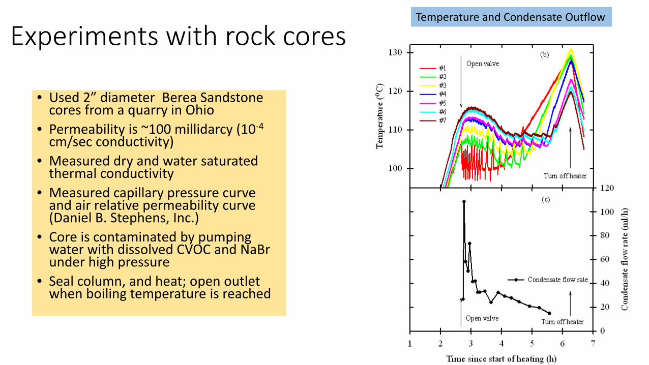
Experiments with rock cores
• Used 2” diameter Berea Sandstone cores from a quarry in Ohio
• Permeability is ~100 millidarcy (10-4
cm/sec conductivity)• Measured dry and water saturated
thermal conductivity• Measured capillary pressure curve
and air relative permeability curve (Daniel B. Stephens, Inc.)
• Core is contaminated by pumping water with dissolved CVOC and NaBrunder high pressure
• Seal column, and heat; open outlet when boiling temperature is reached
22
Temperature and Condensate Outflow

Experimental Results – cumulative CVOC removal
The core pore volume is 116 ml23

Experiments with clay cores (Liu et al., 2013)
• Pure kaolin clay mixed with water at optimum water content (maximum density)
• Permeability extremely low, ~ 100 microdarcy (~10-7 cm/sec)
• Water used to make clay was contaminated with 1,2-DCA
• Clay is packed into two 2” Teflon heat shrink tubes; one serves as a control to establish starting soil concentrations
• After heating to a certain point (for example 40% water removal), core is removed, and sliced for soil sampling
24
Water content (by weight): 0.43±0.02Selected for maximum density; pore volume is 260 ml and k=~10-16m2
25
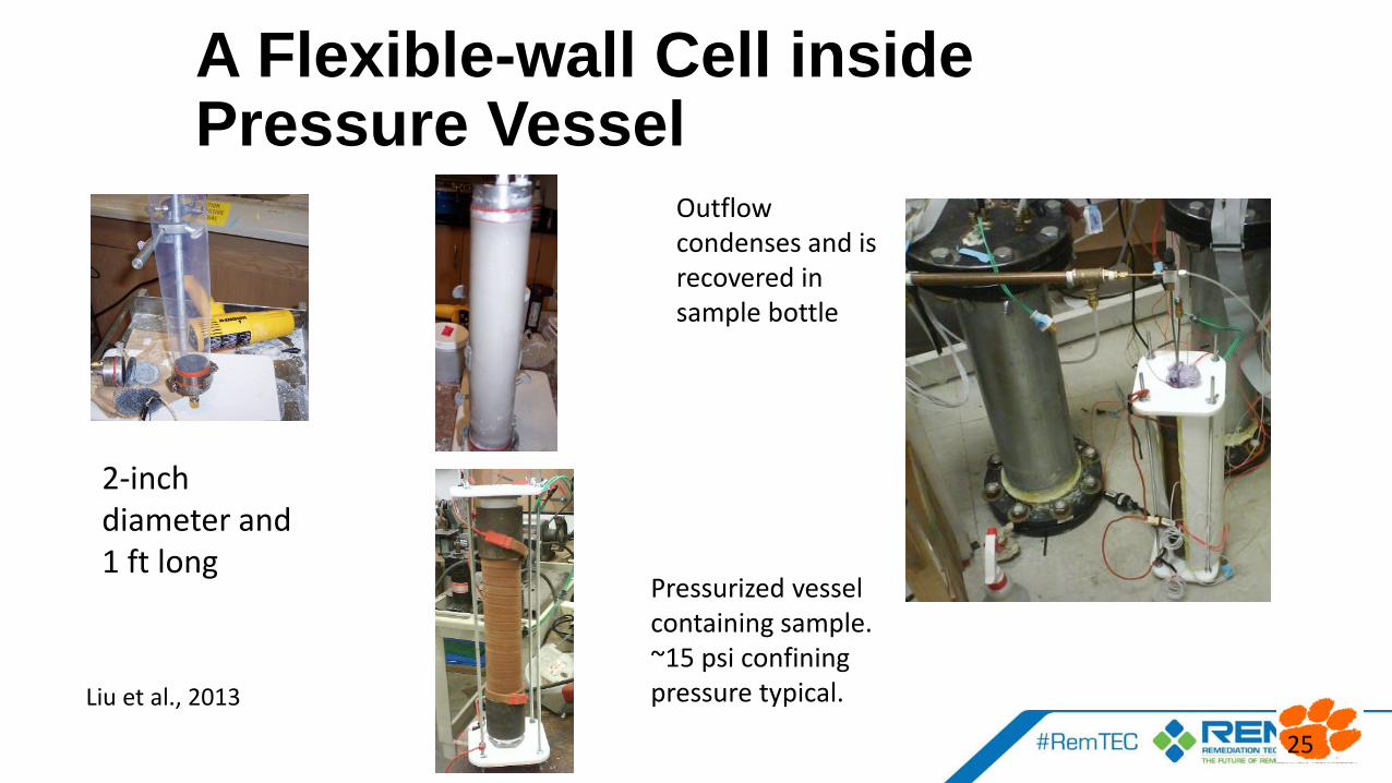
A Flexible-wall Cell inside Pressure Vessel
2-inch diameter and 1 ft long
Pressurized vessel containing sample. ~15 psi confining pressure typical.
Outflow condenses and is recovered in sample bottle
Liu et al., 2013

Sampling and Analysis – Destructive Sampling During Many Repeat Experiments
Water Content along core by oven drying samples
DCA concentraction remaining in the clay using a.) headspace extraction and b.) methanol extraction
Solids- slice up the coresbefore and after heating

Results of 8 different experiments that are stopped at different times and sliced apart
0.0001
0.001
0.01
0.1
1
10
0 5 10 15 20 25
DCA
rela
tive
conc
entr
atio
n
Sample length (cm, from bottom to top)
DCA profiles in clay cores with different fractions of pore water boiled out. IN is initial DCA concentration
IN, with error bar
6%
10%
19%
29%
39%
66%
67%
53%
27

28
Fractures!

Field scale simulations of fractured systems
• Numerically challenging due to small size of fractures compared to large size of model
• Large contrasts in permeability and capillary pressure between fractures and rock matrix
• Discretization issues – need to discretize both the fractures (very small) and the matrix (very large), with transitions in size between the two
29

Multiple Interacting Continua (MINC) discretization
Electrode ElectrodeVacuum Well
Insulating Cover
Water Table
Groundwatercontaminated with10 PPM of TCE inboth fracturesand matrix
16 m
Fractured Limestone
Electrode ElectrodeVacuum Well
Insulating Cover
Water Table
Groundwatercontaminated with10 PPM of TCE inboth fracturesand matrix
16 m
Fractured Limestone
Spatial domain is discretized normally into volume elements
Each gridblock is subdivided into a fracture element, and multiple nested matrix elements. The fracture and matrix elements are locally connected to each other in 1-D
fractures
matrix blocks
The fracture elements are globally connected in all directions.
This is similar to a dual porosity formulation, but gradients in the matrix are resolved much more accurately
30

Field Simulation Example (Chen et al., 2015)
Electrode ElectrodeVacuum Well
Insulating Cover
Water Table
Groundwatercontaminated with10 PPM of TCE inboth fracturesand matrix
16 m
Fractured Limestone
Electrode ElectrodeVacuum Well
Insulating Cover
Water Table
Groundwatercontaminated with10 PPM of TCE inboth fracturesand matrix
16 m
Fractured Limestone
Idealized field scalesimulation – single elementof a repeated 6-phase electrical heating pattern.
3-D orthogonal set of 200 micron fractures with 1m spacing, matrix k=10-15 m2; model uses MINC for matrix blocks.
Add 800 kW (200W/m3)power for 15 days, then pump vacuum well at 0.5 ATM for 1 year. Re-energize for 3 days and pump vacuum well for another year

Simulation Result
20
30
40
50
60
70
80
90
100
110
120
0 100 200 300 400 500 600 700
time, days
Ave
rage
Tem
pera
ture
, C
0
100
200
300
400
500
600
700
Stea
m E
xtra
ctio
n R
ate,
Lite
rs/m
in
Temperature
Steam ExtractionRate 0.1
1
10
100
1000
10000
0 100 200 300 400 500 600 700
time, days
Ave
rage
TC
E C
once
ntra
tion,
ug/
l
0
0.1
0.2
0.3
0.4
0.5
0.6
0.7
0.8
0.9
1
Ave
rage
Wat
er S
atur
atio
n
TCE
SwRe-e
nerg
ize
Re-e
nerg
ize
32
Simulations with lower matrix permeability show a slower reduction of TCE concentration with time
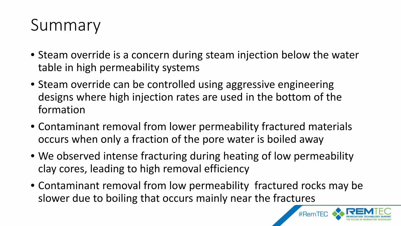
Summary• Steam override is a concern during steam injection below the water
table in high permeability systems• Steam override can be controlled using aggressive engineering
designs where high injection rates are used in the bottom of the formation
• Contaminant removal from lower permeability fractured materials occurs when only a fraction of the pore water is boiled away
• We observed intense fracturing during heating of low permeability clay cores, leading to high removal efficiency
• Contaminant removal from low permeability fractured rocks may be slower due to boiling that occurs mainly near the fractures