thermal modelling site descriptive modelling laxemar – stage 2 · domains: rsma (Ävrö granite),...
TRANSCRIPT

Thermal modelling
Site descriptive modelling
Laxemar – stage 2.1
John Wrafter, Jan Sundberg, Märta Ländell, Pär-Erik Back
Geo Innova AB
December 2006
R-06-84
R-0
6-8
4Th
ermal m
od
elling
. Site d
escriptive m
od
elling
. Laxemar – stag
e 2.1
Svensk Kärnbränslehantering ABSwedish Nuclear Fueland Waste Management CoBox 5864SE-102 40 Stockholm Sweden Tel 08-459 84 00 +46 8 459 84 00Fax 08-661 57 19 +46 8 661 57 19
CM
Gru
ppen
AB
, Bro
mm
a, 2
007

Thermal modelling
Site descriptive modelling
Laxemar – stage 2.1
John Wrafter, Jan Sundberg, Märta Ländell, Pär-Erik Back
Geo Innova AB
December 2006
ISSN 1402-3091
SKB Rapport R-06-84
This report concerns a study which was conducted for SKB. The conclusions and viewpoints presented in the report are those of the authors and do not necessarily coincide with those of the client.
A pdf version of this document can be downloaded from www.skb.se

�
Summary
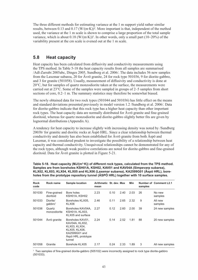
This report presents the thermal site descriptive model for the Laxemar subarea, version 2.1. The main objectives of this report are to present a current thermal model based on available data, to identify remaining issues of importance, and to give recommendations regarding future data requirements. The modelling work is based on quality controlled data available at the time of data freeze Laxemar 2.1. The data has been evaluated and summarised in order to make an upscaling to rock domain level possible.
The thermal conductivity at canister scale has been modelled for five different lithological domains: RSMA (Ävrö granite), RSMBA (mixture of Ävrö granite and fine-grained dioritoid), RSMD (quartz monzodiorite), RSME (diorite/gabbro) and RSMM (mix domain with high frequency of diorite to gabbro). A base modelling approach has been used to determine the mean value of the thermal conductivity. Spatial variability of thermal conductivity at domain level has been evaluated by making judgements based on the results of the alternative/com-plementary approaches used in Laxemar model version 1.2. Thermal modelling is based on the rock domain model for the Laxemar subarea, version 1.2 together with thermal rock type models based on measured and calculated (from mineral composition) thermal conductivities. For one rock type, Ävrö granite, density loggings have also been used in the domain modelling in order to evaluate the spatial variability within this rock type. This has been possible due to an established relationship between density and thermal conductivity, valid for the Ävrö granite.
Results indicate that the means of thermal conductivity for the various domains are expected to exhibit a variation from 2.56 W/(m·K) to 2.79 W/(m·K). The standard deviation varies according to the scale considered, and for the 0. 8 m scale it is expected to range from 0.28 to 0.�6 W/(m·K).
For Laxemar model stage 2.1, thermal conductivity has been estimated for the same five rock domains previously described in the Laxemar model version 1.2. For domain RSMA, the mean thermal conductivity is somewhat lower and the standard deviation significantly higher in the current model version compared to the previous version. For domain RSMD, both the mean and standard deviation are somewhat higher in Laxemar 2.1, an effect of the higher proportion of rock type fine-grained granite, which imparts a pronounced upper tail to the distribution. Although the mean thermal conductivity for domain RSMM shows little change from model version 1.2, variability, as expressed by the standard deviation, is significantly higher. Uncertainty remains high for this domain due to the lack of representative borehole data and a poorly constrained statistical model for diorite-gabbro.
Domain modelling of heat capacity has not been performed as part of this model version. The new data presented here is unlikely to influence the results of domain modelling presented in model version 1.2.
The mean measured coefficient of thermal expansion for the investigated rock types varies between 6.9·10–6 and 7.9·10–6 m/(m·K) (1.7·10–6 m/(m·K) is the highest standard deviation).
In situ temperature has been measured in six boreholes in the Laxemar subarea. It was concluded from an evaluation of the temperature loggings that data from only two boreholes, KLX02 and KLX05, is of sufficiently high quality. Uncertainties in the data from other bore-holes relate to problems associated with calibration of the logging probe, in addition to logging too soon after drilling, i.e. before temperature conditions stabilized. The mean temperature at 500 m depth for these two boreholes is 14.6°C, which compares with 1�.9°C reported in model version 1.2.
4
Uncertainties associated with the reported results include choice of the representative scale for the canisters, methodological uncertainties associated with the upscaling of thermal conductivity from centimetre scale to canister scale, representativeness of rock samples, the effect of alteration, potential bias in the calculated thermal conductivity values from density loggings, and possible bias in heat capacity data. The current model version has produced some reductions in uncertainties. More specifically, the statistical relationship between density and thermal conductivity for Ävrö granite has been improved, measurement data on rock types are considered to be more representative, statistical rock type models are in some cases more certain, and the rock volume is represented by more boreholes. In addition, errors associated with temperature logging have been defined, and poor quality logging data has been excluded from calculations of mean temperatures for various depths.

5
Sammanfattning
Föreliggande rapport presenterar den termiska platsbeskrivande modellen för Laxemarområdet, version 2.1. Syftet med denna rapport är att presentera den termiska modellen, baserad på befintliga data, identifiera kvarvarande frågeställningar och ge rekommendationer beträffande framtida data behov. Modelleringsarbetet är baserat på kvalitetskontrollerade data tillängliga vid datafrysen för Laxemar 2.1. Data har utvärderats och sammanfattats för att möjliggöra en uppskalning till litologisk domännivå.
Den termiska konduktiviteten i kapselskala har modellerats för fem olika litologiska berg-domäner (RSMA (Ävrö granit), RSMBA (blandning av Ävrögranit och finkornig dioritoid), RSMD (kvartsmonzodiorit), RSME (diorit/gabbro) och RSMM (blanddomän med stor förekomst av diorit och gabbro)). Ett grundläggande angreppssätt (base approach) för den ter-miska modelleringen har använts för bestämning av den termiska konduktivitetens medelvärde. Värmeledningsförmågans rumsliga variabilitet på domännivå har utvärderats även genom bedömningar baserade på resultaten av komplementerande angreppssätt som använts i Laxemar modellen, version 1.2. Den termiska modelleringen baseras på den litologiska domänmodellen för Laxemarområdet version 1.2 tillsammans med termiska bergartsmodeller upprättade med utgångspunkt ifrån mätningar och beräkningar (utifrån mineralsammansättning) av den termiska konduktiviteten. För en bergart, Ävrö granit, har densitetsloggningar inom den specifika bergarten också använts i domänmodelleringen för att uppskatta den spatiala variationen inom denna bergart. Detta har varit möjligt på grund av ett presenterat samband mellan densitet och termisk konduktivitet, gällande för Ävrö granit.
Resultaten indikerar att medelvärdet för den termiska konduktiviteten förväntas variera mellan 2,56 W/(m·K) till 2,79 W/(m·K) mellan de olika domänerna. Standardavvikelsen varierar beroende på vilken skala som bedöms. För kapselskalan (0,8 m) förväntas den variera mellan 0,28 och 0,�6 W/(m·K).
För Laxemar modellversion 2.1 har termisk konduktivitet uppskattats för motsvarande fem lito-logiska domäner som beskrevs i Laxemar modellversion 1.2. För domän RSMA är medelvärdet något lägre och standard deviationen signifikant högre i den nuvarande modellversionen jämfört med tidigare version. För domän RSMD är både medelvärdet och standarddeviationen lite högre i Laxemar 2.1. Detta är en effekt av den högre andelen av finkornig granit som ger upphov till en uttalad övre svans för den aktuella fördelningen. Även medelvärdet för domän RSMM visar små förändringar gentemot tidigare modell version så är variabiliteten, uttryckt som standard deviationen, signifikant högre. Osäkerheten är fortsatt hög för denna domän eftersom brist på representativa borrhål och dåligt underlag för den statistiska modellen för diorit/gabbro.
Domänmodellering av värmekapaciteten har inte utförts för den aktuella modellversionen. De nya data som presenteras här påverkar troligtvis inte resultaten av domänmodelleringen som presenterats i Laxemar version 1.2.
Medelvärden för den uppmätta längdutvidgningskoefficienten varierar i intervallet 6,9– 7,9·10–6 m/(m·K) för de undersökta bergarterna (1,7·10–6 m/(m·K) är den högsta standard-deviationen).
In situ temperatur har uppmätts i sex borrhål i Laxemar området. Baserat på en utvärdering av temperatur loggningsdata är slutsatsen att endast data från två av borrhålen är av tillräckligt hög kvalitet, KLX02 och KLX05. Osäkerheter i data från övriga borrhål är relaterade till problem med kalibreringen av temperatursensorn samt till att loggningar utförts inom en för kort tid efter borrning, dvs. innan temperaturen hunnit stabiliseras. Medelvärdet för de två temperatur-loggningarna är 14,6 °C vid 500 m djup jämfört med 1�,9 °C som rapporterats i föregående modellversion.

6
Osäkerheter som är förenade med de rapporterade resultaten innefattar val av representativ skala, osäkerheter i metodiken associerade med uppskalning av värmeledningsresultaten, representativiteten för bergartsprover, inverkan på värmeledningsförmågan från omvandling av mineral, potentiellt systematiskt fel (bias) i de beräknade värmeledningsförmågorna från densitetsloggning, och potentiellt bias i data för värmekapacitet. Den nuvarande modellen har minskat en del osäkerheter. Mer specifikt har det statistiska förhållandet mellan densitet och värmeledningsförmåga för Ävrö granit förbättrats. Vidare bedöms mätdata för bergarter vara mer representativa, de statistiska termiska bergartsmodellerna är i några fall mer säkra och bergvolymen representeras med fler borrhål. Därutöver har fel associerade till temperatur-loggningarna blivit identifierade och data av sämre kvalitet exkluderats från beräkningar av medeltemperaturen för olika djup.

7
Contents
1 Introduction 9
2 Objectiveandscope 11
3 Stateofknowledgeatthepreviousmodelversion 1�
4 Geologicalintroduction 15
5 Evaluationofprimarydata 175.1 Review of data used 175.2 Thermal conductivity and diffusivity from measurements 18
5.2.1 Method 185.2.2 Results 185.2.� Declustering of thermal conductivity data for dominant rock types 215.2.4 Temperature dependence 22
5.� Thermal conductivity from mineral composition 225.�.1 Method 225.�.2 Results 245.�.� Comparison with measurements 245.�.4 Relationship between thermal conductivity and igneous rock type 26
5.4 Thermal conductivity from density 285.4.1 Method 285.4.2 Results 295.4.� Comparison between measurements and calculations �1
5.5 Alteration �25.6 Statistical rock type models of thermal conductivity �4
5.6.1 Method �45.6.2 Ävrö granite (501044) �55.6.� Quartz monzodiorite (5010�6) �65.6.4 Fine-grained dioritoid (5010�0) �65.6.5 Diorite-gabbro (5010��) �85.6.6 Other rock types (505102, 501058 and 511058) �95.6.7 Summary of rock type models 40
5.7 Spatial variability 415.8 Heat capacity 4�5.9 Thermal expansion 445.10 In situ temperature 45
5.10.1 Method and assessment of reliability 455.10.2 Results 46
6 Thermalmodellingoflithologicaldomains 496.1 Modelling assumptions and input from other disciplines 49
6.1.1 Geological model 496.1.2 Borehole data 51
6.2 Modelling approach for domain properties 516.� Domain modelling results 52
6.�.1 Borehole modelling 526.�.2 Domain modelling: base approach 56
6.4 Evaluation of domain modelling results 646.4.1 Estimation of mean and standard deviation of thermal conductivity 646.4.2 Estimation of lower tail percentiles of thermal conductivity 656.4.� Comparison with previous model versions 65
6.5 Summary of domain properties 66

6.6 Discussion 666.6.1 Interpretation of results 666.6.2 Remaining issues and uncertainties – implications for future work 68
References 71
AppendixA Probability plots of thermal conductivity, heat capacity and thermal expansion per rock type 75

9
1 Introduction
The Swedish Nuclear Fuel and Waste Management Co (SKB) is responsible for the handling and final disposal of the nuclear waste produced in Sweden. Site investigations at two different locations, Forsmark and Oskarshamn, started in 2002 and will provide the knowledge required to evaluate the suitability of investigated sites for a deep repository. The site investigations are carried out in different stages, an initial investigation stage and a subsequent complete investigation stage.
The interpretation of the measured data is presented in the form of a site descriptive model covering geology, rock mechanics, thermal properties, hydrogeology, hydrogeochemistry, transport properties of the rock and surface ecosystems. The site descriptive model is the foundation for the understanding of investigated data and a base for planning of the repository design and for studies of constructability, environmental impact and safety assessment.
This report presents the thermal site descriptive model for the Laxemar subarea, version 2.1, the first part of the complete site investigation. Parallel to this modelling, a study on uncertainties, scale factors and modelling methodology has been ongoing for the prototype repository at the Äspö HRL /Sundberg et al. 2005a/. The experiences from this parallel study have been partially implemented in the present modelling report. A strategy for the thermal modelling is presented in /Sundberg 200�a/.

11
2 Objectiveandscope
The purpose of this document is to present the thermal modelling work for the Laxemar site descriptive model version 2.1. Primary data originate from the work in connection with Laxemar site descriptive model version 2.1, and previous work associated with the Laxemar site descriptive model version 1.2, Simpevarp site descriptive model versions 1.1 and 1.2, as well as studies at Äspö HRL. The rock domain model for Laxemar /SKB 2006/ forms the geometric framework for modelling of thermal properties. A rock domain is a part of the rock mass for which geological properties (e.g. lithology, structure) can be considered essentially the same in a statistical sense /Munier et al. 200�/. Therefore, it is considered appropriate to describe thermal properties, which are intimately related to the geology, at rock domain level. Data has been identified, quality controlled, evaluated and summarised in order to make the upscaling possible to domain level.
The thermal properties of the rock mass affect the possible distance between both canisters and deposition tunnels, and therefore put requirements on the necessary repository volume. Of particular interest is the thermal conductivity since it directly influences the design of a repository. The thermal model of the bedrock describes thermal properties at rock domain level. Measurements of thermal properties are performed at cm scale but values are requested at the canister scale and knowledge of the spatial variability is required. Therefore, thermal modelling involves upscaling of thermal properties, a subject further described in /Sundberg et al. 2005a/. The work has been performed according to a strategy presented in /Sundberg 200�a/.
The modelling within the scope of Laxemar 2.1 may be regarded as an interim product prior to the important step 2.2 delivery, which will be used for detailed repository design.
1�
3 Stateofknowledgeatthepreviousmodelversion
The investigations and primary data forming the basis for the Laxemar 1.2 site descriptive model are presented in /Sundberg et al. 2006/ and /SKB 2006/. Data from the Laxemar subarea were rather limited in this version, so that the modelling work relied heavily on data from the adjacent Simpevarp subarea, as well as from Äspö. Thermal properties were reported for five rock domains, three of which could be considered to be volumetrically important. Results indicated that the mean thermal conductivities for the three major domains vary from 2.58 to 2.82 W/(m·K). Standard deviations vary according to the scale considered and for the 0.8 m scale were expected to range from 0.17 to 0.29 W/(m·K). A small temperature dependence was detected in thermal conductivity for dominant rock types. A decrease of 1.1 to 5.�% per 100°C increase in temperature was found.
The main uncertainties of the thermal modelling in Laxemar version 1.2 were considered to be the choice of the representative scale for the canister, the methodological uncertainties associated with the upscaling of thermal conductivity from cm-scale to canister scale, the representativeness of rock samples, and the representativeness of the boreholes for the domains. Moreover, a potential bias in the thermal conductivity values calculated from density data, obtained by geophysical logging, was suspected.
Modelling of heat capacity at domain level for four rock domains by Monte Carlo simulation gave mean values of the heat capacity ranging from 2.2� to 2.29 MJ/(m³K) and standard deviations ranging from 0.12 to 0.1� MJ/(m³K). The heat capacity exhibits large temperature dependence, approximately 25% increase per 100°C temperature increase.
The coefficient of thermal expansion was determined to between 6.9·10–6 and 8.2·10–6 m/(m·K) for the three dominant rock types.
The mean of all temperature loggings is 1�.9°C at 500 m depth, but the results were associated with uncertainties resulting presumably from errors associated with the logging method, as well as timing of the logging after drilling.
As part of the modelling work in the current version, much of the data from Laxemar 1.2 has been re-evaluated.

15
4 Geologicalintroduction
The bedrock of the Laxemar subarea, for which the thermal site descriptive model version 2.1 has been conducted, is dominated by two rock types /Wahlgren et al. 2005a/, namely:
• Ävrö granite.
• Quartz monzodiorite.
Besides the two dominant rock types, several subordinate rock types occur within the bedrock area for the thermal model. For an illustration of the rock type classification and bedrock geology, see Figure 4-1.
Subsequently in this report, rock types will occasionally be identified and described by their name codes. Therefore, a translation table linking name code to rock name is given in Table 4-1.
Table4‑1. Rocknamesandnamecodes.
Namecode Rockname
501044 Ävrö granite501036 Quartz monzodiorite
501030 Fine-grained dioritoid505102 Fine-grained diorite-gabbro501033 Diorite/gabbro511058 Fine-grained granite501058 Granite
Figure 4‑1. Bedrock geology of the Laxemar subarea (left) and Simpevarp subarea (right) with the location of boreholes referred to in this report.

16
Data from six different boreholes within the Laxemar subarea have been used for the purpose of describing and modelling thermal properties. Much of this data was described and evaluated in model version 1.2. New data produced for data freeze 2.1 derives primarily from boreholes KLX0�, KLX05 and KLX06.
A three-dimensional lithological model comprising several rock domains has been constructed for the Laxemar subarea /SKB 2006/. Each domain may comprise one or more subdomains. Figure 4-2 shows the surface extent of the defined domains. Each rock domain is considered to comprise specific geological properties, which distinguishes it from other domains. This rock domain model is thus considered to be an appropriate geometric framework for thermal modelling. Thermal properties of five types of rock domain within the Laxemar subarea are presented in this report: domains RSMA, RSMBA, RSMD, RSMM, and RSME. The dominant rock type in domain RSMA is Ävrö granite, in domain RSMBA both Ävrö granite and fine-grained dioritoid, in RSMD quartz monzodiorite, and RSME diorite to gabbro. Domain RSMM includes a large fraction of diorite/gabbro in a zone comprising both Ävrö granite and Quartz monzodiorite. For a more detailed description of the rock type composition in the different lithological domains, see Table 6-4.
Figure 4‑2. Surface view of lithological domains, including subdomains. The area shown includes both the Laxemar (left) and Simpevarp (right) subareas.

17
5 Evaluationofprimarydata
5.1 ReviewofdatausedThe evaluation of primary data includes analysis of measurements of thermal conductivity, thermal diffusivity, heat capacity, coefficient of thermal expansion and in situ temperatures. It also includes calculations of thermal conductivity from mineral composition and establish-ment of rock type distributions (probability density functions) of thermal conductivity. The spatial variation in thermal conductivity is also investigated by using density loggings.
Table 5-1 summarises the available data on thermal properties used in the evaluation. A trans-lation key for rock type names is given in Table 4-1. For the purposes of domain modelling, boreholes from the Laxemar subarea only are used. In order to create rock type models and to establish a relationship between thermal conductivity and density, data is taken from a wider area comprising the Simpevarp subarea, Äspö and Laxemar.
Table5‑1. Summaryofdatausedintheevaluationofprimarydata.
Dataspecification Ref.¹ Rocktype Numberofsamples/measurements
Borehole(depth)/surface
Laboratory thermal conductivity and diffusivity tests on cores from Laxemar, Simpevarp and old boreholes at Äspö HRL
IPR-99-17 R-02-27 P-04-53 P-04-54 P-04-55 P-04-270 P-04-258 P-04-267 R-05-82 P-05-93 P-05-126 P-05-129 P-05-169
501044 501030 501036 501033 501058 511058
91 26 39 9 3 2
See /Sundberg et al. 2006/² KLX03 (ca 315 m, ca 520 m), KLX05 (ca 300 m, 450–470 m), KLX06 (200–3,000 m) See /Sundberg et al. 2006/ See /Sundberg et al. 2006/ KLX03 (ca 700 m), KLX05 (500–600 m), and surface. KLX05 (340–420 m), KLX06 (ca 220) KLX05 (220–240 m), See /Sundberg et al. 2006/
Modal analyses
P-04-53 P-04-54 P-04-55 P-04-258 P-04-270 P-04-270 P-04-102 P-05-180 P-06-07 SICADA database, field note no 676,
501044 501030 501036 505102 501033 511058 501058
109 30 28 10 7 10 5
See /Sundberg et al. 2006/2 KLX03, KLX04, KLX06 See /Sundberg et al. 2006/ See /Sundberg et al. 2006/ KLX03, KLX04 See /Sundberg et al. 2006/ See /Sundberg et al. 2006/ See /Sundberg et al. 2006/ See /Sundberg et al. 2006/
Density logging
Results
P-03-111 P-04-280 P-04-306 SICADA activity ID 12924140 P-05-31 P-05-144
Interpret.
P-05-34 P-04-214 P-05-44 P-05-189
501044 28,381 KLX02 (201.5–1,004.9 m) KLX03 (101.8–999.9 m) KLX04 (101.6–990.2 m) KLX01 (1.0–701.6 m) KLX05 (12.8–994.3 m) KLX06 (101.9–999.9 m)

18
Dataspecification Ref.¹ Rocktype Numberofsamples/measurements
Borehole(depth)/surface
Temperature and gradient logging
Results
P-03-111 P-04-280 P-04-306 P-04-202 SICADA activity ID 3012572 P-05-31 P-05-144
Interpretation
P-05-34 P-04-214 P-04-217 P-05-44 P-05-189
KLX01, KLX02, KLX03, KLX04, KLX05, KLX06
Difference-flow logging (temperature)
P-05-67 P-05-74 P-05-160
KLX03 KLX05 KLX06
Boremap logging P-04-129 P-05-24 P-05-23 P-05-185 P-05-82 SICADA database
KLX01, KLX02, KLX03, KLX04, KLX05, KLX06
Laboratory tests of thermal expansion
P-04-59 P-04-60 P-04-61 P-04-272 P-04-269 P-05-95
501044 501030 501036
41 17 14
See /Sundberg et al. 2006/ KLX03 (ca 520 m) See /Sundberg et al. 2006/ See /Sundberg et al. 2006/ KLX03 (ca 710 m)
¹ Reports with new data in italics. ² Details for previously reported data presented in /Sundberg et al. 2006/.
5.2 Thermalconductivityanddiffusivityfrommeasurements5.2.1 MethodLaboratory measurements of thermal conductivity and thermal diffusivity on rock samples have been performed using the TPS (Transient Plane Source) method /Gustafsson 1991/. For description of method see /Sundberg 200�a, Sundberg et al. 2006/.
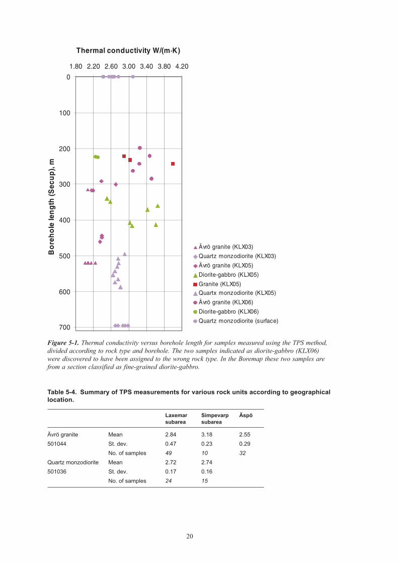
5.2.2 ResultsSummary statistics of thermal conductivity and thermal diffusivity for each rock type are presented in Table 5-2 and Table 5-� respectively. Recently acquired data from boreholes KLX0� (15 samples) /Adl-Zarrabi 2005a/; KLX05 (24 samples) /Adl-Zarrabi 2005b/ and KLX06 (7 samples) /Adl-Zarrabi 2005c/, as well as from the surface (10 samples) /Dinges 2005/ are presented in Figure 5-1. Previously produced data are described in /Sundberg et al. 2006/. While compiling and summarising the data, two samples of fine-grained diorite-gabbro (505102) from borehole KLX06 (Figure 5-1) were incorrectly assigned to diorite-gabbro (5010��) (see Table 5-2 and Table 5-�). This error, discovered shortly before going to press, is judged to have only a very slight impact on the statistical rock-type models presented in Section 5.6.
The majority of samples selected for measurement are from rock that is either unaltered or has been judged to have only faint alteration. Rocks mapped as having weak, medium or strong alteration, which comprise about 10–20% of the boreholes /SKB 2006; Boremap/, have not been sampled.

19
Table5‑2. Measuredthermalconductivity(W/(m·K))ofsamplesusingtheTPSmethod.SamplesarefromtheLaxemarsubarea(KLXboreholesandthesurface),theSimpevarpsubarea(KAVandKSHboreholes)andÄspö(boreholeKA2599G01andtheprototyperepositorytunnel).
Rockname Namecode
Samplelocation Mean St.dev Max Min Numberofsamples
Comments
Fine-grained dioritoid
501030 Boreholes KSH01A and KSH02
2.79 0.16 3.16 2.51 26 No new samples
Quartz monzodiorite
501036 Boreholes KSH01A, KAV04A, KLX03, KLX05 and surface.
2.73 0.16 3.09 2.42 39 24 new samples. Little change compared to L1.2
Ävrö granite 501044 Boreholes KAV04A, KLX02, KLX03, KLX04, KLX05, KLX06, KAV01, KA2599G01, Äspö HRL prototype tunnel,
2.81 0.42 3.76 2.01 91 20 new samples. Lower mean, higher st. dev. than in L1..2
Fine-grained granite
511058 Borehole KA2599G01 3.63 3.68 3.58 2 No new samples
Granite 501058 Borehole KLX05 3.01 3.11 2.89 3 All new samplesDiorite-gabbro¹ 501033 Borehole KLX05, KLX06. 2.94 0.55 3.65 2.25 9 All new samples
¹ Two samples of fine-grained diorite-gabbro were incorrectly assigned to diorite-gabbro.
Table5‑3. Measuredthermaldiffusivity(mm2/s)ofsamplesusingtheTPSmethod.SamplesarefromtheLaxemarsubarea(KLXboreholesandthesurface)andtheSimpevarpsubarea(KAVandKSHboreholes).
Rockname Namecode
Samplelocation Mean St.dev Numberofsamples
Comments
Fine-grained dioritoid
501030 Boreholes KSH01A, KSH02
1.28 0.16 26 No new samples
Quartz monzo-diorite
501036 Boreholes KSH01A, KAV04A, KLX03, KLX05 and surface.
1.21 0.09 39 24 new samples. Little change compared to L1.2
Ävrö granite 501044 Boreholes KAV04A, KLX02, KLX03, KLX04, KLX05, KLX06, KAV01.
1.29 0.22 59 20 new samples. Lower mean, higher st. dev. than in L1.2
Granite 501058 Borehole KLX05 1.40 3 All new samplesDiorite-gabbro¹ 501033 Borehole KLX05, KLX06. 1.19 0.20 9 All new samples
¹ Two samples of fine-grained diorite-gabbro were incorrectly assigned to diorite-gabbro.
Relative to the results presented in model version 1.2, the additional new data for rock type Ävrö granite has the effect of reducing the mean1 thermal conductivity and increasing the standard deviation. The new data for quartz monzodiorite has little effect on the summary statistics presented in version 1.2. Results for diorite-gabbro reveal a large spread in thermal conductivity values.
Table 5-4 presents data for two rock types according to geographical location. The mean thermal conductivity for Ävrö granite is lowest on Äspö and highest in Simpevarp. However, given the large variation in thermal conductivity displayed by Ävrö granite it is not possible to draw any definite conclusions regarding these apparent differences in thermal conductivity.
1 “Mean” in this case and in all subsequent cases refers to the arithmetic mean. Where the geometric mean is intended “geometric mean” is used.
20
Table5‑4. SummaryofTPSmeasurementsforvariousrockunitsaccordingtogeographicallocation.
Laxemarsubarea
Simpevarpsubarea
Äspö
Ävrö granite Mean 2.84 3.18 2.55501044 St. dev. 0.47 0.23 0.29
No. of samples 49 10 32Quartz monzodiorite Mean 2.72 2.74501036 St. dev. 0.17 0.16
No. of samples 24 15
Figure 5‑1. Thermal conductivity versus borehole length for samples measured using the TPS method, divided according to rock type and borehole. The two samples indicated as diorite-gabbro (KLX06) were discovered to have been assigned to the wrong rock type. In the Boremap these two samples are from a section classified as fine-grained diorite-gabbro.
0
100
200
300
400
500
600
700
1.80 2.20 2.60 3.00 3.40 3.80 4.20
Thermal conductivity W/(m·K)B
ore
ho
lele
ng
th(S
ecu
p),
m
Ävrö granite (KLX03)
Quartz monzodiorite (KLX03)
Ävrö granite (KLX05)
Diorite-gabbro (KLX05)
Granite (KLX05)
Quartx monzodiorite (KLX05)
Ävrö granite (KLX06)
Diorite-gabbro (KLX06)
Quartz monzodiorite (surface)

21
Surface samples of quartz monzodiorite have a lower mean thermal conductivity than samples from boreholes. A closer analysis of the surface data reveals a tendency towards lower thermal conductivity for samples taken close to the contact with Ävrö granite.
5.2.3 DeclusteringofthermalconductivitydatafordominantrocktypesSince several samples of Ävrö granite and quartz monzodiorite have been taken in groups from short, ca. 1 m, sections of borehole core, the data distributions for the rock types are not necessarily representative. This spatial clustering of sample data may produce bias in both the mean and the standard deviation. The effect of non-representative sampling can be analysed by using different declustering methods. The cell declustering approach /Isaaks and Srivastava 1989/ is used to obtain an estimate of the mean. Using this method, each spatially related group of samples (< 1 m) receives the same weight as a single isolated sample. Another method can be employed to obtain a representative estimate of the standard deviation. This is achieved by randomly selecting one sample from each group, and then calculating the standard deviation from these values. The results of declustering are presented in Table 5-5 and Table 5-6.
A comparison of the different methods for Ävrö granite reveals that declustering has little effect on the mean and standard deviation of thermal conductivity obtained using the complete data set. Given the high degree of spatial variation present within this rock type, this result seems somewhat coincidental. In conclusion, it is proposed that the mean and standard deviation most representative for Ävrö granite are 2.90 W/(m·K) and 0.46 W/(m·K). For quartz monzodiorite, a representative mean and standard deviation are estimated as 2.70 W/(m·K) and 0.17 W/(m·K), slightly different to statistics based on the complete data set.
Figure 5-2 shows the distribution of thermal conductivity values for the Ävrö granite based on a) all TPS data, and b) declustered data. In both cases, data from Laxemar and Simpevarp are included whereas Äspö data is omitted. A similar picture emerges from both histograms, i.e. at least two modes are present.
Probability plots of TPS data for quartz monzodiorite shows that the both the full data set and the declustered data set are consistent with a normal distribution (Figure 5-�).
Table5‑5. Thermalconductivity(W/(m·K))ofrocktypeÄvrögranitebasedonTPSmeasure‑ments.Comparisonofsummarystatisticscalculatedbydifferentmethods(Äspödatahasbeenexcluded).
Nodeclustering Celldeclustering Randomdeclustering
Mean 2.896 2.895 2.891St. dev. 0.456 0.446 0.460
No. of samples/data 59 26 26
Table5‑6. Thermalconductivity(W/(m·K))ofrocktypequartzmonzodioritebasedonTPSmeasurements.Comparisonofsummarystatisticscalculatedbydifferentmethods.
Nodeclustering Celldeclustering Randomdeclustering
Mean 2.725 2.699 2.709St. dev. 0.161 0.161 0.172
No. of samples/data 39 23 23

22
5.2.4 TemperaturedependenceThe temperature dependence of thermal conductivity was reported in /Sundberg et al. 2006/. The thermal conductivity decreases for the investigated rock types by on average between about 1 and 5% per 100°C temperature increase, see /Sundberg et al. 2006/.
5.3 Thermalconductivityfrommineralcomposition5.3.1 MethodThermal conductivity of rock samples can be calculated by the SCA method (Self Consistent Approximation) using mineral compositions from modal analyses and reference values of the thermal conductivity of different minerals as described in /Sundberg 1988/ and /Sundberg 200�a/.
The following data was available for calculations by the SCA-method.• Modal analyses from samples (172 in total) included in site descriptive model version 1.2 for
Laxemar /Sundberg et al. 2006/.• A total of 28 new modal analyses on samples from the surface (6 samples) and from bore-
holes KLX0�, KLX04, KLX06 (16 samples) collected as part of the geological programme /Wahlgren et al. 2005b, 2006/, in addition to samples taken close to samples for laboratory measurement of thermal properties (6 samples from KLX0�; SICADA field note no. 676)/.
Figure 5‑2. Histogram of thermal conductivity from TPS data for Ävrö granite.
Figure 5‑3. Probability plots of TPS data for quartz monzodiorite.
2�
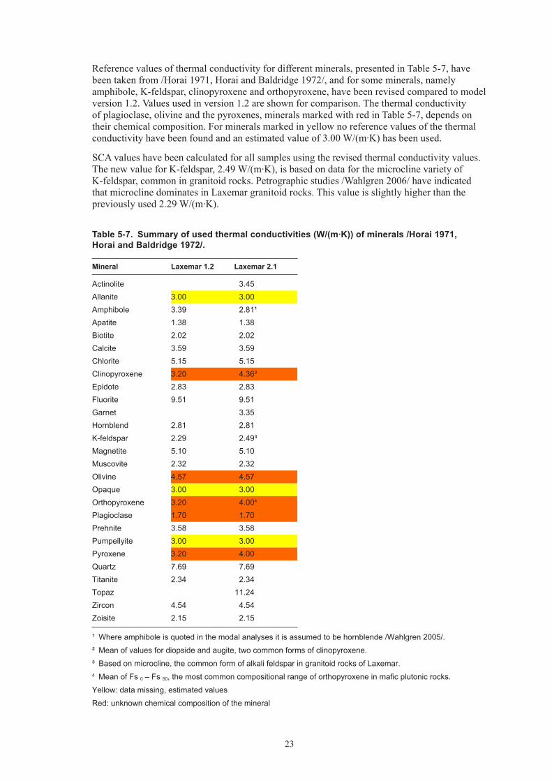
Reference values of thermal conductivity for different minerals, presented in Table 5-7, have been taken from /Horai 1971, Horai and Baldridge 1972/, and for some minerals, namely amphibole, K-feldspar, clinopyroxene and orthopyroxene, have been revised compared to model version 1.2. Values used in version 1.2 are shown for comparison. The thermal conductivity of plagioclase, olivine and the pyroxenes, minerals marked with red in Table 5-7, depends on their chemical composition. For minerals marked in yellow no reference values of the thermal conductivity have been found and an estimated value of �.00 W/(m·K) has been used.
SCA values have been calculated for all samples using the revised thermal conductivity values. The new value for K-feldspar, 2.49 W/(m·K), is based on data for the microcline variety of K-feldspar, common in granitoid rocks. Petrographic studies /Wahlgren 2006/ have indicated that microcline dominates in Laxemar granitoid rocks. This value is slightly higher than the previously used 2.29 W/(m·K).
Table5‑7. Summaryofusedthermalconductivities(W/(m·K))ofminerals/Horai1971,HoraiandBaldridge1972/.
Mineral Laxemar1.2 Laxemar2.1
Actinolite 3.45Allanite 3.00 3.00Amphibole 3.39 2.81¹Apatite 1.38 1.38Biotite 2.02 2.02Calcite 3.59 3.59Chlorite 5.15 5.15Clinopyroxene 3.20 4.36²Epidote 2.83 2.83Fluorite 9.51 9.51Garnet 3.35Hornblend 2.81 2.81K-feldspar 2.29 2.49³Magnetite 5.10 5.10Muscovite 2.32 2.32Olivine 4.57 4.57Opaque 3.00 3.00Orthopyroxene 3.20 4.004
Plagioclase 1.70 1.70Prehnite 3.58 3.58Pumpellyite 3.00 3.00Pyroxene 3.20 4.00Quartz 7.69 7.69Titanite 2.34 2.34Topaz 11.24Zircon 4.54 4.54Zoisite 2.15 2.15
¹ Where amphibole is quoted in the modal analyses it is assumed to be hornblende /Wahlgren 2005/.
² Mean of values for diopside and augite, two common forms of clinopyroxene.
³ Based on microcline, the common form of alkali feldspar in granitoid rocks of Laxemar.4 Mean of Fs 0 – Fs 50, the most common compositional range of orthopyroxene in mafic plutonic rocks.
Yellow: data missing, estimated values
Red: unknown chemical composition of the mineral

24
5.3.2 ResultsThe results of the SCA calculations from mineral composition based on all available modal analyses from Laxemar and Simpevarp subareas, and arranged according to rock type are presented in Table 5-8. The newly acquired data for Ävrö granite and quartz monzodiorite has little effect on the summary statistics presented in model version 1.2.
5.3.3 ComparisonwithmeasurementsFor several of the borehole cores on which samples have been taken for laboratory determina-tion of thermal conductivity (TPS method), sampling for modal analysis and SCA calculations has also been carried out /Sundberg et al. 2005b, 2006/. The objective is to compare determina-tions from the different methods so as to evaluate the accuracy of the SCA calculations. Six new data pairs are available, four for Ävrö granite two for quartz monzodiorite. In Table 5-9, a comparison of TPS and SCA data is presented. It should be emphasised that the samples are not exactly the same, but come from adjacent sections of the borehole. Therefore, some of the observed differences are probably a result of sampling.
The results indicate a bias in the SCA calculations for the three investigated rock types. The SCA values for quartz monzodiorite and fine-grained dioritoid are invariably lower than the corresponding TPS values. The SCA values determined for fine-grained dioritoid are based on modal analyses for which alteration products have not been taken into account, which is a departure from the procedure adopted in Simpevarp 1.2 and Laxemar 1.2. Taking all Ävrö granite samples together, the mean thermal conductivity from SCA is lower than that for TPS.
Table5‑8. Thermalconductivity(W/(m·K))calculatedfrommineralogicalcompositions(SCAmethod)fordifferentrocktypes.
Rockname Namecode Mean St.dev Max min Numberofsamples
Comment
Fine-grained dioritoid 501030 2.38 0.22 2.96 1.92 30Quartz monzodiorite 501036 2.41 0.14 2.64 2.13 28 5 new samples
Ävrö granite 501044 2.71 0.33 3.59 2.06 109 23 new samplesFine-grained diorite-gabbro 505102 2.39 0.16 2.59 2.09 10Diorite/gabbro 501033 2.28 0.13 2.50 2.05 7Fine-grained granite 511058 3.38 0.31 3.76 2.58 10Granite 501058 3.15 0.38 3.80 2.86 5¹
¹ One sample taken from outside (west of) the Laxemar subarea.
Table5‑9. ComparisonofthermalconductivityofdifferentrocktypescalculatedfrommineralogicalcompositionsbytheSCAmethodandmeasuredwiththeTPSmethod.SamplesfromboththeLaxemarandSimpevarpsubareas.
Method Fine‑graineddioritoid(501030)5samples
Mean λ, (W/(m·K))
Quartzmonzodiorite(501036)5samples
Mean λ, (W/(m·K))
Ävrögranite(501044),all17samples
Mean λ, (W/(m·K))
Ävrögranite,6samples(<2.7W/(m·K))
Mean λ, (W/(m·K))
Ävrögranite,11samples(>3.0W/(m·K))
Mean λ, (W/(m·K))
Calculated (SCA) 2.481 2.361 2.74 2.32 2.94Measured (TPS) 2.85 2.67 2.88 2.32 3.16Diff. (SCA -TPS)/TPS –13.0% –11.9% –4.9% 0.4% –6.9%
1 No correction for sericitisation and chloritization made.

25
However, an interesting picture emerges on plotting SCA values against TPS values for this rock type. Figure 5-4 shows that for high conductivity samples (> �.0 W/(m·K)) of Ävrö granite there is poor agreement between the two data sets (SCA consistently underestimates the “true” thermal conductivity) whereas for low conductivity samples (< 2.7 W/(m·K)) no obvious bias is apparent.
Possible explanations for the systematic bias observed in the SCA calculations are alteration products not being considered, variable anorthite contents of plagioclase, uncertainties regarding the reference values assigned to minerals, and errors associated with point-counting method. For a discussion of these possible alternatives, see /Sundberg et al. 2006/. Several of both low conductivity and high conductivity Ävrö granite samples exhibit some degree of alteration, which suggests that alteration is not the sole factor producing the bias observed for the high-conductivity samples. A possible contributing factor is the thermal conductivity value assigned to plagioclase, which has been shown to vary depending on the anorthite content. Plagioclase in the more quartz-rich Ärvö granite may have a lower anorthite content than in the quartz poor varieties. However, this has not been demonstrated, so the same value for all plagioclase has been used.
The SCA data for Ävrö granite was corrected in accordance with the bias noted in the table above. Samples with conductivities higher than 2.7 W/(m·K) have been adjusted by a factor of 1.07. The cut-off point of 2.7 W/(m·K) was chosen based on the results shown in Figure 5-4. This cut-off corresponds well with a natural break in the compositional range as shown in the histogram in Figure 5-5. A histogram of the corrected SCA values for Ävrö granite is also given in Figure 5-5. With or without this correction, the distribution exhibits a marked bimodality. The corrected distribution displays a close correspondence with the distribution of TPS values, see Figure 5-2.
Figure 5‑4. TPS versus SCA data for the “same” samples.

26
5.3.4 RelationshipbetweenthermalconductivityandigneousrocktypeÄvrö granite displays a wide compositional range. Based on mineralogy and geochemical composition, two distinct populations of Ävrö granite have been distinguished, one richer in quartz (granite to granodiorite), the other with a lower quartz content (quartz monzodioritic) /SKB 2006/. This broadly bimodal distribution is also displayed by thermal conductivity values determined by the TPS and SCA methods, Figure 5-2 and Figure 5-5. To further investigate the relationship between thermal conductivity and mineralogy for some important rock types, Ävrö granite in particular, Streckeisen plots have been used.
There is a clear relationship between thermal conductivity (determined from TPS and from mineral composition) and plutonic rock type as defined by the Streckeisen classification system, Figure 5-6 and Figure 5-7. Ävrö granite with granite to granodiorite composition typically have thermal conductivities greater than 2.9 W/(m·K). Varieties with quartz monzodioritic and quartz diorite composition have thermal conductivities lower than 2.7 W/(m·K). Quartz diorites have particularly low values (< 2.� W/(m·K)).
Figure 5‑5. Histograms of SCA data for Ävrö granite before and after correction for bias.
Figure 5‑6. QAP modal classification of Ävrö granite and quartz monzodiorite (QMD) (both from Laxemar and Simpevarp subareas), colour coded according to thermal conductivity (TPS method). Classification according to /Streckeisen 1976/.

27
Rock type quartz monzodiorite (5010�6) falls mainly in the quartz monzodiorite field and less commonly in the quartz diorite field /SKB 2006/. Three samples with quartz monzodiorite composition have thermal conductivities of about 2.8 W/(m·K), whereas quartz diorite samples have values of about 2.5 W/(m·K). Quartz monzodiorite, therefore, differs from Ävrö granite in having higher thermal conductivity values (2.5–2.9 W/(m·K)) for the same rock type as defined by /Streckeisen 1976/. The most plausible explanation for this is that quartz monzodiorite has a higher mafic mineral content, comprising both biotite and amphibole (hornblende). Hornblende has a thermal conductivity of about 2.8 W/(m·K) /Horai 1971/, which is higher than for feldspars. Furthermore, because of the high mafic mineral content, chlorite, with a thermal conductivity of about 5 W/(m·K), is probably more plentiful, it being a common alteration product of mafic minerals.
Diorite-gabbro shows a wide range in thermal conductivities (from 2.2 to �.6 W/(m·K)). However, differences in mineralogy are not obvious on a Streckeisen diagram because of the low content of quartz and alkali-feldspar typical of such rock types. A plausible explanation for the observed variation in conductivity is the differing proportions of plagioclase and mafic minerals, a hypothesis supported by the observed relationship between density and thermal conductivity, see Section 5.4. Alteration of biotite and amphibole to chlorite may also be a controlling factor. More modal analysis data for diorite-gabbro is required to describe the relationship between mineralogy and thermal conductivity more precisely.
Figure 5‑7. QAP modal classification according to /Streckeisen 1976/ of Ävrö granite, colour coded according to thermal conductivity (SCA method) from samples from Laxemar subarea. It should be noted that samples with conductivities higher than 2.7 W/(m·K) have been corrected to account for the observed bias in the SCA data.
28
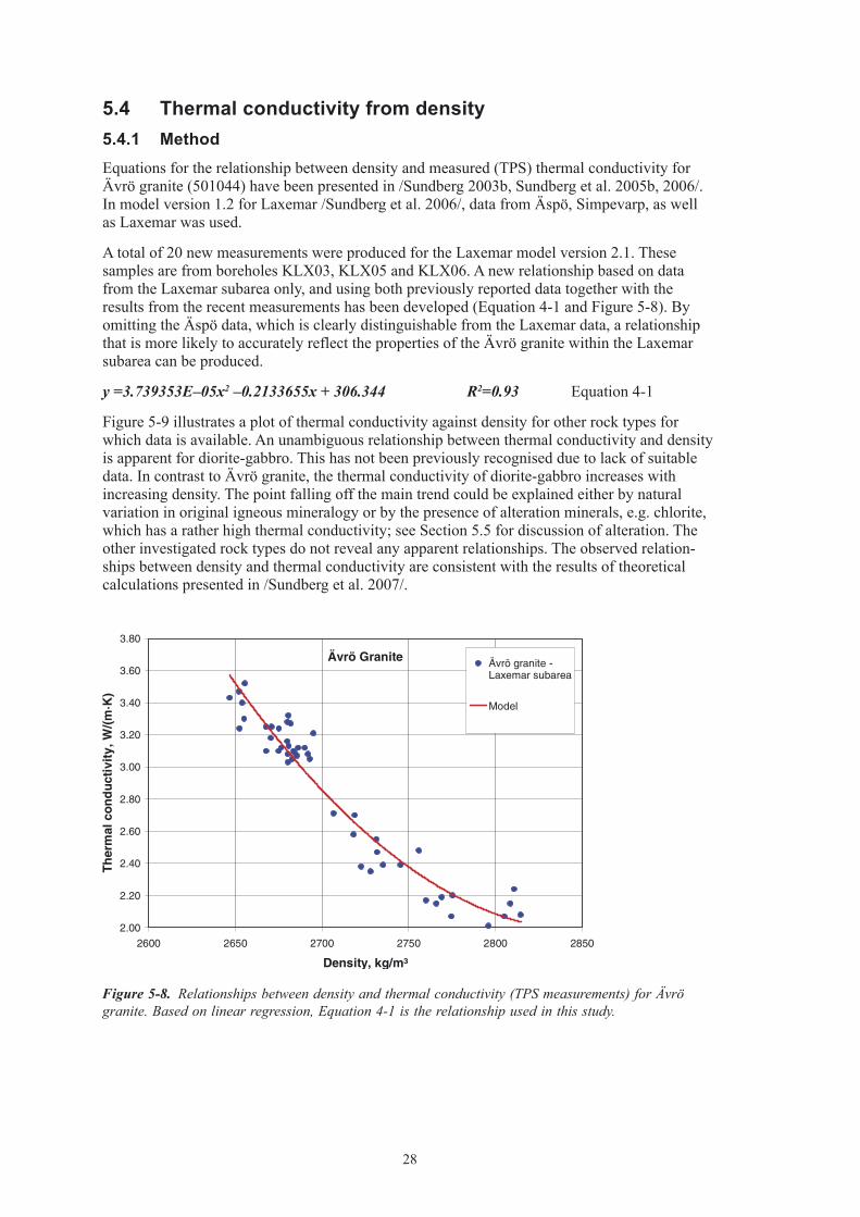
5.4 Thermalconductivityfromdensity5.4.1 MethodEquations for the relationship between density and measured (TPS) thermal conductivity for Ävrö granite (501044) have been presented in /Sundberg 200�b, Sundberg et al. 2005b, 2006/. In model version 1.2 for Laxemar /Sundberg et al. 2006/, data from Äspö, Simpevarp, as well as Laxemar was used.
A total of 20 new measurements were produced for the Laxemar model version 2.1. These samples are from boreholes KLX0�, KLX05 and KLX06. A new relationship based on data from the Laxemar subarea only, and using both previously reported data together with the results from the recent measurements has been developed (Equation 4-1 and Figure 5-8). By omitting the Äspö data, which is clearly distinguishable from the Laxemar data, a relationship that is more likely to accurately reflect the properties of the Ävrö granite within the Laxemar subarea can be produced.
y =3.739353E–05x2 –0.2133655x + 306.344 R2=0.93 Equation 4-1
Figure 5-9 illustrates a plot of thermal conductivity against density for other rock types for which data is available. An unambiguous relationship between thermal conductivity and density is apparent for diorite-gabbro. This has not been previously recognised due to lack of suitable data. In contrast to Ävrö granite, the thermal conductivity of diorite-gabbro increases with increasing density. The point falling off the main trend could be explained either by natural variation in original igneous mineralogy or by the presence of alteration minerals, e.g. chlorite, which has a rather high thermal conductivity; see Section 5.5 for discussion of alteration. The other investigated rock types do not reveal any apparent relationships. The observed relation-ships between density and thermal conductivity are consistent with the results of theoretical calculations presented in /Sundberg et al. 2007/.
Figure 5‑8. Relationships between density and thermal conductivity (TPS measurements) for Ävrö granite. Based on linear regression, Equation 4-1 is the relationship used in this study.

29
5.4.2 ResultsBased on the relationship between density and thermal conductivity derived for Ävrö granite, as explained in Section 5.4.1, density values given by the density loggings of boreholes KLX01, KLX02, KLX0�, KLX04, KLX05 and KLX06 were used to deterministically assign a thermal conductivity value to each logged decimetre section of Ävrö granite. Density loggings plotted against rock type (occurrences > 1 m) for boreholes KLX01–04 are illustrated in /Sundberg et al. 2006/.
Density logging data for all boreholes were re-sampled, calibrated and filtered /Mattsson 2004, 2005, Mattsson and Keisu 2005, Mattsson et al. 2005/. The calibration procedure used is identical to that used in model version Laxemar 1.2. Noise levels for KLX05 and KLX06 are 14 kg/m� /Mattsson and Keisu 2005/ and 22 kg/m� /Mattsson 2005/ respectively. Noise levels are above the recommended levels (�–5 kg/m�) for all density logs with the exception of the logs for KLX01 /Mattsson et al. 2005/. Noise levels for KLX02, at 64 kg/m�, are particularly high /Mattsson 2004/.
For the purposes of modelling thermal conductivity from density loggings, it is assumed that the established relationship, Equation 4-1, is valid within the density interval 2,625–2,850 kg/m³. This range corresponds to the thermal conductivity interval 1.98–�.9� W/(m·K), i.e. slightly outside the interval of measured data. The extreme high values of thermal conductivity produced are purely an effect of the considerable random noise in the density loggings. The influence of these extreme values effectively diminishes as a consequence of upscaling, since the regression curve is close to linear over a limited density interval. Table 5-10 summarises the results of the measurements for each borehole.
The frequency histograms in Figure 5-10 display the distribution of thermal conductivity values for Ävrö granite calculated from density loggings for all boreholes at two different scales, 0.1 m and 1m. The existence of more than one mode becomes apparent on scaling up to 1 m. At this scale, the distribution of thermal conductivity values contains two modes, one at 2.5 W/(m·K) and one at �.05 W/(m·K). However, others modes may be present. This seemingly bimodal distribution is also evident in both the TPS and SCA data sets for Ävrö granite.
Figure 5‑9. Relationships between density and thermal conductivity for five rock types.

�0
Table5‑10. SummaryofdensityloggingofÄvrögraniteperborehole.
Borehole %Ävrögraniteinborehole
No.ofmeasurementswithindensityinterval2,625–2,850kg/m³
%measure‑mentsexcluded(outsidemodelinterval)
Loggedboreholeinterval,m
Thermalconductivity,W/(m·K)–Mean(st.dev.)0.1mscale
Thermalconductivity,W/(m·K)–Mean(st.dev.)1mscale
%below/above2.85W/(m·K),1mscale
KLX01 80.03 5,533 1.3% 1.0–701.6 m 2.58 (0.25) 2.58 (0.23) 91/9KLX02 70.88 5,584 8.9% 201.5–1,004.9 m 2.92 (0.47) 2.90 (0.28) 40/60KLX03 54.18 4,827 0.8% 101.8–999.9 m 2.38 (0.22) 2.38 (0.16) 98/2KLX04 72.23 6,344 1.2% 101.6–990.2 m 2.92 (0.37) 2.92 (0.31) 32/68KLX05 15.95 1,373 2.8% 108.4–994.3 2.78 (0.44) 2.76 (0.36) 59/41KLX06 55.6 4,720 4.4% 101.90–989.80 2.82 (0.40) 2.80 (0.33) 65/35All boreholes 28,381 2.74 (0.41) 2.73 (0.35) 63/37
Figure 5‑10. Histograms of thermal conductivity for Ävrö granite calculated from density loggings for boreholes KLX01 – KLX06.
�1
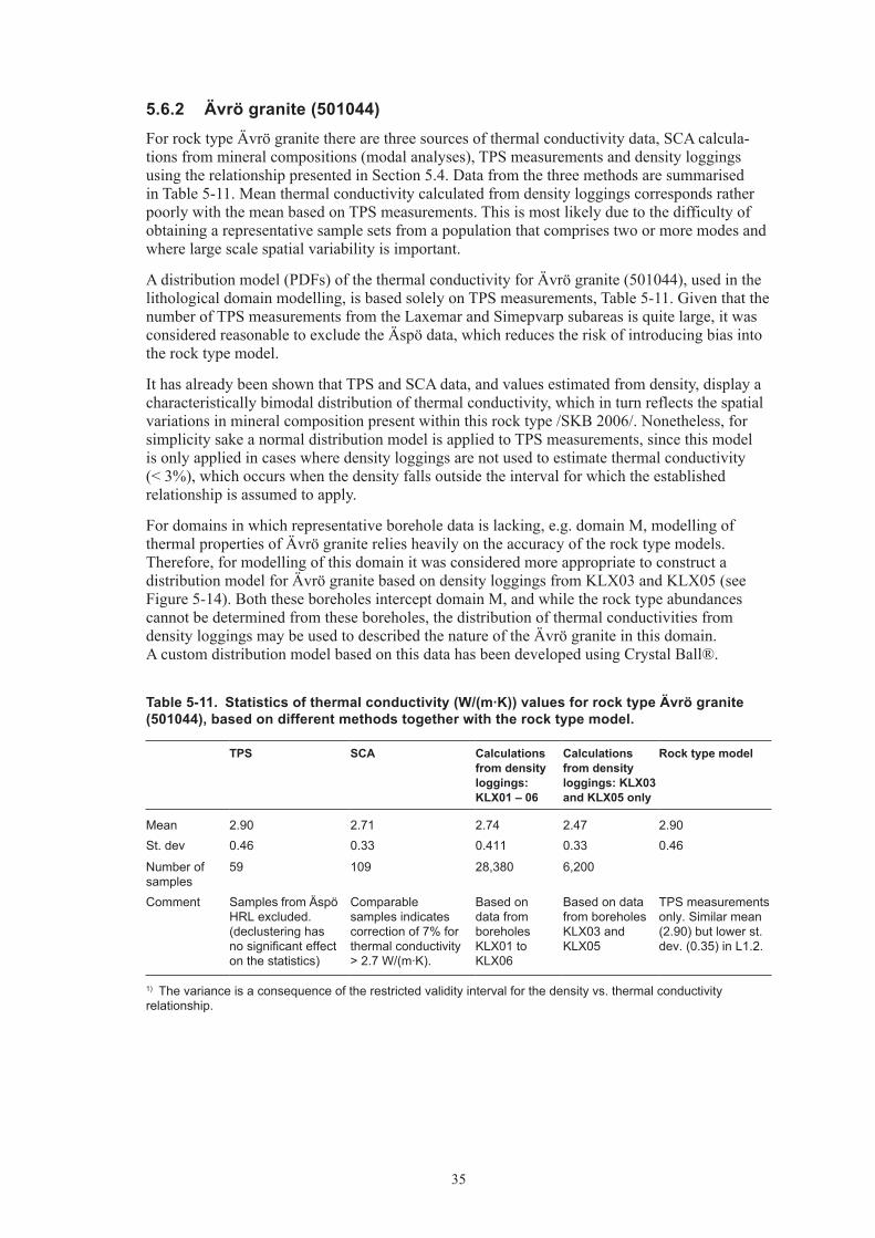
A comparison of the distributions in the individual boreholes reveals large differences, as reflected by the proportions of the low (< 2.85 W/(m·K)) and high (> 2.85 W/(m·K)) modes. KLX01 and KLX0� are dominated by low conductivities whereas KLX02 and KLX04 have a predominance of high conductivity Ävrö granite. KLX05 and KLX06 comprise large proportions of both modes, Table 5-10. The overall proportion of the different modes is highly dependent on the location of the boreholes used, and may not accurately represent the rock mass within the Laxemar subarea.
The mean and standard deviation of thermal conductivity for Ävrö granite based on density log-gings from all boreholes (2.74 W/(m·K) and 0.41 W/(m·K) respectively) are significantly differ-ent than the results presented in Laxemar model version 1.2 (2.88 W/(m·K) and 0.�� W/(m·K) respectively). This is in part due to the availability of data from additional boreholes, and in part a result of the revised thermal conductivity – density model.
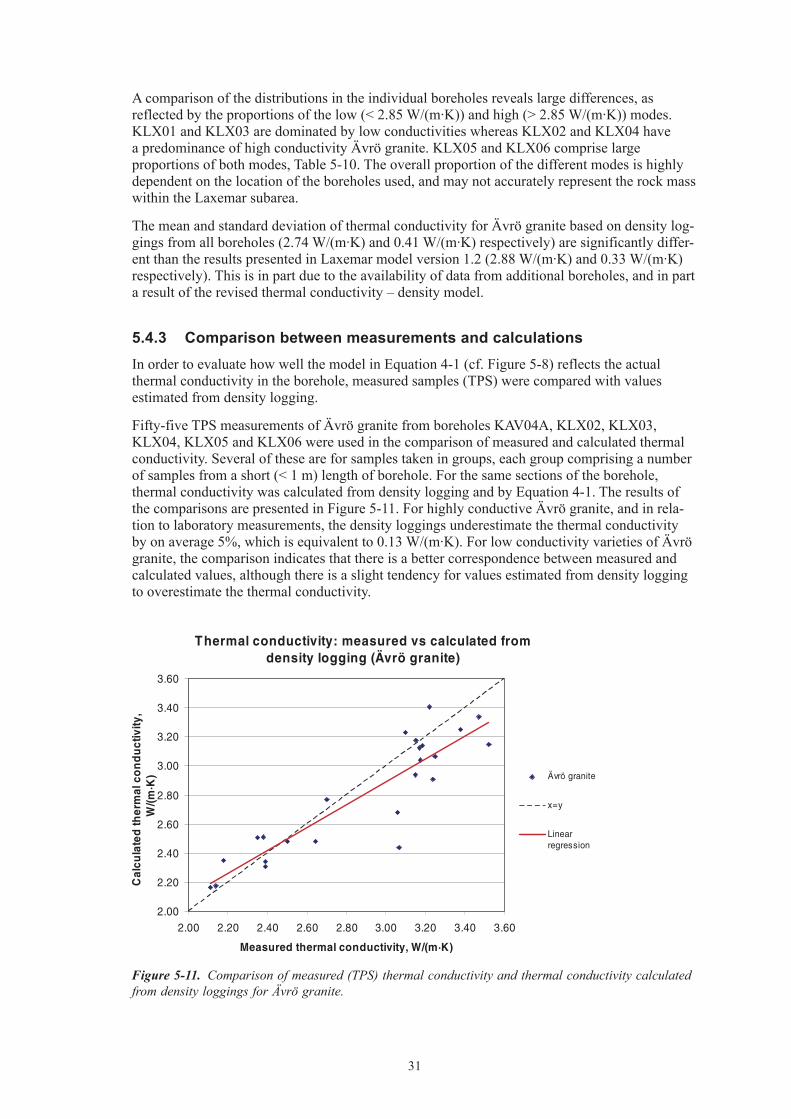
5.4.3 ComparisonbetweenmeasurementsandcalculationsIn order to evaluate how well the model in Equation 4-1 (cf. Figure 5-8) reflects the actual thermal conductivity in the borehole, measured samples (TPS) were compared with values estimated from density logging.
Fifty-five TPS measurements of Ävrö granite from boreholes KAV04A, KLX02, KLX0�, KLX04, KLX05 and KLX06 were used in the comparison of measured and calculated thermal conductivity. Several of these are for samples taken in groups, each group comprising a number of samples from a short (< 1 m) length of borehole. For the same sections of the borehole, thermal conductivity was calculated from density logging and by Equation 4-1. The results of the comparisons are presented in Figure 5-11. For highly conductive Ävrö granite, and in rela-tion to laboratory measurements, the density loggings underestimate the thermal conductivity by on average 5%, which is equivalent to 0.1� W/(m·K). For low conductivity varieties of Ävrö granite, the comparison indicates that there is a better correspondence between measured and calculated values, although there is a slight tendency for values estimated from density logging to overestimate the thermal conductivity.
Figure 5‑11. Comparison of measured (TPS) thermal conductivity and thermal conductivity calculated from density loggings for Ävrö granite.

�2
Direct density measurements on samples, and density loggings from the corresponding borehole interval have also been compared, Figure 5-12. The logged density data for KLX02 displays a high degree of dispersion compared to measured values. The poor fit may be due to the high noise in the density loggings for this borehole /Mattsson 2004/. The average difference in density calculated by the two separate methods is 0.�6%, implying that the logging data is overestimating density by about 10 kg/m�. In terms of thermal conductivity this is equivalent to underestimation of thermal conductivity by about 0.1 W/(m·K).
5.5 AlterationAlteration observed in the Laxemar borehole cores includes oxidation, saussuritization epidotization, chloritization, sericitization and silicification. Rock affected by alteration comprises about 25% of the boreholes KLX01 to KLX04 /SKB 2006/. Most alteration is faint to weak in character. KLX01, KLX02 and KLX04 are dominated by oxidation, while KLX0� has an important component of saussuritization. In KLX05 and KLX06 about 15% and 25% of the boreholes respectively show weak, medium or strong alteration; in KLX05 both saussuritization and oxidation are important, whereas in KLX06 oxidation dominates, but saussuritization is also present (Sicada, Boremap). Alteration is not limited to particular rock types.
Hydrothermal alteration has given rise to red staining and saussuritization. The most apparent alteration in the Laxemar subarea is the extensive red-staining of the host rock along and around fractures and interpreted deformation zones, which is in contrast to the Simpevarp subarea where the red staining also affects the interiors of rock volumes between prominent mesoscopic fractures /SKB 2006/. The red-staining of the wall rock is interpreted as an effect of hydrothermal alteration/oxidation, which has resulted in alteration of plagioclase to albite and K-feldspar, decomposition of biotite to chlorite and oxidation of Fe(II) to form hematite, mainly present as micrograins in secondary K-feldspar and albite giving the red colour /SKB 2006/. Other widespread alterations are the chloritization of biotite and saussuritization/sericiti-zation of plagioclase and more rarely of K-feldspar /Drake and Tullborg 2005/. It is important to note that alteration extends beyond the zone of visible alteration, e.g. red-staining. For example, outside the visibly altered zones, alteration phenomena are still apparent in thin sections, for example chloritization of biotite /Drake and Tullborg 2005/.
Figure 5‑12. Comparison of measured density and logged density for Ävrö granite.

��
The samples from the Laxemar and Simpevarp subareas on which TPS measurements were performed were generally taken from borehole cores showing little (“faint”) or no alteration. An exception to this is a sample of Ävrö granite from KLX06 (secup 221.�1 m), described in Boremap mapping as having “weak” oxidation and illustrated in Figure 5-1�. This sample yielded a thermal conductivity of �.47 W/(m·K) measured using the TPS method, which is at the higher end of the range of thermal conductivity values for this rock type.
Similar alteration features to those described above were recorded in granite on the nearby island of Äspö by /Eliasson 199�/. Investigations of thermal properties at Äspö HRL for a number of samples indicate that the mean thermal conductivity of altered “Äspö diorite” (Ävrö granite of quartz monzodioritic composition) is higher than that of fresh “Äspö diorite” /Sundberg 200�b/. Four altered samples gave a mean of 2.81 whereas 12 fresh samples gave a mean of 2.49, a difference of about 1�%. The alteration in this case was characterised by the replacement of biotite by chlorite. Chlorite has a higher thermal conductivity than biotite; 5.1 W/(m·K) versus 2.0 W/(m·K) /Horai 1971/. Furthermore, the density of the altered samples is lower than that of the fresh varieties. One altered sample yielded a thermal conductivity value of �.11 /Sundberg 2002/, unusually high for the quartz poor variety of Ävrö granite. This sample consisted of 14% chlorite, and plagioclase had an albitic composition, typical mineralogy of altered rocks /Sundberg 2002/. These mineralogical changes can largely explain the high thermal conductivity value for the rock sample.
Figure 5‑13. Two core samples of Ävrö granite from KLX06 used for measuring thermal properties by the TPS method /Adl-Zarrabi 2005c/. Sample 02 (secup: 221.31 m) in the top photo is from a section described in the Boremap as having weak alteration, whereas for sample 04 (secup: 263.53 m) in the bottom photo no alteration was noted in the Boremap. Note the more obvious red colouration indicative of oxidation in sample 02.

�4
The samples on which SCA calculations were based were generally taken with the purpose of characterising the unaltered rock. However, modal analysis data exists for a number of altered samples investigated by /Drake and Tullborg 2006/. SCA calculations for these samples have as yet not been performed, but could be performed to investigate the effect of alteration on thermal conductivity.
Summing up, it can be stated that samples for which thermal properties have been determined either by measurement or from mineral composition are, with only some exceptions, taken from cores that are considered to be unaltered. Therefore, a relatively large part of the rock mass is not represented by the available TPS or SCA data. However, it should be pointed out that even samples from core which do not show obvious signs of alteration (e.g. absence of red-staining) have been shown in thin section analysis to display partial replacement of biotite by chlorite /Drake and Tullborg 2006/ and partial sericitisation of plagioclase /Sundberg et al. 2005b/. It is also of relevance that the rock mass in at least the larger deformation zones (zones of intense fracturing where alteration is most intense) will not be exploited for the nuclear waste repository.
Many of the minerals associated with the forms of alteration described above, such as K-feld-spar, albite, sericite, epidote, prehnite, chlorite, etc, have thermal conductivities that are similar to or higher than their parent minerals, for example, plagioclase, biotite, etc. Theoretically, these mineralogical changes should then produce higher rock thermal conductivities.
5.6 Statisticalrocktypemodelsofthermalconductivity5.6.1 MethodThe most reliable data for thermal conductivity is provided by TPS measurements. However, due to the limited number of samples and the sample selection procedure, the data sets may not be representative of the rock type. Samples on which SCA calculations are based have a larger spatial distribution in the rock mass.
Rock type models (Probability Density Functions, PDFs) of thermal conductivity have, with the exception of Ävrö granite and quartz monzodiorite, been produced by combining the available data from TPS measurements and SCA calculations from mineral composition. For one rock type, fine-grained diorite-gabbro, only SCA calculations are available. The SCA calculations of rock type fine-grained dioritoid (5010�0) have been corrected by a factor of 1.10 in order to reduce the effect of a potential bias in the SCA calculations according to Table 5-9. SCA data for quartz monzodiorite (5010�6) and Ävrö granite (501044) have not been used in the construction of rock type models. Because of the availability of additional TPS measurements, it has been decided to exclude the more uncertain SCA calculations from the input to the respective rock models.
The rock type models are used to model thermal properties for lithological domains, see Chapter 6. In modelling thermal conductivity using borehole data, rock types are generally assumed to be characterised by normal (Gaussian) PDFs. For Ävrö granite this assumption is unlikely to hold true. The available data for this rock type displays a bimodal distribution. However, this is only of minor importance in the modelling work which follows, since thermal conductivities for this rock type are generally calculated from density loggings, the PDF being applied to less than �% of the Ävrö granite in the boreholes. When borehole data is not available for domain modelling, Monte Carlo simulation is used instead. In the case of domain RSMM, custom distributions for two rock types, namely Ävrö granite and diorite-gabbro have been developed.
�5
5.6.2 Ävrögranite(501044)For rock type Ävrö granite there are three sources of thermal conductivity data, SCA calcula-tions from mineral compositions (modal analyses), TPS measurements and density loggings using the relationship presented in Section 5.4. Data from the three methods are summarised in Table 5-11. Mean thermal conductivity calculated from density loggings corresponds rather poorly with the mean based on TPS measurements. This is most likely due to the difficulty of obtaining a representative sample sets from a population that comprises two or more modes and where large scale spatial variability is important.
A distribution model (PDFs) of the thermal conductivity for Ävrö granite (501044), used in the lithological domain modelling, is based solely on TPS measurements, Table 5-11. Given that the number of TPS measurements from the Laxemar and Simepvarp subareas is quite large, it was considered reasonable to exclude the Äspö data, which reduces the risk of introducing bias into the rock type model.
It has already been shown that TPS and SCA data, and values estimated from density, display a characteristically bimodal distribution of thermal conductivity, which in turn reflects the spatial variations in mineral composition present within this rock type /SKB 2006/. Nonetheless, for simplicity sake a normal distribution model is applied to TPS measurements, since this model is only applied in cases where density loggings are not used to estimate thermal conductivity (< �%), which occurs when the density falls outside the interval for which the established relationship is assumed to apply.
For domains in which representative borehole data is lacking, e.g. domain M, modelling of thermal properties of Ävrö granite relies heavily on the accuracy of the rock type models. Therefore, for modelling of this domain it was considered more appropriate to construct a distribution model for Ävrö granite based on density loggings from KLX0� and KLX05 (see Figure 5-14). Both these boreholes intercept domain M, and while the rock type abundances cannot be determined from these boreholes, the distribution of thermal conductivities from density loggings may be used to described the nature of the Ävrö granite in this domain. A custom distribution model based on this data has been developed using Crystal Ball®.
Table5‑11. Statisticsofthermalconductivity(W/(m·K))valuesforrocktypeÄvrögranite(501044),basedondifferentmethodstogetherwiththerocktypemodel.
TPS SCA Calculationsfromdensityloggings:KLX01–06
Calculationsfromdensityloggings:KLX03andKLX05only
Rocktypemodel
Mean 2.90 2.71 2.74 2.47 2.90St. dev 0.46 0.33 0.411 0.33 0.46
Number of samples
59 109 28,380 6,200
Comment Samples from Äspö HRL excluded. (declustering has no significant effect on the statistics)
Comparable samples indicates correction of 7% for thermal conductivity > 2.7 W/(m·K).
Based on data from boreholes KLX01 to KLX06
Based on data from boreholes KLX03 and KLX05
TPS measurements only. Similar mean (2.90) but lower st. dev. (0.35) in L1.2.
1) The variance is a consequence of the restricted validity interval for the density vs. thermal conductivity relationship.

�6
5.6.3 Quartzmonzodiorite(501036)For rock type quartz monzodiorite (5010�6) there are two sources of thermal conductivity data, SCA calculations based on mineral composition and TPS measurements. Data from the two methods are summarised in Table 5-12. Because of the relatively large number of TPS values, the more uncertain SCA data has not been used to construct the rock type model. On probability plots, data from the TPS method correspond well with a normal distribution, both with and without declustering, see Figure 5-�. A rock type model of thermal conductivity used in the lithological domain modelling is based on declustered TPS data, see Table 5-12.
Table5‑12. Distributionsofthermalconductivity(W/(m·K))forrocktypequartzmonzodior‑ite(501036),basedondifferentmethodstogetherwiththerocktypemodel.
TPSmeasurements
Calculationsfrommineralcomposition
Rocktypemodel
Mean 2.70 2.41 2.70St. dev 0.17 0.14 0.17Number of samples 39 28Comment Declustered
dataComparable samples (5) indicate difference of 12%
TPS measurements only
5.6.4 Fine‑graineddioritoid(501030)For rock type fine-grained dioritoid (5010�0) there are two sources of thermal conductivity data, SCA calculations and TPS measurements. Data from the two methods are summarised in Table 5-1�. No new data is available for this rock type. The SCA calculations have produced slightly different results compared to those reported in model version 1.2, because of revised mineral conductivities, as well as the omission of one sample previously assigned incorrectly to this rock type. All data is derived from the Simpevarp subarea. As can be seen in Table 5-1�, the two methods result in different mean values and variances.
Figure 5‑14. Histogram of thermal conductivities for Ävrö granite based on density loggings from KLX03 and KLX05.

�7
A rock type model of thermal conductivity for fine-grained dioritoid, used in the lithological domain modelling, has been constructed by combining both TPS measurements and SCA calculations. The SCA calculations have in this case been corrected by a factor 1.10, which in Section 5.�.� has been shown as the approximate difference between the two methods for this particular rock type. The combined data from TPS measurements and corrected SCA calcula-tions have, using probability plots, been shown to correspond well with a normal distribution, see Figure 5-15. Taken separately, data from both the TPS method and the SCA methods have also been shown to be normal distributed, see Figure 5-15.
Table5‑13. Twodifferentdistributionsofthermalconductivity(W/(m·K))forrocktypefine‑graineddioritoid(501030)basedondifferentmethodstogetherwiththerocktypemodel.
TPSmeasurements
Calculationsfrommineralcomposition
Rocktypemodel
Mean 2.79 2.36 2.69St. dev 0.16 0.23 0.23
Number of samples 26 25Comment Comparable sample
indicate correction +13%TPS measurements and calculations from mineral composition combined.
Figure 5‑15. Probability plots (normal distributions) of thermal conductivity for rock type fine-grained dioritoid (501030). SCA calculations have been corrected by a factor of 1.10.

�8
5.6.5 Diorite‑gabbro(501033)For rock type diorite-gabbro (5010��) there are two sources of thermal conductivity data, SCA calculations and TPS measurements. Data from the two methods, summarised in Table 5-14, result in different means and variances. The main difference between the two data sets is the wide spread in values displayed by the TPS data and the narrow range of values shown by the SCA data. This is unlikely to be solely an effect of a bias associated with the SCA method, similar to that observed in rock types quartz monzodiorite and fine-grained dioritoid. An investigation of the density loggings of the borehole sections comprising diorite-gabbro indicates large-scale spatial variation in the density of this rock type. Since there would appear to be a correlation between density and thermal conductivity, see Figure 5-9, then spatial variation in thermal conductivity is also to be expected. Although density varies from 2,860 to �,020 kg/m�, any particular borehole section has a significantly more restricted density range. In KLX05, some borehole sections have densities of about 2,900 kg/m�, whereas other sections have densities of about �,000 kg/m�. In other words, there is evidence of the existence of more than one compositional type of diorite-gabbro. The abundance of each variety can be interpreted from borehole density logging. Given the existence of two or more compositional varieties of diorite-gabbro, a normal or lognormal distributed range of thermal conductivity values would not be expected.
A rock type model of the thermal conductivity for diorite-gabbro, used in the lithological domain modelling, has been constructed from a combination of both TPS measurements and SCA calculations. Comparative data is not available so no correction has been made to the SCA values. The combined data from TPS measurements and SCA calculations can, using probability plots, be shown not to correspond to a normal or lognormal distribution, although, taken separately, data from both the TPS method and the SCA methods may be normally distributed, see Figure 5-16. For domains in which diorite-gabbro comprises only a small proportion of the rock volume, and for which the choice of distribution model is not very critical, a normal distribution model has, for simplicity sake, been employed.
However, fitting a standard distribution to such data is not appropriate for modelling of domains E and M, both of which comprise large fractions of diorite-gabbro. Instead, a custom distribu-tion (Figure 5-17) has been created using Crystal Ball® for use in Monte Carlo simulation. The model takes into consideration the values obtained from both TPS and SCA data, but also the proportion of different compositional varieties as indicated by the density loggings. The variety with low thermal conductivities (low density) is considered to be the most abundant. There are obviously large uncertainties associated with such a model but it is nevertheless considered to be an improvement on the normal distribution model, which because of the high standard deviation yields unreasonably low thermal conductivity values. While the mean of the custom model is the same as that calculated from the data set, the variance is somewhat less.
Table5‑14. Twodifferentdistributionsofthermalconductivity(W/(m·K))forrocktypediorite‑gabbro(501033)basedondifferentmethodstogetherwiththerocktypemodel.
TPSmeasurements
Calculationsfrommineralcomposition
Rocktypemodel
Mean 2.94 2.28 2.65St. dev 0.55 0.13 0.53Number of samples 9 7Comment TPS measurements and calculations
from mineral composition combined.

�9
5.6.6 Otherrocktypes(505102,501058and511058)For rock types other than Ävrö granite (501044), quartz monzodiorite (5010�6), and fine-grained dioritoid (5010�0), thermal conductivity data is still rather limited. In the case of fine-grained diorite-gabbro only SCA calculations are available. In Figure 5-18 probability plots (normal distributions) of fine-grained diorite-gabbro (505102), granite (501058) and fine-grained granite (511058) are presented. The presence of outliers in the data sets of two rock types means that good fits to normal (or lognormal) distributions are not found. As mentioned above, there is greater uncertainty associated with the SCA data (especially some of the older data from which the outliers are derived). Therefore, normal distributions cannot be ruled out at this stage, and are adopted here for the rock type models. More data, particularly TPS data, is required to describe the nature of the data distributions more reliably.
Figure 5‑16. Probability plots (normal distributions) of thermal conductivity for rock type diorite-gabbro (501033).
Figure 5‑17. Custom distribution model of thermal conductivity for rock type diorite-gabbro (501033).
.000
.323
.647
.970
1.293
1.95 2.44 2.93 3.41 3.90
Mean = 2.65

40
5.6.7 SummaryofrocktypemodelsIn Table 5-15 the model properties for the different investigated rock types are summarized. For rock types 501044, 5010�6, 5010�0 and 501058, there is better representativity in the underlying data and thus a higher degree of confidence in the rock type models compared with model version 1.2. For 5010��, although several TPS measurements have become available, there are still large uncertainties remaining. While compiling and summarising the data, two TPS measurements of fine-grained diorite-gabbro (505102) from KLX06 (Figure 5-1) were incorrectly assigned to diorite-gabbro (5010��) (see Table 5-2 and Table 5-�). This error, discovered shortly before going to press, is judged to have only a very slight impact on the statistical rock-type models presented here.
Table5‑15. Modelpropertiesofthermalconductivity(W/(m·K))dividedbyrocktype.Allrocktypemodelsarebasedonnormal(Gaussian)distributions(PDFs).
Rockname(namecode)
Samples Mean St.dev Max Min No.ofsamples
L1.2–meanandstddev¹
Comment
Ävrö granite (501044)
TPS 2.90 0.46 3.76 2.01 59 2.90 (0.35) Äspö data excluded
Quartz monzodiorite (501036)
TPS 2.70 0.17 3.09 2.42 39 2.69 (0.28)
Fine-grained dioritoid (501030)
TPS+1.1·SCA 2.69 0.23 3.26 2.11 26 2.71 (0.30) All data from Simpevarp subarea
Fine-grained granite (511058)
TPS+SCA 3.42 0.30 3.76 2.57 12 3.33 (0.31)
Fine-grained diorite-gabbro (505102)
SCA 2.39 0.16 2.59 2.09 10 2.57 (0.23)
Diorite-gabbro (501033) ²
TPS+SCA 2.65 0.53 3.65 2.05 16 2.41 (0.22) Significant change in mean and standard deviation. Custom model used for domain E and M.
Figure 5‑18. Probability plots (normal distributions) of thermal conductivity for rock types fine-grained diorite-gabbro (505102), granite (501058) and fine-grained granite (511058).
41
Rockname(namecode)
Samples Mean St.dev Max Min No.ofsamples
L1.2–meanandstddev¹
Comment
Granite (501058)
TPS+SCA 3.10 0.30 3.80 2.86 8 2.59 (0.65) Significant change in mean and standard deviation.
Pegmatite (501061)
TPS+SCA 3.31 0.48 Data from /Sundberg 1988/
¹ Site descriptive model, Laxemar 1.2 /Sundberg et al. 2006/. ² Two samples of fine-grained diorite-gabbro were incorrectly assigned to diorite-gabbro.
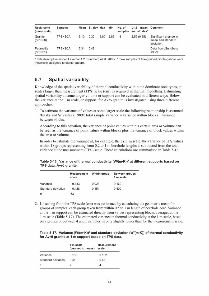
5.7 SpatialvariabilityKnowledge of the spatial variability of thermal conductivity within the dominant rock types, at scales larger than measurement (TPS) scale (cm), is required in thermal modelling. Estimating spatial variability at some larger volume or support can be evaluated in different ways. Below, the variance at the 1 m scale, or support, for Ävrö granite is investigated using three different approaches.
1. To estimate the variance of values at some larger scale the following relationship is assumed /Isaaks and Srivastava 1989/: total sample variance = variance within blocks + variance between blocks.
According to this equation, the variance of point values within a certain area or volume can be seen as the variance of point values within blocks plus the variance of block values within the area or volume.
In order to estimate the variance at, for example, the ca. 1 m scale, the variance of TPS values within 18 groups representing from 0.2 to 1 m borehole lengths is subtracted from the total variance at the measurement (TPS) scale. These calculations are summarised in Table 5-16.
Table5‑16. Varianceofthermalconductivity(W/(m·K))²atdifferentsupportsbasedonTPSdata.Ävrögranite.
Measurementscale
Withingroup Betweengroups,1mscale
Variance 0.183 0.023 0.160Standard deviation 0.428 0.151 0.400
n 63
2. Upscaling from the TPS scale (cm) was performed by calculating the geometric mean for groups of samples, each group taken from within 0.5 to 1 m length of borehole core. Variance at the 1 m support can be estimated directly from values representing blocks averages at the 1 m scale (Table 5-17). The estimated variance in thermal conductivity at the 1 m scale, based on 7 groups of between 4 and 5 samples, is only slightly lower than for the measurement scale.
Table5‑17. Variance(W/(m·K))²andstandarddeviation(W/(m·K))ofthermalconductivityforÄvrögraniteat1msupportbasedonTPSdata.
1mscale(geometricmeans)
Measurementscale
Variance 0.166 0.182Standard deviation 0.41 0.43
n 7 34

42
Figure 5-19 illustrates the variability within groups comprising four or more samples from a length of borehole core less than 1 m. The red box in Figure 5-19 represents values at the 1 m scale, 7 values in total, which can be compared with the somewhat larger variability present at the sample scale, and represented by the green box and its whiskers.
�. Using the thermal conductivity data from density loggings, a variance vs. scale diagram can be constructed (Figure 5-20). From this diagram, the variance at the 1 m scale can be estimated to approximately 0.1�5 (W/(m·K))². Variances estimated using this regression model may be underestimated due to the restricted density interval used to calculate thermal conductivity.
Figure 5‑19. Upscaling of TPS measurements from cm scale to 1 m scale for Ävrö granite. Seven groups of TPS measurements (grey boxes), each representing approximately 1 m, are used to estimate variability in thermal conductivity at the 1 m scale (red box). This can be compared with the total variability at the sample scale (green box). The middle line of a box represents the median, the upper and lower limits of a box the upper and lower quartiles respectively, and the whiskers correspond to the range of values.
Figure 5‑20. Variability of thermal conductivity within Ävrö granite based on calculated values determined from density loggings.
4�
The three different methods for estimating variance at the 1 m support yield rather similar results, between 0.1� and 0.17 (W/(m·K))². More important is that, independent of the method used, the variance at the 1 m scale is shown to comprise a large proportion of the total sample variance, which is about 0.18 (W/(m·K))². In other words, only a small part (10–20%) of the variability present at the cm scale is evened out at the 1 m scale.
5.8 HeatcapacityHeat capacity has been calculated from diffusivity and conductivity measurements using the TPS method. In Table 5-18 the heat capacity results from all samples are summarised /Adl-Zarrabi 2005abc, Dinges 2005, Sundberg et al. 2006/. The data includes 56 new samples from the Laxemar subarea, 20 for Ävrö granite, 24 for rock type 5010�6, 9 for diorite-gabbro, and � for granite (501058). Usually, measurement of diffusivity and conductivity is done at 20°C, but for samples of quartz monzodiorite taken at the surface, the measurements were carried out at 2�°C. Some of the samples were sampled in groups of 2–5 samples from short sections of core, 0.2–1 m. The summary statistics may therefore be somewhat biased.
The newly obtained data for two rock types (501044 and 5010�6) has little effect on the means and standard deviations presented previously in model version 1.2 /Sundberg et al. 2006/. Data for diorite-gabbro indicate that this rock type has a higher heat capacity than other important rock types. The heat capacity data are normally distributed for Ävrö granite and fine-grained dioritoid, whereas for quartz monzodiorite and diorite-gabbro slightly better fits are given by lognormal distributions (Appendix A).
A tendency for heat capacity to increase slightly with increasing density was noted by /Sundberg 200�b/ for granitic and dioritic rocks at Äspö HRL. Since a clear relationship between thermal conductivity and density has also been established for Ävrö granite from both Äspö and Laxemar, it was considered prudent to investigate the possibility of a relationship between heat capacity and thermal conductivity. Unequivocal relationships cannot be demonstrated for any of the rock types, although weak positive correlations are noted for diorite-gabbro and fine-grained dioritoid. Data for Ävrö granite is plotted in Figure 5-21.
Table5‑18. Heatcapacity(MJ/(m3·K))ofdifferentrocktypes,calculatedfromtheTPSmethod.SamplesarefromboreholesKSH01A,KSH02,KAV01andKAV04A(Simpevarpsubarea),KLX02,KLX03,KLX04,KLX05andKLX06(Laxemarsubarea),KA2599G01(ÄspöHRL),bore‑holesfromtheprototyperepositorytunnel(ÄSPÖHRL)togetherwith10surfacesamples.
Rockcode
Rockname Samplelocation Arithmeticmean
St.dev. Max Min Numberofsamples
CommentL2.1
501030 Fine-grained dioritoid
Bore holes KSH01A, KSH02
2.23 0.10 2.40 2.03 26 No new samples
501033 Diorite/gabbro1
Boreholes KLX05, KLX06
2.46 0.11 2.65 2.32 9 All new samples
501036 Quartz monzodiorite
Boreholes KAV04A, KSH01A, KLX03, KLX05 and surface
2.27 0.12 2.60 2.00 39 24 new samples
501044 Ävrö granite Boreholes KAV01, KAV04A, KLX02, KLX03, KLX04, KLX05, KLX06, KA2599G01 and Äspö HRL prototype tunnel
2.24 0.14 2.52 1.81 88 20 new samples
501058 Granite Borehole KLX05 2.17 0.24 2.33 1.89 3 All new samples
1 Two samples of fine-grained diorite-gabbro (505102) were incorrectly assigned to rock type diorite-gabbro (501033).
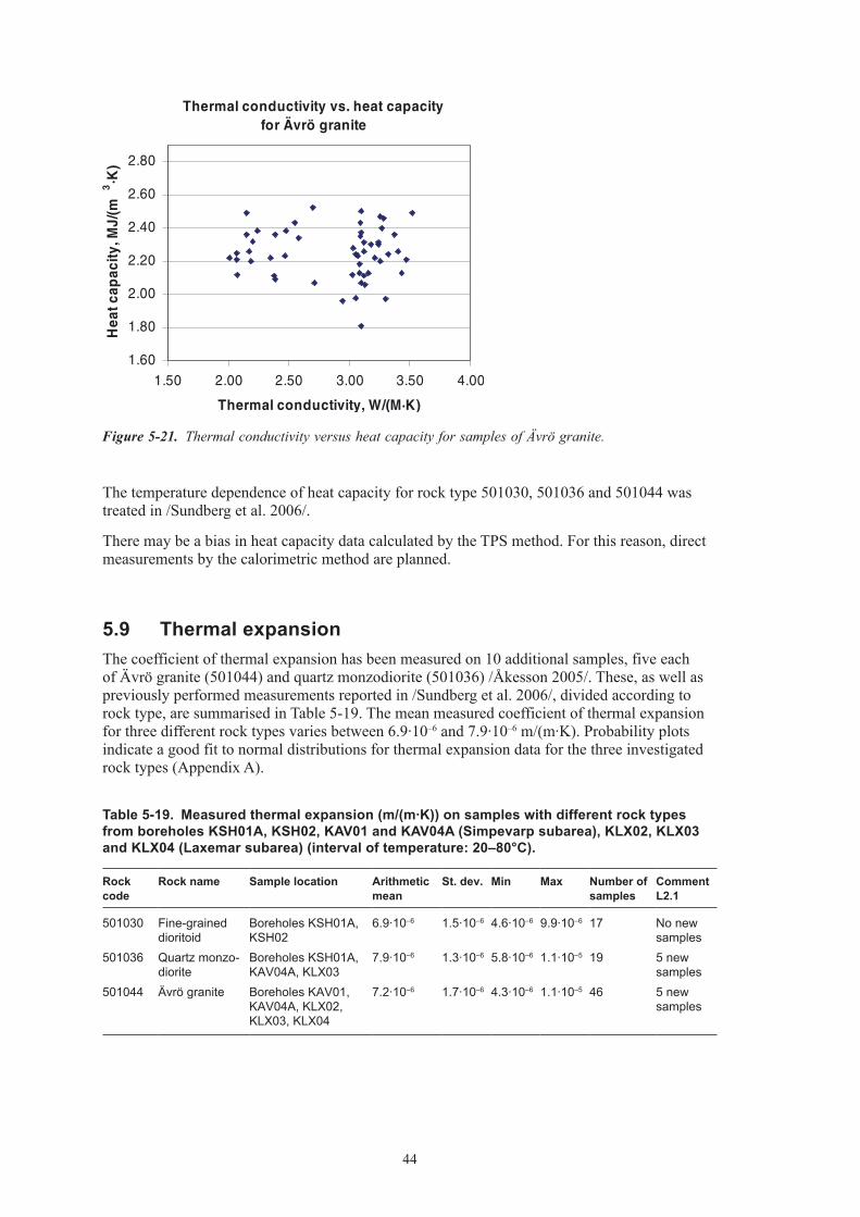
44
The temperature dependence of heat capacity for rock type 5010�0, 5010�6 and 501044 was treated in /Sundberg et al. 2006/.
There may be a bias in heat capacity data calculated by the TPS method. For this reason, direct measurements by the calorimetric method are planned.
5.9 ThermalexpansionThe coefficient of thermal expansion has been measured on 10 additional samples, five each of Ävrö granite (501044) and quartz monzodiorite (5010�6) /Åkesson 2005/. These, as well as previously performed measurements reported in /Sundberg et al. 2006/, divided according to rock type, are summarised in Table 5-19. The mean measured coefficient of thermal expansion for three different rock types varies between 6.9·10–6 and 7.9·10–6 m/(m·K). Probability plots indicate a good fit to normal distributions for thermal expansion data for the three investigated rock types (Appendix A).
Table5‑19. Measuredthermalexpansion(m/(m·K))onsampleswithdifferentrocktypesfromboreholesKSH01A,KSH02,KAV01andKAV04A(Simpevarpsubarea),KLX02,KLX03andKLX04(Laxemarsubarea)(intervaloftemperature:20–80°C).
Rockcode
Rockname Samplelocation Arithmeticmean
St.dev. Min Max Numberofsamples
CommentL2.1
501030 Fine-grained dioritoid
Boreholes KSH01A, KSH02
6.9·10–6 1.5·10–6 4.6·10–6 9.9·10–6 17 No new samples
501036 Quartz monzo-diorite
Boreholes KSH01A, KAV04A, KLX03
7.9·10–6 1.3·10–6 5.8·10–6 1.1·10–5 19 5 new samples
501044 Ävrö granite Boreholes KAV01, KAV04A, KLX02, KLX03, KLX04
7.2·10–6 1.7·10–6 4.3·10–6 1.1·10–5 46 5 new samples
Figure 5‑21. Thermal conductivity versus heat capacity for samples of Ävrö granite.

45
A relationship between density and thermal conductivity for Ävrö granite is well established. In addition, recent investigations have indicated correlations between density and certain rock mechanic properties for the same rock type. However, plots of thermal expansion against density for three rock types, Ävrö granite included, reveal no clear evidence for any correlation between these two parameters (Figure 5-22).
5.10 Insitutemperature5.10.1 MethodandassessmentofreliabilityThe temperature profiles have been investigated for boreholes KLX05 and KLX06. Corresponding investigations for boreholes KLX01 to KLX04 were presented in /Sundberg et al. 2006/. Temperature was measured by fluid temperature loggings. The measured data has been filtered. The filtering method used and the method of calculation of the temperature gradients for 9 m sections are described in /Mattson and Keisu 2005b/ and /Mattsson 2005/.
Large differences in logged temperature for the same depth in different boreholes has been previously noted /Sundberg et al. 2006/. Uncertainties associated with the data were judged to be high. For this reason, the temperature loggings from KLX01 to KLX06 have been evaluated with regard to their reliability, see Table 5-20. Parameters considered were 1) errors associated with logging probe and 2) time between drilling and logging. For KLX02, temperature loggings were performed on three occasions, 199�, 2002 and 200�. Data from the most recent logging, in 200�, is judged to be the most comparable to the loggings of the other boreholes (see /Sundberg et al. 2006/ for discussion), and is the one considered here.
Two different probes have been used for temperature logging, Century 8044 and Century 9042. According to Ramböll errors associated with Century 8044 are particularly large, ± 2°C (due to a design fault which affected the accuracy of calibration). Therefore, temperature loggings from KLX0�, 04 and 06, all logged using probe 8044, cannot be considered to be reliable. The same applies to KAV04A and KSH0�A reported in previous model versions. KAV04A was logged using a Century 9044 probe which had the same design problems as 8044 (Stenberg 2006). Century 9042 is considerably more accurate, less than ± 0.25°C (Stenberg 2006). Information regarding the quality of temperature logging in KLX01, which was logged in 1988 using a different type of probe, has not been obtained.
Figure 5‑22. Thermal expansion versus density for three rock types. Density data for these samples have not been reported to SICADA but are published in /Åkesson 2004abcdef, 2005/.

46
The period between the end of drilling activity and temperature logging must be sufficiently long in order to allow disturbances of the fluid temperature caused by drilling to stabilise. A rough rule of thumb is that logging should preferably not be carried out within 2 months after the end of drilling, and definitely not within the first �–4 weeks after drilling. Times for core drillings and fluid temperature loggings for the boreholes are given in Table 5-20. Based on this approximation it can be deduced that logging data from KLX01, KLX0� and KLX06 may have been collected before the temperature of the water in the boreholes had stabilised.
It is concluded that temperature loggings from KLX02 and KLX05 are the most reliable since both were logged using probe 9042 more than 2 months after the cessation of drilling. These are considered in more detail below and are used to draw conclusions regarding the temperature distribution in the rock mass. Data from the other boreholes are therefore excluded from subsequent evaluation.
5.10.2 ResultsTemperature is plotted against depth for KLX05 in Figure 5-2�. The y-axis in the figures illustrates depth below sea level (not the borehole length). The elevation (metres above sea level) at ground level for the starting point for the borehole is 17.6 m.
In Table 5-21 the temperatures at different depths are presented for the investigated boreholes in the Laxemar subarea. The mean temperature at different depths is calculated using data for KLX02 (200�) and KLX05 only. The results differ significantly from those reported in model version 1.2 /Sundberg et al. 2006/. It is apparent that the temperatures given by the approved loggings differ significantly to those of the rejected loggings. It is also interesting to note that for a given depth, KLX02 and KLX05 show almost identical temperatures.
Table5‑20. Evaluationoffluidtemperatureloggings.
Bore‑hole
Probe Riskforerrorsduetodesign/calibrationfault
Coredrilling:start‑stop
Fluidtem‑peraturelogging
Periodbetweendrillingandlogging
PFLlogging(withoutpumping)
Periodbetweendrillingandlogging
Judgementofqualityoffluidtemp.logging
KLX01 WellMac No info. available
19 Dec 1987 – 5 Feb 1988
10 Feb, 1988
5 days No data Poor quality
KLX02 (2003)
Century 9042
Low 1993 or earlier
30 June, 2003
Greater than 10 years
Test data only
Good quality.
KLX03 Century 8044
High 28 May – 7 Sept, 2004
30 Sept, 2004
3 weeks 6 Nov, 2004
2 months Poor quality. Verification provided by deviation from PFL data.
KLX04 Century 8044
High 13 Mar – 28 June, 2004
20 Oct, 2004
3–4 months No data Poor quality.
KLX05 Century 9042
Low 1 Oct 2004–22 Jan, 2005
6 April, 2005
2.5 months 14 April, 2005
2.5 months Good quality. Verification provided by similarity to PFL data.
KLX06 Century 8044
Yes 25 Aug–25 Nov, 2004
4 Jan, 2005
6 weeks 16 Feb, 2005
2.5 months Poor quality
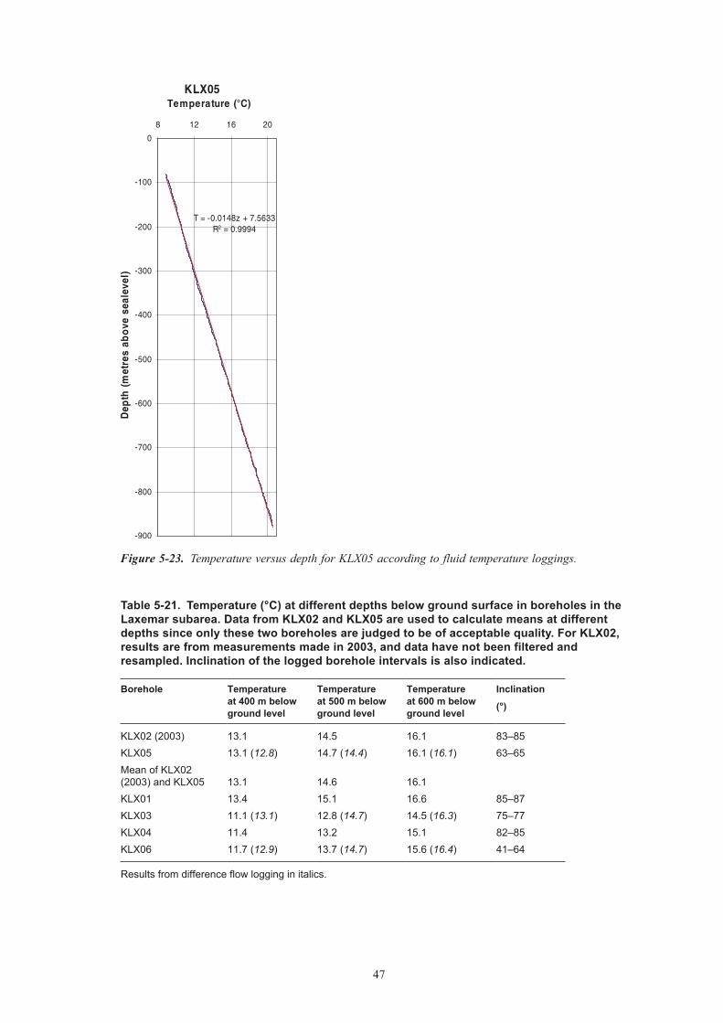
47
Table5‑21. Temperature(°C)atdifferentdepthsbelowgroundsurfaceinboreholesintheLaxemarsubarea.DatafromKLX02andKLX05areusedtocalculatemeansatdifferentdepthssinceonlythesetwoboreholesarejudgedtobeofacceptablequality.ForKLX02,resultsarefrommeasurementsmadein2003,anddatahavenotbeenfilteredandresampled.Inclinationoftheloggedboreholeintervalsisalsoindicated.
Borehole Temperatureat400mbelowgroundlevel
Temperatureat500mbelowgroundlevel
Temperatureat600mbelowgroundlevel
Inclination
(°)
KLX02 (2003) 13.1 14.5 16.1 83–85KLX05 13.1 (12.8) 14.7 (14.4) 16.1 (16.1) 63–65Mean of KLX02 (2003) and KLX05
13.1
14.6
16.1
KLX01 13.4 15.1 16.6 85–87KLX03 11.1 (13.1) 12.8 (14.7) 14.5 (16.3) 75–77KLX04 11.4 13.2 15.1 82–85KLX06 11.7 (12.9) 13.7 (14.7) 15.6 (16.4) 41–64
Results from difference flow logging in italics.
Figure 5‑23. Temperature versus depth for KLX05 according to fluid temperature loggings.

48
For boreholes KLX0�, KLX05 and KLX06, temperature data is available from difference flow loggings, or Posiva flow log (PFL) /Rouhiainen et al. 2005, Sokolnicki and Rouhiainen 2005ab/. Difference flow logging data (downwards, without pumping) for borehole KLX05 (Figure 5-24 and Table 5-21) indicate a reasonably good correspondence with fluid temperature data. In comparison, PFL data for KLX0� and KLX06 display large discrepancies with the fluid temperature data (Table 5-21). The PFL data thus provides support for the judgements made above regarding the reliability of temperature data from fluid temperature loggings.
Vertical temperature gradient data is being recalculated due to an error in the formula used previously. Data was unavailable from SICADA at the time of writing. It is recommended here that only gradient data from KLX02 and KLX05 are evaluated because of the errors associated with the other boreholes.
Figure 5‑24. Temperature versus depth for KLX05. Temperature has been measured by fluid tempera-ture and resistivity loggings, and by PFL measurement.

49
6 Thermalmodellingoflithologicaldomains
6.1 Modellingassumptionsandinputfromotherdisciplines6.1.1 GeologicalmodelThe rock domain model from the Laxemar site descriptive model version 1.2 forms the geo-metrical base for the thermal model and is described briefly in Chapter 4, and in greater detail in /SKB 2006/. The Laxemar subarea west of the plastic deformation zones (domains RSMP01 and RSMP02) is characterised by five lithological domains as described in Table 6-1 and illustrated in Figure 4-2. Three domains dominate the rock volume, namely RSMA, RSMD and RSMM.
In total, six boreholes were used for purposes of thermal modelling of domains. Compared with model version Laxemar 1.2, two additional boreholes, KLX05 and KLX06, were available for thermal modelling. The geological boremap log of the boreholes, showing the distribution of dominant and subordinate rock types, together with a lithological domain classification of borehole intervals (Table 6-2) has, after modification, been used as input to the thermal modelling. The available data is considered to be representative of the domains, allowing the numerical subscript in domain names to be omitted.
In thermal model version 1.2, the characterisation of rock domains by borehole intervals was modified so as to better represent the variability in thermal properties present within domains RSMA and RSMD (Table 6-�). Having only a minor component of rock type diorite/gabbro (5010��), the two RSMM domain intervals in KLX0� (100–800 m) were allocated to domain RSMA (dominated by Ävrö granite) and domain RSMD (dominated by quartz monzodiorite) respectively. For this reason modelling of domain RSMM has had to rely on estimates of typical rock type composition derived primarily from surface geological mapping /Wahlgren et al. 2005a/. For domain RSME borehole data is not available, so even in this case a rough estimate /Wahlgren et al. 2005a/ of rock type composition forms the basis for the thermal modelling. The same procedure is adopted for the current model version.
Table6‑1. Nomenclatureofrockdomainsreferredtointhisreport.
Domain Description
RSMA Dominated by Ävrö graniteRSMBA Mixture of Ävrö granite and fine-grained dioritoid
RSMD Dominated by quartz monzodioriteRSME Dominated by diorite/gabbroRSMM Mixed zone with large fraction of diorite/gabbro
Table6‑2. Boreholesclassifiedbydomain/SKB2006/.
Domain Borehole Comment
RSMA KLX01 0–1,078 m KLX02 200–540, 960–1,450 m KLX04 100–992 m KLX06 102–965 m
Based on subdomain RSMA01
RSMBA KLX02 540–960 m Based on subdomain RSMBA03
RSMD KLX02 1,450–1,700 m KLX03 800–1,000 m KLX05 473–1,000 m
Based on subdomain RSMD01
RSMM KLX03 100–620 m (A) KLX03 620–800 m (D) KLX05 100–473 m (A)
Based on subdomain RSMM01

50
Table6‑3. Datausedforcharacterisationofrockdomainsformodellingofthermalproperties.
Domain Sourceofdataformodelling
RSMA KLX01 0–701 m KLX02 200–540, 960–1,000 m KLX03 100–620 m KLX04 100–990 m KLX06 102–965 m
RSMBA KLX02 540–960 m
RSMD KLX03 620–1,000 m KLX05 473–1,000 m
RSMM Estimates of typical rock type compositions from geological mapping /Wahlgren et al. 2005a/.
RSME Estimates of typical rock type compositions from geological mapping /Wahlgren et al. 2005a/.
Rock type distributions of the five lithological rock domains are illustrated in Table 6-4 and Table 6-5 where the dominant rock types are marked in red. For rock type compositions of the borehole intervals constituting each lithological domain (also calculated in the thermal domain modelling), see Section 6.�.1.
Table6‑4. Rocktypepercentages(%)usedinthethermaldomainmodellingfordomainsRSMA,RSMBAandRSMD.Dominantrocktypesaremarkedinred.
Rockname DomainRSMA(Ävrögranite)
DomainRSMBA(MixtureofÄvrögraniteandFine‑graineddioritoid)
DomainRSMD(Quartzmonzodiorite)
Modelling Modelling Modelling
Ävrö granite 75.1 57.93 1.05Fine-grained dioritoid 0.92 32.17 0.57Quartz monzodiorite 3.23 81.7Pegmatite 0.41 0.12 3.03Diorite/gabbro 2.24Fine-grained diorite-gabbro 7.95 7.86 3.33Granite 6.02 0.28Fine-grained granite 4.17 1.93 10.0
Table6‑5. Rocktypepercentages(%)usedinthethermaldomainmodellingfordomainsRSMEandRSMM.Dominantrocktypesaremarkedinred.
Rockname DomainRSME(diorite/gabbro)
DomainRSMM(Mixedzonewithlargefractionofdiorite/gabbro)
Modelling² Modelling²
Ävrö granite 53Fine-grained dioritoid 2Quartz monzodiorite 27Pegmatite 0Diorite/gabbro 95 12Fine-grained diorite-gabbro 0Granite 5Fine-grained granite 5 1
² Based on rough estimates from surface geological mapping /Wahlgren et al. 2005a/.

51
6.1.2 BoreholedataIn boreholes where Ävrö granite is present, both accurate density loggings and a lithological classification of the borehole are required in order to model thermal conductivity. In boreholes without Ävrö granite, only a rock classification of the borehole is required. For more details regarding boreholes KLX01 to KLX04 see /Sundberg et al. 2006/. For KLX05 and KLX06, rock type classifications as well as calibrated and filtered density loggings are available.
6.2 ModellingapproachfordomainpropertiesOf importance at the domain level is the scale at which the thermal conductivity is relevant for the heat transfer from the canister. On the basis of present knowledge /Sundberg et al. 2005a/, variability below 1 m seems to have little or no relevance for the canister temperature. Therefore, so as not to underestimate the scale effect, results mainly from 0.8 m scale are used in the domain modelling to derive representative thermal conductivity values. This is in accordance with previous model versions.
The methodology for thermal conductivity domain modelling and the modelling of scale dependency were developed for the Prototype Repository at the Äspö HRL /Sundberg et al. 2005a/. The methodology involves a base approach (main approach in /Sundberg et al. 2005a/) by which the mean thermal conductivity, as well as some of the spatial variabilty, at domain level is modelled, and a number of complementary approaches which are applied in order to evaluate the total spatial variability at domain level. Only the results from the base approach are presented in this model version.
Modelling according to the base approach is performed as outlined in Figure 6-1. Thermal conductivity values, both measured and calculated from modal analysis, are used to produce PDFs (Probability Density Functions) for rock types present in a domain. These PDFs are referred to as rock type models. For rock types for which a relationship has been demonstrated to exist between thermal conductivity and density, density loggings are used to calculate thermal conductivity according to the model described in Section 5.4. This implies that spatial variability within the rock type is considered.
A domain is assumed to be characterised by the borehole sections assigned to that domain. Each borehole section is divided into 0.1 m long segments and each segment is assigned a thermal conductivity value according to the lithological classification of that section. The principle for assignment of thermal properties is illustrated in Figure 6-1.
The next step is upscaling for a range of scales, from 0.1 m to approximately 60 m, performed as follows. The boreholes representing the domain are divided into a number of sections with a length corresponding to the desired scale. Thermal conductivity is calculated for each section as the geometric mean of the values at the 0.1 m scale. This gives the effective thermal conductivity at the desired scale. The mean and the variance of all sections at the desired scale are calculated. For each scale, the calculations are repeated n times with different assignment of thermal conductivity values at the 0.1 m scale (stochastic simulation). This produces representa-tive values of the mean and the standard deviation for the desired scale.
The base approach differs slightly depending on whether borehole density loggings can be used (domains RSMA and RSMBA, both dominated by Ävrö granite) or cannot be used (domain RSMD). The reason is that density loggings of Ävrö granite can be used for domain RSMA and RSMBA to take into account spatial correlation within the dominant rock type. This is not possible for domain RSMD (quartz monzodiorite), which is dominated by other rock types for which no reliable “within rock type” relationship is presently available. Therefore, the variance for domain RSMD is underestimated in the base approach. Even for domains RSMA and
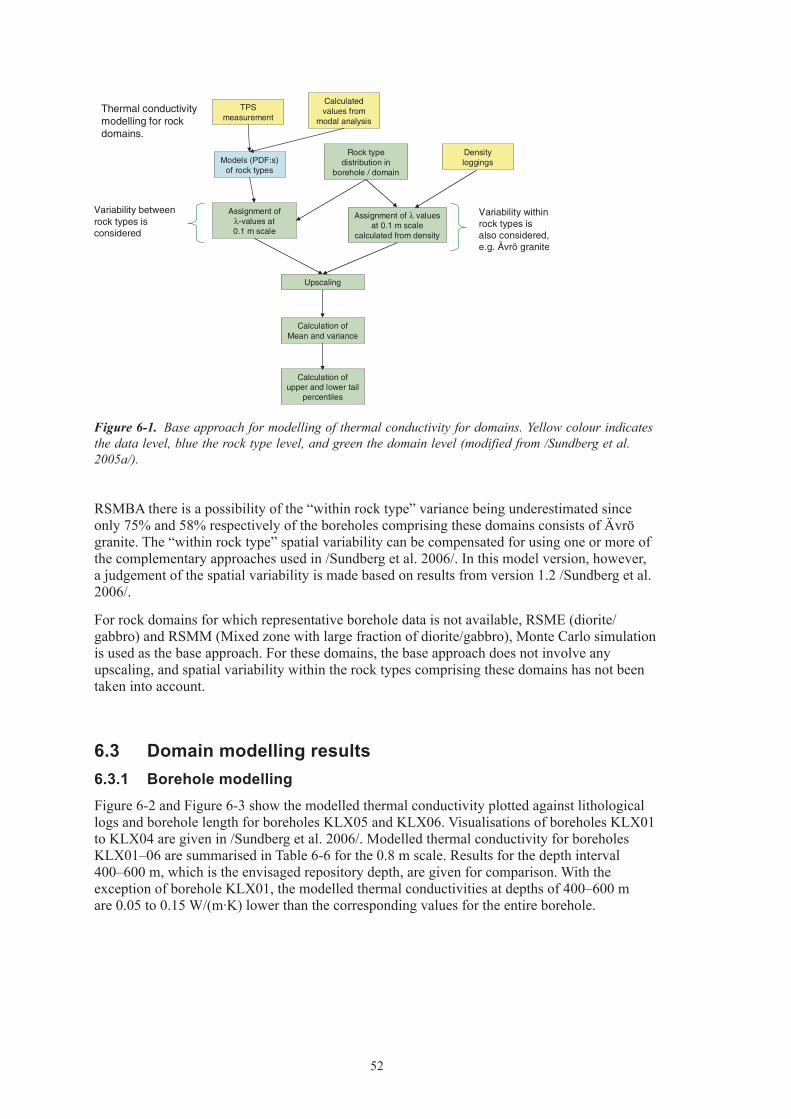
52
RSMBA there is a possibility of the “within rock type” variance being underestimated since only 75% and 58% respectively of the boreholes comprising these domains consists of Ävrö granite. The “within rock type” spatial variability can be compensated for using one or more of the complementary approaches used in /Sundberg et al. 2006/. In this model version, however, a judgement of the spatial variability is made based on results from version 1.2 /Sundberg et al. 2006/.
For rock domains for which representative borehole data is not available, RSME (diorite/gabbro) and RSMM (Mixed zone with large fraction of diorite/gabbro), Monte Carlo simulation is used as the base approach. For these domains, the base approach does not involve any upscaling, and spatial variability within the rock types comprising these domains has not been taken into account.
6.3 Domainmodellingresults6.3.1 BoreholemodellingFigure 6-2 and Figure 6-� show the modelled thermal conductivity plotted against lithological logs and borehole length for boreholes KLX05 and KLX06. Visualisations of boreholes KLX01 to KLX04 are given in /Sundberg et al. 2006/. Modelled thermal conductivity for boreholes KLX01–06 are summarised in Table 6-6 for the 0.8 m scale. Results for the depth interval 400–600 m, which is the envisaged repository depth, are given for comparison. With the exception of borehole KLX01, the modelled thermal conductivities at depths of 400–600 m are 0.05 to 0.15 W/(m·K) lower than the corresponding values for the entire borehole.
Figure 6‑1. Base approach for modelling of thermal conductivity for domains. Yellow colour indicates the data level, blue the rock type level, and green the domain level (modified from /Sundberg et al. 2005a/).

5�
Figure 6‑2. Exemplification of changes in thermal conductivity along borehole KLX05. Thermal conductivity is calculated as geometrical means over 2 metre long sections (moving average) from 0.1 m data. The results originate from one realisation only, and are based on both deterministic (for Ävrö granite) and stochastic (for other rock types) computations.

54
Figure 6‑3. Exemplification of changes in thermal conductivity along borehole KLX06. Thermal conductivity is calculated as geometrical means over 2 metre long sections (moving average) from 0.1 m data. The results originate from one realisation only, and are based on both deterministic (for Ävrö granite) and stochastic (for other rock types) computations.

55
Table6‑6. Summaryofthermalconductivity(W/(m·K))modellingresultsat0.8mscaleforboreholesKLX01,KLX02,KLX03,KLX04,KLX05andKLX06.
Borehole Scale,m Boreholelength Entireborehole Depthinterval400m–600mbelowsealevel
Mean Stdev Mean Stdev
KLX01 0.8 0–701 m 2.60 0.28 2.61 0.31KLX02 0.8 202–1,005 m 2.84 0.28 2.79 0.29KLX03 0.8 100–1,000 m 2.53 0.24 2.38 0.17KLX04 0.8 100–990 m 2.90 0.31 2.78 0.27KLX05 0.8 108–994 m 2.84 0.31 2.77 0.22KLX06 0.8 102–965 m 2.82 0.36 2.67 0.30
Figure 6-4 illustrates the modelled (according to the base approach) thermal conductivity plotted against elevation for the six Laxemar boreholes. The plotted thermal conductivity values are calculated as geometrical mean values for 50 metre long sections (moving average).
Figure 6‑4. Visualisation of large-scale changes in thermal conductivity with depth for six boreholes. Thermal conductivity is expressed as moving geometrical mean calculations over 50 meter long sections. For rock types other than Ävrö granite “within rock” spatial variability is not considered. Consequently the variability is underestimated for some borehole sections, e.g. lower parts of KLX03 and KLX05 dominated by quartz monzodiorite. The results are based on only one realisation.

56
In Figure 6-5, mean thermal conductivity for the six boreholes is plotted against depth. To take account of vertical depth for the different boreholes, thermal conductivity was calculated from 10 m vertical depth intervals before calculating means for all boreholes. The purpose of these plots is simply to describe large-scale trends in thermal conductivity. Spatial variability is considerably reduced because of the upscaling involved.
Taking all six boreholes into account there is a clear trend from 200 m to 500 m towards lower thermal conductivities. Lowest mean values (2.5 to 2.7 W/(m·K)) are found at depths of 450 m to 600 m. These generally lower values are apparent in most of the individual boreholes, with the exception of KLX05. The presence of lower conductivity varieties of Ävrö granite at these levels would largely explain this observation. Whether or not this is a feature of the entire rock volume within the Laxemar subarea is an issue that can only be resolved by additional boreholes.
6.3.2 Domainmodelling:baseapproachDomain RSMA, Ävrö granite
Domain RSMA is dominated by the rock type Ävrö granite (501044) which constitutes approximately 80% of the domain. The modelling of domain RSMA is based on data from five boreholes: KLX01, KLX02, KLX0�, KLX04 and KLX06. Approximately 97.5 % of the thermal conductivity values for Ävrö granite are computed from density loggings. For the rock type distribution of the domain and of the boreholes which constitute the domain, see Table 6-7.
Figure 6‑5. Visualisation of changes in mean thermal conductivity with vertical depth for six boreholes. Thermal conductivity values are expressed as the means of the same 10 m intervals (vertical depth) in six boreholes. The thermal conductivities for the 10 m intervals in each borehole are geometrical mean calculations over 10 meter long depth intervals. The results are based on only one realisation for each borehole.

57
Modelling results for domain A at the 0.8 m scale are presented in Table 6-7 and Figure 6-6. The lowest modelled thermal conductivity at this scale is 2.01 W/(m·K), which is the same as the lowest value measured in the laboratory for Ävrö granite. There is a large difference in thermal conductivity between boreholes making up domain RSMA. KLX01 and KLX0� have significantly lower mean thermal conductivity values than the other boreholes.
The bimodal distribution and large variance of thermal conductivity at domain level reflects the characteristic bimodal frequency distribution of the dominant rock type, i.e. Ävrö granite.
Table6‑7. ModellingresultsfordomainRSMA(Laxemarsubarea)anditscomprisingboreholesections:meanandstandarddeviationofthermalconductivity(W/(m·K))atdifferentscalesandrocktypedistributionsinpercent.
Rockname DomainRSMA KLX01 KLX02 KLX03 KLX04 KLX06Boreholeinterval1–701m 201.5–540m
960–1,000m100–620m 100–990m 102–965m
Percentagesofrocktypes
Ävrö granite (501044) 75.1 80.0 96.4 92.1 72.2 54.3Fine-grained dioritoid (501030) 0.9 0 0 0.4 3.1 0.1Quartz monzodiorite (501036) 3.2 0 0 0.5 11.9 0Pegmatite (501061) 0.4 0.4 0.2 0.1 0.3 0.9Diorite/gabbro (501033) 2.2 6.4 0 4.9 0.6 0Fine-grained diorite-gabbro (505102) 7.9 9.1 2.5 0.6 2.8 19.1Granite (501058) 6.0 0 0 0.1 4.0 19.2Fine-grained granite (511058) 4.2 4.1 1.0 1.3 5.0 6.4
ThermalconductivityMean(0.1mscale) 2.75St.dev 0.43Mean(0.8mscale) 2.75 2.60 2.89 2.40 2.90 2.82St.dev 0.35 0.28 0.30 0.20 0.22 0.36Mean(2mscale) 2.74St.dev 0.33
Figure 6‑6. Histogram of thermal conductivities for domain RSMA at the 0.8 m scale using the base approach.

58
The impact of scale on the means and standard deviations of thermal conductivity has been described previously /Sundberg et al. 2006/. In particular, the reduction in standard deviation that occurs as a result of upscaling is significant, the differences being greatest between 0.1 and 2 m, see Table 6-7.
A tendency towards lower thermal conductivities at depths of 450 m to 650 m is apparent in all boreholes making up domain A, see Figure 6-7. This tendency is even more apparent if the means for each vertical depth interval, using all boreholes sections making up the domain, are plotted against depth, see Figure 6-8. It should be noted that the above mentioned diagrams illustrate the large-scale trends in thermal conductivity only.
Domain RSMBA, Mixture of Ävrö granite and fine-grained dioritoid
Dominant rock types in domain RSMBA are Ävrö granite (501044) and fine-grained dioritoid (5010�0). Domain RSMBA is represented by borehole section 540–960 m in KLX02 (subdomain RSMBA0�), described in /Sundberg et al. 2006/. No additional data for this domain has been obtained. However, modelling has been repeated so as to incorporate both the revised rock type models and the new density relationship for Ävrö granite.
Modelling results for the domain at the 0.8 m scale is presented in Table 6-8 and Figure 6-9. Again there is the tendency towards bimodality in the distribution of modelled values.
Figure 6‑7. Visualisation of large-scale changes in thermal conductivity with depth for boreholes sec-tions belonging to domain A. Thermal conductivity is expressed as moving geometrical mean calcula-tions over 50 meter long borehole sections. The results are based on only one realisation. The diagram illustrates large-scale trends in thermal conductivity only. Spatial variability is considerably reduced.

59
Table6‑8. ModellingresultsfordomainRSMBAwithmeanandstandarddeviationofthermalconductivity(W/(m·K)).
DomainRSMBA(basedonboreholeinterval540–960minKLX02)Thermalconductivity,W/(m·K)0.1mscale 0.8mscale 2mscale
Mean 2.81 2.79 2.78St.dev 0.42 0.26 0.22
Figure 6‑8. Visualisation of changes in mean thermal conductivity with vertical depth for domain A based on five boreholes, KLX01, 02, 03, 04 and 06. Thermal conductivity values are expressed as the means of the same 10 m depth intervals (vertical depth). The thermal conductivities for the 10 m intervals in each borehole are geometrical mean calculations over 10 meter long depth intervals. The results are based on only one realisation.

60
Domain RSMD, Quartz monzodiorite
The dominant rock type in domain RSMD is quartz monzodiorite (5010�6). The domain is represented by a �80 m long borehole section (620–1,000 m) in KLX0�, and a 520 m long section in KLX05 of which quartz monzodiorite comprises ca 80%, see Table 6-9.
Modelling results for the domain at the 0.8 m scale are presented in Table 6-9 and Figure 6-10. The data distribution is characterised by a relatively low standard deviation and a long tail towards higher values. Except for Ävrö granite, spatial variability within the rock types comprising this domain has not been taken into account. The resulting variance includes variability due to rock type changes in the boreholes (“between rock type” variability) but the variability within each rock type is effectively and rapidly reduced when the scale is increased because of the random assignment of thermal conductivity values. Thus the modelling approach adopted for domain RSMD underestimates the variance at the 0.8 m scale.
Table6‑9. ModellingresultsforthedomainRSMDwithmeanandstandarddeviationofthethermalconductivity(W/(m·K))androcktypedistributionsinpercent.
Rockname DomainRSMD KLX03(620–1,000m)
KLX05(473–994m)
(Percentagesofrocktypes)
Ävrö granite (501044) 1.0 2.5 0Fine-grained dioritoid (501030) 0.6 0.7 0.5Quartz monzodiorite (501036) 81.7 84.4 79.8Pegmatite (501061) 3.0 1.1 4.4Diorite/gabbro (501033) 0 0 0Fine-grained diorite-gabbro (505102) 3.3 7.2 0.5Granite (501058) 0.3 0.6 0.1Fine-grained granite (511058) 10.0 3.6 14.7
Thermalconductivity,W/(m·K)0.1mscale 0.8mscale 2mscale
Mean 2.78 2.77 2.77St.dev 0.32 0.24 0.22
Figure 6‑9. Histogram of thermal conductivities for domain RSMBA at the 0.8 m scale using the base approach.

61
Domain RSME, Diorite/gabbro
Domain RSME is a small domain found in the north-eastern corner of the Laxemar subarea. The RSME domain is dominated by diorite/gabbro (5010��). There are no boreholes intercepting this domain so the rock type composition of 95% diorite/gabbro (5010��) and 5% fine-grained granite (511058) has been based on estimates from surface geological mapping /Wahlgren et al. 2005a/.
A rock type model of thermal conductivity for diorite-gabbro, used in the lithological domain modelling, has been constructed from a combination of both TPS measurements and SCA calculations. Using probability plots, the combined data has been shown not to correspond to a normal or lognormal distribution, see Figure 5-16 and Appendix A. For this reason, in modelling of domain E and M, both of which comprise a large fraction of diorite-gabbro, a custom distribution has been developed. The model is based on the values obtained from both TPS and SCA data, but also takes into consideration the proportion of different compositional varieties as indicated by the density loggings. The relatively few samples combined with the large spread in thermal conductivity values means that there are large uncertainties associated with the model.
Because of the lack of borehole data, the approach applied to the domains described above cannot be applied. Therefore, a simplified approach based on Monte Carlo simulation is used in modelling this domain. The results are presented in Table 6-10 and Figure 6-11.
Table6‑10. Thermalconductivity(W/(m·K))ofdomainRSME(diorite/gabbro).ModellingresultsfromMonteCarlosimulation.Notethatthescaleis<0.1m;noupscalingperformed.
Domain Mean St.dev
RSME 2.68 0.47
Figure 6‑10. Histogram of thermal conductivities for domain RSMD at the 0.8 m scale using the base approach.

62
The approach used for this domain does not take any account of variance reduction due to upscaling. Therefore, the quoted standard deviation most likely overestimates the dispersion at a larger scale for this domain since the data on which the rock model PDFs are based are for the TPS scale (dm scale). However, there are large uncertainties associated with both the estimated rock type composition of the domain and the rock type models.
Domain RSMM, Mixed zone with large fraction of diorite/gabbro
Borehole sections in both KLX0� (100–800 m) and KLX05 (100–47� m) have been assigned to domain RSMM but are considered not to be representative of the rock type composition for the domain as a whole. For this reason, the rock type abundances for domain RSMM are based on results from surface geological mapping /Wahlgren et al. 2005a/. The major rock types (see Table 6-5) are diorite/gabbro (12%), Ävrö granite (5�%) and quartz monzodiorite (27%) /Wahlgren et al. 2005a/. Because of the lack of borehole data a simplified approach based on Monte Carlo simulation is used in modelling this domain.
Since density loggings cannot be applied to Ävrö granite a probability density function (PDF) is used to model this rock type. Ävrö granite in the Laxemar subarea is characterised by a bimodal distribution, see Section 5.6.2. However, results from TPS measurements and density logging in boreholes KLX0� and KLX05, and from SCA calculations on surface samples of Ävrö granite in southern Laxemar /Sundberg et al. 2006/ indicate that the low thermal conductivity mode is dominant in the M domain. Therefore, a rock type model for Ävrö granite, based on data from density logging in KLX0� and KLX05 (Figure 5-14), has been specifically created for model-ling of domain M. A custom distribution has been used since none of the standard distributions described the data adequately.
The results of modelling are presented in Table 6-11 and Figure 6-12.
Table6‑11. Thermalconductivity(W/(m·K))ofdomainRSMM.ModellingresultsfromMonteCarlosimulation.Notethatthescaleis<0.1m;noupscalingperformed.
Domain Mean St.dev Comment
RSMM 2.56 0.33 Rock type model for Ävrö granite based on density loggings in KLX03 and KLX05
Figure 6‑11. Histogram of thermal conductivities for domain RSME from Monte Carlo simulation. (Scale < 0.1 m).
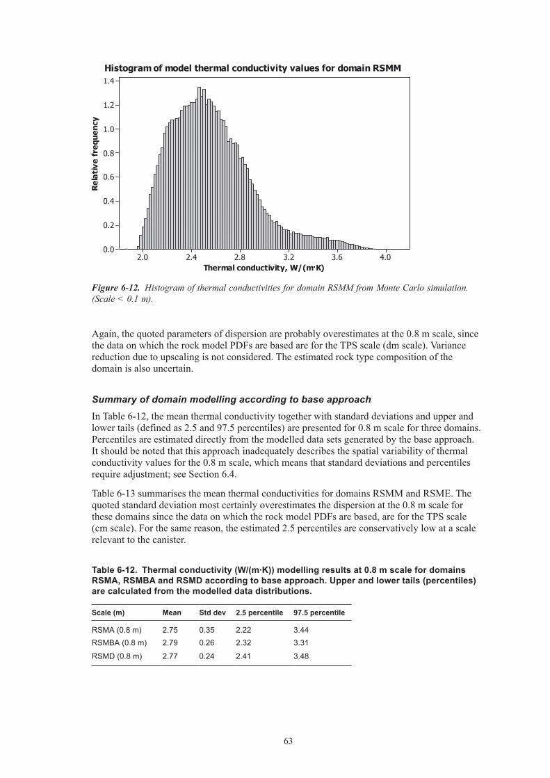
6�
Again, the quoted parameters of dispersion are probably overestimates at the 0.8 m scale, since the data on which the rock model PDFs are based are for the TPS scale (dm scale). Variance reduction due to upscaling is not considered. The estimated rock type composition of the domain is also uncertain.
Summary of domain modelling according to base approach
In Table 6-12, the mean thermal conductivity together with standard deviations and upper and lower tails (defined as 2.5 and 97.5 percentiles) are presented for 0.8 m scale for three domains. Percentiles are estimated directly from the modelled data sets generated by the base approach. It should be noted that this approach inadequately describes the spatial variability of thermal conductivity values for the 0.8 m scale, which means that standard deviations and percentiles require adjustment; see Section 6.4.
Table 6-1� summarises the mean thermal conductivities for domains RSMM and RSME. The quoted standard deviation most certainly overestimates the dispersion at the 0.8 m scale for these domains since the data on which the rock model PDFs are based, are for the TPS scale (cm scale). For the same reason, the estimated 2.5 percentiles are conservatively low at a scale relevant to the canister.
Table6‑12. Thermalconductivity(W/(m·K))modellingresultsat0.8mscalefordomainsRSMA,RSMBAandRSMDaccordingtobaseapproach.Upperandlowertails(percentiles)arecalculatedfromthemodelleddatadistributions.
Scale(m) Mean Stddev 2.5percentile 97.5percentile
RSMA (0.8 m) 2.75 0.35 2.22 3.44RSMBA (0.8 m) 2.79 0.26 2.32 3.31
RSMD (0.8 m) 2.77 0.24 2.41 3.48
Figure 6‑12. Histogram of thermal conductivities for domain RSMM from Monte Carlo simulation. (Scale < 0.1 m).
64
Table6‑13. Thermalconductivity(W/(m·K))modellingresultsfromMonteCarlosimulationfordomainsRSMEandRSMM.Thescaleis<0.1m.Noupscalinghasbeenimplemented,whichimpliesvariabilityoverestimatedforlargerscales.
Domain Mean St.dev 2.5percentile 97.5percentile
RSME 2.68 0.47 2.07 3.71
RSMM 2.56 0.3 2.06 3.41
6.4 Evaluationofdomainmodellingresults6.4.1 EstimationofmeanandstandarddeviationofthermalconductivityThe base approach is considered to produce reliable estimates of mean thermal conductivity for the five investigated domains. Variation in means as a function of scale is small. The base approach is believed to underestimate the standard deviation for domains RSMA and RSMBA, but particularly for RSMD, since the within rock variability is not fully accounted for. As regards domains RSME and RSMM, the base approach overestimates the variability, since no scaling up has been performed.
In the thermal modelling work in version Laxemar 1.2, four complementary approaches were used to evaluate the spatial variability at domain level /Sundberg et al. 2006/. This is particularly important for domains in which Ävrö granite is of minor importance. In this model version, however, no modelling has been done of the complementary approaches. Instead, a judgement of the spatial variability is made based on results from version 1.2 /Sundberg et al. 2006/. The same corrections applied to the standard deviations for each domain in model version 1.2 are used here to derive the revised standard deviations, (see Table 6-14).
Table 6-15 summarises the mean and revised standard deviation for each domain.
Table6‑14. Summaryofstandarddeviationsofthermalconductivity(W/(m·K))atdomainlevelbasedonmodellingresultsfromthebaseapproach,andcorrectedstandarddevia‑tionstotakeintoaccountspatialvariabilitywithinrocktypes.Thesecorrectionsaremadebasedonresultsfromthepreviousmodelversion(Laxemar1.2)sincenomodellingofcomplementaryapproacheshasbeenperformedinthecurrentmodelversion.
RSMA(Ävrögranite)
RSMBA(MixtureofÄvrögraniteandFine‑graineddioritoid)
RSMD(Quartzmonzodior‑ite)
RSME(Dioite/gabbro)
RSMM(mixdomain)
Comment
Base approach (scale: 0.8 m)
0.35 0.26 0.24 0.47
Monte Carlo sim.
0.33
Monte Carlo sim.
Underestimation for RSMA RSMBA and RSMD. Overestimation for RSME and RSMM.
Adjustements based on complementary approaches in model version 1.2.
0.01 0.04 0.04 n/a n/a No corrections made for domains RSME and RSMM
Corrected standard deviations
0.36 0.30 0.28 0.47 0.33

65
Table6‑15. Meanandrevisedstandarddeviationofthermalconductivity(W/(m·K))perdomain.FordomainsRSMA,RSMBAandRSMD,resultsapplytothe0.8mscaleandstandarddeviationsarerevisedonthebasisofresultsinmodelversion1.2/Sundbergetal.2006/.FordomainsRSME,RSMMresultsarebasedonascale<0.1m.
Domain Mean St.dev Comment
RSMA 2.75 0.36RSMBA 2.79 0.30
RSMD 2.77 0.28RSME 2.68 0.47 No changes in st. dev from MC simulationRSMM 2.56 0.33 No changes in st. dev from MC simulation
Observe that the above table is valid at 20°C. The thermal conductivity decreases slightly at higher temperatures, 1–5% per 100°C temperature increase.
6.4.2 EstimationoflowertailpercentilesofthermalconductivityIn model version 1.2, lower and upper tail percentiles for the revised standard deviations were estimated by applying corrections to the percentile values calculated from the modelled distribu-tions. The lower tail percentiles are of most interest as it is these that are critical for design purposes. This step is not repeated here, but it is worth mentioning that, in model version 1.2, for domains RSMA, RSMBA and RSMD, the revised 2.5 percentiles were between 0.0� and 0.11 W/(m·K) lower than those calculated from the modelled data distributions using the base approach, whereas for RSME and RSMM, the revised 2.5 percentiles were 0.2 W/(m·K) higher. Similar corrections could arguably be applied to the percentiles estimated from the base approach in this model version.
6.4.3 ComparisonwithpreviousmodelversionsA comparison of the thermal conductivity results for domain level presented in the site descrip-tive model Laxemar version 1.2 /SKB 2006/, and the current Laxemar 2.1 site descriptive model version is provided in Table 6-16. The differences in mean and standard deviation of thermal conductivity for domain RSMA between Laxemar 1.2 and Laxemar 2.1 are not insignificant. As regards the mean thermal conductivity, the amount by which this value has decreased in the current model version is similar to the magnitude of the bias suspected in model version 1.2 caused by a poorly constrained density – thermal conductivity relationship. Lower tail percentiles, calculated from modelled data distributions generated by the base approach, are also significantly lower. For example, the 2.5 percentile of 2.22 W/(m·K) presented here (Table 6-12) can be compared with the value of 2.�5 W/(m·K) given in model version 1.2 /Sundberg et al. 2006/.
For domain RSMD, both the mean and standard deviation are somewhat higher in Laxemar 2.1, an effect of the higher proportion of rock type fine-grained granite, which imparts a pronounced upper tail to the distribution, see Figure 6-10.
Although the mean thermal conductivity for domain RSMM shows little change from model version 1.2, variability, as expressed by standard deviation, is significantly higher. Uncertainty remains high for this domain due to the lack of representative borehole data and a poorly constrained statistical model for diorite-gabbro.
66
Table6‑16. Comparisonofmodellingresults(meanandstandarddeviation)forLaxemar1.2andLaxemar2.1sitedescriptivemodelversions.FordomainsRSMA,RSMBA,andRSMD,resultsapplytothe0.8mscale.FordomainsRSMEandRSMMresultsarebasedonMonteCarlosimulation,forwhichupscalingwasnotpossible.
Mean(W/(m·K)) St.dev(W/(m·K))Domain VersionL1.2 VersionL2.1 VersionL1.2 VersionL2.1
RSMA 2.82 2.75 0.29 0.36RSMBA 2.87 2.79 0.29 0.30RSMD 2.70 2.77 0.17 0.28RSME 2.45 2.68 0.29 0.47RSMM 2.58 2.56 0.22 0.33
Observe that the above table is valid at 20°C. The thermal conductivity decreases slightly at higher temperatures, 1–5% per 100°C temperature increase.
6.5 SummaryofdomainpropertiesThermal conductivityTable 6-15 summarises the recommended mean and standard deviation of thermal conductivity for each rock domain. Table 6-12 presents percentiles based on distributions from the base modelling approach. For a fuller discussion of these results, the reader is referred to the thermal modelling report for Laxemar version 1.2 /Sundberg et al. 2006/.
Heat capacity
Domain modelling of heat capacity has not been performed as part of this model version. Results presented in model version 1.2 /Sundberg et al. 2006/ for four domains, indicate a small range (2.2�–2.29 MJ/(m·K)) in mean heat capacity. New data indicates that diorite-gabbro (mean: 2.46 MJ/(m·K)) has a somewhat higher heat capacity than other major rock types; see Table 5-18. For domain M, which comprises a large proportion of diorite-gabbro, a slightly higher mean heat capacity value than that estimated in Laxemar 1.2 is expected. For other domains, the new data obtained is judged to have only a minor impact on the domain modelling results presented in model version 1.2.
Coefficient of thermal expansion
No domain modelling has been made. The mean measured coefficient of thermal expansion for three of the main different rock types varies between 6.9·10–6 and 7.9·10–6 m/(m·K) (Table 5-19), which is similar to results presented in version 1.2 /Sundberg et al. 2006/.
In situ temperatureDomain modelling has not been performed. The mean in situ temperatures at 400, 500 and 600 m depth below sea level are estimated at 1�.1, 14.6 and 16.1°C, respectively, which com-pares with 12.�, 1�.9 and 15.6°C, respectively, reported in version 1.2 /Sundberg et al. 2006/.
6.6 Discussion6.6.1 InterpretationofresultsFor a discussion of the uncertainties associated with thermal modelling in general, and model version Laxemar 1.2 in particular, the reader is referred to Chapter 6 in /Sundberg et al. 2006/. The current model version has produced some reductions in uncertainties. More specifically, the statistical relationship between density and thermal conductivity for Ävrö granite has been

67
improved, measurement data on rock types are considered to be more representative, statistical rock type models are in some cases more certain, and the rock volume is represented by more boreholes. In addition, errors associated with temperature logging have been defined, and poor quality logging data has been excluded from calculations of mean temperatures for various depths. A possible bias in heat capacity data has been recognised. Heat capacity is determined from thermal conductivity and diffusivity measurements, and not from direct measurement.
The revised model for the relationship between density and thermal conductivity for Ävrö granite, based on more plentiful data from the Laxemar subarea, better describes the rock volume in Laxemar, and has led to a reduction in bias associated with estimation of thermal conductivity from density logging. Comparison of measured values and modelled values show a better correspondence than in previous model versions /Sundberg et al. 2006/, especially for low thermal conductivity Ävrö granite. More measurements are planned with the purpose of both refining this relationship, particularly at the lower range of thermal conductivity, and of verifying the method.
The lowest measured thermal conductivity is 2.01 W/(m·K), for a sample of Ävrö granite from KLX0� in south Laxemar. This compares with the previous minimum of 2.16 W/(m·K) for a sample of Ävrö granite from Äspö. In the light of this new data, the lower 0.5 percentile value of ca 2.1 W/(m·K), derived by modelling of domain RSMA at scale 0.8 m, would appear reasonable.
The presence of considerable compositional variation within the Ävrö granite, from granite (sensu stricto) to quartz diorite, is well established /SKB 2006/. Not surprisingly, this is reflected in the wide spread of thermal conductivity values (2.0 to �.8 W/(m·K)) for this rock type, both measured on core samples and modelled from modal analyses and density loggings. A clear relationship between igneous rock type, as defined by /Streckeisen 1976/, and thermal conductivity has been established. Granites and granodiorites generally have conductivities of 2.9 W/(m·K) or greater, whereas quartz monzodiorites and quartz diorites have conductivities of 2.7 W/(m·K) or less.
Variation in both mineralogy and thermal properties within Ävrö granite in a north to south direction have been noted previously /SKB 2005, 2006, Sundberg et al. 2006/. Ävrö granite in boreholes in south Laxemar, KLX0� and KLX05, display low thermal conductivities, as do surface samples from the same area. A similar pattern is obvious in the north-eastern part of the Laxemar subarea. Boreholes in the central part of the subarea (KLX02 and KLX04) show generally high thermal conductivities for Ävrö granite, although the situation is more complex at depths below ca 500 m, where thermal conductivities tend to be lower and more variable.
Interpretation of plots of thermal conductivity versus depth for borehole intervals within domain RSMA indicates that thermal conductivity may be significantly lower at depths of 450 m to 600 m (Figure 6-8). However, analysis of additional boreholes is required to test whether this trend is a random effect of the positions of the available boreholes. Data from both recently drilled and planned boreholes should resolve this issue. The observed large-scale variations in thermal properties of Ävrö granite may have implications for the geological modelling of this rock type.
Uncertainties associated with the thermal modelling results of domain RSMM continue to be particularly large. Firstly, there is an incomplete understanding of the proportions of different rock types that comprise this domain. Secondly, the large variation in thermal conductivity measurements (TPS) for diorite-gabbro (2.25 to �.65 W/(m·K)) displayed by a relatively small number of samples means that statistical distribution models used for this rock in thermal modelling are still highly uncertain.
Diorite-gabbro is an important rock type from a thermal properties perspective since it occurs at repository depths in several boreholes. Density loggings indicate the possible existence of two or more distinct compositional types of diorite-gabbro, while an apparent correlation between density and thermal conductivity (Figure 5-9) opens the possibility of modelling spatial

68
variability in thermal conductivity with the aid of density loggings, in the same way as has been done for Ävrö granite /Sundberg et al. 2007/. Additional direct measurements (TPS) of diorite-gabbro to strengthen the new relationship between density and thermal conductivity are ongoing or planned. Modal analysis data for diorite-gabbro is also required so as to describe the relationship between mineralogy and thermal conductivity more precisely, especially for samples that have values that do not conform to the simple relationship of increasing thermal conductivity with increasing density.
The reason for bias in SCA results for several rock types remains to be resolved. An interesting feature revealed by recent data is that for Ävrö granite, bias is apparent in high conductivity samples but not in low conductivity samples. A plausible explanation for this is that the different compositional varieties contain plagioclase with somewhat different chemical compositions, and thus different thermal conductivities. This issue may be partly resolved by determining the anorthite content for a number of samples.
Evaluation of temperature loggings of the boreholes in Laxemar has shown deficiencies in the data for several of the boreholes. Data from KLX02 and KLX05 are considered to be the most reliable. Now that the technical problems which were causing the inaccurate data have been discovered and rectified, future data can be used to produce a more precise description of the in situ temperature distribution in the rock volume.
6.6.2 Remainingissuesanduncertainties–implicationsforfutureworkThe method used in this and earlier model versions /Sundberg et al. 2005b, 2006/ to evaluate and describe spatial variability of thermal properties at relevant scales is associated with uncertainties. More refined modelling strategies are required to describe the spatial variability at domain level more satisfactorily. An ongoing project (autumn 2006) dealing with modelling strategies aims to resolve these issues.
In modelling, upscaling of measurement scale (centimetre) data to metre scale involves uncertainties. This upscaling procedure leads to an over-reduction in spatial variability of thermal conductivity. Measurement of thermal conductivity at a scale more relevant for the dissipation of heat from the canister is of importance in order to minimise these uncertainties. For this reason, field measurements at larger scales are planned for autumn 2006. Investigations to evaluate the possible presence of anisotropy in thermal properties will be carried out at the same time. Because of the lack of strong fabrics, foliations or lineations, marked anisotropy is, however, not predicted.
Robust rock type models are highly dependent on representative data sets for each rock type. The representativity of data sets (both TPS and SCA) for some rock types has improved greatly compared to the previous model version, e.g. quartz monzodiorite, which has resulted in more certain models. Gaps remain, however. Laboratory measurements for some rock types, in particular for diorite-gabbro (see discussion above) and fine-grained diorite-gabbro, are required. It is also noted here that the error made in incorrectly assigning two samples (TPS measurements) of fine-grained diorite-gabbro (505102) from borehole KLX06 (Figure 5-1 and Section 5.2.2) to diorite-gabbro (5010��) is judged to have an insignificant impact on the thermal modelling results presented in this report. This error was discovered too late to allow revisions to be made to the modelling work, but instead will be corrected in the next model stage.
The high noise in the density logging data, on which modelling of spatial variability within Ävrö granite relies, is an important source of uncertainty. Improvements in this respect have been achieved with boreholes logged since July 2005 (KLX07 and subsequent boreholes), which will reduce uncertainty in future borehole modelling.
Alteration is present in all dominating rock types. According to Boremap mapping of available boreholes, a significant volume of rock (up to 25%) within the Laxemar subarea consists of weakly to strongly altered rocks. However, since alteration is generally associated with fracture
69
and deformation zones /SKB 2006/, and since the available boreholes may be over-representing the proportion of such zones, the importance of alteration may also be overestimated. Altered rocks are, on the other hand, extremely under-represented in the available thermal properties data, a factor which may significantly bias the results of the thermal modelling. Based on our understanding of the mineralogical changes associated with alteration, and the thermal conductivities of these alteration products, these altered rocks are expected to have higher thermal conductivity than unaltered equivalents. This has yet to be unambiguously demonstrated, however. Direct measurements (TPS) of thermal conductivity on altered rock samples are required. To improve our understanding of how mineral composition influences thermal properties, modal analysis should be performed on a selection of samples for which laboratory measurements are available. The effect of alteration may also be evaluated directly from mineral composition, using the SCA method. Modal analyses of sample pairs (one altered, the other fresh) reported by /Drake and Tullborg 2006/ may be used for this purpose.
For dominant rock types, for which density loggings cannot be used to evaluate spatial variability, sampling at different distances is required to produce variograms of spatial variability. This applies primarily to quartz monzodiorite.
Stress dependence on thermal conductivity and thermal expansion has not been investigated, although it is thought to be small. Measurement in the laboratory should be performed for verification purposes.
There is a potential bias in heat capacity data determined indirectly through conductivity and diffusivity measurements (TPS method). For this reason, direct measurements by the calorimetric method have been initiated.

71
References
Adl-ZarrabiB,2005a.Drill hole KLX0�A. Thermal properties: heat conductivity and heat capacity determined using the TPS method. SKB P-05-9�, Svensk Kärnbränslehantering AB.
Adl-ZarrabiB,2005b.Drill hole KLX05A. Thermal properties: heat conductivity and heat capacity determined using the TPS method. SKB P-05-126, Svensk Kärnbränslehantering AB.
Adl-ZarrabiB,2005c.Drill hole KLX06A. Thermal properties: heat conductivity and heat capacity determined using the TPS method. SKB P-05-129, Svensk Kärnbränslehantering AB.
DingesC,2005.Laxemar, Surface samples: Thermal properties: heat conductivity and heat capacity of surface samples determined using the TPS method. SKB P-05-169, Svensk Kärnbränslehantering AB.
DrakeD,TullborgE-L2005.Fracture mineralogy and wall rock alteration. Results from drill cores KAS04, KA1755A and KLX02. SKB P-05-174, Svensk Kärnbränslehantering AB.
DrakeD,TullborgE-L2006.Mineralogical, chemical and redox features of red-staining adjacent to fractures – Results from drill core KLX04. SKB P-06-02, Svensk Kärnbränslehantering AB.
EliassonT,1993.Mineralogy, geochemistry and petrophysics of red-coloured granite adjacent to fractures. SKB TR-9�-06, Svensk Kärnbränslehantering AB.
GustafssonS,1991.Transient plane source techniques for thermal conductivity and thermal diffusivity measurements of solid materials. Rev. Sci. Instrum. 62, p 797–804. American Institute of Physics, USA.
HoraiK,1971.Thermal conductivity of rock-forming minerals. J. Geophys. Res. 76, p 1278–1�08.
HoraiK,BaldridgeS,1972.Thermal conductivity of nineteen igneous rocks, Application of the needle probe method to the measurement of the thermal conductivity of rock. Estimation of the thermal conductivity of rock from the mineral and chemical compositions. Phys. Earth Planet. Interiors 5, p 151.
IsaaksEH,SrivastavaRM,1989.An introduction to applied geostatistics. Oxford University Press, New York.
MattssonH,2004.Interpretation of geophysical borehole data and compilation of petrophysical data from KSH0�A (100-1,000 m), KSH0�B, HAV09, HAV10 and KLX02 (200–1,000 m). Oskarshamn site investigation. SKB P-04-214, Svensk Kärnbränslehantering AB.
MattssonH,2005.Interpretation of geophysical borehole measurements from KLX06. Oskarshamn site investigation. SKB P-05-44, Svensk Kärnbränslehantering AB.
MattssonH,ThunehedH,Keisu,M,2005.Interpretation of geophysical borehole measure-ments and compilation of petrophysical data from KLX01, KLX0�, KLX04, HLX21, HLX22, HLX2�, HLX24, HLX25, HLX26, HLX27 and HLX28. Oskarshamn site investigation. SKB P-05-�4, Svensk Kärnbränslehantering AB.
MattssonH,Keisu,M,2005.Interpretation of geophysical borehole measurements from KLX05. Oskarshamn site investigation. SKB P-05-189, Svensk Kärnbränslehantering AB.
MunierR,StenbergL,StanforsR,MilnesAG,HermansonJ,TriumfC-A,2003.Geological site descriptive model. A strategy for the model development during site investigations. SKB R-0�-07, Svensk Kärnbränslehantering AB.
72
RouhiainenP,PöllänenJ,Sokolnicki,2005.Oskarshamn site investigation, Difference flow logging of borehole KLX0�, Subarea Laxemar. SKB P-05-67, Svensk Kärnbränslehantering AB.
SKB,2005.Program för fortsatta undersökningar av berggrund, mark, vatten och miljö inom delområde Laxemar. SKB R-05-�7, Svensk Kärnbränslehantering AB.
SKB,2006.Preliminary Site Description Laxemar subarea - version 1.2. SKB R-06-10, Svensk Kärnbränslehantering AB.
SokolnickiM,Rouhiainen,2005a. Difference flow logging in borehole KLX06 – subarea Laxemar. SKB R-05-74. Svensk Kärnbränslehantering AB.
SokolnickiM,RouhiainenP,2005b. Difference flow logging in borehole KLX05 – subarea Laxemar. SKB R-05-160. Svensk Kärnbränslehantering AB.
StreckeisenA,1976. To each plutonic rock its proper name. Earth Science Reviews 12, 1–��.
SundbergJ,1988.Thermal properties of soils and rocks, Publ. A 57 Dissertation. Department of Geology, Chalmers University of Technology and University of Göteborg, Sweden.
SundbergJ,2002.Determination of thermal properties at Äspö HRL. Comparison and evaluation of methods and methodologies for borehole KA 2599 G01. SKB R-02-27, Svensk Kärnbränslehantering AB.
SundbergJ,2003a.A strategy for the model development during site investigations version 1.0. SKB R-0�-10, Svensk Kärnbränslehantering AB.
SundbergJ,2003b.Thermal properties at Äspö HRL. Analysis of distribution and scale factors. SKB R-0�-17, Svensk Kärnbränslehantering AB.
SundbergJ,BackP-E,HellströmG,2005a.Scale Dependence and Estimation of Rock Thermal Conductivity. Analysis of Upscaling, Inverse Thermal Modelling and Value of Information with the Äspö HRL Prototype Repository as an Example. SKB R-05-82 Svensk Kärnbränslehantering AB.
SundbergJ,BackP-E,BengtssonA,Ländel,M,2005b. Oskarshamn site investigation. Thermal modelling of the Simpevarp Area – Supporting document for thermal model version 1.2. R-05-24, Geo Innova AB, Svensk Kärnbränslehantering AB, Stockholm.
SundbergJ,WrafterJ,BackP-E,LändellM,2006.Thermal modelling, Preliminary site description Laxemar subareas – version 1.2. R-06-1�, Svensk Kärnbränslehantering AB.
SundbergJ,EricssonLO,BackP-E,WrafterJ,2007.A method for estimation of thermal conductivity and its spatial variability in igneous rocks from in situ density logging. International Journal of Rock Mechanics and Mining Sciences (to be published).
WahlgrenC-H,HermansonJ,CurtisP,ForssbergO,TriumfC-A,TullborgE-L,DrakeH,2005a. Geological description of rock domains and deformation zones in the Simpevarp and Laxemar subareas. Preliminary site description, Laxemar subarea, version 1.2. SKB R-05-69, Svensk Kärnbränslehantering AB.
WahlgrenC-H,BergmanT,NilssonK,EliassonT,AhlM,EkströmM,2005b. Bedrock map of the Laxemar subarea and surroundings. SKB R-05-180, Svensk Kärnbränslehantering AB.
WahlgrenC-H,BergmanT,AhlM,2006.Modal and geochemical analyses of drill core samples 2005. Classification of rock types in KLX0�, KLX04, KLX06, KLX07A, KLX07B, KLX08 and KLX10. SKB R-06-07, Svensk Kärnbränslehantering AB.
ÅkessonU,2005.Drill hole KLX0�A Extensometer measurements of the coefficient of thermal expansion of rock. SKB P-05-95, Svensk Kärnbränslehantering AB.

7�
ÅkessonU,2004a.Drill hole KSH01A Extensometer measurements of the coefficient of thermal expansion of rock. SKB P-04-59, Svensk Kärnbränslehantering AB.
ÅkessonU,2004b.Drill hole KSH02 Extensometer measurements of the coefficient of thermal expansion of rock. SKB P-04-60, Svensk Kärnbränslehantering AB.
ÅkessonU,2004c.Drill hole KAV01 Extensometer measurements of the coefficient of thermal expansion of rock. SKB P-04-61, Svensk Kärnbränslehantering AB.
ÅkessonU,2004d.Drill hole KLX02 Extensometer measurements of the coefficient of thermal expansion of rock. SKB P-04-260, Svensk Kärnbränslehantering AB.
ÅkessonU,2004e.Drill hole KLX04 Extensometer measurements of the coefficient of thermal expansion of rock. SKB P-04-269, Svensk Kärnbränslehantering AB.
ÅkessonU,2004f.Drill hole KAV04 Extensometer measurements of the coefficient of thermal expansion of rock. SKB P-04-272, Svensk Kärnbränslehantering AB.
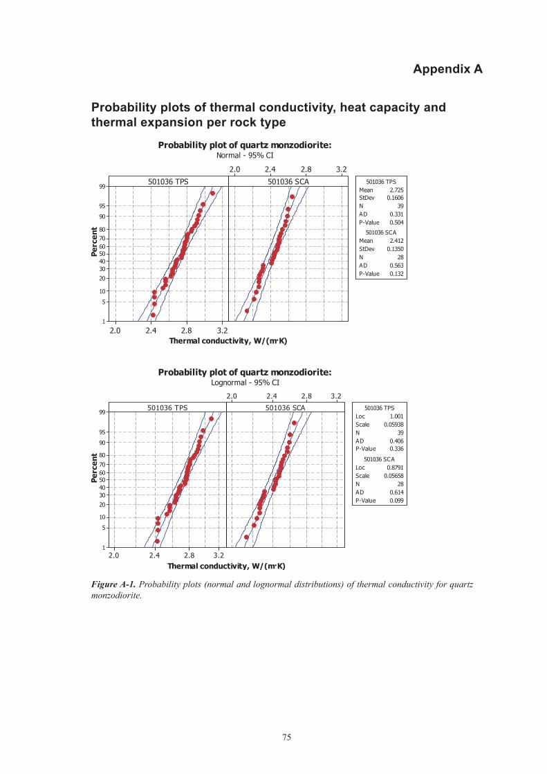
75
AppendixA
Probabilityplotsofthermalconductivity,heatcapacityandthermalexpansionperrocktype
Figure A‑1. Probability plots (normal and lognormal distributions) of thermal conductivity for quartz monzodiorite.

76
Figure A‑2. Probability plots (normal and lognormal distributions) of thermal conductivity for different rock types.

77
Figure A‑3. Probability plots (normal distributions) of heat capacity for different rock types.
Figure A‑4. Probability plots (lognormal distributions) of heat capacity for different rock types.
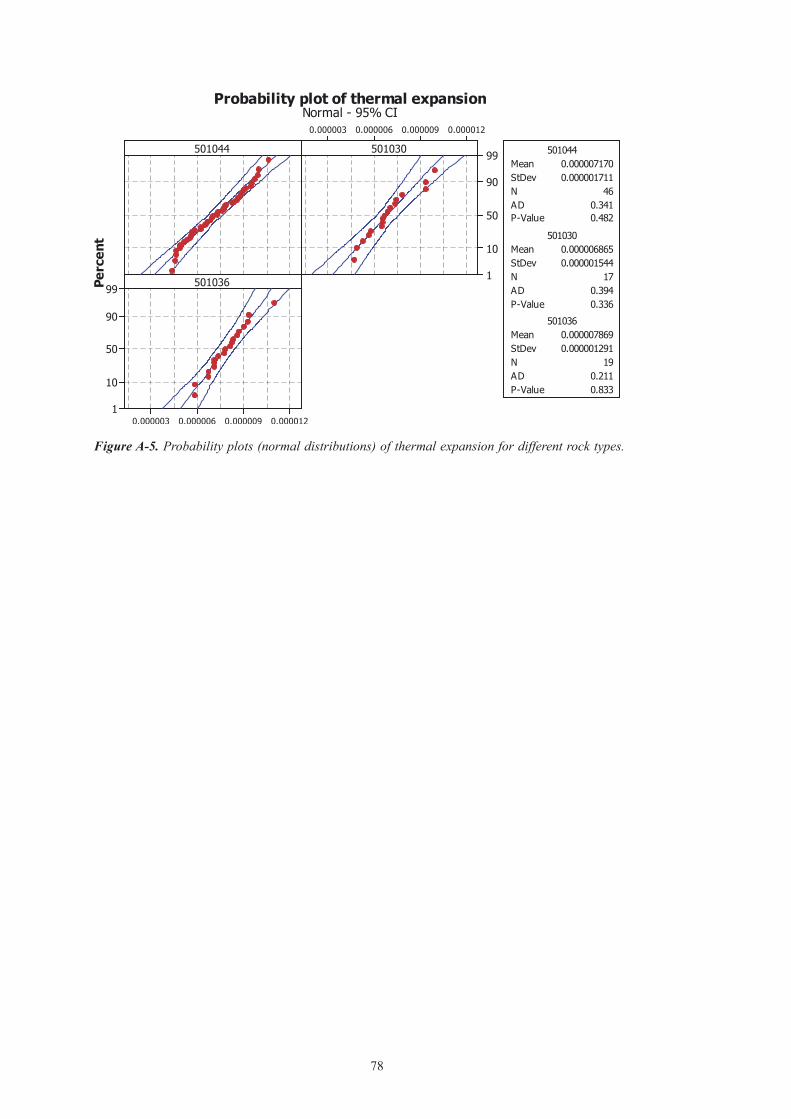
78
Figure A‑5. Probability plots (normal distributions) of thermal expansion for different rock types.